Astrophysics from Binary-Lens Microlensing

DISSERTATION

Presented in Partial Fulfillment of the Requirements for

the Degree Doctor of Philosophy in the Graduate

School of The Ohio State University

By

Jin Hyeok An, B.S.

*****

The Ohio State University

2002

Dissertation Committee: Approved by

Professor Andrew P. Gould, Adviser

Professor Darren L. DePoy Adviser

Professor Richard W. PoggeDepartment of Astronomy

ABSTRACT

Microlensing events, especially ones due to a lens composed of a binary

system can provide new channels to approach some of old questions in astronomy.

Here, by modeling lightcurves of three binary-lens microlensing events observed

by PLANET, I illustrate specific applications of binary-lens microlensing to real

astrophysical problems.

The lightcurve of a prototypical caustics-crossing binary-lens microlensing

event OGLE-1999-BUL-23, which has been especially densely covered by PLANET

during its second caustic crossing, enables me to measure the linear limb-darkening

coefficients of the source star in I and V bands. The results are more or less

consistent with theoretical predictions based on stellar atmosphere models,

although the nonlinearity of the actual stellar surface brightness profile may have

complicated the interpretation, especially for I band.

Next, I find that the model for the lightcurve of EROS BLG-2000-5, another

caustics-crossing binary-lens microlensing event, but exhibiting an unusually long

second caustic crossing as well as a very prominent third peak due to a close

ii

approach to a cusp, requires incorporation of the microlens parallax and the

binary orbital motion. Its projected Einstein radius is derived from the measured

microlens parallax, and its angular Einstein radius is inferred from the finite source

effect on the lightcurve, combined with an estimate of the source angular size given

by the source position on the color-magnitude diagram. The lens mass is found

by combining the above two quantities. This event marks the first case that the

parallax effects are detected for a caustic-crossing event and the first time that the

lens mass degeneracy has been broken.

The analysis of the lightcurve of MACHO 99-BLG-47, an almost normal

event with a well-covered short-duration anomaly near the peak, shows that it is

caused by an extreme-separation binary-lens. Although lightcurve anomalies that

are similar to what was observed for MACHO 99-BLG-47 may result from either

a planet around the lens or an extreme-separation binary, this result demonstrates

that the two classes of events can be distinguished in practice.

iii

Dedicated to everyone who reads this . . .

iv

ACKNOWLEDGMENTS

The author acknowledges that the completion of this work has been possible

thanks to contributions and advices made by numerous groups and individuals.

The author thanks all those individuals whose devotions and supports have been

invaluable to undertaking of this work.

The data upon which this work is based were largely obtained and

postprocessed through the collective efforts by the PLANET collaboration, which

also relies on the real-time event alerts issued by MACHO, OGLE, and EROS.

v

VITA

April 27, 1975 . . . . . . . . . . . . . . . . . . Born – Seoul, Republic of Korea

1997 . . . . . . . . . . . . . . . . . . . . . . . . . . . B.S. Astronomy, Seoul National University

1997 – 2001 . . . . . . . . . . . . . . . . . . . . Graduate Teaching and Research Associate,

The Ohio State University

2001 – present . . . . . . . . . . . . . . . . . Presidential Fellow, The Ohio State University

PUBLICATIONS

Research Publications

1. M. D. Albrow, J. An, J.-P. Beaulieu, et al., “PLANET observations of

microlensing event OGLE-1999-BUL-23: limb darkening measurement of the source

star.” the Astrophys. J., 549, 759, (2001).

2. M. Albrow, J. An, J.-P. Beaulieu, et al., “Hα equivalent width variation

across the face of a microlensed K giant in the Galactic Bulge.” the Astrophys. J.

Lett., 550, L173, (2001).

3. M. D. Albrow, J. An, J.-P. Beaulieu, et al., “Limits on the abundance

of Galactic planets from five years of PLANET observations.” the Astrophys. J.

Lett., 556, L113, (2001).

4. P. Martini, R. W. Pogge, S. Ravindranath, and J. H. An, “Hubble

Space Telescope observations of the CfA Seyferts 2s: near-infrared surface

photometry and nuclear bars.” the Astrophys. J., 562, 139, (2001).

vi

5. J. H. An, and A. Gould, “Microlens Mass Measurement using Triple-

Peak Events.” the Astrophys. J. Lett., 563, L111, (2001).

6. C. Han, H.-Y. Chang, J. H. An, and K. Chang, “Properties of mi-

crolensing light curve anomalies induced by multiple planets.” Mon. Not. of the R.

Astron. Soc., 328, 986, (2001).

7. A. Gould, and J. H. An, “Resolving microlens blends using image sub-

traction.” the Astrophys. J., 565, 1381, (2002).

8. B. S. Gaudi, M. D. Albrow, J. An, et al., “Microlensing constraints on

the frequency of Jupiter-mass companion: analysis of five years of PLANET

photometry.” the Astrophys. J., 566, 463, (2002).

9. J. H. An, M. D. Albrow, J.-P. Beaulieu, et al., “First microlens mass

measurement: PLANET photometry of EROS BLG-2000-5.” the Astrophys. J.,

572, 521, (2002).

10. M. D. Albrow, J. An, J.-P. Beaulieu, et al., “A short, non-planetary,

microlensing anomaly: observations and lightcurve analysis of MACHO 99-BLG-

47.” the Astrophys. J., 572, 1031, (2002).

11. J. H. An, and C. Han, “Effect of a wide binary companion on the as-

trometric behavior of gravitational microlensing events.” the Astrophys. J., 573,

351, (2002).

FIELDS OF STUDY

Major Field: Astronomy

vii

Table of Contents

Abstract . . . . . . . . . . . . . . . . . . . . . . . . . . . . . . . . . . . . . ii

Dedication . . . . . . . . . . . . . . . . . . . . . . . . . . . . . . . . . . . . iv

Acknowledgments . . . . . . . . . . . . . . . . . . . . . . . . . . . . . . . . v

Vita . . . . . . . . . . . . . . . . . . . . . . . . . . . . . . . . . . . . . . . vi

List of Tables . . . . . . . . . . . . . . . . . . . . . . . . . . . . . . . . . . xii

List of Figures . . . . . . . . . . . . . . . . . . . . . . . . . . . . . . . . . . xv

1 Introduction 1

2 Source Limb-Darkening Measurement: OGLE-1999-BUL-23 5

2.1 Introduction . . . . . . . . . . . . . . . . . . . . . . . . . . . . . . . . 5

2.2 Limb Darkening Measurement from Caustic-Crossing Microlensing . . 9

viii

2.3 OGLE-1999-BUL-23 . . . . . . . . . . . . . . . . . . . . . . . . . . . 12

2.3.1 Data . . . . . . . . . . . . . . . . . . . . . . . . . . . . . . . . 13

2.4 Lightcurve Analysis and Results . . . . . . . . . . . . . . . . . . . . . 16

2.4.1 Searching for χ2 Minima . . . . . . . . . . . . . . . . . . . . . 20

2.4.2 Solutions: χ2 Minimization . . . . . . . . . . . . . . . . . . . 21

2.5 Limb Darkening Coefficients Measurement . . . . . . . . . . . . . . . 32

2.6 Physical Properties of the Source Star . . . . . . . . . . . . . . . . . 39

2.7 Limb Darkening of the Source . . . . . . . . . . . . . . . . . . . . . . 43

3 Microlens Mass Measurement: EROS BLG-2000-5 49

3.1 Introduction . . . . . . . . . . . . . . . . . . . . . . . . . . . . . . . . 49

3.2 Overview . . . . . . . . . . . . . . . . . . . . . . . . . . . . . . . . . . 54

3.3 Measurement of Parallax from Triple-Peak Events . . . . . . . . . . . 56

3.4 Effect of Binary Orbital Motion . . . . . . . . . . . . . . . . . . . . . 62

3.5 EROS BLG-2000-5 . . . . . . . . . . . . . . . . . . . . . . . . . . . . 65

3.5.1 Data . . . . . . . . . . . . . . . . . . . . . . . . . . . . . . . 66

ix

3.6 Parameterization . . . . . . . . . . . . . . . . . . . . . . . . . . . . . 71

3.6.1 Description of Geometry . . . . . . . . . . . . . . . . . . . . . 72

3.6.2 The Choice of Fit Parameters . . . . . . . . . . . . . . . . . . 77

3.6.3 Terrestrial Baseline Parallax . . . . . . . . . . . . . . . . . . . 82

3.7 Measurement of the Projected Einstein Radius . . . . . . . . . . . . 87

3.8 Measurement of the Angular Einstein Radius . . . . . . . . . . . . . 92

3.9 The Lens Mass and the Lens-Source Relative Proper Motion . . . . . 99

3.10 The Kinematic Constraints on the Source Distance . . . . . . . . . . 101

3.11 Consistency between the Lens Mass and the Binary Orbital Motion . 106

3.12 Another Look at MACHO 97-BLG-41 . . . . . . . . . . . . . . . . . . 109

3.13 Summary . . . . . . . . . . . . . . . . . . . . . . . . . . . . . . . . . 112

4 Nonplanetary Microlensing Anomaly: MACHO 99-BLG-47 119

4.1 Introduction . . . . . . . . . . . . . . . . . . . . . . . . . . . . . . . . 119

4.2 MACHO 99-BLG-47 . . . . . . . . . . . . . . . . . . . . . . . . . . . 123

4.2.1 Observations and Data . . . . . . . . . . . . . . . . . . . . . 124

x

4.3 Analysis and Model . . . . . . . . . . . . . . . . . . . . . . . . . . . 128

4.4 Discussion . . . . . . . . . . . . . . . . . . . . . . . . . . . . . . . . . 136

4.5 Binary Lens vs. Binary Source . . . . . . . . . . . . . . . . . . . . . . 142

4.6 Close and Wide Binary Correspondence . . . . . . . . . . . . . . . . 143

4.7 Summary . . . . . . . . . . . . . . . . . . . . . . . . . . . . . . . . . 152

Bibliography 153

APPENDICES 158

A Fold-Caustic Magnification of Limb-Darkened Disk 158

B Determination of ς 161

C Microlens Diurnal Parallax 164

D Hybrid Statistical Errors 167

E Minimization with Constraints 170

xi

List of Tables

2.1 PLANET photometry of OGLE-1999-BUL-23. The predicted flux of

magnified source is F = FsA + Fb,0 + ηθs = Fs[A + bm + η(θs − θs,m)],

where A is magnification and θs is the FWHM of the seeing disk in

arcsec. The values of bm and η are evaluated for the best model (wide

w/LD), in Table 2.2. . . . . . . . . . . . . . . . . . . . . . . . . . . . 17

2.2 PLANET solutions for OGLE-1999-BUL-23 . . . . . . . . . . . . . . 25

2.3 Models in the neighborhood of the best-fit solution . . . . . . . . . . 26

3.1 PLANET I-band Photometry of EROS BLG-2000-5 . . . . . . . . . . 114

xii

3.2 Relations between Parameterizations. For simplicity, the reference

times, tc, for both systems are chosen to be the same: the time of

the closest approach to the cusp, i.e., (utc − ucusp) · utc = 0. The

additional transformation of the reference time requires the use of

equations (3.17) and (3.19). Figure 3.2 illustrates the geometry used

for the derivation of the transformation. The unit vector en points

toward the NEP while ew is perpendicular to it and points to the

west (the direction of decreasing ecliptic longitude). . . . . . . . . . . 115

3.3 PLANET Model Parameters for EROS BLG-2000-5 . . . . . . . . . . 116

3.4 Limb-Darkening Coefficients for EROS BLG-2000-5. The error bars

account only for the uncertainty in the photometric parameters

restricted to a fixed lens model, determined by the linear flux fit. . . . 117

3.5 Kinematic Characteristics of the Lens and the Source. The x-

direction is toward the Galactic center from the LSR, the y-direction

is the direction of the Galactic rotation, and the z-direction is toward

the north Galactic pole. The lens is assumed to be an M dwarf while

the source is a K3 giant. The quoted values for the disk components

are derived from Binney & Merrifield (1998). . . . . . . . . . . . . . . 118

4.1 Photometric data of MACHO 99-BLG-47. . . . . . . . . . . . . . . . 126

xiii

4.2 PLANET close-binary model of MACHO 99-BLG-47. We note that

the fact that χ2 ∼ dof results from our rescaling of the photometric

errorbars. However, we use the same scaling factor here and for

models described in Table 4.3 so the indistinguishableness between

two models is not affected by this rescaling. The uncertainties for

parameters are “1-σ error bars” determined by a quadratic fit of χ2

surface. . . . . . . . . . . . . . . . . . . . . . . . . . . . . . . . . . . 134

4.3 PLANET wide-binary model of MACHO 99-BLG-47. . . . . . . . . 135

xiv

List of Figures

2.1 Whole data set excluding later-time baseline points (2451338 <

HJD < 2451405), in I (top) and V (bottom) bands. Only the zero

points of the different instrumental magnitude systems have been

aligned using the result of the caustic crossing fit (§ 2.4.1); no attempt

has been made to account for either different amounts of blended light

or seeing corrections. . . . . . . . . . . . . . . . . . . . . . . . . . . 18

2.2 Fit of the caustic-crossing data to the six-parameter analytic curve

given by eq. (2.8). The time of second caustic crossing (tcc) and the

time scale of caustic crossing (∆t) are indicated by vertical lines. The

instrumental SAAO I-band flux, F18.4, is given in units of the zero

point I = 18.4. . . . . . . . . . . . . . . . . . . . . . . . . . . . . . . 22

xv

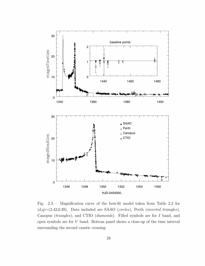
2.3 Magnification curve of the best-fit model taken from Table 2.2

for (d,q)=(2.42,0.39). Data included are SAAO (circles), Perth

(inverted triangles), Canopus (triangles), and CTIO (diamonds).

Filled symbols are for I band, and open symbols are for V band.

Bottom panel shows a close-up of the time interval surrounding the

second caustic crossing. . . . . . . . . . . . . . . . . . . . . . . . . . . 28

2.4 I-band lightcurves of the two “degenerate” models in SAAO

instrumental I magnitude. The solid line shows the best-fit model

of a wide binary lens, (d,q)=(2.42,0.39), and the dotted line shows

the close binary-lens model, (d,q)=(0.56,0.56). The filled circles show

SAAO data points. Both models are taken from Table 2.2 and use

the estimates of blending factors and baselines. The top panel is for

the whole lightcurve covered by the data, and the bottom panel is for

the caustic-crossing part only. . . . . . . . . . . . . . . . . . . . . . . 29

xvi

2.5 Lens geometries of the two “degenerate” models. The origin of the

coordinate system is the geometric center of the binary lens, and

the cross marks the center of the mass of the lens system. One

unit of length corresponds to θE. Closed curves are the caustics,

and the positions of the binary lens components are represented by

circles, with the filled circle being the more massive component. The

trajectory of the source relative to the lens system is shown by arrows,

the lengths of which are 2θE. . . . . . . . . . . . . . . . . . . . . . . . 30

2.6 Caustics of the two “degenerate” models with respect to the source

path shown as a horizontal line. The similarity of the lightcurves seen

in Fig. 2.4 is due to the similar morphology of the caustics shown here. 31

xvii

2.7 Solid line shows the lightcurve of the best-fit PLANET model (wide

w/LD), and the dotted line shows the PLANET close-binary model

(close w/LD). The models are determined by fitting PLANET data

only, but the agreement between the PLANET model (wide w/LD)

and OGLE data is quite good. On the other hand, OGLE data

discriminate between the two “degenerate” PLANET models so that

the wide-binary model is very much favored, in particular, by the

observations in (2451250 < HJD < 2451330). The baseline of the

PLANET model (wide w/LD) is, IOGLE = 17.852 ± 0.003, which is

consistent with the value reported by OGLE, IOGLE = 17.850 ± 0.024. 33

2.8 Residuals from PLANET models of OGLE-1999-BUL-23 around the

second caustic crossing. Top panel shows the residual for a model

incorporating linear limb darkening (wide w/LD) and lower panel

shows the same for a uniform disk model (wide no-LD). Both models

are taken from Table 2.2. Symbols are the same as in Fig. 2.3. The

residuals from the uniform disk are consistent with the prediction that

the source is limb-darkened while the remaining departures from the

limb-darkened model, which are marginally significant, may be due

to nonlinearity in the surface brightness profile of the source star. . . 36

xviii

2.9 Color-magnitude diagram (CMD) of the field centered on OGLE-

1999-BUL-23. Upper CMD is derived from 2′×2′ SAAO images,

and lower CMD is from 4′×4′ Canopus images. The positions of the

unlensed source (S), the baseline (B), blended light (BL) at median

seeing, and the center of red clump giants (RC), are also shown.

The extinction inferred from the (reddened) OGLE magnitude of the

source in the I band is, AI = 1.18, which implies E(V −I) = 0.792

assuming the extinction law AI = 1.49E(V −I). . . . . . . . . . . . . 41

xix

2.10 Comparison of linear limb-darkening coefficients. The measured value

from the best model is represented by a cross. One (solid line) and

two (dotted line) σ error ellipses are also shown. are displayed by

dashed lines (log g = 3.5). Model A is taken from Dıaz-Cordoves et

al. (1995) and Claret et al. (1995), B is from van Hamme (1993),

and C is from Claret (1998b). In particular, the predicted values in

the temperature range that is consistent with our color measurements

(Teff = 4820±110 K for log g = 3.0; Teff = 4830±100 K for log g = 3.5;

and Teff = 4850±100 K for log g = 4.0) are emphasized by thick solid

lines. Model C’ is by Claret (1998b) for stars of Teff = 4850 ± 100 K

for log g = 4.0. Although the measured value of the limb-darkening

coefficients alone favors this model, the model is inconsistent with our

estimation of the proper motion. . . . . . . . . . . . . . . . . . . . . . 44

xx

3.1 PLANET I-band lightcurve of EROS BLG-2000-5 (the 2000 season

only). Only the data points used for the analysis (“cleaned high-

quality” subset; see § 3.5.1) are plotted. Data shown are from SAAO

(circles), Canopus (triangles), YALO (squares), and Perth (inverted

triangles). All data points have been deblended using the fit result

– also accounting for the seeing correction – and transformed to the

standard I magnitude; I = Is−2.5 log[(F (t)−Fb)/Fs]. The calibrated

source magnitude (Is = 16.602) is shown as a dotted line. The three

bumps in the lightcurve and the corresponding positions relative to

the microlens geometry are also indicated. . . . . . . . . . . . . . . . 68

3.2 Geometry used for deriving the transformation shown in Table 3.2.

The direction of dtc is chosen to be the x-axis while πE lies parallel

to the direction of decreasing ecliptic longitude; ew. The reference

time, tc is the time of the closet approach to the cusp, ucusp. . . . . . 76

3.3 Prediction of deviations of lightcurves for SAAO and YALO from

the geocentric lightcurve for a chosen model. The solid curve is

the magnitude difference between the SAAO lightcurve and the

geocentric one, and the dotted curve is the same for YALO. Nominal

night portions (between 6 pm and 6 am local time) of the lightcurve

are highlighted by overlaid dots. . . . . . . . . . . . . . . . . . . . . . 85

xxi

3.4 Close-up of model lightcurves for the end of the second caustic

crossing. The solid curve is modeled for SAAO observations, the

dotted curve is for YALO, and the dashed curve is the geocentric

lightcurve. The timing of the end of the second crossing for SAAO is

earlier than for YALO by 11 minutes. For comparison purposes, all

the lightcurve are calculated assuming no blend. . . . . . . . . . . . . 86

3.5 Surface brightness profile of the source star. The thick solid curve

is the prediction indicated by the best fit model (see Table 3.4).

In addition, the variation of profiles with the parameters allowed

to deviate by 2-σ along the direction of the principal conjugate

is indicated by a shaded region. For comparison, also shown are

theoretical profiles taken from Claret (2000). The stellar atmospheric

model parameters for them are log g = 1.0, [Fe/H]= −0.3, and

Teff = 3500 K (dotted curve), 4000 K (short dashed curve), 4500 K

(long dashed curve). Note that the effective temperature of the source

is reported to be 4500 ± 250 K by Albrow et al. (2001b). . . . . . . . 89

xxii

3.6 “Magnitude” residuals from PLANET model of EROS BLG-2000-5.

Symbols are the same as in Fig. 3.1 The top panel shows the lightcurve

corresponding to the time of observations, the middle panel shows the

averaged residuals from 15-sequential observations, and the bottom

panel shows the scatters of individual residual points. . . . . . . . . . 90

3.7 Same as Fig. 3.6 but focuses mainly on the “anomalous” part of the

lightcurve. The middle panel now shows the daily averages of residuals. 91

xxiii

3.8 Geometry of the event projected on the sky. Left is Galactic east,

up is Galactic north. The origin is the center of mass of the binary

lens. The trajectory of the source relative to the lens is shown as

a thick solid curve while the short-dashed line shows the relative

proper motion of the source seen from the Sun. The lengths of these

trajectories correspond to the movement over six months between

HJD = 2451670 and HJD = 2451850. The circle drawn with long

dashes indicates the Einstein ring, and the curves within the circle are

the caustics at two different times. The solid curve is at t = tc while

the dotted curve is at the time of the first crossing. The corresponding

locations of the two lens components are indicated by filled (t = tc)

and open (the first crossing) dots. The lower dots represent the more

massive component of the binary. The ecliptic coordinate basis is also

overlayed with the elliptical trajectory of πEς over the year. . . . . . 93

xxiv

3.9 Close-up of Fig. 3.8 around the cusp approach. The source at the

closest approach (t = tc) is shown as a circle. The solid curve is the

caustic at t = tc while the dotted curve is the caustic at the time

of the first crossing. The positions of the source center at the time

of each of the observations are also shown by symbols (same as in

Figs. 3.1, 3.6, 3.7) that indicate the observatory. For the close-up

panel, only those points that were excluded from the fit because of

numerical problems in the magnification calculation (see §§ 3.5.1 and

3.7) are shown. Note that the residuals for all points (included these

excluded ones) are shown in Figs. 3.6 and 3.7. . . . . . . . . . . . . . 94

3.10 Calibrated CMD for the field around EROS BLG-2000-5, observed

from YALO. The arrow shows the reddening vector. The positions of

the source (S), blend (B), and the center of the red giant clump (C)

are denoted by capital letters. . . . . . . . . . . . . . . . . . . . . . . 97

xxv

3.11 Kinematic likelihood for v as a function of DS. The three curves

are for different distributions of the source velocity: near-disk-

like; vS = vrot + vS,p (short-dashed line), bulge-like; vS = vS,p

(solid line), and far-disk-like; vS = −vrot − vS,p (long-dashed line).

The top panel shows the likelihood derived using only the two-

dimensional projected velocity information while in the bottom panel,

the likelihood also includes the radial velocity information derived

from the high resolution spectra of Castro et al. (2001). . . . . . . . . 103

3.12 Distributions of the ratio of transverse potential energy, |T⊥| =

[q/(1 + q)2]GM2/r⊥ to transverse kinetic energy, K⊥ = [q/(1 +

q)2]Mv2⊥/2, for binaries seen at random times and random

orientations, for three different eccentricities, e = 0, 0.5, 0.9. Also

shown is the 1 σ allowed range for EROS BLG-2000-5. Noncircular

orbits are favored. . . . . . . . . . . . . . . . . . . . . . . . . . . . . . 108

xxvi

4.1 Observations and models of MACHO 99-BLG-47, all scaled to

calibrated Cousins I-band with blending as registered by SAAO

DoPHOT photometry. Shown are PLANET I-band from SAAO,

Canopus, YALO, PLANET V -band from SAAO, and MACHO

VMACHO and RMACHO. The ISIS reduced PLANET points are

plotted after applying the transformation to the absolute scale derived

from the linear regression between difference photometry and PSF-

based photometry. The solid curve shows the final close-binary lens

model fit (Table 4.2) to the data while the dotted curve shows the

“best” degenerate form of PSPL lightcurve (eq. [4.1]) fit to a high-

magnification subset of the data that excludes the anomalous points

near the peak. The half-magnitude offset between this curve and the

data is the main observational input into the algorithm to search for

the final model (see § 4.3). Note that on the scale of the figure, the

wide-binary solution is completely indistinguishable from the close-

binary solution, i.e., the solid curve can represent both the close-

binary and the wide-binary lens models equally well. . . . . . . . . . 129

xxvii

4.2 Contour plot of χ2-surface over (d,q) space based on solutions for

PLANET (ISIS) and MACHO data. The binary separation d is in

units of the Einstein radius of the combined mass, and the mass ratio

q is the ratio of the farther component to the closer component to

the source trajectory (i.e., q > 1 means that the source passes by

the secondary). Contours shown are of ∆χ2 = 1, 4, 9, 16, 25, 36 (with

respect to the global minimum). We find two well-isolated minima

of χ2, one in the close-binary region, (d,q)=(0.134,0.340), and the

other in the wide binary-region, (d,q)=(11.31,0.751) with ∆χ2 = 0.6

and the close binary being the lower χ2 solution. Also drawn are the

curves of models with the same Q as the best-fit close-binary model

and the same γ as the best-fit wide-binary model (see 4.6). . . . . . . 133

xxviii

4.3 CMD of 3′×3′ field surrounding MACHO 99-BLG-47 (l = 1799,

b = −1.96) derived from SAAO observations. Shown are the positions

of the baseline “star” (S+B) and the lensed source (S) in the absence

of lensing (close-binary model). The position of the lensed source in

the wide-binary model differs from this by substantially less than the

size of the symbol. The errors are also smaller than the symbols.

The majority of stars in the CMD are most likely turnoff stars seen

at increasingly greater distances in the Galactic plane, and hence at

correspondingly greater reddenings. . . . . . . . . . . . . . . . . . . . 140

4.4 Grayscale plot of the difference of the normalized flux fields, 2|Fw −

Fc|/(Fs,wAw+Fs,cAc) of the two PLANET models around the caustic.

The two fields are scaled and aligned so that the source trajectories

coincide with each other. The resulting shape and the relative size of

the caustics are remarkably close to each other [c.f., fig. 8 of Afonso et

al. (2000) and Fig 2.6] Also drawn are the contours of zero difference

(dotted line) and 5% difference (solid line). While the actual source

trajectory (y = 0) naturally traces well the zero-difference line, the

flux difference would also be extremely small for other trajectories

through the region, except very near the caustic. . . . . . . . . . . . . 150

xxix

Chapter 1

Introduction

While the redux of gravitational microlensing in the astrophysics was initiated

by the suggestion that it can be used to probe the mass distribution of subluminous

objects in the Galactic Halo (Paczynski 1986), the study during the last one and a

half decades has revealed that microlensing provides unique opportunities to tackle

a few of other outstanding questions in astronomy.

The most common and simplest form of microlensing is modeled as a pointlike

light source being lensed by a single point of mass (hereafter PSPL) moving in

a uniform linear fashion relative to the line of sight to the source. While its

lightcurve, the record of the time-series observations of the apparent brightness

change of the source during the course of the lensing event, is straightforward to

model, it bears only a limited amount of information of physical interest. On the

other hand, anomalous lightcurves, which are lightcurves that cannot be fit to the

1

standard form because the complexity of the lens/source system induces noticeable

signature upon it, can yield potentially a wealth of information of astrophysical

significance. In particular, if the microlening is caused by a binary system, the

resulting “binary-lens” microlensing event turns out to be quite useful once it is

properly modeled, although that can be a formidable task.

If two point masses are separated by of order an Einstein radius (typically

several AU for Galactic bulge microlensing), gravitational “interference” between

them induces a unique magnification pattern that is usually much more complex

than a simple superposition of the patterns due to two independent mass points.

By observing the lightcurve of such an event, one can sample a one-dimensional

slice of these magnification maps, and in principle recover the configuration of the

lens system and the relative geometry between the lens system and the source

trajectory. Often these binary microlensing events are accompanied by caustic

crossings. Caustics are imaginary curves on the sky behind which the source is

infinitely magnified. By nature, the caustics are mathematical entities rather than

physical ones, so that the caustics are precisely defined and infinitely sharp. These

characteristics of caustics provide us with a method to probe very fine angular

structures of the object being lensed by observing the lightcurve while the caustic

moves over the source. In the lowest order, the effect is seen by the finite angular

extent of the source star temporally broadening the lightcurve over the crossing.

2

The complete modeling of these lightcurves usually yields a measurement of the

angular radius of the source relative to the Einstein ring. For better observed

caustic crossings, one may detect with reasonable accuracy, the effect of the

intensity variation over the disk of the source star by analyzing the lightcurve.

Another notable application of binary-lens microlensing is a detection of

extrasolar planets (Mao & Paczynski 1991; Gould & Loeb 1992). As with binaries,

a planetary companion to the lens, which is essentially an extreme mass-ratio

binary companion, induces a distortion in the observed microlensing lightcurve.

Hence, one can infer the presence of a planetary companion by observing the

lightcurve which is fittable only by a planetary system. Compared to other

methods of detecting extrasolar planets, the microlensing technique is completely

independent of the visual detection of the parent star (i.e., the lens), implying that

it is in principle applicable to detect planets around stars of distance scales of kpc.

In the subsequent chapters, I model lightcurves of three binary-lens

microlensing events observed by the Probing Lensing Anomalies NETwork

(PLANET). Each of them provides a unique opportunity to demonstrate a specific

application of binary-lens microlensing to astrophysical problems. In Chapter 2,

the model of the lightcurve of a prototypical caustic-crossing binary-lens event,

OGLE-1999-BUL-23, is used to derive the surface brightness profile of the source

star, and the comparison of the result to theories is also discussed. One of the most

3

spectacular binary-lens events observed to date, EROS BLG-2000-5, is the main

focus of the next chapter (Chapter 3). Modeling of this event requires a careful

consideration of various effects in unprecedented detail. While this complexity has

caused a considerable difficulty in finding an acceptable model, the final result

contains enough information to determine the mass of the lensing object for the

first time and to put a reasonable constraint on the kinematics of the lens/source

system as well as on the location of the lens. In the last chapter (Chapter 4), the

microlensing lightcurve of MACHO 99-BLG-47, which exhibits a short timescale

deviation on top of an otherwise normal-looking lightcurve, thought to be a

characteristic of planetary microlensing, is analyzed. I show that the lightcurve can

be unambiguously identified not to be caused by a planetary deviation, but due

to an extreme-separation roughly-comparable-mass binary. Despite the fact that

lightcurves of extreme-separation binary-lenses and planetary deviations could look

similar, this result implies that the lightcurve of a planetary system, if observed,

can be distinguished from one due to a usual binary by a well-structured modeling.

4

Chapter 2

Source Limb-Darkening Measurement:

OGLE-1999-BUL-23

2.1. Introduction

In PSPL microlensing events, the lightcurve yields only one physically

interesting parameter tE, the characteristic timescale of the event,

tE ≡ θE

µ; θE ≡

√2RS

D. (2.1)

Here D = AU/πrel, πrel ≡ πL − πS is the lens-source relative trigonometric parallax,

µ ≡ µS − µL is the relative proper motion, θE is the angular Einstein radius,

and RS ≡ 2GMc−2 is the Schwarzschild radius of the lens mass. However, many

varieties of anomalous events have been observed in reality, and using their

deviations from the standard PSPL lightcurve, one can deduce more information

5

about the lens and the source. One example of information that can be extracted

from anomalous events is the surface brightness profile of the source star (Witt

1995). If the source passes near or across the caustic, which is the region of

singularity of the lens mapping and therefore at which the magnification for a

point source is formally infinite, drastic changes in magnification near it can reveal

the finite size of the source (Gould 1994; Nemiroff & Wickramasinghe 1994; Witt

& Mao 1994; Alcock et al. 1997), and one can even extract its surface-brightness

profile (Bogdanov & Cherepashchuk 1996; Gould & Welch 1996; Sasselov 1997;

Valls-Gabaud 1998).

The falloff of the surface brightness near the edge of the stellar disk with

respect to its center, known as limb darkening, has been extensively observed

in the Sun. Theories of stellar atmospheres predict limb darkening as a general

phenomenon and give models for different types of stars. Therefore, measurement

of limb darkening in distant stars other than the Sun would provide important

observational constraints on the study of stellar atmospheres. However, such

measurements are very challenging with traditional techniques and have usually

been restricted to relatively nearby stars or extremely large supergiants. As a

result, only a few attempts have been made to measure limb darkening to date.

The classical method of tracing the stellar surface brightness profile is the analysis

of the lightcurves of eclipsing binaries (Wilson & Devinney 1971; Twigg & Rafert

6

1980). However, the current practice in eclipsing-binary studies usually takes the

opposite approach to limb darkening (Claret 1998a), i.e., constructing models

of lightcurves using theoretical predictions of limb darkening. This came to

dominate after Popper (1984) demonstrated that the uncertainty of limb-darkening

measurements from eclipsing binaries is substantially larger than the theoretical

uncertainty. Since the limb-darkening parameter is highly correlated with other

parameters of the eclipsing binary, fitting for limb darkening could seriously

degrade the measurement of these other parameters. Multiaperture interferometry

and lunar occultation, which began as measurements of the angular sizes of stars,

have also been used to resolve the surface structures of stars (Hofmann & Scholz

1998). In particular, a large wavelength dependence of the interferometric size of

a stellar disk has been attributed to limb darkening, and higher order corrections

to account for limb darkening have been widely adopted in the interferometric

angular size measurement of stars. Several recent investigations using optical

interferometry extending beyond the first null of the visibility function have indeed

confirmed that the observed patterns of the visibility function contradict a uniform

stellar disk model and favor a limb-darkened disk (Quirrenbach et al. 1996; Hajian

et al. 1998) although these investigations have used a model prediction of limb

darkening inferred from the surface temperature rather than deriving the limb

darkening from the observations. However, in at least one case, Burns et al. (1997)

used interferometric imaging to measure the stellar surface brightness profile with

7

coefficients beyond the simple linear model. In addition, developments of high

resolution direct imaging in the last decade using space telescopes (Gilliland &

Dupree 1996) or speckle imaging (Kluckers et al. 1997) have provided a more

straightforward way of detecting stellar surface irregularities. However, most

studies of this kind are still limited to a few extremely large supergiants, such as

α Orionis. Furthermore, they seem to be more sensitive to asymmetric surface

structures such as spotting than to limb darkening.

By contrast, microlensing can produce limb-darkening measurements for

distant stars with reasonable accuracy. To date, limb darkening (more precisely, a

set of coefficients of a parametrized limb-darkened profile) has been measured for

source stars in three events, two K giants in the Galactic bulge and an A dwarf in

the Small Magellanic Cloud (SMC). MACHO 97-BLG-28 was a cusp-crossing event

of a K giant source with extremely good data, permitting Albrow et al. (1999b)

to make a two-coefficient (linear and square-root) measurement of limb darkening.

Afonso et al. (2000) used data from five microlensing collaborations to measure

linear limb darkening coefficients in five filter bandpasses for MACHO 98-SMC-1,

a metal-poor A star in the SMC. Although the data for this event were also

excellent, the measurement did not yield a two-parameter determination because

the caustic crossing was a fold-caustic rather than a cusp, and these are less

sensitive to the form of the stellar surface brightness profile. Albrow et al. (2000a)

8

measured a linear limb-darkening coefficient for MACHO 97-BLG-41, a complex

rotating-binary event with both a cusp crossing and a fold-caustic crossing. In

principle, such an event could give very detailed information about the surface

brightness profile. However, neither the cusp nor the fold-caustic crossing was

densely sampled, so only a linear parameter could be extracted.

In this chapter, I measure limb-darkening a star in the Galactic bulge by

a fold-caustic crossing event, OGLE-1999-BUL-23, based on the photometric

monitoring of the Probing Lensing Anomalies NETwork (PLANET; Albrow et al.

1998), and also develop a thorough error analysis for the measurement.

2.2. Limb Darkening Measurement from

Caustic-Crossing Microlensing

Traditionally, the surface brightness profile of a star is parameterized by the

axis-symmetric form of either

Sλ(ϑ) = Sλ(0)

1 − ∑

m

cm,λ [1 − (cos ϑ)m]

, (2.2a)

or

Sλ(ϑ) = Sλ(0)

[1 − ∑

m

c′m,λ (1 − cos ϑ)m

], (2.2b)

9

where c(′)m,λ is a set of limb-darkening coefficients which specifies the amount

of limb darkening for any given star. Here ϑ is the angle between the normal

to the stellar surface and the line of sight, i.e., sinϑ = θ/θ∗, θ is the angular

distance to the center of the star, and θ∗ is the angular radius of the star. Detailed

theoretical modelings of stellar atmospheres have shown that, for a given same

finite number of coefficients, the form of equation (2.2a) is generally superior to

that of equation (2.2b) for tracing the real surface brightness profile closely.

Since the observable consequence of microlensing is the change of the overall

brightness of the source star and so does the effect of the limb darkening of

the source on microlensing, it is convenient to normalize the surface brightness

profile for the total flux Fs,λ = (2πθ2∗)

∫ 10 Sλ(ϑ) sin ϑ d(sin ϑ), instead of the central

intensity Sλ(0) as in equations (2.2). That is, there is no net flux associated with

the limb-darkening coefficients. Hence, we adopt the modified surface brightness

profile of the form,

Sλ(ϑ) = Sλ

1 − ∑

m

Γm,λ

[1 − (m + 2) cosm ϑ

2

], (2.3)

which is a variant of equation (2.2a). Here Sλ ≡ Fs,λ/(πθ2∗) is the mean surface

brightness of the source. In particular, corresponding to the two of the simplest

parameterizations among the form of equation (2.2a)

Sλ(ϑ) = Sλ(0) [1 − cλ(1 − cos ϑ)] , (2.4a)

10

and

Sλ(ϑ) = Sλ(0)[1 − cλ(1 − cos ϑ) − dλ(1 −

√cos ϑ)

], (2.4b)

we have the linear limb-darkening law

Sλ(ϑ) = Sλ

[(1 − Γλ) +

3Γλ

2cos ϑ

], (2.5a)

and the square-root limb-darkening law

Sλ(ϑ) = Sλ

[(1 − Γλ − Λλ) +

3Γλ

2cos ϑ +

5Λλ

4cos1/2 ϑ

], (2.5b)

respectively. The transformations of the coefficients in equations (2.5) to the usual

coefficients used in equations (2.4) are given by

cλ =3Γλ

2 + Γλ

. (2.6a)

cλ =6Γλ

4 + 2Γλ + Λλ

; dλ =5Λλ

4 + 2Γλ + Λλ

. (2.6b)

The magnification of the limb-darkened source is found by the intensity-

weighted integral of the microlensing magnification over the disk of the source. In

particular, the magnification for the disk parameterized by equation (2.3) near the

linear fold caustic behaving as one-sided square-root singularity is the convolution

11

(see also Appendix A),

A = F−1s,λ

∫∫Dd2θ ArSλ

=

(ur

ρ∗

)1/2 [G0

(−∆u⊥

ρ∗

)+

∑m

Γm,λHm/2

(−∆u⊥

ρ∗

)], (2.7a)

Gn(η) ≡ π−1/2 (n + 1)!

(n + 1/2)!

∫ 1

max(η,−1)dx

(1 − x2)n+1/2

(x − η)1/2Θ(1 − η) , (2.7b)

Hn(η) ≡ Gn(η) − G0(η) . (2.7c)

Here Ar is the point-source magnification near the fold caustic, ∆u⊥ is the distance

from the source center to the linear caustic in units of the Einstein ring radius, ur is

the characteristic lengthscale of magnification change associated with the caustic in

units of the Einstein ring radius, Θ(x) is the Heaviside step function, and ρ∗ = θ∗/θE

is the relative source radius with respect to the Einstein ring radius. Therefore,

by decomposing the observed curve of microlensing magnification changes of the

caustic-crossing source into a set of characteristic functions G0, Hm/2, one can

measure the limb-darkening coefficients Γm,λ to describe the surface brightness

profile of the source.

2.3. OGLE-1999-BUL-23

OGLE-1999-BUL-23 was originally discovered towards the Galactic bulge by

the Optical Gravitational Lensing Experiment (OGLE; Udalski et al. 1992; Udalski,

12

Kubiak, & Szymanski 1997).1 The PLANET collaboration observed the event

as a part of its routine monitoring program after the initial alert, and detected

a sudden increase in brightness on 1999 June 12.2 Following this anomalous

behavior, PLANET began dense (typically one observation per hour) photometric

sampling of the event. Since the source lies close to the (northern) winter solstice

(RA = 18h07m45.s14, Dec = −2733′15.′′4; l = 3.64, b = −3.52). while the caustic

crossing (1999 June 19) occurred nearly at the summer solstice, and since good

weather at all four of PLANET sites prevailed throughout, they were able to obtain

nearly continuous coverage of the second caustic crossing without any significant

gaps. Visual inspection and initial analysis of the lightcurve revealed that the

second crossing was due to a simple fold-caustic crossing (see § 2.4.1).

2.3.1. Data

PLANET observed OGLE-1999-BUL-23 with I- and V -band filters at

four participant telescopes: the Elizabeth 1 m at South African Astronomical

Observatory (SAAO), Sutherland, South Africa; the Perth/Lowell 0.6 m telescope

at Perth Observatory, Bickley, Western Australia, Australia; the Canopus 1

m near Hobart, Tasmania, Australia; and the Yale/AURA/Lisbon/OSU 1 m

at Cerro Tololo Interamerican Observatory (CTIO), La Serena, Chile. From

1 http://www.astrouw.edu.pl/˜ftp/ogle/ogle2/ews/bul-23.html2 http://www.astro.rug.nl/˜planet/OB99023cc.html

13

1999 June to August (2451338 < HJD < 2451405), PLANET obtained almost

600 images of the field of OGLE-1999-BUL-23. The additional observations

of OGLE-1999-BUL-23 were also made at SAAO (HJD 2451440) and Perth

(HJD 2451450; HJD 2451470). Here HJD is Heliocentric Julian Date at the

center of exposure. The data reduction and photometric measurements of the

event were performed relative to nonvariable stars in the same field using DoPHOT

(Schechter, Mateo, & Saha 1993). After several rereductions, we recovered the

photometric measurements from a total of 475 frames.

We assumed independent photometric systems for different observatories and

thus explicitly included the determination of independent (unlensed) source and

background fluxes for each different telescope and filter band in the analysis. This

provides both determinations of the photometric offsets between different systems

and independent estimates of the blending factors. The final results demonstrate

satisfactory alignment among the data sets (see § 2.4.2), and we therefore believe

that we have reasonable relative calibrations. Our previous studies have shown

that the background flux (or blending factors) may correlate with the size of seeing

disks in some cases (Albrow et al. 2000a,b). To check this, we introduced linear

seeing corrections in addition to constant backgrounds.

From previous experience, it is expected that the formal errors reported by

DoPHOT underestimate the actual errors (Albrow et al. 1998). and consequently

14

that χ2 is overestimated. Hence, we renormalize photometric errors to force the

final reduced χ2/dof = 1 for our best fit model. Here, dof is the number of degrees

of freedom (the number of data points minus the number of parameters). We

determine independent rescaling factors for the photometric uncertainties from the

different observatories and filters. The process involves two steps: the elimination

of bad data points and the determination of error normalization factors. In this

as in all previous events that have been analyzed, there are outliers discrepant by

many σ that cannot be attributed to any specific cause even after we eliminate

some points whose source of discrepancy is identifiable. Although, in principle,

whether particular data points are faulty or not should be determined without

any reference to models, we find that the lightcurves of various models that yield

reasonably good fits to the data are very similar to one another, and furthermore,

there is no indication of temporal clumping of highly discrepant points. We

therefore identify outlier points with respect to our best model and exclude them

from the final analysis.

For the determination of outliers, we follow an iterative approach using both

steps of error normalization. First we calculate the individual χ2’s of data sets

from different observatories and filter bands with reference to our best model

without any rejection or error scaling. Then, the initial normalization factors are

determined independently for each data set using those individual χ2’s and the

15

number of data points in each set. If the deviation of the most discrepant outlier is

larger than what is predicted based on the number of points and the assumption

of a normal distribution, we classify the point as bad and calculate the new χ2’s

and the normalization factors again. We repeat this procedure until the largest

outlier is comparable with the prediction of a normal distribution. Although the

procedure appears somewhat arbitrary, the actual result indicates that there exist

rather large decreases of σ between the last rejected and included data points.

After rejection of bad points, 428 points remain (see Table 2.1 and Fig. 2.1).

2.4. Lightcurve Analysis and Results

To specify the lightcurve of a static binary-lens microlensing event with a

rectilinear source trajectory requires seven geometric parameters: d, the projected

binary separation in units of θE; q, the binary mass ratio; tE, the Einstein timescale

(the time required for the source to transit the Einstein radius); α, the angle of

the source-lens relative motion with respect to the binary axis; u0, the minimum

angular separation between the source and the binary center – either the geometric

center or the center of mass – in units of θE; t0, the time at this minimum; ρ∗,

the source size in units of θE. In addition, limb-darkening parameters for each

wave band of observations, and the source flux Fs and background flux Fb for each

telescope and wavelength band are also required to transform the lightcurve to a

16

telescope filter # of points normalization a bmb η c θs,m

d

(%) (arcsec−1) (arcsec)

SAAO I 106 1.55 66.65 0.0389 1.702

V 47 2.27 98.65 0.2136 1.856

Perth I 38 1.00 81.26 0 2.080

Canopus I 99 1.92 59.93 -0.1376 2.527

V 35 1.88 92.06 -0.7626 2.587

CTIO I 103 1.44 41.14 0.1794 1.715

Table 2.1: PLANET photometry of OGLE-1999-BUL-23. The predicted flux of

magnified source is F = FsA + Fb,0 + ηθs = Fs[A + bm + η(θs − θs,m)], where A is

magnification and θs is the FWHM of the seeing disk in arcsec. The values of bm

and η are evaluated for the best model (wide w/LD), in Table 2.2.

aσnormalized = (normalization) × σDoPHOT

bBlending fraction at median seeing, bm ≡ (Fb,0 + η θs,m)/Fs

cScaled seeing correction coefficient, η ≡ η/Fs

dMedian seeing disk size in FWHM

17

SAAO

Perth

Canopus

CTIO

SAAO

Canopus

18

17

16

1340 1360 1380 1400

19

18

17

HJD - 2450000.

Fig. 2.1.— Whole data set excluding later-time baseline points (2451338 < HJD <

2451405), in I (top) and V (bottom) bands. Only the zero points of the different

instrumental magnitude systems have been aligned using the result of the caustic

crossing fit (§ 2.4.1); no attempt has been made to account for either different

amounts of blended light or seeing corrections.

18

specific photometric system. However, Albrow et al. (1999c) advocated the use of

a different set of parameters (d, q, tE, tcc, ∆t, Q, ;Fcc, Fbase) for the caustic-crossing

binary event. Here, tcc is the time of one of the caustic crossings (the time when

the center of the source crosses the caustic), ∆t = θ∗/(µ sin φ) = tEρ∗ csc φ is the

timescale for the same caustic crossing (the half-time required for the caustic to

move over the source), φ is the angle that the source crosses the caustic, is the

position of caustic crossing parameterized by the path length along the caustic, and

Q = urF2s tE csc φ is basically the relevant reexpressed form of the caustic strength

ur. Two flux are the observed flux at the caustic crossing accounting only for the

images not associated with the caustic singularity, Fcc = FsAcc + Fb and at the

baseline Fbase = Fs +Fb. They are chosen to utilize the the caustics-crossing part of

the lightcurve can be described generically and with a reasonable precision without

knowing the full underlying geometry of the system and that the specification

of the caustic crossing reduces the volume of parameter space to be searched

for the solution. We adopt this latter parameterization for the analysis of

OGLE-1999-BUL-23 although we eventually transform into and report the result

in the standard parameterization.

19

2.4.1. Searching for χ2Minima

In addition, we also use the method of Albrow et al. (1999c), which was

specifically devised to fit the lightcurve of fold-caustics-crossing binary-lens events,

to analyze the lightcurve of this event and find an appropriate binary-lens solution.

This method consists of three steps: (1) fitting of caustic-crossing data using an

analytic approximation of the magnification, (2) searching for χ2 minima over the

whole parameter space using the point-source approximation and restricted to

the non-caustic-crossing data, and (3) χ2 minimization using all data and the full

binary-lens equation in the neighborhood of the minima found in the second step.

For the first step, we fit the I-band caustic-crossing data

(2451348.5 ≤ HJD ≤ 2451350) to the six-parameter analytic curve that

characterizes the shape of the second caustic crossing of the source with linear limb

darkening (eq. [2.5a]) (Albrow et al. 1999c; Afonso et al. 2000),

F (t; ∆t, tcc, Q, Fcc, ω, Γ) =

(Q

∆t

)1/2 [G0

(t − tcc

∆t

)+ ΓH1/2

(t − tcc

∆t

)]+ Fcc + ω (t − tcc) . (2.8)

Note that this is the transformation of equation (2.7) from position-magnification

space into time-flux space assuming the linear caustic and the rectilinear motion

of the source relative to the lens. Figure 2.2 shows the best-fit curve and the

data points used for the fit. This caustic-crossing fit essentially constrains the

20

search for a full solution to a four-dimensional hypersurface instead of the whole

nine-dimensional parameter space (Albrow et al. 1999c).

We then construct a grid of point-source lightcurves with model parameters

spanning a large subset of the hypersurface and calculate χ2 for each model using

the I-band non-caustic-crossing data. After an extensive search for χ2-minima over

the four-dimensional hypersurface, we find positions of two apparent local minima,

each in a local valley of the χ2-surface. The smaller χ2 of the two is found at (d, q,

α) (2.4, 0.4, 75). The other local minimum is (d, q, α) (0.55, 0.55, 260). The

results appear to suggest a rough symmetry of d ↔ d−1 and (α < π) ↔ (α > π),

as was found for MACHO 98-SMC-1 (Albrow et al. 1999c; Afonso et al. 2000).

In addition to these two local minima, there are several isolated (d,q)-grid points

at which χ2 is smaller than at neighboring grid points. However, on a finer grid

they appear to be connected with one of the two local minima specified above. We

include the two local minima and some of the apparently isolated minimum points

as well as points in the local valley around the minima as starting points for the

refined search of χ2-minimization in the next step.

2.4.2. Solutions: χ2Minimization

Starting from the local minima found in § 2.4.1 and the points in the local

valleys around them, we perform a refined search for the χ2 minimum. The χ2

21

1348 1348.5 1349 1349.5 13500

4

8

12

16

20

HJD - 2450000.

~

Fig. 2.2.— Fit of the caustic-crossing data to the six-parameter analytic curve given

by eq. (2.8). The time of second caustic crossing (tcc) and the time scale of caustic

crossing (∆t) are indicated by vertical lines. The instrumental SAAO I-band flux,

F18.4, is given in units of the zero point I = 18.4.

22

minimization includes all the I and V data points for successive fitting to the full

expression for magnification, accounting for effects of a finite source size and limb

darkening.

As described in Albrow et al. (1999c), the third step makes use of a variant

of equation (2.8) to evaluate the magnified flux in the neighborhood of the caustic

crossing. Albrow et al. (1999c) found that, for MACHO 98-SMC-1, this analytic

expression was an extremely good approximation to the results of numerical

integration and assumed that the same would be the case for any fold crossing.

Unfortunately, we find that, for OGLE-1999-BUL-23, this approximation deviates

from the true magnification as determined using the method of Gould & Gaucherel

(1997) as much as 4%, which is larger than our typical photometric uncertainty

in the region of caustic crossing. To maintain the computational efficiency of

Albrow et al. (1999c), we continue to use the analytic formula (2.8), but correct

it by pretabulated amounts given by the fractional difference (evaluated close to

the best solution) between this approximation and the values found by numerical

integration. We find that this correction works quite well even at the local

minimum for the other (close-binary) solution; the error is smaller than 1%, and in

particular, the calculations agree within 0.2% for the region of primary interest.

The typical (median) photometric uncertainties for the same region are 0.015 mag

(Canopus after the error normalization) and 0.020 mag (Perth). In addition, we

23

test the correction by running the fitting program with the exact calculation at the

minimum found using the corrected approximation, and find that the measured

parameters change less than the precision of the measurement. In particular,

the limb-darkening coefficients change by an order of magnitude less than the

measurement uncertainty due to the photometric errors.

The results of the refined χ2 minimization are listed in Table 2.2 for three

discrete “solutions” and in Table 2.3 for grid points neighboring the best-fit solution

whose ∆χ2 is less than one. The first seven columns describe the seven standard

geometric parameters of the binary-lens model. The eighth column is the time of

the second caustic crossing. The linear limb-darkening coefficients for I and V

bands, ΓI and ΓV , are shown in the next two columns (see eq. [2.5a]). The final

column is

∆χ2 ≡ χ2 − χ2best

χ2best/dof

, (2.9)

defined as in Albrow et al. (1999c). The lightcurve (in magnification) of the best-fit

model is shown in Figure 2.3 together with all the data points used in the analysis.

24

dq

αa

u0

bρ∗

t Et 0

bt c

cΓ

IΓ

V∆

χ2

not

e

(deg

)(×

10−3

)(d

ays)

(HJD

)(H

JD

)

2.42

0.39

74.6

30.

9017

22.

941

48.2

024

5135

6.15

424

5134

9.10

620.

534

0.71

10.

000

wid

ew

/LD

c

0.56

0.56

260.

350.

1005

22.

896

34.2

024

5134

4.81

824

5134

9.10

630.

523

0.69

312

7.86

3cl

ose

w/L

D

2.43

0.40

74.6

50.

9098

72.

783

48.4

824

5135

6.30

724

5134

9.10

550.

0.17

2.81

5w

ide

no-

LD

Tab

le2.

2:P

LA

NE

Tso

luti

ons

for

OG

LE

-199

9-B

UL-2

3

aT

hele

nssy

stem

ison

the

righ

than

dsi

deof

the

mov

ing

sour

ce.

bth

ecl

oses

tap

proa

chto

the

mid

poin

tof

the

lens

syst

emcLD

≡Lim

bD

arke

ning

25

dq

αu

0ρ∗

t Et 0

t cc

ΓI

ΓV

∆χ

2

(deg

)(×

10−3

)(d

ays)

(HJD

)(H

JD

)

2.40

0.39

74.6

80.

8902

02.

998

47.4

124

5135

5.76

724

5134

9.10

640.

560

0.73

00.

616

2.41

0.38

74.5

90.

8936

22.

955

47.9

424

5135

6.01

024

5134

9.10

620.

529

0.70

70.

839

2.41

0.39

74.6

60.

8958

72.

968

47.8

024

5135

5.96

124

5134

9.10

620.

533

0.70

90.

481

2.41

0.40

74.7

20.

8983

22.

981

47.6

824

5135

5.90

924

5134

9.10

650.

567

0.73

60.

488

2.42

0.38

74.5

10.

8991

22.

930

48.3

724

5135

6.25

524

5134

9.10

610.

522

0.70

10.

474

2.4

20.3

974

.63

0.90

172

2.94

148

.20

2451

356.

154

2451

349.

1062

0.5

34

0.7

11

0.0

00

2.42

0.40

74.6

80.

9040

72.

954

48.0

924

5135

6.11

124

5134

9.10

650.

566

0.73

60.

618

2.43

0.38

74.4

80.

9048

92.

904

48.7

824

5135

6.46

024

5134

9.10

620.

523

0.70

20.

612

2.43

0.39

74.6

20.

9075

42.

913

48.6

024

5135

6.33

524

5134

9.10

610.

529

0.70

60.

666

2.43

0.40

74.6

60.

9097

42.

923

48.4

824

5135

6.30

024

5134

9.10

620.

532

0.70

90.

916

2.44

0.39

74.5

40.

9131

22.

888

49.0

324

5135

6.58

024

5134

9.10

620.

532

0.71

00.

602

Tab

le2.

3:M

odel

sin

the

nei

ghbor

hood

ofth

ebes

t-fit

solu

tion

26

For typical binary-lens microlensing events, more than one solution often

fits the observations reasonably well. In particular, Dominik (1999) predicted

a degeneracy between close and wide binary lenses resulting from a symmetry

in the lens equation itself, and such a degeneracy was found empirically for

MACHO 98-SMC-1 (Albrow et al. 1999c; Afonso et al. 2000).

We also find two distinct local χ2 minima (§ 2.4.1) that appear to be closely

related to such degeneracies. However, in contrast to the case of MACHO 98-

SMC-1, our close-binary model for OGLE-1999-BUL-23 has substantially higher

χ2 than the wide-binary model (∆χ2 = 127.86). Figure 2.4 shows the predicted

lightcurves in SAAO instrumental I band. The overall geometries of these two

models are shown in Figures 2.5 and 2.6. The similar morphologies of the caustics

with respect to the path of the source is responsible for the degenerate lightcurves

near the caustic crossing (Fig. 2.6). However, the close-binary model requires a

higher blending fraction and lower baseline flux than the wide-binary solution

because the former displays a higher peak magnification (Amax ∼ 50 vs. Amax ∼ 30).

Consequently, a precise determination of the baseline can significantly contribute to

discrimination between the two models, and in fact, the actual data did constrain

the baseline well enough to produce a large difference in χ2.

A fair number of preevent baseline measurements are available via OGLE, and

those data can further help discriminate between these two “degenerate” models.

27

1340 1360 1380 14000

10

20

30

baseline points

1346 1348 1350 1352 1354 13560

10

20

30

HJD-2450000.

SAAO

Perth

Canopus

CTIO

1440 1460 14800

1

2

Fig. 2.3.— Magnification curve of the best-fit model taken from Table 2.2 for

(d,q)=(2.42,0.39). Data included are SAAO (circles), Perth (inverted triangles),

Canopus (triangles), and CTIO (diamonds). Filled symbols are for I band, and

open symbols are for V band. Bottom panel shows a close-up of the time interval

surrounding the second caustic crossing.

28

1330 1340 1350 1360 1370 1380 1390

18

17

16

15

1340 1342 1344 1346 1348 1350

17

16

15

HJD - 2450000.

1360 1400 1440

18.5

18

Fig. 2.4.— I-band lightcurves of the two “degenerate” models in SAAO

instrumental I magnitude. The solid line shows the best-fit model of a wide binary

lens, (d,q)=(2.42,0.39), and the dotted line shows the close binary-lens model,

(d,q)=(0.56,0.56). The filled circles show SAAO data points. Both models are

taken from Table 2.2 and use the estimates of blending factors and baselines. The

top panel is for the whole lightcurve covered by the data, and the bottom panel is

for the caustic-crossing part only.

29

−2 −1 0 1 2−2

−1

0

1

2

ξ

η

(d,q)=(2.42,0.39)

−2 −1 0 1 2−2

−1

0

1

2

ξ

η

(d,q)=(0.56,0.56)

Fig. 2.5.— Lens geometries of the two “degenerate” models. The origin of the

coordinate system is the geometric center of the binary lens, and the cross marks

the center of the mass of the lens system. One unit of length corresponds to θE.

Closed curves are the caustics, and the positions of the binary lens components are

represented by circles, with the filled circle being the more massive component. The

trajectory of the source relative to the lens system is shown by arrows, the lengths

of which are 2θE.

30

−15 −10 −5 0 5−15

−10

−5

0

5

t−tcc (days)

wide binary

close binary

Fig. 2.6.— Caustics of the two “degenerate” models with respect to the source path

shown as a horizontal line. The similarity of the lightcurves seen in Fig. 2.4 is due

to the similar morphology of the caustics shown here.

31

We fit OGLE measurements to the two models with all the model parameters being

fixed and allowing only the baseline and the blending fraction as free parameters.

We find that the PLANET wide-binary model produces χ2 = 306.83 for 169 OGLE

points (χ2/dof = 1.83, c.f., Table 2.1) while χ2 = 608.22 for the close-binary model

for the same 169 points (Fig. 2.7). That is, ∆χ2 = 164.04, so that the addition

of OGLE data by itself discriminates between the two models approximately as

well as all the PLANET data combined. The largest contribution to this large

∆χ2 appears to come from the period about a month before the first caustic

crossing which is well covered by the OGLE data but not by the PLANET data.

In particular, the close-binary model predicts a bump in the lightcurve around

HJD 2451290 due to a triangular caustic (see Fig. 2.5), but the data do not show

any abnormal feature in the same region, although it is possible that binary orbital

motion moved the caustic far from the source trajectory (e.g., Afonso et al. 2000).

In brief, the OGLE data strongly favor the wide-binary model.

2.5. Limb Darkening Coefficients Measurement

Among our six data sets, data from SAAO did not contain points that were

affected by limb darkening, i.e., caustic crossing points. Since the filters used at

different PLANET observatories do not differ significantly from one another, we

use the same limb-darkening coefficient for the three remaining I-band data sets.

32

600 800 1000 1200 1400

18

17

16

15

HJD - 2450000.

1250 1300 1350 1400 145018

17

Fig. 2.7.— Solid line shows the lightcurve of the best-fit PLANET model (wide

w/LD), and the dotted line shows the PLANET close-binary model (close w/LD).

The models are determined by fitting PLANET data only, but the agreement

between the PLANET model (wide w/LD) and OGLE data is quite good. On

the other hand, OGLE data discriminate between the two “degenerate” PLANET

models so that the wide-binary model is very much favored, in particular, by the

observations in (2451250 < HJD < 2451330). The baseline of the PLANET model

(wide w/LD) is, IOGLE = 17.852±0.003, which is consistent with the value reported

by OGLE, IOGLE = 17.850 ± 0.024.

33

The V -band coefficient is determined only from Canopus data, so that a single

coefficient is used automatically.

For the best-fit lens geometry, the measured values of linear limb-darkening

coefficients are ΓI = 0.534 ± 0.020 and ΓV = 0.711 ± 0.089, where the errors

include only uncertainties in the linear fit due to the photometric uncertainties

at fixed binary-lens model parameters. However, these errors underestimate the

actual uncertainties of the measurements because the measurements are correlated

with the determination of the seven lens parameters shown in Tables 2.2 and 2.3.

Incorporating these additional uncertainties in the measurement (see the next

section for a detailed discussion of the error determination), our final estimates are

ΓI = 0.534+0.050−0.040 ; ΓV = 0.711+0.098

−0.095 , (2.10a)

cI = 0.632+0.047−0.037 ; cV = 0.786+0.080

−0.078 . (2.10b)

This is consistent with the result of the caustic-crossing fit of § 2.4.1

(ΓI = 0.519 ± 0.043). Our result suggests that the source is more limb-

darkened in V than in I, which is generally expected by theories. Figure 2.8 shows

the I-band residuals (in mag) at the second caustic crossing from our best-fit

models for a linearly limb-darkened and a uniform disk model. It is clear that the

uniform disk model exhibits larger systematic residuals near the peak than the

34

linearly limb-darkened disk. From the residual patterns, the uniform disk model

produces a shallower slope for the most of the falling side of the second caustic

crossing than the data requires; one can infer that the source should be more

centrally concentrated than the model predicts, and consequently the presence of

limb darkening. The linearly limb-darkened disk reduces the systematic residuals

by a factor of ∼ 5. Formally, the difference of χ2 between the two models is 172.8

with two additional parameters for the limb-darkened disk model, i.e., the data

favor a limb-darkened disk over a uniform disk at very high confidence.

Because of the multiparameter character of the fit, a measurement of any

parameter is correlated with other parameters of the model. The limb-darkening

coefficients obtained with the different model parameters shown in Table 2.3

exhibit a considerable scatter, and in particular, for the I-band measurement,

the scatter is larger than the uncertainties due to the photometric errors. This

indicates that, in the measurement of the limb-darkening coefficients, we need to

examine errors that correlate with the lens model parameters in addition to the

uncertainties resulting from the photometric uncertainties at fixed lens parameters.

This conclusion is reinforced by the fact that the error in the estimate of Γ from

the caustic-crossing fit (see Fig. 2.2), which includes the correlation with the

parameters of the caustic-crossing, is substantially larger than the error in the

linear fit, which does not.

35

-0.1

0

0.1

1348.6 1348.8 1349 1349.2 1349.4

-0.1

0

0.1

HJD - 2450000.

Fig. 2.8.— Residuals from PLANET models of OGLE-1999-BUL-23 around the

second caustic crossing. Top panel shows the residual for a model incorporating

linear limb darkening (wide w/LD) and lower panel shows the same for a uniform

disk model (wide no-LD). Both models are taken from Table 2.2. Symbols are the

same as in Fig. 2.3. The residuals from the uniform disk are consistent with the

prediction that the source is limb-darkened while the remaining departures from the

limb-darkened model, which are marginally significant, may be due to nonlinearity

in the surface brightness profile of the source star.

36

Since limb darkening manifests itself mainly around the caustic crossing, its

measurement is most strongly correlated with ∆t and tcc. To estimate the effects

of these correlations, we fit the data to models with ∆t or tcc fixed at several values

near the best fit – the global geometry of the best fit, i.e., d and q being held fixed

as well. The resulting distributions of ∆χ2 have parabolic shapes as a function of

the fit values of the limb-darkening coefficient and are centered at the measurement

of the best fit. (Both, ∆t fixed and tcc fixed, produce essentially the same parabola,

and therefore we believe that the uncertainty related to each correlation with either

∆t or tcc is, in fact, same in nature.) We interpret the half-width of the parabola at

∆χ2 = 1 (δΓI = 0.031, δΓV = 0.032) as the uncertainty due to the correlation with

the caustic-crossing parameters at a given global lens geometry of a fixed d and q.

Although the global lens geometry should not directly affect the limb darkening

measurement, the overall correlation between local and global parameters can

contribute an additional uncertainty to the measurement. This turns out to be the

dominant source of the scatter found in Table 2.3. To incorporate this into our final

determination of errors, we examine the varying range of the measured coefficients

over ∆χ2 ≤ 1. The result is apparently asymmetric between the directions of

increasing or decreasing the amounts of limb darkening. We believe that this is real,

and thus we report asymmetric error bars for the limb-darkening measurements.

37

The final errors of the measurements reported in equations (2.10) are

determined by adding these two sources of error to the photometric uncertainty in

quadrature. The dominant source of errors in the I-band coefficient measurement

is the correlation between the global geometry and the local parameters, whereas

the photometric uncertainty is the largest contribution to the uncertainties in the

V -band coefficient measurement.

Although the measurements of V - and I-band limb darkening at fixed model

parameters are independent, the final estimates of two coefficients are not actually

independent for the same reason discussed above. (The correlation between V and

I limb-darkening coefficients is clearly demonstrated in Table 2.3.) Hence, the

complete description of the uncertainty requires a covariance matrix.

C = Cphot + C1/2cc

1 ξ

ξ 1

C1/2

cc + C1/2geom

1 ξ

ξ 1

C1/2

geom , (2.11a)

Cphot ≡

σ2V,phot 0

0 σ2I,phot

, (2.11b)

C1/2cc ≡

σV,cc 0

0 σI,cc

, (2.11c)

38

C1/2geom ≡

σV,geom 0

0 σI,geom

, (2.11d)

where the subscript phot denotes the uncertainties due to the photometric errors,

cc denotes the correlation with ∆t and tcc at a fixed d and q, geom denotes the

correlation with the global geometry, and ξ is the correlation coefficient between ΓV

and ΓI measurement. We derive the correlation coefficient using each measurement

of ΓV and ΓI , and the result indicates that two measurements are almost perfectly

correlated (ξ = 0.995). We accommodate asymmetry of the errors by making the

error ellipse off-centered with respect to the best estimate. (See § 2.7 for more

discussion on the error ellipses.)

2.6. Physical Properties of the Source Star

Figure 2.9 shows color-magnitude diagrams (CMDs) derived from a 2′×2′

SAAO field and a 4′×4′ Canopus field centered on OGLE-1999-BUL-23 with

positions marked for the unmagnified source (S), the baseline (B), blended light

(BL) at median seeing, and the center of red clump giants (RC). The source

position in these CMDs is consistent with a late G or early K subgiant in the

Galactic bulge (see below). Using the color and magnitude of red clump giants

in the Galactic bulge reported by Paczynski et al. (1999) [IRC = 14.37 ± 0.02,

(V−I)RC = 1.114±0.003], we measure the reddening-corrected color and magnitude

39

of the source in the Johnson-Cousins system from the relative position of the source

with respect to the center of red clump in our CMDs, and obtain

(V −I)s,0 = 1.021 ± 0.044 , (2.12a)

Vs,0 = 18.00 ± 0.06 , (2.12b)

where the errors include the difference of the source positions in the two CMDs,

but may still be somewhat underestimated because the uncertainty in the selection

of red clump giants in our CMDs has not been quantified exactly.

From this information, we derive the surface temperature of the source;

Teff = 4830 ± 100 K, using the color calibration in Bessell, Castelli, & Plez (1998)

and assuming log g = 3.5 and the solar abundance. This estimate of temperature

is only weakly dependent on the assumed surface gravity and different stellar

atmospheric models. To determine the angular size of the source, we use equation

(4) of Albrow et al. (2000a), which is derived from the surface brightness-color

relation of van Belle (1999). We first convert (V−I)s,0 into (V−K)s,0 = 2.298±0.113

using the same color calibration of Bessell et al. (1998) and then obtain the angular

radius of the source of

θ∗ = 1.86 ± 0.13 µas

= 0.401 ± 0.027 R kpc−1 . (2.13)

40

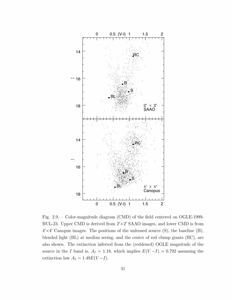
Canopus

(V-I)0 0.5 1 1.5 2

18

16

14

S

B

BL

RC

SAAO

(V-I)0 0.5 1 1.5 2

18

16

14

S

B

BL

RC

Fig. 2.9.— Color-magnitude diagram (CMD) of the field centered on OGLE-1999-

BUL-23. Upper CMD is derived from 2′×2′ SAAO images, and lower CMD is from

4′×4′ Canopus images. The positions of the unlensed source (S), the baseline (B),

blended light (BL) at median seeing, and the center of red clump giants (RC), are

also shown. The extinction inferred from the (reddened) OGLE magnitude of the

source in the I band is, AI = 1.18, which implies E(V −I) = 0.792 assuming the

extinction law AI = 1.49E(V −I).

41

If the source is at the Galactocentric distance (8 kpc), this implies that the radius

of the source is roughly 3.2 R, which is consistent with the size of a ∼ 1 M

subgiant (log g = 3.4).

Combining this result with the parameters of the best-fit model yields

θE =θ∗ρ∗

= 0.634 ± 0.043 mas , (2.14)

µ =θE

tE= 13.2 ± 0.9 µas day−1

= 22.8 ± 1.5 km s−1 kpc−1 . (2.15)

This corresponds to a projected relative velocity of 182 ± 12 km s−1 at the

Galactocentric distance, which is generally consistent with what is expected

in typical bulge/bulge or bulge/disk (source/lens) events, but inconsistent

with disk/disk lensing. Hence we conclude that the source is in the bulge.

As for properties of the lens, the projected separation of the binary lens is

1.53 ± 0.10 AU kpc−1, and the combined mass of the lens is given by

M =c2

4Gθ2ED = 0.395 ± 0.053 M

(D

8 kpc

), (2.16)

where D−1 = D−1L − D−1

S , DL is the distance to the lens, and DS is the distance to

the source.

42

2.7. Limb Darkening of the Source

We compare our determination of the linear limb-darkening coefficients to

model calculations by Claret, Dıaz-Cordoves, & Gimenez (1995) and Dıaz-Cordoves,

Claret, & Gimenez (1995). For an effective temperature of Teff = 4830±100 K and a

surface gravity of log g = 3.5, the interpolation of the V -band linear limb-darkening

coefficients, cV , of Dıaz-Cordoves et al. (1995) predicts a value cV = 0.790 ± 0.012,

very consistent with our measurement. However, for the I-band coefficient, the

prediction of Claret et al. (1995), cI = 0.578 ± 0.008, is only marginally consistent

with our measurement, at the 1.46-σ level. Adopting a slightly different gravity does

not qualitatively change this general result. Since we believe that the uncertainty

in the color of the source is larger than in the limb-darkening coefficients, we also

examine the opposite approach to the theoretical calculations – using the measured

values of limb-darkening coefficients to derive the effective temperature of the

source. If the source is a subgiant (log g 3.5) as our CMDs suggest, the measured

values of the limb-darkening coefficients are expected to be observed in stars of

the effective temperature, Teff = 4850+650−670 K for cV or Teff = 4200+390

−490 K for cI . As

before, the estimate from the V -band measurement shows a better agreement with

the measured color than the estimate from the I-band. Considering that the data

quality of I band is better than V band (the estimated uncertainty is smaller in I

than in V ), this result needs to be explained.

43

0.5 0.55 0.6 0.65 0.7

0.7

0.75

0.8

0.85

Fig. 2.10.— Comparison of linear limb-darkening coefficients. The measured value

from the best model is represented by a cross. One (solid line) and two (dotted

line) σ error ellipses are also shown. are displayed by dashed lines (log g = 3.5).

Model A is taken from Dıaz-Cordoves et al. (1995) and Claret et al. (1995), B is

from van Hamme (1993), and C is from Claret (1998b). In particular, the predicted

values in the temperature range that is consistent with our color measurements

(Teff = 4820 ± 110 K for log g = 3.0; Teff = 4830 ± 100 K for log g = 3.5; and

Teff = 4850 ± 100 K for log g = 4.0) are emphasized by thick solid lines. Model C’

is by Claret (1998b) for stars of Teff = 4850 ± 100 K for log g = 4.0. Although the

measured value of the limb-darkening coefficients alone favors this model, the model

is inconsistent with our estimation of the proper motion.

44

In Figure 2.10, we plot theoretical calculations of (cI , cV ) together with our

measured values. In addition to Dıaz-Cordoves et al. (1995) and Claret et al. (1995)

(A), we also include the calculations of linear limb-darkening coefficients by van

Hamme (1993) (B) and Claret (1998b) (C). For all three calculations, the V -band

linear coefficients are generally consistent with the measured coefficients and the

color, although van Hamme (1993) predicts a slightly smaller amount of limb

darkening than the others. On the other hand, the calculations of the I-band linear

coefficients are somewhat smaller than the measurement except for Claret (1998b)

with log g = 4.0. (However, to be consistent with a higher surface gravity while

maintaining its color, the source star should be in the disk, which is inconsistent

with our inferred proper motion.) Since cV and cI are not independent (in both

the theories and in our measurement), it is more reasonable to compare the I-

and V -band measurements to the theories simultaneously. Using the covariance

matrix of the measurement of ΓI and ΓV (see § sec:3), we derive error ellipses for

our measurements in the (cI ,cV ) plane and plot them in Figure 2.10. Formally, at

the 1-σ level, the calculations of the linear limb-darkening coefficients in any of

these models are not consistent with our measurements. In principle, one could

also constrain the most likely stellar types that are consistent with the measured

coefficients, independent of a priori information on the temperature and the gravity,

with a reference to a model. If we do this, the result suggests either that the

surface temperature is cooler than our previous estimate from the color or that

45

the source is a low-mass main sequence (log g ≥ 4.0) star. However, the resulting

constraints are not strong enough to place firm limits on the stellar type even if we

assume any of these models to be “correct.”

One possible explanation of our general result – the measured V -band

coefficients are nearly in perfect agreement with theories while the I-band

coefficients are only marginally consistent – is nonlinearity of stellar limb darkening.

Many authors have pointed out the inadequacy of the linear limb darkening in

producing a reasonably high accuracy approximation of the real stellar surface

brightness profile (Wade & Rucinski 1985; Dıaz-Cordoves & Gimenez 1992;

van Hamme 1993; Claret 1998b). Indeed, Albrow et al. (1999b) measured the

two-coefficient square-root limb darkening for a cusp-crossing microlensing event

and found that the single-coefficient model gives a marginally poorer fit to the

data. The quality of the linear parameterization has been investigated for most

theoretical limb-darkening calculations, and the results seem to support this

explanation. Van Hamme (1993) defined the quality factors (Q in his paper) for

his calculations of limb-darkening coefficients, and for 4000 K ≤ Teff ≤ 5000 K and

3.0 ≤ log g ≤ 4.0, his results indicate that the linear parameterization is a better

approximation for V band than for I band. Similarly, Claret (1998b) provided

plots of summed residuals (σ in his paper) for his fits used to derive limb-darkening

coefficients showing that the V -band linear limb-darkening has lower σ than I-band

46

and is as good as the V -band square-root limb-darkening near the temperature

range of our estimate for the source of OGLE-1999-BUL-23. In fact, Dıaz-Cordoves

et al. (1995) reported that the V -band limb darkening is closest to the linear law in

the temperature range Teff = 4500 ∼ 4750 K. In summary, the source happens to

be very close to the temperature at which the linear limb darkening is a very good

approximation in V , but is less good in I.

The actual value of the coefficient in the linear parameterization of a nonlinear

profile may vary depending on the method of calculation and sampling. In order

to determine the linear coefficients, models (A) and (C) used a least squares fit

to the theoretical (nonparametric) profile by sampling uniformly over cosϑ (see

eq. [2.5a]), while model (B) utilized the principle of total flux conservation between

parametric and nonparametric profiles. On the other hand, a fold-caustic-crossing

event samples the stellar surface brightness by convolving it with a rather

complicated magnification pattern (Gaudi & Gould 1999). Therefore, it is very

likely that neither of the above samplings and calculations is entirely suitable for

the representation of the limb-darkening measurement by microlensing unless the

real intensity profile of the star is actually the same as the assumed parametric

form (the linear parameterization, in this case). In fact, the most appropriate way

to compare the measurement to the stellar atmospheric models would be a direct fit

to the (nonparametric) theoretical profile after convolution with the magnification

47

patterns near the caustics. In the present study, this has not been done, but we

hope to make such a direct comparison in the future.

48

Chapter 3

Microlens Mass Measurement:

EROS BLG-2000-5

3.1. Introduction

Although an initial objective of microlensing experiments was to probe the

mass scale of compact subluminous objects in the Galactic halo (Paczynski 1986),

the determination of the individual lens masses was in general believed not to

be possible because the only generically measurable quantity is a degenerate

combination of the mass with lens-source relative parallax πrel and proper motion

µ (eq. [2.1]). Rather, it would be necessary to interpret the results statistically to

infer an average mass scale of the lenses from the mean timescale of the observed

events together with statistical estimates of πrel and µ. However, Gould (1992)

showed that there are additional observables that in principle can be used to break

49

the degeneracy between physical parameters and so yield a measurement of the

lens mass M . If one independently measures the projected Einstein radius rE

rE ≡√

2RSD , (3.1)

as well as the angular Einstein radius θE, then the lens mass M is obtained by

M =c2

4GrEθE

= 0.1227 M(

rE

AU

) (θE

mas

). (3.2)

Measurement of θE requires that the Einstein ring be compared with some “angular

ruler” on the plane of the sky, while to measure rE, one must compare the Einstein

ring with some “physical ruler” in the observer plane.

The only angular ruler to be used for this purpose to date is the angular radius

of the source θ∗, which can be estimated from its dereddened color and apparent

magnitude and the empirical color/surface-brightness relation (e.g., van Belle 1999).

For the subset of microlensing events in which the source passes very close to or

directly over a caustic, the finite angular extent of the source affects the lightcurve.

The source radius in units of the Einstein radius ρ∗ can then be determined through

analysis of the finite-source affected lightcurve, and thus, one can infer θE (= θ∗/ρ∗)

as well. While this idea was originally proposed for point-mass lenses, which have

pointlike caustics (Gould 1994; Nemiroff & Wickramasinghe 1994; Witt & Mao

50

1994), in practice it has been mainly used for binary lenses, which have linelike

caustics and hence much larger cross sections (Alcock et al. 1997, 2000; Albrow et

al. 1999a, 2000a; Afonso et al. 2000). In particular, one example of measurements

from the caustic-crossing binary-lens event is found in Chapter 2.

All ideas proposed to measure rE are based on the detection of parallax

effects (Refsdal 1966; Grieger, Kayser, & Refsdal 1986; Gould 1992, 1995; Gould,

Miralda-Escude, & Bahcall 1994; Hardy & Walker 1995; Holz & Wald 1996; Honma

1999): either measuring the difference in the event as observed simultaneously

from two or more locations, or observing the source from a frame that accelerates

substantially during the course of the event. Typically rE is of the order of several

AU, and so the natural scale of the parallax baseline must be ∼ 1 AU. This is

the case for the two methods proposed to measure rE: observing the event from a

satellite in solar orbit and simultaneously on Earth (Refsdal 1966; Gould 1995);

and detecting the distortion in the lightcurve due to the annual parallax effect

(Gould 1992). The latter method utilizes that the reflex of the Earth’s orbital

motion (annual parallax) induces a wobbling of the source’s passage through the

Einstein ring, which in turn perturbs the lightcurve and rE can be determined from

this perturbation. For this case, it is convenient to reexpress rE as the microlens

parallax,

πE ≡ πrel

θE

=AU

rE

. (3.3)

51

To date, this latter method is the only one by which rE has been measured (Alcock

et al. 1995; Mao 1999; Soszynski, et al. 2001; Bond et al. 2001; Smith et al. 2001;

Mao et al. 2002; Bennett et al. 2001). Unfortunately, this method requires that the

event be rather long, tE ∼> 90 days. To the extent that the Earth’s motion can be

approximated as rectilinear, it is not possible even in principle to detect this effect.

Over the relatively short timescales of typical events tE ∼ 20 days, on the other

hand, the Earth’s motion can be approximated as uniform acceleration, which can

lead to a potentially detectable asymmetry in the lightcurve (Gould et al. 1994).

However, this would yield a measurement of only a “projection” of the microlens

parallax, πE cos α′, where α′ is the angle between the direction of the lens-source

relative proper motion and that of the Earth’s acceleration vector at the peak of

the event. Hence, even if this asymmetry were detected, it would give only an

upper limit on rE. To unambiguously measure πE requires that the event last long

enough for the Earth’s acceleration vector to change substantially while the source

lies within the Einstein ring.

However, it is possible to make parallax measurements using much shorter

baselines. During a caustic crossing of a binary lens, the flux can change by several

magnitudes as the caustic transits the star. The source radius projected onto the

observer plane θ∗D can be of the order of ∼ 100 R⊕ for a main sequence star.

Hence, observers on two continents could see fluxes differing by a few percent. This

52

would again yield only one projection of the microlens parallax but by repeating

this procedure for the two caustic crossings of a single event, or by observing one

crossing from three continents, one could obtain a full measurement of parallax

(Hardy & Walker 1995; Gould & Andronov 1999). An important feature of this

approach is that it also allows to measure θE, which can be obtained from any

caustic crossing. Hence, if this method were ever applied, it would yield the

mass through equation (3.2). Unfortunately, the method requires extraordinary

cooperation from the event itself, from the observatory directors, and from the

weather. Consequently, it has not to date been successfully carried out.

It is expected that the use of the high-precision interferometric astrometry,

most notably the Space Interferometry Mission (SIM) will be the best way to

measure the individual lens mass (Paczynski 1998; Boden, Shao, & Van Buren

1998). With 10-µas level astrometry of SIM, one can directly measure πrel.

Furthermore, by monitoring the displacements in the light centroid caused by

microlensing, θE can be also directly measured (Høg, Novikov, & Polanarev 1995;

Miyamoto & Yoshii 1995; Walker 1995). Unlike most techniques mentioned earlier,

neither of these measurements requires the event to be of a special class such as

long timescale or caustic-crossing events. That is, individual lens masses can be

measured for common PSPL events.

53

Here I propose a new method to measure parallax for a subclass of caustic

crossing binaries and apply it to a binary-lens microlensing event EROS BLG-

2000-5. The method requires the event to have at least three separate well-defined

photometric peaks so that the source position can be precisely located relative to

the lens geometry at three distinct times. Two of the peaks should be caused by

caustic crossings: an entrance and an exit. It would be best for the third peak to be

a cuspy-caustic crossing, but the chance of a two fold-caustic crossing accompanied

by an additional cusp crossing is low. In the following, we investigate events where

the third peak is due either to a cusp crossing or to a generic cusp approach.

3.2. Overview

If the event has two well-observed caustic crossings, plus a well-observed “cusp

approach”, these features then provide nine “empirical parameters” – parameters

that can be measured directly from the lightcurve without appealing to a model

that depends upon a global lens geometry. They are the maximum flux Fmax, the

half-duration ∆t, and the time at the maximum tmax of each of the three peaks.

The uncertainties in the measurements of these quantities are approximately

σ(Fmax)

Fmax

∼ σ(tmax)

∆t∼ σ(∆t)

∆t∼ σph√

N= 10−3

(N

100

)−1/2 σph

1%, (3.4)

54

where σph is the mean fractional error of each of the N photometric measurements

taken over the bump. Since ∆t is generally of the order of a day, the errors in ∆t

and tmax measurements can easily be of the order of a minute or smaller. The fact

that six independent times can be measured with such precision, typically four or

five orders of magnitude smaller than the characteristic timescale of the event tE,

is what makes the parallax measurement feasible.

In principle, any localizable feature found in the lightcurve may provide similar

empirical parameters. What then makes peaks more significant as information

posts than other features such as minima or points of inflection? The answer to

this question is that the high precision measurements attainable for peaks can

rarely be achieved for empirical parameters associated with the other localizable

features, so that their merit as signature beacons is much weaker than for peaks.

For instance, minima in microlensing lightcurves typically have widths that are

ten times greater than peaks have (and by definition less flux as well). From

equation (3.4), σ(t) ∝ (∆t/F )1/2, so that it is substantially more difficult to localize

minima than peaks. Here, we assume Poisson noise (σph =√

F/F ), and the same

sampling frequency (i.e., N ∝ ∆t). Points of inflection are even more difficult to

localize than minima.

Ordinarily, under the approximation that the lens-source relative motion is

rectilinear, to specify a binary-lens lightcurve requires a set of seven global (or

55

geometric) parameters (d, q, tE, t0, α, u0, ρ∗). However, since the actual motion is

not rectilinear, these seven parameters will not be adequate to describe the event

with very high precision, and in particular, subtle inconsistencies will be introduced

among the nine precisely measured quantities mentioned earlier. We now show how

these inconsistencies can lead to a parallax measurement.

3.3. Measurement of Parallax from Triple-Peak

Events

In practice, the parallax will be measured by multidimensional fitting and

subsequent χ2 minimization. However, it is instructive for two reasons to identify

in a systematic way the features of the event that permit πE to be measured. First,

this enables one to predict when an event will have a measurable πE. Second,

there are technical difficulties associated with χ2 minimization, and these can be

ameliorated if the model parameterization is modified to reflect the underlying

physics (Albrow et al. 1999c).

To understand how πE is measured, we first show how some of the nine

empirical parameters are related to one another in the absence of parallax, i.e.,

πE = 0. We will initially assume that the lens geometry (d,q) and the fluxes Fs and

Fb are known a priori. Then, at the peak of the cusp approach tmax,ca, the source

56

position within the Einstein ring uca can be determined very precisely from the

precise measurements of tmax,ca and Fmax,ca. That is, at this time tmax,ca, the source

must be somewhere along the cusp-approach ridge line, and its position on that

line is determined from the inferred magnification A = (Fmax,ca − Fb)/Fs.

Now consider the angles at which the source crosses each caustic line, φ1 and

φ2. The half-duration of a caustic crossing is given by ∆tcc = tEρ∗ csc φ. If this

motion is assumed to be rectilinear, then tE becomes a well-defined quantity over

the whole duration of the event, and thus,

csc φ2

csc φ1

=∆tcc,2∆tcc,1

. (3.5)

The source trajectory is then the straight line that passes through uca and has

caustic-crossing angles that satisfy equation (3.5). From that equation, this angle

can be determined with a precision of

σ(α) =1

| cot φ2 − cot φ1|

[σ(∆tcc,2)

∆tcc,2

]2

+

[σ(∆tcc,1)

∆tcc,1

]2

1/2

, (3.6)

which can be estimated using equation (3.4).

Next, we turn to the times of the two caustic crossings t0,cc,1 and t0,cc,2, at

which the center of the source lies on the caustic lines. These are not the same as

the times of peak flux tmax,cc,1 and tmax,cc,2, but they can be determined to the same

precision (see eq. [3.4]) and are more convenient to work with. Let ucc,1 and ucc,2

57

be the positions in the Einstein ring of the two caustic crossings. For rectilinear

motion, these satisfy the vector equation,

ucc,2 − ucc,1

t0,cc,2 − t0,cc,1

=uca − ucc,1

tmax,ca − t0,cc,1

= µE . (3.7)

Here µE ≡ µ/θE so that the magnitude of the one side of the equation is the

same as t−1E . However, if the acceleration due to the Earth’s orbital motion is not

negligible, equation (3.7) will not in general be satisfied. This can be quantified

in terms of δt2, the difference between the measured value of t0,cc,2 and the one

that would be predicted from the other measured parameters on the basis of

equation (3.7),

δt2 ≡ (t0,cc,2 − t0,cc,1) − |ucc,2 − ucc,1||uca − ucc,1| (tmax,ca − t0,cc,1) . (3.8)

To evaluate the relation between δt2 and πE, we make the approximation that the

Earth’s acceleration vector projected on the sky a⊕,⊥ is constant for the duration

of the caustic crossings and cusp approach. We first note that the magnitude of

this acceleration is related to the parallax by

|a⊕,⊥|rE

= πE| sin ψ|(

Ω

r⊕/AU

)2

, (3.9)

where ψ is the angle between the lines of sight toward the Sun and the event from

the Earth, r⊕ is the distance between the Sun and the Earth, during the caustic

58

crossings, and Ω = 2π yr−1. Then, after some algebra, we find

δt2t3 − t2

=| sin ψ|tE

2

(Ω

r⊕/AU

)2

×−πE,‖ (t2−t1) + πE,⊥ [(t3−t2) cot φ2 − (t3−t1) cot φ1]

, (3.10)

where we have used the simplified notations, t0,cc,i → ti and tmax,ca → t3 and

introduce a two-dimensional vector πE whose magnitude is πE and whose direction

is that of µ. Here πE,‖ and πE,⊥ are the components of πE parallel and perpendicular

to a⊕,⊥. Hence, by measuring δt2 one can determine a particular projection of πE

whose components are given by equation (3.10).

However, since πE is a two-dimensional vector, measurements of two

independent components are required for the complete determination of πE. A

second constraint is available from the width of the cusp approach ∆tca. We define

δ ln ∆tca in analogy to δt2 and after some more algebra we find

δ ln ∆tca =| sin ψ|tE

cot φ2 − cot φ1

(Ω

r⊕/AU

)2

×πE,‖ [(t3−t2) cotφ1 + (t2−t1) cotφ3 − (t3−t1) cotφ2]

+ πE,⊥ [(t3−t1) cotφ3 cotφ1 − (t3−t2) cotφ3 cotφ2 − (t2−t1) cotφ2 cotφ1] .

(3.11)

Measurement of δ ln ∆tca therefore gives another projection of πE. Furthermore, it

is possible to obtain a third constraint on πE from the behavior of the lightcurve

59

after the source has left the caustic, but while it still remains within the Einstein

ring. For rectilinear motion, the Einstein time scale is well determined (see

eq. [3.7]). If the latetime lightcurve drops off faster or slower than indicated by this

timescale, it implies that the Earth’s acceleration vector has a component aligned

with the direction of lens-source relative motion. The effect is similar to the one

identified by Gould et al. (1994) but can be measured more easily because both tE

and t0 are determined very precisely from the lightcurve around the caustic-crossing

region.

The relative orientation of these three constraints depends on the details of the

lens geometry. In principle, they could all be roughly parallel, but this is unlikely;

in general, it should be possible to combine the three projections to measure both

components of πE. If the event is sufficiently long (typically tE ∼> 60 days) that the

Earth moves ∼> 1 radian during an Einstein timescale, then the latetime behavior

of the lightcurve will give information about both components of πE. In this case

there would be the fourth constraint.

The exact expression for the errors in the components of πE obtained from

the first two constraints can be derived from equations (3.10) and (3.11), but these

are extremely complicated and, for that reason not very interesting. However,

reasonable estimates of these errors can be made as follows. First, we note that the

error from applying the δt2 constraint is dominated by the problem of determining

60

the change in α from the parallax to the nonparallax case. The error in the

measurement of α is given by equation (3.6). On the other hand, the change in α

(chosen for definiteness to be the angle at the time of the cusp approach) is given

by

(cot φ2 − cot φ1)δα =2δt2

t3 − t2. (3.12)

Hence, the fractional error in πE,δt2 , the projection of πE measured by this

constraint, is of the order of

σ(πE,δt2)

πE,δt2

∼ σ(α)

δα∼ N−1/2 σph

| sin ψ|Ω2(t2 − t1)tEπE

, (3.13)

where we have made use of equations (3.4) and (3.6). For typical bulge

parameters, | sin ψ| ∼ 0.2 and πE ∼ 0.1, and with good photometric

coverage of the caustic crossings, N−1/2σph ∼ 10−3, the fractional error is

∼ 0.17 × (tE/50 days)−1 × [(t2 − t1)/20 days]−1 and hence πE,δt2 should plausibly

be measurable. For the other constraint one finds similar expressions.

We now relax our assumption that d, q, Fs, and Fb are known a priori.

Actually, if (d,q) are known, Fs and Fb can be easily determined from, for example,

the baseline flux Fs + Fb, and the minimum flux observed inside the caustic

AminFs + Fb. Here Amin is the magnification at minimum that, for a fixed (d,q), is

virtually independent of the minor adjustments to the trajectory due to parallax.

61

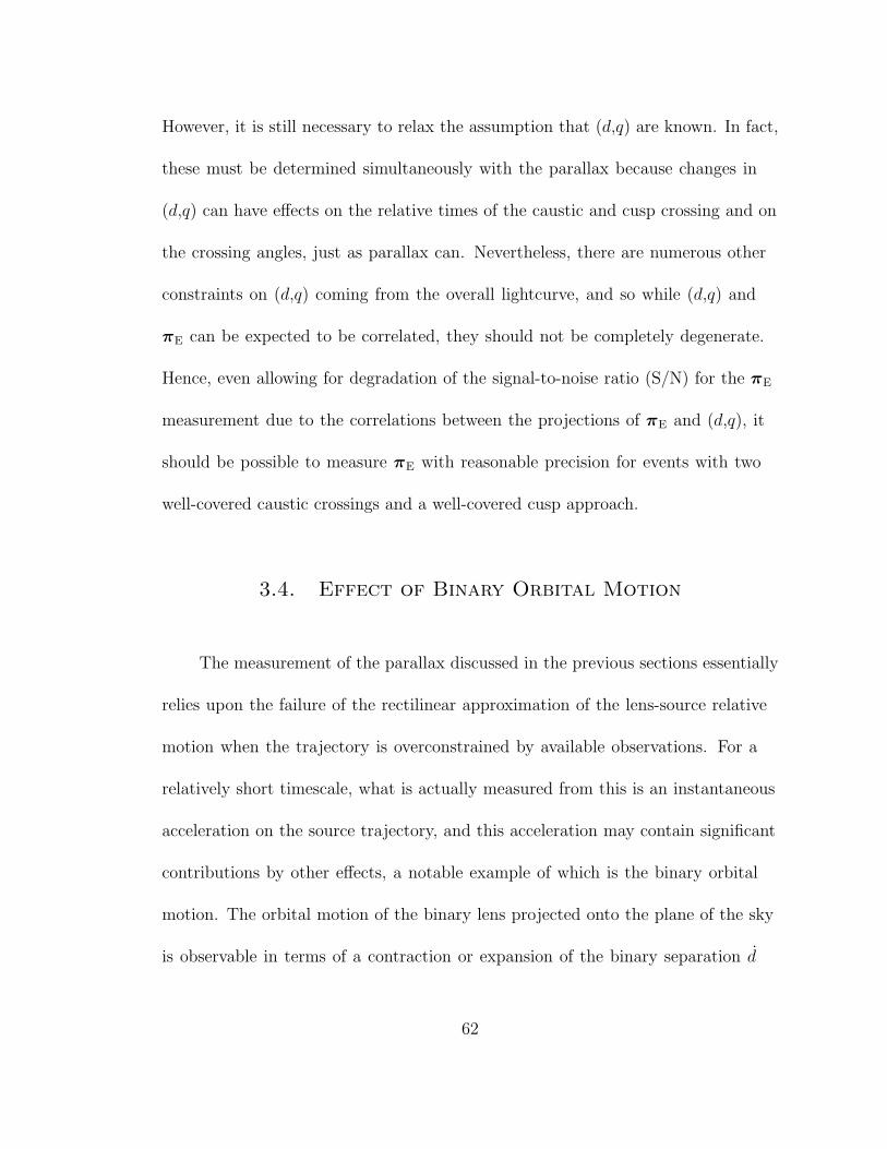
However, it is still necessary to relax the assumption that (d,q) are known. In fact,

these must be determined simultaneously with the parallax because changes in

(d,q) can have effects on the relative times of the caustic and cusp crossing and on

the crossing angles, just as parallax can. Nevertheless, there are numerous other

constraints on (d,q) coming from the overall lightcurve, and so while (d,q) and

πE can be expected to be correlated, they should not be completely degenerate.

Hence, even allowing for degradation of the signal-to-noise ratio (S/N) for the πE

measurement due to the correlations between the projections of πE and (d,q), it

should be possible to measure πE with reasonable precision for events with two

well-covered caustic crossings and a well-covered cusp approach.

3.4. Effect of Binary Orbital Motion

The measurement of the parallax discussed in the previous sections essentially

relies upon the failure of the rectilinear approximation of the lens-source relative

motion when the trajectory is overconstrained by available observations. For a

relatively short timescale, what is actually measured from this is an instantaneous

acceleration on the source trajectory, and this acceleration may contain significant

contributions by other effects, a notable example of which is the binary orbital

motion. The orbital motion of the binary lens projected onto the plane of the sky

is observable in terms of a contraction or expansion of the binary separation d

62

and the lateral rotation of the binary axis with respect to the fixed direction on

the sky ω. The apparent observable result of the latter effect may heuristically be

understood as a centripetal acceleration ∼ ucω2 on the source motion relative to

the (static) lens system, where uc is the angular extent of the caustic in units of

the Einstein ring. For a face-on circular binary orbit observed at the ecliptic pole,

the ratio of the Earth’s acceleration to the projected acceleration due to the binary

orbital motion is then

a⊕abin

=πE

uc

(P

yr

)2

. (3.14)

Thus, depending on these parameters, either parallax or binary orbital motion

could dominate. In addition for the general case, both the Earth and binary

acceleration would be reduced by possibly very different projection factors (while

the projection factor for the binary orbital motion is from the orbital inclination of

the binary, the parallactic projection is due to the angle between the direction to

the ecliptic pole and the line of sight to the event). Although the effect of d is, in

general, not expressible analytically, one can expect it to be of a similar order of

magnitude to that of ω.

An unambiguous determination of the parallax therefore requires the

measurement of the acceleration at least at two different times or not less than four

independent constraints on the projection of the acceleration at different times.

63

We argued above that there are generically at least three constraints for the types

of events under discussion and that there is a fourth constraint for sufficiently

long events. In this latter case, parallax can be unambiguously discriminated from

projected orbital motion. However, even when the event is short, so that there are

only three constraints, it may still be feasible to measure the parallax. We first

note that the orbital motion cannot significantly affect the latetime lightcurve –

i.e., tE is not influenced by the orbital motion – for it does not affect separations

between the source and the binary center of mass. Hence, if one component of πE

is measured from the latetime lightcurve, it may be possible using equation (3.14)

and Kepler’s Third Law to show that parallax is more important than projected

orbital motion, in which case the caustic crossings can be used to determine the

full parallax πE.

In brief, there is good reason to hope that events with three well-defined

bumps can yield parallax measurements and, hence, mass measurements from the

combination with the measurement of the angular Einstein radius. Whether this

will be possible for any particular such event can only be determined by detailed

modeling.

64

3.5. EROS BLG-2000-5

So far, we have argued that πE is measurable for a caustic-crossing binary

event exhibiting a well-observed peak caused by a cusp approach in addition to the

two usual caustic crossings. Here we provide the application of the method to the

actual triple-peak caustic-crossing binary microlensing event EROS BLG-2000-5.

In addition, the event has a relatively long time scale (tE ∼ 100 days), which is

generally favorable for the measurement of πE.

In fact, EROS BLG-2000-5 features many unique characteristics not only in

the intrinsic nature of the event but also in the observations of it. These include a

moderately well-covered first caustic crossing (entrance), a timely prediction – of

not only the timing but also the duration – of the second caustic crossing (exit),

the unprecedented four-day length of the second crossing, and two time-series of

spectral observations of the source during the second crossing (Albrow et al. 2001b;

Castro et al. 2001). To fully understand and utilize this wealth of information,

however, requires detailed quantitative modeling of the event. In the rest of this

chapter, we focus on the modeling of the geometry of the event based on the

photometric observations made by the PLANET collaboration and find that both

parallax and projected binary orbital motion are required to successfully model the

lightcurve. Furthermore, as is usual for caustic-crossing events, we also measure

the angular Einstein radius from the finite source effect during caustic crossings

65

and the source angular size derived from the source position in the CMD. Hence,

this is the first event for which both rE and θE are measured simultaneously and so

for which the lens mass is unambiguously measured.

3.5.1. Data

On 2000 May 5, the Experience pour la Recherche d’Objets Sombres (EROS)1

collaboration issued an alert that EROS BLG-2000-5 was a probable microlensing

event (RA = 17h53m11.s5, Dec = −3055′35′′; l = 359.14, b = −2.43). On 2000

June 8, the Microlensing Planet Search (MPS)2 collaboration issued an anomaly

alert, saying that the source had brightened by 0.5 mag from the previous night

and had continued to brighten by 0.1 mag in 40 minutes. PLANET intensified

its observations immediately, and has been continuing to monitor the event up to

the 2001 season. Observations for PLANET were made from four telescopes: the

Canopus 1 m near Hobart, Tasmania, Australia; the Perth/Lowell 0.6 m at Perth

Observatory, Bickley, Western Australia, Australia; the Elizabeth 1 m at SAAO,

Sutherland, South Africa; and the YALO 1 m at CTIO, La Serena, Chile. Data

were taken in V (except Perth), I (all four sites), and H (SAAO and YALO) bands.

For the present study, we make use primarily of the I band data. That is, we fit for

the model using only I band data, while the V band data are used (together with

1 http://www-dapnia.cea.fr/Spp/Experiences/EROS/alertes.html2 http://bustard.phys.nd.edu/MPS/

66

the I data) only to determine the position of the source on CMD (see § 3.8). The

lightcurve (Fig. 3.1) exhibits two peaks that have the characteristic forms of an

entrance (A) and exit (B) caustic crossing (Schneider, Ehlers, & Falco 1992, also

see fig. 1 of Gould & Andronov 1999) immediately followed by a third peak (C)

which is caused by the passage of the source close to a cusp.

The data have been reduced in a usual way and the photometry on them has

been performed by point spread function (PSF) fitting using DoPHOT (Schechter

et al. 1993). The relative photometric scaling between the different telescopes is

determined as part of the fit to the lightcurve which includes the independent

determinations of the source and the background fluxes at each telescope. We find,

as was the case for several previous events, that due to the crowdedness of the field,

the moderate seeing conditions, and possibly some other unidentified systematics,

the amount of blended light entering the PSF is affected by seeing, and that the

formal errors reported by DoPHOT tend to underestimate the actual photometric

uncertainties. We tackle these problems by incorporating a linear seeing correction

for the background flux and rescaling the error bars to force the reduced χ2 of our

best model to unity. For details of these procedures, refer Chapter 2 as well as

Albrow et al. (2000a,b) and Gaudi et al. (2002).

We also analyze the data by difference imaging, mostly using ISIS (Alard

& Lupton 1998; Alard 2000). We compare the scatter of the photometry on

67

Fig. 3.1.— PLANET I-band lightcurve of EROS BLG-2000-5 (the 2000 season

only). Only the data points used for the analysis (“cleaned high-quality” subset; see

§ 3.5.1) are plotted. Data shown are from SAAO (circles), Canopus (triangles),

YALO (squares), and Perth (inverted triangles). All data points have been

deblended using the fit result – also accounting for the seeing correction – and

transformed to the standard I magnitude; I = Is − 2.5 log[(F (t) − Fb)/Fs]. The

calibrated source magnitude (Is = 16.602) is shown as a dotted line. The three

bumps in the lightcurve and the corresponding positions relative to the microlens

geometry are also indicated.

68

the difference images to that of the direct PSF fit photometry by deriving the

normalized-summed squares of the S/Ns:

Q ≡ ∑i

(FsAi

σi

)2

=N

χ2

∑i

(FsAi

σi

)2

, (3.15)

where Fs is the source flux derived from the model, Ai is the magnification predicted

by the model for the data point, σi and σi are the photometric uncertainty (in flux)

for individual data before and after rescaling the error bars [i.e., σi = σi(χ2/N)1/2],

and N is the number of the data points. Strictly speaking, Q defined as in

equation (3.15) is model-dependent, but if the data sets to be compared do not

differ with one another in systematic ways (and the chosen model is close enough to

the real one), Q can be used as a proxy for the relative statistical weight given by

the data set without notable biases. We find that difference imaging significantly

improves the stability of the photometry for the data from Canopus and Perth,

but it somewhat worsens the photometry for the data from SAAO and YALO. We

suspect that the result is related to the overall seeing condition for the specific site,

but a definite conclusion will require more detailed study and would be beyond

the scope of the current research. We hope to be able to further improve the

photometry on difference images in the future, but for the current analysis, we

choose to use the data set with the better Q so that only for Canopus and Perth

data sets, we replace the result of the direct PSF photometry with the difference

imaging analysis result.

69

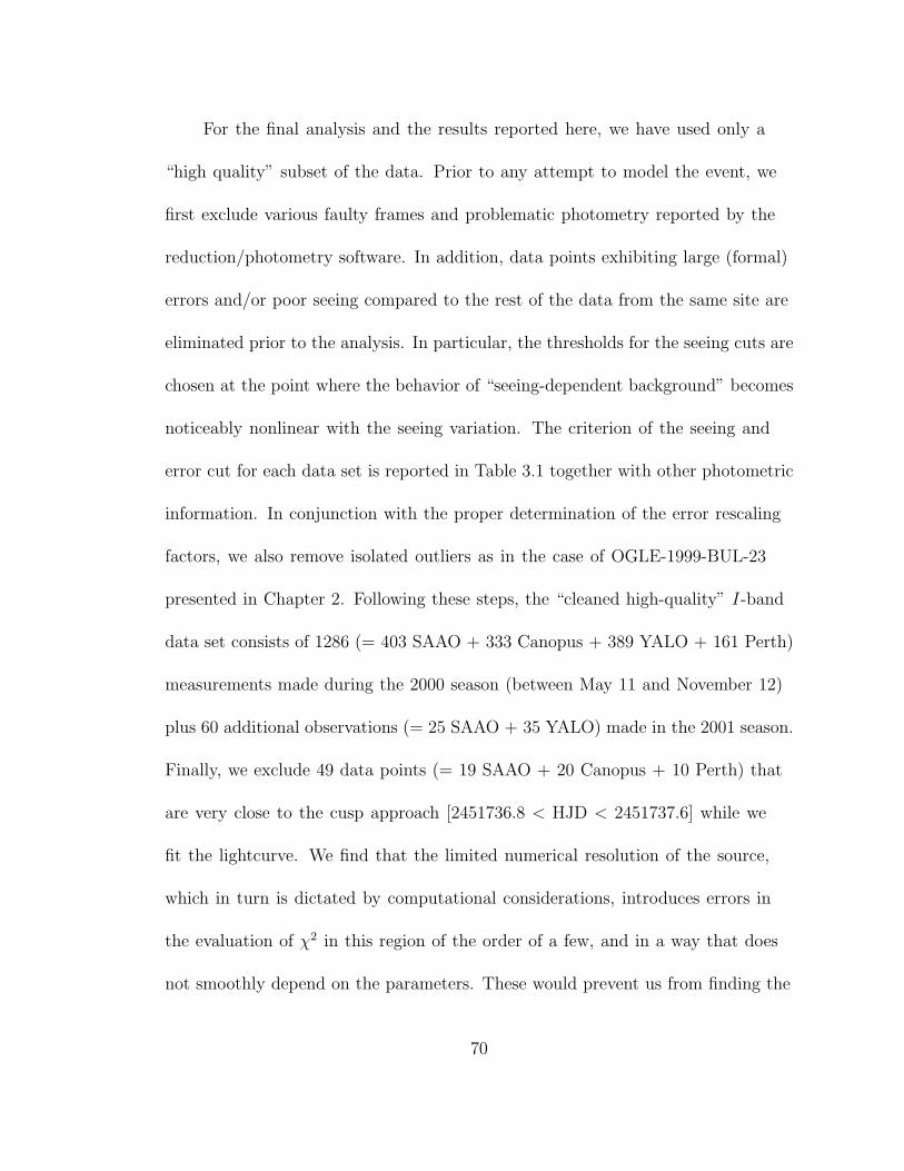
For the final analysis and the results reported here, we have used only a

“high quality” subset of the data. Prior to any attempt to model the event, we

first exclude various faulty frames and problematic photometry reported by the

reduction/photometry software. In addition, data points exhibiting large (formal)

errors and/or poor seeing compared to the rest of the data from the same site are

eliminated prior to the analysis. In particular, the thresholds for the seeing cuts are

chosen at the point where the behavior of “seeing-dependent background” becomes

noticeably nonlinear with the seeing variation. The criterion of the seeing and

error cut for each data set is reported in Table 3.1 together with other photometric

information. In conjunction with the proper determination of the error rescaling

factors, we also remove isolated outliers as in the case of OGLE-1999-BUL-23

presented in Chapter 2. Following these steps, the “cleaned high-quality” I-band

data set consists of 1286 (= 403 SAAO + 333 Canopus + 389 YALO + 161 Perth)

measurements made during the 2000 season (between May 11 and November 12)

plus 60 additional observations (= 25 SAAO + 35 YALO) made in the 2001 season.

Finally, we exclude 49 data points (= 19 SAAO + 20 Canopus + 10 Perth) that

are very close to the cusp approach [2451736.8 < HJD < 2451737.6] while we

fit the lightcurve. We find that the limited numerical resolution of the source,

which in turn is dictated by computational considerations, introduces errors in

the evaluation of χ2 in this region of the order of a few, and in a way that does

not smoothly depend on the parameters. These would prevent us from finding the

70

true minimum, or properly evaluating the statistical errors. However, for the final

model, we evaluate the predicted fluxes and residuals for these points. As we show

in § 3.7, these residuals do not differ qualitatively from other residuals to the fit.

3.6. Parameterization

While to specify the lightcurve of a static binary event with a rectilinear

source trajectory requires a set of seven geometric parameters (d, q, tE, t0, α,

u0, ρ∗), to generally incorporate the annual parallax and the projection of binary

orbital motion into the model, one needs four additional parameters. However,

their inclusion, especially of the parallax parameters, is not a trivial procedure,

since the natural coordinate basis for the description of the parallax is the ecliptic

system while the binary magnification pattern possesses its own preferred direction,

i.e., the binary axis. In the following, we establish a consistent system to describe

the complete set of the eleven geometric parameters.

71

3.6.1. Description of Geometry

First, we focus on the description of parallax. On the plane of the sky, the

angular positions of the lens and the source (seen from the center of the Earth) are

expressed generally by,

ϕS(t) = ϕS,c + (t − tc)µS + πSς(t) , (3.16a)

ϕL(t) = ϕL,c + (t − tc)µL + πLς(t) . (3.16b)

Here ϕS,c and ϕL,c are the positions of the lens and the source at some reference

time, t = tc, as they would be observed from the Sun, µS and µL are the

(heliocentric) proper motion of the source and the lens, πS and πL are the annual

trigonometric parallax, and ς(t) is the Sun’s position vector with respect to the

Earth, projected onto the plane of the sky and normalized by an astronomical

unit (see Appendix B). At any given time, t, ς(t) is completely determined with

respect to an ecliptic coordinate basis, once the event’s (ecliptic) coordinates are

known. For example, in the case of EROS BLG-2000-5 (λ = 268.53, β = −7.50),

ς = (0, r⊕ sin β) at approximately 2000 June 19, where r⊕ is the distance between

the Sun and the Earth at this time in astronomical units (r⊕ = 1.016). Then, the

angular separation vector between the source and the lens in units of θE becomes

u(t) ≡ ϕS − ϕL

θE

= υ + (t − tc)µE − πEς(t) , (3.17)

72

where υ ≡ (ϕS,c − ϕL,c)/θE. Although equation (3.17) is the most natural form

of expression for the parallax-affected trajectory, it is convenient to reexpress

equation (3.17) as the sum of the (geocentric) rectilinear motion at the reference

time and the parallactic deviations. In order to do this, we evaluate u and u at

t = tc,

utc ≡ u(tc) = υ − πEς tc , (3.18a)

utc ≡ u(tc) = µE − πEς tc , (3.18b)

where ς tc ≡ ς(tc) and ς tc ≡ ς(tc). Solving equations (3.18) for µE and υ and

substituting them into equation (3.17), one obtains

u(t) = utc + (t − tc)utc − πEDP , (3.19)

where DP ≡ ς(t) − ς tc − (t − tc)ς tc is the parallactic deviation. Note that

DP (ς tc/2)(t− tc)2 for t ∼ tc, i.e., on relatively short time scales, the effect of the

parallax is equivalent to a uniform acceleration of −πEς tc . Equation (3.19) is true

in general for any microlensing event including PSPL events.

Next, we introduce the binary lens system. Whereas the parallax-affected

trajectory (eq. [3.19]) is most naturally described in the ecliptic coordinate system,

the magnification pattern of the binary lens is specified with respect to the binary

73

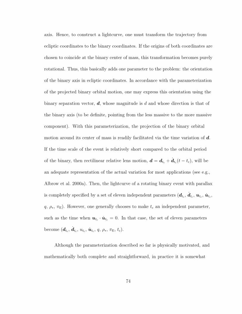
axis. Hence, to construct a lightcurve, one must transform the trajectory from

ecliptic coordinates to the binary coordinates. If the origins of both coordinates are

chosen to coincide at the binary center of mass, this transformation becomes purely

rotational. Thus, this basically adds one parameter to the problem: the orientation

of the binary axis in ecliptic coordinates. In accordance with the parameterization

of the projected binary orbital motion, one may express this orientation using the

binary separation vector, d, whose magnitude is d and whose direction is that of

the binary axis (to be definite, pointing from the less massive to the more massive

component). With this parameterization, the projection of the binary orbital

motion around its center of mass is readily facilitated via the time variation of d.

If the time scale of the event is relatively short compared to the orbital period

of the binary, then rectilinear relative lens motion, d = dtc + dtc(t − tc), will be

an adequate representation of the actual variation for most applications (see e.g.,

Albrow et al. 2000a). Then, the lightcurve of a rotating binary event with parallax

is completely specified by a set of eleven independent parameters (dtc , dtc , utc , utc ,

q, ρ∗, πE). However, one generally chooses to make tc an independent parameter,

such as the time when utc · utc = 0. In that case, the set of eleven parameters

become (dtc , dtc , utc , utc , q, ρ∗, πE, tc).

Although the parameterization described so far is physically motivated, and

mathematically both complete and straightforward, in practice it is somewhat

74

cumbersome to implement into the actual fit. Therefore, we reformulate the above

parameterization for computational purposes. For the analysis of EROS BLG-

2000-5, we first choose the reference time tc as the time of the closest approach

of the source to the cusp, and rotate the coordinate system so that the whole

geometry is expressed relative to the direction of dtc , i.e., the binary axis at

time tc (see Fig. 3.2). We define the impact parameter for the cusp approach, uc

(≡ |utc − ucusp|), and set uc > 0 when the cusp is on the righthand side of the

moving source. Then, utc is specified by t′E (≡ |utc|−1), the instantaneous Einstein

timescale at time tc, and by α′, the orientation angle of utc with respect to dtc .

In addition, we express dtc in a polar-coordinate form and use the approximation

that both the radial component, d, and tangential component, ω, are constant.

Under this parameterization, d corresponds to the rate of expansion (d > 0) or

contraction (d < 0) of the projected binary separation while ω is the angular

velocity of the projected binary-axis rotation on the plane of the sky. Finally,

we define the microlens parallax vector, πE, whose magnitude is πE and whose

direction is toward ecliptic west (decreasing ecliptic longitude). In the actual fit,

πE,‖ and πE,⊥, the two projections of πE along and normal to dtc , are used as

independent parameters. Table 3.2 summarizes the transformation from the set

of fit parameters (dtc , q, α′, uc, t

′E, tc, ρ∗, πE,‖, πE,⊥, d, ω) to the set of the physical

parameters (dtc , dtc , utc , utc , q, ρ∗, πE, tc).

75

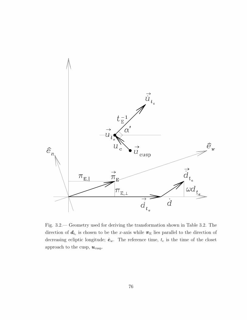
Fig. 3.2.— Geometry used for deriving the transformation shown in Table 3.2. The

direction of dtc is chosen to be the x-axis while πE lies parallel to the direction of

decreasing ecliptic longitude; ew. The reference time, tc is the time of the closet

approach to the cusp, ucusp.

76

3.6.2. The Choice of Fit Parameters

Judged by the number of fitting parameters alone, EROS BLG-2000-5

is by far the most complex event ever analyzed: compared to the runner-up,

MACHO 99-BLG-47 (Bennett et al. 1999; Albrow et al. 2000a), it has two more

geometric parameters and one more limb-darkening parameter. As a direct result,

the path toward choosing a modeling procedure was substantially more tortuous

than usual. We therefore believe that it is important to document this path, at

least in outline, in order to aid in the modeling of future events.

As stated in § 3.6, the seven standard parameters for binary events are

(d, q, tE, t0, α, u0, ρ∗). Immediately following the first caustic crossing, we fit

this crossing to five empirical parameters, including tcc,1 and ∆t1, the time and

half-duration of the first crossing (see § 2.4.1). We then changed our choice of

parameters (t0, ρ∗) → (tcc,1, ∆t1) according to the prescription of Albrow et al.

(1999c), effectively cutting the search space down from seven to five dimensions,

and speeding up the search accordingly. This permitted us to accurately predict in

real time not only the time, but also the (4-day) duration of the second crossing

which in turn allowed two groups to obtain large-telescope spectra of the crossing

(Albrow et al. 2001b; Castro et al. 2001). This was the first prediction of the

duration of a caustic crossing.

77

Why is the substitution (t0, ρ∗) → (tcc,1, ∆t1) critical? Both tcc,1 and ∆t1 are

determined from the data with a precision ∼ 10−3 day ∼ 10−5 tE. Hence, if any of

the parameters, α, u0, t0, ρ∗, are changed individually by 10−4 (subsequent changes

of tcc,1 and ∆t1 by 10−4 tE), this will lead to an increase ∆χ2 ∼ 100. As a result,

even very modest movements in parameter space must be carefully choreographed

to find a downhill direction on the χ2 hypersurface. By making (tcc,1, ∆t1) two of

the parameters and constraining them to very small steps consistent with their

statistical errors, one in effect automatically enforces this choreography.

In all the work reported here, we searched for χ2 minima at fixed (d,q), and

repeated this procedure over a (d,q) grid. We found for this event (as we have

found for others) that regardless of what minimization technique we apply, if we

search (d,q) space simultaneously with the other parameters, then either we do not

find the true χ2 minimum or the search requires prohibitive amounts of time.

Following the second crossing, we added a linear limb-darkening (LD)

parameter, but otherwise continued with the same parameterization. We found

that the fitting process was then enormously slowed down because small changes

α, u0, or tE led to large changes in tcc,2 and ∆t2 (the second crossing time and

half-duration), whereas these quantities were directly fixed by the data. We

therefore changed parameters (α, u0, tE) → (tcc,2, ∆t2, taxis), where taxis is the time

the source crossed the cusp axis. Hence, all five of the non-(d, q) parameters were

78

fixed more-or-less directly by the data, which greatly improved the speed of our

parameter search. We thus quickly found the χ2 minimum for this (7+1)-parameter

– seven geometry plus one limb-darkening – space. (Note that the LD parameter,

like the source flux, the background flux, and the seeing correlation, is determined

by linear fitting after each set of other parameters is chosen. Hence, it exacts

essentially zero computational cost. We therefore track it separately.)

Since the lightcurve showed systematic residuals of several percent (compared

to daily-averaged photometry errors 1%), we were compelled to introduce more

parameters. We first added two parallax parameters; the magnitude πE and its

relative orientation with respect to the binary, yielding a (9+1)-parameter fit.

Since five of the nine geometrical parameters remained empirical, this procedure

also converged quickly. However, while χ2 had fallen by several hundred (indicating

a very significant detection of parallax), the problem of systematic residuals was

not qualitatively ameliorated. This created something of a crisis. We realized that

further improvements would be possible if we allowed for binary orbital motion.

Lacking apparent alternatives, we went ahead and introduced projected binary

orbital motion. This led to radical changes in our now (11+1)-parameterization.

Allowing two dimensions of binary motion meant that both the orientation and

the size of the binary separation could change. The latter induced changes in both

the size and shape of the caustic, and so made it essentially impossible to define

79

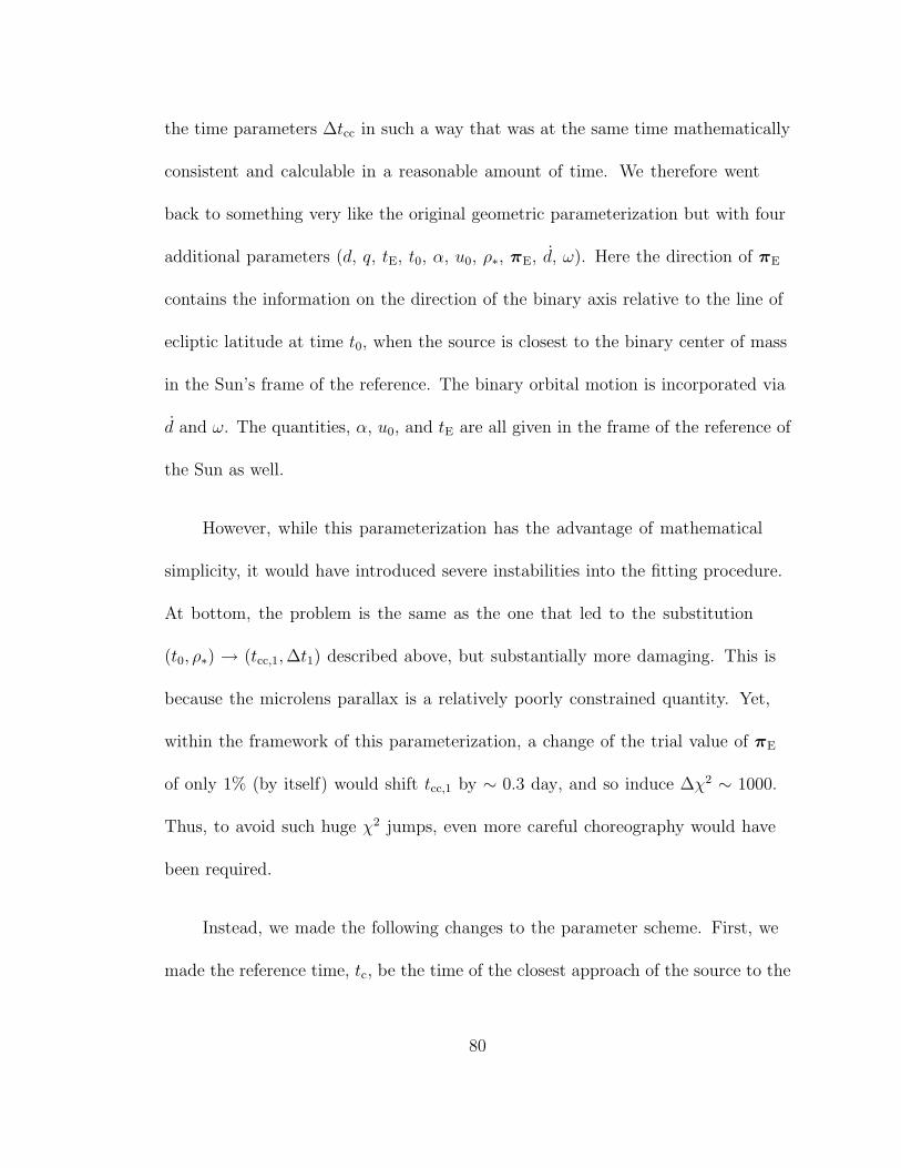
the time parameters ∆tcc in such a way that was at the same time mathematically

consistent and calculable in a reasonable amount of time. We therefore went

back to something very like the original geometric parameterization but with four

additional parameters (d, q, tE, t0, α, u0, ρ∗, πE, d, ω). Here the direction of πE

contains the information on the direction of the binary axis relative to the line of

ecliptic latitude at time t0, when the source is closest to the binary center of mass

in the Sun’s frame of the reference. The binary orbital motion is incorporated via

d and ω. The quantities, α, u0, and tE are all given in the frame of the reference of

the Sun as well.

However, while this parameterization has the advantage of mathematical

simplicity, it would have introduced severe instabilities into the fitting procedure.

At bottom, the problem is the same as the one that led to the substitution

(t0, ρ∗) → (tcc,1, ∆t1) described above, but substantially more damaging. This is

because the microlens parallax is a relatively poorly constrained quantity. Yet,

within the framework of this parameterization, a change of the trial value of πE

of only 1% (by itself) would shift tcc,1 by ∼ 0.3 day, and so induce ∆χ2 ∼ 1000.

Thus, to avoid such huge χ2 jumps, even more careful choreography would have

been required.

Instead, we made the following changes to the parameter scheme. First, we

made the reference time, tc, be the time of the closest approach of the source to the

80

cusp, rather than the closest approach to the center of mass. Second, we adopted,

for the frame of reference, the frame of the Earth at tc rather than the frame of the

Sun. Our final choice of parameters is (dtc , q, t′E, tc, α′, uc, ρ∗, πE, d, ω), where uc

is the impact parameter relative to the cusp and α′ and t′E are evaluated at tc and

in the frame of reference of the Earth at the time. The change of reference frame

is responsible for the form of the parallax deviation given in equation (3.19), but

from a practical point of view it is very helpful so that the non-parallax parameters

do not change very much when the parallax is changed: in particular they are

similar to the solution without parallax (i.e., πE ≡ 0). The particular choice of the

reference time tc is useful because most of the “action” of the event happens close

to this time, either during the cusp approach itself, or during the second caustic

crossing a week previously. Hence, both tc and uc are relatively well fixed by the

data, while the angle α is also relatively well fixed since it is strongly constrained

by the cusp approach and second crossing. As a consequence, we are able to find

relatively robust minima for each (d, q) grid point in about a single day of computer

time, which is quite adequate to reach a global minimum.

Unfortunately, the (11+1)-parameterization failed to qualitatively lessen the

problem of systematic residuals. We then recognized that more LD freedom was

required, and so added a square-root LD parameter in addition to the linear

one. This reduced the systematic residuals to < 1%. As a result, we fit limb

81

darkening with a two-parameter form so that the final fit we adopted is an

(11+2)-parameterization fit.

3.6.3. Terrestrial Baseline Parallax

In general, the Earth’s spin adds a tiny daily wobble of order ∼ R⊕/rE

(eq. [C.3]), where R⊕ is the Earth’s radius, to the source’s relative position

seen from the center of the Earth as expressed in equation (3.17). Since

R⊕ = 4.26 × 10−5 AU, this effect is negligible except when the spatial gradient

over the magnification map is very large, e.g., caustic crossings or extreme cusp

approaches. Even for those cases, only the instantaneous offsets are usually what

matters because the source crosses over the region of extreme gradient with a time

scale typically smaller than a day. Hence, unless the coverage of the crossing from

two widely separated observers significantly overlaps, the effect has been in general

ignored when one models microlensing lightcurves.

However, in case of EROS BLG-2000-5, the second caustic crossing lasted four

days, and therefore daily modulations of magnifications due to the Earth’s rotation,

offset according to the geographic position of each observatory, may become

important, depending on the actual magnitude of the effect (See also Honma 1999

for a similar discussion on the short time scale magnification modulation observed

from an Earth-orbiting satellite). Hardy & Walker (1995) and Gould & Andronov

82

(1999) investigated effects of the terrestrial baseline parallax, for fold-caustic

crossing microlensing events mainly focused on the instantaneous offsets due to the

separation between observers. They argued that the timing difference of the trailing

limb crossing for observations made from two different continents could be of the

order of tens of seconds to a minute (Hardy & Walker 1995) and the magnifications

near the end of exit-type caustic crossings could differ by as much as a few percent

(Gould & Andronov 1999). Suppose that φ2 is the angle at which the source

crosses the caustic, Amax is the magnification at the peak of the crossing, and Acc is

the magnification right after the end of the crossing. Then, for the second caustic

crossing of EROS BLG-2000-5, since t′E csc φ2(R⊕/rE) 9 (0.25/ sin φ2) min and

ρ−1∗ (Amax/Acc)(R⊕/rE) 2 × 10−2, the time for the end of the second caustic

crossing may differ from one observatory to another by as much as ten minutes

and the magnification difference between them at the end of the crossing can be

larger than one percent, depending on the relative orientation of observatories with

respect to the event at the time of the observations. Based on a model of the

event, we calculate the effect and find that it causes the magnification modulation

of an amplitude as large as one percent (Fig. 3.3). In particular, night portions

of the observatory-specific lightcurves exhibit steeper falls of flux than would be

the case if the event were observed from the Earth’s center. That is, the source

appears to move faster during the night because the reflex of the Earth’s rotation

is added to the source motion. This would induce a systematic bias in parameter

83

measurements if it were not taken into account in the modeling. We thus include

the (daily) terrestrial baseline parallax in our model to reproduce the observed

lightcurve of EROS BLG-2000-5. Here, we emphasize that this inclusion requires

no new free parameter for the fit once geographic coordinates of the observatory is

specified and R⊕ in units of AU is assumed to be known (see Appendix C).

In addition, we note the possibility of a simple test of the terrestrial baseline

parallax. Figure 3.4 shows that the end of the crossing observed from SAAO is

supposed to be earlier than in the geocentric model – and earlier than seen from

South American observatories. Unfortunately, near the end of the second caustic

crossing (HJD ∼ 2451733.66), PLANET data were obtained only from SAAO

near the very end of the night – the actual trailing limb crossing is likely to have

occurred right after the end of the night at SAAO, while YALO was clouded out

due to the bad weather at CTIO. (The event was inaccessible from telescopes on

Australian sites at the time of trailing limb crossing.) However, it is still possible

to compare the exact timing for the end of the second crossing derived by other

observations from South American sites with our model prediction and/or the

observation from SAAO. In particular, the EROS collaboration has published

a subset of their observations from the Marly 1 m at the European Southern

Observatory (ESO), La Silla, Chile, for the second crossing of EROS BLG-2000-5

84

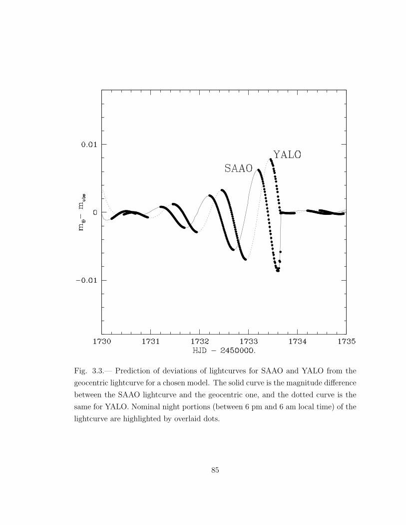
Fig. 3.3.— Prediction of deviations of lightcurves for SAAO and YALO from the

geocentric lightcurve for a chosen model. The solid curve is the magnitude difference

between the SAAO lightcurve and the geocentric one, and the dotted curve is the

same for YALO. Nominal night portions (between 6 pm and 6 am local time) of the

lightcurve are highlighted by overlaid dots.

85

Fig. 3.4.— Close-up of model lightcurves for the end of the second caustic crossing.

The solid curve is modeled for SAAO observations, the dotted curve is for YALO,

and the dashed curve is the geocentric lightcurve. The timing of the end of the

second crossing for SAAO is earlier than for YALO by 11 minutes. For comparison

purposes, all the lightcurve are calculated assuming no blend.

86

(Afonso et al. 2001). Comparison between their data and our model/observations

may serve as a confirmation of terrestrial parallax effects.

3.7. Measurement of the Projected Einstein Radius

Table 3.3 gives the parameters describing the best-fit microlens model (see

Appendix D for the discussion on the error determination) for the PLANET I-band

observations of EROS BLG-2000-5. We also transform the fit parameters to the

set of parameters introduced in § 3.6.1. In Table 3.4, we provide the result of

limb-darkening coefficient measurements. Because of the unprecedentedly long time

scale of the second caustic crossing and the extremely close approach to the cusp,

as well as the high quality of the data we adopt a two-parameter limb-darkening

law (eq. [2.5b]). The measurements of two coefficients, ΓI and ΛI are highly

anticorrelated so that the uncertainty along the major axis of error ellipse is more

than 50 times larger than that along its minor axis. While this implies that

the constraint on the surface brightness profile derived by the caustic crossing

lightcurve is essentially one dimensional, its natural basis is neither the linear nor

the square-root parameterized form. We plot, in Figure 3.5, the surface brightness

profile indicated by the fit and compare these with theoretical calculations taken

from Claret (2000). The figure shows that allowing the profile parameters to vary

by 2-σ does not have much effect on the central slope, but cause a large change in

87

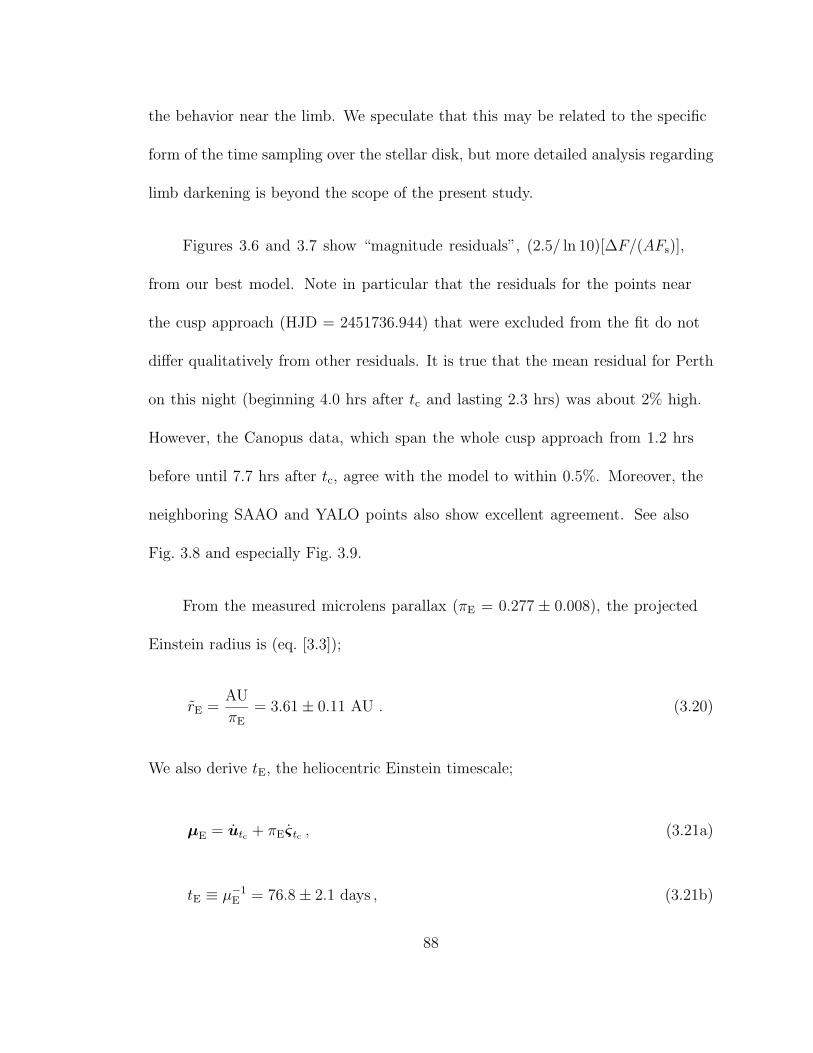
the behavior near the limb. We speculate that this may be related to the specific

form of the time sampling over the stellar disk, but more detailed analysis regarding

limb darkening is beyond the scope of the present study.

Figures 3.6 and 3.7 show “magnitude residuals”, (2.5/ ln 10)[∆F/(AFs)],

from our best model. Note in particular that the residuals for the points near

the cusp approach (HJD = 2451736.944) that were excluded from the fit do not

differ qualitatively from other residuals. It is true that the mean residual for Perth

on this night (beginning 4.0 hrs after tc and lasting 2.3 hrs) was about 2% high.

However, the Canopus data, which span the whole cusp approach from 1.2 hrs

before until 7.7 hrs after tc, agree with the model to within 0.5%. Moreover, the

neighboring SAAO and YALO points also show excellent agreement. See also

Fig. 3.8 and especially Fig. 3.9.

From the measured microlens parallax (πE = 0.277 ± 0.008), the projected

Einstein radius is (eq. [3.3]);

rE =AU

πE

= 3.61 ± 0.11 AU . (3.20)

We also derive tE, the heliocentric Einstein timescale;

µE = utc + πEς tc , (3.21a)

tE ≡ µ−1E = 76.8 ± 2.1 days , (3.21b)

88

Fig. 3.5.— Surface brightness profile of the source star. The thick solid curve is the

prediction indicated by the best fit model (see Table 3.4). In addition, the variation

of profiles with the parameters allowed to deviate by 2-σ along the direction of the

principal conjugate is indicated by a shaded region. For comparison, also shown

are theoretical profiles taken from Claret (2000). The stellar atmospheric model

parameters for them are log g = 1.0, [Fe/H]= −0.3, and Teff = 3500 K (dotted

curve), 4000 K (short dashed curve), 4500 K (long dashed curve). Note that the

effective temperature of the source is reported to be 4500 ± 250 K by Albrow et al.

(2001b).

89

Fig. 3.6.— “Magnitude” residuals from PLANET model of EROS BLG-2000-5.

Symbols are the same as in Fig. 3.1 The top panel shows the lightcurve corresponding

to the time of observations, the middle panel shows the averaged residuals from

15-sequential observations, and the bottom panel shows the scatters of individual

residual points.

90

Fig. 3.7.— Same as Fig. 3.6 but focuses mainly on the “anomalous” part of the

lightcurve. The middle panel now shows the daily averages of residuals.

91

and the direction of µE is 36.3 from ecliptic west to south. Since, toward the

direction of the event, the Galactic disk runs along 60.2 from ecliptic west to south,

µE points to 23.9 north of the Galactic plane. The overall geometry of the model is

shown in Figure 3.8, and Figure 3.9 shows a close-up of the geometry in the vicinity

of the cusp approach (t ∼ tc). Next, the projected velocity v on the observer plane

is

v = µErE = (−74.5 ± 3.1, 33.0 ± 11.0) km s−1 . (3.22)

Here the vector is expressed in Galactic coordinates. We note that the positive

x-direction is the direction of the Galactic rotation – i.e., the apparent motion of

the Galactic center seen from the Local Standard of Rest (LSR) is in the negative

x direction – while the positive y-direction is toward the north Galactic pole so

that the coordinate basis is lefthanded.

3.8. Measurement of the Angular Einstein Radius

The angular radius of the source, θ∗, is determined by placing the source on

an instrumental CMD and finding its offset relative to the center of the red giant

clump, whose dereddened and calibrated position toward the Galactic bulge are

known from the literature. For this purpose, we use the data obtained from YALO.

We find the instrumental I magnitude of the (deblended) source Is from the fit

92

Fig. 3.8.— Geometry of the event projected on the sky. Left is Galactic east, up is

Galactic north. The origin is the center of mass of the binary lens. The trajectory

of the source relative to the lens is shown as a thick solid curve while the short-

dashed line shows the relative proper motion of the source seen from the Sun. The

lengths of these trajectories correspond to the movement over six months between

HJD = 2451670 and HJD = 2451850. The circle drawn with long dashes indicates

the Einstein ring, and the curves within the circle are the caustics at two different

times. The solid curve is at t = tc while the dotted curve is at the time of the first

crossing. The corresponding locations of the two lens components are indicated by

filled (t = tc) and open (the first crossing) dots. The lower dots represent the more

massive component of the binary. The ecliptic coordinate basis is also overlayed

with the elliptical trajectory of πEς over the year.

93

Fig. 3.9.— Close-up of Fig. 3.8 around the cusp approach. The source at the closest

approach (t = tc) is shown as a circle. The solid curve is the caustic at t = tc while

the dotted curve is the caustic at the time of the first crossing. The positions of

the source center at the time of each of the observations are also shown by symbols

(same as in Figs. 3.1, 3.6, 3.7) that indicate the observatory. For the close-up panel,

only those points that were excluded from the fit because of numerical problems

in the magnification calculation (see §§ 3.5.1 and 3.7) are shown. Note that the

residuals for all points (included these excluded ones) are shown in Figs. 3.6 and

3.7.

94

to the lightcurve. To determine the color, we first note that, except when the

source is near (and so partially resolved by) a caustic, microlensing is achromatic.

That is, the source is equally magnified in V and I: FV = FV,b + AFV,s and

FI = FI,b + AFI,s. Hence, we assemble pairs of V and I points observed within 30

minutes (and excluding all caustic-crossing and cusp-approach data) and fit these

to the form FV = a1 + a2FI . We then find (V −I)s,inst = −2.5 log a2. We also find

the magnitude of the blend Ib from the overall fit, and solve for the color of the

blend (V −I)b,inst = −2.5 log[a2 + (a1/FI,b)].

We then locate the source on the instrumental CMD and measure its

offset from the center of the red giant clump; ∆(V −I) = 0.276 ± 0.010 and

∆I = 0.33 ± 0.02. Here, the quoted uncertainty includes terms for both the clump

center and the source position. Finally, using the calibrated and dereddened

position of the red clump, [(V −I)RC, IRC] = [1.114± 0.003, 14.37± 0.02] (Paczynski

et al. 1999), the source is at (V −I)s,0 = 1.390 ± 0.010, Is,0 = 14.70 ± 0.03.

The procedure does not assume any specific reddening law for determining the

dereddened source color and magnitude, but may be subject to a systematic error

due to differential reddening across the field.

We also perform a photometric calibration for observations made at SAAO.

The calibration was derived from images obtained on three different nights

by observing Landolt (1992) standards in the 2000 season, and the resulting

95

transformation equation were confirmed with a further night’s observations in

2001. Applying the photometric transformation on the fit result for the source flux,

we obtain the – unmagnified – source magnitude of Is = 16.602 in the standard

(Johnson/Cousins) system, while the standard source color is measured to be

(V −I)s = 2.69. By adopting the photometric offset between SAAO and YALO

instrumental system determined by the fit, we are able to derive a “calibrated”

YALO CMD for the field around EROS BLG-2000-5 (Fig. 3.10). The positions of

the source (S), blend (B), and clump center (C) are also overlaid on the CMD.

The CMD also implies that the reddening toward the field is AI = 1.90 and

E(V −I) = 1.30, which yields a reddening law, RVI = AV /E(V −I) = 2.46,

nominally consistent with the generally accepted RVI = 2.49 ± 0.02 (Stanek

1996). If we adopt a power-law extinction model Aλ ∝ λ−p, then RVI = 2.46

corresponds to p = 1.37. For this index, E(B−V )/E(V −I) = 0.838, which

predicts a lower extinction than the spectroscopically determined reddening of

E(B−V ) = 1.30 ± 0.05 by Albrow et al. (2001b).

Both the source and the blend lie redward of the main population of stars

in the CMD. One possible explanation is that the line of sight to the source is

more heavily reddened than average due to differential reddening across the field.

Inspection of the images does indicate significant differential reddening, although

from the CMD itself it is clear that only a small minority of stars in the field could

96

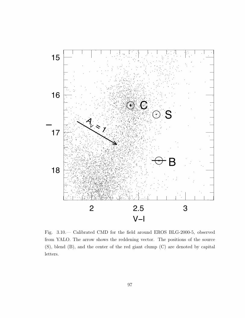
V−I

I

2 2.5 3

18

17

16

15

>

AV = 1

CS

B

Fig. 3.10.— Calibrated CMD for the field around EROS BLG-2000-5, observed

from YALO. The arrow shows the reddening vector. The positions of the source

(S), blend (B), and the center of the red giant clump (C) are denoted by capital

letters.

97

suffer the additional ∆AV ∼ 0.7 that would be necessary to bring the source to the

center of the clump. There is yet another indication that the source has average

extinction for the field – i.e., the same or similar extinction as the clump center.

The dereddened (intrinsic) color derived on this assumption, (V −I)s,0 = 1.39 is

typical of a K3III star (Bessell & Brett 1988), which is in good agreement with

the spectral type determined by Albrow et al. (2001b). On the other hand, if the

source were a reddened clump giant with (V −I)s,0 ∼ 1.11, then it should be a K1

or K2 star.

We then apply the procedure of Albrow et al. (2000a) to derive the angular

source radius θ∗ from its dereddened color and magnitude: first we use the

color-color relations of Bessell & Brett (1988) to convert from (V−I)s,0 to (V−K)s,0,

and then we use the empirical relation between color and surface brightness to

obtain θ∗ (van Belle 1999). From this, we find that

θ∗ = 6.62 ± 0.58 µas

= 1.42 ± 0.12 R kpc−1 , (3.23)

where the error is dominated by the 8.7% intrinsic scatter in the relation of van

Belle (1999). Alternatively, we use the different calibration derived for K giants

by Beuermann, Baraffe, & Hauschildt (1999) and obtain θ∗ = 6.47 µas, which is

consistent with equation (3.23). Finally, we note that if the source were actually

98

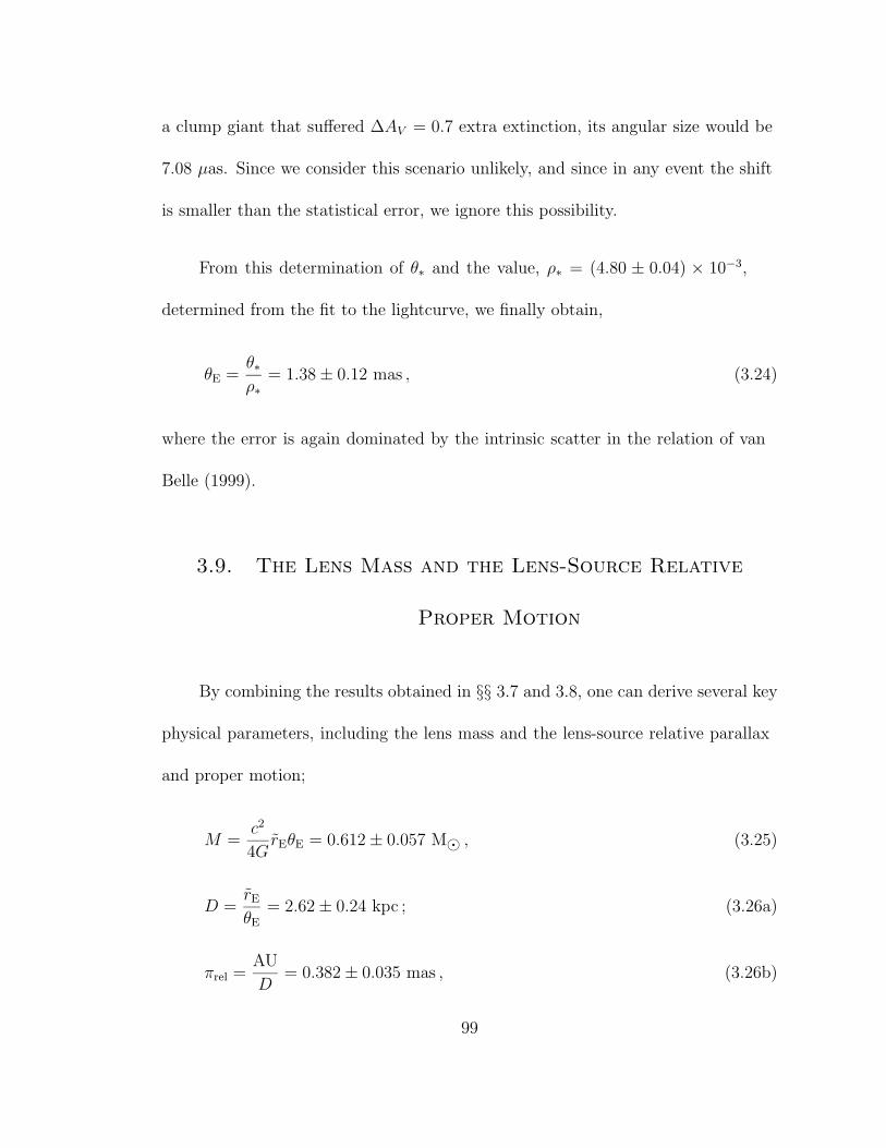
a clump giant that suffered ∆AV = 0.7 extra extinction, its angular size would be

7.08 µas. Since we consider this scenario unlikely, and since in any event the shift

is smaller than the statistical error, we ignore this possibility.

From this determination of θ∗ and the value, ρ∗ = (4.80 ± 0.04) × 10−3,

determined from the fit to the lightcurve, we finally obtain,

θE =θ∗ρ∗

= 1.38 ± 0.12 mas , (3.24)

where the error is again dominated by the intrinsic scatter in the relation of van

Belle (1999).

3.9. The Lens Mass and the Lens-Source Relative

Proper Motion

By combining the results obtained in §§ 3.7 and 3.8, one can derive several key

physical parameters, including the lens mass and the lens-source relative parallax

and proper motion;

M =c2

4GrEθE = 0.612 ± 0.057 M , (3.25)

D =rE

θE

= 2.62 ± 0.24 kpc ; (3.26a)

πrel =AU

D= 0.382 ± 0.035 mas , (3.26b)

99

µ = µEθE = 18.0 ± 1.7 µas day−1

= 31.1 ± 2.9 km s−1 kpc−1 . (3.27)

For the binary mass ratio of the best-fit model, q = 0.749, the masses

of the individual components are 0.350 M and 0.262 M, both of which

are consistent with the mass of typical mid-M dwarfs in the Galactic disk.

Using the mass-luminosity relation of Henry & McCarthy (1993), and adopting

MV = 2.89 + 3.37(V −I), the binary then has a combined color and magnitude

MI = 8.2 ± 0.2 and (V −I) = 2.54 ± 0.08. Since D−1 = D−1L − D−1

S , D is an upper

limit for DL, i.e., the lens is located in the Galactic disk within 2.6 kpc of the

Sun. Furthermore, an argument based on the kinematics (see § 3.10) suggests that

DS ∼> 8 kpc so that it is reasonable to conclude that DL ∼ 2 kpc (m−M 11.5).

Hence, even if the binary lens lay in front of all the extinction along the line of

sight, it would be ∼ 2 mag fainter than the blend (B), and so cannot contribute

significantly to the blended light. However, the proximity of the lens to the observer

is responsible for the event’s long time scale and quite large parallax effect.

100

3.10. The Kinematic Constraints on the Source

Distance

The projected velocity v (eq. [3.22]) is related to the kinematic parameters of

the event by

v = µD

=(D

vS

DS

− DvL

DL

+ v)⊥

, (3.28a)

where the final subscript, ⊥, serves to remind us that all velocities are projected

onto the plane of the sky. Writing v = vrot + v,p and vL = vrot + vL,p as the

sum of the Galactic rotation and the peculiar velocities and eliminating DL in favor

of D and DS, equation (3.28a) can be expressed as

v =[

D

DS

(vS − vrot) −(1 +

D

DS

)vL,p + v,p

]⊥

. (3.28b)

For a fixed DS and with a known Galactic kinematic model, the distribution

function of the expected value for v can be derived from equation (3.28b). The

measured value of v can therefore be translated into the relative likelihood, L for a

given DS and the assumed kinematic model,

− 2 lnL = (v − 〈v〉) · C−1 · (v − 〈v〉) + ln |C| + constant , (3.29a)

101

〈v〉 = xS(〈vS,⊥〉 − vrot) − (1 + xS)〈vL,p,⊥〉 + v,p,⊥ , (3.29b)

C = x2SC[vS,⊥] + (1 + xS)

2C[vL,⊥] + C[v] , (3.29c)

where C[vS,⊥] and C[vL,⊥] are the dispersion tensors for the source and the lens

transverse velocity, C[v] is the covariance tensor for the measurement of v, and

xS = D/DS.

We evaluate L as a function of DS assuming three different distributions

for vS,⊥ which respectively correspond to source being in the near disk

(〈vS,⊥〉 = vrot + 〈vS,p,⊥〉), bulge (〈vS,⊥〉 = 〈vS,p,⊥〉), and the far disk

(〈vS,⊥〉 = −vrot − 〈vS,p,⊥〉). Adopting the Galactic rotational velocity,

vrot = (220, 0) km s−1, the solar motion, v,p,⊥ = (5.2, 7.2) km s−1 (Binney &

Merrifield 1998), and the kinematic characteristics of the lens and the source given

in Table 3.5, we derive the relative likelihood as a function of source position

(Fig. 3.11), and find that the measured value of v (eq. [3.22]) mildly favors the far

disk over the bulge as the location of the source by a factor of ∼ 2.3. The near

disk location is quite strongly disfavored (by a factor of ∼ 10.6 compared to the far

disk, and by a factor of ∼ 4.7 compared to the bulge).

The complete representation of the likelihood for the source location requires

one to consider all the available constraints relevant to the source distance. In

particular, these include the radial (line-of-sight) velocity measurement and the

102

Fig. 3.11.— Kinematic likelihood for v as a function of DS. The three curves are for

different distributions of the source velocity: near-disk-like; vS = vrot + vS,p (short-

dashed line), bulge-like; vS = vS,p (solid line), and far-disk-like; vS = −vrot − vS,p

(long-dashed line). The top panel shows the likelihood derived using only the two-

dimensional projected velocity information while in the bottom panel, the likelihood

also includes the radial velocity information derived from the high resolution spectra

of Castro et al. (2001).

103

number density of stars constrained by the measured color and brightness (or

luminosity) along the line of sight. Although one may naively expect that a bulge

location is favored by the high density of stars in the bulge, which follows from

the fact that the line of sight passes within 400 pc of the Galactic center, it is not

immediately obvious how the disk contribution compares to the bulge stars for the

specific location of the source on the CMD (Fig. 3.10). Even with no significant

differential reddening over the field, the particular source position, which is both

fainter and redder than the center of the clump, can be occupied by relatively

metal-rich (compared to the bulge average) first ascent giants in either the bulge or

the far disk. Because first ascent giants become redder with increasing luminosity,

the source must have higher metallicity if it lies in the bulge than in the more

distant disk. ALthough there exists an estimate of the source metal abundance:

[Fe/H]= −0.3 ± 0.1 by Albrow et al. (2001b) based on VLT FORS1 spectra, to

incorporate these measurement into a likelihood estimate would require a more

through understanding of all the sources of error as well as a detailed model of

the metallicity distribution of the bulge and the disk. For this reason, we defer

the proper calculation of the likelihood in the absence of any definitive way to

incorporate the specific density function, and restrict ourselves to the kinematic

likelihood.

104

We determine the radial velocity of the source from Keck HIRES spectra of

Castro et al. (2001), kindly provided by R. M. Rich. We find the line-of-sight

velocity to be ∼ −100 km s−1 (blueshift; heliocentric), which translates to

∼ −90 km s−1 Galactocentric radial velocity accounting for the solar motion of

10 km s−1. The derived radial velocity strongly favors bulge membership of the

source since it is three times larger than the line-of-sight velocity dispersion for disk

K3 giants, but is consistent with the motions of typical bulge stars (c.f., Table 3.5).

Because the correlation between the radial and the transverse velocity for K3 giants

either in the disk or in the bulge is very small, the likelihood for the radial velocity

can be estimated independently from the likelihood for the transverse velocity, and

the final kinematic likelihood is a simple product of two components. We find that

the final kinematic likelihood including the radial velocity information indicates

that the source star belongs to the bulge (Fig. 3.11): the likelihood for the bulge

membership is about six times larger than that for the far disk membership.

Finally, we note that, if the source lay in the far disk, it should have an

additional retrograde proper motion of ∼ 4 mas yr−1 × (10 kpc/DS) with respect

to the bulge stars, which should be measurable using adaptive optics or the Hubble

Space Telescope.

105

3.11. Consistency between the Lens Mass and the

Binary Orbital Motion

For the derived parameters, we find a projected binary lens separation

r⊥ = dDLθE = 5.52 AU (5.25 AU) and transverse orbital speed

v⊥ = [d2 + (ωd)2]1/2DLθE = 2.76 km s−1 (2.62 km s−1) for DS = 10 kpc

(8 kpc). We can now define the transverse kinetic and potential energies

K⊥ = [q/(1 + q)2]Mv2⊥/2 and T⊥ = −[q/(1 + q)2]GM2/r⊥, and evaluate their ratio

(here and throughout this section, we assume that DS = 10 kpc),

⊥ ≡∣∣∣∣ T⊥K⊥

∣∣∣∣ =2GM

r⊥v2⊥

=c2

2

rEθE[r−1E + (DSθE)−1]3

d[d2 + (ωd)2]= 25.9 ± 5.1 . (3.30)

Here, the error is dominated by the uncertainty in the measurement of ω.

Since r⊥ ≤ r and v⊥ ≤ v, it follows that |T⊥| ≥ |T | and K⊥ ≤ K, and hence

|T⊥/K⊥| ≥ |T/K|, where |T/K| is the ratio of the true three-dimensional potential

and kinetic energies. The latter must be greater than unity for a gravitationally

bound binary. This constraint is certainly satisfied by EROS BLG-2000-5. Indeed,

perhaps it is satisfied too well. That is, what is the probability of detecting such a

large ratio of projected energies? To address this question, we numerically integrate

over binary orbital parameters (viewing angles, the orbital orientation and phase,

and the semimajor axis) subject to the constraint that r⊥ = 5.5 AU (DS = 10 kpc),

and at several fixed values of the eccentricity, e. We assume a random ensemble

106

of viewing angles and orbital phases. The results shown in Figure 3.12 assume a

Duquennoy & Mayor (1991) period distribution, but are almost exactly the same if

we adopt a flat period distribution. All of the eccentricities shown in Figure 3.12

are reasonably consistent with the observed ratio, although higher eccentricities are

favored.

One can also show that high eccentricities are favored using another

line of argument. First, note that |r⊥ × v⊥| = ωr2⊥ is the same as the

projection of the specific angular momentum of the binary to the line of sight,

|(r × v) · n| = 2πa2(1 − e2)| cos i|/P . Here a and P are the semimajor axis and

the orbital period of the binary, n is the line-of-sight unit vector, and i is the

inclination angle of the binary. Combining this result with Kepler’s Third Law,

4π2a3 = GMP 2, one obtains;

a(1 − e2)2 cos2 i =(ωr2

⊥)2

GM=

4

c2

ω2d4

rEθE[r−1E + (DSθE)−1]4

= 0.0013 ± 0.0341 AU . (3.31)

From the energy conservation, (v2/2) − (GM/r) = −GM/(2a), one may derive a

lower limit for a;

a =r

2

(1 − rv2

2GM

)−1

≥ r⊥2(1 − −1

⊥ )= 2.87 ± 0.09 AU . (3.32)

107

Fig. 3.12.— Distributions of the ratio of transverse potential energy, |T⊥| = [q/(1 +

q)2]GM2/r⊥ to transverse kinetic energy, K⊥ = [q/(1 + q)2]Mv2⊥/2, for binaries

seen at random times and random orientations, for three different eccentricities,

e = 0, 0.5, 0.9. Also shown is the 1 σ allowed range for EROS BLG-2000-5.

Noncircular orbits are favored.

108

The corresponding lower limit for the binary period is P ≥ 6.22 yr for DS = 10 kpc.

Now, we can derive a constraint on the allowed eccentricity and inclination by

dividing equation (3.31) by equation (3.32);

(1 − e2)| cos i| ≤ 0.021 ± 0.281 . (3.33)

The constraint here essentially arises from the fact that the fit barely detects

projected angular motion ω, while the formal precision of its measurement

corresponds to ∼ 80 yr orbital period in 1-σ level. For the observed projected

separation and the derived binary mass, this apparent lack of the binary angular

motion therefore naturally leads us to conclude that the binary orbit is either very

close to edge-on or highly eccentric (or both).

3.12. Another Look at MACHO 97-BLG-41

We have found that both parallax and binary orbital motion are required

to explain the deviations from rectilinear motion exhibited by the lightcurve of

EROS BLG-2000-5. In Albrow et al. (2000a), PLANET ascribed all deviations

from rectilinear motion for MACHO 97-BLG-41 to a single cause: projected binary

orbital motion. Could both effects have also been significant in that event as well?

Only detailed modeling can give a full answer to this question. However, we can

109

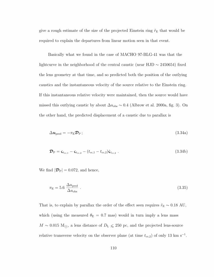
give a rough estimate of the size of the projected Einstein ring rE that would be

required to explain the departures from linear motion seen in that event.

Basically what we found in the case of MACHO 97-BLG-41 was that the

lightcurve in the neighborhood of the central caustic (near HJD ∼ 2450654) fixed

the lens geometry at that time, and so predicted both the position of the outlying

caustics and the instantaneous velocity of the source relative to the Einstein ring.

If this instantaneous relative velocity were maintained, then the source would have

missed this outlying caustic by about ∆uobs ∼ 0.4 (Albrow et al. 2000a, fig. 3). On

the other hand, the predicted displacement of a caustic due to parallax is

∆upred = −πEDP ; (3.34a)

DP = ς tcc,1 − ς tcc,2 − (tcc,1 − tcc,2)ς tcc,2 . (3.34b)

We find |DP| = 0.072, and hence,

πE = 5.6∆upred

∆uobs

. (3.35)

That is, to explain by parallax the order of the effect seen requires rE ∼ 0.18 AU,

which (using the measured θE = 0.7 mas) would in turn imply a lens mass

M ∼ 0.015 M, a lens distance of DL ∼< 250 pc, and the projected lens-source

relative transverse velocity on the observer plane (at time tcc,2) of only 13 km s−1.

110

While these values cannot be strictly ruled out, they are a priori extremely unlikely

because the optical depth to such nearby, low-mass, and slow lenses is extremely

small. On the other hand, if the lens lies at a distance typical of bulge lenses

DL ∼ 6 kpc and the source is a bulge star, then rE = DθE ∼ 17 AU, which would

imply ∆upred/∆uobs ∼ 1%. That is, parallax would contribute negligibly to the

observed effect. We therefore conclude that most likely parallax does not play a

major role in the interpretation of MACHO 99-BLG-47, but that detailed modeling

will be required to determine to what extent such a role is possible.

What is the physical reason that parallax must be so much stronger (i.e., πE

must be so much bigger) to have a significant effect in the case of MACHO 97-

BLG-41 than for EROS BLG-2000-5? Fundamentally, the former is a close binary,

and there is consequently a huge “lever arm” between the radial position of the

outlying caustic, uc ∼ 1.7 and the binary separation, d ∼ 0.5. That is uc/d ∼ 3.2.

This is almost an order of magnitude larger than for EROS BLG-2000-5, for which

uc ∼ 0.8 (Fig. 3.8), d ∼ 1.9, and uc/d ∼ 0.4. Consequently, parallax has to be

an order of magnitude larger to reproduce the effects of the same amount of the

projected binary orbital motion.

111

3.13. Summary

We have presented here results from two seasons of photometric I-band

monitoring of the microlensing event EROS BLG-2000-5, made by the PLANET

collaboration. The lightcurve exhibits two peaks which are well explained by a

finite source crossing over a fold-type – inverse-square-root singularity – caustic,

followed by a third peak which is due to the source’s passage close to a cusp.

We find no geometry involving a rectilinear source-lens relative trajectory and a

static lens that is consistent with the photometry. However, by incorporating both

parallax and binary orbital motion, we are able to model the observed lightcurve.

In particular, the detection of the parallax effect is important because it enables

us to derive the microlens mass, M = 0.612 ± 0.057 M, unambiguously by the

combination of the projected Einstein radius – measured from the parallax effect

– and the angular Einstein radius – inferred from the source angular size and

the finite source effect on the lightcurve. The source size is measurable from the

magnitude and the color of the source. The kinematic properties of the lens/source

system derived from our model together with the lens-source relative parallax

measurement as well as an additional radial velocity measurement indicate that the

event is most likely caused by a (K3) giant star in the bulge being lensed by a disk

binary (M dwarf) system about 2 kpc from the Sun. Additional information on

the specific density function along the line of sights, differential reddening across

112

the field, and a metallicity measurement of the source could further constrain the

source location.

113

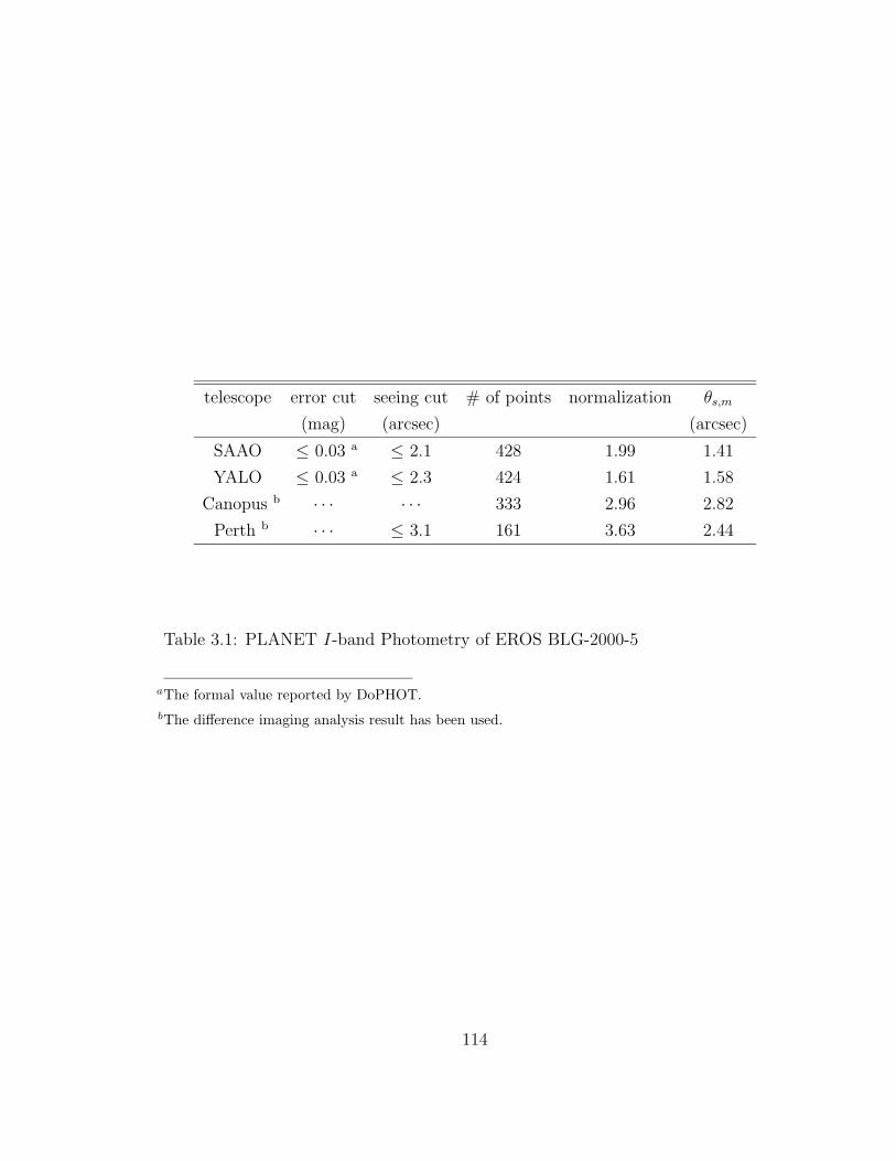
telescope error cut seeing cut # of points normalization θs,m

(mag) (arcsec) (arcsec)

SAAO ≤ 0.03 a ≤ 2.1 428 1.99 1.41

YALO ≤ 0.03 a ≤ 2.3 424 1.61 1.58

Canopus b · · · · · · 333 2.96 2.82

Perth b · · · ≤ 3.1 161 3.63 2.44

Table 3.1: PLANET I-band Photometry of EROS BLG-2000-5

aThe formal value reported by DoPHOT.bThe difference imaging analysis result has been used.

114

physical fit parameter

parameter

tc tc

q q

ρ∗ ρ∗πE (π2

E,‖ + π2E,⊥)1/2

dtc dtcπ−1E (πE,‖ew − πE,⊥en)

dtc π−1E [(dπE,‖ + ωdtcπE,⊥)ew + (−dπE,⊥ + ωdtcπE,⊥)en]

utc ucusp + ucπ−1E [(πE,⊥cosα′ − πE,‖sinα′)ew + (πE,‖cosα′ + πE,⊥sinα′)en]

utc t′−1E π−1

E [(πE,‖ cos α′ + πE,⊥ sin α′)ew − (πE,⊥ cos α′ − πE,‖ sin α′)en]

Table 3.2: Relations between Parameterizations. For simplicity, the reference times,

tc, for both systems are chosen to be the same: the time of the closest approach

to the cusp, i.e., (utc − ucusp) · utc = 0. The additional transformation of the

reference time requires the use of equations (3.17) and (3.19). Figure 3.2 illustrates

the geometry used for the derivation of the transformation. The unit vector en

points toward the NEP while ew is perpendicular to it and points to the west (the

direction of decreasing ecliptic longitude).

115

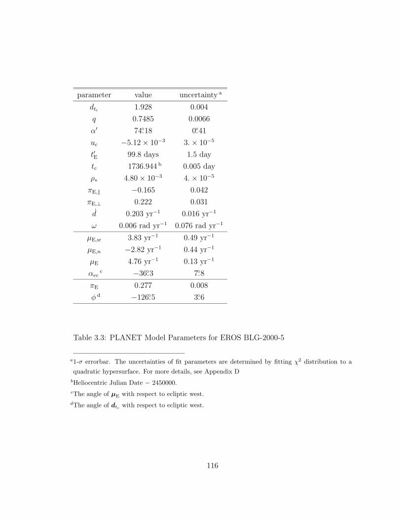
parameter value uncertainty a

dtc 1.928 0.004

q 0.7485 0.0066

α′ 74.18 0.41

uc −5.12 × 10−3 3. × 10−5

t′E 99.8 days 1.5 day

tc 1736.944 b 0.005 day

ρ∗ 4.80 × 10−3 4. × 10−5

πE,‖ −0.165 0.042

πE,⊥ 0.222 0.031

d 0.203 yr−1 0.016 yr−1

ω 0.006 rad yr−1 0.076 rad yr−1

µE,w 3.83 yr−1 0.49 yr−1

µE,n −2.82 yr−1 0.44 yr−1

µE 4.76 yr−1 0.13 yr−1

αecc −36.3 7.8

πE 0.277 0.008

φ d −126.5 3.6

Table 3.3: PLANET Model Parameters for EROS BLG-2000-5

a1-σ errorbar. The uncertainties of fit parameters are determined by fitting χ2 distribution to aquadratic hypersurface. For more details, see Appendix D

bHeliocentric Julian Date − 2450000.cThe angle of µE with respect to ecliptic west.dThe angle of dtc with respect to ecliptic west.

116

coefficient value

ΓI 0.452 ± 0.075

ΛI 0.011 ± 0.137

ΓI cos Φ + ΛI sin Φ a,b 0.207 ± 0.156

ΛI cos Φ − ΓI sin Φ c, b 0.402 ± 0.003

cI 0.552 ± 0.090

dI 0.011 ± 0.139

cI cos Ψ + dI sin Ψ a,d 0.290 ± 0.166

dI cos Ψ − cI sin Ψ c, d 0.470 ± 0.003

Table 3.4: Limb-Darkening Coefficients for EROS BLG-2000-5. The error bars

account only for the uncertainty in the photometric parameters restricted to a fixed

lens model, determined by the linear flux fit.

arotational transformation that maximizes the variancebΦ = −61.32crotational transformation that minimizes the variancedΨ = −57.14

117

location 〈vy〉 a σx σy σz

(km s−1) (km s−1) (km s−1) (km s−1)

vL,p disk −18 38 25 20

vS,p disk −11.5 31 21 17

bulge · · · 100 100 100

Table 3.5: Kinematic Characteristics of the Lens and the Source. The x-direction

is toward the Galactic center from the LSR, the y-direction is the direction of the

Galactic rotation, and the z-direction is toward the north Galactic pole. The lens

is assumed to be an M dwarf while the source is a K3 giant. The quoted values for

the disk components are derived from Binney & Merrifield (1998).

aasymmetric drift velocity

118

Chapter 4

Nonplanetary Microlensing Anomaly:

MACHO 99-BLG-47

4.1. Introduction

The hallmark of planetary microlensing events is a short deviation from an

otherwise normal, PSPL event. Mao & Paczynski (1991) showed that extrasolar

planets could be detected from such events, and Gould & Loeb (1992) gave an

explicit prescription for how the planet/star mass ratio q ( 1) and the angular

separation d (in units of the angular Einstein radius θE) could be reconstructed by

decomposing the event lightcurve into its “normal” and “perturbed” components.

Work during the ensuing decade has elucidated many additional subtleties of

planetary lightcurves, but their fundamental characterization as briefly perturbed

PSPL events has remained intact. Of particular importance in the present context,

119

Griest & Safizadeh (1998) showed that events with small impact parameter

(u0 1; where u0 is the minimum separation between the source and the lens

center of mass in units of θE) probe the so-called “central caustic” of the lens

geometry, making them much more sensitive to the presence of planets than the

larger impact-parameter events analyzed by Gould & Loeb (1992), which probe the

outer “planetary caustic”.

These central-caustic events are of exceptional importance, even though

they are intrinsically rare. They are rare simply because the central-caustic is

much smaller than the planetary caustic, so the great majority of planet-induced

deviations (of fixed fractional amplitude) are due to planetary caustics. However,

the probability of detecting a planet is much greater in small impact-parameter

events, partly because the source is guaranteed to pass close to the central caustic,

which almost by definition is near the center of the lens geometry (u = 0) and

partly because even the sensitivity of planetary caustics is enhanced for u0 1.

(Here u denotes the source position on the sky, normalized to θE, with respect to

the lens center of mass.) By contrast, higher impact-parameter events miss the

central caustic, and they are likely to miss the planetary caustic as well because

it lies in a random position relative to the source trajectory. Because of their

higher sensitivity to planets, and because they can be recognized in real time, low

impact-parameter events are monitored more intensively than typical events by

120

microlensing follow-up networks, which in turn further enhances their sensitivity to

planets.

Central-caustic events, like their planetary-caustic cousins, involve a short

deviation from an otherwise normal PSPL lightcurve. The major difference between

these two classes of planetary events is that central-caustic anomalies always occur

near the peak, whereas planetary-caustic perturbations can occur anywhere on the

lightcurve, and are typically expected on the wings of the lightcurve. Of particular

importance, for central-caustic events, there is no simple prescription for extracting

d and q by decomposing the lightcurve into “normal” and “perturbed” components

and it is unclear to what degree these two parameters are degenerate.

Another important, albeit accidental, discovery was that planets could give

rise to perturbations that are not short compared to the event timescale. In

the course of their search for planetary perturbations among 43 approximately

PSPL events, Gaudi et al. (2002, see also Albrow et al. 2001b) found one event,

OGLE-1999-BUL-36, that was asymmetric in a way that was consistent with

the presence of a planet. They argued, however, that the asymmetry was also

consistent with parallax effects induced by the Earth’s motion around the Sun of

the type analyzed by Gould et al. (1994), and that in general it would be extremely

difficult to distinguish between the two possible causes of such an asymmetry.

They concluded that, in most cases, microlensing searches are not able to

121

distinguish between parallax and a weak, asymmetric planetary perturbation, and

consequently, all such “detections” should be ignored. This reduces the sensitivity

of microlensing searches to planets, but only by an extremely small amount since,

as Gaudi et al. (2002) showed, long-timescale asymmetric perturbations account

for less than ∼ 1% of all planetary events. Hence, the long-timescale asymmetric

events also confirm in a way the basic paradigm: planetary perturbations have

short durations relative to the parent lightcurve, and in the rare cases for which

they do not, they are not recognizable as a planetary perturbation anyway.

However, not all short timescale deviations are due to planets and therefore the

mere detection of such an anomaly does not prove the presence of a planet. Gaudi

& Gould (1997) showed that close binaries (d 1) give rise to lightcurves that are

virtually identical to PSPL events, except when the source comes very close to the

lens center of mass (|u| 1). Hence, for events with u0 1, the lightcurve looks

“normal” except for a brief deviation near the peak. Qualitatively, this is exactly

the same behavior as that of central-caustic planetary events. Similarly, lightcurves

of wide-binary (d 1) events can also take the same form if one – and only one – of

the caustics lies very close to the source’s passage. Indeed, a close correspondence

between a certain pair of close-binary and wide-binary events was discovered both

theoretically (Dominik 1999) and observationally (Albrow et al. 1999c; Afonso et

al. 2000). It remains an open question under what conditions these various types

122

of events can be distinguished from one another. If central-caustic planetary events

could not be distinguished from close- and/or wide-binary events, it would seriously

undermine planet searches in high-magnification events and hence would call into

question the basic strategy adopted by microlensing follow-up groups (e.g., Albrow

et al. 1998).

Here we analyze the lightcurve of the microlensing event MACHO 99-BLG-47,

the first intensively monitored event with a short-lived, high S/N deviation from an

otherwise normal PSPL lightcurve. We identify the lens as an extreme-separation

binary rather than a planetary system, thereby showing that, at least in this case,

the two classes can be clearly distinguished. We also show that both wide- and

close-binary solutions fit the data equally well, implying that although planetary

perturbations can be distinguished from those arising from extreme-separation

binaries, the discrimination between very close and very wide binaries may be

difficult in practice.

4.2. MACHO 99-BLG-47

The initial alert for the microlensing event MACHO 99-BLG-47 was issued

by the MACHO collaboration on 1999 July 23.1 The event was located about

18 from the Galactic center along the disk (l = 1759′10′′, b = −157′36′′;

1 ftp://darkstar.astro.washington.edu/macho/Alert/99-BLG-47/

123

RA = 18h30m49.s4, Dec = −1410′53′′) and reported to be rather faint at baseline

(V = 21.5, R = 20.3). PLANET began monitoring MACHO 99-BLG-47 right after

the electronic alert with the expectation that it would be a very high magnification

event. PLANET detected anomalous behavior in the lightcurve during the first

week of August, and subsequently issued an anomaly alert on 1999 August 4.2

4.2.1. Observations and Data

The PLANET lightcurve of MACHO 99-BLG-47 consists of observations

made from three different southern sites: the Elizabeth 1 m at SAAO, Sutherland,

South Africa; the YALO 1 m at CTIO, La Serena, Chile; and the Canopus 1

m near Hobart, Tasmania, Australia. The observations were carried out in two

bands: I (at all three sites) and V (at SAAO only). The event was most intensely

monitored in 1999 August during and following the photometric peak and the

anomaly, but we obtained data through mid-September and also when the event

was close to baseline early in the 2000 season as the source came out from behind

the Sun. After the usual reductions, we perform photometry by two independent

methods: a direct fit to the PSF using DoPHOT (Schechter et al. 1993) and

difference imaging using ISIS (Alard & Lupton 1998; Alard 2000). For details,

see also Albrow et al. (2000a). Because of the different characteristics of the two

2 http://www.astro.rug.nl/˜planet/MB99047.html

124

methods and varying frame qualities, we recover a different number of photometric

measurements. Before any elaborate efforts to clean and select the data, we have

303 points from DoPHOT photometry and 297 from ISIS photometry (Table 4.1)

for the 1999 observations, as well as 8 points observed from YALO during early

2000 season (DoPHOT photometry only).

The photometric observations taken at SAAO are calibrated to the standard

Johnson-Cousins system with respect to E-region stars (Menzies et al. 1989)

observed contemporaneously with MACHO 99-BLG-47 at SAAO on 1999 July 31.

The instrumental magnitudes of observations from Canopus and YALO are not

calibrated explicitly, but rather we allow independent source fluxes for different

sites and bands in our modeling, which provide the relative photometric scalings

among them.

We also include in our analysis the publicly available MACHO photometry,

which comprises 77 VMACHO and 90 RMACHO points from the 1999 season as well

as 213 VMACHO and 227 RMACHO points taken between 1995 and 1998. The latter

were used to constrain the baseline and to check for source variability. We find no

evidence for such variability.

125

tele

scop

efilt

er#

ofto

talpoi

nts

#of

poi

nts

anal

yze

dm

edia

nse

eing

erro

rre

scal

ing

fact

or

(arc

sec)

PLA

NE

T(D

oPH

OT

)

Eliza

bet

h1

mI

9888

1.81

1.19

···

V26

241.

791.

02

Can

opus

1m

I51

422.

711.

43

YA

LO

1m

I12

812

21.

960.

772

PLA

NE

T(I

SIS

)

Eliza

bet

h1

mI

105

981.

651.

35

···

V21

201.

961.

83

Can

opus

1m

I57

382.

591.

75

YA

LO

1m

I11

411

01.

830.

919

MA

CH

O

Mt.

Str

omlo

50′′

RM

AC

HO

9090

···

1.04

···

VM

AC

HO

7776

···

0.70

9a /

0.73

0b

Tab

le4.

1:P

hot

omet

ric

dat

aof

MA

CH

O99

-BLG

-47.

aw

ith

resp

ect

toP

LA

NE

T/D

oPH

OT

mod

elbw

ith

resp

ect

toP

LA

NE

T/I

SIS

mod

el

126

The difference photometry is placed on an absolute scale by a linear regression

from the PSF-based flux (DoPHOT) to the differential flux (ISIS), after removing

obvious faulty points from the two data sets based on the reports by each

reduction/photometry package. We find that, except for the Canopus data, the

residuals of the PSF-based flux from the regression line are strongly correlated with

the size of the seeing disk, but that most of this correlation is removed by adding a

linear seeing correction. For example, for the SAAO I-band observations, we detect

the presence of a nonzero linear seeing dependence term of ∼ 1.7Fbase arcsec−1 (or

∼ 10Fs arcsec−1), with the S/N being as large as ∼ 30. Here Fs and Fbase are the

net flux of the lensed source star alone and the total flux in the same PSF when

there is no magnification.

In order to minimize the effects of known systematics, we optimize the data

set by rejecting outliers and reevaluating the sizes of the photometric error bars.

We also include a correction term for the correlation between the seeing and the

blended flux that enters the same PSF with the lensed source when we fit the

observed flux to a specific magnification model. These procedures are described in

detail and fully justified in the previous chapters as well as several earlier PLANET

papers (Albrow et al. 2000a,b, 2001b; Gaudi et al. 2002). Briefly, we first construct

an initial clean subset of the data by rejecting 3-σ outliers with respect to the linear

regression from DoPHOT to ISIS flux, and then determine a reference model based

127

on this subset. Once we have a reference model, we include all the data and follow

the same iterative procedure of outlier removal and error rescaling described in the

previous chapters. The final data set used for the subsequent analysis reported in

the present study contains 276 DoPHOT-reduced and 266 ISIS-reduced PLANET

points as well as 166 MACHO points (one VMACHO point rejected), all from the

1999 season (Table 4.1). The data obtained during seasons other than 1999 (the

2000 season YALO I, and the 1995 – 1998 season MACHO VMACHO and RMACHO

bands) are included in the analysis as a combined single point for each set. In

doing so, 4 data points (all RMACHO in the 1998 season) are eliminated as outliers.

4.3. Analysis and Model

The lightcurve of MACHO 99-BLG-47 (Fig. 4.1) is that of a normal

high-magnification PSPL event with a short-lived (∼ 3 days) deviation near the

peak, of the type predicted for planets (Griest & Safizadeh 1998) or binaries with

extreme separations. We therefore develop a method for probing the space of lens

geometries of this type and then search for the minimum χ2 within this space.

128

Fig. 4.1.— Observations and models of MACHO 99-BLG-47, all scaled to calibrated

Cousins I-band with blending as registered by SAAO DoPHOT photometry. Shown

are PLANET I-band from SAAO, Canopus, YALO, PLANET V -band from SAAO,

and MACHO VMACHO and RMACHO. The ISIS reduced PLANET points are plotted

after applying the transformation to the absolute scale derived from the linear

regression between difference photometry and PSF-based photometry. The solid

curve shows the final close-binary lens model fit (Table 4.2) to the data while the

dotted curve shows the “best” degenerate form of PSPL lightcurve (eq. [4.1]) fit

to a high-magnification subset of the data that excludes the anomalous points

near the peak. The half-magnitude offset between this curve and the data is

the main observational input into the algorithm to search for the final model (see

§ 4.3). Note that on the scale of the figure, the wide-binary solution is completely

indistinguishable from the close-binary solution, i.e., the solid curve can represent

both the close-binary and the wide-binary lens models equally well.

129

We begin by excising the anomalous points near the peak and fitting the

remaining lightcurve to the degenerate form of the Paczynski (1986) profile that

obtains in the high-magnification limit (Gould 1996),

F (t) =Fpeak√

1 + (t − t0)2/t2eff+ Fbase . (4.1)

Here F (t) is the instantaneous flux, Fpeak is the peak flux above the baseline of the

model, Fbase is the baseline flux, t0 is the time of the peak, and teff is the effective

width of the lightcurve. These degenerate parameters are related to the standard

parameters by Fpeak = Fs/u0, Fbase = Fs + Fb, and teff = u0tE, where tE is the

Einstein timescale. We find t0 ∼ 2451393.6 (Heliocentric Julian Date), teff ∼ 1 day,

and that Fpeak roughly corresponds to Ipeak ∼ 15.3 (Fig. [4.1]). However, the exact

values of those parameters are quite dependent on which points we excise. Note

that though the baseline magnitude is measured to be Ibase = 19.1, there is at this

point essentially no information of how the baseline flux divides into source flux

Fs and blended flux Fb, which is why it is necessary to fit the lightcurve to the

degenerate profile (eq. [4.1]).

Next, we reinsert the excised points near the peak and note that the maximum

(overmagnified) deviation from the degenerate fit is ∼ 0.5 mag (Fig. 4.1). We then

establish a set of initial trial event geometries as follows. For each diamond-shaped

caustic produced by various geometries of (d,q) pairs, we examine the magnification

130

as a function of distance from the “caustic center” along each of the three directions

defined by the four cusps of the caustic (one direction is redundant due to the

reflection symmetry with respect to the binary axis). Here for computational

simplicity, we use an analytic proxy point for the “caustic center,” defined as

follows. For close binaries, we adopt the center of mass of the lens system for the

caustic center. On the other hand, for wide binaries, the position of one component

of the binary shifted toward the other component by [d(1 + q−1)]−1 is chosen as the

caustic center. [These choices can be understood from the approximation developed

in 4.6. See also Dominik (1999).] Then, at each point u•, the point of the cusp-axis

crossing, we take the ratio of the actual magnification to that predicted for the

corresponding PSPL lens: a point mass lens located at the caustic center with the

same mass as either the whole binary (close binaries) or the nearest lens alone

(wide binaries). We proceed with the search only if this ratio lies in the interval

[1.2, 1.8]. We then choose a source trajectory perpendicular to the cusp axis as

an initial trial model, with u0 = |u•| and tE = teff/|u•|, and use four-parameter

(α, tE, t0, and u0) downhill simplex (Press et al. 1992) to search for a best-fit

model to minimize χ2, which is determined by a linear-flux fit to the model of lens

magnifications (and thus the corresponding Fs and Fb are found immediately),

subject to the constraint of fixed (d,q). Figure 4.2 shows the result of this search

(based on ISIS solutions) in a contour plot of χ2-surface over the (d,q)-space. The

χ2 is rising around all the boundaries shown in Figure 4.2, except toward lower

131

q. While the χ2-surface flattens with ∆χ2 32 as the mass ratio q becomes very

small (q ∼< 0.01) for d ∼ 0.065 and d ∼ 15, we find no evidence of a decrease of the

χ2 as q becomes smaller than 0.01. Rather it asymptotically approaches ∆χ2 32.

We find well-localized minima of χ2 over the searched (d,q)-space, one of

close binaries (d 0.13) and the other of wide binaries (d 11.3), whose exact

parameters depend slightly on whether we use the ISIS or DoPHOT photometry

(Tables 4.2 and 4.3). We adopt the ISIS solutions in the subsequent discussion (and

they are also what is shown in Fig. 4.2) because the lightcurve shows less scatter

and consequently, the errors for the model parameter determinations are smaller.

Despite the combination of the dense coverage near the peak by the PLANET

data and the extensive baseline coverage by the MACHO data, the final two ISIS

models (i.e., the close binary and the wide binary) are essentially indistinguishable:

∆χ2 = 0.6 for 412 degrees of freedom, with the close binary having the lower χ2 of

the two. In § 4.6, we discuss this degeneracy in further detail.

Finally, we also note that u0tE and Fs/u0 from the best-fit binary-lens model

parameters are not quite the same as the teff and Fpeak derived from the initial

degenerate form of the lightcurve fit. These discrepancies are traceable to small

differences between a true Paczynski (1986) curve and its degenerate approximation

(eq. [4.1]), and are not due to differences between the binary and corresponding

PSPL event, which are very small except around the peak. Since the parameters

132

Fig. 4.2.— Contour plot of χ2-surface over (d,q) space based on solutions for

PLANET (ISIS) and MACHO data. The binary separation d is in units of the

Einstein radius of the combined mass, and the mass ratio q is the ratio of the farther

component to the closer component to the source trajectory (i.e., q > 1 means that

the source passes by the secondary). Contours shown are of ∆χ2 = 1, 4, 9, 16, 25, 36

(with respect to the global minimum). We find two well-isolated minima of χ2, one

in the close-binary region, (d,q)=(0.134,0.340), and the other in the wide binary-

region, (d,q)=(11.31,0.751) with ∆χ2 = 0.6 and the close binary being the lower

χ2 solution. Also drawn are the curves of models with the same Q as the best-fit

close-binary model and the same γ as the best-fit wide-binary model (see 4.6).

133

parameters PLANET (ISIS) + MACHO PLANET (DoPHOT) + MACHO

d 0.134 ± 0.009 0.121 ± 0.009

q 0.340 ± 0.041 0.374 ± 0.058

tE 163 ± 26 days 183 ± 32 days

t0a, b 1393.9331 ± 0.0071 1393.9309 ± 0.0075

u0a (8.6 ± 1.1) × 10−3 (7.5 ± 1.3) × 10−3

α c 294.99 ± 0.25 294.45 ± 0.25

χ2 412.13 420.45

dof 412 423

Table 4.2: PLANET close-binary model of MACHO 99-BLG-47. We note that the

fact that χ2 ∼ dof results from our rescaling of the photometric errorbars. However,

we use the same scaling factor here and for models described in Table 4.3 so the

indistinguishableness between two models is not affected by this rescaling. The

uncertainties for parameters are “1-σ error bars” determined by a quadratic fit of

χ2 surface.

athe closest approach to the binary center of massbthe Heliocentric Julian Date − 2450000cthe binary center of mass lying on the righthand side of the moving source

134

parameters PLANET (ISIS) + MACHO PLANET (DoPHOT) + MACHO

d 11.31 ± 0.96 12.79 ± 1.05

q 0.751 ± 0.193 0.917 ± 0.288

tEa 220 ± 37 days 253 ± 47 days

t0b, c 1393.9113 ± 0.0072 1393.9133 ± 0.0074

u0a, b (6.5 ± 1.0) × 10−3 (5.50 ± 0.92) × 10−3

α d 295.46 ± 0.24 294.83 ± 0.24

χ2 412.74 420.50

dof 412 423

Table 4.3: PLANET wide-binary model of MACHO 99-BLG-47.

awith respect to the Einstein radius of the combined massbThe closest approach to the caustic center. See § 4.3 for the definition of the caustic center.cthe Heliocentric Julian Date − 2450000dthe caustic center lying on the righthand side of the moving source

135

derived from equation (4.1) function only as seeds for simplex, and since the final

χ2-surface is very well-behaved, these discrepancies in input values do not influence

the final result.

4.4. Discussion

The mass ratios of the best fit models are q = 0.340 ± 0.041 (close binary)

and q = 0.751 ± 0.193 (wide binary), which are well away from the regime of

planetary companions (q ∼< 0.01). By comparison, the ratio of the duration of the

anomalous portion of the lightcurve (tanom ∼ 3 days) to the Einstein timescale

(tE ∼ 160 days)3 is r = tanom/tE ∼ 0.02. For lightcurves perturbed by planetary

caustics, one typically finds q ∼ r2 (Gould & Loeb 1992). This relation clearly does

not apply to the caustics of extreme-separation binaries.

Models with q ≤ 0.01 (and q ≥ 100) are formally rejected at ∆χ2 32,

which is significant but not in itself an overwhelming rejection of the planetary

hypothesis. Hence, we examine the least χ2 model for q = 0.01 (∆χ2 = 32.3) for

its plausibility and the origin of statistical discriminating power. We discover that

the difference of χ2 is mostly from the MACHO data between HJD 2451310 and

3 While the value here is for the close binary, the value for the wide binary is essentially the

same because the relevant mass of the corresponding point-mass lens for the wide binary is not

the combined mass but the mass of the single component that the source passes by.

136

2451360, approximately 2 months prior to the photometric peak. However, we also

find that the “planetary” model exhibits an extremely high peak magnification

(Amax ∼ 15000), and consequently, requires the event to be much longer

(tE 40 yr) and more extremely blended (Is 25.7, Fs/Fbase 0.2%) than the

already unusually long and highly blended best-fit models. In addition, there is a

clear trend of increasing peak magnification (and thus timescale and blend as well)

as q is lowered beyond 0.01. This follows from the fact that the observed timescale

of the anomaly in the lightcurve essentially fixes the source movement relative

to the caustic. However, as q becomes smaller, the size of the caustic relative to

the Einstein ring shrinks, and therefore, the timescale of the event, that is the

time required for the source to cross the Einstein ring, increases. (Note that this

behavior causes a mild continuous degeneracy between q and the blending.) These

parameters determined for the “planetary” model are extremely contrived and

highly improbable a priori. Furthermore, the timescale associated with the “planet”

component, tp = q1/2tE ∼ 4 yr is much longer than that of typical stellar lenses,

which further reduces the plausibility of the planetary interpretation. In summary,

while in simple statistical terms, the star/planet scenario is not overwhelmingly

disfavored relative to extreme-separation binaries, we nevertheless can conclude

that it is highly unlikely that this event is due to a star/planet system.

137

From the standpoint of refining microlensing planet detection strategies, it

is important to ask how one could have discriminated between the planetary and

extreme-separation binary solutions with greater statistical significance. As noted

above, most of the discriminating power came from the MACHO data points on

the rising wing of the lightcurve, even though (or in a sense, because) these had

the largest errors and the lowest density of the nonbaseline coverage. That is,

the precision PLANET photometry over the peak and falling wing “predicts” the

rising wing for each of the models, but the noisier MACHO data can only roughly

discriminate between these predictions. Hence, the key would have been to get

better data on the rising part of the lightcurve. In practice this is difficult: the

MACHO data are noisier exactly because they are survey data, and one does not

know to monitor an event intensively until the lightcurve has actually started to

rise.

The long duration of the event, tE 160 days (close binary) or tE 220 days

(wide binary), may lead one to expect that the event would show some sign of

parallax effects (Gould 1992; Mao 1999; Soszynski, et al. 2001; Bennett et al.

2001). Similarly, the close passage of the source to a cusp could in principle give

rise to finite source effects (Gould 1994; Nemiroff & Wickramasinghe 1994; Witt

& Mao 1994), as for example is given in Chapter 2 for OGLE-1999-BUL-23 and

Chapter 3 for EROS BLG-2000-5. Indeed, in the case of EROS BLG-2000-5, the

138

combination of parallax and finite-source effects permitted us to measure the mass

of a microlens for the first time. We have therefore searched for both parallax and

finite source effects, but find no significant detection of either.

Finally, we examine the position of the source on the CMD (Fig. 4.3). The

most prominent feature found in the CMD is a track of stars running diagonally

in the same direction as would the main sequence. Since the field is in the

Galactic disk, this feature is probably not a true main sequence, but rather likely

to be a “reddening sequence”, that is, an ensemble of mostly disk turnoff stars

at progressively greater distances and correspondingly greater reddenings. The

baseline “star” (combined light of the source and blended light) lies within this

sequence toward its faint/red end although its position is seeing-dependent because

of the seeing-correction term. The position indicated in the CMD is plotted

assuming median seeing. However, the source itself [Is = 20.9, (V −I)s = 1.94] lies

∼ 2 mag below the baseline “star,” in a region of the CMD that is well below the

threshold of detection. If the baseline were mainly composed of source light, and

the “blended light” were simply source light that had been falsely attributed to

blending by a wrong model, then the real source would lie within the well populated

“reddening sequence”, and the timescale would be much shorter, tE ∼ 30 days. We

therefore searched for solutions with little or no blending. However, we find that

these are ruled out with ∆χ2 = 2440. Furthermore, the best-fit models with no

139

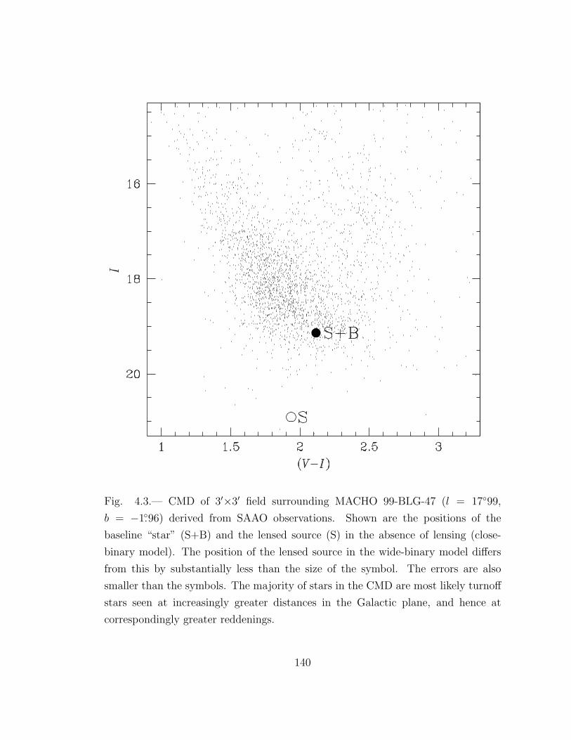
Fig. 4.3.— CMD of 3′×3′ field surrounding MACHO 99-BLG-47 (l = 1799,

b = −1.96) derived from SAAO observations. Shown are the positions of the

baseline “star” (S+B) and the lensed source (S) in the absence of lensing (close-

binary model). The position of the lensed source in the wide-binary model differs

from this by substantially less than the size of the symbol. The errors are also

smaller than the symbols. The majority of stars in the CMD are most likely turnoff

stars seen at increasingly greater distances in the Galactic plane, and hence at

correspondingly greater reddenings.

140

blended light are still extreme-separation binaries and not planetary systems. Since

we have only a crude understanding of the CMD, no strong argument can be made

that the position of the source is implausible. If, in fact, the observed track of

stars in Figure 4.3 is really the reddening sequence of disk turnoff stars, the source

position is consistent with a low-mass main sequence star lying ∼> 2 mag below the

turnoff. This would also explain the lack of finite source effect. Moreover, we note

that in disk fields, long events are not at all uncommon (Derue et al. 2001) because

the observer, source, and lens are all moving with roughly the same velocity.

Regarding the large amount of blended light required to fit the observed

lightcurve, we note that the highly significant seeing effect in the PSF-based

photometry (see § 4.2.1) is also evidence that the event is strongly blended.

In addition to the direct confirmation of the strong seeing effect from the

comparison between the differential flux and the PSF-based flux measurements,

we independently detect a significant seeing correction when we fit the observed

flux to the magnification model. For SAAO I-band observation, the seeing

correction determined from the model fit using DoPHOT flux is slightly smaller

(∼ 9Fs arcsec−1) than the value derived from the regression between DoPHOT

and ISIS flux. The seeing correction derived by fitting ISIS data to the model is

basically consistent with zero.

141

4.5. Binary Lens vs. Binary Source

Multiple-peak events like the one seen in Figure 4.1 can be caused by a binary

source (Griest & Hu 1992) rather than a binary lens. In general, one expects that

such events will be chromatic, since the colors of the two sources will not usually be

the same. By contrast, MACHO 99-BLG-47 is achromatic: the difference in color

of the two wings of the lightcurve is ∆V −I = 0.01 ± 0.05. In the limit that one

component of the binary is completely dark, the event will be achromatic, and yet

can have still have multiple peaks caused by orbital motion of the binary during

the event. In this case, however, there will be a series of roughly equally spaced

peaks that gradually die out as the event declines (Han & Gould 1997), contrary

to the distinct double-peaked behavior seen in Figure 4.1. Hence, a binary-source

explanation appears a priori implausible.

Nevertheless, it is possible in principle that the source has two components

of nearly identical color. We search for binary-source models, with either static

or slowly moving components, but find that the best fit model has ∆χ2 = 1167,

which clearly rules out such models. The basic problem is that the observed second

peak is very sharp given its height and the timescale of the declining lightcurve.

Binary-source lightcurves that fit these latter features tend to have a width that is

closer to that of the dotted curve in Figure 4.1. Recall that this curve represents a

single-lens degenerate fit to the nonpeak data. We conclude that the explanation

142

for the double-peaked behavior of the lightcurve is that it is a binary-lens rather

than a binary-source event.

4.6. Close and Wide Binary Correspondence

Dominik (1999) noticed that the Chang & Refsdal (1979, 1984) lens (CRL; see

also Schneider et al. 1992) well approximates the binary lens system in the vicinity

of each individual lens component of extreme wide-separation (d 1) binaries

and in the vicinity of the secondary of extreme close-separation (d 1) binaries

while the quadrupole lens (QL) approximation works nicely near the center of mass

of extreme close-separation binaries. He further showed that the size and shape

of the caustics and the behavior of the magnification field associated with them

are very similar among the true binary lenses, the CRL approximation, and the

QL approximation if the shear, γ, of the CRL and the absolute eigenvalue of the

quadrupole moment tensor, Q (for simplicity, hereafter Q will be just referred to

“the quadrupole moment”), of the QL are both very small and their numerical

values are close to each other (γ Q 1). These findings also imply the existence

of a correspondence between a wide binary with γ = d−2w qw(1 + qw)−1 and a close

binary with Q = d2cqc(1+ qc)

−2, sometimes referred to as a d ↔ d−1 correspondence.

(Here and throughout this section, we use the subscript c and w to distinguish the

143

parameters associated with the close and wide binaries.) Here we rederive the basic

result for this correspondence, and explore it more thoroughly.

The general form of the binary lens mapping equation can be expressed in

notation utilizing complex numbers (Witt 1990),

ζ = z − ε1

z − z1

− ε2

z − z2

, (4.2)

and the magnification associated with a single image can be found by,

A =

1 −

∣∣∣∣∣∂ζ

∂z

∣∣∣∣∣2

−1

, (4.3)

where ζ, z, z1, and z2 are the positions of the source, the image, and the two lens

components normalized by the Einstein radius of some mass, and ε1 and ε2 are the

masses of lens components in units of the same mass. For the extreme close-binary

case, if one chooses the center of mass as the origin and the binary axis as the

real axis and sets the combined mass to be unity, then z1 = dcε2, z2 = −dcε1,

ε1 = (1 + qc)−1, and ε2 = qc(1 + qc)

−1, and the lens equation (4.2) becomes

ζ = z − ε1

z − dcε2

− ε2

z + dcε1

(4.4)

≈ z − 1

z− d2

cε1ε2

z3+

d3cε1ε2(ε1 − ε2)

z4+ · · · (dc |z|) . (4.5)

Here the monopole term (z−1) is the same as for a PSPL and the first non-PSPL

term is the quadrupole (z−3), which acts as the main perturbation to the PSPL

144

if the quadrupole moment is small; Q = d2cε1ε2 = d2

cqc(1 + qc)−2 1. For a

given source position ζ, let the image position for the PSPL be z0. Then, under

the perturbational approach, the image for the QL approximation is found at

z = z0 + δzc, where |δzc| |z0| ∼ 1. Using the fact that z0 is the image position

corresponding to ζ for the PSPL (i.e., ζ = z0 − z−10 ), one obtains

δzc ≈ Q

(1 − 1

|z0|4)−1 [(

1

z30

− 1

z30 z

20

)+

(1

z40 z

20

− 1

z40

)1 − qc

1 + qc

dc + · · ·]

, (4.6)

from equation (4.5) and taking only terms linear in δzc and Q. Here, we note that

Q ∼ O(d2c) so that the second term in the bracket is lower order than Q2. In order

to find the magnification for this image, we differentiate equation (4.5), and find,

∂ζ

∂z≈ 1

z2+

3Q

z4

[1 − 4(1 − qc)

3(1 + qc)

dc

z+ · · ·

]. (4.7)

Then substituting z = z0 + δzc, for which δzc is given by equation (4.6), into

equation (4.7), we obtain,

∣∣∣∣∣∂ζ

∂z

∣∣∣∣∣2

≈ 1

|z0|4

+ Q

[3|z0|4 − 2|z0|2 − 1

|z0|8 − |z0|4(

1

z20

+1

z20

)

− 4|z0|4 − 2|z0|2 − 2

|z0|8 − |z0|4(

1

z30

+1

z30

)1 − qc

1 + qc

dc + · · ·]

. (4.8)

Note that the total magnification for the given source position is usually dominated

by one or two images found close to the critical curve. Thus, we consider only

145

the case for which the non-perturbed PSPL images lie close to the unit circle, so

we have |z0| = 1 + ∆ and ∆ 1. Then, we find the expression for the inverse

magnification for the QL approximation (up to the order of d3c),

A−1 ≈∣∣∣∣∣4∆ − 2Q

(1

z20

+1

z20

)+ 3Q

(1

z30

+1

z30

)1 − qc

1 + qc

dc

∣∣∣∣∣= 4

∣∣∣∣∣(|z0| − 1) − Q(z−20 ) +

3(1 − qc)

2(1 + qc)dcQ(z−3

0 )

∣∣∣∣∣ . (4.9)

For the extreme wide-binary case, one can rewrite the lens equation (4.2) as

ζ = z − 1

z− qw

z + d1

, (4.10)

≈ z − 1

z− qw

d1

+qw

d21

z − qw

d31

z2 + · · · (dw |z|) . (4.11)

Here the position and the mass of the first lens component are the origin and the

unit mass so that z1 = 0, z2 = −d1, ε1 = 1, ε2 = qw, and d1 = (1 + qw)1/2dw. We

note that, apart from the constant translation, the first non-PSPL term here is

essentially the shear, γ = qwd−21 = qwd−2

w (1 + qw)−1 for the CRL approximation.

Analogous to the extreme close binary, if γ 1, the image position for the

CRL approximation can be found by the perturbational approach, but here the

corresponding PSPL source position would be ζ + qwd−11 = z0 − z−1

0 . Then, the

image deviation δzw = z − z0 of CRL from PSPL is

δzw ≈ γ

(1 − 1

|z0|4)−1 [(

z0

z20

− z0

)+

(z20 −

z20

z20

)1

(1 + qw)1/2dw

+ · · ·]

. (4.12)

146

Using this result and the derivative of equation (4.11),

∂ζ

∂z≈ 1

z2+ γ

[1 − 2

(1 + qw)1/2

z

dw

+ · · ·]

, (4.13)

we find

∣∣∣∣∣∂ζ

∂z

∣∣∣∣∣2

≈ 1

|z0|4

+ γ

[ |z0|4 + 2|z0|2 − 3

|z0|4 − 1

(1

z20

+1

z20

)

− 2|z0|6 + 2|z0|4 − 4|z0|2|z0|4 − 1

(1

z30

+1

z30

)1

(1 + qw)1/2dw

+ · · ·]

. (4.14)

From the same argument used for the QL approximation of the extreme close

binary, we can set |z0| = 1 + ∆, and then the inverse magnification for the CRL

approximation (up to the order of d−3w ) is

A−1 ≈∣∣∣∣∣4∆ − 2γ

(1

z20

+1

z20

)+ 3γ

(1

z30

+1

z30

)1

(1 + qw)1/2dw

∣∣∣∣∣= 4

∣∣∣∣∣(|z0| − 1) − γ(z−20 ) +

3

2(1 + qw)1/2

γ

dw

(z−30 )

∣∣∣∣∣ . (4.15)

By comparing equations (4.9) and (4.15), we therefore establish the magnification

correspondence (up to the order of d2c ∼ d−2

w ) between the close binary with

Q = d2cqc(1+ qc)

−2 and the wide binary with γ = d−2w qw(1+ qw)−1 when Q γ 1.

For the two PLANET ISIS models for MACHO 99-BLG-47, we obtain

Q = 3.40 × 10−3 for the close binary solution (dc, qc) = (0.134, 0.340) and

147

γ = 3.35 × 10−3 for the wide binary solution (dw, qw) = (11.31, 0.751). Hence, the

observed degeneracy between the two PLANET models (see § 4.3 and Tables 4.2

and 4.3) is the clearest example of this type of correspondence observed so far.

While Afonso et al. (2000) reported that two different binary lens models, one of

a close binary and the other of a wide binary, can fit the observed lightcurve of

the (caustic-crossing) binary lens event, MACHO 98-SMC-1, one can infer from

their figure 8, that the degeneracy between the two models exists only for the

specific lightcurves (which is essentially a particular one dimensional slice of the

magnification field over the source plane) but not for the magnification field in

the neighborhood of the caustic as a whole. This is obvious from the relative

rotation of the two caustics. In addition, the source magnitudes for the two models

of MACHO 98-SMC-1 differ by ∼ 0.18 mag. By contrast, the difference of the

predicted Is between the two models of MACHO 99-BLG-47 is only ∼ 0.02 mag. In

fact, we get Q = 6.5× 10−2 (the close binary) and γ = 1.8× 10−2 (the wide binary)

for the two models of MACHO 98-SMC-1, and thus, although the degeneracy

of the MACHO 98-SMC-1 lightcurve is somehow related to the correspondence

of d ↔ d−1, it cannot be completely explained simply by the argument in this

section, and it should be investigated further for its origin. On the other hand,

the degeneracy of MACHO 99-BLG-47 is the first definitive observational case of

the correspondence between extreme separation binaries. This can be also seen in

148

Figure 4.4, which illustrates the similarity between the magnification fields for the

two models of MACHO 99-BLG-47.

The very low ∆χ2 between the two solutions despite the excellent data implies

that it is extraordinarily difficult to break this degeneracy with photometric data.

Gould & Han (2000) showed that for MACHO 98-SMC-1 the two solutions were

also astrometrically degenerate, at least for data streams lying within a few tE of

the peak. They argued that this astrometric degeneracy, like the corresponding

photometric degeneracy, was rooted in the lens equation. However, as shown

in this section, the correspondence between the equations describing close- and

wide-binaries is purely local (See also Dominik 2001). For example, there is a

constant-offset term in equation (4.11), which does not give rise to any local

photometric or astrometric effects, but which must “disappear” at late times. Hence

there must be a latetime astrometric shift between the two solutions. Such a shift

was noted explicitly by Gould & Han (2000) for the case of MACHO 98-SMC-1,

and these are likely to be a generic feature of close/wide corresponding pairs of

solutions.

We also plot the lines of (d,q) pairs that have the same shear γ as the

best-fit wide-binary model or the same quadrupole moment Q as the best-fit

close-binary model on χ2-surface contour plot shown in Figure 4.2. While

the iso-shear line for wide binaries lies nearly parallel to the direction of the

149

Fig. 4.4.— Grayscale plot of the difference of the normalized flux fields, 2|Fw −Fc|/(Fs,wAw + Fs,cAc) of the two PLANET models around the caustic. The two

fields are scaled and aligned so that the source trajectories coincide with each other.

The resulting shape and the relative size of the caustics are remarkably close to each

other [c.f., fig. 8 of Afonso et al. (2000) and Fig 2.6] Also drawn are the contours of

zero difference (dotted line) and 5% difference (solid line). While the actual source

trajectory (y = 0) naturally traces well the zero-difference line, the flux difference

would also be extremely small for other trajectories through the region, except very

near the caustic.

150

principal conjugate near the best-fit model, it is clear from the figure that the

condition of Q γ 1 alone does not define the observed well-defined twofold

degeneracy, which involves the additional correspondence between higher order

terms beyond the quadrupole moment (∼ d2c) and the pure shear (∼ d−2

w ).

Further comparison between equations (4.9) and (4.15) indicates that there exists

a magnification correspondence up to the order of d3c ∼ d−3

w if the condition

dc(1− qc)(1+ qc)−1 = d−1

w (1+ qw)−1/2 is also satisfied in addition to Q = γ 1. We

find that, for the two PLANET models, dc(1− qc)(1 + qc)−1 = 6.6× 10−2 (the close

binary) and d−1w (1 + qw)−1/2 = 6.7 × 10−2 (the wide binary). Hence, we conclude

that, in fact, these two conditions,

d2cd

2w(1 + qw) =

qw

qc

(1 + qc)2 , (4.16)

dcdw(1 + qw)1/2 =1 + qc

1 − qc

, (4.17)

define a unique correspondence between two extreme separation binaries. We also

note that the images (not shown) of the iso-∆χ2 contours for the close binary

models of MACHO 99-BLG-47 under the mapping defined by the above two

relations follows extremely closely the corresponding iso-∆χ2 contour for wide

binary models, except for the difference of ∆χ2 0.6 offset between two solutions.

151

4.7. Summary

MACHO 99-BLG-47 is the first microlensing event with a short-lived, high

S/N anomaly, characteristics that could betray the existence of a planet around

the lensing star. Nevertheless, we conclude that the lens of MACHO 99-BLG-47 is

not a planetary system, but an extreme-separation (very close or very wide) binary

composed of components of similar mass, based on the result of the lightcurve fit

as well as the extreme value of event duration and blending fraction required for

any plausible “planetary” fit.

152

BIBLIOGRAPHY

Afonso, C., et al. 2000, ApJ, 532, 340

Afonso, C., et al. 2001, A&A, 378, 1014

Alard, C., 2000, A&AS, 144, 363

Alard, C., & Lupton, R. H. 1998, ApJ, 503, 325

Albrow, M. D., et al. 1998, ApJ, 509, 687

Albrow, M. D., et al. 1999a, ApJ, 512, 672

Albrow, M. D., et al. 1999b, ApJ, 522, 1011

Albrow, M. D., et al. 1999c, ApJ, 522, 1022

Albrow, M. D., et al. 2000a, ApJ, 534, 894

Albrow, M. D., et al. 2000b, ApJ, 535, 176

Albrow, M. D., et al. 2001b, ApJ, 550, L173

Albrow, M. D., et al. 2001b, ApJ, 556, L113

Alcock, C., et al. 1995, ApJ, 454, L125

Alcock, C., et al. 1997, ApJ, 491, 436

Alcock, C., et al. 2000, ApJ, 541, 270

Bennett, D. P., et al. 1999, Nature, 402, 57

Bennett, D. P., et al. 2001, ApJ, submitted (astro-ph/0109467)

153

Bessell, M. S., & Brett, J. M. 1988, PASP, 100, 1134

Bessell, M. S., Castelli, F., & Plez, B. 1998, A&A, 333, 231

Beuermann, K., Baraffe, I., & Hauschildt, P. 1999, A&A, 348, 528

Binney, J., & Merrifield, M. 1998, Galactic Astronomy (Princeton, NJ: Princeton

University Press)

Boden, A. F., Shao, M., & van Buren, D. 1998, ApJ, 502, 538

Bogdanov, M. B., & Cherepashchuk, A. M. 1996, Astron. Rep., 40, 713

Bond, I. A., et al. 2001, MNRAS, 327, 868

Burns, D. et al. 1997, MNRAS, 209, L11

Castro, S. M., Pogge, R. W., Rich, R. M., DePoy, D. L., & Gould, A. 2001, ApJ,

548, L197

Chang, K., & Refsdal, S. 1979, Nature, 282, 561

Chang, K., & Refsdal, S. 1984, A&A, 132, 168

Claret, A. 1998a, A&AS, 131, 395

Claret, A. 1998b, A&A, 335, 647

Claret, A. 2000, A&A, 363, 1081

Claret, A., Dıaz-Cordoves, J., & Gimenez, A. 1995, A&AS, 114, 247

Derue, F., et al. 2001, A&A, 373, 126

Dıaz-Cordoves, J. & Gimenez, A. 1992, A&A, 259, 227

Dıaz-Cordoves, J., Claret, A., & Gimenez, A. 1995, A&AS, 110, 329

Dominik, M. 1999, A&A, 349, 108

Dominik, M. 2001, in ASP Conf. Ser. 237, Gravitational Lensing: Recent Progress

and Future Goals, ed. T. G. Brainerd & C. S. Kochanek (San Francisco, CA:

Astronomical Society of the Pacific)

Duquennoy, A., & Mayor, M. 1991, A&A, 248, 485

154

Gaudi, B. S., et al. 2002, ApJ, 566, 463

Gaudi, B. S., & Gould, A. 1997, ApJ, 482, 83

Gaudi, B. S., & Gould, A. 1999, ApJ, 513, 619

Gilliland, R. L., & Dupree, A. K. 1996, ApJ, 463, L29

Gould, A. 1992, ApJ, 392, 442

Gould, A. 1994, ApJ, 421, L71

Gould, A. 1995, ApJ, 441, L21

Gould, A. 1996, ApJ, 470, 201

Gould, A., & Andronov, N. 1999, ApJ, 516, 236

Gould, A., & Gaucherel, C. 1997, ApJ, 477, 580

Gould, A., & Han, C. 2000, ApJ, 538, 653

Gould, A., & Loeb, A. 1992, ApJ, 396, 104

Gould, A., Miralda-Escude, J., & Bahcall, J. N. 1994, ApJ, 423, L105

Gould, A., & Welch, D. L. 1996, ApJ, 464, 212

Grieger, B., Kayser, R., & Refsdal, S. 1986, Nature, 324, 126

Griest, K., & Hu, W. 1992, ApJ, 397, 362

Griest, K., & Safizadeh, N. 1998, ApJ, 500, 37

Hajian, A. R., et al. 1998, ApJ, 496, 484

Han, C., & Gould, A. 1997, ApJ, 480,196

Hardy, S. J., & Walker, M. A. 1995, MNRAS, 276, L79

Henry, T. J., & McCarthy, D. W. 1993, AJ, 106, 773

Hofmann, K.-H., & Scholz, M. 1998, A&A, 335, 637

Høg, E., Novikov, I. D., & Polanarev, A. G. 1995, A&A, 294, 287

155

Holz, D. E., & Wald, R. M. 1996, ApJ, 471, 64

Honma, M. 1999, ApJ, 517, L35

Kluckers, V. A., Edmunds, M. G., Morris, R. H., & Wooder, N. 1997, MNRAS,

284, 711

Landolt, A. U. 1992, AJ, 104, 340

Larsen, D. G., & Holdaway, R. 1999, The Astronomical Almanac for the Year 2000

(Washington, DC: US Government Printing Office)

Mao, S. 1999, A&A, 350, L19

Mao, S., et al. 2002, MNRAS, 329, 349

Mao, S., & Paczynski, B. 1991, ApJ, 374, L37

Menzies, J. W., Cousins, A. W. J., Banfield, R. M., & Laing, J. D. 1989, SAAO

Circ., 13, 1

Miyamoto, M., & Yoshii, Y. 1995, AJ, 110, 1427

Nemiroff, R. J., & Wickramasinghe, W. A. D. T. 1994, ApJ, 424, L21

Paczynski, B. 1986, ApJ, 304, 1

Paczynski, B. 1998, ApJ, 494, L23

Paczynski, B., Udalski, A., Szymanski, M., Kubiak, M., Pietrzynski, I., Wozniak,

P., & Zebrun, K. 1999, Acta Astron., 49, 319

Popper, D. M. 1984, AJ, 89, 132

Press, W. H., Teukolsky, S. A., Vetterling, W. T., & Flannery, B. P. 1982,

Numerical Recipes (Cambridge: Cambridge University Press)

Quirrenbach, A., Mozurkewich, D., Buscher, D. F., Hummel, C. A., & Armstrong,

J. T. 1996, A&A, 312, 160

Refsdal, S. 1966, MNRAS, 134, 315

Sasselov, D. D. 1997, in IAP Colloq. Proc. 12, Variable Stars and the Astrophysical

Returns of Microlensing Surveys, ed. R. Ferlet, J.-P. Maillard, & B. Raban (Gif

sur Yvette: Editions Frontieres), 141

156

Schechter, P. L., Mateo, M., & Saha, A. 1993, PASP, 105, 1342

Schneider, P., Ehlers, J., & Falco, E. E. 1992, Gravitational Lenses (Berlin:

Springer-Verlag)

Smith, M. C., Mao, S., & Wozniak 2001, MNRAS, submitted (astro-ph/0108214)

Soszynski, I., et al. 2001, ApJ, 552, 731

Stanek, K. Z. 1996, ApJ, 460, L37

Twigg, L.W. & Rafert, J.B. 1980, MNRAS, 193, 773

Udalski, A., Kubiak, M. & Szymanski, M. 1997, Acta Astron., 47, 319

Udalski, A., Szymanski, M., Kaluzny, J., Kubiak, M., & Mateo M. 1992, Acta

Astron., 42, 253

Valls-Gabaud, D. 1998, MNRAS, 294, 747

van Belle, G. T. 1999, PASP, 111, 1515

van Hamme, W. 1993, AJ, 106, 2096

Wade, R. A., & Rucinski, S. M. 1985, A&AS, 60, 471

Walker, M. A. 1995, ApJ, 453, 37

Wilson, R. E., & Devinney, E. J. 1971, ApJ, 166, 605

Witt, H. J. 1990, A&A, 236, 311

Witt, H. J. 1995, ApJ, 449, 42

Witt, H. J., & Mao, S. 1994, ApJ, 430, 505

157

Appendix A

Fold-Caustic Magnification of

Limb-Darkened Disk

If the point-source magnification due to a linear caustic is

Ar =(

ur

δu⊥

) 12

Θ(δu⊥) , (A.1a)

δu⊥ =θx − θc

θE

, (A.1b)

where the coordinate system is chosen so that the caustic lies parallel to y-direction

with x-coordinate of θc and the x-coordinate of the point source is θx, then the

magnification of the finite source with limb darkening at the origin is

A = F−1s,λ

∫∫Dd2θ ArSλ

=∫ ∞

−∞dθx Ar

∫dθy

Sλ(θx, θy)

Fs,λ

158

=∫ ∞

−∞dθx Ar

∫dθy

∫dθ′x δ(θ′x − θx)

Sλ(θ′x, θy)

Fs,λ

=∫ ∞

−∞dθx Ar

∫∫Dd2θ

Sλ(θ)

Fs,λ

δ(θ cos φθ − θx)

=∫ ∞

−∞dθx Ar

∫ θ∗

0θdθ

Sλ(θ)

Fs,λ

∫ π

−πdφθ δ(θ cos φθ − θx)

=∫ ∞

−∞dθx Ar

∫ θ∗

0θdθ

Sλ(θ)

Fs,λ

(θ2 − θ2x)

− 12 Θ(θ − |θx|)

=2(urθE)

12

πθ2∗

∫ ∞

−∞dθx (θx − θc)

− 12 Θ(θx − θc) Θ(θ∗ − |θx|)

×∫ θ∗

|θx|θdθ (θ2 − θ2

x)− 1

2

1 − ∑

m

Γm,λ

1 − m + 2

2

(1 − θ2

θ2∗

)m2

=2

π

(ur

θ∗/θE

) 12

Θ(θ∗ − θc)∫ θ∗

max(−θ∗,θc)

dθx

θ∗

(θx − θc

θ∗

)− 12

×∫ θ∗

|θx|θdθ

θ2∗

(θ2

θ2∗− θ2

x

θ2∗

)− 12

1 − ∑

m

Γm,λ

1 − m + 2

2

(1 − θ2

θ2∗

)m2

.(A.2a)

Here, δ(x) is Dirac delta distribution, Θ(x) is Heaviside step function, and Sλ(θ)

is the axis-symmetric surface brightness profile taken the form of equation (2.3).

Then, defining

Gn(η) ≡ 2(n + 1)

πΘ(1 − η)

∫ 1

max(−1,η)

dx

(x − η)12

∫ 1

|x|(1 − ρ2)nρ

(ρ2 − x2)12

dρ , (A.2b)

one obtains

A =

(ur

ρ∗

) 12

G0

(−∆u⊥

ρ∗

)+

∑m

Γm,λ

[Gm

2

(−∆u⊥

ρ∗

)− G0

(−∆u⊥

ρ∗

)]. (A.2c)

Here ∆u⊥ = −θc/θE is the distance to the caustic from the source center in units of

the Einstein ring radius and ρ∗ = θ∗/θE. Note that ∆u⊥ is positive when the source

159

center lies inside the caustic and vice versa. The second integral in equation (A.2b)

can be evaluated by using a new variable ν,

ν = arcsin

√ρ2 − x2

1 − x2; ρ2 = sin2 ν + x2 cos2 ν , (A.3a)

∫ 1

|x|(1 − ρ2)nρ

(ρ2 − x2)12

dρ = (1 − x2)n+ 12

∫ π/2

0dν (cos ν)2n+1

=

√π

2

n!

(n + 1/2)!(1 − x2)n+ 1

2 , (A.3b)

and therefore,

Gn(η) =1√π

(n + 1)!

(n + 1/2)!Θ(1 − η)

∫ 1

max(η,−1)dx

(1 − x2)n+ 12

(x − η)12

. (A.3c)

160

Appendix B

Determination of ς

If s is the Sun’s position vector with respect to the Earth normalized by 1 AU,

then the projection of s onto the plane of the sky, ς, is

ς = s − (s · n)n , (B.1)

where n is the line-of-sight unit vector toward the position of the event on the sky,

while the projection of p, the unit vector toward the north ecliptic pole (NEP), is

given by p = p − (p · n)n. Then, (ςw, ςn), the ecliptic coordinate components of ς,

are

ςw =(p × ς) · n

|p| =(p × s) · n√1 − (p · n)2

, (B.2a)

ςn =p · ς|p| = − (p · n)(s · n)√

1 − (p · n)2, (B.2b)

161

where we make use of p · s = 0. One can choose three-dimensional coordinate axes

so that the x-axis is the direction of the vernal equinox, the z-axis is the direction

to the NEP, and y = z × x. Then,

p = (0, 0, 1) ; (B.3a)

s = (r⊕ cos λ, r⊕ sin λ, 0) ; (B.3b)

n = (cos λ0 cos β0, sin λ0 cos β0, sin β0) , (B.3c)

where r⊕ is the distance to the Sun from the Earth in units of AU, λ is the

Sun’s ecliptic longitude, and (λ0, β0) are the ecliptic coordinates of the event. By

substituting equations (B.3) into equations (B.2), one finds that

ςw = −r⊕ sin(λ − λ0) , (B.4a)

ςn = −r⊕ cos(λ − λ0) sin β0 . (B.4b)

In general, one must consider the Earth’s orbital eccentricity (ε = 1.67× 10−2)

to calculate ς for any given time. Then,

r⊕ = 1 − ε cos ψ ; λ = ξ − φΥ , (B.5a)

ψ − ε sin ψ = Ωt , (B.5b)

162

sin ξ =(1 − ε2)1/2 sin ψ

1 − ε cos ψ; cos ξ =

cos ψ − ε

1 − ε cos ψ, (B.5c)

where ψ and ξ are the eccentric and true anomalies of the Earth, φΥ = 77.86 is

the true anomaly at the vernal equinox (March 20, 07h35m UT for 2000; Larsen &

Holdaway 1999), t is the time elapsed since perihelion, and Ω = 2π yr−1. Note that

the Earth was at perihelion at January 3, 05h UT for 2000 (Larsen & Holdaway

1999). Although equations (B.5) cannot be solved for r⊕ and λ in closed form

as functions of t, one can expand in series with respect to ε and approximate up to

the first order (epicycle approximation) so that

r⊕ = 1 − ε cos(Ωt) ; λ = Ωt − φΥ + 2ε sin(Ωt) . (B.6)

163

Appendix C

Microlens Diurnal Parallax

The angular position of a celestial object observed from an observatory on the

surface of the Earth is related to its geocentric angular position, ϕX by

ϕ′X = ϕX − γR⊕

DX

, (C.1)

where

γ = r − (r · n)n (C.2)

is the projection of the position vector, r, of the observatory with respect to the

center of the Earth, onto the plane of the sky and normalized by the mean radius

of the Earth, R⊕; and DX and n are the distance and the line-of-sight vector to

the object of interest. If one observe a microlensing event, the actual dimensionless

164

lens-source separation vector therefore differs from u (eq. [3.17]) by

u′ =ϕ′

S − ϕ′L

θE

= u +R⊕rE

γ

= υ + (t − tc)µE − πE(ς − R⊕AU

γ) . (C.3)

To find the algebraic expression for ecliptic coordinate components of γ, we

choose the same coordinate axes as for equations (B.3). Then, the position vector,

r is expressed as

r = (cosδg cosτΥ, cosδg sinτΥ cosε + sinδg sinε, sinδg cosε − cosδg sinτΥ sinε) ,

(C.4)

where δg is the geographic latitude of the observatory, τΥ is the hour angle of the

vernal equinox (i.e. the angle of the local sidereal time) at the observation, and

ε = 23.44 is the angle between the direction toward the north celestial pole and the

NEP (here we also assume that the Earth is a perfect sphere). Then, following a

similar procedure as in B,

γw =(p × γ) · n

|p| =(p × r) · n√1 − (p · n)2

; (C.5a)

γn =p · γ|p| =

p · r − (p · n)(r · n)√1 − (p · n)2

, (C.5b)

165

one obtains the ecliptic coordinate components of γ,

γw = − sinδg sinε cosλ0 + cosδg(cosτΥ sinλ0 − sinτΥ cosε cosλ0) ; (C.6a)

γn = sinδg(cosε cosβ0 − sinε sinλ0 sinβ0)

− cosδg[cosτΥ cosλ0 sinβ0 + sinτΥ(sinε cosβ0 + cosε sinλ0 sinβ0)] . (C.6b)

166

Appendix D

Hybrid Statistical Errors

As we described in § 3.6.2, our χ2 minimization procedure is effective at

fixed (d, q) (with the nine other geometrical parameters allowed to vary), but does

not work when all 11 geometrical parameters are allowed to vary simultaneously.

We therefore find the global minimum by evaluating χ2 over a (d, q) grid. How

can the errors, and more generally the covariances, be determined under these

circumstances?

In what follows, the parameters will be collectively represented by a vector ai

and the indices i, j will be allowed to vary over all p = 11 parameters. We assign

a1 = d and a2 = q, and designate that the indices m,n will be restricted to these

two parameters. What we seek to evaluate is cij = cov(ai, aj) ≡ 〈aiaj〉 − 〈ai〉〈aj〉.

First we note that it is straightforward to determine cmn: simply

evaluate χ2 at a series of points on the (a1, a2) grid, and fit these to

167

χ2 = χ2min +

∑2m,n=1 bmn(am − amin

m )(an − aminn ). Then (cmn) = (bmn)−1 is

the covariance matrix restricted to the first two parameters, i.e., cmn = cmn.

Next, at fixed (a1, a2) = (a†1, a

†2), we evaluate the restricted covariance matrix

of the remaining p−2 = 9 parameters by varying 0, 1, or 2 parameters at a time and

fitting the resulting χ2 hypersurface to χ2 = χ2min +

∑11i,j=3 bij(ai − amin

i )(aj − aminj ).

Then, using equations (E.5), one can show that (cij) = (bij)−1 is related to the full

covariance matrix by

cij = cij −∑m,n

bmncmicnj (i, j = 1, 2) , (D.1)

and the parameters, ai, at the constrained minimum are

ai = amini − ∑

m,n

(aminm − a†

m)bmncni (i = 1, 2) . (D.2)

Differentiating equation (D.2) with respect to a†m yields

∂ai

∂a†m

=∑n

bmncni , (D.3)

cmi =∑n

cmn∂ai

∂a†n

. (D.4)

The partial derivatives can be determined simply by finding the change in ai as

one steps along one axis of the (d, q) grid. Since cmn is already known from the

168

first step, above, the cmi are also known. Finally, the remaining covariances can be

found by substituting equation (D.4) into equation (D.1),

cij = cij +∑m,n

cmn∂ai

∂a†m

∂aj

∂a†n

. (D.5)

169

Appendix E

Minimization with Constraints

We use Lagrange multipliers to evaluate the n-dimensional vector ai that

minimizes the quadratic function H(ai) =∑n

i,j=1 bij(ai−a0i )(aj−a0

j)+H0, subject

to the m linear constraints∑n

i=1 aiαki = zk (k = 1, . . . ,m). Here the a0

i , the bij, and

H0 are constants. At this minimum, ∇H must lie in the m-dimensional subspace

spanned by the constraint vectors αli, i.e.,

∑nj=1 bij(aj − a0

j) +∑m

l=1 αliD

l = 0, or

ai = a0i −

m∑l=1

Dlκli ; κl

i ≡n∑

j=1

cijαlj , (E.1)

where (cij) ≡ (bij)−1, and the Dl are constants to be determined. Multiplying

equation (E.1) by each of the αki yields a set of m equations,

m∑l=1

CklDl =n∑

i=1

a0i α

ki − zk ; Ckl ≡

n∑i=1

αki κ

li =

n∑i,j=1

cijαki α

lj , (E.2)

170

which can be inverted to solve for the Dk,

Dk =m∑

l=1

Bkl

(n∑

i=1

a0i α

li − zl

);

(Bkl

)=

(Ckl

)−1. (E.3)

Note that for the special case where H can be interpreted as χ2,

cij is the covariance matrix of the unconstrained parameters ai, i.e.,

cij = cov(ai, aj) = 〈aiaj〉 − 〈ai〉〈aj〉. One then finds by direct substitution

that cov(Dk, a0i ) =

∑ml=1 Bklκl

i, so that the covariances of the constrained

parameters cij = cov(ai, aj), are given by

cij = cij −m∑

k,l=1

Bklκki κ

lj . (E.4)

To further specialize to an important subcase, let αki = δik. Then κk

i = cik

and Ckl = ckl, hence Bkl = bkl, where (bkl) = (ckl)−1 and ckl is the (unconstrained)

m×m covariance matrix restricted to the m parameters that are to be constrained.

Thus, for this special case, equations (E.1), (E.3), and (E.4) become

ai = a0i −

m∑k,l=1

cikbkl(a0l − zl) ; cij = cij −

m∑k,l=1

bklcikcjl . (E.5)

171