Astrophysics
117
June 17, 2013 11:29 World Scientific Book - 9in x 6in book Publishers’ page i
-
Upload
jeffrey-rable -
Category
Documents
-
view
11 -
download
4
description
By Serguei Komissarov
Transcript of Astrophysics

June 17, 2013 11:29 World Scientific Book - 9in x 6in book
Publishers’ page
i

June 17, 2013 11:29 World Scientific Book - 9in x 6in book
Publishers’ page
ii

June 17, 2013 11:29 World Scientific Book - 9in x 6in book
Publishers’ page
iii

June 17, 2013 11:29 World Scientific Book - 9in x 6in book
Publishers’ page
iv

June 17, 2013 11:29 World Scientific Book - 9in x 6in book
Dedication Page
(optional)
v

June 17, 2013 11:29 World Scientific Book - 9in x 6in book
vi Magnetic fields in Relativistic Astrophysics

June 17, 2013 11:29 World Scientific Book - 9in x 6in book
Preface
There will be a preface.
Serguei Komissarov
vii

June 17, 2013 11:29 World Scientific Book - 9in x 6in book
viii Magnetic fields in Relativistic Astrophysics

June 17, 2013 11:29 World Scientific Book - 9in x 6in book
Contents
Preface vii
Metric space and Tensor Calculus 1
1. From Euclidean space to surfaces and metric manifolds 3
1.1 Metric form . . . . . . . . . . . . . . . . . . . . . . . . . 3
1.1.1 The notion of metric form . . . . . . . . . . . . . 3
1.1.2 Metric forms of surfaces: . . . . . . . . . . . . . . 5
1.1.3 Locally Cartesian coordinates: . . . . . . . . . . . 6
1.1.4 Lengths of curves . . . . . . . . . . . . . . . . . . 7
1.1.5 Coordinate transformations: . . . . . . . . . . . . 7
1.2 Vectors, bases, and components of vectors . . . . . . . . . 8
1.2.1 Coordinate bases . . . . . . . . . . . . . . . . . . 8
1.2.2 Coordinate transformations . . . . . . . . . . . . . 10
1.3 Metric form and the scalar product . . . . . . . . . . . . . 10
1.4 Geodesics and the variational principle . . . . . . . . . . . 12
1.4.1 Euler-Lagrange Theorem . . . . . . . . . . . . . . 12
1.4.2 Geodesics . . . . . . . . . . . . . . . . . . . . . . . 12
1.4.3 Examples of geodesics: . . . . . . . . . . . . . . . 14
1.5 Non-Euclidean geometry of a Euclidean sphere . . . . . . 15
1.6 Manifolds . . . . . . . . . . . . . . . . . . . . . . . . . . . 16
1.7 Vectors as operators . . . . . . . . . . . . . . . . . . . . . 17
1.7.1 Basic idea . . . . . . . . . . . . . . . . . . . . . . 17
1.7.2 Coordinate transformations . . . . . . . . . . . . . 18
1.7.3 Magnitudes of vectors and the scalar product . . . 19
ix
June 17, 2013 11:29 World Scientific Book - 9in x 6in book
x Magnetic fields in Relativistic Astrophysics
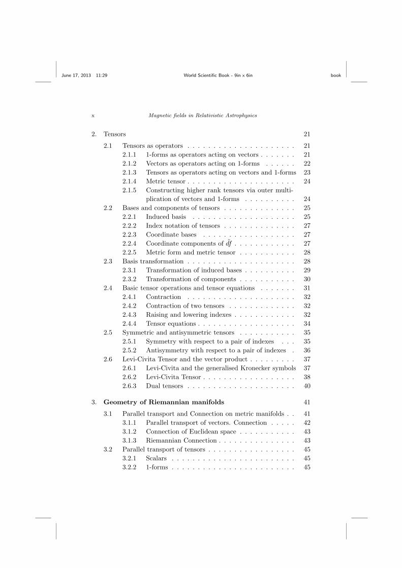
2. Tensors 21
2.1 Tensors as operators . . . . . . . . . . . . . . . . . . . . . 21
2.1.1 1-forms as operators acting on vectors . . . . . . . 21
2.1.2 Vectors as operators acting on 1-forms . . . . . . 22
2.1.3 Tensors as operators acting on vectors and 1-forms 23
2.1.4 Metric tensor . . . . . . . . . . . . . . . . . . . . . 24
2.1.5 Constructing higher rank tensors via outer multi-
plication of vectors and 1-forms . . . . . . . . . . 24
2.2 Bases and components of tensors . . . . . . . . . . . . . . 25
2.2.1 Induced basis . . . . . . . . . . . . . . . . . . . . 25
2.2.2 Index notation of tensors . . . . . . . . . . . . . . 27
2.2.3 Coordinate bases . . . . . . . . . . . . . . . . . . 27
2.2.4 Coordinate components of df . . . . . . . . . . . . 27
2.2.5 Metric form and metric tensor . . . . . . . . . . . 28
2.3 Basis transformation . . . . . . . . . . . . . . . . . . . . . 28
2.3.1 Transformation of induced bases . . . . . . . . . . 29
2.3.2 Transformation of components . . . . . . . . . . . 30
2.4 Basic tensor operations and tensor equations . . . . . . . 31
2.4.1 Contraction . . . . . . . . . . . . . . . . . . . . . 32
2.4.2 Contraction of two tensors . . . . . . . . . . . . . 32
2.4.3 Raising and lowering indexes . . . . . . . . . . . . 32
2.4.4 Tensor equations . . . . . . . . . . . . . . . . . . . 34
2.5 Symmetric and antisymmetric tensors . . . . . . . . . . . 35
2.5.1 Symmetry with respect to a pair of indexes . . . 35
2.5.2 Antisymmetry with respect to a pair of indexes . 36
2.6 Levi-Civita Tensor and the vector product . . . . . . . . . 37
2.6.1 Levi-Civita and the generalised Kronecker symbols 37
2.6.2 Levi-Civita Tensor . . . . . . . . . . . . . . . . . . 38
2.6.3 Dual tensors . . . . . . . . . . . . . . . . . . . . . 40
3. Geometry of Riemannian manifolds 41
3.1 Parallel transport and Connection on metric manifolds . . 41
3.1.1 Parallel transport of vectors. Connection . . . . . 42
3.1.2 Connection of Euclidean space . . . . . . . . . . . 43
3.1.3 Riemannian Connection . . . . . . . . . . . . . . . 43
3.2 Parallel transport of tensors . . . . . . . . . . . . . . . . . 45
3.2.1 Scalars . . . . . . . . . . . . . . . . . . . . . . . . 45
3.2.2 1-forms . . . . . . . . . . . . . . . . . . . . . . . . 45

June 17, 2013 11:29 World Scientific Book - 9in x 6in book
Contents xi
3.2.3 General tensors . . . . . . . . . . . . . . . . . . . 46
3.2.4 Metric tensor . . . . . . . . . . . . . . . . . . . . . 46
3.3 Absolute and covariant derivatives . . . . . . . . . . . . . 47
3.3.1 Absolute and covariant derivatives of scalar fields 48
3.3.2 Absolute and covariant derivatives of vector fields 48
3.3.3 Absolute and covariant derivatives of 1-form fields 49
3.3.4 Absolute and covariant derivatives of general ten-
sor fields . . . . . . . . . . . . . . . . . . . . . . . 50
3.3.5 General properties of covariant differentiation . . 51
3.3.6 The field of metric tensor . . . . . . . . . . . . . . 51
3.4 Divergence . . . . . . . . . . . . . . . . . . . . . . . . . . 52
3.5 Geodesics and parallel transport . . . . . . . . . . . . . . 54
3.6 Geodesic coordinates and Fermi coordinates . . . . . . . . 56
3.6.1 Geodesic coordinates . . . . . . . . . . . . . . . . 56
3.6.2 Fermi coordinates . . . . . . . . . . . . . . . . . . 58
3.7 Riemann curvature tensor . . . . . . . . . . . . . . . . . . 60
3.8 Properties of the Riemann curvature tensor . . . . . . . . 64
3.9 Ricci tensor, curvature scalar and the Einstein tensor . . . 65
Basic Theory of Relativity 67
4. Space and time in the theory of relativity 69
4.1 Space and Time in Newtonian Physics . . . . . . . . . . . 69
4.1.1 Time . . . . . . . . . . . . . . . . . . . . . . . . . 69
4.1.2 Space . . . . . . . . . . . . . . . . . . . . . . . . . 70
4.1.3 Inertial frames . . . . . . . . . . . . . . . . . . . . 70
4.1.4 Newtonian principle of relativity: . . . . . . . . . 71
4.2 Space and Time in Special Relativity . . . . . . . . . . . . 71
4.2.1 Spacetime . . . . . . . . . . . . . . . . . . . . . . 71
4.2.2 Special principle of relativity . . . . . . . . . . . . 73
4.3 Space and Time in General Relativity . . . . . . . . . . . 75
4.3.1 Spacetime . . . . . . . . . . . . . . . . . . . . . . 75
4.3.2 General principle of relativity . . . . . . . . . . . 76
4.3.3 Locally inertial frames . . . . . . . . . . . . . . . 77
4.4 Relativistic particle dynamics . . . . . . . . . . . . . . . . 77
4.5 Conservation laws . . . . . . . . . . . . . . . . . . . . . . 79
4.6 Relativistic continuity equation . . . . . . . . . . . . . . . 81
4.7 Stress-energy-momentum tensor . . . . . . . . . . . . . . . 82

June 17, 2013 11:29 World Scientific Book - 9in x 6in book
xii Magnetic fields in Relativistic Astrophysics
4.7.1 Stress-energy-momentum tensor of dust . . . . . . 82
4.7.2 Energy-momentum conservation . . . . . . . . . . 83
4.7.3 Stress-energy-momentum tensor of perfect fluid . 84
4.8 Einstein’s equations of gravitational field . . . . . . . . . 85
4.9 Newtonian limit . . . . . . . . . . . . . . . . . . . . . . . 90
5. Schwarzschild Solution 95
5.1 Schwarzschild Solution . . . . . . . . . . . . . . . . . . . . 95
5.1.1 Schwarzschild Solution in Schwarzschild coordinates 95
5.1.2 Schwarzschild Solution in Kerr coordinates . . . . 98
5.1.3 Event horizon . . . . . . . . . . . . . . . . . . . . 99
5.2 Gravitational redshift . . . . . . . . . . . . . . . . . . . . 101
5.3 Integrals of motion of free test particles in Schwarzschild
spacetime . . . . . . . . . . . . . . . . . . . . . . . . . . . 103
5.4 Orbits of test particles in the Schwarzschild geometry . . 107
Index 113

June 17, 2013 11:29 World Scientific Book - 9in x 6in book
PART 1
Metric space and Tensor Calculus
1

June 17, 2013 11:29 World Scientific Book - 9in x 6in book
2

June 17, 2013 11:29 World Scientific Book - 9in x 6in book
Chapter 1
From Euclidean space to surfaces andmetric manifolds
1.1 Metric form
1.1.1 The notion of metric form
Consider a plane in a 3-dimensional (3D) Euclidean space. This plane is
a 2D Euclidean space. Therefore, we can introduce Cartesian coordinates
{x, y} for its points:
Fig. 1.1
If dl is the distance between infinitesimally close points (x, y) and (x +
dx, y + dy) then
dl2 = dx2 + dy2. (1.1)
This is the metric form of the plane in Cartesian coordinates {x, y}. We
may introduce new coordinates {x1, x2} which are not Cartesian ( In fact
their coordinate lines can be curved, in which case these coordinates will
be called curvilinear.). For example,
x1 = x− y, x2 = x− 2y. (1.2)
What is dl in terms of dx1 and dx2? From eq.(1.2) one has
dx = 2dx1 − dx2, dy = dx1 − dx2,
which leads to
dl2 = dx2 + dy2 = 5(dx1)2 − 6dx1dx2 + 2(dx2)2.
3

June 17, 2013 11:29 World Scientific Book - 9in x 6in book
4 Magnetic fields in Relativistic Astrophysics
We may write this as
dl2 =
2∑i=1
2∑j=1
gijdxidxj (1.3)
where
g11 = 5, g12 = g21 = −3, g22 = 2.
This result shows that for any choice of coordinates the metric form can be
written as in eq.(1.3) with gij = gji and only for Cartesian coordinates
g11 = 1, g12 = g21 = 0, g22 = 1.
Coefficients gij of the metric form are often shown as components of a
symmetric square matrix. For example
gij =
(1 0
0 1
)and gij =
(5 −3
−3 2
),
for the metric forms given by Eqs.1.1 and 1.3 respectively.
If instead of a 2D Euclidean plane we consider an n-dimensional Eu-
clidean space then we obtain a similar result: the distance between its two
infinitesimally close points can be written as
dl2 =
n∑i=1
n∑j=1
gijdxidxj where gij = gji (1.4)
for any set of coordinates {xi}, i = 1, 2, ..., n. The summation symbols can
be eliminated in this and other similar equations if we adopt the following
convention
Any index appearing once as a lower index and once as an upper index of
the same indexed object or in the product of a number of indexed objects
stands for summation over this index. Such index is called a dummy index.
Indexes which are not dummy are called free indexes.
This is known as the Einstein summation rule. Thus, Eq.(1.4) can be
written in the following concise form:
dl2 = gijdxidxj . (1.5)
This rule allows to simplify expressions involving multiple summations.
Here are some more examples:
(1) aibi stands for
∑ni=1 aib
i; here i is a dummy index;

June 17, 2013 11:29 World Scientific Book - 9in x 6in book
From Euclidean space to surfaces and metric manifolds 5
(2) aibi stands for a product of ai and bi where i can have any value between
1 and n; here i is a free index.
(3) aibkij stands for
∑ni=1 aib
kij ; here k and j are free indexes and i is a
dummy index;
(4) ai ∂f∂xi stands for∑ni=1 a
i ∂f∂xi ; thus, index i in the partial derivative ∂
∂xi
is treated as a lower index;
1.1.2 Metric forms of surfaces:
For any smooth surface in Euclidean space the distance between its any two
infinitesimally close points can be found in terms of coordinates introduced
on the surface. For example, consider a sphere of radius r in 3D Euclidean
space. This is a 2D surface and one needs two coordinates to mark its
points. Introduce the usual spherical coordinates {θ, φ}.
Fig. 1.2
Then for the Cartesian coordinates {x, y, z} shown in the figurex = r sin θ cosφ,
y = r sin θ sinφ,
z = r cos θ
.
This gives us dx = r cos θ cosφdθ − r sin θ sinφdφ,
dy = r cos θ sinφdθ + r sin θ cosφdφ,
dz = −r sin θdθ
and
dl2 = dx2 + dy2 + dz2 = ... = r2dθ2 + r2sin2θdφ2. (1.6)
Thus,
gij =
(r2 0
0 r2 sin2 θ
)where we assume that x1 = θ and x2 = φ.

June 17, 2013 11:29 World Scientific Book - 9in x 6in book
6 Magnetic fields in Relativistic Astrophysics
1.1.3 Locally Cartesian coordinates:
It is impossible to introduce global Cartesian coordinates for the whole
sphere. That is there are no coordinates x1 and x2 such that
dl2 = (dx1)2 + (dx2)2
everywhere on the sphere (this will become clear in Sec.2.6.3.). However,
there exist so-called locally Cartesian coordinates.
Take some point of the sphere, denote it as A. Suppose its spherical
coordinates are θa and φa. Near A introduce new coordinates{x1 = r(θ − θa)
x2 = r sin θa(φ− φa).
Then {dx1 = rdθ
dx2 = r sin θadφ,
and {dθ = dx1/r
dφ = dx2/r sin θa.
Substitute these into eq.(1.6) to obtain the metric form
dl2 = (dx1)2 +
(sin θ
sin θa
)2
(dx2)2.
At the point A this becomes
dl2 = (dx1)2 + (dx2)2.
Thus, near point A the metric form is the same as the metric form of a 2D
Euclidean space with Cartesian coordinates {xi}. Because of this property,
the sphere is called ”locally Euclidean” or ”Riemannian”. (All smooth
surfaces in Euclidean space are locally Euclidean.)
1.1.4 Lengths of curves
Let {xi} be some arbitrary coordinates in of a Euclidean space or some
surface in this space. Consider a curve xi = xi(λ) in the space or on this
surface. Here λ is the curve parameter. One can view it as a coordinate
introduced specifically for the points of the curve.
The length of the curve between its any two points, A and B, is given by
∆l =
B∫A
dl =
B∫A
(gijdxidxj)1/2 =
λB∫λA
(gijdxi
dλ
dxj
dλ
)1/2
dλ. (1.7)

June 17, 2013 11:29 World Scientific Book - 9in x 6in book
From Euclidean space to surfaces and metric manifolds 7
Fig. 1.3
1.1.5 Coordinate transformations:
Introduce arbitrary new coordinates {xi′}. They can be expressed as func-
tions of the old coordinates xi
xi′
= xi′(xi)
and, thus,
dxi =∂xi
∂xi′dxi
′.
Then
dl2 = gijdxidxj = gij
∂xi
∂xi′∂xj
∂xj′dxi
′dxj
′, (1.8)
which tells us that
gi′j′ =∂xl
∂xi′∂xm
∂xj′glm. (1.9)
This equation shows how the components of metric form transform as the
result of coordinate transformation.
1.2 Vectors, bases, and components of vectors
In Euclidean geometry vectors are traditionally defined as straight arrows.
The magnitude of a vector is the length of the arrow. We denote it as |a|.
1.2.1 Coordinate bases
Let {xi} be Cartesian coordinates of n-dimensional Euclidean space. Let
ei be the unit vectors pointing in the direction of the xi-coordinate axis.
The set of all n vectors ei at any point of the space forms a vector basis at
this point, the Cartesian basis. If
a = aiei

June 17, 2013 11:29 World Scientific Book - 9in x 6in book
8 Magnetic fields in Relativistic Astrophysics
then ai are the components of a in this basis. Vector
r = xkek. (1.10)
whose base coincides with the origin of the coordinate system and whose
tip coincides with the point with coordinates xk is called the position vector
of this point.
Introduce arbitrary new coordinates {xi′} whose coordinate lines may
be curved. xi′
are functions of the old Cartesian coordinates xk:
xi′
= xi′(xk).
Inversely, xk are functions of xi′:
xk = xk(xi′).
Fig. 1.4
The set of vectors
ei′ = ∂r/∂xi′
(1.11)
defined at the point with position vector r provides us with a basis which
is called the ”coordinate basis” of the {xi′} coordinates at this point. ei′
is tangent to the xi′−coordinate line passing through this point. In fact,
{ek} is the coordinate basis of original Cartesian coordinates, because
ej =∂r
∂xj.
If a = ai′ei′ then ai
′are called the components of a in the basis {ei′}.
The coordinate basis is often much more convenient then any other pos-
sible basis. The reason for this is the following. Consider the infinitesimally
small vector dx connecting points with coordinates xi′
and xi′+ dxi
′.
dx = r(xi′+ dxi
′)− r(xi
′) = r(xi
′) +
∂r
∂xk′dxk
′− r(xi
′) = dxk
′ek′ .
Thus, the components of dx in the coordinate basis are dxk′, irrespectively
of whether the coordinates are Cartesian or not.

June 17, 2013 11:29 World Scientific Book - 9in x 6in book
From Euclidean space to surfaces and metric manifolds 9
1.2.2 Coordinate transformations
Consider transformation from coordinates {xi} to coordinates {xi′}, both
being arbitrary curvilinear coordinates. As the result the coordinate basis
and components of vectors in this basis will transform too. Let us find first
the transformation rule for basis vectors.
ei′ =∂r
∂xi′=∂xm
∂xi′∂r
∂xm=∂xm
∂xi′em.
Thus,
ei′ =∂xk
∂xi′ek. (1.12)
Inversely,
ek =∂xi
′
∂xkei′ . (1.13)
Next we find the transformation rule for components of vectors.
a = ai′ei′ = ai
′ ∂xk
∂xi′ek.
Thus,
ak =∂xk
∂xi′ai
′. (1.14)
Inversely,
ak = ai′
=∂xi
′
∂xkak. (1.15)
1.3 Metric form and the scalar product
If ai and bi are the Cartesian components of vectors a and b then
a · b =
n∑i=1
aibi. (1.16)
|a|2 = a · a =
n∑i=1
(ai)2. (1.17)
The first equation can also be written as
a · b = gijaibj . (1.18)
where gij are the Cartesian components of the metric form (see eq.1.7).

June 17, 2013 11:29 World Scientific Book - 9in x 6in book
10 Magnetic fields in Relativistic Astrophysics
In fact, if ai′
and bi′
are the components of a and b and gi′j′ are the com-
ponents of the metric form in the coordinate basis of any other coordinate
system we still have
a · b = gi′j′ai′bj
′. (1.19)
Thus, expression (1.18) for the scalar product of two vectors is invariant
under coordinate transformations ! Indeed, using Eq.1.9 and 1.14 we obtain
gijaibj =
∂xl′
∂xi∂xm
′
∂xjgl′m′aibj =
= gl′m′
(∂xl
′
∂xiai
)(∂xm
′
∂xjbj
)= gl′m′al
′bm
′.
If gij are the components of the metric form in some coordinate system
and {ei} is the coordinate basis of this system then
gij = ei · ej . (1.20)
Indeed, first we can write
ei = δki ek and ej = δkj ek,
where
δkj =
{1 if k = j
0 if k 6= j(1.21)
is the Kronecker’s symbol. Then according to Eq.1.18 we have
ei · ej = δki ekδmj gkm = δki ekgkj = gij .
Consider an infinitesimally small vector dx connecting points with co-
ordinates xi and xi + dxi. The components of dx in the coordinate basis
are dxi. The magnitude of dx is the distance dl between the points. Then
from the invariant expression eq.(1.19) one has
dl2 = dx · dx = gijdxidxj (1.22)
in agreement with eq.(1.5)

June 17, 2013 11:29 World Scientific Book - 9in x 6in book
From Euclidean space to surfaces and metric manifolds 11
1.4 Geodesics and the variational principle
1.4.1 Euler-Lagrange Theorem
Consider the functional
lAB =
λB∫λA
L(xk, xk)dλ (1.23)
where xk = xk(λ) (k = 1, 2, ..., n) are functions of λ and xk = dxk/dλ. The
variation δlAB of lAB due to the variations δxk(λ) of xk(λ) can be found
as
δlAB =
λB∫λA
∂L
∂xkδxk +
∂L
∂xkδxkdλ =
λB∫λA
∂L
∂xkδxk +
∂L
∂xkdδxk
dλdλ.
Integrating the second term by parts we obtain
δlAB =
λB∫λA
(∂L
∂xk+
d
dλ
∂L
∂xk
)δxkdλ+
[∂L
∂xkδxx]λB
λA
.
Function that extremize lAB must satisfy the condition δlAB = 0. If we
constrain ourself only to functions that satisfy the boundary conditions
xk(λA) = xkA, xk(λB) = xkB (1.24)
then the second term in this equation vanishes and the condition of ex-
tremum impliesd
dλ
∂L
∂xk− ∂L
∂xk= 0 (k = 1, 2, . . . , n). (1.25)
These ordinary differential equations (ODEs) are known as the Euler-
Lagrange equations.
1.4.2 Geodesics
Consider an n-dimensional smooth hypersurface1 in some higher dimen-
sional Euclidean space. Let xi to be some arbitrary coordinates on this
surface and gij are the corresponding components of the metric form. By
geodesics we understand curves on this surface that extremise distances be-
tween all its points. Consider some curve xk = xk(λ) connecting points A
and B with coordinates xkA and xkB , that is
xk(λA) = xkA, xk(λB) = xkB .
1The name hypersurface is used to stress that we are not necessary dealing with two-
dimensional surfaces in three-dimensional Euclidean space.

June 17, 2013 11:29 World Scientific Book - 9in x 6in book
12 Magnetic fields in Relativistic Astrophysics
According to Eq.1.7 the distance between A and B along this curve can be
written as the functional
lAB =
λB∫λA
L(xk, xk)dλ
with the Lagrangian
L(xk, xk) = [gij xixj ]1/2. (1.26)
Note that in general gij = gij(xk). Given the results of the previous section,
we can conclude that geodesics must be solutions of the Euler-Lagrange
equations with this Lagrangian. However, instead of the Lagrangian (1.26)
one can also use the Lagrangian
L(xk, xk) = gij xixj , (1.27)
which is more convenient. This will result in the same curves but with
different parameterization. The new parameter, say µ, will be the so-called
normal parameter, that is such a parameter that
dµ = adl,
where a =const and l is the length of the geodesic (as measured from an
arbitrary point of the geodesic). To show this first introduce function
S = L2 = gjkdxj
dλ
dxk
dλ.
Then Eqs.1.25 with the Lagrangian L yeild
1
S1/2
d
dλ
(1
S1/22gij
dxj
dλ
)− 1
S
∂gjk∂xi
dxj
dλ
dxk
dλ= 0.
Now introduce new parameter µ via dµ = aS1/2dλ = adl and obtain
d
dµ2gij
dxj
dµ− ∂gjk
∂xidxj
dµ
dxk
dµ= 0,
which is equivalent to the Euler-Lagrange equation
d
dµ
∂L
∂xk− ∂L
∂xk= 0,
with the Lagrangian (1.27).

June 17, 2013 11:29 World Scientific Book - 9in x 6in book
From Euclidean space to surfaces and metric manifolds 13
1.4.3 Examples of geodesics:
1.4.3.1 Euclidean space
If the hyper-surface is a hyper-plane and xk are its Cartesian coordinates
then the Lagrangian (1.27) reads
L =
n∑i=k
(xk)2
and the corresponding Euler-Lagrange equations reduce to
dxk
dλ= 0,
The solutions of these equations,
xk(λ) = akλ+ bk,
describe straight lines.
1.4.3.2 Sphere
Now consider a sphere of radius r in three-dimensional Euclidean space. If
{θ, φ} are the spherical coordinates and the sphere is centered on the origin
of this coordinate system then using Eqs.1.27 and 1.6 we obtain
L = r2(θ2 + sin2 θφ2).
The corresponding Euler-Lagrange equations are
ddλ
(sin2 θ dφdλ
)= 0
ddλ
(dθdλ
)− sin θ cos θ
(dφdλ
)2= 0.
It is easy to verify that functions
θ(λ) = aλ, φ(λ) = b
are particular solutions to these equations. They describe the ”meridians”
of the sphere. Each such meridian is a ”great circle”, that is the curve
formed by the intersection of the sphere and a plane passing through its
center. The meridians also pass through the north and the south poles of
the sphere. However, for any great circle one can find such a system of
polar coordinates that this great circle is one of its meridians. Thus all
geodesics of the sphere are great circles and any great circle is a geodesic.

June 17, 2013 11:29 World Scientific Book - 9in x 6in book
14 Magnetic fields in Relativistic Astrophysics
Fig. 1.5 Meridian - an example of a great circle
1.5 Non-Euclidean geometry of a Euclidean sphere
Geodesics is a generalization of straight lines. Using geodesics one can
build various geometrical constructions on surfaces analogous to those of
Euclidean spaces e.g. circles, triangles, rectangles etc. They will have
somewhat different geometrical properties.
Consider a 2D sphere in a 3D Euclidean space. In contrast to a 2D
Euclidean space one finds the following properties:
• Geodesics of the sphere are closed curves (Top-left panel of fig.1.6);
• Different geodesics intersect at more than one point; (Top-right panel
of fig.1.6);
• The sum of angles of a triangle exceeds 2π; (Bottom-left panel of
fig.1.6);
• The circumference of a circle of radius R is l = 2πr sin(R/r) < 2πR.
(Bottom-right panel of fig.1.6);
Fig. 1.6 Non-Euclidean properties of spheres

June 17, 2013 11:29 World Scientific Book - 9in x 6in book
From Euclidean space to surfaces and metric manifolds 15
1.6 Manifolds
A set of points, M, is called an n-dimensional manifold if any point of Mhas a neighbourhood that allows one-to-one continuous map onto an open
set in Rn (n-dimensional real space). In other words one can introduce n
continuous coordinates at least locally.
A n-dimensional manifold, M, is called a space if there exists a one-
to-one continuous map of the whole of M onto the whole of Rn. In other
words one can introduce n continuous coordinates globally.
When a manifold is attributed with distance between its points, via a
metric form (metric tensor), it is called a metric manifold.
A metric manifold is called Riemannian (or locally Euclidean) if for its
every point there exist local coordinates such that the metric form at this
point has the components
glm =
{1 if l = m;
0 if l 6= m.(1.28)
Such coordinates are called locally Cartesian.
Like in the case of the sphere considered in the previous section one can
use geodesics to build various geometrical constructions on Riemannian
manifolds, and their properties may well be very different from those in
Euclidean geometry.
A Riemannian manifold is called a Euclidean space if there exist global
coordinates, called Cartesian, such that the metric form has components
(1.28) at every point of the manifold.
For example, a 2-dimensional sphere in a 3-dimensional Euclidean space
is a 2-dimensional Riemannian manifold but not a Euclidean space. A 2-
dimensional plane in a 3-dimensional Euclidean space is a 2-dimensional
Euclidean space. All smooth surfaces in a Euclidean space are Riemannian
manifolds.
A manifold is not necessarily a surface in a Euclidean or any other space.
The spacetime of General Relativity is an example of such manifold.
1.7 Vectors as operators
1.7.1 Basic idea
Vectors defined as straight arrows do not suit surfaces and manifolds. Such
straight arrows cannot belong to curved surfaces and, at most, can only be

June 17, 2013 11:29 World Scientific Book - 9in x 6in book
16 Magnetic fields in Relativistic Astrophysics
tangent to them, unless they are infinitesimally small.
Vectors defined as directed bits of surface geodesics do not allow to in-
troduce meaningful operations of addition and multiplication by real num-
ber, unless their are infinitesimally small and, thus, indistinguishable from
straight arrows tangent to the surface.
The most general definition of geometric vector which applies to man-
ifolds was introduced by Cartan, who proposed to consider vectors as di-
rectional derivatives. Consider a n-dimensional manifold with local coordi-
nates {xi} and a particle moving over the manifold. The particle coordi-
nates are functions of time:
xi = xi(t). (1.29)
These equations describe a curve on the manifold, the particle trajectory.
t plays the role of its parameter. The derivatives
vi =dxi
dt(1.30)
have the meaning of velocity components. Consider the differential operator
d
dt= vi
∂
∂xi, (1.31)
called the directional derivative along the curve (1.29). Note that vi are
components of the operator d/dt in the basis of partial derivatives ∂/∂xi.
Hence, the idea to identify the velocity vector with this directional deriva-
tive and treat the partial derivatives and its local coordinate basis:
v =d
dt, ei =
∂
∂xi. (1.32)
Then eq.(1.31) reads
v = viei, (1.33)
The set of all vectors defined this way at any particular point of the
manifold form an n-dimensional vector space associated with this point,
with the operation of addition and multiplication being defined as follows.
c = a+ b if ci = ai + bi;
and
a = αb if ai = αbi.

June 17, 2013 11:29 World Scientific Book - 9in x 6in book
From Euclidean space to surfaces and metric manifolds 17
1.7.2 Coordinate transformations
Introduce new coordinates, {xi′}. According to the chain rule:
∂
∂xi′=∂xk
∂xi′∂
∂xkand
∂
∂xk=∂xi
′
∂xk∂
∂xi′.
or,
ei′ =∂xk
∂xi′ek, and ek =
∂xi′
∂xkei′ ,
exactly as in eq.(1.12). Then from
v = viei = vi′ei′ .
one has
vk =∂xk
∂xi′vi
′, and vi
′=∂xi
′
∂xkvk, (1.34)
just like in eq.(1.14). Thus, the new definition of vectors as operators leads
to the same transformation laws for their components as before. Note that
neither the trajectory nor its parameter t are effected by such transforma-
tion. Thus, the directional derivative v = d/dt is not effected either. It
is completely independent on the choice coordinates and exists even if no
coordinates are introduced altogether.
1.7.3 Magnitudes of vectors and the scalar product
Let v and w be two Cartan vectors (operators). Because of the transfor-
mation law (1.34) the quantity gijviwj remains invariant under coordinate
transformations (such quantities are called scalars.) This can still be called
the scalar product of v and w
v · w = gijviwj .
Moreover, gijvivj , provides meaningful definition for the magnitude v = |v|
of vector v:
|v|2 = gijvivj .
Indeed, consider the infinitesimal displacement vector of our particle,
dx = vdt.
Its components
dxi = vidt

June 17, 2013 11:29 World Scientific Book - 9in x 6in book
18 Magnetic fields in Relativistic Astrophysics
are the differences in coordinates of the two points on the particle trajectory
separated by time dt. The distance between these points point is given by
dl2 = gijdxidxj = (gijv
ivj)dt2 = v2dt2.
Thus, we have
dl = vdt
as usual.

June 17, 2013 11:29 World Scientific Book - 9in x 6in book
Chapter 2
Tensors
Tensors are used not only in the Theory of Relativity but also in many
fields of Newtonian physics, sometimes without proper introduction.
2.1 Tensors as operators
Consider an n-dimensional manifold. Let P be a point of the manifold.
Denote as Tp the set of all vectors defined at P. Tp is an n-dimensional
vector space (see Sec.1.7)
2.1.1 1-forms as operators acting on vectors
A 1-form q defined at P is a linear scalar operator acting on vectors from
Tp. The description “scalar” means that q(u) is a geometric scalar, that
is a real number which depends only on the choice of u and nothing else.
For example, the choice of coordinates or vector basis has no effect on this
number. The linearity means that for any v, u ∈ Tp and a, b ∈ R
q(av + bu) = aq(v) + bq(u). (2.1)
The set of all 1-forms defined at P is denoted as T ∗p . It includes the zero
1-form, 0, defined as and it is closed under the operations of addition and
multiplication by real numbers defined as
q = p+ w if q(u) = p(u) + w(u) for any u ∈ Tp; (2.2)
and the operation of multiplication
q = ap if q(u) = ap(u)q = ap for any u ∈ Tp and a ∈ R. (2.3)
19

June 17, 2013 11:29 World Scientific Book - 9in x 6in book
20 Magnetic fields in Relativistic Astrophysics
It is easy to verify that these operations satisfy all the propeties involved
in the formal definition of a vector space and that the dimension of T ∗p is
n. To stress that 1-form q is an operator it is often shown as q( ) where the
space inside the brackets is understood as a slot to be filled with a vector.
As an example of 1-form consider the operator v introduced via the
scalar product operation
v(u) = v · u for any u ∈ Tp. (2.4)
This 1-form is called dual to the vector v. The linearity condition (2.1) is
satisfied because
v · (au+ bw) = a(v · u) + b(v · w).
Another example is the gradient of scalar function. Let f be a scalar
function defined on the manifold. The 1-form df , called the gradient of f ,
is defined via its action on the infinitesimally small vector dx:
df(dx) = df, (2.5)
where df is the increment of f corresponding to the displacement dx. Since
df is a linear operator,
df =∂f
∂xidxi,
and dxi are the components of dx in the coordinate basis, the action of df
on other vectors must follow the rule
df(u) =∂f
∂xiui for any u ∈ Tp. (2.6)
where ui are the components of u in the coordinate basis as well. It is easy
to show that the expression on the right of this equation is a geometric
scalar. Indeed, it remains invariant under coordinate transformations:
∂f
∂xiui =
∂f
∂xi
(∂xi
∂xj′uj
′)
=
(∂f
∂xi∂xi
∂xj′
)uj
′=
∂f
∂xj′uj
′.
2.1.2 Vectors as operators acting on 1-forms
With any vector u ∈ Tp one can associate a linear scalar operator acting
on 1-forms from T ∗p via
u(q) = q(u) for any q ∈ T ∗p . (2.7)

June 17, 2013 11:29 World Scientific Book - 9in x 6in book
Tensors 21
From eqs.(2.2) and (2.3) it follows that
u(ap+ bq) = (ap+ bq)(u) = au(p) + bu(q),
and, thus, this is a linear operator. To stress this role of vectors they are
often shown like u( ), where the space inside the brackets is a slot to be
filled with a 1-form, and to stress the equivalence between vectors and 1-
forms introduced by Eq.2.7, both u(q) and q(u) are sometimes denoted as
< u, q >.
2.1.3 Tensors as operators acting on vectors and 1-forms
An(lm
)-type tensor defined at point P is a linear scalar operator with l
slots for 1-forms from T ∗p and m slots for vectors from Tp. Such tensor can
also be called as l-times contravariant and m-times covariant. The total
number of slots, r = l+m, is called the rank of the tensor. Thus, if M( , )
is(11
)-type tensor with the first slot reserved for 1-forms then M(q, u) is a
geometric scalar,
M(ap+ bq, u) = aM(p, u) + bM(q, u), (2.8)
and
M(p, au+ bv) = aM(p, u) + bM(p, v). (2.9)
According to this definition, any vector is a(10
)-type or once contravariant
tensor, and any 1-form is a(01
)-type or once covariant tensor.
The set of all(lm
)-type tensors defined at point P is an nr-dimensional
vector space with zero element O such that
O(u, . . . , q) = 0 (2.10)
the operation of addition
S = T +K if S(u, . . . , q) = T (u, . . . , q) +K(u, . . . , q) (2.11)
and the operation of multiplication by real numbers
S = aT, if S(u, . . . , q) = aT (u, . . . , q) (2.12)
for any l vectors from Tp, m 1-forms from T ∗p , and a ∈ R.

June 17, 2013 11:29 World Scientific Book - 9in x 6in book
22 Magnetic fields in Relativistic Astrophysics
2.1.4 Metric tensor
A(02
)-type tensor g( , ) such that for any two vectors v, u ∈ Tp
g(v, u) = v · u (2.13)
is call the metric tensor. Notice that the metric tensor and the one-form v
dual to the vector v (see Sec.2.1.1) are related via
v( ) = g(v, ). (2.14)
Indeed,
v(u) = g(v, u) = v · u.
Later on we also describe the connection between the metric tensor and the
metric form.
2.1.5 Constructing higher rank tensors via outer multipli-
cation of vectors and 1-forms
The operation of outer multiplication, denoted by the symbol ⊗, allows
to construct the higher rank tensors from the lower rank tensors. The
following examples explain how this works.
F = u⊗ v
is a(20
)-type tensor defined at point P such that for any p, q
F (p, q) = u(p)v(q).
D = q ⊗ v ⊗ t
is a(12
)-type tensor such that for any p, u, s
D(u, p, s) = q(u)v(p)t(s);
etc. All tensors appearing in these equations are defined at the same point
of the manifold. The operands do not have to be only fist rank tensors. For
example,
T = F ⊗ t
if
T (p, q, u) = F (p, q)t(u)
for any 1-forms p, q ∈ T ∗p and vector u ∈ Tp.

June 17, 2013 11:29 World Scientific Book - 9in x 6in book
Tensors 23
2.2 Bases and components of tensors
2.2.1 Induced basis
Let {ei}ni=1 be a basis in Tp1. Then for any u ∈ Tp
u( ) = uiei( ), (2.15)
where ui are the components of u in this basis. Note that i is an upper
index in ui. Let {wi}ni=1 be some arbitrary basis in T ∗p . Then for any
q ∈ T ∗p
q( ) = qiwi( ), (2.16)
where qi are the components of q in this basis. Note that i is a lower index
in qi. This is to make clear that we are dealing with the components of a
1-form and not a vector. The Einstein summation rule then dictates to use
upper indices for the basis 1-forms wi. From eqs.(2.15,2.16) and linearity
of tensor operators one has
wi(u) = ujwi(ej);
ei(q) = qjei(wj);
q(u) = qiujwi(ej).
(2.17)
The basis {wi} is called induced by the basis {ei} if
wi(ej) = ej(wi) = δij . (2.18)
Then eqs.(2.17) simplify so that
wi(u) = ui;
ei(q) = qi;
q(u) = qiui.
(2.19)
This simplification is the main reason for using induced bases of 1-forms.
Given the definition in Sec.2.1.2 one can write Eqs.2.19 in another useful
formu(wi) = ui;
q(ei) = qi;
q(u) = qiui.
(2.20)
1In general, by a basis we mean any set of n linearly independent elements of n-dimensional vector space so that any other element of the space can be represented
as a linear combination of the basis vectors.

June 17, 2013 11:29 World Scientific Book - 9in x 6in book
24 Magnetic fields in Relativistic Astrophysics
For the same reason one introduces induced bases for higher rank ten-
sors. The following examples explain how these bases are constructed.
The induced basis of(11
)-type tensors with the first slot intended for
1-forms is {ei ⊗ wj}, where {wi} is the induced basis of 1-forms and i, j =
1, . . . , n. If F ( , ) is such a tensor and F ij are its components in this basis
then
F ( , ) = F ij ei( )⊗ wj( ), (2.21)
It is easy to see that
F ij = F (wi, ej). (2.22)
Indeed,
F (wk, em) = F ij ei(wk)wj(em) = F ijδ
ki δjm = F km.
Moreover,
F (q, u) = F ijqiuj . (2.23)
Indeed, using the linearity of tensor operators we find that
F (q, u) = F ij ei(q)wj(u) = F ij ei(qkw
k)wj(umem) =
= F ij qkei(wk)umwj(em) = F ij qkδ
ki u
mδjm = F ij qiuj .
The induced basis of(02
)-type tensors is {wi ⊗ wj}. If g( , ) is such a
tensor and gij are its components in this basis then
g( , ) = gijwi( )⊗ wj( ). (2.24)
The calculations similar to those used to derive Eqs.2.22 and 2.23 then yeild
gij = g(ei, ej) (2.25)
and
g(u, v) = gijuivj . (2.26)

June 17, 2013 11:29 World Scientific Book - 9in x 6in book
Tensors 25
2.2.2 Index notation of tensors
The number and position of indexes of tensor components reveal all the
general information about tensors as operators. For example if tensor T
has components T i kj l this immediately tells us that
(1) T is a 4th rank tensor;
(2) T is a(22
)-type tensor;
(3) Its 1st and 3rd slots are for 1-forms whereas its 2nd and 4th slots are
for vectors.
Thus, quite straightforwardly we conclude that
T ( , , , ) = T i kj lei( )⊗ wj( )⊗ ek( )⊗ wl( ).
Because of this nice property it is a custom to introduce tensors simply by
showing their components. For example, it is perfectly fine simply to say
”Let us consider tensor T i kj l” .
2.2.3 Coordinate bases
In Section 1.7.1 we introduced the coordinate basis of vectors
{∂/∂xi} i = 1, . . . , n .
The bases of other tensors induced by the coordinate basis of vectors are
also called coordinate. The coordinate basis of 1-forms is denoted as
{dxi} i = 1, . . . , n.
The rule for denoting the coordinate bases of higher rank tensors simply
follows the one described in Sec.2.2.1. For example,
{dxi⊗ dx
j} i, j = 1, . . . , n
is the coordinate basis of(02
)-type tensors and
{dxi⊗ ∂
∂xj} i, j = 1, . . . , n
is the coordinate basis of(11
)-type tensors and
2.2.4 Coordinate components of df
From the definition of df it follows that
df(dx) =∂f
∂xidxi. (2.27)

June 17, 2013 11:29 World Scientific Book - 9in x 6in book
26 Magnetic fields in Relativistic Astrophysics
On the other hand, dxi are the coordinate components of dx and Eq.2.20
implies that the partial derivatives are the coordinate components of df .
Thus,
dfi =∂f
∂xi
and
df =∂f
∂xidx
i. (2.28)
2.2.5 Metric form and metric tensor
The metric form
dl2 = gijdxidxj (2.29)
gives us the distance, dl, between the point xi and the point xi + dxi.
Consider the infinitesimally small vector
dx = dxi∂
∂xi.
If g( , ) is the metric tensor than
dx · dx = g(dx, dx) = gijdxidxj , (2.30)
where
gij = g
(∂
∂xi,∂
∂xj
)are the coordinate components of the metric tensor. Comparison of
eq.(2.29) with eq.(2.30) shows that the components gij of the metric form
are nothing else but the components of the metric tensor in the coordinate
basis of the coordinates involved in the form.
2.3 Basis transformation
When we make a transition from one basis of vectors to another this trigers
the transition to new induced bases of tensors of all types. As the result,
the corresponding components of tensors change too. In this section we

June 17, 2013 11:29 World Scientific Book - 9in x 6in book
Tensors 27
study all these transformations triggered by the transformation of the vector
basis2.
Consider the transition from the basis {ek} to the basis {ek′} Any vector
of the new vector basis is a linear combination of the vectors of the old vector
basis
ek′ = Aik′ei. (2.31)
The coefficients Aik′ can be written as a square matrix, with the upper index
reffering to the rows and the lower index to the columns. This matrix is
called the transformation matrix (it is not a tensor). Similarly,
ek = Ai′
k ei′ , (2.32)
where the transformation matrix Ai′
k is inverse to Aik′ . Thus,
Ai′
kAkj′ = δi
′
j′ and Ai′
kAji′ = δjk. (2.33)
If {ei} and {ei′} are the coordinate bases of coordinates {xi} and {xi′}respectively then
Ai′
k =∂xi
′
∂xkand Aji′ =
∂xj
∂xi′. (2.34)
Indeed,
∂
∂xk=∂xi
′
∂xk∂
∂xi′and
∂
∂xi′=∂xk
∂xi′∂
∂xk.
2.3.1 Transformation of induced bases
The corresponding transformation of the induced basis of 1-forms is
wk′
= Ak′
i wi and wk = Aki′w
i′ . (2.35)
To prove this we need to assume that wi(ek) = δik and then show that
Eq.2.35 yeilds wi′(ek′) = δi
′
k′ . Indeed,
wk′(ei′) = Ak
′
s ws(Ami′ em) = Ak
′
s Ami′ w
s(em) = Ak′
s Ami′ δ
sm = Ak
′
mAmi′ = δk
′
i′ .
2In many textbooks on the Theory of Relativity a tensor is introduced as a collection
of numbers (components) transforming according to the law which we derive in thissection. The definition of tensors as operators uncovers their true coordinate-inependent
geometric nature, and shows that they do not reduce just to sets of components.

June 17, 2013 11:29 World Scientific Book - 9in x 6in book
28 Magnetic fields in Relativistic Astrophysics
Given the expressions for the bases transformations of vectors and 1-
forms one can easily find the transformation law for induced bases of any
higher rank tensor. For example
ei′ ⊗ wj′
= Aki′Aj′
l ek ⊗ wl; (2.36)
ei′ ⊗ ej′ = Aki′Alj′ek ⊗ el; (2.37)
wi′⊗ wj
′= Ai
′
kAj′
l wk ⊗ wl. (2.38)
2.3.2 Transformation of components
Given the transformation laws for bases one can easily find the transforma-
tion law for the components of tensors in these bases. For example,
ui = u(wi) = u(Aik′wk′) = Aik′u(wk
′) = Aik′u
k′ ,
where in the second step we used the linearity vector operators. Thus, the
transformation law for the components of vectors is
ui = Aik′uk′ and ui
′= Ai
′
k uk. (2.39)
Similarly, one finds the transformation law for 1-forms
qi = Ak′
i qk′ and qi′ = Aki′qk. (2.40)
The historical reason for 1-forms being often called covariant vectors is
that this transformation law is exactly the same as the transformation law
(2.31,2.32) for the basis vectors. On the other hand, the transformation law
(2.39) is different and this is the reason behind the description of geometric
vectors as contravariant.
The next example, shows how to deal with higher rank tensors
T i′
j′ = T (wi′, ej′) = T (Ai
′
k wk, Alj′el) = Tmsem(Ai
′
k wk)ws(Alj′el) =
TmsAi′
kAlj′em(wk)ws(el) = TmsA
i′
kAlj′δ
kmδ
kl = Ai
′
mAkj′T
ms.
Thus,
T i′
j′ = Ai′
kAlj′T
kl and T ij = Aik′A
l′
j Tk′
l′ (2.41)
It is easy to see the general rule of tensor transformation. The tran-
formation matrix appears as many times as the tensor’s rank. Each index

June 17, 2013 11:29 World Scientific Book - 9in x 6in book
Tensors 29
of the tensor on the left appears as one of the indexes in one of the trans-
formation matrixes on the right, as an upper index of A if it is the upper
index of the tensor and as a lower index otherwise. The other index of A
is the summation index, it also appears in the tensor symbol on the right
and in exactly the same place as the free index of A in the tensor symbol
on the left. In other words, each upper index of the transformed tensor is
treated as a vector index and each it’s lower index as an index of a 1-form.
For example,
T i′s′
j′ = Ai′
kAs′
p Alj′T
kpl.
2.4 Basic tensor operations and tensor equations
Operations on tensors which produce other tensors are call tensor opera-
tions. We have already introduced the operations of addition and multipli-
cation by real number in Sec.2.1.3 and the operation of outer multiplication
in Sec.2.1.5. Below, we describe these operations in terms of the compo-
nents of involved tensors.
(1) Addition:
Cij = Aij +Bij (2.42)
if tensor C = A+B;
(2) Multiplication by a real number:
Cijk = aAijk (2.43)
if tensor C = aB, a ∈ R;
(3) Outer multiplication:
T ijkl = DijBkl (2.44)
if T = D ⊗B.
One can see that this is a very concise and fully comprehensive way of
describing tensor operations. Obviously, that is shown are just examples
involving tensors of particular types. However, the generalisation is rather
obvious. In order to make sure that the origin of these equations is clear
let us derive Eq.2.42. According to the definition of tensor addition (see
Sec.2.1.3) we have
C(u, q) = A(u, q) +B(u, q)
for any u ∈ Tp and q ∈ T ∗p . Therefore,
Cij = C(wi, ej) = A(wi, ej) +B(wi, ej) = Aij +Bij .

June 17, 2013 11:29 World Scientific Book - 9in x 6in book
30 Magnetic fields in Relativistic Astrophysics
2.4.1 Contraction
Another important basic tensor operation is contraction. It is best described
in term of components, where it involves turning one upper and one lower
index of a tensor into a pair of dummy indexes. For example, equation
Sij = T illj (2.45)
tells us that S is the result of contracting tensor T over its second upper
and first lower indexes (l is a dummy index). In component-free language
this operation would be defined as
S( , ) = T ( , wl, , el), (2.46)
where {el} is some arbitrary basis of vectors and {wl} is the induced basis
of 1-formas. Because of the involvement of the vector basis this looks a bit
odd. However, the result is actually independent on the choice of basis.
Indeed,
T ( , wl, , el) = T ( , Alk′wk′ , , Am
′
l em′) = Alk′Am′
l T ( , wk′, , em′) =
= δm′
k′ T ( , wk′, , em′) = T ( , wk
′, , ek′).
2.4.2 Contraction of two tensors
Basic tensor operations can be combined into complex operations. One
important example is contraction of two tensors . In the equation below
tensor D is contracted with B over its the 2nd upper index and the first
lower index of B
T ij = DilBlj . (2.47)
Obviously, this operation is a composition of outer product and contraction.
In the component-free language we have
T ( , ) = D( , wl)⊗B(el, ).
2.4.3 Raising and lowering indexes
δij can be considered as a tensor because it satisfies the tensor transforma-
tion law. Indeed,
Aik′Al′
j δk′
l′ = Ail′Al′
j = δij .

June 17, 2013 11:29 World Scientific Book - 9in x 6in book
Tensors 31
Now suppose we are dealing with a metric manifold. Consider the equation
gijgjk = δik, (2.48)
where gjk is the metric tensor. This appears as a contraction of twice
covariant tensor g with another now twice contravariant tensor g and sug-
gests that gij transform as components of twice contravariant tensor. Di-
rect calculations show that this is indeed so. From Eq.2.48 and the tensor
transformation law one has
gijAs′
j Am′
k gs′m′ = Aip′At′
k δp′
t′
and then
Aa′
i Akb′g
ijAs′
j Am′
k gs′m′ = Aa′
i Akb′A
ip′A
t′
k δp′
t′ .
Contracting over indexes i and k on both sides of this equation one obtains
Aa′
i δm′
b′ gijAs
′
j gs′m′ = δa′
p′ δt′
b′δp′
t′ .
and then contracting over p′ and t′ on the right side and over m′ on the left
Aa′
i As′
j gijgs′b′ = δa
′
b′ .
Comparison of the last result with Eq.2.48 shows that
ga′s′ = Aa
′
i As′
j gij .
Since gij do transform like the components of twice contravariant tensor one
can introduce a tensor with such components. This tensor is also called the
metric tensor. This makes perfect sense because gij is uniquely determined
by gij and the other way around. Eq.2.48 shows that the matrix (gij) is
inverse to (gij).
We already know that the metric tensor allows to relate vectors and
1-forms via Eq.2.14.
u( ) = g(u, ).
In components this reads
ui = gijuj . (2.49)
Now we can invert eq.2.49 and find that
ui = gijuj . (2.50)

June 17, 2013 11:29 World Scientific Book - 9in x 6in book
32 Magnetic fields in Relativistic Astrophysics
Thus, the metric tensor allows to define a one-to-one relationship (map)
between vectors and 1-forms. Now we can interpret u as a first rank tensor
which can be represented either by a vector, u, or by a 1-form, u.
In a similar fashion, the metric tensor unites all higher rank tensors of
the same rank. For example, T ij , Tij , Tij , and T j
i , where
T ij = gjkTik
T ji = gikT
kj
Tij = gikgjlTkl
(2.51)
are different representations of the same second rank tensor T . For this
reason the operations like (2.49-2.51) are called rising and lowering indexes
of a tensor.
Using the operation of raising and lowering indexes one can show that
in the operation of contraction it does not matter which of the dummy
indexes is lower and which is upper. For example,
T ikuk = (gkmT im)(gksus) = (gkmgks)(T
imu
s) = δms Timu
s = T isus.
Thus,
T ikuk = T ikuk. (2.52)
In fact, the scalar multiplication of two vector can be classified as contruc-
tion. Indeed,
u · v = gijuivj = ujv
j = ujvj .
Therefore, contruction of two tensors can also be seen as generalised scalar
multiplication.
The vector-gradient of a scalar function f , ∇f , if defined as
∇if = gijdfj = gij∂f
∂xj. (2.53)
Thus, df and ∇f represent the same 1st rank tensor called the gradient of
f .
2.4.4 Tensor equations
Equations relating different tensors by means of tensor operations are called
tensor equations. In order to decide whether a given equation involving
indexed symbol can be qualified as a tensor equation in components the
following set of obvious rules can be used.

June 17, 2013 11:29 World Scientific Book - 9in x 6in book
Tensors 33
(1) All terms of tensor equations must have the same number and positions
of free indexes. Thus, for example, if i is an upper free index in one of
the terms then it must be an upper free index in all other terms. For
example,
Sij = T ikj + P ij
cannot be a proper tensor equation whereas
Sij = T ikkj + P ij
can.
(2) The order of free indexes is not important, so
Sij = T ikkj +D ij
can be a proper tensor equation.
(3) Also remember not to write a lower index just below an upper index
because this makes the order of slots ambiguious. That is
Sij = T ikkj + P ij
is not acceptable.
One can show that if a proper tensor equation involves m indexed ob-
jects and we know that m− 1 of them are tensors then the remaining one
is also a tensor. For example, if T ikl and ui are tensors and
T ikl = uiBkl
then Bkl is also a tensor. That is one can define a tensor with components
Bkl. This theorem is proved using the transformation law of components
of tensors, similar to what has been done in this section in order to show
that gij is a tensor (see Eq.2.48).
2.5 Symmetric and antisymmetric tensors
In many applications we deal with so-called symmetric and antisymmetric
tensors. Here we explain what they are by example.
2.5.1 Symmetry with respect to a pair of indexes
Tensor T ijk is called symmetric with respect to i and j if
T ijk = T jik. (2.54)

June 17, 2013 11:29 World Scientific Book - 9in x 6in book
34 Magnetic fields in Relativistic Astrophysics
When any of the indexes of T is lowered the symmetry is preserved. That
is
T ijk = T jikT ijk = T i
j k
T kij = T k
ji .
(2.55)
Tensors that are symmetric with respect to every pair of its indexes are
called fully (or totally) symmetric.
2.5.2 Antisymmetry with respect to a pair of indexes
Tensor T ijk is called antisymmetric with respect to i and j if
T ijk = −T jik. (2.56)
When any of the indexes of T is lowered the symmetry is preserved. That
is
T ijk = −T jikT ijk = −T i
j k
T kij = −T k
ji .
(2.57)
Tensors that are antisymmetric with respect to every pair of its indexes are
called fully (or totally) antisymmetric. One can show that the number of
independent conponents of fully antisymmetric tensor of rank q is given by
Cnq =n!
q!(n− q)!. (2.58)
Thus, the highest rank of fully antisymmetric tensor is n − 1. Fully anti-
symmeric tensors of rank p are also called p-forms.
It is easy to show that if T ijk is symmetric with respect to i and j and
Fij is antisymmetric with respect to i and j then
T ijkFij = 0. (2.59)
Indeed,
T ijkFij = −T ijkFji = −T jikFji = −T ijkFij ,
where the first equality is due to the antisymmetry of Fij , the second one
is due to symmetry of T ijk and the third one stands because we simply
rename dummy indexes. Next we obtain
2T ijkFij = 0,
from which eq.2.59 follows.

June 17, 2013 11:29 World Scientific Book - 9in x 6in book
Tensors 35
2.6 Levi-Civita Tensor and the vector product
2.6.1 Levi-Civita and the generalised Kronecker symbols
The Levi-Civita symbol of rank n is denoted as εi1i2...in . It has n indexes,
each varying from 1 to n, and its values are defined via
εi1i2...in =
1 if i1, i2, ..., in is an even permutation of 1, 2, ..., n
−1 if i1, i2, ..., in is an odd permutation of 1, 2, ..., n
0 otherwise(2.60)
From this definition, one immediately finds that the symbol is antisymmet-
ric with respect to any pair of its indexes (that is fully antisymmetric). The
Levi-Civita symbol allows to write the expression for the determinant of an
n× n square matrix (aij) as
det(a) = εi1i2...ina1i1a2i2 . . . anin . (2.61)
In tensor calculus it is useful to introduce the Levi-Civita symbol with
upper indexes as well, using exactly the same definition. Thus,
εi1i2...in = εi1i2...in . (2.62)
The generalized Kronecker’s delta of rank p is defined as
δi1...ipj1...jp
= p!δi1[j1 . . . δipjp], (2.63)
where the square brakets stand for the operation of antisymmetrisation
with respect to the inclosed indexes, that is
a[j1j2...jp] =1
p!
(∑even
alm...s −∑odd
alm...s
), (2.64)
where the first term in the round brakets is the sum of all alm...s such that
lm . . . s is an even permutation of j1j2 . . . jp, and the second term is the
sum of all alm...s such that lm . . . s is an odd permutation of j1j2 . . . jp. For
example,
a[ij] =1
2(aij − aji).
It is easy to see that
εi1...inεj1...jn = δj1...jni1...in
, (2.65)
where ik, jk run from 1 to n. Indeed, both are fully antisymmetric and
ε1...nε1...n = δ1...n1...n = 1.

June 17, 2013 11:29 World Scientific Book - 9in x 6in book
36 Magnetic fields in Relativistic Astrophysics
One can also prove that
δkj1...jpki1...ip
= (n− p)δj1...jpi1...ip, (2.66)
and
δk1...kqjq+1...jnk1...kqiq+1...in
= q!δjq+1...jniq+1...in
. (2.67)
For example, if n = 3 than
εkijεksp = δkspkij = δspij = δsi δ
pj − δ
sj δpi ,
and if n = 4 than
δkspkij = 2δspij = 2(δsi δpj − δ
sj δpi ).
Equations 2.66 and 2.67 are very useful, for example, in vector equations
imvolving the cross-product and curl operations.
2.6.2 Levi-Civita Tensor
Consider an orthonormal basis {ei} at some point of a n-dimentional man-
ifold and denote as { ˆwi} the induced basis of 1-forms. The fully anti-
symmetric tensor of rank n
e = εij...k ˆwi ⊗ ˆwj ⊗ · · · ⊗ ˆwk (2.68)
is called the Levi-Civita tensor. Obviosly, the components of this tensor in
the selected orthonormal basis are
eij...k = εij...k. (2.69)
The components of this tensor in an arbitrary basis can then be found
via
ei′j′...k′ = Aii′Ajj′ . . . A
kk′εij...k. (2.70)
This allows us to see that
e1′2′...n′ = Ai1′Aj2′ . . . A
kn′εij...k = detA. (2.71)
On the other hand,
gi′j′ = Aii′Ajj′gij
and thus
g′ = (detA)2g, (2.72)

June 17, 2013 11:29 World Scientific Book - 9in x 6in book
Tensors 37
where g is the deteminant of the matrix (gij) made out of components of
the metric tensor. This equation tells us that the determinant of the metric
tensor has the same sign in any basis and that
(detA)2 = |g′|.Here we used the fact that in the orthonormal basis g equals to either +1
or −1, which is the case of spacetime). Substituting this result into Eq.2.71
we find that
e1′2′...n′ = ±√|g′|, (2.73)
where the sign equals to the sign of detA. From this we conclude that
all bases separate into two groups. For the first group, which one may
call right-handed, e12...n > 0, and for the second group, called left-handed,
e12...n < 0. Thus,
eij...k = ±√|g|εij...k, (2.74)
where the sign + applies to the rigt-handed and the sign − to the left-
handed bases. In free-dimensional physical space one can actually use the
right hand to select the right-handed group. Obviously, this cannot be done
if the number of dimensions is different and, thus, the name should not be
interpreted literaly.
The components of contravariant Levi-Civita tensor are found via the
operation of raising indexes
eij...k = gilgjm . . . gkselm...s.
This shows that
e12...n = g1lg2m . . . gnselm...s = ±√|g|det(gij) = ±
√|g|g
and, thus,
eij...k = ±√|g|g
εij...k. (2.75)
Once again, the sign plus applies to right-handed bases and the sign minus
to the left-handed ones.
The Levi-Civita tensor allows to define the cross product, c = a× b, of
3-dimensional vectors as
ci = eijkajbk. (2.76)
This definition is very useful for handling complicated expressions involving
cross products. Let us show, for example, that in Euclidean space
a× (b× c) = b(a · c)− c(a · b).

June 17, 2013 11:29 World Scientific Book - 9in x 6in book
38 Magnetic fields in Relativistic Astrophysics
Denote a× (b× c) as vector d. Then according to Eq.2.75
di = eijkajeklmblcm.
Using Eqs. 2.74,2.75,2.65 and the antisymmetry of the generalised Kro-
necker’s delta this can be reduced to
di = δijkklmajblcm = δkijklmajb
lcm.
Finally, Eq.2.67 allows as to write this as
di = δijlmajblcm = (δilδ
jm − δimδ
jl )ajb
lcm = bi(amcm)− ci(albl),
as required. It is easy to see how one can generalize the operation of
vector product to higher dimensional cases using the Levi-Civita tensor.
This generalized operation does not have to be binary, the operands can
be tensors of rank higher then 1 and so is the result of the operation. For
example, in the case of n = 4 one can have
si = eijklajbkdl,
F ij = eijklakbl,
or
Aij = eijklFkl.
The last equation leads to the definition of dual tensors.
2.6.3 Dual tensors
Fully antisymmetric tensor ∗Bj1...jp is called dual to the fully antisymmetric
tensor Bi1...iq , where p+ q = n, if
∗Bj1...jp =1
q!ej1...jpi1...iqB
i1...iq . (2.77)
Since
Cnq = Cnn−q = Cnp (2.78)
the number of independent components of B and ∗B is the same and this
suggests one-to-one correspondence between such tensors. Indeed,
Bi1...iq =sign(g)(−1)pq
p!ei1...iqj1...jp ∗Bj1...jp . (2.79)
In order to check this substitute ∗Bj1...jp from Eq.2.77 into the right-hand
side of Eq.2.79 and obtainsign(g)(−1)pq
p!q!
|g|gδi1...iqj1...jpj1...jpk1...kq
Bk1...kq =(−1)pq
p!q!δi1...iqj1...jpj1...jpk1...kq
Bk1...kq .
Due to the antisymmetry of the generalized Kronecker’s symbol and Eq.2.67
this reduces to1
p!q!δj1...jpi1...iqj1...jpk1...kq
Bk1...kq =1
q!δi1...iqk1...kq
Bk1...kq = Bi1...iq ,
which is indeed the left-hand side of Eq.2.79.

June 17, 2013 11:29 World Scientific Book - 9in x 6in book
Chapter 3
Geometry of Riemannian manifolds
3.1 Parallel transport and Connection on metric manifolds
In the previous chapter we discussed operations on tensors defined at a
single point of a manifold. By means of such operations we can compare
two tensors defined at the same point and measure the difference between
them. Tensors are here to describe objects of real life and in real life
there are meaningful ways of comparing similar objects at different spatial
locations. One way is to bring the objects to the same location so that
direct comparison is possible. In this approach we have to make sure that
the transported objects are not modified along way. This can be done via
control measurements carried out using standard tools. In geometry such
transport of tensors from one to another point of a manifold is called the
parallel transport and the control measurements are introduced by means
of the metric tensor. Indeed, the metric tensor is a mathematical object
which allows us to introduce the very basic and hence the most important
physical measurements, the measurements of length (and time as we shell
see later). In order to agree with its description as a standard control tool
the metric tensor must be the same, in some absolute sense, everywhere on
the manifold. That is its parallel transport from point A to point B should
give us exactly the metric tensor already defined at point B. In other words
defining the metric tensor on a manifold should be consistent with 1) its
defining at some single point of the manifold and 2) its parallel transport
to all other points.
39

June 17, 2013 11:29 World Scientific Book - 9in x 6in book
40 Magnetic fields in Relativistic Astrophysics
3.1.1 Parallel transport of vectors. Connection
Consider vector a at point P of a metric manifold. Parallel transport
it along the displacement vector dx into the infinitesimally close point S
(assuming that there is a meaningful way of such transport.) Denote the
result as a. This operation can be expressed as
a = Γ(P, a, dx), (3.1)
where Γ is the operator of parallel transport. It is also called the con-
nection. Once this operator is introduced at every point of the manifold
we have means of parallel transporting vectors (and tensors as well). No-
tice that Γ is not a tensor as equation (3.1) involves vectors defined at
different(!) points of the manifold.
Basic requirements on parallel transport:
(1)
If a = 0 then a = 0; (3.2)
(2)
If dx = 0 then a = a; (3.3)
(3) Linearity 1.
If a = αb+ βc then a = αb+ βc. (3.4)
(4) Linearity 2. Introduce local coordinates {xi} on the manifold. Let ai
and ai be the components of a and a in the coordinate bases at P and
P respectively.
If ai − ai = dai
for dx(1)
then ai − ai = αdai
for dx(2) = αdx(1). (3.5)
It is easy to see that these requirements are satisfied only if
ai = ai − Γijkajdxk (3.6)
where Γijk are called the coordinate components of Γ. They are also known
as Christoffel’s symbols of the first kind.

June 17, 2013 11:29 World Scientific Book - 9in x 6in book
Geometry of Riemannian manifolds 41
3.1.2 Connection of Euclidean space
In Euclidean space the parallel transport of tensors amounts to keeping their
Cartesian components fixed (by definition). Thus, in Cartesian coordinates
{xi} we must have
Γijk = 0. (3.7)
If Γ was a tensor than eq.(3.7) would hold in any coordinates, but it is not.
One can show that in new coordinates {xi′}
Γi′
j′k′ = −(
∂2xl
∂xj′∂xk′
)(∂xi
′
∂xl
). (3.8)
Thus, only if the new coordinates are linear functions of the old Cartesian
ones the new connection coefficients will remain vanishing. Otherwise, they
will not.
From eqs (3.7-3.8), it follows that the connection of Euclidean space is
always symmetric with respect to its lower indexes:
Γijk = Γikj (3.9)
3.1.3 Riemannian Connection
Since we cannot introduce global Cartesian coordinates on Riemannian
manifolds we need a different, more general way of fixing their connections
and, hence, their parallel transport. We require
• the scalar product of any two vectors to remain unchanged by parallel
transport;
u · v = u · v (3.10)
• the connection to be symmetric relative to its lower indexes.
Note that both these conditions are satisfied by the parallel transport of
Euclidean space.
The above conditions allow to express the Cristoffel’s symbols in terms
of the components of the metric tensor and its first coordinate derivatives.
Referring to the figure above we write
u · v = gij(xm)uivj

June 17, 2013 11:29 World Scientific Book - 9in x 6in book
42 Magnetic fields in Relativistic Astrophysics
and
u · v = gij(xm + dxm)(ui + dui)(vj + dvj).
Retaining only the terms of zero and first order in dxk, dui, and dvj in the
last equation we have
u · v =
(gij(x
m) +∂gij∂xk
dxk)
(ui + dui)(vj + dvj) =
= gijuivj + giju
idvj + gijvj dui +
∂gij∂xk
uivjdxk.
Then Eq.3.10 implies that
gijuidvj + gijv
j dui +∂gij∂xk
uivjdxk = 0
or after the substitution of the expressions for dvj and dui
−gijΓjlmuivldxm − gijΓilmulvjdxm +
∂gij∂xm
uivjdxm = 0.
After renaming the dummy indexes this yeilds(−gilΓljm − gljΓl im +
∂gij∂xm
)uivjdxm = 0.
Since this must be true for any u, v, and dx we obtain the equation
∂gij∂xm
= gilΓljm + gljΓ
lim. (3.11)
Cyclic permutation of the indexes j, m, and i in this equations gives us∂gjm∂xi
= gjlΓlmi + glmΓlji,
and∂gmi∂xj
= gmlΓlij + gliΓ
lmj .
Now we add them with Eq.3.11 and use the symmetries of gij and Γl ij to
obtain
2gljΓlim =
∂gij∂xm
+∂gjm∂xi
− ∂gmi∂xj
or
Γjim =1
2
(∂gij∂xm
+∂gjm∂xi
− ∂gim∂xj
), (3.12)
where
Γjim = gjlΓlim. (3.13)
Γjim are called Christoffel’s symbols of the second kind. Thus, we can
compute the Christoffel’s symbols when we know the components of metric
tensor as functions of coordinates
Γl im = gljΓjim =1
2glj(∂gij∂xm
+∂gjm∂xi
− ∂gim∂xj
). (3.14)

June 17, 2013 11:29 World Scientific Book - 9in x 6in book
Geometry of Riemannian manifolds 43
3.2 Parallel transport of tensors
3.2.1 Scalars
Scalars can be considered as tensors of zero rank. Since the scalar product
of two vectors in invariant during the parallel transport we have to impose
the rule
f = f (3.15)
for all geometric scalars.
3.2.2 1-forms
The rule for the parallel transport of 1-forms follows from the fact that that
q(u) = qiui is a geometric scalar and has to remain invariant during the
parallel transport
qiui = qiu
i. (3.16)
From this we have
(qi + dqi)(ui + dui) = qiu
i.
Retaining only the zero and first order term in the right-hand side of this
equation we obtain
qidui + dqiu
i = 0.
Using Eq.3.6 and renaming the dummy indexes we then obtain
ui(dq − Γl imqldxm) = 0.
Since this must hold for any u we finally arrive to
qi = qi + Γl imqldxm. (3.17)
3.2.3 General tensors
Similar condition is used to define the parallel transport of tensors. For
example, consider tensor T ij . Since T ijqiuj is a scalar we require
T ij qiuj = T ijqiu
j . (3.18)
This leads to
T ij = T ij − ΓikmTkjdx
m + ΓkjmTikdx
m. (3.19)

June 17, 2013 11:29 World Scientific Book - 9in x 6in book
44 Magnetic fields in Relativistic Astrophysics
Similarly, for tensor Fij we require
Fij viuj = Fijv
iuj (3.20)
which leads to
Fij = Fij + ΓkimFkjdxm + ΓkjmFikdx
m. (3.21)
The general rule which applies to tensors of any type can be described
as follows:
• The number of indexes equals to the number of terms involving Γ;
• Each upper index is treated as a vector index;
• Each lower index is treated as a 1-form index.
3.2.4 Metric tensor
According to the general rules of the parallel transport
gij viuj = gijv
iuj .
On the right-hand side of this equation we have the components of vectors v
and u and the components of the metric tensor at the starting point and on
the left-hand side their components at the destination point of the parallel
transport. On the other hand, the condition (3.10) reads
gij viuj = gijv
iuj ,
where on the left-hand side we have the components of the metric tensor
originally defined at the destination point. Thus, at the destination point
we have
(gij − gij)viuj = 0.
Since, vectors v and u are arbitrary this implies that
gij = gij . (3.22)
Thus, parallel transport of the metric tensor always results in the same
metric tensor at the destination point as the one already defined there at
the introduction of the metric manifold. This confirms that in the theory
of Riemannian manifolds the metric tensor is the same throughout the
manifold. In other words one can think of the metric tensor as first defined
at one particular point of the manifold and then parallel transported to all
other points. (This is similar to manufacturing of standard metric tools at
one factory and then transporting them to various places of use.)

June 17, 2013 11:29 World Scientific Book - 9in x 6in book
Geometry of Riemannian manifolds 45
3.3 Absolute and covariant derivatives
A tensor-valued function defined on a manifold is called a tensor field. At
every point of the manifold it defines a tensor of the same type. On any
metric manifold there defined at least two tensor fields - the metric tensor
field and the Levi-Civita tensor field. Components of the metric tensor
in the induced coordinate basis of some local coordinates may vary. For
example, in Sec.1.1.2 we have seen how gij of a sphere depend on the
polar coordinates. However, as we have just discussed, this tensor field is
constant in the absolute sense (in the sense of parallel transport). Similarly,
the components of a constant vector field in Euclidean space vary when
computed in the coordinate basis of spherical coordinates. Thus, the usual
coordinate derivatives of tensor components, like ∂ai/∂xk, cannot be used
to describe the variation of tensor fields in the absolute sense. For this
purpose we need other kinds of derivatives.
3.3.1 Absolute and covariant derivatives of scalar fields
From eq.(3.15) it follows that for a scalar field f (scalar function)
Df
dλ= ∇mf
dxm
dλ(3.23)
∇mf =∂f
∂xm(3.24)
3.3.2 Absolute and covariant derivatives of vector fields
Consider vector field a(xk). Parallel transport vector a from the point
S to the infinitesimally close point P (see the figure above). The result is
the vector a at point P . Denote the difference between a and a as Da:
Da = a− a.Note that Da is a vector. If Da = 0 then we say that a is the same at P
and S in the absolute sense. From eq.(3.6) it follows that
ap(xi) = ap(xi + dxi) + Γpjk(xi)aj(xi)dxk.
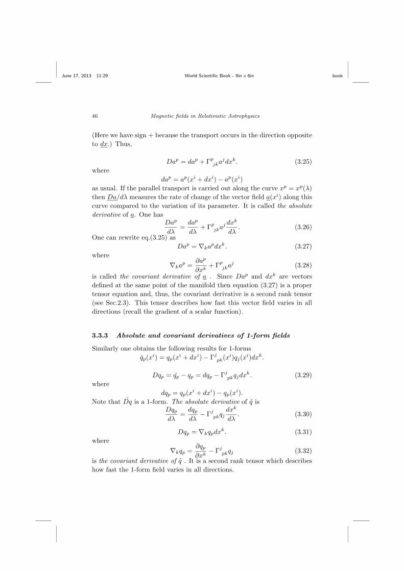
June 17, 2013 11:29 World Scientific Book - 9in x 6in book
46 Magnetic fields in Relativistic Astrophysics
(Here we have sign + because the transport occurs in the direction opposite
to dx.) Thus,
Dap = dap + Γpjkajdxk. (3.25)
where
dap = ap(xi + dxi)− ap(xi)as usual. If the parallel transport is carried out along the curve xp = xp(λ)
then Da/dλ measures the rate of change of the vector field a(xi) along this
curve compared to the variation of its parameter. It is called the absolute
derivative of a. One hasDap
dλ=dap
dλ+ Γpjka
j dxk
dλ. (3.26)
One can rewrite eq.(3.25) as
Dap = ∇kapdxk. (3.27)
where
∇kap =∂ap
∂xk+ Γpjka
j (3.28)
is called the covariant derivative of a . Since Dap and dxk are vectors
defined at the same point of the manifold then equation (3.27) is a proper
tensor equation and, thus, the covariant derivative is a second rank tensor
(see Sec.2.3). This tensor describes how fast this vector field varies in all
directions (recall the gradient of a scalar function).
3.3.3 Absolute and covariant derivatives of 1-form fields
Similarly one obtains the following results for 1-forms
qp(xi) = qp(x
i + dxi)− Γjpk(xi)qj(xi)dxk.
Dqp = qp − qp = dqp − Γjpkqjdxk. (3.29)
where
dqp = qp(xi + dxi)− qp(xi).
Note that Dq is a 1-form. The absolute derivative of q isDqpdλ
=dqpdλ− Γjpkqj
dxk
dλ. (3.30)
Dqp = ∇kqpdxk. (3.31)
where
∇kqp =∂qp∂xk− Γjpkqj (3.32)
is the covariant derivative of q . It is a second rank tensor which describes
how fast the 1-form field varies in all directions.

June 17, 2013 11:29 World Scientific Book - 9in x 6in book
Geometry of Riemannian manifolds 47
3.3.4 Absolute and covariant derivatives of general tensor
fields
The similar procedure applies to higher rank tensors. For example, for the
field of second rank tensor T ij one has
DT ijdλ
= ∇mT ijdxm
dλ(3.33)
where
∇mT ij =∂T ij∂xm
+ ΓikmTkj − ΓkjmT
ik, (3.34)
whereas for the third rank tensor T ijs
DT ijsdλ
= ∇mT ijsdxm
dλ(3.35)
∇mT ijs =∂T ijs∂xm
+ ΓikmTkjs − ΓkjmT
iks − ΓksmT
ijk. (3.36)
These examples illustrate the general formal rules
• The absolute derivative of a tensor field of rank r is a tensor or rank r;
• The covariant derivative of a tensor field of rank r is a tensor or rank
r + 1;
• The first term in the expression for the covariant derivative is the usual
partial coordinate derivative (∂/∂xm) of tensor’s components;
• There are r more terms in this expression, one per each index. In each
such term for an upper index this index is treated as a vector index
and in each such term for a lower index it is treated as a 1-form index.
There many different notations for partial and covariant derivatives.
The most common of the them are described below.
1) ∂mai ≡ ai,m ≡
∂ai
∂xm. (3.37)
2) ai;m ≡ ∇mai. (3.38)
3) ai;m ≡ ∇mai = gmkai;k ≡ gmk∇kai. (3.39)

June 17, 2013 11:29 World Scientific Book - 9in x 6in book
48 Magnetic fields in Relativistic Astrophysics
3.3.5 General properties of covariant differentiation
It is easy to show that the covariant differentiation has the following familiar
properties:
∇m(A+B) = ∇mA+∇mB, (3.40)
and
∇m(AB) = (∇mA)B +A(∇mB), (3.41)
where multiplication can be both inner and outer. Although the actual
number and position of indexes of A and B do not matter here (this is
why their indexes are not shown) the general rules of tensor equations still
apply. For example,
∇m(Aij +Bij) = ∇mAij +∇mBij ,
∇m(AiBi) = (∇mAi)Bi +Ai(∇mBi),
∇m(AiBj) = (∇mAi)Bj +Ai(∇mBj),
3.3.6 The field of metric tensor
Since
gij = gij
(see Sec.3.2.4) one has
Dgijdλ
= 0 (3.42)
along any curve and hence
∇mgij = 0. (3.43)
3.4 Divergence
The divergence of vector field is defined via
divA = ∇mAm. (3.44)

June 17, 2013 11:29 World Scientific Book - 9in x 6in book
Geometry of Riemannian manifolds 49
Obviously this is a scalar. Similarly one defines the divergence of higher
rank tensors; in all cases the index of differentiation is contracted with one
of the indexes of the differentiated tensor. For example,
divT = ∇mTmki. (3.45)
The result is a tensor, whose rank is less than the rank of the differentiated
tensor by one. The notation divT is not particularly informative because
it does not tell which index of tensor T is involved in the contraction. For
this reason it is not widely used.
In applications, one is often interested in how the divergence relates
to partial derivatives with respect to the coordinates of utilised coordinate
system. Here we derive such expressions for vectors and symmetric second
rank tensors. First, we show that
Γiji =∂ ln
√|g|
∂xj, (3.46)
where g is the determinant of the matrix, (gij), constracted out of the
components of the metric tensor. Although g in any coordinate system is
given by a single number, this number is not the same and thus g is not a
scalar. The total differential of g relates to the differentials of gij via
dg =∑i
Aij0dgij
0,
where Aij0 is the minor of (gij) corresponding to the element gij0. Note
that the index j0 is not dummy. This result immediately follows from the
... . On the other hand, the matrix of (gij) is inverse to (gij) and therefore
gij =Ajig.
Combining the last two results and using the symmetry of the metric tensor
we obtain the useful result
dg = ggikdgik. (3.47)
From Eq.3.14 we have
Γl il =1
2
(glj
∂gij∂xl
+ glj∂gjl∂xi− glj ∂gil
∂xj
).
It is easy to see that the first and the second terms are opposite and, thus,
Γl il =1
2glj
∂gjl∂xi
,

June 17, 2013 11:29 World Scientific Book - 9in x 6in book
50 Magnetic fields in Relativistic Astrophysics
According to Eq.3.47 we can write this result as
Γl il =1
2g
∂g
∂xi,
which leads straight to Eq.3.46.
Now we derive the desired expressions for the divergence of vectors and
symmetric second rank tensors. Using Eq.3.28 one can write
∇iai =∂ai
∂xi+ Γiika
k,
and using Eq.3.46 to rewrite this as
∇iai =∂ai
∂xi+∂ ln
√|g|
∂xiai,
which can be simplified as
∇iai =1√|g|
∂√|g|ai
∂xi. (3.48)
In Cartesian coordinates of Euclidean space |g| = 1 and Eq.3.48 simplifies
to the familiar
∇iai =∂ai
∂xi.
Now consider the antisymmetric tensor F ij . According to the rules of
covariant differentiation (see Sec.3.3.4) we have
∇iF jk =∂F jk
∂xi+ ΓjimF
mk + ΓkimFjm, (3.49)
and, thus,
∇iF ik =∂F ik
∂xi+ ΓiimF
mk + ΓkimFim.
Since F im is antisymmetric and Γkim is symmetric with respect to indexes
i and m, the last term in this expression vanishes and, using Eq.3.46, it can
be written as
∇iF ik =∂F ik
∂xi+ Fmk
∂ ln√|g|
∂xm.
Thus, we obtain the same expression as for the divergence of vectors
∇iF ik =1√|g|
∂√|g|F ik
∂xi. (3.50)

June 17, 2013 11:29 World Scientific Book - 9in x 6in book
Geometry of Riemannian manifolds 51
In general case, however, the expression for the divergence of second
rank tensor does not have such a simple form. For example, consider the
symmetric tensor Tij. Then
∇iT jk =∂T jk∂xi
+ ΓjimTmk − ΓmikT
jm,
and
∇iT ik =∂T ik∂xi
+ ΓiimTmk − ΓmikT
im.
The first two terms in this equation combine as before to give
1√|g|
∂√|g|T ik∂xi
.
The last term, however, gives
1
2gmjT im
(∂gij∂xk
+∂gjk∂xi
− ∂gik∂xj
)=
1
2T ij
(∂gij∂xk
+∂gjk∂xi
− ∂gik∂xj
)=
1
2T ij
∂gij∂xk
.
Combining these results we finally obtain
∇iT ik =1√|g|
∂√|g|T ik∂xi
− 1
2T ij
∂gij∂xk
. (3.51)
3.5 Geodesics and parallel transport
We already know (see Sec.1.4) that geodesics are solutions of the Euler-
Lagrange equations
d
dλ
∂L
∂xk− ∂L
∂xk= 0 (k = 1, 2, ..., n) (3.52)
with Lagrangian
L(xk, xk) = gij xixj . (3.53)
(Recall that xk = dxk/dλ where λ is a normal parameter of the geodesic.)
It easy to see that
∂L
∂xk=∂gij∂xk
xixj and∂L
∂xk= 2gikx
i.

June 17, 2013 11:29 World Scientific Book - 9in x 6in book
52 Magnetic fields in Relativistic Astrophysics
Substitution of these results into eq.(3.52) gives us
d
dλ(2gikx
i)− ∂gij∂xk
xixj = 0.
⇒ 2∂gik∂xj
xj xi + 2gikxi − ∂gij
∂xkxixj = 0.
⇒ gikxi +
1
2
(∂gik∂xj
+∂gjk∂xi
− ∂gij∂xk
)xixj = 0.
Now we can use eq.(3.12) and write this result as
gikxi + Γkij x
ixj = 0.
By raising index k (see eq.3.14 and eq.2.48) this is turned into the so-called
geodesic equation
xk + Γkij xixj = 0 (3.54)
which is the same as
Dti
dλ= 0, (3.55)
where
ti =dxi
dλ(3.56)
is the tangent vector to the geodesic. In other words, the tangent vector ti is
the same along the geodesic in the absolute sense ( in the sense of parallel
transport along the geodesic). This results allows to give the following
alternative definition of a geodesic curve
Definition. A curve is called geodesic if it allows a parameter λ such
that
Dti
dλ= 0, where ti =
dxi
dλ
Such parameter is called “normal” and ti is called ” the normal tangent vec-
tor”. It is this property of geodesics that is meant when they are described
as the straightest possible curves.
June 17, 2013 11:29 World Scientific Book - 9in x 6in book
Geometry of Riemannian manifolds 53
3.6 Geodesic coordinates and Fermi coordinates
3.6.1 Geodesic coordinates
By definition, for any point of a Riemannian manifold one can find such a
system of coordinates, called locally Cartesian that at this point
gij =
{1 if i = j
0 if i 6= j(3.57)
Moreover, for any point of a Riemannian manifold one can find such a
system of coordinates that
Γijk = 0, (3.58)
and, hence,
gij,k = 0; (3.59)
∇m =∂
∂xm; (3.60)
D
dλ=
d
dλ. (3.61)
at this particular point. Such coordinates are call geodesic coordinates.
Here is how geodesic coordinates coordinates can be set up. Select a
point on the manifold where the conditions (3.58-3.61) are to be satisfied.
At this point, introduce a set of basis vectors, {ei}, which will become the
coordinate basis of geodesic coordinates. Select a neighbourhood, Np , of
P such that for any point A ∈ Np there exists one and only one geodesic
connecting it to P . Let λ be such a normal parameter of this geodesic that
λ = 0 at P . Denote as u = d/dλ its tangent vector at P and as λA the
value of λ at A. Then the geodesic coordinates of point A are defined via
xiA = uiλA. (3.62)
Obviously, there many normal parameters which satisfy the above selection
criteria and we need to show that the result is the same for any of them.
Consider another such normal parameter, µ. Then
µ = cλ where c = const

June 17, 2013 11:29 World Scientific Book - 9in x 6in book
54 Magnetic fields in Relativistic Astrophysics
and the new tangent vector
vi =dxi
dµ=
1
c
dxi
dλ.
Thus,
xiA = viµA =1
cuicλA = uiλA.
Next we need to show that in these coordinates the Christoffel symbols
vanish at the point P. From eq.(3.62) it follows that all geodesics passing
through P satisfy
xi = uiλ where ui = const, (3.63)
which ensures
xi = 0.
Given this result the geodesic equation (3.54) reads
Γijkxj xk = 0.
Thus, that for any vector ui at point P
Γijkujuk = 0
which can only be satisfied if
Γijk = 0.
Geodesic coordinates are very convenient for many analytical calcula-
tions.
3.6.2 Fermi coordinates
In Euclidean space equations (3.58-3.61) are satisfied throughout the whole
space when we employ Cartesian coordinates (or coordinates related to
the Cartesian ones via linear transformation.) For general Riemannian
manifolds it in impossible to find such coordinates that equations (3.58-
3.61) are satisfied throughout the whole manifold. The most what can be
achieved in general is to get them satisfied along a given geodesic. The
corresponding coordinates are called Fermi coordinates.
Here is the way of constructing such coordinates. First we select a
geodesic curve with normal parameter λ such that at point O ,the origin

June 17, 2013 11:29 World Scientific Book - 9in x 6in book
Geometry of Riemannian manifolds 55
of the Fermi coordinates, λ = 0 (we shell call it the Fermi geodesic). At
this point select such a basis {ei} that e1 = d/dλ. Parallel transport this
basis (along the Fermi geodesic) to every other point of the Fermi geodesic.
Select such a neighbourhood of the Fermi geodesic, N , that for any point
A ∈ N there exists one and only one geodesic with normal tangent vector
u = d/dµ which connects this point to some point P of the Fermi geodesic
so that u = uiei with u1 = 0 at P . Choose such normal parameter µ that
µ = 0 at P. The Fermi coordinates of the point A are then defined as
x1 = λPxi = µAu
i i = 2, . . . , n.(3.64)
In these coordinates the Fermi geodesic satisfies the equation
d2xi
dλ2= 0
and the geodesic through A satisfies
d2xi
dµ2= 0.
This ensures that for any geodesic through P
Γijkxj xk = 0
which can only be satisfied if
Γijk = 0.
Fermi coordinates play important role in the theory of relativity. They
correspond to the so-called free-falling frames.

June 17, 2013 11:29 World Scientific Book - 9in x 6in book
56 Magnetic fields in Relativistic Astrophysics
3.7 Riemann curvature tensor
Parallel transport on Riemannian manifolds has a number of properties not
seen in Euclidean space. This is clearly demonstrated in the following ex-
amples involving a 2D sphere. Recall that any vector tangent to a geodesic
remains tangent during parallel transport along this geodesic. Moreover,
since the angle between two parallel transported vectors is constant so must
be the angle between a vector parallel transported along a geodesic and this
geodesic.
(1) The result of parallel transport depends not only on the initial and final
points but also on the path along which this transport is carried out!
(a) When vector t is parallel transported from the point A on the equa-
tor to the north pole, N , along the meridian AN the result is vector
t′;
(b) When vector t is first parallel transported from the point A to the
point C along the equator, which results in vector t∗, and then
parallel transported from C to N along the meridian CN the result
is a different vector, t′′ 6= t′.
(2) Parallel transport along a closed curve does not result in the original
vector!
Indeed, when vector t′ is parallel transported along the closed path
NACN the result is vector t′′
Obviously these peculiar properties stem from the fact that sphere is
a curved surface! Curvature of such surfaces and general manifolds is de-
scribed via the so called Riemann curvature tensor.

June 17, 2013 11:29 World Scientific Book - 9in x 6in book
Geometry of Riemannian manifolds 57
• Consider a manifold M and a point A ∈ M. Select vectors a, dx(1),
and dx(2) defined at A. Introduce local coordinates {xi} and construct the
close path ABCDA as shown in the figure.
Parallel transport vector a along this path (first in the direction of dx(1))
to obtain vector a+da at point A. Since this path is infinitesimally small ~da
must depend linearly on ~a, ~dx(1), and ~dx(2) and vanish if ~a = 0 or ~dx(1) = 0
or ~dx(2) = 0. That is we must have
dai = Rilmpaldxm(1)dx
p(2). (3.65)
Since this is a proper tensor equation, Rilmp is a tensor and it is called the
Riemann curvature tensor. Direct calculations show that
Rklmp = −Γklm,p + Γklp,m − ΓslmΓkps + ΓslpΓkms (3.66)
(Note that although Γijk is not a tensor, Rkijl is(!) Such peculiar results
do occur from time to time.)
• Curvature of manifolds also causes deviation of initially parallel
geodesics. Consider two infinitesimally close points, A and B, separated
by the infinitesimal displacement vector dx.
Select some vector t at A and parallel transport it from A to B along ~dx.
Construct two geodesics passing through A and B with normal parameter
µ. Namely, the geodesic xi = xi(A)(µ) such that
µ = 0 anddxi
dµ= tiat A
and the geodesic xi = xi(B)(µ) such that
µ = 0 anddxi
dµ= tiat B.

June 17, 2013 11:29 World Scientific Book - 9in x 6in book
58 Magnetic fields in Relativistic Astrophysics
These geodesics can be described as parallel at points A and B. Denote
the displacement vector separating the points of these two geodesics which
have the same value of µ as
sdλ where dλ = const.
One can show that
Dsi
dµ= Riljkt
ltjsk ≡ Riljkdxl
dµ
dxj
dµsk. (3.67)
This equation in called the equation of geodesic deviation. It shows that
initially parallel geodesics deviate from each other.
In Cartesian coordinates of Euclidean space all Γijk = 0 and from (3.66)
one has
Rijkl = 0.
Since R is a tensor, this is true in any basis ( R is just a zero tensor.) Thus,
all dai in (3.65) and all Dsi/dµ in (3.67) vanish and we recover the familiar
properties of Euclidean space.
Definition A manifold is called internally flat (often just flat) if every-
where on this manifold Rijkl = 0, otherwise it is called internally curved.
For example planes and cylinders of Euclidean space are internally flat
manifolds (surfaces).
• One can also show that
(∇m∇p −∇p∇m)ak = Rklmpal; (3.68)
(∇m∇p −∇p∇m)ak = −Rlkmpal. (3.69)
Thus, on curved manifolds the operators of covariant differentiation do not
commute.

June 17, 2013 11:29 World Scientific Book - 9in x 6in book
Geometry of Riemannian manifolds 59
3.8 Properties of the Riemann curvature tensor
• Rijkl has a number of properties which reduce the number of its inde-
pendent components:
Rpijk = −Rpikj ; (3.70)
Rpijk = −Ripjk; (3.71)
Rpijk = Rjkpi; (3.72)
Rppij = 0; (3.73)
Rpijk +Rpjki +Rpkij = 0. (3.74)
Note the cyclic permutation of the lower indexes in eq.(3.74). The best way
of proving these properties involves use of geodesic coordinates. Indeed,
since in geodesic coordinates Γijk = 0 and gij,k = 0, eq.(3.66) has a much
simpler form
Rklmp = −Γklm,p + Γklp,m . (3.75)
Using eq.(3.12) this can also be written as
Rklmp =1
2[gkp,lm + glm,kp − gkm,lp − glp,km] (3.76)
(By the way, eq.(3.76) tells us that all second order derivatives of gij vanish
only if Rijkl = 0!) Now it easy to see that, for example,
Rklmp = −Γklm,p+Γklp,m = −(Γklm,p−Γklp,m) = −(−Γklp,m+Γklm,p) = Rklpm,
which proves eq.(3.70).
Because of the properties (3.70-3.74) the curvature tensor has only
N =1
12n2(n2 − 1)
independent components (the total number of components is n4, where n
is the dimension of the manifold.) If n = 2 then N = 1. The curvature
tensor of 2D manifolds has only one independent component.
• One can also show (using geodesic coordinates once again) that
Rikpl;m +Riklm;p +Rikmp;l = 0 (3.77)
(Note the cyclic permutation of indexes p, l,m in this equation.) This result
is known as the Bianchi identity.

June 17, 2013 11:29 World Scientific Book - 9in x 6in book
60 Magnetic fields in Relativistic Astrophysics
3.9 Ricci tensor, curvature scalar and the Einstein tensor
These important tensors are derived from the Riemann curvature tensor.
The Ricci tensor is defined via
Rij = Rsisj (3.78)
The symmetries (3.70-3.72) ensue that
Rij = −R si sj = −Rsijs = R s
si j , (3.79)
as well as
Rij = Rji. (3.80)
The curvature scalar is defined as
R = Rii. (3.81)
The Einstein tensor is
Gij = Rij −1
2Rgij . (3.82)
It is easy to see
Gij = Gji. (3.83)
Moreover, using the Bianchi identity one can show that
Gik;k ≡ ∇kGsk ≡ 0. (3.84)
In other words, the divergence of Einstein’s tensor is zero.

June 17, 2013 11:29 World Scientific Book - 9in x 6in book
PART 2
Basic Theory of Relativity
61
June 17, 2013 11:29 World Scientific Book - 9in x 6in book
62

June 17, 2013 11:29 World Scientific Book - 9in x 6in book
Chapter 4
Space and time in the theory ofrelativity
Each physical theory is based on a number of key assumptions - the rest of
the theory is then build on these assumptions using appropriate mathemat-
ical tools. Any good theory has to be self-consistent (no internal contradic-
tions) and consistent with Nature. It seems like the second condition can
never be achieved completely. As we learn more we discover new, previously
unknown contradictions between our theories and Nature. They force us
to revise our theories by constructing new sets of basic assumptions. What
was revised during the transition from from Newtonian physics to General
Relativity are the assumptions on the nature of physical time and space.
4.1 Space and Time in Newtonian Physics
4.1.1 Time
Newtonian physics assumes that time is absolute, in the sense that simul-
taneity of events and their durations are the same for all observers. If
events A and B are simultaneous for you then they are simultaneous for
everyone else. If event A takes 2 seconds for you then it takes 2 seconds
for anyone else, provided absolutely accurate standard clocks are used. In
physical terms simultaneity would be easy to establish if there there were
signals that propagate with infinite speed so when an event occurs in a
remote place you one be aware of it instantaneously. Thus, time can be
measured by a single standard clock. From the mathematical viewpoint
this allow to introduce t as universal parameter to describe motion evolu-
tion and interaction in the Universe.
63

June 17, 2013 11:29 World Scientific Book - 9in x 6in book
64 Magnetic fields in Relativistic Astrophysics
4.1.2 Space
It also assumes that physical space is absolute, in the sense that sizes of
physical objects and distances between them, as measured at a particu-
lar time, are the same for all observers equipped with absolutely accurate
standard tools for measuring length. This space is not evolving in time. Its
geometry is Euclidean and thus one can introduce Cartesian coordinates
covering the whole of physical space.
4.1.3 Inertial frames
In order to describe motion/evolution of physical systems we need to have a
system of spatial coordinates at any time. The way this is done in practice
can be rather complicated. In theory one introduces a spatial grid with
known distances between its nodes. These distances do not have to be
fixed and thus the grid can move in space in a certain convenient way. Such
spatial grid is called a reference frame. Depending of the problem under
consideration some of these references frames are better than others as they
provide a simple description of the studied phenomena. In particular, the
motion of free particles has a particularly simple form when described in
so-called inertial frames where they move with constant speed:
Dvi
dt= 0, (4.1)
where
vi =dxi
dtor v =
d
dt.
One can think of an inertial frame as a collection of free particles moving
with the same speed, so that the distances between them are fixed, the
grid of spatial coordinates being attached to these particle. These spatial
coordinates do not have to be Cartesian – the use of the absolute derivative
in eq.4.1 ensures that the choice of spatial coordinates is not important.
Since eq.4.1 in nothing else but the geodesic equation, trajectories of free
particles in Newtonian mechanics are straight lines (geodesic of Euclidean
space). The absolute time t is a normal parameter of this geodesic, and
vi = dxi/dt is its tangent vector.
In Cartesian coordinates eq.4.1 can be written as
dvi
dt= 0, or
d2xi
dt2= 0.
June 17, 2013 11:29 World Scientific Book - 9in x 6in book
Space and time in the theory of relativity 65
4.1.4 Newtonian principle of relativity:
There are infinitely many inertial frames moving relative to each other. If a
body is at rest in one inertial frame it will appear in motion in other frames.
Thus, the notion of mechanical motion appears relative. In fact, the laws
of Newtonian mechanics are exactly the same for all inertial frames making
impossible to decide which of the frames is at rest in space. However, the
absolute nature of space in Newtonian physics implies that the notion of
absolute motion, that is the motion relative to the absolute space, is mean-
ingful and that such motion can be detected by studing physical phenomena
outside of the realm of mechanics.
4.2 Space and Time in Special Relativity
4.2.1 Spacetime
Various experiments show that in vacuum electromagnetic waves propagate
with the same speed, c, relative to all inertial observers. Moreover, c is the
maximum possible speed for any signal. This result is in conflict with the
Galilean transformation between inertial frames, which is the direct result
of the assumptions of Newtonian physics on the nature of space and time.
If one accepts it then the theory of space and time has to be changed.
First, the invariance of the speed of light implies that time can no longer
be considered as absolute. Events simultaneous in one inertial frame be-
come time-separated in others. Different inertial observers measure differ-
ent time intervals between the same events even if they use identical clocks
and procedures. Thus, each inertial frame of Special Relativity has to be
attributed with its own time.
Second, physical space cannot be considered as absolute too. Different
inertial observers obtain different results when they measure lengths of the
same objects even if they use identical standard meters and identical pro-
cedures. Mathematically, this means that this space can not be described
as a metric space.
However, for any two event separated by the time interval ∆t and dis-
tance ∆l their combination
∆s2 = −c2∆t2 + ∆l2, (4.2)
called the spacetime interval, is invariant for all inertial observers even if
∆t and ∆l are not. This shows that physical time and space can be united

June 17, 2013 11:29 World Scientific Book - 9in x 6in book
66 Magnetic fields in Relativistic Astrophysics
into a single 4-dimensional metric space, called spacetime, with ∆s being
the generalised distance between its points, called events. One can see
straight away that this generalised distance is rather peculiar as ∆s2 can
be both positive and negative. In fact, if ∆s2 > 0 then there exists a frame
where ∆t = 0 and ∆s2 = ∆l2. Such spacetime intervals are called space-
like. If ∆s2 < 0 then there exists a frame where ∆l = 0 and ∆s2 = −c2∆t2.
Such spacetime intervals are called time-like. Thus, the possibility of both
positive and negative ∆s2 reflects the underlying difference between space
and time. Spacetime intervals such that ∆s2 = 0 are called null. They
cannot be reduced to either pure space or pure time intervals. (If fact they
describe events on the world-line of a light signal.)
Conventionally, the indexes of spacetime coordinated are shown using
Greek aphabet. Moreover, they run not from 1 to 4 but from 0 to 3,
reserving 0 for the time-like dimension and 1,2,3 for the space-like dimen-
sions (denoted using Latin alphabet). However, one can always introduce
such curvilinear coordinates in spacetime that some coordinate lines change
their type from time-like to space-like and the other way around. In such
coordinates, the nature of dimensions can no longer be reflected in their
indexation.
If {xν} are arbitrary coordinates of the spacetime then the interval
between its infinitesimally close points is given by the metric form
ds2 = gµνdxµdxν where µ, ν = 0, 1, 2, 3. (4.3)
Inertial frames correspond to special cordinate systems of spacetime,
which are postulated to exist. In these coordinate systems the spacetime
metric reduces to
ds2 = −(dx0)2 + gijdxidxj i, j = 1, 2, 3, (4.4)
where gij do not depend on x0. Here x0 = ct, there t is the global time
of the inertial frame and xi (i = 1, 2, 3) are its spatial coordinates. The
hyper-surface x0 =const has positive-definite metric form
dl2 = gijdxidxj i, j = 1, 2, 3, (4.5)
and corresponds to the space of this inertial frame. Moreover, it is assumed
that one can introduce such global spatial coordinates xi that
dl2 = (dx1)2 + (dx2)2 + (dx3)2

June 17, 2013 11:29 World Scientific Book - 9in x 6in book
Space and time in the theory of relativity 67
throughout the whole hypesurface x0 =const. This means that this hyper-
surface is a 3-dimensional Euclidean space.
Thus, the spacetime of Special Relativity allows coordinates {xν} such
that
ds2 = −(dx0)2 + (dx1)2 + (dx2)2 + (dx3)2 (4.6)
and, hence,
gµν =
−1 0 0 0
0 1 0 0
0 0 1 0
0 0 0 1
(4.7)
throughout the whole spacetime. These coordinates are called pseudo-
Cartesian. Metric spaces which allow such coordinates are called pseudo-
Euclidean or Minkowskian.
The scalar product of a non-zero vector uν with itself in such a space,
gνµuνuµ, can be positive, negative, or zero. Thus, similarly to the clas-
sification of the spacetime intervals spacetime vectors can be classified as
space-like, time-like, or null. In order to distinguish between vectors of
space-time and the usual spacial vectors we agree to reserve the notation v
for the spatial vectors (3-vectors) and use −→u for the vectors of space-time
(4-vectors).
4.2.2 Special principle of relativity
Since the absolute space is no longer introduced in Special Relativity the
notion of absolute motion become obsolite as well and all all physical laws
must be exactly the same in all inertial frames. This is known as the Special
Relativistic Principle of Relativity. The Introduction of spacetime allows us
to transform this principle into a simple prescription for writing relativistic
laws of physics. To see this, return for a moment to Newtonian physics.
It is assumed there that, at least in principle, all physical phenomena can
be studied without interfering with them. In particular, their development
does not depend on the choise of spatial coordinate system. Thus, the laws
of physics can be expressed either in the form that does not involve coor-
dinates, or in the form that is exactly the same for all sorts of coordinates.
One example of the first form is the vector (and tensor) equations, like
Dvi
dt= 0

June 17, 2013 11:29 World Scientific Book - 9in x 6in book
68 Magnetic fields in Relativistic Astrophysics
or
Dv
dt= 0.
The correponding example of the second form is the vector (and tensor)
equations written in components, like
dvi
dt+ Γijkv
jvk = 0.
Since in Special Relativity different inertial frames correspond to dif-
ferent systems of coordinates in spacetime, this suggests to use the same
approach. Namely, to express physical laws as tensor equations involv-
ing tensors of spacetime (4-tensor equations), including vector and scalar
equations as special cases of tensor equations.
For example, consider the motion of free particles. In spacetime each
particle traces a curve which is called its world-line. To parametrize this
curve introduce the particle’s proper time, τ , which is the time measured
in the frame where this particle is at rest (This definition makes the proper
time a spacetime scalar.). The spacetime vector
~u =d
dτor uν =
dxν
dτ(4.8)
tangent to the world-line is called the particles 4-velocity. In the local
inertial frame comoving with the particle t = τ , x0 = ct, and xi = const,
and thus uν = (c, 0, 0, 0). This allows us to calculate
|~u|2 = gνµuνuµ = −c2. (4.9)
Thus, 4-velocity is a time-like vector. Now consider the following equation
Duν
dτ= 0. (4.10)
Since this is a 4-vector equation, and hence complies with the Special Prin-
ciple of Relativity, it may constitute a law of physics. In components, this
equation reads
duν
dτ+ Γνµηu
µuη = 0. (4.11)
where Γνµη are the Christoffel symbols of spacetime. In the pseudo-
Cartesian coordinates of any inertial frame Γνµη = 0 and Eq.4.11 yields
duν
dτ= 0 or uν = const. (4.12)

June 17, 2013 11:29 World Scientific Book - 9in x 6in book
Space and time in the theory of relativity 69
Thus,
cdt
dτ= const and
dxi
dτ= const,
which gives us
dxi
dt= const or
dvi
dt= 0, (4.13)
where vi = dxi/dt is the usual 3-velocity of the particle. Since in Cartesian
coordinates D/dt = d/dt the last result can be written as the 3-vector
equation
Dvi
dt= 0, (4.14)
which states that the 3-velocity does not change. Notice that the inertial
frame we used here is arbitrary and that the result (4.14) holds in all inertial
frames. Clearly it describes the motion of free particles and thus Eq.4.10
is the relativistic law law of motion of free particles.
4.3 Space and Time in General Relativity
4.3.1 Spacetime
The key idea of General Relativity is that gravitational interaction makes
itself felt via producing internal curvature of spacetime. The following
example from Newtonian mechanics helps to understand this idea. Consider
the motion of particles bound to a spherical surface but otherwise free of
any force. Such particle simply move along geodesics of the sphere (with
constant speed). These geodesics are great circles. Consider two such
particles initially located on the equator with parallel and equal initial
velocities. As they move in the direction of the north pole they accelerate
toward each other as if they were under the action of a mutual attraction
force.
The spacetime is no longer assumed to be a flat pseudo-Euclidean space
but instead a curved pseudo-Riemannian manifold. The fact that it is only a
manifold implies that topologically it can be different from a 4-dimensional
space and one may not be able to introduce global coordinates covering the
whole of spacetime. The classification as pseudo-Riemannian means that

June 17, 2013 11:29 World Scientific Book - 9in x 6in book
70 Magnetic fields in Relativistic Astrophysics
for any point of spacetime one can introduce local coordinates such that at
this point
gµν =
−1 0 0 0
0 1 0 0
0 0 1 0
0 0 0 1
. (4.15)
4.3.2 General principle of relativity
The key assumption of General Relativity is that it is not possible to de-
tect the effects of gravitational interaction via local measurements. In other
words, experiments carried out within a sufficiently small free-falling labora-
tory can not detect the presence of nearby gravitating bodies. For example,
the astronauts on board of a space station orbiting the Earth and the as-
tronauts on board of a spacecraft coasting far away from Earth, in almost
empty deep space, share exactly the same experiences, e.g. weightlessness.
This implies that all local physical laws, that is laws formulated in terms
of quantities defined at a single point of spacetime, must have exactly the
same form as in the flat spacetime of Special Relativity. In particular,
the Riemann curvature tensor can not appear in these equations with the
exception of the equations of gravitational field which show how exactly
the curvature is imposed on spacetime. For example, the motion of free
particles is still described by
Duµ
dτ= 0,
which implies that their world lines are still geodesics of spacetime.
4.3.3 Locally inertial frames
There are no global inertial frames in General Relativity. Indeed, the curva-
ture of spacetime, inflicted by gravitational interactions, does not allow us
to introduce global pseudo-Cartesian coordinates. If we could the spacetime
would be a Minkowskian space. However, the general relativistic principle
of relativity implies that one should be able to built locally inertial frames
in which all local physical phenomena occure in the same fasion as Special
Relativity. They should correspond to such system of spacetime coordi-
nates in which all physical laws take exactly the same form as in Special

June 17, 2013 11:29 World Scientific Book - 9in x 6in book
Space and time in the theory of relativity 71
Relativity but only locally that to introduce local pseudo-Cartesian coordi-
nates such that in small volume of space-time its metric is very close to that
of flat pseudo-Eucledean space. The locally pseudo-Cartesian coordinates
satisfying Eq.4.15 correspond to a frames which close to inertial for a short
period of time within a small volume. One can also introduce local geodesic
coordinates which not only satisfy Eq.4.15 but also ensure that
Γνµη = 0 (4.16)
at the selected point (normally the origin). These are even better candi-
dates to be associated with locally inertial frames. Finally, for any time-like
geodesic one can introduce the system of Fermi coordinates such that both
Eq.4.15 and Eq.4.16 are satisfied along this geodesic. These coordinates
correspond to a small free-falling laboratory with its almost Euclidean spa-
cial grid covering the volume of the lab and its standard system of time
keeping. Within the small volume of such a laboratory the effects of finite
curvature of spacetime are very small.
4.4 Relativistic particle dynamics
Denote as m the particle’s mass as measured in the comoving inertial frame.
It will be called the rest mass of the particle. This definition insures that
the rest mass is a spacetime scalar (4-scalar), and hence it value does not
depend on the choice of spacetime coordinates used to describe particle’s
motion. The 4-vector
P ν = muν , (4.17)
where uµ is the particle’s 4-velocity, is called the energy-momentum or the
4-momentum vector of the particle. Obviously,
|~P |2 = m2|~u|2 = −m2c2 < 0, (4.18)
and, thus, this 4-vector is time-like. Consider, an arbitrary local inertial
frame and a system of local pseudo-Cartesian coordinates assosiated with
this frame. Denote the time and space components of this 4-vector in the
coordinate basis as E/c and pi, that is
P ν = (E/c, p1, p2, p3). (4.19)
Obviously,
E = mγc2 (4.20)

June 17, 2013 11:29 World Scientific Book - 9in x 6in book
72 Magnetic fields in Relativistic Astrophysics
and
pi = mγvi, (4.21)
where vi are the components of the particle’s 3-velocity in this frame. At
speeds much less compared to the speed of light If we introduce new pa-
rameter,
m = mγ, (4.22)
called the inertial mass of the particle. Then laboratory frame. From
eq.(4.13) it follows that for a free particle
E = const and pi = const. (4.23)
Thus, the energy and the momentum of a free particle are conserved. The
4-tensor equation with describes this conservation is
DPµ
dτ= 0. (4.24)
When a particle is subjected to a force its 3-velocity is no longer constant
and neither is its 4-velocity. The appropriate modification of (4.10) is
D(muν)
dτ= fν , (4.25)
where fν is a spacetime vector called the four-force and m is the mass of
the particle as measured in the frame where it is at rest. Hence the name,
the “rest mass”. This definition ensures m is the same for all inertial frames
and, hence, that m is a spacetime scalar.
If the case of the electromagnetic force
fν =q
cF νµuµ, (4.26)
where q is the electric charge of the particle (a spacetime scalar), and F νµ
is the electromagnetic field tensor.
4.5 Conservation laws
Consider a continuous medium that can be attributed with some scalar
quantity M of volume density ρ. The amount of M within volume V is
then
M =
∫V
ρdV

June 17, 2013 11:29 World Scientific Book - 9in x 6in book
Space and time in the theory of relativity 73
Vector ~J is called the flux density of M if ~J · ~dS gives us the flux of
M across the surface element ~dS in the direction shown by ~dS, that is the
amount of M passing through the surface element per unit time. The total
amount of M leaving volume V is then simply
∫δV
J · dS =
∫δV
J idSi,
where δV is the surface of V and ~dS is its outgoing surface element.
Fig. 4.1 Integration volume V , its surface element dS, and the flux density vector J .
If M is not created or destroyed inside V then the amount of M in this
volume varies only due to the flow of M out of V into the outside space.
Hence, we have
d
dt
∫V
ρdV = −∫δV
J · dS
or
d
dt
∫V
ρdV +
∫δV
J · dS = 0. (4.27)
This is the integral form of the conservation law for the scalar quantity M
with volume density ρ and flux density ~J . According to the Gauss theorem
one can rewrite this as
d
dt
∫V
ρdV +
∫V
∇iJ idV = 0
and, thus, ∫V
(∂ρ
∂t+∇iJ i
)dV = 0.
Since the volume V is arbitrary we deduce from this that
∂ρ
∂t+∇iJ i = 0, (4.28)
which is called the differential form of the conservation law for scalar quan-
tity M with volume density ρ and flux density ~J .

June 17, 2013 11:29 World Scientific Book - 9in x 6in book
74 Magnetic fields in Relativistic Astrophysics
If replace M with a vector quantity then in the place of ρ we should
have a vector, e.g. P , and in the place of ~J we should have a tensor, e.g.
T ij . The integral conservation law will then look as
d
dt
∫V
P idV +
∫δV
T ijdSj = 0. (4.29)
and the differential one as
∂P i
∂t+∇jT ij = 0. (4.30)
Notice, that eq.4.30 is a proper tensor equation whereas eq.4.29 is not
because it involves addition of components of vectors defined at different
points of space.
Sometimes it is relatively easy to figure out the flux density. For ex-
ample, consider a swarm of particles of mass m, number density n and
3-velocity ~v as measured in some inertial frame. Suppose that the number
of particles is conserved. Then the total mass of the swarm will also be
conserved. During the time interval (t, t+ dt) the only particles that cross
the surface ~dS are these that occupy at time t the oblique cylinder shown
below.
Fig. 4.2
Its volume is
dV = v⊥ dt dS = (v · dS)dt;
the total number of particles in this volume is dN = ndV and the total
mass is dM = mndV . Thus, the total mass carried through the surface dS
during the time interval dt is
dM = nm(v · dS)dt.
This shows that the mass flux density is
J = nmv. (4.31)
4.6 Relativistic continuity equation
Consider a swarm of particles moving with four-velocity uν . Let n be the
number density of these particles as measured in the inertial frame moving

June 17, 2013 11:29 World Scientific Book - 9in x 6in book
Space and time in the theory of relativity 75
with the same velocity as the local velocity of the swarm. It is called the
proper number density. Consider the following 4-tensor equation
∇ν(nuν) = 0. (4.32)
Here ∇ν is the operator of covariant differentiation in spacetime. Notice
that n is a spacetime scalar, ∇µ(nuν) is a spacetime tensor, and hence
∇ν(nuν) is a spacetime scalar. Thus, equation (4.32) is a proper tensor
equation and may express a physical law (see the principle of relativity).
But what law? In the pseudo-Cartesian coordinates of an arbitrary inertial
frame, laboratory frame,
∇ν =∂
∂xνand uν = γ(c, v1, v2, v3) (4.33)
where γ is the Lorentz factor and vi is the usual velocity vector (three-
vector). Thus, (4.32) reads
∂
∂x0(γcn) +
∂
∂xi(γnvi) = 0 (4.34)
Since x0 = ct and in Cartesian coordinates
∇i =∂
∂xi
this can also be written as
∂
∂t(γn) +∇i(γnvi) = 0 (4.35)
or
∂
∂t(n) +∇i(nvi) = 0 (4.36)
where n = γn is the number density of particles as measured in the lab-
oratory frame, it is different from n because of the Lorentz contraction.
(Notice that ∇i is the operator of covariant differentiation in space, the
hypersurface x0 =const.) Obviously, eq.(4.35) describes the conservation
of particles as seen in the laboratory frame and, thus, the 4-tensor equa-
tion (4.32) describes the same conservation but in a coordinate independent
form.
Introduce the proper rest mass density of the swarm,
ρ = mn. (4.37)
Since the rest mass m is a spacetime scalar we can now rewrite (4.32) as
∇ν(ρuν) = 0. (4.38)
This 4-tensor equation is called the relativistic continuity equation.

June 17, 2013 11:29 World Scientific Book - 9in x 6in book
76 Magnetic fields in Relativistic Astrophysics
4.7 Stress-energy-momentum tensor
4.7.1 Stress-energy-momentum tensor of dust
Consider now a swarm of free particles of the proper number density n, the
proper rest mass density ρ = mn, and the 4-velocity uν . The tensor
Tµν = ρuµuν (4.39)
is called the stress-energy-momentum tensor of the swarm. Components of
this tensor also allow simple interpretation. Consider an arbitrary inertial
frame (the laboratory frame). Denote as e the energy density (per unit
volume), as πi the momentum density and as si the energy flux density of
the swam in this frame. Then
e = T 00, πi = (1/c)T 0i = (1/c)T i0, si = cT 0i = cT i0. (4.40)
Moreover, T ij if the momentum flux density, the stress 3-tensor. (T ij gives
us the flux density of the i-component of momentum in the j-direction, and,
at the same time, the flux density of the j-component of momentum in the
i-direction.) Indeed,
•
e = ρu0u0 = ργ2c2 = (mγc2)(nγ) = En; (4.41)
•
πi = ρu0ui/c = ργ2vi = (mγvi)(nγ) = pin; (4.42)
•
si = cρu0ui = ργ2c2vi = evi; (4.43)
•
T ij = ρuiuj = (ργ2vi)vj = πivj ; (4.44)
and
T ij = ρuiuj = (ργ2vj)vi = πjvi. (4.45)
Thus, like the usual energy and momentum of a single particle are simply
components of a first rank 4-tensor ( energy-momentum vector), the usual
energy density, momentum density, energy flux density and stress tensor
(3-tensor) of a continuously distributed system are components of a second
rank 4-tensor (stress-energy-momentum tensor).

June 17, 2013 11:29 World Scientific Book - 9in x 6in book
Space and time in the theory of relativity 77
4.7.2 Energy-momentum conservation
Consider the following equation
∇νTµν = 0. (4.46)
Since this is a 4-tensor equation it may express some physical law. But
what law? In the pseudo-Cartesian coordinates of the laboratory frame
∇µ =∂
∂xµ. (4.47)
Thus, eq.(4.46) reads
∂
∂xνTµν = 0 (4.48)
or
∂
∂x0Tµ0 +
∂
∂xiTµi = 0 (4.49)
or
1
c
∂
∂tTµ0 +
∂
∂xiTµi = 0. (4.50)
The time component of this equation (µ = 0) can be written as
∂
∂te+∇isi = 0. (4.51)
This is just the energy conservation law. The spatial component (µ =
1, 2, 3) of eq.(4.50) reads as
∂
∂tπj +∇iT ji = 0. (4.52)
This is just the momentum conservation law. Thus eq.(4.46) describes the
conservation of energy and momentum in a coordinate independent form.
4.7.3 Stress-energy-momentum tensor of perfect fluid
Any continuous system like a fluid or a force field can be attributed with
its own stress-energy-momentum tensor and if this system is isolated (does
not interact with other systems) then eq.(4.46) is satisfied.
Let us determine the stress-energy-momentum tensor of ideal fluid.
What we need is an expression for this 4-tensor in terms of lower rank
(more basic) 4-tensors like in eq.(4.39). But it is easier to figure out the
components of T ij in the rest frame of the fluid. (By this we mean the
inertial frame where the fluid is at rest. Obviously, each fluid element has

June 17, 2013 11:29 World Scientific Book - 9in x 6in book
78 Magnetic fields in Relativistic Astrophysics
it own rest frame.) In the rest frame the energy per unit volume is given
by
T 00 = e = ρc2 + ε,
their ρ is the rest mass density and ε is the thermal energy density. More-
over, since vi = 0 the momentum density and hence the energy flux density
vanish in this frame
πi = T 0i = T i0 = 0.
The components of stress tensor of ideal fluid at rest in Cartesian coordi-
nates are
T ij =
p 0 0
0 p 0
0 0 p
where p is the thermodynamic pressure. Thus, in the pseudo-Cartesian
coordinates of the rest frame the components of stress-energy momentum
tensor of ideal fluid are
Tµν =
e 0 0 0
0 p 0 0
0 0 p 0
0 0 0 p
. (4.53)
Note that e and p are spacetime scalars. They completely determine the
thermodynamical state of ideal fluid. Its motion is completely determined
by the 4-vector uν . Thus, what we need to do now is to construct T νµ from
e, p, and uν via suitable tensor operations in such a way that in the fluid
frame we end up with eq.(4.53). In fact,
Tµν = (e+ p
c2)uµuν + pgµν (4.54)
does the job. Indeed, in the pseudo-Cartesian coordinates of the rest frame
of the fluid
uν = (c, 0, 0, 0)
gµν =
−1 0 0 0
0 1 0 0
0 0 1 0
0 0 0 1
,
and eq.(4.54) reduces to eq.(4.53).

June 17, 2013 11:29 World Scientific Book - 9in x 6in book
Space and time in the theory of relativity 79
4.8 Einstein’s equations of gravitational field
Let us speculate on how the equations of gravitational field could look like.
Obviously they must be tensor equations and should involve the Riemann
curvature tensor. If this curvature is caused by matter then some tensor
fields describing the distribution of matter must also be involved.
In Newtonian gravity matter is present in the form of its volume mass
density. But in relativistic physics things are different in two respects:
(1) Mass is attributed not only to matter but also to force fields (like the
electromagnetic field) via m = E/c2. This suggests that not only mat-
ter but also force field can curve spacetime.
(2) The volume mass density (or energy density) is not a spacetime scalar
but just one component of the stress-energy-momentum tensor. This
suggests to seek a simple tensor equation relating the Riemann curva-
ture tensor with T νµ, the total stress-energy-momentum tensor!
The metric tensor may also be present in this equation because of it
fundamental role in geometry. However, the equation must agree with the
symmetries of involved tensors. It does not seem possible to relate T νµ and
gµν with Rνµηπ directly. For example, the equation
Rνµηπ = agµνTηπ
is in conflict with the symmetries of the Riemann curvature tensor (eqs.3.70-
3.74). However, the Ricci tensor has the same rank and the same symmetry
as T νµ and initially Einstein suggested that
Rνµ = aT νµ,
where a is a constant. However, he quickly realised that this is no good.
Indeed, because
∇µRνµ 6= 0
one ends up with
∇µT νµ 6= 0
which contradicts to the general principle of relativity. So, Einstein sug-
gested another equation which is free from such a flaw, namely
Gνµ = aT νµ, (4.55)
where Gνµ = Rνµ− (R/2)gνµ is now known as the Einstein tensor. Indeed,
as we have already seen (equation 3.84),
∇µGνµ ≡ 0

June 17, 2013 11:29 World Scientific Book - 9in x 6in book
80 Magnetic fields in Relativistic Astrophysics
implying
∇µT νµ = 0. (4.56)
Equation (4.55) is known as the Einstein equation of gravitational field.
Later we shell see that
a =8πG
c4(4.57)
The Einstein equation (4.55) is the key equation of General Relativity.
Once this equation is introduced we can forget all the reasons which have
led Einstein to this equation and simply derive from it all the important
results of the Theory of Relativity. For example, as we have already seen,
equation (4.56) follows directly from the Einstein equation. This equation
describes the dynamics of continuous media like fluids and fields. For a
swarm of dust particles
Tµν = ρuµuν , (4.58)
where ρ = mn is the rest mass density of the swarm (see Sec.4.5.2). Hence,
eq.(4.56) reads
∇νTµν = ∇νρuνuµ = ρuν∇νuµ + uµ∇νρuν = 0. (4.59)
Since these particle do not interact with each other their total number is
conserved and we have
∇νρuν = 0. (4.60)
This allows us to write eq.(4.59) as
ρuν∇νuµ = 0,
or
Duν
dτ= 0.
This is the equation of motion of free particles (geodesic motion).
Now we may consider a time-like geodesic of a free falling laboratory and
construct the corresponding system of Fermi coordinates of this geodesic.
Since in these coordinates
Γνµη = 0D
dt=
d
dtand ∇ν =
∂
∂xν

June 17, 2013 11:29 World Scientific Book - 9in x 6in book
Space and time in the theory of relativity 81
along the geodesic (notice that here τ = t) the equations of continuous
dynamics, (4.56) and (4.60) reduce to
∂
∂xµT νµ = 0,
and
∂
∂xµρuµ = 0,
and the equation of geodesic motion reduces to
duν
dt= 0.
This is exactly how they read in the pseudo-Cartesian coordinates of flat
spacetime. Thus, gravity “disappears” in free falling locally inertial frames.
Einstein’s equation can be written in slightly different form which we
shell use later on. To obtain this, we first contract (eq.4.55)
Gνν = aT νν or Rνν −1
2Rδνν = aT νν
Next we denote
T νν as T (4.61)
and use that δνν = 4 to obtain
R = −aT. (4.62)
Finally, substitute this into (4.55) to obtain
Rνµ = a(T νµ − 1
2Tgνµ). (4.63)
We know that components of the Riemann curvature tensor in the co-
ordinate basis are functions of Γνµη and Γνµη,β . We also know that Γνµηare functions of gνµ and gνµ,β . Thus, the components of Rµνηγ , and hence
the components of Rνµ and Gνµ, depend on the components of gνµ and
their first and second partial derivatives. Thus, the Einstein equations can
be viewed as second order partial differential equations for the components
of the metric tensor! The total number of independent equations in this
system is 10 ( Do you know why?) The same is the total number of inde-
pendent components of the metric tensor. What a match! However, rather
complicated analysis of the Einstein equations shows that they include only
6 evolution equations that describe the “time-evolution” of gµν . Others may
be consider as differential constrains on the initial solution (like ∇ ~B = 0 in
electrodynamics). Thus, there in no match after all and the system appears

June 17, 2013 11:29 World Scientific Book - 9in x 6in book
82 Magnetic fields in Relativistic Astrophysics
to be under-determined. In fact, this is good news! Indeed, the components
of metric tensor depend not only on the structure of the spacetime but also
on the system of coordinates we choose. When we introduce four coordi-
nates in spacetime we effectively impose four additional conditions on the
components of metric tensor. And in reverse, an introduction of four ad-
ditional conditions on the components of metric tensor amounts to setting
up a coordinate system. Here is two examples of such conditions:
• The conditions
g00 = −1, gi0 = 0.
define the so-called “time-orthogonal coordinates” (they may not exist).
• The conditions
gµνΓβµν = 0, which ensure ∇µ∇µxβ = 0,
introduce the so-called “harmonic coordinates”.
Often one cannot give a clear physical interpretation of coordinates intro-
duced in such a way (e.g. one cannot tell which coordinate is time-like and
which are space-like). Only after the Einstein equations are solved and the
functions gνµ(xβ) are found such an interpretation becomes possible.
In fact, the Einstein equations are local and do not tell anything about
the spacetime topology. We have to make explicit assumptions on the
topology of spacetime – for example, we may assume that it has the same
topology as a 4-dimensional sphere of a 5-dimensional Euclidean space. But
will this be a correct assumption?

June 17, 2013 11:29 World Scientific Book - 9in x 6in book
Space and time in the theory of relativity 83
4.9 Newtonian limit
The Newtonian theory of gravity has been extremely successful. It describes
the motion of planets and satellites with great accuracy. This means that in
the limit of low velocities and hence weak gravity any good theory of gravity
must reduce to the Newtonian theory. Let us check that the Einstein theory
satisfies this condition.
Here is the basic equations of the Newtonian theory.
• The equation of motion (the second law of particle mechanics):
~a = −~∇Φ orDvi
dt= −∇iΦ, (4.64)
where ~v is the particle velocity, ~a is the particle acceleration, and Φ is
the gravitational potential.
• The equation of gravitational field:
∆Φ = 4πGρ, (4.65)
where ρ is the mass density, G is the gravitational constant, and
∆ = ∇i∇i = gij∇i∇j
is the Laplace operator.
In Cartesian coordinates {xi} these equations read
dvi
dt= − ∂Φ
∂xi(4.66)
and
3∑i=1
∂2Φ
∂xi2 = 4πGρ. (4.67)
The basic equations of the Einstein theory are
• The equation of motion:
Duν
dτ= 0, (4.68)
• The field equation:
Rµν = a(Tµν −1
2Tgµν). (4.69)
What are the conditions of weak gravity?

June 17, 2013 11:29 World Scientific Book - 9in x 6in book
84 Magnetic fields in Relativistic Astrophysics
(1) The curvature of spacetime must be very small. Thus, there must be
possible to construct such a system of coordinates that the metric tensor
has almost the same components as in flat spacetime (Minkowskian) in
pseudo-Cartesian coordinates. That is
gµν = ηµν + hµν , (4.70)
where
ηµν =
−1 0 0 0
0 1 0 0
0 0 1 0
0 0 0 1
, (4.71)
and
|hµν | � 1. (4.72)
(2) Moreover, the particle velocity must be much lower than the speed of
light. Hence, we may assume
u0 = c, and |ui| � c. (4.73)
This ensures that the proper time of the particle, τ , is very close to the
coordinate time t = x0/c:
τ = t. (4.74)
Moreover, given such low characteristic speeds
∂
∂x0≈(vc
) ∂
∂xi� ∂
∂xi. (4.75)
(3) Finally, for a nonrelativistic thermal motion (low temperatures)
ρc2 � ε, p. (4.76)
This means that only the rest mass of gravitating objects makes any no-
ticeable contribution to their stress-energy-momentum tensors. Thus,
the gravitational field is fully determined by the distribution of rest
mass.
Conditions (4.73) and (4.76) show that the T00 component of the Tµνtensor is much larger than all other components and we may assume that
Tµν =
ρc2 0 0 0
0 0 0 0
0 0 0 0
0 0 0 0
(4.77)

June 17, 2013 11:29 World Scientific Book - 9in x 6in book
Space and time in the theory of relativity 85
with great accuracy.
Let us check if under these conditions the Einstein equations (4.68) and
(4.69) reduce to the Newtonian equations (4.66) and (4.67). Let us start
with the equation of motion. Using (4.74) one can write the spatial part of
(4.68) as
dui
dt+ Γiµνu
µuν = 0.
Using (4.73) this can be written as
dui
dt+ Γi00c
2 = 0. (4.78)
From (3.12) we have
Γαµν =1
2gαγ
[∂gγµ∂xν
+∂gγν∂xµ
− ∂gµν∂xγ
].
Substituting gνµ from (4.70-4.72) and keeping only the terms first order in
h we obtain
Γαµν =1
2ηαγ
[∂hγµ∂xν
+∂hγν∂xµ
− ∂hµν∂xγ
], (4.79)
which gives us
Γi00 =1
2ηiγ[∂hγ0∂x0
+∂hγ0∂x0
− ∂h00∂xγ
].
Since ηνµ is diagonal we have
Γi00 =1
2ηii[∂hi0∂x0
+∂hi0∂x0
− ∂h00∂xi
]=
1
2
[∂hi0∂x0
+∂hi0∂x0
− ∂h00∂xi
].
Finally, using (4.75) we may ignore the derivative with respect to x0 and
obtain
Γi00 = −1
2
∂h00∂xi
. (4.80)
Then eq.(4.78) reads
dui
dt=c2
2
∂h00∂xi
. (4.81)
Notice that this equation has exactly the same form as (4.66). This suggests
to relate h00 with Newtonian gravitational potential via
Φ = −c2
2h00. (4.82)

June 17, 2013 11:29 World Scientific Book - 9in x 6in book
86 Magnetic fields in Relativistic Astrophysics
Let us now deal with the field equation. From eq.(4.77) we find
T00 = ρc2 and T = T νν = T 00 = η00T00 = −ρc2.
Thus, the time component of (4.69) reads
R00 =a
2ρc2. (4.83)
Equation (4.79) shows that all components of Γ are small (of order
O(h)). Keeping only terms linear in Γ we can write
Rαβγδ =∂
∂xγΓαβδ −
∂
∂xδΓαβγ
(see eq.3.66) and thus
R00 = Rα0α0 =∂
∂xαΓα00 −
∂
∂x0Γα0α.
Once again we may ignore derivatives with respect to x0 and obtain
R00 =∂
∂xiΓi00.
Substitution of Γi00 from (4.80) into this equation gives us
R00 = −1
2
3∑i=1
∂2h00
∂xi2 .
Thus, equation (4.83) reads
−1
2
3∑i=1
∂2h00
∂xi2 =
a
2ρc2. (4.84)
Using eq.(4.82) we can write this as3∑i=1
∂2Φ
∂xi2 =
ac4
2ρ. (4.85)
This equation has exactly the same form as the Newtonian field equation
(4.67). Thus, Einstein’s equations do reduce to the Newtonian equations
indeed! Moreover, now we can express constant a of the Einstein equations
in terms the gravitational constant, G, and the speed of light:
a =8πG
c4. (4.86)

June 17, 2013 11:29 World Scientific Book - 9in x 6in book
Chapter 5
Schwarzschild Solution
In this chapter we study a particular solution of Einstein’s equations that
describes the spacetime outside of a spherically symmetric non-rotating
body of a certain mass, e.g. a non-rotating black hole, and the motion
of test particles in such spacetime. Throughout this chapter we use the
relativistic units, also known as the geometric units, where G = 1 and
c = 1.
5.1 Schwarzschild Solution
5.1.1 Schwarzschild Solution in Schwarzschild coordinates
The interval of pseudo-Euclidean spacetime of special relativity in pseudo-
Cartesian coordinates is given by
ds2 = −dt2 + dx2 + dy2 + dz2
For problems with spherical symmetry in space (t =const hypersurface) it
is more convenient to use spherical spatial coordinates {r, θ, φ}. Then the
spacetime interval takes the following form:
ds2 = −dt2 + dr2 + r2(dθ2 + sin2 θdφ2).
Now, let us try to come up with a simple and reasonable expression for
the metric form of the spacetime about a stationary spherically symmetric
body of total mass m. When we say “stationary” we mean that it must be
possible to introduce such a reference frame that the spatial location of the
body remains fixed forever. In such frame the components of metric tensor
cannot depend on time t. (Far away from the body this t must tick at the
same rate as the proper time of observers at rest relative to mass m. )
87

June 17, 2013 11:29 World Scientific Book - 9in x 6in book
88 Magnetic fields in Relativistic Astrophysics
If the body is spherically symmetric then we expect the spacetime to
be spherically symmetric as well. Therefore, like in Euclidean space, we
should be able to introduce spatial coordinates {r, θ, φ} such that the line
element depends on the angles θ and φ only via the combination
dθ2 + sin2 θdφ2.
Thus, we expect the metric form to have the following structure
ds2 = −a(r,m)dt2 + b(r,m)dr2 + c(r,m)r2(dθ2 + sin2 θdφ2). (5.1)
There three unknown functions, they are a(r,m), b(r,m), and c(r,m), in
this expression1. It can be reduced to two, if we redefine r via
(r′)2 = c(r,m)r2.
Then, (5.1) reads
ds2 = −A(r,m)dt2 +B(r,m)dr2 + r2(dθ2 + sin2 θdφ2) (5.2)
where we have omitted ′, or
gµν =
−A(r,m) 0 0 0
0 B(r,m) 0 0
0 0 r2 0
0 0 0 r2 sin2 θ
.
Far away from this body we expect the curvature gradually reduce to
zero. In other words, we expect the spacetime to become flat at spatial
infinity, that is
A,B → 1 as r →∞. (5.3)
In fact we can impose even more restrictive constraint on A(r,m). Indeed,
given the results of Sec.4.9, we may assume that far away from the body
A = 1− htt = 1 + 2Φ = 1− 2m/r. (5.4)
(Here htt is the same as h00 in Sec.4.9)1Notice that we introduced more than 4 additional constraints on the components of
metric tensor assuming the metric form (5.1) (see the discussion at the end of Sec.4.8)

June 17, 2013 11:29 World Scientific Book - 9in x 6in book
Schwarzschild Solution 89
This is how we think the metric tensor should look like in some suitable
coordinates {t, r, θ, φ}. It remains to be seen that Einstein’s equations do
indeed allow solutions of this form. The required computations are carried
out as follows: (i) compute gµν,γ , (ii) then gµν,γδ, (iii) then Rµνγδ, (iv) then
Rµν , (v) then Gµν . To find the solution describing spacetime outside of the
body we need to substitute the result into the vacuum version of Einstein’s
equations:
Gνµ = 0.
This gives us a system of second order ordinary differential equations for
A(r,m) and B(r,m) (note that m is a parameter, not a variable.) which
we need to solve subject to conditions at infinity. The general solution of
those equation is
A(r,m) = a(m)− b(m)/r,
B(r,m) = c(m)/A(r,m).
Conditions (5.3,5.4) are satisfied by A(r,m) if
a(m) = 1, b(m) = 2m,
and the condition (5.3) is satisfied if
c(m) = 1.
Thus, the final result is
ds2 = −(1− 2m/r)dt2 + (1− 2m/r)−1dr2 + r2(dθ2 + sin2 θdφ2) (5.5)
or
gµν = 0 if ν 6= µ
gtt = −(1− 2m/r), grr = (1− 2m/r)−1, gθθ = r2, gφφ = r2 sin2 θ.
This solution is known as the Schwarzschild solution and the coordinates
{t, r, θ, φ} are called the Schwarzschild coordinates. If the radius of the body
is r∗ then it holds only for r > r∗. However, the Schwarzschild solution also
describes the spacetime of a black hole – in such case it applies for r > 0. To
be more precise, this solution applies only to non-rotating objects. Rotation
inflicts additional curvature on spacetime.

June 17, 2013 11:29 World Scientific Book - 9in x 6in book
90 Magnetic fields in Relativistic Astrophysics
Let us analyse the nature of the Schwarzschild coordinates.
• For any r > 0
gθθ =~∂
∂θ·~∂
∂θ> 0, gφφ =
~∂
∂φ·~∂
∂φ> 0
and, thus, θ and φ are space-like coordinates.
• For r > 2m
gtt =~∂
∂t·~∂
∂t< 0, grr =
~∂
∂r·~∂
∂r> 0
and, thus, t is a time-like coordinate and r is a space-like one as ex-
pected.
• However, for r < 2m
gtt =~∂
∂t·~∂
∂t> 0, grr =
~∂
∂r·~∂
∂r< 0
and, thus, r is a time-like coordinate and t is a space-like one. Hence
the lesson: Do not assume that the coordinate denoted as t always
refers to time measurements! Be prepared to unexpected!
One can see that r = 0 is special. gtt and grr →∞ as r → 0. In fact, the
curvature scalar R also tends to∞. At this point the curvature of spacetime
becomes infinite. This is a real spacetime singularity of the Schwarzschild
solution – the place where the approximation of General Relativity breaks
down.
5.1.2 Schwarzschild Solution in Kerr coordinates
r = 2m is also rather special as grr → ∞ as r → 2m. However, R re-
mains finite and hence the curvature of spacetime is finite. There is no
spacetime singularity on this surface. In fact, on this surface the system
of Schwarzschild coordinates becomes singular. It is possible to introduce
other coordinate systems that are free from such singularity. One example
is the system of Kerr coordinates which is introduced as follows:
• r, θ, and φ are the same as in Schwarzschild coordinates,
• New t′ = t′(t, r) coordinate is introduced via the following transforma-
tion, singular at r = 2m:
dt′ = dt− (1− r/2m)−1dr, (5.6)

June 17, 2013 11:29 World Scientific Book - 9in x 6in book
Schwarzschild Solution 91
or
∂t′
∂t= 1
∂t′
∂r= (1− r/2m)−1
Notice that Maxwell’s integrability condition
∂2t′
∂t∂r=
∂2t′
∂r∂t
is satisfied by the transformation (5.6)
Substitution of dt from (5.6) into (5.5) gives
ds2 = −(1−2m/r)dt′2 +(4m/r)dt′dr+(1+2m/r)dr2 +r2(dθ2 +sin2 θdφ2).
(5.7)
One can see that now all components of the metric tensor are finite at
r = 2m and, thus, there is no singularity there. Moreover, now the r-
coordinate is always space-like. Notice, that eqs.(5.5) and (5.7) describe
the same spacetime (In what follows we will no longer use ′ to indicate
Kerr’s time.)
5.1.3 Event horizon
Is it always possible to have a physical object, say a test particle, at rest
relative to a black hole, that is with fixed r, θ, φ coordinates? The spacetime
interval along the world-line of any particle is negative
ds2 = −dτ2,
where τ is the proper time of the particle. For a stationary particle
dr = dθ = dφ = 0
and, thus, along its world-line one has
ds2 = −(1− 2m/r)dt2
which is negative if r > 2m and positive if r < 2m. Thus, no stationary
particle, as well as no stationary physical observer, can exist at r < 2m!
If inside r = 2m particles must be moving then what kind of motion
is it? It is easy to see that all terms on the right side in eq.(5.7) are non-
negative if r < 2m except the second one, which may both positive and
negative. Hence, if ds2 is negative then so must be this second term. This
means
drdt < 0 and, hence, dr/dt < 0.

June 17, 2013 11:29 World Scientific Book - 9in x 6in book
92 Magnetic fields in Relativistic Astrophysics
Thus the particle is forced to move inwards, toward the physical singu-
larity at r = 0. The critical radius rg = 2m is called the gravitational or
Schwarzschild radius (in generic units rg = 2Gm/c2) and the surface r = rgis called the event horizon as nothing can escape from inside of this surface
into the outside space. Whatever event occurs inside the event horizon the
outside observers are not receiving any information about it.
Exercise
Determine the distance Lhs between the horizon and the singularity
along the radial direction of Kerr coordinates (t, θ, φ = const).
Solution: In Kerr coordinates
~∂
∂r·~∂
∂r= grr = 1 + 2m/r > 0
and, thus, along the radial direction
ds2 = dl2 = grrdr2 > 0.
This is a space-like direction. Hence,
Lhs =
r=2m∫r=0
dl =
2m∫0
√grrdr =
2m∫0
√1 + 2m/rdr
If we introduce new variable y =√r/2m then
Lhs = 4m
1∫0
√1 + y2dy.
Given that ∫ √1 + y2dy =
1
2
[y√
1 + y2 + ln(y +√
1 + y2)]
we finally obtain
Lhs = 2m[√
2 + ln(1 +√
2)].
June 17, 2013 11:29 World Scientific Book - 9in x 6in book
Schwarzschild Solution 93
5.2 Gravitational redshift
Consider the Schwarzschild solution in Schwarzschild coordinates:
ds2 = −(1− 2m/r)dt2 + (1− 2m/r)−1dr2 + r2(dθ2 + sin2 θdφ2). (5.8)
Consider an observer at rest (dr = dθ = dφ = 0) at infinity. If τ∞ is the
proper time of this observer then
dτ2∞ = −ds2 = dt2. (5.9)
Thus, the coordinate t that selects the spacetime hypersurface t = const
may be interpreted as the time measured by an observer at rest at infinity
by means of a standard clock.
Consider another observer at rest at 2m < r <∞. His/her proper time
is
dτ2r = −ds2 = (1− 2m/r)dt2 (5.10)
and, thus,
dτ2r = (1− 2m/r)dτ2∞ (5.11)
Notice, that dτr < dτ∞. This property is often described as slowing
down of clocks ( or even of time) in gravitational field. In fact, this is exactly
what a distant observer watching a standard clock of another observer,
placed near a gravitating body, will see.
Consider two observers, A and B, resting at r = ra and r = rb re-
spectively (both outside the horizon). The interval of coordinate time δt
required for a light signal emitted by A to reach B does not depend on the
time of emission because the components of metric tensor in Schwarzschild
coordinates do not depend on t. To illustrate this point consider the case
where both observers are situated along the same radial direction (θa = θb,
φa = φb. This simplifies the calculations.) Due to the spherical symme-
try of spacetime the light signal has to propagate along the same radial
direction and the spacetime interval along its world-line is given by
ds2 = gttdt2 + grrdr
2 = 0.
Therefore,
dt2 = (−grr/gtt)dr2

June 17, 2013 11:29 World Scientific Book - 9in x 6in book
94 Magnetic fields in Relativistic Astrophysics
and
δt =
∣∣∣∣∣∣rb∫ra
√(−grr/gtt)dr
∣∣∣∣∣∣ . (5.12)
Since gµν do not depend on t so does not δt.
Suppose A emits two signals separated by the interval ∆t of the coordi-
nate time t. When B receives these signals they are still separated by the
same interval ∆t. Indeed, if they are emitted at t = 0 and ∆t then they
are received at t = δt and ∆t + δt. For the same reason, if A emits a pe-
riodic signal of period ∆t of coordinate time t, B records the same period.
However, the proper time τ measured by standard clocks of the observers
run at rates different from the rate of t. From eq.5.10 one has
∆τ2a = (1− 2m/ra)∆t2, ∆τ2b = (1− 2m/rb)∆t2
and, thus,
∆τ2a =
(1− 2m/ra1− 2m/rb
)∆τ2b . (5.13)
If rb =∞ then we have
∆τ2a = (1− 2m/ra)∆τ2∞. (5.14)
Thus, if A emits a periodic signal with the period of its standard clock then
B at r =∞ will see that this clock runs slower than his/her own standard
clock. Notice, that eq.5.14 has exactly the same form as eq.5.11.
On the other hand, ∆τ could be just a period of a monochromatic
electromagnetic wave emitted by A as measured by his/her standard clock.
Since the frequency of the wave ν = 1/∆τ , we have
ν2a =
(1− 2m/rb1− 2m/ra
)ν2b . (5.15)
If rb > ra then νb < νa. Thus, the frequency of an electromagnetic wave
is decreasing as the wave propagates away from the source of gravity. This
effect is called the gravitational redshift. (Optical lines shift toward the red
part of the spectrum).

June 17, 2013 11:29 World Scientific Book - 9in x 6in book
Schwarzschild Solution 95
5.3 Integrals of motion of free test particles in
Schwarzschild spacetime
By test particles we understand particles of such a small mass that their
gravitational field is negligibly small compared to the field of other involved
objects. Such particles can be used to test the gravitational field created
by those bodies without disturbing them. Hence the name test particles.
In Sec.4.4,4.3 we have learned that the equation of motion of a free particle
isDuα
dτ= 0, (5.16)
and, hence, its world-line is a geodesic of spacetime.
From Sec.3.5 ( just substitute λ with τ) we know that the geodesic
equations can be can be written as the Euler-Lagrange equations
d
dτ
∂L∂uµ
− ∂L∂xµ
= 0 (5.17)
with the Lagrangian
L(xν , uµ) = gαβ(xν)uαuβ . (5.18)
These equations allows us to derive a number of very important results on
the motion of test particles in the Schwarzschild spacetime in a rather easy
way.
• Both in the Schwarzschild and Kerr coordinates
∂gαβ∂t
= 0
and, thus,
∂L∂t
= 0. (5.19)
From (5.17) and (5.19) one has
d
dτ
∂L∂ut
= 0,
and, thus, dL/dut is an integral of motion, which means that it is
constants along the world-line of the particle. In fact,
∂L∂ut
=∂(gνµu
νuµ)
∂ut= 2gtνu
ν = 2ut.

June 17, 2013 11:29 World Scientific Book - 9in x 6in book
96 Magnetic fields in Relativistic Astrophysics
Thus, we conclude that
ut = E = const. (5.20)
At infinity, where both in Schwarzschild and Kerr coordinates the met-
ric attains its Minkowskian form, one has
E = ut = gtνuν = gttu
t = −ut = −γ = −Epmp
(5.21)
where Ep is the energy of the particle as measured by an observer at
rest and mp is the rest mass of the particle. For this reason −E is called
the specific energy at infinity.
• Moreover, both in the Schwarzschild and Kerr coordinates
∂gαβ∂φ
= 0
and, thus,
∂L∂φ
= 0 andd
dτ
∂L∂uφ
= 0. (5.22)
Since
∂L∂uφ
=∂(gνµu
νuµ)
∂uφ= 2gφνu
ν = 2uφ,
we conclude that
uφ = l = const (5.23)
is another integral of motion. It is called the specific angular momentum
at infinity.
• Since gµν depend on r and θ we conclude that ur and uθ are not integrals
of motion!
• However, a test particle with initial uθ = 0 placed in the equatorial
plane, θ = π/2 remains in this plane forever. Since the direction of
the polar axis is not restricted (spherical symmetry!) this result simply
tells us that the motion of free particles in Schwarzschild geometry is
planar.
Let us derive this results. Consider the θ-component of (5.17):

June 17, 2013 11:29 World Scientific Book - 9in x 6in book
Schwarzschild Solution 97
d
dτ
∂L∂uθ− ∂L∂θ
= 0. (5.24)
∂L∂θ
=∂(gνµu
νuµ)
∂θ=∂gφφ∂θ
uφuφ =
=∂(r2 sin2 θ)
∂θuφuφ = 2 cos θ sin θr2(uφ)2.
uφ = gφφuφ =1
gφφl =
l
r2 sin2 θ
Thus,
∂L∂θ
=2 cos θl2
r2 sin3 θ. (∗)
Next,
∂L∂uθ
=∂(gνµu
νuµ)
∂uθ= 2gθνu
ν = 2gθθuθ = 2r2uθ. (∗∗)
Substitution of (*) and (**) into (5.24) gives
d
dτ
(r2dθ
dτ
)− cos θl2
r2 sin3 θ= 0. (5.25)
It is easy to see that θ(τ) = π/2 satisfies this equation. Moreover, this
is the unique solution satisfying the initial conditions
{θ(τ0) = π/2
dθ/dτ(τ0) = 0
(The theorem of uniqueness for second order ODEs.)
Exercise
A meteorite falls radially from rest at infinity into a Schwarzschild black
hole. Show that in Schwarzschild coordinates
ur = −√
2m/r.

June 17, 2013 11:29 World Scientific Book - 9in x 6in book
98 Magnetic fields in Relativistic Astrophysics
Solution
At infinity
ui = 0, γ = 1 and, thus, E = −1.
Since the fall is radial, uθ = uφ = 0, the condition
gµνuµuν = −1
reads
gttutut + grru
rur = −1. (+)
Using E one can eliminate ut from this equation. Indeed,
ut = gttut =1
gttE = − 1
gtt
Thus, eq.(+) reads
gtt1
g2tt+ grru
rur = −1.
Now we can find ur = ur(r):
(ur)2 = −(1 + 1/gtt)/grr = −(1− 1
1− 2m/r)(1− 2m/r) =
= −((1− 2m/r)− 1) = 2m/r.

June 17, 2013 11:29 World Scientific Book - 9in x 6in book
Schwarzschild Solution 99
5.4 Orbits of test particles in the Schwarzschild geometry
Consider the Schwarzschild solution in the Schwarzschild coordinates:
ds2 = −(1− rg/r)dt2 + (1− rg/r)−1dr2 + r2(dθ2 + sin2 θdφ2).
We already know that motion of test particles in the Schwarzschild
spacetime is planar. We can always choose the coordinates in such a way
that the plane of motion becomes the equatorial plane, θ = π/2. Then
uθ = 0 and the condition
gµνuµuν = −1
reads
gttutut + grru
rur + gφφuφuφ = −1. (5.26)
Since
ut = gttut = E/gtt and uφ = gφφuφ = l/gφφ,
eq.(5.26) reads
E2
gtt+
l2
gφφ+ grru
rur = −1.
or
E2 + (1 +l2
gφφ)gtt + grrgtt(u
r)2 = 0. (∗)
For θ = π/2 one has
gφφ = r2, grr = (1− rg/r)−1, gtt = −(1− rg/r),
and eq.(*) reduces to
(ur)2 + (1− rg/r)(1 + l2/r2) = E2.
Thus, we obtain
(ur)2 + Φl(r) = E2, (5.27)
where
Φl(r) = (1− rg/r)(1 + l2/r2) (5.28)
From (5.27) one finds

June 17, 2013 11:29 World Scientific Book - 9in x 6in book
100 Magnetic fields in Relativistic Astrophysics
dur
dτ= −1
2
dΦldr
(5.29)
This explains why Φ is called the effective potential.
In the important case of a circular orbit
ur = 0, anddur
dτ= 0,
and equations (5.27) and (5.29) reduce to
Φl(r) = E2, (5.30)
and
dΦldr
= 0 (5.31)
respectively. These equations can be used to find the constants of motion,
E and l, of circular orbits.
Before we proceed with the analysis of let us briefly review the Newto-
nian results.
Newtonian theory
Similar analysis in Newtonian theory gives
(vr)2 + Φl(r) = E2, (5.32)
where
Φl(r) = 1− rg/r + l2/r2 (5.33)
Let us figure out how the motion of a particle with the specific angular
momentum l looks like in the plane E2 against r. Since E is an integral
of motion the particles move parallel to the r-axis. From (5.32) it
follows that
E2 − Φl(r) ≥ 0
and, thus, their motion is confined within the region above the curve
E2 = Φl(r). Everywhere on this curve vr = 0 but only the extremum
corresponds to a circular orbit (see condition (5.31). All other points
of this curve are turning points.
From this figure it follows that

June 17, 2013 11:29 World Scientific Book - 9in x 6in book
Schwarzschild Solution 101
• No particle with l 6= 0 can ever reach r = 0.
• Particles with E2 > 1 will always escape to infinity, even if their
initial vr < 0.
• Particles with E2 < 1 will move between r− and r+.
Einstein’s theory
Differentiating (5.28) one obtains
dΦldr
=rgr4
[r2 − 2
l2
rgr + 3l2
]Thus, the extrema of Φl are the solutions of
r2 − 2
(l2
rg
)r + 3l2 = 0, (5.34)
The solutions to this quadratic equation are
r± =l2
rg± l√
(l/rg)2 − 3. (5.35)
Thus,
• If l2 > 3r2g then there are two circular orbits with radii r+ and r−,
• If l2 = 3r2g then there is only one circular orbit with the radius
rms = 3rg,
• If l2 < 3r2g then there are no circular orbits.
Once again we can understand the properties of orbits by using the
E2-r plane. The figure below shows the curves E2 = Φl(r) for various
values of l. Notice that now Φl → 0 as r → 0.
From this figure it follows that
• Now there exist trajectories leading directly to singularity. Particles
may be swallowed by a black hole.
• For l2 > 3r2g there exist oscillating orbits, for l2 < 3r2g such orbits
do not exist.
• The circular orbit with r = r+ is stable, whereas the one with r = r−is unstable.
• There are no stable orbits with r < rms = 3rg. The orbit with
r = rms is called “the last stable orbit”.

June 17, 2013 11:29 World Scientific Book - 9in x 6in book
102 Magnetic fields in Relativistic Astrophysics
Exercise 1:
Determine the integrals of motion of circular orbits.
Solution:
From eq.(5.34) one has
l2 =mr2
r − 3m. (5.36)
From eqs.(5.30,5.28,5.36) one has
E2 = Φl(r) = (1− 2m/r)(1 + l2/r2) =
= (1− 2m/r)(1 +m/(r − 3m)) =(r − 2m)2
r(r − 3m).
Thus,
E2 =(r − 2m)2
r(r − 3m). (5.37)
Exercise 2:
A spaceship is orbiting a black hole of mass m. Given that its orbit is
circular one with radius r determine the orbital period as measured by
(i) a passenger of the spaceship, T(i),
(ii) a stationary observer far away from the hole (at infinity), T(ii).
Solution:
(i) The period T(i) is measured by a standard clock carried with the
ship. Its time is the proper time of the ship, τ . Since
uφ =dφ
dτ
one has
T(i) = 2π/uφ.
But
uφ = gφφuφ = l/gφφ =1
r2
(mr2
r − 3m
)1/2
=

June 17, 2013 11:29 World Scientific Book - 9in x 6in book
Schwarzschild Solution 103
=1
r
(m
r − 3m
)1/2
.
Hence,
T(i) = 2πr
(r − 3m
m
)1/2
.
(ii) The period T(ii) is measured by a standard clock at rest at infinity.
It runs with the same rate as t (see Sec.5.2). Hence,
T(ii) =dt
dτT(i) = utT(i).
But
ut = gttut = E/gtt = − 1
1− 2m/r
(− r − 2m√
r(r − 3m)
)=
√r
r − 3m.
Thus,
T(ii) =
√r
r − 3m2πr
√r − 3m
m= 2πr
√r/m.

June 17, 2013 11:29 World Scientific Book - 9in x 6in book
104 Magnetic fields in Relativistic Astrophysics

June 17, 2013 11:29 World Scientific Book - 9in x 6in book
Index
geodesic, 12
105