Astrophysical Sources of Cosmic Rays and Related...
44
June 2009 Astrophysical Sources of Cosmic Rays and Related Measurements with the Pierre Auger Observatory Presentations for the 31st International Cosmic Ray Conference, L´ od´ z , Poland, July 2009 1. Correlation of the highest energy cosmic rays with nearby extragalactic objects in Pierre Auger Observatory data presented by J. D. Hague .... Page 6 2. Discriminating potential astrophysical sources of the highest energy cosmic rays with the Pierre Auger Observatory presented by J. Aublin ....... Page 10 3. Intrinsic anisotropy of the UHECR from the Pierre Auger Observatory presented by Jo˜ao de Mello Neto ........................................... Page 14 4. Ultra-high energy photon studies with the Pierre Auger Observatory presented by P. Homola .................................................... Page 17 5. Limits on the flux of diffuse ultra high energy neutrinos set using the Pierre Auger Observatory presented by J. Tiffenberg ........................... Page 20 6. Search for sidereal modulation of the arrival directions of events recorded at the Pierre Auger Observatory presented by R. Bonino .............. Page 24 7. Cosmic Ray Solar Modulation Studies in the Pierre Auger Observatory presented by H. Asorey ..................................................... Page 28 8. Investigation of the Displacement Angle of the Highest Energy Cosmic Rays Caused by the Galactic Magnetic Field presented by B.M. Baughman . Page 32 9. Search for coincidences with astrophysical transients in Pierre Auger Observatory data presented by Dave Thomas ............................ Page 36 10. An alternative method for determining the energy of hybrid events at the Pierre Auger Observatory presented by Patrick Younk .................. Page 40
Transcript of Astrophysical Sources of Cosmic Rays and Related...

June 2009
Astrophysical Sources of Cosmic Rays
and Related Measurements
with the
Pierre Auger Observatory
Presentations for the31st International Cosmic Ray Conference, Lodz , Poland, July 2009
1. Correlation of the highest energy cosmic rays with nearby extragalacticobjects in Pierre Auger Observatory data presented by J. D. Hague . . . .Page 6
2. Discriminating potential astrophysical sources of the highest energy cosmicrays with the Pierre Auger Observatory presented by J. Aublin . . . . . . . Page 10
3. Intrinsic anisotropy of the UHECR from the Pierre Auger Observatorypresented by Joao de Mello Neto . . . . . . . . . . . . . . . . . . . . . . . . . . . . . . . . . . . . . . . . . . . Page 14
4. Ultra-high energy photon studies with the Pierre Auger Observatorypresented by P. Homola . . . . . . . . . . . . . . . . . . . . . . . . . . . . . . . . . . . . . . . . . . . . . . . . . . . . Page 17
5. Limits on the flux of diffuse ultra high energy neutrinos set using the PierreAuger Observatory presented by J. Tiffenberg . . . . . . . . . . . . . . . . . . . . . . . . . . . Page 20
6. Search for sidereal modulation of the arrival directions of events recordedat the Pierre Auger Observatory presented by R. Bonino . . . . . . . . . . . . . . Page 24
7. Cosmic Ray Solar Modulation Studies in the Pierre Auger Observatorypresented by H. Asorey . . . . . . . . . . . . . . . . . . . . . . . . . . . . . . . . . . . . . . . . . . . . . . . . . . . . .Page 28
8. Investigation of the Displacement Angle of the Highest Energy Cosmic RaysCaused by the Galactic Magnetic Field presented by B.M. Baughman . Page 32
9. Search for coincidences with astrophysical transients in Pierre AugerObservatory data presented by Dave Thomas . . . . . . . . . . . . . . . . . . . . . . . . . . . . Page 36
10. An alternative method for determining the energy of hybrid events at thePierre Auger Observatory presented by Patrick Younk . . . . . . . . . . . . . . . . . . Page 40

PIERRE AUGER COLLABORATION
J. Abraham8, P. Abreu71, M. Aglietta54, C. Aguirre12, E.J. Ahn87, D. Allard31, I. Allekotte1,J. Allen90, J. Alvarez-Muniz78, M. Ambrosio48, L. Anchordoqui104, S. Andringa71, A. Anzalone53,
C. Aramo48, E. Arganda75, S. Argiro51, K. Arisaka95, F. Arneodo55, F. Arqueros75, T. Asch38,H. Asorey1, P. Assis71, J. Aublin33, M. Ave96, G. Avila10, T. Backer42, D. Badagnani6,
K.B. Barber11, A.F. Barbosa14, S.L.C. Barroso20, B. Baughman92, P. Bauleo85, J.J. Beatty92,T. Beau31, B.R. Becker101, K.H. Becker36, A. Belletoile34, J.A. Bellido11, 93, S. BenZvi103,C. Berat34, P. Bernardini47, X. Bertou1, P.L. Biermann39, P. Billoir33, O. Blanch-Bigas33,F. Blanco75, C. Bleve47, H. Blumer41, 37, M. Bohacova96, 27, D. Boncioli49, C. Bonifazi33,
R. Bonino54, N. Borodai69, J. Brack85, P. Brogueira71, W.C. Brown86, R. Bruijn81, P. Buchholz42,A. Bueno77, R.E. Burton83, N.G. Busca31, K.S. Caballero-Mora41, L. Caramete39, R. Caruso50,
W. Carvalho17, A. Castellina54, O. Catalano53, L. Cazon96, R. Cester51, J. Chauvin34,A. Chiavassa54, J.A. Chinellato18, A. Chou87, 90, J. Chudoba27, J. Chye89d, R.W. Clay11,
E. Colombo2, R. Conceicao71, B. Connolly102, F. Contreras9, J. Coppens65, 67, A. Cordier32,U. Cotti63, S. Coutu93, C.E. Covault83, A. Creusot73, A. Criss93, J. Cronin96, A. Curutiu39,
S. Dagoret-Campagne32, R. Dallier35, K. Daumiller37, B.R. Dawson11, R.M. de Almeida18, M. DeDomenico50, C. De Donato46, S.J. de Jong65, G. De La Vega8, W.J.M. de Mello Junior18,
J.R.T. de Mello Neto23, I. De Mitri47, V. de Souza16, K.D. de Vries66, G. Decerprit31, L. delPeral76, O. Deligny30, A. Della Selva48, C. Delle Fratte49, H. Dembinski40, C. Di Giulio49,
J.C. Diaz89, P.N. Diep105, C. Dobrigkeit 18, J.C. D’Olivo64, P.N. Dong105, A. Dorofeev88, J.C. dosAnjos14, M.T. Dova6, D. D’Urso48, I. Dutan39, M.A. DuVernois98, R. Engel37, M. Erdmann40,
C.O. Escobar18, A. Etchegoyen2, P. Facal San Luis96, 78, H. Falcke65, 68, G. Farrar90,A.C. Fauth18, N. Fazzini87, F. Ferrer83, A. Ferrero2, B. Fick89, A. Filevich2, A. Filipcic72, 73,I. Fleck42, S. Fliescher40, C.E. Fracchiolla85, E.D. Fraenkel66, W. Fulgione54, R.F. Gamarra2,
S. Gambetta44, B. Garcıa8, D. Garcıa Gamez77, D. Garcia-Pinto75, X. Garrido37, 32, G. Gelmini95,H. Gemmeke38, P.L. Ghia30, 54, U. Giaccari47, M. Giller70, H. Glass87, L.M. Goggin104,M.S. Gold101, G. Golup1, F. Gomez Albarracin6, M. Gomez Berisso1, P. Goncalves71,
M. Goncalves do Amaral24, D. Gonzalez41, J.G. Gonzalez77, 88, D. Gora41, 69, A. Gorgi54,P. Gouffon17, S.R. Gozzini81, E. Grashorn92, S. Grebe65, M. Grigat40, A.F. Grillo55,
Y. Guardincerri4, F. Guarino48, G.P. Guedes19, J. Gutierrez76, J.D. Hague101, V. Halenka28,P. Hansen6, D. Harari1, S. Harmsma66, 67, J.L. Harton85, A. Haungs37, M.D. Healy95,T. Hebbeker40, G. Hebrero76, D. Heck37, V.C. Holmes11, P. Homola69, J.R. Horandel65,
A. Horneffer65, M. Hrabovsky28, 27, T. Huege37, M. Hussain73, M. Iarlori45, A. Insolia50,F. Ionita96, A. Italiano50, S. Jiraskova65, M. Kaducak87, K.H. Kampert36, T. Karova27,P. Kasper87, B. Kegl32, B. Keilhauer37, E. Kemp18, R.M. Kieckhafer89, H.O. Klages37,M. Kleifges38, J. Kleinfeller37, R. Knapik85, J. Knapp81, D.-H. Koang34, A. Krieger2,
O. Kromer38, D. Kruppke-Hansen36, F. Kuehn87, D. Kuempel36, N. Kunka38, A. Kusenko95, G. LaRosa53, C. Lachaud31, B.L. Lago23, P. Lautridou35, M.S.A.B. Leao22, D. Lebrun34, P. Lebrun87,
J. Lee95, M.A. Leigui de Oliveira22, A. Lemiere30, A. Letessier-Selvon33, M. Leuthold40,I. Lhenry-Yvon30, R. Lopez59, A. Lopez Aguera78, K. Louedec32, J. Lozano Bahilo77, A. Lucero54,
H. Lyberis30, M.C. Maccarone53, C. Macolino45, S. Maldera54, D. Mandat27, P. Mantsch87,A.G. Mariazzi6, I.C. Maris41, H.R. Marquez Falcon63, D. Martello47, O. Martınez Bravo59,
H.J. Mathes37, J. Matthews88, 94, J.A.J. Matthews101, G. Matthiae49, D. Maurizio51, P.O. Mazur87,M. McEwen76, R.R. McNeil88, G. Medina-Tanco64, M. Melissas41, D. Melo51, E. Menichetti51,A. Menshikov38, R. Meyhandan14, M.I. Micheletti2, G. Miele48, W. Miller101, L. Miramonti46,
S. Mollerach1, M. Monasor75, D. Monnier Ragaigne32, F. Montanet34, B. Morales64, C. Morello54,J.C. Moreno6, C. Morris92, M. Mostafa85, C.A. Moura48, S. Mueller37, M.A. Muller18,
R. Mussa51, G. Navarra54, J.L. Navarro77, S. Navas77, P. Necesal27, L. Nellen64,C. Newman-Holmes87, D. Newton81, P.T. Nhung105, N. Nierstenhoefer36, D. Nitz89, D. Nosek26,L. Nozka27, M. Nyklicek27, J. Oehlschlager37, A. Olinto96, P. Oliva36, V.M. Olmos-Gilbaja78,
M. Ortiz75, N. Pacheco76, D. Pakk Selmi-Dei18, M. Palatka27, J. Pallotta3, G. Parente78,E. Parizot31, S. Parlati55, S. Pastor74, M. Patel81, T. Paul91, V. Pavlidou96c, K. Payet34, M. Pech27,
J. Pekala69, I.M. Pepe21, L. Perrone52, R. Pesce44, E. Petermann100, S. Petrera45, P. Petrinca49,A. Petrolini44, Y. Petrov85, J. Petrovic67, C. Pfendner103, R. Piegaia4, T. Pierog37, M. Pimenta71,
T. Pinto74, V. Pirronello50, O. Pisanti48, M. Platino2, J. Pochon1, V.H. Ponce1, M. Pontz42,P. Privitera96, M. Prouza27, E.J. Quel3, J. Rautenberg36, O. Ravel35, D. Ravignani2,

A. Redondo76, B. Revenu35, F.A.S. Rezende14, J. Ridky27, S. Riggi50, M. Risse36, C. Riviere34,V. Rizi45, C. Robledo59, G. Rodriguez49, J. Rodriguez Martino50, J. Rodriguez Rojo9,
I. Rodriguez-Cabo78, M.D. Rodrıguez-Frıas76, G. Ros75, 76, J. Rosado75, T. Rossler28, M. Roth37,B. Rouille-d’Orfeuil31, E. Roulet1, A.C. Rovero7, F. Salamida45, H. Salazar59b, G. Salina49,
F. Sanchez64, M. Santander9, C.E. Santo71, E.M. Santos23, F. Sarazin84, S. Sarkar79, R. Sato9,N. Scharf40, V. Scherini36, H. Schieler37, P. Schiffer40, A. Schmidt38, F. Schmidt96, T. Schmidt41,
O. Scholten66, H. Schoorlemmer65, J. Schovancova27, P. Schovanek27, F. Schroeder37, S. Schulte40,F. Schussler37, D. Schuster84, S.J. Sciutto6, M. Scuderi50, A. Segreto53, D. Semikoz31,
M. Settimo47, R.C. Shellard14, 15, I. Sidelnik2, B.B. Siffert23, A. Smiałkowski70, R. Smıda27,B.E. Smith81, G.R. Snow100, P. Sommers93, J. Sorokin11, H. Spinka82, 87, R. Squartini9,
E. Strazzeri32, A. Stutz34, F. Suarez2, T. Suomijarvi30, A.D. Supanitsky64, M.S. Sutherland92,J. Swain91, Z. Szadkowski70, A. Tamashiro7, A. Tamburro41, T. Tarutina6, O. Tascau36,
R. Tcaciuc42, D. Tcherniakhovski38, D. Tegolo58, N.T. Thao105, D. Thomas85, R. Ticona13,J. Tiffenberg4, C. Timmermans67, 65, W. Tkaczyk70, C.J. Todero Peixoto22, B. Tome71,
A. Tonachini51, I. Torres59, P. Travnicek27, D.B. Tridapalli17, G. Tristram31, E. Trovato50,M. Tueros6, R. Ulrich37, M. Unger37, M. Urban32, J.F. Valdes Galicia64, I. Valino37, L. Valore48,
A.M. van den Berg66, J.R. Vazquez75, R.A. Vazquez78, D. Veberic73, 72, A. Velarde13,T. Venters96, V. Verzi49, M. Videla8, L. Villasenor63, S. Vorobiov73, L. Voyvodic87‡, H. Wahlberg6,
P. Wahrlich11, O. Wainberg2, D. Warner85, A.A. Watson81, S. Westerhoff103, B.J. Whelan11,G. Wieczorek70, L. Wiencke84, B. Wilczynska69, H. Wilczynski69, C. Wileman81, M.G. Winnick11,
H. Wu32, B. Wundheiler2, T. Yamamoto96a, P. Younk85, G. Yuan88, A. Yushkov48, E. Zas78,D. Zavrtanik73, 72, M. Zavrtanik72, 73, I. Zaw90, A. Zepeda60b, M. Ziolkowski42
1 Centro Atomico Bariloche and Instituto Balseiro (CNEA-UNCuyo-CONICET), San Carlos de Bariloche,Argentina
2 Centro Atomico Constituyentes (Comision Nacional de Energıa Atomica/CONICET/UTN- FRBA), Buenos Aires,Argentina
3 Centro de Investigaciones en Laseres y Aplicaciones, CITEFA and CONICET, Argentina4 Departamento de Fısica, FCEyN, Universidad de Buenos Aires y CONICET, Argentina
6 IFLP, Universidad Nacional de La Plata and CONICET, La Plata, Argentina7 Instituto de Astronomıa y Fısica del Espacio (CONICET), Buenos Aires, Argentina
8 National Technological University, Faculty Mendoza (CONICET/CNEA), Mendoza, Argentina9 Pierre Auger Southern Observatory, Malargue, Argentina
10 Pierre Auger Southern Observatory and Comision Nacional de Energıa Atomica, Malargue, Argentina11 University of Adelaide, Adelaide, S.A., Australia
12 Universidad Catolica de Bolivia, La Paz, Bolivia13 Universidad Mayor de San Andres, Bolivia
14 Centro Brasileiro de Pesquisas Fisicas, Rio de Janeiro, RJ, Brazil15 Pontifıcia Universidade Catolica, Rio de Janeiro, RJ, Brazil
16 Universidade de Sao Paulo, Instituto de Fısica, Sao Carlos, SP, Brazil17 Universidade de Sao Paulo, Instituto de Fısica, Sao Paulo, SP, Brazil
18 Universidade Estadual de Campinas, IFGW, Campinas, SP, Brazil19 Universidade Estadual de Feira de Santana, Brazil
20 Universidade Estadual do Sudoeste da Bahia, Vitoria da Conquista, BA, Brazil21 Universidade Federal da Bahia, Salvador, BA, Brazil
22 Universidade Federal do ABC, Santo Andre, SP, Brazil23 Universidade Federal do Rio de Janeiro, Instituto de Fısica, Rio de Janeiro, RJ, Brazil
24 Universidade Federal Fluminense, Instituto de Fisica, Niteroi, RJ, Brazil26 Charles University, Faculty of Mathematics and Physics, Institute of Particle and Nuclear Physics, Prague,
Czech Republic27 Institute of Physics of the Academy of Sciences of the Czech Republic, Prague, Czech Republic
28 Palacky University, Olomouc, Czech Republic30 Institut de Physique Nucleaire d’Orsay (IPNO), Universite Paris 11, CNRS-IN2P3, Orsay, France31 Laboratoire AstroParticule et Cosmologie (APC), Universite Paris 7, CNRS-IN2P3, Paris, France32 Laboratoire de l’Accelerateur Lineaire (LAL), Universite Paris 11, CNRS-IN2P3, Orsay, France
33 Laboratoire de Physique Nucleaire et de Hautes Energies (LPNHE), Universites Paris 6 et Paris 7, ParisCedex 05, France

34 Laboratoire de Physique Subatomique et de Cosmologie (LPSC), Universite Joseph Fourier, INPG,CNRS-IN2P3, Grenoble, France35 SUBATECH, Nantes, France
36 Bergische Universitat Wuppertal, Wuppertal, Germany37 Forschungszentrum Karlsruhe, Institut fur Kernphysik, Karlsruhe, Germany
38 Forschungszentrum Karlsruhe, Institut fur Prozessdatenverarbeitung und Elektronik, Karlsruhe, Germany39 Max-Planck-Institut fur Radioastronomie, Bonn, Germany
40 RWTH Aachen University, III. Physikalisches Institut A, Aachen, Germany41 Universitat Karlsruhe (TH), Institut fur Experimentelle Kernphysik (IEKP), Karlsruhe, Germany
42 Universitat Siegen, Siegen, Germany44 Dipartimento di Fisica dell’Universita and INFN, Genova, Italy
45 Universita dell’Aquila and INFN, L’Aquila, Italy46 Universita di Milano and Sezione INFN, Milan, Italy
47 Dipartimento di Fisica dell’Universita del Salento and Sezione INFN, Lecce, Italy48 Universita di Napoli ”Federico II” and Sezione INFN, Napoli, Italy
49 Universita di Roma II “Tor Vergata” and Sezione INFN, Roma, Italy50 Universita di Catania and Sezione INFN, Catania, Italy
51 Universita di Torino and Sezione INFN, Torino, Italy52 Dipartimento di Ingegneria dell’Innovazione dell’Universita del Salento and Sezione INFN, Lecce, Italy
53 Istituto di Astrofisica Spaziale e Fisica Cosmica di Palermo (INAF), Palermo, Italy54 Istituto di Fisica dello Spazio Interplanetario (INAF), Universita di Torino and Sezione INFN, Torino, Italy
55 INFN, Laboratori Nazionali del Gran Sasso, Assergi (L’Aquila), Italy58 Universita di Palermo and Sezione INFN, Catania, Italy
59 Benemerita Universidad Autonoma de Puebla, Puebla, Mexico60 Centro de Investigacion y de Estudios Avanzados del IPN (CINVESTAV), Mexico, D.F., Mexico
61 Instituto Nacional de Astrofisica, Optica y Electronica, Tonantzintla, Puebla, Mexico63 Universidad Michoacana de San Nicolas de Hidalgo, Morelia, Michoacan, Mexico
64 Universidad Nacional Autonoma de Mexico, Mexico, D.F., Mexico65 IMAPP, Radboud University, Nijmegen, Netherlands
66 Kernfysisch Versneller Instituut, University of Groningen, Groningen, Netherlands67 NIKHEF, Amsterdam, Netherlands68 ASTRON, Dwingeloo, Netherlands
69 Institute of Nuclear Physics PAN, Krakow, Poland70 University of Łodz, Łodz, Poland
71 LIP and Instituto Superior Tecnico, Lisboa, Portugal72 J. Stefan Institute, Ljubljana, Slovenia
73 Laboratory for Astroparticle Physics, University of Nova Gorica, Slovenia74 Instituto de Fısica Corpuscular, CSIC-Universitat de Valencia, Valencia, Spain
75 Universidad Complutense de Madrid, Madrid, Spain76 Universidad de Alcala, Alcala de Henares (Madrid), Spain
77 Universidad de Granada & C.A.F.P.E., Granada, Spain78 Universidad de Santiago de Compostela, Spain
79 Rudolf Peierls Centre for Theoretical Physics, University of Oxford, Oxford, United Kingdom81 School of Physics and Astronomy, University of Leeds, United Kingdom
82 Argonne National Laboratory, Argonne, IL, USA83 Case Western Reserve University, Cleveland, OH, USA
84 Colorado School of Mines, Golden, CO, USA85 Colorado State University, Fort Collins, CO, USA
86 Colorado State University, Pueblo, CO, USA87 Fermilab, Batavia, IL, USA
88 Louisiana State University, Baton Rouge, LA, USA89 Michigan Technological University, Houghton, MI, USA
90 New York University, New York, NY, USA91 Northeastern University, Boston, MA, USA92 Ohio State University, Columbus, OH, USA
93 Pennsylvania State University, University Park, PA, USA94 Southern University, Baton Rouge, LA, USA
95 University of California, Los Angeles, CA, USA
4
96 University of Chicago, Enrico Fermi Institute, Chicago, IL, USA 98 University of Hawaii, Honolulu, HI, USA
100 University of Nebraska, Lincoln, NE, USA 101 University of New Mexico, Albuquerque, NM, USA 102 University of Pennsylvania, Philadelphia, PA, USA
103 University of Wisconsin, Madison, WI, USA 104 University of Wisconsin, Milwaukee, WI, USA
105 Institute for Nuclear Science and Technology (INST), Hanoi, Vietnam ‡ Deceased
a at Konan University, Kobe, Japan b On leave of absence at the Instituto Nacional de Astrofisica, Optica y Electronica
c at Caltech, Pasadena, USA d at Hawaii Pacific University
Note added: An additional author, C. Hojvat, Fermilab, Batavia, IL, USA, should be added to papers 3,4,5,7,8,10 in this collection

PROCEEDINGS OF THE 31st ICRC, ŁODZ 2009 1
Correlation of the Highest Energy Cosmic Rays with NearbyExtragalactic Objects in Pierre Auger Observatory Data
J. D. Hague∗ for The Pierre Auger Collaboration†
∗University of New Mexico, Albuquerque, New Mexico USA†Observatorio Pierre Auger, Av. San Martın Norte 304, (5613) Malargue, Mendoza, Argentina
Abstract. We update the analysis of correlationbetween the arrival directions of the highest energycosmic rays observed by the Pierre Auger Observa-tory and the positions of nearby active galaxies.
Keywords: Auger AGN anisotropy
I. INTRODUCTION
Using data collected between 1 January, 2004 and31 August, 2007, the Pierre Auger Observatory hasreported [1] evidence of anisotropy in the arrival di-rections of cosmic rays (CR) with energies exceeding∼ 60 EeV (1 EeV is 1018 eV). The arrival directionswere correlated with the positions of nearby objects fromthe 12th edition of the catalog of quasars and activegalactic nuclei (AGN) by Veron-Cetty and Veron [2](VCV catalog). This catalog is not an unbiased statisticalsample, since it is neither homogeneous nor statisticallycomplete. This is not an obstacle to demonstrating theexistence of anisotropy if CR arrive preferentially closeto the positions of nearby objects in this sample. Thenature of the catalog, however, limits the ability ofthe correlation method to identify the actual sources ofcosmic rays. The observed correlation identifies neitherindividual sources nor a specific class of astrophysicalsites of origin. It provides clues to the extragalacticorigin of the CR with the highest energies and suggeststhat the suppression of the flux (see [3] and [4]) is dueto interaction with the cosmic background radiation.
In this article we update the analysis of correlationwith AGN in the VCV catalog by including data col-lected through 31 March, 2009. We also analyse thedistribution of arrival directions with respect to thelocation of the Centaurus cluster and the radio sourceCen A. Alternative tests that may discriminate amongdifferent populations of source candidates are presentedin a separate paper at this conference [5].
II. DATA
The data set analyzed here consists of events ob-served by the Pierre Auger Observatory prior to 31March, 2009. We consider events with zenith anglessmaller than 60. The event selection implemented in thepresent analysis requires that at least five active nearest-neighbors surround the station with the highest signalwhen the event was recorded, and that the reconstructedshower core be inside an active equilateral triangle of
detectors. The integrated exposure for this event selec-tion amounts to 17040 km2 sr yr (±3%), nearly twicethe exposure used in [1].
In [1] we published the list of 27 events with E >57 EeV. Since then, the reconstruction algorithms andcalibration procedures of the Pierre Auger Observatoryhave been updated. The lowest energy among these same27 events is 55 EeV according to the latest reconstruc-tion. Reconstructed values for the arrival directions ofthese events differ by less than 0.1 from their previ-ous determination. There are now 31 additional eventsabove the energy threshold of 55 EeV. The systematicuncertainty of the observed energy for events used hereis ∼ 22% and the energy resolution is ∼ 17% [6], [7].The angular resolution of the arrival directions for eventswith energy above this threshold is better than 0.9 [8].
III. UPDATE OF THE CORRELATION WITH AGN
To avoid the negative impact of trial factors in aposteriori analyses, the statistical significance of theanisotropy reported in [1] was established through atest with independent data. The parameters of the testwere chosen by an exploratory scan using events ob-served prior to 27 May, 2006. The scan searched fora correlation of CR with objects in the VCV catalogwith redshift less than zmax at an angular scale ψmax andenergy threshold Eth. The scan was implemented to finda minimum of the probability P that k or more out of atotal of N events from an isotropic flux are correlated bychance with the selected objects at the chosen angularscale, given by
P =N∑
j=k
(Nj
)piso
j(1− piso)N−j . (1)
We take piso to be the exposure-weighted fraction of thesky accessible to the Pierre Auger Observatory that iswithin ψmax degrees of the selected potential sources.The minimum value of P was found for the parametersψmax = 3.1, zmax = 0.018 and Eth = 55 EeV (inthe present energy calibration). The probability that anindividual event from an isotropic flux arrives withinthe fraction of the sky prescribed by these parametersby chance is piso = 0.21.
Of the 27 events observed prior to 31 August, 2007,13 were observed after the exploratory phase. Nine ofthese arrival directions were within the prescribed areaof the sky, where 2.7 are expected on average if the
Page 6

2 HAGUE et al. CORRELATION OF COSMIC RAYS WITH EXTRAGALACTIC OBJECTS
Total number of events (excluding exploratory scan)5 10 15 20 25 30 35 40
Lik
elih
oo
d R
atio
−210
−110
1
10
210
310
410Data
99% Isotropic (p=0.21)
period II period III
Total number of events (excluding exploratory scan)5 10 15 20 25 30 35 40
Lik
elih
oo
d R
atio
−210
−110
1
10
210
310
410
Total number of events (excluding exploratory scan)5 10 15 20 25 30 35 40
dat
ap
0
0.1
0.2
0.3
0.4
0.5
0.6
0.7
0.8
0.9
1
=0.21iso
p
σ 1±Data
σ 2±Data
period II period III
Total number of events (excluding exploratory scan)5 10 15 20 25 30 35 40
dat
ap
0
0.1
0.2
0.3
0.4
0.5
0.6
0.7
0.8
0.9
1
Fig. 1. Monitoring the correlation signal. Left: The sequential analysis of cosmic rays with energy greater than 55 EeV arriving after 27 May,2006. The likelihood ratio log10R (see Eqn (2)) for the data is plotted in black circles. Events that arrive within ψmax = 3.1 of an AGN withmaximum redshift zmax = 0.018 result in an up-tick of this line. Values above the area shaded in blue have less than 1% chance probabilityto arise from an isotropic distribution (piso = 0.21). Right: The most likely value of the binomial parameter pdata = k/N is plotted with blackcircles as a function of time. The 1σ and 2σ uncertainties in the observed value are shaded. The horizontal dashed line shows the isotropicvalue piso = 0.21. The current estimate of the signal is 0.38± 0.07. In both plots events to the left of the dashed vertical line correspond toperiod II of Table I and those to the right, collected after [1], correspond to period III.
TABLE IA NUMERICAL SUMMARY OF RESULTS FOR EVENTS WITH E ≥ 55 EEV. SEE THE TEXT FOR A DESCRIPTION OF THE ENTRIES.
Period Exposure GP N k kiso P
I 4390 unmasked 14 9 2.9masked 10 8 2.5
II 4500 unmasked 13 9 2.7 2× 10⁻⁴
masked 11 9 2.8 1× 10⁻⁴
III 8150 unmasked 31 8 6.5 0.33masked 24 8 6.0 0.22
II+III 12650 unmasked 44 17 9.2 6× 10⁻³
masked 35 17 8.8 2× 10⁻³
I+II 8890 unmasked 27 18 5.7masked 21 17 5.3
I+II+III 17040 unmasked 58 26 12.2masked 45 25 11.3
flux were isotropic. This degree of correlation provideda 99% significance level for rejecting the hypothesis thatthe distribution of arrival directions is isotropic.
The left panel of Fig. 1 displays the likelihood ratioof correlation as a function of the total number oftime-ordered events observed since 27 May, 2006, i.e.excluding the data used in the exploratory scan that leadto the choice of parameters. The likelihood ratio R isdefined as (see [9] and [10])
R =
∫ 1
pisopk(1− p)N−k dp
pisok(1− piso)N−k+1
. (2)
This quantity is the ratio between the binomial prob-ability of correlation – marginalized over its range ofpossible values and assuming a flat prior – and thebinomial probability in the isotropic case (piso = 0.21).A sequential test rejects the isotropic hypothesis at the99% significance level (and with less than 5% chanceof incorrectly accepting the null hypothesis) if R > 95.The likelihood ratio test indicated a 99% significancelevel for the anisotropy of the arrival directions usingthe independent data reported in [1]. Subsequent dataneither strengthen the case for anisotropy, nor do theycontradict the earlier result. The departure from isotropyremains at the 1% level as measured by the cumulative
binomial probability (P = 0.006), with 17 out of 44events in correlation.
In the right panel of Fig. 1 we plot the degree ofcorrelation (pdata) with objects in the VCV catalog asa function of the total number of time-ordered eventsobserved since 27 May, 2006. For each new event thebest estimate of pdata is k/N . The 1σ and 2σ uncer-tainties in this value are determined such that the areaunder the posterior distribution function is equal to 68%and 95%, respectively. The current estimate, with 17 outof 44 events that correlate in the independent data, ispdata = 0.38, or more than two standard deviations fromthe value expected from a purely isotropic distributionof events. More data are needed to accurately constrainthis parameter.
The correlations between events with E ≥ 55 EeVand AGN in the VCV catalog during the pre- and post-exploratory periods of data collection are summarized inTable I. The left most column shows the period in whichthe data was collected. Period I is the exploratory periodfrom 1 January, 2004 through 26 May, 2006. The datacollected during this period was scanned to establish theparameters which maximize the correlation. Period II isfrom 27 May, 2006 through 31 August, 2007 and periodIII includes data collected after [1], from 1 September,
Page 7
PROCEEDINGS OF THE 31st ICRC, ŁODZ 2009 3
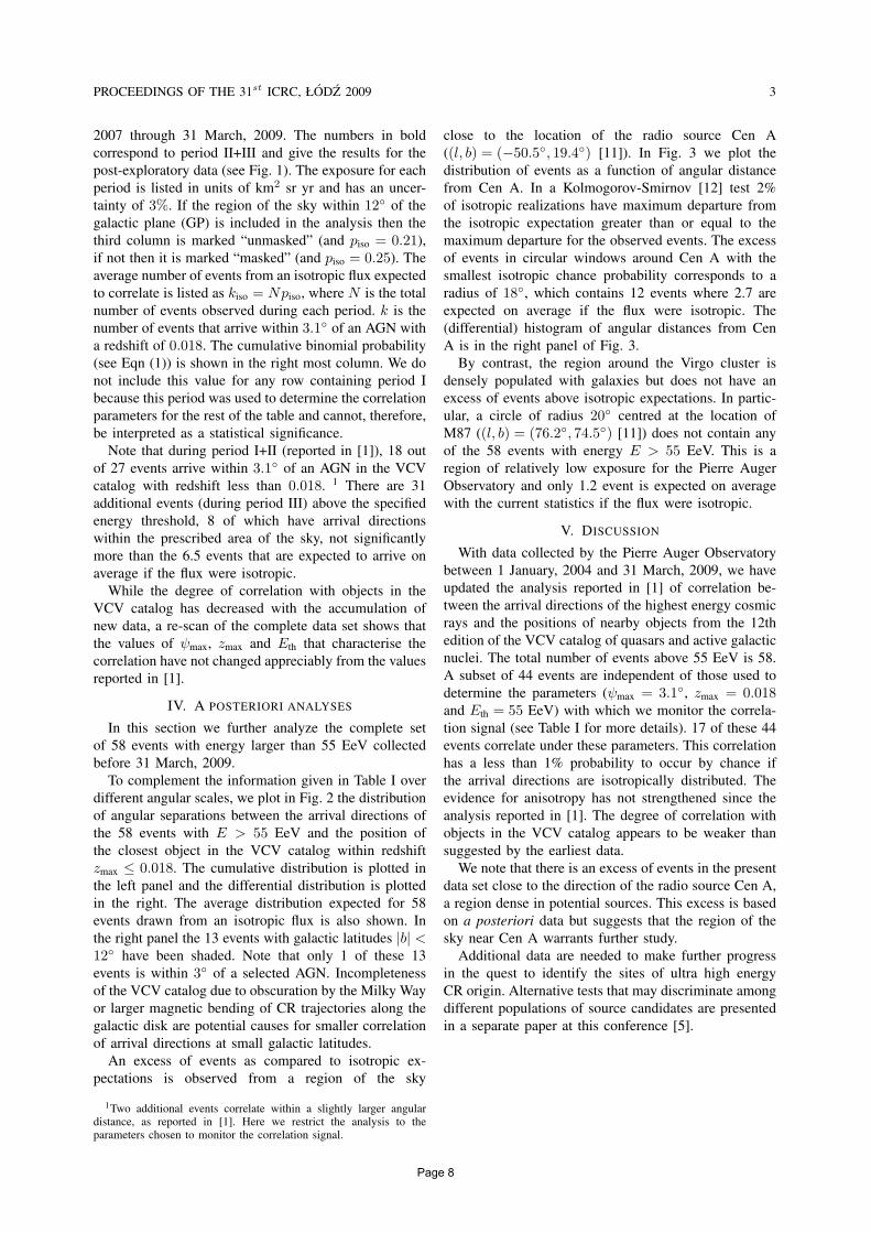
2007 through 31 March, 2009. The numbers in boldcorrespond to period II+III and give the results for thepost-exploratory data (see Fig. 1). The exposure for eachperiod is listed in units of km2 sr yr and has an uncer-tainty of 3%. If the region of the sky within 12 of thegalactic plane (GP) is included in the analysis then thethird column is marked “unmasked” (and piso = 0.21),if not then it is marked “masked” (and piso = 0.25). Theaverage number of events from an isotropic flux expectedto correlate is listed as kiso = Npiso, where N is the totalnumber of events observed during each period. k is thenumber of events that arrive within 3.1 of an AGN witha redshift of 0.018. The cumulative binomial probability(see Eqn (1)) is shown in the right most column. We donot include this value for any row containing period Ibecause this period was used to determine the correlationparameters for the rest of the table and cannot, therefore,be interpreted as a statistical significance.
Note that during period I+II (reported in [1]), 18 outof 27 events arrive within 3.1 of an AGN in the VCVcatalog with redshift less than 0.018. 1 There are 31additional events (during period III) above the specifiedenergy threshold, 8 of which have arrival directionswithin the prescribed area of the sky, not significantlymore than the 6.5 events that are expected to arrive onaverage if the flux were isotropic.
While the degree of correlation with objects in theVCV catalog has decreased with the accumulation ofnew data, a re-scan of the complete data set shows thatthe values of ψmax, zmax and Eth that characterise thecorrelation have not changed appreciably from the valuesreported in [1].
IV. A POSTERIORI ANALYSES
In this section we further analyze the complete setof 58 events with energy larger than 55 EeV collectedbefore 31 March, 2009.
To complement the information given in Table I overdifferent angular scales, we plot in Fig. 2 the distributionof angular separations between the arrival directions ofthe 58 events with E > 55 EeV and the position ofthe closest object in the VCV catalog within redshiftzmax ≤ 0.018. The cumulative distribution is plotted inthe left panel and the differential distribution is plottedin the right. The average distribution expected for 58events drawn from an isotropic flux is also shown. Inthe right panel the 13 events with galactic latitudes |b| <12 have been shaded. Note that only 1 of these 13events is within 3 of a selected AGN. Incompletenessof the VCV catalog due to obscuration by the Milky Wayor larger magnetic bending of CR trajectories along thegalactic disk are potential causes for smaller correlationof arrival directions at small galactic latitudes.
An excess of events as compared to isotropic ex-pectations is observed from a region of the sky
1Two additional events correlate within a slightly larger angulardistance, as reported in [1]. Here we restrict the analysis to theparameters chosen to monitor the correlation signal.
close to the location of the radio source Cen A((l, b) = (−50.5, 19.4) [11]). In Fig. 3 we plot thedistribution of events as a function of angular distancefrom Cen A. In a Kolmogorov-Smirnov [12] test 2%of isotropic realizations have maximum departure fromthe isotropic expectation greater than or equal to themaximum departure for the observed events. The excessof events in circular windows around Cen A with thesmallest isotropic chance probability corresponds to aradius of 18, which contains 12 events where 2.7 areexpected on average if the flux were isotropic. The(differential) histogram of angular distances from CenA is in the right panel of Fig. 3.
By contrast, the region around the Virgo cluster isdensely populated with galaxies but does not have anexcess of events above isotropic expectations. In partic-ular, a circle of radius 20 centred at the location ofM87 ((l, b) = (76.2, 74.5) [11]) does not contain anyof the 58 events with energy E > 55 EeV. This is aregion of relatively low exposure for the Pierre AugerObservatory and only 1.2 event is expected on averagewith the current statistics if the flux were isotropic.
V. DISCUSSION
With data collected by the Pierre Auger Observatorybetween 1 January, 2004 and 31 March, 2009, we haveupdated the analysis reported in [1] of correlation be-tween the arrival directions of the highest energy cosmicrays and the positions of nearby objects from the 12thedition of the VCV catalog of quasars and active galacticnuclei. The total number of events above 55 EeV is 58.A subset of 44 events are independent of those used todetermine the parameters (ψmax = 3.1, zmax = 0.018and Eth = 55 EeV) with which we monitor the correla-tion signal (see Table I for more details). 17 of these 44events correlate under these parameters. This correlationhas a less than 1% probability to occur by chance ifthe arrival directions are isotropically distributed. Theevidence for anisotropy has not strengthened since theanalysis reported in [1]. The degree of correlation withobjects in the VCV catalog appears to be weaker thansuggested by the earliest data.
We note that there is an excess of events in the presentdata set close to the direction of the radio source Cen A,a region dense in potential sources. This excess is basedon a posteriori data but suggests that the region of thesky near Cen A warrants further study.
Additional data are needed to make further progressin the quest to identify the sites of ultra high energyCR origin. Alternative tests that may discriminate amongdifferent populations of source candidates are presentedin a separate paper at this conference [5].
Page 8

4 HAGUE et al. CORRELATION OF COSMIC RAYS WITH EXTRAGALACTIC OBJECTS
Angular distance (degrees)0 5 10 15 20 25 30
Eve
nts
0
10
20
30
40
50
Data
Isotropic
Angular distance (degrees)0 5 10 15 20 25 30
Eve
nts
0
10
20
30
40
50
Angular distance (degrees)0 5 10 15 20 25 30
Eve
nts
0
2
4
6
8
10
12Data
oData with |b|<12
Isotropic
Angular distance (degrees)0 5 10 15 20 25 30
Eve
nts
0
2
4
6
8
10
12
Fig. 2. The distribution of angular separations between the 58 events with E > 55 EeV and the closest AGN in the VCV catalog within75 Mpc. Left: The cumulative number of events as a function of angular distance. The 68% the confidence intervals for the isotropic expectationis shaded blue. Right: The histogram of events as a function of angular distance. The 13 events with galactic latitudes |b| < 12 are shownwith hatching. The average isotropic expectation is shaded brown.
Cen Aψ
0 20 40 60 80 100 120 140 160
Eve
nts
0
10
20
30
40
50
Cen Aψ
0 20 40 60 80 100 120 140 160
Eve
nts
0
10
20
30
40
50 Data
Isotropic
Cen Aψ
0 20 40 60 80 100 120 140 160
Eve
nts
0
1
2
3
4
5
6
Data
Isotropic
Cen Aψ
0 20 40 60 80 100 120 140 160
Eve
nts
0
1
2
3
4
5
6
Fig. 3. Left: The cumulative number of events with E ≥ 55 EeV as a function of angular distance from Cen A. The average isotropicexpectation with approximate 68% confidence intervals is shaded blue. Right: The histogram of events as a function of angular distance fromCen A. The average isotropic expectation is shaded brown.
REFERENCES
[1] The Pierre Auger Collaboration. Science, 318:938–943, 2007 andAstropart. Phys., 29:188–204, 2008.
[2] M.-P. Veron-Cetty and P. Veron. Astron. Astrophys., 455:773–777, 2006.
[3] The Pierre Auger Collaboration, Phys. Rev. Lett. 101:061101(2008).
[4] The HiRes Collaboration, Phys. Rev. Lett. 100:101101 (2008).[5] J. Aublin for the Pierre Auger Collaboration, “Discriminating
potential astrophysical sources of the highest energy cosmic rayswith the Pierre Auger Observatory”, Proceedings of the 31stICRC, Lodz, Poland, 2009.
[6] F. Schussler for the Pierre Auger Collaboration, “Measurementof the cosmic ray energy spectrum above 1018 eV with thePierre Auger Observatory,” Proceedings of the 31st ICRC, Lodz,Poland, 2009.
[7] C. Di Giulio for the Pierre Auger Collaboration, “Energy cal-ibration of data recorded with the surface detectors of thePierre Auger Observatory,” Proceedings of the 31st ICRC, Lodz,Poland, 2009.
[8] C. Bonifazi for the Pierre Auger Collaboration, “The angularresolution of the Pierre Auger Observatory,” Nuclear Physics B(Proc. Suppl.) 190 (2009) 20-25.
[9] A. Wald “Sequential Analysis”, John Wiley and Sons, New York,1947.
[10] S. Y. BenZvi et al. , The Astrophysical Journal, 687:1035–1042,2008.
[11] NASA/IPAC Extragalactic Database. http://nedwww.ipac.caltech.edu/.
[12] W. T. Eadie et al. Statistical Methods in Experimental Physics.North-Holland, Amsterdam, 1971. pp 269–271.
Page 9

1
Discriminating potential astrophysical sources of the highestenergy cosmic rays with the Pierre Auger Observatory
Julien Aublin∗, for the Pierre Auger Collaboration†
∗ LPNHE, Universite Paris 6, 4 place Jussieu, 75252 Paris Cedex 05, France†Pierre Auger Observatory, av. San Martın Norte 304, (5613) Malargue, Argentina.
Abstract. We compare the distribution of arrivaldirections of the highest energy cosmic rays detectedby the Pierre Auger Observatory from 1 January2004 to 31 March 2009 with that of populations of po-tential astrophysical sources. For this purpose, we useseveral complementary statistical tests allowing oneto describe and quantify the degree of compatibilitybetween data and a given catalogue of sources. Weapplied these tests to active galactic nuclei detectedin X-rays by SWIFT-BAT and to galaxies found inthe HI Parkes and in the 2 Micron All-Sky Surveys.
Keywords: UHECRs, Anisotropy, Astrophysicalcatalogues
I. I NTRODUCTION
The origin and nature of the ultra high energy cosmicrays (UHECRs) are still unknown after more than halfa century since their discovery. The deflections en-countered by UHECRs during their propagation throughgalactic and extra galactic magnetic fields make a directidentification of their sources difficult.
Recently, the Pierre Auger Collaboration reported acorrelation between the arrival directions of the highestenergy events observed (E ≥ 6 × 10¹⁹ eV) and thedirections of known active galaxies closer than 100Mpc [1], [2]. An update of this analysis [3] with datacollected up to 31 March 2009 shows that the evidencefor anisotropy remains at the 99% confidence level,although the correlation has not strenghtened. In anycase, this result does not imply that AGN are indeedthe actual sources of UHECRs, since many other sourcescenarios could in principle reproduce the observed data.
In the present study, we compare the arrival directionsof data from the Pierre Auger Observatory with theposition of potential astrophysical sources. First, wecompute the standard cross-correlation function betweenthe observed arrival directions and a volume-selectedsample of galaxies from the 2MRS [4] catalogue, underthe simple assumption of an equal contribution of eachsource to the cosmic ray flux. Then we compare our datawith three different catalogues (X-ray AGNs detected bySWIFT [5], galaxies in the HI-Parkes [6], [7] and 2MRSsurveys) taking into account the intrinsic luminosity andthe distance of the sources. For this comparison, we usetwo complementary methods: a likelihood test and a testbased on the scalar product of functions on the sphere.
II. DATA SET
The data set consists of 58 events recorded by thePierre Auger Observatory from 1 January 2004 to 31March 2009, with energies reconstructed above55 EeVand zenith angles smaller than60. The energy resolu-tion is 17% , with a systematic uncertainty of22%[8].The angular resolution, defined as the angular radiusthat would contain68% of the reconstructed events is≤ 0.9. We use the energy threshold that maximizesthe departure from isotropy through the correlation withAGN [1]. This particular value corresponds to the regionwhere the energy spectrum of UHECRs [8] presents asignificant deviation from the power-law extrapolatedfrom lower energy. This supports the idea of a sharpreduction of the cosmic rays horizon due to the GZKeffect [9], [10], at energies greater than≃ 50− 60 EeV,limiting drastically the number of contributing sources.
III. A STROPHYSICAL CATALOGUES
Recent analysis comparing Auger data with theSWIFT-BAT and HIPASS catalogues can be found in[11], [12], [13]. The 22 months SWIFT-BAT [5] cat-alogue provides the most uniform all-sky hard X-raysurvey to date, it contains a total of 261 Seyfert galax-ies and AGN. The HIPASS [6], [7] galaxy cataloguecontains a large number of extragalactic HI sources thatcould host preferentially GRBs and magnetars producingUHECRs. Here, we adopt the flux limitSint > 9.4 Jykm s−1 following [13], leading to a total number of3058 galaxies. As in [12], we also consider a sub-sampleof the HIPASS catalogue, that we call HIPASS HL inthe following text, that contains the 765 most luminousgalaxies. We use the compilation (2MRS) provided byHuchra et al. [4] of the redshifts of theKmag < 11.25brightest galaxies from the 2MASS[14] catalogue. Thecatalogue, containing≃ 23000 sources, provides anexcellent image of the distribution of local matter. Forthe cross-correlation analysis, we use a volume-selectedsample of galaxies from the 2MRS catalogue (2MRSVS thereafter) to prevent a bias toward the faint galaxiesat small distances. We select galaxies with10 Mpc <
d < 200 Mpc and absolute magnitudesMk < −25.25,leading to 1940 objects in this sub-sample. For 2MRS,we exclude from the analysis UHECRs events (andsources for 2MRS VS) that have|b| < 10 to avoid abias due to incompleteness in the galactic plane region.
Page 10
2
IV. DATA ANALYSIS
A. Cross-correlation
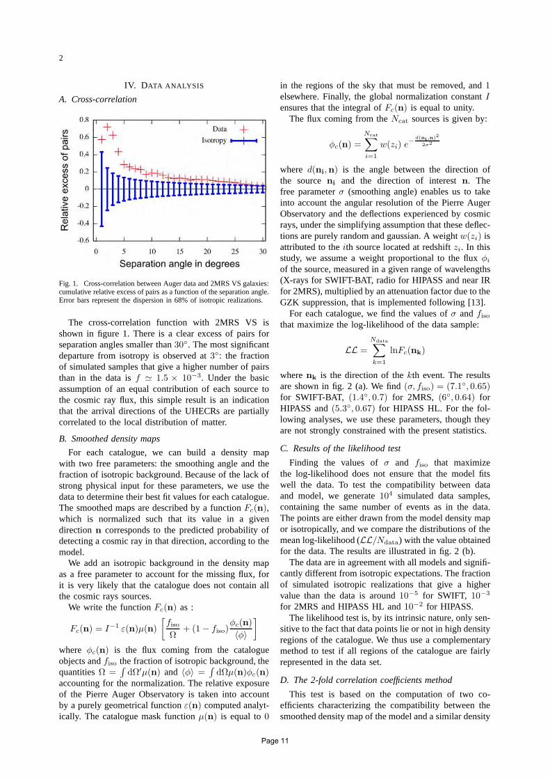
Fig. 1. Cross-correlation between Auger data and 2MRS VS galaxies:cumulative relative excess of pairs as a function of the separation angle.Error bars represent the dispersion in 68% of isotropic realizations.
The cross-correlation function with 2MRS VS isshown in figure 1. There is a clear excess of pairs forseparation angles smaller than30. The most significantdeparture from isotropy is observed at3: the fractionof simulated samples that give a higher number of pairsthan in the data isf ≃ 1.5 × 10⁻³. Under the basicassumption of an equal contribution of each source tothe cosmic ray flux, this simple result is an indicationthat the arrival directions of the UHECRs are partiallycorrelated to the local distribution of matter.
B. Smoothed density maps
For each catalogue, we can build a density mapwith two free parameters: the smoothing angle and thefraction of isotropic background. Because of the lack ofstrong physical input for these parameters, we use thedata to determine their best fit values for each catalogue.The smoothed maps are described by a functionFc(n),which is normalized such that its value in a givendirection n corresponds to the predicted probability ofdetecting a cosmic ray in that direction, according to themodel.
We add an isotropic background in the density mapas a free parameter to account for the missing flux, forit is very likely that the catalogue does not contain allthe cosmic rays sources.
We write the functionFc(n) as :
Fc(n) = I−1 ε(n)µ(n)
[fiso
Ω+ (1 − fiso)
φc(n)
〈φ〉
]
where φc(n) is the flux coming from the catalogueobjects andfiso the fraction of isotropic background, thequantitiesΩ =
∫dΩ′µ(n) and 〈φ〉 =
∫dΩµ(n)φc(n)
accounting for the normalization. The relative exposureof the Pierre Auger Observatory is taken into accountby a purely geometrical functionε(n) computed analyt-ically. The catalogue mask functionµ(n) is equal to0
in the regions of the sky that must be removed, and1elsewhere. Finally, the global normalization constantI
ensures that the integral ofFc(n) is equal to unity.The flux coming from theNcat sources is given by:
φc(n) =
Ncat∑
i=1
w(zi) e−
d(ni,n)2
2σ2
where d(ni,n) is the angle between the direction ofthe sourceni and the direction of interestn. Thefree parameterσ (smoothing angle) enables us to takeinto account the angular resolution of the Pierre AugerObservatory and the deflections experienced by cosmicrays, under the simplifying assumption that these deflec-tions are purely random and gaussian. A weightw(zi) isattributed to theith source located at redshiftzi. In thisstudy, we assume a weight proportional to the fluxφi
of the source, measured in a given range of wavelengths(X-rays for SWIFT-BAT, radio for HIPASS and near IRfor 2MRS), multiplied by an attenuation factor due to theGZK suppression, that is implemented following [13].
For each catalogue, we find the values ofσ andfiso
that maximize the log-likelihood of the data sample:
LL =
Ndata∑
k=1
lnFc(nk)
wherenk is the direction of thekth event. The resultsare shown in fig. 2 (a). We find(σ, fiso) = (7.1, 0.65)for SWIFT-BAT, (1.4, 0.7) for 2MRS, (6, 0.64) forHIPASS and(5.3, 0.67) for HIPASS HL. For the fol-lowing analyses, we use these parameters, though theyare not strongly constrained with the present statistics.
C. Results of the likelihood test
Finding the values ofσ and fiso that maximizethe log-likelihood does not ensure that the model fitswell the data. To test the compatibility between dataand model, we generate104 simulated data samples,containing the same number of events as in the data.The points are either drawn from the model density mapor isotropically, and we compare the distributions of themean log-likelihood (LL/Ndata) with the value obtainedfor the data. The results are illustrated in fig. 2 (b).
The data are in agreement with all models and signifi-cantly different from isotropic expectations. The fractionof simulated isotropic realizations that give a highervalue than the data is around10−5 for SWIFT, 10−3
for 2MRS and HIPASS HL and10−2 for HIPASS.The likelihood test is, by its intrinsic nature, only sen-
sitive to the fact that data points lie or not in high densityregions of the catalogue. We thus use a complementarymethod to test if all regions of the catalogue are fairlyrepresented in the data set.
D. The 2-fold correlation coefficients method
This test is based on the computation of two co-efficients characterizing the compatibility between thesmoothed density map of the model and a similar density
Page 11

3
(a) (b)
Fig. 2. (a) Probability contours for the log-likelihood maximisation. The maximum is indicated by a black point. (b) Distributions of meanlog-likelihood per event for the isotropy (labelled as I) and for the model (II). Data is indicated by a black vertical line.
map computed for the data. We apply a gaussian filteringto theNdata data points to obtain the following densitymap:
Fd(n) =µ(n)
2πσ2 Ndata
Ndata∑
j=1
exp
(−
d(nj,n)2
2σ2
)
The first coefficient, called ”correlation coefficient” isgiven by:
C(Fd, Fc) =
∫Fc(n)Fd(n) dΩ√∫ (
Fc(n))2
dΩ∫ (
Fd(n))2
dΩ
This coefficient ranges from 0 (Fc and Fd are an-ticorrelated) to 1 (Fc and Fd are identical). A highvalue ofC(Fd, Fc) indicates a good match between dataand model distributions. The second coefficient, called”concentration coefficient” is defined by:
Idd =
∫F 2
d (n) dΩ.
This second observable carries the information about theintrinsic clustering properties of the angular distributionof the data. The magnitude ofIdd depends on the densitymap contrast: it is maximum if all the data points havethe same position on the sky, and minimum if thepoints are uniformly distributed on the sphere. Thesecoefficients are related to the standard two point crossand auto-correlation functions.
For each model, we generate104 simulated samplescontaining the same number of events as in the data.The points are either drawn from the model density mapor isotropically. Fulfilling the test requires that bothCandIdd distributions obtained with simulated sample arecompatible with the values computed with the data.
The results of the test are shown in fig. 3. Thedata are compatible with all models, the map basedon SWIFT-BAT gives, as in the likelihood test, themost discriminant test against isotropy. The fraction ofisotropic simulations that have both a higher correlationand concentration coefficients than the data is∼ 4×10⁻³
for HIPASS and lower than10−4 for SWIFT-BAT.
V. CONCLUSION
The Pierre Auger Observatory has recorded 58 cosmicrays with energiesE > 55 EeV between 1 January 2004and 31 March 2009. Different complementary tests areapplied to extract information about the compatibilitybetween the arrival directions of Auger events andmodels based on catalogues of potential astrophysicalsources or isotropic distributions.
When performing a cross-correlation analysis with the2MRS VS catalogue, we find an excess of pairs overa range of angular scales, indicating that the UHECRsmay be partially correlated to the distribution of localmatter (under a basic ”equal flux” assumption). We thenapply two other tests that require the computation ofsmoothed maps of expected cosmic ray flux. The mapshave two free parameters, that are determined throughthe maximization of the likelihood of the data.
The log-likelihood and the 2-fold correlation coef-ficients tests show that our data are different fromisotropic expectations and compatible with the modelsbased on SWIFT-BAT, 2MRS and HIPASS catalogueswith the parameters maximizing the likelihood. Withinone standard deviation, these parameters areσ ≤ 10
and fiso ∈ [0.4; 0.8]. The map based on SWIFT-BATgives the most discriminant test against isotropy.
Page 12

4
(a) SWIFT-BAT (b) 2MRS
(c) HIPASS (d) HIPASS High Luminosity
Fig. 3. Two dimensional distributions of the correlation and concentration coefficient for isotropic simulations (labelled as I) and for the model(labelled as II). The value obtained with data is indicated by a black point. The individual distributions of the correlation and concentrationcoefficients are shown, the data being indicated by a vertical line.
REFERENCES
[1] Pierre Auger Collaboration.Science, 318:939, 2007.
[2] Pierre Auger Collaboration.Astroparticle Physics, 29:188, 2008.
[3] J.D. Hague for the Pierre Auger Collaboration.Proceedings ofthe 31st ICRC, 2009.
[4] J. Huchra et al.IAU Symposium, No. 216, 170, 2005.
[5] J. Tueller et al.[arXiv:0903.3037], 2009.
[6] M. J. Meyer et al.MNRAS, 350:1195, 2004.
[7] O.I Wong et al.MNRAS, 371:1855, 2006.[8] C. Di Giulio for the Pierre Auger Collaboration.Proceedings of
the 31st ICRC, 2009.[9] K. Greisen. Phys. Rev. Lett., 16:748, 1966.
[10] G. T. Zatsepin and V.A. Kuzmin.JETP Lett., 4:78, 1966.[11] M. R. George et al.MNRAS, 388:773, 2008.[12] G. Ghisellini et al.MNRAS, 390:L88–L92, 2008.[13] D. Harari, S. Mollerach and E. Roulet.MNRAS, 394:916–922,
2009.[14] T. H. Jarrett, T. Chester, R. Cutri, S. Schneider, M. Skrutskie,
and J. P. Huchra.Astronom. J., 119:2498–2531, 2000.
Page 13

PROCEEDINGS OF THE 31st ICRC, ŁODZ 2009 1
Search for intrinsic anisotropy in the UHECRs data from thePierre Auger Observatory
J. R. T. de Mello Neto∗, for the Pierre Auger Collaboration†
∗Instituto de Fısica, Universidade Federal do Rio de Janeiro, Ilha do Fundao, Rio de Janeiro, Brazil† Pierre Auger Observatory, Av. San Martın Norte 304, (5613) Malargue, Argentina
Abstract. We discuss techniques which have beendeveloped for determining the intrinsic anisotropyof sparse ultra-high-energy cosmic ray datasets, in-cluding a two point, an improved two point anda three point method. Monte-Carlo studies of thesensitivities of these tests are presented. We performa scan in energy above the 100 highest energy events(corresponding to ≃43 EeV) detected at the PierreAuger Observatory and find that the largest deviationfrom isotropic expectations occurs for events above52 EeV.
Keywords: UHECRs, anisotropy, autocorrelation
I. I NTRODUCTION
The origin of ultra-high energy cosmic rays (UHE-CRs) with energies greater then1018 eV has been alongstanding mystery since their discovery about 50years ago [1]. The Pierre Auger Collaboration has re-cently shown that the flux of cosmic rays is stronglysuppressed above4 × 1019 eV [2], providing evidencefor the 1966 prediction of Greisen [3] and of Zatsepinand Kuz’min [4] (GZK). The effect of energy lossescombined with the anisotropic distribution of matter inthe 100 Mpc volume around us suggests that cosmicrays at the highest energies are likely to be distributedanisotropically. This expectation of anisotropy above theGZK threshold was verified in 2007 [5], [6], when theAuger Collaboration reported an evidence for anisotropyat a C.L. of at least 99% using the correlation of thecosmic rays detected at the Pierre Auger Observatorywith energies above∼ 6 × 10¹⁹ eV and the positionsof the galaxies in the Veron-Cetty & Veron [7] (VCV)catalogue of active galactic nuclei (AGNs).
Here we report on tests designed to answer thequestion of whether the arrival directions of the highest-energy events observed by Auger are consistent withbeing drawn from an isotropic distribution, with no ref-erence to an association with AGN or other extragalacticobjects. The goal is to test for anisotropy using only thecosmic-ray data.
II. STATISTICAL METHODS
At the highest energies, the steepening of the energyspectrum makes the current statistics so small that ameasure of a statistically significant departure fromisotropy is hard to establish, especially when using blindgeneric tests. This motivated us to test several methodsby challenging their power for detecting anisotropy using
simulated samples with few data points (typically lessthan 100) drawn from different kinds of anisotropiesboth in large and small scales. We report in this paper onauto-correlation analyses, using differential approachesbased on a 2pt function, an extended 2pt function(refered to as 2pt+ in the following), and a 3pt function.
The standard 2pt function [8] was used as a reference.We histogrammed the number of event pairs within agiven angular distance in bins of 5 and compared it tothe isotropic expectation obtained from a large number(typically 106) of Monte-Carlo samples. The departurefrom isotropy is then measured through a pseudo-log-likelihood ΣP :
ΣdataP =
N∑
i=1
lnP(niobs|n
iexp),
where niobs and ni
exp are the observed and expectednumber of event pairs in bini and P the Poissondistribution. The resultingΣdata
P is then compared to thedistribution ofΣP obtained from isotropic Monte-Carlosamples. The probabilityP for the data to come fromthe realisation of an isotropic distribution is calculatedas the fraction of samples havingΣP lower thanΣdata
P .A statistics was constructed to add the orientation
information of the event pairs to the 2pt information[9].The new estimator, 2pt+, is calculated on the data andon a large set of Monte-Carlo samples in the same waythan in the 2pt case. Again, the departure from isotropyis measured by the fraction of samples giving a 2pt+estimate smaller than the data.
Finally, we also constructed a 3pt method basedon [10] where, for each triangle defined by a tripletof data points, a shape (round or elongated) and astrength (small or big) parameter can be calculated. The2 dimensional distribution of these parameters from thedata is then compared to the average expectation froma large set of Monte-Carlo samples of the same size bymeans of the same log-likelihood method with Poissonstatistics than in the previous cases. More details can befound in [11].
III. M ONTE-CARLO STUDIES
A test is usually defined in terms of athresholdα,which is the probability against the wrong rejectionof the null hypothesis (in our case wrongly rejectingisotropy or claiming an anisotropy while there is not),and of a power 1 − β, which is the probability to
Page 14

2 DE MELLO NETO et al. SEARCH FOR INTRINSIC ANISOTROPY
Number of Events
20 40 60
)β P
ower
(1-
-110
1
2pt2pt+3pt
Number of Events
20 40 60 80 100
)β P
ower
(1-
-210
-110
1 2pt2pt+3pt
Fig. 1. Power of the 2pt (filled circles), 2pt+ (filled squares)and 3pt (empty circles) tests as a function of the number ofevents, for 2 threshold values: 1% (lines) and 0.1% (dottedlines). Events are drawn from nearby (z ≤ 0.018) AGNfrom [7] with no isotropic background (upper panel) and 50%isotropic background (lower panel).
successfully claim anisotropy when it exits. A good testis a test that for a given number of events and a giventhresholdα has a high power1 − β. When the powerof a test is less than 90%, the test may often miss atrue signal. In this section, we present the power of thethree tests at different thresholdsα as a function of thenumber of events, based on mock samples inspired fromthe correlation of UHECRs with nearby extragalacticobjects we reported in [5], [6].
We first built fair samples of the VCV catalogueof AGNs with redshiftz ≤ 0.018, accounting for theexposure function of the experiment. On the upper panelof Fig.1, we show the power of the 2pt test (filledcircles), of the 2pt+ test (filled squares) and of the3pt test (empty circles) as a function of the number ofevents. Two thresholds are illustrated:α = 1% (lines)and α = 0.1% (dotted lines). Whatever the number ofevents, the 2pt+ and 3pt tests are always more powerfulthan the standard 2pt one, and this is even more the casewhen the number of events decreases. Meanwhile, below50 events, the power of each test is rapidly getting lowereven in the case of a 1% threshold, reaching only lessthan 50% at best with 20 events.
minE
40 50 60 70 80
P
-310
-210
-110
1
2pt+3pt
Fig. 2. Significance of the anisotropy in the highest energyevents as a function ofEmin. Filled squares (empty circles)are the probability values calculated using the 2pt+ method(3pt method). The largest departure from isotropy is found atenergy of about 52 EeV.
We show the same analysis on the lower panel of Fig.1but by adding a 50% mixture of isotropic events to theanisotropic signal. All tests are then less sensitive thanin the previous case, the power of the best of them (3pt)being always below 90% even with a threshold of 1%,and reaching only few % when dealing with 20 events.
It thus turns out that at low statistics, the sensitivity ofthe tests gets rapidly diluted, their power never reaching90% unless a strong signal of anisotropy is present inthe data set.
IV. A PPLICATION TO THE DATA
The data set we use in this analysis consists of the100 highest energy events (corresponding to energiesgreater than≃43 EeV) with zenith angles smaller than60 recorded by the surface detector of the Pierre AugerObservatory from January, 1st 2004 to March, 31st
2009. The energy resolution is 17%, with a systematicuncertainty fo 22% [2]. The angular resolution, definedas the angular radius around the true cosmic ray directionthat would contain 68% of the reconstructed showerdirections, is at these energies better than0.9[13]. Thefiducial cut implemented in the present analysis requiresthat at least 5 active nearest detectors surround the onewith the highest signal when the event was recorded,and that the reconstructed shower core is inside an activeequilateral triangle of detectors.
Applying both 2pt+ and 3pt estimators, we performeda scan in energy to search for intrinsic anisotropy. Weshow in Fig.2 the results of this scan, starting fromthe 20 highest energy events (Emin ≃ 73 EeV), andlowering the energy threshold by adding each time the10 next events up to the 100 highest energy events(Emin ≃ 43 EeV). The filled squares are the resultsobtained using the 2pt+ method, while the empty circlesare the results obtained using the 3pt method. Themaximal departure from isotropy is observed to occur at≃ 52 EeV (for the 70 highest energy events) using both
Page 15

PROCEEDINGS OF THE 31st ICRC, ŁODZ 2009 3
methods: at this energy threshold, the probabilityP forthe data to be a realisation of an isotropic backgroundis P = 0.26% using the 2pt+ estimator andP = 0.56%using the 3pt estimator. For higher energy thresholds,both methods give results above the % level. As expectedfrom the second toy model described in the previoussection, the relatively low power of the tests whenlowering the number of events prevents us to concludeon the isotropic or anisotropic nature of the sky fromthese observations.
The numbers reported here do not take into accountthe penalties associated to the scan in energy. In anycase, as all those analyses were performeda posteriori,this prevents us to rigorously report on probabilities thatcould be taken at face value.
In Fig.3, we illustrate the largest departure fromisotropy we found in the data using the 3pt method, byshowing the log-likelihood of individual bins in shape-strength parameter space of data above 52 EeV comparedagainst isotropic expectations (upper panel). Because ofbin-bin correlations, the method sums the log-likelihoodsto obtain Σdata
P and compares them against isotropicskies to determine the probability that an isotropicdistribution may produce this pattern at random. Thedistribution ofΣP for 2× 10⁴ isotropic skies is plottedwith black hatching in the lower panel. As in the 2ptand the 2pt+ cases, the departure from isotropy is thenobtained by counting the number of isotropic Monte-Carlo skies with a lowerΣP than the one observed inthe data.
V. CONCLUSION
We have reported three statistical methods to searchfor intrinsic anisotropy of the UHECRs data measured atthe Pierre Auger Observatory. Despite of the sensitivityimprovement that the 2pt+ and 3pt tests bring withrespect to the standard 2pt test, they still show relativelylow power at low statistics, as estimated on toy Monte-Carlo samples drawn with the help of catalogues ofnearby astronomical objects. This makes difficult thedetection of anisotropy independently of any catalogueof astronomical objects even at 99% confidence levelwith the current statistics we are dealing with at thehighest energies. On the contrary, tests designed oncorrelation of UHECRs with the positions of nearbyastronomical objects are more powerful to provide evi-dence for anisotropy [14], [15]. More statistics is clearlynecessary to establish any anisotropy claim using thekind of blind generic tests we presented in this paper.
Fig. 3. Top: for each bin in shape and strength, we plot thenatural-log of the Poisson probability to observenobs tripletsgiven nexp expected from an isotropic sky, in shades of blue.Bottom : The distribution ofΣP for 2× 10
4 isotropic skies isplotted with black hatching. The significance is calculatedbycounting the number of isotropic Monte-Carlo skies to the leftof the data (dashed red line).
REFERENCES
[1] Nagano M. and Watson A. A., Rev. Mod. Phys. 72 (2000) 689.[2] [Pierre Auger Collaboration], Phys. Rev. Lett.101, 061101
(2008)[3] Greisen, K., Phys. Rev. Lett., 16 (1966) 748.[4] Zatsepin, G. T., & Kuzmin, V. A., PisIma Zh. Eksp. Teor. Fiz.,
4 (1966) 114.[5] [Pierre Auger Collaboration], Science318, 938 (2007)[6] [Pierre Auger Collaboration], Astropart. Phys.29, 188 (2008)
[Erratum-ibid.30, 45 (2008)][7] M.-P. Veron-Cetty and P. Veron, Astron. & Astrophys. 455(2006)
773.[8] The Large-Scale Structure of the Universe, Princeton University
Press, (1980).[9] M. Ave et al., submited to JCAP.
[10] Fisher, N.I. and T. Lewis and B.J.J. Embleton,Statistical Analysisof Spherical Data, Cambridge University Press, (1987).
[11] J. D. Hagueet al., submited to Journal of Physics G.[12] [Pierre Auger Collaboration], Nucl. Instrum. Meth. A586, 409
(2008)[13] C. Bonifazi [Pierre Auger Collaboration], Nuclear Physics B
(Proc. Suppl.) 190 (2009) 20-25 arXiv:0901.3138 [astroph-HE][14] J. D. Hague for The Pierre Auger Collaboration, Proceedings of
the 31st ICRC, Lodz, Poland, 2009.[15] J.Aublin for The Pierre Auger Collaboration, Proceedings of the
31st ICRC, Lodz, Poland, 2009.
Page 16

PROCEEDINGS OF THE 31st ICRC, ŁODZ 2009 1
Ultra-high energy photon studies with the Pierre AugerObservatory
Piotr Homola∗ for the Pierre Auger Collaboration†
∗H. Niewodniczanski Institute of Nuclear Physics PAN, Radzikowskiego 152, 31-342 Krakow, Poland†Av. San Martin Norte 304 (5613) Malargue, Prov. de Mendoza, Argentina
Abstract. While the most likely candidates forcosmic rays above 1018 eV are protons and nuclei,many of the scenarios of cosmic ray origin predictin addition a photon component. Detection of thiscomponent is not only of importance for cosmic-rayphysics but would also open a new research windowwith impact on astrophysics, cosmology, particle andfundamental physics. The Pierre Auger Observatorycan be used for photon searches of unprecedentedsensitivity. At this conference, the status of this searchwill be reported. In particular the first experimentallimits at EeV energies will be presented.
Keywords: UHE photons, upper limits, Auger
I. INTRODUCTION
The composition of ultra-high energy cosmic rays(UHECR), i.e. those above 1018 eV, is still unknown.The Pierre Auger Observatory [1], the newly completedgiant air shower detector, with its unprecedented eventstatistics, brings us closer than ever to resolving thisissue. One of the theoretical candidates for UHECR arephotons. The first photon searches based on Auger dataresulted in upper limits on photon fractions and fluxes[2], [3]. So far, no primary CR photons were identified,the most significant upper limit on the photon fractionis 2% for photons of energies above 10 EeV, basedon the data collected by the surface array of particlecounters of the Pierre Auger Observatory. This limitseverely constrains the family of ’top-down’ models [4]which predict large photon contributions (up to 50%)to the observed CR flux. A smaller contribution withtypical values around ∼0.1% is expected in ’bottom-up’ models. Here, so-called ’GZK-photons’ originateduring the propagation of charged particles by photo-pion production with background radiation.
Until now, all UHE photon limits were placed at ener-gies larger than 10 EeV. In this work the first limits forphotons of energies down to 2 EeV are presented, basedon the data collected by the Pierre Auger Observatory.
II. DATA SET AND SELECTION CUTS
The Pierre Auger Observatory collects data withtwo independent techniques: a surface array of waterCherenkov detectors (Surface Detector - SD) and a net-work of fluorescence telescopes (Fluorescence Detector- FD). The analysis presented in this work concernsthe hybrid data (i.e. events recorded by both detectors)collected between December 2004 and December 2007.
Fig. 1. Relative exposure to primary photons, protons and iron nuclei,normalized to protons at 10 EeV, after applying the quality and fiducialvolume cuts with the requirement of the hybrid trigger (see text). Inorder to guide the eye polynomial fits are superimposed to the obtainedvalues.
The hybrid data statistics are reduced comparing to thepure SD data because of the limited FD duty cycle(∼13% of the total time). On the other hand, the ad-vantage of the hybrid technique is the direct observationof the longitudinal shower profile, reaching also to lowerenergies.
The requirements for the hybrid event selection in-clude a good quality of shower longitudinal profiles(e.g. enough FD phototubes triggered, good quality ofthe profile fit, small contamination of direct Cherenkovlight) and the shower maximum Xmax within the FDfield of view (see Ref. [5] and references therein). Ithas been proven before [2] that Xmax is a powerfuldiscriminating variable for photon searches (photon-induced showers in general reach their maxima deeperin the atmosphere than showers initiated by nuclei) andwe make use of this fact here.
To avoid biases introduced by the above requirementsa set of energy dependent fiducial volume cuts wasintroduced: nearly vertical showers and those landingtoo far from the detector were rejected from the analysis.Technical details and a complete list of the data selectioncuts with explanations can be found in Ref. [5].
After applying the selection criteria the acceptancesfor photon and nuclear primaries are similar in theenergy region of interest. This is shown in Fig. 1.The presented shower simulations were performed withCORSIKA [6] using QGSJET01 [7] and FLUKA [8]interaction models and processed through a complete
Page 17

2 P. HOMOLA et al. UHE PHOTONS IN THE PIERRE AUGER OBSERVATORY
detector simulation and reconstruction chain [9]. Theapplication of all the cuts resulted in a data sampleof ntotal(Ethr) = 2063, 1021, 436 and 131 eventsabove the predefined energy thresholds: Ethr = 2, 3,5 and 10 EeV respectively. To account for the efficiencydependence on the primary energy, fiducial volumecut correction factors εfvc(Ethr) = 0.72, 0.77, 0.77and 0.77 were introduced for Ethr = 2, 3, 5 and 10EeV respectively. These corrections are conservative andindependent of the assumptions on the actual primaryfluxes (see Ref. [5] for details).
The presence of clouds during shower detection couldchange the efficiencies shown in Fig. 1. In particular, thereconstructed values of Xmax could be affected in casethe measured longitudinal profile is partially obscuredby clouds. In consequence, the primary particle couldbe misidentified. Thus, events are qualified as photoncandidates only when IR cloud cameras could verify theabsence of clouds. The fraction of events passing thiscloud cut was determined by individual inspection ofsubsets of the data sample to be εclc = 0.51.
III. THE PHOTON UPPER LIMITS AT EEV
To calculate the photon limit, the number of photoncandidates nγ has to be specified for all the consideredvalues of Ethr. This is done by constructing the photoncandidate cut as the median of the Xmax distributionfor photons. The relevant efficiency correction is thenεpcc = 0.5. The values of the median were extracted withdedicated simulations performed for primary photonswith geometry and energy corresponding to all thepotential photon candidates. A parametrization for thetypical median photon depth of shower maximum isshown as a solid line in Fig. 2, where the Xmax valuesare plotted versus the reconstructed event energies abovethe lowest considered threshold (2 EeV) for all the eventswith Xmax ≥ 800 g cm−2 after executing all the cutsdiscussed before. Statistical uncertainties are typically afew percent in energy and ∼ 15-30 g cm−2 in Xmax
while systematic uncertainties are ∼22% in energy and∼11 g cm−2 in Xmax. The photon candidates are locatedabove the pcc line in Fig 2: nγ−cand = 8, 1, 0, 0 for theconsidered threshold energies Ethr = 2, 3, 5 and 10EeV respectively. It has been checked that the observednumber of photon candidates is within the expectationsin case of nuclear primaries only. In Fig. 2 the 5% tailof the proton Xmax distribution is shown. We thereforeconclude that the observed photon candidate events maywell be due to nuclear primaries only.
With the candidate number and the efficiency correc-tions defined above, the 95% c.l. upper limit for photonfraction can be calculated as
F 95γ (Ethr) =
n95γ−cand(Ethr) 1
εfvc1
εpcc
ntotal(Ethr)εclc(1)
where n95γ−cand(Ethr) is the 95% c.l. upper limit on
the number of photon candidates. n95γ−cand(Ethr) was
Fig. 2. Measured depth of shower maximum vs. energy for deepXmax events (blue dots) after quality, fiducial volume and cloud cuts.Red crosses show the 8 photon candidate events (see text). The solidred line indicates the typical median depth of shower maximum forprimary photons.The dashed blue line indicates the 5% tail in theproton Xmax distribution using QGSJET 01.
calculated using the Poisson distribution and conserva-tively assuming no background of nuclear primaries. Theresultant 95% c.l. upper limits on the photon fractionsare 3.8%, 2.4%, 3.5% and 11.7% for the primary ener-gies above 2, 3, 5 and 10 EeV respectively.
The robustness of these results was checked againstdifferent sources of uncertainties. The variation of theselection criteria within the experimental resolution es-sentially does not affect the results. The effective to-tal uncertainty in Xmax for this analysis amounts to∼16 g cm−2 (see Ref. [5] for details). Increasing (re-ducing) all the reconstructed Xmax values by 16 g cm−2
increases (reduces) the number of photon candidatesonly for the two lowest energy thresholds: 2 and 3 EeV.The corresponding variations of the photon upper limitsare: F 95
γ (Ethr = 2 EeV) = 4.8% (3.8% – no variation)and F 95
γ (Ethr = 3 EeV) = 3.1% (1.5%).
IV. DISCUSSION
The current upper limits on photon fractions comparedto theoretical predictions are plotted in Fig. 3. The Augerhybrid photon upper limits above 2, 3, and 5 EeVplaced with this analysis are the first photon upperlimits below 10 EeV. The limit above 10 EeV is anupdate of the previous Auger hybrid limit published inRef. [2]. The predictions of ’top-down’ models weretested here in a new energy range and the constraintsfrom the Auger SD limits were confirmed by data takenwith the fluorescence technique. It should be noted thatthe presented limits together with the one published inRef. [2] are the only ones based on fluorescence data. Itis also worth mentioning that the previous 10 EeV SD
Page 18
PROCEEDINGS OF THE 31st ICRC, ŁODZ 2009 3
threshold energy [eV]
1910 2010
phot
on fr
actio
n
-410
-310
-210
-110
1
Auger South 20 years
threshold energy [eV]
1910 2010
phot
on fr
actio
n
-410
-310
-210
-110
1
SHDM
SHDM’
TD
Z Burst
GZKHP HP
A1
A1 A2
AY
Y
Y
Auger SD
Auger SD
Auger SD
Auger Hybrid
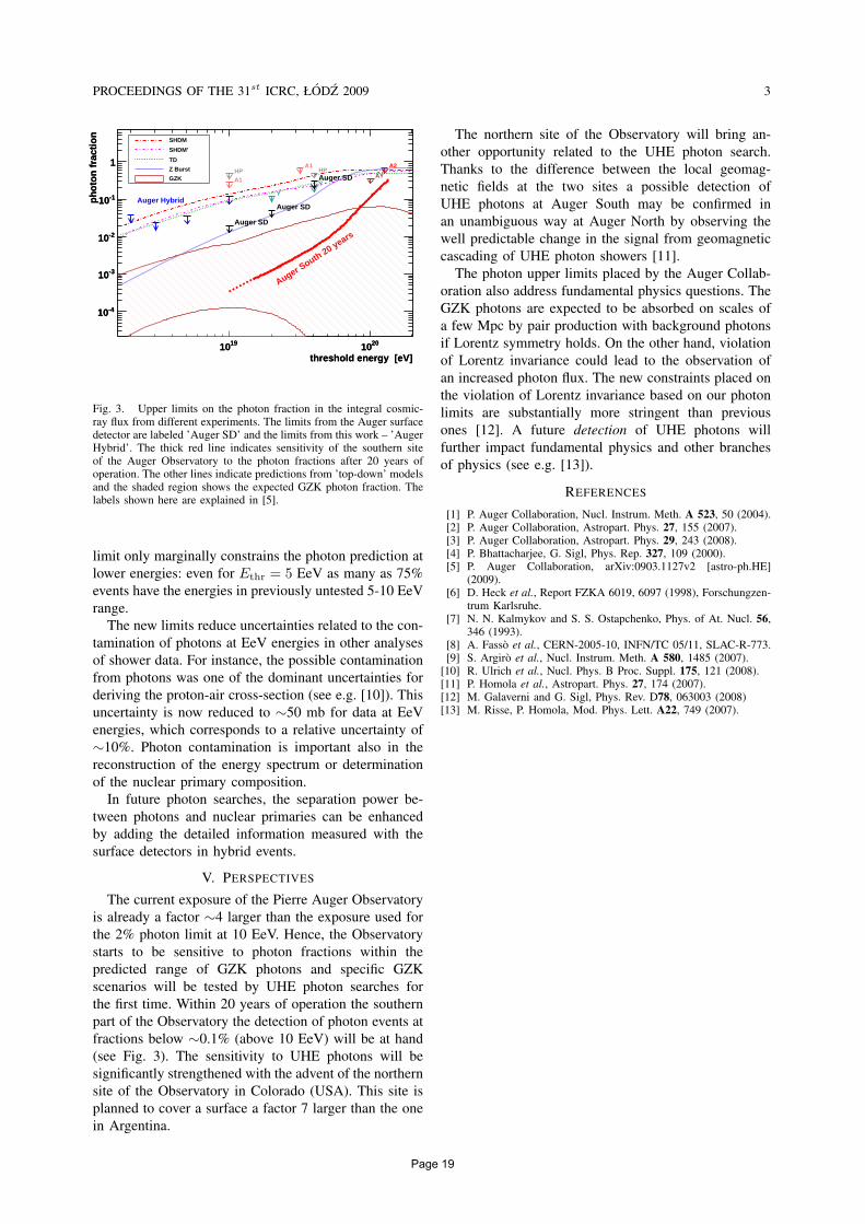
Fig. 3. Upper limits on the photon fraction in the integral cosmic-ray flux from different experiments. The limits from the Auger surfacedetector are labeled ’Auger SD’ and the limits from this work – ’AugerHybrid’. The thick red line indicates sensitivity of the southern siteof the Auger Observatory to the photon fractions after 20 years ofoperation. The other lines indicate predictions from ’top-down’ modelsand the shaded region shows the expected GZK photon fraction. Thelabels shown here are explained in [5].
limit only marginally constrains the photon prediction atlower energies: even for Ethr = 5 EeV as many as 75%events have the energies in previously untested 5-10 EeVrange.
The new limits reduce uncertainties related to the con-tamination of photons at EeV energies in other analysesof shower data. For instance, the possible contaminationfrom photons was one of the dominant uncertainties forderiving the proton-air cross-section (see e.g. [10]). Thisuncertainty is now reduced to ∼50 mb for data at EeVenergies, which corresponds to a relative uncertainty of∼10%. Photon contamination is important also in thereconstruction of the energy spectrum or determinationof the nuclear primary composition.
In future photon searches, the separation power be-tween photons and nuclear primaries can be enhancedby adding the detailed information measured with thesurface detectors in hybrid events.
V. PERSPECTIVES
The current exposure of the Pierre Auger Observatoryis already a factor ∼4 larger than the exposure used forthe 2% photon limit at 10 EeV. Hence, the Observatorystarts to be sensitive to photon fractions within thepredicted range of GZK photons and specific GZKscenarios will be tested by UHE photon searches forthe first time. Within 20 years of operation the southernpart of the Observatory the detection of photon events atfractions below ∼0.1% (above 10 EeV) will be at hand(see Fig. 3). The sensitivity to UHE photons will besignificantly strengthened with the advent of the northernsite of the Observatory in Colorado (USA). This site isplanned to cover a surface a factor 7 larger than the onein Argentina.
The northern site of the Observatory will bring an-other opportunity related to the UHE photon search.Thanks to the difference between the local geomag-netic fields at the two sites a possible detection ofUHE photons at Auger South may be confirmed inan unambiguous way at Auger North by observing thewell predictable change in the signal from geomagneticcascading of UHE photon showers [11].
The photon upper limits placed by the Auger Collab-oration also address fundamental physics questions. TheGZK photons are expected to be absorbed on scales ofa few Mpc by pair production with background photonsif Lorentz symmetry holds. On the other hand, violationof Lorentz invariance could lead to the observation ofan increased photon flux. The new constraints placed onthe violation of Lorentz invariance based on our photonlimits are substantially more stringent than previousones [12]. A future detection of UHE photons willfurther impact fundamental physics and other branchesof physics (see e.g. [13]).
REFERENCES
[1] P. Auger Collaboration, Nucl. Instrum. Meth. A 523, 50 (2004).[2] P. Auger Collaboration, Astropart. Phys. 27, 155 (2007).[3] P. Auger Collaboration, Astropart. Phys. 29, 243 (2008).[4] P. Bhattacharjee, G. Sigl, Phys. Rep. 327, 109 (2000).[5] P. Auger Collaboration, arXiv:0903.1127v2 [astro-ph.HE]
(2009).[6] D. Heck et al., Report FZKA 6019, 6097 (1998), Forschungzen-
trum Karlsruhe.[7] N. N. Kalmykov and S. S. Ostapchenko, Phys. of At. Nucl. 56,
346 (1993).[8] A. Fasso et al., CERN-2005-10, INFN/TC 05/11, SLAC-R-773.[9] S. Argiro et al., Nucl. Instrum. Meth. A 580, 1485 (2007).
[10] R. Ulrich et al., Nucl. Phys. B Proc. Suppl. 175, 121 (2008).[11] P. Homola et al., Astropart. Phys. 27, 174 (2007).[12] M. Galaverni and G. Sigl, Phys. Rev. D78, 063003 (2008)[13] M. Risse, P. Homola, Mod. Phys. Lett. A22, 749 (2007).
Page 19

PROCEEDINGS OF THE 31st ICRC, ŁODZ 2009 1
Limits on the diffuse flux of ultra high energy neutrinos set usingthe Pierre Auger Observatory
Javier Tiffenberg∗, for the Pierre Auger Collaboration†
∗Facultad de Ciencias Exactas y Naturales, Univ. de Buenos Aires, Buenos Aires, ARGENTINA†Av. San Martın Norte 304 (5613) Malargue, Prov. de Mendoza, ARGENTINA
Abstract. The array of water-Cherenkov detectorsof the Pierre Auger Observatory is sensitive toneutrinos of > 1 EeV of all flavours. These interactthrough charged and neutral currents in the atmo-sphere (down-going) and, for tau neutrinos, throughthe ”Earth skimming” mechanism (up-going). Bothtypes of neutrinos can be identified by the presenceof a broad time structure of signals in the water-Cherenkov detectors in the inclined showers thatthey induce when interacting close to ground. Usingdata collected from 1 January 2004 to 28 February2009, we present for the first time an analysis basedon down-going neutrinos and place a competitivelimit on the all-flavour diffuse neutrino flux. We alsoupdate the previous limit for up-going tau neutri-nos. Sources of possible backgrounds and systematicuncertainties are discussed.
Keywords: UHE neutrinos, cosmic rays, PierreAuger Observatory
I. I NTRODUCTION
Essentially all models of Ultra High Energy CosmicRay (UHECR) production predict neutrinos as the resultof the decay of charged pions, produced in interactionsof the CRs within the sources themselves or in theirpropagation through background radiation fields [1], [2].Neutrinos are also copiously produced in top-down mod-els proposed as alternatives to explain the production ofUHECRs [1].
With the surface detector (SD) of the Pierre AugerObservatory [3] we can detect and identify UHE neutri-nos (UHEνs) in the EeV range and above.
Earth-skimming tau neutrinos [4], [5] are expected tobe observed through the detection of showers inducedby the decay products of an emergingτ lepton, afterthe propagation and interaction of a flux ofντ insidethe Earth. A limit on the diffuse flux of UHEντ wasalready placed using this technique with data collectedfrom 1 Jan 04 to 31 Aug 07 [5].
The SD of the Pierre Auger Observatory has also beenshown to be sensitive to “down-going” neutrinos of allflavours interacting in the atmosphere, and inducing ashower close to the ground [6]. In this contribution wepresent for the first time an analysis based on down-going neutrinos and place a competitive limit on the all-flavour diffuse neutrino flux using data from 1 Jan 04 upto 28 Feb 09. We also update the limit on the up-goingtau neutrinos.
II. I DENTIFYING NEUTRINOS IN DATA
Identifying neutrino-induced showers in the muchlarger background of the ones initiated by nucleoniccosmic rays is based on a simple idea: neutrinos canpenetrate large amounts of matter and generate “young”inclined showers developing close to the SD exhibitingshower fronts extended in time (Fig. 1 right). In con-trast, UHE particles such as protons or heavier nucleiinteract within a few tens ofg cm−2 after entering theatmosphere, producing “old” showers with shower frontsnarrower in time (Fig. 1 left).
Although the SD is not directly sensitive to the natureof the arriving particles, the 25 ns time resolution of theFADC traces in which the signal is digitised in the SDstations, allows us to distinguish the narrow signals intime, expected from a shower initiated high in the atmo-sphere, from the broad signals expected from a youngshower. Several observables can be used to characterisethe time structure and shape of the FADC traces. Theyare described in [8] where their discrimination power isalso studied.
Down-going neutrinos of any flavour interactingthrough charged (CC) or neutral (NC) current, mayinduce showers in the atmosphere that can be detectedusing the SD of the Pierre Auger Observatory (Fig. 2).Detailed simulations of UHE neutrinos forced to interactdeep in the atmosphere were produced. Both CC and NCneutrino interactions were simulated using HERWIG [9]for the first interaction and AIRES [10] for the showerdevelopment. “Double bang” showers produced by tauneutrinos (CC interaction followed by the decay in flightof the tau lepton) are also generated using Tauola [8] tosimulate the tau decay products.
The simulations indicate that only the signals in thefirst few triggered tanks are expected to be broader intime than those induced by a shower initiated high inthe atmosphere [8]. This asymmetry is due to the largergrammage of atmosphere that the later portion of theshower front crosses before reaching ground [12], (Fig. 1right).
A set of conditions has been designed to select in-clined showers initiated by down-going neutrinos. Asthey are expected to be identified over a wide range ofzenith angles, an identification criterion different fromthe one applied to search for up-going neutrinos [5], [8]has been developed. For this purpose data collected withthe SD between 1 Jan 04 and 31 Oct 07 - corresponding
Page 20

2 JAVIER TIFFENBERGet al. LIMITS ON UHEν USING THE PIERRE AUGER OBSERVATORY
Fig. 1. Left panel: sketch of an inclined shower induced by a hadron interacting high in the atmosphere. The EM component is absorbed andonly the muons reach the detector. Right panel: deep inclined shower. Its early region has a significant EM component at the detector level.
Fig. 2. Neutrinos can initiate atmospheric showers throughcharged (CC) or neutral (NC) current interactions. Onνe CC interactions all theenergy of the primary neutrino is transferred to the shower.This is not the case of the NC channel where the primary neutrino energy is onlypartially transferred to the shower while a significant fraction is carried away by the scattered neutrino. Similar behaviour is seen on theνµ
CC induced showers where the emerging high energy muon usually decays under the ground and doesn’t produce a shower. Notethat ντ CCinitiated showers may have a “double bang” structure due to the fact that the out-coming high energyτ may travel a long distance before decayproducing a second displaced shower vertex.
to ∼ 1.2 years of the full SD array - was used as “train-ing” data. From the showers that trigger the SD array[3], those arriving during periods in which instabilitiesin data acquisition occur are excluded. After that theFADC traces are cleaned to remove segments that aredue to accidental muons not belonging to the shower butarriving close in time with the shower front. Moreover,if 2 or more segments of comparable area appear in atrace the station is classified as ambiguous and it’s notused. Then a selection of the stations actually belongingto the event is done based on space-time compatibilityamong them. Events with less than 4 tanks passing thelevel 2 trigger algorithm [3] are rejected. This sampleis then searched for inclined events requiring that thetriggered tanks have elongated patterns on the groundalong the azimuthal arrival direction. A lengthL anda width W are assigned to the pattern [5], [8], anda cut on their ratio is applied (L/W >3). Then wecalculate the apparent speed of the signal in the eventmoving across the ground alongL, using the arrivaltimes of the signals at ground and the distances betweentanks projected ontoL [13]. The average speed〈V 〉is measured between pairs of triggered stations, andis required to be compatible with that expected in asimple planar model of the shower front in an inclinedevent with θ ≥ 75, allowing for some spread dueto fluctuations (〈V 〉 ≤ 0.313 m ns−1). Furthermore,since in inclined events the speed measured betweenpairs of tanks is concentrated around〈V 〉 [5] we requirethat the r.m.s. scatter ofV in an event to be smaller
than 0.08 · 〈V 〉. The zenith angleθ of the shower isalso reconstructed, and those events withθ ≥ 75 areselected. Exactly the same set of conditions is appliedto the simulated neutrinos.
The sample of inclined events is searched for “young”showers using observables characterising the time dura-tion of the FADC traces in the early region of the event.To optimize their discrimination power we applied theFisher discriminant method [7] to the training data –overwhelmingly, if not totally constituted of nucleonicshowers – and to the Monte Carlo (MC) simulations– exclusively composed of neutrino-induced showers.Given two populations of events – nucleonic inclinedshowers andν-induced showers in our case – char-acterised by a set of observables, the Fisher methodproduces a linear combination of the various observables– f the Fisher discriminant – so that the separation be-tween the means off in the two samples is maximised,while the quadratic sum of the r.m.s. off in each ofthem is minimised. Since events with a large numberof tanksN (large multiplicity) are different from eventswith small multiplicity the sample of training data isdivided into 3 sub-samples corresponding to events withnumber of tanks4 ≤ N ≤ 6, 7 ≤ N ≤ 11 andN ≥ 12,and a Fisher discriminant is obtained using each of thesub-samples as training data. We use the Area-over-Peak(AoP) [8] and its square of the first 4 tanks in eachevent, their product, and a global early-late asymmetryparameter of the event as the discriminant variables ofthe Fisher estimator. Distributions of these observables
Page 21

PROCEEDINGS OF THE 31st ICRC, ŁODZ 2009 3
Fisher discriminant value-10 -5 0 5 10
Eve
nts
200
400
600
800
1000
1200 11)≤ N ≤Fisher distribution(7
Training data01Jan04 - 31Oct07
simulationsνMC
20 yrs1 yr
100 yrs
Fisher discriminant value-10 -5 0 5 10
Eve
nts
-110
1
10
210
310
410
11)≤ N ≤Fisher distribution(7
20 yrs1 yr
100 yrs
Training data01Jan04 - 31Oct07
simulationsνMC
Fig. 3. Distribution of the Fisher discriminant (see text for details) in linear (left) and logaritmic (right) scale forreal data in the trainingperiod (1 Jan 04 - 31 Oct 07) and Monte Carlo simulated down-going neutrinos for events with multiplicity7 ≤ N ≤ 11 .
Neutrino Energy [GeV]810 910 1010 1110
s s
r]2
Exp
osur
e [c
m
1110
1210
1310
1410
1510
1610
Total CCXνΣ NCXνΣ
Fig. 4. Exposure of the SD array to down-going neutrinos in thesearch period (1 Nov 07 - 28 Feb 09).
for real data and MC simulated neutrinos are shown in[8]. In Fig. 3 we show the distribution of the Fisherdiscriminant for data collected between 1 Jan 04 and31 Oct 07 and for the neutrino simulations. A clearseparation between the two samples is achieved. Theexpected number of background events can be computedby extrapolating the exponential tail of the distributionof the data. By this means three cut valuesfcut –corresponding to each of the sub-samples– are chosen,so that we expect less than one background event every20 years above its value. Events withf > fcut areconsidered to be neutrino candidates. These cuts rejectall real events in the training data samples while keepinga significant fraction of the neutrino simulations.
III. E XPOSURE AND LIMIT ON UHE NEUTRINOS
Exactly the same selection procedure and cuts inf
are applied “blindly” to data collected between 1 Nov07 and 28 Feb 09 – corresponding to∼ 0.8 yr of the
full SD array1. These data were not used for training ofthe Fisher method. No neutrino candidates were foundand an upper limit on the UHE diffuse flux of ultra-highenergy neutrinos can be placed.
For this purpose the exposure of the SD array toUHE neutrinos is calculated. For down-going neutrinosthis involves folding the SD array aperture with theinteraction probability and the identification efficiency,and integrating in time taking into account changes inthe array configuration due to the installation of newstations and instabilities in data taking. The identificationefficiencyǫ, for the set of cuts defined above, depends onthe neutrino energyEν , the depth along the atmosphereat which the neutrino interactsD, the zenith angleθ,the position~r = (x, y) of the shower in the surfaceS covered by the array, and the timet through theinstantaneous configuration of the array. Moreover itdepends on the neutrino flavour (νe, νµ or ντ ), andthe type of interaction – charged (CC) or neutral cur-rent (NC) – since the different combinations of flavourand interaction induce different type of showers. Theefficienciesǫ were obtained through MC simulations ofthe development of the shower in the atmosphere andthe simulation of the surface detector array, see [8] formore details. The exposure can be written as:
E(Eν) =1
m
∑
i
[σi(Eν)
∫M i
ap(Eν , t) dt
](1)
where the sum runs over the 3 neutrino flavours and theCC and NC interactions, andm is the mass of a nucleon.In this equationM i
apis the mass aperture given by:
Map(Eν) = 2π
∫∫∫∫sin θ cos θ
ǫi(~r, θ, D, Eν , t) dθ dD dxdy (2)
1Although our current test sample is slightly smaller than thetraining one, with the SD fully commissioned, test data willgrowfast and will rapidly surpass the acquired during the training period.
Page 22

4 JAVIER TIFFENBERGet al. LIMITS ON UHEν USING THE PIERRE AUGER OBSERVATORY
energy (eV)ν1610 1710 1810 1910 2010 2110 2210
]-1
sr
-1 s
-2(E
) [G
eV c
mƒ 2
E
-810
-710
-610
-510
-410Single flavour neutrino limits (90% CL)
AMANDA 08
RICE06
τHiRes
HiRes e
ANITA 08
Auger 2.0 yrτUpgoing
(central value)
Auger 0.8 yrDowngoing
sνGZK
Fig. 5. Differential and integrated upper limits (90% C.L.) from the Pierre Auger Observatory for a diffuse flux of down-goingν in the period1 Nov 07 - 28 Feb 09 and up-goingντ (1 Jan 04 - 28 Feb 09). Limits from other experiments [14] are also plotted. A theoretical flux forGZK neutrinos Ref. [2] is shown.
The exposure was calculated using purely MC tech-niques and also integrating the neutrino identificationefficienciesε over the whole parameter space [8]. Allthe neutrino flavours and interactions are accounted forin the simulations. In particular forντ we have taken intoaccount the possibility that it produces a double showerin the atmosphere triggering the array – one in theντ
CC interaction itself and another in the decay of theτ
lepton. The exposure for the period 1 Nov 07 up to 28Feb 09 is shown in Fig. 4 for CC and NC channels.
Several sources of systematic uncertainties have beentaken into account and their effect on the exposureevaluated. We tentatively assign a∼ 20% systematic un-certainty due to the neutrino-induced shower simulationsand the hadronic model (SIBYLL 2.1 vs QGSJETII.03).Another source of uncertainty comes from the neutrinocross section. Using [15] we estimate a systematic uncer-tainty of ∼ 10%. The topography around the SouthernSite of the Pierre Auger Observatory enhances the fluxof secondary tau leptons. In this work we neglected thiseffect. Our current simulations indicate that including itwill improve the limit by roughly∼ 15 − 20%.
Finally assuming af(Eν) = k · E−2
ν differentialneutrino flux we have obtained a 90% C.L. limit on theall-flavour neutrino flux using down-going showers:
k < 3.2 × 10⁻⁷ GeV cm−2 s−1 sr−1 (3)
shown in Fig. 5. We also present the updated limit basedon Earth-skimming up-going neutrinos:
k < 4.7−2.5+2.2 × 10⁻⁸ GeV cm−2 s−1 sr−1 (4)
where the upper/lower values correspond to best/worsescenario of systematics [13]. We have also include thelimit in differential format to show the range in energies
at which the sensitivity of the Pierre Auger Observatoryto down-going and Earth-skimmingν peaks.
A preliminary limit on the flux of UHE neutrinosfrom the position of Centaurus A (Galactic coords.δ ∼ −43.0, l ∼ −35.2) – assuming a point source atthat position – was also obtained. For that purpose wehave integrated the identification efficiencyε over thefraction of the time (∼ 15.6%) the source is seen in theSD array withθ between75 and90. The preliminarylimit is ∼ 3 × 10⁻⁶ neutrinos perGeV cm−2 s−1.
REFERENCES
[1] F. Halzenet al.Rep. Prog. Phys.65, 1025 (2002); P. Bhattachar-jee et al. Phys. Rep.327, 109 (2000).
[2] R. Engel et al. Phys. Rev. D64, 093010 (2001); D. Allardetal., JCAP9, 5 (2006); L. Anchordoquiet al., Phys. Rev. D76,123008 (2007).
[3] J. Abrahamet al. [Pierre Auger Collaboration] Nucl. Instr. andMeth. A 523, 50 (2004).
[4] X. Bertou et al., Astropart. Phys17 (2002), 183.[5] J. Abrahamet al. [Pierre Auger Collaboration], Phys. Rev. Lett.
100, 211101 (2008).[6] K. S. Capelleet al.; Astropart. Phys.8 (1998) 321; P. Billoiret
al. Procs. of NOW 2006, Lecce, Italy.[7] R. Fisher, Ann of Eugenics7, 179 (1936).[8] D. Gora [Pierre Auger Collaboration], these proceedings.[9] G. Corcellaet al., Herwig 6.5, JHEP 0101 (2001).
[10] S. Sciutto, AIRES. http://www.fisica.unlp.edu.ar/auger/aires[11] S. Jadachet al., Comput. Phys. Commun.76, 361 (1993).[12] J. Alvarez-Muniz [Pierre Auger Collaboration], Procs. 30th
ICRC 2007, 607, Merida, Mexico. I. Valino (PhD thesis) Univ.de Santiago de Compostela, ISBN: 9788497509664, 2008.
[13] J. Abrahamet al. [Pierre Auger Collaboration], Phys. Rev. D79,102001 (2009).
[14] Ackermann et al. [IceCube], Astrophys. J. 675, 1014-1024(2008); I. Kravchenkoet al., Phys. Rev. D73, 082002 (2006)[RICE]; P.W. Gorhamet al. [ANITA], arXiv:0812.2715v1; R.U.Abbasi et al. [HiRes], Astrophys. J. 684, 790-793 (2008); K.Martens [HiRes], arXiv:0707.4417.
[15] A. Cooper-Sarkar and S. Sarkar, JHEP0801, 075 (2008).
Page 23

PROCEEDINGS OF THE 31st ICRC, ŁODZ 2009 1
Search for sidereal modulation of the arrival directions of eventsrecorded at the Pierre Auger Observatory
R.Bonino∗, for The Pierre Auger Collaboration†.
∗Istituto di Fisica dello Spazio Interplanetario (INAF), Universita di Torino and Sezione INFN Torino, Italy†Observatorio Pierre Auger, Av. San Martın Norte 304, (5613) Malargue, Mendoza, Argentina
Abstract. Using data collected by the Pierre AugerObservatory from 1 January 2004 until 31 March2009, we search for large scale anisotropies in dif-ferent energy windows above 2 · 1017 eV. A Fourieranalysis shows the presence of a ∼ 3% modulation atthe solar frequency, arising from modulations of thearray exposure and weather effects on the showers.We study the sidereal anisotropies using a Rayleighmethod which accounts for these effects, and theEast-West differential method which is largely in-dependent of them. No significant anisotropies areobserved, resulting in bounds on the first harmonicamplitude at the 1% level at EeV energies.
Keywords: large scale anisotropy Auger
I. INTRODUCTION
The large scale anisotropy, and in particular its de-pendence on primary energy, represents one of the maintools for discerning between a galactic or an extragalac-tic origin of UHECRs and for understanding their mech-anisms of propagation. The transition from a galactic toan extragalactic origin should in fact induce a significantchange in the CR large scale angular distribution, givingprecious hints on their nature and on the magnetic fieldsthat modify their trajectories.
Different theoretical models predict the transition tooccur at different energies and consequently lead to dis-similar predictions for the shape and the amplitude of thecorresponding anisotropy. A measure of the anisotropyor the eventual bounds on it are thus relevant to constraindifferent models for the CR origin.
II. DATA ANALYSIS AND RESULTS
The statistics accumulated so far by the Pierre AugerObservatory allows us to perform large scale analyseswith a sensitivity that is already at the percent level. Forthis analysis we used data recorded from 1 January 2004to 31 March 2009, removing the periods of unstable dataacquisition (∼ 3% of the whole data set).
Searching for %-level large-scale patterns requirescontrol of the sky exposure of the detector and ofvarious acceptance effects, such as detector instabil-ities and weather modulations. The main effects areexpected to appear at the solar frequency but may alsobe non-negligible at other frequencies. In particular,the combination of diurnal and yearly modulations ofthe acceptance may generate a spurious variation with
similar amplitudes at both the sidereal and anti-siderealfrequencies [1]. The Fourier transform of the arrivaltimes of the events is thus an ideal tool to analysetheir frequency patterns and in particular the sidereal,solar and anti-sidereal modulations [2]. The resolutionof this analysis is of the order of 1/T , where T is theexposure time. Therefore, if data are acquired over afew years, even with variable detector conditions, theresolution is sufficient to resolve the sidereal and thediurnal frequencies. For each frequency the associatedFourier amplitude is calculated using the distribution ofthe times ti of the events modified such that any siderealmodulation of ti is equal to the modulation of the eventrate in Right Ascension:
ti = ti + αi − α0i , (1)
where αi is the RA of the event and α0i is the local
sidereal time corresponding to UTC time ti.We show in Fig.1 the results of such analysis using
the whole data set. The amplitude at the solar frequencylargely stands out from the noise, whereas the ampli-tudes at all other frequencies stand at the level of theaverage noise (estimated to be 0.33% using data at allfrequencies except for the solar band). In particular,the amplitudes at the sidereal and at the anti-siderealfrequencies are at a similar level. If a genuine large-scalepattern were present above the noise level, the amplitudeat the sidereal frequency would clearly stand out the anti-sidereal one.
We repeated the same analysis for several energyranges. The results are displayed in Tab.I, where thesidereal amplitudes (rsid) are compared to the anti-sidereal ones (ra−sid). It can be seen that there is nosignificant signal at the sidereal frequency within theavailable statistics.
TABLE ISIDEREAL AMPLITUDES (rsid) COMPARED TO THE
ANTI-SIDEREAL ONES (ra−sid) IN 6 ENERGY RANGES.ALSO INDICATED ARE THE TYPICAL STATISTICAL
FLUCTUATIONS THROUGH THE AVERAGE NOISE AND ITSRMS.
Energy Range rsid ra−sid Average σr
[EeV] [%] [%] Noise [%] [%]0.2 - 0.5 0.66 0.61 0.41 0.220.5 - 1 0.44 0.52 0.36 0.201 - 2 1.08 0.82 0.52 0.282 - 4 1.37 1.36 0.88 0.434 - 8 1.26 0.84 1.68 0.86>8 5.70 3.27 2.59 1.42
Page 24

2 R.BONINO et al. SEARCH FOR SIDEREAL MODULATION
Fig. 1. Amplitude of the first harmonic as a function of thefrequency, applying the Fourier time analysis on the wholedata set. From left to right, the anti-sidereal and the solarfrequencies are indicated by the dotted vertical lines, whereasthe sidereal frequency is represented by the continuous line.
The variations due to the non-uniform detector on-times can be taken into account using a generalisedRayleigh analysis [3]. This method corrects for theeffects of a non-uniform acceptance in right ascensionby weighting each event with a factor ωi inversely pro-portional to the relative exposure of the region of the skyobserved at the arrival time of the event (αdi is the rightascension of the zenith of the detector at the time theevent i is detected) [4]. These factors are obtained fromthe detailed information about the individual detectorstations on-times. Computing the coefficients:
A =2Ω
∑
i
ωi(αdi) cos αi (2)
B =2Ω
∑
i
ωi(αdi) sin αi (3)
where Ω =∑
i ωi(αdi), the Rayleigh amplitude andphase are obtained through:
r =√
A2 + B2 and φ = atanB
A(4)
In this case the deviations from a uniform exposureare small, so the probability that an amplitude larger orequal to r arises from an isotropic distribution may beestimated with the standard expression P = exp(−k0),where k0 = r2N/4 (being N the total number ofevents). In addition, we account for atmospheric effects,such as changes in the air density and pressure, inthe energy estimation of each event [5]. This is thedominant weather effect above ∼ 1 EeV, while belowthat energy the weather effects also start to affect thetrigger efficiency in a significant way. Hence, with thismethod we present results only above 1 EeV.
After applying such corrections all the spurious mod-ulations are removed. For instance, in the energy interval
1 − 2 EeV a first harmonic in solar time of 3.33%(corresponding to a chance probability P ∼ 10−20) isreduced to 0.88% (P ∼ 2%) after all the corrections.The corresponding first harmonics in sidereal and anti-sidereal time are of the same order, being respectively0.90% and 0.71%, with a probability to result from afluctuation of an isotropic distribution of ∼ 2% and∼ 8%.
An alternative method, which is largely independentof possible systematic effects, is the differential East-West method [6], which exploits the differences inthe number of counts between the eastward and thewestward arrival directions at a given time. Since theinstantaneous eastward and westward acceptances areequal and the two sectors are equally affected by theinstabilities of the apparatus, by making the differencein the East and West counts, this method allows usto remove direction-independent phenomena, such asatmospheric and acceptance effects, without applyingany correction. The difference in the number of countsE(t) − W (t) is related to the physical CR intensityI(t) by dI/dt = (E(t)−W (t))/δt. The first harmonicanalysis of I(t), whose amplitude and phase are (rI ,φI ),can be derived from the first harmonic analysis ofE(t)−W (t), of amplitude and phase (rD,φD):
rI =1
sin δt
nint
NrD and φI = φD +
π
2(5)
where N is the total number of events, nint is thenumber of intervals of sidereal time used to computethe first harmonic amplitude of E(t) − W (t) and δtis the average hour angle between the vertical and theevents from sector E (or W ). The probability that anamplitude equal or larger than r arises from an isotropicdistribution is P = exp(−r2N sin2 δt/4).
Since this method is largely independent of spurioustime variations, the analysis can be performed also onthe whole data set (median energy ∼ 6 · 1017 eV),even below the energy threshold for full efficiency. Forthe complete data set the amplitudes in solar and anti-sidereal time are respectively 0.29% (P ∼ 55%) and0.24% (P ∼ 66%), showing that any spurious modula-tion has been removed (the amplitude in solar time withthe standard Rayleigh analysis, without corrections, is3.98%). The corresponding amplitude in sidereal timeis r = 0.48%, the probability for it to result from afluctuation of an isotropic distribution is ∼ 20% (seethe first line of Tab.II).
In Fig.2 the results of the E-W and the Rayleigh analy-ses on all the events above increasing energy thresholdsare shown. No significant modulation in sidereal timeis detected throughout the scan. The two methods arecomplementary: while the Rayleigh analysis can only bereliably used above 1 EeV, the East-West analysis can besafely applied even below 1 EeV but it is affected bylarger statistical uncertainties.
For completeness and because the points in Fig.2are correlated, we repeated the two analyses in energy
Page 25

PROCEEDINGS OF THE 31st ICRC, ŁODZ 2009 3
Fig. 2. Rayleigh amplitude (top) and probability for theamplitude to result from fluctuations of an isotropic back-ground (bottom) as a function of increasing energy thresholds,obtained with both the generalised Rayleigh analysis, aftercorrecting for non-constant acceptance and weather effects,(filled circles) and the East-West method (empty circles).The dotted lines indicate the 99% c.l. upper bound on theamplitudes that could result from fluctuations of an isotropicdistribution.
bins of 0.1 Log(E). The results are shown in Fig.3 andprovide a further evidence about the lack of significantmodulations in sidereal time.
Fig. 3. The same as Fig.2 but here it is displayed for energybins (instead of energy thresholds).
The statistics for some points of Fig.3 are obviouslyvery low. Therefore we matched some of those energyintervals and repeated a first harmonic analysis using thetwo approaches. The results are collected in Tab.II. Nosignificant departure from isotropy is observed with bothmethods. Having proved that both analyses account forthe systematic effects, upper limits at 99% c.l. can thusbe derived using only the statistical uncertainties. Suchupper bounds, reported in the last column of Tab.II, havebeen calculated according to the distribution drawn froma population characterised by an anisotropy of unknown
amplitude, as derived by J. Linsley in his 3rd alternative[3].
III. DISCUSSION
Studying large scale anisotropies as a function of en-ergy may give a handle to study the galactic/extragalactictransition. We show in Fig.4 the upper limits obtainedin this study, together with some predictions for theanisotropies arising from both galactic and extra-galacticmodels.
If the transition occurs at the ankle energy [7], cosmicrays at 1018 eV are predominantly galactic and theirescape from the galaxy by diffusion and drift motionscould induce a modulation at the percent level at EeVenergies. The exact value strongly depends on specificmodels: Ptuskin et al. [8], considering different orienta-tions of the local magnetic field and different positionsof the observer, predict anisotropy amplitudes rangingfrom 10−6 up to 10−2. We show in Fig. 4 the modelsdiscussed by Candia et al. [9], in which the predictionsfor the anisotropies up to EeV energies arising fromthe diffusion in the Galaxy are obtained. As thesepredictions depend on the assumed galactic magneticfield model as well as on the source distribution, twoillustrative examples are shown. The bounds obtainedhere already exclude the predictions from the particularmodel with an antisymmetric halo magnetic field (A)and are starting to become sensitive to the predictionsof the model with a symmetric field (S).
On the other hand, a second possible scenario con-siders the transition taking place at lower energies, i.e.around the so-called “second knee”, at ∼ 5 · 1017
eV [10]. In this case, at 1018 eV cosmic rays aredominantly of extra-galactic origin and their large scaledistribution could be influenced by the relative motionof the observer with respect to the frame of the sources.For instance, if the frame in which the CR distributionis isotropic coincides with the CMB rest frame, theresulting anisotropy due to the Compton-Getting effect(C-G Xgal in Fig. 4) would be about 0.6% with a phaseα ' 168 [11]. This amplitude is very close to theupper limits set in this analysis (the statistics required tobecome sensitive to such amplitude at 99% c.l. is ∼ 3times the present statistics).
In the same figure we also display previous resultsfrom KASCADE, KASCADE-Grande and AGASA. Aproper comparison of the results from different ob-servatories should take into account the particular skycoverage of each experiment. All the anisotropy am-plitudes have thus been divided by the mean value ofthe cosine of the declination of the observed sky, givinga direct measurement of the component of the dipolein the equatorial plane. The results presented here donot confirm the ∼ 4% anisotropy reported by AGASAin the 1 − 2 EeV energy bin [12] (however a propercomparison should take into account the peculiarities ofthe two experiments).
Page 26

4 R.BONINO et al. SEARCH FOR SIDEREAL MODULATION
TABLE IIRESULTS OF THE TWO ANALYSES IN DIFFERENT ENERGY RANGES (THE EVENTS IN THE DIFFERENT ENERGY INTERVALSARE SLIGHTLY DIFFERENT BETWEEN THE TWO METHODS BECAUSE THE RAYLEIGH ANALYSIS, UNLIKE THE EAST-WESTMETHOD, CORRECTS THE ENERGY OF THE EVENTS FOR THE WEATHER EFFECTS). THE STATISTICAL UNCERTAINTIES ARECHARACTERISED BY THE QUANTITIES sR =
√2/N AND sEW =
√2/N/ sin δt. RAYLEIGH PROBABILITIES AND 99%C.L.
UPPER LIMITS ARE ALSO GIVEN. SINCE ALL THE MEASURED AMPLITUDES ARE COMPATIBLE WITH BACKGROUND, THEPHASES ARE NOT SIGNIFICANT AND ARE NOT REPORTED HERE.
Rayleigh analysis E-W method upper limitsEnergy range [EeV] r [%] sR [%] P [%] r [%] sEW [%] P [%] r99% [%]
all energies 0.48 0.27 19.5 1.050.2 - 0.5 0.25 0.43 84.2 1.190.5 - 1 1.08 0.44 4.8 2.031 - 2 0.90 0.32 1.8 0.77 0.65 49.9 1.592 - 4 0.79 0.64 45.8 1.65 1.33 46.3 2.124 - 8 0.71 1.33 86.6 5.05 2.73 18.0 3.66>8 5.36 2.05 3.3 2.76 4.08 79.5 9.79
Fig. 4. Upper limits on the anisotropy amplitude as a function of energy from this analysis. Results from EAS-TOP, AGASAand KASCADE/Grande experiments are displayed too. Also shown are the predictions from two different galactic magneticfield models with different symmetries (A and S) and the expectations from the Compton-Getting effect for an extra-galacticcomponent isotropic in the CMB rest frame (C-G Xgal).
IV. CONCLUSIONS
We have searched for large scale patterns in thearrival directions of events recorded at the Pierre AugerObservatory using two complementary analyses.
We have set 99% c.l. upper limits at the percent levelat EeV energies, constraining some theoretical models.In particular, we can already exclude all those modelsthat predict anisotropy amplitudes greater than ∼ 2%below 4 EeV. Further statistics will obviously be useful,and the sensitivity will be improved in the coming yearsusing data from the Pierre Auger Observatory.
Finally we do not confirm the 4% modulation detectedby AGASA at 4 s.d. between 1 and 2 EeV.
REFERENCES
[1] F.J.M.Farley and J.R.Storey, Proc. Phys. Soc. A, 67:996, 1954.[2] P.Billoir and A.Letessier-Selvon, Astropart. Phys., 29:14-19,
2008.[3] J.Linsley, Phys. Rev. Lett., 34:1530-1533, 1975.[4] S.Mollerach and E.Roulet, JCAP, 0508:004, 2005.[5] Benjamin Rouille d’Orfeuil [The Pierre Auger Collaboration],
these proceedings, 2009.[6] EAS-TOP Collaboration, 30th ICRC Merida, 4:51-54, 2007.[7] J.Linsley, 8th ICRC Jaipur, 4:77-99, 1963.[8] V.S.Ptuskin et al., Astron. and Astrophys., 268:726, 1993.[9] J.Candia et al., J. Cosmol. Astropart. Phys., 05:003, 2003.
[10] V.Berezinsky et al., Astron. and Astrophys., 74:043005, 2006.[11] D.J.Schwarz et al., Phys. Rev. Letters, 93:221301, 2004.[12] N.Hayashida et al., Astropart. Phys., 10:303-311, 1999.
Page 27
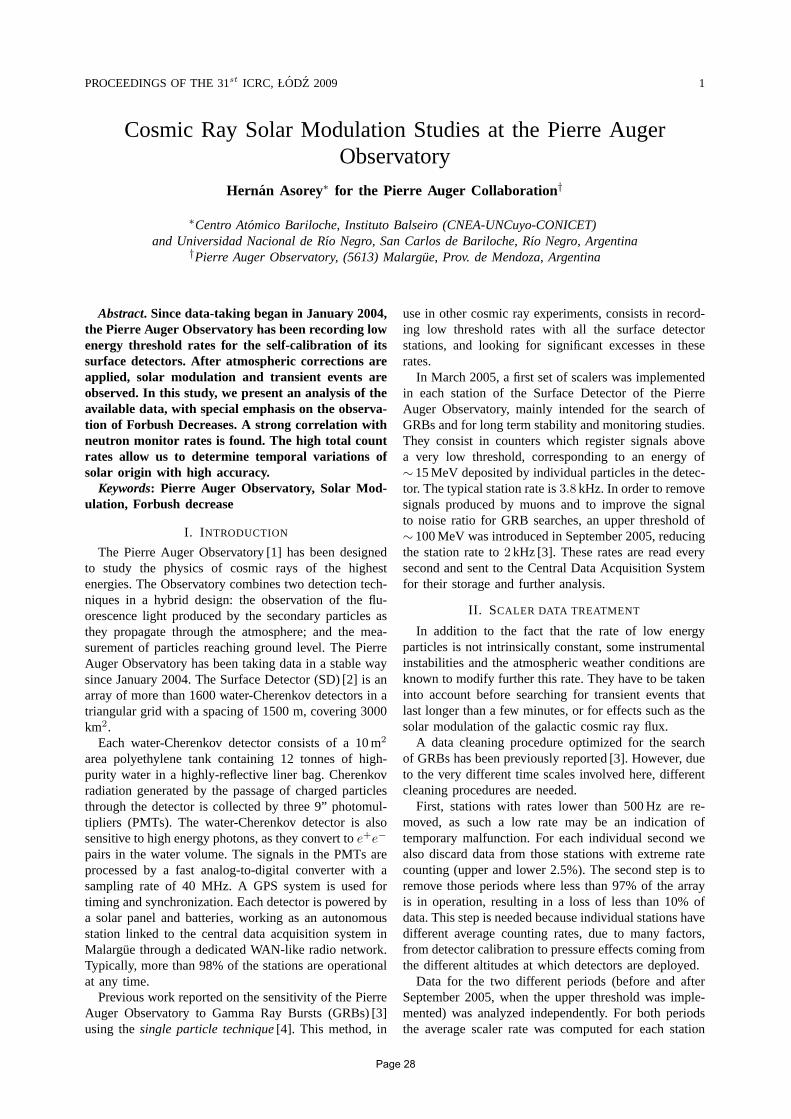
PROCEEDINGS OF THE 31st ICRC, ŁODZ 2009 1
Cosmic Ray Solar Modulation Studies at the Pierre AugerObservatory
Hernan Asorey∗ for the Pierre Auger Collaboration†
∗Centro Atomico Bariloche, Instituto Balseiro (CNEA-UNCuyo-CONICET)and Universidad Nacional de Rıo Negro, San Carlos de Bariloche, Rıo Negro, Argentina
†Pierre Auger Observatory, (5613) Malargue, Prov. de Mendoza, Argentina
Abstract. Since data-taking began in January 2004,the Pierre Auger Observatory has been recording lowenergy threshold rates for the self-calibration of itssurface detectors. After atmospheric corrections areapplied, solar modulation and transient events areobserved. In this study, we present an analysis of theavailable data, with special emphasis on the observa-tion of Forbush Decreases. A strong correlation withneutron monitor rates is found. The high total countrates allow us to determine temporal variations ofsolar origin with high accuracy.
Keywords: Pierre Auger Observatory, Solar Mod-ulation, Forbush decrease
I. I NTRODUCTION
The Pierre Auger Observatory [1] has been designedto study the physics of cosmic rays of the highestenergies. The Observatory combines two detection tech-niques in a hybrid design: the observation of the flu-orescence light produced by the secondary particles asthey propagate through the atmosphere; and the mea-surement of particles reaching ground level. The PierreAuger Observatory has been taking data in a stable waysince January 2004. The Surface Detector (SD) [2] is anarray of more than 1600 water-Cherenkov detectors in atriangular grid with a spacing of 1500 m, covering 3000km2.
Each water-Cherenkov detector consists of a 10 m2
area polyethylene tank containing 12 tonnes of high-purity water in a highly-reflective liner bag. Cherenkovradiation generated by the passage of charged particlesthrough the detector is collected by three 9” photomul-tipliers (PMTs). The water-Cherenkov detector is alsosensitive to high energy photons, as they convert toe+e−
pairs in the water volume. The signals in the PMTs areprocessed by a fast analog-to-digital converter with asampling rate of 40 MHz. A GPS system is used fortiming and synchronization. Each detector is powered bya solar panel and batteries, working as an autonomousstation linked to the central data acquisition system inMalargue through a dedicated WAN-like radio network.Typically, more than 98% of the stations are operationalat any time.
Previous work reported on the sensitivity of the PierreAuger Observatory to Gamma Ray Bursts (GRBs) [3]using thesingle particle technique[4]. This method, in
use in other cosmic ray experiments, consists in record-ing low threshold rates with all the surface detectorstations, and looking for significant excesses in theserates.
In March 2005, a first set of scalers was implementedin each station of the Surface Detector of the PierreAuger Observatory, mainly intended for the search ofGRBs and for long term stability and monitoring studies.They consist in counters which register signals abovea very low threshold, corresponding to an energy of∼15 MeV deposited by individual particles in the detec-tor. The typical station rate is3.8 kHz. In order to removesignals produced by muons and to improve the signalto noise ratio for GRB searches, an upper threshold of∼100 MeV was introduced in September 2005, reducingthe station rate to2 kHz [3]. These rates are read everysecond and sent to the Central Data Acquisition Systemfor their storage and further analysis.
II. SCALER DATA TREATMENT
In addition to the fact that the rate of low energyparticles is not intrinsically constant, some instrumentalinstabilities and the atmospheric weather conditions areknown to modify further this rate. They have to be takeninto account before searching for transient events thatlast longer than a few minutes, or for effects such as thesolar modulation of the galactic cosmic ray flux.
A data cleaning procedure optimized for the searchof GRBs has been previously reported [3]. However, dueto the very different time scales involved here, differentcleaning procedures are needed.
First, stations with rates lower than 500 Hz are re-moved, as such a low rate may be an indication oftemporary malfunction. For each individual second wealso discard data from those stations with extreme ratecounting (upper and lower 2.5%). The second step is toremove those periods where less than 97% of the arrayis in operation, resulting in a loss of less than 10% ofdata. This step is needed because individual stations havedifferent average counting rates, due to many factors,from detector calibration to pressure effects coming fromthe different altitudes at which detectors are deployed.
Data for the two different periods (before and afterSeptember 2005, when the upper threshold was imple-mented) was analyzed independently. For both periodsthe average scaler rate was computed for each station
Page 28

2 H. ASOREY et al. SOLAR MODULATION STUDIES
3500
3600
3700
3800
3900
Apr2005
May2005
Jun2005
Jul2005
Aug2005
Sep2005
Oct2005
Sca
ler
rate
[H
z]
Date (First period)
Auger scalers (cleaned data)
1900
2000
2100
Sep2005
Nov2005
Jan2006
Mar2006
May2006
Jul2006
Sep2006
Nov2006
Jan2007
Sca
ler
rate
[H
z]
Date (Second period)
Auger scalers (cleaned data)
1900
2000
2100
Jan2007
Mar2007
May2007
Jul2007
Sep2007
Nov2007
Jan2008
Mar2008
May2008
Sca
ler
rate
[H
z]
Date (Second period)
Auger scalers (cleaned data)
Fig. 1. Pierre Auger Observatory scaler rates after the datacleaning procedure described in the text, for the first period (before September2005, top), and for the second period (after September 2005, middle and bottom). Each data point is the average scaler rate over one hour.
over the lifetime of the detector. Detectors showingan RMS of more than twice the square root of therate were excluded, keeping more than 90% of thestations after this cut. Brief spurious events (such as highfrequency noise produced by lightnings) were removedby computing the average scaler rate for each detectorover a 5 minutes period in which data is available for
at least 4 minutes, removing the upper and lower 25%extreme values. Figure 1 shows the scaler data obtainedfor both the first and second scaler mode periods.
Atmospheric pressure variations are known to modifythe flux of secondary particles at ground level, due tothe different mass of atmosphere above the detector:an increase in the atmospheric pressure is correlated
Page 29
PROCEEDINGS OF THE 31st ICRC, ŁODZ 2009 3
1900
1950
2000
2050
30 Apr 03 May 06 May 09 May 12 May
870
865
860
Sca
ler
rate
[H
z]
Pre
ssure
[hP
a]
Date (2007, Second period)
Scaler countPressure
Fig. 2. Average scaler rate (solid line) and atmospheric pressure(dashed line, please note the reversed scale for pressure) for the firstten days of May of 2007.
with a reduction in the background rate. Figure 2 showsthe average scaler rate after the cleaning procedure,correlated with the flux of secondary particles at groundlevel, for the first ten days of May 2007, comparedwith the atmospheric pressure, as measured by severalweather stations monitoring the array.
The aforementioned correlation is observed and corre-sponds to about -0.27% (-0.36%) per hPa before (after)the upper threshold implementation. This also impliesthat an additional correction of 0.03% (0.04%) per metreof difference in altitude between stations has to beincluded.
3720
3725
3730
3735
3740
3745
3750
3755
3760
00 04 08 12 16 20 24
Av
erag
e sc
aler
rat
e (f
ull
dat
a se
t) [
Hz]
Local time (GMT-3) [hour]
cleaned dataPressure corrected
Fig. 3. Averaged scaler rates for the first period (before September2005) as a function of local hour of day (ARS, GMT-3) for the cleaned(dotted line) and for the atmospheric pressure corrected data (solidline).
III. SOLAR MODULATION
Figure 3 shows the average daily dependence. Afteratmospheric pressure correction, a 0.25% modulationremains, peaked at 17h45 UT (14h45 local time).
To show that the cleaned, pressure corrected, dataset is of relevance for solar studies [5], we comparethe Pierre Auger Observatory SD scaler rates with datafrom McMurdo neutron monitor of the Bartol Research
Institute [6]. Figure 5 shows the excellent agreementfound: Forbush decreases are clearly visible in the scalerdata for both periods. The upper threshold introduced onSeptember 2005, intended to optimize signal over noiseratio for GRB detection, is probably not the ideal onefor these studies, where the muon flux at ground levelmight be better correlated to the primary cosmic ray fluxthan the electron one.
As an example, Figure 4 shows the evolution of thescaler rates during the 11 Sep 2005 Forbush decrease [7].A 4% variation is observed, in agreement with the14% measured at McMurdo once taken into accountthe rigidity cut-off of 9.5 GeV at Malargue, Argentina(35.3oS, 69.3oW).
3550
3600
3650
3700
3750
3800
3850
05Sep
07Sep
09Sep
11Sep
13Sep
15Sep
17Sep
19Sep
21Sep
210
230
250
270S
cale
r ra
te [
Hz]
McM
urd
o r
ate
[Hz]
Date (2005, First period)
Auger scalersMcMurdo neutron monitor
Fig. 4. Averaged, cleaned and pressure corrected scaler rate for the11 Sep 2005 Forbush decrease, compared with the McMurdo neutrondetector rate (dotted line). A 4% variation is observed.
IV. CONCLUSIONS
Low energy radiation rates are registered with highstatistics at each surface detector station of the PierreAuger Observatory since March 2005. A data cleaningmethod, based on a previous one intended for thesearch of GRBs, has been implemented and optimizedto study solar modulation effects. After correcting forpressure, an excellent agreement with data from Mc-Murdo neutron monitor is found, evidencing the highsensitivity that water-Cherenkov detectors, operating inscaler mode, have for the detection and measurement ofForbush decreases and other transient events related withthe solar modulation of Galactic cosmic rays. Additionalanalyses of scaler rates at individual detectors and scalerthresholds optimisation are underway, together with lowenergy cosmic ray simulations in order to determine theenergies of the primaries responsible for the observedmodulation.
REFERENCES
[1] A. Watson [Pierre Auger Collaboration],“Highlights from thePierre Auger Observatory, the birth of the Hybrid Era”, Proc.30st ICRC, Volume 6, 67-78 (2007)
[2] I. Allekotte et al. [Pierre Auger Collaboration],“The SurfaceDetector System of the Pierre Auger Observatory”, NIM A586,409 (2008)
Page 30

4 H. ASOREY et al. SOLAR MODULATION STUDIES
3400
3500
3600
3700
3800
3900
Apr2005
May2005
Jun2005
Jul2005
Aug2005
Sep2005
Oct2005
230
250
270
Sca
ler
rate
[H
z]
McM
urd
o r
ate
[Hz]
Date (First period)
Auger scalers (corrected by pressure)McMurdo neutron monitor
1900
2000
2100
Sep2005
Nov2005
Jan2006
Mar2006
May2006
Jul2006
Sep2006
Nov2006
Jan2007
250
270
290
310
Sca
ler
rate
[H
z]
McM
urd
o r
ate
[Hz]
Date (Second period)
Auger scalers (corrected by pressure)McMurdo neutron monitor
1900
2000
2100
Jan2007
Mar2007
May2007
Jul2007
Sep2007
Nov2007
Jan2008
Mar2008
May2008
250
270
290
310
Sca
ler
rate
[H
z]
McM
urd
o r
ate
[Hz]
Date (Second period)
Auger scalers (corrected by pressure)McMurdo neutron monitor
Fig. 5. Pierre Auger Observatory scaler rates (solid lines)after cleaned procedure and atmospheric pressure correction, compared to McMurdoneutron detector data (dotted line), for both periods, before (top) and after September 2005 (middle and bottom).
[3] D. Thomas, [The Pierre Auger Collaboration],“Search forcoincidences with astrophysical transients in Pierre Auger Ob-servatory data”, Proc. 31st ICRC, Łodz (2009)
[4] S. Vernetto, “Detection of gamma-ray bursts in the 1-GeVto 1-TeV energy range by ground based experiments”,Astropart. Phys. 13, 75 (2000), [arXiv:astro-ph/9904324]
[5] L. Gleeson and W. I. Axford“Solar Modulation of GalacticCosmic Rays”, Astrophys. Jour.154, 1011-1026 (1968)
[6] Bartol Research Institute,“McMurdo Neutron Monitor Data”,http://neutronm.bartol.udel.edu/∼pyle/bri table.html
[7] National Geophysical Data Center, ftp://ftp.ngdc.noaa.gov/
Page 31

PROCEEDINGS OF THE 31st ICRC, ŁODZ 2009 1
Investigation of the Displacement Angle of the Highest EnergyCosmic Rays Caused by the Galactic Magnetic Field
B. M. Baughman∗, for the Pierre Auger Collaboration†∗Ohio State University, 191 W. Woodruff Ave., Columbus, OH 43210-1061, United States
†Observatorio Pierre Auger, Av. San Mart ın Norte 304, (5613) Malargue, Mendoza, Argentina
Abstract. Ultra-high energy cosmic rays (UHECR)are deflected by magnetic fields during their prop-agation. Different theoretical parameterizations ofthe Galactic magnetic field are examined using anumerical tool which simulates their propagationthrough models of these fields. We constrain thepossible parameter space of the models by comparingdata on UHECR obtained with the Pierre AugerObservatory with the results of the simulations.
Keywords: Auger, magnetic field, constraints
I. INTRODUCTION
Current knowledge on the strength and shape of theGalactic magnetic field is limited [1], [2], [3], [4], [5],[6], [7]. While there are hints [3], [4], [5], [6], [7] at theform and magnitude of the regular component of theGalactic magnetic field there is currently no consensuson its general form or magnitude. Presented here is amethod for determining regions of magnetic field modelparameter space which are compatible with a givenset of assumptions. Combining this method with com-plementary methods [8] employing multi-wavelengthobservations will improve the global delimiting power.This method is applied to determine regions of parameterspace for two Galactic magnetic field models and undertwo dramatically different sets of assumptions: 1) thePierre Auger Observatory [9] (Auger) anisotropy resultwith a pure proton composition and 2) Centaurus A asa dominant source with a pure iron composition.
II. DATA SET
This analysis uses data recorded by the southern siteof the Auger Observatory between 1 January 2004 and31 March 2009 with energies greater than 55 EeV andzenith angles smaller than 60.
III. GALACTIC MAGNETIC FIELD MODELS
Logarithmic symmetric spiral field models [1], [10]are used to model the large scale regular Galactic mag-netic field in this work. Axisymmetric [Bi-symmetric](denoted herein as ASS * [BSS *]) fields exhibit [anti-]symmetry under rotations of π around the Galacticpole. Fields [anti-]symmetric under reflection across theGalactic plane are denoted with *SS S [*SS A]. Aprecise description of the models used, including thenominal parameter values, is given by Harari et al. [1].These models are likely not a complete description
of the Galactic magnetic field [2], [3], [5], [7], [11].There is evidence of turbulent and halo fields in the
Galaxy [2], [3], [4], [7], [6], [12] and others [13], [14],[11]. Furthermore, extra-galactic magnetic fields [15],[16], [17] will also have an effect on the results of thiswork. However, logarithmic symmetric spirals representa priori reasonable models for the functional form ofthe regular component of the Galactic magnetic field[4], [14]1. Here we present results using two logarithmicsymmetric spiral models: BSS S and ASS A.
IV. METHOD
Regions of compatible parameter space are deter-mined by testing the Auger Observatory data under aset of assumptions. The general method presented hererequires a hypothesis which defines the following: 1)A charge for each observed event, 2) a catalog whichtraces the true source distribution and parameters forcorrelation (Ψmax), 3) a model for the magnetic field.A region of interest in parameter space is then griddedand all events are backtracked through the model ateach grid point. The region around the direction of theexiting velocity vector for each event is then searched forthe nearest catalog object. Finally, the number of events(Ncorr) correlating (Ψ ≤ Ψmax) with the hypothesizedsource catalog are interpreted relative to the numberof correlations determined without backtracking throughthe magnetic field model.The statistical significance of Ncorr is determined
by assuming that the number of correlations with thenon-backtracked arrival directions (N0
corr) is an estimateof the true number of correlations for the parametersgiven. We take the number of correlations with thenon-backtracked arrival directions as an estimate of themean of a Poisson distribution. We expect this to bea conservative estimator of the true probability massfunction2. A region of compatibility is defined as lyingcentered on the mean and containing 68% of randomNcorr values sampled from this distribution. Scan pointswith Ncorr values lying outside this region are consid-ered incompatible with the full set of assumptions (field,source, and composition). Figure 1 shows two Poissondistributions with shaded regions found using the abovemethod.
1The results presented herein may depend on the specifics ofturbulent, halo, or extra-galactic magnetic fields which are poorlyconstrained, as such the effects of such fields have been ignored infavor of presenting a clear description of the method used.2We have verified this by smearing the data with a 2D gaussian and
examining simple Monte Carlo realizations.
Page 32

2 B. M. BAUGHMAN et al. UHECR DEFLECTIONS BY THE GALACTIC MAGNETIC FIELD
TABLE I: Example Assumptions
VCV CenA
Composition Pure proton Pure ironSource Distribution VCV Catalog Centaurus A
Correlation Scale (Ψmax) 3.1 15Minimum Energy (Emax) 55 EeV 55 EeVPoisson Mean (N0
corr) 27 9
V. EXAMPLES
Here we present two examples for clarity. Eachexample explicitly assumes a composition, a sourcedistribution, and angular correlation window which canbe found in Table I.The first example is inspired by the Auger Observa-
tory anisotropy result [9] and will be referred to as theVCV example throughout. By correlating the arrival di-rections of UHECR with Active Galactic Nuclei (AGN)from the Veron Catalog of Quasars & AGN, 12th Edition[18] (VCV catalog) and comparing the results with whatone would expect from a truly isotropic source distribu-tion, the Auger Observatory found that their observationswere consistent with a sampling of a distribution similarto the VCV catalog. The Auger Observatory scannedover three parameters: maximum redshift (zmax), max-imum angular correlation scale (Ψmax), and minimumenergy (Emin) finding the strongest correlation signalfor zmax = 0.018, Ψmax = 3.1 and Emax = 55EeV (equivalent to 57 EeV as reported in [9] due toa small change in our energy calibration). This analysisuses VCV catalog objects with a redshift ≤ 0.018.The second example assumes that Centaurus A (Cen
A) is the dominant source in a region centered aroundit. This example is referred to as the Cen A examplethroughout. We have arbitrarily chosen Ψmax = 15.Both examples use the minimum energy (E > 55
EeV) found in the Auger Observatory anisotropy result[19], [20]. Compatible regions for both BSS S andASS A Galactic magnetic field models are presented.Neither the overall strength nor the scale height of theGalactic magnetic field is well constrained [1], [2], [4],[10]. Thus for each of the two models two parametersare varied: the strength of the field in the solar vicinity(B) and the dominant scale height (z1). B is variedfrom −2.5 µG to 2.5 µG in steps of 0.01 µG and from0.05 kpc to 3.05 kpc in z1 in steps of 0.1 kpc.
VI. RESULTS
A. VCV
Figures 2a and 2b show the regions of B- z1
parameter space compatible with the Auger Observa-tory anisotropy result. The regions of compatibility aredefined using the method described in Sec. IV above.This example uses a N0
corr = 27 to define the mean ofthe Poisson distribution from which we determine ourcompatibility regions. The shaded regions correspond tothe similarly shaded regions in Fig. 1a. There are somegeneral features to both field models which should be
noted. First, z1 is not well constrained as both modelshave regions compatible with the Auger Observatoryanisotropy result extending across all reasonable scalelengths. Second, that connected statistically compatibleregions lie within the range over which B is varied.There is marked difference in the compatible pa-
rameter space between ASS A (Fig.2a,) and BSS S(Fig.2b) models. ASS A has large connected compatibleregions only for a small range in B centered aroundzero. Furthermore, no regions appear to improve thenumber of correlations, thus it is likely that the com-patible regions are simply where the correlation withthe arrival directions have yet to be destroyed. ASS Ais compatible only with |N| < 1 µG which is lowerthan the expected value [1], [3], [4], [5]. Overall, theASS A model is incompatible with the VCV correlationhypothesis in the regions deemed acceptable due to otherconstraints.The connected compatible (gray and dark gray) region
for BSS S model is much larger and extends over asignificant range in B. Furthermore, extended regionsexist where Ncorr is above 27, the nominal value,indicating candidate models where the correlations arepreserved and new correlations are made.
B. Cen A
Figures 3a and 3b show the regions of B- z1
parameter space compatible with the Cen A hypothesis.This example uses a N0
corr = 9 to define the mean ofthe Poisson distribution from which we determine ourcompatibility regions. The shaded regions correspond tothe similarly shaded regions in Fig. 1b.This parameter space shares features with the previous
example, mainly that z1 is not well constrained andcompatible regions of parameter space tend to preferpositive field strengths. The most striking feature of thisparameter space is the very limited range in field strengthcompatible with the underlying hypothesis; both modelsrequire a field strength in the solar vicinity of less than0.24 µG.
VII. CONCLUSION
Presented is a method which can be used to determinecompatible regions of parameter space for magnetic fieldmodels using UHECRs. Regions of parameter space areshown for two common Galactic magnetic field modelscompatible with either the Auger Observatory anisotropyresults and a pure proton composition or with Cen Aas a dominant source on a 15 scale with a pure ironcomposition. These regions are determined through astatistical comparison between the results of correlationsbetween Auger Observatory data and either the VCVcatalog or Cen A and similar correlations between par-ticles backtracked through BSS S and ASS A Galacticmagnetic field models.By assuming a pure proton composition and VCV cat-
alog correlation parameters, it is found that the ASS Amodel has a smaller compatible parameter space while
Page 33
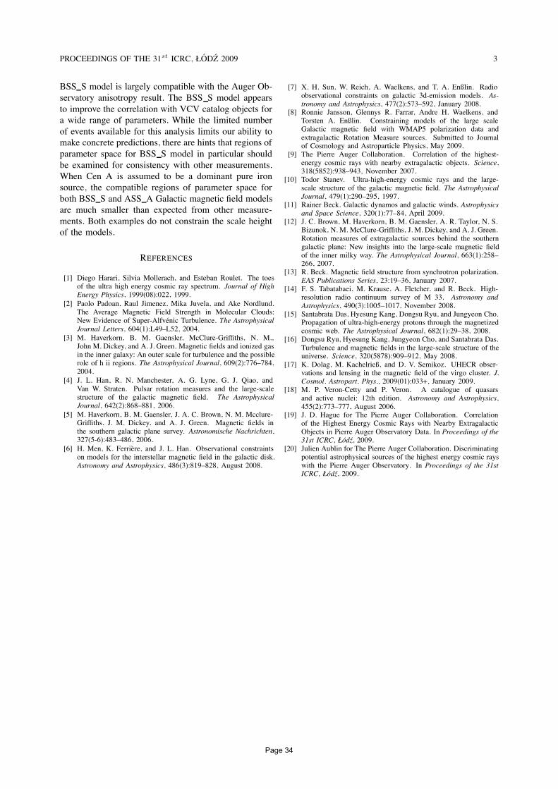
PROCEEDINGS OF THE 31st ICRC, ŁODZ 2009 3
BSS S model is largely compatible with the Auger Ob-servatory anisotropy result. The BSS S model appearsto improve the correlation with VCV catalog objects fora wide range of parameters. While the limited numberof events available for this analysis limits our ability tomake concrete predictions, there are hints that regions ofparameter space for BSS S model in particular shouldbe examined for consistency with other measurements.When Cen A is assumed to be a dominant pure ironsource, the compatible regions of parameter space forboth BSS S and ASS A Galactic magnetic field modelsare much smaller than expected from other measure-ments. Both examples do not constrain the scale heightof the models.
REFERENCES
[1] Diego Harari, Silvia Mollerach, and Esteban Roulet. The toesof the ultra high energy cosmic ray spectrum. Journal of HighEnergy Physics, 1999(08):022, 1999.
[2] Paolo Padoan, Raul Jimenez, Mika Juvela, and Ake Nordlund.The Average Magnetic Field Strength in Molecular Clouds:New Evidence of Super-Alfvenic Turbulence. The AstrophysicalJournal Letters, 604(1):L49–L52, 2004.
[3] M. Haverkorn, B. M. Gaensler, McClure-Griffiths, N. M.,John M. Dickey, and A. J. Green. Magnetic fields and ionized gasin the inner galaxy: An outer scale for turbulence and the possiblerole of h ii regions. The Astrophysical Journal, 609(2):776–784,2004.
[4] J. L. Han, R. N. Manchester, A. G. Lyne, G. J. Qiao, andVan W. Straten. Pulsar rotation measures and the large-scalestructure of the galactic magnetic field. The AstrophysicalJournal, 642(2):868–881, 2006.
[5] M. Haverkorn, B. M. Gaensler, J. A. C. Brown, N. M. Mcclure-Griffiths, J. M. Dickey, and A. J. Green. Magnetic fields inthe southern galactic plane survey. Astronomische Nachrichten,327(5-6):483–486, 2006.
[6] H. Men, K. Ferriere, and J. L. Han. Observational constraintson models for the interstellar magnetic field in the galactic disk.Astronomy and Astrophysics, 486(3):819–828, August 2008.
[7] X. H. Sun, W. Reich, A. Waelkens, and T. A. Enßlin. Radioobservational constraints on galactic 3d-emission models. As-tronomy and Astrophysics, 477(2):573–592, January 2008.
[8] Ronnie Jansson, Glennys R. Farrar, Andre H. Waelkens, andTorsten A. Enßlin. Constraining models of the large scaleGalactic magnetic field with WMAP5 polarization data andextragalactic Rotation Measure sources. Submitted to Journalof Cosmology and Astroparticle Physics, May 2009.
[9] The Pierre Auger Collaboration. Correlation of the highest-energy cosmic rays with nearby extragalactic objects. Science,318(5852):938–943, November 2007.
[10] Todor Stanev. Ultra-high-energy cosmic rays and the large-scale structure of the galactic magnetic field. The AstrophysicalJournal, 479(1):290–295, 1997.
[11] Rainer Beck. Galactic dynamos and galactic winds. Astrophysicsand Space Science, 320(1):77–84, April 2009.
[12] J. C. Brown, M. Haverkorn, B. M. Gaensler, A. R. Taylor, N. S.Bizunok, N. M. McClure-Griffiths, J. M. Dickey, and A. J. Green.Rotation measures of extragalactic sources behind the southerngalactic plane: New insights into the large-scale magnetic fieldof the inner milky way. The Astrophysical Journal, 663(1):258–266, 2007.
[13] R. Beck. Magnetic field structure from synchrotron polarization.EAS Publications Series, 23:19–36, January 2007.
[14] F. S. Tabatabaei, M. Krause, A. Fletcher, and R. Beck. High-resolution radio continuum survey of M 33. Astronomy andAstrophysics, 490(3):1005–1017, November 2008.
[15] Santabrata Das, Hyesung Kang, Dongsu Ryu, and Jungyeon Cho.Propagation of ultra-high-energy protons through the magnetizedcosmic web. The Astrophysical Journal, 682(1):29–38, 2008.
[16] Dongsu Ryu, Hyesung Kang, Jungyeon Cho, and Santabrata Das.Turbulence and magnetic fields in the large-scale structure of theuniverse. Science, 320(5878):909–912, May 2008.
[17] K. Dolag, M. Kachelrieß, and D. V. Semikoz. UHECR obser-vations and lensing in the magnetic field of the virgo cluster. J.Cosmol. Astropart. Phys., 2009(01):033+, January 2009.
[18] M. P. Veron-Cetty and P. Veron. A catalogue of quasarsand active nuclei: 12th edition. Astronomy and Astrophysics,455(2):773–777, August 2006.
[19] J. D. Hague for The Pierre Auger Collaboration. Correlationof the Highest Energy Cosmic Rays with Nearby ExtragalacticObjects in Pierre Auger Observatory Data. In Proceedings of the31st ICRC, Łodz, 2009.
[20] Julien Aublin for The Pierre Auger Collaboration. Discriminatingpotential astrophysical sources of the highest energy cosmic rayswith the Pierre Auger Observatory. In Proceedings of the 31stICRC, Łodz, 2009.
Page 34

4 B. M. BAUGHMAN et al. UHECR DEFLECTIONS BY THE GALACTIC MAGNETIC FIELD
10 20 30 40 50
Value
1
2
3
4
5
6
7
8
PercentProbability
6.9% 12.7%42.9% 23.0% 14.5%
Probability Mass Function for Mean=27
(a) Poisson distribution corresponding to the VCV example.
2 4 6 8 10 12 14 16
Value
2
4
6
8
10
12
14
PercentProbability
5.5% 15.2% 49.9% 22.0% 7.4%
Probability Mass Function for Mean=9
(b) Poisson distribution corresponding to the CenA example.
Fig. 1: Circles represent the percent probability of obtaining each value. Regions shaded to indicate the portion ofprobability space occupied by corresponding regions in Figs. 2 and 3
0.5 1.0 1.5 2.0 2.5 3.0
Scale Height (kpc)
−2
−1
0
1
2
Field
Strength
inSolarVicinity(µG)
Compatibility with VCV and 2007 Parameters in ASS_A
(a) ASS A Galactic magnetic field model.
0.5 1.0 1.5 2.0 2.5 3.0
Scale Height (kpc)
−2
−1
0
1
2
Field
Strength
inSolarVicinity(µG)
Compatibility with VCV and 2007 Parameters in BSS_S
(b) BSS S Galactic magnetic field model.
Fig. 2: Regions shaded in: white has [0-19), light gray has [19,22), gray has [22,28), and dark gray has [28,32)correlations. The ASS A model reaches a maximum of 28 correlations while the BSS S model has a maximumof 29.
0.5 1.0 1.5 2.0 2.5 3.0
Scale Height (kpc)
−2
−1
0
1
2
Field
Strength
inSolarVicinity(µG)
Compatibility with 15 of CenA in ASS_A
(a) ASS A Galactic magnetic field model.
0.5 1.0 1.5 2.0 2.5 3.0
Scale Height (kpc)
−2
−1
0
1
2
Field
Strength
inSolarVicinity(µG)
Compatibility with 15 of CenA in BSS_S
(b) BSS S Galactic magnetic field model.
Fig. 3: Regions shaded in: white has [0-4), light gray has [4,6), gray has [6,10), and dark gray has [10,13)correlations. The ASS A model reaches a maximum of 10 correlations while the BSS S model has a maximumof 13.
Page 35

PROCEEDINGS OF THE 31st ICRC, ŁODZ 2009 1
Search for coincidences with astrophysical transients in PierreAuger Observatory data
David Thomas∗ for the Pierre Auger Collaboration†
∗Colorado State University, Fort Collins CO, USA†Pierre Auger Observatory, Av. San Martin Norte 304 (5613) Malargue, Prov. de Mendoza, Argentina
Abstract. We analyse extensive air shower datacollected by the Pierre Auger Observatory to searchfor coincidences between the arrival directions ofultra-high energy cosmic rays and the positions ofgamma-ray bursts. We also analyse the trigger ratedata from individual surface detector stations tosearch for an increase of the average trigger rateover the entire surface detector array in correlationwith gamma-ray bursts.
Keywords: Auger GRB transients
I. INTRODUCTION
Since their discovery at the end of the 1960s [1],gamma-ray bursts (GRBs) have been of high interestto astrophysics. A GRB is characterised by a suddenemission of gamma rays during a very short period oftime, typically lasting between 0.1 and 100 seconds.The equivalent isotropic energy emission during a burstis typically between 1051 and 1055 ergs. Good sourcecandidates for these bursts are the merger of neutronstars, for short bursts of less than 2 seconds, and core-collapse supernovae type Ib/c, for long bursts. See [2]for a recent review.
A large data set of GRBs was provided by the BATSEinstrument on board the Compton Gamma Rays Ob-servatory (1991-2000). More GRBs were then detectedby BEPPO-SAX (1997-2002) and HETE (2001-2006).Currently, GRBs are registered by Swift, INTEGRAL,IPN, the Fermi Gamma Ray Telescope. In the lastseveral years, afterglows have been observed allowingus to precisely measure their direction, and giving usa much better understanding of the GRB phenomena.Most observations have however been done below a fewGeV of energy, and the highest energy observations havebeen around 10 GeV [3].
Using the recently completed surface detector array(SD) of the Pierre Auger Observatory [4], [5], an arrayof more than 1600 water Cherenkov detectors, we lookfor evidence of GRBs in our data with two separatetechniques. For the first study, we use the regular Augercosmic ray (CR) events to look for an excess of ultra-high energy CRs (UHECRs) in the direction of GRBs.We presented a similar analysis at the last ICRC [6].
In the second study, the “single particle technique” [7]is used with low-level trigger rate data from individualsurface detector stations to look for a possible extensionof the photon spectrum of GRBs in the 1 GeV –1 TeV range, which is not well-studied by satellites.
When photons in this energy range reach the atmo-sphere, they produce cosmic ray cascades that can bedetected, although the energies are too low to produce ashower detectable at ground level, even at high altitudes.However, a lot of these photons are expected to arriveduring a GRB in a short period of time, which wouldbe detectable as an overall increase of the trigger rate inall the detectors [8] in the array.
This technique was first applied in EAS-TOP [7],using scintillators, and subsequently in INCA [9] andARGO [10], using scintillators and RPCs, respectively.The main advantage to using water Cherenkov detec-tors [11], [12] is their sensitivity to photons, whichrepresent up to 90% of the secondary particles at groundlevel for high energy photon initiated showers such asthese. This study is also an update to one we presentedat the last ICRC [13].
II. SEARCH FOR COINCIDENCEOF UHECRS AND GRBS
For this analysis, we use CR data collected with thePierre Auger Observatory surface detector. We considerevents from 1 January 2004 to 31 March 2009, passingquality criteria discussed elsewhere [14] with zenithangle θ < 60. We perform no energy cut on the data.
We use a catalogue of 511 GRBs [15] observedwith an accuracy better than 1 compiled using dataprimarily from the Swift mission complemented bymeasurements from additional GRB observing satellites,including HETE, INTEGRAL, IPN, and Fermi. Out ofthe total GRB sample, 115 bursts are within the field ofview at the time of their bursts, i.e. θGRB < 60.
We look for excess CRs in the direction of GRBsby determining the differences in the observation timesof the GRBs and the arrival times of CR events thatfall within a window of radius ψ around each GRBposition. We compare this with the expected rate ofevents, which is calculated in the same manner, usingthe declination band of width 2ψ around the GRB(excluding the circular window around the GRB). Theexpected rate of events is normalized by multiplying bythe on-source solid angle of the window divided by thetotal solid angle (declination band minus the window.)
A value of ψ = 2 corresponds roughly to the angularresolution when all SD events are used. To be consistentwith the previous analysis, we also used a window ofψ = 5. The results are presented in Figure 1. There
Page 36

2 DAVID THOMAS et al. SEARCH FOR TRANSIENT COINCIDENCES WITH AUGER DATA
Fig. 1. Number of CR events as a function of the difference betweenthe GRB time and the CR arrival time, for windows of ψ = 2 (top)and ψ = 5 (bottom). Data falling within the windows of radius ψare indicated by the points. The expected rate of events is indicatedby the solid line. For clarity, statistical errors are only shown for thecircular windows.
is no evidence for an excess of CRs coming from thedirection of GRBs.
III. SINGLE PARTICLE TECHNIQUE
A. Scaler data
In addition to the regular data acquisition systemused to detect cosmic rays, the surface detectors areequipped with scalers, simple counters that can be setlike any other trigger. They record the counting rates ofsignals more than 3 ADC counts above baseline and lessthan 20 ADC counts, or approximately between 15 and100 MeV deposited in the detector. This trigger levelhas been set to optimise the signal to noise ratio giventhe expected signal extracted from simulations [16], andthe background signal derived from real data histograms.With these cuts, the average scaler rate over the array isof about 2 kHz per detector. Note that the scaler data iscompletely separate from the regular cosmic ray data, asit only reports trigger rates in individual surface detectorstations, and cannot be used to reconstruct cosmic rayevents.
To use the scaler data, it must be cleaned. Individualdetectors often experience increases in their countingrates due to noisy or unstable baseline, unstable PMTs,or bad calibration. Detectors with less than 500 Hz ofscaler counts are discarded. This removes a few badlycalibrated detectors. Additionally, for each individualsecond, only 95% of detectors are kept, removing the5% with extreme rate counting (2.5% on each side).This removes outliers which could impact the averagerate of a specific second, without affecting the GRBdetection capability, as GRB would appear as an increaseof counting rates in all the detectors.
One then needs to have the array operating properly.Suddenly losing a significant fraction of the array willcause jumps in the scaler rate, as this rate is not uniformover the whole Observatory. Consequently, we only usedata periods for which more than 97% of the stationsare operating. This keeps 83% of the data. We alsorequire at least 5 continuous minutes with data, to beable to compute reasonable averages and see eventualbursts. This removes 12% of the remaining data set.Some artificial bursts are found in the cleaned scalerdata set due to lightning strikes. Therefore, we do notuse the data taken during lightning storms, removing 4%of the data. This scaler data cleaning process is differentfrom the one used in the analysis of the modulation ofsolar CRs [17] due to the difference in time scales.
B. σ − δ method
To search for bursts, the average rate for each secondas well as a longer term average rate are computed. Asa burst would produce a similar increase in all stations,a good estimator of the average rate for each second,r, is the median of the rates of all the stations. It ismuch less sensitive to misbehaving detectors than thearithmetic average. Then, to estimate a long term averageR, a σ − δ method is used with σ = 0 and δ = 0.1 Hz,meaning that every second the average rate R is movedby 0.1 Hz towards the current rate r. After 30 secondsof data, this average converges to the expected averagevalue, and one can compute the variation ∆ of the rater of a specific second using:
∆ =r −R√
r/N
where N is the number of active detectors at that second.The ∆ parameter can be used directly to search for
bursts, and its histogram can be seen in Figure 2. Theunderlying Gaussian has a width of 1.4. It would have awidth of 1 if the arriving flux of particle was poissonian,the fluctuations of each detector were independent, thebaselines of the detectors were not fluctuating, and theσ−δ method gave the true average at each moment. Onesigma of deviation corresponds roughly to 1.5 particlesper detector, i.e. a flux at ground level of 0.15 m−2 s−1.
C. Search for self-triggered bursts
Once all the cuts defined above have been applied, atotal of 70% of the data period (21 September 2005 -31 March 2009) is available for a search for bursts. Theresulting ∆ histogram is shown in Figure 2.
Only three candidate bursts are observed significantlyoutside of the Gaussian distribution. To be related toa GRB, the increase of the rate should be uniformlydistributed over all the detectors. One can thereforecheck that each individual detector has on average anincrease at the moment of the burst with respect of theprevious seconds. The observed outliers do not presentsuch a feature, as only a fraction of the array sees asignificant excess. We show in Figure 3 the histogram
Page 37

PROCEEDINGS OF THE 31st ICRC, ŁODZ 2009 3
1
103
106
-10 -5 0 5 10 15
Cou
nts
Scaler rate deviation ∆
Fig. 2. Histogram of the deviations ∆ of the scaler counting rates.The distribution is Gaussian with a width of 1.4. Three candidate burstsare present above 10σ which we looked at more closely to determineif they are due to GRBs.
of the difference of the scaler rate from the average overthe previous seconds for one of these candidate bursts.Most of the rate increase is attributable to a small portionof the array. The excess is therefore artificial and mustbe due to lightning. All other candidate bursts displaythis same attribute.
1
10
100
-400 0 400 800 1200
Num
ber
of d
etec
tors
Scaler rate difference (r-R)
Fig. 3. Histogram of the difference of scaler rates from the averageover the previous seconds for one of the three candidate bursts. Thescaler rate increase is due to an increase in the rate for a small fractionof the array. Thus, this candidate burst is due to lightning. The othercandidate bursts display this same characteristic.
D. Search for satellite-triggered bursts
In the period studied, 129 bursts detected by satellitesoccurred in the field of view of Auger (θGRB < 90).For all these bursts, the scaler data were checked within100 seconds of the burst for a one second excess. Noexcesses were found and the resulting 5 σ fluence limitswere computed assuming a GRB spectra dN/dE ∝ E−2
in the 1 GeV – 1 TeV energy range (as in [9]). The limitsare reported in Figure 4.
1
10
100
-6 -4 -2 0 2 4 6
Cou
nts
Scaler rate deviation ∆
-6
-5
-4
-3
-2
0 10 20 30 40 50 60
Log
Flu
ence
(er
g.cm
-2)
GRB zenith angle [deg]
1 sec burst fluence limit
Fig. 4. Top: histogram of the deviations ∆ of the scaler counting rateswithin 100 seconds of the bursts reported by satellites. No significantexcess is observed. Bottom: 5-σ fluence limits in the 1 GeV – 1 TeVenergy range from Auger for these bursts, for a single second burst,assuming a spectral index of -2.
IV. CONCLUSION
We have used the cosmic ray data from the surfacedetector of the Pierre Auger Observatory to search forcosmic rays that correlate with the time and position ofGRBs. No such correlations were found.
As a separate analysis, we used the scaler data tolook for increases in the average trigger rate of thesurface detectors, which would indicate the occurrenceof a GRB. No burst with characteristics similar to thoseexpected for GRBs was observed.
Fluence limits of up to 3.4× 10⁻⁶ erg cm−2 (depend-ing on the burst zenith and duration), were deduced forthe 1 GeV – 1 TeV energy range. Note that modelsdo not generally favor fluences above 10−6 erg cm−2 inthe energy range considered [18], [19]. To reach such asensitivity, a detector is needed that covers a significantsurface at higher altitude. Such a detector could be anextension of the LAGO project [20] that has been takingdata since 2007.
Page 38

4 DAVID THOMAS et al. SEARCH FOR TRANSIENT COINCIDENCES WITH AUGER DATA
REFERENCES
[1] R. W. Klebesadel, I. B. Strong and R. A. Olson, “Observations ofGamma-Ray Bursts of Cosmic Origin”, Astrophys. J. 182, L85(1973).
[2] P. Meszaros, Reports on Progress in Physics 69, 2259 (2006).[3] A. A. Abdo [The Fermi LAT and Fermi GBM Collaborations],
“Fermi Observations of High-Energy Gamma-Ray Emissionfrom GRB 080916C”, Science 323, 1688 (2009).
[4] J. Abraham [Pierre Auger Collaboration], “Properties and per-formance of the prototype instrument for the Pierre AugerObservatory”, Nucl. Instrum. Meth. A 523, 50 (2004).
[5] I. Allekotte et al, “The Surface Detector System of the PierreAuger Observatory”, Nucl. Instrum. Meth. A 586, 409 (2008).
[6] L. Anchordoqui [Pierre Auger Collaboration], “Search for Co-incidences in Time and Arrival Direction of Auger Data withAstrophysical Transients”, Proc. 30th ICRC, Merida 4, 437(2007).
[7] M. Aglietta et al, “Search for gamma ray bursts at photonenergies E ≤ 10 GeV and E ≥ 80 TeV”, Astrophys. J. 469,305 (1996).
[8] S. Vernetto, “Detection of gamma-ray bursts in the 1 GeV to1 TeV energy range by ground based experiments”, Astropart.Phys. 13, 75 (2000).
[9] R. Cabrera et al, “Search for GeV GRBs with the INCAexperiment”, Astron. Astrophys. Suppl. Ser. 138, 599 (1999).
[10] T. Di Girolamo et al, “Search for Gamma Ray Bursts with theARGO-YBJ detector”, Proc. 30th ICRC, Merida 3, 1163 (2007).
[11] D. Allard [Pierre Auger Collaboration], “Detecting gamma-raybursts with the Pierre Auger Observatory using the single particletechnique”, Proc. 29th ICRC, Pune (2005).
[12] X. Bertou and D. Allard, “Detection of GRB with waterCherenkov detectors”, Nucl. Instrum. Meth. A 553, 299 (2005).
[13] X. Bertou [Pierre Auger Collaboration], “Search for Gamma RayBursts using the single particle technique at the Pierre AugerObservatory”, Proc. 30th ICRC, Merida 4, 441 (2007).
[14] J. Abraham et al, “Correlation of the highest-energy cosmic rayswith the positions of nearby active galactic nuclei”, Astropart.Phys. 29, 188 (2008).
[15] J. Greiner, http://www.mpe.mpg.de/∼jcg/, April, 2009.[16] D. Allard [Pierre Auger Collaboration], “Detecting gamma-ray
bursts with the Pierre Auger observatory using the single particletechnique”, Nucl. Phys. Proc. Suppl. 165, 110 (2007).
[17] H. Asorey [Pierre Auger Collaboration], “Cosmic Ray SolarModulation Studies at the Pierre Auger Observatory”, Proc. 31st
ICRC, Łodz, (2009).[18] N. Guptan and B. Zhang, “Prompt Emission of High Energy
Photons from gamma-ray Bursts”, MNRAS 380, 78 (2007).[19] Y. Fan et al, “High-energy afterglow emission from Gamma-ray
Bursts”, MNRAS 384, 1483 (2008).[20] D. Allard et al, Proc. 31st ICRC, Łodz, (2009) #1413.
Page 39

PROCEEDINGS OF THE 31st ICRC, ŁODZ 2009 1
An alternative method for determining the energy of hybrid eventsat the Pierre Auger Observatory
Patrick Younk∗ for the Pierre Auger Collaboration†
∗Colorado State University, Fort Collins, Colorado 80523, United States†Observatorio Pierre Auger, Av. San Martin Norte 304, (5613) Malargue, Mendoza, Argentina
Abstract. An important feature of the Pierre AugerObservatory is the detection of hybrid events; i.e.,extensive air showers simultaneously detected with atleast one water-Cherenkov detector (surface detector)and one fluorescence telescope. Here we describean alternative method of estimating the energy ofthese events. The shower axis is determined usingdata from both detector systems. The shower energyis determined from the integrated surface detectorsignals and the distance of each detector from theshower axis. The energy estimate is facilitated bythe characterisation of an average lateral distributionfunction as a function of the shower energy andzenith angle. The method requires only the signalfrom one surface detector. Thus, it is useful forestimating the energy of hybrid events for whichthe geometry cannot be estimated with the surfacedetectors alone and the longitudinal profile measuredby the fluorescence telescopes is not well determined.In the energy range 0.4 < E < 1 EeV, the methoddoubles the number of hybrid events that can begiven an energy estimate. The statistical uncertaintyof this energy estimate is dependent on the showerenergy and geometry. For events with energy greaterthan 0.4 EeV, the median statistical uncertainty is26% and the 90% quantile is 44%.
Keywords: Extensive air shower reconstruction
I. INTRODUCTION
The Pierre Auger Observatory detects the highestenergy cosmic rays with over 1600 water-Cherenkovdetectors arranged as an array on a triangular grid with1500 m spacing. The 3000 km2 array is collectivelycalled the surface detector array (SD). The SD is over-looked by the fluorescence detector (FD), which consistsof 24 fluorescence telescopes grouped in units of 6 atfour locations on the periphery of the SD. The AugerObservatory was designed so that events recorded bythe FD are generally recorded also by the SD. Cosmicray showers detected with both detectors are referred toas hybrid events.
There are two standard methods for reconstructing thegeometry (shower axis) and energy of hybrid events.The first method, SD reconstruction, uses only data fromSD stations. The shower geometry and station signal at1000 m from the shower axis S(1000) are estimated.The shower energy is derived from S(1000) and zenithangle through a set of calibration equations (e.g., [1]).
The requirements for SD reconstruction are that theintersection of the shower axis with the ground (coreposition) be contained within an equilateral triangle ofoperating stations and that at least three stations recordshower particles [2].
The second method, hybrid reconstruction, is bestdescribed as a two-step sequence. First, data from theFD telescopes and one SD station are used to estimatethe shower geometry [3]. This estimate is referred toas the hybrid geometry. Second, the hybrid geometryand the signal levels recorded by the FD telescopes areused to determine the shower longitudinal profile andthe shower energy [4]. This energy estimate is referredto as the FD energy. The requirements for the hybridgeometry estimate are that at least one telescope and oneSD station record shower particles. The requirements forthe FD energy estimate are much more restrictive. Oneof the most critical requirements is that the FD recordsa significant fraction of the longitudinal profile.
Many hybrid events do not meet the requirements forSD reconstruction or the FD energy estimate. Eventsin this category are mostly low energy events wherethe three SD stations closest to the axis did not allrecord shower particles and the FD recorded only a smallfraction of the longitudinal profile. For events in thiscategory, it is still possible to obtain an energy estimatewith an alternative method.
This alternative method proceeds in three steps. First,the shower geometry is estimated with the hybrid ge-ometry method. Second, S(1000) is estimated based onthe hybrid geometry and the integrated signals from theSD station(s). Third, the shower energy is derived fromS(1000) and zenith angle following the same procedureused in standard SD reconstruction. The requirements forthis alternative method are the same as for the hybridgeometry method. We call this energy estimate thealternative-SD (alt-SD) energy estimate. In this paper,we describe the details of the alt-SD energy estimateand motivate its utility.
II. THE LATERAL DISTRIBUTION FUNCTION
The S(1000) parameter has been shown to be cor-related with shower energy [5]. To estimate S(1000)from the signal levels in one or more SD stations, wemust know the average shape of the lateral distributionfunction (LDF), i.e., the station signals as a functionof distance from the shower axis. We have previouslyshown [6] that the LDF for Auger events is well
Page 40

2 YOUNK, ALTERNATIVE HYBRID ENERGY DETERMINATION
described by the modified Nishimura Kamata Greisen(NKG) function
S = S(1000)(r/1000)β(r + 700/1700)β ,
where S is the SD station signal calibrated in verticalequivalent muons (VEM), r is the distance the stationis from the shower axis, and β is the slope parameter.The slope parameter β describes the LDF shape, i.e., therate at which station signals decrease with distance. Theslope parameter is a function of S(1000) (or shower en-ergy) and shower zenith angle θ. We have parameterisedβ = β(S(1000), θ) for S(1000) > 3 VEM and θ < 60
using SD data. For a 0.4 EeV shower with θ = 38,S(1000) ≈ 3 VEM.
For an unbiased parameterisation, it is important thatthe SD have 100% trigger efficiency for the showersused in the parameterisation. The main SD array has adetector spacing of 1500 m and has near 100% triggerefficiency above 3 EeV [7]. However, a small area ofthe SD array, part of the AMIGA enhancement, has adetector spacing of 750 m and has near 100% triggerefficiency above 0.4 EeV [8]. The 750 m array was usedto obtain an unbiased sampling of β for showers with0.4 < E < 3 EeV.
III. DETAILS OF THE ALT-SD METHOD
Given β(S(1000), θ) and the hybrid geometry, it ispossible to estimate S(1000) with a minimum of oneSD station. We calculate the total integrated signal S ofeach station, and estimate the statistical uncertainty onS as ∆S = 1.06
√S [9]. Using the hybrid geometry, we
calculate the distance r each station is from the showeraxis. The station radius uncertainty ∆r is obtained fromthe axis uncertainty (i.e., the uncertainty on core positionand arrival direction) via a bootstrap method [10].
To obtain an estimate of S(1000), we minimize thefollowing function
χ2 =N∑
i=1
(Si − S(1000)
(ri
1000
)β (ri+7001700
)β)2
(∆Si)2 + (∆ridS/dr)2.
where N is the number of stations. The statisticaluncertainty on S(1000), i.e., ∆S(1000), is obtained byvarying S(1000) until χ2 increases by 1.
Since the number of stations and average signalper station increases with energy, ∆S(1000)/S(1000)tends to decrease as shower energy increases. However,∆S(1000)/S(1000) also depends on the shower geom-etry. For example, the value(s) of r is important. Thereare actually two opposing trends. First, S increases as rdecreases, which tends to decrease ∆S(1000)/S(1000).Second, |dS/dr| increases as r decreases, which tendsto increase ∆S(1000)/S(1000). This implies that for agiven shower energy and ∆r, there is an optimum valuefor r. This value increases with shower energy. In theenergy range 0.4 < E < 3 EeV, the optimum range ofr is approximately 500 m to 1000 m.
The process of obtaining an energy estimate fromS(1000) proceeds exactly as in the standard SD recon-struction algorithm. First, the dependence of S(1000)on zenith angle is removed by calculating S38 for eachevent, i.e., the value of S(1000) if the zenith angle of theevent was 38. The attenuation function used to calculateS38 is derived directly from the data using the constantintensity cut (CIC) technique.
Second, S38 is converted to energy through a calibra-tion equation. This calibration equation is derived fromthe subset of events with an estimate of FD energy andan alt-SD estimate of S38. In this way, the FD energyestimate sets the energy scale for the alt-SD method. Forthe details of the CIC and energy calibration procedure,see [11].
IV. ENERGY RESOLUTION
In Fig. 1, we show the results of the energy calibrationstep. We applied the alt-SD method to Auger hybridevents recorded from 2004 through 2008 using the fol-lowing SD station selection criteria: signal not saturated,S > 10 VEM, and r > 200 m. We selected events withan S38 uncertainty < 20% and which met the strict FDenergy criteria reported in [1]. Then, we fit the S38 andFD energy data with a broken power-law function:
E =
b(S38)a : S38 ≤ SB
b(SB)a−c(S38)c : S38 > SB,
where a = 1.245 ± 0.005, b = 0.100 ± 0.001, andc = 1.030 ± 0.007. The break point was fixed atSB = 20 VEM. This function is shown in Fig. 1. Thereduced χ2 of the fit was 1.49. During the fitting process,we rejected events below an anti-bias cut line shownas a dotted line in Fig. 1. The line intersects the fittedfunction at log(3 VEM).
A broken power law describes the data better thana single power law. This shows that the calibrationequation flattens slightly (i.e., the S38 exponent becomeslarger) as shower energy decreases. We are currentlyinvestigating this phenomenon.
Fig. 2 shows the fractional difference between the alt-SD energy and the FD energy estimates for events thatpassed the above selection criteria and with E > 3 EeV.The RMS is 21%. This is similar to the differencebetween the FD and standard SD energy estimates in thesame energy range. The main contributions to the widthof the distribution are the statistical uncertainty on theFD and alt-SD energy estimates and inherent shower-to-shower fluctuations (including the lack of knowledgeof the true LDF shape). At lower energy, the width ofthis distribution increases slightly. For example, in theenergy range 0.4 < E < 3 EeV the RMS is 26%.
For the energy calibration procedure, it was necessaryto use events which passed a set of strict selection rules.We have also examined the energy uncertainty of eventsthat passed a set of less restrictive selection rules. To dothis, we selected events with the following criteria: FDtrack length > 15, at least one station within 850m of
Page 41
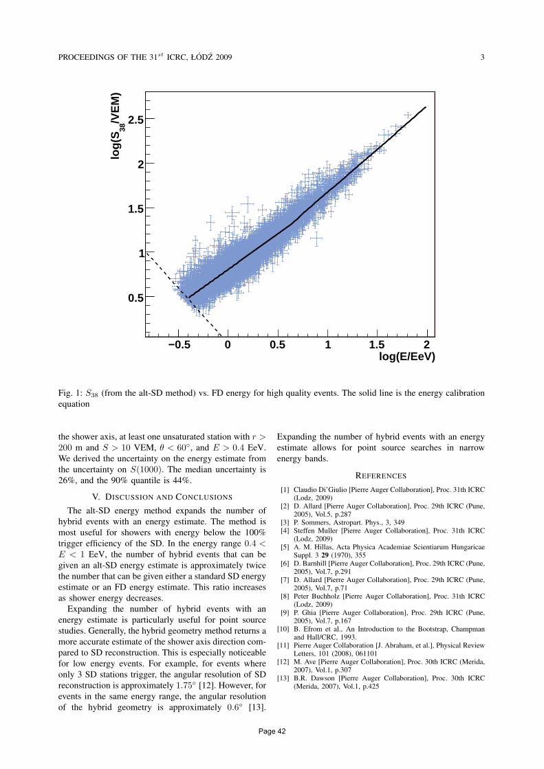
PROCEEDINGS OF THE 31st ICRC, ŁODZ 2009 3
log(E/EeV)−0.5 0 0.5 1 1.5 2
/VE
M)
38lo
g(S
0.5
1
1.5
2
2.5
Fig. 1: S38 (from the alt-SD method) vs. FD energy for high quality events. The solid line is the energy calibrationequation
the shower axis, at least one unsaturated station with r >200 m and S > 10 VEM, θ < 60, and E > 0.4 EeV.We derived the uncertainty on the energy estimate fromthe uncertainty on S(1000). The median uncertainty is26%, and the 90% quantile is 44%.
V. DISCUSSION AND CONCLUSIONS
The alt-SD energy method expands the number ofhybrid events with an energy estimate. The method ismost useful for showers with energy below the 100%trigger efficiency of the SD. In the energy range 0.4 <E < 1 EeV, the number of hybrid events that can begiven an alt-SD energy estimate is approximately twicethe number that can be given either a standard SD energyestimate or an FD energy estimate. This ratio increasesas shower energy decreases.
Expanding the number of hybrid events with anenergy estimate is particularly useful for point sourcestudies. Generally, the hybrid geometry method returns amore accurate estimate of the shower axis direction com-pared to SD reconstruction. This is especially noticeablefor low energy events. For example, for events whereonly 3 SD stations trigger, the angular resolution of SDreconstruction is approximately 1.75 [12]. However, forevents in the same energy range, the angular resolutionof the hybrid geometry is approximately 0.6 [13].
Expanding the number of hybrid events with an energyestimate allows for point source searches in narrowenergy bands.
REFERENCES
[1] Claudio Di’Giulio [Pierre Auger Collaboration], Proc. 31th ICRC(Lodz, 2009)
[2] D. Allard [Pierre Auger Collaboration], Proc. 29th ICRC (Pune,2005), Vol.5, p.287
[3] P. Sommers, Astropart. Phys., 3, 349[4] Steffen Muller [Pierre Auger Collaboration], Proc. 31th ICRC
(Lodz, 2009)[5] A. M. Hillas, Acta Physica Academiae Scientiarum Hungaricae
Suppl. 3 29 (1970), 355[6] D. Barnhill [Pierre Auger Collaboration], Proc. 29th ICRC (Pune,
2005), Vol.7, p.291[7] D. Allard [Pierre Auger Collaboration], Proc. 29th ICRC (Pune,
2005), Vol.7, p.71[8] Peter Buchholz [Pierre Auger Collaboration], Proc. 31th ICRC
(Lodz, 2009)[9] P. Ghia [Pierre Auger Collaboration], Proc. 29th ICRC (Pune,
2005), Vol.7, p.167[10] B. Efrom et al., An Introduction to the Bootstrap, Champman
and Hall/CRC, 1993.[11] Pierre Auger Collaboration [J. Abraham, et al.], Physical Review
Letters, 101 (2008), 061101[12] M. Ave [Pierre Auger Collaboration], Proc. 30th ICRC (Merida,
2007), Vol.1, p.307[13] B.R. Dawson [Pierre Auger Collaboration], Proc. 30th ICRC
(Merida, 2007), Vol.1, p.425
Page 42

4 YOUNK, ALTERNATIVE HYBRID ENERGY DETERMINATION
Fractional Energy Difference (2(SD−FD)/(SD+FD))−1 −0.8 −0.6 −0.4 −0.2 0 0.2 0.4 0.6 0.8 1
Num
ber
of E
vent
s
0
20
40
60
80
100
Fig. 2: Fractional difference between the FD and alt-SD energy for hybrid events above 3 EeV. The dotted line isa Gaussian with a standard deviation of 21%
Page 43
Acknowledgements
The successful installation and commissioning of the Pierre Auger Observatory would nothave been possible without the strong commitment and effort from the technical and admin-istrative staff in Malargue.
We are very grateful to the following agencies and organizations for financial support:
Comision Nacional de Energıa Atomica, Fundacion Antorchas, Gobierno De La Provinciade Mendoza, Municipalidad de Malargue, NDM Holdings and Valle Las Lenas, in gratitudefor their continuing cooperation over land access, Argentina; the Australian ResearchCouncil; Conselho Nacional de Desenvolvimento Cientıfico e Tecnologico (CNPq),Financiadora de Estudos e Projetos (FINEP), Fundacao de Amparo a Pesquisa do Estadode Rio de Janeiro (FAPERJ), Fundacao de Amparo a Pesquisa do Estado de Sao Paulo(FAPESP), Ministerio de Ciencia e Tecnologia (MCT), Brazil; AVCR AV0Z10100502 andAV0Z10100522, GAAV KJB300100801 and KJB100100904, MSMT-CR LA08016, LC527,1M06002, and MSM0021620859, Czech Republic; Centre de Calcul IN2P3/CNRS, CentreNational de la Recherche Scientifique (CNRS), Conseil Regional Ile-de-France,Departement Physique Nucleaire et Corpusculaire (PNC-IN2P3/CNRS), DepartementSciences de l’Univers (SDU-INSU/CNRS), France; Bundesministerium fur Bildung undForschung (BMBF), Deutsche Forschungsgemeinschaft (DFG), FinanzministeriumBaden-Wurttemberg, Helmholtz-Gemeinschaft Deutscher Forschungszentren (HGF),Ministerium fur Wissenschaft und Forschung, Nordrhein-Westfalen, Ministerium furWissenschaft, Forschung und Kunst, Baden-Wurttemberg, Germany; Istituto Nazionale diFisica Nucleare (INFN), Ministero dell’Istruzione, dell’Universita e della Ricerca (MIUR),Italy; Consejo Nacional de Ciencia y Tecnologıa (CONACYT), Mexico; Ministerie vanOnderwijs, Cultuur en Wetenschap, Nederlandse Organisatie voor WetenschappelijkOnderzoek (NWO), Stichting voor Fundamenteel Onderzoek der Materie (FOM),Netherlands; Ministry of Science and Higher Education, Grant Nos. 1 P03 D 014 30, N202090 31/0623, and PAP/218/2006, Poland; Fundacao para a Ciencia e a Tecnologia,Portugal; Ministry for Higher Education, Science, and Technology, Slovenian ResearchAgency, Slovenia; Comunidad de Madrid, Consejerıa de Educacion de la Comunidad deCastilla La Mancha, FEDER funds, Ministerio de Ciencia e Innovacion, Xunta de Galicia,Spain; Science and Technology Facilities Council, United Kingdom; Department of Energy,Contract No. DE-AC02-07CH11359, National Science Foundation, Grant No. 0450696,The Grainger Foundation USA; ALFA-EC / HELEN, European Union 6th FrameworkProgram, Grant No. MEIF-CT-2005-025057, European Union 7th Framework Program,Grant No. PIEF-GA-2008-220240, and UNESCO.
Page 44