ASTROPHYSICAL APL - DIAMONDS IN THE SKY

Glenn Schneider Paul Paluzzi Computer Sciences Corporation Computer Sciences Corporation

Space Telescope Science Institute GreenTec Il 3700 San Martin Drive 10110 Aerospace Road Baltimore, MD 21218 Lanham-Seabrook, MD 20706

James Webb Department of Physics

Stephen F. Austin State University P. 0. Box 13044, SFA Station

Nacogdoches, TX 75962

ABSTRACT

Computational astrophysics seeks to develop numerical models whidh help elucidate the nature of astronomical systems. Such models must not only adequately describe the underlying physics which give rise to phenomena that have been observed, but must also be predictive in asserting what future observations might unfold. Any model which is in conflict with physical observations, clearly, must be discarded or amended to reflect reality. As a computational modelling tool we find /tPL useful for testing astrophysical hypotheses, and extending the domain of our observationally based knowledge. Ltsing APL to build, test, and expand astrophysical models frees the investigator from the mechanical drudgery of computer programming, thereby allowing the researcher to concenuate on understanding the physical universe.

As a quantitative example of how relatively complex astrophysical phenomena can be explored with ease using APL, we have developed a structure model for white dwarf stars. The model presented here considers such effects as Coulomb interactions between electrons and nucleons. inverse beta decays, and the effects of the general theory of relativity on the condition of hydrostatic equilibrium. This structure model is valid for zero-temperature stars of varying chemical compositions, ionic partitions, and central densities; and is applicable ovcx a wide range of partial and total degeneracy regimes.

INTRODUCTION

The quest for understanding the nature, history, and destiny of the physical entities which populate our universe defines the domain of the contemporary astronomer. Gone are the days when the lon,e astronomer would gaze into the heavens for hours on end, peering into a telescope and annotating his or her observations in a bound notebook. The whimsical notion that a telescope “is a long tube with a lens at one end, and an astronomer at the other” (Paul, 1966) has, unfortunately, faded into the historical past. An amendment to this notion, today, would replace the astronomer with an electrooptical detector,

Permksion to cop) without fee all or put of this mat&al is granted prwkkd that the copies are not made or dbkributed for direct commerdal advantage, the ACM copyright ntiice and the title of the publication and its date appear, and notiac is given that copying is by permimion of the Awcciatton for Ccmputtng Mxhtnery. To copy otherwIse, or to republish, requires a fee and/or spedfk pennlsslon. Copyright 1989 ACM o-87971-327-2/ooo8/03rJ4 $1.50

Astrophysical APL - Diamonds in the Sky 304

invariably controlled and read out by computers. Despite popular stereotypes, and romantic notions about the stargazers, contemporary astronomers spend l-5% of their time tending telescopes, and 9599% of their time pushing pencils and pounding on keyboards. The ubiquitous computer has muscled into the astronomers realm and has become as, if not more, important an astronomical tool than the high quality eyepiece at the “astronomers’ end” of the proverbial telescope. Astronomers today compete not only for telescope time, but for computer resources as well, particularly as the power of the new generation of supercomputers becomes available through established research networks. Making optimal use of these computational resources has become paramount, which is where APL comes into the picture.

An astronomer that one of us (GS) knows once had a sign on his office door which proclaimed “Today I am” followed by a tiltable arrow which pointed to “an astronomer”, or “a computer programmer”. The poor fellow would spend days wrestling with a computer, as he would code his way in LISP toward building a model to test a hypothesis which attempted to explain the physics behind some of his astronomical observations. This situation continues to exist within a large segment of the astronomical community, though you may fill in “FORTRAN”, “C”, etc., for your choice of linguistical barriers. Creating computer codes is not what astronomy or astrophysics should be about. Computers make wonderful potential resources, but the languages which we choose to make those computers do our bidding are the tools by which those potentials may become realized. Most computer languages abound in artificial syntactical, grammatical, and operational rules and constructs. This excess baggage serves only as an impediment to transforming the statement of a hypothesis in real, physical terms into a computer model which can be executed and tested.

Employing APL, one can cut through the chaff and get to the meat of problem solving. Indeed, the notion that the mere expression of a problem (in APL notation) is its solution, may not be overstating the case. We have found, using APL, that the ability to move quickly and concisely to an executable model, once a physical hypothesis is sufficiently well formed, is accomplished to a degree far in excess of any other conventional computer language. We measure this degree of success not by evaluating the linguistical compactness, or even the executable efficiency of the software, but rather by the resulting scientific productivity. As a computational modelling tool, APL allows us to obtain results and reject or modify our original hypotheses with both ease and swiftness.

APL89

In this paper we will outline the development of an astrophysical model using APL. To illustrate the flexibility and lucidity of the notation, we attempted to identify those conditions which are often stated by APL opponents as being adverse to the creation of an APL model, and then fmding an astrophysically interesting situation for which those conditions applied. In essence, we looked for things which we, and others, have conjectured that APL does not handle well, and forced their incorporation into our model. Specifically, we demanded that the modeling of the physical process under evaluation must be fundamentally iterative in nature, forcing branching and re-execution of the linguistical constructs to be employed. Additionally, since APL naturally handles the manipulation of extensive multidimensional arrays with ease (Metzger, 1981), in an adverse test the data to be processed were to be of low rank (scalars, vectors, and matrices) containing, in general, very small numbers of elements. Since we were testing a numerical model, we felt that the process should inherently have been computationally extensive. Finally, for this illustrative example to be meaningful to a broad spectrum of potential readers, we wished to find a physical situation which was intrinsically interesting, and not too narrowly channeled. To the latter point, the techniques used in the model would have to be routinely used in diverse astronomical and physical disciplines.

We felt that the classical problem of developing a stellar structure model for white dwarf stars fit all of the above criteria. The numerical integrations of the structure equations from the center of the star to the surface are inherently iterative and computationally intensive. Yet, the physical situation is parametrized by only a few variables, and the number of numerical elements involved in each iteration step is small. In developing the APL model, the method of approach to the solution is as important as, and indeed is part of, the solution itself. The actual “code” (a term we use hesitantly) is developed in a bottom-up fashion, following the structuring of the physical principles employed in the model. There is nothing unique, ground breaking, or particularly inventive in the implementation of the model which we present. The underlying physics is well understood. Indeed, this was an additional requirement we imposed upon ourselves in selecting a situation to model for illustrative purposes.

STRUCTURE MODELS - GENERAL CONCEPTS

For the purposes of developing a model of a stellar interior, the star may be thought of as being comprised of many infintesmally thin, spherically concentric shells. A structure model seeks to determine how the physical properties of the star change at varying depths within the interior. This amounts to determining the “run of physical variables” from the center of the star to the surface (or vice-versa), through each of the spherical shells. Some of the physical variables which are of interest include pressure and density at varying depths (i.e., within each shell), and the mass interior to each shell.

The process of solving the interior model involves expressing the physical relationships between the structure variables as functions of the radial distance from the center of the star, and then determining the numerical values of each of those variables throughout the interior. The form of the classical differential equations of stellar structure, as described by

Schwarzschild (1958), are discussed here as a background to developing the APL model which we will present.

In the interior of a star two forces are in constant competition. The inward acting force of gravity, due to the star’s own mass, seeks to pull the outer layers of the star downward. The internal pressure of the gas, which comprises the stellar material, acts to check this gravitational collapse. For the vast majority of a star’s life these two forces are in balance and the star remains stable. This condition of hydrostatic equilibrium is expressed, for a region in the stellar interior, by equation [ 11.

dPldr = -Gmrp ,/r* 111

The pressure gradient (d Prldr ) across the region

spherical shell) in hydrostatic equilibrium depends upon:

r = the radial distance from the center of the star

mr = the total mass interior to the region

pr = the density of the region

(i.e.,

The distribution of mass as a function of the radial distance from the center of the star is expressed by the equation of mass contirmity, written in differential form in equation [2]. As can be seen, the differential equations of hydrostatic equilibrium and mass continuity both require a knowledge of the density of the region before they can be integrated.

dmjdr = 4m-* p, VI

The gas pressure is related to the temperature and density through an equation of state. The form of the equation of state depends upon the underlying physics which governs the behavior of the gas. The “perfect gas law”, which most of us learned in high school chemistry, comes quite close to reality in physical situations of relatively low gas density, such as in the Earth’s atmosphere and for most of the interior regions of main sequence stars. The perfect gas law assumes that the collisional statistics between the particles in the gas are strictly Maxwellian; all collisions are perfectly elastic, and both external and inter-particle forces (such as Van der Walls forces) are ignored (Sears, 1952). Under higher gas density, as occur in the case of white dwarf stars, such simple assumptions’ will not suffice.

The third equation which describes the structure of the stellar interior is the luminosity gradient equation, expressed in the most general form in equation [3]. This equation states that the radially directed luminosity gradient (i.e., the the net energy loss), across the region is exactly compensated for by the energy generated within the region. The energy generated per unit mass, E, must include all energy sources. For main sequence stars only nuclear energy sources are important, During the pre-main sequence phases of stellar evolution, when the star is undergoing gravitational contraction, both thermal and gravitational energy must also be considered.

dLrldr = Edmjdr [31

Equation [4], which has two forms, describes the radial temperature gradient (d Tr/d r ) across a spherical shell in the

stellar interior.

APL QUOTE QUAD Schneider, Paluui and Webb

d Tidr = [-3KLrp/16nacr2 ~,3]~~~ PaI

d T/dr = [ (1 -Y-l) (frlPJ dq/d rlconv [4bl

The appropriate form of equation [4] to use in the.region depends upon whether the mode of energy transport is radiative or convective. To determine this, the convective form of [4] may be cast as an inequality (Chandrasekhar, 1967). If the region is to be stable against adiabatic convection, then the magnitude of the temperature gradient (d T,/di) must be less than the magnitude of adiabatic temperature gradient. Here,

K = the opacity of the region

a = the Stephan-Boltzman constant C = the speed of light y = the ratio of specific heats of the gas

(513 for highly ionized gas)

White dwarf stars are essentially isothermal. Since there is no physical mechanism for energy generation within the interior, the thermal energy containedthere is a remnant of the core collapse. This remnant thermal energy is bottled up within the star since white dwarfs have small surface areas (typically, less than 10e6 that of the sun). Additionally, a very thin radiative region must exist at the surface. At the interior/surface interface the temperature gradient is large, since the internal temperatures of newly formed white dwarfs are on the order of a few million degrees, while the surface temperatures are observed to be a few times lo4 K. Given a small thin radiative surface area, with a large temperature gradient, white dwarf stars have very long thermal cooling times. Therefore, except for this very thin region at the surface, the temperature gradient in the interior is essentially zero. For these reasons white dwarfs are considered thermally cold, and d Tr ldr in the interior is 0.

As is apparent, the differential equations of stellar structure, [l] - [4], are ~nutually dependent and must be simultaneously integrated to determine the run of the physical variables. The boundary values for the integrations must come from an understanding of the physical properties at the stellar surface and/or center.

Since both the luminosity and thermal gradients (equations [3] and [4]) are zero throughout the interiors of the white dwarfs, the physical characteristics of the interiors of these stars may be inferred only from the differential equations of hydrostatic equilibrium and mass continuity. Hence, we must simultaneously integrate only the first two of the four differential equations of stellar structure.

THE CASE FOR WHITE DWARF STARS

Several complications arise due to the high particle densities which occur in the interiors of white dwarfs. The gas does not behave in accordance with the “perfect gas law”, and indeed is degenerate. In a degent,ate gas both the momenta and the

A star spends most of its life creating energy by nuclear fusion deep in its interior, converting Hydrogen to Helium through the “proton-proton” or “C-N-O” cycles. More massive, evolved stars may also fuse heavier elements, such as Helium into Carbon via the “triple alpha” process. In either case the energy generated in the core provides a sufficient radiant energy flow to support the weight of the outer lying layers, as expressed by the equation of hydrostatic equilibrium. At some point in the life cycle of a star, the available nuclear fuel in the core will be expended. The condition of hydrostatic equilibrium will be violated and the star will collapse under its own gravitational force. The final configuration which will be reached at the end of this rapid collapse depends upon the mass of the star. In any case the outer envelope of the star will be expelled (perhaps violently) or eventually depleted. The remnant stellar core, internally heated and compressed to very high densities by the stellar collapse, is all that will remain of what once was a main sequence star. The compressed core material, often nearly pure Carbon for stars of the appropriate initial mass, is crystalized during the collapse making some white dwarfs truly diamonds in the sky.

positions of the particles are constrained.

The Pauli exclusion principle dictates that no two electrons can have the same position, momentum and spin. The Heisenberg uncertainty principle states that one cannot, even in principle, determine the position and momentum of a particle simultaneously. The location of the particle may be described by its coordinates in a six dimensional phase space; the coordinates being the orthogonal components of the position and momentum vectors. This phase space, conceptually, is comprised of individual cells (whose sides represent conjugate variable pairs in position and momentum, and whose volume is h 3). As the gas density increases, the phase space cells begin to fill up, with the lowest momentum cells being occupied first. Since each cell can hold only two electrons, the distribution function becomes constrained, and is no longer Maxwellian. Such a gas is said to be partially degenerate.

White dwarf stars have peculiar physical properties which in some ways greatly simplifies developing numerical models of their interiors, and in other ways complicates matters enormously. First, simplicity.

In this case, the particle number density and pressure can be derived utilizing Fermi-Dirac statistics. The equation of state (for a given atomic species) may then be characterized by a single parameter representing the energy of the most energetic particle found in the Fermi-Dirac distribution. This parameter, X, is referred to as the “relativity parameter”, and is related to the particle momentum by the usual relativistic relation:

White dwarfs represent the final stage of evolution for many stars. As nokd, at this phase in a star’s life nuclear energy generation processes in the interior have terminated, as the fusionable material has been exhausted. Further, the star is once again in hydrostatic equilibrium, so there is no thermal energy generation to speak of. Therefore, the luminosity gradient, expressed in equation [3] is 0, since E is 0.

x = po/mc [51

where p. is the particle momentum.

The density is related to the relativity parameter, X, through equation [ 61.

p = pMu(xmec/fi)3/37c2 [61

Astrophysical APL - Diamonds in the Sky 306 APL89

where,

P = the ratio of atomic mass to nuclear charge

MU = one atomic mass unit (i.e. 1.6604x10-% gm)

C = the speed of light

me = the mass of an electron

When the phase space cells are completely filled the gas is said to be totally degenerate. At this point no additional particles can be added to the phase space without violating the Pauli exclusion principle. If the pressure exerted on the totally degenerate gas were to be increased further, say by the application of a stronger gravitational field, inverse P-decay would set in. In this process, an electron with “no place to go” (in phase space) would be driven into a proton and combine to form a neutron. This combination event is accompanied by a tremendous energy release, and, if unchecked in the core of a star, results in the onset of a supernova collapse. As we will see, this sets a limiting mass, the Chandrasekhar limit, for white dwarf stars.

In the model we present here we.have chosen the equation of state (EOS) of a degenerate gas developed by Salpeter (1961, p. 669). This EOS incorporates corrections for Coulomb interactions between nucleons and electrons, and both correlation and exchange energy terms. In addition, this EOS considers Thomas-Fermi excess charge distribution effects which become important at high densities where the process of inverse p-decay contributes to the ionic characteristics of the degenerate gas, as discussed by Hamada and Salpeter (1961. p. 683).

Another complication arises from the gravitational field of a white dwarf being so strong that the effects of the general theory of relativity (GTR) cannot be ignored. Here, we are not talking about a further modification of the equation of state, but rather to the structure equations themselves. For the case of hydrostatic equilibrium, Zeldovich and Novikov (1971) solved the metric for the gravitational field of a spherically symmetric star. By integrating the Einstein field equations, the GTR formulation of the hydrostatic equilibrium condition becomes:

-G(pr+Pic2) (mr+4nPrr3/c2)

dPrldr = r2( 1 -2Gmjrc2)

[71

The form of the equation of mass continuity, [2], remains unchanged in the GTR consideration. However, /?7, here is the

total mass-energy of the interior region. At large radii, where the GTR effects are negligible, this reduces to the total stellar mass. We also note that here the radius, f, is that of an equivalent Newtonian sphere, as r, in principle, is unmeasurable under GTR.

AN APL MODEL FOR WHITE DWARF STARS

Armed with an understanding of the basic physics of white dwarf stars, we can now proceed to develop a numerical structure model using APL.

The basic structure of the star is determined by the equations of mass continuity (equation [2]) and hydrostatic equilibrium under GTR (equation [7]). The APL function DES embodies these two differential equations of stellar structure, which must be simultaneously integrated to determine the nm of physical variables throughout the interior of the star.

OD+DES P;S Cl1 0Relatiuistic Strut ture Equations C23 x+(PCll+u)*+3 0 Relativity Parameter C31 qcux(‘EOS z’NEWTON np,x,3LP)t3 FI Dens. t41 Dc4xo (ScPC23t2) xq FI Mass Continuity C51 r+(l+PC43+cxq,+04xPC2 31+.*3 1),+1-2x

+/g,c ,PC3 23 C61 D+D,-gxPC3l+Ssqxx/r ft HS Equilibrium

v

DES[2] and DES[3] compute the numerical values of the relativity parameter, X, and the paricle density, p (called q in DES), which are described by equations [5] and [6], respecitively. DES[4] is the differential of the equation of mass continuity. The three relativistic correction factors, embedded in equation [7], are computed as dimensionless quantities in DES[S] and stored in the vector, r. DES[6] expresses the GTR realization of the equation of hydrostatic equilibrium. Four parameters are passed to ‘DES as a four element vector. The elements of this argument, P, are:

P[l] = the gas density at the lower boundary

P[2] = the distance from the center of the star to the lower boundary

P[3] = the total stellar maSs interior to the lower boundary

P[4] = the gas pressure at the lower boundary

The numerical evaluation of the mass continuity equation requires the determination of density of the degenerate gas at the point of evaluation. This density may be obtained by inverting the Hamada-Salpeter equation of state, described by the function EOS.

OR+X EOS Z;P;AjWjBjE;LjT Cl1 Aiamada-Salpeter Equation of State C21 P+-5.4777336E20 1.50286882E18

+.x(2X2 4+31x(X*4 5)+l,E+40X C 31 L+eB+X+E C41 A+( (B+.tS -5~1 13)+.+32 4)+(1,5xLt2)

-0.5626+ (B- .t2 -2) x3+4+L C51 W+A-X+3+(1+X+E)x(+8+B-.t3 -5)

+ CL+ .x3 -1,5+B,+B+Bt-31-+4+B-Bt-3 C61 Tc8.3656909E20 2.6509094El7+.xW,Xt3 C71 R+P+(6.0025406E22~(3~‘50X)+XxE

x-3+2xX*2 1 -T 0

EOS determines the degenerate gas pressure as a function of the relativity parameter, X, for an atomic species of mass Z. EOS, however, is not analytically invertable. Therefore, a Newton- Raphson iteration scheme is employed to determine the gas density.

APL QUOTE QUAD 307 Schneider, Paluui and Webb

vD+A NEWTON P;T Cl3 nNewton-Raphson Inversion C21 A0:T+&‘PC41’ ,A C33 D~PC~I-(T-~~P)XPC~I+(+‘(+/P~~ 4l)‘,Al-T C41 +BxtPC23>IPC41-D C51 + (xPC33+PE31-ll~A0,PC4l+D C61 D+‘*:ttNO CONVERGENCE: ‘,TPC41-D

0

The Newton-Raphson inversion is performed by the APL function NEWTON. NEWTON is a general routine which may be used to munerically invert any equation expressed as a dyadic APL function. The left argument of NEWTON names the APL function to be inverted, and its invarient right argument (which could. be null), in this case ‘EOS z’. The right argument of NEWTON, P, is a four element vector defined as follows:

P[l] = the value of the differential to be applied in computing numerical derivatives

P[2] = the convergence criterion (numerical precision of the solution)

P[3] = the maximum number of iterations before aborting t’he inversion due to non convergence

P[4] = the value of the functional argument, (x), at the point of inversion

The simultaneous integration of the structure equations, expressed in DES, is handled by the APL function RUNGKUT. As implied by the name, this is an implementation of a Runge- Kutta integration procedure. The algorithm employed for simultaneously integrating the two first order differential equations was described by Scarborough (1966). The left argument of IRUNGKUT is the size of the integration step. The right argument of RUNGKUT are the values of the physical variables (density, radius, interior mass, and pressure, respectively) at the lower boundary of the region to be integrated.

OF+D RUNGKUT F;Kl;K2;K3;K4;A;r;q;x Cl1 RRunge-Kutta Integration C21 Ll :A+‘-4?,F t31 Kl+DxDES A C41 K2cDxDES A+0,0.5xD,Kl C51 K3+DxDES A+0,0.5xD,K2 C61 K4+DxDES A+B,D,KB C71 A+A+(q-ltA),D,+6+1 2 2 1

+.x4 2pKl,K2,K3,K4 C81 F+F,Cllr,x,A c91 +LlxB^.JA

v

Normally, one is only interested in the final result of the integration process. However, the values of the physical variables determined at each integration step of RUNGKUT define the l?yered structure of the star. Therefore, RUNGKUT not only returns the values of the physical variables at the outer boundary of the integration, but the values at each integration step from the lower boundary outward as well. The outer boundary crossing is recognized when the computed value of any of the structure variables becomes negative (as determined in RUNGKUT[9]). Physically, this represents stepping out of the interior of the star, and exiting through the

surface layer. Because of numerical roundoff error (eg., due to the expressed degree of precision in the inversion of EOS by NEWTON) the pressure and the density will not necessarily become negative at the same integration step. As will be seen, both the pressure and the density fall off asymptotically as the stellar surface is approached, so this numerical “fuzz” has little effect on the physical model.

In addition to the structure variables, the relativity parameter, X, and the relativistic correction factors, r, computed by DES at each integration step are accumulated in RUNGKUT[8] and passed in the final result. RUNGKUT returns an eight column matrix, each row containing the values of X, r, p, , r, mr ,

and P,.

The dyadic function WHITEDWARF controls the numerical modelling process.

-R+E WHITEDWARF M;z;np;u;g;c;U Cl1 &tructure Model for White Dwarf Stars C21 cc8.98754E20 ~1 Speed of Light Squared C31 g+6.6732E-8 FI Gravitational Constant C41 z+l?M fi Species Atomic Mass t51 u+973800xMt31 ~1 Partition Function C61 np+lBb-6 -5 2 FI Conuergance, 0, riter C71 RBoundary conditions at center of star C81 U+-8?MC21,10,(oMC21~4000+3~

((CMC21%)*+3)EOS z)-og+200+3+MC2lt2 C93 R+; 8p’J FI Strut ture Matrix ElBl&enter to Surface Integration CllILl:R+-1 0~R,tllMC41RUNGKUT 1 8&J Cl21 U+‘8t,-1 -4tR FI New Boundaries Values Cl31 +(E’MC4l+MC41+10)~Ll

0

The right argument, M, is a four element vector which completely parametrizes the model as indicated below.

M[l] = z,

M121 = pc.

MI31 = PL,

atomic species weight in atomic mass units central density in cgs units

ionic partition function (atomic mass/nuclear charge)

M[4] = Ar, initial value of integration step (dr) in cm.

WHITEDWARF[2]-[6] establishes the values of physical constants used in the model, in cgs units, and sets up the parameters which control the NEWTON inversion routine (the vector np). These, and the value of z, are passed between the functions running under WHlTEDWARF as global variables.

Before the numerical integration can begin, the boundary conditions must be established. The structure model is parametrized by pc, so the density at the center is given. The

approximation can be made that the density at an infinitesimal distance, 5, from the center is the same as it is at the center.

The boundary values for r are computed analytically in WHlTEDWARF[8], as the vector V. In this model we have fixed 5 to a value of 10 cm. The final result of the center-to- surface integration will be passed as the explicit resuh of WHlTEDWARF. WHlTEDWARF[9] establishes a matrix, R, to accumulate this result.

Astrophysical APL - Diamonds in the Sky 308 APL89

The Runge-Kutta integration is invoked by WHlTEDWARF[l l] using the established boundary values. On completion, RUNGKUT will pass the results of its integration from the lower boundary to the surface back to WHITEDWARF. The values in the last row of the matrix passed by RUNGKUT are meaningless, since this corresponds to some small distance outside of the stellar interior. Hence, this row is dropped by WHlTEDWARF[ 121. The structure matrix, then, runs from the lower boundary to as close to the surface as the integration step, Ar, allows without stepping out of the interior. This region, under the surface, can be taken as a new lower boundary, and the integration process may be iterated to get to as close to the surface as desired. WHITEDWARF[13] has been set up to decrease Ar by a factor of 10 when the Runge-Kutta integration is repetitively invoked to closely approach the surface. The left argument of WHITEDWARF, E, specifies the ending value of Ar , for terminating the white dwarf model.

The APL realization of this physical model is short, concise, and easily understood. The question of what represents “good programming style” in APL has been discussed almost endlessly in the literature. The argument has been made that some APLers tend to “one-1inerize”. combining unrelated and disjointed thoughts into a single executable line for the sake of creating artificial brevity of expression. Sadly, this is true. Such practices have been perpetrated by well intentioned, but often unthinking APLers, in attempts to win over or impress those unacquainted with APL of its notative compactness. This invariably leads to slanderous, but not always undeserved comments about “those unreadable chicken scratches”, or the inevitable “looks like Greek to me” remarks.

At the other extreme is the notion that APL statements must be broken down into short segments to enhance readability (APL Quote Quad, 1985). This typically involves the arbitrary inclusion of ultimately vestigial linguistic constructs which serve only to cloud the thoughts enveloped in the APL expression of the problem as discussed by Berry and Pesch (1986). “Enhancing” the readability of the code by incorporating unnecessary assignment statements and additional name references is akin to paying an author by the word rather than for his or her words. In the development of large software systems, it is not uncommon for progress to be measured by the number of lines of executable code. Do we really want this sort of outlandish situation in APL?

As a tool of thought a computer language should not impose artificial linguistic or stylistic constraints on the thinker. The thought processes which are implicitly mapped into the code should not be obscured by “enhancement”, either by lengthening or shortening the notative representation of the problem at hand. We believe that as a case in point the white dwarf model presented here illustrates this, and the concept that “APL possesses certain important characteristics which speed development and assist thought” (Bemecky, 1986).

In developing our APL model of white dwarf stars we made no effort to either “one-linerize”, or to break up logically connected thoughts to, as suggested by some, aid’ in the readability of the code. On the contrary, just as each function represents a modular piece of the solution, in a hierarchial sense, each function line represents a discrete “chunk” of thinking.

APL QUOTE QUAD 309

NUMERICAL RESULTS

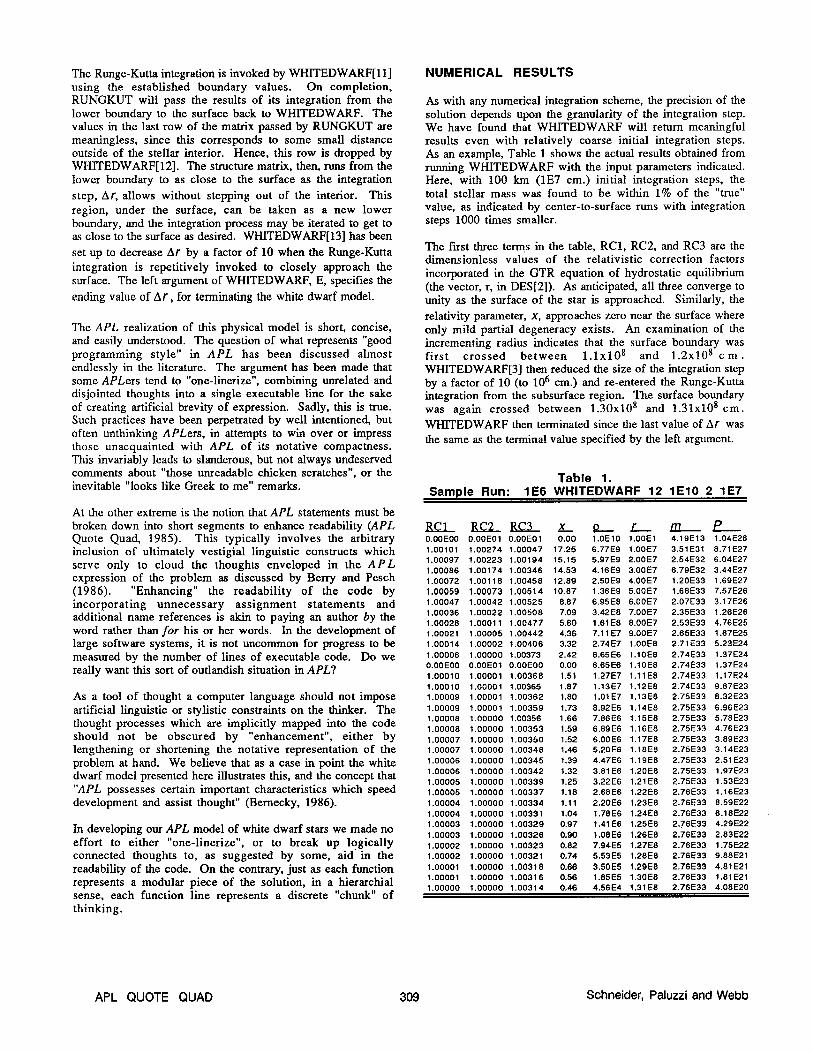
As with any numerical integration scheme, the precision of the solution depends upon the granularity of the integration step. We have found that WHITEDWARF will return meaningful results even with relatively coarse initial integration steps. As an example, Table 1 shows the actual results obtained from running WHITEDWARF with the input parameters indicated. Here, with 100 km (lE7 cm.) initial integration steps, the total stellar mass was found to be within 1% of the “true” value, as indicated by center-to-surface runs with integration steps 1000 times smaller.

The Fist three terms in the table, RCl, RC2, and RC3 are the dimensionless values of the relativistic correction factors incorporated in the GTR equation of hydrostatic equilibrium (the vector, r, in DES[2]). As anticipated, all three converge to unity as the surface of the star is approached. Similarly, the relativity parameter, X, approaches zero near the surface where only mild partial degeneracy exists. An examination of the incrementing radius indicates that the surface boundary was first crossed between 1.1~10~ and 1.2~10~ cm. WHITEDWARF[3] then reduced the size of the integration step by a factor of 10 (to lo6 cm.) and re-entered the Runge-Kutta integration from the subsurface region. The surface boundary was again crossed between 1.30x10* and 1.31~10~ cm. WHITEDWARF then terminated since the last value of Ar was the same as the terminal value specified by the left argument.

Table 1. Sample Run: 1 E6 WHITEDWARF 12 1 El0 2 1 E7

EcLIGLluzLxormP O.OOEOO O.OOEOl O.OOEOl 0.00 l.OElO l.OOEl 4.19E13 1.04E26 1.00101 1.00274 1.00047 17.25 6.77E9 l.OOE7 3SlE31 6.71E27 1.00097 1.00223 1.00194 15.15 5.97E9 2.00E7 2.54E32 6.04E27 1.00066 1 .00174 1.00346 14.53 4.16E9 3.00E7 6.79E32 3.44E27 1.00072 1 .00116 1.00456 12.69 2.50E9 4.00E7 1.20E33 1.69E27 1.00059 1.00073 1.00514 10.67 1.36E9 5.00E7 1.66E33 7.57E26 1.00047 1.00042 1.00525 6.67 6.95E6 6.00E7 2.07E33 3.17E26 1.00036 1.00022 1.00506 7.09 3.42E6 7.00E7 2.35E33 1.26E26 1.00026 1 .OOOl 1 1.00477 5.60 1.61 E6 6.OOE7 2.53E33 4.76E25 1.00021 1.00005 1.00442 4.36 7.11 E7 9.00E7 2.65E33 1.67E25 1 .00014 1.00002 1.00406 3.32 2.74E7 l.OOE6 2.71E33 5.23E24 1.00006 1 .ooooo 1.00373 2.42 6.65E6 l.lOE6 2.74E33 1.37E24

O.OOEOO O.OOEOl O.OOEOO 0.00 6.65E6 l.lOE8 2.74E33 1.37E24 1.00010 1.00001 1.00368 1.51 1.27E7 l.llE6 2.74E33 1.17E24 1 .OOOl 0 1 .OOOO 1 1.00365 1 .a7 1.13E7 1.12E6 2.74E33 9.67E23 1.00009 1 .OOOOl 1.00362 1.60 l.OlE7 1.13E6 2.75E33 6.32E23

1.00009 1.00001 1.00359 1.73 8.92E6 1.14E6 2.75E33 6.96E23 1.00006 1 .OOOOO 1.00356 1.66 7.66E6 1.15E6 2.75E33 5.76E23 1.00006 1.00000 1.00353 1.59 6.69E6 1.16E6 2.75E33 4.76E23 1.00007 1 .ooooo 1.00350 1.52 6.00E6 1.17E6 2.75E33 3.69E23 1.00007 1 .ooooo 1.00346 1.46 5.20E6 1.16E6 2.75E33 3.14E23 1.00006 1 .OOOOO 1.00345 1.39 4.47E6 1.19EB 2.75E33 2.51 E23 1.00006 1 .OOOOO 1.00342 1.32 3.61 E6 1.20E6 2.75E33 1.97E23 1.00005 1 .OOOOO 1.00339 1.25 3.22E6 1.21E8 2.75E33 1.53E23 1.00005 1 .ooooo 1.00337 1.16 2.68E6 1.22E8 2.76E33 1.16E23 1.00004 1 .ooooo 1.00334 1.11 2.20E6 1.23E6 2.76E33 6.59E22 1.00004 1 .ooooo 1.00331 1.04 1.78E6 1.24E6 2.76E33 6.16E22 1.00003 1 .OOOOO 1.003?9 0.97 1.41 E6 1.25E6 2.76E33 4.29E22 1.00003 1 .OOOOO 1.00326 0.90 1.08E6 1.26E6 2.76E33 2.63E22 1.00002 1 .OOOOO 1.00323 0.62 7.94E5 1.27E6 2.76E33 1.75E22 1.00002 1 .OOOOO 1.00321 0.74 5.53E5 1.26E6 2.76E33 9.66E21

1.00001 1.00000 1.00318 0.66 3.50E.5 1.29E6 2.76E33 4.61 E21 1 .OOOOl 1 .OOOOO 1.00316 0.56 1.85E5 1.30E6 2.76E33 1.61 E21 1.00000 1.00000 1.00314 0.46 4.56E4 1.31 E6 2.76E33 4.08E20

Schneider, Paluzzi and Webb

By comparing models of white dwarfs of given compositions, one can try to predict how the interior structure and global properties of these stars vary as a function of the principle characterizing parameter - the central density, pc. The final

results obtained for the integrated global structure of eleven Carbon white dwarfs (Z=lZ, l.t=2.00) of increasing central density are summarized in Table 2. This table gives the central density (pc)., total stellar mass (M) and radius (R) of each of the

stars modeled. The first four columns are in cgs units, while the last two columns compare the computed masses and radii of the Carbon white dwarfs to that of the sun (Ma and R 0, respectively). Some rather interesting physical properties of these stars are predicted by these results.

Table 2. Globall Properties of Carbon White Dwarfs

log P, 4 Mx~O-~~ Rx~O-~ M/Ma 1 OOFVb ________ __~.---____ ------------ ---------- ---------- ------------

7.0 8.:21E23 1.540 6.840 0.774 0.983 7.3 2.:22E24 1.785 5.965 0.897 0.857 8 .O 2. LOE25 2.253 4.223 1.132 0.607 8.3 5.39E25 2.397 3.602 1.204 0.518 9 .O 4:?5E26 2.613 2.421 1.313 0.348 9.3 l.:20E27 2.665 2.022 1.339 0.290

10.0 1.04E28 2.727 1.294 1.370 0.186 10.3 2LiOE28 2.736 1.059 1.375 0.152 11 .O 2.:24E29 2.733 0.652 1.374 0.094 11.3 5.152E29 2.723 0.526 1.369 0.076 12.0 482E30 2.682 0.315 1.348 0.045

First, as can be seen, white dwarfs with higher central densities (and correspondingly higher central pressures) contain more mass up to a limit of log pc = 10.3. An increase in total mass

with increasing central density seems almost obvious from physical arguments invoking mass continuity and hydrostatic equilibrium. What is interesting, however, is that the mass does not increase without bound as a function of pc, but

approaches a maximum 2.74~10~~ grams and then begins to decrease. This critical mass, well known as the Chandrasekhar limit, represents the most massive configuration that a white dwarf can obtain before mechanical equilibrium begins to break down and inverse beta decay sets in. In this condition the gas throughout is completely degenerate. If additional mass were suddenly dumped onto the star, the white dwarf could implode forming a neutron star. Chandrasekhar originally predicted the limiting mass for a white dwarf to be 1.44 solar masses. This model predicts 1.38 solar masses as an upper limit. The difference arises when one considers both the effects of general relativity on the condition of hydrostatic equilibrium and the additional gas pressure terms accounted for in the Hamada-Salpeter equation of state..

Second, the radii of white dwarfs decrease with increasing central prelrsure, and correspondingly increasing central density. As illustrated in Figure 1, up to the turnover point of log p, = 10.3, white dwarfs of greater total mass become

physically smaller! This obviously implies increase in the gas density (and pressure) throughout the interior. Theoretically, as the central density is increased, and as Chandraseklnar’s limit is approached, the radius of the star

drops to zero. Clearly, a condition of instability resulting in a physical change in the overall configuration of the star would occur before such a singularity is reached. Indeed, this is precisely the condition which would ultimately lead to the catastrophic formation of a neutron star.

8.7--

’ .A--

e.s-- .A--

e.3-- .A?--

8,1-- logpc lndlc~tdhrcuhcomputed potnt

e.e, 1 : 1 : 8.75 e Al5 8.95 I .es 1.15 1.25 1.35

I n/n,

Figure 1. Mass/Radius Relation for Carbon White Dwarfs

The interior structure of the star, as a function of the distance from the star’s center, may also be inferred from the WHITEDWARF model. For example, Figure 2 shows how the pressure in the interior drops off, from the center of the star to the surface, for Carbon white dwarfs of varying central densities. Both the pressure at a given radius and the radial distance from the center are normalized to the central pressure and radius at the surface, respectively. This allows for easily intercomparing the differences in structure, while recognizing that the actual dimensions of the physical variables change from star to star as reported in Table 2. As is apparent, the pressure gradient is more severe close to the center of those white dwarfs with greater central gas pressures (and correspondingly greater gas densities).

-l l .e e.1 l .2 l .3 e-4 8.5 e.6 l .7 e.e ‘ .e

FRACTIONAL RADIUS (r/R,)

Figure 2. Pressure Gradient in Carbon White Dwarfs

The distribution of mass in Carbon white dwarfs, as predicted in the WHITEDWARF model, is represented in a similar fashion in Figure 3. Here, the fractional mass, m,, is the

fraction of the stars mass contained within the corresponding fractional radius. As is obvious from this figure white dwarf stars with higher central pressures are more centrally condensed.

Astrophysical APL - Diamonds in the Sky APL89

-. -. ---...

3.3 0.1 3.3 6.3 6.4 3.5 6.6 3.7 6.3 3.6 1.3 FRACTIONAL RADIUS (r/R.)

Figure 3. Mass Distribution in Carbon White Dwarfs

It is beyond the intended scope of this paper to consider the physical results in greater detail than we have discussed here. For example, we have elaborated on the interrelation of only a few of the structure parameters. Indeed, our principle intent was to demonstrate the utility of APL for moving rapidly and easily from the physical conception of a given problem to the actualization of a computational model. In particular, while we have only discussed the WHITEDWARF results for pure Carbon white dwarfs, the model inherently will work with other atomic species and ionic partitions. We invite the reader to use the model to build white dwarf stars of his or her l&in

9 (we offer as

suggestions for individual exploration He4, Mg 4, Si2*. S32, and Fes6).

WHITEDWARF serves as a useful tool in its own right in helping to come to an understanding of the structure of white dwarf stars. Yet, WHITEDWARF though rigorous in many ways is idealized in others. The model presented here does not consider such effects as stellar rotation, magnetic fields, mass accretion (in binary systems), and other complicating factors which one can posit. For example, in rotating stars one must consider how the angular momentum of the gas particles contributes to the physical stability of the system (Tassoul. 1978). Since the angular velocity at a given radial distance from the center varies as the cosine of the latitudinal angle measured from the rotational equator, the problem becomes a two dimensional one. Simple spherical symmetry cannot, a priori, be assumed. Moving from a one dimensional model to a two dimensional one in APL is almost trivial; for as is well known, and accepted even by APL opponents, APL shines as an array processing language. We leave this for any interested parties “as an exercise for the reader”.

ACKNOWLEDGEMENTS AND FINAL COMMENTS

We would like to thank Dr. Robert Wilson of the University of Florida’s Department of Astronomy for first suggesting this problem to us. Our gratitude is extended to Andrew Weisenberger of the Space Astronomy Laboratory who was instrumental in the initial formulation of this problem. This model was first implemented on a Commodore SP9000 (SuperPETTM) computer running Waterloo microAPL 1.0 (Wilson and Wilkinson, 1981). illustrating that real science can indeed be done in a 28K workspace. The version of the WHITEDWARF code shown here, and the numerical results, were run on a Macintosh@ SE under MicroAPL Ltd’s

APL QUOTE QUAD 311

APL.68000~ (1986a,b) distributed by the Spencer Orginization. For those readers who have stayed with us to the bitter end we offer the follwing note of explanation:

This paper was not about statement delimitation in APL.’

0

‘We hope the title was not deceiving.’

REFERENCES

APL Quote Quad, APL Quote Quad Style Guide for APL Functions. APL Quote Quad 15 3, 1985.

Berry, Michael and Pesch, Roland, Style and Literacy in APL. APL86 Conference Proceedings (APL Quote Quad 16 4). 1986.

Bemecky. Robert, APL: A Prototyping Language. APL86 Conference Proceedings (APL Quote Quad 16 4), 1986.

Chandrasekar, S., An Introduction to the Study of Stellar Structure. Dover Publications, 1967.

Hamada T. and Salpeter E.E., Models for Zero-Temperature Stars. Astrophysical Journal, 134 3, 1961.

Metzger, Robert C., APL Thinking Finding Array-Oriented Solutions. APL81 Conference Proceedings (APL Quote Quad 12 1). 1981.

MicroAPL, Ltd., APL.68000m Language ManuaL.1986.

MicroAPL, Ltd., APL.68000” for the AppleTM MacintoshTM. 1986.

Paul, Henry E., Telescopes for Skygazing. Sky Publishing Corporation, 1966.

Salpeter, E.E., Energy and Pressure of a Zero-Temperature Plasma. Astrophysical Journal, 134 3, 1961.

Scarborough, James B., Numerical Mathematical Analysis. sixth edition, The Johns Hopkins Press, 1966.

Schwarzschild, Martin, Structure and Evolution of the Stars. Dover Publications, 1958.

Sears, Francis, W, Thermodynamics, The Kinetic Theory of Gases, and Statistical Mechanics. second edition, Addison- Wesley Publishing Company, Inc., 1952.

Tassoul, Jean L., Theory of Rotating Stars. Princeton University Press, 1978.

Wilson, J.C., and Wilkinson, T.A., Waterloo microAPL Tutorial and Reference Manual. 198 1.

Zeldovich Ya. B., and and Novikov. I.D., Relativistic Astrophysics. Volume 1, University of Chicago Press, 1971.

Schneider, Paluui and Webb

. .