Astron. Astrophys. 358, 1–12 (2000) ASTRONOMYAND

ASTROPHYSICS

Space-time distributions of QSO absorption systems

A.D. Kaminker, A.I. Ryabinkov, and D.A. Varshalovich

A.F. Ioffe Physical Technical Institute, Politekhnicheskaya 26, 194021 St.-Petersburg, Russia (kam@astro.ioffe.rssi.ru)

Received 9 August 1999 / Accepted 21 March 2000

Abstract. A statistical analysis of the distributions of C IVand Mg II absorption-line systems observed in quasar spectrawithin the cosmological redshift intervalz = 0.2–3.2 is pre-sented. The results indicate that the overallz-distribution ofabsorbing matter is non-uniform: it has statistically significantmaxima and minima, but it appears statistically isotropic. Themaxima in thez-distribution of absorption systems are found atzm = 0.44, 0.77, 1.04, 1.30, 1.46, 1.60, 1.78, 1.98, 2.14, 2.45,2.64, and 2.86(±0.04). The positions of maxima and minimaof the z-distribution turn out to be the same (within the sta-tistical uncertainty) for different celestial hemispheres indepen-dently of their orientation. The resulting space-time distributionof absorbing matter resembles successively embedded spherescorresponding to thezm values indicated. The most probableorigin of such a distribution is an alternation of pronounced anddepressed epochs in the course of cosmological evolution.

Key words: galaxies: quasars: absorption lines – cosmology:large-scale structure of Universe

1. Introduction

Most cosmological models are based on the cosmological prin-ciple (e.g., Peebles 1993) which assumes that all points of spaceand all directions of observations are equivalent, so that the Uni-verse is, on average, uniform and isotropic. It was reliably con-firmed by the latest observations of Cosmic Microwave Back-ground at the relative level<∼ 10−5 at least up to arc-degreescales. On the other hand, the local distribution of matter sur-rounding our Galaxy is not uniform. Moreover, there exists ahierarchy of scales of galaxy clusters and superclusters in ad-dition to familiar small-scale inhomogeneities of galaxies (e.g.,Bahcall 1995). The largest known inhomogeneities of matterform the so–called Large-Scale Structure (LSS) discovered inthe last decade at moderate redshifts (z <∼ 0.6) (e.g., Broadhurstet al. 1990, Landy et al. 1996, Einasto et al. 1997). It is quiteprobable that the specific scale of the largest inhomogeneitieshas changed noticeably in the course of the cosmological evo-lution. Therefore it is worth while to investigate the uniformity

Send offprint requests to: A.D. Kaminker

and isotropy of the distribution of matter on larger cosmologi-cal space-time scales at higher redshifts. In particular, one canuse available observational data on redshifted absorption-linesystems imprinted on spectra of quasars (QSOs) for a statisticalanalysis of absorbing material at redshiftsz >∼ 1.

The analysis of some line-of-sight spatial correlation func-tion for C IV absorption-line systems in QSO spectra was car-ried out by Quashnock et al. (1996) in the redshift intervalz = 1.2–4.5. They found the clustering of C IV absorbers oncomoving scales comparable with the LSS (see Sect. 4). How-ever, the correlation function they used could not represent com-pletely general properties of thez-distribution of the absorbingmatter.

The degree of uniformity and isotropy of the distributionof C IV absorption systems atz = 1.2–3.2 was analyzed byRyabinkov et al. (1998). Here we present results of an investi-gation of the distribution of absorption matter in a wider red-shift intervalz = 0.2–3.2. We use the absorption lines of theresonance doublets C IV(λ0

1 = 1548 A and λ02 = 1551 A),

and Mg II (λ01 = 2796 A and λ0

2 = 2804 A) as indicators ofabsorbing material existing at the redshifts under study (sub-scripts 1 and 2 numerate lines of doublets, superscript0 denoteslaboratory values). These spectral lines are usually observed inQSO spectra with high emission-line redshiftze. We assumethat the redshift of the absorption linesza is cosmological, i.e.,λ = λ0(1 + za), and the observed absorption-line systems areassociated with ionized gas in intervening galaxies or clusters ofgalaxies at large cosmological distances along the line-of-sightbetween QSO and observer.

Notice that an analysis of thez-distribution of photon meanfree paths based on the statistics of QSO absorption-line sys-tems has been performed recently by Liu & Hu (1998). Using thedata on QSO absorption redshifts from the catalog of Junkkari-nen et al. (1991) they found that the mean free path displaysquasi-periodic component with alternating sharp maxima andminima in addition to the monotonic trend. We will show thatthese results appear to be qualitatively consistent with the resultspresented here, although our observational data and statisticalapproach are rather different.

In Sect. 2 we present statistical evidence for a non-uniform– sequence of significant maxima and minima – but an isotropicdistribution of matter using data on C IV and Mg II absorption

2 A.D. Kaminker et al.: Space-time distributions of QSO absorption systems

systems in the redshift intervalsz = 1.2–3.2 andz = 0.2–2.1,respectively. Similar results obtained by the analysis of the nor-malized distribution which enable us to avoid some of observa-tional selection effects are given in Sect. 3. In Sect. 4 we discusssome effects of possible clustering of the absorbing matter onthe set of maxima and minima revealed. In Sect. 5 we presenttests of possible regularity of the distribution obtained. Conclu-sions and possible consequences of the results are discussed inSect. 6.

2. Analysis of C IV and Mg II absorption systems

2.1. Criteria of sampling

We consider inhomogeneous statistical material since we useavailable data on QSO spectra obtained in different studies,which applied different criteria for line detection and systemidentification. In such a situation, probabilities of registrationof absorption systems could bea priori different for differ-ent values ofz, and this could simulate non-uniformity ofz-distributions. Additional selection effects may be induced by thenon-cosmological movement of absorbing matter in the nearestneighborhood of QSOs and by small-scale clustering of closeabsorption features corresponding to clouds within one galaxy.In order to reduce an influence of all such selection effects oneshould analyse available data using a unified procedure of sam-pling.

Let us start from the determination of criteria and conditionswhich are used in our discussion. We consider the wavelengthintervals in the observed QSO spectra between emission linesC IV and Ly-α as well as Mg II and Ly-α. The boundaries ofthese intervals are determined in terms of their redshiftszi

min ≤za ≤ zi

max, where the indexi = 1, 2, .. covers all observationsof the QSO spectra sampled for the analysis. The valueszi

minandzi

max are set to obey additional conditions:

zimin ≥ 1.5Ri

λ02 − λ0

1− 1;

zimax ≤ ze − ve

c(1 + ze), (1)

whereRi = FWHMi represents the spectral resolution (inA) forthei-th spectral interval, andve = 3000 km s−1 is the velocityshift allowed for the absorption system relative to the corre-sponding emission line. The first condition rejects all unreliabledoublets and the second one eliminates absorption systems withan essential part of their redshifts due to non-cosmological ori-gin, e.g., expansion of QSO envelopes. Thus, only absorbers(intervening galaxies or clusters of galaxies) situated quite farfrom the corresponding QSOs were sampled for our considera-tion. In this way we selectedNQSO = 398 of observed spectralintervals for 250 QSOs.

For eachi-th spectral interval we calculate the thresholdvalue of the absorption equivalent width

W ith =

51 + zi

min

Ri

< S/N >i, (2)

where< S/N >i is the signal-to-noise ratio averaged over thewholei-th interval. An absorption line with an equivalent widthin the rest frameWλ/(1 + za) ≥ W i

th could have been reliablydetected in thei-th interval of the redshifts. We adopt also theequivalent width of the weaker line (λ0

2) of a doublet as theequivalent width of the absorption systemWabs.

In order to reveal possible large scales and suppress smallscales, we take into account only separate absorbers eliminatingthe well-known tendency of the neighbouring absorption sys-tems to cluster on a velocity scale∆v <∼ 600 km s−1 (see, e.g.,Val’tts 1991, Steidel & Sargent 1992, Quashnock et al. 1996).Therefore, we consider any two close systemsz′

a andz′′a situated

along the line of sight as a single one withza = (z′a + z′′

a )/2andWabs = W ′

abs + W ′′abs under the condition

∆v

c=

∆z

1 + za≤ 0.002, (3)

wherec is the speed of light, and∆z = |z′a − z′′

a |.To make the statistics of selected absorption systems more

homogeneous we use two criteria of sampling of observationaldata:detectionand identification. Let us assume thatni ≥ 0absorption systems of C IV or Mg II were registered with red-shiftszij

a and equivalent widths in the rest frameW ijabs, in each

i-th spectral interval, where indexj = 1, 2, ...ni, for ni ≥ 1,numerates all observed systems inside thei-th interval. Thenthe criterion of thedetectionof j-th absorption system is

W ijabs =

(Wabs

1 + za

)ij

≥ W ith, (4)

whereW ith is determined by Eq. (2).

The criterion ofidentificationfor the resonance doublets ofC IV or Mg II consists of two conditions:∣∣∣∣λ2

λ02

− λ1

λ01

∣∣∣∣ ≤ 10−3;

1 ≤ Wλ1

Wλ2≤ 2, (5)

whereWλ1 andWλ2 are the equivalent widths of doublet lineswith account of their uncertainties.

2.2. Uniformity of the distributions

According to the criteria described in Sect. 2.1 we considered299 C IV absorption systems in the redshift intervalz = 1.2–3.2and 216 Mg II absorption systems in the intervalz = 0.2–2.1,observed in QSO spectra (Bergeron et al. 1987; Boisse & Berg-eron 1985; Caulet 1989; Foltz et al. 1986; Khare et al. 1989;Lanzetta et al. 1987; Lanzetta & Bowen 1992; Petitjean & Berg-eron 1990; Robertson et al. 1986, 1988; Sargent et al. 1982,1988a, 1988b, 1989, 1990; Sargent & Steidel 1987; Steidel1990; Steidel & Sargent 1992; Turnshek et al. 1989; Younget al. 1982).

Our starting hypothesis (null-hypothesis) is the assumptionof uniform distributions of the samples relative to linear func-tions (trends)Ntr = a + bz, obtained in the redshift intervals

A.D. Kaminker et al.: Space-time distributions of QSO absorption systems 3

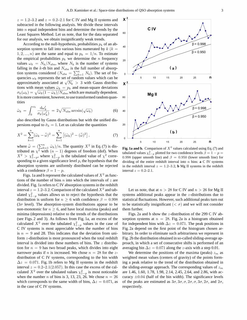
z = 1.2–3.2 andz = 0.2–2.1 for C IV and Mg II systems andsubtracted in the following analysis. We divide these intervalsinto n equal independent bins and determine the trends by theLeast Squares Method. Let us note, that for the data separatedfor our analysis, we obtain insignificantly weak trends.

According to the null-hypothesis, probabilitiespk of an ab-sorption system to fall into various bins numerated byk (k =1, 2, ..., n) are the same and equal topk = 1/n. To estimatethe empirical probabilitiespk we determine then frequencyvaluesωk = Nk/Nabs, whereNk is the number of systemsfalling in the k-th bin andNabs is the full number of absorp-tion systems considered(Nabs =

∑nk=1 Nk). The set of fre-

quenciesωk represents the set of random values which can beapproximately associated at

√Nk > 3 with Gauss distribu-

tions with mean valuesωk = pk and mean-square deviationsσk(ωk) =

√ωk(1 − ωk)/Nabs, which are mutually dependent.

It is more convenient, however, to use transformed random quan-tities

ωk =∫ ωk

0

dω′k

σk(ω′k)

= 2√

Nabs arcsin(√

ωk) (6)

also described by Gauss distributions but with the unified dis-persions equal toσk = 1. Let us calculate the quantities

X2 =n∑

k=1

(ωk − ¯ω)2 =n∑

k=1

[(ωk)2 − (¯ω)2

], (7)

where ¯ω = (∑n

k=1 ωk)/n. The quantityX2 in Eq. (7) is dis-tributed asχ2 with (n − 1) degrees of freedom (dof). WhenX2 > χ2

1−p, whereχ21−p is the tabulated value ofχ2 corre-

sponding to a given significance levelp, the hypothesis that theabsorption systems are uniformly distributed can be rejectedwith a confidenceβ = 1 − p.

Figs. 1a and b represent the calculated values ofX2 as func-tions of the number of binsn into which the intervals ofz aredivided. Fig. 1a refers to C IV absorption systems in the redshiftintervalz = 1.2–3.2. Comparison of the calculatedX2 and tab-ulatedχ2

1−p values allows us to reject the hypothesis that thedistribution is uniform forn ≥ 6 with confidenceβ = 0.998(3σ level). The absorption-system distributions appear to benon-monotonic forn ≥ 6, and have local maxima (peaks) andminima (depressions) relative to the trends of the distributions(see Figs. 2 and 3). As follows from Fig. 1a, an excess of thecalculatedX2 over the tabulatedχ2

1−p values in the case ofC IV systems is most appreciable when the number of binsis n = 9 and 28. This indicates that the deviation from uni-form z-distribution is most pronounced when the total redshiftinterval is divided into these numbers of bins. Thez distribu-tion for n = 9 has two broad peaks, which divides into eightnarrower peaks ifn is increased. We chosen = 28 for thez-distribution of C IV systems, corresponding to the bin width∆z = 0.071. Fig. 1b refers to Mg II systems in the redshiftintervalz = 0.2–2.1(2.057). In this case the excess of the cal-culatedX2 over the tabulated valuesχ2

1−p is most noticeablewhen the numbern of bins is 3, 13, 23, 26. We chosen = 26which corresponds to the same width of bins,∆z = 0.071, asin the case of C IV systems.

&,9

β

β

;

Q

D

0J,,

β

β

;

Q

E

Fig. 1a and b. Comparison ofX2 values calculated using Eq. (7) andtabulated valuesχ2

1−p plotted for two confidence levelsβ = 1 − p =0.998 (upper smooth line) andβ = 0.950 (lower smooth line) fordividing of the entire redshift interval inton bins: a C IV systemsin the redshift intervalz = 1.2–3.2, b Mg II systems in the redshiftintervalz = 0.2–2.1.

Let us note, that atn > 28 for C IV andn > 26 for Mg IIsystems additional peaks appear in thez-distributions due tostatistical fluctuations. However, such additional peaks turn outto be statistically insignificant(< σ) and we will not considerthem further.

Figs. 2a and b show thez-distribution of the 299 C IV ab-sorption systems atn = 28. Fig. 2a is a histogram obtainedfor independent bins with∆z = 0.071. The peak positions inFig. 2a depend on the first point of the histogram chosen ar-bitrary. In order to eliminate such arbitrariness we represent inFig. 2b the distribution obtained in so-called sliding-average ap-proach, in which a set of consecutive shifts is performed of anaveraging bin∆z = 0.071 along thez-axis with a step 0.01.

We determine the positions of the maxima (peaks)zm asweighted mean values (centers of gravity) of the points form-ing a peak relative to the trend of the distribution obtained inthe sliding-average approach. The corresponding values ofzm

are 1.46, 1.60, 1.78, 1.98, 2.14, 2.45, 2.64, and 2.86, with ac-curacy±0.04 (half of the bin width). The significance levelsof the peaks are estimated as3σ, 3σ, σ, 2σ, σ, 3σ, 2σ, and2σ,respectively.

4 A.D. Kaminker et al.: Space-time distributions of QSO absorption systems

1N

=

&,9 D

1N

=

E

Fig. 2a and b. z-distribution of 299 absorption systems of C IV:a his-togram with bin size∆z = 0.071, b sliding-average distribution withaveraging bin0.071 and step0.01 (see text for details).

The results for Mg II absorption-line systems are quite con-sistent with the results discussed above. Figs. 3a and b showthez distribution of 216 Mg II absorption systems forn = 26.Fig. 3a is the histogram obtained for independent bins with thesame width∆z = 0.071 as in Fig. 2a. Fig. 3b shows the distri-bution obtained in the sliding-average approach. The values ofthe centers of gravity of the peaks are equalzm = 0.44, 0.77,1.04, 1.30, 1.66, and 1.78(±0.04). The significance values ofthe peaks are2σ, σ, 3σ, 4σ, σ, andσ, respectively. One can see,that the last two peaks of Mg II systems are in a good agree-ment with the second and third peaks in the distribution of C IVsystems. However, the first conspicuous peak atzm = 1.46 inthez-distribution of C IV systems is not seen in Fig. 3.

Thus, our results concerning both C IV and Mg II absorptionsystems provide evidence for non-uniform distribution of matterin the redshift intervalz = 0.2–3.2 at a confidence level higherthan0.998.

2.3. Isotropy of the distributions

We test isotropy (or anisotropy) of distributions by compar-ing thez-distributions of C IV and (separately) Mg II systemsin opposite independent hemispheres. For this purpose we di-vide the celestial sphere (Equatorial coordinates) into two hemi-

1N

0J,,

=

D

1N

=

E

Fig. 3a and b. Same as Fig. 2, but for 216 absorption systems of Mg II.

spheres separated by the plane passing through the world axis(δ = ±90, δ is a declination) and rotate this plane about theworld axis by steps∆α = 15(1h), whereα is a right ascension.In such a way we obtain 12 pairs of independent hemispheres.For each hemisphere, we obtain thez-distribution of the ab-sorption systems, the linear trends (see Sect. 2.2) having beenexcluded in all hemispheres. Let us note that dividing the celes-tial sphere into smaller parts leads to an increase of statisticalerrors. We calculate the correlation coefficientr for each pair ofindependent hemispheres and compare it with tabulated valuesrβ of the sample correlation coefficient for a given sample sizen and the confidence levelβ (dof= n − 2).

Fig. 4 shows thez-distributions in two opposite hemispheresα = 0–180 andα′ = 180–360. The calculated correlationcoefficient for these two distributions isr = 0.670, while rβ =0.588 for n = 28 andβ = 0.999; this provides evidence thatthe two distributions obtained are correlated better than at the3σ level.

Fig. 5a represents the correlation coefficients for thez-distributions in pairs of opposite hemispheres as a function ofthe right ascensions of the centers of the hemispheres for twocomplementary intervals0 ≤ αc ≤ 180 (lower horizontalaxis) and180 ≤ α′

c ≤ 360 (upper horizontal axis). It is clearthat the correlation of thez-distributions is significant, as a rule,at the2σ level (β ≥ 0.95). To verify that the positions of thedistribution maxima do not depend on an orientation of the ro-

A.D. Kaminker et al.: Space-time distributions of QSO absorption systems 5

1N

=

U

Fig. 4. z-distributions of C IV absorption systems in two oppositehemispheresα = 0–180 (filled circles) andα′ = 180–360 (filledsquares). The correlation coefficientr is indicated.

tation axis we also performed the procedure described abovebut with another rotation axis. We use the Galactic coordinates(l, b) (l andb are the Galactic longitude and latitude) instead ofthe Equatorial ones, and rotate a plain dividing the sky on twohemispheres about the axis passing through the North and SouthGalactic poles. Fig. 5b represents the correlation coefficients forthe z-distributions as a function of the Galactic longitudes ofthe centers of the hemispheres for two complementary intervals0 ≤ lc ≤ 180 (lower horizontal axis) and180 ≤ l′c ≤ 360

(upper horizontal axis). One can see that the significance levelof the correlation exceeds2σ in most directions.

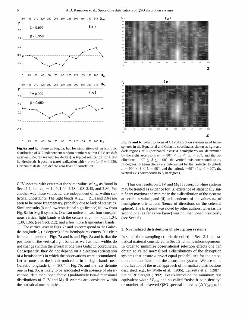
Low confidence levels for the correlation coefficients be-tween pairs of hemispheres corresponding to the longitude in-tervals105 ≤ lc ≤ 135 and285 ≤ l′c ≤ 315 are associatedwith an apparent lack of observational data in the interval of theGalactic longitudes280 <∼ l <∼ 320 (see Paper I). In the caseof Mg II systems the correlation on the2σ level occurs in onlyhalf of the 12 pairs of opposite hemispheres due to insufficientstatistics.

For comparison with the results plotted in Fig. 5a we pro-duced a few hundreds of numerical simulations of an isotropicdistribution of 312 independent random points within the in-terval of values (1.2–3.2), which corresponds to the availablestatistics of C IV absorption systems. To imitate the isotropicdistribution of absorption systems over the celestial sphere weproduce13×24 matrices for each numerical realization, where24 consecutive sets of random numbers corresponding to dif-ferent celestial sectors (∆α = 15). Boundaries between thesets (neighbor columns of the matrices) are marked by valuesαc = 0, 15, 30, .... To simulate az-distribution for the hemi-sphere with definiteαc we use13 × 12 = 156 random pointsin 12 consecutive columns around the valueαc. In this way wecalculate the correlation coefficients between the distributionsobtained in pairs of opposite hemispheres (in our simulations).

Fig. 6a shows the correlation coefficient versusαc for atypical realization. One can see that in most cases the valuesof r(αc) are noticeably lower than the valuerβ = 0.375 forβ = 0.95 (2σ confidence level).4–5 peculiar realizations were

D

β

β

αF

U

αF

E

β

β

U

"F

"F

Fig. 5a and b. Correlation coefficientr for thez-distributions of theC IV absorption systems in pairs of opposite hemispheres for Equa-torial and Galactic coordinate systems:a dependencer on the rightascensionsαc (bottom horizontal axis) andα′

c (top horizontal axis) ofthe centers of two complementary hemispheres,b dependencer on theGalactic longitudeslc (bottom horizontal axis) andl′c (top horizontalaxis) of the centers of two complementary hemispheres. The tabulatedvaluesrβ = 0.588 for the confidence levelβ = 0.999 (> 3σ) andrβ = 0.375 for β = 0.950 (2σ) are represented.

found per hundred trials with valuesr reaching the confidencelevel β = 0.95 for a restricted interval of “αc”. One such pe-culiar realization is plotted in Fig. 6b. It essentially differs fromthe valuesr(αc) plotted in Fig. 5a, wherer exceeded the con-fidence levelβ = 0.95 for all values ofαc except one. In allnumerical simulations we have failed to getr(αc) similar to thedependence represented in Fig. 5a.

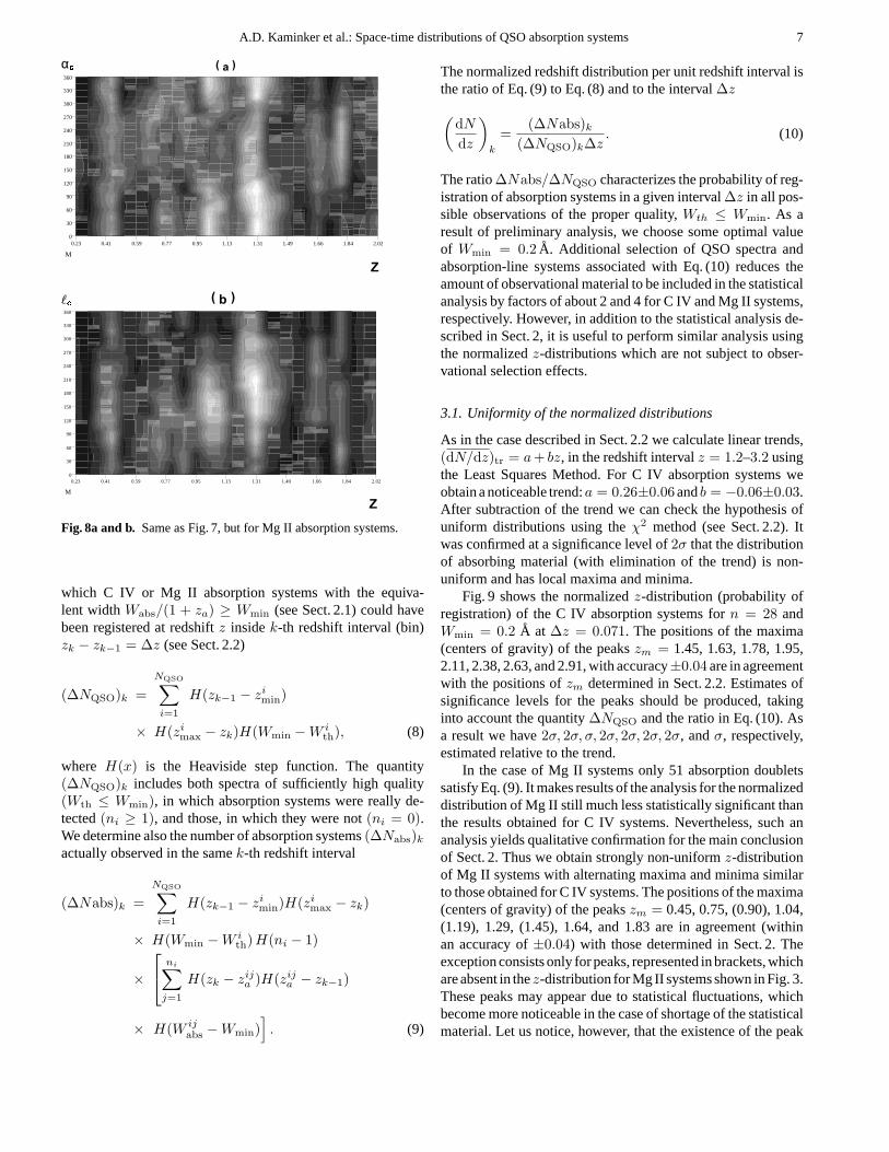
Figs. 7 and 8 show sets of the redshift distributions of theC IV and Mg II systems for the 24 hemispheres (the step ofrotations is15). They may be treated as two-dimensional dis-tributions: the vertical axes in Figs. 7a and 8a correspond to theright ascension of the hemisphere centersαc in degrees, the hor-izontal axes correspond to redshiftz. The light domains displayan enhanced number of the absorption systems per redshift bin(number density), and the dark domains display reduced numberdensities. 9 gradations of grey color were used between whitefor maximum and black for minimum of the number density.Black domains are those for which we do not have necessarydata. In Fig. 7a one can see continuous vertical light bands for

6 A.D. Kaminker et al.: Space-time distributions of QSO absorption systems

Dβ

β

αF

U

αF

Eβ

β

U

αF

αF

Fig. 6a and b. Same as Fig. 5a, but for simulations of an isotropicdistribution of 312 independent random numbers within C IV redshiftinterval 1.2–3.2 (see text for details):a typical realization for a fewhundred trials;b peculiar (rare) realization withr > rβ for β = 0.950.Horizontal dash lines denote zero level of correlation.

C IV systems with centers at the same values ofzm as found inSect. 2.2, i.e.,zm = 1.46, 1.60, 1.78, 1.98, 2.45, and2.86. Putanother way these valueszm are independent ofαc within sta-tistical uncertainty. The light bands atzm = 2.14 and2.64 areseen to be more fragmentary, probably due to lack of statistics.Similar results (but of lower statistical significance) follow fromFig. 8a for Mg II systems. One can notice at least four conspic-uous vertical light bands with the centers atzm = 0.44, 1.04,1.30, 1.66, (see Sect. 2.2), and a few more fragmentary bands.

The vertical axes in Figs. 7b and 8b correspond to the Galac-tic longitudelc (in degrees) of the hemisphere centers. It is clearfrom comparison of Figs. 7a and b, and Figs. 8a and b, that thepositions of the vertical light bands as well as their widths donot change (within the errors) if one uses Galactic coordinates.Consequently, they do not depend on a direction (orientationof a hemisphere) in which the observations were accumulated.Let us note that the break noticeable in all light bands nearGalactic longitudelc = 300 in Fig. 7b, and the less definiteone in Fig. 8b, is likely to be associated with absence of obser-vational data mentioned above. Qualitatively two-dimensionaldistributions of C IV and Mg II systems are consistent withinthe statistical uncertainties.

αk D

1.24 1.43 1.62 1.81 2.01 2.2 2.39 2.59 2.78 2.97 3.160

30

60

90

120

150

180

210

240

270

300

330

360

M

=

"k E

1.24 1.43 1.62 1.81 2.01 2.2 2.39 2.59 2.78 2.97 3.160

30

60

90

120

150

180

210

240

270

300

330

360

M

=

Fig. 7a and b. z-distributions of C IV absorption systems in 24 hemi-spheres in the Equatorial and Galactic coordinates shown as light anddark regions ofz (horizontal axis):a hemispheres are determinedby the right ascensionsαc − 90 ≤ α ≤ αc + 90, and the de-clinations−90 ≤ δ ≤ +90, the vertical axis corresponds toαc

in degrees;b hemispheres are determined by the Galactic longitudelc − 90 ≤ l ≤ lc + 90, and the latitude−90 ≤ b ≤ +90, thevertical axis corresponds tolc in degrees.

Thus our results on C IV and Mg II absorption-line systemsmay be treated as evidence for: (i) existence of statistically sig-nificant maxima and minima in thez-distribution of the systemsat certainz-values, and (ii) independence of the valueszm ofhemisphere orientations (hence of directions on the celestialsphere). The first point was noted by other authors, whereas thesecond one (as far as we know) was not mentioned previously(see Sect. 6).

3. Normalized distributions of absorption systems

In spite of the sampling criteria described in Sect. 2.1 the sta-tistical material considered in Sect. 2 remains inhomogeneous.In order to minimize observational selection effects one canobtain so called normalizedz-distributions of the absorptionsystems that ensurea priori equal probabilities for the detec-tion and identification of the absorption systems. We use somemodification of the usual approach of normalized distributionsdescribed, e.g., by Wolfe et al. (1986), Lanzetta et al. (1987),Steidel & Sargent (1992). Let us introduce the minimum restequivalent widthWmin and so called “redshift path density”or number of observed QSO spectral intervals(∆NQSO)k in

A.D. Kaminker et al.: Space-time distributions of QSO absorption systems 7

αk D

0.23 0.41 0.59 0.77 0.95 1.13 1.31 1.49 1.66 1.84 2.020

30

60

90

120

150

180

210

240

270

300

330

360

M

=

"k E

0.23 0.41 0.59 0.77 0.95 1.13 1.31 1.49 1.66 1.84 2.020

30

60

90

120

150

180

210

240

270

300

330

360

M

=

Fig. 8a and b. Same as Fig. 7, but for Mg II absorption systems.

which C IV or Mg II absorption systems with the equiva-lent widthWabs/(1 + za) ≥ Wmin (see Sect. 2.1) could havebeen registered at redshiftz insidek-th redshift interval (bin)zk − zk−1 = ∆z (see Sect. 2.2)

(∆NQSO)k =NQSO∑i=1

H(zk−1 − zimin)

× H(zimax − zk)H(Wmin − W i

th), (8)

where H(x) is the Heaviside step function. The quantity(∆NQSO)k includes both spectra of sufficiently high quality(Wth ≤ Wmin), in which absorption systems were really de-tected(ni ≥ 1), and those, in which they were not(ni = 0).We determine also the number of absorption systems(∆Nabs)k

actually observed in the samek-th redshift interval

(∆Nabs)k =NQSO∑i=1

H(zk−1 − zimin)H(zi

max − zk)

× H(Wmin − W ith) H(ni − 1)

× ni∑

j=1

H(zk − zija )H(zij

a − zk−1)

× H(W ijabs − Wmin)

]. (9)

The normalized redshift distribution per unit redshift interval isthe ratio of Eq. (9) to Eq. (8) and to the interval∆z

(dN

dz

)k

=(∆Nabs)k

(∆NQSO)k∆z. (10)

The ratio∆Nabs/∆NQSO characterizes the probability of reg-istration of absorption systems in a given interval∆z in all pos-sible observations of the proper quality,Wth ≤ Wmin. As aresult of preliminary analysis, we choose some optimal valueof Wmin = 0.2 A. Additional selection of QSO spectra andabsorption-line systems associated with Eq. (10) reduces theamount of observational material to be included in the statisticalanalysis by factors of about 2 and 4 for C IV and Mg II systems,respectively. However, in addition to the statistical analysis de-scribed in Sect. 2, it is useful to perform similar analysis usingthe normalizedz-distributions which are not subject to obser-vational selection effects.

3.1. Uniformity of the normalized distributions

As in the case described in Sect. 2.2 we calculate linear trends,(dN/dz)tr = a+ bz, in the redshift intervalz = 1.2–3.2 usingthe Least Squares Method. For C IV absorption systems weobtain a noticeable trend:a = 0.26±0.06andb = −0.06±0.03.After subtraction of the trend we can check the hypothesis ofuniform distributions using theχ2 method (see Sect. 2.2). Itwas confirmed at a significance level of2σ that the distributionof absorbing material (with elimination of the trend) is non-uniform and has local maxima and minima.

Fig. 9 shows the normalizedz-distribution (probability ofregistration) of the C IV absorption systems forn = 28 andWmin = 0.2 A at ∆z = 0.071. The positions of the maxima(centers of gravity) of the peakszm = 1.45, 1.63, 1.78, 1.95,2.11, 2.38, 2.63, and 2.91, with accuracy±0.04 are in agreementwith the positions ofzm determined in Sect. 2.2. Estimates ofsignificance levels for the peaks should be produced, takinginto account the quantity∆NQSO and the ratio in Eq. (10). Asa result we have2σ, 2σ, σ, 2σ, 2σ, 2σ, 2σ, andσ, respectively,estimated relative to the trend.

In the case of Mg II systems only 51 absorption doubletssatisfy Eq. (9). It makes results of the analysis for the normalizeddistribution of Mg II still much less statistically significant thanthe results obtained for C IV systems. Nevertheless, such ananalysis yields qualitative confirmation for the main conclusionof Sect. 2. Thus we obtain strongly non-uniformz-distributionof Mg II systems with alternating maxima and minima similarto those obtained for C IV systems. The positions of the maxima(centers of gravity) of the peakszm = 0.45, 0.75, (0.90), 1.04,(1.19), 1.29, (1.45), 1.64, and 1.83 are in agreement (withinan accuracy of±0.04) with those determined in Sect. 2. Theexception consists only for peaks, represented in brackets, whichare absent in thez-distribution for Mg II systems shown in Fig. 3.These peaks may appear due to statistical fluctuations, whichbecome more noticeable in the case of shortage of the statisticalmaterial. Let us notice, however, that the existence of the peak

8 A.D. Kaminker et al.: Space-time distributions of QSO absorption systems

∆1 DEV ∆1 4

62

=

&,9

D

∆1 DEV

∆1462

=

E

Fig. 9a and b. Same as Fig. 2, but for the normalized distribution∆Nabs/∆NQSO.

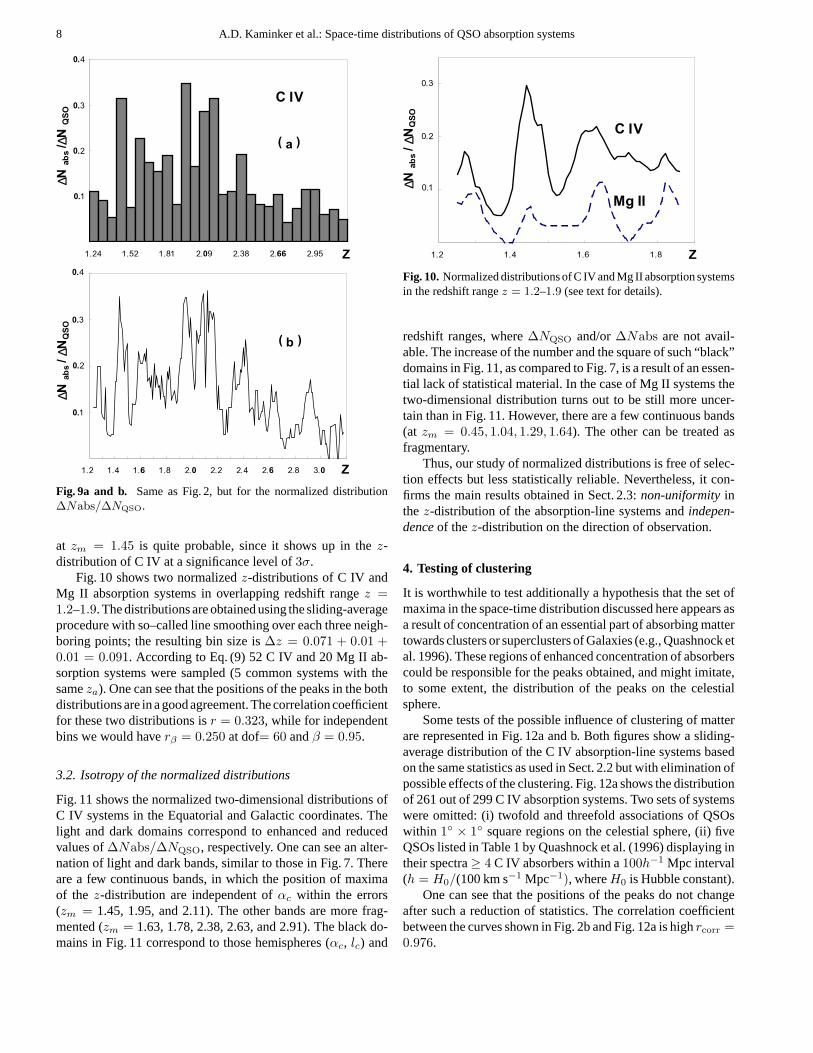
at zm = 1.45 is quite probable, since it shows up in thez-distribution of C IV at a significance level of3σ.

Fig. 10 shows two normalizedz-distributions of C IV andMg II absorption systems in overlapping redshift rangez =1.2–1.9. The distributions are obtained using the sliding-averageprocedure with so–called line smoothing over each three neigh-boring points; the resulting bin size is∆z = 0.071 + 0.01 +0.01 = 0.091. According to Eq. (9) 52 C IV and 20 Mg II ab-sorption systems were sampled (5 common systems with thesameza). One can see that the positions of the peaks in the bothdistributions are in a good agreement. The correlation coefficientfor these two distributions isr = 0.323, while for independentbins we would haverβ = 0.250 at dof= 60 andβ = 0.95.

3.2. Isotropy of the normalized distributions

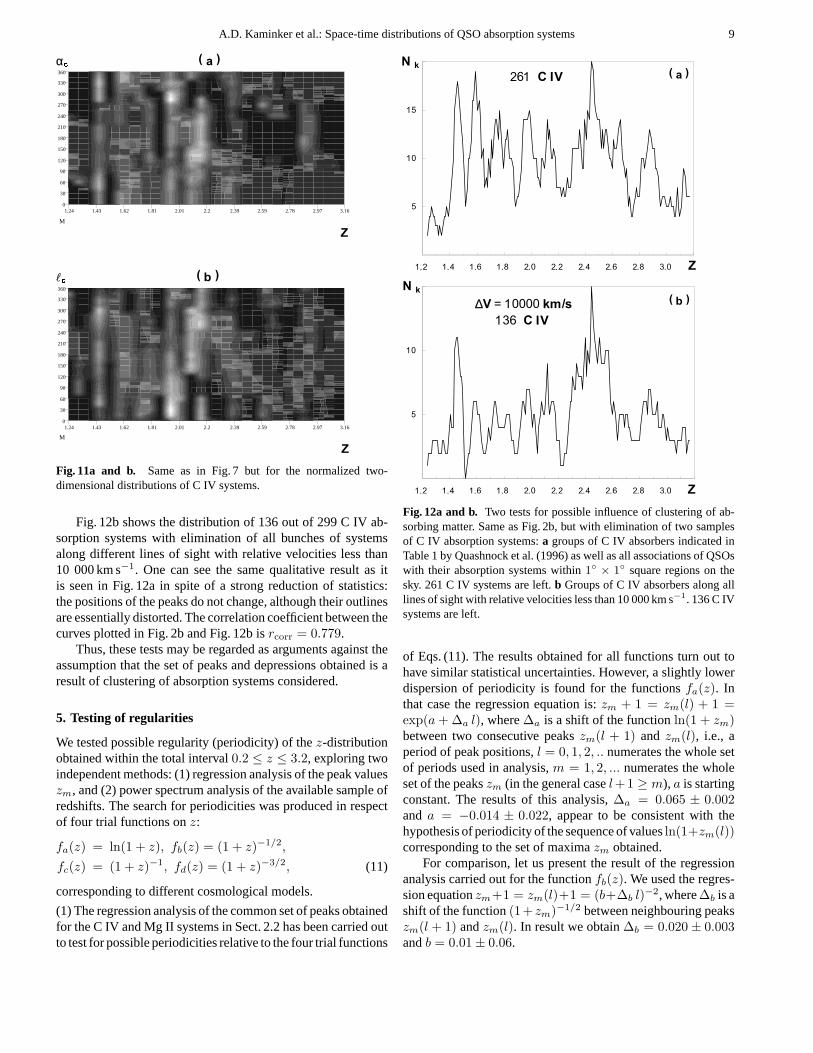
Fig. 11 shows the normalized two-dimensional distributions ofC IV systems in the Equatorial and Galactic coordinates. Thelight and dark domains correspond to enhanced and reducedvalues of∆Nabs/∆NQSO, respectively. One can see an alter-nation of light and dark bands, similar to those in Fig. 7. Thereare a few continuous bands, in which the position of maximaof the z-distribution are independent ofαc within the errors(zm = 1.45, 1.95, and 2.11). The other bands are more frag-mented (zm = 1.63, 1.78, 2.38, 2.63, and 2.91). The black do-mains in Fig. 11 correspond to those hemispheres (αc, lc) and

∆1 DEV

∆1462

=

&,9

0J,,

Fig. 10. Normalized distributions of C IV and Mg II absorption systemsin the redshift rangez = 1.2–1.9 (see text for details).

redshift ranges, where∆NQSO and/or∆Nabs are not avail-able. The increase of the number and the square of such “black”domains in Fig. 11, as compared to Fig. 7, is a result of an essen-tial lack of statistical material. In the case of Mg II systems thetwo-dimensional distribution turns out to be still more uncer-tain than in Fig. 11. However, there are a few continuous bands(at zm = 0.45, 1.04, 1.29, 1.64). The other can be treated asfragmentary.

Thus, our study of normalized distributions is free of selec-tion effects but less statistically reliable. Nevertheless, it con-firms the main results obtained in Sect. 2.3:non-uniformityinthe z-distribution of the absorption-line systems andindepen-denceof thez-distribution on the direction of observation.

4. Testing of clustering

It is worthwhile to test additionally a hypothesis that the set ofmaxima in the space-time distribution discussed here appears asa result of concentration of an essential part of absorbing mattertowards clusters or superclusters of Galaxies (e.g., Quashnock etal. 1996). These regions of enhanced concentration of absorberscould be responsible for the peaks obtained, and might imitate,to some extent, the distribution of the peaks on the celestialsphere.

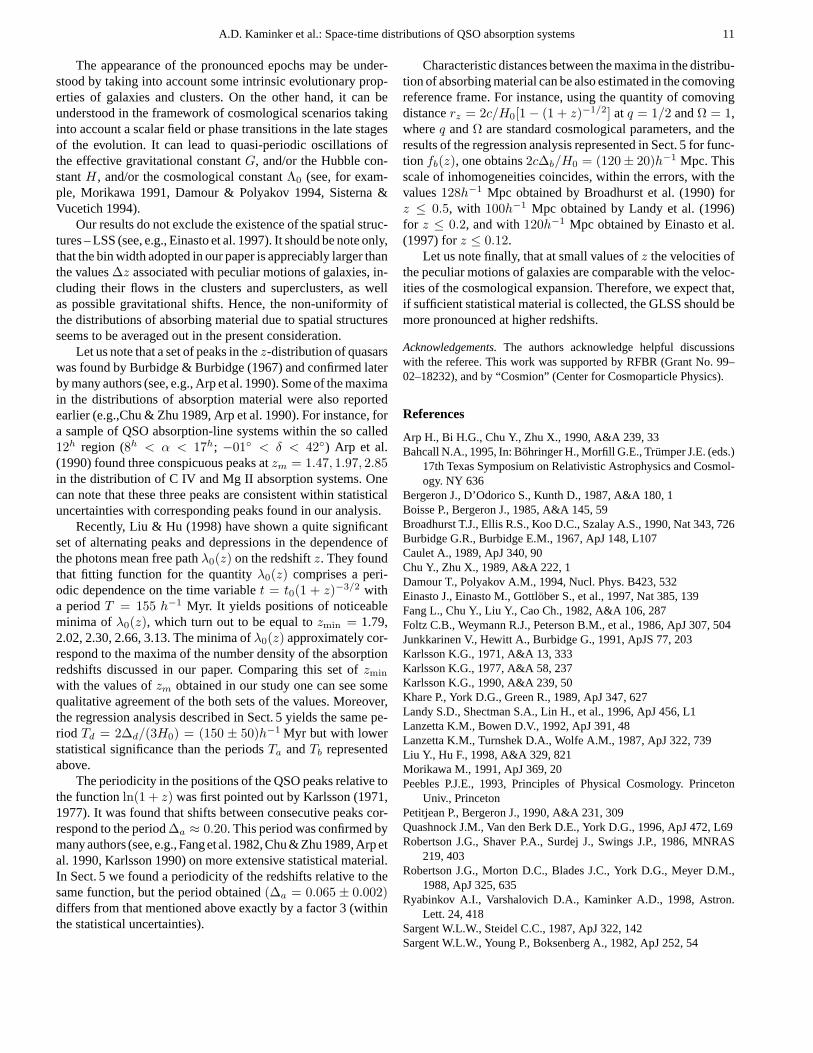
Some tests of the possible influence of clustering of matterare represented in Fig. 12a and b. Both figures show a sliding-average distribution of the C IV absorption-line systems basedon the same statistics as used in Sect. 2.2 but with elimination ofpossible effects of the clustering. Fig. 12a shows the distributionof 261 out of 299 C IV absorption systems. Two sets of systemswere omitted: (i) twofold and threefold associations of QSOswithin 1 × 1 square regions on the celestial sphere, (ii) fiveQSOs listed in Table 1 by Quashnock et al. (1996) displaying intheir spectra≥ 4 C IV absorbers within a100h−1 Mpc interval(h = H0/(100 km s−1 Mpc−1), whereH0 is Hubble constant).

One can see that the positions of the peaks do not changeafter such a reduction of statistics. The correlation coefficientbetween the curves shown in Fig. 2b and Fig. 12a is highrcorr =0.976.

A.D. Kaminker et al.: Space-time distributions of QSO absorption systems 9

αk D

1.24 1.43 1.62 1.81 2.01 2.2 2.39 2.59 2.78 2.97 3.160

30

60

90

120

150

180

210

240

270

300

330

360

M

=

"k E

1.24 1.43 1.62 1.81 2.01 2.2 2.39 2.59 2.78 2.97 3.160

30

60

90

120

150

180

210

240

270

300

330

360

M

=

Fig. 11a and b. Same as in Fig. 7 but for the normalized two-dimensional distributions of C IV systems.

Fig. 12b shows the distribution of 136 out of 299 C IV ab-sorption systems with elimination of all bunches of systemsalong different lines of sight with relative velocities less than10 000 km s−1. One can see the same qualitative result as itis seen in Fig. 12a in spite of a strong reduction of statistics:the positions of the peaks do not change, although their outlinesare essentially distorted. The correlation coefficient between thecurves plotted in Fig. 2b and Fig. 12b isrcorr = 0.779.

Thus, these tests may be regarded as arguments against theassumption that the set of peaks and depressions obtained is aresult of clustering of absorption systems considered.

5. Testing of regularities

We tested possible regularity (periodicity) of thez-distributionobtained within the total interval0.2 ≤ z ≤ 3.2, exploring twoindependent methods: (1) regression analysis of the peak valueszm, and (2) power spectrum analysis of the available sample ofredshifts. The search for periodicities was produced in respectof four trial functions onz:

fa(z) = ln(1 + z), fb(z) = (1 + z)−1/2,

fc(z) = (1 + z)−1, fd(z) = (1 + z)−3/2, (11)

corresponding to different cosmological models.

(1) The regression analysis of the common set of peaks obtainedfor the C IV and Mg II systems in Sect. 2.2 has been carried outto test for possible periodicities relative to the four trial functions

1N

=

D&,9

1N

=

∆9 NPV

&,9

E

Fig. 12a and b. Two tests for possible influence of clustering of ab-sorbing matter. Same as Fig. 2b, but with elimination of two samplesof C IV absorption systems:a groups of C IV absorbers indicated inTable 1 by Quashnock et al. (1996) as well as all associations of QSOswith their absorption systems within1 × 1 square regions on thesky. 261 C IV systems are left.b Groups of C IV absorbers along alllines of sight with relative velocities less than 10 000 km s−1. 136 C IVsystems are left.

of Eqs. (11). The results obtained for all functions turn out tohave similar statistical uncertainties. However, a slightly lowerdispersion of periodicity is found for the functionsfa(z). Inthat case the regression equation is:zm + 1 = zm(l) + 1 =exp(a + ∆a l), where∆a is a shift of the functionln(1 + zm)between two consecutive peakszm(l + 1) and zm(l), i.e., aperiod of peak positions,l = 0, 1, 2, .. numerates the whole setof periods used in analysis,m = 1, 2, ... numerates the wholeset of the peakszm (in the general casel+1 ≥ m), a is startingconstant. The results of this analysis,∆a = 0.065 ± 0.002and a = −0.014 ± 0.022, appear to be consistent with thehypothesis of periodicity of the sequence of valuesln(1+zm(l))corresponding to the set of maximazm obtained.

For comparison, let us present the result of the regressionanalysis carried out for the functionfb(z). We used the regres-sion equationzm+1 = zm(l)+1 = (b+∆b l)−2, where∆b is ashift of the function(1+ zm)−1/2 between neighbouring peakszm(l + 1) andzm(l). In result we obtain∆b = 0.020 ± 0.003andb = 0.01 ± 0.06.

10 A.D. Kaminker et al.: Space-time distributions of QSO absorption systems

OQ]

3P

P

]−

3P

P

]−

3P

P

]−

3P

P

Fig. 13. Power spectraP (m), m is number of harmonics, for thecommonz-distribution of C IV and Mg II systems (z = 0.2–3.2)obtained for four trial functions (see Eqs. (11)) indicated in each panel.Horizontal dashed lines denote confidence levelβ = 0.950.

(2) The power spectrum analysis was used to test periodicitieswith respect to the trial functions of Eqs. (11) for the sample ofC IV and Mg II redshifts. This technique is independent of theprocedures used in our previous analysis. The spectral power isdefined in a standard way (see, e.g., Karlsson 1977, Arp et al.1990):

P(m) =1N

[N∑

i=1

cos(

2πmf(zi)F

)]2

+

[N∑

i=1

sin(

2πmf(zi)F

)]2 , (12)

whereN = 497 is the number of redshift values usedzi (i =1, 2..N), f(zi) = fa(zi), ...fd(zi) are the trial functions givenin Eq. (11),F = f(zN )−f(z1) is the total interval of variationsof f(zi), m is harmonic number. The existence of periodicityappears as a peak in the power spectrumP = max (P(m)) witha confidence probability

β ≥ [1 − exp(−P)]N/2, (13)

whereN/2 is the maximum number of possible peaks (period-icities) in az-distribution ofN redshifts.

The results of this analysis for all trial functions given byEqs. (11) are represented in Fig. 13. One can see that in theinterval ofm considered the only significant peakP(m) appearsfor the functionf(z) = fa(z) atm = 19 on the confidence levelβ = 0.973 (> 2σ). This peak corresponds to a periodicity ofthe distribution in respect to the functionln(1+z) with a period∆a = F/m = 0.066 ± 0.003. This is quite consistent with theresult of the regression analysis given above.

Let us note that the power spectrum analysis does not dependon the choice of redshift bin and may be treated as additionalevidence for the existence of the peak-depression structure forthe redshifts distribution discussed in Sect. 2.2.

6. Discussion and conclusions

The statistical analysis of the distributions of C IV and Mg IIabsorption-line systems with redshiftsz = 0.2–3.2 leads to thefollowing conclusions.

(1) The distributions of the absorption systems are not uniform(at the confidence levelβ > 0.998), and have alternating max-ima and minima. The maxima in the distribution of C IV systemscorrespond tozm = 1.46, 1.60, 1.78, 1.98, 2.14, 2.45, 2.64, and2.86(±0.04). The maxima in the distribution of Mg II systemsappear atzm = 0.44, 0.77, 1.04, 1.30, 1.66, and 1.78(±0.04).Most of these peaks have a significance> 2σ, however, someof them are less significant, probably due to lack of statistics.

(2) Values of zm corresponding to the maxima of thez-distributions were found to be independent (within statisticaluncertainties) of hemisphere orientations. In particular, there isa correlation of thez-distributions in pairs of opposite (inde-pendent) hemispheres on a significance level>∼ 2σ. This isevidence of statistical isotropy of the distributions.

(3) The distribution obtained can be imagined as a series ofembedded spheres of absorbing material (onion-like structure)corresponding to the peaks atzm indicated above. Such structuremay be considered as a Global Large-Scale Structure (GLSS) ofthe space-time distribution, and most likely is associated with anappearance of pronounced and depressed epochs in the courseof cosmological evolution.

(4) The characteristic time intervalT between the maximaof pronounced epochs strongly depends on the cosmologicalmodel and on a trial function used (see Sect. 5). For instance,one can estimate thatTa = ∆a/H0 = (650 ± 30)h−1 Myr forthe trial functionfa(z) from Eq. (11), andTb = 2∆b/H0 =(400 ± 60)h−1 Myr for the trial functionfb(z).

Let us stress that there is no contradiction between the GLLSconsidered and the statement that all points of space are equiva-lent. The GLLS does not correspond to a fixed cosmic time, butdisplays the time evolution. As an example of the pronouncedepochs appearing as isotropic elements of the GLSS one mayconsidered the epoch of the hydrogen recombination associatedwith formation of the Cosmic Microwave Background.

A.D. Kaminker et al.: Space-time distributions of QSO absorption systems 11

The appearance of the pronounced epochs may be under-stood by taking into account some intrinsic evolutionary prop-erties of galaxies and clusters. On the other hand, it can beunderstood in the framework of cosmological scenarios takinginto account a scalar field or phase transitions in the late stagesof the evolution. It can lead to quasi-periodic oscillations ofthe effective gravitational constantG, and/or the Hubble con-stantH, and/or the cosmological constantΛ0 (see, for exam-ple, Morikawa 1991, Damour & Polyakov 1994, Sisterna &Vucetich 1994).

Our results do not exclude the existence of the spatial struc-tures – LSS (see, e.g., Einasto et al. 1997). It should be note only,that the bin width adopted in our paper is appreciably larger thanthe values∆z associated with peculiar motions of galaxies, in-cluding their flows in the clusters and superclusters, as wellas possible gravitational shifts. Hence, the non-uniformity ofthe distributions of absorbing material due to spatial structuresseems to be averaged out in the present consideration.

Let us note that a set of peaks in thez-distribution of quasarswas found by Burbidge & Burbidge (1967) and confirmed laterby many authors (see, e.g., Arp et al. 1990). Some of the maximain the distributions of absorption material were also reportedearlier (e.g.,Chu & Zhu 1989, Arp et al. 1990). For instance, fora sample of QSO absorption-line systems within the so called12h region (8h < α < 17h; −01 < δ < 42) Arp et al.(1990) found three conspicuous peaks atzm = 1.47, 1.97, 2.85in the distribution of C IV and Mg II absorption systems. Onecan note that these three peaks are consistent within statisticaluncertainties with corresponding peaks found in our analysis.

Recently, Liu & Hu (1998) have shown a quite significantset of alternating peaks and depressions in the dependence ofthe photons mean free pathλ0(z) on the redshiftz. They foundthat fitting function for the quantityλ0(z) comprises a peri-odic dependence on the time variablet = t0(1 + z)−3/2 witha periodT = 155 h−1 Myr. It yields positions of noticeableminima of λ0(z), which turn out to be equal tozmin = 1.79,2.02, 2.30, 2.66, 3.13. The minima ofλ0(z) approximately cor-respond to the maxima of the number density of the absorptionredshifts discussed in our paper. Comparing this set ofzminwith the values ofzm obtained in our study one can see somequalitative agreement of the both sets of the values. Moreover,the regression analysis described in Sect. 5 yields the same pe-riod Td = 2∆d/(3H0) = (150 ± 50)h−1 Myr but with lowerstatistical significance than the periodsTa andTb representedabove.

The periodicity in the positions of the QSO peaks relative tothe functionln(1 + z) was first pointed out by Karlsson (1971,1977). It was found that shifts between consecutive peaks cor-respond to the period∆a ≈ 0.20. This period was confirmed bymany authors (see, e.g., Fang et al. 1982, Chu & Zhu 1989, Arp etal. 1990, Karlsson 1990) on more extensive statistical material.In Sect. 5 we found a periodicity of the redshifts relative to thesame function, but the period obtained(∆a = 0.065 ± 0.002)differs from that mentioned above exactly by a factor 3 (withinthe statistical uncertainties).

Characteristic distances between the maxima in the distribu-tion of absorbing material can be also estimated in the comovingreference frame. For instance, using the quantity of comovingdistancerz = 2c/H0[1 − (1 + z)−1/2] at q = 1/2 andΩ = 1,whereq andΩ are standard cosmological parameters, and theresults of the regression analysis represented in Sect. 5 for func-tion fb(z), one obtains2c∆b/H0 = (120 ± 20)h−1 Mpc. Thisscale of inhomogeneities coincides, within the errors, with thevalues128h−1 Mpc obtained by Broadhurst et al. (1990) forz ≤ 0.5, with 100h−1 Mpc obtained by Landy et al. (1996)for z ≤ 0.2, and with120h−1 Mpc obtained by Einasto et al.(1997) forz ≤ 0.12.

Let us note finally, that at small values ofz the velocities ofthe peculiar motions of galaxies are comparable with the veloc-ities of the cosmological expansion. Therefore, we expect that,if sufficient statistical material is collected, the GLSS should bemore pronounced at higher redshifts.

Acknowledgements.The authors acknowledge helpful discussionswith the referee. This work was supported by RFBR (Grant No. 99–02–18232), and by “Cosmion” (Center for Cosmoparticle Physics).

References

Arp H., Bi H.G., Chu Y., Zhu X., 1990, A&A 239, 33Bahcall N.A., 1995, In: Bohringer H., Morfill G.E., Trumper J.E. (eds.)

17th Texas Symposium on Relativistic Astrophysics and Cosmol-ogy. NY 636

Bergeron J., D’Odorico S., Kunth D., 1987, A&A 180, 1Boisse P., Bergeron J., 1985, A&A 145, 59Broadhurst T.J., Ellis R.S., Koo D.C., Szalay A.S., 1990, Nat 343, 726Burbidge G.R., Burbidge E.M., 1967, ApJ 148, L107Caulet A., 1989, ApJ 340, 90Chu Y., Zhu X., 1989, A&A 222, 1Damour T., Polyakov A.M., 1994, Nucl. Phys. B423, 532Einasto J., Einasto M., Gottlober S., et al., 1997, Nat 385, 139Fang L., Chu Y., Liu Y., Cao Ch., 1982, A&A 106, 287Foltz C.B., Weymann R.J., Peterson B.M., et al., 1986, ApJ 307, 504Junkkarinen V., Hewitt A., Burbidge G., 1991, ApJS 77, 203Karlsson K.G., 1971, A&A 13, 333Karlsson K.G., 1977, A&A 58, 237Karlsson K.G., 1990, A&A 239, 50Khare P., York D.G., Green R., 1989, ApJ 347, 627Landy S.D., Shectman S.A., Lin H., et al., 1996, ApJ 456, L1Lanzetta K.M., Bowen D.V., 1992, ApJ 391, 48Lanzetta K.M., Turnshek D.A., Wolfe A.M., 1987, ApJ 322, 739Liu Y., Hu F., 1998, A&A 329, 821Morikawa M., 1991, ApJ 369, 20Peebles P.J.E., 1993, Principles of Physical Cosmology. Princeton

Univ., PrincetonPetitjean P., Bergeron J., 1990, A&A 231, 309Quashnock J.M., Van den Berk D.E., York D.G., 1996, ApJ 472, L69Robertson J.G., Shaver P.A., Surdej J., Swings J.P., 1986, MNRAS

219, 403Robertson J.G., Morton D.C., Blades J.C., York D.G., Meyer D.M.,

1988, ApJ 325, 635Ryabinkov A.I., Varshalovich D.A., Kaminker A.D., 1998, Astron.

Lett. 24, 418Sargent W.L.W., Steidel C.C., 1987, ApJ 322, 142Sargent W.L.W., Young P., Boksenberg A., 1982, ApJ 252, 54

12 A.D. Kaminker et al.: Space-time distributions of QSO absorption systems

Sargent W.L.W., Boksenberg A., Steidel C.C., 1988a, ApJS 68, 539Sargent W.L.W., Steidel C.C., Boksenberg A., 1988b, ApJ 334, 22Sargent W.L.W., Steidel C.C., Boksenberg A., 1989, ApJS 69, 703Sargent W.L.W., Steidel C.C., Boksenberg A., 1990, ApJ 351, 364Sisterna P.D., Vucetich H., 1994, Phys. Rev. Lett. 72, 454Steidel C.C., 1990, ApJS 72, 1

Steidel C.C., Sargent W.L.W., 1992, ApJS 80, 1Turnshek, D.A., Wolfe A.M., Lanzetta K.M., et al., 1989, ApJ 344, 567Val’tts I.E., 1991, AZh 68, 261Wolfe A.M., Turnshek D.A., Smith H.E., Cohen R.D., 1986, ApJS 61,

249Young P., Sargent W.L.W., Boksenberg A., 1982, ApJ 252, 10