astr

o-ph

/960

2100

v2

17

Dec

199

6

Mon. Not. R. Astron. Soc. 000, 000{000 (1996)

Reconstruction of cosmological density and velocity �elds

in the Lagrangian Zel'dovich Approximation

Rupert A.C. Croft

1

and Enrique Gazta~naga

2;3

1

Department of Astronomy, The Ohio State University, Columbus, Ohio 43210, USA

2

Research Unit (CSIC), Institut d'Estudis Espacials de Catalunyaq (IEEC), Edf. Nexus-104 - c/ Gran Capitan 2-4, 08034 Barcelona

3

Oxford University, Astrophysics, Keble Road, Oxford OX1 3RH, UK

16 December 1996

ABSTRACT

We present a method for reconstructing cosmological density and velocity �elds using

the Lagrangian Zel'dovich formalism. The method involves �nding the least action

solution for straight line particle paths in an evolving density �eld. Our starting point is

the �nal, evolved density , so that we are in e�ect carrying out the standard Zel'dovich

Approximation based process in reverse. Using a simple numerical algorithm we are

able to minimise the action for the trajectories of several million particles. We apply

our method to the evolved density taken from N-body simulations of di�erent cold dark

matter dominated universes, testing both the prediction for the present day velocity �eld

and for the initial density �eld. The method is easy to apply, reproduces the accuracy

of the forward Zel'dovich Approximation, and also works directly in redshift space with

minimal modi�cation.

Key words: Large-scale structure of the universe { galaxies: clustering, methods:

numerical, statistical.

1 INTRODUCTION

Structure in the present day Universe is believed to have

been formed as a result of the growth of small amplitude

energy-density perturbations in the early Universe via the

mechanism of gravitational instability. On scales signi�-

cantly larger than individual galaxies we expect gravity to be

the dominant e�ect so that we can use gravitational dynam-

ics to relate theoretical predictions for the initial uctuations

with the present day observed Universe. These observations

are mainly of the spatial distribution of galaxies, from red-

shift surveys (e.g. Davis & Peebles 1983, Fisher et al. 1994).

With the above assumption, we can in principle use our

knowledge of gravity to recover the initial conditions and

compare with theories for the generation of initial uctua-

tions, such as in ation which predicts a Gaussian distribu-

tion of Fourier amplitudes. In this paper, we present a simple

method for doing this, which uses as its starting point the

present day positions of galaxies in redshift space.

Prior to a redshift of z� 10

3

, the nature of dark matter

will have been important in the evolution of uctuations

and this will also be re ected in the initial conditions Direct

measurements of galaxy peculiar velocities (Dressler et al.

1987, Burstein 1990, Willick et al. 1995) and comparisons

with predictions of gravitational instability can provide an

important consistency check on the above procedure.

Methods for determining the gravitational evolution of

cosmological density perturbations can be split into two cat-

egories - the Eulerian and Lagrangian approaches. In the

Eulerian approach (see e.g. Lifshitz 1946, Peebles 1980) so-

lutions to the equations for the force, conservation of mat-

ter, and Poisson's equation are sought in comoving coor-

dinates as a function of the dimensionless density contrast

�(x; t) = [�(x; t) � �]=�. This variable can be expanded as

a perturbation series (eg Peebles 1980), with solutions that

are valid as long as j�(x; t)j � 1. When taken to the �rst

order, i.e. linear theory, uctuations grow at the same rate

everywhere: �(x; t) / D(t).

In the Lagrangian formalism, the variable under con-

sideration is the displacement of a particle or uid element

from its initial position. This approach was pioneered by

Zel'dovich (1970) who suggested that the relation between

a particle's initial Lagrangian coordinate q and the �nal Eu-

lerian coordinate x could be approximated by

x(q; t) = q +D(t)(q): (1)

Here the vector (q) is a time-independent function of the

Lagrangian density �eld and D(t) is the growth factor for

linear modes (see Section 2). An advantage compared to

Eulerian theory is that the displacement remains �nite at all

times, even when �(x; t) ! 1 at orbit crossing. Although

2 R.A.C. Croft and E. Gazta~naga

displacements everywhere grow at the same rate, governed

by D(t), the rate of growth of density perturbations varies

as a function of position. This enables this approximation

to capture some dynamical e�ects of the weakly non-linear

regime.

In higher order Lagrangian theories (see eg Moutarde

etal 1991, Bouchet et al. 1995, Catelan 1995) it is possible to

treat the total displacement �eld as an expansion. There are

however some problems with using such asymptotic series.

For example Sahni and Shandarin (1995) show that the �rst

order Lagrangian pertubation theory performs better than

higher order Lagrangian theories in predicting the evolution

of voids at late times. In this paper we will limit ourselves

to the �rst order (the Zel'dovich Approximation). This has

been shown to be surprisingly accurate, given its simplicity

(see tests on N -body simulations by e.g. Doroshkevich et al.

(1980), Efstathiou et al. (1985), Coles, Melott & Shandarin

(1993)). It also has the important advantage that particles

move in straight lines which enables us to use a simple com-

putational method (see Section 2).

So far we have mentioned approximate methods which

are mainly used to evolve an initial mass distribution sub-

ject to gravity forward in time. If we restrict ourselves to

the growing mode of uctuations we can in principle use

them to recover the initial density. In Eulerian linear the-

ory, the situation is trivial as the initial density is simply a

scaled version of the �nal density. The Zel'dovich Approx-

imation (hereafter ZA) has been recast in Eulerian coordi-

nates and used as a tool for reconstructing the initial condi-

tions by Nusser and Dekel (1992) and Gramman (1993a,b).

The method of Nusser and Dekel is based on the require-

ment of momentum conservation in the ZA which is used to

derive the Bernoulli equation for the evolution of the veloc-

ity potential. The approach of Gramman (1993a,b) is di�er-

ent, and in some respects closer to the particle trajectory

based ZA as mass conservation is required. The resulting

Zel'dovich-Continuity equation yields results that are more

accurate than those of Nusser and Dekel, although at the

expense of increased complexity.

Peebles (1989) pioneered the use of Hamilton's princi-

ple, that the action is minimised during the evolution of a

collection of particles or a density �eld under gravity. This

principle was used together with the assumption that the

initial peculiar velocities of galaxies are zero in order to pre-

dict galaxy orbits in the local group (Peebles 1989) and for

galaxies within 3000 kms

�1

(Shaya, Peebles and Tully 1995).

Giavalisco (1993) and Susperregi and Binney (1994) also use

least action in the context of an evolving mass distribution,

in the latter case applied to mass smoothed onto an Eulerian

grid.

Other methods of reconstructing initial conditions in-

clude that of Weinberg (1992) which involves a monotonic

mapping of the �nal smoothed density back to the initial

density on the assumption that rank order of density con-

trasts is preserved.

In this paper, we will use the principle of least action to

describe the evolution of particle trajectories. We shall do

this in the framework of the Lagrangian (particle based) ZA,

which as we shall see is the least action solution for straight

line particle paths. Our reasons for using this approach are

as follows.

� After Eulerian linear theory, the Lagrangian ZA is proba-

bly the most used and most studied dynamical scheme, and

yet it hasn't been applied to evolved density �elds.

� The forward implementation of the ZA is easy to apply

and computationally simple, features that we can hope to

retain with an inverse ZA.

� Procedures that work in Eulerian space usually require

the density �eld to be smoothed prior to carrying out the

reconstruction. The smoothing procedure does not in gen-

eral commute with the non-linear operations that are carried

out on the density �eld. With a Lagrangian approach we can

carry out the smoothing after the reconstruction.

� In principle it should be simple to make a Lagrangian

procedure work in redshift space. We just need to add the

predicted line-of-sight velocity for each particle to its posi-

tion.

The layout of this paper is as follows. In Section 2 we

examine the relationship between the principle of least ac-

tion and the ZA. We describe our scheme for recovering the

displacements from a �nal density �eld. In Section 3 we test

the scheme on N-body simulations of CDM universes. We

examine the recovery of the displacements and the predic-

tion for the �nal velocity �eld. We then test the recovery

of the initial density �eld. In the last two parts of this sec-

tion we brie y examine how successful the scheme is when

applied to a density �eld in redshift space and also when

applied to a biased density �eld. In Section 4 we discuss our

results further, and outline some suggestions for improve-

ments and further work. Our conclusions are summarised in

Section 5.

2 LEAST ACTION AND THE ZEL'DOVICH

APPROXIMATION

We �rst consider a nonrelativistic set of particles with

masses m

i

and comoving coordinates x

i

in an expanding

universe where non-gravitational forces can be ignored. The

equations of motion can be obtained from the stationary

points that result when varying the action with respect to

particle trajectories. The action S is given by the integral of

the particles' Lagrangian L over time, so that

S =

Z

t

0

dt L =

Z

t

0

dt [K �W]: (2)

The kinetic energy K is given by:

K =

1

2

X

m

i

a

2

_x

2

i

(3)

with a = a(t) � (1 + z)

�1

the universal expansion fac-

tor, which for a non-relativistic matter dominated universe

obeys:

_a

a

� H = H

0

�

0

=a

3

+ (1�

0

�

�

)=a

2

+

�

�

1=2

0

=

8�G�

0

3H

2

0

;

�

=

�

3H

2

0

: (4)

HereH

0

and �

0

are the present values of the Hubble constant

and background density, and � is the cosmological constant.

The gravitational potential energy W in an expanding

universe can be written as an integral function of the mass

autocorrelation function:

Cosmological density and velocity �elds 3

W = �

1

2

G a

�1

1

V

Z

dV �

2

(r)=r: (5)

The energy conservation equation for the Lagrangian can be

rewritten as:

d

dt

a(K +W) = �K _a (6)

(see e.g. Peebles 1980).

2.1 Straight line particle paths

We next introduce the following ansatz for the dynamics of

each particle:

x

i

(t) = x

i

(0) + F (t)

i

(7)

where F (t) is an universal function of time and

i

is some

small initial displacement. If we assume that the initial ve-

locities can be neglected,_x

i

(0) ' 0, the comoving velocity

of each particle is given by:

_x

i

=

_

F (t)

i

=

_

F

F

�x

i

; (8)

Particles therefore move with rectilinear trajectories (al-

though their velocities are a function of time). In the linear

regime, mass conservation requires that �(x

i

) / F , which

means that F (t) = D(t) is the linear growth factor:

D(t) =

_a

a

Z

a

0

da _a

�3

(9)

(see e.g. Peebles 1980), which can be readily integrated using

equation (4). In this case we recover the ZA of equation (1)

in the form:

_x

i

= f H �x

i

; (10)

where f � (a

_

D)=( _aD) is the standard linear growth factor

for velocities. A reasonable approximation to f is f '

0:6

(Peebles 1980), although this can become slightly inaccurate

if the Universe has a non zero cosmological constant (Lahav

et al. 1991) .

This ansatz can be used to estimate the displacement

�eld and corresponding velocity �eld from a given particle

distribution, as follows. The kinetic energy can be written

as:

K =

1

2

a

2

_

F

2

X

m

i

2

i

�

1

2

a

2

_

F

2

2

0

; (11)

which de�nes the mean square particle displacement

2

0

.

>From the energy conservation equation (6) we �nd:

W = �K �

2

0

2 a

Z

a

0

da a

2

_

F

2

; (12)

so that the action is given by:

S =

2

0

Z

1

0

da

_a

�

a

2

_

F

2

+

1

2 a

Z

a

0

da a

2

_

F

2

�

: (13)

In this situation K, W, the Lagrangian L and the action

S are proportional to

2

0

multiplied by a universal func-

tion of time that is �xed by the cosmology. Thus the least

action principle requires the minimum mean square particle

displacement

2

0

between the initial and �nal conditions. In

this paper we will use this result to estimate the set of

i

(or �x

i

) that minimize

2

0

for a given �nal particle dis-

tribution x

i

on assumption that the initial distribution is

homogenous.

2.2 The Zel'dovich Approximation

The least action argument above holds for an arbitrary func-

tion F (t) in equation (7), although the resulting solution is

not necessarily a good approximation to the exact equations

of motion. The choice F (t) = D(t) produces a consistent

reconstruction in the quasi-linear regime, i.e. the Zel'dovich

Approximation. In general there could be further non-linear

corrections, and F (t) might di�er from D(t). Note never-

theless that one would expect corrections to be smaller for

_

D=D than for D, which is why the approximation should be

better than plain linear theory.

One could generalize the ZA by considering a more gen-

eral expression with higher order polynomials in the linear

growth function:

F (t) ' D(t) + �D(t)

2

+ ::: (14)

which reproduces the ZA in the limit D(t) ! 0.

?

The �rst

order correction to the velocities is then:

_x

i

= f H (1 + �D) �x

i

: (15)

The value of � can be estimated by a further minimiza-

tion of the action (13) with respect to F , which yields:

d

dt

�

a

2

_

F

�

F +

1

2a

Z

a

0

da a

2

_

F

�

F

�

= 0: (16)

We �nd that for F = D+�D

2

, with D given by equation (9),

the solution of the above equation is � = 0. Thus, the

Zel'dovich Approximation F (t) = D(t) provides the min-

imal action for straight line particle paths, which justi�es,

beyond the linear regime, the use of equation (10) to predict

the velocities in terms of the displacements.

We have chosen to approach the problem of reconstruc-

tion of the true displacements from a purely dynamical per-

spective. It is also possible to appeal to more general con-

siderations to recover the true displacements for situations

in which there is no shell crossing. In Appendix A1 we show

how the abscence of shell crossing in a con�guration of par-

ticle trajectories determines that that con�guration has the

minimum mean squared displacement of all possible con�g-

urations. One consequence of this is that we could also re-

cover the particle displacements caused by non-gravitational

mechanisms for producing large-scale structure, as long as

we are satis�ed that shell crossing is not present. Another

direct consequence is that we are able to show that the prin-

ciple of least action is only strictly valid for particles moving

under the ZA if there is no shell crossing.

2.3 Recovery of the particle displacements

To �nd the particle displacements we need to solve a two

point boundary value problem. Our boundary conditions are

the given �nal density distribution and the requirement that

?

This is a particular case of the Giavalisco et al. (1993) ZA gen-

eralization, with particle trajectories restricted to be rectilinear.

4 R.A.C. Croft and E. Gazta~naga

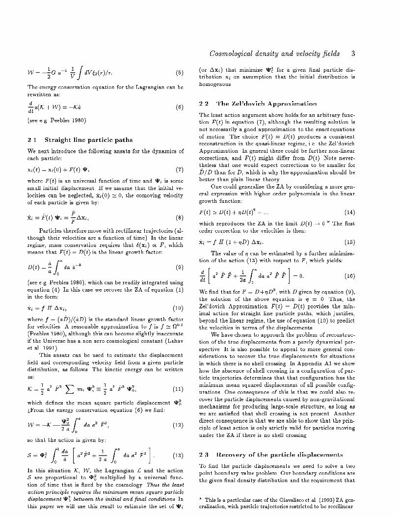
Figure 1. The action minimisation procedure carried out on an example two dimensional particle arrangement. In each panel the initial

particle positions are shown by open circles and the �nal positions by closed points. A solid line shows the path from each �nal position

to its currently selected initial position. In (a) we show the initial (randomly chosen) arrangement of paths. In (b) and (c) we show an

interchange of paths that is accepted by the procedure because it leads to a reduction in the action. Panel (d) shows the end state of the

system once it has \cooled".

the initial density is homogenous and peculiar velocities are

zero (Peebles 1989). We have already found the solution to

this problem in equation (13): the mean squared displace-

ment

2

0

must be minimised. As we have restricted ourselves

to straight line paths, the situation is particularly simple.

We �rst choose a homogenous distribution for the initial

particle positions. Here we use a cartesian grid, but other

types of sub-random distribution such as a glass (Baugh,

Gazta~naga and Efstathiou 1995) could also be used. The

situation now facing us is similar to that in the Travelling

Salesperson problem, where the object is to join up a list of

points with the shortest possible path. The situation here is

much simpler though as each

i

or segment of the path is

independent of all the others.

To �nd the displacements, we �rst assign a �nal particle

position to each initial position, at random. The displace-

ment vector

i

for each particle is given by the separation

between the �nal and allocated initial position, while the

action is proportional to the sum of the magnitudes of the

displacements squared. The initial situation for an illustra-

tive two dimensional density �eld is shown in Figure 1(a).

We carry out our minimisation procedure by picking pairs

of particles and interchanging their end points. If the result

leads to the sum of the path lengths squared being smaller,

the swap is accepted. This is shown in panels (b) and (c) of

Figure 1. Particle paths are interchanged in this way until

we decide to stop. We can base the decision of when to stop

on the behaviour of the action. In panel (d) of Figure 1 we

show the choice of particle trajectories for which the action

reached a satisfactory minimum in the example case.

There are some similarities between this method and

the method of simulated annealing (see e.g. Press et al. 1992)

which is one way of solving the Travelling Salesperson prob-

lem. In that problem, it is necessary to accept some path

swaps which increase the total length, as the path segments

are not independent. If the path length is longer, whether

the result is accepted depends on an arti�cial \temperature"

for the system. This temperature is slowly reduced according

to an annealing schedule so that decisions that involve large

scales are made �rst and then, as the system \cools", �ner

adjustments are made to the path until convergence to a

satisfactory approximation to the exact solution is reached.

In our case,simulated annealing is not necessary and we can

simply reject path swaps that result in an increase in the ac-

tion. Our approach can therefore be described as \simulated

quenching", and is free of the complications involving choice

of the annealing schedule which attend simulated annealing.

3 TESTS ON SIMULATIONS

To check the accuracy and range of validity of our Path

Interchange Zel'dovich Approximation (hereafter PIZA)

method we have carried out some tests using particle spa-

tial distributions and velocities taken from cosmological N-

body simulations. In most of our tests in this paper we will

deal with the idealised case of full sampling and periodic

boundary conditions. Various applications of our method

are checked in Sections 3.2 to 3.7.

3.1 Simulations used

We use simulations of two di�erent spatially at cold dark

matter dominated Universes. One simulation is of \stan-

dard" CDM, with

0

= 1; h = 0:5, and the other is of low

density CDM with

0

= 0:2; h = 1 and a cosmological con-

stant � = 0:8 � 3H

2

0

. The power spectra for each model

were taken from Bond & Efstathiou (1984) and Efstathiou,

Bond and White (1992). Each simulation contains 10

6

par-

ticles in a box of comoving side-length 30000 kms

�1y

and

y

Throughout the paper we use H

0

= 100h km s

�1

Mpc

�1

and

quote distances in units of H

�1

0

, i.e. in km=s.

Cosmological density and velocity �elds 5

Figure 2. The evolution of various quantities during the action

minimisation procedure. The horizontal axis corresponds to the

number of interchange trials divided by the total number of par-

ticles. In panel (a) we show show how the mean squared displace-

ment

2

0

(proportional to the action) changes. In panel (b) we

plot the fraction of interchange attempts which are accepted. In

panel (c) we plot the rms error on individual particle velocities

divided by the dynamical factor f . In each case the solid and dot-

ted lines correspond to the 30000 kms

�1

and 15000 kms

�1

box

standard CDM simulations. The dashed line show the results for

the 30000 kms

�1

box low density CDM model.

was run using a P

3

M N -body code (Hockney and Eastwood

1981, Efstathiou et al. 1985). The mean comoving interpar-

ticle separation is therefore 300 kms

�1

, of the same order

as that of normal galaxies. The simulations are descibed in

more detail in Croft and Efstathiou's (1994) study of galaxy

cluster clustering . In order to quantify the e�ects of particle

resolution, we have also run one additional standard CDM

simulation, also with 10

6

particles, but in a box of side length

15000 kms

�1

. This was also run with the P

3

M code, kindly

provided by G. Efstathiou. All the simulations used in Sec-

tions 3.2 to 3.6 have been evolved until the linear variance

(�

2

8

) of density in spheres of radius 800 kms

�1

= 8 h

�1

Mpc

is equal to 1.

3.2 Minimisation of the action

We carry out the procedure outlined in Section 2.3 on each

simulation, but with one additional re�nement. As the size

of the box is much larger than the expected maximum dis-

placement of a particle, we speed up the algorithm, by lim-

iting the interchange of particle paths to particles that are

within a certain distance r

max

. Our implementation of this

idea is as follows.

(a) We �rst pick at random a �nal particle i which is at

position x

i

.

(b) We then choose, also at random one of the initial grid

positions, x

j

(0), that is within r

max

of x

i

.

(c) We then assign this initial position x

j

(0) to particle i

and make x

i

(0) the initial position of particle j.

(d) If the sum of the path lengths squared for the new con�g-

uration is smaller than for the old, we accept the interchange

and assign new labels to the initial positions, otherwise we

keep the old con�guration.

(e) We then return to step (a) to carry out the procedure

on two more particl.es.

In order to �nd out when the system has reached a

satisfactory state and we can stop repeating this process, we

examine the behaviour of the mean squared displacement,

2

0

. In our tests we take the value of r

max

to be 2000 kms

�1

,

unless stated otherwise. In panel (a) of Figure 2 we show how

2

0

decreases as the number of particle interchange attempts

is increased. We plot results for all three of the simulations

described in Section 3.1. We can see that the low density

CDM model appears to be \cooling" slightly more slowly

than standard CDM with the same box size and reaches a

�nal state which has a higher value of

2

0

. This is probably

due to the fact that the low density model has more power

on large scales. This means that large scale bulk ows add to

the particles' average displacement. The small box standard

CDM simulation reaches an even lower value of

2

0

due to

the absence of large-scale modes. This simulation also cools

more slowly, as there are 8 times as many particles to choose

from within r

max

compared to the other two simulations.

In Figure 2 (b) we plot the fraction of pair interchange

attempts that are successful. We can see that the slope of the

curve changes slightly when

2

0

in panel (a) starts to level o�.

Panel (c) shows that we can safely assume the system has

reached a satisfactory solution when

2

0

levels o�. Here we

plot the rms error on individual predicted particle velocities

from our PIZA process, i.e. equation (10), against their true

values in the simulations. To compare di�erent curves, we

have divided them by the dynamical factor f = f(;�). We

�nd that 500 times the number of particles is an adequate

choice for the number of interchange attempts and this is

the number we will use unless stated otherwise.

Our procedure is about an order of magnitude slower

than competing Eulerian based systems such as the method

of Nusser and Dekel (1992), although it is surprisingly fast

given that it uses a technique related to simulated annealing.

We have carried out our computations using an SGI Chal-

lenge computer and DEC Alpha AXP 3000 workstations,

each minimisation taking 4� 8 cpu-hours.

6 R.A.C. Croft and E. Gazta~naga

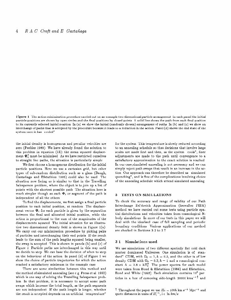
Figure 3. Recovery of the x component of particle displacements

(panels (a) and (b)) and the smoothed displacement �eld (panels

(d) and (d)) for the large box, StandardCDM simulation.The left

hand panels show the case for one PIZA particle per simulation

and in the right hand panels the predicted displacement has been

obtained by an average of 8 particles (see text). In panel (a) we

have added random scatter distributed like a top hat of width

20 kms

�1

to the x and y coordinates, so that the relative number

of points in each band can be seen.

3.3 Prediction of displacements

Once a reasonable approximation to the minimum action

solution to the particle displacments has been reached, we

can compare our results directly to the correct values from

the simulations. In Figure 3 we plot the x components of

displacements found using PIZA against the simulation val-

ues, for the case of the large box standard CDM simulation.

In this section and in section 3.4, we will carry out our com-

parisons on quantities evaluated at the �nal positions of the

particles.

Panel (a) shows the values for a random sample of 10

4

individual particles. We can see that the scatter between

values is large but there is also a de�nite correlation. More

obvious is the fact that the displacements are quantised due

to the initial con�guration being a grid. After arriving at the

individual displacements, we carry out a comparison with

the smoothed displacement �eld. We interpolate the den-

sity onto a 128

3

grid using a Triangle-Shaped Clouds (TSC)

scheme (see Hockney and Eastwood 1981). We then also in-

terpolate the displacement for each particle times its mass

(taken to be 1) onto a grid. We smooth both �elds in Fourier

space with a Gaussian �lter and divide the �rst �eld by the

second. The values of the x-component of this displacement

�eld at 10

4

randomly chosen grid points are plotted in Fig-

ure 3(c). We have used a smoothing length of 500 kms

�1

.

The e�ect of smoothing is to signi�cantly reduce the scat-

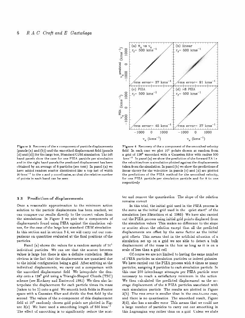
Figure 4. Recovery of the x component of the smoothed velocity

�eld. In each case we plot 10

4

points chosen at random from

a grid of 128

3

smoothed with a Gaussian �lter with radius 500

kms

�1

. In panel (a) we show the prediction of the forward ZA i.e.

the velocities from a simulation plotted against the displacements

taken from the simulation. In panel (b) we show the predictions of

linear theory for the velocities. In panels (c) and (d) are plotted

the predictions of the PIZA method for the smoothed velocity,

for one PIZA particle per simulation particle and for 8 to one

respectively.

ter and remove the quantisation. The slope of the relation

remains correct.

In this trial, the initial grid used in the PIZA process is

the same as the initial grid used in the \quiet start" of the

simulation (see Efstathiou et al. 1985). We have also carried

out the PIZA process using initial grid points displaced from

the simulation values. This makes no di�erence to the slope

or scatter about the relation except that all the predicted

displacements are o�set by the same factor as the initial

grid o�sets. This means that in the arti�cial situation of a

simulation set up on a grid we are able to detect a bulk

displacement of the mass in the box as long as it is on a

scale of less than a grid cell.

Of course we are not limited to having the same number

of PIZA particles as simulation particles or indeed galaxies.

We have carried out the PIZA process with 8 times as many

particles, assigning 8 particles to each simulation particle. In

this case 200 interchange attempts per PIZA particle were

necessary to reach a satisfactory minimum in the action.

We then calculated the predicted displacement as the av-

erage displacement of the 8 PIZA particles associated with

each simulation particle. The results are plotted in Figure

3(b). The rms error is smaller than in the one-to-one case,

and there is no quantisation. The smoothed result, Figure

3(d), also has a smaller error. This means that we could use

a large number of particles to carry out our smoothing in

this Lagrangian way rather than on a grid. Unless we state

Cosmological density and velocity �elds 7

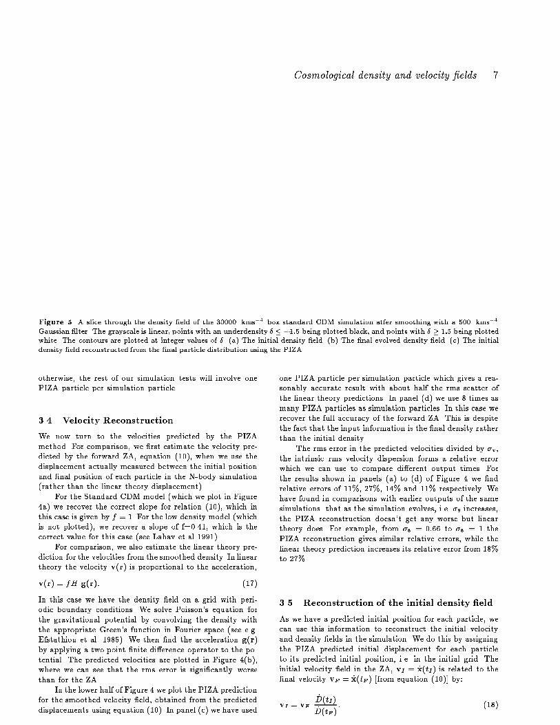
Figure 5. A slice through the density �eld of the 30000 kms

�1

box standard CDM simulation atfer smoothing with a 500 kms

�1

Gaussian �lter. The grayscale is linear, points with an underdensity � � �1:5 being plotted black, and points with � � 1:5 being plotted

white. The contours are plotted at integer values of �. (a) The initial density �eld. (b) The �nal evolved density �eld. (c) The initial

density �eld reconstructed from the �nal particle distribution using the PIZA.

otherwise, the rest of our simulation tests will involve one

PIZA particle per simulation particle.

3.4 Velocity Reconstruction

We now turn to the velocities predicted by the PIZA

method. For comparison, we �rst estimate the velocity pre-

dicted by the forward ZA, equation (10), when we use the

displacement actually measured between the initial position

and �nal position of each particle in the N-body simulation

(rather than the linear theory displacement).

For the Standard CDM model (which we plot in Figure

4a) we recover the correct slope for relation (10), which in

this case is given by f = 1. For the low density model (which

is not plotted), we recover a slope of f=0.41, which is the

correct value for this case (see Lahav et al 1991).

For comparison, we also estimate the linear theory pre-

diction for the velocities from the smoothed density. In linear

theory the velocity v(r) is proportional to the acceleration,

v(r) = fH g(r): (17)

In this case we have the density �eld on a grid with peri-

odic boundary conditions. We solve Poisson's equation for

the gravitational potential by convolving the density with

the appropriate Green's function in Fourier space (see e.g.

Efstathiou et al. 1985). We then �nd the acceleration g(r)

by applying a two point �nite di�erence operator to the po-

tential. The predicted velocities are plotted in Figure 4(b),

where we can see that the rms error is signi�cantly worse

than for the ZA.

In the lower half of Figure 4 we plot the PIZA prediction

for the smoothed velocity �eld, obtained from the predicted

displacements using equation (10). In panel (c) we have used

one PIZA particle per simulation particle which gives a rea-

sonably accurate result with about half the rms scatter of

the linear theory predictions. In panel (d) we use 8 times as

many PIZA particles as simulation particles. In this case we

recover the full accuracy of the forward ZA. This is despite

the fact that the input information is the �nal density rather

than the initial density.

The rms error in the predicted velocities divided by �

v

,

the intrinsic rms velocity dispersion forms a relative error

which we can use to compare di�erent output times. For

the results shown in panels (a) to (d) of Figure 4 we �nd

relative errors of 11%, 27%, 14% and 11% respectively. We

have found in comparisons with earlier outputs of the same

simulations. that as the simulation evolves, i.e. �

8

increases,

the PIZA reconstruction doesn't get any worse but linear

theory does. For example, from �

8

= 0:66 to �

8

= 1 the

PIZA reconstruction gives similar relative errors, while the

linear theory prediction increases its relative error from 18%

to 27%.

3.5 Reconstruction of the initial density �eld

As we have a predicted initial position for each particle, we

can use this information to reconstruct the initial velocity

and density �elds in the simulation. We do this by assigning

the PIZA predicted initial displacement for each particle

to its predicted initial position, i.e. in the initial grid. The

initial velocity �eld in the ZA, v

I

=_x(t

I

) is related to the

�nal velocity v

F

=_x(t

F

) [from equation (10)] by:

v

I

= v

F

_

D(t

I

)

_

D(t

F

)

: (18)

8 R.A.C. Croft and E. Gazta~naga

Figure 6. Scatter plots of the real initial density from standard CDM simulations plotted against the reconstructed initial density using

the PIZA (panels (a) to (c)) and linear theory (panels (d) to (f)). Three di�erent smoothing Gaussian lengths have been used (the values

of r

f

are given in each panel) and 10

4

points taken at random from a 128

3

grid are shown. The large box simulation was used for the

left hand four plots and the 15000 kms

�1

box simulation for the other two.

In this section, we are interested in testing the recon-

struction of the initial density �eld, for which we only need

to use the displacements. We assign the displacements to

a 128

3

cartesian grid as before using the TSC scheme and

smooth with a Gaussian �lter. The initial density �eld now

follows from the continuity relation:

�

I

(x

i

) = �D(t) r �

i

= �r � (�x

i

) (19)

In Figure 5 we plot a contour plot of a slice through the

smoothed density �eld in the large box standard CDM sim-

ulation. The Gaussian �lter used in the smoothing process

is of width 500 kms

�1

. The real initial density �eld used at

the start of the simulation (smoothed for the plot) is shown

in the left-hand panel. The amplitude of all �elds has been

scaled by a factor (1+z) in these comparison plots. Being a

Gaussian random �eld, this initial �eld has symmetry be-

tween the high and low density regions. Regions above a

threshold �

t

are statistically equivalent to regions below ��

t

.

The �nal, evolved density �eld (also smoothed) is shown

in the centre panel. This plot also corresponds to the linear

theory prediction for the initial density �eld (as we are using

the [1+z] scaling). Even though the �eld has been smoothed,

we can see the �lamentary distribution that results from

gravitational instability. The symmetry between high and

low density regions has now been broken. Voids have grown

in size and matter has aggregated into clusters, sheets and

�laments with a high relative overdensity.

In the right hand panel of Figure 5 we show the relevant

slice through the PIZA reconstruction of the initial density

�eld. The �eld bears a reasonable resemblance to the real

initial density �eld of panel (a), with the agreement being

best on large scales. The voids have shrunk compared to the

�nal conditions, and the small scale features now appear

closer to those in the initial density. Di�erences between

the real and reconstructed initial density �elds consist of a

general lack of de�nition on small scales and the fact that

the voids are not empty enough in the reconstruction. Both

of these e�ects are characteristic of using the ZA, although,

as with the forward ZA, many features of the density �eld

that do result from quasi-linear processes are surprisingly

well captured.

In Figure 6 we show a point by point comparison of the

smoothed density �elds. We use three di�erent �lters, going

from large to small scales from left to right. In panel (c)

we have used the higher resolution standard CDM simula-

tion in order to make a comparison using a 250 kms

�1

�lter.

In all the plots, the initial density is plotted on the x-axis

(again scaled by [1+z]). The �nal density (corresponding to

the linear theory prediction for the initial density) is plotted

on the y-axis for the lower three panels and the PIZA recon-

structed initial density on the upper three panels. We can

again see that using the PIZA method o�ers a substantial

improvement over linear theory. We return to a discussion

of the merits and accuracy of the PIZA compared to other

reconstruction methods in Section 4.

3.6 Reconstruction in redshift space

We can also carry out the PIZA reconstruction from the

redshift space coordinates of particles. If the observer is at

the origin, then for each particle, the redshift space �nal

Cosmological density and velocity �elds 9

coordinate s

i

is given in terms of the real space coordinate

x

i

and velocity_x

i

:

s

i

= x

i

+ s

i

(

_x

i

H

� s

i

); (20)

where s

i

= s

i

=js

i

j is the unit line of sight vector and H the

Hubble constant. Thus, in terms of the initial coordinate

x

i

(0), and displacement �x

i

we have:

s

i

= x

i

(0) + �x

i

+ s

i

(f�x

i

� s

i

): (21)

This linear set of equations can be trivially solved to obtain

the three components of the displacements �x

i

in terms

of the redshift and initial positions. This is all we need to

carry out the PIZA reconstruction, although the results will

depend on the value we assume for f .

To test the recovery of real space density from redshift

space, we have taken the large box standard CDM simula-

tion and added the particle's x-velocities to their x positions.

In this way, as we are using the x-axis as the line of sight

(the distant observer approximation).

Before we apply the PIZA process to the particle distri-

bution, we must �rst deal with the \�ngers of God" caused

by virialised galaxy clusters. These objects are the result

of strongly non-linear gravitational collapse on small scales,

which we cannot hope to follow with the ZA. Here we use

the approach of Gramman, Cen & Gott (1994) in choosing

to collapse the �ngers along the line of sight. We employ a

friends-of-friends group�nder written and �rst used by Davis

et al. (1985), which joins together into groups particles sepa-

rated by less than a certain linking length. We have modi�ed

the group�nder so that the linking length is di�erent for sep-

arations parallel to and perpendicular to the line of sight. To

collapse the �ngers, we place all particles in a group at the

average redshift of the group particles. The linking lengths

are chosen by estimating the correlation function of the par-

ticles as a function of separation across and along the line

line of sight. For the correct linking lengths, the correlation

function should be approximately symmetric on small scales

(r < 5 h

�1

Mpc) (see Gramman et al 1994). Here we use

linking lengths of 0.15 and 1.5 times the mean interparticle

separation for distances across and along the line of sight

respectively.

We then carry out the reconstruction process on the red-

shift space particle distribution. The line-of-sight distance

between the initial and �nal positions in redshift space is

larger than in real space (twice as large if = 1). We there-

fore use a larger search distance r

max

= 4000 kms

�1

in the

direction parallel to the line of sight. If we assume a value

for f and hence , the PIZA process yields predicted dis-

placements and velocities for the particles. We then use the

predicted velocities to reconstruct the �nal real space den-

sity distribution. In principle, we could choose the correct

value of f by picking the value which reproduces the isotropy

of the real-space correlation function, this time on interme-

diate to large scales (r > 5 h

�1

Mpc). This would be one

way of using the ZA to recover from redshift space dis-

tortions of clustering (for another way see e.g. Fisher and

Nusser 1995). We will discuss this further in Section 4. In

the meantime, as we are using the standard CDM simula-

tion, we take f = 1.

We again assign the particles to a 128

3

grid using the

TSC scheme and then smooth the density with a Gaussian

Figure 7. Recovery of the real space �nal density from redshift

space �nal density in the 30000 kms

�1

box standard CDM simu-

lation. (a) and (c) show the redshift space density (y-axis) plot-

ted against real space density (x-axis). (b) and (d) show the re-

covered real space density using the PIZA predicted velocities

(y-axis) against the true real space density (x-axis). Two di�er-

ent Gaussian smoothing �lters were used, 1500 kms

�1

(top) and

1000 kms

�1

(bottom), and a random sample of 10

4

grid points

are plotted.

�lter. When this smoothing process is carried out, we make

sure that the �ngers of God are kept compressed and that

their predicted velocity is given by the average of the PIZA

velocities of the particles they contain. We have already seen

(in Figure 3a) that because of relatively large separation of

the particles, the scatter in velocities of individual particles

is rather large. This scatter in velocities will translate into

a blurring of the redshift space density reconstruction on

small scales. To improve the results, we could reduce the

scatter by using more particles. In order to keep matters

simple in this preliminary test, we instead use a �lter size

large enough to smooth over the small scale scatter.

In Figure 7 we show the results for two di�erent �lter

sizes, r

f

= 1500 kms

�1

(top panels) and r

f

= 1000 kms

�1

(bottom panels). In all the panels, the real space density is

plotted on the x-axis. In (a) and (c), we have plotted the

redshift space density from the simulation on the y-axis. In

(b) and (d) we have plotted the PIZA reconstructed �nal

real space density on the y-axis. We can see from panels (a)

and (c) that transformation into redshift space increases the

relative density contrast as well as introducing some scatter.

The PIZA reconstruction restores the correct slope, even in

regions with a density contrast � > 1:5, as well as reducing

10 R.A.C. Croft and E. Gazta~naga

Figure 8. Reconstuction of the initial density �eld in the

30000 kms

�1

box standard CDM simulation from redshift space.

On the x-axis we plot the smoothed initial density �eld in the

simulation and on the y-axis we plot the smoothed PIZA recon-

structed initial density �eld. The amplitude of both �elds has

been scaled by (1+z) and a random sample of 10

4

grid points is

plotted in each panel.

the scatter. As expected, the reconstruction works best af-

ter �ltering on large scales. If we just compress the �ngers of

God without carrying the reconstruction, we see only min-

imal improvement in the scatter, in line with the results of

Gramman, Cen & Gott (1994).

We have also carried out the recovery of real space den-

sity in the low density CDM simulation. Random virial ve-

locities are not as important in this model, and we are able

to recover the real space density with similar accuracy to the

standard CDM trial even without compressing the �ngers of

God.

Since the �nal real space density can be recovered fairly

well, at least when smoothed on large scales, we now test the

reconstruction of the initial density �eld from the redshift

space �nal density. After applying the PIZA process, we have

to correct the particle �nal positions into real space using

their predicted velocities. After this, the process is identical

to that detailed in Section 3.3. The initial density and the

recovered initial density for the standard CDM model (after

using �lters of sizes 1500 kms

�1

and 1000 kms

�1

) are shown

in Figure 8. Comparing Figure 8b and Figure 6a we can see

that the scatter in the reconstruction has increased by a

factor of � 2:5 with respect to the result obtained in real

space. The reconstruction is still reasonable, though, and

there may exist ways to reduce this error, which we will

discuss in Section 4.

3.7 Application to biased simulations

When we apply a dynamical scheme to galaxy redshift data

rather than to the mass taken directly from a simulation,

we must take into account that the large scale galaxy distri-

bution might not be good tracer of the mass. In dynamical

schemes based on linear theory, it is common to invoke the

linear biasing model for the relationship between galaxies

and mass. In this model, it is assumed that if the galaxy den-

sity constrast �

g

(x) is smoothed on su�ciently large scales

then the mass density contrast is given by �

m

(x) = �

g

(x)=b.

This model is probably reasonable on large scales (see e.g.

Bardeen et al. 1986, Kaufmann et al. 1995), and has been

extensively used (see e.g. Dekel & Rees 1987, Strauss et al.

1992, Fisher et al. 1994). In these studies, there is a de-

generacy between the bias parameter b and the dynamical

factor f in equation (10). If we wish to break this degen-

eracy, we need to examine the situation on smaller scales,

using dynamical schemes which are valid in the quasi-linear

regime. Unfortunately, on scales small enough that we ex-

pect non-linearity in the gravitational evolution of mass, we

should also expect to �nd non-linearity in the relationship

between galaxies and mass (see e.g. Fry & Gazta~naga 1993)

and maybe even scale dependent biasing (see Gazta~naga &

Frieman 1994, Weinberg 1995) . If the biasing process can be

approximated by a local transformation, �

g

= F [�

m

], then

in Eulerian schemes it is possible to use a model to map

the galaxy density to mass density before carrying out a

reconstruction.

With a particle-based scheme such as that presented

here, it is not obvious what we should do. For example,

if galaxies are more clustered than mass then we should

somehow add particles to the underdense regions. However

even in the case of linear biasing, there does not appear

to be any simple prescription for \de-biasing" the galaxy

distribution using particles.

To test the possible e�ects of biasing, we apply a pre-

scription to select a population of galaxy particles that have

di�erent clustering properties from the underlying mass. For

this test we use the standard CDM 30000 kms

�1

box simula-

tion and choose galaxy particles as follows. For each particle

we �nd the distance to the 20th nearest particle and then

calculate the overdensity inside a sphere of this radius. If the

resulting uctuation is above a certain critical value (in this

case 0.5) we add the particle to the list of galaxies. These

galaxy particles are preferentially selected in high density

regions and are more clustered than the underlying mass.

We also add a fraction (30%) of the non-peak particles to

the list of galaxies to make up for the fact that the �nite

resolution of the simulations means that power is missing

on small scales which might have conceivably caused a few

galaxies to be formed in less overdense regions. We use a

simulation output which has �

8

= 0:66 for the mass. When

we apply the biasing procedure we �nd 89

3

galaxy parti-

cles and the resulting distribution has a rms uctuation is

Cosmological density and velocity �elds 11

Figure 9. Recovery of the x component of the smoothed velocity

�eld from biased and unbiased simulations with �

8

= 0:66 for

the underlying mass and �

8

= 1:0 for the biased particles. In

each case we plot 10

4

points chosen at random from a grid of

128

3

smoothed with a Gaussian �lter with radius 500 kms

�1

.

The lefthand panels show the prediction for the velocity �eld

from PIZA (a) and linear theory (c) when applied to the biased

simulations. The prediction has been scaled by one over the linear

bias factor (b=1.5) in both these panels. Panel (b) shows the

PIZA prediction for the velocity of the unbiased simulation.

spheres of 8h

�1

Mpc of �

b

8

= 1:0. We de�ne a linear bias

factor, b as:

b �

�

b

8

(biased)

�

8

(mass)

; (22)

so that in this case we have b = 1:5.

We apply the PIZA method to this simulated galaxy

distribution in the same way that we have previously done

with the mass. We take the predicted velocities assigned

to a grid and smoothed with a Gaussian �lter as before

and compare them with the real smoothed velocities of the

galaxy particles. The results are shown in panel (a) of Figure

9 , where we have scaled the prediction with the inverse of

the linear bias factor b.

Unlike in the case of linear theory, it is not obvious

that the linear bias factor should apply when relating the

predicted and observed velocities. We do expect particles

to have to travel farther in the biased simulation, but it is

interesting that this results in recovery of the same slope as

linear theory.

We have also used linear theory to predict the velocities

from the accelerations of the biased particles. The results,

also scaled with b, are being shown in panel (c) of Figure 9.

We can see that the scatter from in the linear theory plot is

again worse than for the PIZA prediction (the rms percent-

age error is 26% as opposed to 18% for PIZA). This result

shows that our reconstruction method still has the poten-

tial of being more accurate than linear theory, even when

used on a biased density distribution. If we apply the PIZA

method to the unbiased distribution, i.e. with �

8

= 0:66,

we predict the velocity �eld with even more accuracy (the

rms percentage error is 14%). This is shown in Figure 9b.

If there were some way of \de-biasing" the galaxy distribu-

tion, this could done in conjunction with a least squares �t

to the velocity �eld. Unfortunately there does not seem to

be a simple way of doing this, at least with the PIZA.

4 DISCUSSION

As far as comparison with the Eulerian ZA reconstruction

methods is concerned, panel (a) and (b) of Figure 6 should

be compared with the bottom panels of Figures 2(a) and

2(b) in Nusser and Dekel (1992). Our formulation of the

ZA gives a substantial improvement over the Zel'dovich

Bernoulli reconstruction. The PIZA has similar accuracy to

the Zel'dovich continuity approach of Gramman (1993a,b);

this is reasonable as both approaches are based on the re-

quirement of mass conservation.

Other methods for initial density reconstruction (e.g.

those of Nusser and Dekel 1992 and Gramman 1993a)

tend to require that redshift density be converted into real

space density prior to the reconstruction, a process which

usually requires an iterative technique (see e.g. Gramman

et al. 1994). For the Gaussian-mapping process of Wein-

berg (1992), the fact that the slope in Figure 7a is not

1 does not matter, as it is the rank ordering of densities

which is important. The scatter seen about the relationship

will mean increased errors in the reconstruction though. As

we have shown in Section 3.6 the PIZA method can handle

redshift space density �elds directly. The method will need

some modi�cation to deal with observed samples of galaxies

with a selection function as the rocket e�ect (Kaiser 1987)

will a�ect the reconstructed �elds. For example, linear the-

ory could be used initially to recover the real space selectio

function.

In principle, we could also use the method to mea-

sure , as the correlation function of the reconstructed real

space density should be isotropic. Some tests of this idea are

needed, and it is uncertain how the potentially complex re-

lationship between galaxies and mass will a�ect the results.

One advantage of a dynamical reconstruction from redshift

space to �nd is that we would not need to use the small

angle approximation. This approximation (that the observer

is su�ciently distant that pair separations long the line of

sight are parallel) is usually used and may lead to system-

atic errors for redshift surveys with large sky coverage (see

e.g. Hamilton and Culhane 1995).

An additional advantage of our particle-based scheme is

the fact that it is numerically stable even though no smooth-

ing is used before it is applied. Eulerian schemes usually re-

quire the application of di�erential operators to the density

�eld, so that smoothing is required before starting the re-

construction. This is potentially problematic as smoothing

must (�rst at least) be carried out in redshift space, which

will mean an additional loss of information on small scales,

particularly if particle velocities are large. Also, the smooth-

ing and non-linear dynamical operators do not commute.

This means that a self-consistent treatment of smoothing

12 R.A.C. Croft and E. Gazta~naga

is not possible in general in Eulerian schemes, which there-

fore sometimes require the application of empirically derived

smoothing corrections to the �nal results.

5 SUMMARY AND CONCLUSIONS

If the trajectories of particles or uid elements are restricted

to be straight lines (as in the Zel'dovich Approximation)

then the principle of least action leads to the simple con-

straint that the sum of the path lengths squared is min-

imised. This fact can be used in conjunction with a numer-

ical scheme to recover the displacement �eld from a �nal

particle distribution. This scheme is both intuitively sim-

ple and easy to implement. We have carried out tests of the

scheme on N-body simulation outputs of CDM universes and

�nd that when reconstructing the velocity �eld the results

have the same relatively small errors as an application of the

forward ZA. It is therefore natural to consider the scheme

to be a numerical inversion of the Lagrangian ZA. Although

the scheme is particle based, it is possible to minimise the

action of several million particles. This means that it should

be possible to assign several particles to each galaxy when

using observational data in the form of galaxy redshift sur-

veys. We should therefore be able to treat galaxy merging in

a limited way, and in any case we have shown here that the

use of more than one particle per galaxy increases the accu-

racy of the reconstruction. Our scheme can work in redshift

space, and can also be used to recover the real space density

from redshift space density.

As with other reconstruction methods our uncertainty

as to the relationship between galaxies and mass is one of

the fundamental limits to the accuracy of results. A study

of dynamics and galaxy biasing on scales small enough to

have some non-linearity needs a tool that can follow the

gravitational evolution of the mass with reasonable accuracy

on these scales. This is true of the PIZA method, which we

have shown to be substantially more accurate than linear

theory.

Acknowledgements

We would like to thank George Efstathiou for supplying

us with a copy of the P

3

M code and group�nder. We also

thank the anonymous referee for useful comments and sug-

gestions. RACC is supported by NASA Astrophysical The-

ory Grants NAG5-2864 and NAG5-3111 and would like to

thank David Weinberg for useful discussions and comments

on the manuscript. EG thanks the Astrophysics group in

Oxford for their hospitality, and acknowledges support from

CSIC, DGICYT (Spain), project PB93-0035 and CIRIT

(Generalitat de Catalunya), grant GR94-8001.

REFERENCES

Bardeen, J. M., Bond, J. R., Kaiser, N., & Szalay, A. S.

1986, ApJ, , 304,15

Baugh, C.M., Gazta~naga, E., Efstathiou, G., 1995, MN-

RAS, 274,1044

Bond, J.R., Efstathiou, G., 1984, ApJ, , 285, L45

Babul A., Weinberg D.H., Dekel, A., Ostriker J.P., 1994,

ApJ, , 427, 1

Bouchet, F.R., Colombi, S., Hivon, E., Juszkiewicz, R., 1995,

A&A,296, 575

Burstein, D., 1990, Rep.Prog.Phys., 53, 421

Catelan, P., 1995, MNRAS, 276, 115

Coles, P., Melott, A.L., Shandarin, S. F., 1993, MNRAS, ,

260, 765

Croft, R.A.C., Efstathiou, G., 1994, MNRAS, , 267, 390

Davis, M., Efstathiou, G., Frenk, C.S., White, S.D.M., 1985,

ApJ, , 292, 371

Davis, M., Peebles, P.J.E., 1983, ApJ, 267, 465

Dekel, A., Rees, M.J., Nature, 326, 455

Dressler, A., Lynden-BEll, D., Burstein, D., Davis, R.L.,

Faber, S.M., Terlevich, R.J., Wegner, G., 1987, ApJ, ,

313, 42

Doroshkevich, A. G., Kotok, E. V., Novikov, I. D., Polyudov,

A. N., Shandarin, S. F., 1980, MNRAS, , 192, 321

Efstathiou, G., Bond, J.R., White, S.D.M., 1992, MNRAS,

, 258, 1p

Efstathiou, G., Davis, M., Frenk, C.S., White, S.D.M., 1985,

Astrophys. J. Suppl., 57, 241

Fisher, K.B., Nusser, A., 1995, preprint

Fisher, K.B., Davis, M., Strauss, M.A., Yahil, A., Huchra,

J., 1994, MNRAS, 266, 50

Fry, J.N., Gazta~naga, E., 1993, ApJ, 413, 447

Gazta~naga, E., Frieman, J.A., 1994, ApJ,437, L13

Giavalisco, M., Mancinelli, B., Mancinelli, P.J., Yahil, A.,

ApJ, , 411, 9

Gramann, M., 1993a, ApJ, , 405, 449

Gramann, M., 1993b, ApJ,, 405, L47

Gramman, M., Cen, R., Gott, J.R., 1994, 425, 382

Hamilton, A.J.S., Culhane, M., 1995, preprint

Hockney, R. W., Eastwood, J. W., 1981, Numerical simula-

tions using particles (New York: McGraw-Hill)

Kau�mann, G., Nusser, A., Steinmetz, M., 1995, preprint

Lahav, O., Lilje, P.B., Primack, J.R., Rees, M.J., 1991, MN-

RAS, , 251, 128

Lifshitz E.M., 1946, J.Phys.USSR, 10, 116

Moutarde F., Alimi J-M, Bouchet F.R., Pellat R., Ramani

A., 1991, ApJ, 382, 377

Nusser, A., Dekel, A., 1992, ApJ, , 391, 443

Peebles, P.J.E., 1980, The Large Scale Structure of the Uni-

verse: Princeton University Press

Peebles, P.J.E., 1989, ApJ,, 344, L53

Press, W.H., Teukolsky, S.A., Vetterling, W.T., Flannery

B.P., 1992, Numerical Recipes (Cambridge)

Sahni, V., Shandarin, S., 1995, preprint

Shaya, E. J., Peebles, P.J.E., Tully, R. B., 1995, ApJ, , 454,

15

Susperregi M.P., Binney, J.J., 1994, MNRAS, , 271, 719

Weinberg, D. H., 1992, MNRAS, , 254, 315

Weinberg, D. H., 1995, in Wide-Field Spectroscopy and the

Distant Universe, eds S.J. Maddox and A. Arag�on-

Salamanca, World Scienti�c, Singapore.

Willick, J., Courteau, S., Faber, S.M., Burstein, D., Dekel,

A. 1995, ApJ, , 446, 12

Zel'dovich, Ya B., 1970, A & A,5,84

Cosmological density and velocity �elds 13

APPENDIX A1: SHELL CROSSING AND

MINIMUM MEAN SQUARED DISPLACEMENT

It is possible that the con�guration of displacements d

i

which connects pairwise the initial r

i

(0) and �nal positions

r

i

could have a minimum mean squared value with respect

to any other possible pair con�guration, regardless of the

least action principle or the Zel'dovich approximation.

This is trivially the case when the displacements are very

small compared to the interparticle separation. To see this

we consider the set of all possible pair con�gurations,

fr

i

(0); s

i

g where s

i

= r

j

is given by a set of j = 1; ::; n

indices that are permutations of the i = 1; ::;n indices. Let

us call

2

T

=

P

d

2

i

the true mean square displacement. For

any other con�guration we have

2

�

P

i

(r

i

(0)�s

i

)

2

which

gives:

2

=

2

T

+ 2

X

i

d

i

(r

i

� s

i

) +

X

i

(r

i

� s

i

)

2

: (A1)

When the displacements are small, d

i

! 0, we have :

2

=

2

T

+

X

(r

i

� s

i

)

2

: (A2)

so that for any other con�guration

2

>

2

T

, and therefore

2

T

is the minimum of all possible con�gurations.

The above argument cannot be used in general when the

displacements d

i

are large. The term 2

P

d

i

(r

i

� s

i

) does

not vanish by isotropy because in general the con�guration

that minimizes

2

does not have to be isotropic with respect

to the true con�guration.

We will now show that when there is no shell crossing (nsc)

in the trajectories of a con�guration, its mean squared dis-

placement is the minimum of all possible pair con�gurations.

Let us �rst de�ne shell crossing (sc) and mean squared dis-

placement.

Definition 1. Given two trajectories connecting the position

r

i

(0) with r

i

and r

j

(0) with r

j

, we will say that there is shell

crossing between these trajectories whenever:

[r

i

� r

i

(0)]

2

+ [r

j

� r

j

(0)]

2

> [r

i

� r

j

(0)]

2

+ [r

j

� r

i

(0)]

2

: (A3)

That is, the total path of the actual trajectories is larger

than the path of the crossed trajectories, where we swap the

�nal (or initial) positions.

Definition 2.Given two sets of positions r

i

(0) with i = 1; :::n and

r

j

with j = 1; :::n, consider the group of all pair con�gurations

given by the set of all permutations of the index j, which we label

j

i

= fj

1

; ::; j

n

g. For each con�guration fj

i

g connecting positions

r

i

(0) with r

j

i

, we de�ne the mean square displacement

2

as:

2

�

1

n

X

i

[r

j

i

� r

i

(0)]

2

: (A4)

We can now prove the following theorem.

Theorem. A pair con�guration has a minimum mean square

displacement if and only if there is no shell crossing (nsc) in

this con�guration.

Let us label the one particular con�guration we are inter-

ested in by T

i

, with mean squared displacement:

2

T

. We can

formally express this theorem in the following notation:

nsc fT

i

g ()

2

T

�

2

8fj

i

g (A5)

This is equivalent to saying that there is shell crossing (sc)

in fT

i

g if and only if there is some con�guration fj

i

g with

2

for which

2

T

>

2

:

sc fT

i

g () 9fj

i

g

<

2

T

: (A6)

The proof of the theorem has therefore two steps. We �rst

prove that:

sc fT

i

g =) 9fj

i

g

<

2

T

: (A7)

This can be shown as follows. If we just swap (permute) the

pairs in the sum of

2

T

of fT

i

g where there is shell crossing,

it follows from the de�nition of sc that the permuted con�g-

uration will have a smaller value of

2

, and therefore (A7)

is true. We now show that the other direction holds also:

9fj

i

g

2

T

>

2

=) sc fT

i

g: (A8)

This can be shown as follows. Consider the con�guration

fj

i

g for which the above is true. Group arbitrarily the in-

dices i = 1; :::;n in pairs and call the members of each pair

fk1; k2g. We will have:

2

=

X

k1

[r

j

k1

� r

k1

(0)]

2

+ [r

j

k2

� r

k2

(0)]

2

(A9)

where j

k1

and j

k2

are the indices of the �nal positions as-

sociated with k1 and k2 in the con�guration fj

i

g, for which

2

<

2

T

. We do the same grouping for the fT

i

g con�g-

uration. As all terms above are positive and

2

<

2

T

, it

follows that there is at least one term in the sum above

which is smaller than the corresponding term in the sum for

the fT

i

g con�guration. That is, there is shell crossing for at

least the pair corresponding to this term and therefore (A8)

is true.

An immediate consequence of this theorem is that there are

many situations for which one can recover the displacements

(by looking for the minimum in

2

) and which might have

nothing to do with gravity or the Zel'dovich Approximation

(ZA). This is similar to the situation which occurs with the

relation � � rv which also applies to non-gravitational sys-

tems (Babul et al. 1995). In our case, however, it does not

apply to the velocities, which in general do not have to be

proportional to the displacements. If we decide arbitrarily

that they do, we would still have to appeal to gravitational

dynamics and the Zel'dovich Approximation for the propor-

tionality factor.

Another direct consequence is the following corollary

Corollary The least action principle for particles moving under

gravity in an expanding universe requires that there is no shell

crossing as long as particles move in straight lines (that is under

the ZA).

We have shown in section 2 that the con�guration which

results from application of the least action principle has the

minimum mean square displacement and therefore, under

the above Theorem this means that there is nsc. Another

way of saying this is that the ZA can only be valid as far as

there is nsc. The appeal of the approach we take in Section

2 is that for straight line paths we have both a dynami-

cal approach (ZA) and a reconstruction method (minimum

2

) which are consistent with each other and which yield

accurate results with large enough smoothing.