
ASTR565 StellarStructureandEvolution Fall2019 ...
156
1 ASTR 565 Stellar Structure and Evolution Fall 2019 New Mexico State University Jason Jackiewicz Department of Astronomy December 5, 2019
Transcript of ASTR565 StellarStructureandEvolution Fall2019 ...
1
ASTR 565
Stellar Structure and Evolution
Fall 2019
New Mexico State University
Jason Jackiewicz
Department of Astronomy
December 5, 2019

2
Contents
I Stellar Structure 7
1 Equilibrium and time scales 9
1.1 Energy equilibrium . . . . . . . . . . . . . . . . . . . . . . . . . . . . . . . . . . . . . . . . . . 9
1.2 Local thermodynamic equilibrium . . . . . . . . . . . . . . . . . . . . . . . . . . . . . . . . . . 10
1.3 Are stars a one-fluid plasma? . . . . . . . . . . . . . . . . . . . . . . . . . . . . . . . . . . . . 10
1.4 Simple time scales of stars . . . . . . . . . . . . . . . . . . . . . . . . . . . . . . . . . . . . . . 11
1.4.1 Dynamical timescale . . . . . . . . . . . . . . . . . . . . . . . . . . . . . . . . . . . . . 11
1.4.2 Thermal timescale . . . . . . . . . . . . . . . . . . . . . . . . . . . . . . . . . . . . . . 12
1.4.3 Nuclear timescale . . . . . . . . . . . . . . . . . . . . . . . . . . . . . . . . . . . . . . . 12
1.5 Problems . . . . . . . . . . . . . . . . . . . . . . . . . . . . . . . . . . . . . . . . . . . . . . . 12
2 Nuclear interactions 15
2.1 Coulomb barrier . . . . . . . . . . . . . . . . . . . . . . . . . . . . . . . . . . . . . . . . . . . 15
2.2 Nuclear reaction rates . . . . . . . . . . . . . . . . . . . . . . . . . . . . . . . . . . . . . . . . 15
2.3 Gamow peak . . . . . . . . . . . . . . . . . . . . . . . . . . . . . . . . . . . . . . . . . . . . . 17
2.4 Problems . . . . . . . . . . . . . . . . . . . . . . . . . . . . . . . . . . . . . . . . . . . . . . . 19
3 Energy release in nuclear reactions 21
3.1 Mass excess . . . . . . . . . . . . . . . . . . . . . . . . . . . . . . . . . . . . . . . . . . . . . . 21
3.2 Binding energy . . . . . . . . . . . . . . . . . . . . . . . . . . . . . . . . . . . . . . . . . . . . 22
3.3 Hydrogen burning . . . . . . . . . . . . . . . . . . . . . . . . . . . . . . . . . . . . . . . . . . 23
3.3.1 PP-I chain . . . . . . . . . . . . . . . . . . . . . . . . . . . . . . . . . . . . . . . . . . 24
3.3.2 PP-II and PP-III chains . . . . . . . . . . . . . . . . . . . . . . . . . . . . . . . . . . . 25
3.3.3 CNO cycle . . . . . . . . . . . . . . . . . . . . . . . . . . . . . . . . . . . . . . . . . . 26
3.4 Problems . . . . . . . . . . . . . . . . . . . . . . . . . . . . . . . . . . . . . . . . . . . . . . . 27
4 Distribution functions 29
4.1 An example . . . . . . . . . . . . . . . . . . . . . . . . . . . . . . . . . . . . . . . . . . . . . . 29
4.2 Partition function . . . . . . . . . . . . . . . . . . . . . . . . . . . . . . . . . . . . . . . . . . . 30
4.2.1 Distinguishable particles . . . . . . . . . . . . . . . . . . . . . . . . . . . . . . . . . . . 30
4.2.2 Identical fermions . . . . . . . . . . . . . . . . . . . . . . . . . . . . . . . . . . . . . . 30
4.2.3 Identical bosons . . . . . . . . . . . . . . . . . . . . . . . . . . . . . . . . . . . . . . . 31
4.3 Derivation . . . . . . . . . . . . . . . . . . . . . . . . . . . . . . . . . . . . . . . . . . . . . . . 31
5 Mean molecular weight 33
6 Equation of state: Ideal gas 37
6.1 Preliminaries . . . . . . . . . . . . . . . . . . . . . . . . . . . . . . . . . . . . . . . . . . . . . 37
6.2 Maxwell-Boltzmann statistics . . . . . . . . . . . . . . . . . . . . . . . . . . . . . . . . . . . . 38
6.3 Ideal monatomic gas . . . . . . . . . . . . . . . . . . . . . . . . . . . . . . . . . . . . . . . . . 39
3
4 CONTENTS
7 Equation of state: Degenerate gas 41
7.1 Completely degenerate gas . . . . . . . . . . . . . . . . . . . . . . . . . . . . . . . . . . . . . . 417.2 Partially degenerate gas . . . . . . . . . . . . . . . . . . . . . . . . . . . . . . . . . . . . . . . 44
8 Density-temperature equation of state landscape 45
8.1 Radiation pressure . . . . . . . . . . . . . . . . . . . . . . . . . . . . . . . . . . . . . . . . . . 458.2 Putting it all together . . . . . . . . . . . . . . . . . . . . . . . . . . . . . . . . . . . . . . . . 46
9 Hydrostatic Equilibrium 49
9.1 Derivation . . . . . . . . . . . . . . . . . . . . . . . . . . . . . . . . . . . . . . . . . . . . . . . 499.2 Simple solutions . . . . . . . . . . . . . . . . . . . . . . . . . . . . . . . . . . . . . . . . . . . 52
9.2.1 Linearized density . . . . . . . . . . . . . . . . . . . . . . . . . . . . . . . . . . . . . . 529.2.2 Isothermal atmosphere . . . . . . . . . . . . . . . . . . . . . . . . . . . . . . . . . . . . 52
10 Polytropes 53
10.1 Motivation and derivation . . . . . . . . . . . . . . . . . . . . . . . . . . . . . . . . . . . . . . 5310.2 Lane-Emden equation . . . . . . . . . . . . . . . . . . . . . . . . . . . . . . . . . . . . . . . . 5410.3 Polytrope solutions . . . . . . . . . . . . . . . . . . . . . . . . . . . . . . . . . . . . . . . . . . 5510.4 Usefulness of polytropes . . . . . . . . . . . . . . . . . . . . . . . . . . . . . . . . . . . . . . . 58
11 Thermodynamics of an Ideal Gas 63
11.1 First law of thermodynamics . . . . . . . . . . . . . . . . . . . . . . . . . . . . . . . . . . . . 6311.2 Adiabatic process . . . . . . . . . . . . . . . . . . . . . . . . . . . . . . . . . . . . . . . . . . . 64
12 Thermodynamics with Photons 67
12.1 Mixture of ideal gas and radiation: pressure effects . . . . . . . . . . . . . . . . . . . . . . . . 6712.2 Mixture of ideal gas and radiation: ionization effects . . . . . . . . . . . . . . . . . . . . . . . 6912.3 Useful ideal gas equations . . . . . . . . . . . . . . . . . . . . . . . . . . . . . . . . . . . . . . 72
13 Energy Transport: Radiation 73
13.1 Basics . . . . . . . . . . . . . . . . . . . . . . . . . . . . . . . . . . . . . . . . . . . . . . . . . 7313.2 Diffusion . . . . . . . . . . . . . . . . . . . . . . . . . . . . . . . . . . . . . . . . . . . . . . . . 7413.3 Frequency dependence of radiation . . . . . . . . . . . . . . . . . . . . . . . . . . . . . . . . . 75
14 Opacity sources 77
14.1 Kramer’s Laws . . . . . . . . . . . . . . . . . . . . . . . . . . . . . . . . . . . . . . . . . . . . 7714.2 Consequences . . . . . . . . . . . . . . . . . . . . . . . . . . . . . . . . . . . . . . . . . . . . . 79
15 Convection 83
15.1 Temperature gradients (“dels”) . . . . . . . . . . . . . . . . . . . . . . . . . . . . . . . . . . . 8315.2 The convective instability . . . . . . . . . . . . . . . . . . . . . . . . . . . . . . . . . . . . . . 84
16 Convection 2 87
16.1 Other formulations of the instability . . . . . . . . . . . . . . . . . . . . . . . . . . . . . . . . 8716.2 Physical conditions for convection onset . . . . . . . . . . . . . . . . . . . . . . . . . . . . . . 8816.3 Depth of outer convection zones . . . . . . . . . . . . . . . . . . . . . . . . . . . . . . . . . . . 8916.4 Semiconvection . . . . . . . . . . . . . . . . . . . . . . . . . . . . . . . . . . . . . . . . . . . . 8916.5 Mixing length theory . . . . . . . . . . . . . . . . . . . . . . . . . . . . . . . . . . . . . . . . . 9116.6 Convective overshoot . . . . . . . . . . . . . . . . . . . . . . . . . . . . . . . . . . . . . . . . . 9316.7 An entropy formulation . . . . . . . . . . . . . . . . . . . . . . . . . . . . . . . . . . . . . . . 9316.8 An energy formulation . . . . . . . . . . . . . . . . . . . . . . . . . . . . . . . . . . . . . . . . 93
II Stellar Evolution 97
17 Overview of Asteroseismology 99
CONTENTS 5
18 Theory of the Main Sequence 101
18.1 Summary of stellar structure . . . . . . . . . . . . . . . . . . . . . . . . . . . . . . . . . . . . 101
18.2 Homology relations for stars in radiative equilibrium . . . . . . . . . . . . . . . . . . . . . . . 102
18.3 Dependence on mass . . . . . . . . . . . . . . . . . . . . . . . . . . . . . . . . . . . . . . . . . 103
19 Evolution on the main sequence 107
19.1 Low-mass stars . . . . . . . . . . . . . . . . . . . . . . . . . . . . . . . . . . . . . . . . . . . . 107
19.2 High-mass stars . . . . . . . . . . . . . . . . . . . . . . . . . . . . . . . . . . . . . . . . . . . . 108
19.3 Summary of main-sequence properties . . . . . . . . . . . . . . . . . . . . . . . . . . . . . . . 111
20 The Terminal-Age Main Sequence and Subgiant Branch 115
20.1 Description of evolution movies . . . . . . . . . . . . . . . . . . . . . . . . . . . . . . . . . . . 115
20.2 TAMS . . . . . . . . . . . . . . . . . . . . . . . . . . . . . . . . . . . . . . . . . . . . . . . . . 115
20.3 Schonberg-Chandrasekhar Limit . . . . . . . . . . . . . . . . . . . . . . . . . . . . . . . . . . 117
20.4 The subgiant branch . . . . . . . . . . . . . . . . . . . . . . . . . . . . . . . . . . . . . . . . . 119
21 Towards and up the Red-Giant Branch 121
21.1 High-mass stars . . . . . . . . . . . . . . . . . . . . . . . . . . . . . . . . . . . . . . . . . . . . 121
21.1.1 Low-mass stars . . . . . . . . . . . . . . . . . . . . . . . . . . . . . . . . . . . . . . . . 122
21.2 Helium flash . . . . . . . . . . . . . . . . . . . . . . . . . . . . . . . . . . . . . . . . . . . . . . 124
22 Red-Giant Branch Morphology 127
22.0.1 RGB properties . . . . . . . . . . . . . . . . . . . . . . . . . . . . . . . . . . . . . . . . 127
22.1 RGB location . . . . . . . . . . . . . . . . . . . . . . . . . . . . . . . . . . . . . . . . . . . . . 127
22.2 RGB bump luminosity . . . . . . . . . . . . . . . . . . . . . . . . . . . . . . . . . . . . . . . . 127
22.3 RGB tip luminosity . . . . . . . . . . . . . . . . . . . . . . . . . . . . . . . . . . . . . . . . . 128
23 The Horizontal Branch 131
23.1 Quick tour of non-hydrogen nuclear reactions . . . . . . . . . . . . . . . . . . . . . . . . . . . 131
23.2 The horizontal branch properties . . . . . . . . . . . . . . . . . . . . . . . . . . . . . . . . . . 132
23.3 Horizontal branch evolution . . . . . . . . . . . . . . . . . . . . . . . . . . . . . . . . . . . . . 133
23.3.1 High-mass stars . . . . . . . . . . . . . . . . . . . . . . . . . . . . . . . . . . . . . . . . 133
23.3.2 Low-mass stars . . . . . . . . . . . . . . . . . . . . . . . . . . . . . . . . . . . . . . . . 134
24 Asymptotic Giant Branch 137
24.1 General overview . . . . . . . . . . . . . . . . . . . . . . . . . . . . . . . . . . . . . . . . . . . 137
24.2 Double-shell burning . . . . . . . . . . . . . . . . . . . . . . . . . . . . . . . . . . . . . . . . . 137
24.3 AGB evolution . . . . . . . . . . . . . . . . . . . . . . . . . . . . . . . . . . . . . . . . . . . . 138
24.4 Thermal pulses . . . . . . . . . . . . . . . . . . . . . . . . . . . . . . . . . . . . . . . . . . . . 139
24.5 Production of s elements . . . . . . . . . . . . . . . . . . . . . . . . . . . . . . . . . . . . . . . 141
25 Last Stages of Evolution: Low-Mass Stars 143
25.1 Planetary Nebula . . . . . . . . . . . . . . . . . . . . . . . . . . . . . . . . . . . . . . . . . . . 143
25.2 White Dwarfs . . . . . . . . . . . . . . . . . . . . . . . . . . . . . . . . . . . . . . . . . . . . . 144
25.3 Futher WD properties . . . . . . . . . . . . . . . . . . . . . . . . . . . . . . . . . . . . . . . . 146
25.4 Type Ia supernovae . . . . . . . . . . . . . . . . . . . . . . . . . . . . . . . . . . . . . . . . . . 147
26 Last Stages of Evolution: High-Mass Stars 149
26.1 Nuclear burning . . . . . . . . . . . . . . . . . . . . . . . . . . . . . . . . . . . . . . . . . . . 149
26.2 Type II supernova - core collapse . . . . . . . . . . . . . . . . . . . . . . . . . . . . . . . . . . 150
26.3 Neutron star . . . . . . . . . . . . . . . . . . . . . . . . . . . . . . . . . . . . . . . . . . . . . 152
26.4 Black hole . . . . . . . . . . . . . . . . . . . . . . . . . . . . . . . . . . . . . . . . . . . . . . . 152

6 CONTENTS
27 Instability Strip and Pulsations 153
27.1 Background . . . . . . . . . . . . . . . . . . . . . . . . . . . . . . . . . . . . . . . . . . . . . . 15327.2 Pulsation mechanisms . . . . . . . . . . . . . . . . . . . . . . . . . . . . . . . . . . . . . . . . 15427.3 Ionization zones . . . . . . . . . . . . . . . . . . . . . . . . . . . . . . . . . . . . . . . . . . . . 156
Appendix A Conduction 157
A.1 Eddington Luminosity . . . . . . . . . . . . . . . . . . . . . . . . . . . . . . . . . . . . . . . . 157A.2 Conduction . . . . . . . . . . . . . . . . . . . . . . . . . . . . . . . . . . . . . . . . . . . . . . 158
Appendix B The Virial Theorem 159
Bibliography 163
Part I
Stellar Structure
7


Unit 1
Equilibrium and time scales
1.1 Energy equilibrium
• Consider a thin layer at location r and of width dr in the nuclear burning region of a star. For energyequilibrium, the net flow of energy crossing this region’s boundaries should be equal to the energygeneration in the region.
• Let ε be the energy generated per gram of material per second, so the energy generated per second in(r, dr) is εdm.
• Consider the luminosity (energy per second) L that carries energy away. In the layer, there shouldbe a balance between energy gains and energy losses (plus and minus denotes outgoing from center ortoward center, respectively):
εdm + L+r + L−
r+dr = L−r + L+
r+dr (1.1)
εdm = [L+r+dr − L−
r+dr]− [L+r − L−
r ] = Lr+dr − Lr (1.2)
εdm/dr = dL/dr, (1.3)
by dividing by dr and letting it go to zero (derivative).
• This standard relation will appear many times:
ρ =dm
dV, (1.4)
or,dm = 4πr2ρ dr (1.5)
• If ρ ε is the energy produced per second in each cm3 of material, then by unit analysis the energygenerated per second in (r, dr) is also given by
εdm = (4πr2dr)ρε. (1.6)
• Therefore, we can finally statedL
dr= 4πr2ρ ε. (1.7)
• Sometimes we will use m instead of r as the independent coordinate, and so
dL
dm= ε. (1.8)
9

10 UNIT 1. EQUILIBRIUM AND TIME SCALES
• This is one of the main equations of stellar structure.
• Note that in regions where ε = 0, the luminosity is constant.
• The properties of ε, its temperature dependence and derivation, are discussed in Unit 3.
• See Problem 1.1.
1.2 Local thermodynamic equilibrium
• Collisions between particles in a gas and/or radiation allow equilibrium to occur if the distance particlestravel and the time between collisions is small compared to macroscopic length and time scales.
• If this condition is met by radiation, it is known as blackbody radiation and the gas and radiation fieldare at the same temperature locally.
• This is known as local thermodynamic equilibrium (LTE).
• Specifically, the mean free path of photons is given by
ℓ =1
κρ, (1.9)
where κ is the opacity and ρ is density.
• We’ll see later that for a fully ionized gas that electron scattering gives κ = 0.4 cm2 g−1.
• Even for an average stellar density of ρ = 1.4 g cm−3, the mean free path of photons is about 1 cm.Lots of collisions.
• In stellar interiors this is almost always the case. Above stellar photospheres this assumption breaksdown.
• For example, the radiation leaving the Sun’s surface is at about 6,000K. However, the gas (electron)temperature of the corona, through which this radiation passes, can be over 1,000,000K. The matterand radiation have not equilibrated. This is actually an outstanding problem.
• On the other end, the 6000K radiation from the Sun passes through Earth’s 300K atmosphere alsowithout (thankfully) equilibrating.
• In any case, assuming LTE allows us to calculate the interior structure of a star and all the thermo-dynamic properties in terms of temperature, density, and composition. This is done at each radiallocation, and as a function of time.
1.3 Are stars a one-fluid plasma?
• We know stars are mostly ionized. Shouldn’t we treat the positive and negative charges as separately?
• If collisions are sufficiently frequent and Maxwellian and have times scales much less than other timescales of interest, then we can use a one-fluid model and generally ignore charge separation.
• The Debye length is the length over which an appreciable electric field can arise. It is roughly a measureof the thermal energy/electric potential energy ratio. If this length is short with respect to the plasma,we can assume charge neutrality.
λD =
√
ǫ0kBTe
neq2e≈ 6.9
(
Te
ne
)1/2
× 10 m (1.10)

1.4. SIMPLE TIME SCALES OF STARS 11
• In the core of the Sun, ne = 1032 m−3 and Te = 107K, so that λD ≈ 10−11 m. In the photosphere,ne = 1011 m−3 and Te = 5 × 10³ K, so that λD ≈ 1.5 × 10⁻³ m. For the corona, we may find thatλD ≈ 10 m.
• So the mean free path of ions (electrons) are much smaller than the scale of the variations of phys-ical quantities. Therefore we can treat most regions of stars as a one-fluid plasma system and usehydrodynamics. In coronae, however, it may be necessary to resort to plasma physics where manyapproximations are no longer valid.
1.4 Simple time scales of stars
While stars are for the most part static or quasistatic, and in equilibrium, there are time scales over whichchange may occur on a global scale. We can consider some quantity, say φ, and its rate of change φ = dφ/dt.Any relevant time scale is thus φ/φ.
1.4.1 Dynamical timescale
• Let’s first consider the smallest (and most observable) timescale tdyn.
• Consider a change in the fundamental dimension of the star, its radius φ = R, may be possible toexamine.
• Since gravity is the binding force, the velocity in a gravitational field is the escape velocity φ =(2GM/R)−1/2.
• Then (neglecting factors of order unity),
tdyn =
(
R3
GM
)1/2
. (1.11)
Note that in terms of the mean density of a star tdyn ≈ (Gρ)−1/2.
• In terms of solar values, we find
tdyn ≈ 30min
(
R
R⊙
)3/2(M
M⊙
)−1/2
. (1.12)
So since we don’t see large-scale changes on such time scales, we know there must be some balance offorces in the Sun. See Problem 1.2.
• Another way of thinking about this is to start with
g =GM
R2. (1.13)
• The time for a particle to fall under gravity is ℓ = 1/2gt2 → t =√
2ℓ/g. The time scale therefore fora particle to fall, say, a distance ℓ = R/2 in a star is
tdyn =
(
R3
GM
)1/2
, (1.14)
which reproduces Eq. (1.11).
• Dynamical processes in stars that help it adjust out of hydrostatic equilibrium typically occur overdynamical timescales, such as oscillations and even supernovae.
12 UNIT 1. EQUILIBRIUM AND TIME SCALES
1.4.2 Thermal timescale
• There exist thermal processes that affect the internal energy of a star, which we’ll denote as φ = U .
• As we’ll see from the Virial Theorem, U ≈ GM2/R.
• The energy changes due to radiation, whose rate of change is the luminosity φ = L.
• If we consider that losing its gravitational potential energy is the only real source of energy, then wecan calculate the time a star can radiate at a given luminosity. This is the Kelvin-Helmholtz timescaleand can be shown to be:
tKH ≈ 30Myr
(
M
M⊙
)2(R
R⊙
)−1(L
L⊙
)−1
. (1.15)
• See Problem 1.3
• If a star has no internal energy sources it can generate energy and radiate by contracting. You see thisin Computer Problem 1.1.
• In Lord Kelvin’s time, this was a problem because we assumed the Sun would be older than this value,since we by then knew the Earth to be at least several billion years old. However, we still didn’t knowabout nuclear energy sources.
1.4.3 Nuclear timescale
• Unit 3 discusses the fusion of hydrogen into helium, where the energy released can be estimated as∆E = ∆mc2. We know about 0.7% of the mass is lost.
• If this fusion process only takes place in the inner 10% of the Sun, the energy available is about7× 10−4Mc2 = φ.
• The rate of change of the energy is again the luminosity φ = L.
• The timescale is
tnuc = 7× 10⁻⁴Mc2
L(1.16)
= 1010 yr
(
M
M⊙
)(
L
L⊙
)−1
. (1.17)
We know that luminosity is a strong function of mass, so massive stars burn out their energy veryquickly.
1.5 Problems
PROBLEM 1.1: [5 pts]: Verify the statement that where ε = 0 the luminosity is constant using MESA, byshowing an appropriate/convincing plot from a model.
PROBLEM 1.2: [5 pts]: Derive equation (1.12) by plugging in the constants. Qualitatively, how would thedynamical times scale for a white dwarf star compare to the Sun? A supergiant star?

1.5. PROBLEMS 13
PROBLEM 1.3: [5 pts]: Derive equation (1.15).
COMPUTER PROBLEM 1.1: [25 pts]: Here you will look at the effects of “turning off” nuclear reactionsat the main sequence to see how stellar evolution changes. MESA allows one full control of nuclear energygeneration. We will explore how this changes the star right after the time it formed and is getting to themain sequence.Submit your answers to the questions below with figures. You may also prepare a document with all answersand figures and upload into Canvas.
What to do
1. Copy the WORK DIR to wherever you will be running MESA, rename it to something sensible.
2. Edit the inlist project file. In &star job, make sure pgstar flag=.true. and we don’t need tocreate a pre-main sequence track yet, so you can addcreate pre main sequence model=.false. In the &controls section, we want the initial mass=1.0.Run the model until about 10 billion years, so set max age=1d10. Most importantly, for this first run,turn off the nuclear reaction rates by setting eps nuc factor=0 and dxdt nuc factor=0.
3. You shouldn’t need to run more than about 1000 models (timesteps) to reach that age based on thedefault dt. All the data gets saved in LOGS/.
4. Now copy a new working directory and maybe copy the inlist you just used into it and change the follow-ing: Turn on the reactions by setting that variable to 1. We need a stopping criterion, because 10 billionyears would take us to the terminal age main sequence, and so we’ll use the onset of hyrdrogen burningand set an abundance criterion. So in &controls add xa central lower limit species(1)=’h1’ andthen xa central lower limit(1)=0.69 (the default initial H abundance is 0.7). So right after a littlebit of central hydrogen is burned (depleted), the simulation will stop.
Questions
1. How old was the star with nuclear burning when the hydrogen abundance dropped below 0.7? Is thatreasonable?
2. Plot a proper HR diagram with the “tracks” of both stars on it (luminosity vs effective temperature,logarithmically). Try to give some indication of age on the plot. You may have to “zoom” in to theappropriate area with a second plot.
3. Describe the two tracks qualitatively.
4. How long does it roughly take for the model with no nuclear burning to get to its highest Teff . Howdoes that number compare with what is predicted from Equation (1.15). Please show your work.
5. Explain why or how the star with no nuclear burning gets so much hotter than the star with nuclearburning. What is physically happening? Then show a plot that should confirm your explanation thatuses interior parameters. What happens for the star with no burning at later times, explain its trackon the HR diagram? (Look around for the appropriate quantities to plot in the evolution variables, it’sup to you).
What You Should Know How To Do From This Chapter
• Know how to put expressions into convenient forms with the proper coefficient as in the timescaleequations.

14 UNIT 1. EQUILIBRIUM AND TIME SCALES
Unit 2
Nuclear interactions
2.1 Coulomb barrier
• So what causes ε to be finite? For stars, it is the fusion of 2 nuclei. In order for charged nuclei to fuse,they have to get close together. This is tricky because of the Coulomb barrier
EC =Z1Z2e
2
r0, (2.1)
where Zi is the number of protons in the ith nucleus.
• The nucleus has a typical radius of r0 ∼ 10−13 cm. The elementary charge e = 4.8×10⁻¹⁰ statcoulomb,where a statcoulomb (statC) is 1 erg1/2 cm1/2. Thus
EC = Z1Z2(4.8× 10⁻¹⁰)2
10−13[erg] ≈ Z1Z2 · 2× 10−6[erg] ≈ Z1Z2 [MeV]. (2.2)
So for 2 protons (Z = 1) the Coulomb barrier is about 1 MeV. 1 erg is about 6.24× 10¹¹ eV.
• In a star the average kinetic energy per particle (as we’ll see) is
〈Ekin〉 =3
2kBT =
3
21.38× 10⁻¹⁶ T [erg] ≈ 1× 10⁻¹⁰ T [MeV]. (2.3)
For a temperature of 10 million degrees K, this energy is 2× 10⁻⁹ erg, or about 1 keV. This is 3 ordersof magnitude less than the amount of energy needed to overcome the Coulomb barrier. That’s notlooking good.
• What about statistically speaking? The energies of the nuclei are distributed by a Maxwell distribution(in the classical sense): N(E) ∼ exp(−E/kT ). For energies 1000 times larger than average energies,their number decreases as N(E) ∼ exp(−1000). There are only about 1057 particles in the Sun - thechance of any of having such a large energy is nil.
• According to quantum mechanics, there is a finite probability that a particle can tunnel through theCoulomb potential barrier and interact with the other particle. At short distances the nuclear forcedominates and is attractive. One solves the Schrodinger Equation. This probability is small, but finite.
2.2 Nuclear reaction rates
• Here, the goal is to derive a general expression for reaction rates between species.
15
16 UNIT 2. NUCLEAR INTERACTIONS
• Let’s assume incoming particles can get through the Coulomb barrier at some probability. Understand-ing the following will help you appreciate stellar modeling codes later on.
• Consider a target particle A and incoming particles a interacting in a box (in the classical sense).Number densities na and nA. Flux of incoming particles is nav, where v is the relative velocity.
• The number of reactions in the box in time dt are
N = σvnanAdV dt, (2.4)
where σ is the cross section.
• The cross section is the number of reactions per unit time per target A, divided by the incident fluxof particles a. It has units of cm2.
• Then the reaction rate per unit volume is
raA = σvnanA (2.5)
• 3 things to worry about. (1) not all incoming particles have the same energy (velocity); (2) the incomingparticles have to actually hit the targets, and the cross section can depend very strongly on energy(σ(E)); (3) an interaction must take place, so the incoming particles have to get near to the targets(get through the barrier). Let’s go through these 3 things.
1. Distribution of energies
– The v are the relative velocities between incoming and target particles. Assume f(v)dvdenotes the fraction of pairs of particles with speeds between v and v + dv. We should thenwrite
raA = 〈σv〉nanA, (2.6)
where
〈σv〉 =∫ ∞
0
σ vf(v)dv. (2.7)
– The problem of computing nuclear reaction rates reduces to the evaluation of 〈σv〉 for theprocesses that occur in stellar interiors.
– Let’s assume that the distribution is Maxwellian. In velocity space then
f(v)dv = 4π
(
m
2πkBT
)3/2
exp
(
− mv2
2kBT
)
v2dv (2.8)
– Detour: What is m in this equation? Note: Z is the number of protons (atomic number); N isthe number of neutrons; A is number of nucleons (protons+neutrons, Z+N, atomic weight).So, for example, the total mass of all incoming particles a is
ma =∑
i
ma,i = Zamp +Namn = mu(Za + (Aa − Za)) = Aamu, (2.9)
where mu is the unified atomic mass unit. Anyway, for particles in relative motion, theirkinetic energy is
E =1
2
mamA
ma +mAv2 =
1
2Amuv
2, (2.10)
where that mass combination is the reduced mass and A is the reduced atomic weight
A =AaAA
Aa +AA. (2.11)
The m in Equation (2.8) is therefore m = Amu.

2.3. GAMOW PEAK 17
– Of course it’s more convenient to express Equation (2.8) in terms of energy
f(v)dv = φ(E)dE =2√π
E1/2
(kBT )3/2exp
(
− E
kBT
)
dE. (2.12)
We’ll come back to this.
2. So now we have to deal a bit with σ. We first can just consider the geometrical cross section,whose extent is the de Broglie wavelength (λp = h)
σ(E) ∝ πλ2 ∝ p−2 ∝ E−1. (2.13)
3. Finally, the cross section must be a function of the actual probability that the incoming particlesindeed tunnel through the Coulomb barrier. Gamow showed that this probability is exponentialand proportional to the ratio of Coulomb strength to energy
σ(E) ∝ exp
(
−2πZ1Z2e2
~v
)
. (2.14)
Notice that only light nuclei will be able to interact at relatively low temperatures (low v).
2.3 Gamow peak
• So putting together these last 2 items we can write an expression for the cross section
σ(E) ≡ S(E)
Eexp
(
−2πZ1Z2e2
~v
)
. (2.15)
where S(E) is the cross-section factor, describing the energy dependence of the reaction once the nucleihave penetrated the barrier. Hopefully it varies with energy far less than the rest (which is only truefor non-resonant reactions; resonant ones are special cases).
• Using the velocity implied from Equation (2.10) as re-expressed in Equation (2.12), we can show that
σ(E) ≡ S(E)
Eexp(−bE−1/2), (2.16)
whereb = 31.291Z1Z2A1/2
[
keV1/2]
. (2.17)
• Now Equation (2.7) becomes
〈σv〉 =(
8
mπ
)1/2
(kBT )−3/2
∫ ∞
0
S(E)e−bE−1/2
e−E/kBT dE. (2.18)
• Note the two competing effects here: the first exponential increases rapidly with energy, since higherenergy nuclei have an easier time to tunnel and this increases the cross section. The second exponentialdecreases rapidly with energy because of the small probability of there being high energy nuclei. Thisgives a strongly peaked integrand called the Gamow peak (see sketch).
• The maximum in the curve in energy, known as the “Gamow peak,” is then
E0 =
(
bkBT
2
)2/3
= 1.22042(
Z21Z
22AT 2
6
)1/3[keV]. (2.19)
The notation T6 is shorthand, in this case, for “millions” of Kelvin. In other words, T6 = T · 10−6,where the real temperature is T .
18 UNIT 2. NUCLEAR INTERACTIONS
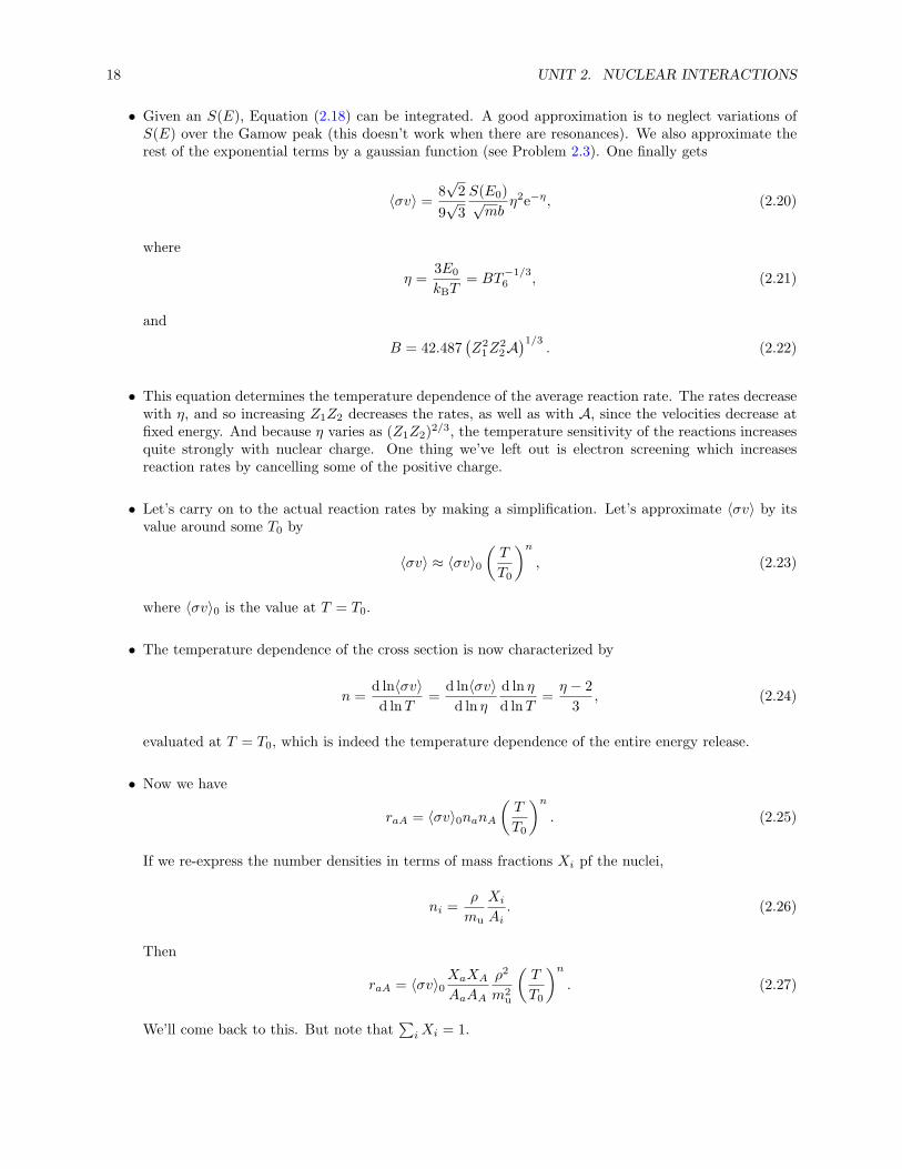
• Given an S(E), Equation (2.18) can be integrated. A good approximation is to neglect variations ofS(E) over the Gamow peak (this doesn’t work when there are resonances). We also approximate therest of the exponential terms by a gaussian function (see Problem 2.3). One finally gets
〈σv〉 = 8√2
9√3
S(E0)√mb
η2e−η, (2.20)
where
η =3E0
kBT= BT
−1/36 , (2.21)
and
B = 42.487(
Z21Z
22A)1/3
. (2.22)
• This equation determines the temperature dependence of the average reaction rate. The rates decreasewith η, and so increasing Z1Z2 decreases the rates, as well as with A, since the velocities decrease atfixed energy. And because η varies as (Z1Z2)
2/3, the temperature sensitivity of the reactions increasesquite strongly with nuclear charge. One thing we’ve left out is electron screening which increasesreaction rates by cancelling some of the positive charge.
• Let’s carry on to the actual reaction rates by making a simplification. Let’s approximate 〈σv〉 by itsvalue around some T0 by
〈σv〉 ≈ 〈σv〉0(
T
T0
)n
, (2.23)
where 〈σv〉0 is the value at T = T0.
• The temperature dependence of the cross section is now characterized by
n =d ln〈σv〉d lnT
=d ln〈σv〉d ln η
d ln η
d lnT=
η − 2
3, (2.24)
evaluated at T = T0, which is indeed the temperature dependence of the entire energy release.
• Now we have
raA = 〈σv〉0nanA
(
T
T0
)n
. (2.25)
If we re-express the number densities in terms of mass fractions Xi pf the nuclei,
ni =ρ
mu
Xi
Ai. (2.26)
Then
raA = 〈σv〉0XaXA
AaAA
ρ2
m2u
(
T
T0
)n
. (2.27)
We’ll come back to this. But note that∑
i Xi = 1.
2.4. PROBLEMS 19
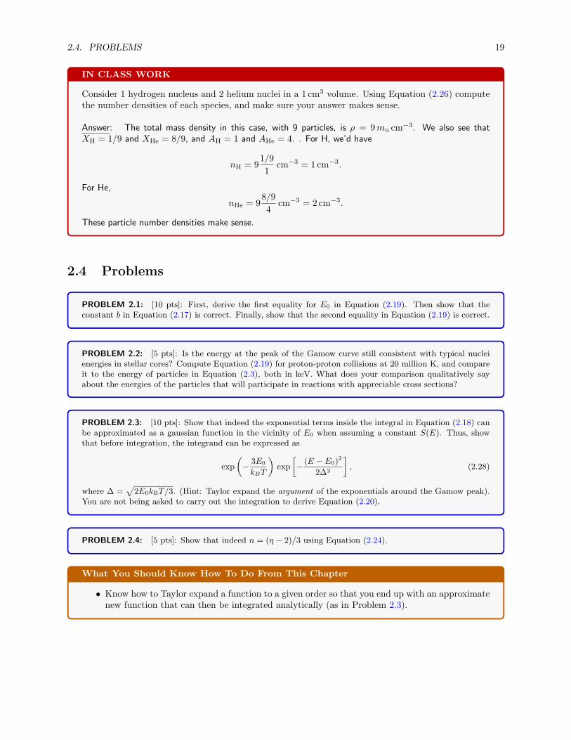
IN CLASS WORK
Consider 1 hydrogen nucleus and 2 helium nuclei in a 1 cm3 volume. Using Equation (2.26) computethe number densities of each species, and make sure your answer makes sense.
Answer: The total mass density in this case, with 9 particles, is ρ = 9mu cm−3. We also see that
XH = 1/9 and XHe = 8/9, and AH = 1 and AHe = 4. . For H, we’d have
nH = 91/9
1cm−3 = 1 cm−3.
For He,
nHe = 98/9
4cm−3 = 2 cm−3.
These particle number densities make sense.
2.4 Problems
PROBLEM 2.1: [10 pts]: First, derive the first equality for E0 in Equation (2.19). Then show that theconstant b in Equation (2.17) is correct. Finally, show that the second equality in Equation (2.19) is correct.
PROBLEM 2.2: [5 pts]: Is the energy at the peak of the Gamow curve still consistent with typical nucleienergies in stellar cores? Compute Equation (2.19) for proton-proton collisions at 20 million K, and compareit to the energy of particles in Equation (2.3), both in keV. What does your comparison qualitatively sayabout the energies of the particles that will participate in reactions with appreciable cross sections?
PROBLEM 2.3: [10 pts]: Show that indeed the exponential terms inside the integral in Equation (2.18) canbe approximated as a gaussian function in the vicinity of E0 when assuming a constant S(E). Thus, showthat before integration, the integrand can be expressed as
exp
(
−3E0
kBT
)
exp
[
−(E − E0)
2
2∆2
]
, (2.28)
where ∆ =√
2E0kBT/3. (Hint: Taylor expand the argument of the exponentials around the Gamow peak).You are not being asked to carry out the integration to derive Equation (2.20).
PROBLEM 2.4: [5 pts]: Show that indeed n = (η − 2)/3 using Equation (2.24).
What You Should Know How To Do From This Chapter
• Know how to Taylor expand a function to a given order so that you end up with an approximatenew function that can then be integrated analytically (as in Problem 2.3).

20 UNIT 2. NUCLEAR INTERACTIONS
Unit 3
Energy release in nuclear reactions
3.1 Mass excess
• Just recall some definitions (ignoring electrons):
– Atomic number Z: number of protons in a nucleus. ZH = 1, ZHe = 2, etc. Always an integer.
– Mass number A: number of protons Z and neutrons N in a nucleus. Always an integer.
– Atomic mass: The true mass of a single atom (single isotope). A number very nearly equal to themass number A when expressed in amu. Can be greater or less than A.
– Atomic weight: The averaged mass over all isotopes of an element (typically what is given in aperiodic table). Usually greater than A.
– Atomic mass unit, amu: 1/12 the mass of neutral carbon 12.
• Consider the reaction of nucleia+A −→ y + Y. (3.1)
Conservation of energy requires
Ea,A + (ma +mA)c2 = Ey,Y + (my +mY )c
2, (3.2)
where the Ei,I on each side is the kinetic energy of the center-of-mass of each system. Also includedare the rest mass energies of each species.
• We can rewrite Equation (3.2) asEy,Y = Ea,A +Q, (3.3)
whereQ = c2[ma +mA −my −mY ]. (3.4)
The quantity Q can be interpreted as the energy released in any reaction, or, the increase in energyfor each reaction.
• Note that these reactions are taking place among nuclei. However, since charge is conserved, wemay replace the nuclear masses implied in the above equations with the atomic masses, because thesame number of electron rest masses will be added to both sides of the equation. A small error inthe neglected electron binding energy is introduced (of a few eV), but the great convenience in usingatomic masses is well worth it.
• Also conserved in these reactions is the number of nucleons, and it is convenient to remove theircontribution as it will not change the energy budget. The way to do this is to consider that the massnumber is the nearest integer to the exact mass of an atom in atomic mass units.
21

22 UNIT 3. ENERGY RELEASE IN NUCLEAR REACTIONS
• So consider an atom with Z protons, N neutrons, and A = Z +N nucleons, with atomic mass m. Wecan derive what’s known as the mass excess or mass defect ∆m (which has units of energy):
∆m = (m− (Z +N)mu)c2,
= (m−Amu)c2
= [m(amu)−A] c2mu,
or finally,∆m = 931.494MeV [m(amu)−A] [MeV], (3.5)
where m(amu) is the atomic mass of the nucleon in question in amu, and 1mu = 931.5MeV/c2.
• Note, mass excess is really just the difference between the atomic mass of an element (which is usuallya number with a very small decimal addition) and its mass number (which is always an integer, A).
• Mass excesses are given in the table in Figure 3.6. As an example of using the above expression tocome up with these values, take 4He. Its atomic mass m = 4.002602. It has 4 nucleons. So
∆m = (931.494)(4.002602− 4) = 2.44MeV. (3.6)
(slightly different than the table because of updated atomic masses).
• We can therefore write for the energy release of some reaction in terms of mass excesses:
QaA = [∆m(a) + ∆m(A)−∆m(y)−∆m(Y )]. (3.7)
• In general, the energy is released as kinetic energy to the resultant particles (as implied in Equa-tion (3.3)), and sometimes in photons (and neutrinos, which isn’t too important in the energy budgetfor normal reactions). The energy gets redistributed in the gas through collisions and the absorptionof photons. The details don’t matter because of energy equilibrium, but what matters is the totalamount of heat added to the gas.
• Back to Equation (2.27), the energy generation rate per gram is the reaction rate multiplied by theenergy for each reaction divided by density, so
εaA =raAQaA
ρ, [erg g−1 s−1], (3.8)
εaA = QaA〈σv〉0XaXA
AaAA
ρ
m2u
(
T
T0
)n
. (3.9)
• One can in general writeε = ε0ρT
n, (3.10)
for any reaction, absorbing most of the constant terms in ε0.
3.2 Binding energy
• Do not confuse mass excess with nuclear binding energy, since they are very similar.
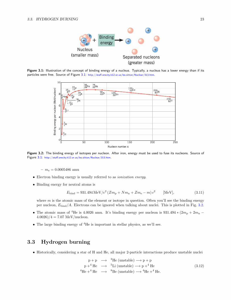
• The nuclear binding energy is the energy required to separate a stable nucleus into its constituentparts, as depicted in Figure 3.1. Note the following definitions:
– 1 amu = 931.494MeV/c2 = mu
– mp = 1.007825 amu
– mn = 1.00867 amu
3.3. HYDROGEN BURNING 23
Figure 3.1: Illustration of the concept of binding energy of a nucleus. Typically, a nucleus has a lower energy than if itsparticles were free. Source of Figure 3.1: http://staff.orecity.k12.or.us/les.sitton/Nuclear/313.htm.
Figure 3.2: The binding energy of isotopes per nucleon. After iron, energy must be used to fuse its nucleons. Source ofFigure 3.1: http://staff.orecity.k12.or.us/les.sitton/Nuclear/313.htm.
– me = 0.0005486 amu
• Electron binding energy is usually referred to as ionization energy.
• Binding energy for neutral atoms is
Ebind = 931.494MeV/c2 (Zmp +Nmn + Zme −m) c2 [MeV], (3.11)
where m is the atomic mass of the element or isotope in question. Often you’ll see the binding energyper nucleon, Ebind/A. Electrons can be ignored when talking about nuclei. This is plotted in Fig. 3.2.
• The atomic mass of 4He is 4.0026 amu. It’s binding energy per nucleon is 931.494 ∗ (2mp + 2mn −4.0026)/4 = 7.07 MeV/nucleon.
• The large binding energy of 4He is important in stellar physics, as we’ll see.
3.3 Hydrogen burning
• Historically, considering a star of H and He, all major 2-particle interactions produce unstable nuclei
p + p −→ 2He (unstable) −→ p + p
p +4 He −→ 5Li (unstable) −→ p +4 He (3.12)4He +4 He −→ 8Be (unstable) −→ 4He +4 He.

24 UNIT 3. ENERGY RELEASE IN NUCLEAR REACTIONS
• It was Hans Bethe who first showed that the weak force plays a role in all this, in the form of betadecay (see below).
• Anyway, the general idea of hydrogen fusion is always
41H −→4He + 2e+ + 2νe, (3.13)
where 2 positrons are needed to keep charge conserved, and 2 electron neutrinos conserve lepton number(from the 2 anti-lepton positrons). This does not happen all at once, but along certain “paths,” seebelow.
• The atomic mass of H is 1.007852 amu and of 4He is 4.002603 amu. So 0.0288 mass units are lost. Themass fraction that is turned into energy is thus 0.0288/4 = 0.007, or 0.7%.
• Using ∆mc2, we have (0.0288)(931.494MeV/c2)c2 = 26.8MeV.
• Using the mass excesses in the units of MeV we can compute the energy liberated in yet another way
Q = 4(7.289)− 2.4248− 2(0.263) = 26.21MeV, (3.14)
where this time we take into account the energy carried away by the neutrinos (see table in Fig. 3.3).Note, as mentioned before, that the values are from atomic mass excesses, not nuclear mass excesses, soelectrons are implicitly in there (including . That is why we do not take into account the∼ 0.5 MeV fromthe positrons (since those, plus the 2 electrons on the RHS implicit in the the He, cancel energeticallywith the 4 electrons implicit on the LHS).
• Let’s be redundant, and clear. Consider the energy available to the star (sometimes referred to as theeffective energy) for a generic β decay process, whereby a proton converts to a neutron in some nucleus,producing a positron and neutrino as well. This energy can be written as (using our notation)
Q = ∆mnuc(Z + 1)−∆mnuc(Z)−mec2 + 2mec
2 − Eν ,
= ∆mnuc(Z + 1)−∆mnuc(Z) +mec2 − Eν ,
= ∆matom(Z + 1)−∆matom(Z)− Eν ,
where the ∆m are the mass excesses (in energy units), Z is the proton number of the nucleus, Eν is theenergy carried off by the neutrino (not available to the star), the −mec
2 is the energy required to createthe positron, and the +2mec
2 is the energy produced when the electron-positron annihiliation takesplace (gamma radiation is typically produced). At one point we switched from using “nuclear” massexcesses to “atomic” ones (as the ones in the tables) which take into account electron contributions.That’s why the electrons are “already counted” in the energy budget, at some level.
3.3.1 PP-I chain
• The proton-proton reaction is
1H+1 H −→ 2D+ e+ + ν = 2(7.289)− 13.136− 0.263 = 1.18MeV; (109 yr)2D+1 H −→ 3He + γ = 13.136 + 7.289− 14.93 = 5.49MeV; (6 s),
3He +3He −→ 4He +1 H+1 H = 2(14.93)− 2.42− 2(7.289) = 12.86MeV; (106 yr)
Noting that the first two reactions have to happen twice to produce 2 3He nuclei, the total energy is2(1.18)+2(5.49)+12.86 = 26.2 MeV, as we saw before.
• Another way to write this is
1H(1H, e+νe)2D(1H, γ)3He(3He, 21H)4He, (3.15)
where everything to the left of the comma is an ingredient of the reaction, and everything to the rightis a product.
3.3. HYDROGEN BURNING 25
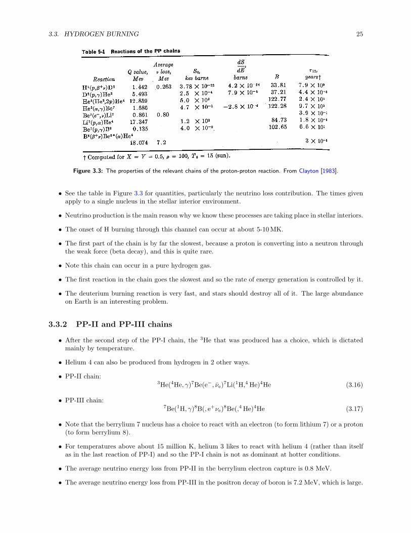
Figure 3.3: The properties of the relevant chains of the proton-proton reaction. From Clayton [1983].
• See the table in Figure 3.3 for quantities, particularly the neutrino loss contribution. The times givenapply to a single nucleus in the stellar interior environment.
• Neutrino production is the main reason why we know these processes are taking place in stellar interiors.
• The onset of H burning through this channel can occur at about 5-10MK.
• The first part of the chain is by far the slowest, because a proton is converting into a neutron throughthe weak force (beta decay), and this is quite rare.
• Note this chain can occur in a pure hydrogen gas.
• The first reaction in the chain goes the slowest and so the rate of energy generation is controlled by it.
• The deuterium burning reaction is very fast, and stars should destroy all of it. The large abundanceon Earth is an interesting problem.
3.3.2 PP-II and PP-III chains
• After the second step of the PP-I chain, the 3He that was produced has a choice, which is dictatedmainly by temperature.
• Helium 4 can also be produced from hydrogen in 2 other ways.
• PP-II chain:3He(4He, γ)7Be(e−, νe)
7Li(1H,4 He)4He (3.16)
• PP-III chain:7Be(1H, γ)8B(, e+νe)
8Be(,4 He)4He (3.17)
• Note that the berrylium 7 nucleus has a choice to react with an electron (to form lithium 7) or a proton(to form berrylium 8).
• For temperatures above about 15 million K, helium 3 likes to react with helium 4 (rather than itselfas in the last reaction of PP-I) and so the PP-I chain is not as dominant at hotter conditions.
• The average neutrino energy loss from PP-II in the berrylium electron capture is 0.8 MeV.
• The average neutrino energy loss from PP-III in the positron decay of boron is 7.2 MeV, which is large.
26 UNIT 3. ENERGY RELEASE IN NUCLEAR REACTIONS
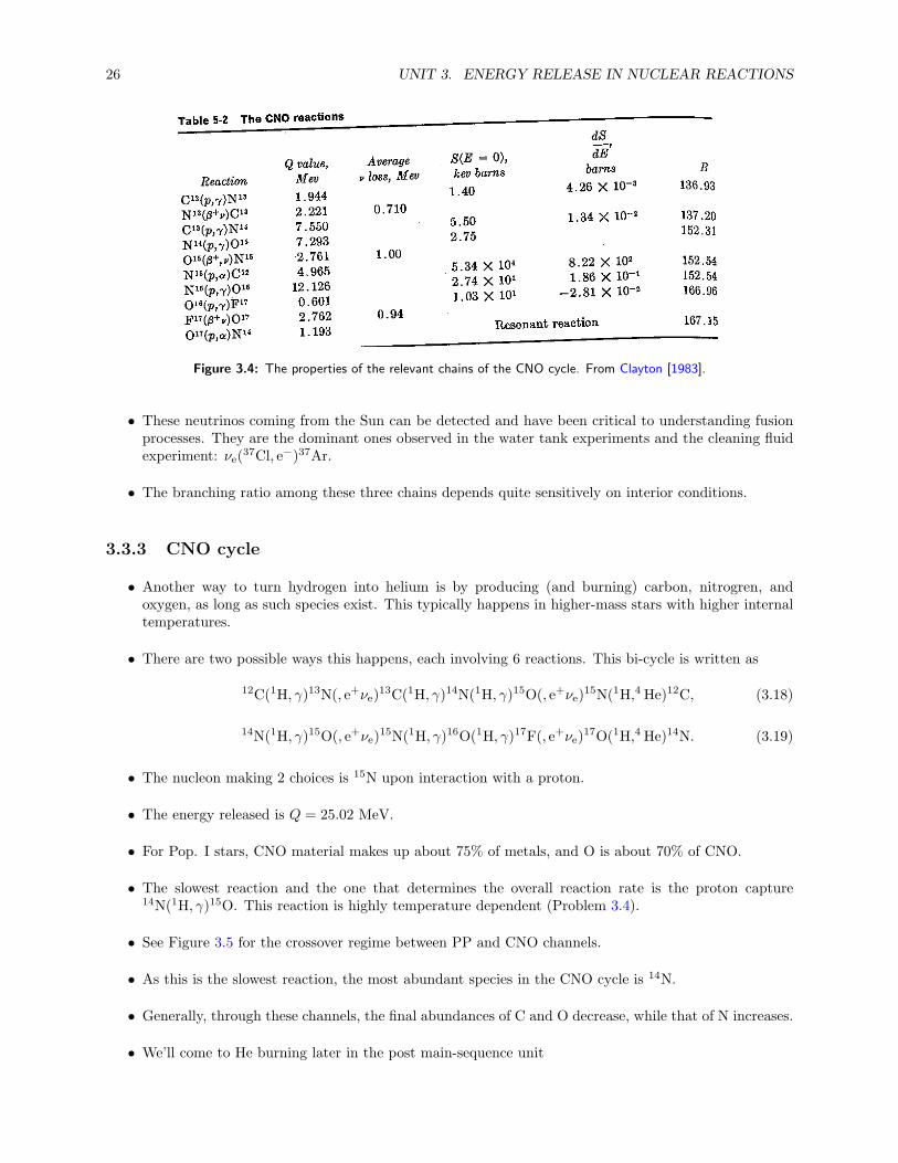
Figure 3.4: The properties of the relevant chains of the CNO cycle. From Clayton [1983].
• These neutrinos coming from the Sun can be detected and have been critical to understanding fusionprocesses. They are the dominant ones observed in the water tank experiments and the cleaning fluidexperiment: νe(
37Cl, e−)37Ar.
• The branching ratio among these three chains depends quite sensitively on interior conditions.
3.3.3 CNO cycle
• Another way to turn hydrogen into helium is by producing (and burning) carbon, nitrogren, andoxygen, as long as such species exist. This typically happens in higher-mass stars with higher internaltemperatures.
• There are two possible ways this happens, each involving 6 reactions. This bi-cycle is written as
12C(1H, γ)13N(, e+νe)13C(1H, γ)14N(1H, γ)15O(, e+νe)
15N(1H,4 He)12C, (3.18)
14N(1H, γ)15O(, e+νe)15N(1H, γ)16O(1H, γ)17F(, e+νe)
17O(1H,4 He)14N. (3.19)
• The nucleon making 2 choices is 15N upon interaction with a proton.
• The energy released is Q = 25.02 MeV.
• For Pop. I stars, CNO material makes up about 75% of metals, and O is about 70% of CNO.
• The slowest reaction and the one that determines the overall reaction rate is the proton capture14N(1H, γ)15O. This reaction is highly temperature dependent (Problem 3.4).
• See Figure 3.5 for the crossover regime between PP and CNO channels.
• As this is the slowest reaction, the most abundant species in the CNO cycle is 14N.
• Generally, through these channels, the final abundances of C and O decrease, while that of N increases.
• We’ll come to He burning later in the post main-sequence unit

3.4. PROBLEMS 27
Figure 3.5: The nuclear energy rate as a function of temperature. The Sun is marked as a circle. From Salaris and Cassisi[2006].
3.4 Problems
PROBLEM 3.1: [5 pts]: The Sun’s luminosity is L⊙ = 3.9 × 1033 erg s−1. Assume that the energy for thisluminosity is provided solely by the PP-I chain, and that neutrinos carry off 3% of the energy liberated. Howmany neutrinos are produced per second? What is the neutrino flux at Earth (# neutrinos per second percm2)?
PROBLEM 3.2: [5 pts]: Show that at a temperature of T = 15 MK the temperature exponent (Equa-tion (2.24)) in the first reaction of the PP-I chain is n ≃ 4.
PROBLEM 3.3: [10 pts]: Compute the full Q values for the PP-II and PP-III chains (don’t forget to includeany necessary contributions from previous chains in the computation).
PROBLEM 3.4: [5 pts]: Show that at a temperature of T = 15 MK the temperature exponent in the slowestreaction of the CNO cycle is n ≃ 20.
What You Should Know How To Do From This Chapter
• Understand how to compute the temperature dependence of nuclear reactions (given the specificformula)

28 UNIT 3. ENERGY RELEASE IN NUCLEAR REACTIONS
Figure 3.6: Mass excesses from Clayton [1983].
Unit 4
Distribution functions
In Unit 6 we will start to derive equations of state of stellar matter. To do so from first principles, we needto know how, in general, particles are distributed as a function of momentum (or energy). This requiressome basic statistical mechanics.
Statistical mechanics deals with the occupation of energy states when a system is excited. The fundamentalassumption of statistical mechanics is that, in thermal equilibium, every distinct state with the same totalenergy is occupied with equal probability. Temperature is simply a measure of the total energy of a systemin thermal equilibium. The only change from classical statistical mechanics to quantum mechanics has todo with how we count distinct states, which depends on whether the particles involved are distinguishable,identical fermions, or identical bosons.
4.1 An example
• Consider 3 non-interacting particles of equal mass in some potential.
• The total energy of the system is 243 (with some arbitrary energy units). This means that the particlesoccupy some energy levels ni such that, using a simple and arbitrary energy rule, we have
Etotal =∞∑
i=1
nii2 = 243. (4.1)
A one-dimensional square well, for example, has a dispersion relation like this one. There would beprefactors before the summation symbol to give the right units of energy; for simplicity, ignore suchterms.
• Consider distinguishable (classical) particles. There are 13 unique ways of distributing 3 particles intovarious energy levels to get a total energy of 243.
– We can have all 3 particles in the 9th state: n9 = 3. There is only 1 way of doing this.
– n1 = 1, n11 = 2. (3 ways)
– n3 = 2, n15 = 1. (3 ways)
– n5 = n7 = n13 = 1. (6 ways)
• Quantum statistics says, for large N, that all states with the same N and same Etotal are equally likely.
• Therefore, in thermal equilibrium, the most probable configuration is the one that can be achieved inthe largest number of ways. The last state is this case. We’ll come back to this.
• Now consider fermions, which are indistinguishable, and cannot occupy the same state.
29

30 UNIT 4. DISTRIBUTION FUNCTIONS
• There is only one possibility here: n5 = n7 = n13 = 1.
• Finally, consider bosons, which are indistinguishable. There are 3 distinct states:
– n9 = 3. (1 way)
– n3 = 2, n15 = 1. (1 way)
– n5 = n7 = n13 = 1. (1 way)
4.2 Partition function
• Again consider N particles with the same masses. There are energy states Ei with degeneracies gi(distinct states with same energy Ei). We distribute the N particles such that there are N1 particleswith energy E1, N2 particles with energy E2, etc. We want to know how many different ways we cando this?
• We now define Q(n1, n2, n3, . . .) to be the number of microscopically distinguishable arrangements thatlead to the same macroscopic distribution.
• It is sometimes known as a partition function, or probability distribution function, or canonical en-semble, etc.
• Clearly, Q depends strongly on the type of particle we are considering, as the 3 cases below show(without derivation).
4.2.1 Distinguishable particles
In this case,
Q = N !∞∏
i=1
gnii
ni!
To prove this, we go back to the previous illustration:
Q(n9 = 3) = 3!
(
13
3!
)
= 1. (4.2)
Q(n3 = 2, n15 = 1) = 3!
(
12
2!
)(
11
1!
)
= 3. (4.3)
Q(n5 = 1, n7 = 1, n13 = 1) = 3!
(
11
1!
)(
11
1!
)(
11
1!
)
= 6. (4.4)
This confirms our earlier counting.
4.2.2 Identical fermions
In this case,
Q =
∞∏
i=1
gi!
ni! (gi − ni)!.
So,
Q(n5 = 1, n7 = 1, n13 = 1) =
(
1!
1!0!
)(
1!
1!0!
)(
1!
1!0!
)
= 1. (4.5)
4.3. DERIVATION 31
4.2.3 Identical bosons
In this case,
Q =
∞∏
i=1
(ni + gi − 1)!
ni!(gi − 1)!.
4.3 Derivation
In thermal equilibirum, each energy state with some occupying number of particles is equally likely. Themost probable configuration is one that can be obtained with the largest number of different ways, such thatQ(ni) is maximum. The only constraints in this problem are that the total number of particles in eachstate add up to the total, or
∑
i
ni = N,
and that the total energy is maintained as
∑
i
niEi = Etot.
To solve such a problem we can introduce a new function and Lagrange multipliers that help maintain theconstraints. Instead of maximizing Q, it’s more convenient to consider lnQ. So we want to maximize
G = lnQ+ α
[
N −∑
i
ni
]
+ β
[
Etot −∑
i
niEi
]
.
Then to find the maximum we compute ∂G/∂nj = 0. Also, regarding the Lagrange multipliers, ∂G/∂α = 0and ∂G/∂β = 0 simply reproduce the constraints.
The quantity Q needs to be considered for the 3 different types of particles that we’ve discussed.
It will also be helpful to utilize Stirling’s approximation:
ln(x!) ≈ x lnx− x, (4.6)
which holds when x≫ 1.
1. Distinguishable particles. Do this in detail. Using our Q in this case we have
G = lnN ! + ln∏
i=1
gnii
ni!+ α
[
N −∑
i
ni
]
+ β
[
E −∑
i
niEi
]
= lnN ! +∑
i
lngnii
ni!+ α
[
N −∑
i
ni
]
+ β
[
E −∑
i
niEi
]
= lnN ! +∑
i
ni ln gi −∑
i
lnn! + α
[
N −∑
i
ni
]
+ β
[
E −∑
i
niEi
]
= N lnN −N +∑
i
ni ln gi −∑
i
ni lnni +∑
i
ni + α
[
N −∑
i
ni
]
+ β
[
E −∑
i
niEi
]
.
Note E ≡ Etot.
32 UNIT 4. DISTRIBUTION FUNCTIONS
Now taking the partial derivative
∂G
∂nj= ln gj − lnnj −
nj
nj+ 1− α− βEj = 0
= ln gj − lnnj − α− βEj = 0
lngjnj
= α+ βEj
gjnj
= eα+βEj
nj = gje−α−βEj .
This is the result we are looking for.
2. Fermions. Following the same procedure, we find
nj =gj
exp(α+ βEj) + 1.
3. Bosons. Again, the same procedure yields
nj =gj
exp(α+ βEj)− 1.
To determine what α and β are, one needs to plug the nj into the constraints and consider some specifictotal particle number N and energy system E. One then finds that
α = − µ
kBT,
β =1
kBT,
where µ is the chemical potential and kB is Boltzmann’s constant.
Unit 5
Mean molecular weight
• Another concept before we dive into equations of state is the mean molecular weight µ, which isimportant to understand.
• Stellar interiors have a mixture of atoms of different elements and various ionizations.
• Consider the mean mass m per particle
m =
∑
j nj,Imj,I + neme∑
j nj,I + ne≈∑
j nj,Imj,I∑
j nj,I + ne, (5.1)
where nj,I is the ion number density of ion j, mj,I is its mass, and ne and me are the numbers andmass of the electron (and then we ignore the electron mass).
• The mass of the jth ion is approximately its number of protons and neutrons (Aj) times the amu, ormj,I = Ajmu.
• So then we define
µ =m
mu=
∑
j nj,IAj∑
j nj,I + ne. (5.2)
This can be interpreted as the average mass per particle (ion, electron, etc.) in units of the amu.
• Note that the total particle number density in the gas is
n = ne + nI = ne +∑
j
nj,I =∑
j
(1 + Zj)nj,I, (5.3)
since one ionized atom contributes 1 nucleus plus Zj electrons. The total ne =∑
j nj,IZj , where Zj isthe “charge” of each nucleus.
• In general though, the electron density (or level of ionization) is complicated and derived from theSaha equation. Such an equation gives ionization fractions yi such that the electron number densitywould be ne =
∑
j nj,IyjZj (see later).
• But to be more useful, it’s easier to express the number densities in terms of mass fractions xi, where∑
i xi = 1.
• The number densities we looked at earlier are for some species i are
ni =ρ
mu
xi
Ai. (5.4)
Think of this as the mass per unit volume of species i (ρxi), in units of 1 ion of species i (muAi).
33
34 UNIT 5. MEAN MOLECULAR WEIGHT
IN CLASS WORK
Imagine a star where 92% of all particles are hydrogen nuclei and 8% of them are helium nuclei.What are the mass fractions of hydrogen and helium?
92 =ρxH
mu
8 =ρxHe
4mu
xH = 92mu/ρ
xHe = 32mu/ρ
92mu/ρ+ 32mu/ρ = 124mu/ρ = 1
mu/ρ = 1/124
xH = 92/124 = 0.7419
xHe = 32/124 = 0.2581.
• So using this, we now have
µ =
∑
iρ
muxi
∑
iρxi
muAi+ ne
, (5.5)
or
µ =
∑
iρ
muxi
∑
iρxi
muAi(1 + Zi)
. (5.6)
• One cleaner way of writing this is
µ−1 =
∑
i xi/Ai(1 + Zi)∑
i xi=∑
i
xi
Ai(1 + Zi). (5.7)
• For example, for a neutral gas (Z = 0) we have
µ−1 =∑
i
xi
Ai≈(
X +Y
4+
Z
Ai
)−1
, (5.8)
where it is standard to write mass fractions X for hydrogen, Y for helium, and Z for everything else(metals), where X + Y + Z = 1.
• Ai is an average over metals, which at solar composition is about 15.5.
• For a fully ionized gas
µ−1 ≈∑
i
xi
Ai(1 + Zi) ≈ 2X +
3
4Y +
1
2Z, (5.9)
or
µ ≈ 4
3 + 5X − Z, (5.10)
where for metals we usually approximate (1 + Zi)/Ai ≈ 1/2 (roughly equal number of protons andneutrons). We’ve eliminated Y in this expression through Y = 1−X − Z.
35
IN CLASS WORK
Compute the mean molecular weight for (1) the ionized solar photosphere, where we have 90%hydrogen, 9% helium, and 1% heavy elements by mass, (2) the ionized solar interior where 71%hydrogen, 27% helium, and 2% heavy elements by mass, (3) completely ionized hydrogen, (4)completely ionized helium, and finally (5) neutral gas at the solar interior abundance.
Answer: (1) For the photosphere we can write
µ−1 = 0.92
1+ 0.09
3
4+ 0.01
1
2= 1.8725,
or µ ≈ 0.53.(2) For the interior we can write
µ−1 = 0.712
1+ 0.27
3
4+ 0.02
1
2= 1.63,
or µ ≈ 0.61.(3) For hydrogen, we will take X = Z = A = 1, and find then that 1/µ = 2.(4) For helium, X = Z = 0 and Y = 1, so µ = 4/3.(5) For a neutral gas, we have
µ−1 = 0.71 + 0.271
4+ 0.02
1
15.5= 0.779,
or µ ≈ 1.28.
• From the above, we can also consider separately the mean molecular weight for ions and electrons.
• For ions, define µI as
nI =ρ
µImu. (5.11)
Recall that
nI =∑
j
nj,I =ρ
mu
∑
j
xj
Aj. (5.12)
So that
µI =
∑
j
xj
Aj
−1
. (5.13)
• This result should make sense, since above in Equation (5.8) we did not consider electrons.
• For electrons it’s a bit harder since not all electrons need be free. But we will still define the mean
molecular weight per election µe:
ne =ρ
µemu(5.14)
• Fully ionized, each atom contributes Z electrons. If an ion is partially ionized, we can consider thefraction yZ. (To compute the proper fraction of ionization of a gas (ne), one needs to use the Saha
equation).
• As before then
ne =∑
j
ne,j =∑
j
nj,IyjZj =ρ
mu
∑
j
(
xj
Aj
)
yjZj , (5.15)
36 UNIT 5. MEAN MOLECULAR WEIGHT
which defines
µe =
∑
j
xjyjZj
Aj
−1
. (5.16)
• So finally
n = ne + nI =ρ
µmu, (5.17)
where
µ =
(
1
µI+
1
µe
)−1
. (5.18)
IN CLASS WORK
Compute an expression for µe in the deep stellar interior as a function only of X. Ignore metals.
Answer: Fully ionized case. We can write
µe ≈(
1
1X +
2
4Y
)−1
=
(
X +1
2(1−X)
)−1
=
(
X + 1
2
)−1
=2
1 +X.
This should make sense. For a full H gas, the mean mass of particles per number of electrons (1/1) is 1.For a He gas (X = 0), we have a mass of 4 divided by 2 electrons, or µe = 2.

Unit 6
Equation of state: Ideal gas
6.1 Preliminaries
• First we recall the distribution function and do a little thermodynamics with them.
• A distribution function simply measures the number density of a species in 6D space of position andmomentum.
• If we know this function for a gas, all thermodynamic quantities can be derived (pressure, temperature,density, composition).
• Equations of state relate pressure, temperature, and number of particles.
• An ideal gas is one in which the particles don’t interact (except through elastic collisions). They canexchange energy though, but have to conserve it.
• This approximation breaks down when matter is degenerate, and particles begin to “sense” each otherand interact in quantum fashion or otherwise.
• An important thermodynamical quantity is the chemical potential µc for each species, that was in-troduced earlier. For classical particles, µc → −∞, for degenerate fermions µc → ǫF, for bosonsµc = 0.
• Chemical changes in the gas use the chemical potential to monitor particle numbers, and thus toachieve a chemical equilibrium (in addition to thermodynamic equilibrium).
• In thermodynamic equilibrium, statistical mechanics tells us the relationship between the numberdensity (of phase space, ie, number per unit volume per unit momentum: d3r d3p) of a species
n(p) =1
h3
∑
j
gjexp {[Ej + E(p)− µc] /kBT} ± 1
, (6.1)
where
– j are the possible energy states of the species (like energy levels in an ion), and Ej is the energyof that level
– E(p) is the kinetic energy
– gj is the degeneracy of state j (number of states with same energy)
– ± is either for fermions or bosons, respectively.
Note that the units of Planck’s constant are length times momentum (remember the uncertaintyprinciple). We will come back to this frequently.
37

38 UNIT 6. EQUATION OF STATE: IDEAL GAS
• To find the number density (particles cm−3) we integrate n(p) d3p over momentum space (assumed tobe symmetric)
n =
∫
p
4πp2n(p) dp. (6.2)
• To remain completely general, the kinetic energy of a particle of rest mass m is
E(p) = (p2c2 +m2c4)1/2 −mc2. (6.3)
IN CLASS WORK
What does this expression reduce to in the nonrelativistic limit?
Answer: In this limit, we note that pc≪ mc2, so one can expand the term in the square root:
E(p) = mc2(
1 +p2c2
m2c4
)1/2
−mc2,
≈ mc2(
1 +1
2
p2c2
m2c4
)
−mc2,
≈ p2
2m,
which is the expression we’d expect.
• Now we can define three general quantities:
1. Velocity:
v =∂E
∂p. (6.4)
2. Pressure:
P =
∫
pn(p)v · p d3p =
1
3
∫
p
n(p)v p 4πp2 dp, (6.5)
where the last equality comes from assuming isotropy of pressure.
3. Internal energy density (energy per unit volume):
u =
∫
p
n(p)E(p)4πp2 dp. (6.6)
• These general considerations can soon be applied to specific cases.
6.2 Maxwell-Boltzmann statistics
• The relation of Equation (6.1) to classical probability functions is found through Equation (6.11) andEquation (6.12). These tell us the fraction of particles within an infinitesimal element of 3-dimensionalspace (velocity, energy, or momentum space).
• In momentum space
f(p) dp =4π
(2πmkBT )3/2e−p2/2mkT p2 dp. (6.7)
• In energy space
f(E) dE =2√
π(kBT )3/2e−E/kT
√E dE. (6.8)

6.3. IDEAL MONATOMIC GAS 39
• In velocity space
f(v) dv = 4π
(
m
2πkBT
)3/2
e−mv2/2kT v2 dv. (6.9)
• These are normalized such that the integrals of each quantity over velocity, momentum, or energy areequal to 1.
6.3 Ideal monatomic gas
• As a first demonstration, we consider a gas of single species nonrelativistic particles. We will be usingEquation (6.1).
• Their energy is E = p2/2m. Consider one energy level Ej = E0.
• For this system, the chemical potential goes to negative infinity (as we’ll see), so the exponential termis large, and the ±1 term can be safely ignored.
• The number density of particles in any given momentum state p is
n(p) =g
h3e−p2/2mkT e−E0/kT eµc/kT , (6.10)
and so the total number density over all momenta is
n =4πg
h3
∫ ∞
0
p2e−p2/2mkT e−E0/kT eµc/kT dp. (6.11)
• The integral is straightforward and gives an expression
n =(2πmkBT )
3/2g
h3e−E0/kT eµc/kT . (6.12)
• Another way to write this is
eµc/kT =nh3
g(2πmkBT )3/2eE0/kT . (6.13)
Since we are assuming that the term on the left is small (since µc ≪ −1), then the right hand sidemust also be small. Specifically, nT−3/2 cannot be too large. If that were the case, then we would notbe able to ignore the ±1 term in the distribution function.
• Returning to the definition of gas pressure in Equation (6.5), we can compute the integral to find
P = g4π
h3
π1/2
8m(2mkBT )
5/2e−E0/kT eµc/kT . (6.14)
• Using the generalized number density from Equation (6.12), this gives what you thought it would
P = nkBT [dyne cm−2]. (6.15)
This is the equation of state for an ideal gas.
• Similarly we can compute the internal energy density from Equation (13.6)
u =3
2nkBT =
3
2P ; [erg cm−3]. (6.16)
• Note that the units of pressure and internal energy density are the same.
40 UNIT 6. EQUATION OF STATE: IDEAL GAS
• From what we saw before with the mean molecular weight, we can also express these quantities as
n =ρ
µmu, (6.17)
P =ρkBT
µmu, (6.18)
P =ρRT
µ, (6.19)
where µ is the mean molecular weight, and R = kB/mu is the ideal gas constant R = 8.31 ×10⁷ ergK−1 mol−1.
EXAMPLE PROBLEM 6.1: Instead of arriving at Equation (6.16) through the energy formulation, one canuse velocity to show that the average internal kinetic energy per particle is 3/2kBT . Hint: Start with theMaxwellian distribution for a classical gas in velocity (Equation (6.9)) and then compute the mean squarespeed 〈v2〉. The integration limits of v should be from zero to infinity.
Answer: The mean square speed can be written as
〈v2〉 =
∫
∞
0
v2f(v)dv,
where f(v) is the Maxwell distribution. One can (and should) use a table of integrals to find that
∫
∞
0
xne−ax2
dx =(2k − 1)!!
2k+1ak
(π
a
)1/2
,
where n = 2k and in our case a = m/2kBT > 0. Note the double factorial, which, for k = 2, is 3× 1 = 3. Theresult is
〈v2〉 = 4π
(
m
2πkBT
)3/2
·3
8
π1/2
a5/2,
and after cancellation becomes
〈v2〉 =3kBT
m.
The kinetic energy is then 1/2m〈v2〉 = 3/2kBT , precisely what we set out to prove.
Unit 7
Equation of state: Degenerate gas
7.1 Completely degenerate gas
• The ideal gas law (because of Maxwell-Boltzmann statistics) breaks down at sufficiently high densitiesand/or low temperatures.
• Consider the extreme case where T → 0 at fixed density.
• From Equation (6.7), the Maxwell distribution peaks at zero momentum where all the particles wantto pile up. They want to be in the lowest energy state, which is zero.
• There’s a limit to how close fermions can come, based on the Pauli exclusion principle.
• So instead, we must use Fermi-Dirac statistics and not Maxwell-Boltzmann.
• Consider first the most interesting terms in Equation (6.1)
f(p) =1
e(E(p)−µc)/kT + 1, (7.1)
where we’ve taken a reference energy level Ej = 0.
• As T → 0, f goes to 1 or 0 depending on the sign of E − µc.
• The function is discontinuous at the Fermi momentum pF, or at energy EF.
• For fermions such as electrons, with spin 1/2, the degeneracy factor in Equation (6.1) g = 2.
• The chemical potential is the Fermi energy µc = EF, up to which all the quantum states are filled.This is what is meant by “degeneracy.”
• It is convenient to introduce the dimensionless momentum x = p/mc and Fermi momentum xF =pF/mc.
• The integration to obtain the number density of electrons is therefore
ne =8π
h3
∫ pF
0
p2 dp = 8π
(
h
mec
)−3 ∫ xF
0
x2 dx =8π
3
(
h
mec
)−3
x3F = 5.865× 1029 x3
F cm−3. (7.2)
Note that pF ∼ n1/3e .
• It is common, yet confusing, to remove the subscript for Fermi and just to write
ne = 5.865× 1029 x3 cm−3. (7.3)
41

42 UNIT 7. EQUATION OF STATE: DEGENERATE GAS
• If we reintroduce the electron mean molecular weight, as in Equation (5.14), we can get this in termsof mass density
ρ
µe=
8πmu
3
(
h
mec
)−3
x3F = 9.74× 105 x3
F g cm−3. (7.4)
This is interesting in that it is a way to determine the Fermi momentum or energy if provided a valuefor ρ/µe. Also note the densities of about 106, which are typical of white dwarfs.
• The electron pressure (the pressure due to degenerate electrons, not ions) from Equation (6.5) istherefore
Pe =8π
3
m4ec
5
h3
∫ xF
0
x4
(1 + x2)1/2dx = Cf(x), (7.5)
where C = πm4ec
5/3h3 = 6.002× 10²² dyne cm−2.
• The function f(x) is
f(x) = x(2x2 − 3)(1 + x2)1/2 + 3 sinh−1 x. (7.6)
• Similarly, the internal energy density from Equation (13.6) is
ue = 8πm4
ec5
h3
∫ xF
0
x2[
(1 + x2)1/2 − 1]
dx = Cg(x), (7.7)
where C is the same as before.
• The function g(x) is
g(x) = 8x3[
(1 + x2)1/2 − 1]
− f(x). (7.8)
• These are very general expressions in terms of x for the pressure and energy density.
IN CLASS WORK
Show that x discriminates between the nonrelativistic regime x≪ 1 and the relativistic regimex≫ 1. Use Equation (6.3) and Equation (6.4).
Answer: Since x = p/mec, we need to know what the momentum is. It’s not simply p = mv. Wecan compute the velocity and then the momentum.
v =∂E
∂p=
p/m(
1 + p2
m2c2
)1/2
Solving for p gives
p =mv
√
1− v2/c2,
which is expected. Therefore,
x =v/c
√
1− v2/c2.
Another useful form is to solve for the velocity ratio in terms of x:
v2
c2=
x2
1 + x2.
In any case, for electron velocities near the speed of light, x becomes very large.

7.1. COMPLETELY DEGENERATE GAS 43
• Let us first consider the case for nonrelativistic electrons where x≪ 1. In this limit, to first order
f(x) ≈ 8
5x5,
g(x) ≈ 12
5x5.
• Using Equation (7.5) we thus have
Pe =8πm4
ec5
15h3x5. (7.9)
• Relating this through the density in Equation (7.2) to remove x, and then using the electron meanmolecular weight in Equation (5.14), we arrive at the final expression
Pe = 1.0036× 10¹³(
ρ
µe
)5/3
dyne cm−2. (7.10)
This is the equation of state for a fully degenerate nonrelativistic electron gas.
• Carrying out the same exercise for the internal energy, we find
ue =3
2Pe. (7.11)
• Thus, the equation of state for this nonrelativistic gas has characteristics of an ideal monatomic gas(see Equation (6.16)).
• Let us now consider the case for relativistic electrons where x≫ 1. In this limit, to first order
f(x) ≈ 2x4,
g(x) ≈ 6x4.
• Now, the pressure is
Pe =2πm4
ec5
3h3x4, (7.12)
which after plugging in constants and introducing ne and ρ gives
Pe = 1.243× 10¹⁵(
ρ
µe
)4/3
dyne cm−2. (7.13)
• Similarly for the energy we have
ue = 3Pe. (7.14)
• The transition from non- to relativistic states is smooth in x. Note the exponents on the density, whichwe will come back to these later (polytropes).
PROBLEM 7.1: [10 pts]: Find the ratio of the electron degeneracy pressure to the electron ideal gas pressurein the center of the (current) Sun (assuming the center could be degenerate in electrons). Let T = 15×106 K,ρ = 150 g cm−3, and abundances X = 0.35, Z = 0.02. Prove that you are using the correct expression for theelectron degeneracy pressure.

44 UNIT 7. EQUATION OF STATE: DEGENERATE GAS
7.2 Partially degenerate gas
• The previous section considered an ideal zero-temperature gas. But if the temperature is finite, thenthe Fermi-Dirac function is not a simple step function and needs to be evaluated numerically.
• When this is done, the temperature dependence of the equation of state is realized.
• The typical expressions are just expansions of the Fermi function in powers of T .
• Qualitatively though, as temperature is increased some amount, only the electrons near the Fermienergy have the freedom to move to higher states and smear out the step function. Only if a temperatureequivalent to about the Fermi energy EF = kBT is achieved can particles deep within the Fermi seafind unoccupied levels at higher energies. If that’s the case, the gas becomes more like a classical one.
• So the transition from degeneracy to non degeneracy can roughly be considered to occur when thetemperature of the gas is near the Fermi energy.
• We will not spend more time on this right now, but keep in mind that these states of matter are nottypically homogeneous, but rather a mixture.

Unit 8
Density-temperature equation of statelandscape
8.1 Radiation pressure
First consider one more equation of state.
• Particles are not the only source of pressure in a star. The radiation field of photons can also exert apressure.
• Photons have momentum and can exchange that momentum with other objects, creating pressure.
• We already have an expression for the general pressure in Equation (6.5).
• With a degeneracy factor g = 2 (photons have 2 spin states, or polarizations, each with the sameenergy at fixed frequency), chemical potential (bosons) µc = 0, E = pc, and Ej = 0, the distributionfunction Equation (6.1) is
n(p) =2
h3
1
exp (pc/kT )− 1. (8.1)
• From Equation (6.5), we thus have
Prad =8πc
3h3
∫ ∞
0
p3
epc/kT − 1dp, (8.2)
where we made the substitution v ≡ c for photons.
• The integral can be solved (Problem 8.1) to give
Prad =1
3a T 4, (8.3)
where a = 4σ/c = 7.5× 10⁻¹⁵ erg cm−3 K−4.
• Similarly as before, the energy density
urad = aT 4 = 3Prad. (8.4)
Note the similar form to relativistic, degenerate matter.
45
46 UNIT 8. DENSITY-TEMPERATURE EQUATION OF STATE LANDSCAPE
0 1 2 3 4 5 6 7 8 9 10log ρ [g cm−3]
6
6.5
7
7.5
8
8.5
9
9.5
10logT
[K]
⊙
Degenerate, relativistic
Degenerate, nonrelativistic
Ideal
Radiation
logL3α = −5 [L⊙]M =1.0 M⊙
M =1.4 M⊙
M =1.8 M⊙
M =2.0 M⊙
M =2.5 M⊙
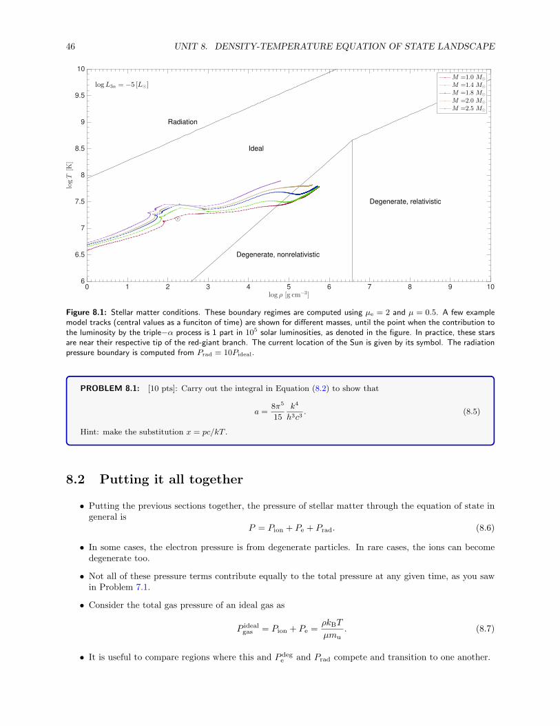
Figure 8.1: Stellar matter conditions. These boundary regimes are computed using µe = 2 and µ = 0.5. A few examplemodel tracks (central values as a funciton of time) are shown for different masses, until the point when the contribution tothe luminosity by the triple−α process is 1 part in 105 solar luminosities, as denoted in the figure. In practice, these starsare near their respective tip of the red-giant branch. The current location of the Sun is given by its symbol. The radiationpressure boundary is computed from Prad = 10Pideal.
PROBLEM 8.1: [10 pts]: Carry out the integral in Equation (8.2) to show that
a =8π5
15
k4
h3c3. (8.5)
Hint: make the substitution x = pc/kT .
8.2 Putting it all together
• Putting the previous sections together, the pressure of stellar matter through the equation of state ingeneral is
P = Pion + Pe + Prad. (8.6)
• In some cases, the electron pressure is from degenerate particles. In rare cases, the ions can becomedegenerate too.
• Not all of these pressure terms contribute equally to the total pressure at any given time, as you sawin Problem 7.1.
• Consider the total gas pressure of an ideal gas as
P idealgas = Pion + Pe =
ρkBT
µmu. (8.7)
• It is useful to compare regions where this and P dege and Prad compete and transition to one another.

8.2. PUTTING IT ALL TOGETHER 47
• First consider where an ideal gas transitions to a degenerate nonrelativistic one. Equating Equa-tion (7.10) and Equation (8.7) gives
ρ
µ5/2e
=
(
kBCµmu
)3/2
T 3/2, (8.8)
where C is the constant prefactor in Equation (7.10) .
• For large densities or low temperatures, i.e., when ρ T−3/2 > const, the gas is dominated by degeneratepressure. This is shown by the line of a slope of 2/3 in Figure 8.1.
• When electron speeds become relativistic, Equation (7.13) becomes appropriate, and when equatedwith the ideal gas pressure yields
ρ
µ4e
=
(
kBDµmu
)3
T 3, (8.9)
where D is the constant prefactor in Equation (7.13).
• This is shown in Figure 8.1 with the line of slope 1/3 at high temperature and density.
• In the degenerate regime, the transition from non- to relativistic is found by equating Equation (7.10)and Equation (7.13), which is independent of temperature (since these are completely degeneratesystems):
ρ
µe=
(
D
C
)3
. (8.10)
This is given in the figure by the vertical line.
• Finally, we can determine where radiation pressure starts to exceed ideal gas pressure. We use Equa-tion (8.3) to find
ρ
µ=
1
3
amu
kBT 3. (8.11)
• In Figure 8.1 this is shown by the line at the bottom right of slope 1/3.

48 UNIT 8. DENSITY-TEMPERATURE EQUATION OF STATE LANDSCAPE
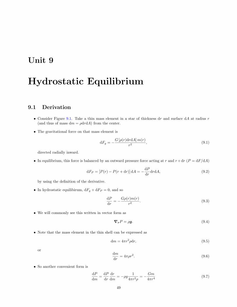
Unit 9
Hydrostatic Equilibrium
9.1 Derivation
• Consider Figure 9.1. Take a thin mass element in a star of thickness dr and surface dA at radius r(and thus of mass dm = ρdrdA) from the center.
• The gravitational force on that mass element is
dFg = −G [ρ(r)drdA]m(r)
r2, (9.1)
directed radially inward.
• In equilibrium, this force is balanced by an outward pressure force acting at r and r+dr (P = dF/dA)
dFP = [P (r)− P (r + dr)] dA = −dP
drdrdA, (9.2)
by using the definition of the derivative.
• In hydrostatic equilibirum, dFg + dFP = 0, and so
dP
dr= −Gρ(r)m(r)
r2. (9.3)
• We will commonly see this written in vector form as
∇rP = ρg. (9.4)
• Note that the mass element in the thin shell can be expressed as
dm = 4πr2ρdr, (9.5)
ordm
dr= 4πρr2. (9.6)
• So another convenient form is
dP
dm=
dP
dr
dr
dm= −ρg 1
4πr2ρ= − Gm
4πr4(9.7)
49
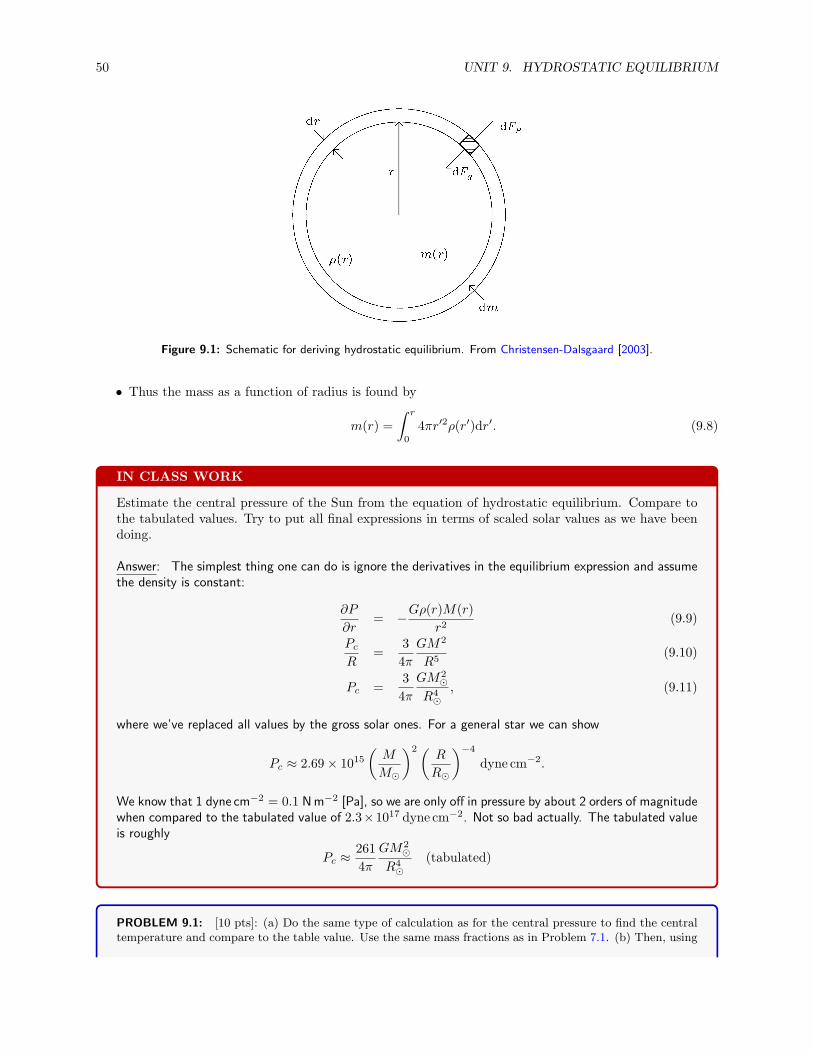
50 UNIT 9. HYDROSTATIC EQUILIBRIUM
Figure 9.1: Schematic for deriving hydrostatic equilibrium. From Christensen-Dalsgaard [2003].
• Thus the mass as a function of radius is found by
m(r) =
∫ r
0
4πr′2ρ(r′)dr′. (9.8)
IN CLASS WORK
Estimate the central pressure of the Sun from the equation of hydrostatic equilibrium. Compare tothe tabulated values. Try to put all final expressions in terms of scaled solar values as we have beendoing.
Answer: The simplest thing one can do is ignore the derivatives in the equilibrium expression and assumethe density is constant:
∂P
∂r= −Gρ(r)M(r)
r2(9.9)
Pc
R=
3
4π
GM2
R5(9.10)
Pc =3
4π
GM2⊙
R4⊙
, (9.11)
where we’ve replaced all values by the gross solar ones. For a general star we can show
Pc ≈ 2.69× 10¹⁵(
M
M⊙
)2(R
R⊙
)−4
dyne cm−2.
We know that 1 dyne cm−2 = 0.1 Nm−2 [Pa], so we are only off in pressure by about 2 orders of magnitudewhen compared to the tabulated value of 2.3×10¹⁷ dyne cm−2. Not so bad actually. The tabulated valueis roughly
Pc ≈261
4π
GM2⊙
R4⊙
(tabulated)
PROBLEM 9.1: [10 pts]: (a) Do the same type of calculation as for the central pressure to find the centraltemperature and compare to the table value. Use the same mass fractions as in Problem 7.1. (b) Then, using

9.1. DERIVATION 51
the expressions you now have for the gas pressure and temperature, show that we can ignore the radiationpressure for the Sun in the core. I.e., show that PR/PG ≈ c(M/M⊙)
2, where c is a smallish number. Try toput all final expressions in terms of scaled solar values as we have been doing.
EXAMPLE PROBLEM 9.1: In Equation (9.11) we found a cheap and dirty estimate of the central pressure.Now, using Equations (9.3) and (9.6), we can find a lower bound for the pressure at the center of the Sun.First we need an expression for dP/dm and then integrate from core to surface. Making a simple assumptionin the integrand allows you to argue this is really a lower limit. Compare again to the previous result of thein class problem by expressing your final answer in terms of
Pc = const×GM2
⊙
R4⊙
, (9.12)
where the constant is really the key quantity in your computation.
Answer:dP
dm=
dP
dr
dr
dm= −
Gm
4πr4.
We can take simply that r = R⊙. Integrate both sides from the center to the surface:
∫ m=M⊙
m=0
dP = P (M⊙)− P (0) = −
∫ m=M⊙
m=0
Gm
4πr4dm.
To obtain an absolute lower limit, let’s just take r = R⊙, it’s the simplest thing we can do and we know it makesthe overall value the smallest. Then
P (M⊙)− P (0) = −G
4πR4⊙
∫ m=M⊙
m=0
m dm =1
8π
GM2⊙
R4⊙
< P (0).
This gives
Pc ≈ 4.5× 10¹⁴(
M
M⊙
)2 (
R
R⊙
)−4
dyne cm−2,
below the value in the table and below the one found before. But it is a lower limit. It is very interesting that thislimit is valid for any star in hydrostatic equilibrium, independent of equation of state or energy production.
EXAMPLE PROBLEM 9.2: Let’s improve the lower limit now (i.e., make it a bit larger). All that is neededis to assume a mean density that is a decreasing function of r such as
ρ(r) =m
4πr3/3.
Use this at the right step in Problem 9.1 to get a new lower limit, again expressed as
Pc = const×GM2
⊙
R4⊙
.
Answer: Picking up where we left off by solving for r as a function of the density and mass gives
P (0) >G
4π
∫ M⊙
0
m
(3m/4πρ)4/3dm =
G
4π
(
4πρ
3
)4/3 ∫ M⊙
0
m−1/3dm =G
4π
(
4πρ
3
)4/33
2M
2/3⊙ =
3
8π
GM2⊙
R4⊙
.
In the last step we simply allowed the mean density to be the gross solar values. This gives us a new value 3 timeslarger than the previous one, but still twice as small as that in Equation (9.11).
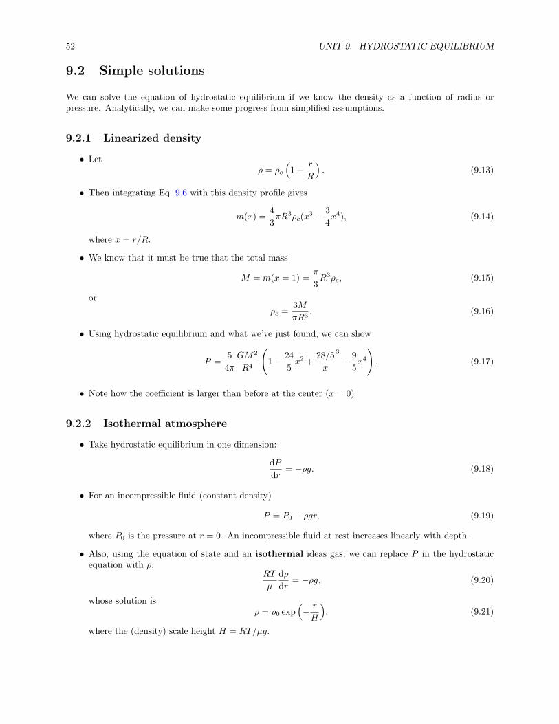
52 UNIT 9. HYDROSTATIC EQUILIBRIUM
9.2 Simple solutions
We can solve the equation of hydrostatic equilibrium if we know the density as a function of radius orpressure. Analytically, we can make some progress from simplified assumptions.
9.2.1 Linearized density
• Letρ = ρc
(
1− r
R
)
. (9.13)
• Then integrating Eq. 9.6 with this density profile gives
m(x) =4
3πR3ρc(x
3 − 3
4x4), (9.14)
where x = r/R.
• We know that it must be true that the total mass
M = m(x = 1) =π
3R3ρc, (9.15)
or
ρc =3M
πR3. (9.16)
• Using hydrostatic equilibrium and what we’ve just found, we can show
P =5
4π
GM2
R4
(
1− 24
5x2 +
28/5
x
3
− 9
5x4
)
. (9.17)
• Note how the coefficient is larger than before at the center (x = 0)
9.2.2 Isothermal atmosphere
• Take hydrostatic equilibrium in one dimension:
dP
dr= −ρg. (9.18)
• For an incompressible fluid (constant density)
P = P0 − ρgr, (9.19)
where P0 is the pressure at r = 0. An incompressible fluid at rest increases linearly with depth.
• Also, using the equation of state and an isothermal ideas gas, we can replace P in the hydrostaticequation with ρ:
RT
µ
dρ
dr= −ρg, (9.20)
whose solution isρ = ρ0 exp
(
− r
H
)
, (9.21)
where the (density) scale height H = RT/µg.
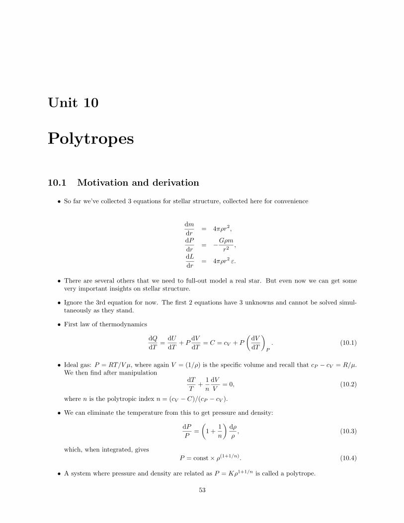
Unit 10
Polytropes
10.1 Motivation and derivation
• So far we’ve collected 3 equations for stellar structure, collected here for convenience
dm
dr= 4πρr2,
dP
dr= −Gρm
r2,
dL
dr= 4πρr2 ε.
• There are several others that we need to full-out model a real star. But even now we can get somevery important insights on stellar structure.
• Ignore the 3rd equation for now. The first 2 equations have 3 unknowns and cannot be solved simul-taneously as they stand.
• First law of thermodynamics
dQ
dT=
dU
dT+ P
dV
dT= C = cV + P
(
dV
dT
)
P
. (10.1)
• Ideal gas: P = RT/V µ, where again V = (1/ρ) is the specific volume and recall that cP − cV = R/µ.We then find after manipulation
dT
T+
1
n
dV
V= 0, (10.2)
where n is the polytropic index n = (cV − C)/(cP − cV ).
• We can eliminate the temperature from this to get pressure and density:
dP
P=
(
1 +1
n
)
dρ
ρ, (10.3)
which, when integrated, gives
P = const× ρ(1+1/n). (10.4)
• A system where pressure and density are related as P = Kρ1+1/n is called a polytrope.
53

54 UNIT 10. POLYTROPES
• For an adiabatic change C = 0, n = 1/(γ − 1), and
P = Kργ , (10.5)
where γ = cP /cV .
• This is very useful because we can now get radial profiles of P (r), T (r),m(r) and ρ(r).
10.2 Lane-Emden equation
• Take hydrostatic equilibrium, divide by density, multiply by r2, and use the mass gradient equation:
d
dr
(
r2
ρ
dP
dr
)
= −4πGρr2. (10.6)
• Consider the polytropic equation of state
d
dr
(
r2Kγργ−2 dρ
dr
)
= −4πGρr2. (10.7)
• Use polytropic index n and let the density be rewritten as a unitless quantity θ by
ρ
ρc= θn, (10.8)
where ρc is the central density of a model.
• Then(n+ 1)Kρ
1/n−1c
4πG
1
r2d
dr
(
r2dθ
dr
)
= −θn. (10.9)
• Let the coefficient (of units distance squared) be α2, where
α =
[
(n+ 1)Kρ1/n−1c
4πG
]1/2
=
[
(n+ 1)Pc
4πGρ2c
]1/2
. (10.10)
(You might want to prove to yourself the above is true and the unit is distance).
• We then scale the radial coordinate
r = αξ. (10.11)
• Then1
ξ2d
dξ
(
ξ2dθ
dξ
)
= −θn. (10.12)
This is known as the Lane-Emden equation.
• Boundary conditions at the center must satisfy (noting Equation (10.8))
θ(ξ) = 1 at ξ = 0, (10.13)
dθ
dξ= 0 at ξ = 0. (10.14)
• Define the surface as
θ(ξ) = 0 at ξ = ξ1. (10.15)
10.3. POLYTROPE SOLUTIONS 55
10.3 Polytrope solutions
• In what follows, a subscript n denotes the label of the polytropic index, whereas the supercript n isthe quantity raised to the nth power.
• Assume a solution θn(ξ) can be found to Equation (10.12) for a given index n.
• Then the radius of the model is
R =
[
(n+ 1)Kρ1/n−1c
4πG
]1/2
ξ1 = αξ1. (10.16)
• The mass interior to m(ξ) is
m(ξ) =
∫ αξ
0
4πr′2ρ dr′ = 4πα3ρc
∫ ξ
0
ξ′2θn dξ′ (10.17)
= −4πα3ρc
∫ ξ
0
d
dξ′
(
ξ′2dθ
dξ′
)
dξ′ (10.18)
= −4πα3ρcξ2 dθ
dξ(10.19)
m(ξ) = −4π[
(n+ 1)K
4πG
]3/2
ρ(3−n)/2nc ξ2
dθ
dξ. (10.20)
• The total mass is
M = −4π[
(n+ 1)K
4πG
]3/2
ρ(3−n)/2nc
(
ξ2dθ
dξ
)
ξ=ξ1
. (10.21)
• Inspecting the mass and radius relations, the constant K is
K = NGM (n−1)/nR(3−n)/n, (10.22)
where
N =(4π)1/n
n+ 1
[
−ξ(n+1)/(n−1)1
(
dθ
dξ
)
ξ=ξ1
](1−n)/n
. (10.23)
• It is interesting to point out here that if K is known from some equation of state, then one can deriveexplicit mass-radius relationships. If that is not the case, then mass and radius must be predefined.More about this later.
• Mean density of model
ρ =M
V= − 3
ξ1
(
dθ
dξ
)
ξ=ξ1
ρc. (10.24)
• Central density is then
ρc = −ξ13
(
dθ
dξ
)−1
ξ=ξ1
M
4/3πR3. (10.25)
• Central pressure
Pc = Kρ(n+1)/nc , (10.26)
or
Pc = WnGM2
R4, (10.27)

56 UNIT 10. POLYTROPES
where
Wn =
[
4π(n+ 1)
(
dθ
dξ
)2
ξ=ξ1
]−1
. (10.28)
Note that this is the coefficient we were computing in some simple example problems (cf. Equa-tion (9.11)).
• So pressure throughout model isP = Pcθ
n+1. (10.29)
• For the temperature, assume an ideal gas with µ constant, then
T = Tcθ, (10.30)
where
Tc = ΘGMµmu
kBR, (10.31)
and
Θ =
[
−(n+ 1)ξ1
(
dθ
dξ
)
ξ=ξ1
]−1
. (10.32)
Again here, this coefficient is a number obtained through simpler means using only hydrostatic equi-librium (cf. Problem 9.1).
• The distribution of mass in a polytrope can be obtained easily (see Equation (10.20) and Equa-tion (10.21))
q =m
M=
(
ξ2dθ
dξ
)(
ξ2dθ
dξ
)−1
ξ=ξ1
. (10.33)
• Only 3 analytical solutions of the Lane-Emden equation are possible:
n = 0 ; θ0 = 1− 1
6ξ2, (10.34)
n = 1 ; θ1 =sin ξ
ξ, (10.35)
n = 5 ; θ5 = (1 +1
3ξ2)−1/2. (10.36)
COMPUTER PROBLEM 10.1: [40 points]: Solve the Lane-Emden Equation (10.12) numerically with thetwo boundary conditions using your method of choice for your assigned index n.
What to do
• To solve the 2nd-order nonlinear differential equation, which is a difficult task to do as is, the firstthing you will need to do is to make a substitution to generate 2 first-order differential equations, ascan always be done. A suitable choice may be to let y = θ and z = dθ/dξ = y′. You’ll then be able tohave an equation for y′ and one for z′.
• Next you need to choose your solver. You can treat this as a boundary-value problem, in which case amethod like Newton-Rhapson can be used. Fancy software like IDL, Python, and MATLAB have built-inboundary value algorithms, but can be tricky to implement in some cases. Perhaps a better option is touse such languages and code your own algorithm, perhaps implementing a “shooting method,” whichtreats the problem as an initial-value problem. You “shoot” from the center, say, and work your wayout to the end of the model using an integrator. A common and very handy integrator is Runge-Kutta.I’d suggest this method (shooting) because you don’t need any sophisticated algorithms and it works!But it’s your choice. A 4th-order Runge-Kutta is sufficient for this problem if you choose to do so.There’s lots of information on this in the Numerical Recipes book, for example. If you do this, make

10.3. POLYTROPE SOLUTIONS 57
sure you verify through testing that you choose the proper grid spacing.
• You have to be a little careful about how you treat the center of the model since there is a possibledivergence in your equation(s) (as should be apparent already). If one expands the Lane-Emdenequation about the origin, it can be shown that
θn(ξ) ≃ 1−1
6ξ2 +
n
120ξ4 −
n(8n− 5)
15120ξ6 + . . . (10.37)
You can use this approximation to set your first values for y and z (if you choose to solve the problemwith this class of methods) by taking a very small, but finite, starting ξ. Then just run it until youcross the first zero in θn. Make sure your grid is sufficiently fine so the solution is smooth.
What to hand in
(a) You will solve for a polytrope of given index n, assigned in the table. You will provide the instructorthe values (including 3 decimal places!) you find for the table columns for your n only. For the last 3columns in the table, compute those values for 1 solar mass, 1 solar radius, and composition X = 0.7 andZ = 0.02. We’ll fill the table in together when finished. Also provide a copy of your code. [15 pts]
(b) Plot the following quantities on a single full-page plot with appropriate labels and clearly distinguishablelines: θn(ξ), θnn(ξ), θn+1
n (ξ), and q(ξ). What do each of the 4 quantities that you are showing herephysically correspond to? [10 pts]
(c) Plot your model on a temperature-density (T − ρ) plot, as in Figure 8.1 (you don’t need to plot theboundary lines for different equations of state). Then overplot one of your MESA solar mass models,perhaps the one from Computer Problem 0 (the one found at the end of the MESA notes on the coursewebpage). If you didn’t save the density or temperature interior profile, it’s quick to rerun MESA agaginwith those quantities included. [5 pts]
(d) Derive those first 4 terms of the expansion in Equation (10.37). Hint: First show or explain that if θ(ξ)is a solution of the Lane-Emden equation, then so must θ(−ξ). This motivates you to try a solution ofthe form below of even powers which you can plug into the Lane-Emden equation:
θ(ξ) = C0 + C2ξ2 + C4ξ
4 + C6ξ6 + . . . (10.38)
Don’t forget to use any boundary conditions you may need. [10 pts]
n Name ξ1 ρc/ρ Nn Wn Θn ρc Pc Tc
[g cm−3] [dyne cm−2] [K]
0.0 –0.5 Hannah1.0 –1.5 Harrison2.0 Rogelio2.25 Annie2.5 Ali2.75 Audrey3.0 Mark3.25 Alexander3.5 Kelly3.75 Farhan4.0 Bryson4.25 Matt4.5 Oana4.75 Manny5.0 –
58 UNIT 10. POLYTROPES
10.4 Usefulness of polytropes
• First note that unless K is fixed by a known equation of state (like it is for degenerate gases and a fewother cases), then one needs to provide a value of n, M , and R to get physical values for the interiorproperties.
• A degenerate gas is a case where K is fixed by the equation of state. Recall the non-relativistic casein Equation (7.10):
Pe = 1.0036× 10¹³(
ρ
µe
)5/3
dyne cm−2.
• The exponent on density implies n = 3/2.
• Using the expression for K in Equation (10.22) along with the necessary computed values gives
K = 2.477× 10¹⁴(
M
M⊙
)1/3R
R⊙
. (10.39)
• This yields a mass-radius relationship
M
M⊙
≈ 2.08× 10⁻⁶
(
2
µe
)5(R
R⊙
)−3
. (10.40)
Note how this implies that adding mass decreases the star’s radius.
• White dwarfs are measured to have masses around 0.6M⊙. For completely ionized gas, µe = 2, andthis gives a radius of about R ≈ 0.015R⊙, which is about the radius of the Earth.
• In deriving Equation (7.10) we could have substituted the mass of the neutron instead of the electron.Neutrons can become degenerate in special cases too. Then taking µe = 1, the neutron star equivalentof Equation (10.40) is
M
M⊙
≈ 5× 10⁻¹⁵
(
R
R⊙
)−3
. (10.41)
• For a 1M⊙ star, we find R ≈ 10 km.
• For relativistic electrons, we had from Equation (7.13)
Pe = 1.243× 10¹⁵(
ρ
µe
)4/3
dyne cm−2.
• This now implies a polytropic index n = 3. Using the proper values for this case gives
K = 3.841× 10¹⁴(
M
M⊙
)2/3
, (10.42)
or, the relation (independent of radius)
M
M⊙
= 1.456
(
2
µe
)2
. (10.43)
• This is the Chandrasekhar limiting mass for a degenerate, relativistic electron gas. We’ll come back tothis again discussing late-stage evolution.
• Another interesting insight is for radiation pressure.
10.4. USEFULNESS OF POLYTROPES 59
• Consider the case for an ideal gas where radiation pressure is also contributing. Recall Equation (12.1)
P =Rg
µρT +
1
3aT 4 =
Rg
µβρT,
where β = Pgas/P is assumed constant throughout the star.
• If we write this as
Prad =1− β
βPgas =
1− β
β
ρRg
µT =
1
3aT 4, (10.44)
then we can solve for T , which gives
T =
(
3Rg
aµ
1− β
β
)1/3
ρ1/3. (10.45)
• Using this to plug back into the total pressure P , we can find
P =
(
3R4g
aµ4
)1/3(
1− β
β4
)1/3
ρ4/3 = Kρ4/3, (10.46)
which demonstrates this is an n = 3 polytrope.
• Here, K is again a free parameter given some value of β. But we also have another expression for Kfrom Eq. (10.22).
• Equating those 2 Ks and using the right values for n = 3 gives
1− β
β4= 0.002996µ4
(
M
M⊙
)2
. (10.47)
• This shows, as expected, that more massive stars have larger contributions from radiation pressure.
• For µ2M/M⊙ = 1, β = 0.997. But for µ2M/M⊙ = 50, β ≈ 0.5.
• One can also look at the temperature using the above result to find
T = 4.62× 10⁶ βµ
(
M
M⊙
)2/3
ρ1/3. (10.48)
• Finally, consider the Sun.
• It is apparent from the polytrope solutions (Table ??) that Θn does not change much with n, so ourapproximation for the central temperature found in Problem 9.1 is quite good, where we effectivelyfound that Θ = 1. The numerical central temperature is Tc = 1.57× 10⁷ K.
• We see that other solutions however vary quite widely for different indices. For example, The Wn canbe directly compared with our prior estimates of central pressure in Section 9.1. For the Sun we foundthat the constant is about 261/4π ≈ 21, with total numerical value Pc = 2.34× 10¹⁷ dyne cm2 . This isthe first piece of evidence that the Sun is well described by a n = 3 polytrope.
• We also know the Sun’s central density is about ρc = 153 g cm−3, and ratio with mean density 153/1.4 ≈110.
• All of these comparisons point to the Sun being somewhere between n = 3.0 − 3.5, at least in thecentral regions.
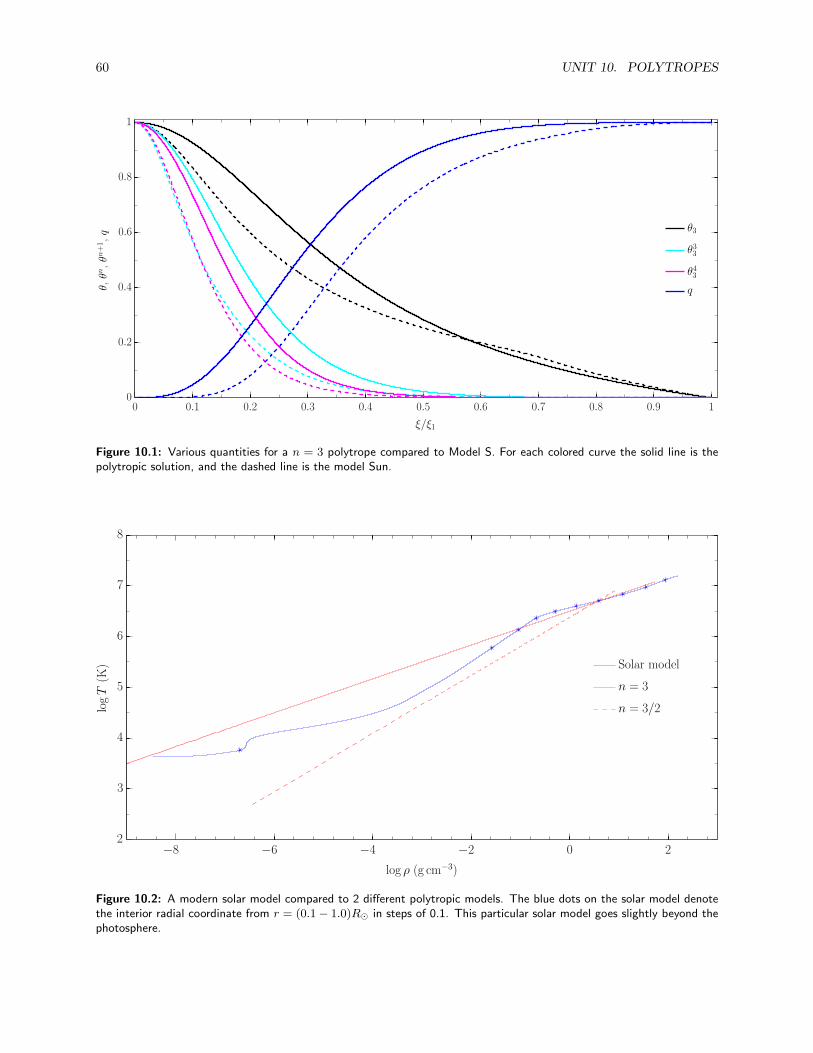
60 UNIT 10. POLYTROPES
q
θ43
θ33
θ3
θ,θn,θn
+1,q
ξ/ξ1
0 0.1 0.2 0.3 0.4 0.5 0.6 0.7 0.8 0.9 10
0.2
0.4
0.6
0.8
1
Figure 10.1: Various quantities for a n = 3 polytrope compared to Model S. For each colored curve the solid line is thepolytropic solution, and the dashed line is the model Sun.
n = 3/2
n = 3
Solar model
logT(K
)
log ρ (g cm−3)
−8 −6 −4 −2 0 22
3
4
5
6
7
8
Figure 10.2: A modern solar model compared to 2 different polytropic models. The blue dots on the solar model denotethe interior radial coordinate from r = (0.1− 1.0)R⊙ in steps of 0.1. This particular solar model goes slightly beyond thephotosphere.
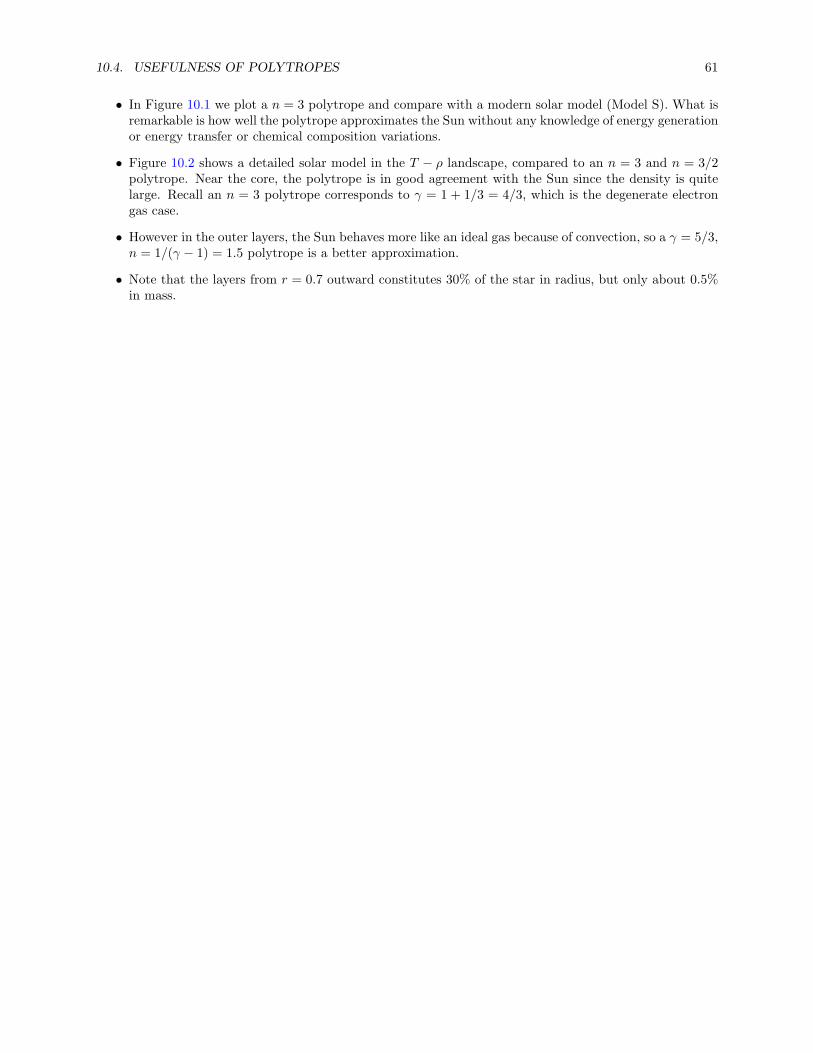
10.4. USEFULNESS OF POLYTROPES 61
• In Figure 10.1 we plot a n = 3 polytrope and compare with a modern solar model (Model S). What isremarkable is how well the polytrope approximates the Sun without any knowledge of energy generationor energy transfer or chemical composition variations.
• Figure 10.2 shows a detailed solar model in the T − ρ landscape, compared to an n = 3 and n = 3/2polytrope. Near the core, the polytrope is in good agreement with the Sun since the density is quitelarge. Recall an n = 3 polytrope corresponds to γ = 1 + 1/3 = 4/3, which is the degenerate electrongas case.
• However in the outer layers, the Sun behaves more like an ideal gas because of convection, so a γ = 5/3,n = 1/(γ − 1) = 1.5 polytrope is a better approximation.
• Note that the layers from r = 0.7 outward constitutes 30% of the star in radius, but only about 0.5%in mass.

62 UNIT 10. POLYTROPES
Unit 11
Thermodynamics of an Ideal Gas
11.1 First law of thermodynamics
• Here we consider quasistatic changes to the state of a nondegenerate gas to understand its thermody-namic properties. Thermodynamics are “responses” of a gas to perturbations.
• As already stated, the internal energy per unit volume of an ideal gas is
u =3
2nkBT =
3
2
ρkBT
µmp=
3
2P. (11.1)
• Therefore the average energy per particle is 3/2kBT . Example problem 6.1 arrived at this in a slightlydifferent way.
• We define the specific volume V as the volume corresponding to unit mass, V = volume/mass = 1/ρ.The specific internal energy is the internal energy per unit mass U = u/ρ:
U =3
2
kBT
µmu. (11.2)
• Remember that the first law of thermodynamics tells us that we can (slowly) change the internal energyof gas by adding heat or doing work:
dU = dQ+ dW, (11.3)
where U is the specific internal energy of the matter, V is the specific volume it occupies, and dQ issome amount of heat added to it.
• The work done is to contract or expand it, so dW = −PdV .
• The more proper form for our use is
dQ = dU + PdV. (11.4)
This heat partly changes the internal energy of the matter and also potentially changes the volume.
• Keeping the volume constant the first law of thermodynamics becomes
cV =
(
dQ
dT
)
V
=dU
dT=
3
2
kBµmu
=3
2
R
µ. (11.5)
This is the specific heat at constant volume.
63

64 UNIT 11. THERMODYNAMICS OF AN IDEAL GAS
• Now consider how to arrive at an expression for constant pressure. Rewrite the first law
dQ = dU + PdV + V dP − V dP = dU − V dP + d(PV ), (11.6)
d(PV ) = d(NkBT ) =kBµmu
dT, (11.7)
remembering that N = nV = n/ρ = ρ/(µmuρ) = 1/µmu.
• Then
dQ = dU − V dP +kBµmp
dT =5
2
kBµmu
dT − V dP, (11.8)
by using Equation (11.2).
• Therefore the specific heat at constant pressure is
cP =5
2
kBµmu
=5
2
R
µ.. (11.9)
Note that cP − cV = R/µ.
• Note also the ratio of specific heats, γ = cP /cV , which for an ideal gas γ = 5/3 since the specific heatsare constants.
11.2 Adiabatic process
• An adiabatic process is one in which no heat is added to the gas (dQ = 0).
• In this special case, we can find expressions relating changes in P and V . Using the above expressionswe can show
cV
(
dP
P+
dV
V
)
= − kBµmp
dV
V= (cV − cP )
dV
V. (11.10)
• Finally we see thatdP
P= −γ dV
V= γ
dρ
ρ= − γ
1− γ
dT
T. (11.11)
• Since γ is constant in this case, such equations can be readily integrated to yield relations such asPV γ = const.
• Using the ideal gas law we can also write (just in terms of P , T , and V ):(
∂ lnP
∂ lnV
)
s
= −γ ≡ −Γ1 (11.12)
(
∂ lnP
∂ ln ρ
)
s
= γ ≡ Γ1 (11.13)
(
∂ lnP
∂ lnT
)
s
=γ
γ − 1≡ Γ2
Γ2 − 1(11.14)
(
∂ lnT
∂ lnV
)
s
= 1− γ ≡ 1− Γ3. (11.15)
(
∂ lnT
∂ ln ρ
)
s
= γ − 1 ≡ Γ3 − 1. (11.16)
• The s means adiabatic, or at constant entropy, where dQ = TdS.
• The connection between Eq. (11.12) and (11.13) is clear from the specific volume definition. Similarlyfor Eq. (11.15) and (11.16).
11.2. ADIABATIC PROCESS 65
EXAMPLE PROBLEM 11.1: Derive the 2 equations (11.10) and (11.11).
Answer: Begin with Equation (11.7) rewritten here:
PdV + V dP =kBµmp
dT.
For adiabatic processes, the first law gives us that
cV dT = −PdV,
so that we have
PdV + V dP = −kBµmp
1
cVPdV.
Now divide through by PV and recall the relationship between the 2 specific heats to find
cV
(
dV
V+
dP
P
)
= (cV − cP )dV
V.
Collecting terms givesdP
P= −γ
dV
V= γ
dρ
ρ.
The term with the log is just a different way of rewriting the above equation, such as
d lnP
d ln ρ= γ.
To get the term with P and T , remember that with the ideal gas law, P ∼ ρT (forget the constants n or k; they’lldrop out in the end). So using the product rule,
dP = Tdρ+ ρdT,
and then divide by P, multiply by γ, and use the ideal gas law. We find
γdρ
ρ= γ
(
dP
P−
dT
T
)
,
and collecting terms can then give you Equation (11.14). Using the ideal gas law again with T and ρ will give youEquation (11.15).

66 UNIT 11. THERMODYNAMICS OF AN IDEAL GAS

Unit 12
Thermodynamics with Photons
12.1 Mixture of ideal gas and radiation: pressure effects
• It should be noted that we have been considering an ideal gas made up of particles only. When radiationis present along with the gas in thermodynamic equilibrium, the photons can cause two changes: (1)a radiation pressure; and (2) ionization effects (see Sec. 12.2). In this case, the adiabatic exponents inEqs. (11.12-11.15) are not constant anymore, nor are they all equal.
• Considering this mixture, the total pressure is
P = Pgas + Prad =ρkBT
µmu+
1
3aT 4, (12.1)
and specific internal energy density
U =3
2
kBT
µmu+ aT 4V. (12.2)
• Since the specific energy depends on volume and temperature U(T, V ), quasistatic changes to it in thefirst law of thermodynamics yields
dQ =
(
∂U
∂T
)
V
dT +
(
∂U
∂V
)
T
dV + PdV. (12.3)
• Using the expression for the specific energy and pressure then gives
dQ =
(
4aT 3V +3
2
kBµmu
)
dT +
(
4
3aT 4 +
kBT
µmuV
)
dV. (12.4)
• For an adiabatic process, this equation gives the thermodynamic response to changes in temperatureand volume. It can then be nicely rewritten
(
12Prad +3
2Pgas
)
dT
T+ (4Prad + Pgas)
dV
V= 0. (12.5)
• To evaluate expressions as in Equations (11.12)-(11.15), it’s also useful to have a pressure differentialterm. Using Equation (12.1) we can write
dP =
(
4
3aT 4 +
RT
µV
)
dT
T− R
µ
T
V
dV
V,
= (4Prad + Pgas)dT
T− Pgas
dV
V. (12.6)
67
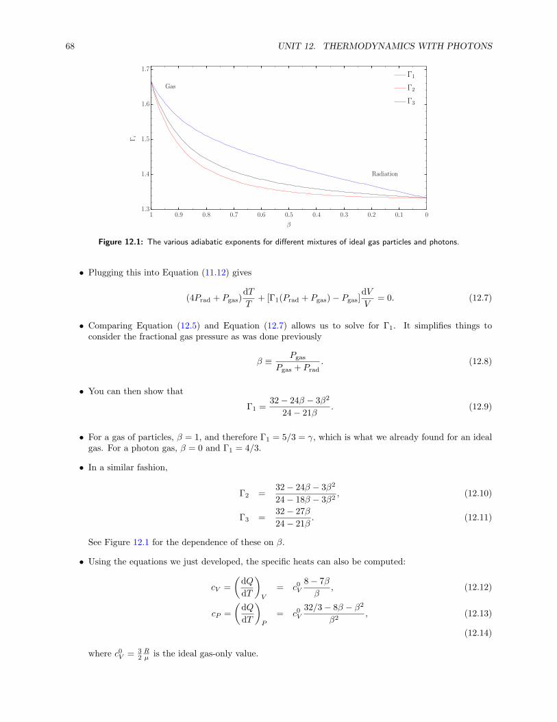
68 UNIT 12. THERMODYNAMICS WITH PHOTONS
Radiation
Gas
Γi
β
Γ3
Γ2
Γ1
00.10.20.30.40.50.60.70.80.911.3
1.4
1.5
1.6
1.7
Figure 12.1: The various adiabatic exponents for different mixtures of ideal gas particles and photons.
• Plugging this into Equation (11.12) gives
(4Prad + Pgas)dT
T+ [Γ1(Prad + Pgas)− Pgas]
dV
V= 0. (12.7)
• Comparing Equation (12.5) and Equation (12.7) allows us to solve for Γ1. It simplifies things toconsider the fractional gas pressure as was done previously
β ≡ Pgas
Pgas + Prad. (12.8)
• You can then show that
Γ1 =32− 24β − 3β2
24− 21β. (12.9)
• For a gas of particles, β = 1, and therefore Γ1 = 5/3 = γ, which is what we already found for an idealgas. For a photon gas, β = 0 and Γ1 = 4/3.
• In a similar fashion,
Γ2 =32− 24β − 3β2
24− 18β − 3β2, (12.10)
Γ3 =32− 27β
24− 21β. (12.11)
See Figure 12.1 for the dependence of these on β.
• Using the equations we just developed, the specific heats can also be computed:
cV =
(
dQ
dT
)
V
= c0V8− 7β
β, (12.12)
cP =
(
dQ
dT
)
P
= c0V32/3− 8β − β2
β2, (12.13)
(12.14)
where c0V = 32Rµ is the ideal gas-only value.

12.2. MIXTURE OF IDEAL GAS AND RADIATION: IONIZATION EFFECTS 69
Neutral
Ionized
logT[K]
log ρ [g cm−3]
−10 −8 −6 −4 −2 0 23.5
4
4.5
5
5.5
6
Figure 12.2: Ionization of a pure H gas using Equation (12.19). The lower line represents the state at 50% ionization,while the upper is for 99%.
• Note that the ratio of specific heats givescPcV
=Γ1
β, (12.15)
which makes sense in the appropriate limits, reducing to what we found before.
• The same procedure can be carried out for mixtures of some degenerate gas too.
12.2 Mixture of ideal gas and radiation: ionization effects
• As mentioned at the beginning of this section, the other consideration is the ionization of the gas thatradiation produces, which has profound effects on the thermodynamic state of the gas.
• Let’s just consider a hydrogen gas for simplicity in what follows.
• In general radiation causes ionization and subsequent recombination:
H+ + e− ←→ H0 + χH, (12.16)
where χH = 13.6 eV is the energy needed to ionize hydrogen. We will only consider the ground state.
• To measure the number densities of electrons (ne), ions (n+), and neutral H (n0) in thermodynamicequilibrium, we employ the tools we used in Sec. 6.1 using a Boltzmann distribution.
• After taking into account the appropriate degeneracy factors and energy levels and chemical potentials,we can form the ratio n+ne/n
0 using Equation (6.12) and obtain the Saha equation for a pure hydrogengas
n+ne
n0=
(
2πmekBh2
)3/2
T 3/2e−χH/kT . (12.17)
• We constrain the system to have charge neutrality, ne = n+ and nucleon number density n+ +n0 = n.Then we define the fraction of ionization
y =ne
n=
n+
n, (12.18)
as we did in Equation (5.16).
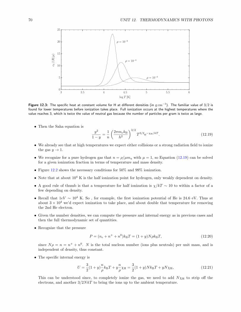
70 UNIT 12. THERMODYNAMICS WITH PHOTONS
ρ = 10−2
ρ = 10−4
ρ = 10−6
c V/(R/µ
)
log T [K]
3 3.5 4 4.5 5 5.5 60
5
10
15
20
25
Figure 12.3: The specific heat at constant volume for H at different densities (in g cm−3). The familiar value of 3/2 isfound for lower temperatures before ionization takes place. Full ionization occurs at the highest temperatures where thevalue reaches 3, which is twice the value of neutral gas because the number of particles per gram is twice as large.
• Then the Saha equation is
y2
1− y=
1
n
(
2πmekBh2
)3/2
T 3/2e−χH/kT . (12.19)
• We already see that at high temperatures we expect either collisions or a strong radiation field to ionizethe gas y → 1.
• We recognize for a pure hydrogen gas that n = ρ/µmu with µ = 1, so Equation (12.19) can be solvedfor a given ionization fraction in terms of temperature and mass density.
• Figure 12.2 shows the necessary conditions for 50% and 99% ionization.
• Note that at about 104 K is the half ionization point for hydrogen, only weakly dependent on density.
• A good rule of thumb is that a temperature for half ionization is χ/kT ∼ 10 to within a factor of afew depending on density.
• Recall that 1eV ∼ 104 K. So , for example, the first ionization potential of He is 24.6 eV. Thus atabout 3 × 10⁴ we’d expect ionization to take place, and about double that temperature for removingthe 2nd He electron.
• Given the number densities, we can compute the pressure and internal energy as in previous cases andthen the full thermodynamic set of quantities.
• Recognize that the pressure
P = (ne + n+ + n0)kBT = (1 + y)NρkBT, (12.20)
since Nρ = n = n+ + n0. N is the total nucleon number (ions plus neutrals) per unit mass, and isindependent of density, thus constant.
• The specific internal energy is
U =3
2(1 + y)
n
ρkBT + y
n
ρχH =
3
2(1 + y)NkBT + yNχH, (12.21)
This can be understood since, to completely ionize the gas, we need to add NχH to strip off theelectrons, and another 3/2NkT to bring the ions up to the ambient temperature.

12.2. MIXTURE OF IDEAL GAS AND RADIATION: IONIZATION EFFECTS 71
Γ3
Γ2
Γ1
log T [K]
Γi
3 3.5 4 4.5 5 5.5 61
1.2
1.4
1.6
1.8
Figure 12.4: Adiabatic exponents for ionized H at a density of 10−4 g cm−3.
• From these expressions the specific heats can be computed from the appropriate differentials. SinceU = U(T, y), and cV = dU/dT , we get extra terms.
• It works out to be
cV =3
2NkB(1 + y)
[
1 +2
3D(y)
(
3
2+
χH
kBT
)2]
, (12.22)
where
D(y) =y(1− y)
(2− y)(1 + y). (12.23)
• Note that D(0) = D(1) = 0, so the specific heat only changes by 1 + y as the gas goes from neutralto fully ionized. But D is finite for intermediate values of y, thus bringing in contributions from theother terms.
• A few examples of cV are shown in Figure 12.3 for several densities.
• Finally, the adiabatic exponents can be computed in similar ways using the prior results and Eqs. (11.12)-(11.15).
• Their values for a density of 10−4 across the ionization fraction range is shown in Figure 12.4.
• The Γi all take their ideal gas values for full ionization and for complete neutrality.
• Where ionization occurs, the values decrease quickly, and then increase again as ionization completes.
• To understand this, consider adiabatic compression of the gas, and let’s focus on Γ3, which, accordingto Equation (11.15), relates the temperature and volume.
• Before ionization, we see the value of 5/3 for the neutral gas, which simply means it is heating upunder compression as T ∼ ρ2/3 ∼ V −2/3.
• When ionization starts to occur, the value decreases, and the temperature sensitivity on volume isweaker. The energy is used to ionize the gas, instead of heating it up as quickly.

72 UNIT 12. THERMODYNAMICS WITH PHOTONS
12.3 Useful ideal gas equations
Let’s collect many of the useful relationships:
P =ρRT
µ=
ρkBT
m(12.24)
Pρ−γ = const (12.25)
cs =
√
γRT
M=
√
γP
ρ(12.26)
CP − CV = R/µ (12.27)
CV =3
2
R
µ(12.28)
CP =5
2
R
µ(12.29)
U =
∫ M
0
CV T dm′ (12.30)
Unit 13
Energy Transport: Radiation
Energy liberated in stellar interiors is transferred to the surface by radiation, convection, and conduction.We are not considering here radiation from a stellar photosphere, only the movement of photons in stellarinteriors.
13.1 Basics
• The basic idea is that photons emitted in hot regions of a star are absorbed in cooler regions of a star,thus “transferring” energy from hot to cool.
• As we’ll soon see, the “efficiency” of this transfer will depend on the temperature gradient. A veryrough approximation of the gradient for the Sun is dT/dr ≈ (Tsurf − Tcore)/(rsurf − rcore) ≈ Tc/R⊙ ≈−2.25× 10⁻⁴ Kcm−1.
• Figure 13.1 shows this number compared to the “true” temperature gradient in the interior of the Sun.Clearly there is more physics taking place than we’ve considered so far.
• The efficiency of radiation will also depend on the ability of the photons to travel freely.
• Consider the luminosity roughly as the (total radiation energy stored in the star) divided by the (escapetime for photons).
• The radiation energy is the energy density of photons (Eq. 8.4), say, at the central temperature of thestar (the Sun in this case)
Eγ = aT 4c ·
4π
3R3
⊙. (13.1)
• For the photon escape time, let’s first consider that the Sun were completely transparent to photons.The time would then be R⊙/c = 2.32 s. The resulting luminosity would be quite large!
EXAMPLE PROBLEM 13.1: If we regard the Sun as a large cavity filled with photons, compute theluminosity by estimating the total energy stored in the radiation field and the Sun becoming completelytransparent. Express the luminosity in L⊙.
• More formally, the mean free path of photons can be expressed as
ℓph =1
κρ, (13.2)
where κ is some absorption coefficient (in units of cross section per unit mass) that will be given aphysical meaning later, and ρ is the mass density.
73
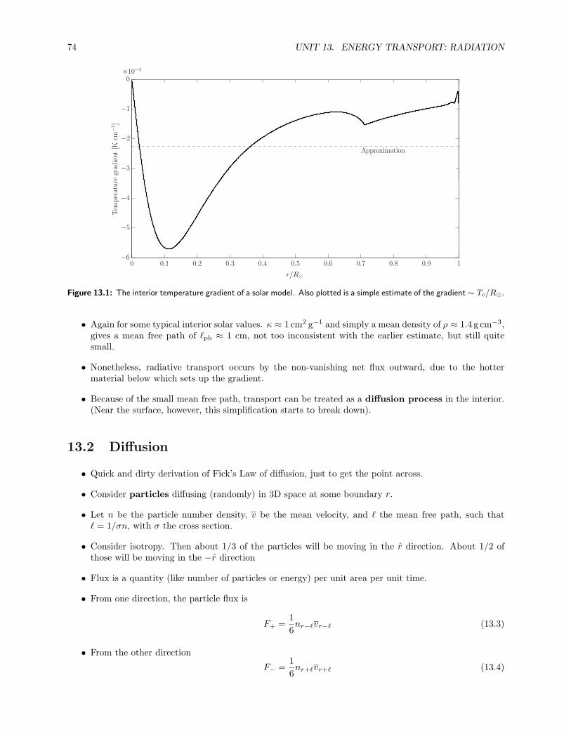
74 UNIT 13. ENERGY TRANSPORT: RADIATION
Approximation
Tem
perature
gradient
[Kcm
−1]
r/R⊙
0 0.1 0.2 0.3 0.4 0.5 0.6 0.7 0.8 0.9 1
×10−4
−6
−5
−4
−3
−2
−1
0
Figure 13.1: The interior temperature gradient of a solar model. Also plotted is a simple estimate of the gradient ∼ Tc/R⊙.
• Again for some typical interior solar values. κ ≈ 1 cm2 g−1 and simply a mean density of ρ ≈ 1.4 g cm−3,gives a mean free path of ℓph ≈ 1 cm, not too inconsistent with the earlier estimate, but still quitesmall.
• Nonetheless, radiative transport occurs by the non-vanishing net flux outward, due to the hottermaterial below which sets up the gradient.
• Because of the small mean free path, transport can be treated as a diffusion process in the interior.(Near the surface, however, this simplification starts to break down).
13.2 Diffusion
• Quick and dirty derivation of Fick’s Law of diffusion, just to get the point across.
• Consider particles diffusing (randomly) in 3D space at some boundary r.
• Let n be the particle number density, v be the mean velocity, and ℓ the mean free path, such thatℓ = 1/σn, with σ the cross section.
• Consider isotropy. Then about 1/3 of the particles will be moving in the r direction. About 1/2 ofthose will be moving in the −r direction
• Flux is a quantity (like number of particles or energy) per unit area per unit time.
• From one direction, the particle flux is
F+ =1
6nr−ℓvr−ℓ (13.3)
• From the other direction
F− =1
6nr+ℓvr+ℓ (13.4)
13.3. FREQUENCY DEPENDENCE OF RADIATION 75
• Net flux
F = F+ − F− =1
6v(nr−ℓ − nr+ℓ), (13.5)
assuming that vr−ℓ ≈ vr+ℓ = v.
• If the mean free path does not change on the scale of the density gradient, then
F =1
6v [nr−ℓ − nr − (nr+ℓ − nr)]
=1
6v
[
−ℓdndr− ℓ
dn
dr
]
F = −D∇rn,
where the diffusion coefficient D = 1/3 v ℓ. This is Fick’s Law. Again, if ℓ is large, this fails.
• This is generic. On the left you have a flux (in this case of number of particles) and on the right agradient of density (in this case number density of particles). Note that the flux is carried from a highconcentration to a low concentration of particles.
• But we want to compute the flux of diffusing radiative energy. So we need an energy density.
• For photons, we can just let v = c, ℓ = ℓph = 1/κρ, and n = u. See Equation (8.3) and note thatu = 3P for a relativistic system, as derived previously, which gives
u = aT 4. (13.6)
• So then the radiative flux Frad is
Frad = −4ac
3
T 3
κρ
dT
dr. (13.7)
• The local luminosity at any point passing through a sphere of radius r is L(r) = 4πr2Frad, so thenrearranging we have
dT
dr= − 3
16πac
κρ
r2L
T 3. (13.8)
• This is a fundamental equation of stellar structure.
13.3 Frequency dependence of radiation
• What we just did was too simple, even in the diffusion approximation. Our answer is in fact integratedover all photon energies.
• In principle, there is a frequency dependence on the flux Fν since the energy density and the opacityare partitioned in frequency.
• Let us go back to Equation (13.6) and instead consider
uν =4π
cBν(T ), (13.9)
where B is the Planck function for a blackbody radiator
Bν(T ) =2hν3
c21
ehν/kBT − 1. (13.10)
This is just from our Bose-Einstein distribution function, Equation (8.1), written in terms of frequencyinstead of momentum.
76 UNIT 13. ENERGY TRANSPORT: RADIATION
• Also keep in mind that the integrated Planck function
B(T ) =
∫ ∞
0
Bν(T ) dν =ac
4πT 4. (13.11)
• Fick’s Law now becomes
Fν = −4π
3
1
κνρ
dBν
dr= −4π
3
1
κνρ
dBν
dT
dT
dr. (13.12)
• The total flux integrated over all frequencies is then
Frad =
∫
Fν dν = −4π
3
1
ρ
dT
dr
∫ ∞
0
1
κν
dBν
dTdν. (13.13)
• Comparing Equation (13.13) with Equation (13.7), we see that the κ in the latter is
1
κ=
π
ac
1
T 3
∫ ∞
0
1
κν
dBν
dTdν. (13.14)
• But since∫ ∞
0
dBν
dTdν =
d
dT
∫ ∞
0
Bνdν =dB
dT=
ac
πT 3, (13.15)
where B = acT 4/4π (the integral over all frequencies), we can then define
1
κR≡ 1
κ=
(∫ ∞
0
1
κν
dBν
dTdν
)(∫ ∞
0
dBν
dTdν
)−1
, (13.16)
where κR is the Rosseland mean opacity.
• All this implies is that Equations (13.7) and (13.8) should replace the opacity by the Rosseland meanopacity:
Frad = −4ac
3
T 3
κRρ
dT
dr, (13.17)
dT
dr= − 3
16πac
κRρ
r2L
T 3. (13.18)
• Note that this weighted opacity gives high frequencies more weight than lower ones (as one could findby differentiating).
• Before we go onto using these expressions to understand stellar structure, let’s look at a few of themajor sources of κR.
Unit 14
Opacity sources
14.1 Kramer’s Laws
• The opacity κ determines how the flux is transported by radiation, and so is an important quantity.
• Computing opacities is hard stuff, only a few groups in the world have succeeded (LANL, LLNL).These computations require full quantum-mechanical treatments.
• In general, opacities can be approximated as power laws of the form
κ = κ0ρnT−s [cm2 g−1], (14.1)
similar to how we treated energy generation rate and its dependence on these parameters.
• The goal is to compute total Rosseland mean opacities from all possible sources, including the followingfour:
1. Scattering of photons from electrons
• Photons, or electromagnetic radiation, can cause free electrons to oscillate at the same frequencyif the energy is low enough. These electrons then radiate this energy. This is a scattering process.
• For relativistic free electrons, this is known as Compton scattering, but for conditions inside moststars, this is Thomspon scattering.
• For temperatures below about 1 billion Kelvin (thermal energies below electron rest mass energy),the cross section for scattering off electrons is frequency independent.
• One finds for the opacity
κe =neσe
ρcm2 g−1, (14.2)
where the cross section is given in the Thompson scattering prescription
σe =8π
3
(
e2
mec2
)2
= 0.6652× 10⁻²⁴ cm2. (14.3)
(Note the classical electron radius buried in there).
• Scattering off electrons will only occur in a highly ionized gas where a sufficient number of electronsare present. Looking back at Equation (5.14) and considering a gas with inconsequential metalsgives
κe ≃ 0.2(1 +X). (14.4)
77
78 UNIT 14. OPACITY SOURCES
• If there are many metals or ionization is incomplete then the electron densities have to be computedmore carefully.
• Below 10,000 K hydrogen is not ionized at low pressure and so this opacity does not contributeto the Rosseland mean.
• For this case, the exponents n = s = 0.
EXAMPLE PROBLEM 14.1: Derive Equation (14.4) in the full ionization case.
2. Free-free absorption
• A single free electron cannot absorb a photon while still conserving energy and momentum.
• If an ion is nearby, this absorption is possible however.
• In this case, it can be shown that the opacity
κf−f ≈ 1023Z2c
µeµIρT−3.5, (14.5)
where Zc is some average nuclear charge. Typically a quantum-mechanical gaunt factor needs tobe included in the coefficient.
• Opacities of this form that scale as κ ∼ ρ T−3.5, or n = 1 and s = 3.5, are known as Kramersopacities.
• The inverse of this process, when an ion changes the momentum of an electron which then emitsa photon, is known as Bremsstrahlung emission
• Note that for reference, in the core of the Sun the product ρT−3.5 ≈ 5× 10⁻²³. So these opacitiesare of order 1 to 10 or so.
3. Bound-free absorption
• Here an ion absorbs a photon which frees a bound electron.
• Causes continuum opacity at wavelengths bluer than the ionizing photon.
• It can be shown that the opacity
κb−f ≈ 1025Z(1 +X)ρ T−3.5. (14.6)
This also has a Kramers form.
• At temperatures below about 104K, this should be used with caution since photons are notenergetic enough to ionize a gas.
• This source of opacity can be larger than free-free absorption by a few orders of magnitude.
4. Bound-bound absorption
• This is photon-induced transitions of electrons between bound levels in an atom or an ion.
• At large temperatures, most photons are ionizing so this contribution is smaller to the totalopacity (maybe 10%).
• Very difficult computations since there are millions of absorption lines possible. Need oscillatorstrengths as well as equation of state.
5. H−
• We just note that in stellar atmospheres (like our Sun) contributions from negative hydrogen andmolecules and grains dominate the opacity.
• Low energy photons starting in the infrared can be absorbed in this bound-free transition.

14.2. CONSEQUENCES 79
Figure 14.1: Opacity contributions in the ρ − T plane. The values are given in units of electron scattering opacity κe.Conduction is not a radiative opacity, and will be discussed in Sec. A.2. From Clayton [1983] after Hayashi et al. [1962].
• What is needed for the H− opacity are free electrons, which at low temperatures might not becompletely abundant from ionization of H.
• Other sources of these electrons are the outer ones from metals, so this is sensitive to metallicity.
• An approximate relation in the range of about 3000-6000K and low densities is
κH− ≈ 2.5× 10⁻³¹
(
Z
0.02
)
ρ1/2T 9 (14.7)
14.2 Consequences
• Figure 14.1 shows the contributions from different opacity sources in a stellar interior.
• At low temperatures and partial ionization, b-b and b-f absorption dominates from the bound electrons.
• As ionization occurs at higher temperatures, free-free opacity takes over, but as T continues to increase,κf−f decreases and scattering from free electrons dominates.
• In reality, all of these processes are occuring at any one time and place, so contributions must be addedcorrectly.
• Note that the sum of the Rosseland mean opacities of each component is not the same as the Rosselandmean of the sum
• Figure 14.2 shows opacity data from the OPAL project.1 We see that the Sun’s opacity can reach 105
or so near the surface where atoms recombine.1http://opalopacity.llnl.gov/
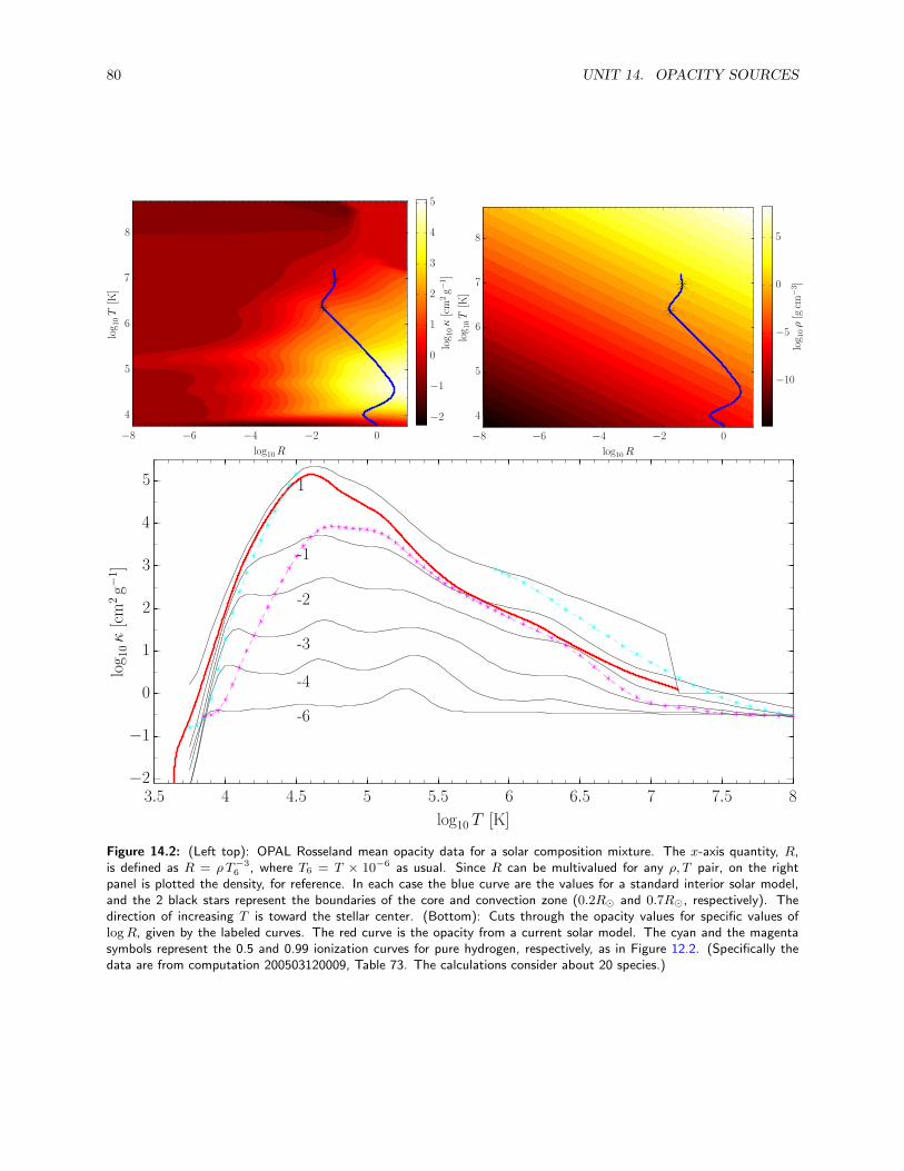
80 UNIT 14. OPACITY SOURCES
log 1
0κ[cm
2g−
1]
log 1
0T
[K]
log10R
−8 −6 −4 −2 0
−2
−1
0
1
2
3
4
5
4
5
6
7
8
log 1
0ρ[gcm
−3]
log 1
0T
[K]
log10R
−8 −6 −4 −2 0
−10
−5
0
5
4
5
6
7
8
log 1
0κ[cm
2g−
1]
log10 T [K]
1
-1
-2
-3
-4
-6
3.5 4 4.5 5 5.5 6 6.5 7 7.5 8−2
−1
0
1
2
3
4
5
Figure 14.2: (Left top): OPAL Rosseland mean opacity data for a solar composition mixture. The x-axis quantity, R,is defined as R = ρ T−3
6 , where T6 = T × 10−6 as usual. Since R can be multivalued for any ρ, T pair, on the rightpanel is plotted the density, for reference. In each case the blue curve are the values for a standard interior solar model,and the 2 black stars represent the boundaries of the core and convection zone (0.2R⊙ and 0.7R⊙, respectively). Thedirection of increasing T is toward the stellar center. (Bottom): Cuts through the opacity values for specific values oflogR, given by the labeled curves. The red curve is the opacity from a current solar model. The cyan and the magentasymbols represent the 0.5 and 0.99 ionization curves for pure hydrogen, respectively, as in Figure 12.2. (Specifically thedata are from computation 200503120009, Table 73. The calculations consider about 20 species.)

14.2. CONSEQUENCES 81
Wavelength[angstrom
]
log10 T [K]
4 4.5 5 5.5 6
1000
2000
3000
4000
5000
6000
Figure 14.3: Blackbody curves for a range of wavelengths and temperatures. The curve at each temperature is normalizedto its maximum value across wavelengths. Wavelength guides from top to bottom are at 1216 A, 912 A, and 228 A.
• Figure 14.2 can be understood in a few limiting cases:
– For the low density, high temperature case (small R), and for the high temperature regime at anydensity, all H and He is ionized and the electrons are free particles. Here we expect electron scat-tering, where Equation (14.4) is dominant. Indeed, κe ≈ 0.34 cm2 g−1 for an X = 0.7 composition,which agrees with the values over most of the temperature range (log10−0.34 ≈ −0.47).
– Below 10,000 K the opacities all converge to small values. Here, all electrons go to the groundstate of H and He. Incoming photons can only cause a bound free transition if their wavelengthsare shorter than 912 A (for H) or 228 A (for HeII). In fact, the whole Lyman series (edge) onlyextends to 1216 A (for H). But at this temperature, the blackbody curve is peaked at about2880 A, and there just aren’t many photons with such high energies available. The stellar regionin which this applies is near the surface, but the Sun does not have such conditions as the plotsshow. Also see Figure 14.3.
– At intermediate temperatures we see increased opacity, particularly as the density increases (largerR). Even for the lowest density curve we see a bump around temperatures of 5.0-5.5. Wien’s lawtells us the wavelengths are in the 100 − 300 A range. This suggests the HeII Lyman edge, eventhough there aren’t many He ions. The bump at about 4.5-4.75 at larger densities could be dueto a bound-free absorption of HeI. In any case, these large radiative opacities are found in the Hand He ionization zones in stars.
– Note the Kramers shape to the opacities, which decrease at higher temperatures.
– Keep in mind however that these are mean opacities, independent of individual wavelengths.

82 UNIT 14. OPACITY SOURCES
Unit 15
Convection
Another important carrier of energy from the stellar interior outward is convection.
15.1 Temperature gradients (“dels”)
• There are several manipulations we can carry out to make the expressions we derived more useful forlater.
• For future use we will need different forms of Equation (13.8). Take hyrdrostatic equilibrium and uselogarithmic derivatives:
d lnP
d ln r= −Gmρ
rP. (15.1)
• Dividing both sides by d lnT/d ln r gives a new quantity we’ll call “del”
∇ ≡ d lnT
d lnP= − r2P
Gmρ
1
T
dT
dr, (15.2)
which is the true driving gradient in the star.
• If we now consider that the luminosity L is carried ONLY by radiation, then we can define “delrad”
∇rad ≡(
d lnT
d lnP
)
rad
=3
16πacG
PκR
T 4
L
m, (15.3)
where we used Equation (13.8).
• So if ∇ = ∇rad, then all the luminosity is radiative. If ∇rad > ∇, there is some other transportmechanism of the energy in addition to radiation.
• This quantity is the local slope which is required if all the luminosity were carried by radiation throughdiffusion.
• In fact, we will use this as a comparison in this unit to a similar quantity we’ve already introduced inEquation (11.14),
∇ad ≡(
d lnT
d lnP
)
ad
=Γ2 − 1
Γ2. (15.4)
where this is defined in an “adiabatic” sense, or, i.e., at constant entropy.
• The value of 0.4 comes when considering an ideal gas:
∇ad =53 − 1
53
=2
5= 0.4. (15.5)
This is an important number to keep in mind.
83
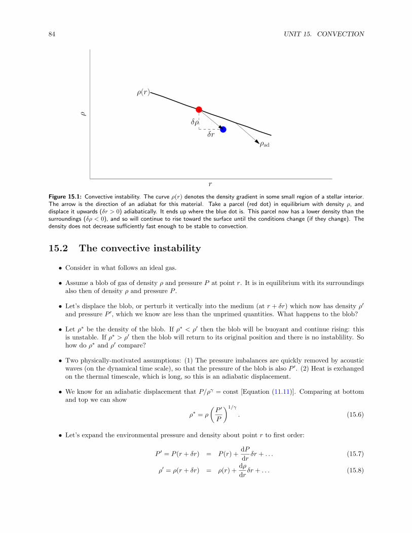
84 UNIT 15. CONVECTION
ρ
r
ρad
ρ(r)
δr
δρ
Figure 15.1: Convective instability. The curve ρ(r) denotes the density gradient in some small region of a stellar interior.The arrow is the direction of an adiabat for this material. Take a parcel (red dot) in equilibrium with density ρ, anddisplace it upwards (δr > 0) adiabatically. It ends up where the blue dot is. This parcel now has a lower density than thesurroundings (δρ < 0), and so will continue to rise toward the surface until the conditions change (if they change). Thedensity does not decrease sufficiently fast enough to be stable to convection.
15.2 The convective instability
• Consider in what follows an ideal gas.
• Assume a blob of gas of density ρ and pressure P at point r. It is in equilibrium with its surroundingsalso then of density ρ and pressure P .
• Let’s displace the blob, or perturb it vertically into the medium (at r + δr) which now has density ρ′
and pressure P ′, which we know are less than the unprimed quantities. What happens to the blob?
• Let ρ∗ be the density of the blob. If ρ∗ < ρ′ then the blob will be buoyant and continue rising: thisis unstable. If ρ∗ > ρ′ then the blob will return to its original position and there is no instablility. Sohow do ρ∗ and ρ′ compare?
• Two physically-motivated assumptions: (1) The pressure imbalances are quickly removed by acousticwaves (on the dynamical time scale), so that the pressure of the blob is also P ′. (2) Heat is exchangedon the thermal timescale, which is long, so this is an adiabatic displacement.
• We know for an adiabatic displacement that P/ργ = const [Equation (11.11)]. Comparing at bottomand top we can show
ρ∗ = ρ
(
P ′
P
)1/γ
. (15.6)
• Let’s expand the environmental pressure and density about point r to first order:
P ′ = P (r + δr) = P (r) +dP
drδr + . . . (15.7)
ρ′ = ρ(r + δr) = ρ(r) +dρ
drδr + . . . (15.8)

15.2. THE CONVECTIVE INSTABILITY 85
• Substitute Equations (15.7)-(15.8) into (15.6) and expand (binomial):
ρ∗ = ρ+ρ
γP
dP
drδr. (15.9)
• For an instability to occur, ρ∗ − ρ′ < 0, or
ρ∗ − ρ′ =ρ
γP
dP
drδr − dρ
drδr < 0. (15.10)
• So, an instability occurs if
(
dρ
dr
)
ad
<dρ
dr, (15.11)
where we introduced the adiabatic gradient
(
dρ
dr
)
ad
=1
Γ
ρ
P
dP
dr, (15.12)
where we’ve denoted γ = Γ in the adiabatic case.
• This can be interpreted as the density gradient resulting from adiabatic motion in the given pressuregradient.
• Since the gradient of pressure is always negative (hydrostatic equilibrium), instability occurs when thedensity does not decrease sufficiently rapidly compared to the adiabatic case.
• See Figure 15.1 for a schematic of this.
• Note that it is convention to express Equation (15.11) as
d ln ρ
d lnP<
1
Γ1. (15.13)
(Note since we’ve divided by a negative number, d lnP/dr, the inequality changes). For a fully ionizedideal gas, the RHS is 3/5.
• Let’s now consider the force per unit volume acting on the displaced blob. That force (buoyancy andgravitational) is F = −(ρ∗ − ρ′)g, since g acts downwards.

86 UNIT 15. CONVECTION
IN CLASS WORK
Use this force in Newton’s second law and derive a simple equation of motion for the displace-ment δr. Show that a characterstic frequency N comes out
N2 =g
ρ∗
(
ρ
γP
dP
dr− dρ
dr
)
=g
ρ∗
[(
dρ
dr
)
ad
− dρ
dr
]
, (15.14)
called the Brunt-Vaisala frequency. Examine the solutions of the equation of motion based onthe possible values of N in the stable or unstable condition.
Answer:From Newton’s second law
ρ∗d2δr
dt2= −(ρ∗ − ρ′)g.
If we plug in Equation (15.10) we get the equation of motion
d2δr
dt2+N2δr = 0,
where N is the Brunt-Vaisala frequency given above.A general solution to this equation is δr ∝ e±iNt.If the medium is stable to convection, we know that N2 > 0. When this is the case, the solution isthus sinusoidal and the blob δr oscillates about a given point (gravity/buoyancy waves).In the other case, N2 < 0 and so N is imaginary: N → iN . The the solution goes as δr ∝e−Nt + eNt. This solution describes an exponentially growing parcel, in other words, a convectiveinstability.
Unit 16
Convection 2
16.1 Other formulations of the instability
• It is convenient to look at the stability criterion in terms of temperature gradients instead.
• Using Eq. (15.8) and the ideal gas law P = ρRT/µ (ignore gradients in mean molecular weights FORNOW) we can show that
ρ′ = ρ+ρ
p
dP
drδr − ρ
T
dT
drδr. (16.1)
• For instability, again, we then require that δρ < 0, or
ρ∗ − ρ′ =
(
1
γ− 1
)
ρ
P
dP
drδr +
ρ
T
dT
drδr < 0. (16.2)
• Now the instability condition becomes(
dT
dr
)
ad
>dT
dr, (16.3)
where the adiabatic temperature gradient is given by(
dT
dr
)
ad
=
(
1− 1
γ
)
T
P
dP
dr. (16.4)
• This says that if the temperature gradient decreases too steeply out through the star there will beconvection.
• To simplify in analogy with what we did before (Eq. 15.13), it is convention to write the inequality as
d lnT
d lnP>
Γ2 − 1
Γ2. (16.5)
• We reintroduce
∇ =d lnT
d lnP, ∇ad =
Γ2 − 1
Γ2, (16.6)
so that the instability condition is∇ > ∇ad. (16.7)
Again, the RHS is 2/5 in the ionized ideal case.
• This is known as the Schwarzschild criterion. The inequality is also referred to as superadiabaticity.
87
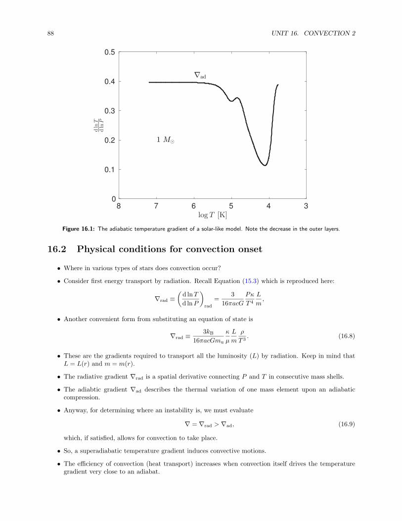
88 UNIT 16. CONVECTION 2
345678
log T [K]
0
0.1
0.2
0.3
0.4
0.5
dlnT
dlnP
1 M⊙
∇ad
Figure 16.1: The adiabatic temperature gradient of a solar-like model. Note the decrease in the outer layers.
16.2 Physical conditions for convection onset
• Where in various types of stars does convection occur?
• Consider first energy transport by radiation. Recall Equation (15.3) which is reproduced here:
∇rad ≡(
d lnT
d lnP
)
rad
=3
16πacG
Pκ
T 4
L
m,
• Another convenient form from substituting an equation of state is
∇rad ≡3kB
16πacGmu
κ
µ
L
m
ρ
T 3. (16.8)
• These are the gradients required to transport all the luminosity (L) by radiation. Keep in mind thatL = L(r) and m = m(r).
• The radiative gradient ∇rad is a spatial derivative connecting P and T in consecutive mass shells.
• The adiabtic gradient ∇ad describes the thermal variation of one mass element upon an adiabaticcompression.
• Anyway, for determining where an instability is, we must evaluate
∇ = ∇rad > ∇ad, (16.9)
which, if satisfied, allows for convection to take place.
• So, a superadiabatic temperature gradient induces convective motions.
• The efficiency of convection (heat transport) increases when convection itself drives the temperaturegradient very close to an adiabat.
16.3. DEPTH OF OUTER CONVECTION ZONES 89
• Let that sink in: Once convection is set up, it tends to drive ∇ very close to ∇ad. So it goes fromsuperadiabatic to nearly adiabatic.
• Examining the condition in Eq. (16.9), we see that convection may occur if
– L/m is large. Think of this as L/m ∼ dL/dm = ε at small m (near the core). The energygeneration rate is huge in massive stars in the cores, so many massive stars have convective cores.
– κ is large. This is satisfied in the outer parts of less-massive stars, or with low surface temperaturesand ionization zones of hydrogen (Sun).
– ρ/T 3 is large. Happens typically in the outer parts of relatively cool stars. In fact, this ratioincreases rapidly as the effective temperatures go down.
– ∇ad = 1 − 1/γ is small. Satisfied in the ionization zone of hydrogen, in outer parts of cool starswhere γ gets small (increased specific heat). See Figure 16.1.
• n = 1.5 polytropes are good models for convective regions, as this corresponds to γ = 5/3.
16.3 Depth of outer convection zones
• We’ve seen where convection tends to set in, but how large are these regions and what do they dependon?
• To first order the depth depends on Teff , since this determines where ionization layers are.
• Stars with lower surface temperatures achieve H ionzization at deeper depths with higher pressure.
• So for cool main-sequence stars, outer convection zones can extend deep, even to the center.
• For hotter stars, up to about 8000K, ionization occurs higher and higher in the atmosphere, and theconvective shells of these stars can be very thin.
• The depth can also depend on chemical abundances.
• Consider a star with relatively high He abundance.
• The larger mean molecular weight corresponds to lower pressures at a given layer.
• He ionization, which can cause a convective instability, thus happens at a deeper layer, or highertemperature.
• Convection zones will be deeper for He-rich stars.
• For metal-poor stars, the opacity is reduced and therefore the radiative temperature gradient getsreduced, reducing the convective instability.
• Metal-poor stars will have shallower convection zones than metal-rich ones.
16.4 Semiconvection
• Let’s return to the Brunt-Vaisala frequency again from Equation (15.14):
N2 = g
(
1
γP
dP
dr− 1
ρ
dρ
dr
)
.
90 UNIT 16. CONVECTION 2
• We want to rewrite this in a very convenient form, and this time we will take into account compositiongradients in the gas to be as general as possible. The form is
N2 =g2ρ
P(∇ad −∇+∇µ), (16.10)
where (as some have been defined before)
∇ =d lnT
d lnP, ∇ad =
(
d lnT
d lnP
)
ad
, ∇µ =d lnµ
d lnP. (16.11)
EXAMPLE PROBLEM 16.1: Show how you can get from Equation (15.14) to Equation (16.10). Startwith
N2 = g
(
1
γ
d lnP
dr−
d ln ρ
dr
)
,
P =ρT
µ,
d lnP = d ln ρ+ d lnT − d lnµ.
Answer:
N2 = g
(
1
γ
d lnP
dr−
d ln ρ
dr
)
,
P =ρT
µ,
d lnP = d ln ρ+ d lnT − d lnµ,
N2 = g
(
1
γ
d lnP
dr−
d lnP
dr+
d lnT
dr−
d lnµ
dr
)
,
= g
(
d lnP
dr
(
1− γ
γ
)
+d lnT
dr−
d lnµ
dr
)
,
= g
(
−∇ad
d lnP
dr+
d lnT
dr−
d lnµ
dr
)
,
= gd lnP
dr
(
−∇ad +d lnT
dr
dr
d lnP−
d lnµ
dr
dr
d lnP
)
,
= gd lnP
dr(−∇ad +∇−∇µ) ,
=g
P
dP
dr(−∇ad +∇−∇µ) ,
= −g2ρ
P(−∇ad +∇−∇µ) ,
N2 =g2ρ
P(∇ad −∇+∇µ) .
• Ignore the composition gradient for a second. We recover the “standard” stability relation: if the tem-perature gradient is larger than the adiabatic one (Schwarzchild), the BV frequency becomes complex.
• If it’s the reverse, the BV is positive and the medium is stable to convection.
• Now however, we have the possibility that the Schwarzchild criterion is satisfied (∇ > ∇ad), yet themedium remains stable because the composition gradient makes it positive again.

16.5. MIXING LENGTH THEORY 91
• This is the Ledoux criterion, and when this is the case we have weak convection, or semiconvection.
• This typically would not occur in a convection zone, why? Because convection mixes material andcomposition gradients are removed.
• But in areas of nuclear burning where gradients do exist, and at the “edges” of convection zones, thissituation can arise. Large peaks in the µ-gradient (also caused by g increases) can cause large jumpsin N .
• Can be thought of as difficulty in moving “heavier” material (high µ) up - it doesn’t want to do that.
• Becomes important for red-giant stars and their gravity modes mixing (boosting frequency) with acous-tic modes.
16.5 Mixing length theory
• How does the convection actually transfer the energy?
• We have previously shown how convection can take place by considering a blob displaced from itsequilibrium position.
• The blob is hotter than its surroundings.
• This blob rises with a velocity up to a point where a new hydrodynamic instability sets in, wherebythe motion becomes turbulent and the blob dissolves, depositing its heat in the surroundings.
• The exact details of this process are still unknown and are a subject of much research. For solarconvection, the most sophisticated numerical simulations carried out on the fastest computers take anorder of magnitude more computation time than the solar “time” they are trying to simulate, and thatis just for a small section of the Sun.
• In comparison, computing the solar model over the Sun’s lifetime, with a simple model of convection,takes a couple minutes.
• Remember that the radiative flux L/4πr2 is
Frad =4ac
3
T 3
κρ
dT
dr=
4acG
3
mT 4
κPr2∇,
using hydrostatic equilibrium. ∇ is the actual stratification.
• Neither Frad or ∇ are really known, since radiation only carries some of the star’s flux.
• But we did note that the temperature gradient required to carry all of the stellar luminosity is ∇rad.If this includes convection, the total flux then is
Ftot = Frad + Fconv =4acG
3
mT 4
κPr2∇rad. (16.12)
• A very reasonable convective flux for a parcel in pressure equilibrium is its heat content multiplied bythe mass flux:
Fconv = ρvcP∆T. (16.13)
• All that’s left to do is find ρ, v and ∆T of the blob.
• ∆T = Ti − T is the excess heat of a rising parcel of gas with respect to its surroundings.
92 UNIT 16. CONVECTION 2
• Assume a parcel moves a distance ℓ before dissolving into the background material, so that at anygiven time, a typical parcel will have moved ℓ/2. The temperature difference between the parcel andthe gas is
∆T = Ti − T =
(
dTi
dr− dT
dr
)
ℓ
2. (16.14)
• Multiply by the pressure scale height HP = − (d lnP/dr)−1
and divide by T
∆T
T= (∇−∇i)
ℓ
2HP. (16.15)
• If the parcel remains in pressure equilibrium, assuming a general equation of state, then changes in itsdensity are
dρ
ρ= −δdT
T= −δ(∇−∇i)
ℓ
2Hp, (16.16)
where
δ = − d ln ρ
d lnT. (16.17)
• Since the density difference implies a buoyancy force −g(ρi − ρ), there is work that goes into movingthe parcel
− g(ρi − ρ)ℓ
2= gρδ(∇−∇i)
ℓ2
4Hp. (16.18)
• Suppose half of the work goes into the kinetic energy of the parcel, and the other half goes into thesurroundings, moving it aside. The velocity is then
v2 =ℓ2
4
gδ(∇−∇i)
Hp. (16.19)
• We get for the convective flux then that
Fconv = ρcpT (gδ)1/2 ℓ
2
4H−3/2
p (∇−∇i)3/2. (16.20)
• It is possible to compute ∇i, because as the parcel moves its internal energy will change because ofradiative losses and adiabatic expansion/contraction. One finds
∇i −∇ad
∇−∇i=
6acT 3
κρ2cpvℓ. (16.21)
• The overal problem can now be solved. Five new equations for the 5 unknowns Frad, Fconv, v, ∇, and∇i. The mixing-length parameter α = ℓ/HP is used as a free parameter, chosen to match observations.
• Solutions can be found in the literature. Limiting cases are interesting. In dense regions of a star,∇ → ∇ad. A gradient just over the adiabatic limit is all that is necessary to transport all of theluminosity.
• Near stellar photospheres, ∇ → ∇rad, and convection is ineffective so F → Frad.
• In between these limits, the mixing-length equations need to be solved.
• Near the surface, convection does not transport energy efficiently, since convective flux is proportionalto the the density which is quite low.
• It is also proportional to the mixing length which has to be small. So the only way for convection todominate is if δ can get large. This means it has to be very far from adiabatic.
16.6. CONVECTIVE OVERSHOOT 93
• We know this because we see granulation, which typifies the size of convective elements, about 10−3R⊙.
• The convective time scale
tconv ≃[(
d lnT
d ln r
)
ad
− d lnT
d ln r
]−1/2
tdyn. (16.22)
• This timescale is a dynamical time scale, but since the gravitational acceleration is reduced because ofthe difference in density that comes into all of this, the timescale is increased by that pre-factor.
• That prefactor in the Sun is of order 10−6, and we find convective time scales tconv ≃ 0.2 yr.
• This is still small compared to evolution. Matter mixes over such a time scale in the convection zone.
16.6 Convective overshoot
• We briefy mention this here because it has very important implications for stellar modeling.
• The parcels we consider unstable to convection will eventually reach a stable layer.
• However the momentum causes them to overshoot the boundary into this stable layer.
• For example, this is why we see granulation in the solar photosphere (which is stable).
• One important consequence of this overshoot is the deposition of convectively mixed material intostable regions, which can affect the thermal structure as well as evolutionary properties.
16.7 An entropy formulation
• Convection can also be understood in terms of entropy.
• For reversible processes, dQ = TdS and so
T dS = dU + PdV. (16.23)
• Using standard thermodynamic relations, it can be shown from here that
dS
dr= cP (∇−∇ad)
d lnP
dr. (16.24)
• So if the star is radiative, dS/dr > 0 and the entropy increases outward.
• If the star is convective, dS/dr < 0. If the convection is efficient the gradient is very close to beingadiabatic, meaning the entropy is very nearly constant throughout convection zones.
16.8 An energy formulation
• Start with Equation (16.4) and rewrite using ideal gas law and hydrostatic equilibrium:
(
dT
dr
)
ad
=
(
1− 1
γ
)
µ
ρRg
dP
dr= −
(
1− 1
γ
)
gµ
Rg. (16.25)
94 UNIT 16. CONVECTION 2
• Remembering that γ = cP /cV and cP − cV = Rg/µ,
(
dT
dr
)
ad
= −(
cP /cV − 1
cP /cV
)
gµ
Rg, (16.26)
= −(
cP−cVcV
cP /cV
)
gµ
Rg, (16.27)
= −(
cP − cVcP
)
gµ
Rg, (16.28)
(
dT
dr
)
ad
= − g
cP. (16.29)
• This form shows how the parcel of gas is changing as it rises adiabatically and expands
• This can also be derived using energy by considering energy release and work against gravity
• To see this, consider again a parcel of gas at position r that is displaced adiabatically to r + dr. Thetemperature at the new depth is T + dT .
• The temperature gradient dT/dr will be negative in our case since T decreases as we move furtherfrom the center. So when the parcel arrives at the new location, it is in cooler surroundings, so theparcel has more internal energy than the local gas.
• If we let time elapse a bit and the parcel releases energy to the surroundings, the amount of thermalenergy released at fixed pressure is Cp dT erg g−1. Is this energy release important?
• The other factor at work here is gravity, and we have to ask if the work done against gravity to movethe parcel upwards balances the release of thermal energy.
• The work done against gravity is g dr per gram of material. Therefore, the total amount of energy todisplace 1 gram of material is
∆E = g dr + Cp dT. (16.30)
Note that the sign can be either positive or negative (since dT will usually be negative). Let’s say thatthe gravitational energy exceeds the thermal energy released, so that the change in energy is positive.In this case, it has taken more work to displace the gas than what is released as thermal energy, andso the final energy state is higher. Therefore, the parcel will sink down to its initial position in a lowenergy state. There is no reason for it to move. Is is convectively stable.
In the opposite case, the release of thermal energy is more than enough to compensate for the workagainst gravity. There will even be some excess, and the parcel will still be hotter than its surroundings.It may continue on rising. This is a convective instability, as we have already studied.
• So, the boundary between the two cases is when g dr = −Cp dT , which occurs when the temperaturegradient takes on a particular value of the adiabatic temperature gradient
dT
dr
∣
∣
∣
ad= − g
Cp. (16.31)
For convection to occur, dT/dr < dT/dr|ad. Since both gradients are negative, this can also be writtenfor instability
∇ > ∇ad. (16.32)
This is the same conclusion we reached earlier.
16.8. AN ENERGY FORMULATION 95
COMPUTER PROBLEM 16.1: [80 pts]: This assignment deals with convection and radiation zones inmain-sequence stars over a range of different masses. You are going to quantitatively illustrate where weexpect such zones to exist in stars to provide an overall understanding of stellar structure during the periodof core-hydrogen burning.
What to do
Your overall goal is to prepare a main plot (described in more detail below) showing where these zones exist.For this purpose, you need to run a bunch of MESA models for different mass stars. We will use these modelsfor future studies so make sure to keep the directory(ies) neat and handy.
1. The models should be within the stellar mass range of M∗ = 0.3M⊙ − 20M⊙. The number of modelsyou compute is up to you, but the “mass grid” should be sufficiently populated so you don’t missany important details, and so that you can make the required plots with enough number of pointsand precision. Somewhere between 10 and 20 models seems reasonable. One of the models should beM∗ = 1M⊙, of course!
2. The models are to be of solar hydrogen mass fraction and metallicity (Z = 0.02). For each mass, youwill run the code until the core looks like the core of today’s Sun, X ≈ 0.35, which is the model youwill want to use for what follows. You will also want the history data (really just Teff and L) for theZAMS (zero-age main sequence) point, where X ≈ 0.7. You shouldn’t need to run pre-main sequencemodels.
3. That’s all you need to do with MESA. Now you need to carefully explore the resulting data and determinethe locations of all the convection and radiation zones for each star mass. Use the criteria discussed inclass.
What to hand in
After reading the below information you will find you need to hand in at least 7 plots, as well as text pertainingto items 4 and 6.
1. A nice H-R diagram of your stars. The symbol size should represent the star’s radius, and the color thestar’s mass at the time you stopped your models. Also give an indication of age somehow discretelyso we have an idea of the range there. Finally, plot a small symbol for where each star began on theZAMS, so we see how much “evolution” occured. These symbols do NOT need to show the mass orradius information as in the more evolved points. [15 pts]
2. A plot that shows where the internal convection and radiation zones are for each star. [25 pts]
• This should be a publication-quality plot (clearly labeled, easy to read, useful for future reference,etc.).
• The plot is to be as follows: the x axis is logM∗/M⊙ and the y axis is m(r)/M∗.
• The interior radiation and convection zones should be clearly demarcated by however you wish todo it.
• Finally, somehow denote the dominant H-burning process for everywhere that nuclear burning istaking place. In many cases, you will have some regions where PP is dominant and some whereCNO is (in the same star).
3. A second plot of exactly the same information but instead where r/R∗ is the ordinate. These shouldbe on separate pieces of paper. [5pts]
4. A summary paragraph or two of how you obtained the parameters in your plot, i.e., how you determinedwhere the zones are from the stellar profiles. Mention here any issues you ran into or anomalous cases(if any). You don’t need to do much interpretation here, just write down what you did to gather theinformation that went into these plots. [10pts]
5. Pick two of your models. One should be M∗ ≤ 1.1M⊙ and one M∗ ≥ 3M⊙. For each of these 2 modelsyou will make 2 more plots, so 4 in total here. One of the plots for each mass should have the threequantities ∇, ∇ad, and ∇rad plotted as a function of interior log T , but reversed, so log T decreasesto the right. The other plot for each mass will be the Brunt-Vaisala frequency (squared), or N2 inappropriate units as a function too of reversed log T . Make sure it’s scaled properly as to be visible.[10pts]
96 UNIT 16. CONVECTION 2
6. Write another page or two on the above 4 plots. Describe what is happening and connect what youobserve in these figures to the findings shown in your main plot. Compare and contrast the behaviorfor the 2 different masses. Try to describe and decipher any unusual “features” you see, such as bumpsor spikes, in each case. Connect them to things we may have discussed in class, not forgetting, forexample, our study of the opacities. Indeed, you may find it necessary to generate other supplementaryplots of other quantities in the models to get your point across here. Feel free to draw on and labelthese plots by hand to point things out. Be thorough. Also in this part, be sure to answer the followingquestion for each of these 2 stellar mass models:
• In the interior regions where ∇rad is large, what is your idea as to the physical reasons causingthis?
Use Equation (16.8) from the notes as a guide if needed. [15 pts]
Things to keep in mind
1. Your main plot is going to be judged by the faculty to determine who made the best publication-qualityimage (oh, and it should be correct too). Therefore the plot should be full page and nice, and on aseparate page from your other stuff! You also may want to keep it secret from your classmates so theydon’t steal your ideas. An emailed .pdf or .eps of your plot would also be good and I can collect themall into one document to show in high quality on a computer screen. The one judged best will receivea special prize extra credit on the assignment.
2. You may want to consider your initial stellar mass grid spaced out regularly in terms of logM∗/M⊙,rather than in linear M∗/M⊙. But do what you want. Much of the changes to convection propertiesoccur in the 1− 2 M⊙ range.
3. You may need to consider adding quantities to what MESA saves in the profiles. This is easily done usingthe .list files. Your best bet might be copy the default profile columns.list file into your working directoryand uncomment the things you’ll need. If you do that, comment out the line in your inlist project thatjust uses the custom profiles.list. Let me know if you need help.
4. You likely don’t need to create any pre-main-sequence models because the metallicity we are using isstandard.
5. It may or may not be reasonable to interpolate certain quantities to make your mass grid denser foryour plots. It’s up to you.
6. There are very fast and easy, or long and complicated ways of obtaining the profile quantities you needfor the plots. Hopefully you find the fast/easy ways.
7. Try to understand what’s going on in each model. This will be helpful for grasping the evolution ofstars of different masses.

Part II
Stellar Evolution
97


Unit 17
Overview of Asteroseismology
• The surface of a star oscillates with displacements in the radial and horizontal directions as:
δr = ξrr + ξh,
• The diplacements are solutions to the equations of motion expressed as
ξr(r, θ, φ, t) =√4π ξr(r)Y
mℓ (θ, φ) exp(−iωt) (17.1)
and
ξh =√4πξh(r)
(
∂Y mℓ
∂θθ +
1
sin θ
∂Y mℓ
∂φφ
)
exp(−iωt). (17.2)
• The r dependence terms are the (as of yet undetermined) eignenfunctions of the star, while ω is theangular eigenfrequency of a mode
• The Y mℓ are spherical harmonics
• Three “quantum” numbers describe each mode: n gives the overtone, or number of nodes in the radialdirection
• ℓ is the degree and specifies the number of surface nodes
• m is the azimuthal order and |m| gives the number of nodal lines of longitude
• The equations of motion are derived from hydrodynamics (continuity, momentum, energy, Poisson,etc.) and approximations to them
• Namely 2: adiabatic small-amplitude (linear) changes
• After the approximations and plugging the spherically symmetric expansions into them, a set of coupleddifferential equations are derived
• These are then solved for the eigenfrequencies and eigenfunctions
• The pulsations can be classified in various ways
• Radial modes are the simplest with ℓ = 0, these are the breathing modes.
• The star expands and contracts, heats and cools. The fundamental mode is what is foundin Cepheidand RR Lyrae stars.
• The center is a node and the surface is an antinode
99
100 UNIT 17. OVERVIEW OF ASTEROSEISMOLOGY
• The first overtone n = 2 has 1 node away from the center.
• The motions above and below that region move in antiphase
• When stars exhibit both fundamental and first overtone pulsations, the ratio of their frequencies canbe used to determine interior properties
• Unlike musical instruments, their ratios vary, which at least tells us that stars do not have constanttemperatures or uniform sound speed
• Nonradial modes have ℓ > 0 and n ≥ 1, thus, a surface node
• These modes are degenerate in m as there are 2ℓ+ 1 modes with the same frequency
• Rotation and possibly other effects can break this degeneracy
• The simplest is the dipole ℓ = 1 mode
• The equator is a node, so the northern hemisphere will expand while the southern contracts, and viceversa
• Depending on n there are internal radial nodes as well
• ℓ = 2 are quadrupolar, while ℓ = 3 are octupolar modes
• Beyond this, except for the Sun, we cannot detect higher-degree modes, as the surface averagingpartially cancels neighboring regions of hot/cold (intensity) or up/down (Doppler velocity)
• Nodal regions beyond about ℓ = 3 are practically unattainable in disc-integrated observations (includ-ing for the Sun)

Unit 18
Theory of the Main Sequence
18.1 Summary of stellar structure
• Mass and radius relationshipdm
dr= 4πr2ρ
• Hydrostatic equilibriumdP
dr= −gρ
• EnergydL
dr= 4πr2ρε
• Energy transportL = 4πr2(Frad + Fconv)
– Radiation
Frad = −4acT 3
3κRρ
dT
dr
– Convection
Fconv = ρCpT (gδ)1/2 ℓ
2
4H−3/2
p (∇−∇ad)3/2.
• Equation of state
P =ρkBT
µmu+
a
3T 4
• Rosseland opacityκR = κR(ρ, T, µ)
• Energy generationε = ε(ρ, T, µ) = εnuc + εgrav
whereεnuc = ε0ρT
n, (18.1)
and
εgrav = −T dS
dt
is related to Kelvin-Helmholtz contraction (and note the time dependence).
101

102 UNIT 18. THEORY OF THE MAIN SEQUENCE
• Abundance changes
dX
dt= − εnuc
26.7MeVdY
dt= −dX
dt
• Boundary conditions
r −→ 0; m(r) −→ 0
r −→ 0; L(r) −→ 0
r −→ R; m(r) −→M
r −→ R; ρ(r) −→ 0
r −→ R; T (r) −→ Teff
• Vogt-Russell Theorem
– There are only 2 free parameters in the equations needing to be solved: the total stellar mass Mand the chemical composition.
– The theorem states that just these 2 parameters uniquely determine the structure of any star.Then, evolution is only based on the changing of the composition due to nuclear burning.
18.2 Homology relations for stars in radiative equilibrium
• Solving the equations of stellar structure is possible, yet difficult.
• There are ways of obtaining useful insights without doing so (like using the first 2 equations to studypolytropes).
• This involves basic unit analysis.
• Let’s take a simplified subset of the equations written above and express them in terms of the masscoordinate, rather than position:
dr
dm=
1
4πρr2, (18.2)
dP
dm= − Gm
4πr4, (18.3)
dF
dm= ε0ρT
n, (18.4)
dT
dm= −3 3
4ac
κ
T 3
F
(4πr2)2, (18.5)
P =RgρT
µ. (18.6)
• We’ve neglected things like radiation pressure and taken simple opacities.
• Now introduce the dimensionless mass fraction parameter
x =m
M∗
, (18.7)
so that our functions may be expressed now in terms of dimensionless functions of x:

18.3. DEPENDENCE ON MASS 103
r = f1(x)R∗, (18.8)
P = f2(x)P∗, (18.9)
ρ = f3(x)ρ∗, (18.10)
T = f4(x)T∗, (18.11)
F = f5(x)F∗. (18.12)
• Now, plugging in these scaling equations Eqs. (18.8)-(18.12) into Eqs. (18.2)-(18.6) gives
df2dx
= − x
4πf41
; P∗ =GM2
∗
R4∗
, (18.13)
df1dx
=1
4πf21 f3
; ρ∗ =M∗
R3∗
, (18.14)
f2 = f3f4; T∗ =µP∗
Rgρ∗, (18.15)
df4dx
= − 3f54f3
4 (4πf21 )
2; F∗ =
ac
κ
T 4∗R
4∗
M∗
, (18.16)
df5dx
= f3fn4 ; F∗ = ε0ρ∗T
n∗ M∗. (18.17)
• The equations above on the left are a set of nonlinear differential equations of dimensionless quantitiesthat are independent of the total mass.
• The dimensional coefficients of the fi(x) functions, i.e., T∗, P∗, etc., are obtained as functions of massby solving the algebraic equations on the right hand side of the above equations.
• So combining the solutions for each of these 2 procedures gives us physical profiles of quantities forany M∗.
• The key point is that the shapes of the profiles as a function of x is the same for all stars. They onlydiffer by a constant factor determined by the mass.
• This is called homology relations.
18.3 Dependence on mass
• The main sequence gives a tight relationship between luminosity and effective temperature, and onewould like to understand this physically.
• The slope can be expressed aslogL = α log Teff + const. (18.18)
• Another important property is the correlation of luminosity on mass:
L ∝Mν . (18.19)
• By solving the algebraic equations given in Eqs. (18.13)-(18.17), we can ascertain the dependence ofphysical properties on the stellar mass.
• By plugging the density and pressure into the temperature expression, one obtains
T∗ =µG
Rg
M∗
R∗
, (18.20)
104 UNIT 18. THEORY OF THE MAIN SEQUENCE
and using this in the first flux equation, we find
F∗ =ac
κ
(
µG
Rg
)4
M3∗ . (18.21)
• This is an important result. At any interior point a star 10 times more massive than another will have1000 times the flux.
• At the surface, therefore, the luminosity is
L ∝M3∗ , (18.22)
which is what we set out to find.
• Using some of these results and substituting into the previous ones, we also find
R∗ ∝Mn−1n+3 . (18.23)
• This relates a star’s radius to a star’s mass depending on details of the energy generation.
• Let’s consider n ≈ 4 for proton chain stars (lower mass), and n ≈ 16 for CNO cycle stars (higher mass).
n = 4 n = 16
R ∝M3/7 R ∝M0.8
• So in massive stars, the radius is proportional to the mass, whereas the mass dependence is weaker inless massive stars. But the relationship is not inverse like we saw for compact objects.
• Using this result and considering the density gives
ρ∗ ∝M2 3−n3+n . (18.24)
• Since n is always larger than 3, this results shows that lower-mass stars are denser than higher-massstars. We’ve determined this already from other means.
• Now for the main sequence on the H-R diagram, the radius may be eliminated from L = 4πσR2T 4eff
using what we just found to give
L1−2(n−1)3(n+3) ∝ T 4
eff . (18.25)
• This gives
n = 4 n = 16logL = 5.6 log Teff + c logL = 8.4 log Teff + c
• This is in rough agreement with observations, except for the very low main sequence (where stars arefully convective).
• Many other interesting quantities can be computed in this way. An important one is the main sequencelifetime dependence on mass. A reasonable assumption is that the nuclear resevoir depends on mass,and the rate of consumption is related to the luminosity. So
τMS ∝M
L∝M−2. (18.26)
• We can estimate a minimum mass on the main sequence too.

18.3. DEPENDENCE ON MASS 105
• According to what we found already, the temperature
T∗ ∝M∗
R∗
∝M4
n+3 . (18.27)
• This holds at the center as well. For a low-mass star
Tc ∝M4/7. (18.28)
• The minimum temperature for hydrogen burning is about 4 million K. We know the Sun is doing this,so let’s scale this equation to the Sun:
Tc
Tc,⊙=
(
M
M⊙
)4/7
. (18.29)
• Since Tc ≥ Tmin, we can set the condition that
M
M⊙
≥(
Tmin
Tc,⊙
)7/4
. (18.30)
• This gives about Mmin ≈ 0.1M⊙ using the Sun’s core temperature.
• The luminosity at this minimum mass, estimated similarly, is
Lmin
L⊙
=
(
Mmin
M⊙
)3
≈ 10−3. (18.31)

106 UNIT 18. THEORY OF THE MAIN SEQUENCE
Unit 19
Evolution on the main sequence
19.1 Low-mass stars
• The time of arrival on the main sequence is known as the ZAMS - zero-age main sequence.
• “Where” it ends up depends only on mass and chemical mixture.
• The lower mass limit is roughly about 0.1M⊙.
• The upper mass limit is about 100M⊙.
• The mean molecular weight changes a lot. Consider fully ionized H in core at beginning at ZAMS (seeEquation (5.10)):
µ =4
3 + 5X − Z≃ 0.61. (19.1)
• As all of it gets converted to He, we then have
µ =4
3 + 5(0)− Z≃ 1.3. (19.2)
It more than doubles!
• This change (increase) in mean molecular weight causes changes in other things. It can be shown fromhomology that the hydrogen-burning luminosity LH ∝ µ7.
• Also note that the opacity is reduced, as He is less opaque than H under the same conditions.
• The number of free particles also decreases, as does the pressure.
• A low-mass star slightly contracts its core and heats up. Firstly, ρ increases by the core contracting.As this happens gravitational energy gets released according to the Virial theorem, which partly goesto increasing the thermal energy of the core - increased T .
• This must increase the pressure to account for the “heavier” material. Indeed, according to the equationof state, if P increases, and µ increases, then ρT must certainly increase.
• The nuclear energy generation increases and then so does the luminosity.
• This causes a slow increase of the star’s luminosity over the whole MS phase.
• Also, as the core contracts, the surface radius increases, slightly for low-mass stars, more rapidly forhigh-mass stars. This can affect the effective temperature (see below).
107
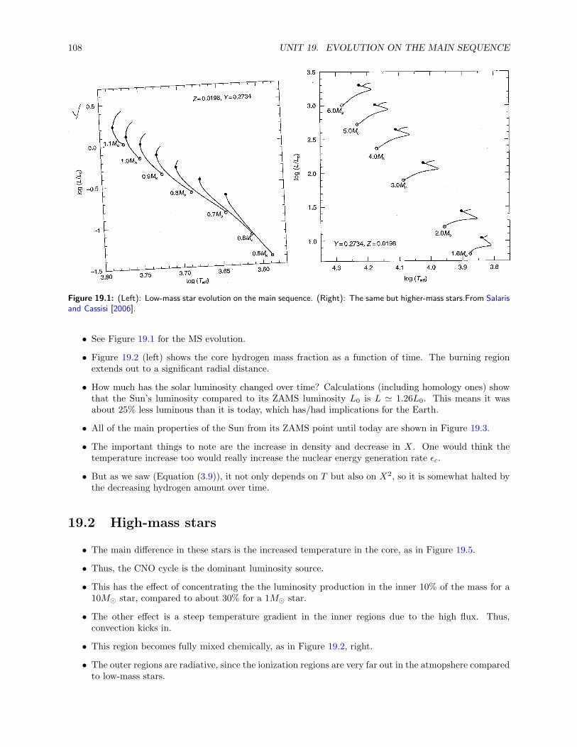
108 UNIT 19. EVOLUTION ON THE MAIN SEQUENCE
Figure 19.1: (Left): Low-mass star evolution on the main sequence. (Right): The same but higher-mass stars.From Salarisand Cassisi [2006].
• See Figure 19.1 for the MS evolution.
• Figure 19.2 (left) shows the core hydrogen mass fraction as a function of time. The burning regionextends out to a significant radial distance.
• How much has the solar luminosity changed over time? Calculations (including homology ones) showthat the Sun’s luminosity compared to its ZAMS luminosity L0 is L ≃ 1.26L0. This means it wasabout 25% less luminous than it is today, which has/had implications for the Earth.
• All of the main properties of the Sun from its ZAMS point until today are shown in Figure 19.3.
• The important things to note are the increase in density and decrease in X. One would think thetemperature increase too would really increase the nuclear energy generation rate ǫc.
• But as we saw (Equation (3.9)), it not only depends on T but also on X2, so it is somewhat halted bythe decreasing hydrogen amount over time.
19.2 High-mass stars
• The main difference in these stars is the increased temperature in the core, as in Figure 19.5.
• Thus, the CNO cycle is the dominant luminosity source.
• This has the effect of concentrating the the luminosity production in the inner 10% of the mass for a10M⊙ star, compared to about 30% for a 1M⊙ star.
• The other effect is a steep temperature gradient in the inner regions due to the high flux. Thus,convection kicks in.
• This region becomes fully mixed chemically, as in Figure 19.2, right.
• The outer regions are radiative, since the ionization regions are very far out in the atmopshere comparedto low-mass stars.
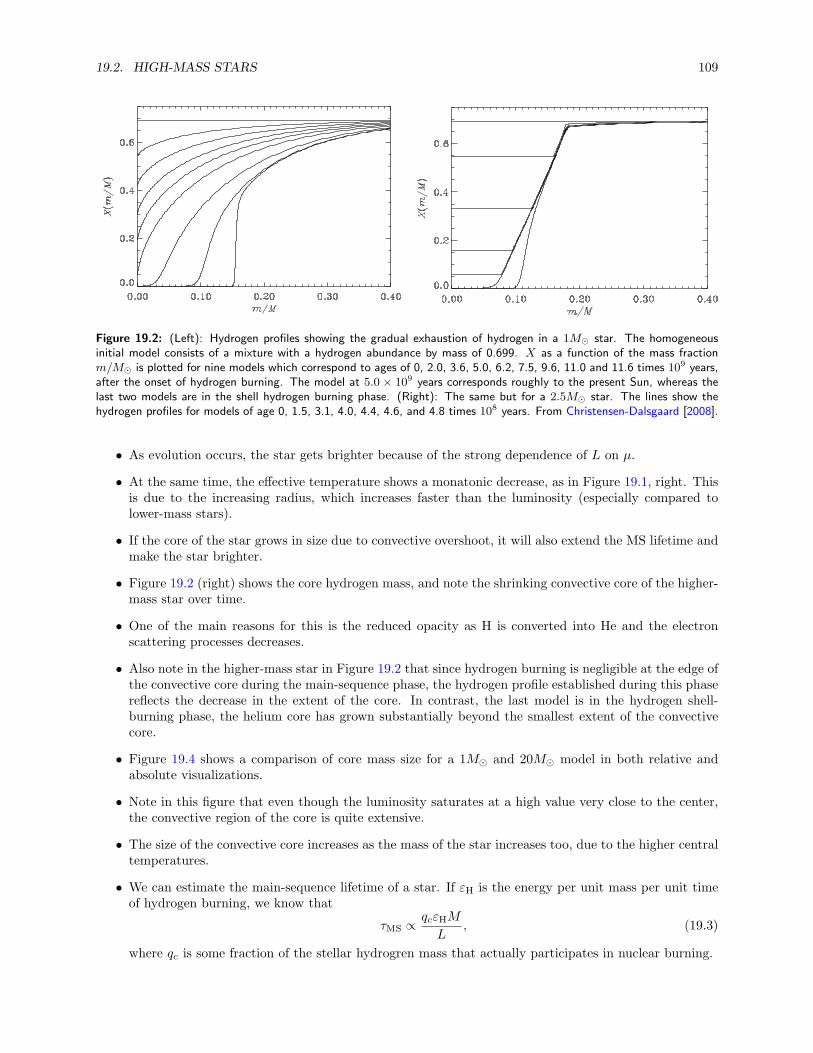
19.2. HIGH-MASS STARS 109
Figure 19.2: (Left): Hydrogen profiles showing the gradual exhaustion of hydrogen in a 1M⊙ star. The homogeneousinitial model consists of a mixture with a hydrogen abundance by mass of 0.699. X as a function of the mass fractionm/M⊙ is plotted for nine models which correspond to ages of 0, 2.0, 3.6, 5.0, 6.2, 7.5, 9.6, 11.0 and 11.6 times 109 years,after the onset of hydrogen burning. The model at 5.0 × 10⁹ years corresponds roughly to the present Sun, whereas thelast two models are in the shell hydrogen burning phase. (Right): The same but for a 2.5M⊙ star. The lines show thehydrogen profiles for models of age 0, 1.5, 3.1, 4.0, 4.4, 4.6, and 4.8 times 108 years. From Christensen-Dalsgaard [2008].
• As evolution occurs, the star gets brighter because of the strong dependence of L on µ.
• At the same time, the effective temperature shows a monatonic decrease, as in Figure 19.1, right. Thisis due to the increasing radius, which increases faster than the luminosity (especially compared tolower-mass stars).
• If the core of the star grows in size due to convective overshoot, it will also extend the MS lifetime andmake the star brighter.
• Figure 19.2 (right) shows the core hydrogen mass, and note the shrinking convective core of the higher-mass star over time.
• One of the main reasons for this is the reduced opacity as H is converted into He and the electronscattering processes decreases.
• Also note in the higher-mass star in Figure 19.2 that since hydrogen burning is negligible at the edge ofthe convective core during the main-sequence phase, the hydrogen profile established during this phasereflects the decrease in the extent of the core. In contrast, the last model is in the hydrogen shell-burning phase, the helium core has grown substantially beyond the smallest extent of the convectivecore.
• Figure 19.4 shows a comparison of core mass size for a 1M⊙ and 20M⊙ model in both relative andabsolute visualizations.
• Note in this figure that even though the luminosity saturates at a high value very close to the center,the convective region of the core is quite extensive.
• The size of the convective core increases as the mass of the star increases too, due to the higher centraltemperatures.
• We can estimate the main-sequence lifetime of a star. If εH is the energy per unit mass per unit timeof hydrogen burning, we know that
τMS ∝qcεHM
L, (19.3)
where qc is some fraction of the stellar hydrogren mass that actually participates in nuclear burning.

110 UNIT 19. EVOLUTION ON THE MAIN SEQUENCE
Figure 19.3: The changes in the solar properties at the center of a solar model. All variables are normalized with respectto the present Sun. From Christensen-Dalsgaard [2008].
• If εH and qc are roughly independent of total stellar mass, and we assume that L ∝Mγ as we showedbefore, then
τMS ∝M−(γ−1), (19.4)
where we found γ ≈ 3−5, and the relation is written to emphasize that the exponent is always negative,and main-sequence lifetime is inversely related to mass.
A note about very low mass stars
• Stars below about 0.3M⊙ are fully convective on the MS.
• They have large opacities due to low temperatures and very high densities.
• The densities are high because the stars need to contract to build up high enough temperatures fornuclear fusion.
• Only the PP-I chain can operate, so helium-3 is never really destroyed.
• But at the lower mass limit (high ρ), electron degeneracy kicks in.
• Conduction is very efficient here, which then cools the core below the minimum ignition temperatures.
• Some lithium or deuterium is burned, but these objects become brown dwarfs and cool down like whitedwarfs.
• The difference between them and WDs is that they are fully mixed chemically, and their degenerateelectrons do not move relativistically.

19.3. SUMMARY OF MAIN-SEQUENCE PROPERTIES 111
MassRadius
X(m/M),M = 1
L(m/M),M = 1
L(r/R), R =1
X(m/M),M = 20
L(m/M),M = 20
L(r/R), R =9.4
Hydrogenmassfraction
r/R∗, m/M∗
Normalized
luminosity
0 0.1 0.2 0.3 0.4 0.5 0.6
−15
−10
−5
0
5
10
15
0
0.5
1
0
0.5
1
Figure 19.4: Comparison of core sizes for 2 models (1M⊙ and 20M⊙) both with Xc ≈ 0.35 on the main sequence. Thetop panel shows the normalized luminosity as a function of normalized radius and mass. A horizontal line at 0.9Lmax willbe used to define the approximate core boundary. The blue lines are for the massive model, and red for the less massiveone. The low-mass model has a core that is fractionally larger than the core in the high-mass model. The gray solid anddashed lines are the hydrogen mass fraction, given on the right y axis. In the bottom panel, the surface (solid lines) andcore (dashed lines) boundaries are shown to scale in absolute masses and radii. On the left for the 9.4R⊙ model (blue),we see the core boundary in this space is almost exactly the same size of the entire low-mass star (red). In terms of mass,the core size of the massive star is larger than one solar mass.
19.3 Summary of main-sequence properties
• In general, the star regulates its nuclear burning rate to maintain hydrostatic equilibrium.
• If the rate increases for some reason, the star expands, thereby decreasing its temperature and density,reestablishing equilibrium.
• Mass rules of thumb:
– Below about 1.3M⊙ convective envelopes, above, radiative envelopes
– Below about 1.2M⊙ PP chain, above, CNO cycle
– Below about 1.5M⊙ late-type stars (F, G, K, M), above, early-type (O, B, A)
• Structure rules of thumb:
– Low-mass cores
∗ PP chain is sufficient to balance gravity
∗ Luminosity is not too steep, and energy flux is moderate
∗ Radiation is enough to carry out the luminosity from the core
∗ Core is radiative
∗ Since the PP chain has a low temperature dependence, the region of burning is relatively alarge mass fraction of the star, as in Figure 19.2, left.
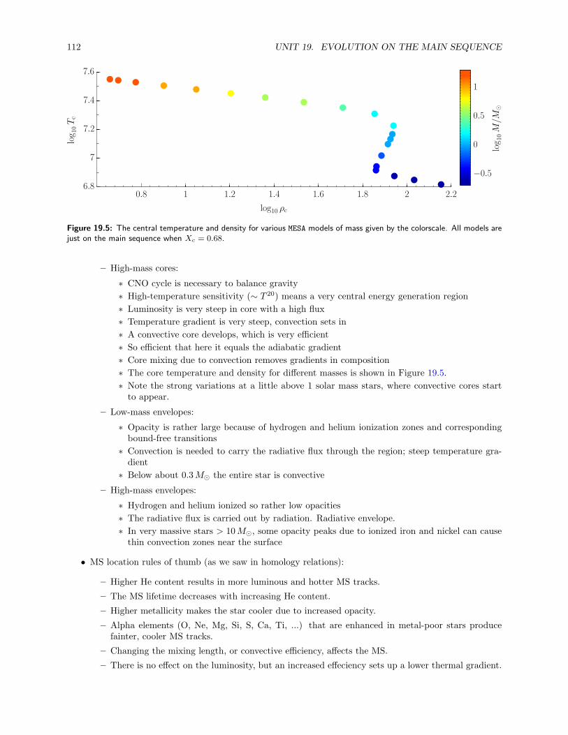
112 UNIT 19. EVOLUTION ON THE MAIN SEQUENCE
log10M/M
⊙
log10Tc
log10 ρc
0.8 1 1.2 1.4 1.6 1.8 2 2.2
−0.5
0
0.5
1
6.8
7
7.2
7.4
7.6
Figure 19.5: The central temperature and density for various MESA models of mass given by the colorscale. All models arejust on the main sequence when Xc = 0.68.
– High-mass cores:
∗ CNO cycle is necessary to balance gravity
∗ High-temperature sensitivity (∼ T 20) means a very central energy generation region
∗ Luminosity is very steep in core with a high flux
∗ Temperature gradient is very steep, convection sets in
∗ A convective core develops, which is very efficient
∗ So efficient that here it equals the adiabatic gradient
∗ Core mixing due to convection removes gradients in composition
∗ The core temperature and density for different masses is shown in Figure 19.5.
∗ Note the strong variations at a little above 1 solar mass stars, where convective cores startto appear.
– Low-mass envelopes:
∗ Opacity is rather large because of hydrogen and helium ionization zones and correspondingbound-free transitions
∗ Convection is needed to carry the radiative flux through the region; steep temperature gra-dient
∗ Below about 0.3M⊙ the entire star is convective
– High-mass envelopes:
∗ Hydrogen and helium ionized so rather low opacities
∗ The radiative flux is carried out by radiation. Radiative envelope.
∗ In very massive stars > 10M⊙, some opacity peaks due to ionized iron and nickel can causethin convection zones near the surface
• MS location rules of thumb (as we saw in homology relations):
– Higher He content results in more luminous and hotter MS tracks.
– The MS lifetime decreases with increasing He content.
– Higher metallicity makes the star cooler due to increased opacity.
– Alpha elements (O, Ne, Mg, Si, S, Ca, Ti, ...) that are enhanced in metal-poor stars producefainter, cooler MS tracks.
– Changing the mixing length, or convective efficiency, affects the MS.
– There is no effect on the luminosity, but an increased effeciency sets up a lower thermal gradient.

19.3. SUMMARY OF MAIN-SEQUENCE PROPERTIES 113
– This increases the effective temperature, and therefore the radius decreases.
• Evolution (on main sequence) rules of thumb:
– ZAMS to TAMS lifetimes are much shorter for high-mass stars
– Tracks on HR diagram are vertical for low-mass, and diagonal for high-mass stars
– Luminosity increases due to increase in molecular weight in core
– Low-mass stars have abundance changes in core that is smooth
– High-mass stars have discontinuous changes due to convective mixing (although core shrinkingcan smooth out the discontinuities)
– Below about 0.3M⊙ the core is completely mixed and stars live long
– Near the end of main-sequence evolution:
∗ Nearly isothermal core with zero luminosity
∗ Core is very hot from high µ
∗ At core boundary temperature is high enough for shell burning to occur
∗ The high T and large volume of the burning region leads to high shell L
∗ No thermal equilibrium, envelope expands

114 UNIT 19. EVOLUTION ON THE MAIN SEQUENCE

Unit 20
The Terminal-Age Main Sequenceand Subgiant Branch
20.1 Description of evolution movies
• From here on you can use the evolution movies to study the various stages that will be discussed.
• There are 2 stars considered of different masses, M1 = 1 M⊙ and M7 = 7 M⊙.
• Each star has 2 associated movies, one of the time evolution of general properties, and one depictingthe time evolution of interior profiles.
• They will be referred to as 1Ma, 1Mb, 7Ma, 7Mb, where “a” and “b” denote the history or profilemovie, respectively.
• A particular model in a movie will be denoted by, e.g., 1Mb-200, so the 200th model of movie 1Mb(not megabyte!)
20.2 TAMS
• The terminal-age main sequence (TAMS) is roughly the stage when the all the hydrogen is exhaustedfrom the very center of the star (not necessarily though throughout the whole core).
• This is about at model 280 for the 1 M⊙ star and model 1200 for the 7 M⊙ star.
• Observationally, we can only really talk about stars greater than about 0.8M⊙, since less massive starsare still on the main sequence (of course, we can use theory to talk about lower-mass stars).
• To summarize the previous material, as stars evolve on the main sequence they go above the ZAMSup and to the right or left depending on mass.
• Notice that this is only the case for chemically inhomogeneous models (if a star remained mixed andthe mean molecular weight increased with time throughout, it would evolve below the ZAMS for agiven mass, as we saw in our homology relations earlier).
• When the central hydrogen content reaches about Xc ≈ 0.05 (see points 3 in Figure 20.1 and 2 inFigure 20.2) for stars above about 1.1M⊙, the opacity is dropping (increased He), and the envelopeluminosity is greater than the energy generation in the core (not much H left!)
115

116 UNIT 20. THE TERMINAL-AGE MAIN SEQUENCE AND SUBGIANT BRANCH
Figure 20.1: Evolutionary tracks for low-mass Pop. I stars. Basically, points 1-3 are the ZAMS to TAMS. From Iben[1967b].
• The star shrinks on a Kelvin-Helmholtz time scale to make up for the excess luminosity, then theeffective temperature increases a bit (see § 20.3). This is a called overall contraction.
• This causes the little wiggle (or “hook”) on the HR diagram. Low-mass stars do not show this becausethey do not need to contract so much because the luminosity was never that great. See Figure 20.1(points 3 to 4) and 7Ma-1200-1220.
• The main difference is the higher-mass stars have a convective core.
• The higher-mass cores deplete H over larger regions, and thus the contraction is more drastic as tomaintain nuclear burning at the right level.
• Nonetheless, near the TAMS as Xc → 0 for all masses:
– Core is mainly filled with inert helium (too cool to burn, needs 108K)
– But there is a large Tc and µ
– Core is isothermal since ε→ 0 and then dT/dr → 0 (see Equation (13.18)).
– The temperature at the core boundary is high enough, however, to ignite leftover hydrogen
– The contraction has pulled in H to hotter and denser regions (still the shell), so the shell ignites!
– The shell burns H and adds He to the core, whose mass increases and it contracts more, heatingit up (eventually to ignite He later on)

20.3. SCHONBERG-CHANDRASEKHAR LIMIT 117
• All of this emphasizes the Shell-burning law: When a region within a burning shell contracts, theregion outside the shell expands; when the region inside the shell expands, the region outside the shellcontracts. We will see this behavior again and again.
• Despite many efforts, and the fact that numerical experiments show that this law is true, it is notobviously clear why it is the case.
20.3 Schonberg-Chandrasekhar Limit
• Let’s look at what’s happening in the core at the TAMS. Can it support the growing mass in theoverlying layers from outer core burning?
• In 1942 Chandrasekhar and Schonberg studied hydrostatic equilibrium for an isothermal He core andan ideal equation of state.
• Assume constant core temperature, and that the envelope provides a pressure Penv. The goal is tocompute the core pressure Pc.
• Consider hydrostatic equilibrium and multiply both sides by 4πr3 and integrate in core (recall Equa-tion (B.6)):
∫ Rc
0
4πr3dP
drdr = −
∫ Rc
0
ρGm
r24πr3dr = Eg,c (20.1)
• Integrate by parts and use ideal gas law
4πR3cPc − 3
MckBTc
µmu= Eg,c. (20.2)
• If we assume that the density is the mean core density ρ ≈ 3Mc/4πR3c , then
Eg,c ≈ −3
5
GM2c
Rc. (20.3)
• Solving everything for Pc, we get
Pc =3
4πR3c
(
MckBTc
µmu− 1
5
GM2c
Rc
)
(20.4)
• The core pressure must match the envelope pressure for equilibrium, and must adjust its radius to doso.
• Can it always do so? Its maximum value is when
Rc =4
15
GMcµmu
kBTc, (20.5)
which gives
Pc,max =10125
1024G3M2c
(
kBTc
µcmu
)4
. (20.6)
• As you can see, as the core mass increases, the core pressure will drop and at some point may fallbelow the envelope pressure.
• The mass at which this happens is the Schonberg-Chandrasekhar limit.
• We know from hydrostatic equilibrium that Penv ∝M2/R4.

118 UNIT 20. THE TERMINAL-AGE MAIN SEQUENCE AND SUBGIANT BRANCH
Figure 20.2: Paths in the HR diagram for a range of masses and solar metallicity. From Iben [1967a].
• From homology, we can find that Penv ∝ T 4c /M
2
• So the pressure at the surface of the core is independent of the core size.
• Using the right coefficients, it is then easy to show that
Mc
M≈ 0.37
(
µenv
µc
)2
. (20.7)
• If µenv = 0.6 and µc ≈ 1 (at solar composition), then the limit is roughly
Mc
M≈ 0.13. (20.8)
• Above this limit, which will likely occur for stars greater than 3M⊙:
– the isothermal core contracts rapidly
– the density increases, the temperature increases and nuclear reactions speed up in the shell
– This pushes in both directions and mass is lost in the shell, and burning is in a thin shell
– Even though the energy rate increases, the luminosity decreases a bit because of the mass loss inthe shell

20.4. THE SUBGIANT BRANCH 119
– Since the timescale is faster than the nuclear one, the stars become redder very quickly
– This leads to observational Hertzsprung gap (points 4 to 5 in Figure 20.2)
– Not many stars have time to be “observed”
– These are subgiant stars on the way to the bottom of the red-giant branch
– After the wiggle for our 7 M⊙ model, the core He mass is about 1 M⊙, above the limit computedabove.
• For low-mass stars (≤ 1.3M⊙), the helium core is somewhat degenerate and higher pressures arepresent, so this limit is not applicable and the approach to the RGB is slower.
• For higher-mass stars, the contraction happens very quickly and isothermal cores never actually havetime to set in.
20.4 The subgiant branch
• To summarize the above once again, in general, the move across the H-R diagram to the right definesthe subgiant branch (SGB).
• These are models 300-330 for the 1 M⊙ star, and 1200-1500 for the 7 M⊙ star.
• In general, cores are shrinking, envelopes are expanding, and surface temperatures are being reduced.
• Higher-mass stars have He core masses above the C-S limit.
• The envelope is adjusting to a new H-burning shell.
• The luminosity is larger as the burning takes place at a higher temperature than it was in the core
• With a large luminosity the shell has a difficult time radiating it (it will eventually become convective)
• But right now it absorbs the luminosity, heats up, and expands
• The Virial theorem shows some of the energy goes into expansion, not all of it makes it to the surface
• The slope of the luminosity in this move across the HR diagram depends on mass
• This stage should happen over the timescale of shell burning, a nuclear timescale ...
• But other influences may affect it, as will be discussed

120 UNIT 20. THE TERMINAL-AGE MAIN SEQUENCE AND SUBGIANT BRANCH
Unit 21
Towards and up the Red-GiantBranch
21.1 High-mass stars
• The red-giant branch (RGB) for the 7 M⊙ star is approximately models 1500-1750.
• As the star approaches the bottom of the RGB, opacities increase because of the cooling outer layers,and a convection zone near the surface appears. See 7Ma-1500 in the “Kippenhahn” panel.
• Mixing occurs near the surface.
• H− is the dominant opacity source.
• As the effective temperature continues to decrease, the luminosity finally begins to increase as convec-tion allows the luminosity to escape more readily.
• The shell burning power increases, but at the same time the mass in the shell decreases.
• The variation in the luminosity is interesting, as you can see that most of it is generated in a thin shellat about m ≈ 1.1 M⊙ in 7Mb-1530 in the “Summary Profile” panel.
• But note that near the center there is a small amount due to initial He burning that is beginning totake place. See the “Power” panel and the “text” panel.
• The subtle decrease in L in the envelope is due to expansion of the outer envelope where no nuclearsources reside and gravitational energy is “lost.”
• Note the core is no longer isothermal as a temperature gradient is required to carry out the luminositysupplied by He burning (“Summary Burn” panel).
• Continuing on, the convective envelope increases its extent in depth, carrying the luminosity to thesurface, as the core keeps contracting and the star keeps getting bigger.
• The convection almost reaches the burning shell at model 1600, but mixes the star and creates inter-esting abundance ratios for observers.
• A small convective core sets in with N being converted to O (recall one of the intermediate reactionsin the CNO cycle).
• When around model 1800 is reached, the central temperature and density are such that He burningvia the triple-alpha process takes place and is steady.
121

122 UNIT 21. TOWARDS AND UP THE RED-GIANT BRANCH
Helium core mass
Convection zone mass
Interior
mass[M
⊙]
Time [yr]×1010
0.8 0.85 0.9 0.95 1 1.05 1.1 1.15 1.20
0.2
0.4
0.6
0.8
1
Figure 21.1: How the base of the convection zone and the mass of the He core change with time for a 1M⊙ model. Thisillustrates how the first dredge up occurs.
• This occurs at about T = 108K.
• Now, instead of gravitational contraction in the core, nuclear energy again can support the star.
• The star “leaves” the RGB.
• It is a rapid increase in enery such that it causes the core to expland (energy can’t get carried out fastenough).
• There is still shell burning that is supplying most of the stellar luminosity, but it slows down a bit,and the luminosity decreases abruptly.
• Because of the shell-burning law too, the expanding core causes a shrinking star.
21.1.1 Low-mass stars
• The RGB phase for the low-mass star is models 330 to 4500. There are many more short time stepsin this case because of the degenerate condition in the core.
• The He core stars below the C-S limit, unlike the high-mass case.
• The density is also higher and so there is a degenerate component.
• The degeneracy provides enough pressure so that core contraction is not as extreme as for higher-massstars.
• The strong degeneracy is clear in the “temperature-density” panel.
• A convective envelope develops down to about 0.2M , and results in a sharp change in XH (“summaryprofile” panel).
• The convection mixes material from the surface to a point that once produced He from H. When itreaches its deepest extent, this is the first dredge up. What happens?
– The surface He abundance increases, and 3He and CNO elements get mixed in.
– A doubling of the surface 14N abundance.
– A reduction of 12C by about 30%.
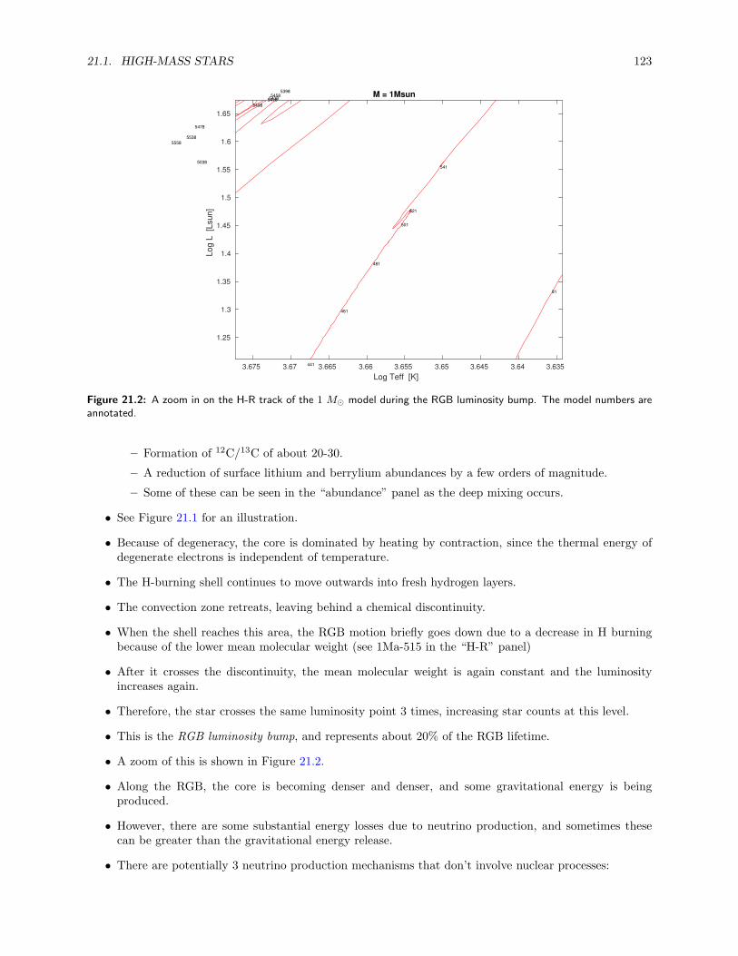
21.1. HIGH-MASS STARS 123
3.6353.643.6453.653.6553.663.6653.673.675
Log Teff [K]
1.25
1.3
1.35
1.4
1.45
1.5
1.55
1.6
1.65
Log L
[L
sun]
M = 1Msun
81
441
461
481
501
521
5415038
5398
541854385458
5478
5498
5538
5558
Figure 21.2: A zoom in on the H-R track of the 1 M⊙ model during the RGB luminosity bump. The model numbers areannotated.
– Formation of 12C/13C of about 20-30.
– A reduction of surface lithium and berrylium abundances by a few orders of magnitude.
– Some of these can be seen in the “abundance” panel as the deep mixing occurs.
• See Figure 21.1 for an illustration.
• Because of degeneracy, the core is dominated by heating by contraction, since the thermal energy ofdegenerate electrons is independent of temperature.
• The H-burning shell continues to move outwards into fresh hydrogen layers.
• The convection zone retreats, leaving behind a chemical discontinuity.
• When the shell reaches this area, the RGB motion briefly goes down due to a decrease in H burningbecause of the lower mean molecular weight (see 1Ma-515 in the “H-R” panel)
• After it crosses the discontinuity, the mean molecular weight is again constant and the luminosityincreases again.
• Therefore, the star crosses the same luminosity point 3 times, increasing star counts at this level.
• This is the RGB luminosity bump, and represents about 20% of the RGB lifetime.
• A zoom of this is shown in Figure 21.2.
• Along the RGB, the core is becoming denser and denser, and some gravitational energy is beingproduced.
• However, there are some substantial energy losses due to neutrino production, and sometimes thesecan be greater than the gravitational energy release.
• There are potentially 3 neutrino production mechanisms that don’t involve nuclear processes:

124 UNIT 21. TOWARDS AND UP THE RED-GIANT BRANCH
LHe
LH
Lsurface
log(L/L
⊙)
Time [Myr]
−0.2 0 0.2 0.4 0.6 0.8 1 1.2 1.4 1.6 1.8−4
−2
0
2
4
6
8
10
Figure 21.3: Helium flash for a 1M⊙ model. Time has been shifted to approximately the start of the flash, whichcorresponded to about 12 billion years. Note the decrease in the surface luminosity due to the expansion of the He coreand cooling of H-burning shell.
– Pair annihilation processes are when high-energy photons produce electron-positron pairs, thatannihilate and produce photons again, or, rarely, a neutrino-anti neutrino pair. This typicallyonly happens above one billion degrees.
– Photoneutrino processes from Compton scattering (electron + photon), when the photon becomesa neutrino-anti neutrino pair.
– Plasma processes when the photon traveling in a dense, degenerate environment becomes like aplasmon (having mass) and decays into a neutrino-anti neutrino pair.
• This can lead to the dL/dm = ε < 0 in the innermost regions.
• The maximum temperature is now located off center, in a shell. See 1Mb-3000 in the “summary burn”panel.
• Another cooling process is due to conduction from the degnerate electrons.
• In any case, the maximum temperature, wherever it is located, is increasing as time goes on becauseof the increasing He core mass and gravitational heating up of the inner layers.
21.2 Helium flash
• The He flash occurs after model 4000 or so.
• The temperature of the burning shell is increasing up the RGB, and when it reaches 108K, the helium
flash occurs.
• It coincides when the He-core mass is about 0.5 M⊙ (about 0.46 in our case), mostly independent ofthe total stellar mass.
• In a more massive star (which would be non-degenerate matter), the release of energy by nucelarburning would cause an increase in pressure and an expansion of material (core), and then cooling andan equilibrium would be restored, all rather smoothly.
21.2. HELIUM FLASH 125
• In the degenerate case, however, the gas pressure is basically independent of temperature (recall theEOS), and the high temperature causes no immediate reaction at the core.
• Instead the nuclear energy generation increases→ higher temperatures→ increased energy generation,. . .
• This is called a thermal runaway.
• The local luminosity in the core increases to about 100 billion L⊙ in a few hours! 1Ma-4300 in the“kippenhahn” panel shows the luminosity increase.
• See Figure 21.3.
• The new luminosity does not make it to the surface, however, but is absorbed by the overlying layers,which expand just outside the H-burning shell.
• Convection also sets in which spreads out the energy production over more mass layers.
• Eventually, the temperature gets so high that degeneracy is “lifted” at the point where the flash occurs(density is roughly constant). Recall Equation (8.8):
ρ
µe> 2.4× 10⁻⁸T 3/2.
• Interior to this first outer layer explosion, some smaller flashes may take place which eventually removesthe degeneracy everywhere. This is seen well around 1Ma-5650 in the “temperature-density” panel,where the degeneracy is removed.
• After this, the core expands (envelope contracts!) and cools, and an equilibrium of helium burning inthe core proceeds.
• The dynamical time scale of the star, because it is so large, is of the order of months.
• So the He flash in the core is not visible at the surface. The whole process takes on the order of onemillion years.
• See Figure 21.3 again.
• It is now on the helium burning main sequence, or better, the horizontal branch, or for seismologists,the red clump.

126 UNIT 21. TOWARDS AND UP THE RED-GIANT BRANCH
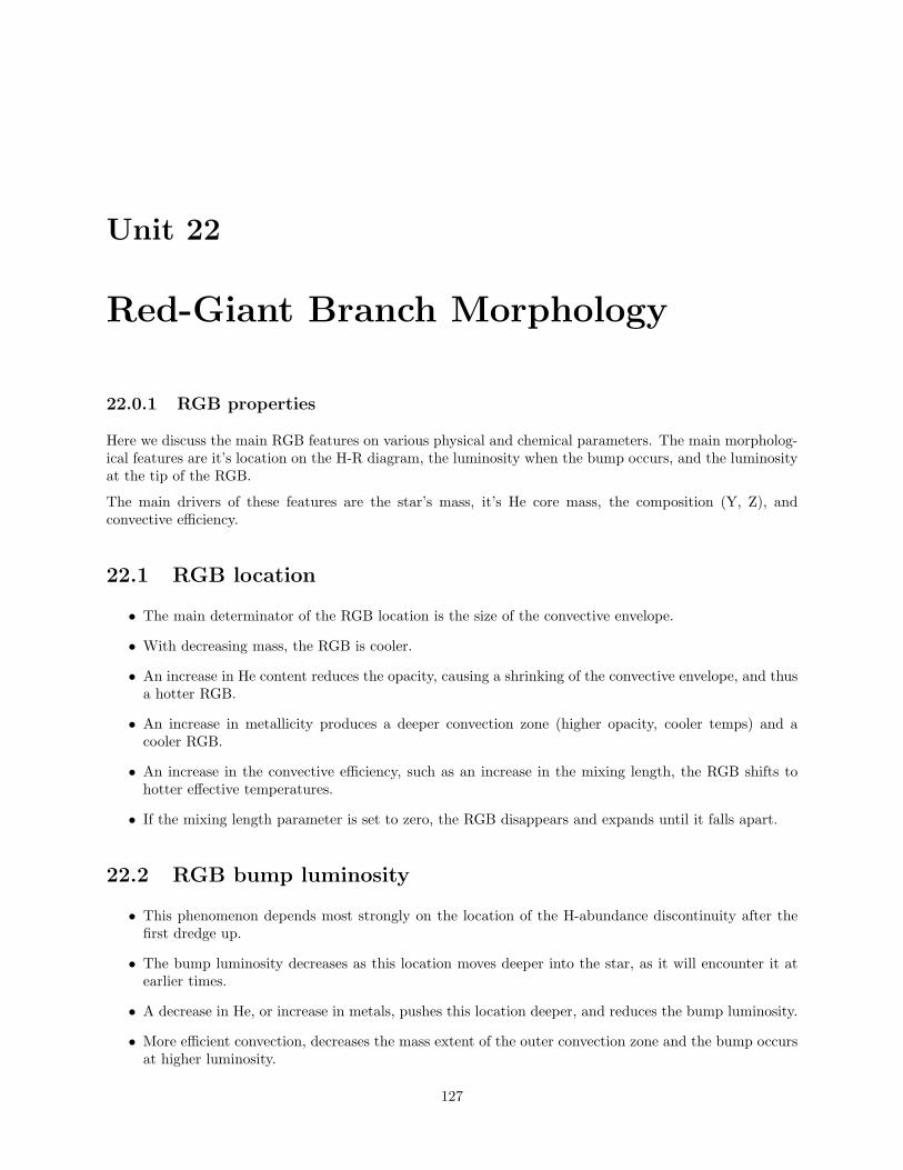
Unit 22
Red-Giant Branch Morphology
22.0.1 RGB properties
Here we discuss the main RGB features on various physical and chemical parameters. The main morpholog-ical features are it’s location on the H-R diagram, the luminosity when the bump occurs, and the luminosityat the tip of the RGB.
The main drivers of these features are the star’s mass, it’s He core mass, the composition (Y, Z), andconvective efficiency.
22.1 RGB location
• The main determinator of the RGB location is the size of the convective envelope.
• With decreasing mass, the RGB is cooler.
• An increase in He content reduces the opacity, causing a shrinking of the convective envelope, and thusa hotter RGB.
• An increase in metallicity produces a deeper convection zone (higher opacity, cooler temps) and acooler RGB.
• An increase in the convective efficiency, such as an increase in the mixing length, the RGB shifts tohotter effective temperatures.
• If the mixing length parameter is set to zero, the RGB disappears and expands until it falls apart.
22.2 RGB bump luminosity
• This phenomenon depends most strongly on the location of the H-abundance discontinuity after thefirst dredge up.
• The bump luminosity decreases as this location moves deeper into the star, as it will encounter it atearlier times.
• A decrease in He, or increase in metals, pushes this location deeper, and reduces the bump luminosity.
• More efficient convection, decreases the mass extent of the outer convection zone and the bump occursat higher luminosity.
127
128 UNIT 22. RED-GIANT BRANCH MORPHOLOGY
Figure 2. Left panel: the color–magnitude diagram of the HST data set.Figure 22.1: Left panel: the color–magnitude diagram of HST data for the globular cluster 47 Tuc. The RGB (includingthe RGBB) and the HB are all contained within their respective color–magnitude selection boxes. Right panel: magnitudedistribution of RG stars. The RGBB stands out as a prominent and significant peak at V = 14.51, with a normalization of(122± 14) stars. From Nataf et al. [2011], where they show the lifetime of the RGBB is different for different He amountsin the cluster stars.
• Another prediction of stellar evolution theory is that the lifetime of the RGBB is decreased as the Hecontent increases.
• Empirical support for this is alluded to in Figure 22.1 and the associated article.
22.3 RGB tip luminosity
• The luminosity at the tip of the RGB occurs when He is ignited.
• This typically happens at a well defined He core mass.
• For stars less massive than about 1.8M⊙, the mass of the He core at the flash does not depend on theoverall mass that much, and they all develop about the same amount of electron degeneracy in thecore.
• So the luminosity at the flash is about the same for these stars (all things otherwise being equal).
• For higher masses (about less than 3M⊙), the mass of the core is smaller and degeneracy is at lowerlevels, so the luminosity is reduced at the tip (ignition occurs earlier).
• For higher masses still, the luminosity starts to increase again as a result of the mass of the He coreincreasing again.
• An increasing He content increases interior temperatures and decreases electron degeneracy leading tolower He core mass and a lower tip luminosity.
22.3. RGB TIP LUMINOSITY 129
• An increasing metallicity also helps lower the He core mass, because shell H burning is more efficient.
• This heats the He core faster; however, the luminosity is higher with increasing metals since L isstrongly affected by the H-burning shell.
• Convection changes do not affect the tip luminosity since these don’t really change the mass of the Hecore.

130 UNIT 22. RED-GIANT BRANCH MORPHOLOGY
Unit 23
The Horizontal Branch
23.1 Quick tour of non-hydrogen nuclear reactions
• After H burning, we have He burning through the general triple alpha process
• There are, however, no stable elements with A = 5 or A = 8 (lithium is 7 and berrylium is 9).
• So it’s rather tricky for helium to burn (it can’t just interact with hydrogen or with itself).
• There is however an isotope of berrylium present from its formation from 2 helium nuclei
4He +4 He −→ 8Be (23.1)8Be +4 He −→ 12C+ γ. (23.2)
• The 8Be ground state energy is about 100keV higher than the ground state of 2 He nuclei, so it wantsto decay into that, to find the lowest ground state.
• Its lifetime is only about 10−16s.
• Since 8Be decays so quickly, the third helium must arrive in a short amount of time.
• But this is orders of magnitude longer than a scattering event.
• Additionally, at high temperatures the α+ α reactions increase rapidly.
• The key is that a nucleus of carbon is produced before the berrylium decay.
• Energy release is about 7.3MeV, or about 0.6MeV per nucleon, which is about an order of magnitudesmaller than CNO H burning.
• This all takes place in the T = 1− 2× 10⁸K range, and the reactions can be written
ε ≈ ε0Y3ρ2T ν , (23.3)
where ν = −3 + 4.4/T9.
• So at T = 108, ν ≈ 40!
• As density increases, this reaction is favored due to the quadratic dependence in the rate.
131
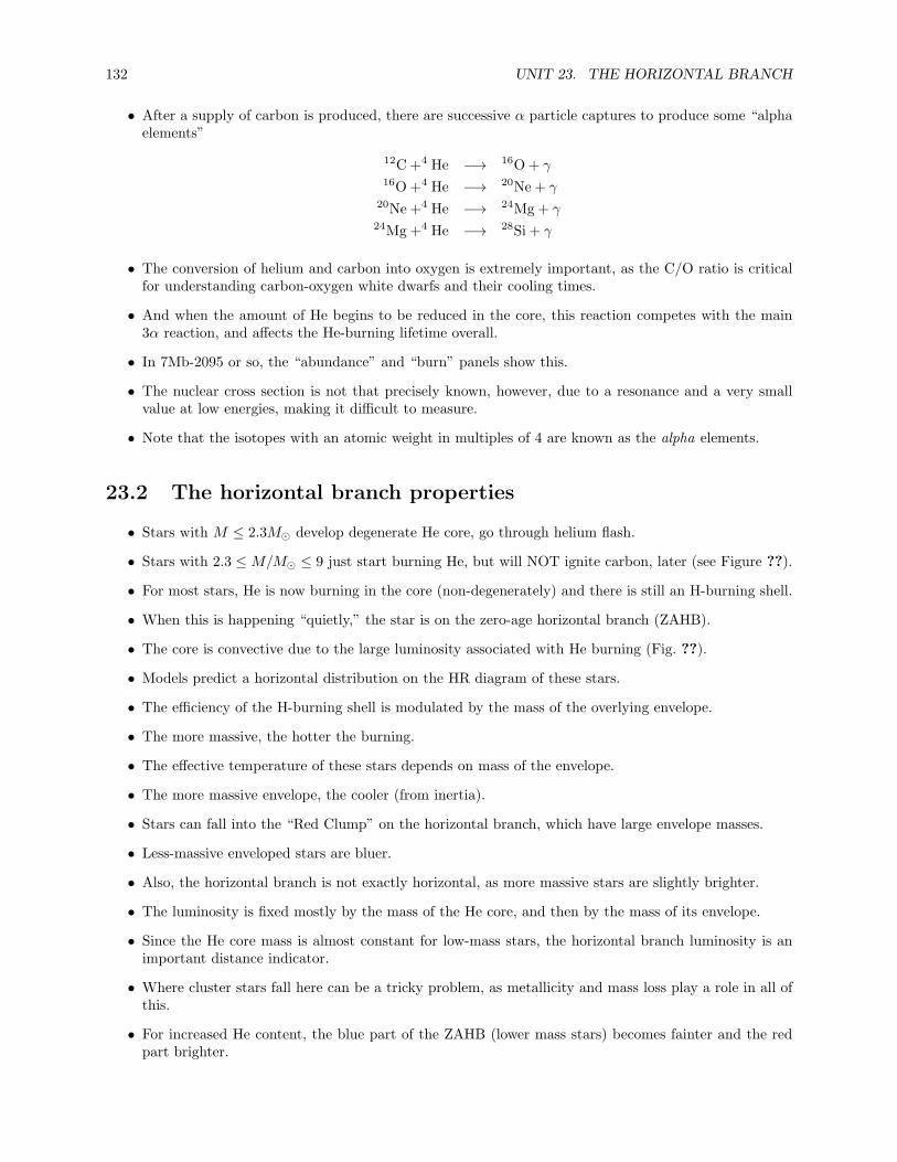
132 UNIT 23. THE HORIZONTAL BRANCH
• After a supply of carbon is produced, there are successive α particle captures to produce some “alphaelements”
12C+4 He −→ 16O+ γ16O+4 He −→ 20Ne + γ
20Ne +4 He −→ 24Mg + γ24Mg+4 He −→ 28Si + γ
• The conversion of helium and carbon into oxygen is extremely important, as the C/O ratio is criticalfor understanding carbon-oxygen white dwarfs and their cooling times.
• And when the amount of He begins to be reduced in the core, this reaction competes with the main3α reaction, and affects the He-burning lifetime overall.
• In 7Mb-2095 or so, the “abundance” and “burn” panels show this.
• The nuclear cross section is not that precisely known, however, due to a resonance and a very smallvalue at low energies, making it difficult to measure.
• Note that the isotopes with an atomic weight in multiples of 4 are known as the alpha elements.
23.2 The horizontal branch properties
• Stars with M ≤ 2.3M⊙ develop degenerate He core, go through helium flash.
• Stars with 2.3 ≤M/M⊙ ≤ 9 just start burning He, but will NOT ignite carbon, later (see Figure ??).
• For most stars, He is now burning in the core (non-degenerately) and there is still an H-burning shell.
• When this is happening “quietly,” the star is on the zero-age horizontal branch (ZAHB).
• The core is convective due to the large luminosity associated with He burning (Fig. ??).
• Models predict a horizontal distribution on the HR diagram of these stars.
• The efficiency of the H-burning shell is modulated by the mass of the overlying envelope.
• The more massive, the hotter the burning.
• The effective temperature of these stars depends on mass of the envelope.
• The more massive envelope, the cooler (from inertia).
• Stars can fall into the “Red Clump” on the horizontal branch, which have large envelope masses.
• Less-massive enveloped stars are bluer.
• Also, the horizontal branch is not exactly horizontal, as more massive stars are slightly brighter.
• The luminosity is fixed mostly by the mass of the He core, and then by the mass of its envelope.
• Since the He core mass is almost constant for low-mass stars, the horizontal branch luminosity is animportant distance indicator.
• Where cluster stars fall here can be a tricky problem, as metallicity and mass loss play a role in all ofthis.
• For increased He content, the blue part of the ZAHB (lower mass stars) becomes fainter and the redpart brighter.
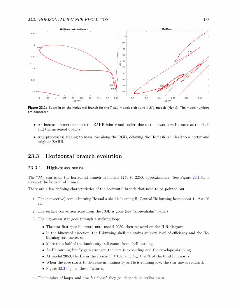
23.3. HORIZONTAL BRANCH EVOLUTION 133
3.653.73.753.83.853.93.9544.054.1
Log Teff
3.8
3.85
3.9
3.95
4
4.05
Lo
g L
M=7Msun, horizontal branch
1750
2050
2250
3.663.673.683.693.73.71
Log Teff
1.55
1.6
1.65
1.7
1.75
1.8
1.85
1.9
1.95
2
Lo
g L
M=1Msun
5600
5750
Figure 23.1: Zoom in on the horizontal branch for the 7 M⊙ models (left) and 1 M⊙ models (right). The model numbersare annotated.
• An increase in metals makes the ZAHB fainter and cooler, due to the lower core He mass at the flashand the increased opacity.
• Any process(es) leading to mass loss along the RGB, delaying the He flash, will lead to a hotter andbrighter ZAHB.
23.3 Horizontal branch evolution
23.3.1 High-mass stars
The 7M⊙ star is on the horizontal branch in models 1750 to 2250, approximately. See Figure 23.1 for azoom of the horizontal branch.
There are a few defining characteristics of the horizontal branch that need to be pointed out:
1. The (convective) core is burning He and a shell is burning H. Central He burning lasts about 1−2×10⁷yr.
2. The surface convection zone from the RGB is gone (see “kippenhahn” panel)
3. The high-mass star goes through a striking loop:
• The star first goes blueward until model 2050, then redward on the H-R diagram.
• In the blueward direction, the H-burning shell maintains an even level of efficiency and the He-burning core increases.
• More than half of the luminosity still comes from shell burning.
• As He burning briefly gets stronger, the core is expanding and the envelope shrinking.
• At model 2050, the He in the core is Y ≤ 0.5, and L3α ≈ 20% of the total luminosity.
• When the core starts to decrease in luminosity as He is running low, the star moves redward.
• Figure 23.2 depicts these features.
4. The number of loops, and how far “blue” they go, depends on stellar mass.
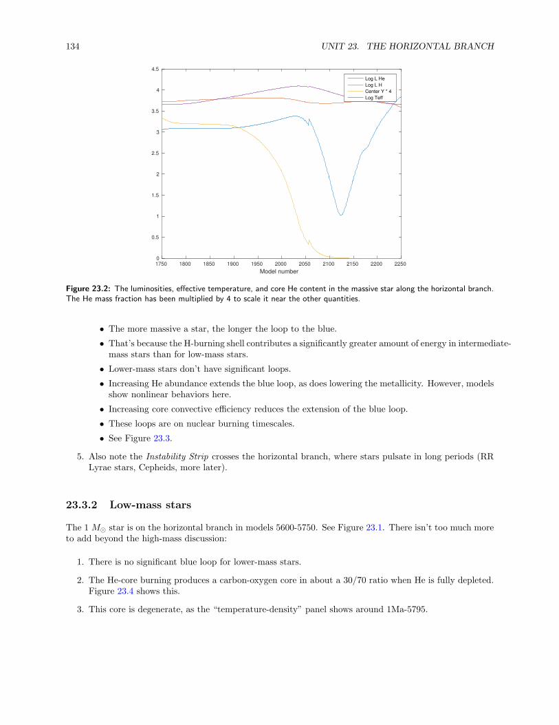
134 UNIT 23. THE HORIZONTAL BRANCH
1750 1800 1850 1900 1950 2000 2050 2100 2150 2200 2250
Model number
0
0.5
1
1.5
2
2.5
3
3.5
4
4.5
Log L He
Log L H
Center Y * 4
Log Teff
Figure 23.2: The luminosities, effective temperature, and core He content in the massive star along the horizontal branch.The He mass fraction has been multiplied by 4 to scale it near the other quantities.
• The more massive a star, the longer the loop to the blue.
• That’s because the H-burning shell contributes a significantly greater amount of energy in intermediate-mass stars than for low-mass stars.
• Lower-mass stars don’t have significant loops.
• Increasing He abundance extends the blue loop, as does lowering the metallicity. However, modelsshow nonlinear behaviors here.
• Increasing core convective efficiency reduces the extension of the blue loop.
• These loops are on nuclear burning timescales.
• See Figure 23.3.
5. Also note the Instability Strip crosses the horizontal branch, where stars pulsate in long periods (RRLyrae stars, Cepheids, more later).
23.3.2 Low-mass stars
The 1 M⊙ star is on the horizontal branch in models 5600-5750. See Figure 23.1. There isn’t too much moreto add beyond the high-mass discussion:
1. There is no significant blue loop for lower-mass stars.
2. The He-core burning produces a carbon-oxygen core in about a 30/70 ratio when He is fully depleted.Figure 23.4 shows this.
3. This core is degenerate, as the “temperature-density” panel shows around 1Ma-5795.

23.3. HORIZONTAL BRANCH EVOLUTION 135
Figure 23.3: Evolutionary tracks for intermediate-mass stars and higher, showing the extent of the blue loops.
5600 5620 5640 5660 5680 5700 5720 5740 5760 5780 5800
Model number
0
0.2
0.4
0.6
0.8
1
1.2
1.4
1.6
1.8M=1Msun, horizontal branch
Log L He
Log L H
Center Y
5600 5620 5640 5660 5680 5700 5720 5740 5760 5780 5800
Model number
0
0.1
0.2
0.3
0.4
0.5
0.6
0.7
0.8
0.9
1
Ma
ss f
ractio
n
M=1Msun, HB core mass fraction
Center C12
Center O16
Center Y
Figure 23.4: Horizontal branch properties for the 1 M⊙ star.

136 UNIT 23. THE HORIZONTAL BRANCH

Unit 24
Asymptotic Giant Branch
24.1 General overview
• The models representing the AGB for the 1 M⊙ star are approximately 5750-6000.
• The models representing the AGB for the 7 M⊙ star are approximately 2260-2495, although the fullAGB evolution was not computed.
• The H-R tracks are shown in Figure 24.1
• To summarize the approach to the AGB after horizontal branch evolution, the main driver is thathelium is less and less available for fusion in the core.
• As C and O builds up in the core, the mean molecular weight increases.
• The core contracts and increases in temperature (as before, in the Hertzsprung Gap).
• The contracting core releases gravitational energy and some gets converted to thermal energy and itreignites He in a shell around the core.
• The shell-burning law kicks in and the envelope expands, star moves to the red.
• There are 3 main characteristics of the AGB:
1. Nuclear burning takes place in 2 shells (with an He layer in between). As He burning in the coreexhausts, a new shell of He burning takes over in addition to the H-burning shell.
2. The luminosity is determined by the core C-O mass only.
3. A strong stellar wind due to radiation pressure develops causing significant mass loss.
4. s-process elements are produced.
• Let’s look at some of these.
24.2 Double-shell burning
• Some important interior profiles of the 7 M⊙ star on the AGB during double-shell burning are shownin Figure 24.2.
• The 2 burning shells are evident from the εnuc.
137
138 UNIT 24. ASYMPTOTIC GIANT BRANCH
3.543.563.583.63.623.643.663.683.73.72
Log Teff
1.5
2
2.5
3
3.5
4
4.5
Lo
g L
AGB of 1M and 7M
5597561756375657
567756975717
5737
5757
5777
5797
5817
5837
5857
58775897
59175937
595759775997
22002220
2240 2260
2280
230023202340
23602380
24002420
2440
Figure 24.1: Zoom of the asymptotic giant branch of the 1 M⊙ star (blue) and 7 M⊙ star (red).
• The luminosity is interesting and notable: Remember that dL/dm = 0 unless energy is being generated,so here we’d really have to account for εnuc + εgrav.
• The finite luminosity at the innermost region is from gravitational contraction of the core, as εgrav > 0.
• Between the 2 shells, the luminosity is decreasing slightly as that region expands (does work againstgravity), and εgrav < 0.
• In the outer part above the H shell, the envelope is also contracting, releasing gravitational energy.
• This is the shell-burning law in triple!
24.3 AGB evolution
• The core is too cold for C or O to burn (neutrinos are cooling it!). See 7Ma-2425 in the “kippenhahn”panel.
• Furthermore, for stars lower than about 10 M⊙, the carbon-oxygen core becomes degenerate (ourmodels do not get to that point).
• Thus, the contracting core does not heat up the gas and the high internal temperatures needed toignite the core are not reached.
• As the star reaches point continues, the shell-burning law has the core contracting (increasing in mass),the inner shell expanding, and the outer envelope contracting and increasing in effective temperature.
• But now the region between the two shell-burning sources has expanded sufficiently so that the tem-perature in the outer H-burning shell drops and extinguishes.
• Now there are only 2 distinct regions: the contracting core, and the now expanding envelope with Heburning in between (shell-burning law).
• Figure 24.2 (bottom panel) shows this.
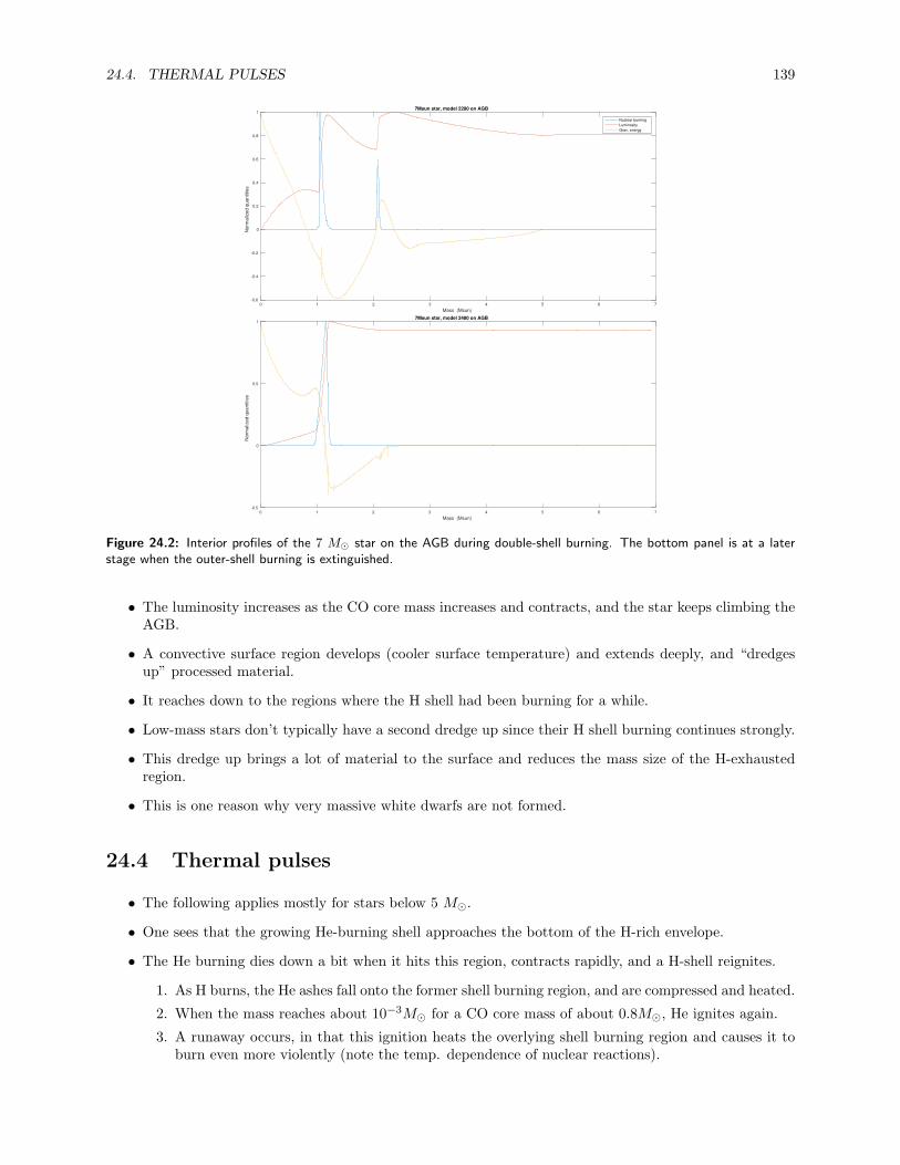
24.4. THERMAL PULSES 139
0 1 2 3 4 5 6 7
Mass (Msun)
-0.6
-0.4
-0.2
0
0.2
0.4
0.6
0.8
1
No
rma
lize
d q
ua
ntitie
s
7Msun star, model 2280 on AGB
Nuclear burning
Luminosity
Grav. energy
0 1 2 3 4 5 6 7
Mass (Msun)
-0.5
0
0.5
1
Norm
aliz
ed q
uantities
7Msun star, model 2480 on AGB
Figure 24.2: Interior profiles of the 7 M⊙ star on the AGB during double-shell burning. The bottom panel is at a laterstage when the outer-shell burning is extinguished.
• The luminosity increases as the CO core mass increases and contracts, and the star keeps climbing theAGB.
• A convective surface region develops (cooler surface temperature) and extends deeply, and “dredgesup” processed material.
• It reaches down to the regions where the H shell had been burning for a while.
• Low-mass stars don’t typically have a second dredge up since their H shell burning continues strongly.
• This dredge up brings a lot of material to the surface and reduces the mass size of the H-exhaustedregion.
• This is one reason why very massive white dwarfs are not formed.
24.4 Thermal pulses
• The following applies mostly for stars below 5 M⊙.
• One sees that the growing He-burning shell approaches the bottom of the H-rich envelope.
• The He burning dies down a bit when it hits this region, contracts rapidly, and a H-shell reignites.
1. As H burns, the He ashes fall onto the former shell burning region, and are compressed and heated.
2. When the mass reaches about 10−3M⊙ for a CO core mass of about 0.8M⊙, He ignites again.
3. A runaway occurs, in that this ignition heats the overlying shell burning region and causes it toburn even more violently (note the temp. dependence of nuclear reactions).
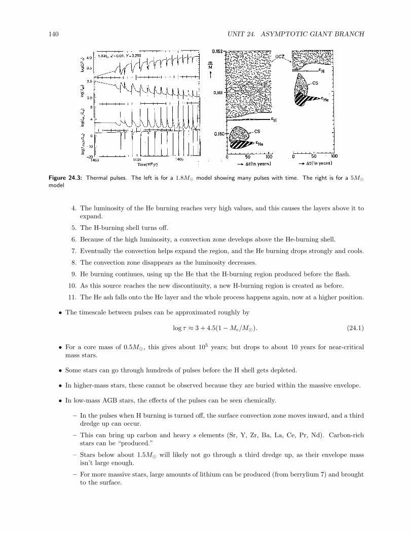
140 UNIT 24. ASYMPTOTIC GIANT BRANCH
Figure 24.3: Thermal pulses. The left is for a 1.8M⊙ model showing many pulses with time. The right is for a 5M⊙
model
4. The luminosity of the He burning reaches very high values, and this causes the layers above it toexpand.
5. The H-burning shell turns off.
6. Because of the high luminosity, a convection zone develops above the He-burning shell.
7. Eventually the convection helps expand the region, and the He burning drops strongly and cools.
8. The convection zone disappears as the luminosity decreases.
9. He burning continues, using up the He that the H-burning region produced before the flash.
10. As this source reaches the new discontinuity, a new H-burning region is created as before.
11. The He ash falls onto the He layer and the whole process happens again, now at a higher position.
• The timescale between pulses can be approximated roughly by
log τ ≈ 3 + 4.5(1−Mc/M⊙). (24.1)
• For a core mass of 0.5M⊙, this gives about 105 years; but drops to about 10 years for near-criticalmass stars.
• Some stars can go through hundreds of pulses before the H shell gets depleted.
• In higher-mass stars, these cannot be observed because they are buried within the massive envelope.
• In low-mass AGB stars, the effects of the pulses can be seen chemically.
– In the pulses when H burning is turned off, the surface convection zone moves inward, and a thirddredge up can occur.
– This can bring up carbon and heavy s elements (Sr, Y, Zr, Ba, La, Ce, Pr, Nd). Carbon-richstars can be “produced.”
– Stars below about 1.5M⊙ will likely not go through a third dredge up, as their envelope massisn’t large enough.
– For more massive stars, large amounts of lithium can be produced (from berrylium 7) and broughtto the surface.
24.5. PRODUCTION OF S ELEMENTS 141
24.5 Production of s elements
• As mentioned earlier, AGB stars are spectroscopically enriched in s-process elements.
• The s refers to slow neutron captures (compared to β decay).
• About half of the elements heavier than Fe are created by this process.
• You need neutrons to make these heavier elements, where the neutron eventually decays into a protonto make a stabler isotope.
• The neutrons densities needed are lowish, of order 10v per unit volume.
• Since at this stage there is a large abundance of N-14 in the intershell region, it gets converted to Neby
14N(α, γ)18F(β+, ν)18O(α, γ)22Ne. (24.2)
• If the temperatures at the base of the intershell region get to a few hundreds of MK, then 22Ne(α, n)25Mgcan provide a source of neutrons.
• For stars of initial mass < 3M⊙, it probably does not get hot enough for this reaction to occur.
• There may be some channels through carbon 13 that provide a high neutron density for low-mass AGBstars.
• However, this is still a very active area of research due to many physical uncertainties.

142 UNIT 24. ASYMPTOTIC GIANT BRANCH

Unit 25
Last Stages of Evolution: Low-MassStars
Here we discuss the late stages of evolution after the thermal pulses to the white dwarf.
25.1 Planetary Nebula
• AGB stars of low mass continute to brighten as their (outer) H shell approaches the surface.
• The thermal pulse number is set by the mass of the H envelope and the mass of the CO core.
• If the CO core exceeds about 1.4M⊙, non-degenerate, non-explosive carbon burning sets in and theAGB phase is over.
• Due to mass-loss processes during the AGB pulses, no star is really able to reach that core mass,because the H-burning shell stops when it’s at about 10−3M⊙ below the surface.
• The mass loss can be quite large, even 10−5 M⊙ yr−1
• These superwinds that are created speed off at 10 km s−1
• The mass loss could be explained by pulsations (Mira variables).
• The gas compression, and subsequent cooling and formation of molecules and dust grains, can trap theoutgoing radiation and get carried away.
• Anyway, however it happens, when the pulses stop, and the star evolves to hotter effective temperatures.
• The maximal luminosity depends on the star’s initial mass (and that of its envelope) and how muchmass it has lost.
• The H shell burning region approaches the surface and the effective temperature increases.
• An even faster stellar wind is produced, up to 2000 km s−1, which bumps up against the previous shellejecta - this produces interesting features in the planetary nebula.
• The shell is dusty and optically thick (masers).
• The envelope is irradiated by UV radiation from remaining hot central star (core).
143
144 UNIT 25. LAST STAGES OF EVOLUTION: LOW-MASS STARS
• The gas gets ionized and recombines quickly, giving distinct emission lines when the stellar remnantreaches about 30, 000K.
• A thin H-burning shell continues until the bluest point on the evolutionary track.
• Then, the H-rich envelope and He-rich layer contract quickly. A few scenarios are now possible:
1. All nuclear burning shuts off and the star cools as a WD.
2. The heating of the He from contraction leads to a thermal runaway, and the star goes back nearto the AGB (born again). Then does the same stuff and cools as a WD.
3. The heating of the envelope causes a H-burning runaway and the star is a self-induced nova. Theprocess can be dynamic and blow off all H layers to become a DB white dwarf. Or, the processcan be quiescent and it will burn H and start to cool down, possibly leading to another novaevent.
25.2 White Dwarfs
• Recall all the discussion in Sec. 10.4.
• Degenerate matter obeys polytropic relations P ∼ ργ .
• For non-relativistic particles, γ = 5/3.
• For relativistic particles, γ = 4/3.
• The cores of evolved degenerate stars like white dwarfs are dominated by electron pressure rather thanion pressure.
• That’s because µe ≈ 2 and µion ≈ 12, and P ∝ µ−1.
• Why are white dwarfs special?
• Let’s simply consider approximations to equilibrium with averages over the star, so
P
M=
GM
4πR4. (25.1)
• For a polytrope, replacing density by its average value
P ∼(
M
R3
)γ
. (25.2)
• The “pressure” term fp from equilibrium and the EOS, and the “gravity” term fg from equilibrium,are
fp ∼Mγ−1
R3γ; fg ∼
M
R4. (25.3)
• Their ratio must be 1 for equilibrium
f =fgfp∼M2−γR3γ−4. (25.4)
• This is M1/3R for γ = 5/3, and M2/3 for γ = 4/3.
• So consider a star less than some critical mass M < Mcrit and non-relativistic electrons. The star canget into an equilibrium by just adjusting R so that f = 1.

25.2. WHITE DWARFS 145
• If we increase M so that f > 1 (more gravity), R must decrease to regain equilibrium (hence moremassive WDs are smaller)
• Now consider relativistic electrons.
• We can only get equilibrium by setting the mass to a certain value M = Mcrit.
• If M < Mcrit, f < 1, and the pressure term is dominant and so the star expands so that the electronsbecome non relativistic.
• But if M > Mcrit and f > 1, the gravity term forces the star to contract. But this does not help,because f is independent of R!
• The star collapses without “finding” an equilibrium.
• Clearly, Mcrit is some limit.
• So again, consider a total degenerate equation of state then (recall Eq. 7.10)
P ≈ R
µeρT +Kγ
(
ρ
µe
)γ
. (25.5)
• γ depends on density and relativistic effects, being γ = 5/3 for ρ≪ 106 and γ = 4/3 for ρ≫ 106.
• Using polytropic relationships once can derive a critical mass that governs the future behavior of thecore of these dense stars
Mcrit =
(
K4/3
fG
)3/2
µ−2e , (25.6)
where f is the ratio of the mean density to the central density.
• The cricital mass is then identified as the Chandrasekhar mass (Equation (10.43)):
MCh
M⊙
=5.836
µ2e
= 1.456
(
2
µe
)2
. (25.7)
• It’s also important to see how the central temperature and density depend on this critical mass:
ρcµe
=1
8
(
K4/3
K5/3
)3(Mc
Mcrit
)2
≈ 2.4× 10⁵ g cm−3
(
Mc
Mcrit
)2
, (25.8)
Tc =1
R
K24/3
K5/3
(
Mc
Mcrit
)4/3
≈ 0.5× 10⁹(
Mc
Mcrit
)4/3
K. (25.9)
• For core masses below critical, maximum temperatures cannot exceed about 500 million K.
• In white dwarfs it is believed that the electrons are relativistic in the central part, but non-relativisticin the outer part.
• This changes the above results quantitatively, but not qualitatively.
• The mass of the core compared to the critical (Chandrasekhar) mass can be distinguised by 4 cases:
Case 1: If Mc < Mcrit ≈ MCh and if there is no significant envelope (from mass loss or just a smalloriginal mass), so that Mc will NOT approach MCh during shell burning, then the core becomesdegenerate, will cool, and the star becomes a white dwarf. Tc peaks. If it is a member of a binarysystem, then it can accrete enough mass to ignite carbon, which will detonate He and destroy thestar in a runaway, producing at Type I supernova
146 UNIT 25. LAST STAGES OF EVOLUTION: LOW-MASS STARS
Case 2: Initially if Mc < Mcrit but there remains an envelope such that shell burning Mc can grow toMCh, the core becomes degenerate and cools. However, ρc increases with Mc and carbon will beignited. This will happen for 4 . M/M⊙ < 8, and the stars will likely become white dwarfs aswell, but C-O white dwarfs.
Case 3: If Mcrit < M . 40M⊙, degeneracy does not happen. The core can heat up even more (because ofno degeneracy) and further nuclear reactions can occur. Eventually the core collapses leading toformation of a neutron star and ejection of the envelope. This is a Type II supernova. See nextsection.
Case 4: If Mc ≥ 40M⊙, the core also will burn C non degenerately. Black hole. See next section.
• In reality, almost all stars born with about 8M⊙ or less will lose significant mass and will not reachthe interior conditions to ignite carbon.
• Most WDs are observed at 0.6M⊙ with very little variation.
• The higher-mass stars will lose all of their envelope and become CO WDs.
25.3 Futher WD properties
• It can be shown through simple Virial arguments that white dwarfs cool (approximately) according tothe Mestel law
∆t ∝(
L
M
)−5/7
≈ 4.5× 10⁷
µi
(
LM⊙
L⊙M
)−5/7
[year]. (25.10)
• The ∆t represents the time for some change in luminosity.
• So higher mass WDs cool more slowly, due to more storage of energy.
• Increasing the ionic mean molecular weight decreases the evolutionary time, since there are fewer ionsin that case.
• Roughly, for a WD to reach 1/1000th of the solar luminosity, it would take 1 billion years.
• A more precise cooling law would treat the ions more properly, since the steady decreae in temperaturecauses Coulomb interactions to become more important.
• The specific heats ratio grows and the ions form a lattice: this is crystallization.
• The crystallization obviously affects the EOS, and therefore the cooling times.
• The envelopes of WDs canonically predicta He layer of ∼ 10−2Mtot above the CO core, surrounded bya H envelope of mass ∼ 10−4Mtot.
• Mass loss causes these notions to change.
• Metals are rarely observed due to atomic diffusion processes.
• Typically there are about 4 H WDs for every 1 non-H WD, but this varies widely with effectivetemperature, as evolutionary processes are still ongoing.
• The outer layers determine the opacity, and hence the cooling times.
• As WDs cool, they can develop convection zones as well.
• WDs can also be He core stars from an RGB progenitor that lost its envelope.
• There are also O-Ne WDs from higher-mass progenitors.
25.4. TYPE IA SUPERNOVAE 147
25.4 Type Ia supernovae
• Type I do not have visible hydrogen in its spectrum.
• The progenitor of these events are CO WDs that have accreted mass from a companion to exceed thecritical mass .
• The companion is likely on the RGB or AGB where mass can be transferred effectively.
• In one scenario two similar stars evolve through a common envelope, and the two CO WDs mergethrough angular momentum loss from gravitational waves.
• The resultant object is higher than the critical mass.
• This is the double-degenerate channel.
• No observational evidence of these massive systems has yet to be shown.
• In the single-degenerate case, the events that happen depend strongly on the mass-accretion rates ontothe low-mass star.
• For low rates, H burning on top of He layers produces an electron degenerate scenario, which canundergo explosive flashes.
• These are typically the classical Novae.
• Building up enough mass this way to reach the critical limit takes longer than a Hubble time, however.
• At moderate rates it can be shown that an explosion would occur for sub-Chandrasekhar mass objects.
• If enough He is accreted (either through H-burning above or from an He-rich companion), violentHe-ignition can occur which can detonate the CO core.
• Basically, WDs are unable to regulate their temperature the way they did in earlier stages (expandingand cooling). So runaway fusion occurs.
• The explosion models must give about 1051erg, as well as the production of heavy elements, such aslots of nickel.
• The explosive event is a shock wave whose speed depends on densities and abrupt thermal changes.
• Typical SNIa light curves rise rapidly and after about 20 days the light fades monotonically, withslighly different behavior in different bands.
• Almost all of them have a maximum absolute magnitude of −20 which declines linearly within 15 daysafter maximum.
• Thus, they are excellent standard candles.

148 UNIT 25. LAST STAGES OF EVOLUTION: LOW-MASS STARS
Unit 26
Last Stages of Evolution: High-MassStars
26.1 Nuclear burning
• Now we consider stars greater than 15M⊙.
• If we only focus on the core, the processes in the late stages follow the simple causes and effects of
. . .→ nuclear burning→ fuel exhaustion→ core contraction→ core heating→ . . . (26.1)
• At 500 million K, carbon burning can take place in the core, converting into Mg, Ne, and Na.
• Neutrinos from pair annihilation contribute a substantial amount to the luminosity (energy loss), evenmore than the nuclear burning.
• So the star contracts to make up the loss with gravitational energy.
• The convective C core is less massive for more massive stars, as neutrinos cause a considerable amountof mass loss.
• Eventually the burning moves to a shell of C and s-elements are produced.
• The core is now about 70% O, 25% Ne, and the rest Mg.
• Ne burning sets in .
• Oxygen burning can set in at 1.5 billion K.
• Eventually, the photons released in such reactions have such high energies that they can photo-disassociate surrounding nuclei.
• A large number of neutrons begin to be produced.
• Silicon burning sets in through interactions with alpha particles.
• Then it moves into the shell.
• The process stops at the iron group, and the last reaction is 52Fe capturing an alpha particle to makenickel.
• Further reactions would require energy to proceed. All reactions now are balanced by their inversereaction.
149
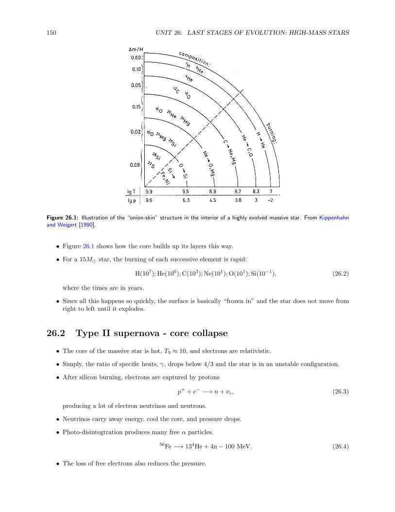
150 UNIT 26. LAST STAGES OF EVOLUTION: HIGH-MASS STARS
Figure 26.1: Illustration of the “onion-skin” structure in the interior of a highly evolved massive star. From Kippenhahnand Weigert [1990].
• Figure 26.1 shows how the core builds up its layers this way.
• For a 15M⊙ star, the burning of each successive element is rapid:
H(107); He(106); C(103); Ne(101); O(101); Si(10−1), (26.2)
where the times are in years.
• Since all this happens so quickly, the surface is basically “frozen in” and the star does not move fromright to left until it explodes.
26.2 Type II supernova - core collapse
• The core of the massive star is hot, T9 ≈ 10, and electrons are relativistic.
• Simply, the ratio of specific heats, γ, drops below 4/3 and the star is in an unstable configuration.
• After silicon burning, electrons are captured by protons
p+ + e− −→ n+ νe, (26.3)
producing a lot of electron neutrinos and neutrons.
• Neutrinos carry away energy, cool the core, and pressure drops.
• Photo-disintegtration produces many free α particles.
56Fe −→ 134He + 4n− 100 MeV. (26.4)
• The loss of free electrons also reduces the pressure.

26.2. TYPE II SUPERNOVA - CORE COLLAPSE 151
• The core collapses from overlying weight on the scale of a few seconds.
• This collapse halts when the neutron degeneracy pressure kicks in (ρ ≈ 1015 g cm−3) - note that thisis nuclear matter density! And 40km in size!
• Energy release of about 1053erg from change in gravitational energy GM2/∆R. Where does it go?
• This is as much light as a galaxy shines at for decades.
• In one scenario, most of the light is not released however, but goes into the kinetic energy of a shock.
• This propagates outward into the outer core region that is still collapsing.
• Naively, this might blow off the outer layers, but that does not happen.
• In the more accepted scenario, the increased core density causes it to be optically thick to neutrinos.
• They begin to deposit their energy into the material.
• This causes the outward shock that blows off the star’s layers.
• This is the core-collapse Type II event.
• Heavy nuclei are created through neutron capture (s and r processes)
• Just to note, the neutrino cross section is extremely small, and its mean free path is
ℓν =1
nσν≈ 1
µeA
(
ρ
µe
)−5/3
1.7× 1025 cm. (26.5)
• µe = 2, A = 100, and a density of about 1010, ℓν ≈ 107cm, which is contained withing the collapsingcore
• So neutrinos do not escape without interaction.
• About 1% of the energy goes into the outward motion, and 1% of that gets released as photons
• So only about 1049 erg of energy gets radiated over a few months
• We observe these supernova because hydrogen lines are present.
• The collapse occured when a H-rich envelope still existed.
• If the initial star was M ≥ 25M⊙, the remnant is likely a neutron star.
• For higher masses, it is too much to be supported by neutron degeneracy pressure.
• The object then becomes a black hole.
• If the initial star was over 100M⊙, or a core He mass of about 40M⊙, a different scenario might takeplace.
• After He burning the thermal environment produces electron-positron pairs, reducing the specific heatso that γ < 4/3.
• The star immediately starts to collapse and subsequent burning is not enough to halt the collapse.
• The star produces a black hole in a pair-instability supernova.
152 UNIT 26. LAST STAGES OF EVOLUTION: HIGH-MASS STARS
26.3 Neutron star
• Masses between 1.2 and 2.5M⊙ and R ≈ 10km
• The mass-radius relationship for neutron stars in each case is (derived from our polytropic equations):
M =
(
15.12 km
R
)3
M⊙; non− relativisitic (26.6)
M = 5.73M⊙ ≡ MNSCh; relativisitic (26.7)
• However, tne maximum mass of a neutron star depends on the existence of a general-relativisticinstability (interactions between nucleons)
• This likely takes place well before the MCh for a neutron star, hence the ∼ 3M⊙ limit
• Most neutron star observations are in a very narrow range of masses Mns = 1.35± 0.04M⊙.
• The neutron-degenerate material creates mostly an isothermal environment.
• They cool down faster than WDs.
26.4 Black hole
• For Type II remnant > 2.5M⊙, or a progenitor > 25M⊙, a black hole is produced.
• The radius, determined from the escape velocity, is:
R = 2GM
c2= 2.95× 10⁵
M
M⊙
[cm]. (26.8)

Unit 27
Instability Strip and Pulsations
27.1 Background
• We first consider the types of stars that display pulsations.
• Figure 27.1 shows where many of these types of stars lie on the H-R diagram.
• The Cepheid instability strip is the main thing to pay attention to, which spans from high luminositydown to the main sequence.
• Here, there are Cepheids, RR Lyrae, and δ-Scuti stars, etc.
• The instability strip is very narrow, and we’ve learned that it’s hard to “catch” stars in the HertzsprungGap.
• The higher luminosity stars must therefore be more massive, going through their “loops,” which occuron a much longer timescale.
• These stars have pulsations excited by an opacity mechanism, explained later.
• Typically only one mode is observed for the more luminous stars (Cepheids and RR Lyrae), a radialmode.
• For the stars near the main sequence, such as the δ Scuti, γ Dor, slowly pulsating B stars (SPB) andβ Cephei, multiple modes are observed.
• δ Scutis have masses around 1.5 − 2.5M⊙ (convective cores, F stars), and have periods of an hour orso.
• This makes their observation a bit difficult.
• They are expected to have acoustic pulsations.
• The Mira variables are related to the AGB stage of stars.
• The “EC14026” stars are subdwarf B variables (SdB), believed to also pulsate from an opacity mech-anism (related to iron).
• These interesting stars are on the horizontal branch as core helium burning is proceeding.
• However, at 35,000K they are much bluer than most HB stars.
• They have somehow lost most of their H envelope beforehand.
153

154 UNIT 27. INSTABILITY STRIP AND PULSATIONS
Figure 27.1: Schematic Hertzsprung-Russell diagram illustrating the location of several classes of pulsating stars. Thedashed line shows the zero-age main sequence, the continuous curves are selected evolution tracks, at masses 1, 2, 3, 4, 7,12 and 20M⊙, the dot-dashed line is the horizontal branch and the dotted curve is the white-dwarf cooling curve. FromChristensen-Dalsgaard [2003].
• The “Irr” irregular pulsators show strange amplitude variations, but are now known as red giantsolar-like pulsators.
• White dwarfs pulsate all along the cooling phase (ZZ Ceti as they are sometimes known).
• They are pulsating with periods up to 10 min, much longer than their dynamical timescales.
• Likely pulsating with internal gravity modes.
• Finally, solar-like oscillations are expected in stars < 7000K, due to convective mechanisms operatingnear the surface.
• Pulsations can be observed by intensity fluctuations, doppler-velocity observations, and line-profilevariations (for nonradial modes).
27.2 Pulsation mechanisms
• The adiabatic sound speed of stellar interiors is given as
c2s =γp
ρ, (27.1)
27.2. PULSATION MECHANISMS 155
where again
γ =d ln p
d ln ρ.
• The most fundamental period of pulsations is inversely proportional to the mean density of a star
Π ∝ ρ−1/2. (27.2)
• This can be obtained from hydrostatic equilibrium and some basic principles, but can more easily beseen just from the dynamical timescale, Eq. (1.11):
tdyn =
(
R3
GM
)1/2
∝ ρ−1/2,
which is its direct counterpart.
• A rigorous treatment can provide an exact equation for Eq. (27.2).
• Radial modes are standing waves, and the fundamental mode has only a node at the center and thesurface of the star
• After that, we have overtones of the fundamental mode, with nodes placed internally to the star
• Cepheids are observed to pulsate in fundamental radial modes
• Their magnitude, temperature, radius, and surface velocity change as a function of time
• The temperature varies by about 1000 K
• The radius by about 10%
• The star is brightest when it is expanding after its minimum radius was reached
• There is a phase lag between the radius and the luminosity
• We do know that as stars pulsate, energy is lost in each pulsation cycle, as most of the volume of thestar damps it
• These pulsations can only continue of there is a driving mechanism that is feeding energy into thepulsation, at least as much that has been damped out
• The first proposition to explain such pulsations was that of a heat engine (convert thermal to mechanicalenergy)
• Pulsations are driven if positive work is done, and damped if negative work is done (on a layer, andthroughout the star)
• Eddington postulated a valve mechanism, whereby a layer of a star could block energy that would thenpush the layer outward.
• After expansion, the blocked region would allow energy to pass through and the cycle would start again
• So, simplistically, the driving mechanism is this
– The increase in opacity due to ionization halts the energy flow
– The absorbed energy ionizes and eventually heats the gas and the pressure increases, pushing thelocal layer outward past its equilibrium point (expansion)
– This ionization process reduces the opacity since now the density decreases (expansion) and thetemperature does not decrease too rapidly because of partial recombination (κ ∝ ρT−3.5)
– Radiation can now flow freely, the gas cools and can no longer support the overlying weight

156 UNIT 27. INSTABILITY STRIP AND PULSATIONS
– The star contracts and compresses and the density increases
– The opacity is thus raised again and the whole process stars over
• This is the κ mechanism
• The other main driving mechanism is stochastic driving due to convection near the surface
• These modes are typically stable, but there is a lot of acoustic energy in outer convection zones suchthat this noise is transferred to the energy of global oscillations
27.3 Ionization zones
• The ionization zones being considered are hydrogen and the first and second ionization levels of helium
• These occur at about 10,000-20,000K
• To fully ionize helium requires about 40,000K
• For hot stars, with a Teff ≥ 7500K, these ionization zones are near the surface
• There is not much mass here and oscillations cannot be driven strongly
• In cooler stars with Teff . 5500K, these zones occur deeper
• However, convection is occuring in these envelopes
• Convection is efficient and does not allow a sufficient “blocking” of the radiation or energy flux
• Pulsations may not therefore occur from this mechanism, and the red edge of the instability strip isdefined
• Most of the driving is due to ionizing He zones from modeling
• The H ionization zones are interesting and since they lie above the He zones, they “carry” the emergentluminosity outward
• Thus the phase lag in the luminosity-minimum radius relations
• Note that these ionization zones alter the value of Γ1, and lower the adiabatic gradient.
• These regions can often be unstable to convection which can also drive pulsations through convectiveflux
• For β Cephei stars, it is Fe-group elements doing the driving


![fall2019-centos7-logbrazil.minnesota.edu/examples/ex/fall2019-centos7-log.pdfFile Edit View Search Terminal Help [preuss@log91 —]$ journalctl Hint: You are currently not seeing messages](https://static.fdocuments.us/doc/165x107/5fdbc4c85abb1969c4345751/fall2019-centos7-file-edit-view-search-terminal-help-preusslog91-a-journalctl.jpg)


![Current DINNER [FALL2019] - Chino Latinochinolatino.com/wp-content/uploads/menu-2019.10.pdf · 2019-10-11 · Title: Current DINNER [FALL2019].ai Author: manager Created Date: 10/11/2019](https://static.fdocuments.us/doc/165x107/5f58a84a0547bf16637069c3/current-dinner-fall2019-chino-2019-10-11-title-current-dinner-fall2019ai.jpg)