ASTEC

(presentation Aarhus Oct. 2005)

Aarhus Stellar Evolution CodeJørgen Christensen-Dalsgaard

Danish AsteroSeismology CentreDepartment of Physics and Astronomy

Aarhus University

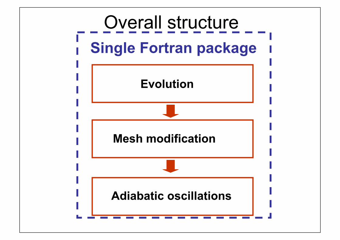
Overall structure

Evolution

Mesh modification

Adiabatic oscillations

Single Fortran package

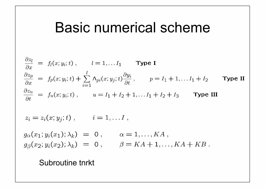
Basic numerical scheme

Subroutine tnrkt

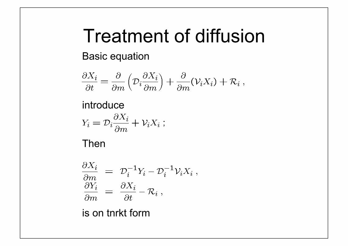
Treatment of diffusionBasic equation

introduce

Then

is on tnrkt form

Discretization

• Second-order spatially centred differences

• Time-centred differences in evolutionequation for H

• Backwards differences for other elements, ingeneral, and in energy equation (for stability)

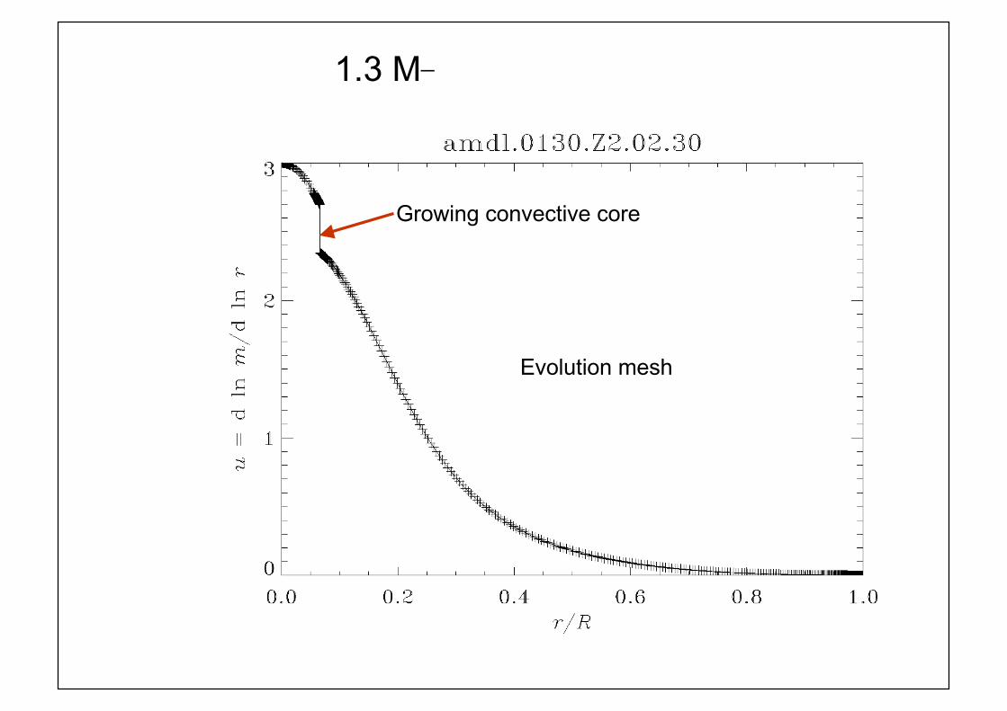
Implementation details: Mesh

The scheme for defining the mesh is broadly as described by CD82;however, a very dense mesh is used near the boundary of a possibleconvective core.

Most calculations for CoRoT comparison used 601 points (betweencentre and photosphere). However, also tests of effect of increasingnumber of meshpoints.

Distribution of meshpoints

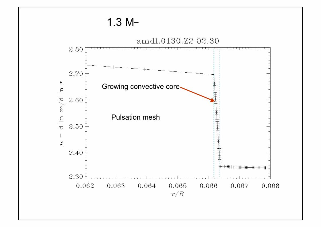
Implementation details: Pulsationmesh

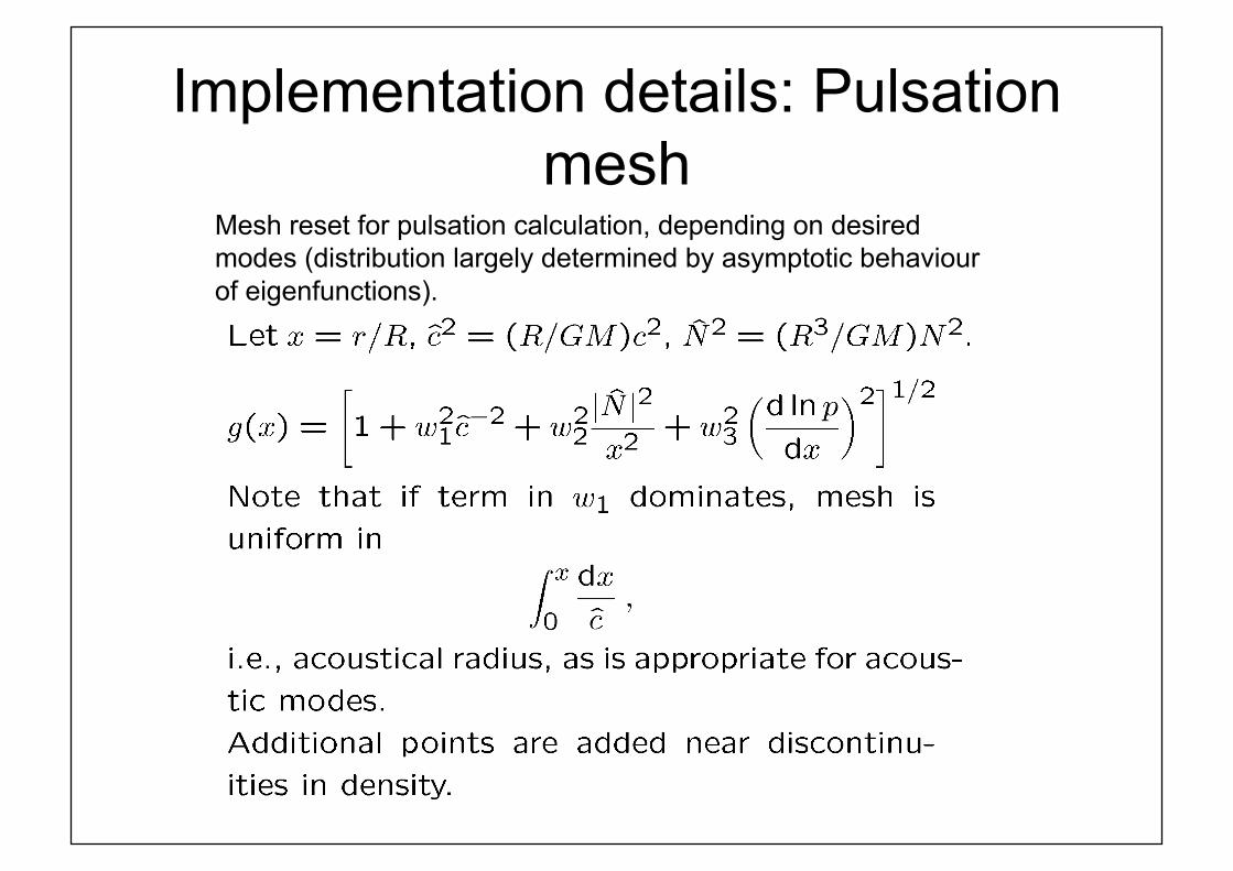
Mesh reset for pulsation calculation, depending on desiredmodes (distribution largely determined by asymptotic behaviourof eigenfunctions).

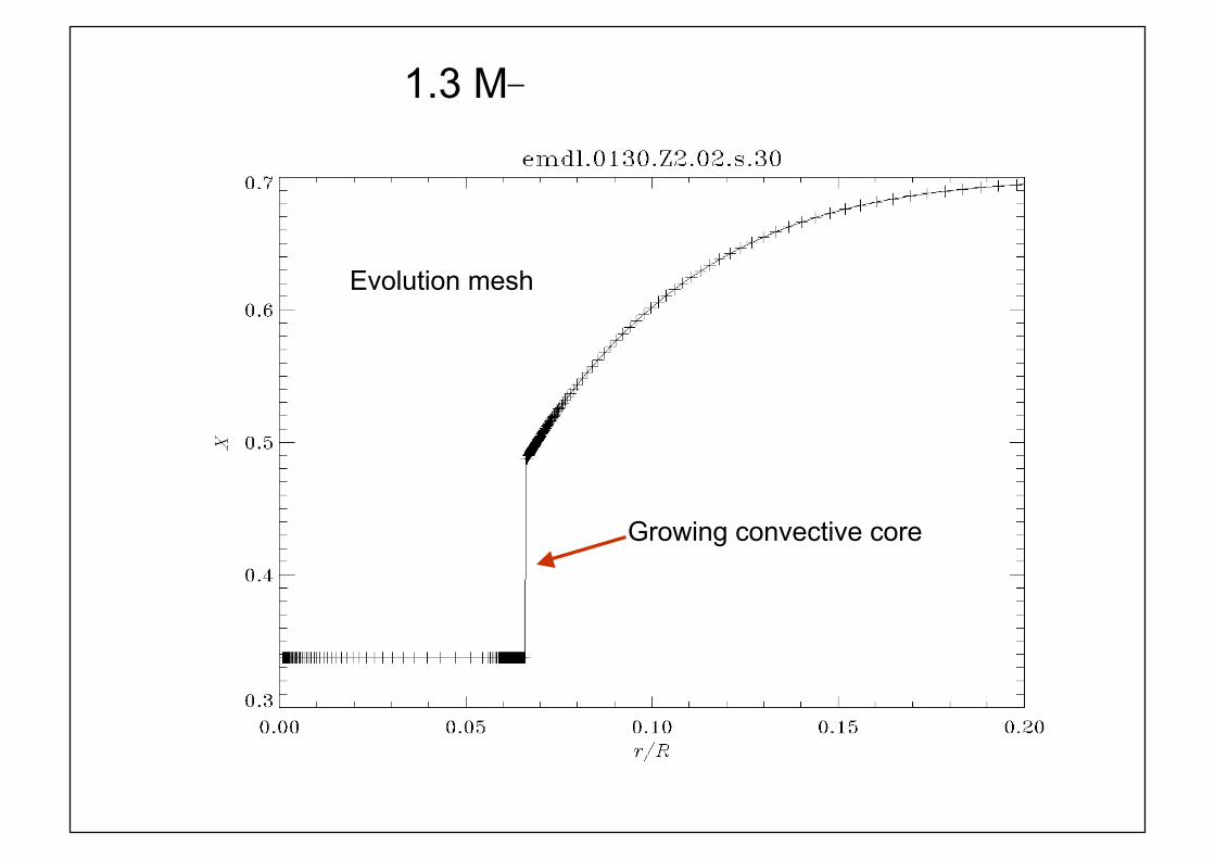
1.3 M¯

Evolution mesh

Growing convective core

1.3 M¯

Evolution mesh

Growing convective core

1.3 M¯

Evolution mesh

Growing convective core

1.3 M¯

Pulsation mesh

Growing convective core

1.3 M¯

Pulsation mesh

Growing convective core

Implementation details:Timestep

The timestep is set based on relative (or log10) changes in severalquantities being limited to be below a specified limit Δ ymax.

Changes in the hydrogen abundance in a convective core arescaled by a factor 5, to compensate for the rather crude numericaltreatment of the core composition. As a result, more timesteps areused in models with a convective core.

In the present case, typically 200 steps are required to reachexhaustion of hydrogen at the centre, in models with a convectivecore, and 30 - 40 steps in a model without (this small number is alsoa consequence of the crude treatment of the nuclear network).

Implementation details: equationof state

OPAL 2001 tables, for the appropriate value of Z (= 0.02 or 0.01).

Using the OPAL interpolation scheme.

Implementation details: opacity

OPAL 1996 tables, with Alexander low-temperature values. Houdekinterpolation scheme. The heavy-element abundance is taken to bethe initial value, regardless of the changes due to nuclear reactions.

(In models with diffusion and settling, these effects on heavy elementsare decoupled from the nuclear changes in composition, for now. Themodified heavy-element abundance is used for the opacity but not,usually, for interpolated equations of state.)

Implementation details:nuclear reactions

For Toulouse comparison: nuclear reaction parametersgenerally from Bahcall & Pinsonneault (1995).

NACRE now implemented. Corrected 21/10/05!

Salpeter weak screening.

Implementation details:treatment of convection

Böhm-Vitense (1958) mixing-length treatment, probably withHenyey et al. (1965) detailed parameters. (The specification ofthese parameters seems a little uncertain.)

Turbulent pressure is not included.

Implementation details:treatment of atmosphere

Integration of hydrostatic equation assuming the grey Eddington T(τ)relation: T = Teff [3/4*(τ + 2/3)]0.25, starting at τ = 0.01 and matchingwhere T = Teff (τ = 2/3).

Note that there are potential problems with the treatment of radiationpressure in the atmosphere, certainly for relatively massive (and hot)stars.)

Implementation details: initialmodel, chemical evolutionThe models start from the ZAMS (PMS evolution has been used in thecode, but not tested with care).

Chemical evolution is integrated with the general solution of the structureand evolution equations (tnrkt).

A separate treatment is used for the chemical evolution of theconvective core, using the averaged reaction rates. This is carried out inparallel with the Henyey iteration, although occasionally with fixes toensure convergence (freezing the properties of the core).

CN part of the CNO cycle is assumed to be in nuclear equilibrium at alltimes; initial 14N abundance includes also the original 12C abundance.The conversion of 16O into 14N is taken into account. The initialabundances of 14N and 16O, relative to the heavy-element abundance,are 0.2337 and 0.5154. (May well need to be changed, to meetspecifications.)

Implementation details:treatment of 3He

Original models (for Toulouse):3He is assumed to be in nuclear equilibrium at all times.

Recent modelling (and always used in solar case):

Set ZAMS 3He abundance by evolving abundance for time τ3at constant conditions, starting from initially constantabundance.

Typical value (for solar models): τ3 = 5 £ 107 years

Also try τ3 = 107 years for 0.9 M¯ model.

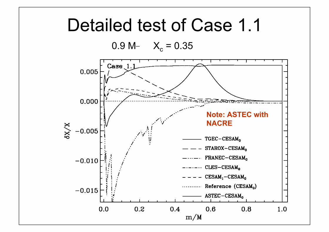
Detailed test of Case 1.10.9 M¯ Xc = 0.35

Note: ASTEC withNACRE

(3He evolution, τ3 = 107 years) –(3He equil.)

Note: early small convection core.

Case 1.1

0.9 M¯, Xc = 0.35

ASTEC (3He equilibrium) -CESAM δ X

Differences at fixed m

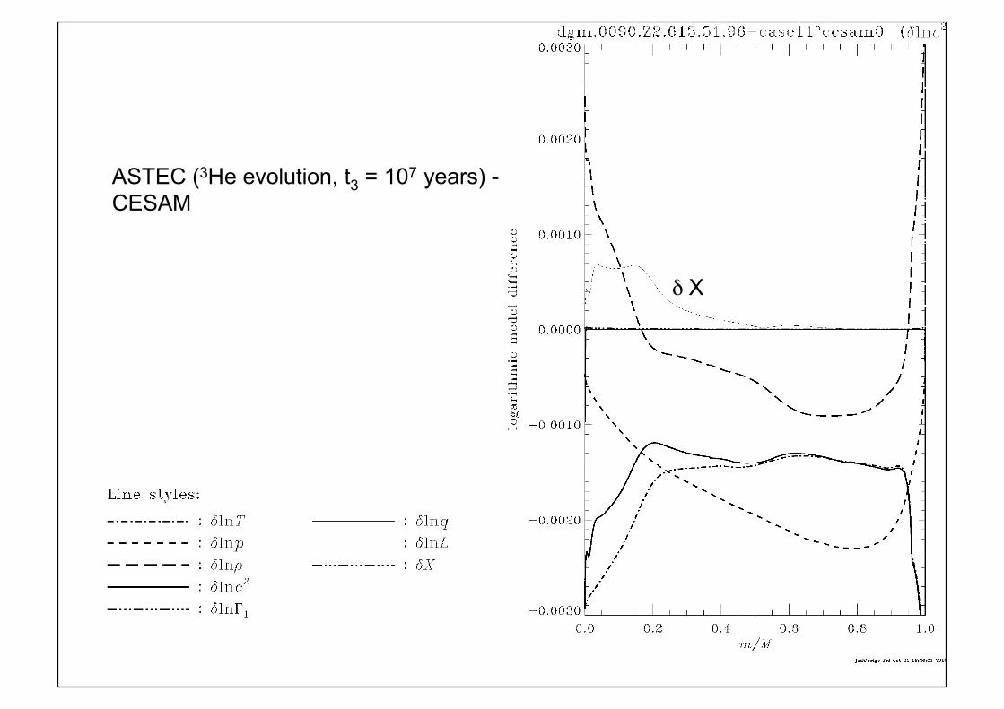
ASTEC (3He evolution, t3 = 107 years) -CESAM

δ X

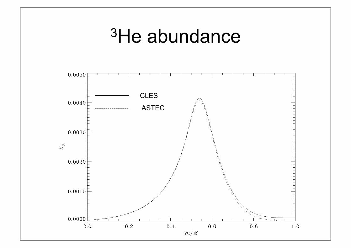
3He abundance

CLES

ASTEC

3He in equilibrium

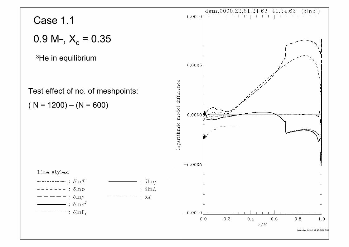
Case 1.1

0.9 M¯, Xc = 0.35

Test effect of no. of meshpoints:

( N = 1200) – (N = 600)

3He in equilibrium

Case 1.3

1.2 M¯, Mc = 0.1 M¯

Test effect of no. of meshpoints:

( N = 1200) – (N = 600)

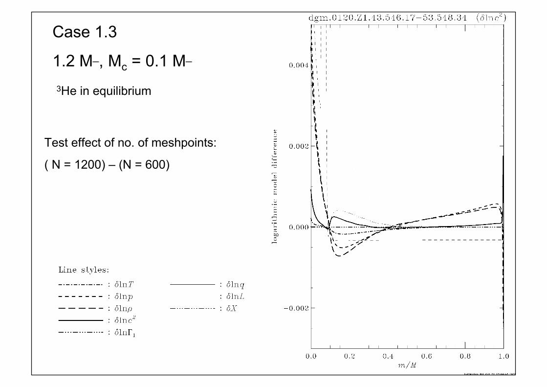
3He in equilibrium

Case 1.3

1.2 M¯, Mc = 0.1 M¯

Test effect of no. of meshpoints:

( N = 1200) – (N = 600)

3He in equilibrium

Case 1.1

0.9 M¯, Xc = 0.35

Test effect of no. timesteps:

( Nt = 24) – (Nt = 13)

(Δ ymax = 0.025) - (Δ ymax = 0.05)

3He in equilibrium

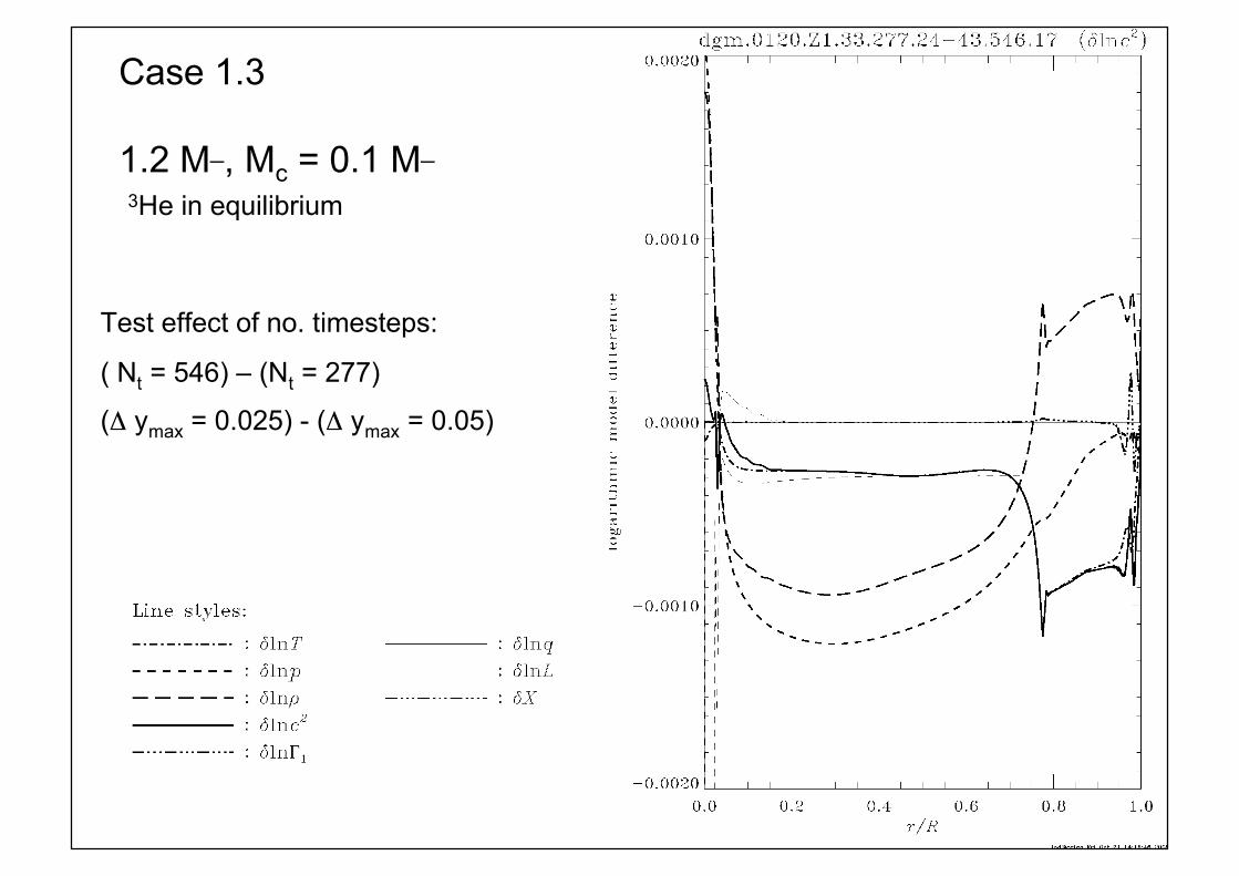
Case 1.3

1.2 M¯, Mc = 0.1 M¯

Test effect of no. timesteps:

( Nt = 546) – (Nt = 277)

(Δ ymax = 0.025) - (Δ ymax = 0.05)

Physics comparisons

Evaluate physics (EOS, opacity, energy-generationrate, rate of composition change, …, at fixed T, ρ, Xi

Examples: comparing CESAM and CLES withASTEC, showing, e.g.,

ln(κASTEC(ρCESAM, TCESAM, …)/κCESAM)

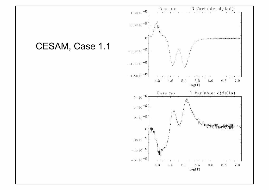
CESAM, Case 1.1

Note: consistency problems in OPAL.

See also Boothroyd & Sackman (2003;ApJ 583, 1004)

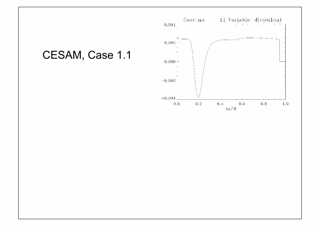
CESAM, Case 1.1

CESAM, Case 1.1

CESAM, Case 1.1

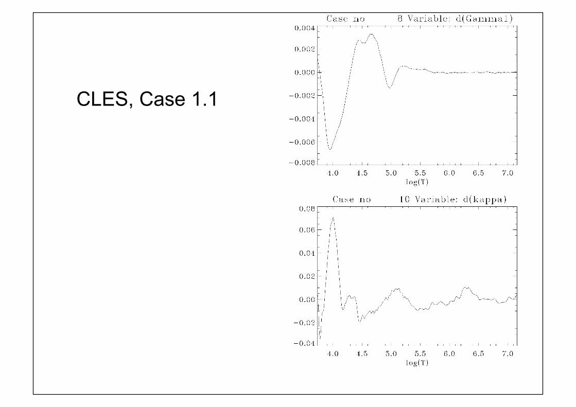
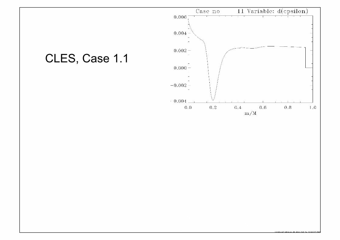
CLES, Case 1.1

CLES, Case 1.1

CLES, Case 1.1

CLES, Case 1.1