
Assumptions to the Annual Energy Outlook 2009
190
Report #:DOE/EIA-0554(2009) Release date: March 2009 Next release date: March 2010 Assumptions to the Annual Energy Outlook 2009
Transcript of Assumptions to the Annual Energy Outlook 2009

Report #:DOE/EIA-0554(2009)
Release date: March 2009
Next release date: March 2010
Assumptions to the Annual Energy Outlook 2009


1. Introduction . . . . . . . . . . . . . . . . . . . . . . . . . . . . . . . . . . . . . . . . . . 1
2. Macroeconomic Activity Module . . . . . . . . . . . . . . . . . . . . . . . . . . . . . . . 13
3. International Energy Module . . . . . . . . . . . . . . . . . . . . . . . . . . . . . . . . . 15
4. Residential Demand Module . . . . . . . . . . . . . . . . . . . . . . . . . . . . . . . . . 21
5. Commercial Demand Module . . . . . . . . . . . . . . . . . . . . . . . . . . . . . . . . 31
6. Industrial Demand Module . . . . . . . . . . . . . . . . . . . . . . . . . . . . . . . . . . 43
7. Transportation Demand Module . . . . . . . . . . . . . . . . . . . . . . . . . . . . . . . 59
8. Electricity Market Module . . . . . . . . . . . . . . . . . . . . . . . . . . . . . . . . . . 87
9. Oil and Gas Supply Module. . . . . . . . . . . . . . . . . . . . . . . . . . . . . . . . . 107
10. Natural Gas Transmission and Distribution Module . . . . . . . . . . . . . . . . . . . . 123
11. Petroleum Market Module . . . . . . . . . . . . . . . . . . . . . . . . . . . . . . . . . 131
12. Coal Market Module . . . . . . . . . . . . . . . . . . . . . . . . . . . . . . . . . . . . 143
13. Renewable Fuels Module . . . . . . . . . . . . . . . . . . . . . . . . . . . . . . . . . 155
Appendix A: Handling of Federal and Selected State Legislationand Regulation In the Annual Energy Outlook . . . . . . . . . . . . . . . . . . . . . . . . 169
Contents


IntroductionThis report presents the major assumptions of the National Energy Modeling System (NEMS) used togenerate the projections in the Annual Energy Outlook 20091 (AEO2009), including general features of themodel structure, assumptions concerning energy markets, and the key input data and parameters that arethe most significant in formulating the model results. Detailed documentation of the modeling system isavailable in a series of documentation reports.2
The National Energy Modeling System
The projections in the AEO2009 were produced with the NEMS, which is developed and maintained by theOffice of Integrated Analysis and Forecasting of the Energy Information Administration (EIA) to provideprojections of domestic energy-economy markets in the long term and perform policy analyses requested bydecisionmakers in the White House, U.S. Congress, offices within the Department of Energy, including DOEProgram Offices, and other government agencies. The Annual Energy Outlook (AEO) projections are alsoused by analysts and planners in other government agencies and outside organizations.
The time horizon of NEMS is approximately 25 years, the period in which the structure of the economy andthe nature of energy markets are sufficiently understood that it is possible to represent considerablestructural and regional detail. Because of the diverse nature of energy supply, demand, and conversion inthe United States, NEMS supports regional modeling and analysis in order to represent the regionaldifferences in energy markets, to provide policy impacts at the regional level, and to portray transportationflows. The level of regional detail for the end-use demand modules is the nine Census divisions. Otherregional structures include production and consumption regions specific to oil, natural gas, and coal supplyand distribution, the North American Electric Reliability Council (NERC) regions and subregions forelectricity, and the Petroleum Administration for Defense Districts (PADDs) for refineries. Maps illustratingthe regional formats used in each module are included in this report. Only selected regional results arepresented in the AEO2009, which predominately focuses on the national results. Complete regional anddetailed results are available on the EIA Forecasts and Analyses Home Page (http://www.eia.doe.gov/oiaf/aeo/index.html)
For each fuel and consuming sector, NEMS balances the energy supply and demand, accounting for theeconomic competition between the various energy fuels and sources. NEMS is organized and implementedas a modular system (Figure 1). The modules represent each of the fuel supply markets, conversion sectors,and end-use consumption sectors of the energy system. NEMS also includes a macroeconomic and aninternational module. The primary flows of information between each of these modules are the deliveredprices of energy to the end user and the quantities consumed by product, region, and sector. The deliveredprices of fuel encompass all the activities necessary to produce, import, and transport fuels to the end user.The information flows also include other data such as economic activity, domestic production, andinternational petroleum supply availability.
The integrating module of NEMS controls the execution of each of the component modules. To facilitatemodularity, the components do not pass information to each other directly but communicate through acentral data storage location. This modular design provides the capability to execute modules individually,thus allowing decentralized development of the system and independent analysis and testing of individualmodules. This modularity allows use of the methodology and level of detail most appropriate for each energysector. NEMS solves by calling each supply, conversion, and end-use demand module in sequence until thedelivered prices of energy and the quantities demanded have converged within tolerance, thus achieving aneconomic equilibrium of supply and demand in the consuming sectors. Solution is reached annually throughthe projection horizon. Other variables are also evaluated for convergence such as petroleum productimports, crude oil imports, and several macroeconomic indicators.
Energy Information Administration/Assumptions to the Annual Energy Outlook 2009 1
Report #:DOE/EIA-0554(2009)
Release date: March 2009
Next release date: March 2010

Each NEMS component also represents the impact and cost of Federal legislation and regulation that affect thesector and reports key emissions. NEMS generally reflects all current legislation and regulation that are definedsufficiently to be modeled as of November 5, 2008, such as the Energy Improvement and Extension Act of 2008(EIEA2008), the biofuel provisions of the Food, Conservation, and Energy Act of 2008, the EnergyIndependence and Security Act of 2007 (EISA2007), the Energy Policy Act of 2005, Military ConstructionAppropriations Act of 2005, the Working Families Tax Relief Act of 2004, and the America Jobs Creation Actof 2004, and the costs of compliance with regulations such as new stationary diesel regulations issued by theU.S. Environmental Protection Agency (EPA) on July 11, 2006, which limit emissions of nitrogen oxides,particulate matter, sulfur dioxide, carbon monoxide, and hydrocarbons to the same levels required by theEPA’s nonroad diesel engine regulations and court decisions that impact regulations such as the recentdecisions by the D.C. Circuit of the U.S. Court of Appeals on February 8, 2008, to vacate the Clean AirMercury Rule (CAMR) and on July 11, 2008, to vacate the Clean Air Interstate Rule (CAIR).3 The NEMScomponents also reflect selected State legislation and regulations where implementing regulations are clearsuch as the October 2008 decision by the California Air Resources Board (CARB) on California’s LowCarbon Fuel Standard (LCFS) requiring a 10-percent ethanol blend, by volume, in gasoline,. However, thepotential impacts of pending or proposed legislation, regulations, and standards—or of sections oflegislation that have been enacted but that require implementing regulations or appropriation of funds thatare not provided or specified in the legislation itself—are not reflected in NEMS. A list of the specific Federaland selected State legislation and regulations included in the AEO, including how they are incorporated, is providedin Appendix A..
Component Modules
The component modules of NEMS represent the individual supply, demand, and conversion sectors ofdomestic energy markets and also include international and macroeconomic modules. In general, themodules interact through values representing the prices of energy delivered to the consuming sectors andthe quantities of end-use energy consumption. This section provides brief summaries of each of themodules.
Macroeconomic Activity Module
The Macroeconomic Activity Module (MAM) provides a set of macroeconomic drivers to the energymodules, and there is a macroeconomic feedback mechanism within NEMS. Key macroeconomic variables
2 Energy Information Administration/Assumptions to the Annual Energy Outlook 2009
Oil and GasSupply Module
Natural GasTransmission
and DistributionModule
Coal MarketModule
RenewableFuels Module
Supply
ResidentialDemand Module
CommercialDemandModule
TransportationDemand Module
IndustrialDemand Module
Demand
ElectricityMarketModule
PetroleumMarketModule
Conversion
MacroeconomicActivityModule
InternationalEnergyModule
Integrating
Module
Figure 1. National Energy Modeling System
Source: Energy Information Administration, Office of Integrated Analysis and Forecasting.

used in the energy modules include gross domestic product (GDP), disposable income, value of industrialshipments, new housing starts, new light-duty vehicle sales, interest rates, and employment. The MAMmodule uses the following models from Global Insight, Inc.: Macroeconomic Model of the U.S. Economy,National Industry Model, and National Employment Model. In addition, EIA has constructed a RegionalEconomic and Industry Model to project regional economic drivers and a Commercial Floorspace Model toproject 13 floorspace types in 9 Census divisions. The accounting framework for industrial value ofshipments uses the North American Industry Classification System (NAICS)..
International ModuleThe International Module represents the response of world oil markets (supply and demand) to assumedworld oil prices. The results/outputs of the module are a set of crude oil and product supply curves that areavailable to U.S. markets for each case/scenario analyzed. The petroleum import supply curves are madeavailable to U.S. markets through the Petroleum Market Module (PMM) of NEMS in the form of 5 categoriesof imported crude oil and 17 international petroleum products, including supply curves for oxygenates andunfinished oils. The supply-curve calculations are based on historical market data and a world oilsupply/demand balance, which is developed from reduced-form models of international liquids supply anddemand, current investment trends in exploration and development, and long-term resource economics for221 countries/territories. The oil production estimates include both conventional and unconventional supplyrecovery technologies.
Residential and Commercial Demand ModulesThe Residential Demand Module projects energy consumption in the residential sector by housing type andend use, based on delivered energy prices, the menu of equipment available, the availability of renewablesources of energy, and housing starts. The Commercial Demand Module projects energy consumption inthe commercial sector by building type and nonbuilding uses of energy and by category of end use, based ondelivered prices of energy, availability of renewable sources of energy, and macroeconomic variablesrepresenting interest rates and floorspace construction.
Both modules estimate the equipment stock for the major end-use services, incorporating assessments ofadvanced technologies, including representations of renewable energy technologies, and the effects of bothbuilding shell and appliance standards, including the recently enacted provisions of the EISA2007. TheCommercial Demand Module incorporates combined heat and power (CHP) technology. The modules alsoinclude projections of distributed generation. Both modules incorporate changes to “normal” heating andcooling degree-days by Census division, based on a 10-year average and on State-level populationprojections. The Residential Demand Module projects an increase in the average square footage of bothnew construction and existing structures, based on trends in the size of new construction and the remodelingof existing homes.
Industrial Demand ModuleThe Industrial Demand Module projects the consumption of energy for heat and power and for feedstocksand raw materials in each of 21 industries, subject to the delivered prices of energy and macroeconomicvariables representing employment and the value of shipments for each industry. As noted in the descriptionof the MAM, the value of shipments is based on NAICS. The industries are classified into threegroups—energy-intensive manufacturing, non-energy-intensive manufacturing, and nonmanufacturing. Ofthe eight energy-intensive industries, seven are modeled in the Industrial Demand Module, with componentsfor boiler/steam/cogeneration, buildings, and process/ assembly use of energy. Bulk chemicals are furtherdisaggregated to organic, inorganic, resins, and agricultural chemicals. A generalized representation ofcogeneration and a recycling component are also included. The use of energy for petroleum refining ismodeled in the PMM, and the projected consumption is included in the industrial totals.
Transportation Demand ModuleThe Transportation Demand Module projects consumption of fuels in the transportation sector, includingpetroleum products, electricity, methanol, ethanol, compressed natural gas, and hydrogen, by transportationmode, vehicle vintage, and size class, subject to delivered prices of energy fuels and macroeconomicvariables representing disposable personal income, GDP, population, interest rates, and industrial
Energy Information Administration/Assumptions to the Annual Energy Outlook 2009 3

shipments. Fleet vehicles are represented separately to allow analysis of the Energy Policy Act of 1992(EPACT1992) and other legislation and legislative proposals. The transportation demand module alsoincludes a component to assess the penetration of alternative-fuel vehicles. EPACT2005 and EIEA2008 arereflected in the assessment of the impact of tax credits on the purchase of hybrid gas-electric,alternative-fuel, and fuel-cell vehicles. The corporate average fuel economy and biofuel representation in themodule reflect standards proposed by the National Highway Traffic Safety Administration and provisions inEISA2007.
The air transportation component explicitly represents air travel in domestic and foreign markets andincludes the industry practice of parking aircraft in both domestic and international markets to reduceoperating costs, as well as the movement of aging aircraft from passenger to cargo markets4. For passengertravel and air freight shipments, the model represents regional fuel use in regional, narrow-body, andwide-body aircraft. An infrastructure constraint is also modeled and can potentially limit overall growth inpassenger and freight air travel to levels commensurate with industry-projected infrastructure expansionand capacity growth.
Electricity Market Module
The Electricity Market Module (EMM) represents generation, transmission, and pricing of electricity, subjectto delivered prices for coal, petroleum products, natural gas, and biofuels; costs of generation by allgeneration plants, including capital costs and macroeconomic variables for costs of capital and domesticinvestment; environmental emissions laws and regulations; and electricity load shapes and demand. Thereare three primary submodules—capacity planning, fuel dispatching, and finance and pricing.
All specifically identified options promulgated by the EPA for compliance with the Clean Air Act Amendmentsof 1990 (CAAA90) are explicitly represented in the capacity expansion and dispatch decisions; those thathave not been promulgated (e.g., fine particulate proposals) are not incorporated. All financial incentives forpower generation expansion and dispatch specifically identified in EPACT2005 have been implemented.Several States, primarily in the Northeast, have recently enacted air emission regulations for carbon dioxide(CO2) that affect the electricity generation sector, and these regulations are represented in AEO2009.
Although Federal legislation restricting greenhouse gas (GHG) emissions are not currently in place,regulators and the investment community are beginning to push energy companies to invest in lessGHG-intensive technologies. This was captured in the AEO2009 reference case through a 3-percentagepoint increase in the cost of capital when evaluating investments in new coal-fired power plants withoutcarbon control and sequestration, and new coal-to-liquids plants.
Renewable Fuels Module
The Renewable Fuels Module (RFM) includes submodules representing renewable resource supply andtechnology input information for central-station, grid-connected electricity generation technologies, includingconventional hydroelectricity, biomass (wood, energy crops, and biomass co-firing), geothermal, landfill gas,solar thermal electricity, solar photovoltaics (PV), and wind energy. The RFM contains renewable resourcesupply estimates representing the regional opportunities for renewable energy development. Investment taxcredits for renewable fuels are incorporated, as currently enacted. This includes a permanent 10-percent taxcredit for business investment in solar energy (thermal non-power uses as well as power uses) andgeothermal power (only available to those projects not accepting the production tax credit). In addition, themodule reflects the increase in the tax credit to 30 percent for solar energy systems installed before January1, 2017 and the extension of the credit to individual homeowners under EIEA2008.
Production tax credits for wind, geothermal, landfill gas, and some types of hydroelectric and biomass-fueledplants are also represented. They provide a tax credit of up to 2.0 cents per kilowatthour for electricityproduced in the first 10 years of plant operation. For AEO2009, new plants coming on line before January 1,2010, are eligible to receive the credit. AEO2009 also accounts for new renewable energy capacity resultingfrom State renewable portfolio standard programs, mandates, and goals, as described in Assumptions to theAnnual Energy Outlook 2009 5.
4 Energy Information Administration/Assumptions to the Annual Energy Outlook 2009

Oil and Gas Supply ModuleThe Oil and Gas Supply Module (OGSM) represents domestic crude oil and natural gas supply within anintegrated framework that captures the interrelationships among the various sources of supply: onshore,offshore, and Alaska by both conventional and unconventional techniques, including natural gas recoveryfrom coalbeds and low-permeability formations of sandstone and shale. The framework analyzes cash flowand profitability to compute investment and drilling for each of the supply sources, based on the prices forcrude oil and natural gas, the domestic recoverable resource base, and the state of technology. Oil and gasproduction functions are computed for 12 supply regions, including 3 offshore and 3 Alaskan regions. Themodule also represents foreign sources of natural gas, including pipeline imports and exports to Canada andMexico, and liquefied natural gas (LNG) imports and exports.
Crude oil production quantities are input to the PMM in NEMS for conversion and blending into refinedpetroleum products. Supply curves for natural gas are input to the Natural Gas Transmission andDistribution Module (NGTDM) for use in determining natural gas prices and quantities. International LNGsupply sources and options for construction of new regasification terminals in Canada, Mexico, and theUnited States as well as expansions of existing U.S. regasification terminals are represented, based on theprojected regional costs associated with international natural gas supply, liquefaction, transportation, andregasification and world natural gas market conditions.
Natural Gas Transmission and Distribution ModuleThe NGTDM represents the transmission, distribution, and pricing of natural gas, subject to end-usedemand for natural gas and the availability of domestic natural gas and natural gas traded on theinternational market. The module tracks the flows of natural gas and determines the associated capacityexpansion requirements in an aggregate pipeline network, connecting the domestic and foreign supplyregions with 12 U.S. demand regions. The flow of natural gas is determined for both a peak and off-peakperiod in the year. Key components of pipeline and distributor tariffs are included in separate pricingalgorithms. The module also represents foreign sources of natural gas, including pipeline imports andexports to Canada and Mexico, and imports and exports LNG.
Petroleum Market ModuleThe PMM projects prices of petroleum products, crude oil and product import activity, and domestic refineryoperations (including fuel consumption), subject to the demand for petroleum products, the availability andprice of imported petroleum, and the domestic production of crude oil, natural gas liquids, and biofuels(ethanol, biodiesel, and biomass-to-liquids (BTL)). The module represents refining activities in the fivePADDs, as well as a less detailed representation of refining activities in the rest of the world. It explicitlymodels the requirements of EISA2007 and CAAA90 and the costs of automotive fuels, such as conventionaland reformulated gasoline, and includes the production of biofuels for blending in gasoline and diesel.
AEO2009 represents regulations that limit the sulfur content of all nonroad and locomotive/marine diesel to15 parts per million (ppm) by mid-2012. The module also reflects the new renewable fuels standard (RFS) inEISA2007 that requires the use of 36 billion gallons per year of biofuels by 2022 if achievable, with cornethanol limited to 15 billion gallons per year. Demand growth and regulatory changes necessitate capacityexpansion for refinery processing units. U.S. end-use prices are based on the marginal costs of production,plus markups representing the costs of product marketing, importing, transportation and distribution as wellas applicable State and Federal taxes6. Refinery capacity expansion at existing sites is permitted in eachE85, a blend of up to 85 percent ethanol by volume. In the AEO2009, the level of allowable non-E85 ethanolblending in California was raised from 5.7 percent to 10 percent in recent regulatory changes7 which haveset a framework for E10 emission standards. of the five refining regions modeled.
Fuel ethanol and biodiesel are included in the PMM, because they are commonly blended into petroleumproducts. The module allows ethanol blending into gasoline at 10 percent or less by volume (E10), as well asE85, a blend of up to 85 percent ethanol by volume. In the AEO2009, the level of allowable non-E85 ethanolblending in California was raised from 5.7 percent to 10 percent in recent regulatory changes8 which haveset a framework for E10 emission standards.
Energy Information Administration/Assumptions to the Annual Energy Outlook 2009 5

Both domestic and imported ethanol count toward the RFS. Domestic ethanol production is modeled fromtwo feedstocks: corn and cellulosic materials. Corn-based ethanol plants are numerous (more than 150 arenow in operation, possessing a total production capacity of more than 10 billion gallons annually) and arebased on a well-known technology that converts sugar into ethanol. Ethanol from cellulosic sources is a newtechnology with no pilot plants in operation; however, DOE awarded grants (up to $385 million) in 2007 toconstruct capacity totaling 147 million gallons per year, which AEO2009 assumes will be operational startingin 2012. Imported ethanol may be produced from cane sugar or bagasse, the cellulosic byproduct of sugarmilling. The sources of ethanol are modeled to compete on an economic basis and to meet the EISA2007renewable fuels mandate.
Coal Market Module
The Coal Market Module (CMM) simulates mining, transportation, and pricing of coal, subject to end-usedemand for coal differentiated by heat and sulfur content. U.S. coal production is represented in the CMM by40 separate supply curves—differentiated by region, mine type, coal rank, and sulfur content. The coalsupply curves include a response to capacity utilization of mines, mining capacity, labor productivity, andfactor input costs (mining equipment, mining labor, and fuel requirements), and other mine supply costs.Projections of U.S. coal distribution are determined by minimizing the cost of coal supplied, given coaldemands by demand region and sector, environmental restrictions, and accounting for minemouth prices,transportation rates, and coal supply contracts. Over the projection horizon, coal transportation rates in theCMM are projected to vary in response to changes in railroad investment and market share (for westernrates only).
The CMM produces projections of U.S. steam and metallurgical coal exports and imports, in the context ofworld coal trade. The CMM determines the pattern of world coal trade flows that minimizes the productionand transportation costs of meeting a specified set of regional world coal import demands, subject toconstraints on export capacities and trade flows. The international coal market component of the modulecomputes trade in 3 types of coal for 17 export and 20 import regions. U.S. coal production and distributionare computed for 14 supply and 14 demand regions.
Cases for the Annual Energy Outlook 2009
In preparing projections for the AEO2009, EIA evaluated a wide range of trends and issues that could havemajor implications for U.S. energy markets between now and 2030. Besides the reference case, theAEO2009 presents detailed results for four alternative cases that differ from each other due to fundamentalassumptions concerning the domestic economy and world oil market conditions. These alternative casesinclude the following:
• Economic Growth - In the reference case, real GDP grows at an average annual rate of 2.5 percentfrom 2007 through 2030, supported by a 2.0 percent per year growth in productivity in nonfarmbusiness and a 0.9 percent per year growth in nonfarm employment. In the high economic growthcase, real GDP is projected to increase by 3.0 percent per year, with productivity and nonfarmemployment growing at 2.4 percent and 1.3 percent per year, respectively. In the low economicgrowth case, the average annual growth in GDP, productivity and nonfarm employment is 1.8, 1.5and 0.5 percent, respectively.
• Price Cases – For purposes of the AEO2009, the world oil price is defined by the price of light,low-sulfur crude oil delivered in Cushing, Oklahoma. In the reference case, world oil prices increasequickly after the recession ends, reaching $110 per barrel in 2015 ($128 per barrel in nominal terms),as growth in world oil demand rebounds and investment in production capacity lags this expansion indemand. After 2015, real prices rise gradually as demand continues to grow and higher cost suppliesare brought to market. In 2030, the average real price of crude oil is $130 per barrel in 2007 dollars, orabout $189 per barrel in nominal dollars. The reference case represents EIA’s current judgmentabout the most likely behavior of key Organization of Petroleum Exporting Country (OPEC) membersin the mid term. In the projection, OPEC countries increase production at a rate that keeps theirmarket share of world liquids production at approximately 41 percent through 2030. The low and highprice cases define a wide range of potential price paths, which in 2030 span from $50 to $200 perbarrel in real dollars. These cases reflect differences in the assumptions about access to energy
6 Energy Information Administration/Assumptions to the Annual Energy Outlook 2009

resources, production costs, and changes in OPEC behavior. The low price case assumes greatereconomic access to world crude oil resources that are less expensive to produce and a future marketwhere all oil and natural gas production becomes more competitive and plentiful than the referencecase. The high price case assumes that the production of conventional crude oil will cost more than inthe reference case and will be limited due to increased restrictions on economic access to non-OPECresources and OPEC decisions to further limit its production.
In addition to these four cases, and the reference case, 31 additional alternative cases presented in Table1.1 that explore the impact of changing key assumptions on individual sectors.
Many of the side cases were designed to examine the impacts of varying key assumptions for individualmodules or a subset of the NEMS modules, and thus the full market consequences, such as theconsumption or price impacts, are not captured. In a fully integrated run, the impacts would tend to narrowthe range of the differences from the reference case. For example, the best available technology side case inthe residential demand assumes that all future equipment purchases are made from a selection of the mostefficient technologies available in a particular year. In a fully integrated NEMS run, the lower resulting fuelconsumption would have the effect of lowering the market prices of those fuels with the concomitant impactof increasing economic growth, thus stimulating some additional consumption. The results of single model orpartially integrated cases should be considered the maximum range of the impacts that could occur with theassumptions defined for the case.
Energy Information Administration/Assumptions to the Annual Energy Outlook 2009 7
Case name Description Integrationmode
Reference Baseline economic growth (2.5 percent per year from 2007through 2030), world oil price, and technology assumptions.Complete projection tables in Appendix A.
Fully integrated
Low Economic Growth GDP grows at an average annual rate of 1.8 percent from 2007through 2030. Other energy market assumptions are the same asin the reference case. Partial projection tables in Appendix B.
Fully integrated
High Economic Growth GDP grows at an average annual rate of 3.0 percent from 2007through 2030. Other energy market assumptions are the same asin the reference case. Partial projection tables in Appendix B.
Fully integrated
Low Oil Price More optimistic assumptions for economic access to non-OPECresources and the behavior of the OPEC than in the referencecase. World light, sweet crude oil prices are $50 per barrel in2030, compared with $130 per barrel in the reference case (2007dollars). Other assumptions are the same as in the referencecase. Partial projection tables in Appendix C.
Fully integrated
High Oil Price More pessimistic assumptions for economic access to non-OPECresources and OPEC behavior than in the reference case. Worldlight, sweet crude oil prices are about $200 per barrel (2007dollars) in 2030. Other assumptions are the same as in thereference case. Partial projection tables in Appendix C..
Fully integrated
Residential:2009 Technology
Future equipment purchases based on equipment available in2009. Existing building shell efficiencies fixed at 2009 levels.Partial projection tables in Appendix D.
With commercial
Residential: HighTechnology
Earlier availability, lower costs, and higher efficiencies assumedfor more advanced equipment. Building shell efficiencies for newconstruction meet ENERGY STAR requirements after 2016.Partial projection tables in Appendix D.
With commercial
Residential: BestAvailable Technology
Future equipment purchases and new building shells based onmost efficient technologies available by fuel. Building shellefficiencies for new construction meet the criteria for most efficientcomponents after 2009. Partial projection tables in Appendix D.
With commercial
Commercial:2009 Technology
Future equipment purchases based on equipment available in2009. Building shell efficiencies fixed at 2009 levels. Partialprojection tables in Appendix D.
With residential
Table 1.1. Summary of AEO2009 Cases

8 Energy Information Administration/Assumptions to the Annual Energy Outlook 2009
Case name Description Integrationmode
Commercial:HighTechnology
Earlier availability, lower costs, and higher efficienciesassumed for more advanced equipment. Building shellefficiencies for new and existing buildings increase by8.8 and 6.3 percent, respectively, from 2003 values by2030. Partial projection tables in Appendix D.
With residential
Commercial: BestAvailable Technology
Future equipment purchases based on most efficienttechnologies available by fuel. Building shell efficiencies fornew and existing buildings increase by 10.5 and 7.5 percent,respectively, from 2003 values by 2030. Partial projectiontables in Appendix D.
With residential
Industrial: 2009Technology
Efficiency of plant and equipment fixed at 2009 levels.Partial projection tables in Appendix D.
Standalone
Industrial:High Technology
Earlier availability, lower costs, and higher efficienciesassumed for more advanced equipment. Partial projectiontables in Appendix D.
Standalone
Transportation:Low Technology
Assumes advanced technologies are more costly and lessefficient then in reference case. Partial projection tables inAppendix D
Standalone
Transportation:High Technology
Assumes advanced technologies are less costly and moreefficient then in reference case. Partial projection tables inAppendix D.
Standalone
Electricity: Low Nuclear Cost New nuclear capacity assumed to have 25 percent lowercapital and operating costs in 2030 than in the referencecase. Partial projection tables in Appendix D.
Fully Integrated
Electricity: High Nuclear Cost Costs for new nuclear technology assumed not to improvefrom 2009 levels in the reference case. Existing nuclearplants are assumed to retire after 55 years. Partial projectiontables in Appendix D.
Fully Integrated
Electricity: Low FossilTechnology Cost
Capital and operating costs for all new fossil-fired generatingtechnologies improve by 25 percent in 2030 from referencecase values. Partial projection tables in Appendix D.
Fully Integrated
Electricity: High FossilTechnology Cost
Costs for new advanced fossil generating technologiesassumed not to improve over time from 2009. Partialprojection tables in Appendix D.
Fully Integrated
Renewable Fuels: HighRenewable TechnologyCost
New renewable generating technologies assumed not toimprove over time from 2009. Partial projection tables inAppendix D.
Fully integrated
Renewable Fuels: LowRenewable TechnologyCost
Levelized cost of energy for non-hydropower renewablegenerating technologies declines by 25 percent in 2030from reference case values. Partial projection tables inAppendix D.
Fully integrated
Renewable Fuels:Production Tax CreditExtension
PTC for certain renewable generation is assumed to beextended to projects constructed through2016.
Fully integrated
Oil and Gas:Rapid Technology
Cost, finding rate, and success rate parameters adjustedfor 50-percent more rapid improvement than in thereference case. Partial projection tables in Appendix D.
Fully integrated
Oil and Gas:Slow Technology
Cost, finding rate, and success rate parameters adjustedfor 50-percent slower improvement than in the referencecase. Partial projection tables in Appendix D.
Fully integrated
Oil and Gas: HighLNG Supply
LNG imports exogenously set to a factor times the referencecase levels from 2010 forward, with remaining assumptionsfrom the reference case. The factor starts at 1.0 in 2010 andincreases linearly to 5.0 by 2030. Partial projection tables inAppendix D.
Fully Integrated
Table 1.1. Summary of AEO2009 Cases (cont.)

Energy Information Administration/Assumptions to the Annual Energy Outlook 2009 9
Case name Description Integrationmode
Oil and Gas: LowLNG Supply
LNG imports held constant at 2009 levels, with remainingassumptions from the reference case. Partial projectiontables in Appendix D.
Fully Integrated
Oil and Gas: ANWR The Arctic National Wildlife Refuge (ANWR) in Alaskais opened to Federal oil and natural gas leasing, withremaining assumptions from the reference case. Partialprojection tables in Appendix D.
Fully Integrated
Oil and Gas:No Alaska Pipeline
A natural gas pipeline from the North Slope of Alaskato the Lower 48 States is assumed not to be built duringthe projection period.
Fully Integrated
Coal: Low Coal Cost Productivity growth rates for coal mining are assumedto be higher than in the reference case, and coal miningwages, mine equipment, and coal transportation ratesare assumed to be lower. Partial projection tables inAppendix D.
Fully Integrated
Coal: High Coal Cost Productivity growth rates for coal mining are assumed to belower than in the reference case, and coal mining wages,mine equipment, and coal transportation rates are assumedto be higher. Partial projection tables in Appendix D.
Fully integrated
Integrated 2009Technology
Combination of the residential, commercial, and industrial2009 technology cases; and the electricity high fossiltechnology cost, high renewable technology cost, and highnuclear cost cases. Partial projection tables in Appendix D
Fully integrated
Integrated HighTechnology
Combination of the residential, commercial, industrial, andtransportation high technology cases; and the electricitylow fossil technology cost, low renewable technology cost,and low nuclear cost cases. Partial projection tables inAppendix D.
Fully integrated
Electricity: Frozen PlantCosts
Base overnight costs for all new electric generatingtechnologies are assumed to be frozen at 2012 levels.Cost decreases due to learning still occur, but no declinesin costs due to commodity price changes are assumed.
Fully Integrated
Electricity: High PlantCapital Costs
Base overnight costs for all new electric generatingtechnologies are assumed to continue increasing through-out the projection, reaching 25 percent above 2012 costsin 2030. Cost decreases due to learning can still occur andmay partially offset these increases.
Fully Integrated
Electricity: Falling PlantCapital Costs
Base overnight costs for all new electric generatingtechnologies are assumed to fall more rapidly than in thereference case, reaching 25 percent below the referencecase costs in 2030.
Fully Integrated
No GHG Expectations Assumes that a greenhouse gas emission reduction policyis not enacted and markets do not alter their investmentdecisions in anticipation of such a policy.
Fully Integrated
Cap and Trade Assumes a greenhouse gas emission reduction policysimilar to that proposed in S.2191, the Lieberman-WarnerClimate Security Act of 2007 is implemented
Fully Integrated
No 2008 Tax Legislation Removes EIEA2008 tax legislation from reference case. Fully Integrated
Table 1.1. Summary of AEO2009 Cases (cont.)
Carbon Dioxide Emissions
Carbon dioxide emissions from energy use are dependent on the carbon content of the fossil fuel, thefraction of the fuel consumed in combustion, and the consumption of that fuel. The product of the carboncontent at full combustion and the combustion fraction yields an adjusted carbon emission factor for eachfossil fuel. The emissions factors are expressed in millions of metric tons carbon dioxide emitted perquadrillion Btu of energy use, or equivalently, in kilograms carbon dioxide per million Btu. The adjustedemissions factors are multiplied by the energy consumption of the fossil fuel to arrive at the carbon dioxideemissions projections.
For fuel uses of energy, the combustion fractions are assumed to be 1.00 in keeping with internationalconventions.9 Previously, a small fraction of the carbon content of the fuel was assumed to remainunoxidized. The carbon dioxide in nonfuel use of energy, such as for asphalt and petrochemical feedstocks,is assumed to be sequestered in the product and not released to the atmosphere. For energy categories thatare mixes of fuel and nonfuel uses, the combustion fractions are based on the proportion of fuel use. Anycarbon dioxide emitted by biogenic renewable sources, such as biomass and alcohols, is consideredbalanced by the carbon dioxide sequestration that occurred in its creation. Therefore, following convention,net emissions of carbon dioxide from biogenic renewable sources are taken as zero, and no emissioncoefficient is reported. In calculating carbon dioxide emissions for motor gasoline, the direct emissions fromrenewable blending stock (ethanol) is omitted. Similarly, direct emissions from biodiesel are omitted fromreported carbon dioxide emissions. Table 1.2 presents the assumed carbon dioxide coefficients at fullcombustion, the combustion fractions, and the adjusted carbon dioxide emission factors used for AEO2009.
10 Energy Information Administration/Assumptions to the Annual Energy Outlook 2009

Energy Information Administration/Assumptions to the Annual Energy Outlook 2009 11
Fuel Type
Carbon Dioxide Coefficient
at FullCombustion
CombustionFraction
AdjustedEmissions
FactorPetroleum
Motor Gasoline (net of ethanol) 70.88 1.000 70.88
Liquefied Petroleum Gas
Used as Fuel 63.00 1.000 63.00
Used as Feedstock 61.44 0.200 12.29
Jet Fuel 70.88 1.000 70.88
Distillate Fuel (net of biodiesel) 73.15 1.000 73.15
Residual Fuel 78.80 1.000 78.80
Asphalt and Road Oil 75.61 0.000 0.00
Lubricants 74.21 0.500 37.11
Petrochemical Feedstocks 69.85 0.386 26.93
Kerosene 72.31 1.000 72.31
Petroleum Coke 102.12 0.782 79.87
Petroleum Still Gas 64.20 1.000 64.20
Other Industrial 74.54 1.000 74.54
Coal
Residential and Commercial 95.35 1.000 95.35
Metallurgical 93.71 1.000 93.71
Coke 114.14 1.000 114.14
Industrial Other 93.98 1.000 93.98
Electric Utility1 94.70 1.000 94.70
Natural Gas
Used as Fuel 53.06 1.000 53.06
Used as Feedstocks 53.06 0.523 27.73
Table 1.2. Carbon Dioxide Emission Factors (million metric tons carbon dioxide equivalent per quadrillion Btu)
1Emission factors for coal used for electricity generation are specified by coal supply region and types of coal, so the average carbon dioxide contentsfor coal varies throughout the projection. The 2007 average is 94.70.
Source: Energy Information Administration, Emissions of Greenhouse Gases in the United States 2007, DOE/EIA-0573(2007), (Washington, DC,December 2008).

[1] Energy Information Administration, Annual Energy Outlook 2009 (AEO2009), DOE/EIA-0383(2009),(Washington, DC, February 2009).
[2] NEMS documentation reports are available on the EIA Homepage (http://tonto.eia.doe.gov/reports/reports_kindD.asp?type=model documentation).
[3] On December 23, 2008, after the November 5 cutoff date for inclusion of changes in Federal and Statelaws and regulations in AEO2009, the United States Court of Appeals for the District of Columbia issued anew ruling that remanded but did not vacate CAIR, noting that "Allowing CAIR to remain in effect until it isreplaced by a rule consistent with our opinion would at least temporarily preserve the environmental values."Source: United States Court of Appeals for the District of Columbia Circuit, No. 05-1244, web sitewww.epa.gov/airmarkets/progsregs/cair/docs/CAIRRemandOrder.pdf. This change allows the EPA tomodify CAIR to address the objections raised by the Court in its earlier decision while leaving the rule inplace. The change is not reflected in AEO2009.
[4] Jet Information Services, Inc., World Jet Inventory Year-End 2006 (Utica, NY, March 2007); and personalcommunication from Stuart Miller (Jet Information Services).
[5] Energy Information Administration, Assumptions to the Annual Energy Outlook 2009, DOE/EIA-0554(2009) (Washington, DC, February 2009), web site www.eia.doe.gov/oiaf/aeo/assumption
[6] For gasoline blended with ethanol, the tax credit of 51 cents (nominal) per gallon of ethanol is assumed tobe available for 2008. However, this tax credit is reduced to 45 cents as mandated by the “Food,Conservation, and Energy Act of 2008” (the “Farm Bill”) starting in 2009 (the year after the annual U.S.ethanol consumption surpasses 7.5 billion gallons); the tax credit is set to expire after 2010. In addition,modeling updates include the Farm Bill’s mandated extension of the 54 cent/gallon import tariff to Dec. 31,2010. Finally, again in accordance with the Farm Bill, a new cellulosic producer’s tax credit of $1.01/gallon isimplemented in the model (valid through 2012); however, this tax credit is reduced by the aforementionedblender’s tax credit amount. Thus, in 2009 and 2010, the cellulosic producer’s tax credit is modeled as $1.01- $0.45 = $0.56/gallon, and in 2011 and 2012 it is $1.01/gallon. http://www.arb.ca.gov/regact/2007/carfg07/carfg07.htm.
[7] Energy Information Administration, Assumptions to the Annual Energy Outlook 2009, DOE/EIA-0554(2009) (Washington, DC, February 2009), web site www.eia.doe.gov/oiaf/aeo/assumption.
[8] Energy Information Administration, Assumptions to the Annual Energy Outlook 2009, DOE/EIA-0554(2009) (Washington, DC, February 2009), web site www.eia.doe.gov/oiaf/aeo/assumption
[9] The Intergovernmental Panel on Climate Change 2006, 2006 IPCC Guidelines For National GreenhouseGas Inventories, prepared by the National Greenhouse Gas Inventories Program, published: IGES, Japan,2006.
12 Energy Information Administration/Assumptions to the Annual Energy Outlook 2009
Notes and Sources

Macroeconomic Activity ModuleThe Macroeconomic Activity Module (MAM) represents the interaction between the U.S. economy as awhole and energy markets. The rate of growth of the economy, measured by the growth in grossdomestic product (GDP) is a key determinant of the growth in demand for energy. Associated economicfactors, such as interest rates and disposable income, strongly influence various elements of the supply anddemand for energy. At the same time, reactions to energy markets by the aggregate economy, such as aslowdown in economic growth resulting from increasing energy prices, are also reflected in this module. Adetailed description of the MAM is provided in the EIA publication, Model Documentation Report:Macroeconomic Activity Module (MAM) of the National Energy Modeling System, DOE/EIA-M065(2008),(Washington, DC, January 2008).
Key Assumptions
The output of the U.S. economy, measured by GDP, is expected to increase by 2.5 percent between 2007and 2030 in the reference case. Two key factors help explain the growth in GDP: the growth rate of nonfarmemployment and the rate of productivity change associated with employment. As Table 2.1 indicates, realGDP growth slows during the first three years of the forecast, reflecting the current economic recession,shows higher growth for the first ten years as the economy recovers, and then returns to its long-run growthpath. In the reference case, real GPD grows by 0.7 percent for the first three years, 2.8 percent for therecovery period and 2.6 percent for the final ten years. Both the high and low macroeconomic growth casesshow similar patterns of early lower growth, recovery and settling back into their respective long-run growthtrends. In the near term from 2007 through 2010, the growth in nonfarm employment is low at -0.4 percentcompared with 2.4 percent in the second half of the 1990s, while the economy is expected to experienceproductivity growth of 1.8 percent. Over the projection period, nonfarm employment is expected to grow by0.9 percent per year. Nonfarm employment, a measure of demand for nonfarm labor, is generally morevolatile than the labor force, a measure of labor supply. The latter depends upon the pro jec t ion ofpopulation and labor force participation rate. The Census Bureau’s middle series population projection isused as a basis for population growth for the AEO2009. Total population is expected to grow by 0.9percent per year between 2007 and 2030, and the share of population over 65 is expected to increase overtime. However, the share of the labor force in the population over 65 is also projected to increase in theprojection period.
Energy Information Administration/Assumptions to the Annual Energy Outlook 2009 13
Assumptions 2007-2010 2010-2020 2020-2030 2007-2010GDP (Billion Chain-Weighted $2000)
High Growth 1.7 3.3 3.2 3.0
Reference 0.7 2.8 2.6 2.5
Low Growth -0.2 2.3 1.9 1.8
Nonfarm Employment
High Growth 0.8 1.5 1.2 1.3
Reference -0.4 1.2 1.0 0.9
Low Growth -1.6 0.8 0.8 0.5
Productivity
High Growth 2.3 2.3 2.5 2.4
Reference 1.8 1.9 2.1 2.0
Low Growth 1.5 1.4 1.5 1.5
Table 2.1. Growth in Gross Domestic Product, Nonfarm Employmemt and Productivity(Percent per Year)
Source: Energy Information Administration, AEO2009 National Energy Modeling System runs: AEO2009.d120908a;LM2009.d120908a; and hm2009.d120908a.
Report #:DOE/EIA-0554(2009)Release date: March 2009Next release date: March 2010

To achieve the reference case’s long-run 2.5 percent economic growth, there is an anticipated steadygrowth in labor productivity. The improvement in labor productivity reflects the positive effects of a growingcapital stock as well as technological change over time. Nonfarm labor productivity is expected to remainbetween 1.9 and 2.0 percent for the remainder of the projection period from 2007 through 2030. Businessfixed investment as a share of nominal GDP is expected to grow over the last 10 years of the projection. Theresulting growth in the capital stock and the technology base of that capital stock helps to sustain productivitygrowth of 2.0 percent from the 2007 to 2030.
To reflect the uncertainty in projection of economic growth, the AEO2009 uses high and low economicgrowth cases along with the reference case to project the possible impacts on energy markets. The higheconomic growth case incorporates higher population, labor force and productivity growth rates than thereference case. Due to the higher productivity gains, inflation and interest rates are lower compared to thereference case. Investment, disposable income, and industrial production are increased. Economic outputis projected to increase by 3.0 percent per year between 2007 and 2030. The low economic growth caseassumes lower population, labor force, and productivity gains, with resulting higher prices and interest ratesand lower industrial output growth. In the low economic growth case, economic output is expected toincrease by 1.8 percent per year over the projection horizon.
14 Energy Information Administration/Assumptions to the Annual Energy Outlook 2009

International Energy ModuleThe International Energy Module (IEM) performs two tasks in all NEMS runs. First, the module readsexogenously global and U.S.A. petroleum liquids supply and demand curves (1 curve per year; 2008-2030;approximated, isoelastic fit to previous NEMS results). These quantities are not modeled directly in NEMS.Previous versions of the IEM adjusted these quantities after reading in initial values. In an attempt to moreclosely integrate the AEO2009 with IEO2008 and the STEO some functionality was removed from IEM while a newalgorithm was implemented. Based on the difference between U.S. total petroleum liquids production(consumption) and the expected U.S. total liquids production (consumption) at the current WTI price, curves forglobal petroleum liquids consumption (production) were adjusted for each year. According to previousoperations, a new WTI price path was generated. An exogenous oil supply module, Generate World OilBalances (GWOB), was also used in IEM to provide annual regional (country) level production detail forconventional and unconventional liquids.
The second task of the IEM is to interact with the PMM module during runs to determine changes in the WTI price andthe supply prices of crude oils and petroleum products for import to the United States in response to changes in U.S.import requirements. As a result of the interaction with PMM, this module also determines new values for oilproduction in the world, along with a report for crude oil, light and heavy refined products imports by source.
Key Assumptions
The level of oil production by countries in the Organization of Petroleum Exporting Countries (OPEC) is a key factorinfluencing the world oil price projections incorporated into AEO2009. Non-OPEC production, worldwideregional economic growth rates and the associated regional demand for oil are additional factors affecting theworld oil price.
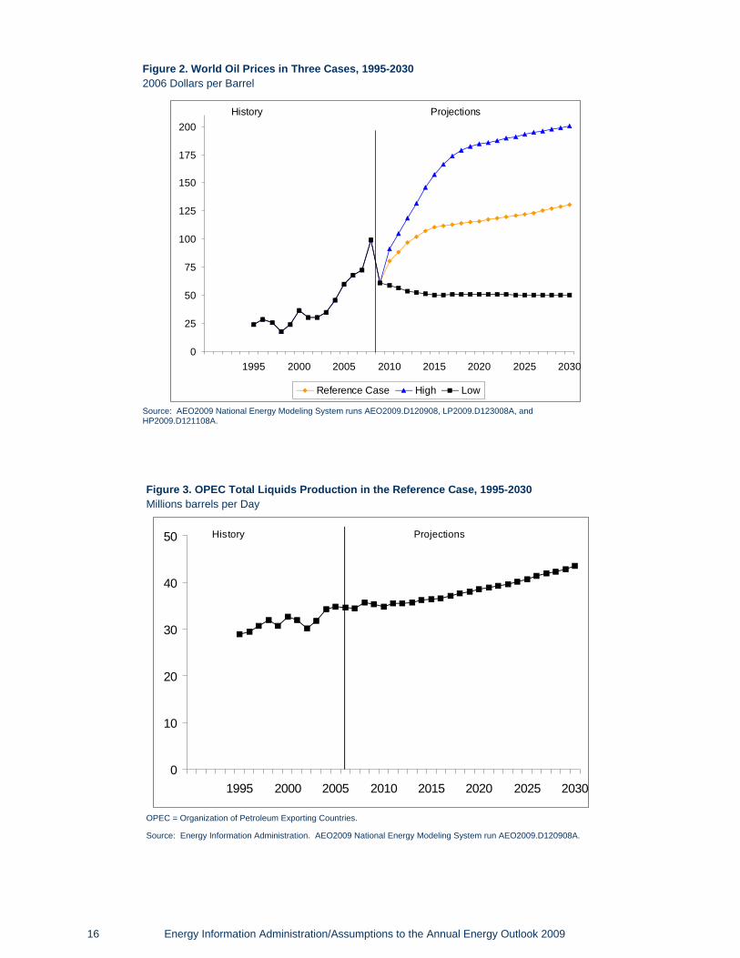
The world oil price is the annual average U.S. cost of imported low-sulfur light crude oil in PADD2. For the low,reference, and high oil price cases, prices reach $50, $130 and $200 per barrel in 2030, respectively, in 2007dollars. The reference case assumes that OPEC producers will continue to demonstrate a disciplined productionapproach. The low oil price case reflects a market where all oil production becomes more competitive andplentiful. The high oil price case could result from a more cohesive and market-assertive OPEC that reducesoverall production volumes. Thethree price scenarios are shown in Figure 2.
OPEC oil production is assumed to increase throughout the reference case projection, enabling theorganization to maintain an approximately constant market share over the projection period (Figure 3). OPECis assumed to be an important source of additional production because its member nations hold a major portionof the world’s total reserves—exceeding 927 billion barrels, about 70 percent of the world’s estimated total, atthe beginning of 2008.1
The reference case values for OPEC production are shown in Figure 3. Iraq oil production is assumed to notmaintain steady growth until after 2015. By 2030, Iraq is expected to increase production capacity to 4 millionbarrels per day with likely investment help from foreign sources. Non-OPEC liquids production is expected toincrease by just under one percent per year over the projection period, as advances in both exploration andextraction technologies result in an upward trend. The non-OPEC production path for the reference case isshown in Figure 4.
The non-U.S. oil production projections in the AEO2009 begin with country-level assumptions regarding oilresources. These resource estimates are taken in part from the USGS World Petroleum Assessment of2000 as well as from PennWell Publishing Company Oil and Gas Journal, summary of which is shown inTable 3.1.
The reference case growth rates for GDP for various regions in the world are shown in Table 3.2. Except for theUnited States, the GDP growth rate assumptions for non U.S. country/regions are taken from IEO2008.
Energy Information Administration/Assumptions to the Annual Energy Outlook 2009 15
Report #:DOE/EIA-0554(2009)Release date: March 2009Next release date: March 2010
16 Energy Information Administration/Assumptions to the Annual Energy Outlook 2009
0
25
50
75
100
125
150
175
200
1995 2000 2005 2010 2015 2020 2025 2030
Reference Case High Low
History Projections
Figure 2. World Oil Prices in Three Cases, 1995-2030
2006 Dollars per Barrel
Source: AEO2009 National Energy Modeling System runs AEO2009.D120908, LP2009.D123008A, andHP2009.D121108A.
0
10
20
30
40
50
1995 2000 2005 2010 2015 2020 2025 2030
History Projections
Figure 3. OPEC Total Liquids Production in the Reference Case, 1995-2030
Millions barrels per Day
OPEC = Organization of Petroleum Exporting Countries.
Source: Energy Information Administration. AEO2009 National Energy Modeling System run AEO2009.D120908A.

The values for growth in oil demand in the International Energy Module, which depend upon the oil pricelevels as well as GDP growth rates, are shown in Table 3.3 for the reference case by regions.
Energy Information Administration/Assumptions to the Annual Energy Outlook 2009 17
0
10
20
30
40
50
60
70
1995 2000 2005 2010 2015 2020 2025 2030
History Projections
Figure 4. Non-OPEC Total Liquids Production in the Reference Case, 1995-2030
Millions barrels per Day
OPEC = Organization of Petroleum Exporting Countries.
Source: Energy Information Administration. AEO2009 National Energy Modeling System run AEO2008.D120908A.

18 Energy Information Administration/Assumptions to the Annual Energy Outlook 2009
Region Proved Oil Reserves
Western Hemisphere 321.1
Western‘Europe 13.2
Asia-Pacific 34.3
Eastern Europe and F.S.U. 100
Middle East 748.3
Africa 114.8
Total World 1331.7
Total OPEC 927.5
Table 3.1. Worldwide Oil Reserves as of January 1, 2008(Billion Barrels)
Source: PennWell Corporation, Oil and Gas Journal, Vol 105. 48 (Dec 24, 2007).
Region Average Annual Percentage Change
OECD 2.3
OECD North America 2.6
OECD Europe 2.3
OECD Asia 1.8
Non-OECD 5.2
Non-OECD Europe and Eurasia 4.4
Non-OECD Asia 5.8
Middle East 4.0
Africa 4.5
Central and South America 3.9
Total World 4.0
Table 3.2. Average Annual Real Gross Domestic Product Rates, 2004-2030 (2000 Purchasing PowerParity Weights and Prices)
Source: For the U.S., Energy Informatin Administration, National Energy Modeling System run AEO2009.D120908A; for other countries, GlobalInsight, Inc., World Overview (Lexington, MA, January 2008)
Region Oil Demand Growth
OECD 0.02%
OECD North America 0.25%
OECD Europe 0.31%
OECD Asia -0.21%
Non-OECD 2.00%
Non-OECD Europe and Eurasia 1.07%
Non-OECD Asia 2.56%
Middle East 2.07%
Africa 1.38%
Central and South America 1.23%
Total World 0.94%
Table 3.3. Average Annual Growth Rates for Total Liquids Demand in the Reference Case, 2004-2030(Percent per Year)
Source: Energy Information Administration, AEO2008 National Energy Modeling System run: AEO2009.D120908A; and IEO2008 System for theAnalysis of Global Energy Markets (2008).

[1] PennWell Corporation, Oil and Gas Journal, Vol. 105.48 (December 24, 2007).
Energy Information Administration/Assumptions to the Annual Energy Outlook 2009 19
Notes and Sources


Residential Demand ModuleThe NEMS Residential Demand Module projects future residential sector energy requirements based onprojections of the number of households and the stock, efficiency, and intensity of use of energy-consumingequipment. The Residential Demand Module projections begin with a base year estimate of the housingstock, the types and numbers of energy-consuming appliances servicing the stock, and the “unit energyconsumption” by appliance (or UEC—in million Btu per household per year). The projection process addsnew housing units to the stock, determines the equipment installed in new units, retires existing housingunits, and retires and replaces appliances. The primary exogenous drivers for the module are housing startsby type (single-family, multifamily and mobile homes) and Census Division and prices for each energysource for each of the nine Census Divisions (see Figure 5). The Residential Demand Module also requiresprojections of available equipment and their installed costs over the projection horizon. Over time,
equipment efficiency tends to increase because of general technological advances and also because ofFederal and/or state efficiency standards. As energy prices and available equipment changes over theprojection horizon, the module includes projected changes to the type and efficiency of equipmentpurchased as well as projected changes in the usage intensity of the equipment stock.
The end-use services for which equipment stocks are modeled include space conditioning (heating andcooling), water heating, refrigeration, freezers, dishwashers, clothes washers, lighting, furnace fans, colortelevisions, personal computers, cooking, clothes drying, ceiling fans, coffee makers, spas, home securitysystems, microwave ovens, set-top boxes, home audio equipment, rechargeable electronics, andVCR/DVDs. In addition to the major equipment-driven end-uses, the average energy consumption perhousehold is projected for other electric and nonelectric appliances. The module’s output includes number
Energy Information Administration/Assumptions to the Annual Energy Outlook 2009 21
Pacific
East South Central
South Atlantic
MiddleAtlantic
NewEngland
WestSouth
Central
WestNorth
Central EastNorth
CentralMountain
AK
WAMT
WYID
NVUT
CO
AZNM
TX
OK
IA
KS MOIL
IN
KY
TN
MS AL
FL
GA
SC
NC
WV
PA NJ
MD
DE
NY
CT
VT ME
RIMA
NH
VA
WI
MI
OH
NE
SD
MNND
AR
LA
OR
CA
HI
Middle AtlanticNew England
East North CentralWest North Central
PacificWest South CentralEast South Central
South AtlanticMountain
2
4
3
1
Figure 5. United States Census Divisions
Source:Energy Information Administration,Office of Integrated Analysis and Forecasting.
Report #:DOE/EIA-0554(2009)Release date: March 2009Next release date: March 2010
of households, equipment stock, average equipment efficiencies, and energy consumed by service, fuel,and geographic location. The fuels represented are distillate fuel oil, liquefied petroleum gas, natural gas,kerosene, electricity, wood, geothermal, coal, and solar energy.
One of the implicit assumptions embodied in the Residential Demand Module is that, through 2030, there willbe no radical changes in technology or consumer behavior. No new regulations of efficiency beyond thosecurrently embodied in law or new government programs fostering efficiency improvements are assumed.Technologies which have not gained widespread acceptance today will generally not achieve significantpenetration by 2030. Currently available technologies will evolve in both efficiency and cost. In general, atthe same efficiency level, future technologies will be less expensive than those available today in real dollarterms. When choosing new or replacement technologies, consumers will behave similarly to the way theynow behave. The intensity of end-uses will change moderately in response to price changes. Electric enduses will continue to expand, but at a decreasing rate.1
Key Assumptions
Housing Stock Submodule
An important determinant of future energy consumption is the projected number of households. Base yearestimates for 2005 are derived from the Energy Information Administration’s (EIA) Residential EnergyConsumption Survey (RECS) (Table 4.1). The projection for occupied households is done separately foreach Census Division. It is based on the combination of the previous year’s surviving stock with projectedhousing starts provided by the NEMS Macroeconomic Activity Module. The housing stock submoduleassumes a constant survival rate (the percentage of households which are present in the current projectionyear, which were also present in the preceding year) for each type of housing unit; 99.6 percent forsingle-family units, 99.9 percent for multifamily units, and 97.6 percent for mobile home units. Projected fuelconsumption is dependent not only on the projected number of housing units, but also on the type andgeographic distribution of the houses. The intensity of space heating energy use varies greatly across thevarious climate zones in the United States. Also, fuel prevalence varies across the country—oil (distillate) ismore frequently used as a heating fuel in the New England and Middle Atlantic Census Divisions than in therest of the country, while natural gas dominates in the Midwest. An example of differences by housing type isthe more prevalent use of liquefied petroleum gas in mobile homes relative to other housing types.
Technology Choice Submodule
The key inputs for the Technology Choice Submodule are fuel prices by Census Division and characteristicsof available equipment (installed cost, maintenance cost, efficiency, and equipment life). Fuel prices aredetermined by an equilibrium process which considers energy supplies and demands and are passed to thissubmodule from the integrating module of NEMS. Energy price, combined with equipment UEC (which is afunction of efficiency), determines the operating costs of equipment. Equipment characteristics are
22 Energy Information Administration/Assumptions to the Annual Energy Outlook 2009
Census Division Single-family Units Multiple family Units Mobile Home Total Units
New England 3,392,944 1,899,981 173,072 5,465,996
Mid Atlantic 10,077,231 4,784,686 254,610 15,116,527
East North Central 14,091,216 3,233,929 424,271 17,749,416
West North Central 6,107,582 1,406,214 340,759 7,854,555
South Atlantic 14,823,560 4,910,592 1,962,563 21,696,715
East South Central 5,438,660 729,591 724,503 6,892,754
West South Central 8,892,255 2,120,675 1,109,901 12,122,831
Mountain 5,680,398 951,482 922,976 7,554,856
Pacific 11,150,078 4,456,348 1,030,541 16,636,967
United States 79,653,923 24,493,498 6,943,196 111,090,617
Table 4.1. 2005 Households
Source: U.S. Department of Energy, Energy Information Administration, 2005 Residential Energy Consumption Survey.

exogenous to the model and are modified to reflect both Federal standards and anticipated changes in themarket place. Table 4.2 lists capital cost and efficiency for selected residential appliances for the years 2007and 2020.
Table 4.3 provides the cost and performance parameters for representative distributed generationtechnologies. The AEO2009 model also incorporates endogenous “learning” for the residential distributedgeneration technologies, allowing for declining technology costs as shipments increase. For fuel cell andphotovoltaic systems, learning parameter assumptions for the AEO2009 reference case result in a 13percent reduction in capital costs each time the number of units shipped to the buildings sectors (residentialand commercial) doubles.
The Residential Demand Module projects equipment purchases based on a nested choice methodology.The first stage of the choice methodology determines the fuel and technology to be used, the second stagedetermines the efficiency of the selected equipment type. The equipment choices for cooling, water heating,and cooking are linked to the space heating choice for new construction. Technology and fuel choice forreplacement equipment uses a nested methodology similar to that for new construction, but includes (inaddition to the capital and installation costs of the equipment) explicit costs for technology switching (e.g.,costs for installing gas lines if switching from electricity or oil to gas, or costs for adding ductwork if switchingfrom electric resistance heat to central heating types). Also, for replacements, there is no linking of fuelchoice for water heating and cooking as is done for new construction. Technology switching uponreplacement is allowed for space heating, air conditioning, water heating, cooking and clothes drying.
Once the fuel and technology choice for a particular end use is determined, the second stage of the choicemethodology determines efficiency. In any given year, there are several available prototypes of varyingefficiency (minimum standard, medium low, medium high and highest efficiency). Efficiency choice is basedon a functional form and coefficients which give greater or lesser importance to the installed capital cost (firstcost) versus the operating cost. Generally, within a technology class, the higher the first cost, the lower theoperating cost. For new construction, efficiency choices are made based on the costs of both the heatingand cooling equipment and the building shell characteristics.
The parameters for the second stage efficiency choice are calibrated to the most recently available shipmentdata for the major residential appliances. Shipment efficiency data are obtained from industry associationswhich monitor shipments such as the Association of Home Appliance Manufacturers. Because of thiscalibration procedure, the model allows the relative importance of first cost versus operating cost to vary bygeneral technology and fuel type (e.g., natural gas furnace, electric heat pump, electric central airconditioner, etc.). Once the model is calibrated, it is possible to calculate (approximately) the apparent
Energy Information Administration/Assumptions to the Annual Energy Outlook 2009 23
Equipment TypeRelative
Performance1
2007Installed Cost
($2007)2 Efficiency3
2020Installed Cost
($2007)2 Efficiency3
Approximate Hurdle Rate
Electric Heat Pump MinimumBest
$3,800$6,700
13.017.0
$3,800$6,700
13.020.0
15%
Natural Gas Furnace MinimumBest
$1,900$3,050
0.800.96
$1,900$2,700
0.800.96
15%
Room Air Conditioner MinimumBest
$310$925
9.811.7
$310$875
9.812.0
140%
Central Air Conditioner MinimumBest
$3,000$5,700
13.021.0
$3,000$5,750
13.023.0
15%
Refrigerator (23.9 cubic ft in adjusted volume)
MinimumBest
$550$950
510417
$550$1000
510417
19%
Electric Water Heater MinimumBest
$400$1,400
0.902.4
$400$1,700
0.902.4
30%
Solar Water Heater N/A $3,500 2.0 $4,000 2.0 30%
Table 4.2. Installed Cost and Efficiency Ratings of Selected Equipment
1Minimum performance refers to the lowest efficiency equipment available. Best refers to the highest efficiency equipment available.2Installed costs are given in 2007 dollars in the original source document.3Efficiency measurements vary by equipment type. Electric heat pumps and central air conditioners are rated for cooling performance using theSeasonal Energy Efficiency Ratio (SEER); natural gas furnaces are based on Annual Fuel Utilization Efficiency; room air conditioners are based onEnergy Efficiency Ratio (EER); refrigerators are based on kilowatt-hours per year; and water heaters are based on Energy Factor (delivered Btudivided by input Btu).
Source: Navigant Consulting, EIA Technology Forecast Updates, Reference Number 20070831.1September 2007.

discount rates based on the relative weight given to the operating cost savings versus the weight given to thehigher cost of more efficient equipment. Hurdle rates in excess of 30 percent are common in the ResidentialDemand Module. The prevalence of such high apparent hurdle rates by consumers has led to the notion ofthe “efficiency gap” that is, there are many investments that could be made that provide rates of return inexcess of residential borrowing rates (15 to 20 percent for example). There are several studies whichdocument instances of apparent high discount rates.2 Once equipment efficiencies for a technology and fuelare determined, the installed efficiency for its entire stock is calculated.
Appliance Stock Submodule
The Appliance Stock Submodule is an accounting framework which tracks the quantity and averageefficiency of equipment by end use, technology, and fuel. It separately tracks equipment requirements fornew construction and existing housing units. For existing units, this module calculates equipment whichsurvives from previous years, allows certain end uses to further penetrate into the existing housing stock andcalculates the total number of units required for replacement and further penetration. Air conditioning andclothes drying are the two end uses not considered to be “fully penetrated.”
Once a piece of equipment enters into the stock, an accounting of its remaining life is begun. It is assumedthat all appliances survive a minimum number of years after installation. A fraction of appliances areremoved from the stock once they have survived for the minimum number of years. Between the minimumand maximum life expectancy, all appliances retire based on a linear decay function. For example, if anappliance has a minimum life of 5 years and a maximum life of 15 years, one tenth of the units (1 divided by15 minus 5) are retired in each of years 6 through 15. It is further assumed that, when a house is retired fromthe stock, all of the equipment contained in that house retires as well; i.e., there is no secondhand market forthis equipment. The assumptions concerning equipment lives are given in Table 4.4.
24 Energy Information Administration/Assumptions to the Annual Energy Outlook 2009
Technology Type Year of Introduction
AverageGenerating
Capacity (kW)
ElectricalEfficiency
CombinedEfficiency
(Elec. + Thermal)
Installed Capital
Cost ($2005 per
KW of Capacity)1
ServiceLife
Years
Solar Photovoltaic
2007 3.0 0.16 N/A $8,930 30
2010 3.5 0.18 N/A $8,467 30
2015 4.0 0.20 N/A $7,310 30
2020 5.0 0.22 N/A $6,154 30
2030 5.0 0.25 N/A $3,840 30
Fuel Cell 2007 10 0.308 0.697 $8,062 20
2010 10 0.320 0.699 $6,199 20
2015 10 0.335 0.705 $4,819 20
2020 10 0.350 0.712 $3,440 20
2030 10 0.360 0.723 $1,886 20
Table 4.3. Capital Cost and Performance Parameters of Selected Residential Distributed Generation Technologies
1Installed costs are given in 2005 dollars in the original source document.
Source: Solar Technology Specifications: Solar Energy Industries Association, Our Solar Power Future - The U.S. Photovoltaic Industry Roadmapthrough 2030 and Beyond (SEIA, September 2004). Fuel cells: Discovery Insights, LLC, "Installed Costs for Small CHP Systems - Estimates andProjections" (April 2005).

Fuel Consumption SubmoduleEnergy consumption is calculated by multiplying the vintage equipment stocks by their respective UECs.The UECs include adjustments for the average efficiency of the stock vintages, short term price elasticity ofdemand and “rebound” effects on usage (see discussion below), the size of new construction relative to theexisting stock, people per household and shell efficiency and weather effects (space heating and cooling).The various levels of aggregated consumption (consumption by fuel, by service, etc.) are derived from thesedetailed equipment-specific calculations.
Equipment Efficiency
The average energy consumption of a particular technology is initially based on estimates derived fromRECS 2005. Appliance efficiency is either derived from a long history of shipment data (e.g., the efficiency ofconventional air-source heat pumps) or assumed based on engineering information concerning typicalinstalled equipment (e.g., the efficiency of ground-source heat pumps). When the average efficiency iscomputed from shipment data, shipments going back as far as 20 to 30 years are combined withassumptions concerning equipment lifetimes. This allows for not only an average efficiency to becalculated, but also for equipment retirements to be vintaged—older equipment tends to be lower inefficiency and also tends to get retired before newer, more efficient equipment. Once equipment is retired,the Appliance Stock and Technology Choice Modules determine the efficiency of the replacementequipment. It is often the case that the retired equipment is replaced by substantially more efficientequipment.
As the stock efficiency changes over the simulation interval, energy consumption decreases in inverseproportion to efficiency. Also, as efficiency increases, the efficiency rebound effect (discussed below) willoffset some of the reductions in energy consumption by increased demand for the end-use service. Forexample, if the stock average for electric heat pumps is now 10 percent more efficient than in 2005, then allelse constant (weather, real energy prices, shell efficiency, etc.), energy consumption per heat pump wouldaverage about only 9 percent less.
Adjusting for the Size of Housing Units
Information derived from RECS 2005 indicates that new construction (post-1990) is on average roughly 26percent larger than the existing stock of housing. Estimates for the size of each new home built in theprojection period vary by type and region, and are determined by a log-trend projection based on historicaldata from the Bureau of the Census.3 For existing structures, it is assumed that about 1 percent ofhouseholds that existed in 2005 add about 600 square feet to the heated floor space in each year of theprojection period.4 The energy consumption for space heating, air conditioning, and lighting is assumed toincrease with the square footage of the structure. This results in an increase in the average size of thehousing stock from 1,632 to 1,934 square feet from 2005 through 2030.
Energy Information Administration/Assumptions to the Annual Energy Outlook 2009 25
Equipment Minimum Life Maximum Life
Heat Pumps 7 21
Central Forced-Air Furnaces 10 25
Hydronic Space Heaters 20 30
Room Air Conditioners 8 16
Central Air Conditioners 7 21
Gas Water Heaters 4 14
Electric Water Heaters 5 22
Cooking Stoves 16 21
Clothes Dryers 11 20
Refrigerators 7 26
Freezers 11 31
Table 4.4. Minimum and Maximum Life Expectancies of Equipment
Source: Lawrence Berkeley Laboratory, Baseline Data for the Residential Sector and Development of a Residential Forecasting Database, May1994, and analysis of RECS 2001 data.

Adjusting for Weather and Climate
Weather in any given year always includes short-term deviations from the expected longer-term average (orclimate). Recognition of the effect of weather on space heating and air conditioning is necessary to avoidinadvertently projecting abnormal weather conditions into the future. In the residential module, adjustmentsare made to space heating and air conditioning UECs by Census Division by their respective heating andcooling degree-days (HDD and CDD). A 10 percent increase in HDD would increase space heatingconsumption by 15 percent over what it would have otherwise been. Over the projection period, theresidential module uses a 10-year average for heating and cooling degree - days by Census Division,adjusted by projections in state population shifts.
Short-Term Price Effect and Efficiency Rebound
It is assumed that energy consumption for a given end-use service is affected by the marginal cost ofproviding that service. That is, all else equal, a change in the price of a fuel will have an opposite, but lessthan proportional, effect on fuel consumption. The current value for the short-term elasticity parameter is-0.15.5 This value implies that for a 1 percent increase in the price of a fuel, there will be a correspondingdecrease in energy consumption of -0.15 percent. Another way of affecting the marginal cost of providing aservice is through altered equipment efficiency. For example, a 10 percent increase in efficiency will reducethe cost of providing the end-use service by 10 percent. Based on the short-term efficiency reboundparameter, the demand for the service will rise by 1.5 percent (-10 percent multiplied by -0.15). Only spaceheating, cooling, and lighting are assumed to be affected by both elasticities and the efficiency reboundeffect.
Shell Efficiency
The shell integrity of the building envelope is an important determinant of the heating and cooling load foreach type of household. In the NEMS Residential Demand Module, the shell integrity is represented by anindex, which changes over time to reflect improvements in the building shell. The shell integrity index isdimensioned by vintage of house, type of house, fuel type, service (heating and cooling), and CensusDivision. The age, type, location, and type of heating fuel are important factors in determining the level ofshell integrity. Housing units that heat with electricity tend to have less air infiltration rates than homes thatuse other fuels. The age of homes are classified by new (post-2005) and existing. Existing homes arecharacterized by the RECS 2005 survey and are assigned a shell index value based on the mix of homesthat exist in the base year (2005). The improvement over time in the shell integrity of these homes is afunction of two factors—an assumed annual efficiency improvement and improvements made when real fuelprices increase (no price-related adjustment is made when fuel prices fall). For new construction, buildingshell efficiency is determined by the relative costs and energy bill savings for several levels of heating andcooling equipment, in conjunction with the building shell attributes. The packages represented in NEMSrange from homes that meet the International Energy Conservation Code (IECC)6 to homes that are builtwith the most efficient shell components. Shell efficiency in new homes would increase over time if energyprices rise, or the cost of more efficient equipment falls, all else equal.
Legislation and Regulations
Energy Improvement and Extension Act of 2008 (EIEA 2008)
EIEA 2008 extends and amends many of the tax credits that were made available to residential consumersin EPACT 2005. The tax credits for energy efficient equipment can now be claimed through 2016, while the$2000 cap for solar technologies has been removed. Additionally, the tax credit for ground-source(geothermal) heat pumps was increased to $2000. The production tax credits for dishwashers, clotheswashers, and refrigerators were extended by one to two years, depending on the efficiency level andproduct. See the EPACT 2005 section below for more details about product coverage.
Energy Independence and Security Act of 2007 (EISA 2007)
EISA 2007 contains several provisions that impact projections of residential energy use. Standards forgeneral service incandescent light bulbs are phased-in over 2012-2014, with a more restrictive standardspecified in 2020. It is estimated that these standards require 29 percent less watts per bulb in the first
26 Energy Information Administration/Assumptions to the Annual Energy Outlook 2009

phase-in, increasing to 67 percent in 2020. EISA also updates the dehumidifier standard specified inEPACT 2005, resulting in 7 percent increase in electricity savings, relative to the EPACT 2005 requirement.New efficiency standards for external power supplies are set for July 1, 2008, reducing electricity use in boththe active and no-load modes. Standards are also set for boilers (September 2012) and dishwashers(January 2010). Lastly, DOE is instructed to create standards for manufactured housing, requiringcompliance to the latest International Energy Conservation Code (IECC) by the end of 2011.
Energy Policy Act of 2005 (EPACT05)The passage of the EPACT05 in August 2005 provides additional minimum efficiency standards forresidential equipment and provides tax credits to producers and purchasers of energy efficient equipmentand builders of energy efficient homes. The standards contained in EPACT05 include: 190 watt maximumfor torchiere lamps in 2006; Dehumidifier standards for 2007 and 2012; and ceiling fan light kit standards in2007. Manufactured homes that are 30 percent better than the latest code, a $1000 tax credit can beclaimed in 2006 and 2007. Likewise, builders of homes that are 50 percent better than code can claim a$2000 credit over the same period. The builder tax credits and production tax credits are assumed to bepassed through to the consumer in the form of lower purchase cost. EPACT05 includes production taxcredits for energy efficient refrigerators, dishwashers, and clothes washers in 2006 and 2007, with dollaramounts varying by type of appliance and level of efficiency met, subject to annual caps. Consumers canclaim a 10 percent tax credit in 2006 and 2007 for several types of appliances specified by EPACT05,including: Energy efficient gas, propane, or oil furnaces or boilers, energy efficient central air conditioners,air and ground source heat pumps, hot water heaters, and windows. Lastly, consumers can claim a 30percent tax credit in 2006 and 2007 for purchases of solar PV, solar water heaters, and fuel cells, subject to acap.
National Appliance Energy Conservation Act of 1987The Technology Choice Submodule incorporates equipment standards established by the NationalAppliance Energy Conservation Act of 1987 (NAECA). Some of the NAECA standards implemented in themodule include: a Seasonal Energy Efficiency Rating (SEER) of 13.0 for central air conditioners and heatpumps; an Annual Fuel Utilization Efficiency (energy output over energy input) of 0.78 for oil and gasfurnaces; an Efficiency Factor of 0.90 for electric water heaters; and refrigerator standards that setconsumption limits to 510 kilowatt-hours per year in 2002.
Residential Alternative Cases
Technology CasesIn addition to the AEO2009 reference case, three side cases were developed to examine the effect ofequipment and building standards on residential energy use—a 2009 technology case, a best availabletechnology case, and a high technology case. These side cases were analyzed in stand-alone (notintegrated with the supply modules) NEMS runs and thus do not include supply-responses to the alteredresidential consumption patterns of the two cases. AEO2009 also analyzed integrated 2009 technology andhigh technology cases. The integrated 2009 technology case combines the 2009 technology cases of thefour end-use demand sectors, the electricity low fossil technology case, and the assumption of renewabletechnologies fixed at 2009 levels. The integrated high technology case uses the same approach, but for hightechnology.
The 2009 technology case assumes that all future equipment purchases are made based only on equipmentavailable in 2009. This case further assumes that existing building shell efficiencies will not improve beyond2009 levels.
The high technology case assumes earlier availability, lower costs, and/or higher efficiencies for moreadvanced equipment than the reference case. Equipment assumptions were developed by engineeringtechnology experts, considering the potential impact on technology given increased research anddevelopment into more advanced technologies.7 In the high technology case. All new construction isassumed to meet Energy Star specifications after 2016.
Energy Information Administration/Assumptions to the Annual Energy Outlook 2009 27

The best available technology case assumes that all equipment purchases from 2010 forward are based onthe highest available efficiency in the high technology case in a particular simulation year, disregarding theeconomic costs of such a case. This case is designed to show how much the choice of the highest-efficiencyequipment could affect energy consumption. In this case, all new construction is built to the most efficientspecifications after 2009.
28 Energy Information Administration/Assumptions to the Annual Energy Outlook 2009

[1] The Model Documentation Report contains additional details concerning model structure and operation.Refer to Energy Information Administration, Model Documentation Report: Residential Sector DemandModule of the National Energy Modeling System, DOE/EIA-M065(2008), (March 2009).
[2] Among the explanations often mentioned for observed high average implicit discount rates are: marketfailures, (i.e., cases where incentives are not properly aligned for markets to result in purchases based onenergy economics alone); unmeasured technology costs (i.e., extra costs of adoption which are not includedor difficult to measure like employee down-time); characteristics of efficient technologies viewed as lessdesirable than their less efficient alternatives (such as equipment noise levels or lighting qualitycharacteristics); and the risk inherent in making irreversible investment decisions. Examples of marketfailures/barriers include: decision makers having less than complete information, cases where energyequipment decisions are made by parties not responsible for energy bills (e.g., landlord/tenants,builders/home buyers), discount horizons which are truncated (which might be caused by mean occupancytimes that are less than the simple payback time and that could possibly be classified as an informationfailure), and lack of appropriate credit vehicles for making efficiency investments, to name a few. The use ofhigh implicit discount rates in NEMS merely recognizes that such rates are typically found to apply toenergy-efficiency investments.
[3] U.S. Bureau of Census, Series C25 Data from various years of publications.
[4] Sources: U.S. Bureau of Census, Annual Housing Survey 2001 and Professional Remodler, 2002 HomeRemodeling Study.
[5] See DAHL, CAROL, A Survey of Energy Demand Elasticities in Support of the Development of theNEMS, October 1993.
[6] The IECC established guidelines for builders to meet specific targets concerning energy efficiency withrespect to heating and cooling load.
[7] The high technology assumptions are based on Energy Information Administration, Technology ForecastUpdates-Residential and Commercial Building technologies-Advanced Adoption Case (NavigantConsulting, September 2007).
Energy Information Administration/Assumptions to the Annual Energy Outlook 2009 29
Notes and Sources


Commercial Demand ModuleThe NEMS Commercial Sector Demand Module generates projections of commercial sector energydemand through 2030. The definition of the commercial sector is consistent with EIA’s State Energy DataSystem (SEDS). That is, the commercial sector includes business establishments that are not engaged intransportation or in manufacturing or other types of industrial activity (e.g., agriculture, mining orconstruction). The bulk of commercial sector energy is consumed within buildings; however, street lights,pumps, bridges, and public services are also included if the establishment operating them is consideredcommercial. Since most of commercial energy consumption occurs in buildings, the commercial modulerelies on the data from the EIA Commercial Buildings Energy Consumption Survey (CBECS) forcharacterizing the commercial sector activity mix as well as the equipment stock and fuels consumed toprovide end use services.1
The commercial module projects consumption by fuel2 at the Census division level using prices from theNEMS energy supply modules, and macroeconomic variables from the NEMS Macroeconomic ActivityModule (MAM), as well as external data sources (technology characterizations, for example). Energydemands are projected for ten end-use services3 for eleven building categories4 in each of the nine Censusdivisions (see Figure 5). The model begins by developing projections of floorspace for the 99 buildingcategory and Census division combinations. Next, the ten end-use service demands required for theprojected floorspace are developed. The electricity generation and water and space heating supplied bydistributed generation and combined heat and power technologies are projected. Technologies are thenchosen to meet the projected service demands for the seven major end uses.5 Once technologies arechosen, the energy consumed by the equipment stock (both existing and purchased equipment) isdeveloped to meet the projected end-use service demands.6
Key Assumptions
The key assumptions made by the commercial module are presented in terms of the flow of the calculationsdescribed above. The sections below summarize the assumptions in each of the commercial modulesubmodules: floorspace, service demand, distributed generation, technology choice, and end-useconsumption. The submodules are executed sequentially in the order presented, and the outputs of eachsubmodule become the inputs to subsequently executed submodules. As a result, key projection drivers forthe floorspace submodule are also key drivers for the service demand submodule, and so on.
Floorspace SubmoduleFloorspace is projected by starting with the previous year's stock of floorspace and eliminating a portion torepresent the age-related removal of buildings. Total floorspace is the sum of the surviving floorspace plusnew additions to the stock derived from the MAM floorspace growth projection.7
Existing Floorspace and Attrition
Existing floorspace is based on the estimated floorspace reported in the 2003 Commercial Buildings EnergyConsumption Survey (Table 5.1). Over time, the 2003 stock is projected to decline as buildings are removedfrom service (floorspace attrition). Floorspace attrition is estimated by a logistic decay function, the shape ofwhich is dependent upon the values of two parameters: average building lifetime and gamma. The averagebuilding lifetime refers to the median expected lifetime of a particular building type. The gamma parametercorresponds to the rate at which buildings retire near their median expected lifetime. The current values forthe average building lifetime and gamma vary by building type as presented in Table 5.2.8
Energy Information Administration/Assumptions to the Annual Energy Outlook 2009 - 1/14/2009 DRAFT 31
Report #:DOE/EIA-0554(2009)Release date: March 2009Next release date: March 2010

New Construction Additions to Floorspace
The commercial module develops estimates of projected commercial floorspace additions by combining thesurviving floorspace estimates with the total floorspace projection from MAM. A total NEMS floorspaceprojection is calculated by applying the MAM assumed floorspace growth rate within each Census divisionand MAM building type to the corresponding NEMS Commercial Demand Module’s building types based onthe CBECS building type shares. The NEMS surviving floorspace from the previous year is then subtractedfrom the total NEMS floorspace projection for the current year to yield new floorspace additions.9
Service Demand Submodule
Once the building stock is projected, the Commercial Demand module develops a projection of demand forenergy-consuming services required for the projected floorspace. The module projects service demands forthe following explicit end-use services: space heating, space cooling, ventilation, water heating, lighting,cooking, refrigeration, personal computer office equipment, and other office equipment.10 The servicedemand intensity (SDI) is measured in thousand Btu of end-use service demand per square foot and differsacross service, Census division and building type. The SDIs are based on a hybrid engineering andstatistical approach of CBECS consumption data.11 Projected service demand is the product of square feetand SDI for all end uses across the eleven building categories with adjustments for changes in shellefficiency for space heating and cooling.
32 Energy Information Administration/Assumptions to the Annual Energy Outlook 2009 - 1/14/2009 DRAFT
Assem-bly
Educa-tion
FoodSales
FoodService
HealthCare Lodging Large
OfficeSmallOffice
Merc/Service
Ware-house Other Total
New England 431 299 75 45 48 374 282 320 819 411 351 3,452
Middle Atlantic 1,243 1,384 163 127 310 797 1,523 1,065 1,641 1,112 1,177 10,543
East North Central 1,355 1,990 218 248 316 549 1,297 1,129 2,148 2,023 1,152 12,424
West North Central 772 552 102 206 123 595 219 704 1,045 994 369 5,680
South Atlantic 1,161 2,445 223 433 469 939 1,173 1,065 3,391 1,836 865 13,999
East South Central 546 341 67 99 134 368 195 371 985 390 223 3,719
West South Central 965 1,198 197 232 235 387 916 501 2,076 1,740 575 9,022
Mountain 411 640 64 32 94 438 230 535 1,087 506 168 4,207
Pacific 809 1,027 146 232 176 649 1,028 915 2,051 1,066 515 8,613
United States 7,693 9,874 1,255 1,654 1,905 5,096 6,861 6,605 15,242 10,078 5,395 71,658
Table 5.1. 2003 Total Floorspace by Census Division and Principal Building Activity (Millions of Square Feet)
Note: Totals may not equal sum of components due to independent rounding.
Source: Energy Information Administration, 2003 Commercial Buildings Energy Consumption Survey Public Use Data
Assem-bly
Educa-tion
FoodSales
FoodService
HealthCare Lodging
LargeOffice
SmallOffice
Merc/Service
Ware-house Other
Median Expected Lifetime (years) 80 80 65 65 65 69 73 73 65 80 75
gamma 1.8 2.6 2.5 2.5 2.3 2.0 2.0 2.0 1.8 1.6 2.5
Table 5.2. Floorspace Attrition Parameters
Sources: Energy Information Administration, Commercial Buildings Energy Consumption Survey 1999, 1995, 1992, and 1989 Public Use Data, 1986Nonresidential Buildings Energy Consumption Survey, McGraw-Hill Construction Dodge Annual Starts - non residential building starts, and Journal ofBusiness and Economic Statistics, April 1986, Vol. 4, No. 2.

Shell Efficiency
The shell integrity of the building envelope is an important determinant of the heating and cooling loads foreach type of building. In the NEMS Commercial Demand Module, the shell efficiency is represented by anindex, which changes over time to reflect improvements in the building shell. This index is dimensioned bybuilding type and Census division and applies directly to heating. For cooling, the effects are computed fromthe index, but differ from heating effects, because of different marginal effects of shell integrity and becauseof internal building loads. In the AEO2009 reference case, shell improvements for new buildings are up to 60percent more efficient than the 2003 stock of similar buildings. Over the projection horizon, new buildingshells improve in efficiency by 7 percent relative to their efficiency in 2003. For existing buildings, efficiency isassumed to increase by 5 percent over the 2003 stock average. The shell efficiency index affects the spaceheating and cooling service demand intensities causing changes in fuel consumed for these services as theshell integrity improves.
Distributed Generation and Combined Heat and PowerProgram driven installations of solar photovoltaic systems are based on information from DOE’sPhotovoltaic and Million Solar Roofs programs as well as DOE and industry news releases, State-levelprogram information and the National Renewable Energy Laboratory’s Renewable Electric Plant InformationSystem. Historical data from Form EIA-860, Annual Electric Generator Report, are used to derive electricitygeneration for 2004 through 2007 by Census division, building type and fuel. A projection of distributedgeneration and combined heat and power (CHP) of electricity is developed based on the economic returnsprojected for distributed generation and CHP technologies. The model uses a detailed cash-flow approachto estimate the internal rate of return for an investment. Penetration assumptions for distributed generationand CHP technologies are a function of the estimated internal rate of return relative to purchased electricity.Table 5.3 provides the cost and performance parameters for representative distributed generation and CHPtechnologies.
The model also incorporates endogenous “learning” for new distributed generation and CHP technologies,allowing for declining technology costs as shipments increase. For fuel cell and photovoltaic systems,parameter assumptions for the AEO2009 reference case result in a 13 percent reduction in capital costseach time the number of units shipped to the buildings sectors (residential and commercial) doubles.Doubling the number of microturbines shipped results in a 10 percent reduction in capital costs and doublingthe number of distributed wind systems shipped results in a 3 percent reduction.
Technology Choice SubmoduleThe technology choice submodule develops projections of the results of the capital purchase decisions forequipment fueled by the three major fuels (electricity, natural gas, and distillate fuel). Capital purchasedecisions are driven by assumptions concerning behavioral rule proportions and time preferences,described below, as well as projected fuel prices, average utilization of equipment (the capacity factors),relative technology capital costs, and operating and maintenance (O&M) costs.
Decision Types
In each projection year, equipment is potentially purchased for three “decision types”. Equipment must bepurchased for newly added floorspace and to replace the portion of equipment in existing floorspace that isprojected to wear out.12 Equipment is also potentially purchased for retrofitting equipment that has becomeeconomically obsolete. The purchase of retrofit equipment occurs only if the annual operating costs of acurrent technology exceed the annualized capital and operating costs of a technology available as a retrofitcandidate.
Behavioral Rules
The commercial module allows the use of three alternate assumptions about equipment choice behavior.These assumptions constrain the equipment selections to three choice sets, which are progressively morerestrictive. The choice sets vary by decision type and building type:
Energy Information Administration/Assumptions to the Annual Energy Outlook 2009 33

• Unrestricted Choice Behavior - This rule assumes that commercial consumers consider all types ofequipment that meet a given service, across all fuels, when faced with a capital purchase decision.
• Same Fuel Behavior - This rule restricts the capital purchase decision to the set of technologies thatconsume the same fuel that currently meets the decision maker’s service demand.
34 Energy Information Administration/Assumptions to the Annual Energy Outlook 2009 - 1/14/2009 DRAFT
Technology Type Year
AverageGeneratingCapacity(kW)
ElectricalEfficiency
CombinedEfficiency(Elec.+Thermal)
Installed CapitalCost ($2005 per kW of Capacity)*
Service Life (Years)
Solar Photovoltaic 20062010
3032
0.160.18
N/AN/A
$6,385$5,962
3030
201520202025
354040
0.200.220.22
N/AN/AN/A
$4,428$3,830$3,802
303030
2030 45 0.25 N/A $3,200 30
Fuel Cell 2006 200 0.38 0.70 $6,898 202010 200 0.44 0.66 $6,219 202015202020252030
200200200200
0.450.470.480.49
0.670.690.700.72
$5,203$4,187$3,647$3,108
20202020
Natural Gas Engine 200620102015202020252030
300300300300300300
0.310.320.320.320.330.33
0.770.780.780.780.790.79
$2,081$1,878$1,714$1,551$1,343$1,134
202020202020
Oil-Fired Engine 200620102015202020252030
300300300300300300
0.340.340.350.350.360.36
0.730.740.740.740.780.82
$2,514$2,268$2.071$1,873$1,622$1,370
202020202020
Natural Gas Turbine 200620102015202020252030
100010001000100010001000
0.220.230.240.240.250.26
0.680.680.680.690.690.70
$1,955$1,775$1,684$1,593$1,511$1,429
202020202020
Natural Gas Micro Turbine
200620102015202020252030
250250250250250250
0.290.290.310.330.340.36
0.590.600.600.610.620.63
$2,751$2,328$1,981$1,634$1,343$1,052
202020202020
Wind200620102015202020252030
303235404050
0.130.130.130.130.130.13
N/AN/AN/AN/AN/AN/A
$3,959$3,736$3,691$3,510$3,338$3,174
303030303030
Table 5.3. Capital Cost and Performance Parameters of Selected Commercial Distributed Generation Technologies
*Installed costs are given in 2005 dollars in the original source document. Costs for solar photovoltaic, fuel cell, microturbine, and wind technologiesinclude learning effects.
Sources: Energy Information Administration, Commercial and Industrial CHP Technology Cost and Performance Data Analysis for EIA's NEMS,Decision Analysis Corporation and Discovery Insights LLC., February 2006, National Renewable Energy Laboratory, Gas-Fired Distributed EnergyResource Technology Characterizations: Reference Number NREL/TP-620-34783, November 2003, Discovery Insights, LLC, "Installed Costs forSmall CHP Systems - Estimates and Projections" (April 2005) California Solar Initiative program data, and Solar Energy Industries Association, OurSolar Power Future - The U.S. Photovoltaic Industry Roadmap through 2030 and Beyond, (SEIA, September 2004).

• Same Technology Behavior - Under this rule, commercial consumers consider only the availablemodels of the same technology and fuel that currently meet service demand, when facing a capitalstock decision.
Under any of the above three behavior rules, equipment that meets the service at the lowest annualizedlifecycle cost is chosen. Table 5.5 illustrates the proportions of floorspace subject to the different behaviorrules for space heating technology choices in large office buildings.
Time Preferences
Commercial building owners' time preferences regarding current versus future expenditures are assumed tobe distributed among seven alternate time preference premiums (Table 5.6). Adding the risk-adjusted timepreference premiums to the 10-year Treasury Bill rate from MAM results in implicit discount rates, alsoknown as hurdle rates, applicable to the assumed proportions of commercial floorspace. The effect of theuse of this distribution of discount rates is to prevent a single technology from dominating purchasedecisions in the lifecycle cost comparisons. The distribution used for AEO2009 assigns some floorspace avery high discount or hurdle rate to simulate floorspace which will never retrofit existing equipment and whichwill only purchase equipment with the lowest capital cost. Discount rates for the remaining six segments ofthe distribution get progressively lower, simulating increased sensitivity to the fuel costs of the equipmentthat is purchased. The proportion of floorspace assumed for the 0.0 time preference premium represents anestimate of the Federally owned commercial floorspace that is subject to purchase decisions in a given year.The Federal sector is expected to purchase energy-efficient equipment to meet the Federal buildingsperformance standards of the Energy Policy Act of 2005 and the Energy Independence and Security Act of2007 whenever cost effective. For Federal purchase decisions relating to energy conservation, costeffectiveness is determined using a discount rate based on long-term Treasury bond rates, approximated inthe commercial module by the 10-year Treasury Bill rate. For lighting, the proportion of floorspace assumedfor the 0.0 time preference premium is increased to include all Federal floorspace starting in 2009 torepresent the EISA 2007 provision that all Federal buildings be equipped with energy efficient lightingfixtures and bulbs to the maximum extent feasible, including when replacing bulbs in existing fixtures.
Energy Information Administration/Assumptions to the Annual Energy Outlook 2009 - 1/14/2009 DRAFT 35
Proportion of Floorspace-AllProportion of Floorspace-Lighting
(2009 and later) Time Preference PremiumServices (Except Lighting 2009
and later)27.0 27.0 1000.0
25.4 25.4 152.9
20.4 20.4 55.4
16.2 16.2 30.9
10.0 7.9 19.9
0.8 0.6 13.6
0.2 2.5 0.0
100.0 100.0 --
Table 5.6. Assumed Distribution of Risk-adjusted Time Preference Premiums(Percent)
Source: Energy Information Administration, Model Documentation Report: Commercial Sector Demand Module of the National Energy ModelingSystem, DOE/EIA-M066(2009) (March 2009).
Unrestricted Same Fuel Same Technology Total
New Equipment Decision 21 30 49 100
Replacement Decision 7 31 62 100
Retrofit Decision 1 4 95 100
Table 5.5. Assumed Behavior Rules for Choosing Space Heating Equipment in Large Office Buildings(Percent)
Source: Energy Information Administration, Model Documentation Report: Commercial Sector Demand Module of the National Energy ModelingSystem, DOE/EIA-M066(2009) (March 2009).

The distribution of hurdle rates used in the commercial module is also affected by changes in fuel prices. If afuel’s price rises relative to its price in the base year (2003), the nonfinancial portion of each hurdle rate in thedistribution decreases to reflect an increase in the relative importance of fuel costs, expected in anenvironment of rising prices. Parameter assumptions for AEO2009 result in a 30 percent reduction in thenonfinancial portion of a hurdle rate if the fuel price doubles. If the risk-adjusted time preference premiuminput by the model user results in a hurdle rate below the assumed financial discount rate for the commercialsector, 15 percent, with base year fuel prices (such as the rate given in Table 5.6 for the Federal sector), noresponse to increasing fuel prices is assumed.
Technology Characterization Database
The technology characterization database organizes all relevant technology data by end use, fuel, andCensus division. Equipment is identified in the database by a technology index as well as a vintage index,the index of the fuel it consumes, the index of the service it provides, its initial market share, the Censusdivision index for which the entry under consideration applies, its efficiency (or coefficient of performance orefficacy in the case of lighting equipment), installed capital cost per unit of service demand satisfied,operating and maintenance cost per unit of service demand satisfied, average service life, year of initialavailability, and last year available for purchase. Equipment may only be selected to satisfy service demandif the year in which the decision is made falls within the window of availability. Equipment acquired prior tothe lapse of its availability continues to be treated as part of the existing stock and is subject to replacementor retrofitting. This flexibility in limiting equipment availability allows the direct modeling of equipmentefficiency standards. Table 5.7 provides a sample of the technology data for space heating in the NewEngland Census division.
An option to allow endogenous price-induced technological change has been included in the determinationof equipment costs and availability for the menu of equipment. This concept allows future technologiesfaster diffusion into the market place if fuel prices increase markedly for a sustained period of time. Theoption was not exercised for the AEO2009 model runs.
End-Use Consumption Submodule
The end-use consumption submodule calculates the consumption of each of the three major fuels for the tenend-use services plus fuel consumption for combined heat and power and district services. For the tenend-use services, energy consumption is calculated as the end-use service demand met by a particular typeof equipment divided by its efficiency and summed over all existing equipment types. This calculationincludes dimensions for Census division, building type, and fuel. Consumption of the five minor fuels isprojected based on historical trends.
Equipment Efficiency
The average energy consumption of a particular appliance is based initially on estimates derived from the2003 CBECS. As the stock efficiency changes over the model simulation, energy consumption decreasesnearly, but not quite proportionally to the efficiency increase. The difference is due to the calculation ofefficiency using the harmonic average and also the efficiency rebound effect discussed below. For example,if on average, electric heat pumps are now 10 percent more efficient than in 2003, then all else constant(weather, real energy prices, shell efficiency, etc.), energy consumption per heat pump would now averageabout 9 percent less. The Service Demand and Technology Choice Submodules together determine theaverage efficiency of the stocks used in adjusting the initial average energy consumption.
Adjusting for Weather and Climate
Weather in any given year always includes short-term deviations from the expected longer-term average (orclimate). Recognition of the effect of weather on space heating and air conditioning is necessary to avoidprojecting abnormal weather conditions into the future. In the commercial module, proportionateadjustments are made to space heating and air conditioning demand by Census division. Theseadjustments are based on National Oceanic and Atmospheric Administration (NOAA) data for HeatingDegree Days (HDD) and Cooling Degree Days (CDD). A 10 percent increase in HDD would increase spaceheating consumption by 10 percent over what it would have been otherwise. The commercial module uses a10-year average for HDD and CDD by Census division, adjusted over the projection period by projections forstate population shifts.
36 Energy Information Administration/Assumptions to the Annual Energy Outlook 2009
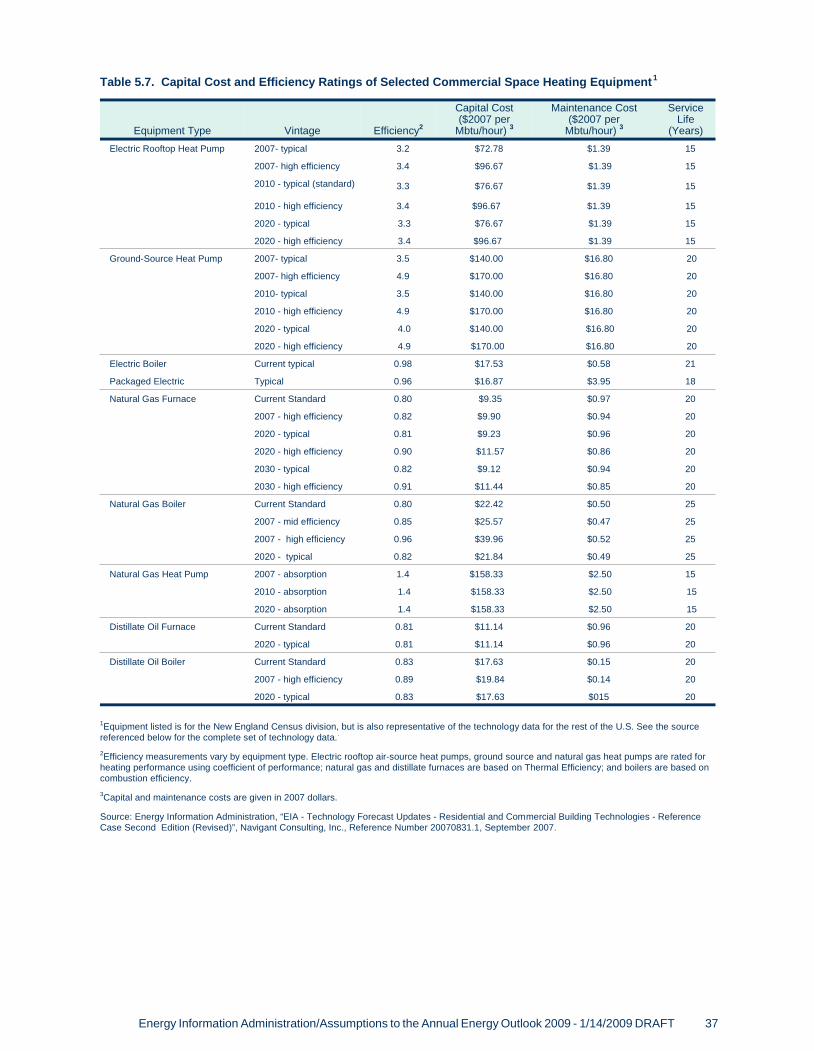
Energy Information Administration/Assumptions to the Annual Energy Outlook 2009 - 1/14/2009 DRAFT 37
Equipment Type Vintage Efficiency2
Capital Cost($2007 per
Mbtu/hour) 3
Maintenance Cost($2007 per
Mbtu/hour) 3
ServiceLife
(Years)Electric Rooftop Heat Pump 2007- typical 3.2 $72.78 $1.39 15
2007- high efficiency 3.4 $96.67 $1.39 15
2010 - typical (standard) 3.3 $76.67 $1.39 15
2010 - high efficiency 3.4 $96.67 $1.39 15
2020 - typical 3.3 $76.67 $1.39 15
2020 - high efficiency 3.4 $96.67 $1.39 15
Ground-Source Heat Pump 2007- typical 3.5 $140.00 $16.80 20
2007- high efficiency 4.9 $170.00 $16.80 20
2010- typical 3.5 $140.00 $16.80 20
2010 - high efficiency 4.9 $170.00 $16.80 20
2020 - typical 4.0 $140.00 $16.80 20
2020 - high efficiency 4.9 $170.00 $16.80 20
Electric Boiler Current typical 0.98 $17.53 $0.58 21
Packaged Electric Typical 0.96 $16.87 $3.95 18
Natural Gas Furnace Current Standard 0.80 $9.35 $0.97 20
2007 - high efficiency 0.82 $9.90 $0.94 20
2020 - typical 0.81 $9.23 $0.96 20
2020 - high efficiency 0.90 $11.57 $0.86 20
2030 - typical 0.82 $9.12 $0.94 20
2030 - high efficiency 0.91 $11.44 $0.85 20
Natural Gas Boiler Current Standard 0.80 $22.42 $0.50 25
2007 - mid efficiency 0.85 $25.57 $0.47 25
2007 - high efficiency 0.96 $39.96 $0.52 25
2020 - typical 0.82 $21.84 $0.49 25
Natural Gas Heat Pump 2007 - absorption 1.4 $158.33 $2.50 15
2010 - absorption 1.4 $158.33 $2.50 15
2020 - absorption 1.4 $158.33 $2.50 15
Distillate Oil Furnace Current Standard 0.81 $11.14 $0.96 20
2020 - typical 0.81 $11.14 $0.96 20
Distillate Oil Boiler Current Standard 0.83 $17.63 $0.15 20
2007 - high efficiency 0.89 $19.84 $0.14 20
2020 - typical 0.83 $17.63 $015 20
Table 5.7. Capital Cost and Efficiency Ratings of Selected Commercial Space Heating Equipment1
1Equipment listed is for the New England Census division, but is also representative of the technology data for the rest of the U.S. See the sourcereferenced below for the complete set of technology data..
2Efficiency measurements vary by equipment type. Electric rooftop air-source heat pumps, ground source and natural gas heat pumps are rated forheating performance using coefficient of performance; natural gas and distillate furnaces are based on Thermal Efficiency; and boilers are based oncombustion efficiency.3Capital and maintenance costs are given in 2007 dollars.
Source: Energy Information Administration, “EIA - Technology Forecast Updates - Residential and Commercial Building Technologies - ReferenceCase Second Edition (Revised)”, Navigant Consulting, Inc., Reference Number 20070831.1, September 2007.

Short-Term Price Effect and Efficiency Rebound
It is assumed that energy consumption for a given end-use service is affected by the marginal cost ofproviding that service. That is, all else equal, a change in the price of a fuel will have an inverse, but less thanproportional, effect on fuel consumption. The current value for the short-term price elasticity parameter is-0.25 for all major end uses except refrigeration. A value of -0.1 is currently used for commercialrefrigeration. A value of -0.05 is currently used for PC and non-PC office equipment and other minor uses ofelectricity. For example, for lighting this value implies that for a 1 percent increase in the price of a fuel, therewill be a corresponding decrease in energy consumption of 0.25 percent. Another way of affecting themarginal cost of providing a service is through equipment efficiency. As equipment efficiency changes overtime, so will the marginal cost of providing the end-use service. For example, a 10 percent increase inefficiency will reduce the cost of providing the service by 10 percent. The short-term elasticity parameter forefficiency rebound effects is -0.15 for affected end uses; therefore, the demand for the service will rise by 1.5percent (-10 percent x -0.15). Currently, all services are affected by the short-term price effect and servicesaffected by efficiency rebound are space heating and cooling, water heating, ventilation and lighting.
Legislation and Regulations
Energy Improvement and Extension Act of 2008 (EIEA08)
The EIEA08 legislation passed in October 2008 extends the Business Investment Tax Credit provisions ofthe Energy Policy Act of 2005 and expands the credit to include additional technologies. The BusinessInvestment Tax Credits of 30 percent for solar energy systems and fuel cells and 10 percent formicroturbines are extended through 2016. The cap on the fuel cell credit has been increased from $500 to$1,500 per half kilowatt of capacity. The EIEA08 provisions expand the Investment Tax Credit to include a10-percent credit for CHP systems and ground-source heat pumps and a 30-percent credit for wind turbineswith the wind credit capped at $4,000. The expanded credits are available for systems installed through2016. These credits are directly incorporated into the cash-flow approach for distributed generationsystems, including CHP, and factored into the installed capital cost assumptions for solar hot water heatersand ground-source heat pumps.
Energy Independence and Security Act of 2007 (EISA07)
The EISA07 legislation passed in December 2007 provides standards for the following explicitly modeledcommercial equipment. The EISA07 requires specific energy efficiency measures in commercial walk-incoolers and walk-in freezers effective January 1, 2009. Incandescent and halogen lamps must meetstandards for maximum allowable wattage based on lumen output starting in 2012 and metal halide lampfixtures using lamps between 150 and 500 watts are required to have a minimum ballast efficiency rangingfrom 88 to 94 percent, depending on ballast type, effective January 1, 2009.
The EISA07 requirement for Federal buildings to use energy efficient lighting fixtures and bulbs to themaximum extent possible is represented by adjusting the proportion of the commercial sector assumed touse the 10-year Treasury Bill rate as an implicit discount or hurdle rate for lighting.
Energy Policy Act of 2005 (EPACT05)
The passage of the EPACT05 in August 2005 provides additional minimum efficiency standards forcommercial equipment. Some of the standards for explicitly modeled equipment, effective January 1, 2010,include: an Energy Efficiency Rating (EER) ranging from 10.8 to 11.2 for small package air conditioning andheating equipment; daily electricity consumption limits by volume for commercial refrigerators, freezers, andrefrigerator-freezers; and electricity consumption limits per 100 pounds of ice produced based on equipmenttype and capacity for automatic ice makers. The EPACT05 adds standards for medium base compactfluorescent lamps effective January 1, 2006, for ballasts for Energy Saver fluorescent lamps effective in2009 and 2010, and bans the manufacture or import of mercury vapor lamp ballasts effective January 1,2008.
Several efficiency standards in the EPACT05 pertain to equipment not explicitly represented in the NEMSCommercial Demand Module. For low voltage dry-type transformers, effects of the standard are included inestimating the share of projected miscellaneous electricity use attributable to transformer losses. For
38 Energy Information Administration/Assumptions to the Annual Energy Outlook 2009 - 1/14/2009 DRAFT

illuminated exit signs, traffic signals, and commercial prerinse spray valves, assumed energy reductions arecalculated based on per-unit savings relative to a baseline unit and the estimated share of installed units andsales that already meet the standard. Total projected reductions are phased in over time to account for stockturnover. Under the EPACT05 standards, illuminated exit signs and traffic signal modules must meetENERGY STAR program requirements as of January 1, 2006. The requirements limit input power demandto 5 watts or less per face for exit signs. Nominal wattages for traffic signal modules are limited to 8 to 15watts, based on module type. Effective January 1, 2007, low voltage dry-type distribution transformers arerequired to meet the National Electrical Manufacturers Association Class I Efficiency Levels with minimumefficiency levels ranging from 97 percent to 98.9 percent based on output. Commercial prerinse sprayvalves13 must have a maximum flow rate of 1.6 gallons per minute, effective January 1, 2006 with energyreductions attributed to hot water use.
The EPACT05 expands the Business Investment Tax Credit to 30 percent for solar property installed in 2006and 2007. Business Investment Tax Credits of 30 percent for fuel cells and 10 percent for microturbinepower plants are also available for property installed in 2006 and 2007. The EPACT05 tax credit provisionswere extended in December 2006 to cover equipment installed in 2008. These credits are directlyincorporated into the cash-flow approach for distributed generation systems and factored into the installedcapital cost assumptions for solar hot water heaters.
Energy Policy Act of 1992 (EPACT92)
A key assumption incorporated in the technology selection process is that the equipment efficiencystandards described in the EPACT92 constrain minimum equipment efficiencies. The effects of standardsare modeled by modifying the technology database to eliminate equipment that no longer meets minimumefficiency requirements. For standards effective January 1, 1994, affected equipment includes electric heatpumps—minimum heating system performance factor of 6.8, gas and oil-fired boilers—minimumcombustion efficiency of 0.8 and 0.83, respectively, gas and oil-fired furnaces—minimum thermal efficiencyof 0.8 and 0.81, respectively, fluorescent lighting—minimum efficacy of 75 lumens per watt, incandescentlighting—minimum efficacy of 16.9 lumens per watt, air-cooled air conditioners—minimum energy efficiencyratio of 8.9, electric water heaters—minimum energy factor of 0.85, and gas and oil water heaters—minimumthermal efficiency of 0.78. Updated standards are effective October 29, 2003 for gas waterheaters—minimum thermal efficiency of 0.8. An additional standard affecting fluorescent lamp ballasts iseffective April 1, 2005. The standard mandates electronic ballasts with a minimum ballast efficacy factor of1.17 for 4-foot, 2-lamp ballasts and 0.63 for 8-foot, 2-lamp ballasts.
The 10 percent Business Investment Tax Credit for solar energy property included in EPACT92 is directlyincorporated into the cash-flow approach for projecting distributed generation by commercial photovoltaicsystems. For solar hot water heaters, the tax credit is factored into the installed capital cost assumptionsused in the technology choice submodule.
Energy Efficiency Programs
Several energy efficiency programs affect the commercial sector. These programs are designed to stimulateinvestment in more efficient building shells and equipment for heating, cooling, lighting, and other end uses.The commercial module includes several features that allow projected efficiency to increase in response tovoluntary programs (e.g., the distribution of risk-adjusted time preference premiums and shell efficiencyparameters). Retrofits of equipment for space heating, air conditioning and lighting are incorporated in thedistribution of premiums given in Table 14. Also the shell efficiency of new and existing buildings is assumedto increase from 2003 through 2030. Shells for new buildings increase in efficiency by 7 percent over thisperiod, while shells for existing buildings increase in efficiency by 5 percent.
Energy Information Administration/Assumptions to the Annual Energy Outlook 2009 39

Commercial Alternative Cases
Technology Cases
In addition to the AEO2009 reference case, three side cases were developed to examine the effect ofequipment and building standards on commercial energy use—a 2009 technology case, a high technologycase, and a best available technology case. These side cases were analyzed in stand-alone (not integratedwith the NEMS demand and supply modules) buildings (residential and commercial) modules runs and thusdo not include supply-responses to the altered commercial consumption patterns of the three cases.AEO2009 also analyzed an integrated high technology case, which combines the high technology cases ofthe four end-use demand sectors, the electricity high fossil technology case, the low nuclear cost case, andthe low renewable cost case, and an integrated 2009 technology case, which combines the 2009 technologycases of the end-use demand sectors, the electricity low fossil technology case, and the high renewable costcase.
The 2009 technology case assumes that all future equipment purchases are made based only on equipmentavailable in 2009. This case assumes building shell efficiency to be fixed at 2009 levels. In the referencecase, existing building shells are allowed to increase in efficiency by 5 percent over 2003 levels, and newbuilding shells improve by 7 percent by 2030 relative to new buildings in 2003.
The high technology case assumes earlier availability, lower costs, and/or higher efficiencies for moreadvanced equipment than the reference case. Equipment assumptions were developed by engineeringtechnology experts, considering the potential impact on technology given increased research anddevelopment into more advanced technologies. In the high technology case, building shell efficiencies areassumed to improve 25 percent more than in the reference case after 2009. Existing building shells,therefore, increase by 6.25 percent relative to 2003 levels and new building shells by 8.75 percent relative totheir efficiency in 2003 by 2030.
The best available technology case assumes that all equipment purchases after 2009 are based on thehighest available efficiency in the high technology case in a particular simulation year, disregarding theeconomic costs of such a case. It is designed to show how much the choice of the highest-efficiencyequipment could affect energy consumption. Shell efficiencies in this case are assumed to improve 50percent more than in the reference case after 2009, i.e., existing shells increase by 7.5 percent relative to2003 levels and new building shells by 10.5 percent relative to their efficiency in 2003 by 2030.
Fuel shares, where appropriate for a given end use, are allowed to change in the technology cases as theavailable technologies from each technology type compete to serve certain segments of the commercialfloorspace market. For example, in the best available technology case, the most efficient gas furnacetechnology competes with the most efficient electric heat pump technology. This contrasts with thereference case, in which, a greater number of technologies for each fuel with varying efficiencies allcompete to serve the heating end use. In general, the fuel choice will be affected as the available choicesare constrained or expanded, and will thus differ across the cases.
Two sensitivities that focus on electricity generation incorporate alternative assumptions for non-hydrorenewable energy technologies in the power sector, the industrial sector, and the buildings sectors, includingresidential and commercial photovoltaic and wind systems. In each of these cases, assumptions regardingnon-renewable technologies are not changed from the reference case.
The high renewable cost case assumes that the cost and performance characteristics for residential andcommercial photovoltaic and wind systems remain fixed at 2009 levels through the projection horizon.
The low renewable cost case assumes that costs for residential and commercial photovoltaic and windsystems are 25 percent lower than reference case cost estimates by 2030.
40 Energy Information Administration/Assumptions to the Annual Energy Outlook 2009 - 1/14/2009 DRAFT

[1] Energy Information Administration, 2003 Commercial Buildings Energy Consumption Survey (CBECS)Public Use Files, web site www.eia.doe.gov/emeu/cbecs/cbecs2003/public_use_2003/cbecs_pubdata2003. html.
[2] The fuels accounted for by the commercial module are electricity, natural gas, distillate fuel oil, residualfuel oil, liquefied petroleum gas (LPG), coal, motor gasoline, and kerosene. Current commercial use ofbiomass (wood, Municipal solid waste) is also included. In addition to these fuels the use of solar energy isprojected based on an exogenous estimate of projected solar photovoltaic system installations under theMillion Solar Roofs program, State and local incentive programs, and the potential endogenous penetrationof solar photovoltaic systems and solar thermal water heaters. The use of wind energy is projected based onan estimate of existing distributed wind turbines and the potential endogenous penetration of wind turbinesin the commercial sectors.
[3] The end-use services in the commercial module are heating, cooling, water heating, ventilation, cooking,lighting, refrigeration, PC and non-PC office equipment and a category denoted other to account for all otherminor end uses.
[4] The 11 building categories are assembly, education, food sales, food services, health care, lodging,large offices, small offices, mercantile/services, warehouse and other.
[5] Minor end uses are modeled based on penetration rates and efficiency trends.
[6] The detailed documentation of the commercial module contains additional details concerning modelstructure and operation. Refer to Energy Information Administration, Model Documentation Report:Commercial Sector Demand Module of the National Energy Modeling System, DOE/EIA M066(2008), (June2008).
[7] The commercial floorspace equations of the Macroeconomic Activity Model are estimated using theMcGraw-Hill Construction Research & Analytics database of historical floorspace estimates. TheMcGraw-Hill Construction estimate for commercial floorspace in the U.S. is approximately 16 percent lowerthan the estimate obtained from the CBECS used for the Commercial module. See F.W. Dodge, BuildingStock Database Methodology and 1991 Results, Construction Statistics and Forecasts, F.W. Dodge,McGraw-Hill.
[8] The commercial module performs attrition for 9 vintages of floorspace developed using stock estimatesfrom the previous 5 CBECS and historical floorspace additions data from McGraw-Hill Construction data.
[9] In the event that the computation of additions produce a negative value for a specific building type, it isassumed to be zero.
[10] “Other office equipment” includes copiers, fax machines, typewriters, cash registers, server computers,and other miscellaneous office equipment. A tenth category denoted other includes equipment such aselevators, medical, and other laboratory equipment, communications equipment, security equipment,transformers and miscellaneous electrical appliances. Commercial energy consumed outside of buildingsand for combined heat and power is also included in the “other” category.
[11] Based on 2003 CBECS end-use-level consumption data developed using the methodology describedin Estimation of Energy End-Use Intensities, web site www.eia.doe.gov/emeu/cbecs/tech_end_use.html.
[12] The proportion of equipment retiring is inversely related to the equipment life.
[13] Commercial prerinse spray valves are handheld devices used to remove food residue from dishes andflatware before cleaning.
Energy Information Administration/Assumptions to the Annual Energy Outlook 2009 - 1/14/2009 DRAFT 41
Notes and Sources


Industrial Demand ModuleThe NEMS Industrial Demand Module estimates energy consumption by energy source (fuels andfeedstocks) for 15 manufacturing and 6 nonmanufacturing industries. The manufacturing industries arefurther subdivided into the energy-intensive manufacturing industries and nonenergy-intensivemanufacturing industries (Table 6.1). The manufacturing industries are modeled through the use of adetailed process flow or end use accounting procedure, whereas the nonmanufacturing industries aremodeled with substantially less detail. The petroleum refining industry is not included in the industrialmodule, as it is simulated separately in the Petroleum Market Module of NEMS. The Industrial DemandModule calculates energy consumption for the four Census Regions (see Figure 5) and disaggregates theenergy consumption to the nine Census Divisions based on fixed shares from the State Energy DataSystem1.
Energy Information Administration/Assumptions to the Annual Energy Outlook 2009 43
Energy-IntensiveManufacturing
Nonenergy-IntensiveManufacturing
NonmanufacturingIndustries
Food Products (NAICS 311) Metal-Based DurablesAgriculturalProduction -Crops
(NAICS 111)
Fabricated Metal Products (NAICS 332)
Machinery (NAICS 333)
Computer and Electronic Products (NAICS 334)
Electrical Equipment (NAICS 335)
Transportation Equipment (NAICS 336)
Paper and Allied Products (NAICS 322)
Other Non-Intensive Manufacturing Other AgricultureIncluding
Livestock
(NAICS 112-115)
Wood Products (NAICS 321)
Plastic Products (NAICS 326)
Balance of Manufacturing (all remaining NAICS)
Bulk Chemicals Coal Mining (NAICS 2121)
Inorganic(NAICS 32512
to 32518)
Organic (NAICS 32511, 32519)
Resins (NAICS 3252)
Agricultural (NAICS 3253
Glass and Glass Products (NAICS 3272)
Oil and Gas Extraction
(NAICS 211)
Cement (NAICS 32731)Metal and OtherNonmetallicMining
(NAICS 2122- 2123)
Iron and Steel (NAICS 3311-3312) Construction (NAICS 233-235)
Aluminum (NAICS 3313)
Table 6.1. Industry Categories
NAICS = North American Industry Classification System.
Source: Office of Management and Budget, North American Industry Classification System (NAICS) - United States (Springfield, VA, NationalTechnical Information Service).
Report #:DOE/EIA-0554(2009)Release date: March 2009Next release date: March 2010

The energy-intensive industries (food products, paper and allied products, bulk chemicals, glass and glassproducts, cement, iron and steel, and aluminum) are modeled in considerable detail. Each industry ismodeled as three separate but interrelated components consisting of the Process Assembly (PA)Component, the Buildings Component (BLD), and the Boiler/Steam/Cogeneration (BSC) Component. TheBSC Component satisfies the steam demand from the PA and BLD Components. In some industries, the PAComponent produces byproducts that are consumed in the BSC Component. For the manufacturingindustries, the PA Component is separated into the major production processes or end uses.
Petroleum refining (NAICS 32411) is modeled in detail in the Petroleum Market Module of NEMS, and theprojected energy consumption is included in the manufacturing total. Projections of refining energy use, andlease and plant fuel and fuels consumed in cogeneration in the oil and gas extraction industry (NAICS 211)are exogenous to the Industrial Demand Module, but endogenous to the NEMS modeling system.
Key Assumptions
The NEMS Industrial Demand Module primarily uses a bottom-up process modeling approach. An energyaccounting framework traces energy flows from fuels to the industry’s output. An important assumption in thedevelopment of this system is the use of 2002 baseline Unit Energy Consumption (UEC) estimates based onanalysis of the Manufacturing Energy Consumption Survey (MECS) 2002.2 The UECs represent the energyrequired to produce one unit of the industry’s output. The output may be defined in terms of physical units(e.g., tons of steel) or in terms of the dollar value of shipments.
The industrial module depicts the manufacturing industries (apart from petroleum refining) with a detailedprocess flow or end use approach. The dominant process technologies are characterized by a combinationof unit energy consumption estimates and “technology possibility curves.” The technology possibility curve isan exponential growth trend corresponding to a given average annual growth rate, or technology possibilitycoefficient (TPC). The TPC defines the assumed average annual growth rate of the energy intensity of a processstep or an energy end use. The TPCs for new and existing plants vary by industry and process. These assumedrates were developed using professional engineering judgments regarding the energy characteristics, year ofavailability, and rate of market adoption of new process technologies.
Process/Assembly ComponentThe PA Component models each major manufacturing production step or end use for the manufacturingindustries. The throughput production for each process step is computed, as well as the energy required toproduce it. The amount of energy to produce a unit of output is defined as the unit energy coefficient (UEC),another term for the energy intensity of the process.
The module distinguishes the UECs by three vintages of capital stock. The amount of energy consumptionreflects the assumption that new vintage stock will consist of state-of-the-art technologies that are moreenergy efficient than the average efficiency of the existing capital stock. Consequently, the amount of energyrequired to produce a unit of output using new capital stock is less than that required by the existing capital stock.Capital stock is grouped into three vintages: old, middle, and new. The old vintage consists of capital existing in2002 and surviving after adjusting for assumed retirements each year (Table 6.2). New production capacity isassumed to be added in a given projection year such that sufficient surviving and new capacity is available tomeet the level of an industry’s output as determined in the NEMS Regional Macroeconomic Module. Middlevintage capital is that which is added after 2002 up through the year prior to the current projection year.
To simulate technological progress and adoption of more efficient energy technologies, the UECs are adjustedeach projection year based on the assumed TPC for each step. The TPCs are derived from assumptions aboutthe relative energy intensity (REI) of productive capacity by vintage (new capacity relative to existing stock in agiven year) or over time (new or surviving capacity in 2030 relative to the 2002 stock) (Table 6.3). For example,state-of-the-art additions to mechanical pulping capacity in 2002 are assumed to require only 81.6 percent as
44 Energy Information Administration/Assumptions to the Annual Energy Outlook 2009

much energy as does the average existing plant, so the REI for new capacity in 2002 is 0.816 (see Table 6.3).Over time, the UECs for new capacity are assumed to improve, and the rate of improvement is given by the TPC.The UECs of the surviving 2002 capital stock are also assumed to decrease over time, but not as rapidly as fornew capital stock. For example, with mechanical pulping, the TPC for new facilities is -0.010, while the TPC forexisting facilities is -0.007. Also provided in Table 6.3 are alternative assumptions used to reflect a more optimistic,“high tech” case.
The concepts of REI and TPCs are a means of embodying assumptions regarding new technology adoption inthe manufacturing industry and the associated increased energy efficiency of capital without characterizingindividual technologies in detail. The approach reflects the assumption that industrial plants will increase inenergy efficiency as owners replace old equipment with new, more efficient equipment, add new capacity, orupgrade their energy management practices. The reasons for the increased efficiency are not likely to be directlyattributable to technology choice decisions, changing energy prices, or other factors readily subject tomodeling. Instead, the module uses the REI and TPC concepts to characterize efficiency trends for bundles oftechnologies available for major process steps or end use.
One exception to the general approach in the PA component is for electric motor technology choice implementedfor 9 industries to simulate their electric machine drive energy end use. Machine drive electricity consumptionin the food industry, the bulk chemicals industry, the five metal-based durables industries, and the threenon-intensive manufacturing industries is calculated by a motor stock model. The beginning stock of motors ismodified over the projection horizon as motors are added to accommodate growth in shipments for each sector,as motors are retired and replaced, and as failed motors are rewound. When an old motor fails, an economicchoice is made on whether to repair or replace the motor. When a new motor is added, either to accommodategrowth or as a replacement, the motor must meet the premium efficiency standard minimum for efficiency ora premium efficiency motor. Table 6.4 provides the beginning stock efficiency for seven motor size groups ineach of the four industries, as well as efficiencies for EPACT minimum and premium motors.3 As the motorstock changes over the projection horizon, the overall efficiency of the motor population changes as well.
Energy Information Administration/Assumptions to the Annual Energy Outlook 2009 45
IndustryRetirement Rate
(percent) IndustryRetirement Rate
(percent)
Food ProductsPulp and PaperBulk ChemicalsIron & Steel Blast Furnace and Basic Stell Products Electric Arc Furnace Coke Ovens Other Stell
1.72.31.7
1.51.52.52.9
Glass and Glass ProductsCementAluminumMetal-Based DurablesOther Non-Intensive Manufacturing
1.31.2
1.31.3
Table 6.2. Retirement Rates
Note: Except for the Blast Furnace and Basic Steel Products Industry, the retirement rate is the same for each process step orend-use within an industry.
Source: Energy Information Administration, Model Documentation Report: Industrial Sector Demand Module of the NationalEnergy Modeling System, DOE/EIA-MO64(2008), (Washington, DC, 2008).

46 Energy Information Administration/Assumptions to the Annual Energy Outlook 2009
Existing Facilities New Facilities
Industry/Process UnitReferenceREI 20301
HighTechREI 20301
ReferenceTPC2(%)
High TechTPC2 (%) REI 20023
ReferenceREI20304
High TechREI20304
ReferenceTPC2
High TechTPC2 (%)
Food Products
Process Heating Process Heating-Steam
Process Cooling-Electricity Process Cooling-Natural Gas Other-Electricity
Other-Natural Gas
0.9000.8100.8750.9000.9140.900
0.8900.7920.8630.8900.9060.890
-0.376-0.751-0.476-0.376-0.321-0.376
-0.414-0.828-0.524-0.414-0.353-0.414
0.9000.9000.8500.9000.9150.900
0.8000.7110.7500.8000.8100.800
0.7810.6780.7310.7810.7900.781
-0.420-0.840-0.446-0.420-0.434-0.420
-0.504-1.007-0.535-0.504-0.521-0.504
Paper & Allied Products
Wood Preparation Waste Pulping-Electricity
Waste Pulping-Steam Mechanical Pulping-Electricity
Mechanical Pulping-Steam Semi-Chemical-Electricity
Semi-Chemical-Steam Kraft, Sulfite, Misc. Chemicals
Kraft, Sulfite, Misc. Chemicals-Steam
Bleaching-Electricity Bleaching-Steam
Paper Making Paper Making-Steam
0.7920.9360.8760.8160.6650.9540.9100.870
0.7570.7980.6360.8690.965
0.7470.8980.8980.7710.7710.9480.9480.827
0.8270.7580.7580.7660.766
-0.831-0.236-0.472-0.724-1.448-0.168-0.335-0.494
-0.989-0.801-1.601-0.502-1.004
-1.038-0.382-0.382-0.925-0.925-0.191-0.191-0.675
-0.675-0.986-0.986-0.949-0.949
0.8820.9360.9360.9310.9310.9710.9710.914
0.9140.8780.8780.8850.885
0.7010.9360.9360.7010.5270.9370.9050.827
0.7480.7190.5870.8520.820
0.5320.8000.8000.5800.5800.7770.7770.549
0.5490.6270.6270.4510.451
-0.818-0.000-0.000-0.007-2.014-0.126-0.253-0356
-0.712-0713-1.426-0.137-0.273
-1.791-0.559-0.559-1.673-1.673-0.792-0.792-1.806
-1.806-1.196-1.196-2.380-2.380
Bulk Chemicals
Process Heating Process Heating-Steam
Process Heating-Natural Gas Process Cooling-Electricity Process Cooling-Natural Gas
Electro-Chemical Other
Other-Electricity Other-Natural Gas
0.9000.6550.8100.8750.9000.9800.9000.9140.810
0.8900.6240.7910.8620.8900.9780.8900.9050.791
-0.376-1.508-0.751-0.476-0.376-0.072-0.376-0.321-0.751
-0.417-1.668-0.834-0.528-0.417-0.080-0.417-0.356-0.834
0.9000.7200.7200.8500.9000.9500.9000.9150.720
0.8000.4480.5690.7500.8000.8500.8000.8100.569
0.7810.4070.5420.7310.7810.8310.7810.7900.542
-0.420-1.679-0.840-0.446-0.420-0.396-0.420-0.434-0.840
-0.503-2.014-1.007-0.535-0.503-0.476-0.503-0.521-1.007
Glass & Glass Products5
Batch Preparation-Electricity Melting/Refining
Melting/Refining-Steam Forming
Forming-Steam Post-Forming
Post-Forming-Steam
0,9410.9340.8720.9840.9680.9770.955
0.9410.8220.8220.9650.9650.9710.971
-0.217-0.424-0.487-0.058-0.115-0.081-0.162
-0.217-0.700-0.700-0.129-0.129-0.107-0.107
0.8820.9000.9000.9820.9820.9680.968
0.8820.8680.8370.9680.9550.9550.943
0.8190.4490.4490.8260.8260.8650.865
0.000-0.129-0.258-0.050-0.100-0.047-0.093
-0.264-2.453-2.453-0.614-0.614-0.398-0.398
Cement
Dry Process Wet Process6
Wet Process-Steam6
Finish Grinding-Electricity
0.9050.9510.9050.975
0.8000.8940.8500.850
-0.356-0.178-0.356-0.090
-0.794-0.398-0.579-0.579
0.900NANA
0.950
0.810NANA
0.950
0.531NANA
0.600
-0.376 NA NA
0.000
-1.869NANA
-1.628
Iron and Steel
Coke Oven6
Coke Oven-Steam6
BF/BOF BF/BOF-Steam EAF
Ingot Casting/Primary Rolling6
Continuous Casting7
0.9350.8730.9940.9870.9251.0001.000
0.8450.8450.9500.9500.8451.0001.000
-0.242-0.483-0.023 -0.047 -0.280
0.000 0.000
-0.600-0.600-0.183-0.183-0.600 0.000 0.000
0.9020.9020.9870.9870.990
NA1.000
0.8690.8370.9870.9870.849
NA1.000
0.6370.6370.7850.7850.655
NA1.000
-0.133-0.266 0.000 0.000-0.547
NA 0.000
-1.235-1.235-0.812-0.812-1.463
NA 0.000
Table 6.3. Coefficients for Technology Possibility Curve for all Industrial Scenarios (applies to all fuels unless specified)

Energy Information Administration/Assumptions to the Annual Energy Outlook 2009 47
Existing Facilities New Facilities
Industry/Process UnitReferenceREI 20301
ReferenceREI 20301
High TechREI203011
ReferenceTPC2 (%) REI 20023
ReferenceREI20304
High TechREI20304
ReferenceTPC2
High TechTPC2 (%)
Hot Rolling7
Hot Rolling-Steam7
Cold Rolling7
Cold Rolling-Steam7
0.8260.6810.7370.541
0.7610.7610.7060.706
-0.680-1.361-1.084-2.168
-0.973-0.973-1.236-1.236
0.8000.8000.9240.924
0.6520.5310.4740.239
0.3370.3370.4000.400
-0.728-1.456-2.356-4.712
-3.040-3.040-2.946-2.946
Aluminum
Alumina Refining Alumina Refining-Steam Primary Smelting Primary Smelting-Steam Secondary
Semi-Fabrication, Sheet Semi-Fabrication, Other
0.9300.8640.9000.8100.8750.9000.925
0.9150.8000.8000.8000.8250.7500.825
-0.260-0.519-0.376-0.751-0.476-0.376-0.278
-0.317-0.794-0.794-0.794-0.685-1.022-0.685
0.9000.9000.9500.9500.8500.9000.950
0.8600.8210.8000.6730.7500.8000.850
0.5760.4940.5220.5220.3760.4570.467
-0.164-0.328-0.612-1.224-0.446-0.420-0.396
-1.580-2.117-2.117-2.117-2.869-2.389-2.505
Metal-Based Durables
Fabricated Metals
Process Heating Process Cooling-Electricity Process Cooling-Natural
Gas Other
Other-Electricity
0.7280.669
0.7280.7280.763
0.7040.647
0.7040.7040.738
-1.127-1.427
-1.127-1.127-0.962
-1.245-1.545
-1.245-1.245-1.080
0.6750.638
0.6750.6750.686
0.4200.385
0.4200.4200.420
0.3800.348
0.3800.3800.380
-1.679-1.784
-1.679-1.679-1737
-2.032-2.137
-2.032-2.032-2.091
Machinery
Process Heating Process Cooling-Electricity Process Cooling-Natural
Gas Other Other-Electricity
0.7280.669
0.7280.7280.763
0.7040.647
0.7040.7040.738
-1.127-1.427
-1.127-1.127-0.962
-1.245-1.545
-1.245-1.245-1.080
0.6750.638
0.6750.6750.686
0.3300.298
0.3300.3300.328
0.2840.256
0.2840.2840.281
-2.519-2.676
-2.519-2.519-2.606
-3.048-3.206
-3.048-3.048-3.136
Computers and Electronics
Process Heating Process
Cooling-Electricity Process Cooling-Natural Gas
Other Other-Electricity
0.810
0.765
0.8100.8100.835
0.792
0.748
0.7920.7920.817
-0.751
-0.952
-0.751-0.751-0.641
0.830
1.030
0.8300.8300.720
0.720
0.680
0.7200.7200.732
0.569
0.529
0.5690.5690.573
0.541
0.503
0.5410.5410.545
-0.840
-0.892
-0.840-0.840-0.869
-1.016
-1.069
-1.016-1.016-1.045
Electrical Equipment
Process Heating Process Heating-Steam Process
Cooling-Electricity Processing Cooling-Natural Gas
Other Other-Electricity
0.8100.655
0.765
0.8100.8100.835
0.7920.626
0.748
0.7920.7920.817
-0.751-1.502
-0.952
-0.751-0.751-0.641
0.830-1.660
-1.030
-0.830-0.830-0.720
0.7200.720
0.680
0.7200.7200.732
0.5690.448
0.529
0.5690.5690.573
0.5410.405
0.503
0.5410.5410.545
-0.840-1.679
-0.892
-0.840-0.840-0.869
-1.016-2.032
-1.069
-1.016-1.016-1.045
Transportation Equipment
Process Heating Process Heating-Steam Process
Cooling-Electricity Process Cooling-Natural
Gas Other Other-Electricity
0.8630.744
0.829
0.8630.8630.882
0.8490.721
0.817
0.8490.8490.868
-0.526-1.052
-0.666
-0.526-0.526-0.449
-0.581-1.162
-0.721
-0.581-0.581-0.504
0.7650.765
0.723
0.7650.7650.778
0.6330.524
0.591
0.6330.6330.640
0.6090.483
0.568
0.6090.6090.615
-0.672-1.343
-0.714
-0.672-0.672-0.695
-0.813-1.626
-0.855
-0.813-0.813-0.836
Table 6.3. Coefficients for Technology Possibility Curve for all Industrial Scenarios (applies to all fuels unless specified) (continued)

48 Energy Information Administration/Assumptions to the Annual Energy Outlook 2009
Existing Facilities New Facilities
Industry/Process UnitReferenceREI 20301
ReferenceREI 20301
High TechREI203011
ReferenceTPC2 (%) REI 20023
ReferenceREI20304
High TechREI20304
ReferenceTPC2
High TechTPC2 (%)
Other Non-Intensive Manufacturing
Wood Products
Process Heating Process Heating-Steam Process Cooling-Electricity
Process Cooling-Natural Gas Other Other-Electricity
0.7280.5280.669
0.7280.7280.763
0.7050.4950.647
0.7050.7010.661
-1.127-2.253-1.427
-1.127-1.127-0.962
-1.241-2.481-1.541
-1.241-1.260-1.469
0.6300.630 0.595
0.6300.6300.641
0.3920.2420.359
0.3920.3920.392
0.3560.1980.326
0.3560.3570.352
-1.679-3.358-1.784
-1.679-1.679-1.737
-2.021-4.041-2.126
-2.021-2.009-2.112
Plastic Products
Process Heating Process Heating-Steam
Process Cooling-Electricity
Process Cooling-Natural Gas Other Other-Electricity
0.8100.655
0.765
0.8100.8100.835
0.7930.627
0.749
0.7930.7900.759
-0.751-1.502
-0.952
-0.751-0.751-0.641
-0.827-1.654
-1.027
-0.827-0.840-0.980
0.6750.675
0.638
0.6750.6750.686
0.5330.420
0.496
0.5330.5330.538
0.5080.381
0.473
0.5080.5090.510
-0.840-1.679
-0.892
-0.840-0.840-0.869
-1.010-2.021
-1.063
-1.010-1.005-1.056
Balance of Manufacturing
Process Heating Process Heating-Steam
Process Cooling-Electricity Process Cooling-Natural Gas
Other-Natural Gas
0.6900.4740.625
0.6900.690
0.6650.4390.602
0.6650.661
-1.315-2.629-1.665
-1.315-1.315
-1.447-2.895-1.798
-1.447-1.470
0.6750.6750.638
0.6750.675
0.3730.2030.339
0.3730.373
0.3300.1580.300
0.3300.331
-2.099-4.198-2.230
-2.099-2.099
-2.526-5.052-2.657
-2.526-2.511
Table 6.3. Coefficients for Technology Possibility Curve for all Industrial Scenarios (applies to all fuels unless specified) (continued)
1REI 2030 Existing Facilities = Ratio of 2030 energy intensity to average 2002 energy intensity for existing facilities.2TPC = annual rate of change between 2002 and 2030.
3REI 2002 New Facilities = For new facilities, the ratio of state-of-the-art energy intensity to average 2002 energy intensity for existingfacilities.
4REI 2030 New Facilities = Ratio of 2030 energy intensity for a new state-of-the-art facility to the average 2002 intensity for existingfacilities.
5REI's and TPCs apply to virgin and recycled materials.6No new plants are likely to be built with these technologies.7Net shape casting is projected to reduce the energy requirements for hot and cold rolling rather than for the continuous casting step.
NA = Not applicable. BF = Blast furnace. BOF = Basic oxygen furnace. EAF = Electric arc furnace.Source: Energy Information Administration, Model Documentation Report, Industrial Sector Demand Module of the National Energy Modeling System,
DOE/EIA-M064(2008) (Washington, DC, 2008).

Energy Information Administration/Assumptions to the Annual Energy Outlook 2009 49
Industrial Sector Horsepower Range
2002 Stock Efficiency (%)
Premium Efficiency (%)
PremiumCost
(2002$)
Food
1 - 5 hp 81.3 89.2 607
6 - 20 hp 87.1 92.5 1,352
21 - 50 hp 90.1 93.8 2,612
51 - 100 hp 92.7 95.3 6,354
101 - 200 hp 93.5 95.2 11,548
201 - 500 hp 93.8 95.4 30,299
> 500 hp 93.0 96.2 36,187
Bulk Chemicals
1 - 5 hp 82.0 89.4 607
6 - 20 hp 87.4 92.6 1,352
21 - 50 hp 90.4 93.9 2,612
51 - 100 hp 92.4 95.4 6,354
101 - 200 hp 93.5 95.3 11,548
201 - 500 hp 93.3 95.5 30,299
> 500 hp 93.2 96.2 36,187
Metal-Based Durables1
1 - 5 hp 81.9 89.2 607
6 - 20 hp 89.9 92.5 1,352
21 - 50 hp 89.9 93.9 2,612
51 - 100 hp 92.0 95.3 6,354
101 - 200 hp 93.5 95.2 11,548
201 - 500 hp 93.7 95.4 30,299
> 500 hp 93.0 96.2 36,187
Other Non-Intensive Manufacturing2
1 - 5 hp 83.0 89.2 607
6 - 20 hp 88.3 92.5 1,352
21 - 50 hp 90.3 93.9 2,612
51 - 100 hp 92.7 95.3 6,354
101 - 200 hp 94.3 95.2 11,548
201 - 500 hp 94.3 95.4 30,299
> 500 hp 92.9 96.2 36,187
Table 6.4. Cost and Performance Parameters for Industrial Motor Choice Model
1 The Metal-Based Durables group includes five sectors that are modeled separately: Fabricated Metal Products; Machinery; Computer andElectronic Products; Electrical Equipment, Appliances, and Components; and Transportation Equipment2 The Other Non-Intensive Manufacturing group includes three sectors that are modeled separately: Wood Products; Plastics and Rubber Products;and Balance of Manufacturing.
Source: Energy Information Administration, Model Documentation Report, Industrial Sector Demand Module of the National Energy ModelingSystem, DOE/EIA-M064(2008) (Washington, DC, 2008).
Note: The efficiencies listed in this table are operating efficiencies based on average part-loads. Because the average part-load is not the samefor all industries, the listed efficiencies for the different motor sizes vary across industries.

Buildings ComponentThe total buildings energy demand by industry for each region is a function of regional industrial employment andoutput. Building energy consumption was estimated for building lighting, HVAC (heating,ventilation, and airconditioning), facility support, and onsite transportation. Space heating was further divided to estimate theamount provided by direct combustion of fossil fuels and that provided by steam (Table 6.5). Energyconsumption in the BLD Component for an industry is estimated based on regional employment and outputgrowth for that industry.
Boiler/Steam/Combined Heat and Power ComponentThe steam demand and byproducts from the PA and BLD Components are passed to the BSC Component,which applies a heat rate and a fuel share equation (Table 6.6) to the boiler steam requirements to compute therequired energy consumption.
The boiler fuel shares apply only to the fuels that are used in boilers for steam-only applications. Fuel shares forthe portion of the steam demand associated with combined heat and power (CHP) is assumed fixed. Some fuelswitching for the remainder of the boiler fuel use is assumed and is calculated with a logit sharing equation wherefuels shares are a function of fuel prices. The equation is calibrated to 2002 so that the 2002 fuel shares areproduced for the relative prices that prevailed in 2002.
The byproduct fuels, production of which are estimated in the PA Component, are assumed to beconsumed without regard to price, independent of purchased fuels. The boiler fuel share equations andcalculations are based on the 2002 MECS.
Combined Heat and PowerCHP plants, which are designed to produce both electricity and useful heat, have been used in the industrialsector for many years. The CHP estimates in the module are based on the assumption that the historicalrelationship between industrial steam demand and CHP will continue in the future, and that the rate ofadditional CHP penetration will depend on the economics of retrofitting CHP plants to replace steam generatedfrom existing non-CHP boilers. The technical potential for CHP is primarily based on supplying thermalrequirements. Capacity additions are then determined by the interaction of payback periods CHP retrofitinvestment and market penetration rates for investments with given payback periods. Assumed installedcosts for the CHP systems are given in Table 6.7.
50 Energy Information Administration/Assumptions to the Annual Energy Outlook 2009

Energy Information Administration/Assumptions to the Annual Energy Outlook 2009 51
Industry Region
LightingElectricity
Consumption
Building Use and Energy Source
Facility Support
Total Consumptiion
OnsiteTransportation
TotalConsumption
HVACElectricity
Consumption
HVACNatural GasConsumption
HVACSteam
Consumption
Food Products 1234
1.67.25.82.5
1.77.76.22.7
4.016.912.17.5
2.04.46.03.7
1.01.22.11.8
0.93.52.71.5
Paper & Allied Products
1234
1.93.57.12.9
2.03.77.53.1
3.66.4
14.03.4
0.00.00.00.0
0.91.22.60.7
0.50.91.80.7
Bulk Chemicals 1234
1.43.1
13.00.9
1.73.7
15.71.1
1.32.3
16.41.1
0.00.00.00.0
0.81.06.20.2
0.61.26.30.4
Glass & Glass Products
1234
0.30.60.80.2
0.50.91.30.4
2.22.13.30.9
0.00.00.00.0
0.50.10.80.1
0.50.10.90.1
Cement 1234
0.10.20.40.2
0.10.20.40.2
0.10.40.60.3
0.00.00.00.0
0.71.51.51.4
0.10.20.30.1
Iron & Steel 1234
0.62.12.00.4
0.72.62.50.4
3.48.13.20.3
0.00.00.00.0
0.86.50.90.0
0.61.60.90.1
Aluminum 1234
0.30.81.50.3
0.41.12.10.4
0.71.63.76.5
0.00.00.00.0
0.10.11.20.0
0.20.61.20.2
Metal-Based Durables
Fabricated Metal Products 1234
2.27.35.21.4
2.47.85.61.5
7.425.115.23.4
2.17.14.31.0
0.21.01.40.0
0.72.11.50.4
Machinery 1234
1.95.83.71.0
2.67.75.01.4
4.718.76.92.3
2.49.43.51.2
0.10.80.40.0
0.51.70.90.3
Computers & Electronic Products
1234
5.22.54.25.9
11.35.39.2
12.8
7.14.12.78.0
8.95.13.3
10.0
0.20.20.10.2
3.11.62.43.5
Table 6.5. 2002 Building Component Energy Consumption(Trillion Btu)

52 Energy Information Administration/Assumptions to the Annual Energy Outlook 2009
Industry Region
LightingElectricity
Consumption
Building Use and Energy Source
Facility Support
Total Consumptiion
OnsiteTransportation
TotalConsumption
HVACElectricity
Consumption
HVACNatural GasConsumption
HVACSteam
Consumption
Electrical Equipment 1234
0.92.32.80.4
1.23.03.70.5
3.05.75.51.6
1.32.42.30.7
0.10.20.90.1
0.20.50.60.2
Transportation Equipment 1234
2.214.77.52.5
2.818.69.53.2
6.636.914.55.8
0.95.22.00.8
0.11.61.10.1
0.74.72.30.8
Other Non-Intensive Manufacturing
Wood Products 1234
0.30.82.91.3
0.30.82.91.3
0.72.13.72.2
1.13.35.83.5
1.71.34.02.6
0.30.41.20.6
Plastic Products 1234
2.15.56.01.2
2.66.77.31.5
3.110.012.41.8
0.00.00.00.0
0.91.01.10.0
0.82.12.40.4
Balance of Manufacturing 1234
6.916.026.27.8
9.722.436.810.9
7.031.362.416.7
0.00.00.00.0
1.62.02.93.5
2.16.2
11.33.1
Table 6.5. 2002 Building Component Energy Consumption (cont.)(Trillion Btu)
HVAC = Heating, Ventilation, Air Conditioning.
Source: Energy Information Administration, Model Documentation Report: Industrial Demand Module of the National Energy Modeling System,DOE/EIA-M064(2008), (Washington, DC, 2008).

Energy Information Administration/Assumptions to the Annual Energy Outlook 2009 53
Industry Region Alpha Natural Gas Coal Oil Renewables
Food Products 1234
-2.0-2.0-2.0-2.0
28125 86 53
2154 10 13
5434
21533 6
Paper & Allied Products 1234
-2.0-2.0-2.0-2.0
5664
15748
28759714
251361 4
87103864164
Bulk Chemicals 1234
-2.0-2.0-2.0-2.0
43 98685 50
3 34194 1
56 46271 3
0 0 0 0
Glass & Glass Products 1234
-2.0-2.0-2.0-2.0
0 1 1 0
0 0 0 0
6 0 9 0
2 1 1 0
Cement 1234
-2.0-2.0-2.0-2.0
0 0 0 0
1 2 3 2
0 0 0 0
0 0 0 0
Iron & Steel 1234
-2.0-2.0-2.0-2.0
1024 9 1
7 1 0 0
4 67 22 10
0000
Aluminum 1234
-2.0-2.0-2.0-2.0
2 5 10 2
0 0 0 0
0 0 0 0
1 0 8 0
Fabricated Metal Products 1234
-2.0-2.0-2.0-2.0
2751
0000
0100
2200
Machinery 1234
-2.0-2.0-2.0-2.0
2931
0100
0000
1100
Table 6.6. 2002 Boiler Fuel Consumption and Logit Parameter(trillion Btu)

54 Energy Information Administration/Assumptions to the Annual Energy Outlook 2009
Industry Region Alpha Natural Gas Coal Oil Renewables
Computers and Electronic Products
1
2
3
4
-2.0
-2.0
-2.0
-2.0
10
5
4
11
0
0
0
0
2
0
0
0
0
0
0
0
Electrical Equipment 1
2
3
4
-2.0
-2.0
-2.0
-2.0
1
2
2
1
0
0
0
0
0
0
0
0
0
0
0
0
Transportation Equipment 1
2
3
4
-2.0
-2.0
-2.0
-2.0
5
31
12
5
8
0
2
0
3
1
2
0
8
11
2
1
Wood Products 1
2
3
4
-2.0
-2.0
-2.0
-2.0
1
4
7
4
0
0
1
0
0
0
1
0
11
20
142
56
Plastic Products 1
2
3
4
-2.0
-2.0
-2.0
-2.0
6
21
24
4
2
20
0
0
2
1
4
0
1
1
2
0
Balance of Manufacturing 1
2
3
4
-2.0
-2.0
-2.0
-2.0
15
68
137
35
9
50
54
7
43
16
54
1
8
3
7
2
Table 6.6. 2002 Boiler Fuel Consumption and Logit Parameter (cont.)
(trillion Btu)
Alpha: User-specified.
Source: Energy Information Administration, Model Documentation Report: Industrial Sector Demand Module of the National Energy ModelingSystem, DOE/EIA-064(2008), (Washington, DC, 2008).
Installed Cos($2005 per kilowatt)1
Size Reference Reference High Tech
System (kilowatts) 2005 2030 2030
Engine 1000
3000
1373
1089
989
929
927
918
Gas Turbine 3000
5000
10000
25000
40000
1530
1180
1104
930
808
1265
979
959
813
743
1036
903
895
779
723
Combined Cycle 100000 846 787 768
Table 6.7. Cost Characteristics of Industrial CHP Systems
1Costs are given in 2005 dollars in original source document.
Source: Energy Information Administration, Model Documentation Report: Industrial Sector Demand Module of the NationalEnergy Modeling System, DOE/EIA-MO64(2008) (Washington, DC, 2008).

Legislation and Regulations
Energy Improvement and Extension Act of 2008
Under EIEA2008 Title I, “Energy Production Incentives,” Section 103 provides an Investment Tax Credit(ITC) for qualifying Combined Heat and Power (CHP) systems placed in service before January 1, 2017.Systems with up to 15 megawatts of electrical capacity qualify for an ITC up to 10 percent of the installedcost. For systems between 15 and 50 megawatts, the percentage tax credit declines linearly with thecapacity, from 10 percent to 3 percent. To qualify, systems must exceed 60-percent fuel efficiency, with aminimum of 20 percent each for useful thermal and electrical energy produced. The provision was modeledin AEO2009 by adjusting the assumed capital cost of industrial CHP systems to reflect the applicable credit.
The Energy Independence and Security Act of 2007
Under EISA2007, the motor efficiency standards established under the Energy Policy Act of 1992 (EPACT) aresuperseded for purchases made after 2011. Section 313 of EISA2007 increases or creates minimum efficiencystandards for newly manufactured, general purpose electric motors. The efficiency standards are raised forgeneral purpose, integral-horsepower induction motors with the exception of fire pump motors. Minimumstandards were created for seven types of poly-phase, integral-horsepower induction motors and NEMA design“B” motors (201-500 horsepower) that were not previously covered by EPACT standards. The industrialmodule’s motor efficiency assumptions reflect the EISA2007 efficiency standards for new motors addedafter 2011.
Energy Policy Act of 1992 (EPACT)
EPACT contains several implications for the industrial module. These implications concern efficiencystandards for boilers, furnaces, and electric motors. The industrial module uses heat rates of 1.25 (80percent efficiency) and 1.22 (82 percent efficiency) for gas and oil burners, respectively. These efficiencies meetthe EPACT standards. EPACT mandates minimum efficiencies for all motors up to 200 horsepower purchasedafter 1998. The choices offered in the motor efficiency assumptions are all at least as efficient as the EPACTminimums.
Clean Air Act Amendments of 1990 (CAAA90)
The CAAA90 contains numerous provisions that affect industrial facilities. Three major categories of suchprovisions are as follows: process emissions, emissions related to hazardous or toxic substances, and SO2emissions.
Process emissions requirements were specified for numerous industries and/or activities (40 CFR 60).Similarly, 40 CFR 63 requires limitations on almost 200 specific hazardous or toxic substances. Thesespecific requirements are not explicitly represented in the NEMS industrial model because they are notdirectly related to energy consumption projections.
Section 406 of the CAAA90 requires the Environmental Protection Agency (EPA) to regulate industrial SO2emissions at such time that total industrial SO2 emissions exceed 5.6 million tons per year (42 USC 7651). Sinceindustrial coal use, the main source of SO2 emissions, has been declining, EPA does not anticipate thatspecific industrial SO2 regulations will be required (Environmental Protection Agency, National Air PollutantEmission Trends: 1990-1998, EPA-454/R-00-002, March 2000, Chapter 4). Further, since industrial coaluse is not projected to increase, the industrial cap is not expected be a factor in industrial energyconsumption projections. (Emissions due to coal-to-liquids CHP plants are included with the electric powersector because they are subject to the separate emission limits of large electricity generating plants.)
Energy Information Administration/Assumptions to the Annual Energy Outlook 2009 55

Industrial Alternative Cases
Technology CasesThe high technology case assumes earlier availability, lower costs, and higher efficiency for more advancedequipment, based on engineering judgments and research compiled by Focis Associates in a 2005 study forEIA (Tables 6.3 and 6.7).4 The high technology case also assumes that the rate at which biomass byproductswill be recovered from industrial processes increases from 0.1 percent per year to 0.7 percent per year. Theavailability of additional biomass leads to an increase in biomass-based cogeneration. Changes in aggregateenergy intensity result both from changing equipment and production efficiency and from changes in thecomposition of industrial output. Since the composition of industrial output remains the same as in the referencecase, delivered energy intensity declines by 1.7 percent annually compared with the reference case, in whichdelivered energy intensity is projected to decline 1.5 percent annually.
The 2009 technology case holds the energy efficiency of plant and equipment constant at the 2009 level overthe projection. Both cases were run with only the Industrial Demand Module rather than as a fully integratedNEMS run, (i.e., the other demand models and the supply models of NEMS were not executed).Consequently, no potential feedback effects from energy market interactions were captured.
AEO2009 also includes an integrated high technology case (consumption high technology), whichcombines the high technology cases of the four end-use demand sectors, the electricity high fossiltechnology case, the advanced nuclear case, and the high renewables case.
The high renewable case assumes that the rate at which biomass byproducts will be recovered fromindustrial processes increases from 0.1 percent per year to 0.7 percent per year. The availability ofadditional biomass leads to an increase in biomass-based CHP.
56 Energy Information Administration/Assumptions to the Annual Energy Outlook 2009

[1] Energy Information Administration, State Energy Data System, based on energy consumption by statethrough 2005, as downloaded in July, 2008, from www.eia.doe.gov/emeu/states/_seds.html.
[2] Energy Information Administration, Manufacturing Energy Consumption Survey, web sitewww.eia.doe.gov/emeu/mecs/mecs2002/data02/shelltables.html.
[3] U.S., Department of Energy(2005). Motor Master+ 4.0 software database; available online:http://www1.eere.energy.gov/industry/bestpractices/software.html#mm.
[4] Energy Information Administration, Industrial Technology and Data Analysis Supporting the NEMS IndustrialModel (Focis Associates, October 2005).
Energy Information Administration/Assumptions to the Annual Energy Outlook 2009 57
Notes and Sources


Transportation Demand ModuleThe NEMS Transportation Demand Module estimates energy consumption across the nine CensusDivisions (see Figure 5) and over ten fuel types. Each fuel type is modeled according to fuel-specifictechnology attributes applicable by transportation mode. Total transportation energy consumption is thesum of energy use in eight transport modes: light-duty vehicles (cars and light trucks), commercial lighttrucks (8,501-10,000 lbs gross vehicle weight), freight trucks (>10,000 lbs gross vehicle weight), freight andpassenger aircraft, freight, rail, freight shipping, and miscellaneous transport such as mass transit.Light-duty vehicle fuel consumption is further subdivided into personal usage and commercial fleetconsumption.
Key Assumptions
Light-Duty Vehicle Assumptions
The light duty vehicle Manufacturers Technology Choice Model (MTCM) includes 63 fuel savingtechnologies with data specific to cars and light trucks (Tables 7.1 and 7.2) including incremental fuelefficiency improvement, incremental cost, first year of introduction, and fractional horsepower change.
The vehicle sales share module holds the share of vehicle sales by import and domestic manufacturersconstant within a vehicle size class at 2006 levels based on National Highway Traffic and SafetyAdministration data.1 EPA size class sales shares are projected as a function of income per capita, fuelprices, and average predicted vehicle prices based on endogenous calculations within the MTCM.2
The MTCM utiizes 63 new technologies for each size class and manufacturer based on thecost-effectiveness of each technology and an initial availability year. The discounted stream of fuel savingsis compared to the marginal cost of each technology. The fuel economy module assumes the following:
• All fuel saving technologies have a 3-year payback period.
• The real discount rate remains steady at 15 percent.
• Fuel economy standards reflect current law through model year 2010. For model years 2011 through2015, fuel econony standards reflect NHTSA's proposed standards. For model years 2016 through2020, the standards reflect EIA assumed increases that ensure a light vehicle combined fueleconomy of 35 mpg is achieved by model 2020. For model years 2021 though 2030, fuel economystandards are held constant at model year 2020 levels.
• Expected future fuel prices are calculated based on an extrapolation of the growth rate between a fiveyear moving average of fuel price 3 years and 4 years prior to the present year. This assumption isfounded upon an assumed lead time of 3 to 4 years to significantly modify the vehicles offered by amanufacturer.
Energy Information Administration/Assumptions to the Annual Energy Outlook 2009 59
Report #:DOE/EIA-0554(2009)
Release date: March 2009
Next release date: March 2010

60 Energy Information Administration/Assumptions to the Annual Energy Outlook 2009
Fractional Fuel
Efficiency Change
IncrementalCost
(1990$)
Incremental Cost
($/Unit Wt.)
IncrementalWeight (Lbs.)
IncrementalWeight
(Lbs./Unit Wt.)
Introduction Year
Fractional Horse-power
ChangeUnit Body Construction 4 100 0 0 -6 1980 0Material Substitution II 3.3 0 0.4 0 -5 1990 0Material Substitution III 6.6 0 0.6 0 -10 1998 0Material Substitution IV 9.9 0 0.9 0 -15 2006 0Material Substitution V 13.2 0 1.2 0 -20 2014 0Drag Reduction II 1.5 16 0 0 0 1988 0Drag Reduction III 3.0 32 0 0 0.2 1992 0Drag Reduction IV 4.2 45 0 0 0.5 2000 0Drag Reduction V 5.0 53.5 0 0 1 2010 0Roll-Over Technology -1.5 100 0 0 2.2 2004 0Side Impact Technology -1.5 100 0 0 2.2 2004 0Adv Low Loss Torque Converter
2 25 0 0 0 1999 0
Early Torque Converter Lockup
0.5 25.6 0 0 0 2002 0
Aggressive Shift Logic 1.7 45.0 0 0 0 1999 04-Speed Automatic 4.5 285 0 10 0 1980 05-Speed Automatic 2.5 106.5 0 20 0 1995 06-Speed Automatic 2.8 142 0 30 0 2003 06-Speed Manual 0.5 91.4 0 20 0 1995 0CVT 5.2 18.7 0 -25 0 1998 0Automated Manual Trans 7.3 138.6 0 0 0 2004 0Roller Cam 2 16 0 0 0 1980 0OHC/AdvOHV-4 Cylinder 3.5 99 0 0 0 1980 10OHC/AdvOHV-6 Cylinder 3.5 115.7 0 0 0 1987 10OHC/AdvOHV-8 Cylinder 3.5 132.3 0 0 0 1986 104-Valve/4-Cylinder 8 205 0 10 0 1988 174-Valve/6-Cylinder 8 280 0 15 0 1992 174 Valve/8-Cylinder 8 320 0 20 0 1994 175 Valve/6-Cylinder 8 300 0 18 0 1998 20VVT-4 Cylinder 2.5 42.7 0 10 0 1994 5VVT-6 Cylinder 2.5 101 0 20 0 1993 5VVT-8 Cylinder 2.5 159.2 0 20 0 1993 5VVL-4 Cylinder 3.3 107.2 0 25 0 1997 10VVL-6 Cylinder 3.3 205.6 0 40 0 2000 10VVL-8 Cylinder 3.3 304 0 50 0 2000 10Camless Valve Actuation-4cyl 5.8 284.6 0 35 0 2020 13Camless Valve Actuation-6cyl 5.8 427.2 0 55 0 2020 13Camless Valve Actuation-8cyl 5.8 569.8 0 75 0 2020 13Cylinder Deactivation 5.5 176.2 0 10 0 2004 0Turbocharging/Supercharging 6.1 365.3 0 -100 0 1980 15Engine Friction Reduction I 2.3 54 0 0 0 1992 3Engine Friction Reduction II 2.8 60.9 0 0 0 2000 5Engine Friction Reduction III 4.0 92.2 0 0 0 2008 7Engine Friction Reduction IV 6.5 177 0 0 0 2016 9Stoichiometric GDI/4-Cylinder 2.7 231.4 0 20 0 2006 10Stoichiometric GDI/6-Cylinder 2.7 311.3 0 30 0 2006 10Lean Burn GDI 10.0 640.5 0 20 0 2020 05W-30 Engine Oil 0.8 6.0 0 0 0 1998 05W-20 Engine Oil 2 37.5 0 0 0 2003 0OW-20 Engine Oil 3.1 150 0 0 0 2030 0Electric Power Steering 1.5 132.2 0 0 0 2004 0Improved Alternator 0.3 15 0 0 0 2005 0Improved Oil/Water Pump 0.5 10 0 0 0 2000 0Electric Oil/Water Pump 1 93.4 0 0 0 2007 0Tires II 1.8 15.8 0 -8 0 1995 0Tires III 2.7 19.9 0 -12 0 2005 0Tires IV 3.8 22.9 0 -16 0 2015 0Front Wheel Drive 6 250 0 0 -6 1980 0Four Wheel Drive Improvements
2 577.3 0 0 -1 2000 0
42V-Launch Assist and Regen 7.5 280 0 80 0 2005 -542V-Engine Off at Idle 6.8 496.6 0 45 0 2005 0Tier 2 Emissions Technology -1 120 0 20 0 2006 0Increased Size/Weight -1.7 0 0 0 2.55 2003 0Variable Compression Ratio 4 350 0 25 0 2015 0
Table 7.1. Standard Technology Matrix For Cars1
1 Fractional changes refer to the percentage change from the 1990 values.Sources: Energy and Environment Analysis, Documentation of Technology included in the NEMS Fuel Economy Model for Passenger Cars and Light Trucks(September, 2002). National Research Council, Effectiveness and Impact of Corporate Average Fuel Economy (CAFE) Standards (Copyright 2002).National Highway Traffic Safety Administration, Corporate Average Fuel Economy for MY 2011-2015 Passenger Cars and Light Trucks (April 2008). U.S.Environmental Protection Agency, Interim Report: New Powertrain Technologies and Their Projected Costs (October 2005)

Energy Information Administration/Assumptions to the Annual Energy Outlook 2009 61
Fractional Fuel
Efficiency Change
IncrementalCost
(1990$)
Incremental Cost
($/UnitWt.)Incremental
Weight (Lbs.)
IncrementalWeight
(Lbs./UnitWt.)Introduction
Year
Fractional Horse-power
ChangeUnit Body Construction 4 100 0 0 -6 1980 0Material Substitution II 3.3 0 0.4 0 -5 1994 0Material Substitution III 6.6 0 0.6 0 -10 2002 0Material Substitution IV 9.9 0 0.9 0 -15 2010 0Material Substitution V 13.2 0 1.2 0 -20 2018 0Drag Reduction II 2.0 32 0 0 0 1992 0Drag Reduction III 4.1 57 0 0 0.2 1998 0Drag Reduction IV 6.4 89 0 0 0.5 2006 0Drag Reduction V 7.8 109 0 0 1 2014 0Roll-Over Technology -1.5 100 0 0 2.2 2006 0Side Impact Technology -1.5 100 0 0 2.2 2006 0Adv Low Loss Torque Converter 2 25 0 0 0 2005 0Early Torque Converter Lockup 0.5 25.6 0 0 0 2003 0Aggressive Shift Logic 1.7 33.3 0 0 0 2003 04-Speed Automatic 4.5 285 0 10 0 1980 05-Speed Automatic 2.5 106.5 0 20 0 1999 06-Speed Automatic 2.8 142 0 30 0 2003 06-Speed Manual 0.5 91.4 0 20 0 2000 0CVT 5.2 198.1 0 -25 0 2004 0Automated Manual Trans 7.0 138.6 0 0 0 2004 0Roller Cam 2 16 0 0 0 1985 0OHC/AdvOHV-4 Cylinder 3.5 99 0 0 0 1980 10OHC/AdvOHV-6 Cylinder 3.5 115.7 0 0 0 1990 10OHC/AdvOHV-8 Cylinder 3.5 132.3 0 0 0 1990 104-Valve/4-Cylinder 7 205 0 10 0 1998 174-Valve/6-Cylinder 7 280 0 15 0 2000 174 Valve/8-Cylinder 7 320 0 20 0 2000 175 Valve/6-Cylinder 7 300 0 18 0 2010 20VVT-4 Cylinder 2.5 68.3 0 10 0 1998 5VVT-6 Cylinder 2.5 113.8 0 20 0 1997 5VVT-8 Cylinder 2.5 159.2 0 20 0 1997 5VVL-4 Cylinder 2.8 140 0 25 0 2002 10VVL-6 Cylinder 2.8 231 0 40 0 2001 10VVL-8 Cylinder 2.8 321.9 0 50 0 2006 10Camless Valve Actuation-4cyl 6.7 284.6 0 35 0 2020 13Camless Valve Actuation-6cyl 6.7 427.2 0 55 0 2020 13Camless Valve Actuation-8cyl 6.7 569.8 0 75 0 2020 13Cylinder Deactivation 5.5 178.7 0 10 0 2004 0Turbocharging/Supercharging 6 481.3 0 -100 0 1987 15Engine Friction Reduction I 2.5 25 0 0 0 1992 3Engine Friction Reduction II 3.5 63 0 0 0 2000 5Engine Friction Reduction III 5 114 0 0 0 2010 7Engine Friction Reduction IV 6.5 177 0 0 0 2016 9Stoichiometric GDI/4-Cylinder 2.7 231.4 0 20 0 2008 10Stoichiometric GDI/6-Cylinder 2.7 311.3 0 30 0 2010 10Lean Burn GDI 10.8 640.5 0 20 0 2010 05W-30 Engine Oil 0.8 6.0 0 0 0 1998 05W-20 Engine Oil 2 37.5 0 0 0 2003 0OW-20 Engine Oil 3.1 150 0 0 0 2030 0Electric Power Steering 1.8 132.2 0 0 0 2005 0Improved Alternator 0.3 15 0 0 0 2005 0Improved Oil/Water Pump 0.5 10 0 0 0 2000 0Electric Oil/Water Pump 1 93.4 0 0 0 2008 0Tires II 0.0 30 0 -8 0 1995 0Tires III 1.3 15.4 0 -12 0 2005 0Tires IV 2.7 19.5 0 -16 0 2015 0Front Wheel Drive 2 250 0 0 -3 1984 0Four Wheel Drive Improvements
1.5 97.4 0 0 -1 2000 0
42V-Launch Assist and Regen 7.5 280 0 80 0 2005 -542V-Engine Off at Idle 6.8 434.9 0 45 0 2005 0Tier 2 Emissions Technology -1 160 0 20 0 2006 0Increased Size/Weight -2.5 0 0 0 3.75 2003 0Variable Compression Ratio 4 350 0 25 0 2015 0
Table 7.2. Standard Technology Matrix For Light Trucks1
1Fractional changes refer to the percentage change from the 1990 values.Sources: Energy and Environment Analysis, Documentation of Technology included in the NEMS Fuel Economy Model for Passenger Cars and Light Trucks(September, 2002). National Research Council, Effectiveness and Impact of Corporate Average Fuel Economy (CAFE) Standards (Copyright 2002).National Highway Traffic Safety Administration, Corporate Average Fuel Economy for MY 2011-2015 Passenger Cars and Light Trucks (April 2008). U.S.Environmental Protection Agency, Interim Report: New Powertrain Technologies and Their Projected Costs (October 2005)

Degradation factors are used to convert new vehicle tested fuel economy values to "on-road" fuel economyvalues (Table 7.3). The degradation factors represent adjustments made to tested fuel economy values toaccount for the difference experienced between fuel economy performance realized in the CAFE testprocedure compared fuel economy realized under normal driving conditions.
Commercial Light Duty Fleet AssumptionsThe Transportation Demand Module is designed to divide commercial light-duty fleets into three types:business, government, and utility. Based on this classification, commercial light-duty fleet vehicles vary insurvival rates and duration in fleet use before being sold for use as personal vehicles (Table 7.4). Theaverage length of time vehicles are kept before being sold for personal use is 4 years for business use, 5years for government use, and 6 years for utility use. While the total number of vehicles sold to fleets canvary over time, the share of total fleet sales by fleet type is held constant at 2005 levels in the TransportationDemand Module. Of total automobile sales to fleets, 80.6 percent are used in business fleets, 6.5 percent ingovernment fleets, and 12.9 percent in utility fleets. Of total light truck sales to fleets, 59.5 percent are used inbusiness fleets, 3.6 percent in government fleets, and 36.8 percent in utility fleets.3 Both the automobile andlight truck shares by fleet type are held constant from 2004 through 2030. In 2006, 18.1 percent of allautomobiles sold and 18.2 percent of all light trucks sold were for fleet use. The share of total automobile andlight truck sales to fleet remains constant at these levels over the entire forecast period.
Alternative-fuel shares of fleet vehicle sales by fleet type are held constant at year 2005 levels. Size classsales shares of vehicles are held constant at 2005 levels (Table 7.5).4 Individual sales shares of newvehicles purchased by technology type are assumed to remain constant for utility, government, and forbusiness fleets5(Table 7.6).
Annual VMT per vehicle by fleet type stays constant over the forecast period based on the Oak RidgeNational Laboratory fleet data.
Fleet fuel economy for both conventional and alternative-fuel vehicles is assumed to be the same as thepersonal new vehicle fuel economy and is subdivided into six EPA size classes for cars and light trucks.
62 Energy Information Administration/Assumptions to the Annual Energy Outlook 2009
2000 2005 2010 2015 2020 2030
Cars 79.2 78.3 81.8 82.3 82.8 83.8
Light Trucks 86.4 85.9 84.0 84.0 84.0 84.0
Table 7.3. Car and Light Truck Degradation Factors
Source: Energy Information Administration, Transportation Sector Model of the National Energy Modeling System, Model Documentation 2007,DOE/EIA-M070(2007), (Washington, DC, 2007).
Mini Subcompact Compact Midsize Large 2-Seater
Car
Business 0.00 10.52 10.73 42.68 36.07 0.00
Government 0.00 2.80 39.98 2.84 54.39 0.00
Utility 0.00 7.86 34.74 12.32 45.08 0.00
5 Pk Pk 5 Van 1 Van 5 Util 1 Util
Light Truck
Business 7.94 35.14 7.89 26.76 5.46 16.81
Government 6.75 50.81 28.41 4.60 1.62 7.81
Utility 8.22 52.06 5.99 32.69 0.32 0.72
Table 7.4. 2005 Percent of fleet Alternative Fuel Vehicles by Fleet Type by Size class
Source: CNEAF Alternatives to Traditional Transportation Fuels 2005 (Part II - User and Fuel Data).http://www.eia.doe.gov/cneaf/alternate/page/aftables/afvtransfuel_II.html #in use

Energy Information Administration/Assumptions to the Annual Energy Outlook 2009 63
Technology Business Government UtilityCars
Gasoline 99.59 79.40 99.72
Ethanol Flex 0.27 18.98 0.13
Methanol Flex 0.00 0.00 0.00
Electric 0.01 0.01 0.00
CNG Bi-Fuel 0.05 1.38 0.10
LPG Bi-Fuel 0.01 0.00 0.00
CNG 0.07 0.22 0.05
LPG 0.00 0.00 0.00
Light Trucks
Gasoline 96.07 68.97 99.69
Ethanol Flex 3.38 28.03 0.11
Methanol Flex 0.00 0.00 0.00
Electric 0.01 0.00 0.00
CNG Bi-Fuel 0.32 2.57 0.14
LPG Bi-Fuel 0.00 0.01 0.01
CNG 0.22 0.42 0.04
LPG 0.00 0.00 0.01
Table 7.6. Share of New Vehicle PIurchases by Fleet Type and Technology Type(Percentage)
Sources: CNEAF Alternatives to Traditional Transportation Fuels 2005 (part II - User and Fuel Data).http://www.eia.doe.gov/cneaf/alternate/page/aftables/afvtransfuel_II.html #in use.
Fleet Type by Size Class Automobiles Light TrucksBusiness Fleet
Mini 3.12 2.46
Subcompact 23.42 8.41
Compact 26.62 23.26
Midsize 36.15 8.12
Large 9.90 14.15
2-seater 0.78 43.60
Government Fleet
Minl 0.19 6.67
Subcompact 4.58 43.60
Compact 20.55 10.44
Midsize 28.64 17.10
Large 45.99 3.82
2-seater 0.05 18.37
Utility Fleet
Mini 1.50 7.26
Subcompact 12.47 38.71
Compact 10.01 11.79
Midsize 59.23 18.91
Large 16.42 7.19
2-seater 0.38 16.15
Table 7.5. Commercial Fleet Size Class Shares by Fleet and Vehicle Type(Percentage)
Source: Oak Ridge National Laboratory, Fleet Characteristics and Data Issues, Stacy Davis and Lorena Truett, final report prepared for theDepartment of Energy, Energy Information Administration, Office of Integrated Analysis and Forecasting, (Oak Ridge, TN, January 2003).

The Light Commercial Truck ModelThe Light Commercial Truck Module of the NEMS Transportation Model represents light trucks that have a8,501 to 10,000 pound gross vehicle weight rating (Class 2B vehicles). These vehicles are assumed to beused primarily for commercial purposes.
The module implements a twenty-year stock model that estimates vehicle stocks, travel, fuel efficiency, andenergy use by vintage. Historic vehicle sales and stock data, which constitute the baseline from which theforecast is made, are taken from a recent Oak Ridge National Laboratory study.6 The distribution of vehiclesby vintage, and vehicle scrappage rates are derived from R.L. Polk company registration data.7,8 Vehicletravel by vintage was constructed using vintage distribution curves and estimates of average annual travelby vehicle.9,10
The growth in light commercial truck VMT is a function of industrial output for agriculture, mining,construction, trade, utilities, and personal travel. These industrial groupings were chosen for theircorrespondence with output measures being forecast by NEMS. The overall growth in VMT reflects aweighted average based upon the distribution to total light commercial truck VMT by sector. Forecasted fuelefficiencies are assumed to increase at the same annual growth rate as conventional gasoline light-dutytrucks (<8,500 pounds gross vehicle weight).
Consumer Vehicle Choice AssumptionsThe Consumer Vehicle Choice Module (CVCM) utilizes a nested multinomial logit (NMNL) model thatpredicts sales shares based on relevant vehicle and fuel attributes. The nesting structure first predicts theprobability of fuel choice for multi-fuel vehicles within a technology set. The second level nesting predictspenetration among similar technologies within a technology set (i.e., gasoline versus diesel hybrids). Thethird level choice determines market share among the different technology sets.11 The technology setsinclude:
• Conventional fuel capable (gasoline, diesel, bi-fuel and flex-fuel),
• Hybrid (gasoline and diesel),
• Plug in hybrid (10 mile all electric range and 40 mile all electric range)
• Dedicated alternative fuel (CNG, LPG, methanol, and ethanol),
• Fuel cell (gasoline, methanol, and hydrogen), and
• electric battery powered (nickel-metal hydride and lithium ion)12
The vehicle attributes considered in the choice algorithm include: price, maintenance cost, batteryreplacement cost, range, multi-fuel capability, home refueling capability, fuel economy, acceleration andluggage space. With the exception of maintenance cost, battery replacement cost, and luggage space,vehicle attributes are determined endogenously.13 The fuel attributes used in market share estimationinclude availability and price. Vehicle attributes vary by six EPA size classes for cars and light trucks and fuelavailability varies by Census division. The NMNL model coefficients were developed to reflect purchasedecisions for cars and light trucks separately.
Where applicable, CVCM fuel efficient technology attributes are calculated relative to conventional gasolinemiles per gallon. It is assumed that many fuel efficiency improvements in conventional vehicles will betransferred to alternative-fuel vehicles. Specific individual alternative-fuel technological improvements arealso dependent upon the CVCM technology type, cost, research and development, and availability overtime. Make and model availability estimates are assumed according to a logistic curve based on the initialtechnology introduction date and current offerings. Coefficients summarizing consumer valuation of vehicleattributes were derived from assumed economic valuation compared to vehicle price elasticities. InitialCVCM vehicle stocks are set according to EIA surveys.14 A fuel switching algorithm based on the relativefuel prices for alternative fuels compared to gasoline is used to determine the percentage of total VMTrepresented by alternative fuels in bi-fuel and flex-fuel alcohol vehicles.
64 Energy Information Administration/Assumptions to the Annual Energy Outlook 2009

Freight Truck Assumptions
The freight truck module estimates vehicle stocks, travel, fuel efficiency, and energy use of three sizeclasses: light medium (Class 3), heavy medium (Classes 4 -6), and heavy (Classes 7-8). Within the sizeclasses, the stock model structure is designed to cover twenty vehicle vintages and toestimate energy useby four fuel types: diesel, gasoline, LPG, and CNG. Fuel consumption estimates are reported regionally (byCensus Division) according to the distillate fuel shares from the State Energy Data Report.15 The technologyinput data specific to the different types of trucks including the year of introduction, incremental fuel efficiencyimprovement, and capital cost of introducing the new technologies, are shown in Table 7.7.
Energy Information Administration/Assumptions to the Annual Energy Outlook 2009 65

66 Energy Information Administration/Assumptions to the Annual Energy Outlook 2009
Medium Light Trucks Medium Heavy Trucks Heavy Trucks
TechnologyType
Introd-uctionYear
Capital Cost
Incr.Fuel
Econ.Improve-
ment
Introd-uction Year
CapitalCost
Incr.Fuel
Econ.Improve-
ment
Introd-uction Year
Capital Cost
Incr.Fuel
Econ.Improve-
mentAreo dynamic I: Cab topdeflector,sloping hood and cabside flares
2002 600.00 0.023 0 750.00 0.023 0 750.00 0.018
Closing/covering of gapbetween tractor andtrailer, aero dynamicbumper, underside airbaffles, wheel wellcovers
N/A N/A 0.000 2004 800.00 0.036 2005 1500.00 0.023
Trailer leading andtrailing edge curvatures
N/A N/A 0.000 2005 400.00 0.009 2005 500.00 0.012
Aero Dynamics IV:pneumatic blowing
N/A N/A 0.000 N/A N/A 0.000 2010 2500.00 0.045
Tires I: radials 0 40.00 0.018 0 180.00 0.018 0 300.00 0.014
Tires II: low rollingresistance
2004 180.00 0.023 2005 280.00 0.023 2005 550.00 0.027
Tires III: super singles N/A N/A 0.000 N/A N/A 0.000 2008 700.00 0.018
Tires IV: reduced rollingresistance frompneumatic blowing
N/A N/A 0.000 N/A N/A 0.000 2015 500.00 0.011
Transmission: lock-up,electronic controls,reduced friction
2005 750.00 0.018 2005 900.00 0.018 2005 1000.00 0.018
Diesel Engine I:turbocharged, directinjection with betterthermal management
2003 700.00 0.045 2004 1000.00 0.072 N/A N/A 0.000
Diesel Engine II:integratedstarter/alternator withidle off and limitedregenerative breaking
2005 1500.00 0.045 2005 1200.00 0.045 N/A N/A 0.000
Diesel Engine III:improved engine iwthlower friction, betterinjectors, and efficientcombustion
2012 2000.00 0.090 2008 2000.00 0.072 N/A 300.00 0.000
Diesel Engine IV: hybridelectric powertrain
2010 6000.00 0.360 2010 8000.00 0.360 N/A N/A 0.000
Diesel Engine V: internalfriction reduction -iimproved lubricants andbearings
N/A N/A 0.000 N/A N/A 0.000 2005 500.00 0.018
Diesel Engine VI:increased peak cylinderpressure
N/A NA 0.000 N/A N/A 0.000 2006 1000.00 0.036
Diesel Engine VII:improved injectors andmore efficientcombustion
N/A N/A 0.000 N/A N/A 0.000 2007 1500 0.054
Diesel Engine VIII:reduce waste heatimproved thermalmanagement
N/A N/A 0.000 N/A N/A 0.000 2010 2000 0.090
Table 7.7. Standard Technology Matrix for Freight Trucks

Energy Information Administration/Assumptions to the Annual Energy Outlook 2009 67
Medium Light Trucks Medium Heavy Trucks Heavy Trucks
TechnologyType Introd-
uctionYear
Capital Cost
Incr.Fuel
Econ.Improve-
ment
Introd-uction Year
CapitalCost
Incr.Fuel
Econ.Improve-
ment
Introd-uction Year
Capital Cost
Incr.Fuel
Econ.Improve-
mentGasoline Engine I:electronic fuelinjection, DOHC,multiple values
2003 700.00 0.045 2003 1000.00 0.045 N/A N/A 0.000
Gasoline Engine II:integratedstarter/alternator withidle off and limitedregenerative breaking
2005 1000.00 0.045 2005 1200.00 0.072 N/A N/A 0.000
Gasoline Engine III:direct injection (GDI)
2008 700.00 0.108 2008 1000.00 0.108 N/A N/A 0.000
Gasoline Engine IV;hybrid electricpowertrain
2010 6000.00 0.405 2010 8000.00 0.405 N/A N/A 0.000
Weight Reduction I:high strengthlightweight materials
2010 1300.00 0.045 2007 2000.00 0.045 2005 2000.00 0.090
Diesel Emission-NOxI: exhaustrecirculation, timingretard, selectivecatalytic reduction
2002 250.00 -0.040 2003 400.00 -0.040 2003 500.00 -0.040
Diesel Emissions-NOxII: nitrogen enrichedcombustion air
2003 500.00 -0.005 2003 700.00 -0.005 2003 750.00 -0.005
Diesel Emissions-NOxIII: non-thermalplasma catalyst
2007 1000.00 -0.015 2006 1200.00 -0.015 2007 1250.00 -0.015
Diesel Emissions-NOxIV: NOx absorbersystem
2007 1500.00 -0.030 2006 2000.00 -0.030 2007 2500.00 -0.030
Diesel Emission-PM I:oxidation catalyst
2002 150.00 -0.005 2002 200.00 -0.005 2002 250.00 -0.005
Diesel Emission-PMII: catalytic particulatefilter
2006 1000.00 -0.015 2006 1250.00 -0.025 2006 1500.00 -0.015
Diesel Emission-HC/CO I: oxidationcatalyst
2002 150.00 -0.005 2002 200.00 -0.005 2002 250.00 -0.005
Diesl Emission-HC/CO II: closedcrankcase system
2005 50.00 0.000 2005 65.00 0.000 2005 75.00 0.000
Gasoline Emission-PM I: Improvedoxidation catalyst
2005 250.00 -0.003 2005 350.00 -0.003 N/A N/A 0.000
GasolineEmission-NOx I:EGR/spark retard
2002 25.00 -0.015 2002 25.00 -0.015 N/A N/A 0.000
GasolineEmission-NOx II:oxygen sensors
2003 75.00 0.000 2003 75.00 0.000 N/A N/A 0.000
GasolineEmission-NOx III:secondary air/closedloop system
2008 50.00 0.000 2008 50.00 0.000 N/A N/A 0.000
Table 7.7. Standard Technology Matrix for Freight Trucks (cont.)

The freight module uses projections of dollars of industrial output to estimate growth in freight truck travel.The industrial output is converted to an equivalent measure of volume output using freight adjustmentcoefficients. 16,17 These freight adjustment coefficients vary by North American Industrial ClassificationSystem (NAICS) code with the deviation diminishing gradually over time toward parity. Freight truckload-factors (ton-miles per truck) by NAICS code are constants formulated from historical data. 18
Fuel economy of new freight trucks is dependent on the market penetration of various emission controltechnologies and advanced technology components.19 For the advanced technology components, marketpenetration is determined as a function of technology type, cost effectiveness, and introduction year. Costeffectiveness is calculated as a function of fuel price, vehicle travel, fuel economy improvement, andincremental capital cost. Emissions control equipment is assumed to enter the market to meet regulatedemission standards.
Heavy truck freight travel is estimated by class size and fuel type based on matching projected freight traveldemand (measured by industrial output) to the travel supplied by the current fleet. Travel by vintage and sizeclass is then adjusted so that total travel meets total demand. Initial heavy vehicle travel, by vintage and sizeclass, is derived using Vehicle Inventory and Use Survey (VIUS) data.20
Initial freight truck stocks by vintage are obtained from R. L. Polk Co. and are distributed by fuel type usingVIUS data.21 Vehicle scrappage rates are also estimated using R. L. Polk Co. data.22
Freight and Transit Rail AssumptionsThe freight rail module uses the industrial output by NAICS code measured in real 1987 dollars and convertsthese dollars into an adjusted volume equivalent. Coal production from the NEMS Coal Market Module isused to adjust coal based rail travel. Freight rail adjustment coefficients (used to convert dollars to volumeequivalents) are based on historical data and remain constant.23,24 Initial freight rail efficiencies are basedon historic data taken from the Transportation Energy Databook.25 The distribution of rail fuel consumptionby fuel type is also based on historical data and remains constant over the projection.26 Regional freight railconsumption estimates are distributed according to the State Energy Data Report.27
Domestic and International Shipping AssumptionsAs done in the previous sub-module, the domestic freight shipping module uses the industrial output byNAICS code measured in real 1987 dollars and converts these dollars into an adjusted volume equivalent.
The freight adjustment coefficients (used to convert dollars to volume equivalents) are based on historicaldata. Domestic shipping efficiencies are based on the model developed by Argonne National Laboratory.The energy consumption in the international shipping module is a function of the total level of imports andexports. The distribution of domestic and international shipping fuel consumption by fuel type is based on
68 Energy Information Administration/Assumptions to the Annual Energy Outlook 2009
Medium Light Trucks Medium Heavy Trucks Heavy Trucks
TechnologyType
Introd-uctionYear
Capital Cost
Incr.Fuel
Econ.Improve-
ment
Introd-uction Year
CapitalCost
Incr.Fuel
Econ.Improve-
ment
Introd-uction Year
Capital Cost
Incr.Fuel
Econ.Improve-
mentGasoline Emission-HC/CO I: oxygensensors 2003 75.00 0.000 2003 75.00 0.000 N/A N/A 0.000
Gasoline Emission-HC/CO II: evap.canister w/improvedvaccum, materials,and connectors
2003 50.00 0.000 2003 50.00 0.000 N/A N/A 0.000
Gasoline Emission-HC/CO III: oxidationcatalyst
2005 250.00 -0.003 2005 350.00 -0.003 N/A N/A 0.000
1. Payback period is same for the three modes.
Table 7.7. Standard Technology Matrix for Freight Trucks (cont.)

historical data and remains constant throughout the forecast. 28 Regional domestic shipping consumptionestimates are distributed according to the residual oil regional shares in the State Energy Data Report. 29
Air Travel Demand Assumptions
The air travel demand module calculates the domestic and international ticket prices for travel as a functionof fuel cost. Domestic and international revenue passenger miles are based on historic data,30 per capitaincome, and ticket price. The revenue ton miles of air freight are based on merchandise exports, grossdomestic product, and fuel cost.31
Airport capacity constraints based on the FAA’s Airport Capacity Benchmark Report 2004 are incorporatedinto the air travel demand module using airport capacity measures.32 Airport capacity is defined by themaximum number of flights per hour airports can routinely handle, the amount of time airports operate atoptimal capacity, and passenger load factors. Capacity expansion is expected to be delayed due to theeconomic environment and fuel costs.
Aircraft Stock/Efficiency Assumptions
The aircraft stock and efficiency module consists of a world, US and Non-US, stock model of wide body,narrow body, and regional jets by vintage. Total aircraft supply for a given year is based on the initial supplyof aircraft for model year 2007, new passenger sales, and the survival rate by vintage (Table 7.8).33 Newpassenger sales are a function of revenue passenger miles and gross domestic product.
Energy Information Administration/Assumptions to the Annual Energy Outlook 2009 69
Age of Aircraft (years)
Aircraft Type New 1-10 11-20 21-30 >30 Total
Passenger
Narrow Body 135 1,578 1,405 537 308 3,963
Wide Body 9 303 255 124 36 727
Regional Jets 94 1,863 70 7 12 2,046
Cargo
Narrow Body 1 21 67 156 329 574
Wide Body 8 127 177 26 196 769
Regional Jets 0 0 4 23 13 40
Survival Curve (fraction) New 5 10 20 30
Narrow Body 1.0000 0.9998 0.9992 0.9911 0.9256
Wide Body 1.0000 0.9980 0.9954 0.9754 0.8892
Regional Jets 1.0000 0.9967 0.9942 0.9816 0.9447
Table 7.8. 2007 USA Passenger and Cargo Aircraft Supply and Survival Rate
Source: Jet Information Services, 2007 World Jet Inventory, data tables (2007).
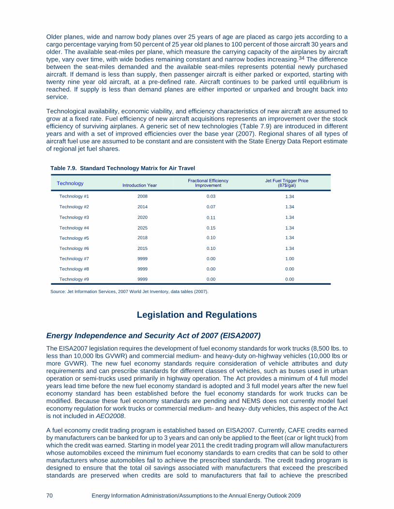
Older planes, wide and narrow body planes over 25 years of age are placed as cargo jets according to acargo percentage varying from 50 percent of 25 year old planes to 100 percent of those aircraft 30 years andolder. The available seat-miles per plane, which measure the carrying capacity of the airplanes by aircrafttype, vary over time, with wide bodies remaining constant and narrow bodies increasing.34 The differencebetween the seat-miles demanded and the available seat-miles represents potential newly purchasedaircraft. If demand is less than supply, then passenger aircraft is either parked or exported, starting withtwenty nine year old aircraft, at a pre-defined rate. Aircraft continues to be parked until equilibrium isreached. If supply is less than demand planes are either imported or unparked and brought back intoservice.
Technological availability, economic viability, and efficiency characteristics of new aircraft are assumed togrow at a fixed rate. Fuel efficiency of new aircraft acquisitions represents an improvement over the stockefficiency of surviving airplanes. A generic set of new technologies (Table 7.9) are introduced in differentyears and with a set of improved efficiencies over the base year (2007). Regional shares of all types ofaircraft fuel use are assumed to be constant and are consistent with the State Energy Data Report estimateof regional jet fuel shares.
Legislation and Regulations
Energy Independence and Security Act of 2007 (EISA2007)The EISA2007 legislation requires the development of fuel economy standards for work trucks (8,500 lbs. toless than 10,000 lbs GVWR) and commercial medium- and heavy-duty on-highway vehicles (10,000 lbs ormore GVWR). The new fuel economy standards require consideration of vehicle attributes and dutyrequirements and can prescribe standards for different classes of vehicles, such as buses used in urbanoperation or semi-trucks used primarily in highway operation. The Act provides a minimum of 4 full modelyears lead time before the new fuel economy standard is adopted and 3 full model years after the new fueleconomy standard has been established before the fuel economy standards for work trucks can bemodified. Because these fuel economy standards are pending and NEMS does not currently model fueleconomy regulation for work trucks or commercial medium- and heavy- duty vehicles, this aspect of the Actis not included in AEO2008.
A fuel economy credit trading program is established based on EISA2007. Currently, CAFE credits earnedby manufacturers can be banked for up to 3 years and can only be applied to the fleet (car or light truck) fromwhich the credit was earned. Starting in model year 2011 the credit trading program will allow manufacturerswhose automobiles exceed the minimum fuel economy standards to earn credits that can be sold to othermanufacturers whose automobiles fail to achieve the prescribed standards. The credit trading program isdesigned to ensure that the total oil savings associated with manufacturers that exceed the prescribedstandards are preserved when credits are sold to manufacturers that fail to achieve the prescribed
70 Energy Information Administration/Assumptions to the Annual Energy Outlook 2009
Technology Introduction YearFractional Efficiency
ImprovementJet Fuel Trigger Price
(87$/gal)
Technology #1 2008 0.03 1.34
Technology #2 2014 0.07 1.34
Technology #3 2020 0.11 1.34
Technology #4 2025 0.15 1.34
Technology #5 2018 0.10 1.34
Technology #6 2015 0.10 1.34
Technology #7 9999 0.00 1.00
Technology #8 9999 0.00 0.00
Technology #9 9999 0.00 0.00
Table 7.9. Standard Technology Matrix for Air Travel
Source: Jet Information Services, 2007 World Jet Inventory, data tables (2007).

standards. While the credit trading program begins in 2011, EISA2007 allows manufacturers to apply creditsearned to any of the 3 model years prior to the model year the credits are earned, and to any of the 5 modelyears after the credits are earned. The transfer of credits within a manufacturer’s fleet is limited to specificmaximums. For model years 2011 through 2013, the maximum transfer is 1.0 mpg; for model years 2014through 2017, the maximum transfer is 1.5 mpg; and for model years 2018 and later, the maximum credittransfer is 2.0 mpg. NEMS currently has a switch that allows for sensitivity analysis of CAFE credit bankingby manufacturer fleet, but does not model the trading of credits across manufacturers. The AEO2008 doesnot consider trading of credits since this would require significant modifications to NEMS and detailedtechnology cost and efficiency data by manufacturer, which is not readily available.
The CAFE credits specified under the Alternative Motor Fuels Act (AMFA) through 2019 is extended. Prior topassage of this Act, the CAFE credits under AMFA were scheduled to expire after model year 2010.Currently, 1.2 mpg is the maximum CAFE credit that can be earned from selling alternative fueled vehicles.EISA2007 extends the 1.2 mpg credit maximum through 2014 and reduces the maximum by 0.2 mpg foreach following year until it is phased out by model year 2020. NEMS does not model CAFE credits earnedfrom alternative fuel vehicles sales because manufacturer specific data would be required and althoughsome manufacturer detail is represented for light trucks, there is no manufacturer detail currentlyrepresented for cars. In addition, an algorithm that counts credits earned from the sale of alternative fueledvehicles would need to be added to NEMS, which would require significant modification to the modelstructure. AEO2008 does not consider this section of the Act.
Energy Improvement and Extension Act of 2008
EIEA2008 Title II, Section 205, provides a tax credit for the purchase of new, qualified plug-in electric drivemotor vehicles. According to the legislation, a qualified plug-in electric drive motor vehicle must drawpropulsion from a traction battery with at least 4 kilowatthours of capacity, use an off-board source of energyto recharge the battery, and, depending on the gross vehicle weight rating (GVWR), meet the EPA’s Tier IIvehicle emission standards or equivalent California low-emission vehicle emission standards.
The tax credit for the purchase of a plug-in electric vehicle is $2,500 plus $417 per kilowatthour of tractionbattery capacity in excess of the minimum required 4 kilowatthours, up to a total of $7,500 for a plug-in hybridvehicle with a GVWR of 10,000 pounds or less. The limit is raised to $10,000 for any new eligible plug-in witha GVWR between 10,000 and 14,000 pounds, $12,500 for a plug-in vehicle between 14,000 and 26,000pounds GVWR, and $15,000 for any eligible plug-in with a GVWR greater than 26,000 pounds.
The legislation also includes a phaseout period for the tax credit, beginning two calendar quarters after thefirst quarter in which the cumulative number of qualified plug-in electric vehicles sold in total by allmanufacturers reaches 250,000. The credit will be reduced by 50 percent in the first two calendar quarters ofthe phaseout period and by another 25 percent in the third and fourth calendar quarters. Thereafter, thecredit will be eliminated. Regardless of calendar quarter or whether 250,000 vehicles are sold, the credit willbe phased out after December 31, 2014. The tax credits for plug-in hybrid vehicles are included in AEO2009.
The Energy Policy Act of 2005
The Energy Policy Act of 2005 provides tax credits for the purchase of vehicles that have a lean burn engineor employ a hybrid or fuel cell propulsion system. The amount of the credit received for a vehicle is based thevehicle’s inertia weight, improvement in city tested fuel economy relative to an equivalent 2002 base yearvalue, emissions classification, and type of propulsion system. The tax credit is also sales limited bymanufacturer for vehicles with lean burn engines or hybrid propulsion systems. After December 31, 2005,the first calendar quarter a manufacturer’s sales of lean burn or hybrid vehicles reaches 60,000 units, thephase out period begins. Reduction of credits begins in the second calendar quarter following the initialquarter the sales maximum was reached. For that quarter and the following quarter, the applicable tax creditwill be reduced by 50 percent. For the subsequent third and fourth calendar quarters, the applicable taxcredit is reduced to 25 percent of the original value. These tax credits are included in the AEO2008.
Energy Policy Act of 1992 (EPACT)
Fleet alternative-fuel vehicle sales necessary to meet the EPACT regulations are derived based on themandates as they currently stand and the Commercial Fleet Vehicle Module calculations. Total projectedAFV sales are divided into fleets by government, business, and fuel providers (Table 7.10).
Energy Information Administration/Assumptions to the Annual Energy Outlook 2009 71

Because the commercial fleet model operates on three fleet type representations (business, government,and utility), the federal and state mandates are weighted by fleet vehicle stocks to create a compositemandate for both. The same combining methodology is used to create a composite mandate for electricutilities and fuel providers based on fleet vehicle stocks.35
Low Emission Vehicle Program (LEVP)The LEVP was originally passed into legislation in 1990 in the State of California. It began as theimplementation of a voluntary opt-in pilot program under the purview of Clean Air Act Amendments of 1990(CAAA90), which included a provision that other States could opt in to the California program to achievelower emissions levels than would otherwise be achieved through CAAA90. Twelve states have elected toadopt the California LEVP.
The LEVP is an emissions-based policy, setting sales mandates for 6 categories of low-emission vehicles:low-emission vehicles (LEVs), ultra-low-emission vehicles (ULEVs), super-ultra low emission vehicles(SULEVs), partial zero-emission vehicles (PZEVs), advanced technology partial zero emission vehicles(AT-PZEVs), and zero-emission vehicles (ZEVs). The LEVP requires that in 2005 10 percent of amanufacturer’s sales are ZEVs or equivalent ZEV earned credits, increasing to 11 percent in 2009, 12percent in 2012, 14 percent in 2015, and 16 percent in 2018 where it remains constant thereafter. In August2004, CARB enacted further amendments to the LEVP that place a greater emphasis on emissionsreductions from PZEVs and AT-PZEVs and requires that manufacturers produce a minimum number of fuelcell and electric vehicles. In addition, manufacturers are allowed to adopt alternative compliancerequirements for ZEV sales that are based on cumulative fuel cell vehicle sales targets for vehicles sold in allStates participating in California’s LEVP. Under the alternative compliance requirements, ZEV credits canalso be earned by selling battery electric vehicles. Currently, all manufacturers have opted to adhere to thealternative compliance requirements. The mandate still includes phase-in multipliers for pure ZEVs andallows 20 percent of the sales requirement to be met with AT-PZEVs and 60 percent of the requirement to bemet with PZEVs. AT-PZEVs and PZEVs are allowed 0.2 credits per vehicle. EIA assumes that creditallowances for PZEVs will be met with conventional vehicle technology, hybrid vehicles will be sold to meetthe AT-PZEV allowances, and that hydrogen fuel cell vehicles will be sold to meet the pure ZEVrequirements under the alternative compliance path.
Transportation Alternative Cases
High Technology CaseIn the high technology and low technology cases for cars and light trucks, the conventional fuel savingtechnology characteristics are based on NHTSA and EPA values.36 Tables 7.10, 7.11, 7.12, 7.13, and 7.14summarize the High and Low Technology matrices for cars and light trucks. Tables 7.15 and 7.16 reflect thehigh and low technology case assumptions for heavy trucks. These reflect optimistic and pessimistic values,with respect to efficiency improvement and capital cost, for advanced engine and emission controltechnologies as reported by ANL.37
For the Air Module, the high technology case reflects earlier introduction years for the new aircrafttechnologies and a greater penetration share. The low technology case is reflected by a delay in theintroduction of new aircraft technologies. Tables 7.17 and 7.18 reflect these cases.
72 Energy Information Administration/Assumptions to the Annual Energy Outlook 2009
Year Federal State Fuel Providers Electric Utilities2005 75 75 70 90
Table 7.10. EPACT Legislative Mandates for AFV Purchases by Fleet Type and Year(Percent)
Source: EIA, Energy Efficiency and Renewable Energy (Washington, DC, 2005), http://www1.eere.energy.gov/femp/about/fleet-requirements.html,http://www1.eere.energy.gov/vehicles and fuels/epact/state/state-gov.html.

Energy Information Administration/Assumptions to the Annual Energy Outlook 2009 73
Fractional Fuel
Efficiency Change
IncrementalCost
(1990$)
IncrementalCost
($/Unit Wt.)
Incremental Weight
(Lbs.)
IncrementalWeight
(Lbs./Unit Wt.)
Introduction Year
Fractional Horse-
power Change
Unit Body Construction 4 100 0 0 -6 1980 0Material Substitution II 3.3 0 0.4 0 -5 1990 0Material Substitution III 6.6 0 0.6 0 -10 1998 0Material Substitution IV 9.9 0 0.5 0 -15 2006 0Material Substitution V 13.2 0 1.1 0 -20 2014 0Drag Reduction II 1.6 16 0 0 0 1988 0Drag Reduction III 3.2 32 0 0 0.2 1992 0Drag Reduction IV 6.3 45 0 0 0.5 2000 0Drag Reduction V 8 53.5 0 0 1 2010 0Roll-Over Technology -1.5 100 0 0 2.2 2004 0Side Impact Technology -1.5 100 0 0 2.2 2004 0Adv Low Loss Torque Converter 2 25 0 0 0 1999 0Early Torque Converter Lockup 1 25.6 0 0 0 2002 0Aggressive Shift Logic 3.5 45 0 0 0 1999 04-Speed Automatic 4.5 285 0 10 0 1980 05-Speed Automatic 8 106.5 0 20 0 1995 06-Speed Automatic 5.5 103.8 0 30 0 2003 06-Speed Manual 2 91.4 0 20 0 1995 0CVT 6 213.9 0 -25 0 1998 0Automated Manual Trans 12 120.4 0 0 0 2004 0Roller Cam 2 16 0 0 0 1980 0OHC/AdvOHV-4 Cylinder 3 93.1 0 0 0 1980 10OHC/AdvOHV-6 Cylinder 3 108.9 0 0 0 1987 10OHC/AdvOHV-8 Cylinder 3 124.7 0 0 0 1986 104-Valve/4-Cylinder 8.8 205 0 10 0 1988 174-Valve/6-Cylinder 8.8 280 0 15 0 1992 174 Valve/8-Cylinder 8.8 320 0 20 0 1994 175 Valve/6-Cylinder 9 300 0 18 0 1998 20VVT-4 Cylinder 2.5 35 0 10 0 1994 5VVT-6 Cylinder 2.5 87.5 0 20 0 1993 5VVT-8 Cylinder 2.5 140 0 20 0 1993 5VVL-4 Cylinder 5 144.3 0 25 0 1997 10VVL-6 Cylinder 5 27.1 0 40 0 2000 10VVL-8 Cylinder 5 398 0 50 0 2000 10Camless Valve Actuation-4cyl 7.5 280 0 35 0 2020 13Camless Valve Actuation-6cyl 7.5 420 0 55 0 2020 13Camless Valve Actuation-8cyl 7.5 560 0 75 0 2020 13Cylinder Deactivation 6 173.4 0 10 0 2004 0Turbocharging/ Supercharging 5 295.1 0 -100 0 1980 15Engine Friction Reduction I 2 54 0 0 0 1992 3Engine Friction Reduction II 3.5 60.9 0 0 0 2000 5Engine Friction Reduction III 5 92.2 0 0 0 2008 7Engine Friction Reduction IV 6.5 177 0 0 0 2016 9Stoichiometric GDI/4-Cylinder 7 231.4 0 20 0 2006 10Stoichiometric GDI/6-Cylinder 7 311.3 0 30 0 2006 10Lean Burn GDI 6 640.5 0 20 0 2020 05W-30 Engine Oil 1 6.0 0 0 0 1998 05W-20 Engine Oil 2 37.5 0 0 0 2003 0OW-20 Engine Oil 3.1 150 0 0 0 2030 0Electric Power Steering 2 127.5 0 0 0 2004 0Improved Alternator 0.3 15 0 0 0 2005 0Improved Oil/Water Pump 0.5 10 0 0 0 2000 0Electric Oil/Water Pump 1 93.4 0 0 0 2007 0Tires II 2 6.1 0 -8 0 1995 0Tires III 3.5 12.3 0 -12 0 2005 0Tires IV 5 16.9 0 -16 0 2015 0Front Wheel Drive 6 250 0 0 -6 1980 0Four Wheel Drive Improvements 2 577.3 0 0 -1 2000 042V-Launch Assist and Regen 5 280 0 80 0 2005 -542V-Engine Off at Idle 7.5 496.6 0 45 0 2005 0Tier 2 Emissions Technology -1 120 0 20 0 2006 0Increased Size/Weight -1.7 0 0 0 2.55 2003 0Variable Compression Ratio 4 350 0 25 0 2015 0
Table 7.11. High Technology Matrix For Cars
Source: Energy and Environmental Analysis, Documentation of Technology included in the NEMS Fuel Economy Model for Passenger Cars and LightTrucks (September, 2002). National Research Council, Effectiveness and Impact of Corporate Average Fuel Economy (CAFE) Standards (Copyright2002). National Highway Traffic Safety Administration, Corporate Average Fuel Economy for MY 2011-2015 Passenger Cars and Light Trucks (April2008). U.S. Environmental Protection Agency, Interim Report: New Powertrain Technologies and Their Projected Costs (October 2005)
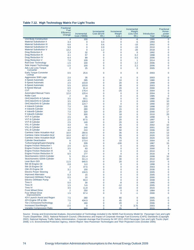
74 Energy Information Administration/Assumptions to the Annual Energy Outlook 2009
Fractional Fuel
Efficiency Change Incremental
Cost (1990$)
IncrementalCost ($/Unit
Wt.)
IncremenalWeight (Lbs.)
IncrementalWeight
(Lbs./Unit Wt.)
Introduction Year
Fractional Horse-
power Change
Unit Body Construction 4 100 0 0 -6 1980 0Material Substitution II 3.3 0 0.4 0 -5 1994 0Material Substitution III 6.6 0 0.6 0 -10 2002 0Material Substitution IV 9.9 0 0.9 0 -15 2010 0Material Substitution V 13.2 0 1.2 0 -20 2018 0Drag Reduction II 2.3 32 0 0 0 1992 0Drag Reduction III 4.1 57 0 0 0.2 1998 0Drag Reduction IV 6.4 89 0 0 0.5 2006 0Drag Reduction V 7.8 109 0 0 1 2014 0Roll-Over Technology -1.5 100 0 0 2.2 2006 0Side Impact Technology -1.5 100 0 0 2.2 2006 0Adv Low Loss Torque Converter
2 25 0 0 0 2005 0
Early Torque Converter Lockup
0.5 25.6 0 0 0 2003 0
Aggressive Shift Logic 2.0 35 0 0 0 2003 04-Speed Automatic 4.5 285 0 10 0 1980 05-Speed Automatic 2.5 103.8 0 20 0 1999 06-Speed Automatic 5.5 103.8 0 30 0 2003 06-Speed Manual 0.5 91.4 0 20 0 2000 0CVT 5.2 176.4 0 -25 0 2004 0Automated Manual Trans 12.0 120.4 0 0 0 2004 0Roller Cam 2 16 0 0 0 1985 0OHC/AdvOHV-4 Cylinder 3.5 93.1 0 0 0 1980 10OHC/AdvOHV-6 Cylinder 3.5 108.9 0 0 0 1990 10OHC/AdvOHV-8 Cylinder 3.5 124.7 0 0 0 1990 104-Valve/4-Cylinder 7.0 205 0 10 0 1998 174-Valve/6-Cylinder 7.0 280 0 15 0 2000 174 Valve/8-Cylinder 7.0 320 0 20 0 2000 175 Valve/6-Cylinder 7.0 300 0 18 0 2010 20VVT-4 Cylinder 2.5 35 0 10 0 1998 5VVT-6 Cylinder 2.5 87.5 0 20 0 1997 5VVT-8 Cylinder 2.5 140 0 20 0 1997 5VVL-4 Cylinder 4.0 70 0 25 0 2002 10VVL-6 Cylinder 4.0 140 0 40 0 2001 10VVL-8 Cylinder 4.0 210 0 50 0 2006 10Camless Valve Actuation-4cyl 10.0 284.6 0 35 0 2020 13Camless Valve Actuation-6cyl 10.0 427.2 0 55 0 2020 13Camless Valve Actuation-8cyll 10.0 569.8 0 75 0 2020 13Cylinder Deactivation 6 173.4 0 10 0 2004 0Turbocharging/Supercharging 6 339 0 -100 0 1987 15Engine Friction Reduction I 2.5 12.5 0 0 0 1992 3Engine Friction Reduction II 3.5 63 0 0 0 2000 5Engine Friction Reduction III 5 114 0 0 0 2010 7Engine Friction Reduction IV 6.5 177 0 0 0 2016 9Stoichiometric GDI/4-Cylinder 5 231.4 0 20 0 2008 10Stoichiometric GDI/6-Cylinder 5 311.3 0 30 0 2010 10Lean Burn GDI 11.5 640.5 0 20 0 2010 05W-30 Engine Oil 0.8 6.0 0 0 0 1998 05W-20 Engine Oil 2 37.5 0 0 0 2003 0OW-20 Engine Oil 3.1 150 0 0 0 2030 0Electric Power Steering 2 134.5 0 0 0 2005 0Improved Alternator 0.3 15 0 0 0 2005 0Improved Oil/Water Pump 0.5 10 0 0 0 2000 0Electric Oil/Water Pump 1 93.4 0 0 0 2008 0Tires II 0.0 30 0 -8 0 1995 0Tires III 1.5 5.6 0 -12 0 2005 0Tires IV 3.5 11.8 0 -16 0 2015 0Front Wheel Drive 2 250 0 0 -3 1984 0Four Wheel Drive Improvements
1.5 97.4 0 0 -1 2000 0
42V-Launch Assist and Regen 7.5 280 0 80 0 2005 -542V-Engine Off at Idle 7.5 434.9 0 45 0 2005 0Tier 2 EmissionsTechnology -1 160 0 20 0 2006 0Increased Size/Weight -2.5 0 0 0 3.75 2003 0Variable Compression Ratio 4 350 0 25 0 2015 0
Table 7.12. High Technology Matrix For Light Trucks
Source: Energy and Enviromental Analysis, Documentation of Technology included in the NEMS Fuel Economy Model for Passenger Cars and LightTrucks (September, 2002). National Research Council, Effectiveness and Impact of Corporate Average Fuel Economy (CAFE) Standards (Copyright2002). National Highway Traffic Safety Administration, Corporate Average Fuel Economy for MY 2011-2015 Passenger Cars and Light Trucks (April2008). U.S. Environmental Protection Agency, Interim Report: New Powertrain Technologies and Their Projected Costs (October 2005)

Energy Information Administration/Assumptions to the Annual Energy Outlook 2009 75
Fractional Fuel
Efficiency Change
IncrementalCost
(1990$)
Incremental Cost
($/Unit Wt.)
IncrementalWeight (Lbs.)
IncrementalWeight
(Lbs./UnitWt.)
Introduction Year
Fractional Horse-power
ChangeUnit Body Construction 4 100 0 0 -6 1980 0Material Substitution II 3.3 0 0.4 0 -5 1990 0Material Substitution III 6.6 0 0.6 0 -10 1998 0Material Substitution IV 9.9 0 0.9 0 -15 2006 0Material Substitution V 13.2 0 1.2 0 -20 2014 0Drag Reduction II 1.5 16.0 0 0 0 1988 0Drag Reduction III 3.0 32.0 0 0 0.2 1992 0Drag Reduction IV 4.2 45.0 0 0 0.5 2000 0Drag Reduction V 5.0 53.5 0 0 1 2010 0Roll-Over Technology -1.5 100 0 0 2.2 2004 0Side Impact Technology -1.5 100 0 0 2.2 2004 0Adv Low Loss Torque Converter
2 25 0 0 0 1999 0
Early Torque Converter Lockup
0.5 25.6 0 0 0 2002 0
Aggressive Shift Logic 1.7 45.0 0 0 0 1999 04-Speed Automatic 4.5 285 0 10 0 1980 05-Speed Automatic 2.5 106.5 0 20 0 1995 06-Speed Automatic 1.5 210.0 0 30 0 2003 06-Speed Manual 0.5 91.4 0 20 0 1995 0CVT 3.5 102.1 0 -25 0 1998 0Automated Manual Trans 4.0 175.0 0 0 0 2004 0Roller Cam 2 16 0 0 0 1980 0OHC/AdvOHV-4 Cylinder 3.5 105.0 0 0 0 1980 10OHC/AdvOHV-6 Cylinder 3.5 122.5 0 0 0 1987 10OHC/AdvOHV-8 Cylinder 3.5 140.0 0 0 0 1986 104-Valve/4-Cylinder 8 205 0 10 0 1988 174-Valve/6-Cylinder 8 280 0 15 0 1992 174 Valve/8-Cylinder 8 320 0 20 0 1994 175 Valve/6-Cylinder 8 300 0 18 0 1998 20VVT-4 Cylinder 2.5 50.4 0 10 0 1994 5VVT-6 Cylinder 2.5 114.4 0 20 0 1993 5VVT-8 Cylinder 2.5 178.5 0 20 0 1993 5VVL-4 Cylinder 2.0 70 0 25 0 1997 10VVL-6 Cylinder 2.0 140 0 40 0 2000 10VVL-8 Cylinder 2.0 210.0 0 50 0 2000 10Camless Valve Actuation-4cyl 2.5 286.9 0 35 0 2020 13Camless Valve Actuation-6cyl 2.5 430.8 0 55 0 2020 13Camless Valve Actuation-8cyl 2.5 574.7 0 75 0 2020 13Cylinder Deactivation 4.5 182 0 10 0 2004 0Turbocharging/Supercharging 6.1 455 0 -100 0 1980 15Engine Friction Reduction I 2.3 54 0 0 0 1992 3Engine Friction Reduction II 2.0 60.9 0 0 0 2000 5Engine Friction Reduction III 3.0 92.2 0 0 0 2008 7Engine Friction Reduction IV 6.5 177 0 0 0 2016 9Stoichiometric GDI/4-Cylinder 2.7 231.4 0 20 0 2006 10Stoichiometric GDI/6-Cylinder 2.7 311.3 0 30 0 2006 10Lean Burn GDI 10.0 640.5 0 20 0 2020 05W-30 Engine Oil 0.8 6.0 0 0 0 1998 05W-20 Engine Oil 2 37.5 0 0 0 2003 0OW-20 Engine Oil 3.1 150 0 0 0 2030 0Electric Power Steering 1.5 134.5 0 0 0 2004 0Improved Alternator 0.3 15 0 0 0 2005 0Improved Oil/Water Pump 0.5 10 0 0 0 2000 0Electric Oil/Water Pump 1 93.4 0 0 0 2007 0Tires II 1.5 35 0 -8 0 1995 0Tires III 1.5 35 0 -12 0 2005 0Tires IV 1.5 35 0 -16 0 2015 0Front Wheel Drive 6 250 0 0 -6 1980 0Four Wheel Drive Improvements
2 577.3 0 0 -1 2000 0
42V-Launch Assist and Regen 7.5 280 0 80 0 2005 -542V-Engine Off at Idle 5.5 496.6 0 45 0 2005 0Tier 2 Emissions Technology -1 120 0 20 0 2006 0Increased Size/Weight -1.7 0 0 0 2.55 2003 0Variable Compression Ratio 4 350 0 25 0 2015 0
Table 7.13. Low Technology Matrix For Cars1
1 Fractional changes refer to the percentage change from the 1990 values.Sources: Energy and Environment Analysis, Documentation of Technology included in the NEMS Fuel Economy Model for Passenger Cars and LightTrucks (September, 2002). National Research Council, Effectiveness and Impact of Corporate Average Fuel Economy (CAFE) Standards (Copyright2002). National Highway Traffic Safety Administration, Corporate Average Fuel Economy for MY 2011-2015 Passenger Cars and Light Trucks (April2008). U.S. Environmental Protection Agency, Interim Report: New Powertrain Technologies and Their Projected Costs (October 2005)

76 Energy Information Administration/Assumptions to the Annual Energy Outlook 2009
Fractional Fuel
Efficiency Change
IncrementalCost
(1990$)
Incremental Cost
($/UnitWt.)Incremental
Weight (Lbs.)
IncrementalWeight
(Lbs./UnitWt.)Introduction
Year
Fractional Horse-power
ChangeUnit Body Construction 4 100 0 0 -6 1980 0Material Substitution II 3.3 0 0.4 0 -5 1994 0Material Substitution III 6.6 0 0.6 0 -10 2002 0Material Substitution IV 9.9 0 0.9 0 -15 2010 0Material Substitution V 13.2 0 1.2 0 -20 2018 0Drag Reduction II 1.5 32 0 0 0 1992 0Drag Reduction III 4.1 57 0 0 0.2 1998 0Drag Reduction IV 6.4 89 0 0 0.5 2006 0Drag Reduction V 7.8 109 0 0 1 2014 0Roll-Over Technology -1.5 100 0 0 2.2 2006 0Side Impact Technology -1.5 100 0 0 2.2 2006 0Adv Low Loss Torque Converter 2 25 0 0 0 2005 0Early Torque Converter Lockup 0.5 25.6 0 0 0 2003 0Aggressive Shift Logic 1.5 32.5 0 0 0 2003 04-Speed Automatic 4.5 285 0 10 0 1980 05-Speed Automatic 2.5 112 0 20 0 1999 06-Speed Automatic 1.5 210 0 30 0 2003 06-Speed Manual 0.5 91.4 0 20 0 2000 0CVT 5.2 212.3 0 -25 0 2004 0Automated Manual Trans 4.0 175 0 0 0 2004 0Roller Cam 2 16 0 0 0 1985 0OHC/AdvOHV-4 Cylinder 3.5 105 0 0 0 1980 10OHC/AdvOHV-6 Cylinder 3.5 122.5 0 0 0 1990 10OHC/AdvOHV-8 Cylinder 3.5 140 0 0 0 1990 104-Valve/4-Cylinder 7 205 0 10 0 1998 174-Valve/6-Cylinder 7 280 0 15 0 2000 174 Valve/8-Cylinder 7 320 0 20 0 2000 175 Valve/6-Cylinder 7 300 0 18 0 2010 20VVT-4 Cylinder 2.5 101.6 0 10 0 1998 5VVT-6 Cylinder 2.5 140.1 0 20 0 1997 5VVT-8 Cylinder 2.5 178.5 0 20 0 1997 5VVL-4 Cylinder 2.8 210.1 0 25 0 2002 10VVL-6 Cylinder 2.8 322 0 40 0 2001 10VVL-8 Cylinder 2.8 433.8 0 50 0 2006 10Camless Valve Actuation-4cyl 2.5 284.6 0 35 0 2020 13Camless Valve Actuation-6cyl 2.5 427.2 0 55 0 2020 13Camless Valve Actuation-8cyl 2.5 569.8 0 75 0 2020 13Cylinder Deactivation 4.5 182 0 10 0 2004 0Turbocharging/Supercharging 6 650 0 -100 0 1987 15Engine Friction Reduction I 2.5 36 0 0 0 1992 3Engine Friction Reduction II 3.5 63 0 0 0 2000 5Engine Friction Reduction III 5 114 0 0 0 2010 7Engine Friction Reduction IV 6.5 177 0 0 0 2016 9Stoichiometric GDI/4-Cylinder 1.5 231.4 0 20 0 2008 10Stoichiometric GDI/6-Cylinder 1.5 311.3 0 30 0 2010 10Lean Burn GDI 10.0 640.5 0 20 0 2010 05W-30 Engine Oil 0.8 6.0 0 0 0 1998 05W-20 Engine Oil 2 37.5 0 0 0 2003 0OW-20 Engine Oil 3.1 150 0 0 0 2030 0Electric Power Steering 1.5 127.5 0 0 0 2005 0Improved Alternator 0.3 15 0 0 0 2005 0Improved Oil/Water Pump 0.5 10 0 0 0 2000 0Electric Oil/Water Pump 1 93.4 0 0 0 2008 0Tires II 0.0 30 0 -8 0 1995 0Tires III 1.0 35 0 -12 0 2005 0Tires IV 2.0 35 0 -16 0 2015 0Front Wheel Drive 2 250 0 0 -3 1984 0Four Wheel Drive Improvements
1.5 97.4 0 0 -1 2000 0
42V-Launch Assist and Regen 7.5 280 0 80 0 2005 -542V-Engine Off at Idle 5.5 434.9 0 45 0 2005 0Tier 2 Emissions Technology -1 160 0 20 0 2006 0Increased Size/Weight -2.5 0 0 0 3.75 2003 0Variable Compression Ratio 4 350 0 25 0 2015 0
Table 7.14. Low Technology Matrix For Light Trucks1
1Fractional changes refer to the percentage change from the 1990 values.Sources: Energy and Environment Analysis, Documentation of Technology included in the NEMS Fuel Economy Model for Passenger Cars and Light Trucks(September, 2002). National Research Council, Effectiveness and Impact of Corporate Average Fuel Economy (CAFE) Standards (Copyright 2002). NationalHighway Traffic Safety Administration, Corporate Average Fuel Economy for MY 2011-2015 Passenger Cars and Light Trucks (April 2008). U.S. EnvironmentalProtection Agency, Interim Report: New Powertrain Technologies and Their Projected Costs (October 2005)

Energy Information Administration/Assumptions to the Annual Energy Outlook 2009 77
Medium Light Trucks Medium Heavy Trucks Heavy Trucks
TechnologyType
Introd-uctionYear
Capital Cost
Incr.Fuel
Econ.Improve-
ment
Introd-uction Year
CapitalCost
Incr.Fuel
Econ.Improve-
ment
Introd-uction Year
Capital Cost
Incr.Fuel
Econ.Improve-
mentAreo dynamic I: Cab topdeflector,sloping hood and cabside flares
2002 600.00 0.028 0 750.00 0.028 0 750.00 0.028
Closing/covering of gapbetween tractor andtrailer, aero dynamicbumper, underside airbaffles, wheel wellcovers
N/A N/A 0.000 2004 800.00 0.041 2005 1500.00 0.023
Trailer leading andtrailing edge curvatures
N/A N/A 0.000 2005 400.00 0.013 2005 500.00 0.016
Aero Dynamics IV:pneumatic blowing
N/A N/A 0.000 N/A N/A 0.000 2010 2500.00 0.060
Tires I: radials 0 40.00 0.028 0 180.00 0.028 0 300.00 0.024
Tires II: low rollingresistance
2004 180.00 0.033 2005 280.00 0.033 2005 550.00 0.037
Tires III: super singles N/A N/A 0.000 N/A N/A 0.000 2008 700.00 0.028
Tires IV: reduced rollingresistance frompneumatic blowing
N/A N/A 0.000 N/A N/A 0.000 2015 500.00 0.011
Transmission: lock-up,electronic controls,reduced friction
2005 750.00 0.023 2005 900.00 0.023 2005 1000.00 0.023
Diesel Engine I:turbocharged, directinjection with betterthermal management
2003 600.00 0.045 2004 900.00 0.072 N/A N/A 0.000
Diesel Engine II:integratedstarter/alternator withidle off and limitedregenerative breaking
2005 1500.00 0.045 2005 1200.00 0.045 N/A N/A 0.000
Diesel Engine III:improved engine iwthlower friction, betterinjectors, and efficientcombustion
2012 2000.00 0.080 2008 2000.00 0.082 N/A 300.00 0.000
Diesel Engine IV: hybridelectric powertrain
2010 6000.00 0.360 2010 7000.00 0.360 N/A N/A 0.000
Diesel Engine V: internalfriction reduction -iimproved lubricants andbearings
N/A N/A 0.000 N/A N/A 0.000 2005 500.00 0.018
Diesel Engine VI:increased peak cylinderpressure
N/A NA 0.000 N/A N/A 0.000 2006 1000.00 0.036
Diesel Engine VII:improved injectors andmore efficientcombustion
N/A N/A 0.000 N/A N/A 0.000 2007 1500 0.054
Diesel Engine VIII:reduce waste heatimproved thermalmanagement
N/A N/A 0.000 N/A N/A 0.000 2010 2000 0.090
Table 7.15. High Technology Matrix for Freight Trucks

78 Energy Information Administration/Assumptions to the Annual Energy Outlook 2009
Medium Light Trucks Medium Heavy Trucks Heavy Trucks
TechnologyType Introd-
uctionYear
Capital Cost
Incr.Fuel
Econ.Improve-
ment
Introd-uction Year
CapitalCost
Incr.Fuel
Econ.Improve-
ment
Introd-uction Year
Capital Cost
Incr.Fuel
Econ.Improve-
mentGasoline Engine I:electronic fuelinjection, DOHC,multiple values
2003 700.00 0.045 2003 1000.00 0.045 N/A N/A 0.000
Gasoline Engine II:integratedstarter/alternator withidle off and limitedregenerative breaking
2005 1000.00 0.045 2005 1200.00 0.072 N/A N/A 0.000
Gasoline Engine III:direct injection (GDI)
2008 700.00 0.108 2008 1000.00 0.108 N/A N/A 0.000
Gasoline Engine IV;hybrid electricpowertrain
2010 6000.00 0.405 2010 8000.00 0.405 N/A N/A 0.000
Weight Reduction I:high strengthlightweight materials
2010 1300.00 0.045 2007 2000.00 0.045 2005 2000.00 0.090
Diesel Emission-NOxI: exhaustrecirculation, timingretard, selectivecatalytic reduction
2002 250.00 -0.030 2003 400.00 -0.030 2003 500.00 -0.030
Diesel Emissions-NOxII: nitrogen enrichedcombustion air
2003 500.00 -0.005 2003 700.00 -0.005 2003 750.00 -0.005
Diesel Emissions-NOxIII: non-thermalplasma catalyst
2007 1000.00 -0.010 2006 1200.00 -0.010 2007 1250.00 -0.010
Diesel Emissions-NOxIV: NOx absorbersystem
2007 1500.00 -0.020 2006 2000.00 -0.020 2007 2500.00 -0.020
Diesel Emission-PM I:oxidation catalyst
2002 150.00 -0.005 2002 200.00 -0.005 2002 250.00 -0.005
Diesel Emission-PMII: catalytic particulatefilter
2006 1000.00 -0.010 2006 1250.00 -0.020 2006 1500.00 -0.010
Diesel Emission-HC/CO I: oxidationcatalyst
2002 150.00 -0.005 2002 200.00 -0.005 2002 250.00 -0.005
Diesl Emission-HC/CO II: closedcrankcase system
2005 50.00 0.000 2005 65.00 0.000 2005 75.00 0.000
Gasoline Emission-PM I: Improvedoxidation catalyst
2005 250.00 -0.003 2005 350.00 -0.003 N/A N/A 0.000
GasolineEmission-NOx I:EGR/spark retard
2002 25.00 -0.010 2002 25.00 -0.010 N/A N/A 0.000
GasolineEmission-NOx II:oxygen sensors
2003 75.00 0.000 2003 75.00 0.000 N/A N/A 0.000
GasolineEmission-NOx III:secondary air/closedloop system
2008 50.00 0.000 2008 50.00 0.000 N/A N/A 0.000
Table 7.15. High Technology Matrix for Freight Trucks (cont.)

Energy Information Administration/Assumptions to the Annual Energy Outlook 2009 79
Medium Light Trucks Medium Heavy Trucks Heavy Trucks
TechnologyType
Introd-uctionYear
Capital Cost
Incr.Fuel
Econ.Improve-
ment
Introd-uction Year
CapitalCost
Incr.Fuel
Econ.Improve-
ment
Introd-uction Year
Capital Cost
Incr.Fuel
Econ.Improve-
mentGasoline Emission-HC/CO I: oxygensensors 2003 75.00 0.000 2003 75.00 0.000 N/A N/A 0.000
Gasoline Emission-HC/CO II: evap.canister w/improvedvaccum, materials,and connectors
2003 50.00 0.000 2003 50.00 0.000 N/A N/A 0.000
Gasoline Emission-HC/CO III: oxidationcatalyst
2005 250.00 -0.003 2005 350.00 -0.003 N/A N/A 0.000
1. Payback period is same for the three modes.
Table 7.15. High Technology Matrix for Freight Trucks (cont.)

80 Energy Information Administration/Assumptions to the Annual Energy Outlook 2009
Medium Light Trucks Medium Heavy Trucks Heavy Trucks
TechnologyType
Introd-uctionYear
Capital Cost
Incr.Fuel
Econ.Improve-
ment
Introd-uction Year
CapitalCost
Incr.Fuel
Econ.Improve-
ment
Introd-uction Year
Capital Cost
Incr.Fuel
Econ.Improve-
mentAreo dynamic I: Cab topdeflector,sloping hood and cabside flares
2002 600.00 0.018 0 750.00 0.018 0 750.00 0.013
Closing/covering of gapbetween tractor andtrailer, aero dynamicbumper, underside airbaffles, wheel wellcovers
N/A N/A 0.000 2004 800.00 0.031 2005 1500.00 0.023
Trailer leading andtrailing edge curvatures
N/A N/A 0.000 2005 400.00 0.005 2005 500.00 0.008
Aero Dynamics IV:pneumatic blowing
N/A N/A 0.000 N/A N/A 0.000 2010 2500.00 0.030
Tires I: radials 0 40.00 0.008 0 180.00 0.008 0 300.00 0.004
Tires II: low rollingresistance
2004 180.00 0.013 2005 280.00 0.033 2005 550.00 0.017
Tires III: super singles N/A N/A 0.000 N/A N/A 0.000 2008 700.00 0.008
Tires IV: reduced rollingresistance frompneumatic blowing
N/A N/A 0.000 N/A N/A 0.000 2015 500.00 0.011
Transmission: lock-up,electronic controls,reduced friction
2005 750.00 0.013 2005 900.00 0.013 2005 1000.00 0.013
Diesel Engine I:turbocharged, directinjection with betterthermal management
2003 800.00 0.045 2004 1100.00 0.072 N/A N/A 0.000
Diesel Engine II:integratedstarter/alternator withidle off and limitedregenerative breaking
2005 1500.00 0.045 2005 1200.00 0.045 N/A N/A 0.000
Diesel Engine III:improved engine iwthlower friction, betterinjectors, and efficientcombustion
2012 2000.00 0.070 2008 2000.00 0.062 N/A 300.00 0.000
Diesel Engine IV: hybridelectric powertrain
2010 6000.00 0.360 2010 9000.00 0.360 N/A N/A 0.000
Diesel Engine V: internalfriction reduction -iimproved lubricants andbearings
N/A N/A 0.000 N/A N/A 0.000 2005 500.00 0.018
Diesel Engine VI:increased peak cylinderpressure
N/A NA 0.000 N/A N/A 0.000 2006 1000.00 0.036
Diesel Engine VII:improved injectors andmore efficientcombustion
N/A N/A 0.000 N/A N/A 0.000 2007 1500 0.054
Diesel Engine VIII:reduce waste heatimproved thermalmanagement
N/A N/A 0.000 N/A N/A 0.000 2010 2000 0.090
Table 7.16. Low Technology Matrix for Freight Trucks

Energy Information Administration/Assumptions to the Annual Energy Outlook 2009 81
Medium Light Trucks Medium Heavy Trucks Heavy Trucks
TechnologyType Introd-
uctionYear
Capital Cost
Incr.Fuel
Econ.Improve-
ment
Introd-uction Year
CapitalCost
Incr.Fuel
Econ.Improve-
ment
Introd-uction Year
Capital Cost
Incr.Fuel
Econ.Improve-
mentGasoline Engine I:electronic fuelinjection, DOHC,multiple values
2003 700.00 0.045 2003 1000.00 0.045 N/A N/A 0.000
Gasoline Engine II:integratedstarter/alternator withidle off and limitedregenerative breaking
2005 1000.00 0.045 2005 1200.00 0.072 N/A N/A 0.000
Gasoline Engine III:direct injection (GDI)
2008 700.00 0.108 2008 1000.00 0.108 N/A N/A 0.000
Gasoline Engine IV;hybrid electricpowertrain
2010 6000.00 0.405 2010 8000.00 0.405 N/A N/A 0.000
Weight Reduction I:high strengthlightweight materials
2010 1300.00 0.045 2007 2000.00 0.045 2005 2000.00 0.090
Diesel Emission-NOxI: exhaustrecirculation, timingretard, selectivecatalytic reduction
2002 250.00 -0.050 2003 400.00 -0.050 2003 500.00 -0.050
Diesel Emissions-NOxII: nitrogen enrichedcombustion air
2003 500.00 -0.005 2003 700.00 -0.005 2003 750.00 -0.005
Diesel Emissions-NOxIII: non-thermalplasma catalyst
2007 1000.00 -0.020 2006 1200.00 -0.020 2007 1250.00 -0.020
Diesel Emissions-NOxIV: NOx absorbersystem
2007 1500.00 -0.040 2006 2000.00 -0.040 2007 2500.00 -0.040
Diesel Emission-PM I:oxidation catalyst
2002 150.00 -0.005 2002 200.00 -0.005 2002 250.00 -0.005
Diesel Emission-PMII: catalytic particulatefilter
2006 1000.00 -0.020 2006 1250.00 -0.030 2006 1500.00 -0.020
Diesel Emission-HC/CO I: oxidationcatalyst
2002 150.00 -0.005 2002 200.00 -0.005 2002 250.00 -0.005
Diesl Emission-HC/CO II: closedcrankcase system
2005 50.00 0.000 2005 65.00 0.000 2005 75.00 0.000
Gasoline Emission-PM I: Improvedoxidation catalyst
2005 250.00 -0.003 2005 350.00 -0.003 N/A N/A 0.000
GasolineEmission-NOx I:EGR/spark retard
2002 25.00 -0.020 2002 25.00 -0.020 N/A N/A 0.000
GasolineEmission-NOx II:oxygen sensors
2003 75.00 0.000 2003 75.00 0.000 N/A N/A 0.000
GasolineEmission-NOx III:secondary air/closedloop system
2008 50.00 0.000 2008 50.00 0.000 N/A N/A 0.000
Table 7.16. Low Technology Matrix for Freight Trucks (cont.)

82 Energy Information Administration/Assumptions to the Annual Energy Outlook 2009
Medium Light Trucks Medium Heavy Trucks Heavy Trucks
TechnologyType
Introd-uctionYear
Capital Cost
Incr.Fuel
Econ.Improve-
ment
Introd-uction Year
CapitalCost
Incr.Fuel
Econ.Improve-
ment
Introd-uction Year
Capital Cost
Incr.Fuel
Econ.Improve-
mentGasoline Emission-HC/CO I: oxygensensors 2003 75.00 0.000 2003 75.00 0.000 N/A N/A 0.000
Gasoline Emission-HC/CO II: evap.canister w/improvedvaccum, materials,and connectors
2003 50.00 0.000 2003 50.00 0.000 N/A N/A 0.000
Gasoline Emission-HC/CO III: oxidationcatalyst
2005 250.00 -0.003 2005 350.00 -0.003 N/A N/A 0.000
1. Payback period is same for the three modes.
Table 7.16. Low Technology Matrix for Freight Trucks (cont.)

Energy Information Administration/Assumptions to the Annual Energy Outlook 2009 83
Technology Introduction YearFractional Efficiency
ImprovementJet Fuel Trigger Price
(87$/gal)
Technology #1 2008 0.03 1.34
Technology #2 2008 0.07 1.34
Technology #3 2015 0.11 1.34
Technology #4 2020 0.15 1.34
Technology #5 2018 0.22 1.34
Technology #6 2018 0.10 1.34
Technology #7 2025 0.00 1.00
Technology #8 2020 0.10 0.00
Technology #9 9999 0.00 0.00
Table 7.17. High Technology Matrix for Air Travel
Source: Jet Information Services, 2007 World Jet Inventory, data tables (2007). Energy Information Administration, Transportation SectorModel of the National Energy Modeling System, Model Documentation 2008, DOE/EIA-M070(2008), (Washington, DC, 2008).
Technology Introduction YearFractional Efficiency
ImprovementJet Fuel Trigger Price
(87$/gal)
Technology #1 2008 0.03 1.34
Technology #2 2019 0.07 1.34
Technology #3 2025 0.11 1.34
Technology #4 9999 0.00 1.34
Technology #5 2018 0.10 1.34
Technology #6 2018 0.10 1.34
Technology #7 9999 0.00 1.00
Technology #8 9999 0.00 0.00
Technology #9 9999 0.00 0.00
Table 7.18. Low Technology Matrix for Air Travel
Source: et Information Services, 2007 World Jet Inventory, data tables (2007). Energy Information Administration, Transportation SectorModel of the National Energy Modeling System, Model Documentation 2008, DOE/EIA-M070(2008), (Washington, DC, 2008).

[1] U.S. Department of Transportation, National Highway Traffic and Safety Administration, “Summary ofFuel Economy Performance”, (Washington, DC, March 2004).
[2] Goldberg, Pinelopi Koujianou, “Product Differentiation and Oligopoly In International Markets: The Caseof The U.S. Automobile Industry,” Econometrica, Vol. 63, No.4 (July, 1995), 891-951.
[3] Oak Ridge National Laboratory, “Fleet Characteristics And Data Issues,” Davis, Stacy C, Lorena Truett,Oak Ridge National Laboratory, (Oak Ridge, TN, january 2003).
[4] Bobit Publishing Company, The Fleet Fact Book, various issues (Redondo Beech, California).
[5] Bobit Publishing Company, Note 4.
[6] Davis, Stacy C., Lorena F. Truett, “Investigation of Class 2B Trucks (Vehicles of 8,500 to 10,000 LBSGVWR),” Oak Ridge National Laboratory, ORNL/TM-2002/49, March 2002.
[7] Davis, Stacy C., Lorena F. Truett, op.cit., Note 6.
[8] Greenspan, Alan, and Darrel Cohen, “Motor Vehicle Stocks, Scrappage, and Sales,” Federal ReserveBoard (Washington, DC, October 30, 1996).
[9] Oak Ridge National Laboratory, Transportation Energy Data Book: 27 and Annual (Oak Ridge, TN,2008).
[10] Davis, Stacy C., Lorena F. Truett, op.cit., Note 6.
[11] Greene, David L. and S.M. Chin, “Alternative Fuels and Vehicles (AFV) Model Changes,” Center forTransportation Analysis, Oak Ridge National Laboratory, (Oak Ridge, TN, November 14, 2000).
[12] U.S. Department of Energy, Office of Energy Efficiency and Renewable Energy, prepared byInterlaboratory Working Group, Scenarios of U.S. Carbon Reductions: Potential Impacts of EnergyTechnologies by 2010 and Beyond, (Washington, DC, 1998).
[13] Energy and Environmental Analysis, Inc., Updates to the Fuel Economy Model (FEM) and AdvancedTechnology Vehicle (ATV) Module of the National Energy Modeling System (NEMS) Transportation Model,Prepared for the Energy Information Administration (EIA), (Arlington, VA, October 23, 2000).
[14] Energy Information Administration, Alternatives to Traditional Transportation Fuels 2005,hhttp://www.eia.doe.gov/cneaf/alternate/page/aftables/afvtransfuel_II.html #in use.
[15] Energy Information Administration, State Energy Data 2005 Consumption as downloaded July 2008,from http://www.eia.doe.gov/emeu/states/_Seds.html.
[16] Decision Analysis Corporation of Virginia, “Re-estimation of Freight Adjustment Coefficients,” Reportprepared for the Energy Information Administration (EIA), February 28, 1995).
[17] Reebie Associates, TRANSEARCH Freight Commodity Flow Database, (Greenwich, CT, 1992).
[18] U.S. Department of Commerce, Bureau of Census, Vehicle Inventory and Use Survey, EC97TV,(Washington, DC, October 1999).
[19] Vyas, A., C. Saricks, and F. Stodolsky, “The Potential Effect of Future Energy Efficiency andEmissions Improving Technology on Fuel Consumption of Heavy Trucks,” Argonne National Laboratory,(Argonne, IL, 2002).
[20] Davis, Stacy C., “Memorandum on the Distribution of Trucks by Age and Weight: 2000 TruckPopulation,” Oak Ridge National Laboratory, (Oak Ridge, TN, November 2001)
84 Energy Information Administration/Assumptions to the Annual Energy Outlook 2009
Notes and Sources

[21] Davis, Stacy C., op. cit., Note 20.
[22] Schmoyer, Rick, “Scrappage of Heavy Trucks - Estimates for the Year 2000,” Oak Ridge NationalLaboratory, DRAFT, (Oak Ridge, TN, June 2001).
[23] Decision Analysis Corporation of Virginia, op. cit. Note 19.
[24] Reebie Associates, op. cit., Note 17.
[25] Oak Ridge National Laboratory, Op. cit. Note 9.
[26] U.S. Department of Transportation, Federal Railroad Administration, “1989 Carload WaybillStatistics; Territorial Distribution, Traffic and Revenue by Commodity Classes,” (September 1991 and Priorissues).
[27] Energy Information Administration, op. cit., Note 15.
[28] Army Corps of Engineers, Waterborne Commerce of the United States, (Waterborne Statistics Center:New Orleans, LA, 1993).
[29] Energy Information Administration, op. cit., Note 15.
[30] Bureau of Transportation Statistics, Office of Airline Information, Air Carrier Summary Data (Form 41,Schedules T-1 and T-2), (2007). http://www.transtats.bts.gov/DataIndex.asp; link: Air Carrier Summary Data(Form 41 and 298C Summary Data).
[31] Bureau of Transportation Statistics, op. cit., Note 30.
[32] U.S. Department of Transportation, Federal Aviation Administration, Airport Capacity BenchmarkReport, 2004 (2004).
[33] Jet Information Services Inc., World Jet Inventory: Year-End 2007, (December 2007).
[34] Bureau of Transportation Statistics, op. cit., Note 30.
[35] Energy Information Administration, op. cit. Note 14
[36] Energy and Environmental Analysis, Inc., “Documentation of Technologies Included in the NEMS FuelEconomy Model for Passenger Cars and Light Trucks,” Prepared for the Energy Information Administration,(Arlington, VA, September 30, 2002).
[37] Vyas, A., C. Saricks, and F. Stodolsky, “Projected Effect of Future Efficiency and EmissionsImproving Technologies on Fuel Consumption of Heavy Trucks,” Argonne National Laboratory, (Argonne,IL, 2001).
Energy Information Administration/Assumptions to the Annual Energy Outlook 2009 85
Notes and Sources


Electricity Market ModuleThe NEMS Electricity Market Module (EMM) represents the capacity planning, dispatching, and pricing ofelectricity. It is composed of four submodules—electricity capacity planning, electricity fuel dispatching, loadand demand electricity, and electricity finance and pricing. It includes nonutility capacity and generation, andelectricity transmission and trade. A detailed description of the EMM is provided in the EIA publication,Electricity Market Module of the National Energy Modeling System 2009, DOE/EIA-M068(2009).
Based on fuel prices and electricity demands provided by the other modules of the NEMS, the EMMdetermines the most economical way to supply electricity, within environmental and operational constraints.There are assumptions about the operations of the electricity sector and the costs of various options in eachof the EMM submodules. This section describes the model parameters and assumptions used in EMM. Itincludes a discussion of legislation and regulations that are incorporated in EMM as well as informationabout the climate change action plan. The various electricity and technology cases are also described.
EMM Regions
The supply regions used in EMM are based on the North American Electric Reliability Council regions andsubregions shown in Figure 6 (region definitions as of 2004).
Energy Information Administration/Assumptions to the Annual Energy Outlook 2009 87
11
13
12
5
2
10
8
9
4 13
6
7
Figure 6. Electricity Market Model Supply Regions
1 East Central Area Reliability Coordination Agreement (ECAR) 8 Florida Reliability Coordinating Council (FL) 2 Electric Reliability Council of Texas (ERCOT) 9 Southeastern Electric Reliability Council (SERC) 3 Mid-Atlantic Area Council (MAAC) 10 Southwest Power Pool (SPP) 4 Mid-America Interconnected Network (MAIN) 11 Northwest Power Pool (NWP) 5 Mid-Continent Area Power Pool (MAPP) 12. Rocky Mountain Power Area, Arizona, New Mexico, and 6. New York (NY) Southern Nevada (RA) 7. New England (NE) 13 California (CA)
Report #:DOE/EIA-0554(2009)
Release date: March 2009
Next release date: March 2010

Model Parameters and Assumptions
Generating Capacity TypesThe capacity types represented in the EMM are shown in Table 8.1.
New Generating Plant CharacteristicsThe cost and performance characteristics of new generating technologies are inputs to the electricitycapacity planning submodule (Table 8.2). These characteristics are used in combination with fuel pricesfrom the NEMS fuel supply modules and foresight on fuel prices, to compare options when new capacity isneeded. Heat rates for fossil-fueled technologies are assumed to decline linearly through 2025.
The overnight costs shown in Table 8.2 are the cost estimates to build a plant in a typical region of thecountry. Differences in plant costs due to regional distinctions are calculated by applying regional multipliersthat represent variations in the cost of labor. The base overnight cost is multiplied by a project contingencyfactor and a technological optimism factor (described later in this chapter), resulting in the total constructioncost for the first-of-a-kind unit used for the capacity choice decision.
The base overnight costs for AEO2009 were updated to reflect current costs and capture some of the rapidincreases due to rising comodity costs. A new cost adjustment factor was also implemented based on theproducer price index for metals and metal products, allowing the overnight costs to fall in the future if thisindex drops, or rise further if it increases.
88 Energy Information Administration/Assumptions to the Annual Energy Outlook 2009
Capacity Type
Existing coal steam plants1
High Sulfur Pulverized Coal with Wet Flue Gas DesulfurizationAdvanced Coal - Integrated Coal Gasification Combined CycleAdvanced Coal with carbon sequestrationOil/Gas Steam - Oil/Gas Steam TurbineCombined Cycle - Conventional Gas/Oil Combined Cycle Combustion TurbineAdvanced Combined Cycle - Advanced Gas/Oil Combined Cycle Combustion TurbineAdvanced Combined Cycle with carbon sequestrationCombustion Turbine - Conventional Combustion TurbineAdvanced Combustion Turbine - Steam Injected Gas TurbineMolten Carbonate Fuel Cell
Conventional NuclearAdvanced Nuclear - Advanced Light Water ReactorGeneric Distributed Generation - BaseloadGeneric Distributed Generation - PeakConventional Hydropower - Hydraulic TurbinePumped Storage - Hydraulic Turbine ReversibleGeothermalMunicipal Solid WasteBiomass - Integrated Gasification Combined-CycleSolar Thermal - Central ReceiverSolar Photovoltaic - Single Axis Flat PlateWindWind Offshore
Table 8.1. Generating Capacity Types Represented in the Electricity Market Module
1The EMM represents 32 different types of existing coal steam plants, based on the different possible configuration of Nox,particulate and SO2 emission control devices, as well as future options for controlling mercury.
Source: Energy Information Administration, Office of Integrated Analysis and Forecasting.

Energy Information Administration/Assumptions to the Annual Energy Outlook 2009 89
TechnologyOnline
Year1Size(mW)
Leadtime(Years)
BaseOvernight
Costin 2008
($2007/kW)
Contingency Factors
Project Technological Contingency Optimism
Factor2 Factor3
TotalOvernight
Cost in 20084
(2007 $/kW)
VariableO&M5
($2007 mills/kWh)
FixedO&M5
($2007/kW)
Heatrate6
in 2008
(Btu/kWhr)
Heatrate nth-of- a-kind
(Btu/kWr)
Scrubbed Coal New7 20121 600 4 1,923 1.07 1.00 2,058 4.59 27.53 9,200 8,740
Integrated Coal-Gasification Combined Cycle (IGCC)7 2012 550 4 2,223 1.07 1.00 2,378 2.92 38.67 8,765 7,450
IGCC with Carbon Sequestration 2016 380 4 3,172 1.07 1.03 3,496 4.44 46.12 10,781 8,307
Conv Gas/Oil Comb Cycle 2011 250 3 917 1.05 1.00 962 2.07 12.48 7,196 6,800
Adv Gas/Oil Comb Cycle (CC) 2011 400 3 877 1.08 1.00 948 2.00 11.70 6,752 6,333
ADV CC with Carbon Sequestration 2016 400 3 1,683 1.08 1.04 1,890 2.94 19.90 8,613 7,493
Conv Combustion Turbine8 2010 160 2 638 1.05 1.00 670 3.57 12.11 10,810 10,450
Adv Combustion Turbine 2010 230 2 604 1.05 1.00 634 3.17 10.53 9,289 8,550
Fuel Cells 2011 10 3 4,640 1.05 1.10 5,360 47.92 5.65 7,930 6,960
Advanced Nuclear 2016 1350 6 2,873 1.10 1.05 3,318 0.49 90.02 10,434 10,434
Distributed Generation -Base 2011 2 3 1,305 1.05 1.00 1,370 7.12 16.03 9,050 8,900
Distributed Generation -Peak 2010 1 2 1,566 1.05 1.00 1,645 7.12 16.03 10,069 9,880
Biomass 2012 80 4 3,339 1.07 1.05 3,766 6.71 64.45 9,646 7,765
MSW - Landfill Gas 2010 30 3 2,377 1.07 1.00 2,543 0.01 114.25 13,648 13,648
Geothermal 7,9 2010 50 4 1,630 1.05 1.00 1,711 0.00 164.64 34,633 30,301
Conventional Hydropower9 2012 500 4 2,038 1.10 1.00 2,242 2.43 13.63 9,919 9,919
Wind 2009 50 3 1,797 1.07 1.00 1,923 0.00 30.30 9,919 9,919
Wind Offshore 2012 100 4 3,416 1.10 1.03 3,851 0.00 89.48 9,919 9,919
Solar Thermal7 2012 100 3 4,693 1.07 1.00 5,021 0.00 56.78 9,919 9,919
Photovoltaic7 2011 5 2 5,750 1.05 1.00 6,038 0.00 11.68 9,919 9,919
Table 8.2. Cost and Performance Characteristics of New Central Station Electricity Generating Technologies
1Online year represents the first year that a new unit could be completed, given an order date of 2008. For wind, geothermal andlandfill gas, the online year was moved earlier to acknowledge the significant market activity already occuring in anticipation of theexpiration of the Production Tax Credit in 2009 for wind and 2010 for the others.2A contingency allowance is defined by the American Association of Cost Engineers as the "specific provision for unforeseeableelements if costs within a defined project scope; particularly important where previous experience has shown that unforeseeableevents which will increase costs are likely to occur."3The technological optimism factor is applied to the first four units of a new, unproven design. It reflects the demonstrated tendencyto underestimate actual costs for a first-of-a-kind unit.4Overnight capital cost including contingency factors, excluding regional multipliers and learning effects. Interest charges are alsoexcluded. These represent costs of new projects initiated in 2008.5O&M = Operations and maintenance.6For hydro, wind, and solar technologies, the heatrate shown represents the average heatrate for conventional thermal generationas of 2007. This is used for purposes of calculating primary energy consumption displaced for these resources, and does not implyan estimate of their actual energy conversion efficiency.7Capital costs are shown before investment tax credits are applied.8Combustion turbine units can be built by the model prior to 2010 if necessary to meet a given region's reserve margin.9Because geothermal and hydro cost and performance characteristics are specific for each site, the table entries represent the costof the least expensive plant that could be built in the Northwest Power Pool region, where most of the proposed sites are located.
Sources: The values shown in this table are developed by the Energy Information Administration, Office of Integrated Analysis andForecasting, from analysis of reports and discussions with various sources from industry, government, and the Department ofEnergy Fuel Offices and National Laboratories. They are not based on any specific technology model, but rather, are meant torepresent the cost and performance of typical plants under normal operating conditions for each plant type. Key sources reviewedare listed in the ‘Notes and Sources’ section at the end of the chapter.

Technological Optimism and LearningOvernight costs for each technology are calculated as a function of regional construction parameters, projectcontingency, and technological optimism and learning factors.
The technological optimism factor represents the demonstrated tendency to underestimate actual costs for afirst-of-a-kind, unproven technology. As experience is gained (after building 4 units) the technologicaloptimism factor is gradually reduced to 1.0.
The learning function in NEMS is determined at a component level. Each new technology is broken into itsmajor components, and each component is identified as revolutionary, evolutionary or mature. Differentlearning rates are assumed for each component, based on the level of experience with the designcomponent (Table 8.3). Where technologies use similar components, these components learn at the samerate as these units are built. For example, it is assumed that the underlying turbine generator for acombustion turbine, combined cycle and integrated coal-gasification combined cycle unit is basically thesame. Therefore construction of any of these technologies would contribute to learning reductions for theturbine component.
The learning function has the nonlinear form:
OC(C) = a*C-b,
where C is the cumulative capacity for the technology component.
90 Energy Information Administration/Assumptions to the Annual Energy Outlook 2009
Period 1 Period 2 Period 3 Period 1 Period 2 Minimum Total
Technology Component LearningRate
LearningRate
LearningRate
Doublings Doublings Learning by 2025
Pulverized Coal - - 1% - - 5%
Combustion Turbine - conventional - - 1% - - 5%
Combustion Turbine - advanced - 10% 1% - 5 10%
HRSG1 - - 1% - - 5%
Gasifier - 10% 1% - 5 10%
Carbon Capture/Sequestration 20% 10% 1% 3 5 20%
Balance of Plant - IGCC - - 1% - - 5%
Balance of Plant - Turbine - - 1% - - 5%
Balance of Plant - Combined Cycle - - 1% - - 5%
Fuel Cell 20% 10% 1% 3 5 20%
Advanced Nuclear 5% 3% 1% 3 5 10%
Fuel prep - Biomass IGCC 20% 10% 1% 3 5 20%
Distributed Generation - Base - 5% 1% - 5 10%
Distributed Generation - Peak - 5% 1% - 5 10%
Geothermal - 8% 1% - 5 10%
Municipal Solid Waste - - 1% - - 5%
Hydropower - - 1% - - 5%
Wind - - 1% - - 1%
Wind Offshore 20% 10% 1% 3 5 20%
Solar Thermal 20% 10% 1% 3 5 20%
Solar PV 15% 8% 1% 3 5 20%
Table 8.3. Learning Parameters for New Generating Technology Components
1HRSG = Heat Recovery Steam Generator
Note: Please see the text for a description of the methodology for learning in the Electricity Market Module.
Source: Energy Information Administration, Office of Integrated Analysis and Forecasting.

The progress ratio (pr) is defined by speed of learning (e.g., how much costs decline for every doubling ofcapacity). The reduction in capital cost for every doubling of cumulative capacity (f) is an exogenousparameter input for each component (Table 8.3). Consequently, the progress ratio and f are related by:
pr = 2-b = (1 - f)
The parameter “b” is calculated by (b =-(ln(1-f)/ln(2)). The parameter “a” can be found from initial conditions.That is,
a =OC(C0)/C0-b
where C0 is the cumulative initial capacity. Thus, once the rates of learning (f) and the cumulative capacity(C0) are known for each interval, the corresponding parameters (a and b) of the nonlinear function areknown. Three learning steps were developed, to reflect different stages of learning as a new design isintroduced to the market. New designs with a significant amount of untested technology will see high rates oflearning initially, while more conventional designs will not have as much learning potential. All designcomponents receive a minimal amount of learning, even if new capacity additions are not projected. Thisrepresents cost reductions due to future international development or increased research and development.
Once the learning rate by component is calculated, a weighted average learning factor is calculated for eachtechnology. The weights are based on the share of the initial cost estimate that is attributable to eachcomponent (Table 8.4). For technologies that do not share components, this weighted average learning rateis calculated exogenously, and input as a single component. These technologies may still have a mix ofrevolutionary components and more mature components, but it is not necessary to include this detail in themodel unless capacity from multiple technologies would contribute to the component learning.
Table 8.5 shows the capacity credit toward component learning for the various technologies. It was assumedthat for all combined-cycle technologies, the turbine unit contributed two-thirds of the capacity, and thesteam unit one-third. Therefore, building one gigawatt of gas combined cycle would contribute 0.67gigawatts toward turbine learning, and 0.33 gigawatts toward steam learning. All non-capacity components,such as the balance of plant category, contribute 100 percent toward the component learning.
International Learning. In AEO2009, capital costs for all new electricity generating technologies (fossil,nuclear, and renewable) decrease in response to foreign and domestic experience. Foreign units of new
Energy Information Administration/Assumptions to the Annual Energy Outlook 2009 91
TechnologyCombustion Turbine- conventional
Combustion Turbine- advanced HRSG Gasifier
Carbon Capture/Sequestration
Balance of Plant- IGCC
Balance ofPlant-Turbine
Balance of Plant- Combined Cycle
FuelprepBiomass
IGCC
Integrated Coal_Gasification Comb Cycle (IGCC)
0% 15% 20% 41% 0% 24% 0% 0% 0%
IGCC with carbon sequestration
0% 10% 15% 30% 30% 15% 0% 0% 0%
Conv Gas/Oil Comb Cycle 30% 0% 40% 0% 0% 0% 0% 30% 0%
Adv Gas/Oil Comb Cycle (CC)
0% 30% 40% 0% 0% 0% 0% 30% 0%
Adv CC with carbon sequestration
0% 20% 25% 0% 40% 0% 0% 15% 0%
Conv Comb Turbine 50% 0% 0% 0% 0% 0% 50% 0% 0%
Adv Comb Turbine 0% 50% 0% 0% 0% 0% 50% 0% 0%
Biomass 0% 12% 16% 25% 0% 20% 0% 0% 27%
Table 8.4. Component Cost Weights for New Technologies
Note: All unlisted technologies have a 100% weight with the corresponding component. Components are not broken out for alltechnologies unless there is overlap with other technologies.
HRSG = Heat Recovery Steam Generator.
Source: Market Based Advanced Coal Power Systems, May 1999, DOE/FE-0400

technologies are assumed to contribute to reductions in capital costs for units that are installed in the UnitedStates to the extent that (1) the technology characteristics are similar to those used in U.S. markets, (2) thedesign and construction firms and key personnel compete in the U.S. market, (3) the owning and operatingfirm competes actively in the U.S. market, and (4) there exists relatively complete information about thestatus of the associated facility. If the new foreign units do not satisfy one or more of these requirements,they are given a reduced weight or not included in the domestic learning effects calculation.
AEO2009 includes 5,000 megawatts of advanced coal gasification combined-cycle capacity, 5,244megawatts of advanced combined-cycle natural gas capacity, 11 megawatts of biomass capacity and 47megawatts each of traditional wind and offshore wind capacity to be built outside the United States from2000 through 2003. The learning function also includes 7,200 megawatts of advanced nuclear capacity,representing two completed units and four additional units under construction in Asia.
Distributed GenerationDistributed generation is modeled in the end-use sectors as well as in the EMM, which is described in theappropriate chapters. This section describes the representation of distributed generation in the EMM only.Two generic distributed technologies are modeled. The first technology represents peaking capacity(capacity that has relatively high operating costs and is operated when demand levels are at their highest).The second generic technology for distributed generation represents base load capacity (capacity that isoperated on a continuous basis under a variety of demand levels). See Table 8.2 for costs and performanceassumptions. It is assumed that these plants reduce the costs of transmission upgrades that wouldotherwise be needed.
Representation of Electricity DemandThe annual electricity demand projections from the NEMS demand modules are converted into load durationcurves for each of the EMM regions (based on North American Electric Reliability Council regions andsubregions) using historical hourly load data. The load duration curve in the EMM is made up of 9 timeslices. First, the load data is split into three seasons, (winter - December through March, summer - Junethrough September, and fall/spring). Within each season the load data is sorted from high to low, and threeload segments are created - a peak segment representing the top 1 percent of the load, and then twooff-peak segments representing the next 49 percent and 50 percent, respectively. The seasons weredefined to account for seasonal variation in supply availability.
92 Energy Information Administration/Assumptions to the Annual Energy Outlook 2009
TechnologyCombustion Turbine- conventional
Combustion Turbine- advanced HRSG Gasifier
Carbon Capture/Sequestration
Balance of Plant- IGCC
Balance ofPlant-Turbine
Balance of Plant- Combined Cycle
FuelprepBiomassIGCC
Integrated Coal_Gasification Comb Cycle (IGCC)
0% 67% 33% 100% 0% 100% 0% 0% 0%
IGCC with carbon sequestration
0% 67% 33% 100% 100% 100% 0% 0% 0%
Conv Gas/Oil Comb Cycle 67% 0% 33% 0% 0% 0% 0% 100% 0%
Adv Gas/Oil Comb Cycle (CC)
0% 67% 33% 0% 0% 0% 0% 100% 0%
Adv CC with carbon sequestration
0% 67% 33% 0% 100% 0% 0% 100% 0%
Conv Comb Turbine 100% 0% 0% 0% 0% 0% 100% 0% 0%
Adv Comb Turbine 0% 100% 0% 0% 0% 0% 100% 0% 0%
Biomass 0% 67% 33% 100% 0% 100% 0% 0% 100%
Table 8.5. Component Capacity Weights for New Technologies
HRSG = Heat Recovery Steam Generator.
Source: Energy Information Administration, Office of Integrated Analysis and Forecasting.

Reserve margins—the percentage of capacity required in excess of peak demand needed for unforeseeableoutages—are determined within the model through an iterative approach comparing the marginal cost ofcapacity and the cost of unserved energy. The target reserve margin is adjusted each model cycle until thetwo costs converge. The resulting reserve margins from the AEO2009 reference case range from 10 to 15percent.
Fossil Fuel-Fired and Nuclear Steam Plant RetirementFossil-fired steam plant retirements and nuclear retirements are calculated endogenously within the model.Plants are assumed to retire when it is no longer economical to continue running them. Each year, the modeldetermines whether the market price of electricity is sufficient to support the continued operation of existingplants. If the expected revenues from these plants are not sufficient to cover the annual going forward costs,the plant is assumed to retire if the overall cost of producing electricity can be lowered by building newreplacement capacity. The going-forward costs include fuel, operations and maintenance costs and annualcapital additions, which are plant specific based on historical data. The average capital additions for existingplants are $8 per kilowatt (kW) for oil and gas steam plants, $17 per kW for coal plants and $21 per kW fornuclear plants (in 2007 dollars). These costs are added to existing plants regardless of their age. Beyond 30years of age an additional $6 per kW capital charge for fossil plants, and $31 per kW charge for nuclearplants is included in the retirement decision to reflect further investment to address impacts of aging. Agerelated cost increases are due to capital expenditures for major repairs or retrofits, decreases in plantperformance, and/or increased maintenance costs to mitigate the effects of aging.
Biomass Co-firingCoal-fired power plants are allowed to co-fire with biomass fuel if it is economical. Co-firing requires a capitalinvestment for boiler modifications and fuel handling. This expenditure ranges from about $119 to $273 perkilowatt of biomass capacity, depending on the type and size of the boiler. A coal-fired unit modified to allowco-firing can generate up to 15 percent of the total output using biomass fuel, assuming sufficient residuesupplies are available. Larger units are required to pay additional transportation costs as the level of co-firingincreases, due to the concentrated use of the regional supply.
Nuclear UpratesThe AEO2009 nuclear power projection assumes capacity increases at existing units. Nuclear plantoperators can increase the rated capacity at plants through power uprates, which are license amendmentsthat must be approved by the U.S. Nuclear Regulatory Commission (NRC). Uprates can vary from small(less than 2 percent) increases in capacity, which require very little capital investment or plant modifications,to extended uprates of 15-20 percent, requiring significant modifications. Historically, most uprates weresmall, and the AEO projections accounted for them only after they were implemented and reported, butrecent surveys by the NRC and EIA have indicated that more extended power uprates are expected in thenear future. AEO2009 assumes that all of those uprates approved, pending or expected by the NRC will beimplemented, for a capacity increase of 3.4 gigawatts between 2008 and 2030. Table 8.6 provides asummary of projected uprate capacity additions by region. In cases where the NRC did not specificallyidentify the unit expected to uprate, EIA assumed the units with the lowest operating costs would be the nextlikely candidates for power increases.
Energy Information Administration/Assumptions to the Annual Energy Outlook 2009 93

Interregional Electricity TradeBoth firm and economy electricity transactions among utilities in different regions are represented within theEMM. In general, firm power transactions involve the trading of capacity and energy to help another regionsatisfy its reserve margin requirement, while economy transactions involve energy transactions motivatedby the marginal generation costs of different regions. The flow of power from region to region is constrainedby the existing and planned capacity limits as reported in the National Electric Reliability Council andWestern Electric Coordinating Council Summer and Winter Assessment of Reliability of Bulk ElectricitySupply in North America. Known firm power contracts are obtained from NERC’s Electricity Supply andDemand Database 2007. They are locked in for the term of the contract. Contracts that are scheduled toexpire by 2016 are assumed not to be renewed. Because there is no information available about expirationdates for contracts that go beyond 2016, they are assumed to be phased out by 2025. In addition, in certainregions where data show an established commitment to build plants to serve another region, new plants arepermitted to be built to serve the other region’s needs. This option is available to compete with otherresource options.
Economy transactions are determined in the dispatching submodule by comparing the marginal generatingcosts of adjacent regions in each time slice. If one region has less expensive generating resources availablein a given time period (adjusting for transmission losses and transmission capacity limits) than anotherregion, the regions are allowed to exchange power.
94 Energy Information Administration/Assumptions to the Annual Energy Outlook 2009
Region
East Central Area Reliability Coordination Agreement 0.1
Electric Reliability Council of Texas 0.4
Mid-Atlantic Area Council 0.7
Mid-America Interconnected Network 0.2
Mid-Continent Area Power Pool 0.0
New York 0.1
New England 0.1
Florida Reliability Coordinating Council 0.0
Southeastern Electric Reliability Council 1.5
Southwest Power Pool 0.0
Northwest Power Pool 0.0
Rocky Mountain Power Area, Arizona, New Mexico, and Southern Nevada 0.3
California 0.1
Total 3.4
Table 8.6. Nuclear Upratres by EMM Region(gigawatts)
Source: Energy Information Administration, Office of Integrated Analysis and Forecasting, based onNuclear Regulatory Commission survey, http://www.nrc.gov/reactors/operating/licensing/power-uprates.html

International Electricity TradeTwo components of international firm power trade are represented in the EMM—existing and plannedtransactions, and unplanned transactions. Existing and planned transactions are obtained from the NorthAmerican Electric Reliability Council’s Electricity Supply and Demand Database 2007. Unplanned firmpower trade is represented by competing Canadian supply with U.S. domestic supply options. Canadiansupply is represented via supply curves using cost data from the Department of Energy report NorthernLights: The Economic and Practical Potential of Imported Power from Canada, (DOE/PE-0079).
International economy trade is determined endogenously based on surplus energy expected to be availablefrom Canada by region in each time slice. Canadian surplus energy is determined using Canadian electricitysupply and demand projections from the MAPLE-C model developed for Natural Resources Canada.
Electricity PricingThe reference case assumes a transition to full competitive pricing in New York, Mid-Atlantic Area Council,and Texas, and a 95 percent transition to competitive pricing in New England (Vermont being the onlyfully-regulated State in that region). California returned to almost fully regulated pricing in 2002, afterbeginning a transition to competition in 1998. In addition electricity prices in the East Central Area ReliabilityCouncil, the Mid-American Interconnected Network, the Southeastern Electric Reliability Council, theSouthwest Power Pool, the Northwest Power Pool, and the Rocky Mountain Power Area/Arizona are a mixof both competitive and regulated prices. Since some States in each of these regions have not taken actionto deregulate their pricing of electricity, prices in those States are assumed to continue to be based ontraditional cost-of-service pricing. The price for mixed regions is a load-weighted average of the competitiveprice and the regulated price, with the weight based on the percent of electricity load in the region that hastaken action to deregulate. The reference case assumes that State-mandated price freezes or reductionsduring a specified transition period will occur based on the terms of the legislation. In general, the transitionperiod is assumed to occur over a ten-year period from the effective date of restructuring, with a gradual shiftto marginal cost pricing. In regions where none of the states in the region have introducedcompetition—Florida Reliability Coordinating Council and Mid-Continent Area Power Pool—electricityprices are assumed to remain regulated and the cost-of-service calculation is used to determine electricityprices.
The price of electricity to the consumer is comprised of the price of generation, transmission, and distributionincluding applicable taxes. Transmission and distribution are considered to remain regulated in the AEO;that is, the price of transmission and distribution is based on the average cost. In competitive regions, analgorithm in place allows customers to compete for better rates among rate classes as long as the overallaverage cost is met. The price of electricity in the regulated regions consists of the average cost ofgeneration, transmission, and distribution for each customer class. In the competitive regions, thegeneration component of price is based on marginal cost, which is defined as the cost of the last (or mostexpensive) unit dispatched. The marginal cost includes fuel, operation and maintenance, taxes, and areliability price adjustment, which represents the value of capacity in periods of high demand. The price ofelectricity in the regions with a competitive generation market consists of the marginal cost of generationsummed with the average costs of transmission and distribution.
In recent years, the move towards competition in the electricity business has led utilities to make efforts toreduce costs to improve their market position. These cost reduction efforts are reflected in utility operatingdata reported to the Federal Energy Regulatory Commission (FERC) and these trends have beenincorporated in the AEO2009. Both General and Administrative (G&A) expenses and Operations andMaintenance (O&M) expenses have shown declines in recent years. The O&M declines show variationbased on the plant type. A regression analysis of recent data was done to determine the trend, and theresulting function was used to project declines throughout the projection. The analysis of G&A costs useddata from 1992 through 2001, which had a 15 percent overall decline in G&A costs, and a 1.8 percentaverage annual decline rate. The AEO2009 projection assumes a further decline of 18 percent by 2025based on the results of the regression analysis. The O&M cost data was available from 1990 through 2001,and showed average annual declines of 2.1 percent for all steam units, 1.8 percent for combined cycle and1.5 percent for nuclear. The AEO2009 assumes further declines in O&M expenses for these plant types, fora total decline through 2025 of 17 percent for combined cycle, 15 percent for steam and 8 percent fornuclear.
Energy Information Administration/Assumptions to the Annual Energy Outlook 2009 95

There have been ongoing changes to pricing structures for ratepayers in competitive States since theinception of retail competition. The AEO has incorporated these changes as they have been incorporatedinto utility tariffs. These have included transition period rate reductions and freezes instituted by variousStates, and surcharges in California relating to the 2000-2001 energy crisis there. Since price freezes formost customers have ended or will end in the next year or two, a large survey of utility tariffs found that manycosts related to the transition to competition were now explicitly added to the distribution portion, andsometimes the transmission portion of the customer bill regardless of whether or not the customer boughtgeneration service from a competitive or regulated supplier. There are some unexpected costs relating tounforeseen events. For instance, as a result of volatile fuel markets, State regulators have had a hard timeenticing retail suppliers to offer competitive supply to residential and smaller commercial and industrialcustomers. They have often resorted to procuring the energy themselves through auction or competitivebids or have allowed distribution utilities to procure the energy on the open market for their customers for afee. For AEO2009, typical charges that all customers must pay on the distribution portion of their bill(depending on where they reside) include: transition charges (including persistent stranded costs), publicbenefits charges (usually for efficiency and renewable energy programs), administrative costs of energyprocurement, and nuclear decommissioning costs. Costs added to the transmission portion of the billinclude the Federally Mandated Congestion Charges (FMCC), a bill pass-through associated with theFederal Energy Regulatory Commission passage of Standard Market Design (SMD) to enhance reliability ofthe transmission grid and control congestion.
Transmission costs for the AEO are traditionally projected based on regressions of historical spending pernon-coincident peak time electricity use to ensure that the model builds enough transmission infrastructureto accommodate growth in peak electricity demand. However, since spending decreased throughout the1990s we have had to add in extra spending on transmission. Our additions were based on several largestudies, such as the Department of Energy’s National Transmission Grid Study, which set out to documenthow much spending would be needed to keep the national grid operating efficiently. Transmission spendinghas in fact been increasing very recently. We will be monitoring transmission spending closely over the nextseveral years and updates will be made as new information becomes available.
Fuel Price ExpectationsCapacity planning decisions in the EMM are based on a life cycle cost analysis over a 20-year period. Thisrequires foresight assumptions for fuel prices. Expected prices for coal, natural gas and oil are derived usingrational expectations, or ‘perfect foresight’. In this approach, expectations for future years are defined by therealized solution values for these years in a prior run. The expectations for the world oil price and natural gaswellhead price are set using the resulting prices from a prior run. The markups to the delivered fuel prices arecalculated based on the markups from the previous year within a NEMS run. Coal prices are determinedusing the same coal supply curves developed in the Coal Market Module. The supply curves produce pricesat different levels of coal production, as a function of labor productivity, and costs and utilization of mines.Expectations for each supply curve are developed in the EMM based on the actual demand changes fromthe prior run throughout the projection horizon, resulting in updated mining utilization and different supplycurves.
The perfect foresight approach generates an internally consistent scenario for which the formation ofexpectations is consistent with the projections realized in the model. The NEMS model involves iterativecycling of runs until the expected values and realized values for variables converge between cycles.
Legislation and Regulations
Clean Air Act Amendments of 1990 (CAAA90) and Clean Air Interstate Rule (CAIR)The Clean Air Interstate Rule is a cap-and-trade program promulgated by the EPA in 2005 to reduce SO2and NOx emissions in order to help States meet their National Ambient Air Quality Standards (NAAQS) forozone and particulate matter, and to further emissions reductions already achieved through earlierprograms. On July 11, 2008 the U.S. District Court of Appeals overturned CAIR, and the program is notincluded in the AEO2009, and allowance prices for SO2 and NOx are not modeled. However, on December23, 2008, the Court of Appeals issued a new ruling that allowed CAIR to remain in effect while EPAdetermines the appropriate modifications to address the original objections. This December ruling cameafter the cutoff date for AEO2009, so CAIR remains out of the model. Nonetheless, States are still required
96 Energy Information Administration/Assumptions to the Annual Energy Outlook 2009

to meet their NAAQS, which will require emissions reductions and are projected to do so through the additionof emission control equipment and the elimination of higher sulfur coal consumption at unscrubbedelectricity plants after 2014.
As specified in the CAAA90, EPA has developed a two-phase nitrogen oxide (NOx) program, with the first setof standards for existing coal plants applied in 1996 while the second set was implemented in 2000. Drybottom wall-fired, and tangential fired boilers, the most common boiler types, referred to as Group 1 Boilers,were required to make significant reductions beginning in 1996 and further reductions in 2000. Relative totheir uncontrolled emission rates, which range roughly between 0.6 and 1.0 pounds per million Btu, they arerequired to make reductions between 25 and 50 percent to meet the Phase I limits and further reductions tomeet their Phase II limits. The EPA did not impose limits on existing oil and gas plants, but some states haveadditional NOx regulations. All new fossil units are required to meet standards. In pounds per million Btu,these limits are 0.11 for conventional coal, 0.02 for advanced coal, 0.02 for combined cycle, and 0.08 forcombustion turbines. These NOx limits are incorporated in EMM.
In addition, the EPA has issued rules to limit the emissions of NOx, specifically calling for capping emissionsduring the summer season in 22 Eastern and Midwestern states. After an initial challenge, these rules havebeen upheld, and emissions limits have been finalized for 19 states and the District of Columbia (Table 8.7).Within EMM, electric generators in these 19 states must comply with the limit either by reducing their ownemissions or purchasing allowances from others who have more than they need.
The costs of adding flue gas desulfurization equipment (FGD) to remove sulfur dioxide (SO2) and selectivecatalytic reduction (SCR) equipment to remove nitrogen oxides (NOx) are given below for 300, 500, and
700-megawatt coal plants. FGD units are assumed to remove 95 percent of the SO2, while SCR units areassumed to remove 90 percent of the NOx. The costs per megawatt of capacity decline with plant size andare shown in Table 8.8.
Energy Information Administration/Assumptions to the Annual Energy Outlook 2009 97
State Emissions CapAlabama 29.02
Connecticut 2.65
Delaware 5.25
District of Columbia 0.21
Illinois 32.37
Indiana 47.73
Kentucky 36.50
Maryland 14.66
Massachusetts 15.15
Michigan 32.23
New Jersey 10.25
New York 31.04
North Carolina 31.82
Ohio 48.99
Pennsylvania 47.47
Rhode Island 1.00
South Carolina 16.77
Tennessee 25.81
Virginia 17.19
West Virginia 26.86
Table 8.7. Summer Season NOx Emissions Budgets for 2004 and Beyond(Thousand tons per season)
Source: U.S. Environmental Protection Agency, Federal Register, Vol. 65, number 42 (March 2, 2002) pages 11222-11231.

Mercury RegulationThe Clean Air Mercury Rule set up a national cap-and-trade program with emission limits set to begin in2010. This rule was vacated in February, 2008 and therefore is not included in the AEO2009. However,many States had already begun adopting more stringent regulations calling for the application of the bestavailable control technology on all electricity generating units of a certain capacity. After the court’s decision,more States imposed their own regulations. Because State laws differ, a rough estimate was created thatgeneralized the various State programs into a format that could be used in NEMS. The EMM allows plants toalter their configuration by adding equipment, such as an SCR to remove NOx or an SO2 scrubber. They canalso add activated carbon injection systems specifically designed to remove mercury. Activated carbon canbe injected in front of existing particulate control devices or a supplemental fabric filter can be added withactivated carbon injection capability.
The equipment to inject activated carbon in front of an existing particulate control device is assumed to costapproximately $5 (2007 dollars) per kilowatt of capacity, while the cost of a supplemental fabric filter withactivated carbon injection (often referred as a COPAC unit) is approximately $65 per kilowatt of capacity.1The amount of activated carbon required to meet a given percentage removal target is given by the followingequations.2
For a unit with a CSE, using subbituminous coal, and simple activated carbon injection:• Hg Removal (%) = 65 – (65.286 / (ACI + 1.026))
For a unit with a CSE, using bituminous coal, and simple activated carbon injection:• Hg Removal (%) = 100 – (469.379 / (ACI + 7.169))
For a unit with a CSE, and a supplemental fabric filter with activated carbon injection:• Hg Removal (%) = 100 – (28.049 / (ACI + 0.428))
For a unit with a HSE/Other, and a supplemental fabric filter with activated carbon injection:• Hg Removal (%) = 100 – (43.068 / (ACI + 0.421))
ACI = activated carbon injected in pounds per million actual cubic feet.
Power Plant Mercury Emissions AssumptionsThe Electricity Market Module (EMM) of the National Energy Modeling System (NEMS) represents 35 coalplant configurations and assigns a mercury emissions modification factor (EMF) to each configuration Eachconfiguration represents different combinations of boiler types, particulate control devices, sulfur dioxide(SO2) control devices, nitrogen oxide (NOx) control devices, and mercury control devices. An EMFrepresents the amount of mercury that was in the fuel that remains after passing through all the plant’ssystems. For example, an EMF of 0.60 means that 40 percent of the mercury that was in the fuel is removedby various parts of the plant. Table 8.9 provides the assumed EMFs for existing coal plant configurationswithout mercury specific controls.
98 Energy Information Administration/Assumptions to the Annual Energy Outlook 2009
Coal Plant Size (MW) FGD Capital Costs ($/KW) SCR Capital Costs ($/KW)
300 310 128
500 237 111
700 195 101
Table 8.8. Coal Plant Retrofit Costs(2007 Dollars)
Note: The model was run for each individual plant assuming a 1.3 retrofit factor for FGDs and 1.6 factor for SCRs.
Source: CUECOST3.xls model (as updated 2/9/2000) developed for the Environmental Protection Agency by Raytheon Engineersand Constructors, Inc. EPA Contract number 68-D7-0001.

Planned SO2 Scrubber and NOx Control Equipment AdditionsIn recent years, in response to state emission reduction programs and compliance agreements with theEnvironmental Protection Agency, some companies have announced plans to add scrubbers to their plantsto reduce sulfur dioxide and particulate emissions. Where firm commitments appear to have been madethese plans have been represented in NEMS. Based on EIA analysis of announced plans, 31.5 gigawatts ofcapacity are assumed to add these controls (Table 8.10). The greatest number of retrofits is expected tooccur in the Midwestern States, where there is a large base of coal capacity impacted by the SO2 limit inCAIR, as well as in the Southeastern Electric Reliability Council because of the Clean Smokestacks billpassed by the North Carolina General Assembly.
Energy Information Administration/Assumptions to the Annual Energy Outlook 2009 99
Configuration EIA EMFs EPA EMFs
SO2Control
Particulate Control
NOxControl
BitCoal
Sub Coal
Lignite Coal
Bit Coal
Sub Coal
Lignite Coal
None BH — 0.11 0.27 0.27 0.11 0.26 1.00
Wet BH None 0.05 0.27 0.27 0.03 0.27 1.00
Wet BH SCR 0.10 0.27 0.27 0.10 0.15 0.56
Dry BH —- 0.05 0.75 0.75 0.05 0.75 1.00
None CSE —- 0.64 0.97 0.97 0.64 0.97 1.00
Wet CSE None 0.34 0.73 0.73 0.34 0.84 0.56
Wet CSE SCR 0.10 0.73 0.73 0.10 0.34 0.56
Dry CSE —- 0.64 0.65 0.65 0.64 0.65 1.00
None HSE/Oth —- 0.90 0.94 0.94 0.90 0.94 1.00
Wet HSE/Oth None 0.58 0.80 0.80 0.58 0.80 1.00
Wet HSE/Oth SCR 0.42 0.76 0.76 0.10 0.75 1.00
Dry HSE/Oth —- 0.60 0.85 0.85 0.60 0.85 1.00
Table 8.9. Mercury Emission Modification Factors
Notes: SO2 Controls - Wet = Wet Scrubber and Dry = Dry Scrubber, Particulate Controls, BH - fabric filter/baghouse. CSE = coldside electrostatic precipitator, HSE = hot side electrostatic precipitator, NOx Controls, SCR = selective catalytic reduction, — = notapplicable, Bit = bituminous coal, Sub = subbituminous coal. The NOx control system is not assumed to enhance mercury removalunless a wet scrubber is present, so it is left blank in such configurations.
Sources: EPA, EMFs. http://www.epa.gov/clearskies/technical.html EIA EMFs not from EPA: Lignite EMFs, Mercury ControlTechnologies for Coal-Fired Power Plants, presented by the Office of Fossil Energy on July 8, 2003. Bituminous coal mercuryremoval for a Wet/HSE/Oth/SCR configured plant, Table EMF1, Analysis of Mercury Control Cost and Performance, Office ofFossil Energy & National Energy Technology Laboratory, U.S. Department of Energy, January 2003, Washington, DC.

Companies are also announcing plans to retrofit units with controls to reduce NOx emissions to comply withemission limits in certain states. In the reference case planned post-combustion control equipment amountsto 18.7 gigawatts of selective catalytic reduction (SCR) and just 0.3 gigawatts of selective non-catalyticreduction (SNCR) equipment.
Energy Policy Acts of 1992 (EPACT92) and 2005 (EPACT05)The provisions of the EPACT92 include revised licensing procedures for nuclear plants and the creation ofexempt wholesale generators (EWGs). The EPACT05 provides a 20-percent investment tax credit forIntegrated Coal-Gasification Combined Cycle capacity and a 15-percent investment tax credit for otheradvanced coal technologies. These credits are limited to 3 gigawatts in both cases. It also contains aproduction tax credit (PTC) of 1.8 cents (nominal) per kilowatthour for new nuclear capacity beginningoperation by 2020. This PTC is specified for the first 8 years of operation, is limited to $125 million (pergigawatt) annually, and is limited to 6 gigawatts of new capacity. However, this credit may be shared toadditional units if more than 6 gigawatts are under construction by January 1, 2014. In the AEO2009Reference case it is projected that 3 gigawatts of new nuclear capacity will be built by 2020, each receivingthe full credit worth 1.8 cents per kilowatthour. EPACT05 extended the PTC for qualifying renewablefacilities by 2 years, or December 31, 2007. It also repealed the Public Utility Holding Company Act(PUHCA).
Energy Improvement and Extension Act 2008 (EIEA2008)EIEA2008 extended the PTC to qualifying wind facilities entering service by December 31, 2009. Otherfacilities eligible to receive the PTC, such as geothermal, hydroelectric, and biomass, were extendedthrough December 31, 2010.
FERC Orders 888 and 889FERC has issued two related rules (Orders 888 and 889) designed to bring low cost power to consumersthrough competition, ensure continued reliability in the industry, and provide for open and equitabletransmission services by owners of these facilities. Specifically, Order 888 requires open access to thetransmission grid currently owned and operated by utilities. The transmission owners must filenondiscriminatory tariffs that offer other suppliers the same services that the owners provide for themselves.Order 888 also allows these utilities to recover stranded costs (investments in generating assets that areunrecoverable due to consumers selecting another supplier). Order 889 requires utilities to implementstandards of conduct and an Open Access Same-Time Information System (OASIS) through which utilitiesand non-utilities can receive information regarding the transmission system. Consequently, utilities areexpected to functionally or physically unbundle their marketing functions from their transmission functions.
100 Energy Information Administration/Assumptions to the Annual Energy Outlook 2009
Region Capacity (Gigawatts)East Central Area Reliability Coordination Agreement 15.3Electric Reliability Council of Texas 0.0Mid-Atlantic Area Council 3.5Mid-America Interconnected Network 1.1Mid-Continent Area Power Pool 0.6New York 0.0New England 0.0Florida Reliability Coordinating Council 0.0Southeastern Electric Reliability Council 10.3Southwest Power Pool 0.0Northwest Power Pool 0.0Rocky Mountain Power Area, Arizona, New Mexico, and Southern Nevada 0.7California 0.0Total 31.5
Table 8.10. Planned SO2 Scrubber Additions Represented by Region
Source: Energy Information Administration, Office of Integrated Analysis and Forecasting, based on public announcementsand reports to Form EIA-767, "Annual Steam-Electric Plant Operation and Design Data".

These orders are represented in EMM by assuming that all generators in a given region are able to satisfyload requirements anywhere within the region. Similarly, it is assumed that transactions between regionswill occur if the cost differentials between them make it economic to do so.
Electricity Alternative Cases
Fossil Cost Cases
The high fossil cost case assumes that the costs of all fossil generating technologies will remain at currentcosts during the projection period, that is, no learning reductions are applied to the cost. (Table 8.11) Capitalcosts of non-fossil generating technologies are the same as those assumed in the reference case.
In the low fossil cost case, capital costs, and operating costs for the fossil technologies are assumed to be 25percent lower than Reference case levels in 2030. Since learning occurs in the Reference case, costs andperformance in the high case are reduced from initial levels by more than 25 percent. Capital costs arereduced by 40 percent to 47 percent between 2009 and 2030.
The low and high fossil cost cases are fully-integrated runs, allowing feedback from the end-use demandand fuel supply modules.
Nuclear Cost Cases
For nuclear power plants, two nuclear cost cases analyze the sensitivity of the projections to lower andhigher costs for new plants. The cost assumptions for the low nuclear cost case reflect a 25 percentreduction in the capital and operating cost for the advanced nuclear technology in 2030, relative to thereference case. Since the reference case assumes some learning occurs regardless of new orders andconstruction, the reference case already projects a 29 percent reduction in capital costs between 2009 and2030. The low nuclear cost case assumes a 46 percent reduction between 2009 and 2030. The high nuclearcost case assumes that capital costs for the advanced nuclear technology do not decline from 2009 levels(Table 8.12). The high nuclear cost case also assumes that all existing nuclear plants will retire after 55years, rather than allowing operation to 60 years. This results in a total of 31 GW of retirements by 2030.Cost and performance characteristics for all other technologies are as assumed in the reference case.
Electricity Plant Capital Cost Cases
The costs to build new power plants have risen dramatically in the past few years, driven primarily bysignificant increases in the costs of construction related materials, such as cement, iron, steel and copper.For the AEO2009 reference case, initial overnight costs for all technologies were updated to be consistentwith costs estimates in the early part of 2008. A cost adjustment factor based on the projected producer priceindex for metals and metal products was also implemented, allowing the overnight costs to change over timefollowing the index. Although there is significant correlation between commodity prices and power plantcosts, there may be other factors that influence future costs that raise the uncertainties surrounding thefuture costs of building new power plants. For the AEO2009, three additional cost cases were run whichfocus on the uncertainties of future plant construction costs (Table 8.13). These cases use exogenousassumptions for the annual adjustment factors, rather than linking to the metals price index. The cases arediscussed in the Issues in Focus article, “Electricity Plant Cost Uncertainties.”
The frozen plant capital costs case assumes that base overnight costs for all new electric generatingtechnologies are frozen at 2013 levels. Cost decreases due to learning can still occur. In this case, costs dodecline slightly over the projection, but by 2030 are roughly 20 percent above reference case costs for thesame year.
The high plant capital costs case assumes that base overnight costs for all new electric generatingtechnologies continue increasing throughout the projection, by assuming the cost factor increases 25percentage points between 2013 and 2030. Cost decreases due to learning can still occur and may partiallyoffset these increases, but for most technologies, costs in 2030 are above current costs. Relative to thereference case, costs in 2030 are about 50 percent higher.
Energy Information Administration/Assumptions to the Annual Energy Outlook 2009 101

102 Energy Information Administration/Assumptions to the Annual Energy Outlook 2009
Total Overnight Cost1
Total Overnight Costin 2008 (Reference)
(2007 $/kW)Reference
(2007 $/kW)High Fossil Cost
(2007 $/kW)Low FossilCost
(2007 $/kW)
Pulverized Coal 2058
2015 2029 2058 1825
2020 1900 2058 1629
2025 1726 2058 1434
2030 1654 2058 1240
Advanced Coal 2378
2015 2321 2378 2086
2020 2143 2378 1841
2025 1909 2378 1597
2030 1804 2378 1354
Advanced Coal withSequestration 3496
2015 3366 3496 3040
2020 3076 3496 2660
2025 2714 3496 2280
2030 2533 3496 1900
Conventional Combined Cycle 962
2015 949 962 852
2020 889 962 761
2025 807 962 670 2030 773 962 577
Advanced Gas 948
2015 929 948 829
2020 857 948 732
2025 759 948 633 2030 717 948 536
Advanced Gas with Sequestration 1890
2015 1816 1890 1637
2020 1651 1890 1427
2025 1444 1890 1216
2030 1340 1890 1004
Conventional CombustionTurbine 670
2015 661 670 595
2020 619 670 531
2025 562 670 467 2030 539 670 404
Advanced CombustionTurbine 634
2015 619 634 552
2020 565 634 483
2025 492 634 414 2030 460 634 345
Table 8.11. Cost and Performance Characteristics for Fossil-Fueled Generating Technologies: Three Cases
1Total overnight cost (including project contingency, technological optimism and learning factors, but excluding regional multipliers),for projects online in the given year.Source: AEO2009 National Energy Modeling System runs: AEO2009.D120908A, HCFOSS09.D121108A, LCFOSS09.D121608A.

The falling plant capital costs case assumes that base overnight costs for all new electric generatingtechnologies fall more rapidly than in the reference case, starting in 2013. In 2030, the cost factor isassumed to be 25 percentage points below the reference case value.
Energy Information Administration/Assumptions to the Annual Energy Outlook 2009 103
Total Overnight Cost1
Advanced Nuclear
Technology
Overnight Costin 2008
(Reference)(2007$/kW)
Reference Case(2007$/kW)
High Nuclear Cost(2007$/KW)
LowNuclear Cost(2007$/kW)
3318
2015 3213 3318 2879
2020 2954 3318 2512
2025 2535 3318 2146
2030 2372 3318 1779
Table 8.12. Cost Characteristics for Advanced Nuclear Technology: Three Cases
1Total overnight cost (including project contingency, technological optimism and learning factors, but excluding regionalmultipliers), for projects online in the given year.
Source: AEO2009 National Energy Modeling System runs: AEO2009.D120908A, HCNUC09.D121108A, LCNUC09.D121108A.

104 Energy Information Administration/Assumptions to the Annual Energy Outlook 2009
2008
Reference
2015 2030
Frozen Costs
2015 2030
Rising Costs
2015 2030
Falling Costs
2015 2030
Scrubbed Coal New 2058 2029 1654 2056 1964 2117 2456 1959 1170
Integrated Coal-Gasification Comb 2378 2321 1804 2352 2141 2421 2668 2239 1276
IGCC with carbon sequestration 3496 3366 2533 3411 3006 3511 3746 3248 1791
Conv Gas/Oil Comb Cycle 962 949 773 962 918 990 1144 916 547
Adv Gas/Oil Comb Cycle (CC) 948 929 717 941 851 969 1060 895 507
Adv CC with carbon sequestration 1890 1816 1340 1840 1590 1894 1981 1751 947
Conv Comb Turbine 670 661 539 670 640 689 797 638 381
Adv Comb Turbine 634 619 460 628 545 646 680 596 325
Fuel Cells 5360 5000 3456 5066 4104 5215 5113 4827 2445
Adv Nuclear 3318 3213 2372 3255 2951 3351 3676 3101 1653
Distributed Generation - Base 1370 1326 1028 1344 1221 1384 1521 1280 728
Distributed Generation - Peak 1645 1593 1235 1614 1466 1661 1826 1537 851
Bioimass 3766 3634 2488 3682 3012 3790 3834 3506 1735
MSW - Landfill Gas 2543 2508 2043 2541 2426 2616 3023 2421 1446
Geothermal 1711 4398 3942 4456 4661 4588 5825 4246 2678
Conventional Hydropower 2242 2318 1920 2348 2157 2418 2690 2192 1179
Wind 1923 1910 1615 1935 1918 1992 2389 1844 1143
Wind Offshore 3851 3709 2859 3758 3395 3869 4230 3581 2023
Solar Thermal 5021 4604 3082 4665 3660 4803 4560 4445 2181
Photovoltaic 6038 5633 3823 5707 4539 5875 5655 5437 2705
Table 8.13. Cost Characteristics for Electric Generating Technologies, Four Cases
(2007 $/kW)
Total overnight cost (including project contingency, technological optimism and learning factors, but excluding regional multipliers),for projects online in the given year.Source: AEO2009 National Energy Modeling System runs: AEO2009.D120908A, FRZCST09.D121108A, INCCST09.D121208A,DECCST09.D121108A.

[1] These costs were developed using the National Energy Technology Laboratory Mercury ControlPerformance and Cost Model, 1998.
[2] U.S. Department of Energy, Analysis of Mercury Control Cost and Performance, Office of FossilEnergy & National Energy Technology Laboratory, January 2003.
Sources referenced in Table 8.2.
World Bank Report, Study of Equipment Prices in the Power Industry, June 2008 draft.
Lawrence Berkeley National Laboratory, Annual Report on U.S. Wind Power Installation, Cost, andPerformance Trends: 2007, LBNL-275E.
California Energy Commission, Integrated Energy Policy Report, CEC-100-2007-008-CMF, December,2007.
Nuclear Energy Institute presentation, “Assessing the Economics of New Nuclear Power”, Center forStrategic and International Studies, July 31, 2008.
Energy Information Administration/Assumptions to the Annual Energy Outlook 2009 105
Notes and Sources


Oil and Gas Supply ModuleThe NEMS Oil and Gas Supply Module (OGSM) constitutes a comprehensive framework with which toanalyze oil and gas supply on a regional basis (Figure 7). A detailed description of the OGSM is provided inthe EIA publication, Model Documentation Report: The Oil and Gas Supply Module (OGSM),DOE/EIA-M063(2008), (Washington, DC, 2008). The OGSM provides crude oil and natural gas short-termsupply parameters to both the Natural Gas Transmission and Distribution Module and the Petroleum MarketModule. The OGSM simulates the activity of numerous firms that produce oil and natural gas from domesticfields throughout the United States.
OGSM encompasses domestic crude oil and natural gas supply by both conventional and nonconventionalrecovery techniques. Nonconventional recovery includes unconventional gas recovery from lowpermeability formations of sandstone and shale, and coalbeds.
Energy Information Administration/Assumptions to the Annual Energy Outlook 2009 107
Figure 7. Oil and Gas Supply Model Regions
Source: Energy Information Administration, Office of Integrated Analysis and Forecasting.
Report #:DOE/EIA-0554(2009)Release date: March 2009Next release date: March 2010

Primary inputs for the module are varied. One set of key assumptions concerns estimates of domestictechnically recoverable oil and gas resources. Another factor affecting the projection include the assumedrates of technological progress, supplemental gas supplies over time, and natural gas import and exportcapacities.
Key Assumptions
Domestic Oil and Gas Technically Recoverable ResourcesDomestic oil and gas technically recoverable resources1 consist of proved reserves,2 inferred reserves,3and undiscovered technically recoverable resources.4 OGSM resource assumptions are based onestimates of technically recoverable resources from the United States Geological Survey (USGS) and theMinerals Management Service (MMS) of the Department of the Interior.5 Supplemental adjustments to theUSGS nonconventional gas resources are made by Advanced Resources International (ARI), anindependent consulting firm. Based on estimates from the Reserves and Production Division of the EIAOffice of Oil and Gas, 16.1 billion barrels6 are added to US. inferred reserves to reflect a revised assessmentof the potential of enhanced oil recovery to increase the recoverability of remaining in-place resources.While undiscovered resources for Alaska are based on USGS estimates, estimates of recoverableresources are obtained on a field-by-field basis from a variety of sources including trade press. Publishedestimates in Tables 9.1 and 9.2 reflect the removal of intervening reserve additions between the date of thelatest available assessment and January 1, 2007.
Lower 48 Offshore
Most of the Lower 48 offshore oil and gas production comes from the deepwater of the Gulf of Mexico(GOM). Production from current producing fields and industry announced discoveries largely determine theshort-term oil and natural gas production projection.
For currently producing fields, a 20-percent exponential decline is assumed for production except for naturalgas production from fields in shallow water, which uses a 30-percent exponential decline. Fields that beganproduction after 2001 are assumed to remain at their peak production level for 2 years before declining.
The assumed field size and year of initial production of the major announced deepwater discoveries thatwere not brought into production by 2007 are shown in Table 9.3. A field that is announced as an oil field isassumed to be 100 percent oil and a field that is announced as a gas field is assumed to be 100 percent gas.If a field is expected to produce both oil and gas, 70 percent is assumed to be oil and 30 percent is assumedto be gas. Production is assumed to
• ramp up to a peak level in 2 to 4 years depending on the size of the field,
• remain at the peak level until the ratio of cumulative production to initial resource reaches 20 percentfor oil and 30 percent for natural gas,
• and then decline at an exponential rate of 20-30 percent.
The discovery of new fields (based on MMS’s field size distribution) is assumed to follow historical patterns.Production from these fields is assumed to follow the same profile as the announced discoveries (asdescribed in the previous paragraph).
108 Energy Information Administration/Assumptions to the Annual Energy Outlook 2009

Energy Information Administration/Assumptions to the Annual Energy Outlook 2009 109
Crude Oil Resource Category As of January 1, 2007Undiscovered 72.84
Onshore 20.48
Northeast 1.16
Gulf Coast 5.22
Midcontinent 1.11
Southwest 2.95
Rocky Moutain 7.72
West Coast 2.32
Offshore 52.36
Gulf 37.94
Deep (>200 meters Water Depth) 35.44
Shallow (0-200 meters Water Depth) 2.50
Pacific 10.50
Atlantic 3.92
Inferred Reserves 59.07
Onshore 48.86
Northeast 0.97
Gulf Coast 5.84
Midcontinent 6.83
Southwest 16.87
Rocky Mountain 9.99
West Coast 8.38
Offshore 10.21
Gulf 9.33
Deep (>200 meters Water Depth) 5.38
Shallow (0-200 meters Water Depth) 3.95
Pacific 0.89
Atlantic 0.00
Total Lower 48 States Unproved 131.91
Alaska 30.60
Total U.S. Unproved 162.51
Proved Reserves 22.31
Total Crude Oil 185.84
Table 9.1. Crude Oil Technically Recoverable Resources(Billion barrels)
Note: Resources in areas where drilling is officially prohibited are not included in this table. TheAlaska value is not explicitly utilized in the OGSM, but is included here to complete the table. TheAlaska value does not include resources from the Arctic Offshore Outer Continental shelf.
Source: Conventional Onshore, State Offshore, and Alaska - U.S. Geological Survey (USGS);Federal (Outer Continental Shelf) Offshore - Minerals Management Service (MMS); ProvedReserves - EIA, Office of Oil and Gas. Table values reflect removal of intervening reserve additionsbetween the date of the latest available assessment and January 1, 2007.

110 Energy Information Administration/Assumptions to the Annual Energy Outlook 2009
Natural Gas Resource Category As of January 1, 2007
Lower 48 Nonassociated Conventional Gas 593.34
Undiscovered 373.20
Onshore 113.61
Northeast 4.18
Gulf Coast 67.01
Midcontinent 12.92
Southwest 8.75
Rocky Mountain 14.49
West Coast 6.27
Offshore 259.59
Gulf 204.67
Deep (>200 meters water depth) 144.75
Shallow (0-200 meters water depth) 59.91
Pacific 18.43
Atlantic 36.50
Inferred Reserves 220.14
Onshore 171.05
Northeast 0.44
Gulf Coast 82.37
Midcontinent 65.50
Southwest 15.03
Rocky Mountain 17.13
West Coast 0.58
Offshore 49.09
Gulf 48.83
Deep (>200 meters water depth) 5.73
Shallow (0-200 (meters water depth) 43.10
Pacific 0.25
Atlantic 0.00
Unconventional Gas Recovery 644.92
• Tight Gas 309.58
Northeast 54.26
Gulf Coast 42.32
Midcontinent 16.35
Southwest 13.43
Rocky Mountain 176.70
West Coast 6.53
• Shale 267.26
Northeast 65.65
Gulf Coast 71.59
Midcontinent 58.00
Southwest 59.68
Rocky Mountain 14.35
West Coast 0.00
Table 9.2. Natural Gas Technically Recoverable Resources(trillion cubic feet)

Energy Information Administration/Assumptions to the Annual Energy Outlook 2009 111
Natural Gas Resource Category As of January 1, 2007
• Coalbed 68.09
Northeast 4.88
Gulf Coast 3.51
Midcontinent 5.94
Southwest 0.00
Rocky Mountain 53.76
West Coast 0.00
Associated-Dissolved Gas 128.69
Total Lower 48 Unproved 1366.96
Alaska 169.43
Total U.S. Unproved 1536.38
Proved Reserves 211.09
Total Natural Gas 1747.47
Table 9.2. Natural Gas Technically Recoverable Resources (cont.)(trillion cubic feet)
Sources and Notes for this table are listed in the 'Notes and Sources' section at the end of chapter.
Field/ProjectName Block
WaterDepth(feet)
Year ofDiscovery
FieldSize
Class
FieldSize
(MMBOE)
StartYear of
ProductionTelemark AT063 4457 2000 12 89 2009
Neptune AT575 6220 1995 13 182 2009
GC238/GC238 GC238 2386 2001 13 182 2009
Shenzi GC653 4238 2002 14 372 2009
Atlantis North GC699 6130 2002 12 89 2009
Raton MC248 3400 2006 13 182 2009
Thunder Hawk MC734 5724 2004 13 182 2009
Thunder Horse MC778 5993 1999 17 2954 2009
Great White AC857 5993 2002 14 372 2010
Trident AC903 8717 2001 13 182 2010
Sturgis AT182 3710 2003 12 89 2010
Entrada GB782 4690 2000 14 372 2010
Hornet GC379 3878 2001 13 182 2010
Puma GC823 4129 2003 14 372 2010
Goose MC751 1624 2002 12 89 2010
Thunder Horse North MC776 5660 2000 15 691 2010
Cascade WR206 8143 2002 14 372 2010
Chinook WR469 8831 2003 14 372 2010
Knotty Head GC512 3557 2005 14 372 2011
Ringo MC546 2460 2006 14 372 2011
Tubular Bells MC726 4334 2003 12 89 2011
Pony GC468 3497 2006 13 182 2012
La Femme MC427 5800 2004 12 89 2012
Stones WR508 9556 2005 12 89 2012
Tiger AC818 9004 2004 12 89 2013
Jack WR759 6963 2004 14 372 2013
St. Malo WR678 7036 2003 14 372 2014
Big Foot WR029 5235 2006 12 89 2015
Table 9.3. Assumed Size and Initial Production Year of Major Announced Deepwater Discoveries
Source: Office of Integrated Analysis and Forecasting.

Oil Shale Liquids Production
Projections for oil shale liquids production are based on underground mining and surface retortingtechnology and costs. The facility parameter values and cost estimates assumed in the projection are basedon information reported for the Paraho Oil Shale Project, with the costs converted into 2004 dollars.7 Oilshale rock mining costs, however, are based on current Rocky Mountain underground coal mining costs,which are representative oil shale rock mining costs. Oil shale facility investment and operating costs areassumed to decline by 1 percent per year. The construction of commercial oil shale production facilities is notpermitted prior to 2017, based on the current status of petroleum company research, development anddemonstration (RD&D) programs.
Although the petroleum company oil shale RD&D programs are focused on the in-situ production of oil shaleliquids, the underground mining and surface retorting process shares many similarities with the in-situprocess. Moreover, because the in-situ process is still at the experimental stage, there are no publiclyavailable estimates as to the in-situ process capital and operating costs required to produce a barrel of oilshale liquids at a commercial scale. Consequently, the underground mining and surface retorting costs, inconjunction with the 1 percent per year cost decline, are intended to be a surrogate for the in-situ processcosts.
Oil shale production facilities are assumed to be built when the net present value of the discounted cash flowexceeds zero. The discounted cash flow calculation uses a calculated discount rate that takes intoconsideration the financial risk associated with building oil shale facilities. Oil shale facilities take 5 years toconstruct, with an additional 5 years required to bring an in-situ facility into full production. An assumedtechnology penetration rate specifies that 5 years must pass from the time the first facility beginsconstruction before the second facility can begin construction. Subsequent facilities are permitted to beginconstruction 3 years, 2 years, and then every year after a prior facility begins construction. Oil shale liquidsproduction is not resource constrained, because approximately 400 billion barrels of petroleum liquids existin oil shale rock with at least 30 gallons per ton of rock.
Because the in-situ process is still at the experimental stage, and because the underground mining andsurface retorting process is unlikely to be environmentally acceptable, the oil shale liquids productionprojections should be considered highly uncertain.
Alaska Crude Oil Production
Projected Alaska oil production includes both existing producing fields and undiscovered fields that areexpected to exist, based upon the region’s geology. The existing fields category includes the expansionfields around the Prudhoe Bay and Alpine Fields for which companies have already announceddevelopment schedules. The initial production from these fields occurs in the first few years of the projection,with the projected oil production and the date of commencement based on the most current petroleumcompany announcements. Alaska crude oil production from the undiscovered fields is determined by theestimates of available resources in undeveloped areas and the net present value of the cash flow calculatedfor these undiscovered fields based on the expected capital and operating costs, and on the projected oilprices. Based on the latest U.S. Geological Survey resource assessments, the remaining North Slope fieldsare expected to be primarily small and mid-size oil fields that are smaller than the Alpine Field.
Oil and gas exploration and production currently are not permitted in the Alaska National Wildlife Refuge.The projections for Alaska oil and gas production assume that this prohibition remains in effect throughoutthe projection period.
The greatest uncertainty associated with the Alaska oil projections is whether the heavy oil deposits locatedon the North Slope, which exceed 20 billion barrels of oil-in-place, will be producible in the foreseeable futureat recovery rates exceeding a few percent.
112 Energy Information Administration/Assumptions to the Annual Energy Outlook 2009

Legislation and Regulations
The Outer Continental Shelf Deep Water Royalty Act (Public Law 104-58) gave the Secretary of Interior theauthority to suspend royalty requirements on new production from qualifying leases and required that royaltypayments be waived automatically on new leases sold in the 5 years following its November 28, 1995,enactment. The volume of production on which no royalties were due for the 5 years was assumed to be17.5 million barrels of oil equivalent (BOE) in water depths of 200 to 400 meters, 52.5 million BOE in waterdepths of 400 to 800 meters, and 87.5 million BOE in water depths greater than 800 meters. In any yearduring which the arithmetic average of the closing prices on the New York Mercantile Exchange for lightsweet crude oil exceeded $28 per barrel or for natural gas exceeded $3.50 per million Btu, any production ofcrude oil or natural gas was subject to royalties at the lease stipulated royalty rate. Although automatic reliefexpired on November 28, 2000, the act provided the MMS the authority to include royalty suspensions as afeature of leases sold in the future. In September 2000, the MMS issued a set of proposed rules andregulations that provide a framework for continuing deep water royalty relief on a lease by lease basis. In themodel it is assumed that relief will be granted roughly the same levels as provided during the first 5 years ofthe act.
Section 345 of the Energy Policy Act of 2005 provides royalty relief for oil and gas production in water depthsgreater than 400 meters in the Gulf of Mexico from any oil or gas lease sale occurring within 5 years afterenactment. The minimum volume of production with suspended royalty payments are:
(1) 5,000,000 barrels of oil equivalent (BOE) for each lease in water depths of 400 to 800 meters;
(2) 9,000,000 BOE for each lease in water depths of 800 to 1,600 meters;
(3) 12,000,000 BOE for each lease in water depths of 1,600 to 2,000 meters; and
(4) 16,000,000 BOE for each lease in water depths greater than 2,000 meters.
The water depth categories specified in Section 345 were adjusted to be consistent with the depthcategories in the Offshore Oil and Gas Supply Submodule. The suspension volumes are 5,000,000 BOE forleases in water depths 400 to 800 meters; 9,000,000 BOE for leases in water depths of 800 to 1,600 meters;12,000,000 BOE for leases in water depth of 1,600 to 2,400 meters; and 16,000,000 for leases in waterdepths greater than 2,400 meters. Examination of the resources available at 2,000 to 2,400 meters showedthat the differences between the depths used in the model and those specified in the bill would not materiallyaffect the model result.
The Minerals Management Service published its final rule on the “Oil and Gas and Sulphur Operations in theOuter Continental Shelf–Relief or Reduction in Royalty Rates–Deep Gas Provisions” on January 26, 2004,effective March 1, 2004. The rule grants royalty relief for natural gas production from wells drilled to 15,000feet or deeper on leases issued before January 1, 2001, in the shallow waters (less than 200 meters) of theGulf of Mexico. Production of gas from the completed deep well must begin before 5 years after the effectivedate of the final rule. The minimum volume of production with suspended royalty payments is 15 billion cubicfeet for wells drilled to at least 15,000 feet and 25 billion cubic feet for wells drilled to more than 18,000 feet.In addition, unsuccessful wells drilled to a depth of at least 18,000 feet would receive a royalty credit for 5billion cubic feet of natural gas. The ruling also grants royalty suspension for volumes of not less than 35billion cubic feet from ultra-deep wells on leases issued before January 1, 2001.
Section 354 of the Energy Policy Act of 2005 established a competitive program to provide grants forcost-shared projects to enhance oil and natural gas recovery through CO2 injection, while at the same timesequestering CO2 produced from the combustion of fossil fuels in power plants and large industrialprocesses.
From 1982 through 2008, Congress did not appropriate funds needed by the Minerals Management Service(MMS) to conduct leasing activities on portions of the Federal Outer Continental Shelf (OCS) and thuseffectively prohibited leasing. Further, a separate Executive ban in effect since 1990 prohibited leasingthrough 2012 on the OCS, with the exception of the Western Gulf of Mexico and portions of the Central andEastern Gulf of Mexico. When combined these actions prohibited drilling in most offshore regions, includingareas along the Atlantic and Pacific coasts, the eastern Gulf of Mexico, and portions of the central Gulf of
Energy Information Administration/Assumptions to the Annual Energy Outlook 2009 113

Mexico. In 2006, the Gulf of Mexico Energy Security Act imposed yet a third ban on drilling through 2022 ontracts in the Eastern Gulf of Mexico that are within 125 miles of Florida, east of a dividing line known as theMilitary Mission Line, and in the Central Gulf of Mexico within 100 miles of Florida.
On July 14, 2008, President Bush lifted the Executive ban and urged Congress to remove the Congressionalban. On September 30, 2008, Congress allowed the Congressional ban to expire. Although the ban through2022 on areas in the Eastern and Central Gulf of Mexico remains in place, the lifting of the Executive andCongressional bans removed regulatory obstacles to development of the Atlantic and Pacific OCS.
Oil and Gas Supply Alternative Cases
Rapid and Slow Technology Cases
Two alternative cases were created to assess the sensitivity of the projections to changes in the assumedrates of progress in oil and natural gas supply technologies. To create these cases a number of parametersrepresenting technological penetration in the reference case were adjusted to reflect a more rapid and aslower penetration rate. In the reference case, the underlying assumption is that technology will continue topenetrate at historically observed rates. Since technologies are represented somewhat differently indifferent submodules of the Oil and Gas Supply Module, the approach for representing rapid and slowtechnology penetration varied as well. For instance, the effects of technological progress on conventional oiland natural gas parameters in the reference case, such as finding rates, drilling, lease equipment andoperating costs, and success rates, were adjusted upward and downward by 50 percent (Table 9.4), for therapid and slow technology cases, respectively. The approach taken in unconventional natural gas isdiscussed below.
In the Canadian supply submodule, successful natural gas wells drilled for conventional and tight formationsin the Western Canadian Sedimentary Basin (WCSB) are assumed to be 10 percent higher or lower in therapid and slow technology cases, respectively, than they would be otherwise. For the other unconventionalsources (coalbed and shale gas), the assumed undiscovered resource levels are progressively increased ordecreased (in the rapid and slow cases, respectively) over the forecast period to a level reaching 15 percentby 2030. In addition, the otherwise projected production levels for these unconventional sources areincreased or decreased (in the rapid and slow cases, respectively) progressively over the forecast period toa level reaching 25 percent by 2030. Finally, the minimum supply prices deemed necessary to trigger theAlaska and MacKenzie Delta natural gas pipelines are progressively decreased or increased over theprojection in the rapid and slow technology cases, respectively, downward or upward from 0.0 to 12.5percent by 2030. All other parameters in the model were kept at their reference case values, includingtechnology parameters for other modules, parameters affecting foreign oil supply, and assumptions aboutimports and exports of LNG and natural gas trade between the United States and Mexico. Production costsin the MacKenzie Delta vary across the projection period based on the estimated change in drilling costs inthe lower 48 states, indirectly capturing the impact of different assumptions about technologicalimprovement.
The Unconventional Gas Recovery Supply Submodule (UGRSS) relies on Technology Impacts and Timingfunctions to capture the effects of technological progress on costs and productivity in the development of gasfrom deposits of coalbed methane, gas shales, and tight sands. The numerous research and technologyinitiatives are combined into 11 specific “technology groups,” that encompass the full spectrum of keydisciplines — geology, engineering, operations, and the environment. The technology groups utilized for theAnnual Energy Outlook 2009 are characterized for three distinct technology cases — Slow TechnologicalProgress, Reference Case, and Rapid Technological Progress — that capture three different futures fortechnology progress. The 11 technology groups are listed in Table 9.5. Table 9.6 provides a description oftheir treatment under the different technology cases.
114 Energy Information Administration/Assumptions to the Annual Energy Outlook 2009

Limited OCS Access Case
The executive ban on exploratory and developmental drilling in the lower 48, federal Outer Continental Shelf(OCS), that had been in place since 1990, was lifted in July 2008. The Congressional ban that had been inplace since 1982 was allowed to expire in September 2008. The AEO2009 reference case assumes thatthere will be no restrictions on drilling in the Atlantic and Pacific offshore throughout the projection period.However, under the Gulf of Mexico Energy Security Act of 2006, the majority of the Eastern Gulf of Mexicoand a small portion of the Central Gulf of Mexico will be available for leasing after 2022. The OCS limitedaccess case is based on the AEO2009 reference case, with resource assumptions reduced by theresources that had been under Presidential and Congressional moratoria in the Atlantic, Pacific, andEastern and Central of Mexico. With the OCS limited access case assumptions, technically recoverableresources in the OCS decrease to 75 billion barrels of oil and 380 trillion cubic feet of natural gas comparedto the AEO2009 reference case levels of 93 billion barrels of oil and 456 trillion cubic feet of natural gas.
Energy Information Administration/Assumptions to the Annual Energy Outlook 2009 115
Category Slow Reference RapidLower 48 Onshore
Costs
Drilling 0.13 0.25 0.38
Lease Equipment 0.20 0.40 0.60
Operating 0.10 0.20 0.30
Finding Rates
New Field Discoveries 0.00 0.00 0.00
Known Fields 0.50 1.00 2.00
Success Rates
Exploratory 0.25 0.50 0.75
Developmental 0.25 0.50 0.75
Lower 48 OffshoreExploration success rates 0.50 1.00 1.50
Delay to commence first exploration and between exploration (years)
0.25 0.50 1.00
Exploration and Development drilling costs 0.50 1.00 1.50
Operating costs 0.50 1.00 1.50
Time to construct production facility (years) 0.25 0.50 1.00
Production facility construction costs 0.50 1.00 1.50
Initial constant production rate 0.25 0.50 1.00
Production Decline rate 0.00 0.00 0.00
Alaska Costs
Drilling 0.50 1.00 1.50
Lease Equipment 0.50 1.00 1.50
Operating 0.50 1.00 1.50
Finding Rates 1.50 3.00 4.50
Table 9.4. Assumed Annual Rates of Technological Progress for Conventional Crude Oil and Natural Gas Sources
(percent/year)
Source: The values shown in this table are developed by the Energy Information Administration, Office of Integrated Analysis andForecasting from econometric analysis for onshore costs and discussions with various industry and government sources foroffshore and Alaska costs. Onshore drilling cost data are based on the American Petroleum Institute's Joint Association Survey onDrilling Costs. Onshore lease equipment and operating costs are based on the Energy Information Administration's Costs andIndices for Domestic Oil & Gas Field Equipment and Production Operations.
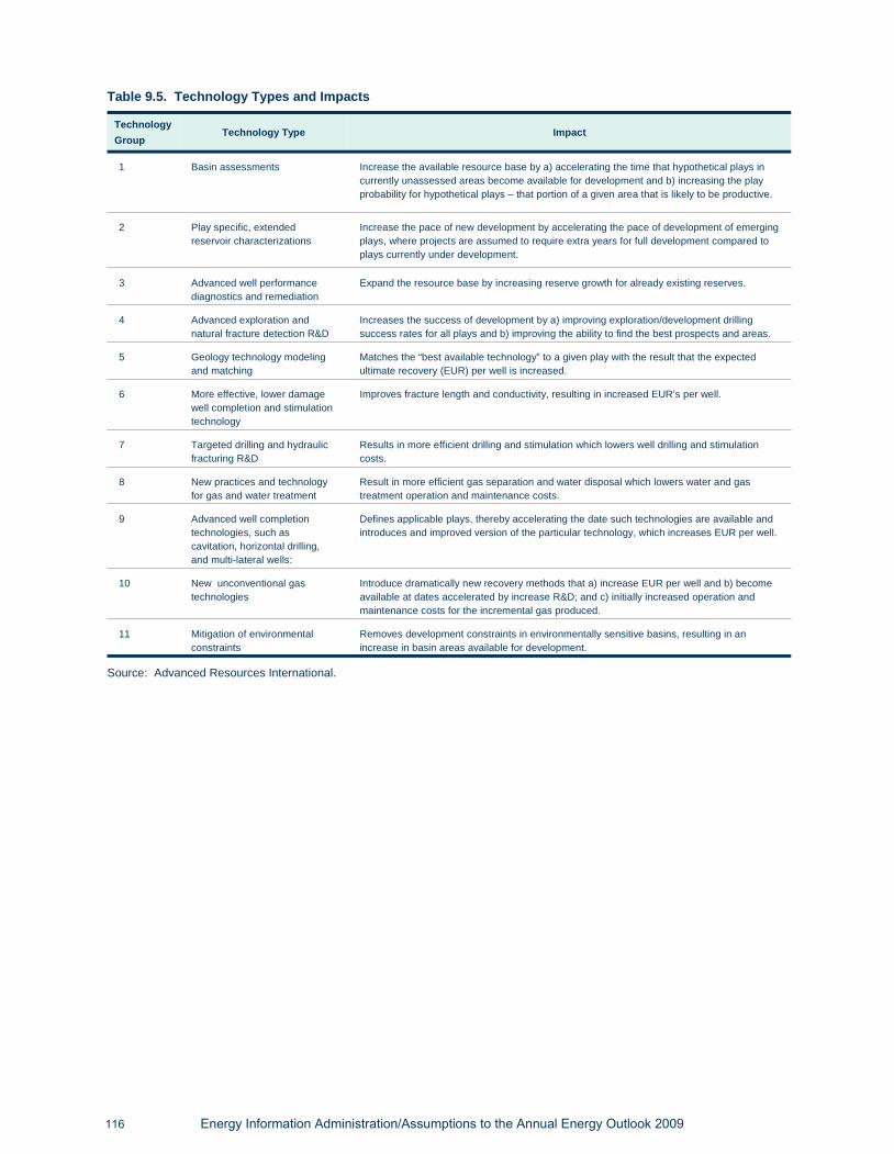
116 Energy Information Administration/Assumptions to the Annual Energy Outlook 2009
TechnologyGroup
Technology Type Impact
1 Basin assessments Increase the available resource base by a) accelerating the time that hypothetical plays incurrently unassessed areas become available for development and b) increasing the playprobability for hypothetical plays – that portion of a given area that is likely to be productive.
2 Play specific, extendedreservoir characterizations
Increase the pace of new development by accelerating the pace of development of emergingplays, where projects are assumed to require extra years for full development compared toplays currently under development.
3 Advanced well performancediagnostics and remediation
Expand the resource base by increasing reserve growth for already existing reserves.
4 Advanced exploration andnatural fracture detection R&D
Increases the success of development by a) improving exploration/development drillingsuccess rates for all plays and b) improving the ability to find the best prospects and areas.
5 Geology technology modelingand matching
Matches the “best available technology” to a given play with the result that the expectedultimate recovery (EUR) per well is increased.
6 More effective, lower damagewell completion and stimulationtechnology
Improves fracture length and conductivity, resulting in increased EUR’s per well.
7 Targeted drilling and hydraulicfracturing R&D
Results in more efficient drilling and stimulation which lowers well drilling and stimulationcosts.
8 New practices and technologyfor gas and water treatment
Result in more efficient gas separation and water disposal which lowers water and gastreatment operation and maintenance costs.
9 Advanced well completiontechnologies, such ascavitation, horizontal drilling,and multi-lateral wells:
Defines applicable plays, thereby accelerating the date such technologies are available andintroduces and improved version of the particular technology, which increases EUR per well.
10 New unconventional gastechnologies
Introduce dramatically new recovery methods that a) increase EUR per well and b) becomeavailable at dates accelerated by increase R&D; and c) initially increased operation andmaintenance costs for the incremental gas produced.
11 Mitigation of environmentalconstraints
Removes development constraints in environmentally sensitive basins, resulting in anincrease in basin areas available for development.
Table 9.5. Technology Types and Impacts
Source: Advanced Resources International.

Energy Information Administration/Assumptions to the Annual Energy Outlook 2009 117
Technology Case
Technology Group Item Type of Deposit Slow Reference Rapid
1 Year Hypothetical Plays Become Available All Types-Non DOEAll Types-DOE
NANA
NA2016
NA2009
2 Decrease in Extended Portion of DevelopmentSchedule for Emerging Plays (per year)
Coalbed Methane and Tight Sands - Non DOEGas Shales-Non DOEAll Types - DOE
0.83%1.25%1.25%
1.67%2.50%2.50%
2.50%3.75%3.75%
3 Expansion of Existing Reserves (per year -declining 0.1% per year; eg., 3.0, 2.0...)
Tight Sands
Coalbed Methane & Gas Shales
1.0%
2.0%
2.0%
4.0%
3.0%
6.0%
4 Increase in Percentage of Wells Drilled Successfully (per year)
All Types 0.1% 0.2% 0.3%
Year that Best 30 Percent of Basin is Fully Identified
All Types 2100 2044 2031
5 Increase in EUR per Well (per year) All Types 0.13% 0.25% 0.38%
6 Increase in EUR per Well (per year) All Types 0.13% 0.25% 0.38%
7 Decrease in Drilling and Stimulation Costs perWell (per year)
All Types NA NA NA
8 Decrease in Water and Gas Treatment O&MCosts per Well (per year)
All Types NA NA NA
9 Year Advanced Well CompletionTechnologies Become Available
Coalbed Methane
Tight Sands &GasShales
NA
NA
NA
2016
NA
2009
Increase in EUR per well (total increase) Coalbed Methane NA NA NA
Tight Sands NA 10% 15%
Gas Shales NA 20% 30%
10 Year Advanced Recovery Technologies Become Available
Coalbed Methane &Tight SandsGas Shales
NA
NA
NA
NA
2023
NA
Increase in EUR per well (total increase) Coalbed Methane NA NA 45%
Tight Sands NA NA 15%
Gas Shales NA NA NA
Increase in Costs ($1996/Mcf) for Incremental CBM production
Coalbed MethaneTight Sands
NANA
NANA
1.750.75
GasShales NA NA NA
11 Proportion of Areas Current Restricted that become Available for Development (per year)
All Types - Non DOEAll Types - DOE
0.5%0.25%
1.0%0.5%
1.5%0.75%
Table 9.6. Assumed Rates of Technological Progress for Unconventional Gas Recovery
EUR = Estimated Ultimate Recovery.O&M = Operation & Maintenance.CBM = Coalbed Methane.NA = Not applicable.DOE = Those plays in the Rocky Mountain basins assessed as part of Department of Energy sponsored basin studies.Source: Reference Technology Case, Advanced Resources, International; Slow and Rapid Technology Cases, Energy InformationAdministration, Office of Integrated Analysis and Forecasting.

Arctic National Wildlife Refuge (ANWR) CaseThe Arctic National Wildlife Refuge (ANWR) case assumes that Congressional legislation opening theFederal 1002 Area to Federal oil and gas leasing would be enacted in 2009.
The ANWR case is solely focused on the potential for ANWR to produce crude oil. The ANWR caseassumes that any gas found within ANWR would be re-injected into ANWR oil reservoirs to maintainreservoir pressure and that any Alaskan gas pipeline built during the projection period would rely on thenatural gas reserves and resources found within the State lands located in the Central North Slope.
The ANWR case assumes that the opening of the Federal 1002 Area would also open the Native lands andState offshore region to oil exploration. The Federal, State, and Native lands are referred to collectively asthe ANWR Coastal Plain. The ANWR case assumes that the size of the oil fields discovered within thecoastal plain is based on the mean U.S. Geological Survey (USGS) estimate of 10.4 billion barrels oftechnically recoverable crude oil8 that the USGS9 estimated for the Federal, State, and Native lands in oradjacent to ANWR.
The ANWR case assumes first production from the ANWR area would occur 10 years after the 2009enactment of legislation opening ANWR to oil and gas leasing. So first ANWR oil production would occur in2019, based on the following timeline:
• 2 to 3 years to obtain U.S. Bureau of Land Management (BLM) leases.
• 2 to 3 years to drill a single exploratory well, due to the limited winter drilling season.
• 1 to 2 years to develop a production development plan and obtain BLM approval for that plan.
• 3 to 4 years to construct the necessary infrastructure and to drill and complete development wells.
The 10-year timeline for developing ANWR petroleum resources assumes that there are no protracted legalbattles regarding the leasing and development of ANWR oil resources.
The ANWR case assumes that much of the oil resources in ANWR, like the other oil resources on Alaska’sNorth Slope, could be profitably developed given the current levels of technology and at current andprojected oil prices. This analysis also assumes that new fields in ANWR will begin development 2 yearsafter a prior ANWR field begins oil production.
The ANWR case uses the USGS mean oil resource estimate of potential field sizes in the coastal plain area.Because the larger fields are generally easier to find and cheaper to develop, the ANWR case assumes thatthe largest oil fields are developed first. Based on the 2-year time lag assumption between the developmentof successive oil fields and the USGS field size distribution, the ANWR case assumes the following oil fielddevelopment schedule:
118 Energy Information Administration/Assumptions to the Annual Energy Outlook 2009
Year In Which Field Begins Production ANWR Case Field Size(million barrels)
2018 1,370
2020 700
2022 700
2024 360
2026 360
2028 360
2030 360
Total 4,210
Source: Energy Information Administration, Office of Integrated Analysis and Forecasting.

Potential production from ANWR fields is based on the size of the field discovered and the productionprofiles of other fields of the same size in Alaska with similar geological characteristics. In general, fields areassumed to take 3 to 4 years to reach peak production, maintain peak production for 3 to 4 years, and thendecline until they are no longer profitable and are closed.
Energy Information Administration/Assumptions to the Annual Energy Outlook 2009 119

[1] Technically recoverable resources are resources in accumulations producible using current recoverytechnology but without reference to economic profitability.
[2] Proved reserves are the estimated quantities that analysis of geological and engineering datademonstrate with reasonable certainty to be recoverable in future years from known reservoirs underexisting economic and operating conditions.
[3] Inferred reserves are that part of expected ultimate recovery from known fields in excess ofcumulative production plus current reserves.
[4] Undiscovered resources are located outside oil and gas fields in which the presence of resources hasbeen confirmed by exploratory drilling; they include resources from undiscovered pools within confirmedfields when they occur as unrelated accumulations controlled by distinctly separate structural features orstratigraphic conditions.
[5] Donald L. Gautier and others, U.S. Department of Interior, U.S. Geological Survey, 1995 NationalAssessment of the United States Oil and Gas Resources, (Washington, D.C., 1995); U.S. Department ofInterior, Minerals Management Service, Report to Congress: Comprehensive Inventory of U.S. OCS Oiland Natural Gas Resources, (February 2006); and 2003 estimates of conventionally recoverablehydrocarbon resources of the Gulf of Mexico and Atlantic Outer Continental Shelf as of January 1, 2003.
[6] The amounts added (in billion barrels) among the various OGSM regions are as follows: Northeast0.4, Gulf Coast 5.0, Midcontinent 3.8, Southwest 4.1, Rocky Mountain 1.5, and West Coast 1.3.
[7] Source: Noyes Data Corporation, Oil Shale Technical Data Handbook, edited by Perry Nowacki, ParkRidge, New Jersey, 1981, pages 89-97. The Paraho Oil Shale Project design had a maximum productionrate of 100,000 syncrude barrels per day, which is used in the OSSS as the standard oil shale facilitysize.
[8] Technically recoverable resources are resources that can be produced using current technology.
[9] U.S. Department of Interior, U.S. Geological Survey, The Oil and Gas Resource Potential of the ArcticNational Wildlife Refuge 1002 Area, Alaska, Open File Report 98-34, 1999; U.S. Geological Survey,USGS Fact Sheet FS-028-01, April 2001; and, Oil and Gas Resources of the Arctic Alaska PetroleumProvince, by David W. Houseknecht and Kenneth J. Bird, U.S. Geological Survey Professional Paper1732–A, 2005.
120 Energy Information Administration/Assumptions to the Annual Energy Outlook 2009
Notes and Sources

Notes and Sources for Table 9.2
Note: Resources in areas where drilling is officially prohibited are not included in this table. Also, theAssociated-Dissolved Gas and the Alaska values are not explicitly utilized in the OGSM, but are includedhere to complete the table. The Alaska value does not include stranded Arctic gas.
Source: Onshore, State Offshore, and Alaska - U.S. Geological Survey (USGS) with adjustments toUnconventional Gas Recovery resources by Advanced Resources, International; Federal (OuterContinental Shelf) Offshore - Minerals Management Service (MMS); Proved Reserves -- EIA, Office ofOil and Gas. Table values reflect removal of intervening reserve additions between the date of the latestavailable assessment and January 1, 2007.
Energy Information Administration/Assumptions to the Annual Energy Outlook 2009 121
Notes and Sources


Natural Gas Transmission and DistributionModuleThe NEMS Natural Gas Transmission and Distribution Module (NGTDM) derives domestic natural gasproduction, wellhead and border prices, end-use prices, and flows of natural gas through the regionalinterstate network, for both a peak (December through March) and off peak period during each projectionyear. These are derived by solving for the market equilibrium across the three main components of thenatural gas market: the supply component, the demand component, and the transmission and distributionnetwork that links them. Natural gas flow patterns are a function of the pattern in the previous year, coupledwith the relative prices of the supply options available to bring gas to market centers within each of theNGTDM regions (Figure 8). The major assumptions used within the NGTDM are grouped into five generalcategories. They relate to (1) structural components of the model, (2) capacity expansion and pricing oftransmission and distribution services, (3) Arctic pipelines, and (4) imports and exports. A complete listing ofNGTDM assumptions and in-depth methodology descriptions are presented in Model Documentation:Natural Gas Transmission and Distribution Model of the National Energy Modeling System, ModelDocumentation 2008, DOE/EIA-M062(2008) (Washington, DC, 2008).
Energy Information Administration/Assumptions to the Annual Energy Outlook 2009 123
Figure 8. Natural Gas Transmission and Distribution Model Regions
Source: Energy Information Administration, Office of Integrated Analysis and Forecasting
Report #:DOE/EIA-0554(2009)
Release date: March 2009
Next release date: March 2010

Key Assumptions
Structural Components
The primary and secondary region-to-region flows represented in the model are shown in Figure 8. Primaryflows are determined, along with nonassociated gas production levels, as the model equilibrates supply anddemand. Associated-dissolved gas production is determined in the Oil and Gas Supply Module (OGSM).Secondary flows are established before the equilibration process and are generally set exogenously.Liquefied natural gas (LNG) imports are also not directly part of the equilibration process, but are set at thebeginning of each NEMS iteration in response to the price from the previous iteration. Flows and productionlevels are determined for each season, linked by seasonal storage. When required, annual quantities (e.g.,consumption levels) are split into peak and offpeak values based on historical averages. When multipleregions are contained in a Census Division, regional end-use consumption levels are approximated usinghistorical average shares. Pipeline and storage capacity are added as warranted by the relative volumesand prices. Regional pipeline fuel and lease and plant fuel consumption are established by applying anhistorically based factor to the flow of gas through a region and the production in a region, respectively.Prices within the network, including at the borders and the wellhead, are largely determined during theequilibration process. Delivered prices for each sector are set by adding an endogenously estimatedmarkup (generally a distributor tariff) to the regional representative citygate price. Supply curves and electricgenerator gas consumption are provided by other NEMS modules for subregions of the NGTDM regions,reflective of how their internal regions overlap with the NGTDM regions.
Capacity Expansion and Pricing of Transmission and Distribution Services
For the first 2 projection years, announced pipeline and storage capacity expansions (that are deemedhighly likely to occur) are used to establish limits on flows and seasonal storage in the model. Subsequently,pipeline and storage capacity is added when increases in consumption, coupled with an anticipated priceincrease, warrant such additions (i.e., flow is allowed to exceed current capacity if the demand still existsgiven an assumed increased tariff). Once it is determined that an expansion will occur, the associatedcapital costs are applied in the revenue requirement calculations in future years. Capital costs are assumedbased on average costs of recent comparable expansions for compressors, looping, and new pipeline.
It is assumed that pipeline and local distribution companies build and subscribe to a portfolio of interstatepipeline and storage capacity to serve a region-specific colder-than-normal winter demand level, currentlyset at 30 percent above the daily average. Maximum pipeline capacity utilization in the peak period is set at99 percent. In the off-peak period, the maximum is assumed to vary between 75 and 99 percent of thedesign capacity. The overall level and profile of consumption, as well as the availability and price of supplies,generally cause realized pipeline utilization levels to be lower than the maximum.
Pricing of Services
While transportation tariffs for interstate pipeline services are initially based on a regulated cost-of-servicecalculation, an adjustment to the tariffs is applied which is dependent on the realized utilization rate, to reflecta market-based differential. Transportation rates for interstate pipeline services (both between NGTDMregions and within a region) are calculated assuming that the costs of new pipeline capacity will be rolled intothe existing rate base.
Delivered prices by sector and season are derived by adding a markup to the average regional market priceof natural gas in both peak and off-peak periods. (Prices are reported on an annual basis and representquantity-weighted averages of the two seasons.) These markups include the cost of service provided byintraregional interstate pipelines, intrastate pipelines, and local distributors. The intrastate tariffs areaccounted for endogenously through historical model benchmarking. Distributor tariffs represent thedifference between the regional delivered and citygate price, independent of whether or not a customer classtypically purchases gas through a local distributor.
124 Energy Information Administration/Assumptions to the Annual Energy Outlook 2009

The distribution tariffs are projected using econometrically estimated equations, primarily in response tochanges in consumption levels. An assumed differential is used to divide the industrial price into one fornoncore customers (refineries and industrial boiler users) and one for core customers who have lessalternative fuel options.
The vehicle natural gas (VNG) sector is divided into fleet and non-fleet vehicles. In general, the distributortariffs for natural gas to vehicles are set to EIA’s Natural Gas Annual historical end-use prices minus citygateprices plus Federal and State VNG taxes (held constant in nominal dollars) plus an assumed dispensingcost. Dispensing costs are assumed to be $3.93 and $2.29 (2007 dollars per mcf) for non-fleet and fleetvehicles, respectively.
Pipelines from Arctic Areas into AlbertaThe outlook for natural gas production from the North Slope of Alaska is affected strongly by the uniquecircumstances regarding its transport to market. Unlike virtually all other identified deposits of natural gas inthe United States, North Slope gas lacks a means of economic transport to major commercial markets. Thelack of viable marketing potential at present has led to the use of Prudhoe Bay gas to maximize crude oilrecovery in that field. Recent high natural gas prices seemingly raised the potential economic viability ofsuch a project, although expected costs have increased as well. The primary assumptions associated withestimating the cost of North Slope Alaskan gas in Alberta, as well as for MacKenzie Delta gas into Alberta,are shown in Table 10.1. A calculation is performed to estimate a regulated, levelized, tariff for each pipeline.Additional items are added to account for the wellhead price, treatment costs, pipeline fuel costs, and a riskpremium to reflect the potential impact on the market price once the pipeline comes on line.
To assess the market value of Alaskan and Mackenzie Valley gas against the lower-48 market, a pricedifferential of $0.70 (2007 dollars per Mcf) is assumed between the price in Alberta and the average lower 48price. The resulting cost of Alaska gas, relative to the lower 48 wellhead price, is approximately $5.65 (2007dollars per Mcf), with some variation across the projection due to changes in gross domestic product.Construction of an Alaska-to-Alberta pipeline is projected to commence if the assumed total costs for Alaska gasin the lower 48 States exceeds the average lower 48 gas price in each of the previous 2 years, on average overthe previous 5 years (with greater weight applied to more recent years), and as expected to average over the next3 years. An adjustment is made if prices were declining over the previous 5 years. Once the assumed 4-yearconstruction period is complete, expansion can occur if the price exceeds the initial trigger price by $6.44 (2007dollars per Mcf). Supplies to fill an expanded pipeline are assumed to require new gas wells. When the Alaska toAlberta pipeline is built in the model, additional pipeline capacity is added to bring the gas across the border intothe United States. For accounting purposes, the model assumes that all of the Alaska gas will be consumed inthe United States and that sufficient economical supplies are available at the North Slope to fill the pipeline overthe depreciation period.
Natural gas production from the MacKenzie Delta is assumed to be sufficient to fill a pipeline over theprojection period should one be built connecting the area to markets in the south. The basic methodologyused to represent the decision to build a MacKenzie pipeline is similar to the process used for anAlaska-to-lower 48 pipeline, using the primary assumed parameters listed in Table 10.1. One exception isthat wellhead costs are assumed to change across the projection period with estimated changes to drillingcosts for the lower 48 States.
Supplemental Natural GasThe projection for supplemental gas supply is identified for three separate categories: pipeline quality syntheticnatural gas (SNG) from coal or coal-to-gas (CTG), SNG from liquids, and other supplemental supplies(propane-air, coke oven gas, refinery gas, biomass air, air injected for Btu stabilization, and manufactured gascommingled and distributed with natural gas). The third category, other supplemental supplies, are held at aconstant level of 10.3 billion cubic feet per year throughout the projection because this level is consistent withhistorical data and it is not believed to change significantly in the context of a reference case. SNG from liquidhydrocarbons in Hawaii is assumed to continue over the projection at the average historical level of 2.7 billioncubic feet per year. SNG production from coal at the currently operating Great Plains Coal Gasification Plant isalso assumed to continue through the projection period at an average historical level of 51.4 billion cubic feetper year. It is assumed that additional CTG facilities will be built if and when natural gas prices are highenough to make them economic. One CTG facility is assumed capable of processing 6,040 tons of
Energy Information Administration/Assumptions to the Annual Energy Outlook 2009 125

bituminous coal per day, with a production capacity of 0.1 Bcf per day of synthetic fuel and approximately100 megawatts of capacity for electricity cogeneration sold to the grid. A CTG facility of this size is assumedto cost over $1.05 billion in initial capital investment (2007 dollars). CTG facilities are assumed to be builtnear existing coal mines. All NGTDM regions are considered potential locations for CTG facilities except forNew England. Synthetic gas products from CTG facilities are assumed to be competitive when natural gasprices rise above the cost of CTG production (adjusted for credits from the sale of cogenerated electricity). Itis assumed that CTG facilities will not be built before 2012.
Natural Gas Imports and Exports
U.S. natural gas trade with Mexico is determined endogenously based on various assumptions about thenatural gas market in Mexico. U.S. natural gas exports from the United States to Canada are setexogenously in NEMS starting at 534 billion cubic feet per year in 2008 and increasing to 739 tcf by 2030.Canadian production and U.S. import flows from Canada are determined endogenously within the model.
Growth rates for consumption in Mexico are set exogenously based on projections from the InternationalEnergy Outlook 2008 and are provided in Table 10.2, along with initially assumed growth rates for productionin Mexico from the same source. Adjustments are made endogenously within the model to reflect a responseto price fluctuations within the market. Domestic production is assumed to be supplemented by LNG fromreceiving terminals constructed on both the east and west coasts of Mexico. The difference betweenproduction plus LNG imports and consumption in any year is assumed to be either imported from, orexported to, United States.
126 Energy Information Administration/Assumptions to the Annual Energy Outlook 2009
Alaska to Alberta MacKenzie Delta to Alberta
Initial flow into Alberta 3.9 Bcf per day 1.1 Bcf per day
Expansion potential 22 percent 58 percent
Initial capitalization 27.6 billion (2007 dollars) $10.2 billion (2007 dollars)
Cost of Debt (premium over BAA bondrate) 0.0 percent 0.0 percent
Cost of equity (premium over 10 yeartreasury yield note) 7.5 percent 7.5 percent
Debt fraction 60 percent 60 percent
Depreciation period 20 years 20 years
Minimum wellhead price (including $1.65 (2007 dollars per Mcf) $3.02 (2007 dollars per Mcf)
treatment and fuel costs)
Risk Premium $0.82 (2007 dollars per Mcf) $0.06 (2007 dollars per Mcf)
Additional cost for expansion $6.44 (2007 dollars per Mcf) $0.35 (2007 dollars per Mcf)
Construction period 4 years 4 years
Planning period 5 years 2 years
Earliest start year 2020 2014
Table 10.1. Primary Assumptions for Natural Gas Pipelines from Alaska and MacKenzie Delta into Alberta, Canada
Source: Energy Information Administration, Office of Integrated Analysis and Forecasting. Alaska pipeline cost data are based onNovember 2007 pipeline proposals submitted in compliance with the Alaska Gas line Inducement Act (A61A) requirements byConoco Phllips and Trans Canada Pipelines to the State of Alaska.
National Energy Board of Canada, “Mackenzie Gas Project – Hearing Order GH-1-2004, Supplemental Information – ProjectUpdate 2007,” dated May 15, 2007;
National Energy Board of Canada, “Mackenzie Gas Project – Project Cost Estimate and Schedule Update,” dated March 12, 2007;Canada Revenue Agency, “T2 Corporation Income Tax Guide 2006,” T4012(E) Rev. 07.Indian and Northern Affairs Canada, “Oil and Gas in Canada’s North,” website addresshttp://www.ainc-inac.gc.ca/ps/ecd/env/nor_e.html.National Energy Board of Canada, “Application for Approval of the Development Plan for Taglu Field - Project Description,”submitted by Imperial Oil Resources Ltd., TDPA-P1, August 2004;National Energy Board of Canada, “Application for Approval of the Development Plan for Niglintgak Field - Project Description,”submitted by Shell Canada Ltd., NDPA-P1, August 2004; andNational Energy Board of Canada, “Application for Approval of the Development Plan for Parsons Lake Field - ProjectDescription,” submitted by ConocoPhillips Canada (North) Ltd., PLDPA-P1, August 2004.

Canadian consumption and production in Eastern Canada are set exogenously in the model and are shownin Table 10.3. Production in the Western Canadian Sedimentary Basin (WCSB) is calculated endogenouslyto the model using annual supply curves based on beginning-of-year proved reserves and an estimatedproduction-to-reserve ratio. Reserve additions are set equal to the product of successful natural gas wellsand a finding rate (both based on an econometric estimation). The initial coalbed methane, shale gas, andconventional WCSB economically recoverable resource base estimates assumed in the model for thebeginning of 2004 are 70 trillion cubic feet, 30 trillion cubic feet (starting in 2010), and 92 trillion cubic feet,respectively.1 Potential production from tight formations was approximated by increasing the conventionalresource level by 1.5 percent annually. Production from coalbed and shale sources is established based onan assumed production path which varies in response to the level of remaining resources and the solutionprice in the previous projection year. To approximate the impact of the average increase in the Albertaroyalty rate, starting in 2009 the price drivers (i.e., the price realize by producers) on western Canada supplyin the model were assumed to be 5 percent less than they would have been otherwise.
Annual U.S. exports of liquefied natural gas (LNG) to Japan are assumed to decrease from 2007 levels of 44billion cubic feet per year through March of 2011, when the export license expires, and cease thereafter.LNG imports to the United States are determined endogenously within the model.
For the most part, LNG imports are set endogenously in the model based on Atlantic/Pacific andpeak/off-peak supply curves derived from model results generated by EIA’s International Natural Gas Model(INGM). Prices from the previous model iteration are used to establish the total level of North Americanimports in the peak or off-peak and in the Atlantic or Pacific. First assumed LNG imports which areconsumed in Mexico
2 are subtracted (presuming the volumes are sufficient) and the remaining levels are
allocated to the model regions based on last year’s import levels, the available regasification capacity, andthe relative prices. Regasification capacity is limited to facilities currently in existence and those alreadyunder construction and is fully sufficient to accommodate import levels projected by the model.
Energy Information Administration/Assumptions to the Annual Energy Outlook 2009 127
Consumption Production
2008 - 2010 1.0 0.1
2011- 2015 3.7 0.1
2016 - 2020 3.9 2.7
2021 - 2025 3.2 2.2
2026 - 2030 3.3 3.2
Table 10.2. Assumed Annual Growth Rates for Mexico (percent)
Source: EIA, International Energy Outlook 2008, DOE/EIA-0484(2008) and Energy Information Administration, Office ofIntegrated Analysis and Forecasting.
Year Consumption ProductionEastern Canada
2005 3,400 151
2010 3,700 240
2015 4,000 530
2020 4,300 670
2025 4,600 820
2030 5,000 710
Table 10.3. Exogenously Specified Canadian Production and Consumption (billion cubic feet per year)
Source: Consumption - EIA, International Energy Outlook 2008, DOE/EIA-0484(2008); Production - Energy InformatiionAdministration, Office of Integrated Analysis and Forecasting.

Legislation and Regulations
The methodology for setting reservation fees for transportation services is initially based on a regulated ratecalculation, but is ultimately consistent with FERC’s alternative ratemaking and capacity release position inthat it allows some flexibility in the rates pipelines ultimately charge. The methodology is market-based inthat rates for transportation services will respond positively to increased demand for services while rates willdecline (reflecting discounts to retain customers) should the demand for services decline.
A number of legislative actions have been taken to provide a more favorable environment for the introductionof new liquefied natural gas (LNG) regasification facilities in the United States. In December 2002 under theHackberry Decision, FERC terminated open access requirements for new onshore LNG terminals, placingthem on an equal footing with offshore terminals regulated under provisions of the Maritime Security Act of2002. The Maritime Security Act, signed into law in November 2002, also amended the Deepwater Port Actof 1974 to include offshore natural gas facilities, transferring jurisdiction for these facilities from the FERC tothe Maritime Administration and the U.S. Coast Guard. The result should be to streamline the permittingprocess and relax regulator requirements. More recently an EPACT2005 provision clarified the role of theFERC as the final decision making body on issues concerning onshore LNG facilities. While none of theselegislative/regulatory actions is explicitly represented in the modeling framework, these provisions areindirectly reflected in selected model parameters.
Section 116 of the Military Construction Appropriations and Emergency Hurricane SupplementalAppropriations Act, 2004 (H.R.4837) gives the Secretary of Energy the authority to issue Federal loanguarantees for an Alaska natural gas transportation project, including the Canadian portion, that would carrynatural gas from northern Alaska, through the Canadian border south of 68 degrees north latitude, intoCanada, and to the lower 48 States. This authority would expire 2 years after the final certificate of publicconvenience and necessity is issued. In aggregate the loan guarantee would not exceed: (1) 80 percent oftotal capital costs (including interest during construction); (2) $18 billion dollars (indexed for inflation at thetime of enactment); or (3) a term of 30 years. The Act also promotes streamlined permitting andenvironmental review, an expedited court review process, and protection of rights-of-way for the pipeline.The assumed costs of borrowing money for the pipeline was reduced to reflect the decreased risk as a resultof the loan guarantee.
Section 706 of the American Jobs Creation Act of 2004 (H.R.4520) provided a 7-year cost-of-investmentrecovery period for the Alaska natural gas pipeline, as opposed to the previously allowed 15-year recoveryperiod, for tax purposes. The provision is effective for property placed in service after 2013 (or treated assuch) and is assumed to have minimal impact on the decision to build the pipeline.
Section 707 of the American Jobs Creation Act extended the 15-percent tax credit previously applied tocosts related to enhanced oil recovery to construction costs for a gas treatment plant that supplies naturalgas to a 2 trillion Btu per day pipeline, lies in Northern Alaska, and produces carbon dioxide for injection intohydrocarbon-bearing geological formations. A gas treatment plan on the North Slope that feeds gas into anAlaska pipeline to Canada is expected to satisfy this requirement. The provision is effective for costsincurred after 2004. The impact of this tax credit is assumed to be factored into the cost estimates filed by theparticipating companies.
In 2005, Section 1113 of the Safe, Accountable, Flexible, Efficient Transportation Equity Act: A Legacy forUsers (SAFETEA-LU) raised the federal motor fuels tax for compressed natural gas vehicles (CNG) from48.54 cents per Mcf to 18.3 cents per gasoline gallon equivalent (or about $1.46 per Mcf), all in nominaldollars. The same section also allows for a motor fuels excise tax credit of $0.50 per gasoline gallonequivalent to the seller through September 30, 2009. The tax rate assumed in the model was changedaccordingly and assumed constant in nominal terms throughout the projection.
Section 312 of the Energy Policy Act of 2005 authorizes the Federal Energy Regulatory Commission (FERC)to allow natural gas storage facilities to charge market-based rates if it was believed that they would not exertmarket power. Storage rates are allowed to vary in the model from regulation-based rates, depending onmarket conditions.
128 Energy Information Administration/Assumptions to the Annual Energy Outlook 2009

Natural Gas Transmission and Distribution Alternative Cases
High and Low Liquefied Natural Gas Import CasesReference case assumptions regarding LNG imports to the U.S. reflect expectations of increasing globaldemand and non-competitive domestic natural gas prices relative to higher world LNG prices.
In the high LNG supply case, LNG imports to the U.S. are exogenously projected to increase over referencecase levels to determine the potential impact of additional LNG imports on the U.S. natural gas market. LNGimports are set by multiplying the reference case import levels by a factor which starts at 1.0, increaseslinearly between 2010 and 2030, and results in an LNG import level 5 times the reference case level by 2030.LNG imports in the high LNG case reach a level that approaches the projected regasification capacity in theUnited States in the reference case.
In the low LNG supply case, LNG imports to the U.S. are projected to remain constant at 2009 LNG importlevels from the reference case.
No Alaska North Slope Natural Gas Pipeline CaseThe construction of a natural gas pipeline from the North Slope of Alaska (ANS) to the lower 48 states hasbeen a matter of uncertainty for a number of years amidst increasing capital cost estimates and political andbusiness concerns existing between the state government and North Slope producers. In prior AEOprojections, the earliest start year for ANS pipeline transmission has generally been pushed back as theseissues delay construction of the pipeline. In the AEO2009 reference case, it is projected that the ANSpipeline will begin transporting natural to the lower 48 states beginning in 2020, the earliest assumed startyear.
In the No Alaska North Slope pipeline case, it is assumed that the ANS pipeline will not be built over theprojection period. This results in slightly higher imports and increased domestic production.
Energy Information Administration/Assumptions to the Annual Energy Outlook 2009 129

[1] For unconventional (i.e., coalbed) -- Average undiscovered resources under the National Energy Board'sSupply Push and Techno-vert scenarios in "Canada's Energy Future, Scenarios for Supply and Demand to2025," 2003. For conventional -- "Canada's Conventional Natural Gas Resources -- A Status Report," April2004. For shale gas a 5 percent recovery rate was assumed for a 600 trillion cubic feet estimate ofgas-in-place, which is lower than some estimates.
[2] LNG imports into Mexico, for consumption in the country, at the two existing facilities (in Altamira andBaja) are assumed to maintain at about 90 Bcf per year throughout the forecast. An additional facility isassumed to come on-line in 2011 in southwest Mexico and phase up to an import level of 90 Bcf per year aswell. These levels are based in part on Sener, “Prospectiva del Mercado de Gas Natural 2006-2015”.
130 Energy Information Administration/Assumptions to the Annual Energy Outlook 2009
Notes and Sources

Petroleum Market ModuleThe NEMS Petroleum Market Module (PMM) projects petroleum product prices and sources of supply formeeting petroleum product demand. The sources of supply include crude oil (both domestic and imported),petroleum product imports, unfinished oil imports, other refinery inputs (including alcohols, ethers, bioesters,corn, biomass, and coal), natural gas plant liquids production, and refinery processing gain. In addition, the PMMprojects capacity expansion and fuel consumption at domestic refineries.
The PMM contains a linear programming (LP) representation of U.S. refining activities in the five Petroleum AreaDefense Districts (PADDs) (Figure 9), linked to a simplified world refining industry representation used tomodel U.S. crude and product imports. The U.S. segment of the LP model is created by aggregating individualU.S. refineries within a PADD into two types of representative refineries, and linking all five PADD’s and worldrefining regions via crude and product transit links. This representation provides the marginal costs of productionfor a number of conventional and new petroleum products. In order to interact with other NEMS moduleswith different regional representations, certain PMM inputs and outputs are converted from PADD regionsto other regional structures and vice versa. The linear programming results are used to determine end-useproduct prices for each Census Division (shown in Figure 5) using the assumptions and methods describedbelow.
Energy Information Administration/Assumptions to the Annual Energy Outlook 2009 131
AK
WA
NV
AZ
OR
CA
HI
V
MT
WY
ID
UTCO
IV
OK
IA
KS
MO
ILIN
KY
TN
WI
MI
OH
NE
SD
MNND
II
NM
TX
MS
ALAR
LAIII
NJCT
VT ME
RIMA
NHNY
PAI
Figure 9. Petroleum Administration for Defense Districts
Source:Energy Information Administration,Office of Integrated Analysis and Forecasting.
Report #:DOE/EIA-0554(2009)Release date: March 2009Next release date: March 2010

Key Assumptions
Product Types and SpecificationsThe PMM models refinery production of the products shown in Table 11.1.
The costs of producing different formulations of gasoline and diesel fuel that are required by State andFederal regulations are determined within the linear programming representation of refineries byincorporating the specifications and demands for these fuels. The PMM assumes that the specifications forthese fuels will remain the same as currently specified, with a few exceptions: the sulfur content, which will bephased down to reflect EPA regulations for all gasoline and diesel fuels; and, benzene content, which will bereduced in gasoline beginning in 2011.
Motor Gasoline Specifications and Market SharesThe PMM models the production and distribution of three different types of gasoline: conventional,oxygenated, and reformulated (Phase 2). The following specifications are included in the PMM todifferentiate between conventional and reformulated gasoline blends (Table 11.2): Reid vapor pressure (RVP),benzene content, aromatic content, sulfur content, olefins content, and the percent evaporated at 200 and 300degrees Fahrenheit (E200 and E300). The sulfur content specification for gasoline has been reduced annuallythrough 2007 to reflect recent regulations requiring the average annual sulfur content of all gasoline used in theUnited States to be phased-down to 30 parts per million (ppm) between 2004 and 2007.1 The sulfur specificationsassumed for each region and type of gasoline are provided in Table 11.3.
Conventional gasoline must comply with antidumping requirements aimed at preventing the quality ofconventional gasoline from eroding as the reformulated gasoline program is implemented. Conventionalgasoline must meet the Complex Model II compliance standards which cannot exceed average 1990 levels oftoxic and nitrogen oxide emissions.2
Oxygenated gasoline is assumed to have specifications identical to conventional gasoline, with theexception of a higher oxygen requirement, specifically 2.7 percent oxygen by weight. Some areas thatrequire oxygenated gasoline will also require reformulated gasoline. For the sake of simplicity, the areas ofoverlap are assumed to require gasoline meeting the reformulated specifications.
Cellulosic biomass feedstock supplies and costs are taken from the NEMS Renewable Fuels Model. Initialcapital costs for biomass cellulosic ethanol were obtained from a research project reviewing cost estimates frommultiple sources.3 Operating costs and credits for excess electricity generated at biomass ethanol plantswere obtained from a survey of recent literature4 and the USDA Agricultural Baseline Projections to 2015.5
132 Energy Information Administration/Assumptions to the Annual Energy Outlook 2009
Product Category Specific Products Motor Gasoline Conventional Unleaded, Oxygenated, Reformulated
Jet Fuel Kerosene-type
Distillates Kerosene, Heating Oil, Low-Sulfur-Diesel, Ultra-Low-Sulfur-Diesel
Residual Fuels Low Sulfur, High Sulfur
Liquefied Petroleum Gases Propane, Liquefied Petroleum Gases Mixed
Petrochemical Feedstocks Petrochemical Naptha, Petrochemical Gas Oil, Propylene, Aromatics
Others Lubricating Products and Waxes, Asphalt/Road Oil, Still GasPetroleum Coke, Special Naphthas, Aviation Gasoline
Table 11.1. Petroleum Product Categories
Source: Energy Information Administration, Office of Integrated Analysis and Forecasting.

Energy Information Administration/Assumptions to the Annual Energy Outlook 2009 133
PADD
ReidVapor
Pressure(Max PSI)
AromaticsVolumePercent
(Max)
BenzeneVolume Percent (Max)
2007SulfurPPM
(Max)
OlefinVolumePercent(Max)
Percent Evaporated
at200o
Percent Evaluated
at300o
Conventional
PADD I 9.6 26.0 1.1 30.0 11.6 47.1 82.0
PADD II 10.2 26.1 1.1 30.0 11.6 47.1 81.9
PADD III 9.9 26.1 1.1 30.0 11.6 47.1 81.9
PADD IV 10.8 26.1 1.1 30.0 11.6 47.1 81.9
PADD V 9.2 26.7 1.1 30.0 11.7 45.7 81.4
Reformulated PADD I 8.5 20.7 0.6 30.0 11.9 50.2 84.6
PADD II 9.5 18.5 0.8 30.0 7.1 50.8 85.2
PADD III 8.6 19.8 0.6 30.0 11.2 51.6 83.9
PADD IV 8.6 19.8 0.6 30.0 11.2 51.6 83.9
PADD V
Nonattainment 7.9 22.0 0.70 20.0 6.0 49.0 90.0
CARB (attainment) 7.9 22.0 0.70 20.0 6.0 49.0 90.0
Table 11.2. Year Round Gasoline Specifications by Petroleum Administration for Defense Districts (PADD)
Max = Maximum.
PADD = Petroleum Administration for Defense District.
PPM = Parts per Million by Weight.
PSI = Pounds per Square Inch.
Volume percent will change to 0.6 in 2011to meet the MSAT2 ruling.
Source: Energy Information Administration, Office of Integrated Analysis and Forecasting. Derived using U.S. EPA’sComplex Model, and updated with U.S. EPA's gasoline projection survey “Fuel Trends Report: Gasoline 1995-2005”, January2008, EPA420-R-08-002 (http://www.epa.gov/otaq/regs/fuels/rfg/properf/rfgperf.htm).(http://www.epa.gov/otaq/regs/fuels/rfg/properf/rfgperf.htm).
2004 2005 2006 2007 2008-2030
Conventional
PADD I 143.4 90.0 43.4 41.7 30
PADD II 111.6 60.0 32.2 32.2 30
PADD III 114.5 60.0 32.4 32.4 30
PADD IV 140.0 90.0 44.2 44.2 30
PADD V 122.8 70.0 33.7 33.7 30
ReformulatedPADD I-IV 30 30 30 30 30
PADD V 20 20 20 20 20
Table 11.3. Gasoline Sulfur Content Assumptions, by Region and Gasoline Type, Parts per Million (PPM)
Source: Energy Information Administration, Office of Integrated Analysis and Forecasting. Derived from Form EI-810“Monthly Refinery Report” and U.S. Environmental Protection Agency, “Tier 2” Motor Vehicle Emissions Standards andGasoline Sulfur Control requirements, February 2000, (Washington, DC).
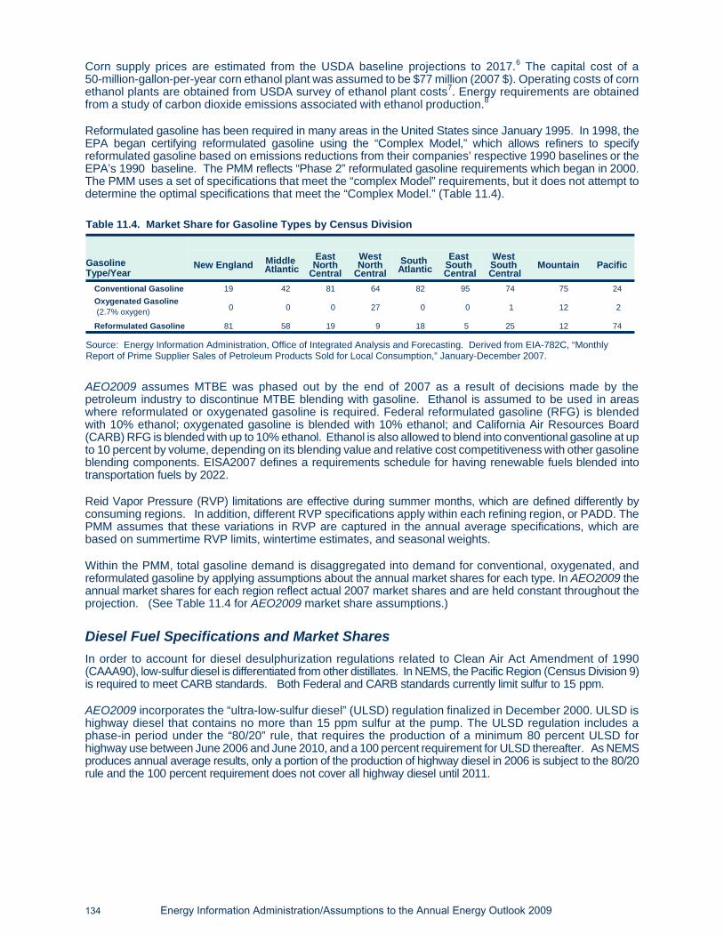
Corn supply prices are estimated from the USDA baseline projections to 2017.6 The capital cost of a50-million-gallon-per-year corn ethanol plant was assumed to be $77 million (2007 $). Operating costs of cornethanol plants are obtained from USDA survey of ethanol plant costs7. Energy requirements are obtainedfrom a study of carbon dioxide emissions associated with ethanol production.8
Reformulated gasoline has been required in many areas in the United States since January 1995. In 1998, theEPA began certifying reformulated gasoline using the “Complex Model,” which allows refiners to specifyreformulated gasoline based on emissions reductions from their companies’ respective 1990 baselines or theEPA’s 1990 baseline. The PMM reflects “Phase 2” reformulated gasoline requirements which began in 2000.The PMM uses a set of specifications that meet the “complex Model” requirements, but it does not attempt todetermine the optimal specifications that meet the “Complex Model.” (Table 11.4).
AEO2009 assumes MTBE was phased out by the end of 2007 as a result of decisions made by thepetroleum industry to discontinue MTBE blending with gasoline. Ethanol is assumed to be used in areaswhere reformulated or oxygenated gasoline is required. Federal reformulated gasoline (RFG) is blendedwith 10% ethanol; oxygenated gasoline is blended with 10% ethanol; and California Air Resources Board(CARB) RFG is blended with up to 10% ethanol. Ethanol is also allowed to blend into conventional gasoline at upto 10 percent by volume, depending on its blending value and relative cost competitiveness with other gasolineblending components. EISA2007 defines a requirements schedule for having renewable fuels blended intotransportation fuels by 2022.
Reid Vapor Pressure (RVP) limitations are effective during summer months, which are defined differently byconsuming regions. In addition, different RVP specifications apply within each refining region, or PADD. ThePMM assumes that these variations in RVP are captured in the annual average specifications, which arebased on summertime RVP limits, wintertime estimates, and seasonal weights.
Within the PMM, total gasoline demand is disaggregated into demand for conventional, oxygenated, andreformulated gasoline by applying assumptions about the annual market shares for each type. In AEO2009 theannual market shares for each region reflect actual 2007 market shares and are held constant throughout theprojection. (See Table 11.4 for AEO2009 market share assumptions.)
Diesel Fuel Specifications and Market SharesIn order to account for diesel desulphurization regulations related to Clean Air Act Amendment of 1990(CAAA90), low-sulfur diesel is differentiated from other distillates. In NEMS, the Pacific Region (Census Division 9)is required to meet CARB standards. Both Federal and CARB standards currently limit sulfur to 15 ppm.
AEO2009 incorporates the “ultra-low-sulfur diesel” (ULSD) regulation finalized in December 2000. ULSD ishighway diesel that contains no more than 15 ppm sulfur at the pump. The ULSD regulation includes aphase-in period under the “80/20” rule, that requires the production of a minimum 80 percent ULSD forhighway use between June 2006 and June 2010, and a 100 percent requirement for ULSD thereafter. As NEMSproduces annual average results, only a portion of the production of highway diesel in 2006 is subject to the 80/20rule and the 100 percent requirement does not cover all highway diesel until 2011.
134 Energy Information Administration/Assumptions to the Annual Energy Outlook 2009
GasolineType/Year
New England Middle Atlantic
East NorthCentral
West NorthCentral
SouthAtlantic
EastSouthCentral
WestSouthCentral
Mountain Pacific
Conventional Gasoline 19 42 81 64 82 95 74 75 24Oxygenated Gasoline (2.7% oxygen) 0 0 0 27 0 0 1 12 2
Reformulated Gasoline 81 58 19 9 18 5 25 12 74
Table 11.4. Market Share for Gasoline Types by Census Division
Source: Energy Information Administration, Office of Integrated Analysis and Forecasting. Derived from EIA-782C, “MonthlyReport of Prime Supplier Sales of Petroleum Products Sold for Local Consumption,” January-December 2007.
NEMS models ULSD as containing 7.5 ppm sulfur at the refinery gate in 2006, phasing down to 7ppm sulfur by2011. This lower sulfur limit at the refinery reflects the general consensus that refiners will need to producediesel with a sulfur content below 10 ppm to allow for contamination during the distribution process.
It is assumed that revamping (retrofitting) existing refinery units to produce ULSD will be undertaken byrefineries representing two-thirds of highway diesel production and that the remaining refineries will buildnew units. The capital cost of revamping is assumed to be 50 percent of the cost of adding a new unit.
The amount of ULSD downgraded to a lower value product because of sulfur contamination in thedistribution system is assumed to be 7.8 percent at the start of the program, declining to 2.2 percent at fullimplementation. The decline reflects the expectation that the distribution system will become more efficient athandling ULSD with experience.
A revenue loss is assumed to occur when a portion of ULSD that is put into the distribution system iscontaminated and must be sold as a lower value product. The amount of the revenue loss is estimatedoffline based on earlier NEMS results and is included in the AEO2009 ULSD price projections as adistribution cost. The revenue loss associated with the 7.8 percent downgrade assumption for 2009 is 0.7 centsper gallon. The revenue loss estimate declines to 0.2 cents per gallon after 2010 to reflect the assumeddecline to 2.2 percent.
The capital and operating costs associated with ULSD distribution are based on assumptions used by the EPAin the Regulatory Impact Analysis (RIA) of the rule.9 Capital costs of 0.7 cents per gallon are assumed foradditional storage tanks needed to handle ULSD during the transition period. These capital expenditures areassumed to be fully amortized by 2011. Additional operating costs for distribution of highway diesel of 0.2 centsper gallon are assumed over the entire projection period. Another 0.2 cent cost per gallon is assumed forlubricity additives. Lubricity additives are needed to compensate for the reduction of aromatics andhigh-molecular-weight hydrocarbons stripped away by the severe hydrotreating used in thedesulphurization process.
Demand for highway-grade diesel, both 500 ppm and ULSD combined, is assumed to be equivalent to the totaltransportation distillate demand. Historically, highway-grade diesel supplies have nearly matched totaltransportation distillate sales, although some highway-grade diesel has gone to nontransportation usessuch as construction and agriculture.
The energy content of ULSD is assumed to decline from that of 500 ppm diesel by 0.5 percent becauseundercutting and severe desulphurization will result in a lighter stream composition than that for 500 ppmdiesel.
AEO2009 incorporates the “nonroad, locomotive, and marine” (NRLM) diesel regulation finalized in May2004. The PMM model has been revised to reflect the nonroad rule and re-calibrated for market shares ofhighway, NRLM diesel, and other distillate (mostly heating oil, but excluding jet fuel and kerosene). TheNRLM diesel rule follows the highway diesel rule closely and represents an incremental tightening of theentire diesel pool. The demand for high sulfur distillate is expected to diminish over time, while the demand forULSD (both highway and NRLM) is expected to increase over time.
The final NRLM rule is implemented in multiple steps and requires sulfur content for all NRLM diesel fuelproduced by refiners to be reduced to 500 ppm starting mid-2007. It also establishes a new ultra-low-sulfur diesel(ULSD) limit of 15 ppm for nonroad diesel by mid-2010. For locomotive and marine diesel, the rule establishesan ULSD limit of 15 ppm in mid-2012.
End-Use Product Prices
End-use petroleum product prices are based on marginal costs of production plus production-related fixedcosts plus distribution costs and taxes. The marginal costs of production are determined within the LP andrepresent variable costs of production, including additional costs for meeting reformulated fuels provisions of theCAAA90. Environmental costs associated with controlling pollution at refineries are implicitly assumed in theannual update of the refinery investment costs for the processing units.
The costs of distributing and marketing petroleum products are represented by adding product-specificdistribution costs to the marginal refinery production costs (product wholesale prices). The distribution costs arederived from a set of base distribution markups (Table 11.5).
Energy Information Administration/Assumptions to the Annual Energy Outlook 2009 135

136 Energy Information Administration/Assumptions to the Annual Energy Outlook 2009
Sector/Product
Census Division
NewEngland
MiddleAtlantic
EastNorth
Central
West NorthCentral
SouthAtlantic
EastSouthCentral
West South
Central Mountain Pacific
Residential Sector
Distillate Fuel Oil 0.46 0.54 0.27 0.21 0.40 0.27 0.41 0.19 0.33
Kerosene 0.37 0.39 0.35 0.35 0.38 0.42 0.40 0.83 0.04
Liquefied Petroleum Gases 1.13 1.14 0.69 0.48 1.11 0.99 0.97 0.81 1.07
Commercial Sector
Distillate Fuel Oil 0.22 0.18 0.10 0.06 0.05 0.05 0.06 -0.04 0.08
Gasoline 0.16 0.18 0.14 0.12 0.12 0.14 0.14 0.14 0.17
Kerosene 0.36 0.35 0.35 0.34 0.37 0.40 0.33 0.81 0.40
Liquefied Petroleum Gases 0.52 0.66 0.57 0.57 0.63 0.60 0.63 0.69 0.61
Low-Sulfur Residual Fuel Oil 0.48 0.01 1.10 1.10 -0.03 1.20 0.00 0.75 1.33
Utility Sector
Distillate Fuel Oil 0.00 0.00 0.00 0.00 0.00 0.0 0.00 0.00 0.00
High-Sulfur Residual Fuel Oil1 0.17 -0.13 1.10 0.86 -0.13 -0.29 1.04 0.86 1.35
Low-Sulfur Residual Fuel Oil1 -0.11 -0.13 0.81 0.86 -0.13 -0.29 0.80 0.61 0.86
Transportation Sector
Distillate Fuel Oil 0.32 0.26 0.18 0.14 0.17 0.17 0.18 0.16 0.22
E852 0.12 0.16 0.11 0.09 0.11 0.11 0.11 0.11 0.12
Gasoline 0.15 0.21 0.14 0.12 0.14 0.14 0.14 0.14 0.15
High-Sulfur Residual Fuel Oil1 0.11 -0.07 0.22 0.30 0.14 0.22 0.21 0.43 -0.13
Jet Fuel 0.00 0.00 0.00 0.00 0.00 0.00 0.00 0.00 0.00
Liquefied Petroleum Gases 0.38 0.57 0.78 0.78 0.66 0.77 0.74 0.66 0.55
Industrial Sector
Asphalt and Road Oil 0.00 0.00 0.00 0.00 0.00 0.00 0.00 0.00 0.00
Distillate Fuel Oil 0.23 0.21 0.18 0.14 0.11 0.13 0.13 0.05 0.09
Gasoline 0.16 0.19 0.14 0.11 0.14 0.14 0.14 0.14 0.15
Kerosene 0.00 0.00 0.00 0.01 0.01 0.04 0.11 0.41 0.00
Liquefied Petroleum Gases 0.55 0.64 0.51 0.50 0.56 0.44 0.51 0.70 0.62
Low-Sulfur Residual Fuel Oil 0.45 -0.15 1.01 0.96 0.44 0.99 0.75 -0.18 0.13
Table 11.5. Petroleum Product End-Use Markups by Sector and Census Division(2007 dollars per gallon)
1Negative values indicate that average end-use sales prices were less than wholesale prices. This often occurs with residual fuelwhich is produced as a byproduct when crude oil is refined to make higher value products like gasoline and heating oil.274 percent ethanol and 26 percent gasoline.
Sources: Markups based on data from Energy Information Administration (EIA), Form EIA-782A, Refiners’/Gas Plant Operators’Monthly Petroleum Product Sales Report; EIA, Form EIA-782B, Resellers’/Retailers’ Monthly Petroleum Report Product SalesReport; EIA, Form FERC-423, Monthly Report of Cost and Quality of Fuels for Electric Plants; EIA, Form EIA-759 Monthly PowerPlant Report; EIA, State Energy Data Report 2006, Consumption (November 2008); EIA, State Energy Data 2006: Prices andExpenditures (November 2008).

State and Federal taxes are also added to transportation fuels to determine final end-use prices (Tables 11.6 and11.7). Recent tax trend analysis indicates that State taxes increase at the rate of inflation, therefore, State taxes areheld constant in real terms throughout the projection. This assumption is extended to local taxes which areassumed to average 2 cents per gallon.10 Federal taxes are assumed to remain at current levels in accordancewith the overall AEO2009 assumption of current laws and regulations. Federal taxes are deflated toconstant 2007$ as follows:
Federal Tax product, year = Current Federal Tax product / GDP Deflator year
Crude Oil Quality
In the PMM, the quality of crude oil is characterized by average gravity and sulfur levels. Both domestic andimported crude oil are divided into five categories as defined by the ranges of gravity and sulfur shown inTable 11.8.
Energy Information Administration/Assumptions to the Annual Energy Outlook 2009 137
Year/Product
Census Division
NewEngland
Middle Atlantic
East North
Central
West NorthCentral
South Atlantic
East SouthCentral
West SouthCentral
Mountain Pacific
Gasoline1 0.28 0.24 0.23 0.21 0.18 0.20 0.20 0.21 0.21
Diesel 0.24 0.28 0.22 0.21 0.21 0.18 0.19 0.23 0.21
Liquefied Petroleum Gases 0.13 0.13 0.18 0.20 0.19 0.18 0.14 0.15 0.06
E852 0.25 0.26 0.25 0.22 0.19 0.20 0.22 0.23 0.23
Jet Fuel 0.07 0.05 0.00 0.03 0.05 0.06 0.03 0.04 0.03
Table 11.6. State and Local Taxes on Petroleum Transportation Fuels by Census Division, as of July 2008 (2007 dollars per gallon)
1Tax also applies to gasoline consumed in the commercial and industrial sectors.2 74 percent ethanol and 26 percent gasoline.
Source: “Compilation of United States Fuel Taxes, Inspection, Fees and Environmental Taxes and Fees,” Defense EnergySupport Center, Editions 2008-10, July 3, 2008
Product Tax
Gasoline 0.18
Diesel 0.24
Jet Fuel 0.04
Liquefied Petroleum Gases3 0.183
M851 0.09
E852 0.20
Table 11.7 Federal Taxes, as of 2008 (Nominal dollars per gallon)
185 percent methanol and 15 percent gasoline.274 percent ethanol and 26 percent gasoline.32010 data-based on EPACT05: excise tax is 4.3 cents/gal after 9-30-2011 and 18.3 cents/gal prior to that. A credit of 50cents/gal is also applied between 10-1-06 and 9-30-09.
Sources: Omnibus Budget Reconciliation Act of 1993 (H.R. 2264); Tax Payer Relief Act of 1997 (PL 105-34), Clean Fuels Report(Washington, DC, April 1998) and Energy Policy Act of 2005 (PL 109-58). IRS Internal Revenue Bulletin 2006-43 available on theweb at http://www.irs.gov/pub/irs-irbs/irb06-43.pdf

A “composite” crude oil with the appropriate yields and qualities is developed for each category by averaging thecharacteristics of specific crude oil streams in the category. While the domestic and foreign categories are thesame, the composite crudes for each category may differ because different crude streams make up thecomposites. For domestic crude oil, estimates of total regional production are made first, then shared out to eachof the five categories based on historical data. For imported crude oil, a separate supply curve is provided foreach of the five categories. Each import supply curve is linked to a world oil supply market balance for that crudetype, such that the quantity of crude oil imported depends on the economic competition with use by the rest of theworld.
Capacity ExpansionPMM allows for capacity expansion of all processing unit types including distillation, vacuum distillation,hydrotreating, coking, fluid catalytic cracking, hydrocracking, and alkylation manufacturing. Capacityexpansion occurs by processing unit, starting from base year capacities established by PADD usinghistorical data.
Expansion occurs in NEMS when the value received from the additional product sales exceeds theinvestment and operating costs of the new unit. The investment costs assume a financing ratio of 60 percentequity and 40 percent debt, with a hurdle rate and an after-tax return on investment of about 9 percent.Capacity expansion plans are determined every 3 years. For example, the PMM looks ahead in 2008 anddetermines the optimal capacities given the estimated demands and prices expected in the 2011 projection year.The PMM then allows any of that capacity to be built in each of the projection years 2009, 2010, and 2011. At theend of 2011 the cycle begins anew, looking ahead to 2014. ACU capacity under construction that is expected tobegin operating during by 2010 is added to existing capacities in their respective start year. Capacityexpansion is also modeled for corn and cellulosic ethanol, coal-to-liquids, gas-to-liquids, andbiomass-to-liquids production.
Biofuels SupplyThe PMM provides supply functions on an annual basis through 2030 for ethanol produced from both corn andcellulosic biomass to produce transportation fuel. It also assumes that small amounts of vegetable oil andanimal fats are processed into biodiesel, a blend of methyl esters suitable for fueling diesel engines.
• Corn feedstock supplies and costs are provided exogenously to NEMS. Feedstock costs reflectcredits for co-products (livestock feed, corn oil, etc.). Feedstock supplies and costs reflect thecompetition between corn and its co-products and alternative crops, such as soybeans and theirco-products.
• Cellulosic (biomass) feedstock supply and costs are provided by the Renewable Fuels Module inNEMS. Cellulosic ethanol production and biomass-to-liquids (BTL) production compete for thisfeedstock.
• The Federal motor fuels excise tax credit for ethanol is 51 cents per gallon of ethanol (5.1 cents pergallon credit to gasohol at a 10-percent volumetric blending portion) is applied within the model. Thetax credit is held constant in nominal terms, decreasing with inflation throughout the projection in constantdollar terms. It is assumed that the credit expires after 2010.
138 Energy Information Administration/Assumptions to the Annual Energy Outlook 2009
Crude Oil Categories Sulfur(percent)
Gravity(degrees API)
Low Sulfur Light 0 - 0.5 25 - 60
Medium Sulfur Heavy 0.35 - 1.1 26 - 40
High Sulfur Light > 1.1 >32
High Sulfur Heavy > 1.1 24 - 33
High Sulfur Very Heavy > 0.9 < 23
Table 11.8. Crude Oil Specifications
Source: Energy Information Administration, Office of Integrated Analysis and Forecasting. Derived from EI-810, “MonthlyRefinery Report” data.

To model the new Renewable Fuels Standard in EISA2007, several assumptions were required. In addition tousing the text of the legislation it was also assumed that rules promulgated under the RFS in EPACT05would govern the administration of the EISA2007 RFS
• The penetration of cellulosic ethanol into the market is limited before 2012 to the projects(co-sponsored by DOE grants) currently scheduled to produce approximately 150 million gallons peryear.
• Biomass-to-Liquid (Fischer-Tropsch) diesel fuel production contributes 1.5 credits towards thecellulosic mandate.
• Imported cane ethanol counts toward the advanced renewables mandate. In addition, a limited supplyof cellulosic ethanol would be available for import and would count toward the cellulosic mandate.
• The cellulosic biofuel waiver, when activated, reduces the cellulosic, advanced, and total requirement bythat amount in all future years. In years beyond 2022, the last year specified in the EISA, the RFSmandate levels are held constant.
• It is assumed that biodiesel and BTL diesel may be consumed in diesel engines without significantinfrastructure modification (either vehicles or delivery infrastructure).
• Ethanol is assumed to be consumed as either E10 or E85, with no intermediate blends. The cost ofplacing E85 pumps at the most economic stations is spread over all transportation fuels. Using thisassumption, the E10 blending market is assumed to be saturated and the E85 market consumesadditional ethanol after 2014.
• To accommodate the ethanol requirements in particular, transportation modes are expanded orupgraded for both E10 and E85, and it is assumed that most ethanol originates from the Midwest, withtransportation costs ranging from a low of 1.7 cents per gallon for expanded distribution in theMidwest, to as high as 2.6 cents per gallon for the Southeast and West Coast.
• For E85 dispensing stations, it is assumed the average cost of a retrofit and new station is about$45,000 per station, which translates into an incremental cost per gallon ranging from 26 cents in 2013to 4.4 cents by 2020, depending on the average sales per dispenser.
• The total projected incremental infrastructure cost (transportation, distribution, dispensing) for E85 variesfrom 27 cents per gallon in 2013 to 6 cents per gallon in 2020
Interregional transportation is assumed to be by rail, ship, barge, and truck, and the associated costs areincluded in PMM. A subsidy is offered by the Department of Agriculture’s Commodity Credit Corporation forthe production of biodiesel. In addition, the American Jobs Creation Act of 2004 provides an additional taxcredit of $1 per gallon of soybean oil for biodiesel and 50 cents per gallon for yellow grease biodiesel until2006, and EPACT05 extended the credit again to 2008. The Emergency Stabilization Act of 2008 extended itagain to 2009 and increased the yellow grease credit to $1 per gallon.
Gas-To-Liquids, Coal-To-Liquids, and Gasification Technologies
Gas-to-liquids (GTL) facilities convert natural gas into distillates, and are assumed to be built if the prices for lowersulfur distillates reach a high enough level to make it economic. In the PMM, gas-to-liquids facilities are assumed tobe built only on the North Slope of Alaska, where the distillate product is transported on the Trans-Alaskan PipelineSystem (TAPS) to Valdez and shipped to markets in the lower 48 States. The earliest start date for a GTLfacility is set at 2017. Also, the source of feedstock gas to any GTL facility in Alaska is assumed to be fromundiscovered, non-associated resources which will be more costly than the current, largely associated provedreserves on the North Slope, which are assumed to be dedicated to the pipeline. The GTL facilities are builtincrementally, with output volumes of 34,000 barrels per day, at an capital cost of $52,023 per barrel of dailycapacity (2007 dollars). Variable operating costs are assumed to be $4.67 per barrel (2007 dollars). Thetransportation cost to ship the GTL product from the North Slope to Valdez along the TAPS is assumed to be
Energy Information Administration/Assumptions to the Annual Energy Outlook 2009 139

the price set to move oil (i.e. the TAPS revenue recovery rate). This rate is a function of allowable costs, profit,and flow, and can change over the projection.
It is also assumed that coal-to-liquids (CTL) facilities will be built when low-sulfur distillate prices are high enoughto make them economic. One CTL facility is capable of processing 21,800 tons of coal per day, with a productioncapacity of 50,000 barrels of synthetic fuels per day and 200 megawatts of capacity for electricity cogenerationsold to the grid.11 A CTL facility of this size is assumed to cost about $3.97 billion in initial capital investment (2007dollars). CTL facilities could be built near existing refineries. For the East Coast, potential CTL facilities could bebuilt near the Delaware River basin; for the Central region, near the Illinois River basin or near Billings, Montana;and for the West Coast, in the vicinity of Puget Sound in Washington State. The CTL yields are assumed to besimilar to those from a GTL facility, because both involve the Fischer-Tropsch process to convert syngas (CO + H2)to liquid hydrocarbons. The primary yields would be distillate and kerosene, with additional yields of naphthasand liquefied petroleum gases. Petroleum products from CTL facilities are assumed to be competitive whendistillate prices rise above the cost of CTL production (adjusted for credits from the sale of cogenerated electricity). Itis assumed that CTL facilities can only be built after 2010.
Gasification of petroleum coke (petcoke) and heavy oil (asphalt, vacuum resid, etc.) is represented inAEO2009. The PMM assumes petcoke to be the primary feedstock for gasification, which in turn could beconverted to either combined heat and power (CHP) or hydrogen production based on refinery economics. Atypical gasification facility is assumed to have a capacity of 2,000 ton-per-day (TPD) which includes the maingasifier and other integrated units in the refinery such as air separation unit (ASU), syngas clean-up, sulfurrecovery unit (SRU), and two downstream process options - CHP or hydrogen production. Currently, there ismore than 5,000 TPD gasification capacity in the U.S. that produces CHP and hydrogen. Additional gasificationcapacity is projected to be built in the AEO2009 projection, primarily for CHP production.
Combined Heat and Power (CHP)Electricity consumption in the refinery is a function of the throughput of each unit. Sources of electricityconsist of refinery power generation, utility purchases, refinery CHP, and merchant CHP. Power generators andCHP plants are modeled in the PMM linear program as separate units which are allowed to compete along withpurchased electricity. Both the refinery and merchant CHP units provide estimates of capacity, fuel consumption,and electricity sales to the grid based on historical parameters.
Refinery sales to the grid are estimated using the following percentages which are based on 2005 data:
Merchant CHP plants are defined as non-refiner owned facilities located near refineries to provide energy tothe open market and to the neighboring refinery. These sales occur at a price equal to the averagewholesale price of electricity in each PMM region, which are obtained from the Electricity Market Model.
140 Energy Information Administration/Assumptions to the Annual Energy Outlook 2009
Region Percent Sold To Grid
PADD I 67.0
PADD II 0.9
PADD III 2.2
PADD IV 0.9
PADD V 45.4
Source: Energy Information Administration, Office of Integrated Analysis and Forecasting. Derived using EIA-860B, “AnnualElectric Generators Report-Nonutility”

Short-term Methodology
Petroleum balance and price information for 2008 and 2009 are projected at the U.S. level in the Short-termEnergy Outlook, (STEO). The PMM adopts the STEO results for 2008 and 2009, using regional estimatesderived from the national STEO projections.
Legislation and Regulations
The Tax Payer Relief Act of 1997 reduced excise taxes on liquefied petroleum gases and methanolproduced from natural gas. The reductions set taxes on these products equal to the Federal gasoline tax on a Btubasis.
Title II of CAAA90 established regulations for oxygenated and reformulated gasoline and reduced-sulfur(500 ppm) on-highway diesel fuel. These are explicitly modeled in the PMM. Reformulated gasolinerepresented in the PMM meets the requirements of phase 2 of the Complex Model, except in the Pacificregion where it meets CARB 3 specifications.
AEO2009 reflects “Tier 2" Motor Vehicle Emissions Standards and Gasoline Sulfur Control Requirementsfinalized by EPA in February 2000. This regulation requires that the average annual sulfur content of allgasoline used in the United States be phased-down to 30 ppm between the years 2004 and 2007. The 30ppm annual average standard is not fully realized in conventional gasoline until 2008 due to allowances forsmall refineries.
AEO2009 reflects Heavy-Duty Engine and Vehicle Standards and Highway Diesel Fuel Sulfur ControlRequirements finalized by the EPA in December 2000. Between June 2006 and June 2010, this regulationrequires that 80 percent of highway diesel supplies contain no more than 15 ppm sulfur while the remaining20 percent of highway diesel supplies contain no more than 500 ppm sulfur. After June 2010, all highwaydiesel is required to contain no more than 15 ppm sulfur at the pump.
AEO2009 reflects nonroad locomotive and marine (NRLM) diesel requirements finalized by the EPA in May2004. Between June 2007 and June 2010, this regulation requires that nonroad diesel supplies contain nomore than 15 ppm sulfur. For locomotive and marine diesel, the action establishes a NRLM limit of 15 ppm inmid-2012.
AEO2009 incorporates the American Jobs Creation Act of 2004 to extend the Federal tax credit of 51 centsper gallon of ethanol blended into gasoline through 2010.
AEO2009 represents major provisions in the Energy Policy Act of 2005 (EPACT05) concerning thepetroleum industry, including: 1) removal of oxygenate requirement in RFG; and 2) extension of tax credit of$1 per gallon for soybean oil biodiesel and $0.50 per gallon for yellow grease biodiesel through 2008.
AEO2009 includes provisions outlined in the Energy Independence and Security Act of 2007 (EISA2007)concerning the petroleum industry, including a renewable Fuels Standard increasing total U.S. consumptionof renewable fuels. Although the statute calls for higher levels, due to uncertainty about whether the newRFS schedule can be achieved and the stated mechanisms for reducing the cellulosic biofuel schedule, thefinal schedules in PMM were assumed to be: 1) 30.9 billion gallons in 2023 for all fuels; 2) 15.9 billion gallonsin 2023 for advanced biofuels; 3) 10.9 billion gallons in 2023 for cellulosic biofuel; 4) 1 billion gallons ofbiodiesel by 2023.12
AEO2009 includes the EPA Mobil Source Air Toxics (MSAT 2) rule which includes the requirement that allgasoline products (including reformulated and conventional gasoline) produced at a refinery during a calendaryear will need to contain no more than 0.61 percent benzene by volume. This does not include gasolineproduced or sold in California which is already covered by the current California Phase 3 ReformulatedGasoline Program.
Due to the uncertainty surrounding compliance options, AEO2009 did not include any explicit modelingtreatment of the International Maritime Organization’s “MARPOL Annex 6” rule covering cleaner marinefuels and ocean ship engine emissions.
Energy Information Administration/Assumptions to the Annual Energy Outlook 2009 141

[1] U.S. Environmental Protection Agency, “Tier 2” Motor Vehicle Emissions Standards and GasolineSulfur Control Requirements, February 2000, (Washington, DC).
[2] Federal Register, Environmental Protection Agency, 40 CFR Part 80, Regulation of Fuels and FuelAdditives: Standards for Reformulated and Conventional Gasoline, Rules and Regulations, p. 7800,(Washington, DC, February 1994).
[3] Marano, John, "Alternative Fuels Technology Profile: Cellulosic Ethanol", March 2008.
[4] Ibid.
[5] U.S. Department of Agriculture, "USDA Agricultural Baseline Projections to 2017," February 2008,http://www.ers.usda.gov/publications/oce081.
[6] Ibid
[7] Shapouri Hosein; Gallagher, Paul; and Graboski, Mike. USDA's 1998 Ethanol Cost-of-ProductionSurvey. January 2002.
[8] Marland, G. and A.F. Turhollow. 1991. "CO2 Emissions from the Production and Combusion of FuelEthanol from Corn." Energy, 16(11/12):1307-1316.
[9] U.S. Environmental Protection Agency, Regulatory Impact Analysis: Heavy-Duty Engine and VehicleStandards and Highway Diesel Fuel Sulfur Requirements, EPA420-R-00-026 (Washington, DC,December 2000).
[10] American Petroleum Institute, How Much We Pay for Gasoline: 1996 Annual Review, May 1997.
[11] Marano, John, "Alternative Fuels Technology Profile: Coal to Liquids", March 2008.
[12] The 2023 RFS levels used in the PMM reinstates the temporary reductions (1.1 billion gallons) that wereneeded in 2022 for the all fuels, advanced biofuels, and cellulosic biofuel categories
142 Energy Information Administration/Assumptions to the Annual Energy Outlook 2009
Notes and Sources

Coal Market ModuleThe NEMS Coal Market Module (CMM) provides projections of U.S. coal production, consumption, exports,imports, distribution, and prices. The CMM comprises three functional areas: coal production, coaldistribution, and coal exports. A detailed description of the CMM is provided in the EIA publication, CoalMarket Module of the National Energy Modeling System 2009, DOE/EIA-M060(2009) (Washington, DC,2009).
Key Assumptions
Coal Production
The coal production submodule of the CMM generates a different set of supply curves for the CMM for eachyear of the projection. Forty separate supply curves are developed for each of 14 supply regions, nine coaltypes (unique combinations of thermal grade and sulfur content), and two mine types (underground andsurface). Supply curves are constructed using an econometric formulation that relates the minemouth pricesof coal for the supply regions and coal types to a set of independent variables. The independent variablesinclude: capacity utilization of mines, mining capacity, labor productivity, the user cost of capital of miningequipment, the cost of factor inputs (labor and fuel), and other mine supply costs.
The key assumptions underlying the coal production modeling are:
• As capacity utilization increases, higher minemouth prices for a given supply curve are projected.The opportunity to add capacity is allowed within the modeling framework if capacity utilization risesto a pre-determined level, typically in the 80 percent range. Likewise, if capacity utilization falls,mining capacity may be retired. The amount of capacity that can be added or retired in a given yeardepends on the level of capacity utilization, the supply region, and the mining process (undergroundor surface). The volume of capacity expansion permitted in a projection year is based upon historicalpatterns of capacity additions.
• Between 1980 and 1999, U.S. coal mining productivity increased at an average rate of 6.7 percentper year from 1.93 to 6.61 tons per miner per hour. The major factors underlying these gains wereinterfuel price competition, structural change in the industry, and technological improvements in coalmining.1 Since 1999, however, growth in overall U.S. coal mining productivity has slowedsubstantially, decreasing at a rate of 0.9 percent per year to 6.27 tons per miner hour in 2007. Byregion, productivity in most of the coal producing basins represented in the CMM has declined someduring the past 5 years. In the Central Appalachian coal basin, which has been mined extensively,productivity declined by a significant 29 percent between 1999 and 2007, corresponding to anaverage decline of 4.2 percent per year.
Over the projection period, labor productivity is expected to decline in most coal supply regions,reflecting the trend of the previous five years. Higher stripping ratios and the added labor needed tomaintain more extensive underground mines offset productivity gains achieved from improvedequipment, automation, and technology. Productivity in some areas of the East is projected to declineas operations move from mature coalfields to marginal reserve areas. Regulatory restrictions onsurface mines and fragmentation of underground reserves limit the benefits that can be achieved byAppalachian producers from economies of scale.
In the CMM, different rates of productivity improvement are assumed for each of the 40 coal supplycurves used to represent U.S. coal supply. These estimates are based on recent historical data andexpectations regarding the penetration and impact of new coal mining technologies.2 Data on laborproductivity are provided on a quarterly and annual basis by individual coal mines and preparationplants on the U.S. Mine Safety and Health Administration’s Form 7000-2, “Quarterly MineEmployment and Coal Production Report” and the Energy Information Administration’s Form EIA-7A,Coal Production Report. In the reference case, overall U.S. coal mining labor productivity declines at
Energy Information Administration/Assumptions to the Annual Energy Outlook 2009 143
Report #:DOE/EIA-0554(2009)Release date: March 2009Next release date: March 2010

rate of 0.2 percent a year between 2007 and 2030. Reference case projections of coal miningproductivity by region are provided in Table 12.1.
• With the exception of the AEO2009 Low and High Coal Cost Cases, both the wage rate for U.S. coalminers and mine equipment costs are assumed to remain constant in 2007 dollars (i.e., increase atthe general rate of inflation) over the projection period. This assumption primarily reflects the recenttrends in these cost variables.
Coal DistributionThe coal distribution submodule of the CMM determines the least-cost (minemouth price plus transportationcost) supplies of coal by supply region for a given set of coal demands in each demand sector using a linearprogramming algorithm. Production and distribution are computed for 14 supply (Figure 10) and 14 demandregions (Figure 11) for 49 demand subsectors.
The projected levels of coal-to-liquids, industrial steam, coking, and residential/commercial coal demand areprovided by the petroleum market, industrial, commercial, and residential demand modules, respectively;electricity coal demands are projected by the EMM; coal imports and coal exports are projected by the CMMbased on non-U.S. coal supply availability, endogenously determined U.S. import demand, andexogenously determined world coal demand (non-U.S.).
144 Energy Information Administration/Assumptions to the Annual Energy Outlook 2009
Supply Region 2007 2010 2015 2020 2025 2030
Average Annual Growth
07-30
Northern Appalachia 3.87 3.73 3.67 3.66 3.61 3.57 -0.3%
Central Appalachia 2.87 2.68 2.56 2.44 2.32 2.28 -1.0%
Southern Appalachia 2.24 2.14 1.98 1.89 1.79 1.73 -1.1%
Eastern Interior 4.14 4.36 4.33 4.31 4.27 4.23 0.1%
Western Interior 2.51 2.30 2.30 2.30 2.30 2.30 -0.4%
Gulf Lignite 8.54 7.23 7.05 6.87 6.70 6.54 -1.2%
Dakota Lignite 15.77 14.99 15.37 15.75 16.15 16.56 0.2%
Western Montana 22.28 15.86 15.10 17.46 17.92 18.46 -0.8%
Wyoming, Northern Power River Basin
36.13 32.96 32.14 31.35 30.57 29.82 -0.8%
Wyoming, Southern Power River Basin
38.34 34.98 34.11 33.27 32.44 31.64 -0.8%
Western Wyoming 8.80 7.77 8.03 8.20 8.35 8.59 -0.1%
Rocky Mountain 6.71 5.95 5.96 5.97 5.94 5.91 -0.6%
Arizona/New Mexico 8.73 7.46 7.56 7.63 7.68 7.71 -0.5%
Alaska/Washington 5.83 5.83 5.83 5.83 5.83 5.83 0.0%
U.S. Average 6.27 5.98 6.25 6.22 6.09 6.02 -0.2%
Table 12.1. Coal Mining Productivity by Region(Short Tons per Miner Hour)
Source: Energy Information Administration, AEO2009 National Energy Modeling System run AEO2009.D120908a.

Energy Information Administration/Assumptions to the Annual Energy Outlook 2009 145
WA
IDORCA
NV
UT
TXOK
AR
MS
AL
SC
KY VA
WV
WYCO
SD
ND
MN
WI
ILIN
OH
MD
NJ
CT
MA
NHVT
NY
ME
RI
IA
KS
AZ
NM
500 0
SCALE IN MILES
APPALACHIANorthern AppalachiaCentral AppalachiaSouthern Appalachia
INTERIOR
NORTHERN GREAT PLAINS
Eastern InteriorWestern InteriorGulf Lignite
Dakota LigniteWestern MontanaWyoming, Northern Powder River BasinWyoming, Southern Powder River BasinWestern Wyoming
OTHER WESTRocky MountainSouthwestNorthwest
AK
1000 0
SCALE IN MILES
Figure 10. Coal Supply Regions
Source: Energy Information Administration, Office of Integrated Analysis and Forecasting

The key assumptions underlying the coal distribution modeling are:
• Base-year (2007) transportation costs are estimates of average transportation costs for eachorigin-destination pair without differentiation by transportation mode (rail, truck, barge, andconveyor). These costs are computed as the difference between the average delivered price for ademand region (by sector and for export) and the average minemouth price for a supply curve.Delivered price data are from Form EIA-3, Quarterly Coal Consumption Report-ManufacturingPlants, Form EIA-5, Quarterly Coke Consumption and Quality Report, Coke Plants, Form EIA-423,Monthly Cost and Quality of Fuels for Electric Plants Report, Federal Energy Regulatory Commission(FERC) Form 423, Monthly Report of Cost and Quality of Fuels for Electric Plants, and the U.S.Bureau of the Census’ Monthly Report EM-545. Minemouth price data are from Form EIA-7A, CoalProduction Report.
• For the electricity sector only, a two-tier transportation rate structure is used for those regions which,in response to rising demands or changes in demands, may expand their market share beyondhistorical levels. The first-tier rate is representative of the historical average transportation rate. The
146 Energy Information Administration/Assumptions to the Annual Energy Outlook 2009
CT,MA,ME,NH,RI,VT
IN,IL,MI,WI
1. NE2. YP3. SA4. GF5. OH6. EN7. KT
AL,MSMN,IA,ND,SD,NE,MO,KSTX,LA,OK,ARMT,WY,IDCO,UT,NVAZ,NMAK,HI,WA,OR,CA
8. AM9. CW10. WS11. MT12. CU13. ZN14. PC
WV,MD,DC,DE,VA,NC,SC
Region ContentRegion Code
NY,PA,NJ
GA,FLOH
KY,TN
Region ContentRegion Code
12. CU
11. MT
14. PC
13. ZN
10. WS
9. CW
8. AM 4. GF
7. KT3. SA
6. EN5. OH
2. YP
1. NE
Figure 11. Coal Demand Regions
Source: Energy Information Administration, Office of Integrated Analysis and Forecasting.

second-tier transportation rate is used to capture the higher cost of expanded shipping distances inlarge demand regions. The second tier is also used to capture costs associated with the use ofsubbituminous coal at units that were not originally designed for its use. This cost is estimated at$0.10 per million Btu (2000 dollars).3
• Coal transportation costs, both first- and second-tier rates, are modified over time by two regional(east and west) transportation indices. The indices, calculated econometrically, are measures of thechange in average transportation rates, on a tonnage basis, that occurs between successive yearsfor coal shipments. The methodology used to formulate these indices was revised for the AEO2009.An east index is used for coal originating from eastern supply regions while a west index is used forcoal originating from western supply regions. The east index is a function of railroad productivity, theuser cost of capital for railroad equipment, and national average diesel fuel price. The user cost ofcapital for railroad equipment is calculated from the producer price index for railroad equipment,projected to remain flat in real terms, and accounts for the opportunity cost of money used topurchase equipment, depreciation occurring as a result of use of the equipment (assumed at 10percent), less any capital gain associated with the worth of the equipment. The west index is afunction of railroad productivity, investment, and western share of national coal consumption. Theindices are universally applied to all domestic coal transportation movements within the CMM. In theAEO2009 reference case, eastern coal transportation rates are projected to be 4 percent higher in2030 and western rates are projected to be 18 percent higher in 2030 compared to 2007.
For the projection period, the explanatory values are assumed to have varying impacts on thecalculation of the indices. In calculating the user cost of capital, a risk premium is added to the cost ofborrowing in order to account for the possibility that greenhouse gas emissions may be regulated inthe future. For the west, investment is the analogous variable to the user cost of capital of railroadequipment. The investment value increases with an increase in western coal tons. Increases ininvestment (west) or the user cost of capital for railroad equipment (east) cause projectedtransportation rates to increase. For both the east and the west, any related financial savings due toproductivity improvements are assumed to be retained by the railroads and are not passed on toshippers in the form of lower transportation rates. For that reason, productivity is held flat for theprojection period for both regions. For the east for the projection period, diesel fuel is removed fromthe equation in order to avoid double-counting the influence of diesel fuel costs with the impact of thefuel surcharge program. The transportation rate indices for seven AEO2009 cases are shown inTable 12.2.
Energy Information Administration/Assumptions to the Annual Energy Outlook 2009 147
Scenario Region: 2007 2010 2015 2020 2025 2030
Reference CaseEast 1.000 1.0467 1.0640 1.0505 1.0528 1.0439
West 1.000 1.0111 1.0823 1.0865 1.1159 1.1831
High Resource PriceEast 1.000 1.0522 1.0721 1.0608 1.0656 1.0563
West 1.000 1.0080 1.0464 1.0418 1.0986 1.1626
Low Resource PriceEast 1.000 1.0349 1.0596 1.0406 1.0387 1.0290
West 1.000 1.0146 1.0890 1.1250 1.1783 1.2304
High Economic GrowthEast 1.000 1.0452 1.0688 1.0628 1.0742 1.0718
West 1.000 1.0101 1.0876 1.1071 1.1568 1.2505
Low Economic Growth East 1.000 1.0467 1.0613 1.0397 1.0369 1.0227
West 1.000 1.0102 1.0488 1.0649 1.0844 1.1261
High Coal CostEast 1.000 1.0600 1.1400 1.1900 1.2500 1.3000
West 1.000 1.0200 1.1600 1.2300 1.3300 1.4800
Low Coal CostEast 1.000 1.0300 0.9900 0.9100 0.8500 0.7800
West 1.000 1.0000 1.0100 0.9400 0.9000 0.8900
Table 12.2. Transportation Rate Multipliers (Constant Dollar Index, 2007=1.000)
Source: Projections: Energy Information Administration, National Energy Modeling System runs AEO2009.D120908A,HP2009.D121108A, LP2009.D122309A, HM2009.D120908A, LM2009.D120908A, HCCST09.D121608A, andLCCST09.D121608A. Based on methodology described in Coal Market Module of the National Energy Modeling System 2009,DOE/EIA-M066(2009) (Washington, DC, 2009).

• Major coal rail carriers have implemented fuel surcharge programs in which higher transportation fuelcosts have been passed on to shippers. While the programs vary in their design, the SurfaceTransportation Board (STB), the regulatory body with limited authority to oversee rate disputes, hasrecommended that the railroads agree to develop some consistencies among their disparateprograms and has likewise recommended closely linking the charges to actual fuel use. The STB hascited the use of a mileage-based program as one means to more closely estimate actual fuelexpenses.
For AEO2009, representation of a fuel surcharge program is included in the coal transportation costs.For the west, the methodology is based on BNSF Railway Company's mileage-based program. Thesurcharge becomes effective when the projected nominal distillate price to the transportation sectorexceeds $1.25 per gallon. For every $0.06 per gallon increase above $1.25, a $0.01 per carload mileis charged. For the east, the methodology is based on CSX Transportation's mileage-based program.The surcharge becomes effective when the projected nominal distillate price to the transportationsector exceeds $2.00 per gallon. For every $0.04 per gallon increase above $2.00, a $0.01 percarload mile is charged. The number of tons per carload and the number of miles vary with eachsupply and demand region combination and are a pre-determined model input. The final calculatedsurcharge (in constant dollars per ton) is added to the escalator-adjusted transportation rate. Forevery projection year, it is assumed that 100 percent of all coal shipments are subject to thesurcharge program.
• Coal contracts in the CMM represent a minimum quantity of a specific electricity coal demand thatmust be met by a unique coal supply source prior to consideration of any alternative sources ofsupply. Base-year (2007) coal contracts between coal producers and electricity generators areestimated on the basis of receipts data reported by electric utilities on FERC Form 423, MonthlyReport of Cost and Quality of Fuels for Electric Plants, and by nonutility generators on Form EIA-423,Monthly Cost and Quality of Fuels for Electric Plants Report. Coal contracts are specified by CMMsupply region, coal type, demand region, and whether or not a unit has flue gas desulfurizationequipment. Coal contract quantities are reduced over time on the basis of contract duration data frompreliminary information reported on the Form EIA-923, Power Plant Operation Report for 2008,historical patterns of coal use, and information obtained from various coal and electric power industrypublications and reports.
• Electric generation demand received by the CMM is subdivided into “coal groups” representingdemands for different sulfur and thermal heat content categories. This process allows the CMM todetermine the economically optimal blend of different coals to minimize delivered cost, while meetingemissions requirements. Similarly, nongeneration demands are subdivided into subsectors with theirown coal groups to ensure that, for example, lignite is not used to meet a coking coal demand.
• Coal-to-liquids (CTL) facilities are assumed to be economic when low-sulfur distillate prices reachhigh enough levels. These plants are assumed to be co-production facilities with generation capacityof 652 MW and the capability of producing 50,000 barrels of liquid fuel per day. The technologyassumed is similar to an integrated gasification combined cycle, first converting the coal feedstock togas, and then subsequently converting the syngas to liquid hydrocarbons using the Fisher-Tropschprocess. Of the total amount of coal consumed at each plant, 46 percent of the energy input isretained in the product with the remaining energy used for conversion (38 percent) and for theproduction of power sold to the grid (17 percent).
Coal Imports and ExportsCoal imports and exports are modeled as part of the CMM’s linear program that provides annual projectionsof U.S. steam and metallurgical coal exports, in the context of world coal trade. The linear programdetermines the pattern of world coal trade flows that minimize the production and transportation costs ofmeeting U.S. import demand and a pre-specified set of regional world coal import demands. It does thissubject to constraints on export capacity and trade flows.
148 Energy Information Administration/Assumptions to the Annual Energy Outlook 2009

The key assumptions underlying coal export modeling are:
• The coal market is competitive. In other words, no large suppliers or groups of producers are able toinfluence the price through adjusting their output. Producers’ decisions on how much and who theysupply are driven by their costs, rather than prices being set by perceptions of what the market canbear. In this situation, the buyer gains the full consumer surplus.
• Coal buyers (importing regions) tend to spread their purchases among several suppliers in order toreduce the impact of potential supply disruptions, even though this may add to their purchase costs.Similarly, producers choose not to rely on any one buyer and instead endeavor to diversify their sales.
• Coking coal is treated as homogeneous. The model does not address quality parameters that definecoking coals. The values of these quality parameters are defined within small ranges and affect worldcoking coal flows very little.
Data inputs for coal trade modeling:
• U.S. coal exports are determined, in part, by the projected level of world coal import demand. Worldsteam and metallurgical coal import demands for the AEO2009 cases are shown in Tables 12.3 and12.4.
• Step-function coal export supply curves for all non-U.S. supply regions. The curves provide estimatesof export prices per metric ton, inclusive of minemouth and inland freight costs, as well as thecapacities for each of the supply steps.
• Ocean transportation rates (in dollars per metric ton) for feasible coal shipments betweeninternational supply regions and international demand regions. The rates take into accountmaximum vessel sizes that can be handled at export and import piers and through canals and reflectroute distances in thousands of nautical miles.
Coal Quality
Each year the values of base year coal production, heat, sulfur and mercury (Hg) content and carbon dioxideemissions for each coal source in CMM are calibrated to survey data. Surveys used for this purpose are theFERC Form 423, a survey of the origin, cost and quality of fossil fuels delivered to electric utilities, the FormEIA423, a survey of the origin, cost and quality of fossil fuels delivered to non-utility generating facilities, theForm EIA-5 which records the origin, cost, and quality of coal receipts at domestic coke plants, and the FormEIA3, which records the origin, cost and quality of coal delivered to domestic industrial consumers.Estimates of coal quality for the export and residential/commercial sectors are made using the survey datafor coal delivered to coking coal and industrial steam coal consumers. Hg content data for coal by supplyregion and coal type, in units of pounds of Hg per trillion Btu, shown in Table 71, were derived fromshipment-level data reported by electricity generators to the Environmental Protection Agency in its 1999Information Collection Request. The database included approximately 40,500 Hg samples reported for1,143 generating units located at 464 coal-fired facilities. Carbon dioxide emission factors for each coal typeare shown in Table 12.5 in pounds of carbon dioxide emitted per million Btu.4
The CMM projects steam and metallurgical coal trade flows from 17 coal-exporting regions of the world to 20import regions for three coal types (coking, bituminous steam, and subbituminous). It includes five U.S.export regions and four U.S. import regions.
Energy Information Administration/Assumptions to the Annual Energy Outlook 2009 149

150 Energy Information Administration/Assumptions to the Annual Energy Outlook 2009
Import Regions1 20072 2010 2015 2020 2025 2030
The Americas 57.1 61.4 62.0 70.1 69.0 76.9
United States3 27.4 27.2 30.7 38.9 36.7 43.3
Canada 13.2 15.5 10.6 9.1 9.9 10.4
Mexico 4.4 6.5 7.8 8.6 8.6 8.6
South America 12.0 12.2 12.9 13.5 13.8 14.7
Europe 164.0 185.5 182.5 179.7 174.2 169.0
Scandinavia 11.6 10.2 7.9 6.5 5.8 4.9
U.K/Ireland 32.4 34.6 33.4 32.6 32.1 31.2
Germany/Austria 34.3 37.1 38.4 38.2 37.2 36.2
Other NW Europe 23.0 22.6 20.7 19.7 17.7 16.8
Iberia 18.4 22.8 21.5 20.3 19.0 17.5
Italy 12.2 23.3 25.1 26.9 26.9 26.9
Med/E Europe 32.1 34.9 35.5 35.5 35.5 35.5
Asia 310.5 345.4 392.8 413.0 425.4 446.0
Japan 91.9 89.7 85.8 83.8 81.7 79.7
East Asia 106.4 111.1 119.1 117.8 119.3 129.1
China/Hong Kong 46.9 61.7 71.8 80.6 89.6 98.3
ASEAN 32.4 35.3 39.7 48.3 57.0 63.0
Indian Sub 32.9 47.6 76.4 82.5 77.8 75.9
Total 531.6 592.3 637.3 662.8 668.6 691.9
Table 12.3. World Steam Coal Import Demand by Import Region (Million metric tons of coal equivalent)
1Import Regions: South America: Argentina, Brazil, Chile, Puerto Rico; Scandinavia: Denmark, Finland, Norway, Sweden; OtherNW Europe: Belgium, France, Luxembourg, Netherlands; Iberia: Portugal, Spain; Med/E Europe: Algeria, Bulgaria, Croatia,Egypt, Greece, Israel, Malta, Morocco, Romania, Tunisia, Turkey; East Asia: North Korea, South Korea, Taiwan; ASEAN:Malaysia, Philippines, Thailand; Indian Sub: Bangladesh, India, Iran, Pakistan, Sri Lanka.2The base year of the world trade projection for coal is 2007.3Excludes imports to Puerto Rico and the U.S. Virgin Islands.
Notes: One “metric ton of coal equivalent” contains 27.78 million Btu. Totals may not equal sum of components dueto independent rounding.

Legislation and Regulations
The AEO2009 is based on current laws and regulations in effect before November 5, 2008.
The AEO2009 reference case incorporates provisions of the Clean Air Act Amendments of 1990 as theyapply to SO2 and NOx emissions.
The Clean Air Mercury Rule (CAMR) and the Clean Air Interstate Rule (CAIR) are additional rulespromulgated by EPA related to coal emissions but were vacated by the courts in February and July 2008,respectively. CAIR addressed further SO2 emissions and seasonal and annual NOx emissions while CAMRaddressed mercury emissions. As a result of the court rulings, CAIR and CAMR are not included in theAEO2009 reference case and, in the absence of a cap-and-trade system, mercury, SO2 and NOX allowanceprices are not modeled. However, with or without CAMR, many States were planning to implement mercuryrules of their own. For those States, the effects of state laws are approximated and modeled for theAEO2009. CAIR was partly intended to help States meet their National Ambient Air Quality Standards(NAAQS) for ozone and particulate matter.
Energy Information Administration/Assumptions to the Annual Energy Outlook 2009 151
Import Regions1 20072 2010 2015 2020 2025 2030The Americas 21.4 27.9 32.8 35.0 36.3 37.3
United States 1.3 1.3 1.3 1.3 1.3 1.3
Canada 3.4 3.2 3.3 3.2 3.0 2.9
Mexico 0.9 1.1 1.6 1.9 2.3 2.5
South America 15.7 22.2 26.6 28.6 29.6 30.6
Europe 61.6 59.9 59.6 61.3 59.8 61.4
Scandinavia 3.1 2.1 2.2 1.8 1.7 1.7
U.K/Ireland 7.3 8.5 8.7 8.2 7.2 7.2
Germany/Austria 9.5 10.1 10.3 9.9 9.5 9.5
Other NW Europe 17.1 15.6 14.6 13.8 13.1 13.1
Iberia 4.5 4.5 4.5 4.3 4.0 4.0
Italy 8.5 7.3 7.0 6.6 5.8 5.8
Med/E Europe 11.6 11.8 12.3 16.7 18.5 20.1
Asia 134.7 154.9 164.8 175.3 187.9 197.8
Japan 80.8 80.4 79.8 78.3 77.6 76.9
East Asia 28.0 29.7 31.3 33.0 34.5 36.0
China/Hong Kong 2.8 9.6 12.5 17.3 24.0 28.3
ASEAN 0.0 0.0 0.0 0.0 0.0 0.0
Indian Sub 23.1 35.2 41.2 46.7 51.8 56.6
Total 217.7 242.7 257.2 271.6 284.0 296.5
Table 12.4. World Metallurgical Coal Import Demand by Import Region (Million metric tons of coal equivalent)
1Import Regions: South America: Argentina, Brazil, Chile, Puerto Rico; Scandinavia: Denmark, Finland, Norway, Sweden;Other NW Europe: Belgium, France, Luxembourg, Netherlands; Iberia: Portugal, Spain; Med/E Europe: Algeria, Bulgaria,Croatia, Egypt, Greece, Israel, Malta, Morocco, Romania, Tunisia, Turkey; East Asia: North Korea, South Korea, Taiwan;ASEAN: Malaysia, Philippines, Thailand; Indian Sub: Bangladesh, India, Iran, Pakistan, Sri Lanka.2 The base year of the world trade projection for coal is 2007.
Notes: One “metric ton of coal equivalent” contains 27.78 million Btu. Totals may not equal sum of components due toindependent rounding.
Source: Projections: Energy Information Administration, Office of Integrated Analysis and Forecasting.

152 Energy Information Administration/Assumptions to the Annual Energy Outlook 2009
Coal Supply Region States
Coal Rank and Sulfur Level Mine Type
2007Production(MillionShorttons)
HeatContent(Million Btu per ShortTon)
SulfurContent(PoundsPerMillionBtu)
MercuryContent(PoundsPerTrillionBtu)
CO2(PoundsPerMillionBtu)
Northern Appalachia PA, OH, MD,
WV(North)MetallurgicalMid-Sulfur BituminousHigh-Sulfur BituminousWaste Coal (Gob and Culm)
UndergroundAllAllSurface
2.962.266.714.1
26.3325.2424.8812.62
0.701.342.492.76
N/A11.1711.6763.9
207.5207.5205.7205.7
Central Appalachia
KY(East), WV (South), VA, TN (North)
MetallurgicalLow-Sulfur BituminousMid-Sulfur Bituminous
UndergroundAllAll
40.941.9143.9
26.3324.7824.76
0.630.540.85
N/A5.617.58
205.9205.9205.9
SouthernAppalachia AL, TN(South) Metallurgical
Low-Sulfur BituminousMid-Sulfur Bituminous
UndergroundAllAll
8.60.410.6
26.3324.6424.07
0.520.521.19
N/A3.8710.15
205.4205.4205.4
East Interior IL, IN, KY(West), MS
Mid-Sulfur BituminousHigh-Sulfur BituminousMid-Sulfur Lignite
AllAllSurface
21.075.23.5
22.4022.9410.20
1.052.640.92
5.66.3514.11
204.9204.7213.5
West Interior IA, MO, KS, AR, OK, TX(Bit)
High-Sulfur Bituminous Surface 2.4 22.69 2.29 21.55 204.4
Gulf Lignite TX(Lig), LA Mid-Sulfur LigniteHigh-Sulfur Lignite
SurfaceSurface
30.314.8
13.2412.47
1.182.34
14.1115.28
213.5213.5
Dakota Lignite
ND, MT(Lig) Mid-Sulfur Lignite Surface 30.0 13.18 1.16 8.38 218.8
Western Montana
MT(Bit and Sub) Low-Sulfur SubbituminousLow-Sulfur SubbituminousMid-Sulfur Subbituminous
UndergroundSurfaceSurface
*24.418.6
24.0018.6017.16
0.420.360.76
5.065.065.47
209.6213.5213.5
Northern Wyoming
WY(NorthernPowder RiverBasin)
Low-Sulfur Subbituminous Mid-Sulfur Subbituminous
SurfaceSurface
182.63.6
16.8516.08
0.380.79
7.087.55
212.7212.7
Southern Wyoming
WY(SouthernPowder RiverBasin)
Low-Sulfur Subbituminous Surface 250.3 17.61 0.32 5.22 212.7
Western Wyoming
WY(OtherBasins
, excluding Powder River Basin)
Low-Sulfur Subbituminous Low-Sulfur Subbituminous Mid-Sulfur Subbituminous
Underground Surface Surface
2.8 6.1
8.1
18.25 19.07
19.25
0.620.480.83
2.194.064.35
206.5212.7212.7
RockyMountain
CO, UT Low-Sulfur BituminousLow-Sulfur Subbituminous
UndergroundSurface
51.98.8
23.0720.46
0.490.41
3.822.04
205.1212.7
Southwest AZ, NM Low-Sulfur BituminousMid-Sulfur SubbituminousMid-Sulfur Bituminous
SurfaceSurfaceUnderground
8.117.56.9
21.7918.3619.34
0.500.820.73
4.667.187.18
207.5208.8208.8
Northwest WA, AK Mid-Sulfur Subbituminous Surface 1.3 15.60 0.25 6.99 210.0
Table 12.5. Production, Heat Content, and Sulfur, Mercury and Carbon Dioxide Emission Factors by Coal Type and Region
N/A = not available.
*Indicates that quantity is less than 50,000 short tons.
Source: Energy Infor ma tion Admin is tra tion, Form EIA-3, “Quar terly Coal Con sump tion Report—Man u fac turing Plants”; Form EIA-5, “Quarterly CoalConsumption and Quality Report, Coke Plants"; Form EIA-6A, “Coal Dis tri bu tion Report—Annual”; Form EIA-7A, “Coal Pro duc tion Report", and FormEIA-423, "Monthly Cost and Quality of Fuels for Electric Plants Report.” Fed eral Energy Reg u la tory Com mis sion, Form 423, “Monthly Report of Costand Qual ity of Fuels for Elec tric Plants.” U.S. Depart ment of Com merce, Bureau of the Cen sus, “Monthly Report EM-545.” U.S. Envi ron men talPro tec tion Agency, Emis sion Stan dards Divi sion, Infor ma tion Col lec tion Request for Elec tric Util ity Steam Gen er ating Unit, Mer cury Emis sionsInfor ma tion Col lec tion Effort (Research Tri an gle Park, NC, 1999). B.D. Hong and E.R. Slatick, “Car bon Diox ide Emis sion Factors for Coal,” in EnergyInfor ma tion Admin is tra tion, Quar terly Coal Report, Jan u ary-March 1994, DOE/EIA-0121 (94/Q1) (Wash ing ton, DC, August 1995).

For AEO2009, although CAIR is not modeled, States are still required to comply with the NAAQS and areprojected to do so through the addition of emission control equipment and the elimination of higher sulfurcoal consumption at unscrubbed electricity plants after 2014.
The Energy Improvement and Extension Act of 2008 passed in October 2008 as part of the EmergencyEconomic Stabilization Act of 2008. Subtitle B provides investment tax credits for various projectssequestering CO2. These provisions are assumed to result in 1 gigawatt of advanced coal-fired capacitywith carbon capture and sequestration by 2017 in the AEO2009 reference case. Subtitle B also extends thephaseout of payments by coal producers to the Black Lung Disability Trust Fund from 2013 to 2018 and isalso modeled in the AEO2009.
Title XVII of the Energy Policy Act of 2005 authorizes loan guarantees for projects that avoid, reduce, orsequester greenhouse gasses. For AEO2009, 1.2 gigawatts of advanced coal-fired power plants areassumed to benefit from these loan guarantees.
Beginning in 2009, electricity generating units of 25 megawatts and greater are required to hold anallowance for each ton of CO2 emitted in 10 Northeastern States as part of the Regional Greenhouse GasInitiative (RGGI). The States participating in RGGI include Connecticut, Maine, Maryland, Massachusetts,Rhode Island, Vermont, New York, New Jersey, New Hampshire, and Delaware. RGGI is modeled inAEO2009 as an emissions reduction for the Middle Atlantic region.
Coal Alternative Cases
Coal Cost Cases
In the reference case, coal mine labor productivity is assumed to decline on average by 0.2 percent per yearthrough 2030 while miner wage rates and mine equipment costs remain constant in 2007 dollars. Easternand Western transportation rates are 4 and 18 percent higher, respectively, in 2030 compared to 2007. Intwo alternative coal cost cases, productivity, average miner wages, equipment cost, and transportation rateassumptions were modified for 2010 through 2030 in order to examine the impacts on U.S. coal supply,demand, distribution and prices.
In the low mining cost case, coal mine labor productivity is assumed to increase at an average rate of 3.6percent per year through 2030. Coa mining wages, mine equipment costs, and other mine suppy costs areall assumed to be about 20 percent lower by 2030 in real terms in the low coal cost case. Coal transportationrates, excluding the impact of fuel surcharges, are assumed to be 25 percent lower by 2030, decreasing at arate of 1.4 percent per year from 2009.
In the high mining cost case, coal mine labor productivity is assumed to decline at an average rate of 3.6percent per year through 2030. Coal mining wages, mine equipment costs, and other mine supply costs areassumed to be about 20 percent higher by 2030. Compared to the reference case, coal transportation ratesare assumed to be 25 percent higher by 2030, increasing at a rate of 1.1 percent per year from 2009.
The low and high coal cost cases represent fully integrated NEMS runs, with feedback from theMacroeconomic Activity, International, supply, conversion, and end-use demand modules.
Energy Information Administration/Assumptions to the Annual Energy Outlook 2009 153

[1] Energy Information Administration, The U.S. Coal Industry, 1970-1990: Two Decades of Change,DOE/EIA-0559, (Washington, DC, November 1992).
[2] Stanley C. Suboleski, et.al., Central Appalachia: Coal Mine Productivity and Expansion, ElectricPower Research Institute, EPRI IE-7117, (September 1991).
[3] The estimated cost of switching to subbituminous coal, $0.10 per million Btu (2000 dollars), wasderived by Energy Ventures Analysis, Inc. and was recommended for use in the CMM as part of anIndependent Expert Review of the Annual Energy Outlook 2002's Powder River Basin production andtransportation rates. Barbaro, Ralph and Seth Schwartz. Review of the Annual Energy Outlook 2002Reference Case Forecast for PRB Coal, prepared for the Energy Information Administration (Arlington,VA: Energy Ventures Analysis, Inc., August 2002)
[4] Hong, B.D. and Slatick, E.R. “Carbon Dioxide Emission Factors for Coal,” Energy InformationAdministration, Quarterly Coal Report, January-March 1994, DOE/EIA-121 (94/Q1) (Washington, DC,August 1995).
154 Energy Information Administration/Assumptions to the Annual Energy Outlook 2009
Notes and Sources

Renewable Fuels ModuleThe NEMS Renewable Fuels Module (RFM) provides natural resources supply and technology inputinformation for projections of new central-station U.S. electricity generating capacity using renewableenergy resources. The RFM has seven submodules representing various renewable energy sources,biomass, geothermal, conventional hydroelectricity, landfill gas, solar thermal, solar photovoltaics, andwind1.
Some renewables, such as landfill gas (LFG) from municipal solid waste (MSW) and other biomassmaterials, are fuels in the conventional sense of the word, while others, such as water, wind, and solarradiation, are energy sources that do not involve the production or consumption of a fuel. Renewabletechnologies cover the gamut of commercial market penetration, from hydroelectric power, which was one of thefirst electric generation technologies, to newer power systems using biomass, geothermal, LFG, solar, andwind energy.
The submodules of the RFM interact primarily with the Electricity Market Module (EMM). Because of the highlevel of integration with the EMM, the final outputs (levels of consumption and market penetration over time) forrenewable energy technologies are largely dependent upon the EMM. Because some types of biomass fuel canbe used for either electricity generation or for the production of liquid fuels, such as ethanol, there is also someinteraction with the Petroleum Market Module (PMM), which contains additional representation of some biomassfeedstocks that are used primarily for liquid fuels production.
Projections for residential and commercial grid-connected photovoltaic systems are developed in theend-use demand modules and not in the RFM; see the Distributed Generation and Combined Heat andPower descriptions in the “Commercial Demand Module” section of the report.
Key Assumptions
Nonelectric Renewable Energy UsesIn addition to projections for renewable energy used in central station electricity generation, the AEO2009contains projections of nonelectric renewable energy uses for industrial and residential wood consumption,solar residential and commercial hot water heating, biofuels blending in transportation fuels, and residentialand commercial geothermal (ground-source) heat pumps. Assumptions for their projections are found in theresidential, commercial, industrial, and petroleum marketing sections of this report. Additional minorrenewable energy applications occurring outside energy markets, such as direct solar thermal industrialapplications or direct lighting, off-grid electricity generation, and heat from geothermal resources useddirectly (e.g., district heating and greenhouses) are not included in the projections.
Electric Power GenerationThe RFM considers only grid-connected central station electricity generation systems. The RFMsubmodules that interact with the EMM are the central station grid-connected biomass, geothermal,conventional hydroelectricity, landfill gas, solar (thermal and photovoltaic), and wind submodules, whichprovide specific data or estimates that characterize that resource. A set of technology cost and performancevalues is provided directly to the EMM and are central to the build and dispatch decisions of the EMM. Thetechnology cost and performance values are summarized in Table 8.2 in the chapter discussing the EMM.Overnight capital costs are presented in Table 13.1 and the assumed capacity factors for new plants in Table13.2.
Energy Information Administration/Assumptions to the Annual Energy Outlook 2009 155
Report #:DOE/EIA-0554(2009)
Release date: March 2009
Next release date: March 2010

156 Energy Information Administration/Assumptions to the Annual Energy Outlook 2009
Technology Reference High Cost Renewable1 Low Cost RenewableYearGeothermal2 2012 4,097 4,158 4,081
2020 3,770 4,100 3,468
2030 3,548 4,238 3,184
Hydroelectric2, 2012 2,232 2,242 2,201
2020 2,113 2,224 1,950
2030 1,920 2,339 929
Landfill Gas 2012 2,532 2,543 2,370
2020 2,348 2,543 2,025
2030 2,043 2,543 1,592
Photovoltaic3 2012 5,266 5,434 4,937
2020 4,513 5,434 3,946
2030 3,440 5,434 2,705
Solar Thermal3 2012 3,407 3,515 3,180
2020 3,597 4,519 3,228
2030 2,774 4,519 3,152
Biomass4 2012 3,710 3,729 3,252
2020 3,285 3,586 2,613
2030 2,488 3,367 1,814
Offshore Wind 2012 3,784 3,851 3,462
2020 3,412 3,851 2,872
2030 2,859 3,851 2,134
Onshore Wind 2012 1,915 1,923 1,793
2020 1,810 1,923 1,53
2030 1,615 1,923 1,214
Table 13.1. Overnight Capital Cost Characteristics for Renewable Energy Generating Technologies in Three Cases (2007$/kW)
1Overnight capital cost (that is, excluding interest charges), plus contingency, learning, and technological optimism factors,excluding regional multipliers. A contingency allowance is defined by the American Association of Cost Engineers as the specificprovision for unforeseeable elements of costs within a defined project scope. This is particularly important where previousexperience has shown that unforeseeable events which will increase costs are likely to occur.2Geothermal and Hydroelectric costs are specific for each site. The table entries represent the least cost unit available in thespecified year in the Northwest Power Pool region. In the 2006 Renewables cases, costs vary as different sites continue to bedeveloped.3Costs decline slightly in the Low Renewable case for photovoltaic and solar thermal technologies as technological optimism isfactored into initial costs (see pg. 72 in the chapter discussing the EMM). However, there is no learning-by-doing assumed once theoptimism factor has been removed.4Biomass plants share significant components with similar coal-fired plants, these components continue to decline in cost in the LowRenewables case, although biomass-specific components (especially fuel handling components) do not see cost declines beyond2005.
Source: AEO2009 National Energy Modeling System runs AEO2009.D120908A, HIRENCST09.D011309B, andLORENCST09.D011509B.
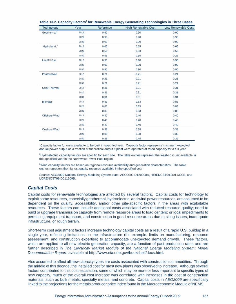
Capital CostsCapital costs for renewable technologies are affected by several factors. Capital costs for technology toexploit some resources, especially geothermal, hydroelectric, and wind power resources, are assumed to bedependent on the quality, accessibility, and/or other site-specific factors in the areas with exploitableresources. These factors can include additional costs associated with reduced resource quality; need tobuild or upgrade transmission capacity from remote resource areas to load centers; or local impediments topermitting, equipment transport, and construction in good resource areas due to siting issues, inadequateinfrastructure, or rough terrain.
Short-term cost adjustment factors increase technology capital costs as a result of a rapid U.S. buildup in asingle year, reflecting limitations on the infrastructure (for example, limits on manufacturing, resourceassessment, and construction expertise) to accommodate unexpected demand growth. These factors,which are applied to all new electric generation capacity, are a function of past production rates and arefurther described in The Electricity Market Module of the National Energy Modeling System: ModelDocumentation Report, available at http://www.eia.doe.gov/bookshelf/docs.html.
Also assumed to affect all new capacity types are costs associated with construction commodities. Throughthe middle of this decade, the installed cost for most new plants was observed to increase. Although severalfactors contributed to this cost escalation, some of which may be more or less important to specific types ofnew capacity, much of the overall cost increase was correlated with increases in the cost of constructionmaterials, such as bulk metals, specialty metals, and concrete. Capital costs in AEO2009 are specificallylinked to the projections for the metals producer price index found in the Macroeconomic Module of NEMS.
Energy Information Administration/Assumptions to the Annual Energy Outlook 2009 157
Technology Year Reference High Renewable Cost Low Renewable CostGeothermal2 2012 0.90 0.90 0.90
2020 0.90 0.90 0.90
2030 0.90 0.90 0.90
Hydrolectric2 2012 0.65 0.65 0.65
2020 0.56 0.53 0.56
2030 0.55 0.55 0.26
Landfill Gas 2012 0.90 0.90 0.90
2020 0.90 0.90 0.90
2030 0.90 0.90 0.90
Photovoltaic 2012 0.21 0.21 0.21
2020 0.21 0.21 0.21
2030 0.21 0.21 0.21
Solar Thermal 2012 0.31 0.31 0.31
2020 0.31 0.31 0.31
2030 0.31 0.31 0.31
Biomass 2012 0.83 0.83 0.83
2020 0.83 0.83 0.83
2030 0.83 0.83 0.83
Offshore Wind3 2012 0.40 0.40 0.40
2020 0.40 0.40 0.40
2030 0.40 0.40 0.40
Onshore Wind3 2012 0.38 0.38 0.38
2020 0.38 0.38 0.38
2030 0.46 0.45 0.39
Table 13.2. Capacity Factors1 for Renewable Energy Generating Technologies in Three Cases
1Capacity factor for units available to be built in specified year. Capacity factor represents maximum expectedannual power output as a fraction of theoretical output if plant were operated at rated capacity for a full year.2Hydroelectric capacity factors are specific for each site. The table entries represent the least-cost unit available inthe specified year in the Northwest Power Pool region.3Wind capacity factors are based on regional resource availability and generation characteristics. The tableentries represent the highest quality resource available in the specified year.
Source: AEO2009 National Energy Modeling System runs: AEO2009.D120908A, HIRENCST09.D011309B, andLORENCST09.D011509B.

Independent of the other two factors, capital costs for all electric generation technologies, includingrenewable technologies, are assumed to decline as a function of growth in installed capacity for eachtechnology.
For a description of NEMS algorithms lowering generating technologies’ capital costs as more units enterservice (learning), see “Technological Optimism and Learning” in the EMM chapter of this report. A detaileddescription of the RFM is provided in the EIA publication, Renewable Fuels Module of the National EnergyModeling System, Model Documentation 2005, DOE/EIA-M069(2005) (Washington, DC, 2005).
Solar Electric SubmoduleBackgroundThe Solar Electric Submodule currently includes both concentrating solar power (thermal) andphotovoltaics, including two solar technologies: 50 megawatt central receiver (power tower) solar thermal(ST) and 5 megawatt single axis tracking-flat plate photovoltaic (PV) technologies. PV is assumed availablein all thirteen EMM regions, while ST is available only in the six Western regions with the arid atmosphericconditions that result in the most cost-effective capture of direct sunlight. Capital costs for both technologiesare determined by EIA using multiple sources, including public reports of recent solar thermal capacityadditions. Most other cost and performance characteristics for ST are obtained or derived from the August 6,1993, California Energy Commission memorandum, Technology Characterization for ER 94; and, for PV,from the Electric Power Research Institute, Technical Assessment Guide (TAG) 1993. In addition, capacityfactors are obtained from information provided by the National Renewable Energy Laboratory (NREL).
Assumptions
• Capacity factors for solar technologies are assumed to vary by time of day and season of the year,such that nine separate capacity factors are provided for each modeled region, three for time of dayand for each of three broad seasonal groups (summer, winter, and spring/fall). Regional capacityfactors vary from national averages. The current reference case solar thermal annual capacity factorfor California, for example, is assumed to average 40 percent; California’s current reference case PVcapacity factor is assumed to average 24.6 percent.
• Because solar technologies are more expensive than other utility grid-connected technologies, earlypenetration will be driven by broader economic decisions such as the desire to become familiar with anew technology, environmental considerations, and the availability of limited Federal subsidies.Minimal early years’ penetration is included by EIA as “floor” additions to new generating capacity(see “Supplemental and Floor Capacity Additions” below).
• Solar resources are well in excess of conceivable demand for new capacity; energy supplies areconsidered unlimited within regions (at specified daily, seasonal, and regional capacity factors).Therefore, solar resources are not estimated in NEMS. In the seven regions where ST technology isnot modeled, the level of direct, normal insolation (the kind needed for that technology) is assumed tobe insufficient to make that technology commercially viable through 2030.
• NEMS represents the Energy Policy Act of 1992 (EPACT92) permanent 10-percent investment taxcredit (ITC) for solar electric power generation by tax-paying entities. In addition, the current30-percent ITC scheduled to expire at the end of 2016, is also represented to qualifying new capacityinstallations.
Wind-Electric Power SubmoduleBackgroundBecause of limits to windy land areas, wind is considered a finite resource, so the submodule calculatesmaximum available capacity by Electricity Market Module Supply Regions. The minimum economicallyviable average wind speed is about 14 mph, and wind speeds are categorized by annual average windspeed based on a classification system originally from the Pacific Northwest Laboratory. The RFM trackswind capacity (megawatts) by resource quality, and costs within a region and moves to the next best windresource when one category is exhausted. For AEO2009, wind resource data on the amount and quality of
158 Energy Information Administration/Assumptions to the Annual Energy Outlook 2009

wind per EMM region come from the National Renewable Energy Laboratory2 The technologicalperformance, cost, and other wind data used in NEMS are derived by EIA from available data and fromavailable literature.3 Maximum wind capacity, capacity factors, and incentives are provided to the EMM forcapacity planning and dispatch decisions. These form the basis on which the EMM decides how muchpower generation capacity is available from wind energy. The fossil-fuel heat rate equivalents for wind areused for energy consumption calculation purposes only.
Assumptions
• Only grid-connected (utility and nonutility) generation is included. Projections for distributed windgeneration are included in the commercial and residential modules.
• In the wind submodule, wind supply costs are affected by three modeling measures: addressing (1)average wind speed, (2) distance from existing transmission lines, and (3) resource degradation,transmission network upgrade costs, and market factors.
• Available wind resource is reduced by excluding all windy lands not suited for the installation of windturbines because of: excessive terrain slope (greater than 20 percent); reservation of land fornon-intrusive uses (such as National Parks, wildlife refuges, and so forth); inherent incompatibilitywith existing land uses (such as urban areas, areas surrounding airports and water bodies, includingoffshore locations); insufficient continguous windy land to support a viable wind plant (less than 5square kilometers of windy land in a 100 square kilometer area). Half of the wind resource located onmilitary reservations, U.S. Forest Service land, state forested land, and all non-ridge-crest forestareas are excluded from the available resource base to account for the uncertain ability to siteprojects at such locations. These assumptions are detailed in the Draft Final Report to EIA onIncorporation of Existing Validated Wind Data into NEMS, November 2003.
• Capital costs for wind technologies are assumed to increase in response to (1) declining naturalresource quality, such as terrain slope, terrain roughness, terrain accessibility, wind turbulence, windvariability, or other natural resource factors, as the best sites are utilized (2) increasing cost ofupgrading existing local and network distribution and transmission lines to accommodate growingquantities of remote wind power, and (3) market conditions, such as the increasing costs ofalternative land uses, including aesthetic or environmental reasons. Capital costs are leftunchanged for some initial share, then increased 20, 50, 100 percent, and finally 200 percent, torepresent the aggregation of these factors.
• Proportions of total wind resources in each category vary by EMM region. For all thirteen EMMregions combined, 1.3 percent of windy land is available with no cost increase, 5.4 percent isavailable with a 20 percent cost increase, 11.2 percent is available with a 50 percent cost increase,27.3 percent is available with a 100 percent cost increase, and almost 54.8 percent of windy land isassumed to be available with a 200 percent cost increase.
• Depending on the EMM region, the cost of competing fuels, and other factors, wind plants can be builtto meet system capacity requirements or as a “fuel saver” to displace generation from existingcapacity. For wind to penetrate as a fuel saver, its total capital and fixed operations and maintenancecosts minus applicable subsidies must be less than the variable operating costs, including fuel, of theexisting (non-wind) capacity. When competing in the new capacity market, wind is assigned acapacity credit that declines based on its estimated contribution to regional reliability requirements.
• Because of downwind turbulence and other aerodynamic effects, the model assumes an averagespacing between turbine rows of 5 rotor diameters and a lateral spacing between turbines of 10 rotordiameters. This spacing requirement determines the amount of power that can be generated fromwind resources, about 6.5 megawatts per square kilometer of windy land, and is factored intorequests for generating capacity by the EMM.
• Capacity factors are assumed to increase to a 46 percent in the best wind class resulting from tallertowers, more reliable equipment, and advanced technologies. Capacity factors for each wind classare calculated as a function of overall wind market growth. The capacity factors are assumed to be
Energy Information Administration/Assumptions to the Annual Energy Outlook 2009 159

limited to about 48 percent for an average Class 6 site. As better wind resources are depleted,capacity factors are assumed to go down. By 2030, the typical wind plant build will have a somewhatlower capacity factor than those found in the best wind resource area.
• AEO2009 does not allow plants constructed after 2009 to claim the Federal Production Tax Credit(PTC), a 2 cent per kilowatt-hour tax incentive that is set to expire on December 31, 2009. Windplants are assumed to depreciate capital expenses using the Modified Accelerated Cost RecoverySchedule with a 5-year tax life.
Offshore wind resources are represented as a separate technology from onshore wind resources. Offshoreresources are modeled with a similar model structure as onshore wind. However, because of the uniquechallenges of offshore construction and the somewhat different resource quality, the assumptions withregard to capital cost, learning-by-doing cost reductions, and variation of resource exploitation costs andperformance differ significantly from onshore wind.
• Like onshore resources, offshore resources are assumed to have an upwardly sloping supply curve,in part influenced by the same factors that determine the onshore supply curve (such as distance toload centers, environmental or aesthetic concerns, variable terrain/seabed) but also explicitly bywater depth.
• Because of the more difficult maintenance challenge offshore, performance for given annual averagewind power density level is assumed to be somewhat reduced by reduced turbine availability.Offsetting this, however, is the availability of resource areas with higher overall power density than isassumed available onshore. Capacity factors for offshore are limited to be about 50 percent for aClass 7 site.
• Cost reductions in the offshore technology result in part from learning reductions in onshore windtechnology as well as from cost reductions unique to offshore installations, such as foundation designand construction techniques. Because offshore technology is significantly less mature than onshorewind technology, offshore-specific technology learning occurs at a somewhat faster rate thanon-shore technology.
Geothermal-Electric Power SubmoduleBackgroundThe Geothermal-Electric Submodule (GES) estimates the generating capacity and output potential of 89hydrothermal sites in the Western United States. This estimation is based on two studies: New GeothermalSite Identification and Qualification, prepared by GeothermEx, Inc for the California Public UtilityCommission, and Western Governors’ Association Geothermal Task Force Report, which was co-authoredby several geothermal experts from the public and private sectors. These studies focus on geothermalresources with confirmed temperatures greater than 100 Celsius, which is generally considered thethreshold for economically feasible conventional development. While EIA had previously distinguishedbetween binary and dual flash technologies, this is no longer an essential component of cost estimates.Instead, these studies incorporate expected power plant cost and performance based on each confirmedresource temperature. This enables greater projection precision relative to a static choice between twotechnologies. All plants are assumed to operate at 90 percent capacity factor. Enhanced GeothermalSystems (EGS), such as hot dry rock, are not included as potential resources since this technology is still indevelopment and is not expected to be in significant commercial use within the projection horizon. As part ofEPACT 2005, the U.S. Geological Survey recently completed its comprehensive review of all domestichydrothermal resources. While the final data show overall capacity estimates similar to the ones presented in theabove-mentioned studies, there are undoubtedly distinctions in individual site characterizations and methodsused for estimating capacity. Although the final aggregate data has been released, the assumptions andindividual site estimates have not. Therefore, the data will not be incorporated into the AEO until 2010.
The two studies off of which EIA estimates are based maintain separate capital cost components for eachsite’s development. The GeothermEx study divided individual site costs into four components: exploration,confirmation, development, and transmission. Site exploration is a small component of aggregate costs,oftentimes being zero. Confirmation and transmission costs may be significant, however the vast majority of
160 Energy Information Administration/Assumptions to the Annual Energy Outlook 2009

capital costs are classified under site development which includes power plant construction. The WGAreport, which was used to estimate geothermal potential outside of the GeothermEx database region, did notprovide site specific, separate capital cost components. However, it did provide some sites with two levels ofcapital costs, meaning a portion of the resource could be developed at a lower cost than the remainingpotential. Therefore, EIA maintained two categories of site specific capital development costs, with a costpremium placed on some sites beyond their most economic resource. Site specific operation andmaintenance costs are also included in the submodule. As a result of revised supply estimations, the annualsite build limit has been relaxed but still remains. Geothermal development is limited to 25 MW of generatingcapacity until 2010, when the 50 MW limit goes into effect for the remainder of the projection period.
Assumptions
• Existing and identified planned capacity data are obtained directly by the EMM from Forms EIA-860A(utilities) and EIA-860B (nonutilities) and from supplemental additions (See Below).
• The permanent investment tax credit of 10 percent available in all projection years based on theEPACT applies to all geothermal capital costs, except through December 2010 when the 2-centproduction tax credit is available to this technology and is assumed chosen instead.
• Plants are not assumed to retire unless their retirement is reported to EIA. Geysers units are notassumed to retire but instead are assigned the 35 percent capacity factors reported to EIA reflectingtheir reduced performance in recent years.
• Capital and operating costs vary by site and year; values shown in Table 8.3 in the EMM chapter areindicative of those used by EMM for geothermal build and dispatch decisions.
Biomass Electric Power SubmoduleBackgroundBiomass consumed for electricity generation is modeled in two parts in NEMS. Capacity in the woodproducts and paper industries, the so-called captive capacity, is included in the industrial sector module ascogeneration. Generation by the electricity sector is represented in the EMM, with capital and operatingcosts and capacity factors as shown in Table 8.2 in the EMM chapter, as well as fuel costs, being passed tothe EMM where it competes with other sources. Fuel costs are provided in sets of regional supply schedules.Projections for ethanol are produced by the Petroleum Market Module (PMM), with the quantities of biomassconsumed for ethanol decremented from, and prices obtained from, the EMM regional supply schedules.
Assumptions
• Existing and planned capacity data are obtained from Form EIA-860.
• The conversion technology represented, upon which the costs in Table 8.3 in the EMM chapter arebased, is an advanced gasification-combined cycle plant that is similar to a coal-fired gasifier. Costsin the reference case were developed by EIA to be consistent with coal gasifier costs. Short-termcost adjustment factors are used.
• Biomass cofiring can occur up to a maximum of 15 percent of fuel used in coal-fired generatingplants.
Fuel supply schedules are a composite of four fuel types: forestry materials, wood residues, agriculturalresidues and energy crops. Energy crop data are presented in yearly schedules from 2010 to 2030 incombination with the other material types for each region. The forestry materials component is made up oflogging residues, rough rotten salvageable dead wood, and excess small pole trees.4 The wood residuecomponent consists of primary mill residues, silvicultural trimmings, and urban wood such as pallets,construction waste, and demolition debris that are not otherwise used.5 Agricultural residues are wheatstraw, corn stover, and a number of other major agricultural crops.6 Energy crop data are for hybrid poplar,
Energy Information Administration/Assumptions to the Annual Energy Outlook 2009 161

willow, and switchgrass grown on crop land, pasture land, or on Conservation Reserve Program lands. InAEO2009, agricultural residues and energy crops are combined into a single "agricultural sector."7 Themaximum amount of resources in each supply category is shown in Table 13.3.
Landfill-Gas-to-Electricity SubmoduleBackgroundLandfill-gas-to-electricity capacity competes with other technologies using supply curves that are based onthe amount of “high”, “low”, and “very low” methane producing landfills located in each EMM region. Anaverage cost-of-electricity for each type of landfill is calculated using gas collection system and electricitygenerator costs and characteristics developed by EPA’s “Energy Project Landfill Gas Utilization Software”(E-PLUS).8
Assumptions
• Gross domestic product (GDP) and population are used as the drivers in an econometric equationthat establishes the supply of landfill gas.
• Recycling is assumed to account for 35 percent of the total waste stream by 2005 and 50 percent by2010 (consistent with EPA’s recycling goals).
• The waste stream is characterized into three categories: readily, moderately, and slowlydecomposable material.
• Emission parameters are the same as those used in calculating historical methane emissions in theEIA’s Emissions of Greenhouse Gases in the United States 2003.9
162 Energy Information Administration/Assumptions to the Annual Energy Outlook 2009
Coal DemandRegion States
AgriculturalSector
Forestry ResidueUrban Wood Waste/Mill Residue
Total1
1 CT, MA, ME, NH, RI, VT 165 158 15 339
2 NY, PA, NJ 277 167 59 503
3 WV, MD, DC, DE, VA, NC, SC 436 426 56 918
4 GA, FL 239 265 47 551
5 OH 348 37 16 402
6 IN, IL, MI, WI 1209 190 47 1,446
7 KY, TN 497 152 30 679
8 AL, MS 357 326 19 702
9 MN, IA, ND, SD, NE, MO, KS 2294 155 28 2,477
10 TX, LA, OK, AR 728 378 57 1,163
11 MT, WY, ID 197 100 25 322
12 CO, UT, NV 209 70 7 285
13 AZ, NM 168 45 7 220
14 AK, HI, WA, OR, CA 226 429 83 738
Table 13.3. 2020 Maximum U.S. Biomass Resources, by Coal Demand Region and Type (Trillion Btu)
1May include rounding error.
Sources: Urban Wood Wastes: Antares Group Inc., Biomass Residue Supply Curves for the U.S (updated), prepared for theNational Renewable Energy Laboratory, June 1999; Agricultural residues, energy crops, and forestry residues from theUniversity of Tennessee Department of Agricultural Economics POLYSIS model, May 2008.

• The ratio of “high”, “low”, and “very low” methane production sites to total methane production iscalculated from data obtained for 156 operating landfills contained in the Government AdvisoryAssociates METH2000 database.10
• Cost-of-electricity for each site was calculated by assuming each site to be a 100-acre by 50-footdeep landfill and by applying methane emission factors for “high”, “low”, and “very low” methaneemitting wastes.
Conventional HydroelectricityThe conventional hydroelectricity submodule represents U.S. potential for new conventional hydroelectriccapacity 1 megawatt or greater from new dams, existing dams without hydroelectricity, and from addingcapacity at existing hydroelectric dams. Summary hydroelectric potential is derived from reported lists ofpotential new sites assembled from Federal Energy Regulatory Commission (FERC) license applicationsand other survey information, plus estimates of capital and other costs prepared by the Idaho NationalEngineering and Environmental Laboratory (INEEL).11 Annual performance estimates (capacity factors)were taken from the generally lower but site specific FERC estimates rather than from the general estimatesprepared by INEEL, and only sites with estimated costs 10 cents per kilowatthour or lower are included in thesupply. Pumped storage hydro, considered a nonrenewable storage medium for fossil and nuclear power, isnot included in the supply; moreover, the supply does not consider offshore or in-stream hydro, efficiency oroperational improvements without capital additions, or additional potential from refurbishing existinghydroelectric capacity.
In the hydroelectricity submodule, sites are first arrayed by NEMS region from least to highest cost perkilowatthour. For any year’s capacity decisions, only those hydroelectric sites whose estimated levelizedcosts per kilowatthour are equal to or less than an EMM determined avoided cost (the least cost of othertechnology choices determined in the previous decision cycle) are submitted. Next, the array ofbelow-avoided cost sites is parceled into three increasing cost groups, with each group characterized by theaverage capacity-weighted cost and performance of its component sites. Finally, the EMM receives from theconventional hydroelectricity submodule the three increasing-cost quantities of potential capacity for eachregion, providing the number of megawatts potential along with their capacity-weighted average overnightcapital cost, operations and maintenance cost, and average capacity factor. After choosing from the supply,the EMM informs the hydroelectricity submodule, which decrements available regional potential inpreparation for the next capacity decision cycle.
Legislation and Regulations
Energy Policy Act of 1992 (EPACT92) and 2005 (EPACT05)The RFM includes the investment and energy production tax credits codified in the Energy Policy Act of 1992(EPACT 92) as amended. The investment tax credit established by EPACT 92 provides a credit to Federalincome tax liability worth 10 percent of initial investment cost for a solar, geothermal, or qualifying biomassfacility. This credit was raised to 30 percent through 2016 for some solar projects and extended to residentialprojects. This change is reflected in the utility, commercial and residential modules. The production taxcredit, as established by EPACT 92, applied to wind and certain biomass facilities. As amended, it providesa 2 cent tax credit for every kilowatt-hour of electricity produced for the first 10 years of operation for a windfacility constructed by December 31, 2009 or by December 31, 2010 for other eligible facilities. The value ofthe credit, originally 1.5 cents, is adjusted annually for inflation. With the various amendments, theproduction tax credit is available for electricity produced from qualifying geothermal, animal waste, certainsmall-scale hydroelectric, landfill gas, municipal solid waste, and additional biomass resources. Wind,poultry litter and geothermal, and "closed loop"12 biomass resources receive a 2 cent tax credit for the first 10years of facility operations. All other renewable resources receive a 1 cent tax credit for the first 10 years offacility operations. EIA assumes that biiomass facilities obtaining the PTC will use "open-loop" fuels, as"closed-loop" fuels are assumed to be unavailable and/or too expensive for widespread use during theperiod that the tax credit is available. The investment and production tax credits are exclusive of one another,and may not both be claimed for the same geothermal facility (which is eligible to receive either).
Energy Information Administration/Assumptions to the Annual Energy Outlook 2009 163

Alternative Renewable Cases
Renewable Technology CasesTwo cases examine the effect on energy supply using alternative assumptions for cost and performance ofnon-hyrdo, non-landfill gas renewable energy technologies. The High Renewable Cost case examines theeffect if technology costs were to remain at current levels. The Low Renewable Cost case examines theeffect if technology energy costs were reduced by 2030 to 25 percent below Reference case values.
The High Renewable Cost case does not allow “learning-by-doing” effects to reduce the capital cost ofbiomass, geothermal, solar, or wind technologies or to improve wind capacity factor beyond 2009 levels.The construction of the first four units of biomass integrated gasification combined cycle units are stillassumed to reduce the technological optimism factor associated with this technology. Although the cost ofbiiomass fuels is assumed to remain the same in this case as in the Reference case, this case assumes thatno energy crops will be available through 2030, consistent with the "frozen technology" assumptions for theother technologies. All other parameters remain the same as in the Reference case.
The Low Renewable Cost case assumes that the non-hydro, non-landfill gas renewable technologies areable to reduce their overall cost-of-energy produced in 2030 by 25 percent from the Reference case.Because the cost of supply of renewable resources is assumed to increase with increasing utilization (that is,the renewable resource supply curves are upwardly sloping), the cost reduction is achieved by targeting thereduction on the “marginal” unit of supply for each technology in 2030 for the Reference case (that is, thenext resource available to be utilized in the Reference case in 2030). This has the effect of reducing costs forthe entire supply (that is, shifting the supply curve downward by 25 percent). As a result of the overallreduction in costs, more supply may be utilized, and a unit from higher on the supply curve may result inbeing the marginal unit of supply. Thus the actual market-clearing cost-of-energy for a given renewabletechnology may not differ by much from the Reference case, although that resource contributes more energysupply than in the Reference case. These cost reductions are achieved gradually through "learning-by-doing”, and are only fully realized by 2030.
For wind, biomass, geothermal, and solar technologies, this cost reduction is achieved by a reduction inovernight capital costs sufficient to achieve the 10 percent targeted reduction in cost-of-energy. As a result,the supply of biomass fuel is increased by 10 percent at every price level. For geothermal, the capital cost ofthe lowest-cost site available in the year 2005 is reduced such that if it were available for construction in2030, it would have a 10 percent lower cost-of-energy in the High Renewable case than the cost-of-energy itwould have in 2030 were it available for construction in the Reference case. For solar technologies (bothphotovoltaic and solar thermal power), the resource is assumed to be unlimited and the reductions incost-of-energy are achieved strictly through capital cost reduction. Biomass prices is assumed to be reduced25 percent by 2030 for a given quantity of fuel supplied. Other assumptions within NEMS are unchangedfrom the Reference case.
For the Low Renewable Cost case, demand-side improvements are also assumed in the renewable energytechnology portions of residential and commercial buildings, industrial processes, and refinery fuelsmodules. Details on these assumptions can be found in the corresponding sections of this report.
State RPS Programs
EIA represents various state-level policies generally referred to as Renewable Portfolio Standards (RPS).These policies vary significantly among states, but typically require the addition of renewable generation tomeet a specified share of state-wide generation. Any non-discretionary limitations on meeting thegeneration or capacity target are modeled to the extent possible. However, because of the complexity of thevarious requirements, the regional target aggregation (described below), and nature of some of thelimitations (also described below), measurement of compliance is assumed to be approximate.
For the AEO2009, regional renewable generation targets were estimated using the renewable generationtargets in each state within the region. In many cases, regional boundaries intersect state boundaries; inthese cases states were assigned to be within a single region, based on EIA expert judgment of factors suchas predominant load locations and location of renewable resources eligible for that state’s RPS program.
164 Energy Information Administration/Assumptions to the Annual Energy Outlook 2009

Using state-level RPS compliance schedules and preliminary estimates of projected sales growth, EIAestimated the amount of renewable generation required in each state within a region. Required generation ineach state was then summed to the regional level for each year, and a regional renewable generation shareof total sales was determined, as shown in Table 13.5.
Only targets with established enforcement provisions or established state funding mechanisms wereincluded in the calculation; goals, provisional RPS requirements, or requirements lacking establishedfunding were not included. The California and New York programs require state funding, and theseprograms are assumed to be complied with only to the extent that state funding allows. Complianceenforcement provisions vary significantly among states and most states have established procedures forwaiving compliance through the use of “alternative compliance” payments, penalty payments, discretionary
regulatory waivers, or retail price impact limits. Because of the variety of mechanisms, even within a givenelectricity market region, these limits are not modeled.
Supplemental and Floor Capacity Additions
For AEO2009, has estimated near-term additions of renewable operating capacity. These estimates arebased on a number of public and proprietary databases of new project capacity, and provide a plant-specificaccounting of new capacity in 2008 and subsequent years. Because of the significant growth in this sectorduring 2008 specific plants are not listed Table 13.6.
Energy Information Administration/Assumptions to the Annual Energy Outlook 2009 165
Region1 2015 2025 2030ECAR 3.0% 5.7% 5.7%
ERCOT 5.0% 5.0% 5.0%
MAAC 10.1% 15.4% 15.4%
MAIN 6.7% 15.3% 15.3%
MAPP 8.5% 11.1% 11.1%
NY2 18.3% 18.3% 18.3%
NE 9.3% 12.6% 12.6%
FL 0.0% 0.0% 0.0%
STV 0.9% 1.9% 1.9%
SPP 0.0% 0.0% 0.l0%
NWP 7.3% 13.0% 13.0%
RA 4.2% 6.9% 6.9%
CNV3 * * *
Table 13.5. Aggregate Regional RPS Requirements
1 See chapter on the electricity Market Module for a map of the electricity regions2California is not projected to meet RPS targets because of funding limitations. EIA projects that currently authorized funds willsupport the addition of approximately 900 MW of additional renewable capacity through 2011.

166 Energy Information Administration/Assumptions to the Annual Energy Outlook 2009
Geothermal Hydro MSW Solar PV Solar Thermal Biomass Wind Total
2008 8.98 1 8692.45 8702.43
2009 1 895.25 896.25
2010 1
Table 13.6. Planned U.S. Central Station Generating Capacity Using Renewable Resources for 2004 and Beyond1
Sources: EIA contact with project developers, American Wind Energy Association, Energy Velocity ™ Database.

[1] For a comprehensive description of each submodule, see Energy Information Administration, Office ofIntegrated Analysis and Forecasting, Model Documentation, Renewable Fuels Module of the NationalEnergy Modeling System, DOE/EIA-M069(2005), (Washington, DC, March 2005).
[2] Revising the Long Term Multipliers in NEMS: Quantifying the Incremental Transmission Costs Due toWind Power, Report to EIA from Princeton Energy Resources International, LLC. May 2007.
[3] Wiser, Ryan and Mark Bollinger. Annual Report on U.S. Wind Power Installation, Cost, and PerformanceTrends: 2006. U.S. Department of Energy, Office of Energy Efficiency and Reneweable Energy. May 2007.
[4] United States Department of Agriculture, U.S. Forest Service, "Forest Resources of the United States,1992", General Technical Report RM-234, (Fort Collins CO, June 1994).
[5] Antares Group Inc., "Biomass Residue Supply Curves for the U.S (updated)", prepared for the NationalRenewable Energy Laboratory, June 1999.
[6] Walsh, M.E., et.al., Oak Ridge National Laboratory, "The Economic Impacts of Bioenergy CropProduction on U.S. Agriculture", (Oak Ridge, TN, May 2000), http://bioenergy.ornl.gov/papers/wagin/index.html.
[7] Graham, R.L., et.al., Oak Ridge National Laboratory, “The Oak Ridge Energy Crop County LevelDatabase”, (Oak Ridge TN, December, 1996).
[8] U.S. Environmental Protection Agency, Atmospheric Pollution Prevention Division, Energy ProjectLandfill Gas Utilization Software (E-PLUS) Version 1.0, EPA-430-B-97-006 (Washington, DC, January1997).
[9] Energy Information Administration, "Emissions of Greenhouse Gases in the United States 2003",DOE/EIA-0573(2003) (Washington, DC, December 2004).
[10] Governmental Advisory Associates, Inc., METH2000 Database, Westport, CT, January 25, 2000.
[11] Douglas G. Hall, Richard T. Hunt, Kelly S. Reeves, and Greg R. Carroll, Idaho National Engineering andEnvironmental Laboratory, "Estimation of Economic Parameters of U.S. Hydropower Resources"INEEL/EXT-03-00662 (Idaho Falls, Idaho, June 2003).
[12] Closed-loop biomass are crops produced explicitly for energy production. Open-loop biomass aregenerally wastes or residues that are a byproduct of some other process, such as crops grown for food,forestry, landscaping, or wood milling
Energy Information Administration/Assumptions to the Annual Energy Outlook 2009 167
Notes and Sources


Appendix A: Handling of Federal andSelected State Legislation and
Regulation in the Annual Energy Outlook

170 Energy Information Administration/Assumptions to the Annual Energy Outlook 2009
Appendix A: Handling of Federal and Selected State Legislation and Regulation in the Annual Energy Outlook
Legislation Brief Description AEO Handling Basis
Residential Sector
A. National Appliance Energy Conservation Act of 1987
Requires Secretary of Energy toset minimum efficiencystandards for 10 appliancecategories.
Included for categoriesrepresented in the AEOresidential sector forecast.
a. Room Air Conditioners Current standard of 9.8 EER Federal Register Notice of FinalRulemaking.
b. Other Air Conditioners (<5.4 tons)
Current standard 10 SEET forcentral air conditioners and heatpumps, increasing to 13 SEERin 2006.
Federal Register Notice of FinalRulemaking.
c. Water Heaters Electric: Current standard .90EF. Gas: Current standard .59EF.
Federal Register Notice of FinalRulemaking.
d. Refrigerators/Freezers kWh/yr
Current standard of .51 Federal Register Notice of FinalRulemaking.
e. Dishwashers Current standard of .46 EF. Federal Register Notice of FinalRulemaking.
f. Fluorescent Lamp Ballasts
Current standard of .90 powerfactor
Federal Register Notice of FinalRulemaking.
g. Clothes Washers Current standard of 1.18 EF,increasing to 1.04 MEF in 2004,further increasing to 1.26 MEFin 2007.
Federal Register Notice of FinalRulemaking.
h. Furnaces Standard set at 78 AFUE forgas and oil furnaces.
Federal Register Notice of FinalRulemaking.
i. Clothes Dryers Gas: Current standard 2.67 EF.Electric: Current standard 3.01EF. The increase in MEF forclothes washers furtherincreases the de facto standardfor clothes dryers due to betterextraction of water from clothesin washing process.
Federal Register Notice of FinalRulemaking.
B. Energy Policy Act of 1992 (EPACT92)
a. Building Codes For the IECC 2006, specifieswhole house efficiencyminimums.
Assumes that all States adoptthe IECC 2006 code by 2017.
Trend of States adoption tocodes, allowing for lead timesfor enforcement and buildercompliance.
b. Energy-Efficient Mortgages
Allow homeowners to qualify forhigher loan amounts if thehome is energy-efficient, asscored by HERS.
Efficiency of equipmentrepresented in technologychoice parameters. Efficiencyof shell represented in HVACchoice.
No way to separate out thesepurchases from others.Assumes historical effect in theforecast, with cost-reducinglearning in the shell portion ofHVAC choice.
C. Energy Policy Act of 2005 (EPACT05)
a. Torchiere Lamp Standard
Sets 190 watt bulb limit in 2006. EPACT05.
b. Ceiling Fan Light Kit Standard
Ceiling fans must be shippedwith compact fluorescent bulbsor use no more than 190 wattsper fixture in 2007.
Reduce lighting electricityconsumption by appropriateamount.
Number of ceiling fanshipments and estimated kWhsavings per unit determineoverall savings.

171Energy Information Administration/Assumptions to the Annual Energy Outlook 2009
Legislation Brief Description AEO Handling Basis
c. Dehumidifier Standard Sets standard for dehumidifiersin 2007 and 2012.
Reduce miscellaneouselectricity consumption byappropriate amount.
Number of dehumidifiershipments and estimated kWhsavings per unit determineoverall savings.
d. Energy-Efficient Equipment Tax Credit
Purchasers of certain energy-efficient equipment can claimtax credits in 2006 and 2007.
Reduce cost of applicableequipment by specified amount.
EPACT05.
e. New Home Tax Credit Builders receive $1000 or$2000 tax credit if they buildhomes 30 or 50 percent betterthan code in 2006 and 2007.
Reduce shell package cost forthese homes by specifiedamount.
Cost reductions to consumersare assumed to be 100 percentof the builder’s tax credit.
f. Energy-Efficient Appliance Tax Credit
Producers of energy-efficientrefrigerators, dishwashers, andclothes washers receive taxcredits for each unit theyproduce that meets certainefficiency specifications.
Assume the cost savings arepassed on to the consumer,reducing the price of theappliance by the specifiedamount.
Cost reductions to consumersare assumed to be 100 percentof the producer’s tax credit.
D. Energy Independence and Security Act of 2007 (EISA 2007)
a. General Service Incandescent Lamp Standard
Require less wattage for bulbsin 2012-2014 and 2020.
reduce wattage for new bulbsby 28 percent in 2013 and 67percent in 2020.
EISA 2007
b. Dehumidifier Standard Updates EPACT 2005standard.
Reduce miscellaneouselectricity consumption byappropriate amount.
Increase savings estimated forEPACT 2005 by appropriateamount.
c. Boiler Standard Sets standards for boilers in2013.
Require new purchases ofboilers to meet the standard.
EISA 2007
d. Dishwasher Standard Sets standards for dishwashersin 2010.
Require new purchases ofdishwashers to meet thestandard by 2010.
EISA 2007
e. External Power Supply Standard
Sets standards for externalpower supplies in 2008
Reduce miscellaneouselectricity consumption byappropriate amount.
Number of shipments andestimated kWh savings per unitdetermine overall savings.
f. Manufactured Housing Code
Require manufactured homesto meet latest IECC in 2011.
Require that all manufacturedhomes shipped after 2011 meetthe IECC 2006
EISA 2007
E. Energy Improvement and Extension Act of 2008 (EIEA 2008)
a. Energy-Efficient Equipment Tas Credit
Purchasers of certain energy-efficient equipment can claimtax credits through 2016
Reduce the cost of applicableequipment by specified amount
EIEA 2008
b. Energy-Efficient Appliance Tax Credit
Producers of energy-efficientrefrigerators, clothes washers,and dishwashers receive taxcredits for each unit theyproduce that meets certainefficiency specifications, subjectto an annual cap.
Assume the cost savings arepassed on to the consumer,reducing the price of theappliance by the specifiedamount.
Cost reductions to consumersare assumed to be 100% of theproducer’s tax credit.
Commercial Sector
A. National Appliance Energy Conservation Act of 1987
Requires Secretary of Energy toset minimum efficiencystandards for 10 appliancecategories.
Included for categoriesrepresented in the AEOcommercial sector forecast.
a. Room Air Conditioners Current standard of 9.8 EER Federal Register Notice of FinalRulemaking.
b. Other Residential-size Air Conditioners (<5.4 tons)
Current standard 10 SEER forcentral air conditioning and heatpumps, increasing to 13 SEERin 2006.
Federal Register Notice of FinalRulemaking.

Legislation Brief Description AEO Handling Basis
172 Energy Information Administration/Assumptions to the Annual Energy Outlook 2009
c. Fluorescent LampBallasts
Current standard if .90 powerfactor and minimum efficacyfactor for F40 and F96 lampsbased on lamp size andwattage, increasing to higherefficacy factor in 2005 that limitspurchases to electronicballasts.
Federal Register Notice of FinalRulemaking.
B. Energy Policy Act of 1992 (EPACT92)
a. Buildings Codes Incorporated in commercialbuilding shell assumptions.Efficiency of new relative toexisting shell represented inshell efficiency indices.Assume shell efficiencyimproves 5 and 7 percent by2030 for existing buildings andnew construction, respectively.
Based on Science ApplicationsInternational Corporationcommercial shell indices for2003 developed for EIA in2008.
b. Window labeling Designed to help consumersdetermine which windows aremore energy efficient.
Incorporated in commercialbuilding shell assumptions.Efficiency of new relative toexisting shell represented Ishell efficiency indices.Assume shell efficiencyimproves 5 and 7 percent by2030 for existing buildings andnew construction, respectively.
Based on Science ApplicationsInternational Corporationcommercial shell indices for2003 developed for EIA in2008.
c. Commercial Furnaces and Boilers
Gas-fired furnaces and boilers:Current standard is 0.80thermal efficiency. Oilfurnaces and boilers: Currentstandard is 0.81 thermalefficiency for furnaces, 0.83thermal efficiency for boilers.
Public Law 102-486:EPACT92. Federal RegisterNotice of Final Rulemaking.
d. Commercial Air Conditioners and Heat Pumps
Air-cooled air conditioners andheat pumps less than 135,000Btu: Current standard of 8.9EER. Air-cooled airconditioners and heat pumpsgreater than 135,000 Btu:Current standard of 8.5 EER.
Public Law 102-486:EPACT92.
e. Commercial Water Heaters
Natural gas and oil: EPACTstandard .78 thermal efficiencyincreasing to .80 thermalefficiency for gas units in 2003.
Public Law 102-486:EPACT92. Federal RegisterNotice of Final Rulemaking.
f. Lamps Incandescent: Currentstandard 16.9 lumens per watt.Fluorescent: Current standard75 and 80 lumens per watt for4 and 8 foot lamps,respectively.
g. Electric Motors Specifies minimum efficiencylevels for a variety of motortypes and sizes.
End-use services modeled atthe equipment level. Motorscontained in new equipmentmust meet the standards.
Public Law 102-486:EPACT92.
h. Federal Energy Management
Requires Federal agencies toreduce energy consumption 20percent by 2000 relative to1985.
Superseded by ExecutiveOrder 13123, EPACT05, andEISA07.
Superseded by ExecutiveOrder 13123.
I. Business Investment Energy Credit
Provides a permanent 10percent investment tax creditfor solar property.
Tax credit incorporated in cashflow for solar generationsystems. Investment costreduced 10 percent for solarwater heaters.
Public Law 102-486:EPACT92.

Legislation Brief Description AEO Handling Basis
173Energy Information Administration/Assumptions to the Annual Energy Outlook 2009
C. Executive Order 13123, “Greening the Government Through Efficient Energy Management
Requires Federal agencies toreduce energy consumption 30percent by 2005 and 35percent by 2010 relative to1985 through life-cycle cost-effective energy measures.
Superseded by EPACT05 andEISA07.
Superseded by EPACT05 andEISA07.
D. Energy Policy Act of 2005 (EPACT05)
a. Commercial Package Air Conditioners and Heat Pumps
Sets minimum efficiency levelsin 2010.
Air-cooled air conditioners/heatpumps less than 135,000 Btu:standard of 11.2/11.0 EER andheating COP of 3.3. Air-cooled air conditioners/heatpumps greater than 135,000Btu: standard of 11.0/10/6EER and heating COP of 3.2.
Public Law 109-58: EPACT05.
b. Commercial Refrigerators, Freezers, and Automatic Icemakers
Sets minimum efficiency levelsin 2010 based on volume.
Set standard by level ofimprovement above stockaverage efficiency in 2003.
Public Law 109-58: EPACT05.
c. Lamp Ballasts Bans manufacture or import ofmercury vapor lamp ballasts in2008. Sets minimum efficacylevels fir T12 energy saverballasts in 2009 and 2010based on application.
Remove mercury vaporlighting system fromtechnology choice menu in2008. Set minimum efficacy ofT12 ballasts at specifiedstandard levels.
Public Law 109-58: EPACT05.
d. Compact Fluorescent Lamps
Sets standard for mediumbase lamps at Energy Starrequirements in 2006.
Set efficacy level of compactfluorescent lamps at requiredlevel.
Public Law 109-58: EPACT05.
e. Illuminated Exit Signs and Traffic Signals
Set standards at Energy Starrequirements in 2006.
Reduce miscellaneouselectricity consumption byappropriate amount.
Number of shipments, share ofshipments that currently meetstandard, and estimated kWhsavings per unit determineoverall savings.
f. Distribution Transformers Sets standard as NationalElectrical ManufacturersAssociation Class I Efficiencylevels in 2007.
Effects of the standard areincluded in estimating theshare of miscellaneouselectricity consumptionattributable to transformerlosses.
Public Law 109-58: EPACT05.
g. Prerinse Spray Valves Sets maximum flow rate to 1.6gallons per minute in 2006.
Reduce energy use for waterheating by appropriate amount.
Number of shipments, share ofshipments that currently meetstandard, and estimated kWhsavings per unit determineoverall savings.
h. Federal Energy Management
Requires Federal agencies toreduce energy consumption 20percent by 2015 relative to2003 through life-cycle cost-effective energy measures.
The Federal “share” of thecommercial sector uses the 10year treasury bond rate as adiscount rate in equipmentpurchase decisions asopposed to adding riskpremiums to the 10 yeartreasury bond rate to developdiscount rates for othercommercial decisions.
Public Law 109-58: EPACT05.Superseded by EISA07.
I. Business Investment Tax Credit for Fuel Cells and Microturbines
Provides a 30 percentinvestment tax credit for fuelcells and a 10 percentinvestment tax credit formicroturbines installed in 2006through 2008.
Tax credit incorporated in cashflow for fuel cells andmicroturbines.
Public Law 109-58: EPACT05.Extended through 2008 byPublic Law 109-432. Extendedthrough 2016 by EIEA08.

Legislation Brief Description AEO Handling Basis
174 Energy Information Administration/Assumptions to the Annual Energy Outlook 2009
j. Business Solar Investment Tax Credit
Provides a 30 percentinvestment tax credit for solarproperty installed in 2006through 2008.
Tax credit incorporated in cashflow for solar generationsystems, investment costreduced 30 percent for solarwater heaters.
Public Law 109-58: EPACT05.Extended through 2008 byPublic Law 109-432. Extendedthrough 2016 by EIEA08.
E. Energy Independence and Security Act of 2007 (EISA07)
a. Commercial Walk-in Coolers and Walk-in Freezers
Requires use of specificenergy efficiency measures inequipment manufactured in orafter 2009.
Set standard by equivalentlevel of improvement abovestock average efficiency in2003.
Public Law 110-140: EISA97.
b. Incandescent and Halogen lamps
Sets maximum allowablewattage based on lumenoutput starting in 2012.
Remove incandescent andhalogen general servicelighting systems that do notmeet standard from technologychoice menu in 2012.
Public Law 110-140: EISA97.
c. Metal Halide Lamp Ballasts
Sets minimum efficiency levelsfor metal halide lamp ballastsstarting in 2009.
Remove metal halide lightingsystems that do not meetstandard from technologychoice menu in 2009. Setminimum system efficiency toinclude specified standardlevels for ballasts - rangingfrom 88 to 94 percent basedon ballast type.
Public Law 110-140: EISA97.
d. Federal Use of Energy Efficient Lighting
Requires use of energyefficient lighting fixtures andbulbs in Federal buildings tothe maximum extent possiblestarting in 2009.
Increase proportion of sectorusing 10 year treasury bondrate for lighting purchasedecisions to represent allexisting and new Federalfloorspace in 2009.
Public Law 110-140: EISA97.
e. Federal Energy Management
Requires Federal agencies toreduce energy consumptionper square foot 30 percent by2015 relative to 2003 throughlife-cycle cost-effective energymeasures.
The Federal “share” of thecommercial sector uses the 10year treasury bond rate as adiscount rate in equipmentpurchase decisions asopposed to adding riskpremiums to the 10 yeartreasury bond rate to developdiscount rates for othercommercial decisions.
Public Law 110-140: EISA97.
F. Energy Improvement and Extension Act of 2008 (EIEA08)
a. Business Solar Investment Tax Credit
Extends the EPACT05 30-percent investment tax creditfor solar property through2016.
Tax credit incorporated in cashflow for solar generationsystems, investment costreduced 30 percent for solarwater heaters.
Public Law 110-343: EIEA08.
b. Business Investment Tax Credit for Fuel Cells and Microturbines
Extends the EPACT05 30-percent investment tax creditfor fuel cells and 10-percentinvestment tax credit formicroturbines through 2016.
Tax credit incorporated in cashflow for fuel cells andmicroturbines.
Public Law 110-343: EIEA08.
c. Business Investment Tax Credit for CHP Systems
Provides a 10-percentinvestment tax credit for CHPsystems installed in 2009through 2016.
Tax credit incorporated in cashflow for CHP systems.
Public Law 110-343: EIEA08.
d. Business Investment Tax Credit for Small Wind Turbines
Provides a 30-percentinvestment tax credit for windturbines installed in 2009through 2016.
Tax credit incorporated in cashflow for wind turbine generationsystems.
Public Law 110-343: EIEA08.
e. Business Investment Tax Credit for Geothermal Heat Pumps
Provides a 10-percentinvestment tax credit forgeothermal heat pumpsystems installed in 2009through 2016.
Investment cost for geothermalheat pump systems reduced10 percent.
Public Law 110-343: EIEA08.

Legislation Brief Description AEO Handling Basis
175Energy Information Administration/Assumptions to the Annual Energy Outlook 2009
Industrial Sector
A. Energy Policy Act of 1992 (EPACT92)
a. Motor Efficiency Standards
Specifies minimum efficiencylevels for a variety of motortypes and sizes.
New motors must meet thestandards.
Standard specified inEPACT92. 10 CFR 431.
b. Boiler Efficiency Standards
Specifies minimum combustionefficiency for package boilerslarger than 300,000 Btu/hr.Natural Gas boilers: 80percent, oil boilers: 83 percent.
All package boilers areassumed to meet the efficiencystandards. While thestandards do not apply to field-erected boilers, which aretypically used in steam-intensive industries, weassume they meet thestandard in the AEO.
Standard specified inEPACT92. 10 CFR 431.
B. Clean Air Act Amendments (CCCA90)
a. Process Emissions Numerous process emissionsrequirements for specifiedindustries and/or activities.
Not modeled because they arenot directly related to energyprojections.
CAAA90, 40 CFR 60.
b. Emissions related to hazardous/toxic substances
Numerous emissionsrequirements relative tohazardous and/or toxicsubstances.
Not modeled because they arenot directly related to energyprojections.
CAAA90, 40 CFR 60.
c. Industrial SO2 emissions
Sets annual limit for industrialSO2 emissions at 5.6 milliontons. If limit is reached,specific regulations could beimplemented.
Industrial SO2 emissions arenot projected to reach the limit(Source: EPA, National AirPollutant Emissions Trends:1990-1998, EPA-454/R-00-002, March 2000, p. 4-3.)
CAAA90, Section 406 (42 USC7651)
d. Industrial boiler hazardous air pollutants
Requires industrial boilers andprocess heaters to meetemissions limits on HAPs tocomply with the MaximumAchievable Control Technology(MACT) floor.
Not explicitly modeled becausenew boilers are expected tomeet the standards in theabsence of the rule and retrofitcosts should be relativelysmall.
Environmental ProtectionAgency, National EmissionsStandards for Hazardous AirPollutants for Industrial,Commercial, and InstitutionalBoilers and Process Heatrates,40 CFR Part 63.
e. Emissions from stationary diesel engines
Requires enginemanufacturers to meet thesame emission standards asnonroad diesel engines. Fullyeffective in 2011.
New stationary engines meetthe standards.
40 CFR Parts 60, 85, 89, 94,1039, 1065, and 1068.
C. Energy Policy Act of 2005 (EPACT 05)
a. Physical Energy Intensity
Voluntary commitments toreduce physical energyintensity by 2.5 percentannually for 2007-2016.
Not modeled becauseparticipation is voluntary;actual reductions will dependon future, unknowncommitments.
EPACT2005, Section 106 (42USC 15811)
b. Mineral components of cement of concrete
Increase in mineral componentof Federally procured cementor concrete.
Not modeled. EPACT2005, Section 108 (42USC 6966).
c. Tax credits for coke oven
Provides a tax credit of $3.00per barrel oil equivalent,limited to 4000 barrels per dayaverage. Applies to mostproducers of coal coke or cokegas.
Not modeled because noimpact on U.S. coke plantactivity is anticipated.
EPACT2005, Section 1321 (29USC 29).

Legislation Brief Description AEO Handling Basis
176 Energy Information Administration/Assumptions to the Annual Energy Outlook 2009
D. The Energy Independence and Security Act of 2007
Motor Efficiency Standards Supersedes EPAct1992Efficiency Standards no laterthan 2011
Motor purchases must meetthe EPAct1992 standardsthrough 2010; afterwardspurchases must meet theEISA2007 standards
EISA2007
E. The Energy Improvement and Extension Act of 2008
Combined heat and power taxincentive
Provides an investment taxcredit for combined heat andpower systems up to 50megawatts through 2016
Costs of systems adjusted toreflect the credit
EIEA2008, Title I, Sec.103
Transportation Sector
A. Energy Policy Act of 1992 (EPACT92)
Increases the number ofalternative fuel vehicles andalternative fuel use in Federal,State, and fuel provided fleets.
Assumes Federal, State andfuel provider fleets meet themandated sales requirements.
Energy Policy Act of 1992,Public Law 102-486-Oct. 24,1992.
B. Low Emission Vehicle Program (LEVP)
The Clean Air Act providesCalifornia the authority to setvehicle criteria emissionstandards that exceed Federalstandards. Apart of thatprogram mandates the sale ofzero emission vehicles bymanufacturers, othernonattainment. States aregiven the option of opting intothe Federal or Californiaemission standards.
Incorporates the LEVPprogram as amended onAugust 4, 2005. AssumesCalifornia, Connecticut, Maine,Massachusetts, New Jersey,New York, Rhode island,Vermont, Oregon, andWashington adopt the LEVPprogram as amended August4, 2005 and that the proposedsales requirements for hybrid,electric, and fuel cell vehiclesare met.
Section 177 of the Clean AirAct, 42 U.S.C. sec. 7507(1976) and CARB, CaliforniaExhaust Emissions Standardsand Test Procedures forPassenger Cars, Light-DutyTrucks, and Medium-DutyVehicles, August 4, 2005.
C. Light Vehicle GHG Emission Standards
California has enacted lightvehicle GHG emissionstandards as part of the LowEmission Vehicle Program(A.B. 1493), which requiresthat GHG emissions from newlight vehicles be significantlyreduced from 2009 to 2016.
AEO2008 does notincorporate. EPA has deniedthe California claim.
EPA to reconsider previousdecision denying Californiapermission to set standards.
D. Corporate Average Fuel Economy (CAFÉ) Standard
Requires manufacturers toproduce vehicles whoseaverage fuel economy meets aminimum Federal standard.Cars and light trucks areregulated separately.
The current CAFÉ standard forcars is 27.5 mpg. The carstandard is unchange through2011. The current CAFÉstandard for light trucks is 22.5mpg, increasing to 23.1 mpg in2009, 23.5 mpg in 2010 and24.0 mpg in 2011. Theassumed standard increasesto 41.0 mpg for cars and 30.5mpg for light trucks in 2020.
Energy Policy ConservationAct of 1975; Title 49 UnitedStates Code, Chapter 329;Federal Register, Vol. 68, No.66, Monday, April 7, 2003; andFederal Register, Vol. 71, No.66, April 6, 2006. For modelyears 2011 through 2015, U.S.Department of Transportation,National Highway TrafficSafety Administration,Preliminary Regulatory ImpactAnalysis: Corporate AverageFuel Economy for MY 2011-2015 Passenger Cars andLight Trucks (Washington, DC,April 2008). For model year2016 and beyond, EISA 2007,Title 1, Section 102.
E. Electric, Hybrid, and Alternative Fuel Vehicle Tax Incentives
Federal tax incentives areprovided to encourage thepurchase of electric, hybridand or alternative fuelvehicles. For example, taxincentives for hybrid vehiclesin the form of a $2,000 incometax deduction.
Incorporates the Federal taxincentives for hybrid andelectric vehicles.
IRS Technical Publication 535;Business Expenses.

Legislation Brief Description AEO Handling Basis
177Energy Information Administration/Assumptions to the Annual Energy Outlook 2009
F. Plug-in Hybrid Vehicle Tax Credit
EIEA2008 grants a tax creditof $2,500 for PHEVs with atleast 4KWh of batterycapacity, with larger batteriesearning an additional $417 perkWh up to a maximum of$7,500 for light-duty PHEVs.The credit will apply until250,000 eligible PHEVs aresold or until 2015, whichevercomes first.
Incorporates the Federal taxcredits for PHEVs.
Energy Improvement andExtension Act of 2008, H.R.6049.
G. The Working Families Tax Relief Act of 2004
The Act repeals the phase outof the credits which wereallowed for qualified electricand clean fuel vehicles forproperty acquired in 2004 and2005. The credit is reduced by75 percent for vehiclesacquired in 2006. This willprovide an incentive topurchase electric and cleanfuel vehicles.
The federal tax incentives areembodied in the code. Thiswill provide an incentive topurchase electric and cleanfuel vehicles but little impact isrealized on projections of totalhighway energy use.
Sections 318 and 319 of theWorking families Tax ReliefAct of 2004.
H. State Electric, Hybrid, and Alternative Fuel Vehicle Tax and other incentives
Approximately 20 Statesprovide tax and otherincentives to encourage thepurchase of electric, hybridand or alternative fuelvehicles. The tax incentivesare in the form of incomereductions, tax credits, andexemptions. Other incentivesinclude use of HOV lanes andexemptions from emissionsinspections from emissionsinspections and licensing fees.The incentives offered and themix varies by state. Forexample, Georgia offers a taxcredit of $5,000 for electricvehicles and Oklahoma offersa tax credit of $1,500 for hybridand alternative fuel vehicles.
Does not incorporate State taxand other incentives for hybrid,electric, and other alternativefuel vehicle.
State laws in Arizona,Arkansas, California, Colorado,Delaware, Florida, Georgia,Iowa, Kansas, Louisiana,Maine, Maryland, Michigan,New Hampshire, New York,Oklahoma, Pennsylvania,Utah, Virginia, andWashington.
I. Energy Policy Act of 2005 Provides tax credits for thepurchase of vehicles that havea lean burn engine or employ ahybrid or fuel cell propulsionsystem. The amount of thecredit received for a vehicle isbased on the vehicle’s inertiaweight, improvement in citytested fuel economy relative toan equivalent 2002 base yearvalue, emissions classification,type of propulsion system, andnumber of vehicles sold.
Incorporates the Federal taxincentives for hybrid and fuelcell vehicles.
Title XIII, Section 1341 of theEnergy Policy Act of 2005.
Electric Power Generation
A. Clean Air Act Amendment of 1990
Established a national limit onelectricity generator emissionsof sulfur dioxide to be achievedthrough a cap and tradeprogram.
Sulfur dioxide cap and tradeprogram is explicitly modeled,choosing the optimal mix ofoptions for meeting thenational emissions cap.
Clean Air Act Amendments of1990, Title IV, Sections 401through 406, Sulfur DioxideReduction Program, 42 U.S.C.7651a through 7651e.
Set boiler type specificnitrogen oxide emissions limitsfor electricity generators.
Assumes each boiler installsthe options necessary tocomply with their nitrogenoxide emissions limit.
Clean Air Act Amendments of1990, Title IV, Sections 407,Nitrogen Oxide EmissionReduction Program, 42 U.S.C.7651f.

Legislation Brief Description AEO Handling Basis
178 Energy Information Administration/Assumptions to the Annual Energy Outlook 2009
Under section 126, Northeaststates petitioned the EPAarguing that generators inother states contributed to thenitrogen oxide emissionsproblems in their states. EPAestablished a summer seasonnitrogen oxide emission capand trade program covering 22states (three were removed bythe courts) to start in May 2003(delayed until May 2004).
The 19-state summer seasonnitrogen oxide cap and tradeprogram is explicitly modeled,allowing electricity generatorsto choose the optimal mix ofcontrol options to meet theemission cap.
Section 126 Rule: RevisedDeadlines, Federal Register:April 30, 2002 (volume 67,Number 83). Rules andRegulations, Pages 21521-21530.
Requires the EPA to establishnational ambient air qualitystandards (NAAQS). In 1997,EPA set new standards forground level ozone and fineparticulates. EPA is currentlydetermining which areas of thecountry are not in compliancewith the new standards. Areadesignations will be made inDecember 2004. States willthen have until December2007 to submit theircompliance plans, and until2009-2014 to bring all areasinto compliance.
For planning purposes, theAEO2009 assumes the NOxand SO2 limits of the Clean AirInterstate Rule are still in effectalthough the rule wasoverturned on July 11, 2008.On December 23, 2008, a newruling remanded but did notvacate CAIR, which would putthe rule back in place.However, this occurred afterthe cutoff date for changesincluded in AEO2009. The capand trade program from CAIRis not modeled, but it isassumed that generators willstill need to make equipmentchoices that will reduceemissions enough to meet theNAAQS.
Clean Air Act Amendment of1990, Title I, Sections 108 and109, National Ambient AirQuality Standards for Ozone,40 CFR Part 50, FederalRegister, Vol 68, No 3,January 8, 2003. NationalAmbient Air Quality Standardsfor Particulate Matter, 40 CFRPart 50, Federal Register, Vol.62, No. 138, July 18, 1997.
B. State Mercury Provisions Many states have adoptedstringent regulations to limitmercury emissions and requirethe best control technologiesbe in operation.
Although state plans vary, ageneral regional requirementcompatible with NEMS wasused to require specificmercury emission removalrates for electric generators.
Various state laws.
C. Energy Policy Act of 1992 (EPACT92)
Created a class of generatorsreferred to as exemptwholesale generators (EWGs),exempt from PUCHA as longas they sell wholesale power.
Represents the developmentof Exempt WholesaleGenerators (EWGs) or whatare now referred to asindependent power producers(IPPs) in all regions.
Energy Policy Act of 1992,Title VII, Electricity, Subtitle A,Exempt WholesaleGenerators.
Created a permanentinvestment tax credit (ITC) forsolar and geothermal facilities.
The ITCs for renewables areexplicitly modeled as stated inthe law.
Energy Policy Act of 1992,Title XII, Renewable Energy,Section 1212, Renewable.
D. The Public Utility Holding Company Act of 1935 (PUCHA)
PUCHA is a US federal statuewhich was enacted to legislateagainst abusive practices inthe utility industry. The actgrants power to the USSecurities and ExchangeCommission (SEC) to overseeand outlaw large holdingcompanies which mightotherwise control the provisionof electrical service to largeregions of the country. It givesthe SEC power to approve ordeny mergers and acquisitionsand, if necessary, force utilitycompanies to dispose ofassets or change businesspractices if the company’sstructure of activities are notdeemed to be in the publicinterest.
It is assumed that holdingcompanies act competitivelyand do not use their regulatedpower businesses to cross-subsidize their unregulatedbusinesses.
Public Utility Holding CompanyAct of 1936.

Legislation Brief Description AEO Handling Basis
179Energy Information Administration/Assumptions to the Annual Energy Outlook 2009
E. FERC Orders 888 and 889 FERC has issues two relatedrules Orders 888 and 889designed to bring low costpower to consumers throughcompetition, ensure continuedreliability in the industry, andprovide for open and equitabletransmission services byowners of these facilities.Specifically, Order 888requires open access to thetransmission grid currentlyowned and operated byutilities. The transmissionowners must filenondiscriminatory tariffs thatoffer other suppliers the sameservices that the ownersprovide for themselves. Order888 also allows these utilitiesto recover stranded costs(investments in generatingassets that are unrecoverabledue to consumers selectinganother supplier). Order 889requires utilities to implementstandards of conduct and aOpen Access Same-timeInformation System (OASIS)through which utilities and non-utilities can receive informationregarding the transmissionsystem. Consequently, utilitiesare expected to functionally orphysically unbundle theirmarketing functions from theirtransmission functions.
These orders are representedin the forecast by assumingthat all generators in a givenregion are able to satisfy loadrequirements anywhere withinthe region. Similarly, it isassumed that transactionsbetween regions will occur ifthe cost differentials betweenthem make it economic to doso.
Promoting WholesaleCompetition Through OpenAccess, Non-discriminatoryTransmission Services byPublic Utilities; Public Utilitiesand Transmitting Utilities,ORDER NO. 888 (Issued April24, 1996), 18 CFR Parts 35and 385, Docket Nos. RM95-8-000 and RM94-7-001. OpenAccess Same-TimeInformation System (formerlyReal-Time InformationNetworks) and Standards ofConduct, ORDER NO. 889,(Issued April 24, 1996), 18CFR Part 37, Docket No.RM95-9-000.
F. New Source Review (NSR) On August 28, 2003, the EPAissued a final rule definingcertain power plant andindustrial facility activities asroutine maintenance, repairand replacement, which arenot subject to new sourcereview (NSR). As stated byEPA, these changes provide acategory of equipmentreplacement activities that arenot subject to Major NSRrequirements under the routine
It is assumed that coal plantswill be able to increase theiroutput as electricity demandincreases. Their maximumcapacity factor is set at 84percent. No increases in thecapacity of existing plants isassumed. If further analysisshows that capacity upratesmay result from the NSR rule,they will be incorporated infuture AEOs. However, at thistime, the NSR rile is beingcontested in the courts.
EPA, 40 CFR Parts 51 and 52,Prevention of SignificantDeterioration (PSD) and Non-Attainment New SourceReview (NSR): EquipmentReplacement Provision of theRoutine Maintenance, Repairand Replacement Exclusion;Final Rule, Federal Register,Vol. 68, No. 207, page 61248,October 27, 2003.
maintenance, repair andreplacement (RMRR)exclusion.[1] Essentially thismeans that power plants andindustrial facilities engaging inRMRR activities will not haveto get preconstruction approvalfrom the State or EPA and willnot have to install bestavailable emissions controltechnologies that might berequired if NSR were triggered.

Legislation Brief Description AEO Handling Basis
180 Energy Information Administration/Assumptions to the Annual Energy Outlook 2009
G. State RPS laws, mandates, and goals
Several States have enactedlaws requiring that a certainpercentage of their generationcome from qualifyingrenewable sources.
The AEO reference caserepresents the renewableportfolio standard (RPS) orsubstantively similar laws from27 states and the District ofColumbia. As described in theRenewable Fuels Modulechapter of this document,mandatory targets from thevarious states are aggregatedat the regional level, andachievement of non-discretionary compliancecriteria is evaluated for eachregion.
The 27 states with RPS orother mandates providingquantified projections aredetailed in the Legislation andRegulations section of thisreport.
H. State Environmental Laws Several Sates have enactedlaws requiring emissionsreductions from theirgenerating plants.
Where compliance plans havebeen announced, they havebeen incorporated. In total 22gigawatts of planned SO2scrubbers, 27 gigawatts ofplanned selective catalyticreduction (SCR) and 3gigawatts of planned selectivenon-catalytic reduction (SNCR)are represented.
North Carolina’s Clean SmokeStacks Act, Session Law 2002-4, Senate Bill 1078, An Act toImprove Air Quality in theState by Imposing Limits onthe Emission of CertainPollutants from CertainFacilities that Burn Coal toGenerate Electricity and toProvide for Recovery byElectric Utilities of the Costs ofAchieving Compliance withthose Limits.
I. Energy Policy Act of 2005 Extended and substantiallyexpanded and modified theProduction Tax Credit,originally created by EPACT1992.
EPACT2005 also adds a PTCfor up to 6,000 megawatts ofnew nuclear capacity and a$1.3 billion investment taxcredit for new or repoweredcoal-fired power projects.
The tax credits for renewables,nuclear and coal projects areexplicitly modeled as specifiedin the law and subsequentamendments.
Energy Policy Act of 2005,Sections 1301, 1306, and1307.
J. Energy Improvement and Extension Act of 2008
Extends the PTC to windfacilities constructed byDecember 31, 2009 and toother eligible renewablefacilities constructed byDecember 31, 2010. Makescertain marine energyresources eligible for the PTC.Extends the 30 percentInvestment Tax Credit (ITC) tosolar facilities in service byDecember 31, 2016. Extendsand expands the Clean andRenewable Energy Bonds(CREBs) program.
The extensions of the PTC and30 percent ITC arerepresented in the AEOreference case as specified inthe law. The AEO does notrepresent marine energyresources as specified in thelaw. CREBs are only useful tonot-for-profit utilities, thereference case assumes allnew capacity will be built byfor-profit entities and cannotmodel the CREBs.
Energy Improvement andExtension Act of 2008,Sections 101, 102, 103, and107.
Oil and Gas Supply
A. The Outer Continental Shelf Deep Water Royalty Relief Act (DWRRA)
Mandates that all tracts offeredby November 22, 2000, indeep water in certain areas ofthe Gulf of Mexico must beoffered under the new biddingsystem permitted by theDWRRA. The Secretary ofInterior must offer such tractswith a specific minimum royaltysuspension volume based onwater depth.
Incorporates royalty ratesbased on water depth.
43 U.S.C. SS 1331-1356(2002).

Legislation Brief Description AEO Handling Basis
181Energy Information Administration/Assumptions to the Annual Energy Outlook 2009
B. Energy Policy and Conservation Act Amendments of 2000
Required the USGS toinventory oil and gasresources beneath Federallands.
To date, the Rocky Mountainoil and gas resource inventoryhas been completed by theUSGS. The results of this
Scientific Inventory of OnshoreFederal Lands: Oil and GasResources and Reserves andthe Extent and Nature of
inventory have beenincorporated in the technicallyrecoverable oil and gasresource volumes used for theRocky Mountain region.
Restrictions or Impediments totheir Development: TheParadox/San Juan,Uinta/Piceance, Greater GreenRiver, and Powder RiverBasins and the MontanaThrust Belt. Prepared by theDepartments of Interior,Agriculture and Energy,January 2003.
E. Section 29 Tax Credit for Nonconventional Fuels
The Alternative FuelProduction Credit (Section 29of the IRC) applies to qualifiednonconventional fuels fromwells drilled or facilities placedin service between January 1,1980, and December 31, 1992.Gas production from qualifyingwells could receive a 3 dollar(1979 constant dollars) perbarrel of oil equivalent crediton volumes produced throughDecember 31, 2002. Thequalified fuels are: oilproduced from shale and tarsands; gas fromgeopressurized brine,Devonian shale, coal seams,tight formations, and biomass;liquid, gaseous, or solidsynthetic fuels produced fromcoal; fuel from qualifiedprocessed formations orbiomass; and steam fromagricultural products.
The Section 29 Tax Creditexpired on December 31,2002, and it not considered innew production decisions.However, the effect of thesecredits is implicitly included inthe parameters that arederived from historical datareflecting such credits.
Alternative Fuel ProductionCredit (Section 29 of theInternal Revenue Code),initially established in theWindfall Profit Tax of 1980.
F. Energy Policy Act of 2005 Established a program toprovide grants to enhance oiland gas recovery through CO2injection.
Additional oil resources wereadded to account for increaseduse of CO2-enhanced oilrecovery.
Title III, Section 354 of theEnergy Policy Act of 2005.
Natural Gas Transmissionand Distribution
A. Alaska Natural Gas Pipeline Act, Sections 101-116 of the Military Construction Hurricane Supplemental Appropriations Act, 2005.
Disallows approval for apipeline to enter Canada viaAlaska north of 68 degreeslatitude. Also, providesFederal guarantees for loansand other debt obligationsassigned to infrastructure inthe United States or Canadarelated to any natural gaspipeline system that carriesAlaska natural gas to theborder between Alaska andCanada south of 68 degreesnorth latitude. This authoritywould expire 2 years after thefinal certificate of publicconvenience and necessity isissued. The guarantee will notexceed 1) 80 percent of thetotal capital costs (includinginterest during construction), 2)$18 billion dollars (indexed forinflation at the time ofenactment), or 3) a term of 30years.
Assumes the pipelineconstruction cost estimate forthe “southern”Alaska pipelineroute in projecting when anAlaska gas pipeline would beprofitable to build. With recentincreased in cost estimates,well beyond $18 billion, theloan guarantee is assumed tohave a minimal impact on thebuild decision.
P.L. 108-324.

Legislation Brief Description AEO Handling Basis
182 Energy Information Administration/Assumptions to the Annual Energy Outlook 2009
B. American Jobs Creation Act of 2004, Sections 706 and 707.
Provides a 7 year cost-of-investment recovery period forthe Alaska natural gaspipeline, as opposed to thecurrently allowed 15-yearrecovery period, for taxpurposes. The provision wouldbe effective for property placedin service after 2013, ortreated as such. Effectivelyextends the 15-percent taxcredit currently applied to costsrelated to enhanced oilrecovery to construction costsfor a gas treatment plant onthe on the North Slope thatwould feed gas into an Alaskapipeline to Canada.
The change in the recoveryperiod is assumed to have aminimal impact on the decisionto build the pipeline. Theassumed treatment costs arebased on company estimatesmade after these taxprovisions were enacted.
P.L. 108-357.
C. Pipeline Safety Improvement Act of 2002
Imposes a stricter regime onpipeline operators designed toprevent leaks and ruptures.
Costs associated withimplementing the new safetyfeatures are assumed to be asmall percentage of totalpipeline costs and are partiallyoffset by benefits gainedthrough reducing pipelineleakage. It is assumed thatthe Act accelerates theschedule of repair work thatwould have been doneotherwise.
P.L. 107-355, 116 Stat. 2985.
D. FERC Order 436 (Issued in 1985)
Order 436 changed gastransmission from a merchantbusiness, wherein the pipelinebuys the gas commodity at theinlet and sold the gascommodity at the deliverypoint, to being a transportationbusiness wherein the pipelinedoes not take title to the gas.Order 436 permitted pipelinesto apply for blankettransportation certificates, inreturn for becoming non-discriminatory, open-accesstransporters. Order 436 alsoallocated gas pipeline capacityon a first-com, first-servebasis, allowed pipelines todiscount below the maximumrate, allowed local gasdistributors to convert totransportation only contracts,and created optional expeditedcertificates for the constructionof new facilities.
Natural gas is priced at thewellhead at a competitive ratedetermined by the market.The flow of gas in the systemis a function of the relativecosts and is set to balancesupply, demand, and prices inthe market. Transportationcosts are based on a regulatedrate calculation
50 F. R. 42408, FERC Statutesand Regulations Paragraph30,665 (1985).

Legislation Brief Description AEO Handling Basis
183Energy Information Administration/Assumptions to the Annual Energy Outlook 2009
E. FERC Order 636 (Issued in 1992)
FERC Order 636 completedthe separation of pipelinemerchant services frompipeline transportationservices, requiring pipelines tooffer separate tariffs for firmtransportation, interruptibletransportation, and storageservices. Order 636 alsopermitted pipelines to resellunused firm capacity asinterruptible transportation,gave shippers the right to firstrefusal at the expiration of theirfirm transportation contracts,adopted Straight-Fixed-Variable rate methodology,and created a mechanism forpipelines to recover the costsincurred by prior take-or-paycontracts.
A straight-fixed-variable ratedesign is used to establishregulated rates. To reflectsome of the flexibility built intothe system, the actual tariffscharged are allowed to varyfrom the regulated rates as afunction of the utilization of thepipeline. End-use prices areset separately for firm andinterruptible customers for theindustrial and electricgeneration sectors.
57 F.R. 13267, FERC Statutesand Regulations Paragraph30,939 (1992)
F. Hackberry Decision Terminated open accessrequirements for new onshoreLNG terminals and authorizedthem to charge market-basedrather than cost-of-servicerates.
This is reflected in thestructural representation ofU.S. LNG imports in EIA’sInternational Natural GasModel, used to develop U.S.LNG import supply curves forthe NGTDM.
Docket No. PL02-9, NaturalGas Markets Conference(2002).
G. Maritime Security Act of 2002 Amendments to the Deepwater Port Act of 1974
Transfers jurisdiction overoffshore LNG facilities fromFERC to the MaritimeAdministration (MARAD) andthe Coast Guard, both underthe Department ofTransportation (DOT), providesthese facilities with a new,streamlined applicationprocess, and relaxesregulatory requirements(offshore LNG facilities are nolonger required to operate ascommon carriers or to provideopen access as they did whileunder FERC jurisdiction).
This is reflected in thestructural representation ofU.S. LNG imports in EIA’sInternational Natural GasModel, used to develop U.S.LNG import supply curves forthe NGTDM.
P.L. 107-295.
H. Energy Policy Act of 2005 Allowed natural gas storagefacilities to charge market-based rates if it was believedthey would not exert marketpower.
Storage rates are allowed tovary from regulation-basedrates depending on marketconditions.
Title III, Section 312 of theEnergy Policy Act of 2005.
Petroleum Refining
A. Ultra-Low-Sulfur Diesel (ULSD) regulations under the Clean Air Act Amendment of 1990
80 percent of highway dieselpool must contain 15 ppmsulfur or less starting in fall2006. By mid-2010, allhighway diesel must be 15ppm or less. All nonroad,locomotive, and marine dieselfuel produced must containless than 500 ppm startingmid-2007. By mid-2010nonroad diesel must containless than 15 ppm. Locomotiveand marine diesel mustcontain less than 15 ppm bymid-2012.
Reflected in dieselspecifications
40 CFR Parts 69, 80, 86, 89,94, 1039, 1048, 1065, and1068

Legislation Brief Description AEO Handling Basis
184 Energy Information Administration/Assumptions to the Annual Energy Outlook 2009
B. Mobile Source Air Toxics (MSAT) controls under the Clean Air Act Amendment of 1990
Establishes a list of 21substances emitted from motorvehicles and known to causeserious human health effects,particularly benzene,formaldehyde, 1.3 butadiene,acetaldehyde, diesel exhaustorganic gases, and dieselparticulate matter. Establishesanti-backsliding and anti-dumping rules for gasoline.
Modeled by updating gasolinespecifications to most currentEPA gasoline survey data(2005) representing anti-backsliding requirements.
40 CFR Parts 60 and 86.
C. Low-Sulfur Gasoline Regulations under the Clean Air Act Amendment of 1990
Gasoline must contain anaverage of 30 ppm sulfur orless by 2006. Small refinersmay be permitted to delaycompliance until 2008.
Reflected in gasolinespecifications.
40 CFR Parts 80, 85 and 86
D. MTBE Bans in 25 States 23 States ban the use ofMTBE in gasoline by 2007
Ethanol assumed to be theoxygenate of choice in RFGwhere MTBE is banned.
State laws in Arizona,California, Colorado,Connecticut, Illinois, Indiana,Iowa, Kansas, Kentucky,Maine, Michigan, Minnesota,Missouri, Montana, Nebraska,New Hampshire, New Jersey,New York, North Carolina,Ohio, Rhode Island, SouthDakota, Vermont, Washington,and Wisconsin.
E. Regional clean fuel formulations under the Clean Air Act Amendments of 1990
States with air quality problemscan specify alternativegasoline or diesel formulationswith EPA’s permission.California has long hadauthority to set its own fuelstandards.
Reflected in PADD-levelgasoline and dieselspecifications.
State implementation plansrequired by the Clean Air ActAmendments of 1990, asapproved by EPA.
F. Federal Motor Fuels Excise Taxes
Taxes are levied on eachgallon of transportation fuels tofund infrastructure and generalrevenue. These taxes are setto expire at various times inthe future but are expected tobe renewed, as they havebeen in the past.
Gasoline, diesel, and ethanolblend tax rates are included inend-use prices and areassumed to be extendedindefinitely at current nominalrates.
26 USC 4041 Extended byAmerican Jobs Creation Act of2004
G. State Motor Fuel Taxes Taxes are levied on eachgallon of transportation fuels.The assumption that Statetaxes will increase at the rateof inflation supports an impliedneed for additional highwayrevenues as driving increases.
Gasoline and diesel rates areincluded in end-use prices andare assumed to be extendedindefinitely in real terms (tokeep pace with inflation).
Determined by review ofexisting State laws performedsemi-annually by EIA’s Officeof Oil and Gas.
H. Diesel Excise Taxes Phases out the 4.3 centsexcise tax on railroadsbetween 2005 and 2007.
Modeled by phasing out. American Jobs Creation Act of2004, Section 241.
I. Energy Policy Act of 2005 (EPACT05)
a. Ethanol/biodiesel Tax Credit
Petroleum product blendersmay claim tax credits forblending ethanol into gasolineand for blending biodiesel intodiesel fuel or heating oil. Thecredits may be claimed againstthe Federal motor fuels excisetax or the income tax. The taxcredits are 51 per gallon ofnonvirgin biodiesel, and $1.00per gallon of virgin biodiesel.The ethanol tax credit expiresin 2010. The biodiesel taxcredits expire after 2008.
The tax credits are appliedagainst the production costs ofthe products into which theyare blended. Ethanol is usedin gasoline and E85. Virginbiodiesel is assumed to beblended into highway diesel,and nonvirgin biodiesel isassumed to be blended intononroad diesel or heating oil.
26 USC 40, 4041 andAmerican Jobs Creation Act of2004. Biodiesel tax creditsextended to 2008 underEnergy Policy Act of 2005.

Legislation Brief Description AEO Handling Basis
185Energy Information Administration/Assumptions to the Annual Energy Outlook 2009
b. Renewable Fuels Standard (RFS)
This section has largely beenredefined by EISA07 (seebelow) however EPArulemaking completed for thislaw was assumed to containguiding principles for the rulesand administration of EISA07.
Energy Policy Act of 2005,Section 1501.
c. Elimination of Oxygen Content Requirement in Reformulated Gasoline
Within 270 days of enactmentof the Act, except for Californiawhere it is effectiveimmediately.
Oxygenate waiver already inoption of the model. MTBE isassumed to phase out in 2006resulting from the petroleumindustry’’s decision todiscontinue use. AEOprojection may still show useof ethanol in gasoline basedon the economics betweenethanol and other gasolineblending components.
Energy Policy Act of 2005,Section 1504.
d. Coal Gasification Provisions
Investment tax credit programfor qualifying advanced cleancoal projects including Coal toLiquids Projects.
Two CTL units are available tobuild with lower capital costsreflecting the provision’sfunding.
Energy Policy Act of 2005,Section 1307.
J. Energy Independence and Security Act of 2007 (EISA07)
a. Renewable Fuels Standard (RFS)
Requires the use of 36 billiongallons of ethanol per year by2022, with corn ethanol limitedto 15 billion gallons. Any otherbiofuel may be used to fulfillthe balance of the mandate,but the balance must include16 billion gallons per year ofcellulosic biofuel by 2022 and1 billion gallons per year ofbiodiesel by 2012.
The RFS is included inAEO2008, however it isassumed that the schedule forcellulosic biofuel is adjusteddownward consistent withwaiver provisions contained inthe law.
Source: Energy Information Administration, Office of Integrated Analysis and Forecasting.

186 Energy Information Administration/Assumptions to the Annual Energy Outlook 2009
Abbreviations:AEO: Annual Energy OutlookAFUE: Average Fuel Use EfficiencyBtu: British Thermal UnitCAFE: Corporate Average Fuel EconomyCBECS: Commercial Building Energy Consumption SurveyCFR: Code of Federal RegulationsDOE: Department of EnergyDOT: Department of TransportationDWRRA: Deep Water Royalty Relief ActEER: Energy Efficient RatioEF: Energy EfficiencyEIA: Energy Information AdministrationEPA: Environmental Protection AgencyEPACT92: Energy Policy Act of 1992EPACT05: Energy Policy Act of 2005EWGs: Exempt Wholesale GeneratorsFERC: Federal Energy Regulatory CommissionHERS: Home Energy Efficiency RatingHVAC: Heating, Ventilation, and Air Conditioning IECC: International EnergyConservation Code ITC: Investment Tax Credit kWh: KilowatthourLBNL: Lawrence Berkeley National LaboratoryLEVP: Low Emission Vehicle ProgramLNG: Liquified Natural GasMARAD: Maritime AdministrationMEF: Modified Energy FactorMSAT: Mobile Source Air Toxics MTBE: Methyl-Tertiary-Butyl-EtherOASIS: Open Access Same-Time Information SystemPADD: Petroleum Administration for Defense DistrictsP.L.: Public LawPPM: Parts Per MillionPTC: Production Tax CreditPUCHA: Public Utility Holding Company Act of 1935RECS: Residential Energy Consumption SurveyRPS: Renewable Portfolio StandardSCR: Selective Catalytic ReductionSEER: Seasonal Energy Efficiency RatingSO2: Sulfur DioxideSNCR: Selective Non-Catalytic ReductionULSD: Ultra-Low Sulfur DioxideU.S.C.: United States CodeUSGS: United States Geological SurveyZEV: Zero Emission Vehicle