Association Between Variables Measured at the Interval-Ratio Level:

Bivariate Correlation and Regression

Last couple of classes:

Measures of Association:Phi, Cramer’s V and Lambda (nominal level of measurement)Gamma (ordinal level of measurement)

Today: what if: interval/ratio level of measurement

Assignment 5 is now posted (due next week, last day of classes)

Next Week: Review for final exam

EXAM IS ON: TUESDAY: APRIL 19TH, 7:00 P.M. BH103

Introduction:• Interval/ratio level of measurement

• Scores are actual numbers and have a true zero point and equal intervals between scores

• E.g. Age (in years);

• Income (in dollars);

• Education (in years)

• Weight (in pounds)

• Hours worked (hours)

• etc.

Introduction:

• Interval/ratio level of measurement

Sometimes bivariate tables are impractical with

interval/ratio variables (10 rows X 100 columns)

Example:

Two variables,

Age (0-100 years) &

Family Size (1-10)

Rather than working with Bivariate Tables, we

work with “scattergrams”..

100 columns

Example of a Hypothetical Scattergram Showing the Relationship Between X and Y

Retaining as much

information as possible

Regression uses directly all of this detailed information!!

Across 150 countries (cases)

(50, 30)

(92,105)

Case 1

Case 2

Case 3

Case 4

Case 150

Regression is all about representing a relationship linearly..

Regression fits a straight line that best represents the data

Y = a + bX

Where:

a is the y intercept

b is the slope

Assume our regression line (Y= a + bX) is: Y = 3 + 1.4 X

Slope (b = 1.4)

For every 1 unit increase

in the illiteracy rate, we can

expect a 1.4 unit increase in

the dependent

Y intercept (a = 3)

when X=0, Y=3

Positive and negative associations are possible

Positive associations are represented by “positive slopes”

In this case, the higher a society scores in terms of the illiteracy rate,

the higher we would predict the infant mortality rate…

Negative associations are possible -> negative slope

In this case, the “higher” the percentage with access to drinking water

the “lower” the observed infant mortality rate

An absence of an association has a slope of zero

Alcohol consumption (Y)

Height (X)

In addition to the direction (positive or negative),

we are also interested in both the “strength” and “significance” of relationships..

Linear relationships vary in terms of the strength of the associations involved:

The greater the cases are clustered around the regression line, the stronger

the relationship.

Example: the right graph portrays a much stronger association

Based on the regression slope, we can calculate an additional statistic:

Pearson’s R (also called the correlation coefficient) which serves as a

“measure of association” for interval variables (details forthcoming)

Like Gamma, ranges form -1.0 thru +1.0

Regression is all about representing a relationship linearly..

Begin with the slope:Theoretical formula for the slope

• Theoretically, the numerator of our slope is the covariation of x and y (how x and y vary together). The denominator is the sum of the squared deviations around the mean of x

2

xx

yyxxb

• NOTE: WE ALTERNATIVELY WORK WITH THE FOLLOWING FORMULA in SOLVING FOR b (easier to work with)!!!!

• Computational (working) formula for the slope (Formula 13.3)

22 )(

))((

XXn

YXXYnb

How do we obtain the Regression Line: y = a + bx ?

Secondly, calculate (a)

The Y intercept (a) is computed using Formula 13.4:

• With this, you now have our regression line ..

• Y = a + bX

If we have our slope b &

the mean score of X &

the mean score of Y,

it is easy to obtain the Y intercept (a)

How do we obtain Pearson’s r?

])(][)([

))((

2222 YYnXXn

YXXYnr

If you have calculated b, you can also easily calculate this “measure of association”

using:

Pearson’s r

• Like Gamma, r is our measure of association and it varies from -1.00 to +1.00

• Pearson’s r is a measure of association for Interval-Ratio variables.

• In interpreting the strength of r, use the same table as the one we had for gamma.

• As will be demonstrated, we can also test “r” for significance, using the familiar 5 step model.

Practical Example

• The computation and interpretation of a, b and Pearson’s r will be illustrated using the following example:

• Problem:

• The variables are:– Voter turnout (Y) is the dependent variable.

– Average years of school (X) is the independent variable.

• The sample is 5 cities.– This is only to simplify the calculation. A sample of 5 is actually

very small

NOTE: computer programs do this with 1000’s of cases

Data for Problem:

• The scores on each variable are displayed in table format:– Y = % Turnout

– X = Years of Education

NOTE: VERY IMPORTANTTO SET YOUR DEPENDENT (Y) AND INDEPENDENT VARIABLES (X) UP CORRECTLY!!

City X Y

A 11.9 55

B 12.1 60

C 12.7 65

D 12.8 68

E 13.0 70

22 )(

))((

XXn

YXXYnb

xbya ])(][)([

))((

2222 YYnXXn

YXXYnr

1. Make a Computational Table:

X Y X2Y2 XY

11.9 55 141.61 3025 654.5

12.1 60 146.41 3600 726

12.7 65 161.29 4225 825.5

12.8 68 163.84 4624 870.4

13.0 70 169 4900 910

∑X = 62.5 ∑Y = 318 ∑X2 =782.15 ∑Y2 = 20374 ∑XY = 3986.4

1. Make a Computational Table:

X Y X2Y2 XY

11.9 55 141.61 3025 654.5

12.1 60 146.41 3600 726

12.7 65 161.29 4225 825.5

12.8 68 163.84 4624 870.4

13.0 70 169 4900 910

∑X = 62.5 ∑Y = 318 ∑X2 =782.15 ∑Y2 = 20374 ∑XY = 3986.4

1. Make a Computational Table:

X Y X2Y2 XY

11.9 55 141.61 3025 654.5

12.1 60 146.41 3600 726

12.7 65 161.29 4225 825.5

12.8 68 163.84 4624 870.4

13.0 70 169 4900 910

∑X = 62.5 ∑Y = 318 ∑X2 =782.15 ∑Y2 = 20374 ∑XY = 3986.4

1. Make a Computational Table:

5.125/5.62/ nXX

6.635/318/ nYY

X Y X2Y2 XY

11.9 55 141.61 3025 654.5

12.1 60 146.41 3600 726

12.7 65 161.29 4225 825.5

12.8 68 163.84 4624 870.4

13.0 70 169 4900 910

∑X = 62.5 ∑Y = 318 ∑X2 =782.15 ∑Y2 = 20374 ∑XY = 3986.4

2. Use above to calculate the mean of X and Y:

• 3. Next calculate slope:

22 )(

))((

XXn

YXXYnb

X Y X2Y2 XY

11.9 55 141.61 3025 654.5

12.1 60 146.41 3600 726

12.7 65 161.29 4225 825.5

12.8 68 163.84 4624 870.4

13.0 70 169 4900 910

∑X = 62.5 ∑Y = 318 ∑X2 =782.15 ∑Y2 = 20374 ∑XY = 3986.4

22 )(

))((

XXn

YXXYnb 67.12

)5.62()15.782(5

)318)(5.62()4.3986(52

4. Next, calculate a (y intercept)…

XbYa

XbYa

5.12X

We had originally documented that:

6.63Y

And we had just documented that b = 12.67, so:

)5.12(67.126.63 73.94

Our regression line:

)(67.1273.94 XY

bXaY

Slope (b) indicates that: for every unit increase in X, Y increases by 12.67.

This means that for 1 additional year of schooling, voter turnout goes up by

12.67%.

The y intercept (a) is the point at which the regression line crosses

the Y-axis (when X is equal to 0, Y is equal to -94.73)

Interpretation:

• 5. Calculate the correlation coefficient r

])(][)([

))((

2222 YYnXXn

YXXYnr

X Y X2Y2 XY

11.9 55 141.61 3025 654.5

12.1 60 146.41 3600 726

12.7 65 161.29 4225 825.5

12.8 68 163.84 4624 870.4

13.0 70 169 4900 910

∑X = 62.5 ∑Y = 318 ∑X2 =782.15 ∑Y2 = 20374 ∑XY = 3986.4

984.])318()20374(5][)5.62()15.782(5[

)318)(5.62()4.3986(5

22

2222 )(][)([

))((

YYnXXn

YXXYnr

Interpret Pearson’s r

An r of 0.98 indicates an very strong relationship between years of education and voter turnout for these five cities (use the table given in Ch. 12 to estimate strength)

6. Testing r for significance:• We can test the relationship between % turnout and years of

education (represented by Pearson’s r) for significance using the 5 step model and the following formula:

• Degrees of Freedom = N-2• & n is sample size• In this case we work with the t distribution, as n is small: Note:

the t distribution is one and the same as the z distribution when n>100

• Again we are working with a sampling distribution (in this case, of our Pearson’s r…)

21

2

r

nrtobtained

Step 1: Assumptions• Random sample• & additional assumptions…

– The relationship between X and Y is linear. Interval/ratio measurement

Step 2: Null and Alternate Hypotheses:

• Ho: ρ = 0.0

• H1: ρ ≠ 0.0• (Note that ρ (rho) is the population parameter, while r is the sample

statistic.)

Step 3: Sampling Distribution and Critical Region:

• Sampling Distribution = t-distribution

• Alpha = .05

• DF = n - 2 = 5 - 2 = 3

• tcritical = 3.182 (you can find this in the T table (appendix)

Note: If n is greater than 100, we are essentially using the Z distribution

Step 4. Computing the Test Statistic:

• Use Formula 13.8 in Healey

Step 5. Decision and Interpretation:• Tobtained = 9.53 > tcritical = 3.182

• Reject Ho. The relationship between % turnout and years

of schooling is significant.

53.9)984(.1

25984.

1

222

r

nrtobtained

Always include a brief summary of your results:

• There is a very strong, positive relationship between % voter turnout and years of schooling for the five cities.

• As years of schooling increase, the % of voter turnout goes up.

• The relationship is significant (t=9.53, df=3, α = .05) .

ONE ADDITIONAL POINT:• We can use the regression equation for prediction.

• Find the Regression Line:

• Note: you can now use it for prediction purposes..

• For prediction:Suppose years of schooling = 10 years…

• Then, Y = -94.73 + 12.67 (10) = 31.97.

• We would predict that when average years of education is 10 years, the voter turnout would be 31.97%

)(67.1273.94 XbXaY

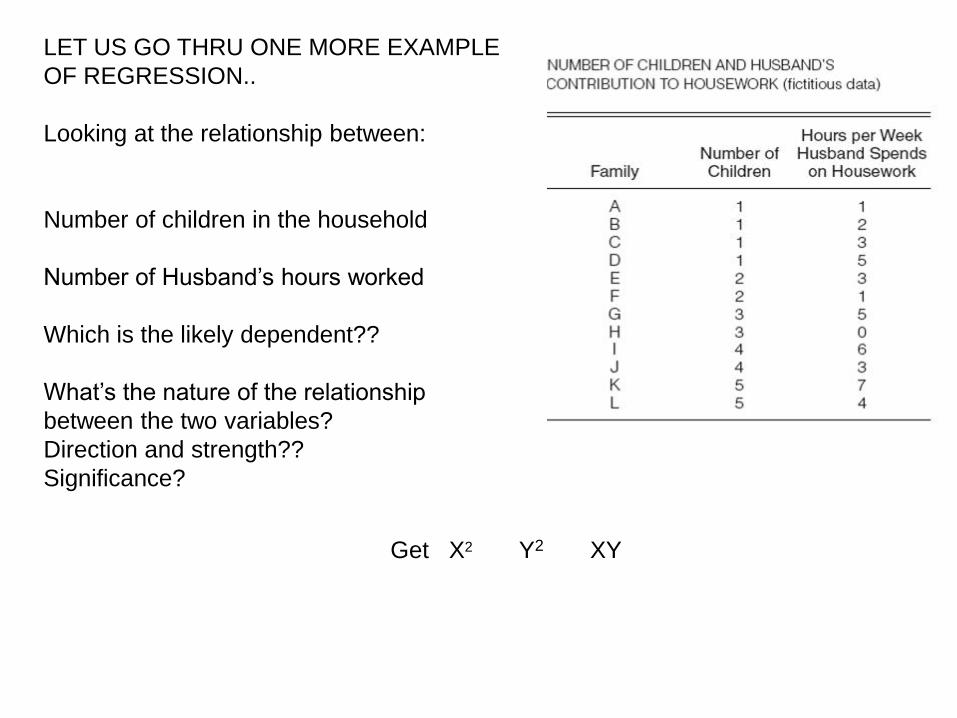
LET US GO THRU ONE MORE EXAMPLE

OF REGRESSION..

Looking at the relationship between:

Number of children in the household

Number of Husband’s hours worked

Which is the likely dependent??

What’s the nature of the relationship

between the two variables?

Direction and strength??

Significance?

Get X2 Y2 XY

15-37

•1. Make computation table, and 2. calculate the means of Y and X

15-38

Regression Analysis (continued)

3. Calculate the slope

15-40

Regression Analysis (continued)

4. Calculate the Y intercept

15-41

• For the relationship between number of children and husband’s housework:– b (slope) = .69– a (Y intercept)= 1.49

• A slope of .69 means that the amount of time a husband contributes to housekeeping chores increases by .69 (less than one hour per week) for every unit increase of 1 in number of children (for each additional child in the family).

• The Y intercept means that the regression line crosses the Y axis at Y = 1.49 (or the value of Y when X is 0).

Interpret

15-42

• Pearson’s r is a measure of association for two interval-ratio variables.

5. Calculate Pearson’s r

])(][)([

))((

2222 YYnXXn

YXXYnr

15-43

• The quantities displayed earlier can again be directly substituted directly into

formula to calculate r for our sample problem

Pearson’s r: An Example

• The quantities displayed earlier can again be directly substituted directly into

formula to calculate r for our sample problem

Pearson’s r: An Example

15-45

• Use the guidelines stated in Table (for gamma) as a guide to interpret the strength of Pearson’s r.– As before, the relationship between the values and the descriptive terms is arbitrary, so

the scale in Table is intended as a general guideline only:

Interpreting Pearson’s r

15-46

• An r of 0.50 indicates a moderate and positive linear relationship between the variables.

– As the number of children in a family increases, the hourly contribution of husbands to housekeeping duties also increases.

– BUT: IS IT SIGNIFICANT????

Interpreting Pearson’s r (continued)

Step 1: Assumptions• Random sample• & additional assumptions…

– The relationship between X and Y is linear. also: interval/ratio level of measurement

6. Testing Statistical Significance

of r

Step 2: Null and Alternate Hypotheses:

• Ho: ρ = 0.0

• H1: ρ ≠ 0.0• (Note that ρ (rho) is the population parameter, while r is the sample

statistic.)

Step 3: Sampling Distribution and Critical Region:

• Sampling Distribution = t-distribution

• Alpha = .05

• DF = n - 2 = 12 - 2 = 10

• tcritical = 2.28 (from the t distribution table)

Step 4. Computing the Test Statistic:

• Use Formula for test statistic:

Step 5. Decision and Interpretation:• Tobtained = 1.826 < tcritical = 2.28

• Can’t Reject Ho. The relationship between the two

variables is not significant!!

83.1)5(.1

2125.

1

222

r

nrtobtained

Always include a brief summary of your results:

• While there initially appeared to be a moderate positive relationship between the two variables, we found that the relationship was non-significant (t=1.826, df=10, α = .05) .