Assignment #5

Chapter 8: 16, 19 Chapter 9: 19 Due this Friday Oct. 30th by 2pm in your TA’s homework box

Assignment #6

Chapter 10: 14, 15 Chapter 11: 14, 18 Due Next Friday Nov. 6th by 2pm in your TA’s homework box

Reading

For Today: Chapter 11 & 12 For Thursday: Chapter 12

First Part of Chapter 11 Review

€

µ = 67.4

€

σ = 3.9

€

µY = µ = 67.4

€

σY =σn

=3.95

=1.7

is normally distributed whenever:

Y is normally distributed or

n is large €

Y

Inference about means

€

Z =Y −µσY

=Y −µσ n

Because is normally distributed, we can convert its distribution to a standard normal distribution:

€

Y

This would give a probability distribution of the difference between a sample mean and the population mean.

But... We don’t know σ . . .

However, we do know s, the standard deviation of our sample. We can use that as an estimate of σ.

€

µ = 67.4

€

σ = 3.9

N In most cases, we don’t know the real population distribution.!

We only have a sample.!

€

SEY =sn

=3.15

=1.4

We use this as an estimate of !

€

σY

€

s = 3.1

€

Y = 67.1

A good approximation to the standard normal is then:

€

t =Y −µSEY

=Y −µs / n

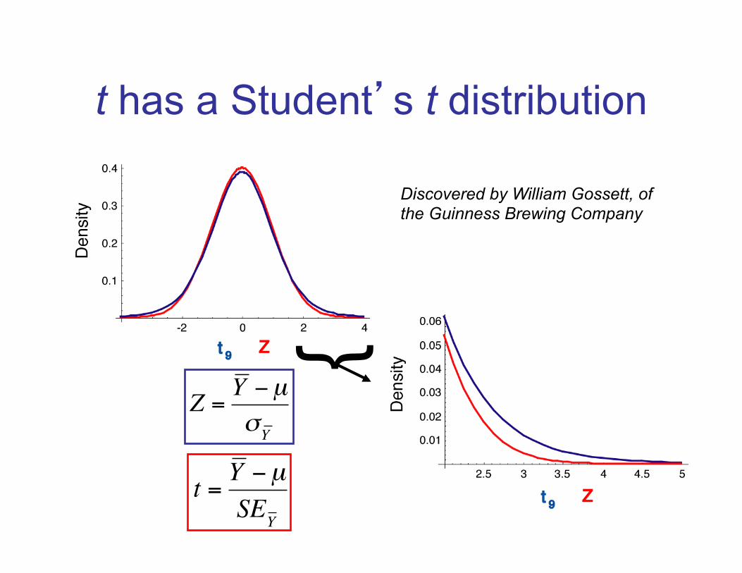
t has a Student’s t distribution

} €

Z =Y −µσY

€

t =Y −µSEY

Discovered by William Gossett, of the Guinness Brewing Company

Degrees of freedom

df = n - 1

We use the t-distribution to calculate an exact confidence

interval of the mean

€

Y ± SEY tα 2( ),df

€

−tα 2( ),df <Y −µSEY

< tα 2( ),df

€

Y − tα 2( ),df SEY < µ < Y + tα 2( ),df SEY

Another way to express this is:

We rearrange the above to generate:

Example Are species ranges shifting towards higher elevations as the world warms? Highest elevation shift (m) over late 1900s and early 2000s was measured for 31 species.

Y = 39.329s = 30.663n = 31

Find the standard error

Y ± SEY tα 2( ),df

SEY =sn=30.66331

= 5.507

Find the critical value of t

df = n−1= 31−1= 30

tα 2( ),df = t0.05 2( ),30= 2.04

Table C: Student's t distribution

Putting it all together...

Y ± SEY tα 2( ),df = 39.329± 5.507 2.04( ) = 39.329±11.234

28.09 < µ < 50.56(95% confidence interval)

99% confidence interval tα 2( ),df = t0.01 2( ),30 = 2.75

Y ± SEY tα 2( ),df = 39.329± 5.507 2.75( ) = 39.329±15.144

24.185< µ < 54.473

One-sample t-test

The one-sample t-test compares the mean of a random sample from a normal population with the population mean proposed in a null hypothesis.

One-sample t-test: Assumptions

•  The variable is normally distributed.

•  The sample is a random sample.

Test statistic for one-sample t-test

€

t =Y − µ 0

s / n

µ0 is the mean value proposed by H0

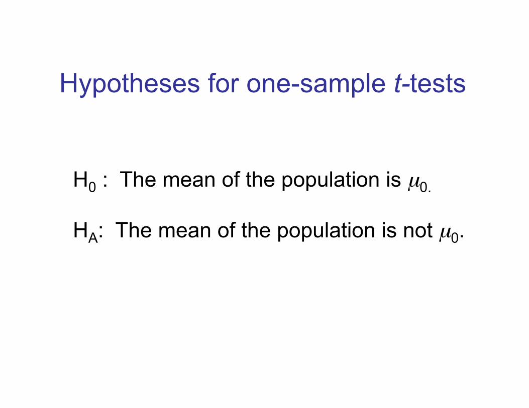
Hypotheses for one-sample t-tests

H0 : The mean of the population is µ0. HA: The mean of the population is not µ0.

Example Are species ranges shifting towards higher elevations as the world warms? Highest elevation shift (m) over late 1900 and early 2000s was measured for 31 species.

Y = 39.329s = 30.663n = 31

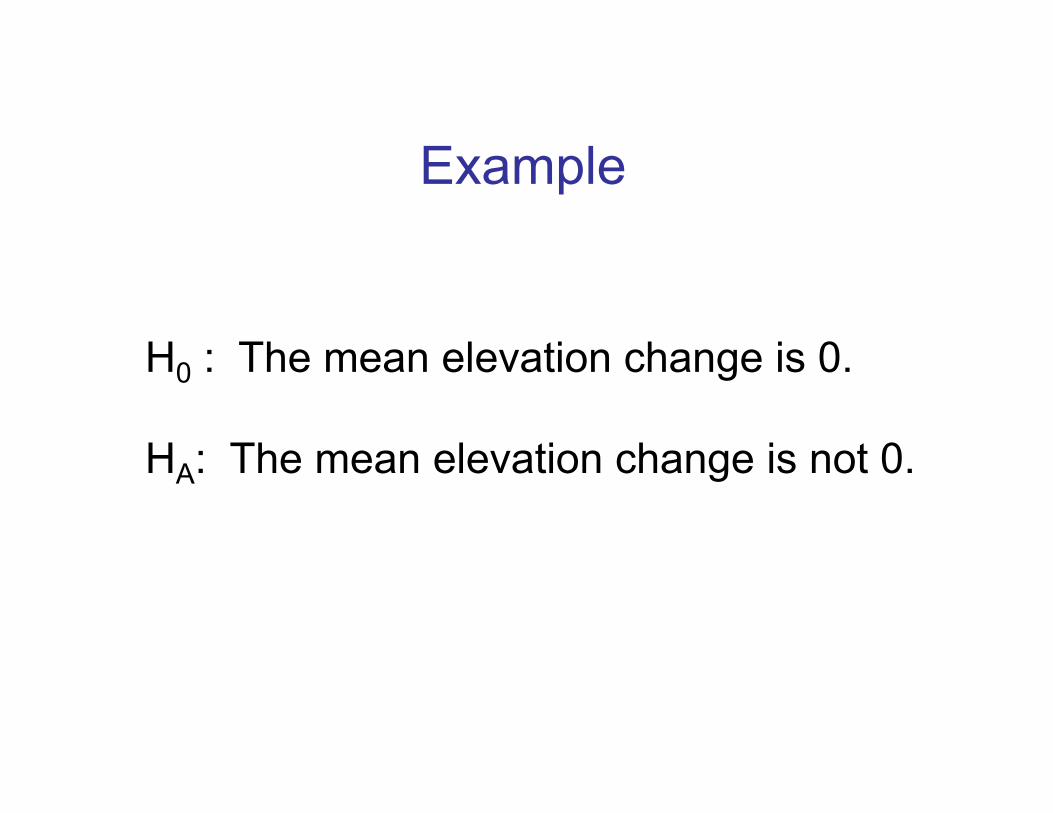
Example

H0 : The mean elevation change is 0. HA: The mean elevation change is not 0.

Example

n = 31Y = 39.329

s / n = 5.507

t = Y −µ0s / n

=39.329− 05.507

= 7.141

Table C: Student's t distribution

Example

t = 7.141

t0.05(2),30 = ±2.04

t is further out in the tail than the critical value, so we reject the null hypothesis. Species have shifted to higher elevations. P<0.0001

t0.0001(2),30 = ±4.48

Inference from a normal population

Chapter 11 Continued

Confidence interval for the variance

€

df s2

χα2

,df

2 ≤σ 2 ≤df s2

χ1−α

2,df

2

χ2

Freq

uenc

y

χ2 1- α/2 χ2 α/2

2.5%

2.5%

α = 0.05

95% confidence interval for a variance

Example: Paradise flying snakes

0.9, 1.4, 1.2, 1.2, 1.3, 2.0, 1.4, 1.6

Undulation rates (in Hz)

€

Y =1.375s = 0.324n = 8

95% confidence interval for the variance of flying snake undulation

rate

€

df s2

χα2

,df

2 ≤σ 2 ≤df s2

χ1−α

2,df

2

df = n - 1 = 7 s2 = (0.324)2 = 0.105

€

χα2,df

2 = χ0.025,72 =16.01

χ1−α2,df

2 = χ0.975,72 =1.69

dfX 0.999 0.995 0.99 0.975 0.95 0.05 0.025 0.01 0.005 0.0011 1.6

E-63.9E-5 0.00016 0.00098 0.00393 3.84 5.02 6.63 7.88 10.83

2 0 0.01 0.02 0.05 0.1 5.99 7.38 9.21 10.6 13.823 0.02 0.07 0.11 0.22 0.35 7.81 9.35 11.34 12.84 16.274 0.09 0.21 0.3 0.48 0.71 9.49 11.14 13.28 14.86 18.475 0.21 0.41 0.55 0.83 1.15 11.07 12.83 15.09 16.75 20.526 0.38 0.68 0.87 1.24 1.64 12.59 14.45 16.81 18.55 22.467 0.6 0.99 1.24 1.69 2.17 14.07 16.01 18.48 20.28 24.328 0.86 1.34 1.65 2.18 2.73 15.51 17.53 20.09 21.95 26.12

Table A

95% confidence interval for the variance of flying snake undulation

rate

€

df s2

χα2

,df

2 ≤σ 2 ≤df s2

χ1−α

2,df

2

7 0.324( )2

16.01≤σ 2 ≤

7 0.324( )2

1.69

0.0459 ≤σ 2 ≤ 0.435

95% confidence interval for the standard deviation of flying snake

undulation rate

€

df s2

χα2

,df

2 ≤σ ≤df s2

χ1−α

2,df

2

0.0459 ≤σ ≤ 0.435

0.21≤σ ≤ 0.66

Comparing two means

Chapter 12

Comparing means

•  Tests with one categorical and one numerical variable

•  Goal: to compare the mean of a numerical variable for different groups.

Paired vs. 2 sample comparisons

Paired comparisons allow us to account for a lot of extraneous variation

2-sample methods are sometimes easier to collect

data for

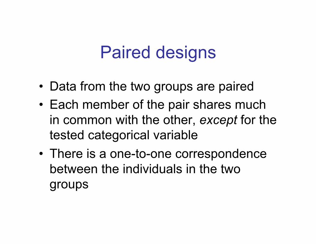
Paired designs

•  Data from the two groups are paired •  Each member of the pair shares much

in common with the other, except for the tested categorical variable

•  There is a one-to-one correspondence between the individuals in the two groups

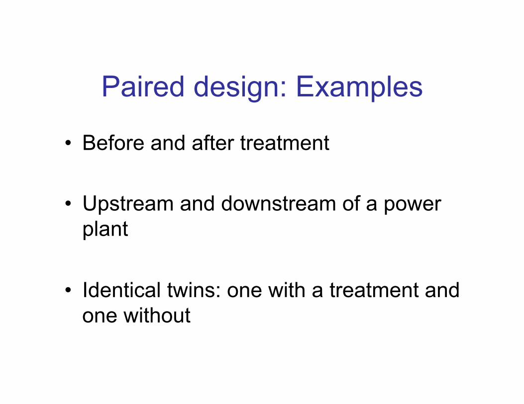
Paired design: Examples

•  Before and after treatment

•  Upstream and downstream of a power plant

•  Identical twins: one with a treatment and one without

Paired comparisons

•  We have many pairs

•  In each pair, there is one member that has one treatment and another who has another treatment

(“Treatment” can mean “group”)

Paired comparisons

•  To compare two groups, we use the mean of the difference between the two members of each pair

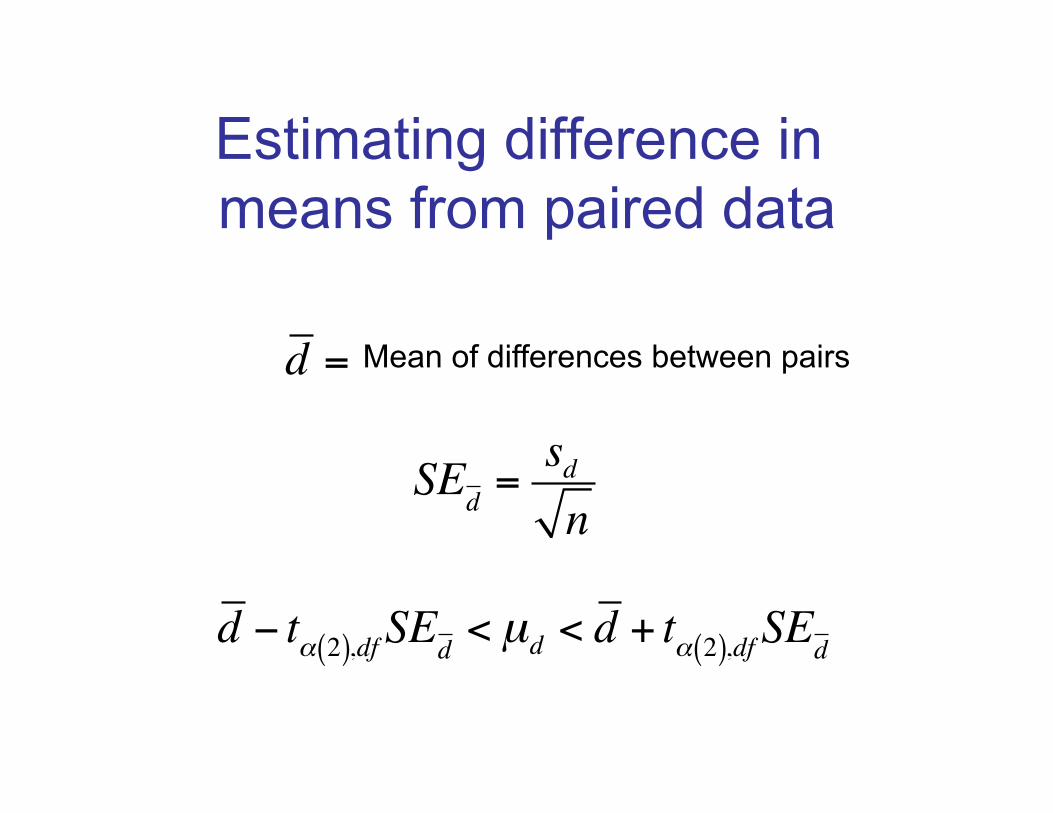
Estimating difference in means from paired data

d − tα 2( ),df SEd < µd < d + tα 2( ),df SEd

SEd =sdn

d = Mean of differences between pairs

Example: National No Smoking Day

•  Data compares injuries at work on National No Smoking Day (in Britain) to the same day the week before

•  Each data point is a year

Data from Waters et al. (1998) Nicotine withdrawal and accident rates. Nature 394: 137.

data

Calculate differences

Estimating difference in means from paired data

25− 2.26(10.2)< µd < 25+ 2.26(10.2)1.948< µd < 48.052

SEd =32.310

=10.2d = 25sd = 32.3n =10 tα 2( ),9 = 2.26

Paired t test

•  Compares the mean of the differences to a value given in the null hypothesis

•  For each pair, calculate the difference. The paired t-test is simply a one-sample t-test on the differences.

Hypotheses

H0: Work related injuries do not change during NoSmoking Days. (µd= 0)

HA: Work related injuries change during No SmokingDays. (µd ≠ 0)

Calculate t using d’s

€

d = 25sd2 =1043.78

n =10

€

t =25− 0

1043.78/10= 2.45

CAUTION!

•  The number of data points in a paired t test is the number of pairs. -- Not the number of individuals

•  Degrees of freedom = Number of pairs - 1

Critical value of t

€

t0.05(2),9 = 2.26t = 2.45 > 2.26

So we can reject the null hypothesis. Stopping smoking increases job-related accidents in the short term.

Assumptions of paired t test

•  Pairs are chosen at random

•  The differences have a normal distribution

It does not assume that the individual

values are normally distributed, only the differences.

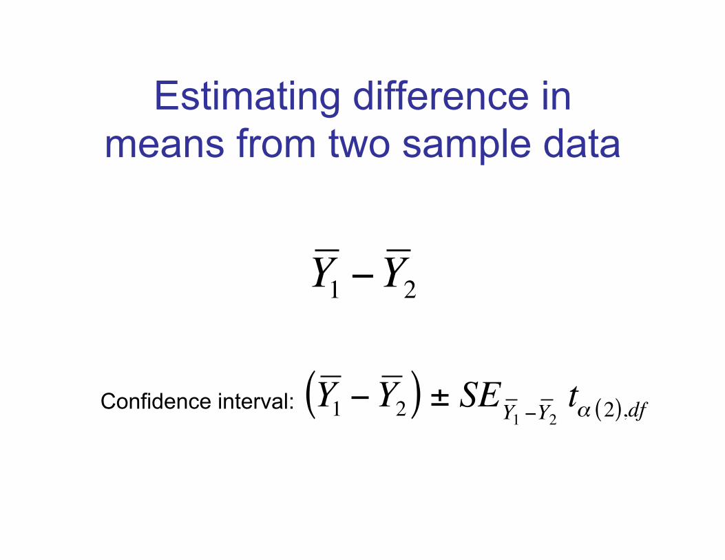
Estimating difference in means from two sample data

€

Y 1 −Y 2

Confidence interval:

€

Y 1 −Y 2( ) ± SEY 1 −Y 2tα 2( ),df

Standard error of difference in means

€

SEY 1 −Y 2=

sp2

n1+

sp2

n2

€

sp2 =

df1s12 + df2s2

2

df1+ df2

df1 = n1 -1; df2 = n2-1

Pooled variance:

Costs of resistance to aphids

2 genotypes of lettuce: Susceptible and Resistant Do these genotypes differ in fitness in the absence of aphids?

Data, summarized

Both distributions are approximately normal.

Susceptible Resistant Mean number of buds

720 582

SD of number of buds

223.6 277.3

Sample size 15 16

Calculating the standard error df1 =15 -1=14; df2 = 16-1=15

€

sp2 =

df1s12 + df2s2

2

df1 + df2=14 223.6( )2 +15 277.3( )2

14 +15= 63909.9

€

SEx 1 −x 2=

sp2

n1+

sp2

n2=

63909.915

+63909.916

= 90.86

Finding t

df = df1 + df2= n1+n2-2

= 15+16-2 =29

€

t0.05 2( ),29 = 2.05

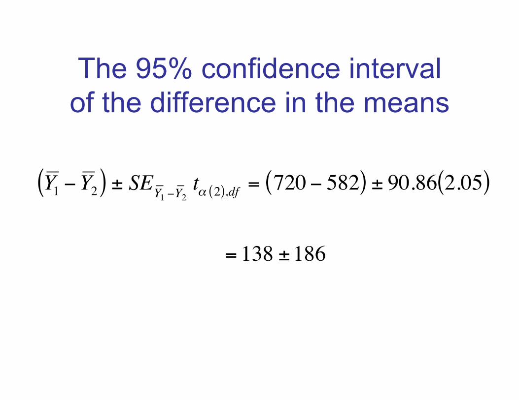
The 95% confidence interval of the difference in the means

€

Y 1 −Y 2( ) ± SEY 1 −Y 2tα 2( ),df = 720 − 582( ) ± 90.86 2.05( )

= 138 ±186

Testing hypotheses about the difference in two means

2-sample t-test

The two sample t-test compares the means of a numerical variable between two populations.

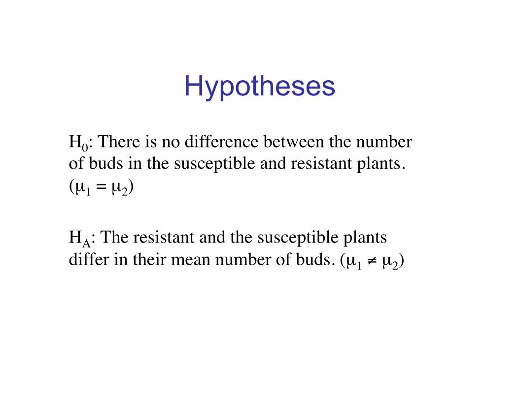
Hypotheses

H0: There is no difference between the number of buds in the susceptible and resistant plants. (µ1 = µ2)

HA: The resistant and the susceptible plants differ in their mean number of buds. (µ1 ≠ µ2)

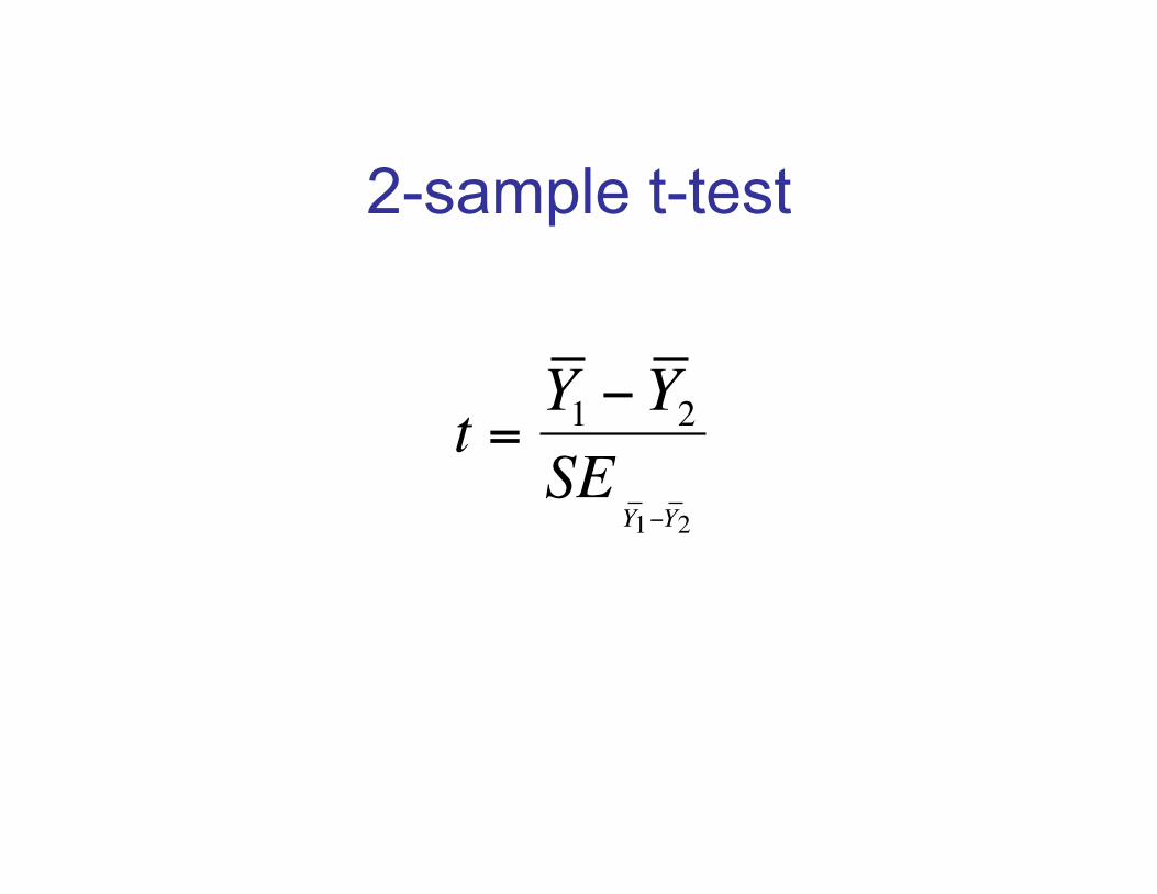
2-sample t-test

€

t =Y 1 −Y 2SE

Y 1−Y 2

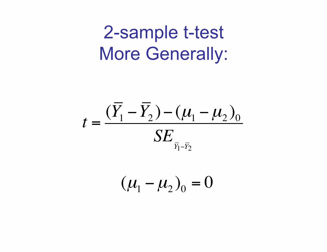
2-sample t-test More Generally:

t = (Y1 −Y2 )− (µ1 −µ2 )0SE

Y1−Y2

(µ1 −µ2 )0 = 0

Calculating t

€

t =Y 1 −Y 2( )SEY 1 −Y 2

=720 − 582( )90.86

= 1.52

Drawing conclusions...

t0.05(2),29=2.05

t <2.05, so we cannot reject the null hypothesis. These data are not sufficient to say that there is a cost of resistance.

Assumptions of two-sample t -tests

•  Both samples are random samples.

•  Both populations have normal distributions

•  The variance of both populations is equal.