System Dynamics Group

Sloan School of Management

Massachusetts Institute of Technology

System Dynamics II, 15.872

Profs. John Sterman and Hazhir Rahmandad

Assignment 2

Understanding Business Fluctuations: The Causes of Oscillations*

Assigned: Wednesday 6 November 2013; Due: Monday18 November 2013

Please do this assignment in a group totaling three people and submit digitally.

Oscillations and cyclic phenomena are among the most common and important dynamic

behaviors. The economy as a whole and many individual industries suffer from chronic

instability in production, demand, employment, and profits, with resulting turnover of top

management. Tempering these industry cycles has proven difficult. This assignment develops

your ability to formulate dynamic models of a business situation and analyze their behavior. You

will build on the model of a firm we developed in class and explore the causes of and cures for

oscillations. The assignment also serves as an introduction to model-based policy analysis.

Case Background: A manufacturing firm, Widgets, Inc., has experienced chronic instability in

its inventory level and production rate.1 Specifically, production and inventory undergo large,

costly variations over time, variations larger than those in incoming orders. Your client,

Widgets, Inc., wants to understand why it has experienced these persistent oscillations, and how

to stabilize operations.

The data show oscillations in inventory and production (while specific data for the Widgets firm

are confidential, the graphs below show large fluctuations in aggregate capacity utilization for the

manufacturing sector of the US economy, and also in overall civilian unemployment).

Originally prepared by John Sterman. Last revision: October 2013.

1 For reasons of confidentiality, the name of the client firm and details of their operations have been disguised.

2

Capacity Utilization, Total Industry (US)

Source: US Federal Reserve

US Civilian Unemployment Rate

Source: US Bureau of Labor Statistics

3

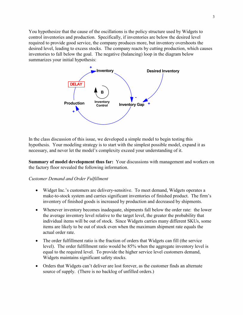
You hypothesize that the cause of the oscillations is the policy structure used by Widgets to

control inventories and production. Specifically, if inventories are below the desired level

required to provide good service, the company produces more, but inventory overshoots the

desired level, leading to excess stocks. The company reacts by cutting production, which causes

inventories to fall below the goal. The negative (balancing) loop in the diagram below

summarizes your initial hypothesis:

Inventory Desired Inventory

Inventory GapProduction +

+

+

-

B

InventoryControl

DELAY

In the class discussion of this issue, we developed a simple model to begin testing this

hypothesis. Your modeling strategy is to start with the simplest possible model, expand it as

necessary, and never let the model’s complexity exceed your understanding of it.

Summary of model development thus far: Your discussions with management and workers on

the factory floor revealed the following information.

Customer Demand and Order Fulfillment

Widget Inc.’s customers are delivery-sensitive. To meet demand, Widgets operates a

make-to-stock system and carries significant inventories of finished product. The firm’s

inventory of finished goods is increased by production and decreased by shipments.

Whenever inventory becomes inadequate, shipments fall below the order rate: the lower

the average inventory level relative to the target level, the greater the probability that

individual items will be out of stock. Since Widgets carries many different SKUs, some

items are likely to be out of stock even when the maximum shipment rate equals the

actual order rate.

The order fulfillment ratio is the fraction of orders that Widgets can fill (the service

level). The order fulfillment ratio would be 85% when the aggregate inventory level is

equal to the required level. To provide the higher service level customers demand,

Widgets maintains significant safety stocks.

Orders that Widgets can’t deliver are lost forever, as the customer finds an alternate

source of supply. (There is no backlog of unfilled orders.)

4

To keep the initial model simple—so that we can learn from it—we assume that

feedbacks to the customer order rate can be omitted for the purpose of this assignment.

Therefore you and the client have agreed to assume that the customer order rate is

exogenous. Later, you may consider adding feedbacks to customer demand (but not for

this assignment). The client is particularly concerned with the response of the firm’s

inventory and production to unanticipated increases in demand (that is, to situations in

which the forecast of demand is erroneous, as is often the case).

Production Scheduling and Inventory Control

The production process involves a significant delay due to the complexity of the

fabrication and assembly process.

The average manufacturing cycle time (the time between the start of the production

process and its completion) is four weeks.

Some items in the product line can be made faster than four weeks, and some take longer.

There is ample plant and equipment to meet demand. Your contact at corporate

headquarters argues that the plant can adjust production starts rapidly to changes in

production schedules.

Desired production (the factory production target) is determined by anticipated

(forecasted) customer orders, modified by a correction to maintain inventory at the

desired level.

The firm continuously compares the desired inventory level to the actual level. They

attempt to correct discrepancies between desired and actual inventory in eight weeks.

Desired inventory is equal to desired inventory coverage multiplied by the forecast of

customer orders. Desired coverage is equal to the minimum order processing time (two

weeks) plus a safety stock of two additional weeks of coverage. The total desired

coverage of four weeks provides enough inventory on average to avoid costly stockouts

without incurring excessive carrying costs.

The desired production start rate depends on the desired rate of production and on the

quantity of work in process (WIP). When WIP is low compared to the level needed to

meet the desired production rate, additional units are started. If WIP is too high relative

to the desired WIP level, production starts are reduced.

The desired level of WIP is the amount required to complete production at the desired

rate given the manufacturing cycle time.

The firm adjusts the level of WIP to the desired level over a two-week period.

5

A. Base Model

The model is called <Widgets> and is available on the CD in the textbook in the Chapter 18

folder, and will a

IMPORTANT: Change the Manufacturing Cycle Time in the Widgets model from 8 to 4

weeks. Use a value of 4 weeks in your base case.

The model is described in detail in chapter 18 (pp. 709-723). Be sure to read this section

carefully so you understand the formulations. In the model customer orders are exogenous

and are determined by a test generator (see Appendix 2 to this assignment). The test generator

makes it easy to challenge the model with a wide variety of patterns for customer orders,

including steps, ramps, cycles, and random noise. Feel free to try your model with any of the

test inputs, particularly noise, but for the purposes of the assignment you only need to use the

step input.

Brevity is a virtue in your write up. Unless specifically requested, do not include complete

sets of output (graphs, tables) for each test and simulation you do. A summary table will

suffice. Construct a table showing the minimum/maximum values of inventory and

production, the amplification ratio, the period of any oscillation, the “settling time” (the time

required for, say, production, to settle within 2% of its equilibrium value), and any other

indicators of performance and stability that are helpful to make your points.

However, as always, you must document and explain the changes you make in the equations

so that an independent third party can replicate your simulations.

To begin your analysis, confirm that your model begins in equilibrium by running the model

without any changes in parameters. Do not hand in the equilibrium run.

Now run the base case of the model with a 20% step input in customer orders in week 5 (set Step

Height = 0.20). Examine the behavior.

The model includes a variety of custom graphs to help you understand its behavior. You may

wish to modify these or create new custom graphs to illustrate the points you wish to make in

your write up. In particular, it is interesting to make a phase plot showing the Production

Start Rate as a function of Inventory.

A1. Briefly explain the model’s base case behavior. Describe in managerial terms (as if you

were presenting your results to the client) what happens after the step increase in

customer orders. Present a minimum of graphs to make your points.

A2.

a. Does the Production Start Rate change by less, the same, or more than the change in

orders? Quantify your response by calculating the amplification ratio (refer to Appendix

1 of this assignment for a discussion of amplification and the amplification ratio).

lso be posted. Copy the model to your hard disk.

6

b. Identify the sources of any amplification.

c. What are the specific structural reasons for the degree of amplification you find? That is,

what parameters and structures control the magnitude of amplification?

A3. Can this model oscillate? Briefly explain why or why not. That is, are there any

circumstances in which this model can generate the reference mode of oscillating

production and inventory?

To answer, you will need to conduct sensitivity tests in which you vary the parameters of

the decision rules and physical structure (see the discussion on sensitivity testing in

chapter 21).

As you make these tests, beware of “DT error”—a situation in which the time period used

to update the stocks is too long relative to the time constants in the system (see Appendix

A in the text on numerical integration).

We are interested in whether the model can endogenously generate an oscillation.

Obviously, if customer orders fluctuate, the production rate will also fluctuate, but that is

not an endogenous oscillation. You want to know if the model will oscillate in response

to a single shock such as an unanticipated step increase in orders.

A4. Can this model oscillate with plausible and realistic parameter values? It is not enough

to generate the behavior of interest in your model. Your model must generate that

behavior for the right reasons. If you find that there are parameter values that cause

oscillation, are these values plausible or realistic? In answering this question consider the

real-life interpretation of the decision processes of the actors in your model. Given the

parameter values needed to generate oscillations, would real firms behave in such a way?

Explain.

B. Extending the Model: Adding the Labor Force

After exploring the behavior of your initial model, you return to the client and argue that the

dynamic hypothesis, as stated, is not sufficient to explain the persistent fluctuations plaguing the

firm. You note that the model currently assumes that the production start rate is equal to the

desired production start rate. This assumption was justified by the statement of a member of the

client team from corporate headquarters that there was ample plant and equipment in the factory,

so that production starts can be altered rapidly to equal the rate called for by the schedule.

Nevertheless, you conclude that the initial model must be revised to include a more realistic

representation of the production start rate.

You visit the plants again to observe how production starts are actually determined, focusing on

whether there are any time delays, and what the sources of delay might be. Your observations

and discussions with plant personnel reveal that, while the firm indeed has ample physical plant

and equipment, labor cannot be hired and trained instantaneously.

7

Changing the workforce is a multi-step process.

First, a target or desired workforce is determined from the production targets developed by

the plant managers. The desired workforce is determined by desired production and average

productivity, which is 20 widgets per worker per week and is quite constant over time.

Next, the desired workforce must be reviewed and authorized by corporate headquarters, a

process that requires an average of four weeks. (During this time analysts examine the latest

cost, inventory, and sales data and try to determine whether the plants’ requests are sensible.

Then their recommendations are forwarded to the relevant management committee, which

deliberates before acting on the plant’s requests.)

There are two inputs to the hiring decision. First, there are replacement hires. Any workers

who quit or retire are replaced immediately. Second, the hiring rate is adjusted above or

below the replacement rate to close any gap between the authorized and actual workforce. Of

course, hiring cannot fall below zero.

Eight weeks are required on average to adjust the actual workforce to the authorized level

through incremental hires. (The delay is due to the time required to create and fill vacancies.)

The firm has a no-layoff policy, and workers stay with the firm an average of 50 weeks (one

year), so any reduction in workforce has to be accomplished through attrition.

Working with your client team, you translate the description of Widgets’ labor policies into the

following policy structure diagrams.

First, the Production Start Rate no longer depends on the Desired Production Start Rate, but

on a new variable, the Normal Production Rate. The Normal Production Rate is the rate of

output achievable by the current Labor Force given Normal Labor Productivity.

8

Discussion with your client suggests that the labor authorization process can be modeled as a

first-order information delay. See Business Dynamics, Ch. 11 for explanation of the different

types of delays. A first order information delay is the same structure used here to model the

demand forecast (expected orders). The Factory Labor Request depends, as described above,

on the Desired Production Start Rate and Normal Labor Productivity. The labor force is

increased by hiring and decreased by the attrition rate. The firm hires to replace attrition and also

adjusts the labor force to the authorized level.

Next, you draw a high-level diagram of the labor supply chain and hiring process.

9

The diagrams that you develop with your clients are not sufficiently detailed for you to begin

writing equations. Expand the diagrams to show explicitly the structure for the delays and

anything else you might need to complete the model. Clearly label the important feedback loops

added. You will need to add a few more variables (both constants and auxiliary variables) to

complete your diagram. Once you have completed the diagram, write the equations for the labor

sector and add them to your model. Wherever possible try to use formulations and structures

analogous to those we have discussed in class! You will not need anything fancy or

complicated.

Do not use built-in functions such as SMOOTH or DELAY. Instead represent the

structures you need explicitly.

Make sure that all units of measure balance and that the model begins in equilibrium (see

section 18.1.5, pp. 716-720, for guidance). Do not hand in the equilibrium run.

B1. Hand in your documented new model (the mdl file), which should include in comments

an explanation of how the equations for labor acquisition capture the verbal description

above.

B2. Before running the model, consider how you think the model will respond to an

unanticipated 20% step increase in customer orders in week 5. Draw by hand the pattern

of behavior you expect for inventories, production starts, and labor. Pay attention to the

10

phase relationships among the variables, that is, the leads and lags of the variables

relative to one another. Hand in your drawing or its picture. (Please do this before

simulating your model. Your grade is not affected by your answer to this question).

B3. Now test the response of the model to a 20% step increase in orders in week 5. This is

your new base run.

a. Hand in graphs showing orders, expected orders, desired production, desired production

starts, production starts, and actual production, all on the same scale.

b. Also hand in a plot of inventory and desired inventory, on the same scale, and a plot of

WIP and Desired WIP, on the same scale.

c. Hand in a plot of Labor and the Factory Labor Request on the same scale.

d. Hand in a graph showing inventory coverage and the order fulfillment ratio.

e. Finally, hand in a phase plot showing Labor vs. Inventory. The phase plot shows

inventory on the x-axis and labor on the y-axis. Use the custom graph feature of Vensim

to create this graph.

B4. Explain the behavior produced by the step increase in shipments. You may find the

explanation emerges naturally as you answer the following questions:

- Why isn’t the system in equilibrium when inventory first equals desired inventory?

- Why isn’t the system in equilibrium when production first equals shipments?

- Why does production overshoot its equilibrium value?

- Why does it undershoot?

Your analysis should proceed step by step, explaining at each juncture in the behavior

what is occurring and why. You should refer to your causal-loop diagram and make use

of your knowledge of stock and flow structures. Also, feel free to plot additional

variables (you may find Vensim’s causal tracing feature valuable); but hand in additional

output only if you refer to it in your explanation. Strive for an explanation that a manager

could understand.

B5.

a. Now that labor is represented in the model, what is the amplification of the production

rate relative to the order rate?

b. Is it larger or smaller than the amplification generated by the model without labor? Why?

c. Identify any new sources of amplification.

C. Policy Analysis: Stabilizing the Firm

11

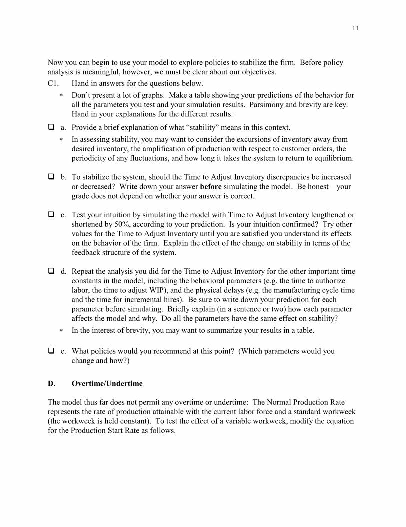
Now you can begin to use your model to explore policies to stabilize the firm. Before policy

analysis is meaningful, however, we must be clear about our objectives.

C1. Hand in answers for the questions below.

Don’t present a lot of graphs. Make a table showing your predictions of the behavior for

all the parameters you test and your simulation results. Parsimony and brevity are key.

Hand in your explanations for the different results.

a. Provide a brief explanation of what “stability” means in this context.

In assessing stability, you may want to consider the excursions of inventory away from

desired inventory, the amplification of production with respect to customer orders, the

periodicity of any fluctuations, and how long it takes the system to return to equilibrium.

b. To stabilize the system, should the Time to Adjust Inventory discrepancies be increased

or decreased? Write down your answer before simulating the model. Be honest—your

grade does not depend on whether your answer is correct.

c. Test your intuition by simulating the model with Time to Adjust Inventory lengthened or

shortened by 50%, according to your prediction. Is your intuition confirmed? Try other

values for the Time to Adjust Inventory until you are satisfied you understand its effects

on the behavior of the firm. Explain the effect of the change on stability in terms of the

feedback structure of the system.

d. Repeat the analysis you did for the Time to Adjust Inventory for the other important time

constants in the model, including the behavioral parameters (e.g. the time to authorize

labor, the time to adjust WIP), and the physical delays (e.g. the manufacturing cycle time

and the time for incremental hires). Be sure to write down your prediction for each

parameter before simulating. Briefly explain (in a sentence or two) how each parameter

affects the model and why. Do all the parameters have the same effect on stability?

In the interest of brevity, you may want to summarize your results in a table.

e. What policies would you recommend at this point? (Which parameters would you

change and how?)

D. Overtime/Undertime

The model thus far does not permit any overtime or undertime: The Normal Production Rate

represents the rate of production attainable with the current labor force and a standard workweek

(the workweek is held constant). To test the effect of a variable workweek, modify the equation

for the Production Start Rate as follows.

12

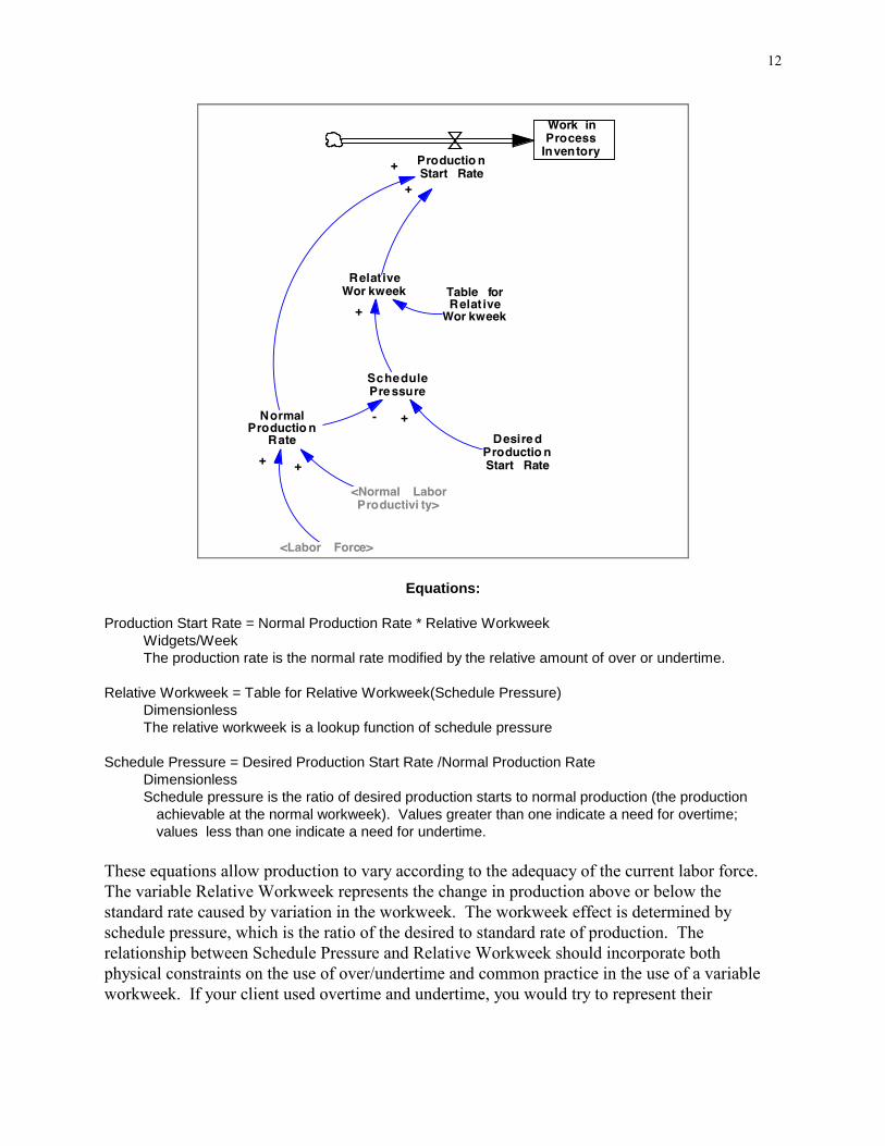
Equations:

Production Start Rate = Normal Production Rate * Relative Workweek

Widgets/Week

The production rate is the normal rate modified by the relative amount of over or undertime.

Relative Workweek = Table for Relative Workweek(Schedule Pressure)

Dimensionless

The relative workweek is a lookup function of schedule pressure

Schedule Pressure = Desired Production Start Rate /Normal Production Rate

Dimensionless

Schedule pressure is the ratio of desired production starts to normal production (the production

achievable at the normal workweek). Values greater than one indicate a need for overtime;

values less than one indicate a need for undertime.

These equations allow production to vary according to the adequacy of the current labor force.

The variable Relative Workweek represents the change in production above or below the

standard rate caused by variation in the workweek. The workweek effect is determined by

schedule pressure, which is the ratio of the desired to standard rate of production. The

relationship between Schedule Pressure and Relative Workweek should incorporate both

physical constraints on the use of over/undertime and common practice in the use of a variable

workweek. If your client used overtime and undertime, you would try to represent their

13

practices. For the base case of the model, set the relative workweek equal to unity for all values

of schedule pressure (no over/under time). The values you use should be:

The input, schedule pressure, runs from 0 to 2 in steps of 0.2. The output, for the base case, is

constant at 1.0 (no over- or undertime). You can try different policies for workweek by changing

the values of the relationship in the simulation dialog box when you run the model.

Don’t change the workweek table function by editing the model. Instead, use the Set button

in the top toolbar, then enter the values for the table by clicking on it in the diagram.

Alternatively, you can change the table values in Synthesim mode by clicking on the table.

Examine the response of the complete model to a 20% step increase in incoming orders, using

the base case parameters and the following overtime policy:

Schedule Pressure Relative Workweek

0.0 1.00

0.2 1.00

0.4 1.00

0.6 1.00

0.8 1.00

1.0 1.00

1.2 1.10

1.4 1.20

1.6 1.25

1.8 1.28

2.0 1.30

14

D1.

a. Explain (in terms a manager would understand) the relationship between Schedule

Pressure and Relative Workweek.

b. What is the meaning of the line Relative Workweek = 1?

c. What is the meaning of the line Relative Workweek = Schedule Pressure?

D2. Explain why the behavior would be stabilized or destabilized by flexible workweeks.

E. Synthesis of Policy Analysis and Recommendations

Now, reflect on what you have learned. Think about the high-leverage points to stabilize the

firm. If you were responsible for reengineering the firm, what policies would you recommend?

You may recommend one of the policies you have tried so far, novel policies you may think of,

or any combination of these. Try to keep your changes realistic (it is not possible to produce or

hire instantly, for example, though you might be able to make substantial cuts in these delays).

Design and simulate your preferred policy.

E1.

a. Give a managerial description of how you believe managers can stabilize their company.

This description differs from a model-based description. For example, managers

probably do not have a parameter called “Inventory Adjustment Time”-–instead they

think in terms of how fast they jump on an inventory problem (words like “panic” or

“relaxed” might be useful). A managerially oriented description moves the focus back to

the real system, and casts your model in its true role as an aid to decision-making, not a

theoretical treatise.

b. After your managerial description, give the model parameters you use to represent this

real-world policy.

E2. Hand in a very brief evaluation of how your policy works in the simulation model. You

might create a table comparing the base case to the your policy run. You might also

include one or two plots comparing the base to the policy run. (Remember to be explicit

about the parameter differences between the two runs—we must be able to replicate your

simulations.)

E3. Hand in the your full, documented model, including overtime and undertime as an mdl

file.

F. What to hand in and how to submit your work

Write up your responses to the questions above in a word (.docx) document. In addition,

you need to submit the various Vensim model (.mdl) files called for in parts B and E.

15

Upload your team’s assig by 5 PM on November 18th

. Submit your

assignment as a single .zip file including your response document and models.

Make sure you include your team-members’ names in the document. Name files with

your team’s name, and for multiple files of the same type, the assignment section, e.g.

“Team21.docx”, “Team21-B.mdl”, all submitted as part of “Team21.zip”.

nment

16

Appendix 1: Amplification

Manufacturing systems tend to amplify changes in incoming orders. “Amplification” is defined

as the ratio of the change in the output of a system to the change in the input, that is A =

Output/Input. (Engineers: amplification is a rough measure of the closed loop gain of the

system.) If A<1, then the system attenuates disturbances in the environment (the output

fluctuates less than the input). Conversely, if A>1, the system amplifies disturbances in the

environment. In the context of the current model, we are interested in the extent to which the

firm’s production management policy amplifies or attenuates changes in incoming orders. That

is, we are interested in the response of production to changes in incoming orders.

To figure the amplification ratio, calculate the maximum change in production as a fraction of

the change in incoming orders. For example, if incoming orders rise from 10,000 to 12,000, then

Input=2,000 units. If production reached a peak of 13,150 units, then Output would be 3,150

units, and amplification A would equal 3,150/2,000=158%.

17

Appendix 2: Test Inputs

System dynamics modeling software provides functions for the most commonly used test inputs:

step, pulse, ramp, sine wave, exponential, and uncorrelated (or “white”) noise, etc. These inputs

are not necessarily intended to correspond to anything that really happened in the past or that will

happen in the future. Rather, the inputs are designed to help you easily explore the dynamics of a

model. With a very simple input, it is easy to see the dynamics generated by the model. More

complicated input patterns, such as actual historical data, make it difficult to isolate the behavior

generated by the model’s structure from the input pattern. Once the dynamics of the structure are

understood, it is usually possible to grasp how the structure will behave with more complicated

inputs such as the actual historical input data.

A useful “Test Input Generator” is provided by the following structure. Note: When using this in

other models, be sure to check the units for time and modify if necessary, along with the default

parameters.

Equations:

Input=

1+STEP(Step Height,Step Time)+

(Pulse Quantity/TIME STEP)*PULSE(Pulse Time,TIME STEP)+

RAMP(Ramp Slope,Ramp Start Time,Ramp End Time)+

STEP(1,Exponential Growth Time)*(EXP(Exponential Growth Rate*Time)-1)+

STEP(1,Sine Start Time)*Sine Amplitude*SIN(2*3.14159*Time/Sine Period)+

STEP(1,Noise Start Time)*RANDOM NORMAL(-4, 4, 0, Noise Standard

Deviation, Noise Seed)

~ Dimensionless

18

~ The test input can be configured to generate a step, pulse, linear

ramp, exponential growth, sine wave, and random variation. The initial value

of the input is 1 and each test input begins at a particular start time. The

magnitudes are expressed as fractions of the initial value.

Step Height=0

~ Dimensionless

~ The height of the step increase in the input.

Step Time=0

~ Day

~ The time at which the step increase in the input occurs.

Pulse Quantity=0

~ Dimensionless*Day

~ The quantity added to the input at the pulse time.

Pulse Time=0

~ Week

~ The time at which the pulse increase in the input occurs.

Ramp Slope=0

~ 1/ Week

~ The slope of the linear ramp in the input.

Ramp Start Time=0

~ Week

~ The time at which the ramp in the input begins.

Ramp End Time=1e+009

~ Week

~ The end time for the ramp input.

Exponential Growth Rate=0

~ 1/ Week

~ The exponential growth rate in the input.

Exponential Growth Time=0

~ Week

~ The time at which the exponential growth in the input begins.

Sine Start Time=0

~ Week

~ The time at which the sine wave fluctuation in the input begins.

Sine Amplitude=0

~ Dimensionless

~ The amplitude of the sine wave in the input.

Sine Period=10

~ Week

~ The period of the sine wave in the input.

Noise Seed=1000

~ Dimensionless

~ Varying the random number seed changes the sequence of realizations

for the random variable.

Noise Standard Deviation=0

~ Dimensionless

~ The standard deviation in the random noise. The random fluctuation

is drawn from a normal distribution with min and max values of +/-

19

4. The user can also specify the random number seed to replicate

simulations. To generate a different random number sequence,

change the random number seed.

Noise Start Time=0

~ Week

~ The time at which the random noise in the input begins.

********************************************************

.Control

********************************************************~

Simulation Control Parameters

FINAL TIME = <user specified>

~ Week

~ The final time for the simulation.

INITIAL TIME = <user specified>

~ Week

~ The initial time for the simulation.

SAVEPER =

TIME STEP

~ Week

~ The frequency with which output is stored.

TIME STEP = <user specified>

~ Week

~ The time step for the simulation.

20

A Note on Random Noise

The random input is useful to simulate unpredictable shocks. The RANDOM_NORMAL

function in Vensim samples from a normal distribution with parameters the user specifies. The

function has the following syntax:

RANDOM_NORMAL (min, max, mean, std dev, seed)

Vensim uses a default random number “seed.” You can specify a different seed by defining a

constant called “Noise Seed” in your model and setting it equal to some value (e.g. Noise Seed =

1000). Vensim generates a single random sequence for any given seed. Let’s say the sequence

is: 0.500, 0.213, 0.678, 0.932, 0.340, 0.015. If there is a single random number function in the

model it will simply yield the random sequence. If there are two or more random functions, the

functions will take turns accessing the sequence. For example, if you have two functions, the

first will yield 0.5, 0.678, 0.34; and the second will yield 0.213, 0.932, 0.015. If you run two

simulations with the same seed, you will get exactly the same sequence of random numbers.

This is important so that you can compare two runs with different policies and be sure the

differences in behavior are due only to the policies and not to different realizations of the random

number generator. When you do want to examine runs with different realizations of the random

process, you need to change the value of the random number seed.

Note also that the use of a function such as RANDOM_NORMAL means a new random number

is selected every time step. Cutting the time step in half would then double the number of

random shocks to which the model is subjected, and increase the highest frequency represented

in the random signal. This is generally not good modeling practice. In realistic models, one must

not only select the standard deviation of any random processes, but also specify its frequency

spectrum (or, equivalently, the autocorrelation function). Failure to do so can lead to spurious

results and make your model overly sensitive to the time step. These issues are discussed in

Appendix B.

A Note on the Pulse Function

The pulse function is used to simulate the effect of instantaneously adding a fixed quantity Q to a

variable. To ensure the entire quantity is added all at once (within a single time step, or DT [delta

time]), the duration of the pulse is set to the smallest interval of time in the model, that is, to the

time step DT. The height of the pulse is then the quantity to be added divided by the time step in

the model, Q/DT. The inflow increases by the height of the pulse and remains at the higher level

for one time step, so that the total quantity added to the accumulation is (Q/DT)*DT = Q units.

MIT OpenCourseWarehttp://ocw.mit.edu 15.872 System Dynamics IIFall 2013 For information about citing these materials or our Terms of Use, visit: http://ocw.mit.edu/terms.