Assignment 1 - cs.anu.edu.au

Assignment 1• Due: 23 Aug 23:59• Grace period until 24 Aug 13:00. No submission

will be accepted after the grace period

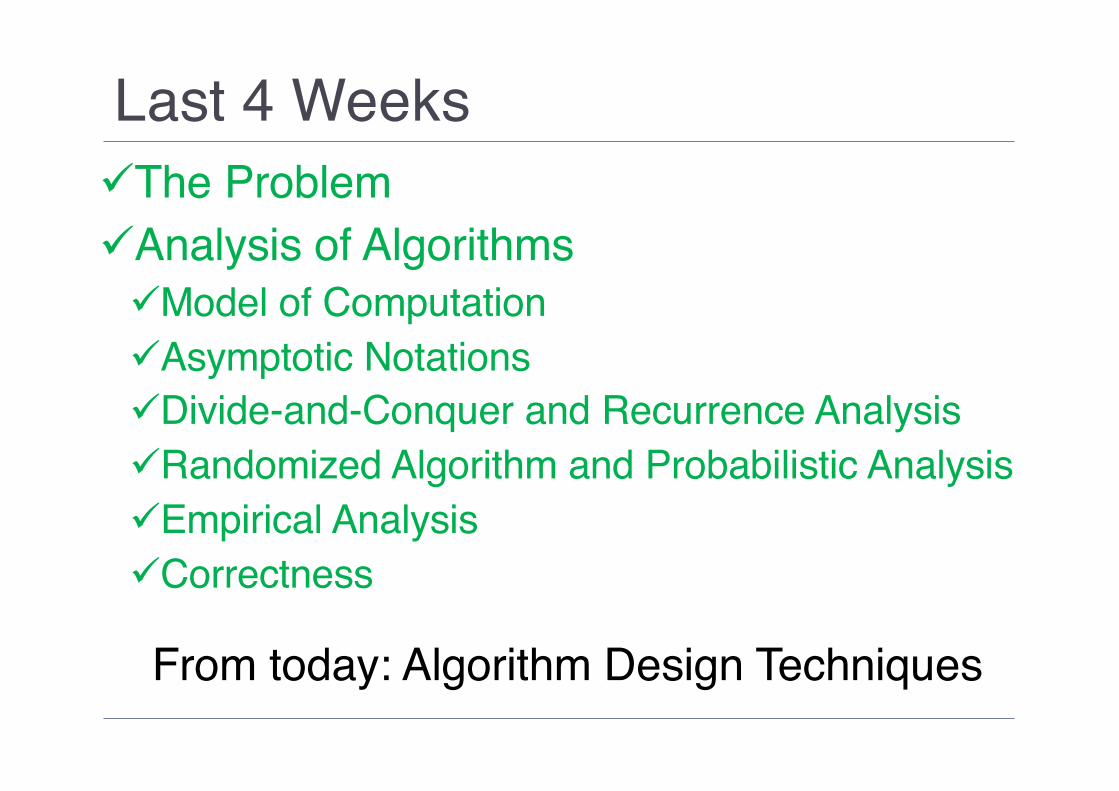
Last 4 WeeksüThe ProblemüAnalysis of AlgorithmsüModel of ComputationüAsymptotic NotationsüDivide-and-Conquer and Recurrence AnalysisüRandomized Algorithm and Probabilistic AnalysisüEmpirical AnalysisüCorrectness

From today: Algorithm Design Techniques

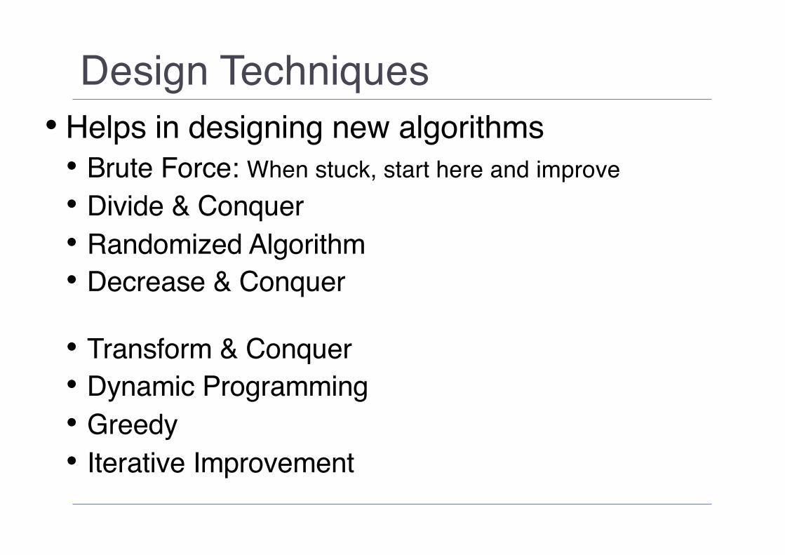
Design Techniques• Helps in designing new algorithms• Brute Force: When stuck, start here and improve• Divide & Conquer: Discussed a bit in recurrence analysis• Randomized Algorithm: Discussed a bit in prob. analysis • Decrease & Conquer: Very similar to divide & conquer,

usually reduced to a smaller sub-problem (e.g., Insertion Sort)• Transform & Conquer• Dynamic Programming• Greedy• Iterative Improvement

Design Techniques• Helps in designing new algorithms• Brute Force: When stuck, start here and improve• Divide & Conquer: Discussed a bit in recurrence analysis• Randomized Algorithm: Discussed a bit in prob. analysis • Decrease & Conquer: Very similar to divide & conquer, but

reduce to 1 smaller sub-problem (e.g., Insertion Sort)• Transform & Conquer• Dynamic Programming• Greedy• Iterative Improvement

Design Techniques• Helps in designing new algorithms• Brute Force: When stuck, start here and improve• Divide & Conquer: Discussed a bit in recurrence analysis• Randomized Algorithm: Discussed a bit in prob. analysis • Decrease & Conquer: Very similar to divide & conquer, but

reduce to 1 smaller sub-problem (e.g., Insertion Sort)• Transform & Conquer: Today + next 1-2 weeks• Dynamic Programming• Greedy• Iterative Improvement

COMP3600/6466 – Algorithms Transform & Conquer 1[Lev sec. 6.1] + [CLRS ch. 8]

+ [CLRS sec. 12.1, 12.2. 12.3]

Hanna Kurniawati

https://cs.anu.edu.au/courses/comp3600/

https://cs.anu.edu.au/courses/comp3600/

Topics• What is Transform & Conquer in Algorithm Design?• Instance Simplification• Common method: Pre-sorting• A bit more about sorting• Representation Change• Supporting Data Structure: • Binary Search Tree • AVL Tree• Red-Black Tree• Heaps

• Examples• Problem Reduction

Today• What is Transform & Conquer in Algorithm Design?• Instance Simplification• Common method: Pre-sorting• A bit more about sorting• Representation Change• Supporting Data Structure: • Binary Search Tree • AVL Tree• Red-Black Tree• Heaps


What is it?• Transform & conquer design technique consists

of 2 stages:• Transform the problem• Solve the transformed problem• Of course, the goal is that the transformation

should make solving easier. • There’s 3 types of transformations:• Instance simplification• Representation change• Problem reduction

TodayüWhat is Transform & Conquer in Algorithm Design?• Instance Simplification• Common method: Pre-sorting• A bit more about sorting• Representation Change• Supporting Data Structure: • Binary Search Tree • AVL Tree• Red-Black Tree• Heaps


What is Instance Simplification?• Transform a problem to a simpler version of the

same problem• Commonly used method: Pre-sorting• Finding solutions in a list of sorted numbers are

usually easier than in an unsorted one• This is why sorting is considered an important problem• Examples of how it’s used: Tutorial-1 Q4 (finding a

particular value), check if all elements in an array are unique (i.e., the array contains no duplicates)

Example: Check for uniqueness• Input: A[0, …, n]• Output: True if all numbers in A appear only once

in A, False otherwise• Brute force: Compare every pair• Worst case #comparisons (and hence, run-time): Θ(𝑛$)• Transform & conquer:

1. Sort: Some algorithms have run-time 𝑂(𝑛 log 𝑛)2. Check whether two consecutive elements are the

same or not: Θ(𝑛)

TodayüWhat is Transform & Conquer in Algorithm Design?• Instance SimplificationüCommon method: Pre-sorting• A bit more about sorting• Representation Change• Supporting Data Structure: • Binary Search Tree • AVL Tree• Red-Black Tree• Heaps


A bit more about Sorting• So far, we’ve seen 4 different sorting methods• Insertion sort, Bubble sort, Merge sort,

Randomized Quick sort• All of the above are comparison-based• Meaning: The sorted order is based only on

comparisons between the input elements • Comparison-based sort requires Ω(𝑛 log 𝑛)

comparisons. Hence, their run-time complexity must be Ω(𝑛 log 𝑛) too. Therefore, those methods whose run-time complexity is Θ(𝑛 log 𝑛) is (close to) optimal

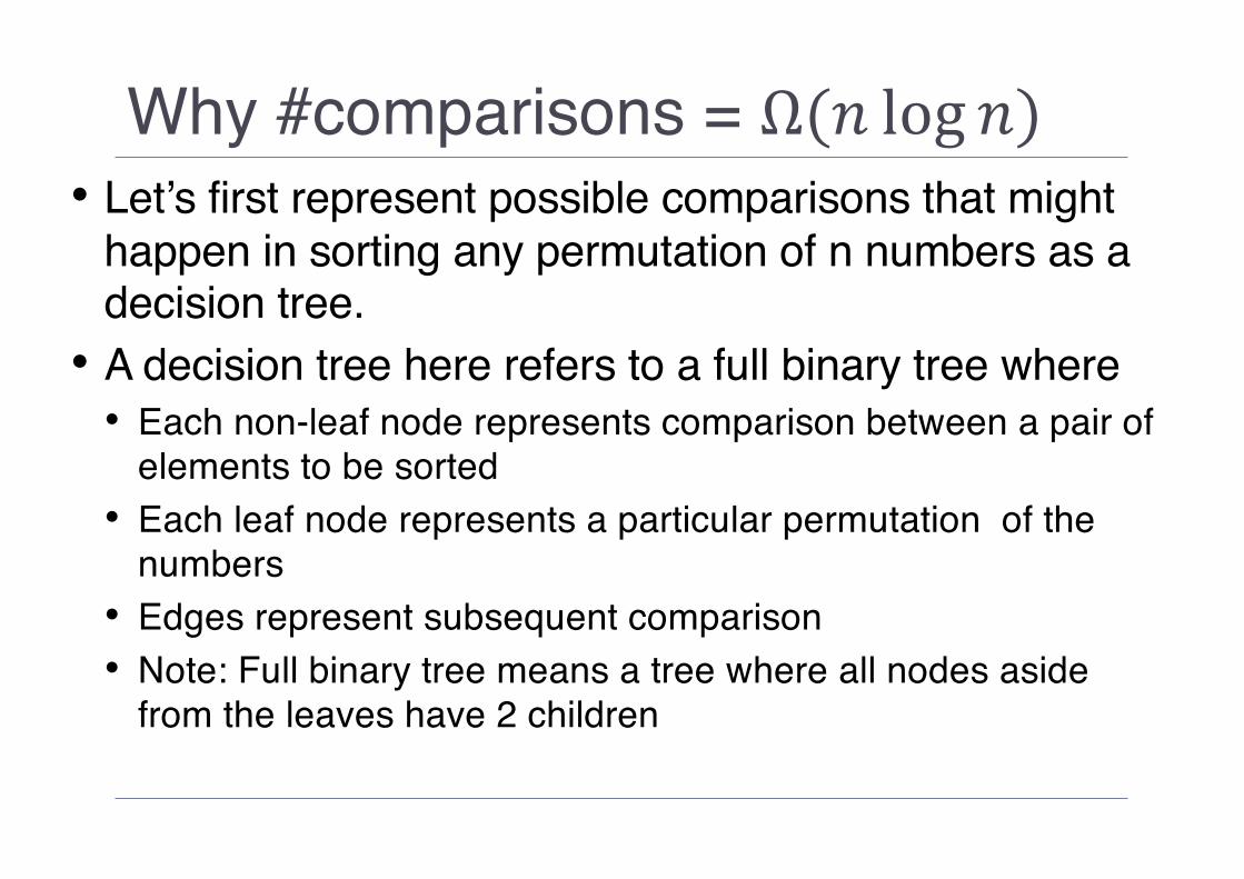
Why #comparisons = Ω(𝑛 log 𝑛)• Let’s first represent possible comparisons that might

happen in sorting any permutation of n numbers as a decision tree. • A decision tree here refers to a full binary tree where• Each non-leaf node represents comparison between a pair of

elements to be sorted• Each leaf node represents a particular permutation of the

numbers• Edges represent subsequent comparison• Note: Full binary tree means a tree where all nodes aside

from the leaves have 2 children

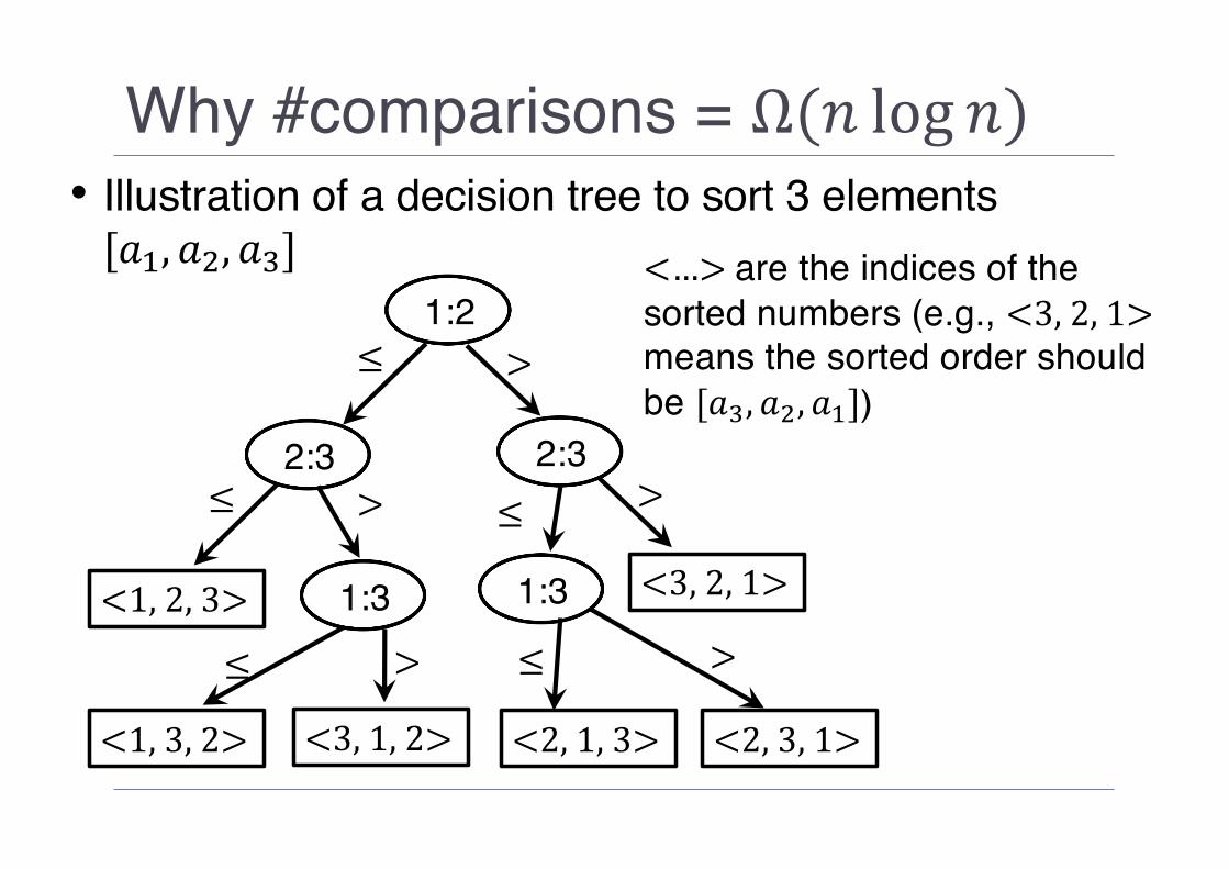
Why #comparisons = Ω(𝑛 log 𝑛)• Illustration of a decision tree to sort 3 elements [𝑎-, 𝑎$, 𝑎/]

<2,1,3>

1:2

2:3 2:3

≤ >

≤ > ≤ >

1:3

≤ >

<1,2,3> <3,2,1>1:3

≤ >

<1,3,2> <3,1,2> <2,3,1>

<…>are the indices of the sorted numbers (e.g., <3,2,1>means the sorted order should be [𝑎/, 𝑎$, 𝑎-])

Why #comparisons = Ω(𝑛 log 𝑛)• The decision tree that represents the problem of

sorting n elements would have n! leaf nodes• A path from the root to a leaf node of the tree

represents comparison for sorting a particular permutation of n numbers. • In the worst case, the number of comparisons would

be the same as the height of the tree.• Since there’s n! leaf nodes in the tree, the height of the

tree is log 𝑛! = ∑<=-> log 𝑖 = 𝑛 log 𝑛• Therefore, any comparison-based sorting requires Ω(𝑛 log 𝑛) in the worst case

Can we sort without comparing?• Yes, we can!• In fact, run-time complexity can be better

without comparison• Examples: • Counting Sort, Radix Sort, Bucket Sort

Non-comparison based Sorting: Counting Sort • Assumption: Sorting integers of a small range• If the #elements to be sorted (i.e., n) is large but

the range is small, there must be many elements with the same values• Counting sort uses this observation to sort the

elements by counting elements of the same values• The result of counting is used to get a rough idea of the

position of each element once the numbers are sorted

Non-comparison based Sorting: Counting Sort

Non-comparison based Sorting: Counting Sort: Illustration

• A

• Set C as #elements in A whose values are = C’s index

• Set C as #elements in A whose values are ≤ C’ index

Index 1 2 3 4 5 6Value 3 4 0 2 0 2

Index 0 1 2 3 4Value 2 0 2 1 1

Index 0 1 2 3 4Value 2 2 4 5 6

Non-comparison based Sorting: Counting Sort: Illustration

• Output B by assigning values of A at index based on values of C & update C• B:

• C:

• Step-2• B:

• C:

Index 1 2 3 4 5 6Value 2

Index 0 1 2 3 4Value 2 2 3 5 6

Index 1 2 3 4 5 6Value 0 2

Index 0 1 2 3 4Value 1 2 3 5 6

Non-comparison based Sorting: Counting Sort

Non-comparison based Sorting: Counting Sort: Running-time• The running-time complexity: Θ(𝑛 + 𝑘) where 𝑛 is the

input size and the input ranges from 0 to 𝑘• Since counting sort is often used for problems where 𝑘 is

much smaller than 𝑛, the complexity is often stated as Θ(𝑛)• However, if counting sort is applied to problems where the

range of numbers (i.e., (𝑘 − 0)) is much larger than 𝑛, then the complexity is Θ(𝑘). And if both 𝑛 and 𝑘 are similar, then the complexity should be stated as Θ(𝑛 + 𝑘)

• Note that elements with the same values appear in the output array in the same order as they appear in the input array. This property is called stable and is quite useful (e.g., in Radix Sort).

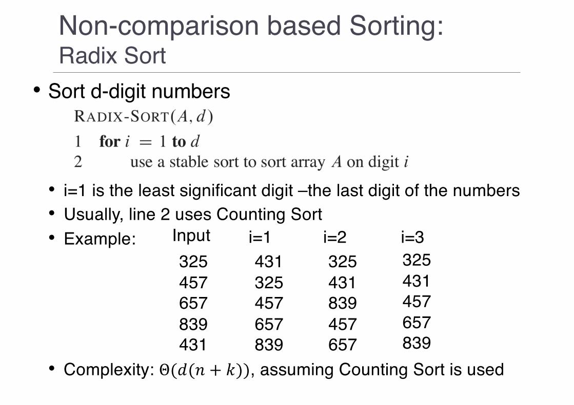
Non-comparison based Sorting: Radix Sort

• Sort d-digit numbers

• i=1 is the least significant digit –the last digit of the numbers • Usually, line 2 uses Counting Sort• Example:

• Complexity: Θ(𝑑(𝑛 + 𝑘)), assuming Counting Sort is used

325457657839431

Input431325457657839

i=1325431839457657

i=2325431457657839

i=3

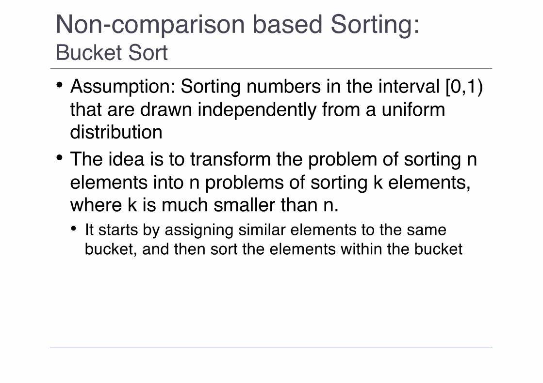
Non-comparison based Sorting: Bucket Sort • Assumption: Sorting numbers in the interval [0,1)

that are drawn independently from a uniform distribution • The idea is to transform the problem of sorting n

elements into n problems of sorting k elements, where k is much smaller than n. • It starts by assigning similar elements to the same

bucket, and then sort the elements within the bucket

Non-comparison based Sorting: Bucket Sort

Non-comparison based Sorting: Bucket Sort: Illustration

0.780.170.390.260.720.940.210.120.230.68

123456789

10

A0123456789

B

0.78

0.17

0.390.26

0.72

Non-comparison based Sorting: Bucket Sort: Illustration

Non-comparison based Sorting: Bucket Sort: Running-time• 𝑇 𝑛 = Θ 𝑛 + ∑<=F>G-𝑂(𝑛<$)

• Average case:𝐸[𝑇 𝑛 ] = 𝐸[Θ 𝑛 + ∑<=F>G-𝑂 𝑛<$ ]

Using linearity of expectation, we have𝐸[𝑇 𝑛 ] = 𝐸[Θ 𝑛 ] + ∑<=F>G-𝐸[𝑂 𝑛<$ ]𝐸[𝑇 𝑛 ] = Θ 𝑛 + ∑<=F>G-𝑂 𝐸[𝑛<

$]

Cost of Insertion Sort in bucket-𝑖

Non-comparison based Sorting: Bucket Sort: Running-time• Now, we need to compute 𝐸[𝑛<$ ] where 𝑛< is the

expected number of elements in bucket- 𝑖• Use Indicator Random Variable

• 𝑋<,J = 𝐼 𝐴 𝑗 𝑖𝑛 𝑏𝑢𝑐𝑘𝑒𝑡 𝑖 = S1 𝐴 𝑗 𝑖𝑛 𝑏𝑢𝑐𝑘𝑒𝑡 𝑖0 𝑂𝑡ℎ𝑒𝑟𝑤𝑖𝑠𝑒

• Since the input are independent and uniformly distributed samples, 𝑃(𝑋<,J = 1) = -

>

Non-comparison based Sorting: Bucket Sort: Running-time• Now, we can compute: 𝐸[𝑛<

$ ] = 𝐸 ∑J=-> 𝑋<,J$

= 𝐸 ∑J=-> ∑Y=-> 𝑋<,J𝑋<,Y= 𝐸 ∑J=-> 𝑋<,J$ + ∑J=-> ∑-ZYZ>,Y[J 𝑋<,J𝑋<,Y= ∑J=-> 𝐸[𝑋<,J$ ] + ∑J=-> ∑-ZYZ>,Y[J 𝐸[𝑋<,J𝑋<,Y]

𝐸 𝑋<,J$ = 1$. ->+ 0$ 1 − -

>= -

>

𝐸 𝑋<,J𝑋<,Y = 𝐸 𝑋<,J 𝐸 𝑋<,J = ->->= -

>]

Non-comparison based Sorting: Bucket Sort: Running-time• Now, we can plug the expected values back to

𝐸[𝑛<$ ] = ∑J=-> 𝐸[𝑋<,J$ ] + ∑J=-> ∑-ZYZ>,Y[J 𝐸[𝑋<,J𝑋<,Y]

= ∑J=-> ->+ ∑J=-> ∑-ZYZ>,Y[J

->]

= 𝑛 ->+ 𝑛 𝑛 − 1 -

>]= 1 + (>G-)

>= 2 − -

>

• Returning to 𝑇 𝑛 :𝑇 𝑛 = Θ 𝑛 +∑<=F>G-𝑂(𝑛<$)

= Θ 𝑛 + 𝑛.𝑂 2 − ->

= Θ 𝑛

Notes-1• Comparison-based methods can be used to sort any

type of data, as long as there’s a comparison function• Its running-time complexity is asymptotically lower bounded

by 𝑛 log 𝑛 --that is, Ω(𝑛 log 𝑛), where n is the input size• Non comparison-based can run in linear time. But, it

assumes the data to be sorted is of a certain type.• Tips: More efficient algorithms can be developed by

focusing on a sub-class of a problem sub-class (in the sorting case, a particular type of input).

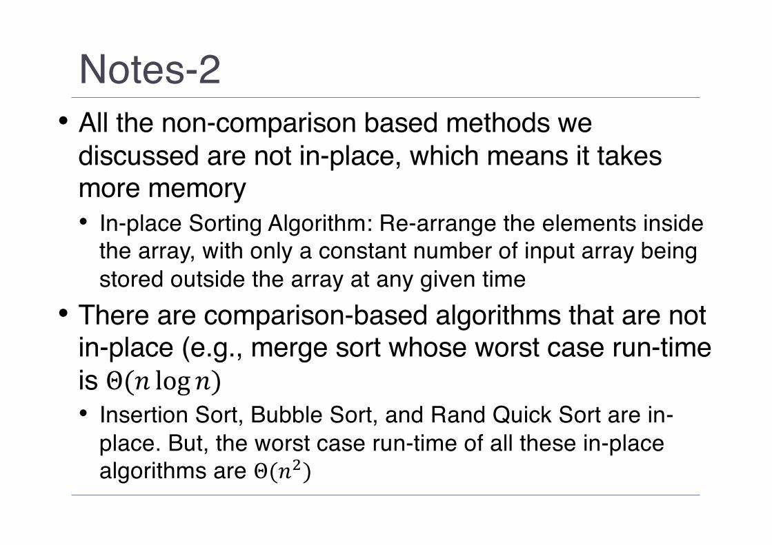
Notes-2• All the non-comparison based methods we

discussed are not in-place, which means it takes more memory• In-place Sorting Algorithm: Re-arrange the elements inside

the array, with only a constant number of input array being stored outside the array at any given time

• There are comparison-based algorithms that are not in-place (e.g., merge sort whose worst case run-time is Θ(𝑛 log 𝑛)• Insertion Sort, Bubble Sort, and Rand Quick Sort are in-

place. But, the worst case run-time of all these in-place algorithms are Θ(𝑛$)

Notes-2• Tips: Pay attention to Speed vs Memory tradeoff• Usually we can make an algorithm faster by using more

memory and vice versa• Tips: Randomization sometimes help speed-up

while keeping memory requirement low• Example: Rand Quick Sort allows average case running-

time to be Θ(𝑛 log 𝑛) and in practice tend to be close to this average case rather than the worst case Θ(𝑛$)

TodayüWhat is Transform & Conquer in Algorithm Design?üInstance SimplificationüCommon method: Pre-sortingüA bit more about sorting• Representation Change• Supporting Data Structure: • Binary Search Tree • AVL Tree• Red-Black Tree• Heaps


What is Representation Change?• Recall that algorithms transform input to output. This

usually means the algorithm will perform certain operations on the input data, so as to transform them into the desired output• The way these data are represented in the algorithm

could often influence the efficiency of the algorithm• Representation Change technique transforms the way

the data are being represented, so that solving becomes more efficient• This is particularly useful when the data is dynamic, i.e., the

input might change (the input size might increase, decrease, or the content changes) during run-time

Abstract Data Structures• The way these data are represented are often called

Abstract Data Structure• Abstract Data Structures can be thought of as a

mathematical model for data representation. An Abstract Data Structure consists of two components:• A container that holds the data • A set of operations on the data. These operations are

defined based on their behavior, rather than their exact implementation

What is Binary Search Tree (BST)?• An abstract data structure that represents the data as

a binary tree with the following property:• Each node in the tree contains the data itself, as key +

satellite data, and pointers to its left child, right child, and parent node, usually denoted as left, right, p• Key: Data used for BST operations. In BST, all keys are

distinct• Satellite data: Data carried around but not used in the

implementation• The root node is the only node with p = NIL

• Suppose 𝑥 is a node of the BST. If 𝑦 is the left sub-tree of 𝑥then, 𝑦. 𝑘𝑒𝑦 ≤ 𝑥. 𝑘𝑒𝑦. If 𝑦 is the right sub-tree of 𝑥 then, 𝑦. 𝑘𝑒𝑦 ≥ 𝑥. 𝑘𝑒𝑦.

• Provide operations Search, Min, Max, Successor, Predecessor, Insert, Delete in 𝑂 ℎ time, where ℎ is the height of the tree

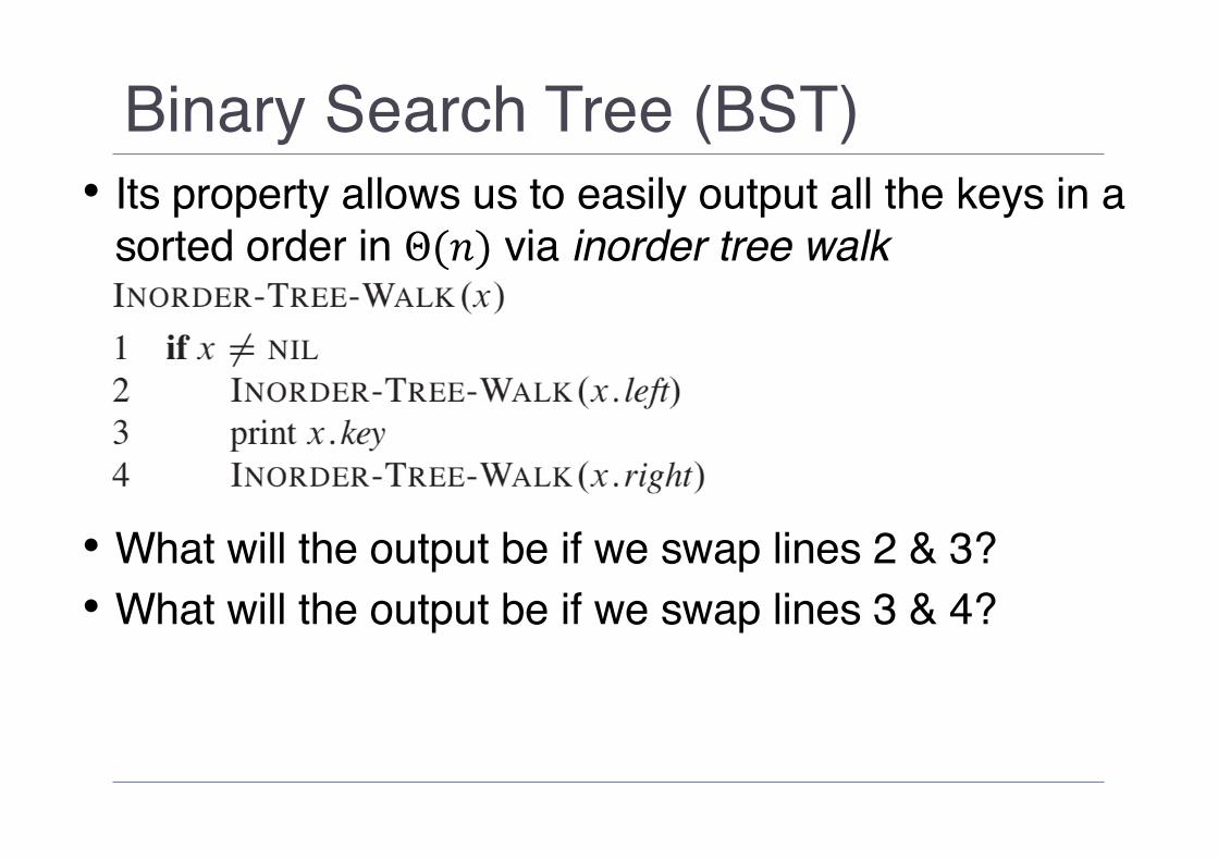
Binary Search Tree (BST)• Its property allows us to easily output all the keys in a

sorted order in Θ(𝑛) via inorder tree walk

• What will the output be if we swap lines 2 & 3?• What will the output be if we swap lines 3 & 4?

Binary Search Tree: Search Operation• To search for a key whose value is 𝑘:

Binary Search Tree : Min & Max•Where’s the Min in a BST?•Where’s the Max in a BST?

Binary Search Tree: Successor & Predecessor

• Successor of a node 𝑥 is the node with the smallest key greater than 𝑥. 𝑘𝑒𝑦 –that is, the node visited right after 𝑥 in inorder tree walk• If 𝑥 has a non-empty right sub-tree, its successor is the

minimum of its right sub-tree• Otherwise, 𝑥’s successor is the lowest ancestor of 𝑥 whose

left child is also an ancestor of 𝑥• Predecessor of a node 𝑥 is the node with the largest

key smaller than 𝑥. 𝑘𝑒𝑦 –that is, the node visited right before 𝑥 in inorder tree walk• If 𝑥 has a non-empty left sub-tree, its predecessor is the

maximum of its left sub-tree• Otherwise, 𝑥’s successor is the lowest ancestor of 𝑥 whose

right child is also an ancestor of 𝑥

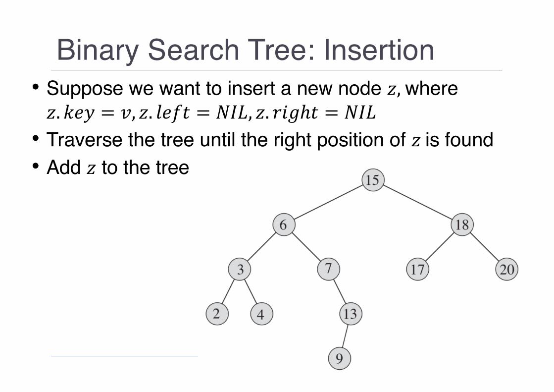
Binary Search Tree: Insertion• Suppose we want to insert a new node 𝑧,where 𝑧. 𝑘𝑒𝑦 = 𝑣, 𝑧. 𝑙𝑒𝑓𝑡 = 𝑁𝐼𝐿, 𝑧. 𝑟𝑖𝑔ℎ𝑡 = 𝑁𝐼𝐿• Traverse the tree until the right position of 𝑧 is found• Add 𝑧 to the tree

Binary Search Tree: Insertion

Binary Search Tree: Deletion• Suppose we want to delete 𝑧. There’s 3 cases:• When 𝑧 has no children: Remove 𝑧 and modify its parent to

replace 𝑧 with NIL• When 𝑧 has only 1 child: Elevate the child to take 𝑧’s position

in the tree by modify its parent to replace 𝑧 with 𝑧’s child• When 𝑧 has 2 children, consider its successor 𝑦 (since 𝑧 has

2 children, 𝑦 must be in its right subtree) : • If 𝑦 is 𝑧’s right child, replace 𝑧 with 𝑦• If 𝑦 is not 𝑧’s right child, first replace 𝑦 by its right child and

then replace 𝑧 with 𝑦

Some Notes on Run-Time Complexity• Aside from the tree walk, all operations

discussed before have run-time complexity of Θ(ℎ) where ℎ is the tree’s depth• The question is, what is ℎ with respect to

the input size 𝑛? If the tree is a full binary tree, ℎ = Θ log 𝑛 . But if we’re not careful, we have ℎ = 𝑛.• How to ensure that ℎ is as close to Θ log 𝑛

as possible? Tree rebalancing

TodayüWhat is Transform & Conquer in Algorithm Design?üInstance SimplificationüCommon method: Pre-sortingüA bit more about sorting• Representation Change• Supporting Data Structure:

üBinary Search Tree • AVL Tree• Red-Black Tree• Heaps


Next Week: AVL Tree + Red-black Tree + Heaps

Assignment 1 - cs.anu.edu.au

Documents

Transcript of Assignment 1 - cs.anu.edu.au