Assessment of the Possibility to Measure Deformations of...

GEOMATICS AND ENVIRONMENTAL ENGINEERING • Volume 10 • Number 2 • 2016

http://dx.doi.org/10.7494/geom.2016.10.2.15

15

Paweł Ćwiąkała*, Paweł Wiącek*

Assessment of the Possibility to Measure Deformations of Rock Walls

Using Terrestrial Laser Scanning**

1. Introduction

Unexpected rockfalls and rock displacements belong to most signifi cant dan-gers related to slope engineering. It may cause not only serious changes in the en-vironment but also, and most of all, danger for infrastructure and can even lead to fatal accidents. Therefore, ensuring security in both open-pit mining and on the rocky slopes in the area of road cuts requires instant monitoring of the stability and displacements of slopes and determining the dynamics of emerging changes [1–3]. Data concerning rock mechanics provided by the measurements enable undertaking proper actions in order to predict the development of movement and start preven-tive and protective works [4]. Currently, the most often used methods of measur-ing rock geometry are direct methods (total station). On the other hand, in order to defi ne additional slope parameters, specialized measuring systems (extensometer, inclinometer) are used. Using classic surveying instruments imposes considerable limitations caused by the necessity to generalization and interpolation of obtained measurement results. The same applies to slope stress and strain measurements. Dynamic development of surveying technologies including Terrestrial Laser Scan-ning (TLS) allows for fast retrieval of measurement data. The additional advantage of TLS is its ability to quickly obtain data of very high resolution and accuracy with-out direct contact with the examined object. Thus, it allows for the carrying out mea-surements for the whole object without the need for generalization. It off ers new possibilities for analysis and interpretation of obtained results [5, 6].

This paper presents the possibilities of using TLS method for marking displace-ments and volume of rock cavities formed as a result of natural and anthropogenic weathering. Discussed works are supported by exemplary measurements conduct-ed in the area of abandoned limestone quarry “Zakrzówek” in Cracow.

* AGH University of Science and Technology, Faculty of Mining Surveying and Environmental Engi-neering, Krakow, Poland

** The paper was prepared within the scope of the Dean Project of the Faculty of Mining Surveying and Environmental Engineering (AGH University of Science and Technology) no. 15.11.150.388.

16 P. Ćwiąkała, P. Wiącek

2. The Object of the Study

Three rock walls were selected for this study. The fi rst of them was recognized as a laboratory case due to its solid structure and low susceptibility to weathering. Its geological structure is very similar to the others. Thus, it was used to determine the accuracy and reproducibility of performed studies. The other two objects are subject to natural weathering (freeze-thaw and biogeochemical weathering) and in-tensive anthropogenic weathering.

Due to numerous climbing lines situated on the rock walls, periodic cleaning of the fragments of loosely-connected rocks has to be held in order to ensure security of the climbers. Such works have been completed between fi rst and second measure-ment series.

3. Field Measurements

The fi rst step of fi eld works was to create and measure the control network. Its main task is to preserve the maximum measurement reproducibility between suc-cessive measuring sessions. Network points were mounted in a way that allows for the minimization of point cloud registration error. Four permanent ground control points, equally distributed on measuring objects, were fi xed for this purpose. Fifteen centimeter long threaded studs, glued inside the holes drilled in the solid rock frag-ments, were used for mounting. This way, forced centering points for circular planar target Leica HDS 6 were established.

During the fi rst measuring session (4 February 2014) network points were mea-sured by refl ectorless total station Leica TCRA 1102plus and additionally a static GNSS measurement with two Leica GPS1200 receivers was performed for georef-erencing in a state system. Additionally, in order to control the stability of control points, tacheometry measurements of the network geometry were carried out during each measurement session.

A key step of fi eld works was related to TLS measurements carried out in four measuring sessions (4 February 2014, 14 March 2014, 7 November 2014, 15 March 2015). TLS measurement was performed by time-of-fl ight scanner Leica ScanSta-tion C10. Scans of particular objects were taken from one station with the resolution of 5 × 5 mm on the maximum distance to the measured object, however, distances for particular objects ranged between 20–50 m. Tests regarding diff erent distances between the scanner and the object were not performed. It was considered that the previously mentioned range is suffi cient for examining deformations of objects of this type in the majority of cases.

All the measurements were conducted in similar weather conditions at tem-peratures ranging from 5°C to 10°C without any rainfall and the examined objects were dry.

Assessment of the Possibility to Measure Deformations of Rock Walls... 17

4. The Study of Measurement Data

The fi rst step of processing was to determine the coordinates of the network. The least square parametric adjustment of tacheometry and GNSS observation was made in C-GEO software. The absolute root mean square error of point position at the level of 4 mm in the Polish State Coordinate System PL-2000 was obtained as a result of the calculations.

Simultaneously, due to installing the ground control points on the examined object, it was very signifi cant to check its relative stability between subsequent mea-suring sessions. Therefore, after each session the least square isometric transforma-tion of coordinates obtained from tacheometric measurement and scanning the ini-tial coordinates of the network was conducted in order to detect prospective relative displacements of the network. Considering the character of the object, the analysis was conducted in object local coordinate system. It allowed for avoidance of the im-pact of distortion and errors connected with tying measurements to state coordinate system on the results. Obtained diff erences are presented in Table 1.

Table 1. Testing the stability of control points

SessionTar-get ID

Total station TLS TLS (after reduction)

vX [mm]

vY [mm]

vH [mm]

mP [mm]

vX [mm]

vY [mm]

vH [mm]

mP [mm]

vX [mm]

vY [mm]

vH [mm]

mP [mm]

1

201 – – – – −3 −3 2 5 1 1 2 3

202 – – – – −1 4 2 4 0 0 −2 2

203 – – – – −2 −2 0 3 −1 −1 −1 1

204 – – – – 6 2 −4 7 0 0 0 0

2

201 −2 −2 1 3 −4 −5 2 6 −1 0 2 2

202 −1 2 1 2 −1 4 3 5 0 −1 −1 1

203 0 0 0 0 −3 −2 −1 3 −1 −1 −2 2

204 2 1 −2 3 7 3 −4 9 2 1 0 2

3

201 −2 −5 −2 6 −3 −5 −3 6 1 −1 −2 2

202 −2 3 2 4 0 5 5 7 1 1 2 2

203 1 3 1 3 −2 0 2 3 0 1 1 2

204 3 −1 −1 3 4 0 −4 6 −1 −2 −1 2

4

201 0 −1 −3 3 −4 −5 −3 7 −1 0 −3 3

202 −1 2 3 3 −1 5 4 6 0 0 1 1

203 1 −1 1 1 −1 −1 2 2 1 0 1 2

204 1 0 0 1 5 2 −3 6 −1 0 1 1

Average 3 Average 5 Average 2

Std. deviation 1 Std.

deviation 2 Std. deviation 1


The results obtained by comparing tacheometric measurements from all sessions allow for the conclusion that the network was constant during the measurement. The average value of coordinate diff erences did not exceed 3 mm. Taking into consideration surveying equipment that was used, this value has to be regarded as measurement error. Analysing the results obtained from comparison of scanning and tacheometric measurement results, systematic error in a laser scanner can be noted. The corrections on particular points take similar values for subsequent measurement sessions. It may indicate instrumental errors in a laser scanner. After eliminating the systematic er-rors, the results of coordinate diff erences reached less than 3 mm, which shows high reproducibility of scanning measurement. Additional conclusion that derives from this analysis is that the examination of control points stability can be successfully performed with the use of a laser scanner. It should be noted that the instrument used for this purpose has to be fully calibrated. After establishing the constancy of control points, it was possible to conduct transformation of the whole point clouds to the ho-mogenous coordinate system. In order to do that, the registration of point clouds into the coordinates from least square adjustment was performed in Leica Cyclone 7.3. Mean registration error ranged from 2 to 4 mm depending on measurement session.

5. Methods of Comparing Point Clouds and Their Accuracy

Point cloud is characterized by very high density. However, it has to be noted that the reconstruction of exact localization of individual points from subsequent measurement sessions is almost impossible. Direct comparison and determination of deformation value of the examined object is therefore impossible [7]. Thus, it is necessary to run the analysis of the entire set of points for data provided by the laser scanner. Analyses of this type can be carried out in various ways. The fi rst method that is presented involves the comparison of two point clouds and examining the distance between them, it is so called Cloud to Cloud method (C2C). The second approach is based on comparing TIN models (Triangulated Irregular Network) formed from point clouds for the examined measurement sessions [8].

TIN model comparison method is most frequently used. Thanks to the use of Triangular Irregular Network deformation values are measured alongside the nor-mals for particular triangles, which enable determining the sign of deformation and gives reasonably accurate and realistic results. Simultaneously, this method allows for the determination of deformations in the objects with irregular structure and is independent from point cloud density variable. Inaccuracies caused by inadequate fi ltering of source point clouds emerging while creating a model may create prob-lems. Even individual outliers may negatively infl uence the accuracy of the study. It results in a false image of deformation in which it is impossible to indicate incorrect point, which inhibits further study of the results. What is more, all analytical pro-cesses require substantial memory resources and processing power of a computer, especially with larger databases.


Another approach to examine object displacements are the analyses based on comparing raw data, i.e. C2C method. They are based on approximating the dis-tance from the compared cloud to local modeling reference cloud surface.

The biggest advantages of C2C methods are listed below: – direct operating on the set of points provides the values of deformation for

particular points, – they require far less processing power, comparing to the methods based on TIN, – they are more resistant to the occurrence of outliers.

Among C2C methods, the following types of reference point cloud model-ing can be distinguished: Nearest Neighbor, Least Square Plane, Height Function, 2.5D Delaunay Triangulation and Multiscale Model to Model Cloud Comparison (M3C2) [8, 9]. Particular methods are characterized by diff erent approach towards calculating the values of distances between the point clouds.

In order to assess the accuracy and eff ectiveness of particular methods, the anal-ysis of laboratory case object was conducted. The comparison of point clouds was performed with the use of CloudCompare v2.6.1 program for which the radius of local modeling was defi ned as 10 cm for all methods. This value allowed the best preservation of irregular structure of the object. On the other hand, the compari-son of TIN models was performed in Geomagic Studio 12 program. Detailed results (diff erences between clouds of the third and fourth series) obtained for respective methods are presented in Table 2.

Table 2. Result of point clouds comparison (third and fourth session)

Method

Original (5 mm) 10 mm 25 mm 50 mm 100 mm

avg. [mm]

std. dev.

[mm]<99% avg.

[mm]

std. dev.

[mm]<99% avg.

[mm]

std. dev.

[mm]<99% avg.

[mm]

std. dev.

[mm]<99% avg.

[mm]

std. dev.

[mm]<99%

Nearest Neighbor 5 ±2 11 6 ±3 13 11 ±4 21 17 ±7 33 21 ±13 59

Least Square Plane 3 ±2 9 4 ±3 11 5 ±4 16 6 ±5 24 8 ±8 42

Height Function 3 ±2 10 3 ±3 11 5 ±4 16 6 ±6 25 20 ±13 59

2.5D Trian-gulation 2 ±2 8 2 ±2 9 3 ±3 12 4 ±4 19 10 ±11 52

M3C2 −1 ±1 −3/3 0 ±2 −4/4 0 ±2 −5/8 0 ±3 −6/9 0 ±3 −8/9

TIN Models no data 0 ±7 – 0 ±7 – 0 ±5 – −1 ±8 –


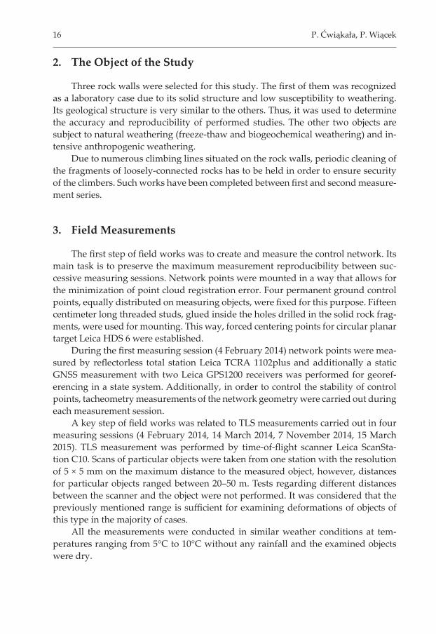
Laboratory case object is characterized by solid structure; therefore, it was as-sumed that expected compared values should be close to zero. Figure 1 shows the results obtained from diff erent methods of comparing point clouds with maximum density (5 mm), which are presented for the fragment of test object.

This is the area of the maximum variety of structure, and thereby it determines the biggest errors of the comparison. Despite the fi gures which show the image of the test object, the graphs showing the diff erences of distances between point clouds displayed by the amounts of points in a given range of diff erences were presented.

Applying the Nearest Neighbor method, the mean distance between point clouds reached the level of 5 mm with the standard deviation of ±2 mm. This result is based on point cloud density which was 5 mm. The greatest diff erences between point clouds appeared in rock depressions, where the diff erences between point clouds reached even up to 30 mm. Bett er results were obtained using the Least Square Plane and Height Function method for which the diff erence between point clouds amounted for 3 mm with its error value at ±2 mm. Similarly as in the case of the Nearest Neigh-bor method, it is noticeable that the biggest depressions of the objects are the places where the greatest errors with values over 10 mm appear. The 2.5D Triangulation method provided much bett er results with the diff erence between the point clouds on the level of 2 mm determined with the error of ±2 mm. What is more, this method enabled proper interpretation of rock depressions with irregular structure. However, noises and outliers are highly noticeable, which is visible as lighter points with the values up to 5 mm. As it was anticipated, the best results at the level of 0 ±1 mm were obtained with the use of the M3C2 method, which entirely eliminated the infl uence of noises. The errors in the biggest depressions reaching 5 mm are most likely caused by unequal covering of the object during subsequent measuring sessions. According to the authors, those errors should be regarded as random errors.

It was impossible to perform a TIN model comparison for original point clouds and available processing power. Therefore, a TIN comparison was initiated by fi l-tering primary point clouds up to 10 mm resolution. As in the 2.5D Triangulation method, errors and noises were not eliminated which results in single points of out-lier values. On the basis of this analysis, it was stated that the most suitable method for examining deformations of such objects is the M3C2 method.

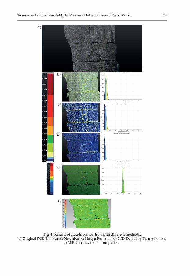
Next step of the analysis was to determine the optimum resolution which al-lows the fastest fi eld measurements and ensures the accuracy essential for exam-ining cavities on objects of this type. The analyses were conducted for fi ve cloud densities: original (ca. 5 mm), 10 mm, 25 mm, 50 mm and 100 mm. Taking into con-sideration the fact that scanning measurement was performed in GRID network, a similar method in GeoMagic program was adopted for unifying the point clouds.

Figure 2 shows the comparison of point clouds with diff erent density per-formed by using the M3C2 method. Irregular structure of the clouds with density up to 25 mm is clearly refl ected and signifi cant disturbances are not visible while calculating the diff erences.


Fig. 1. Results of clouds comparison with diff erent methods: a) Original RGB; b) Nearest Neighbor; c) Height Function; d) 2.5D Delaunay Triangulation;

e) M3C2; f) TIN model comparison

a)

b)

c)

d)

e)

f)


However, despite theoretical results at the level of 0 ±3 mm for 50 mm and 100 mm resolutions, it is visible that signifi cant diff erence values, which do not cor-respond with actual displacements, appear in the places of the most varied struc-ture. On the basis of this analysis, it was recognized that test objects of this type can be successfully measured with the resolution of up to 30 mm.

6. Calculating the Volume of Rock Cavities with Assessment of Accuracy

After choosing an adequate method of point cloud comparison, the analysis of accuracy of marking the volume of emerging rock cavities was performed. Taking into account the fact that no cavities developed between subsequent sessions, third and fourth, calculating diff erences should be close to zero. The calculations were performed in Surfer 9 program by Golden Software company. GRID network was created by Natural Neighbor interpolation method with 2 cm step. Due to the fact

Fig. 2. Results of clouds comparison using points cloud of diff erent density: a) 5 mm; b) 10 mm; c) 25 mm; d) 50 mm; e) 100 mm

a) b) c)

d) e)


that the algorithm of the program calculates the volumes along Z axis, it was neces-sary to transform the point clouds to make it maximally parallel to the plane created by X and Y axes. After creating GRID network for both measuring sessions, their range was limited to the area of examined object and then the volume between par-ticular GRID networks was determined. Obtained results are presented in Table 3.

Table 3. Volumes of emerging rock cavities calculated for point clouds of diff erent densities

Positive [m3] Negative [m3] Net [m3] Area [m2]Relative error

3

2

mm

positive negative

Original 0.061 0.094 −0.033 67.5 0.0009 0.0014

10 mm 0.064 0.091 −0.027 67.5 0.0009 0.0013

25 mm 0.066 0.097 −0.031 67.5 0.0010 0.0014

50 mm 0.088 0.132 −0.044 67.5 0.0013 0.0020

100 mm 0.12 0.167 −0.047 67.5 0.0018 0.0025

Avg. 0.080 0.116 −0.036 – 0.0015

Std. dev 0.022 0.029 0.008 – 0.0005

Computed volumes for density ranges under 25 mm adopted the values of ca. 0.03 m³ and ca. 0.05 m³ for the clouds with the density of 50 mm and 100 mm. Therefore, it was recognized that obtained volumes result merely from measure-ment and computing errors. On the basis of these calculations, it was possible to determine volume relative error which was identifi ed as a quotient of obtained vol-umes and surface area of test object. After averaging all the results, the value of 0.0015 ±0.0005 was obtained. Similar calculations were conducted for models created in Geomagic program. It provided the results in a range of 0.1–0.2 m³ which, com-paring to earlier outcomes, is a far worse result. Therefore, the volumes of cavities of remaining objects were calculated in Surfer.

7. Results

After establishing all parameters of accuracy of conducted measurements for the test object, two remaining areas were examined. However, before comparing them, it was necessary to fi lter the point clouds from vegetation situated on the ob-ject in the fi rst place. In order to obtain the best results, manual fi ltering was carried out in Leica Cyclone program. Subsequently, the comparison of distances between


point clouds for object no. 2 was performed (Figs 3, 4). This comparison enables indication of signifi cant cavities which developed between the fi rst and the second measurement session and reach up to 50 cm. Furthermore, a few smaller but signif-icant cavities were detected between the third and the fourth session. No signifi cant deformations were noticed between second and third session. It is worth pointing out that it is possible to observe single, minor cavities of even 1 cm.

Fig. 3. Object no. 2 Comparison of the fi rst and the second session

Fig. 4. Object no. 2 Comparison od the third and the fourth session


Afterwards, the changes of volumes for the whole object and four areas with major changes were calculated. The calculations were performed for all combina-tions of measurement series. On the basis of positive volumes, which were consid-ered to be caused by measurement errors and fi ltering, relative volume error and error limit value for signifi cant changes were calculated.

These values were calculated as:

( 2.5 )v e dS R S A ,

where: Sv – signifi cant value [m3],

Re – relative error 3

2

mm

,

Sd – standard deviation calculated from all relative errors 3

2

mm

, A – calculated area [m2].

Relative error value was assigned as quotient of positive volumes and surface area obtained for all compared areas and combinations of the compared session. Thus, a 30 values (fi ve compared areas and six combination of compared session) for object no. 2 and 24 (four compared areas and six combination of compared session) for object no. 3 was determined. After that average value and it standard deviation was calculated and used to determine the limit error of signifi cant error.

This provided the results presented in Table 4.

Table 4. Volume results for object no. 2

Sess

ion

Whole object Area 1 Area 2 Area 3 Area 4

ΔV [m3]

signif-icant value [m3]

ΔV [m3]


ΔV [m3]

signifi cant value [m3]

ΔV [m3]


ΔV [m3]


2–1 −2.1864

±1.2529

−1.0516

±0.0404

−0.2502

±0.0126

−0.0044 0.0065 −0.0063

±0.04923–2 0.2311 −0.0022 −0.0007 0.0013 0.0065 0.0062

4–3 −0.0605 −0.0029 0.0015 −0.0398 0.0065 −0.0239

Area [m2] 229.4 7.4 2.3 1.1 6

Relative error 3

2

mm

0.0022 Average value

±0.0013 Standard deviation


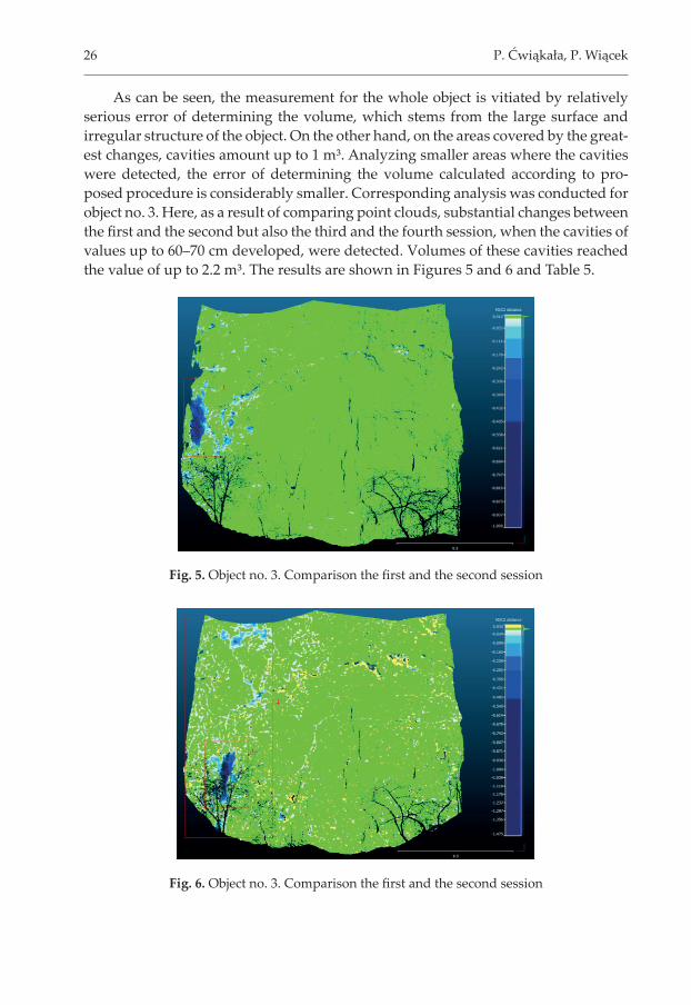
As can be seen, the measurement for the whole object is vitiated by relatively serious error of determining the volume, which stems from the large surface and irregular structure of the object. On the other hand, on the areas covered by the great-est changes, cavities amount up to 1 m³. Analyzing smaller areas where the cavities were detected, the error of determining the volume calculated according to pro-posed procedure is considerably smaller. Corresponding analysis was conducted for object no. 3. Here, as a result of comparing point clouds, substantial changes between the fi rst and the second but also the third and the fourth session, when the cavities of values up to 60–70 cm developed, were detected. Volumes of these cavities reached the value of up to 2.2 m³. The results are shown in Figures 5 and 6 and Table 5.

Fig. 5. Object no. 3. Comparison the fi rst and the second session

Fig. 6. Object no. 3. Comparison the fi rst and the second session


Table 5. Volume results for object no. 3

Session

Whole object Area 1 Area 2 Area 3

ΔV [m3] signifi cant value [m3] ΔV [m3] signifi cant

value [m3] ΔV [m3] signifi cant value [m3] ΔV [m3] signifi cant

value [m3]

2–1 −2.1413

±3.5618

−1.7520

±0.0826

−2.2189

±0.4917

−0.3682

±0.20973−2 0.1737 −0.0040 0.0284 0.0069

4−3 −2.6391 −0.0601 −1.7256 −1.4756

Area [m2] 383.9 8.9 53 22.6

Relative error []0.0040 Average [m3/m2]

±0.0021 Standard deviation [m3/m2]

8. Conclusions

On the basis of obtained results, laser scanning method may be considered as highly useful for measuring the volume and deformations of rock cavities. It allows for marking deformations even with a few millimeters accuracy and, at the same time, provides the full image of developed changes. However, it has to be noted that in order to obtain reliable results, the maximum reproducibility of conducted mea-surements and adequate method of point cloud comparison has to be adopted. At the same time, it is possible to precisely defi ne the volume of remaining cavities. In this case, the best solution is to carry out the measurements only for the areas where the cavities were previously identifi ed.

References

[1] Zagrożenia naturalne w odkrywkowych zakładach górniczych. Wyższy Urząd Górniczy, Katowice 2007.

[2] Girard J.M.: Assessing and monitoring open pit mine highwalls. [in:] Proceedings of the 32nd Annual Institute on Mining Health, Safety and Research, Salt Lake City, Utah, August 5–7, 2001, University of Utah, Salt Lake City 2001, pp. 159–171.

[3] Hearn G.J.: Slope Engineering for Mountain Roads. Geological Society Engi-neering Geology Special Publication, vol. 24, Geological Society of London, London 2001.


[4] Olek B., Woźniak H., Stanisz J.: Statistical methods used for determining geo-technical parameters. Przegląd Geologiczny, r. 62, nr 10/2, 2014, pp. 657–663.

[5] Motyka J., Czop M.: Vertical Changes of Iron and Manganese Concentration in Water from Abandoned “Zakrzówek” Limestone Quarry near Cracow (South Po-land). [in:] Mine water and the environment: proceedings of the 10th IMWA con-gress 2008: 2–5 June, 2008, Karlovy Vary, Czech Republic, VSB – Technical Uni-versity of Ostrava, Ostrava, pp. 167–170.

[6] Alba M., Fregonese L., Prandi F., Scaioni M., Valgoi P.: Structural Monitoring of Large Dam by Terrestrial Laser Scanning. [in:] Proceedings of the ISPRS Com-mission V Symposium “Image Engineering and Vision Metrology”: Remote Sens-ing and Spatial Information Sciences, vol. 36, part 5, pp. 1–6, September 25–27, 2006 Dresden, Germany.

[7] Lague D., Brodu N., Leroux J.: Accurate 3D comparison of complex topography with terrestrial laser scanner: application to the Rangitikei canyon (N−Z). ISPRS Journal of Photogrammetry and Remote Sensing, vol. 82, 2013, pp. 10–26.

[8] CloudCompare v2.6.1 Documentation.[9] Girardeau-Montaut D., Roux M., Marc R., Thibault G.: Change detection on

points cloud data acquired with a ground laser scanner. [in:] ISPRS Workshop Laser Scanning 2005: Enschede, the Netherlands, 12–14 September 2005, GITC, pp. 30–35.

Assessment of the Possibility to Measure Deformations of...

Documents

Transcript of Assessment of the Possibility to Measure Deformations of...