Assessment of the parameter estimation capabilities of gPROMS ...

Graduation report

Professor: Prof. Dr. Ir. M. Steinbuch

Supervisors: Prof. Dr. Ir. A.C.P.M. Backx

Ir. G.M.P. Perkins

Eindhoven Technical University

Department Mechanical Engineering

Dynamics and Control Technology Group

Amsterdam, July 2005

Assessment of the parameter estimation

capabilities of gPROMS and Aspen

Custom Modeler, using the Sec-Butyl-

Alcohol stripper kinetics case study

Peter Tijl

DCT 2005.96

2

Summary

In order to optimize the chemical process that occurs in the Sec-Butyl-Alcohol (SBA)

stripper operated by Shell in Pernis, the kinetic parameters of the relevant reaction

scheme are required. For this purpose laboratory experiments have previously been

performed and modelled with Aspen Custom Modeler (ACM), a commercially available

software package developed by AspenTech. The objective of this graduation project is to

build a second model of the experiments using the gPROMS software package, which is

developed by Process Systems Enterprise (PSE), subsequently perform parameter

estimation with both software tools and assess their capabilities. Both experiment models

should be as similar as possible to allow for a comparative assessment. Therefore, the

physical and thermodynamic properties of the components in ACM are made available to

the gPROMS model via the CAPE-OPEN interface, which is successfully applied. The

experiment model developed in gPROMS consists of a vapour-liquid equilibrium that

describes the distribution of nine components with reactions taking place in the liquid

phase. The model responses are found to be very similar to the existing ACM model.

During parameter estimation it became clear that not all the kinetic parameter of the

proposed reaction scheme are individually observable in combination with the available

experiment data. Therefore, the system is partially reparameterised and the parameters

are determined with sufficient accuracy. Various aspects of parameter estimation are

assessed, such as: experiment data input, output interpretation, available combinations of

objective functions and optimization solvers and their ability, speed and accuracy of

obtaining a solution. From this work it is concluded that the parameter estimation

capabilities of gPROMS are better than ACM. Additionally, it is investigated what type

of experiments are required in order to obtain parameters that remained unobservable

with the current experiment data. Attempts to apply the gPROMS Sequential Experiment

Design (SED) were unsuccessful and the added value of the SED functionality could not

be assessed. Alternatively designed experiments are simulated with a model that contains

known kinetic parameters and subsequently this synthetic experiment data is used to

estimate the parameters. The effect of data reduction on the observability of the

parameters is investigated. It proved to be possible to estimate all parameters in three

different reaction systems using a reduced set of synthesized experiment data.

3

Table of contents

SUMMARY ................................................................................ 2

TABLE OF CONTENTS.............................................................. 3

1 INTRODUCTION ................................................................. 5

2 PROJECT OBJECTIVES ....................................................... 6

3 ASSESSMENT CRITERIA .................................................... 7

3.1 MODEL BUILDING ........................................................................................................................ 8 3.2 PARAMETER ESTIMATION............................................................................................................ 8 3.3 EXPERIMENT DESIGN................................................................................................................... 9

4 CASE STUDY .....................................................................11

4.1 PROCESS DESCRIPTION ............................................................................................................ 11 4.2 LABORATORY EXPERIMENTS .................................................................................................... 12 4.3 REACTION SCHEME ................................................................................................................... 13 4.4 COMPONENTS AND INTERMEDIATES ......................................................................................... 14

5 MODEL BUILDING.............................................................16

5.1 ESSENTIAL SYSTEM EQUATIONS............................................................................................... 16 5.2 THE CAPE-OPEN INTERFACE ................................................................................................ 19 5.3 THE VAPOUR-LIQUID EQUILIBRIUM (VLE) ................................................................................ 19

5.3.1 Implementation ..................................................................................................................... 21 5.4 EXPERIMENT DATA INPUT ......................................................................................................... 23 5.5 ASSESSMENT ON MODEL BUILDING .......................................................................................... 26

6 PARAMETER ESTIMATION ................................................28

6.1 REACTION KINETICS .................................................................................................................. 28 6.1.1 Reaction kinetics reduced scheme ........................................................................................ 29 6.1.2 Reaction kinetics complete scheme....................................................................................... 34

6.2 SOLVING METHODS ................................................................................................................... 42 6.2.1 Objective functions ............................................................................................................... 42 6.2.2 Optimisation solvers ............................................................................................................. 45

6.3 PERFORMANCE ......................................................................................................................... 47 6.3.1 Ability and speed .................................................................................................................. 47 6.3.2 Accuracy ............................................................................................................................... 48 6.3.3 Effect of optimisation tolerance............................................................................................ 50

6.4 OUTPUT INTERPRETATION ........................................................................................................ 51 6.4.1 Overlay plots......................................................................................................................... 52 6.4.2 Statistical analysis ................................................................................................................ 54

6.5 ASSESSMENT ON PARAMETER ESTIMATION ............................................................................. 56

7 EXPERIMENT DESIGN.......................................................58

7.1 INTRODUCTION .......................................................................................................................... 58 7.2 APPROACH ................................................................................................................................ 59 7.3 TRIANGLE REACTION SCHEME .................................................................................................. 60 7.4 CONSTRAINTS ........................................................................................................................... 64

7.4.1 Reduced measurement data .................................................................................................. 65

4

7.4.2 Effect of measurement error ................................................................................................. 67 7.5 CONCLUSIONS ON EXPERIMENT DESIGN................................................................................... 67

8 CONCLUSIONS..................................................................69

REFERENCES ..........................................................................70

NOMENCLATURE.....................................................................72

POINTING FACTOR .....................................................................72

APPENDIX A CHEMICAL STRUCTURES OF COMPONENTS...75

APPENDIX B HAMMETT ACIDITY ..........................................76

SAMENVATTING .....................................................................77

5

1 Introduction

In the petrochemical process industry there is an increasing challenge to improve

efficiency and reduce costs due to tight margins, a maturing business and environmental

legislation. An important method to face this challenge is process modeling with the use

of so-called Computer Aided Process Engineering (CAPE) tools. These CAPE tools are

extensively used in the design, operation and optimisation of chemical processes. In order

to obtain useful models that can be applied to design optimisation, values of unknown

parameters relating to chemical kinetics must be obtained from laboratory or plant data.

The process of formulating a model and determining unknown parameters is referred to

as model development and is investigated in this project.

Multiple commercial developers of CAPE tools exist and each software package has it’s

own specific functionalities. In this project the model development and parameter

estimation capabilities of two widely used commercial software packages are assessed

and compared from a user point of view. The two packages are Aspen Custom Modeler

11.1 developed by AspenTech and gPROMS 2.3.3 developed by Process Systems

Enterprise. Both software programs have previously been reviewed by the Eurokin

consortium [8] however, with test cases that were not very challenging. The case study

applied to assess and compare the model development capabilities of both CAPE tools in

this project is a realistic and industrially relevant example. In the case study the aim is to

obtain the unknown kinetic parameters of the reactions taking place in the Sec-Butyl

Alcohol (SBA) stripper, operated by Shell. Experiments have been performed on

laboratory scale and a dynamic model of these experiments is built to fit the experiment

data.

The outline of this report is as follows: In chapter 2 the project objectives are identified.

Next, the process of model development is presented and the criteria used to asses both

software packages are defined at the various model development stages in chapter 3. In

chapter 4, the case study that is applied to investigate the model development capabilities

is described in terms of the actual process and the laboratory experiments. Chapter 5

elaborates on how the model is developed in gPROMS. The unknown parameters in this

model are estimated as described in chapter 6. Most of this work is also performed in

Aspen Custom Modeler (ACM) and at the end of chapters 5 and 6 the model

development capabilities of gPROMS are assessed and where possible compared with

ACM. In chapter 7 it is investigated what type of experiments are required to obtain the

kinetic parameters. Finally, the conclusions that are drawn from the assessment are

presented.

6

2 Project objectives

An important objective of a company in the petrochemical process industry is to optimize

chemical processes and their operation. Therefore, it is essential to have insight into the

process of interest, in particular, to understand which chemical reactions take place and

what the accessory reaction kinetics are. A method frequently used in practice to obtain

the reaction scheme and its kinetic parameters is to model the system and perform

parameter estimation with the use of CAPE software tools [4]. A number of such

commercial software packages exist; two widely used tools are gPROMS and Aspen

Custom Modeler. The main objective of this project is to:

Assess the parameter estimation capabilities of the gPROMS software and

compare them with the Aspen Custom Modeler software, using a realistic

industrial process as case study, which is the Sec-Butyl-Alcohol stripper.

At the start of this project, laboratory experiment data and an experiment model in the

ACM software with the necessary physical properties of the components were available.

Furthermore, a reaction scheme was proposed that was assumed to describe the reactions

taking place both in the actual stripper process and in the laboratory experiments. The

main objective is divided into three underlying objectives, followed by a brief

explanation:

1. Develop an experiment model in gPROMS similar to the existing model in ACM,

applying the CAPE-OPEN interface to ensure identical physical properties.

In order to compare the model development capabilities of both software packages, it is

essential to use two identical experiment models with identical physical properties. The

exchange of physical properties between the two software packages should be possible

via the so-called CAPE-OPEN interface.

2. Perform parameter estimation to obtain a unique reaction scheme and its kinetic

parameters with both software packages and compare their performance and

usability.

A unique reaction scheme implies that a model response is the result of a unique set of

model parameters only. The criteria used to assess and compare the performance and

usability of both software packages are introduced in the next chapter.

3. Investigate what type of experiments is required to obtain the parameters

preferably by applying the gPROMS Sequential Experiment Design functionality

The gPROMS software has an extra functionality compared to the ACM software, which

is Sequential Experiment Design (SED) [20]. This would enable the user to sequentially

design future experiments such that the experiment data, used to improve the accuracy of

previously estimated parameters, has maximal information content. Then the response of

the system is such that the parameters become more observable.

7

3 Assessment criteria

In this chapter the criteria used to assess and compare the model development capabilities

of both software packages are introduced by walking through the process of model

development as schematically presented in Figure 3.1. Each step involving the use of a

CAPE tool is briefly discussed and the criteria relevant for that step are defined.

Figure 3.1 Schematic representation of model development.

Start

Model

kin data

phys.

Parameter

Estimation

Good fit?

Parameter

accuracy ok?

One clearly best

candidate model?

Finished

Alternative

kinetic scheme

Perform

experiment

Experiment

Design

parameter

precision

model

discrimination

yes

no

no

yes

yes

no

no

8

3.1 Model building

Assuming an experiment is already performed, the first stage in the model development

process is the building of a model that describes the performed experiments. In this

context, a model is referred to as a mathematical system of equations and variables that

describes the behaviour of a physical system. Typical items present in a model that

describes chemical experiments carried out to obtain a unique reaction scheme and its

kinetic parameters are: equations of conservation of mass and individual components

according to a reaction scheme with kinetic parameters, physical properties of the

components and the experiment data required to perform parameter estimation. The

criteria used to evaluate both packages in the model building section are related to the

latter two typical items of an experiment model:

• CAPE-OPEN compliancy; can the physical properties available in the ACM

environment be applied in the gPROMS software via the CAPE-OPEN interface?

• Interaction with MS Excel for experiment data input.

Other aspects such as programming effort and syntax are not taken into account since

they are very similar. Furthermore, the user is expected to have basic knowledge and

skills in model building, which is required for applying both software tools.

3.2 Parameter estimation

When the experiments are performed and a model of these experiments is built, the next

stage in the model development process is the estimation of unknown model parameters.

The software tools apply a mathematical routine that optimizes the fit of the model

response to measured values from the experiment data by varying certain model

parameters. The criterion for what is an optimal fit is defined by a so-called objective

function. The mathematical routine used to minimize the objective function by moving

the model parameters from an initial guess to their optimal values is referred to as the

optimisation solver. The first criterion used to evaluate both packages in the parameter

estimation section is:

• Ability and speed of obtaining optimal values for kinetic parameters

If the parameter estimation routine has found an optimal solution of the model

parameters, critical questions need to be asked that can hopefully be answered by correct

interpretation of the output provided by the software package. Correct interpretation of

the parameter estimation output depends on the skills and knowledge of the user, but also

on the amount, type and presentation of the statistical output provided by the software

package.

Good fit? The first aspect of the parameter estimation solution that has to be

investigated is the goodness of fit. This can be done by making an overlay plot of the

9

measured and predicted values of the experiment values. When the predicted values do

not match the measured values at all, this indicates that the model cannot describe the

actual process. Assuming other model aspects are correct, the proposed solution is to

generate an alternative kinetic scheme that does represent the reaction mechanism taking

place in the chemical process. The criterion to evaluate both software tools in the output

interpretation stage with regard to this first critical question is:

• Accessibility and functionalities of overlay plots.

Parameter accuracy ok? If the goodness of fit is satisfactory, the second aspect in

interpreting the parameter estimation output is the parameter accuracy. The accuracy is

usually presented in terms of the standard deviation of an estimated parameter and a

confidence interval with a percentage of certainty that the actual parameter value is

within that interval. The reason for possible unsatisfactory parameter accuracy is that the

experiment data does not contain sufficient information to accurately determine the

model parameters. There are two approaches to tackle this problem; the first one is to

design one or more new experiments that, in combination with the already available

measurement data, do contain sufficient information. This approach is discussed in more

detail in the next stage of model development, experiment design. Secondly, the model

can be re-parameterised, reducing the number of parameters to be estimated. Assuming

other model aspects are correct this can result in a reduced kinetic scheme with less or

other reactions then the initial scheme. However, it can also be the case that some

parameters cannot be determined individually because they become clustered in the rate

equations, this then becomes apparent by high cross-correlations of the parameters

involved. The group of clustered parameters can be replaced by a single parameter that

can probably be determined with sufficient accuracy. Alternatively, all but one of the

parameters that are clustered can be set to a fixed value. All these forms of re-

parameterisation reduce the number of parameters to be estimated. To indicate the reason

for unsatisfactory parameter accuracy and deciding which parameters are redundant

requires detailed knowledge of the reaction system and is usually not straightforward.

The criteria used to assess and compare both software packages in the output

interpretation stage regarding parameter accuracy are:

• Level of accuracy achieved compared to estimated value of parameter.

• Available statistical information.

3.3 Experiment design

When the parameter accuracy is unsatisfactory or when it is not clear which of multiple

candidate models is superior, one or more new experiments need to be performed. Since

performing experiments is usually costly and time consuming, it is required they are

designed as efficiently as possible. Here, efficiently means that the experiment data

contains maximal information to either improve the parameter accuracy or distinguish

10

between candidate models. The criteria used to assess and compare both software

packages in the experiment design stage of the model development process are:

• Availability and functionality of experiment design for parameter precision.

• Added value of the experiment design feature.

The last criterion is difficult to assess without walking through the following steps:

perform an experiment designed by the software packages and an experiment designed

intuitively, make an iteration by performing parameter estimation with the extra data

from both experiments and finally evaluating whether the parameter accuracy or model

discrimination is significantly better in the case of the experiments designed by the

software package based on statistical methods. It was however not possible to perform

new experiments in the scope of this project, therefore other methods need to be found to

evaluate the added value of experiment design by CAPE tools. This is discussed in more

detail in chapter 7.

11

4 Case study

The case study investigated to compare the model development capabilities of the two

software packages gPROMS and ACM, is a realistic industrial case. It involves the

stripper section of the production process of Secondary-Butyl Alcohol (SBA). In order to

obtain the reaction scheme and the intrinsic kinetics parameters of the reactions taking

place in the SBA stripper section, batch experiments have been performed in a laboratory

and a model that describes these experiments has been developed and validated with the

available experiment data. In the model development process, the kinetic parameters are

determined using the parameter estimation functionalities in both commercial modeling

software tools gPROMS and ACM.

In this chapter, first a short description of the actual production process of SBA is

presented, followed by a description of the conducted laboratory experiments used in this

case study. Next, the kinetic scheme of the reactions expected to take place during both

the actual process and the experiments is discussed and finally an overview is given of

the components involved in these reactions.

4.1 Process description

The COF/2 unit at Pernis produces SBA, precursor to Methyl Ethyl Ketone (MEK), by

hydration of Butene (C4) in the presence of sulphuric acid (H2SO4). In the reaction

section liquid C4 is reacted with 72% sulphuric acid at 40 to 55 ºC, thereby forming so-

called fat acid containing SBA in free form and as Mono-Butyl Sulphate (MBS). This acid

is hydrolysed by the addition of water in the hydrolysis section, after which it is fed into

the stripper section. Low-pressure steam as a stripper medium enters the stripping

columns from the bottom. SBA and other light components, such as various butenes, are

drawn off at the top vapour outlet and diluted sulphuric acid or spent acid is drawn off at

the bottom liquid outlet. All light components drawn off are fed into the next section,

where caustic is used to neutralize any residual acid. Spent acid is sent to the Mantius,

where it is re-concentrated to approximately 72% acid strength, after which it can be re-

used in the reaction section [7].

The focus in this project is on the stripper section. The SBA stripper is a reactive

distillation column in which, as the products are being removed by distillation, the MBS

to SBA hydrolysis equilibrium is shifted towards the alcohol. Not only does the desired

hydrolysis reaction take place in the stripper, but also the undesirable reversion of MBS

and SBA to butanes. Roughly 25 to 30% of the potential alcohol is turned into reversion

gas that must be recycled to the reactors.

The objective in the case study is to obtain the reaction scheme and its kinetic parameters,

which will be used in a later stage to improve understanding in how to manipulate the

stripper operating variables such that the formation of reversion gas is minimized.

12

4.2 Laboratory experiments

The laboratory batch experiments were carried out using a “Hastelloy-C bolted-head”

autoclave with a total blocked-in volume, which includes the liquid phase and the vapour

cap, of 1033.2 cc. A “Welker Cylinder” with a capacity of 500 cc was used as a feed

charging system for the transfer of butane/butene liquid feed into the autoclave. Samples

taken from the liquid phase in the autoclave were collected in stainless steel sample

bombs, using an automated sampling system, and were diluted with cyclohexane and

water [16]. A schematic representation of the experiment set-up is presented in Figure

4.1.

Figure 4.1 Schematic representation of experiment set-up.

Two types of experiments were carried out to determine the reaction kinetics. The first

type involves the (desired) hydrolysis of MBS via an intermediate to SBA. The second

type of experiments is the reverse of the first type, it is the (undesired) sulfation of SBA

via an intermediate to MBS. Both temperature and pressure are maintained constant

during individual experiments. In order to raise the temperature, a heating jacket was

used and the reactor was pressurized by adding nitrogen (N2) gas, which is inert.

In order for the experiment data to obtain information on the reaction activation energies,

it is required to have experiment data at multiple temperatures. Therefore, both the

hydrolysis and the sulfation experiments are performed at three temperatures: 60, 75 and

90 °C with various initial compositions. Unfortunately, the experiments could not be

performed at the actual process temperature of about 115 °C. At this temperature, the

reactions occur too fast for the equipment to take multiple samples during the transient

behaviour of the reactions. Capturing the transient behaviour is essential to determine the

kinetic parameters that describe the reaction dynamics.

13

A total of 19 experiments have been performed, named “exp097” increasing in number

up to “exp115”. They are distinguished into two different types and three different

temperatures, as presented in Table 4.1. Five samples from the liquid phase are taken

during each experiment and the composition in terms of weight percentage of seven

components is measured, resulting in 665 data points. The weight percentage of the eight’

component (water) is determined indirectly, satisfying the constraint that the weight of all

eight components together is 100% of the total weight.

Table 4.1 Overview of experiments used in case study.

Sulfation Hydrolysis

exp097 exp104

exp099 exp105

exp112 exp106 T = 60 °C

exp115

exp098 exp107

exp100 exp108

exp101 exp109

exp113

T = 75 °C

exp114

exp102 exp110 T = 90 °C

exp103 exp111

Additional experiments have been performed to investigate the vapour-liquid phase

distribution, in this case study only the experiments in Table 4.1 are made use of. Details

of the experiment procedures and the data obtained from the experiments in Table 4.1

and the additional vapour-liquid phase distribution experiments can be found in [16].

4.3 Reaction scheme

Multiple reaction schemes have been proposed to describe the reaction kinetics in both

the batch experiments and the actual stripper process. The reaction scheme applied for the

reaction section in previous work was adopted to describe the reactions in the stripper

section [16]. However, during model development it became clear that the kinetic

parameters of the initially proposed reaction scheme could not be obtained in

combination with the available measurement data. The original reaction scheme is

simplified by removing one reversible reaction in order to obtain a unique fit with the

available measurement data. In Chapter 7 it is investigated what type of experiments

would provide the data that is required to estimate the parameters of this reaction. The

reaction scheme used in this case study to compare both software tools is schematically

displayed in Figure 4.2.

14

C4⊕ SBE

SBA

H⊕H⊕

H⊕

H⊕

1-C4= T2-C4

= C2-C4=

SBAMBS

H2SO4 H2O

H⊕

H⊕

C4⊕ SBE

SBA

H⊕H⊕

H⊕

H⊕

1-C4= T2-C4

= C2-C4=

SBAMBS

H2SO4 H2O

H⊕

H⊕

Figure 4.2 Schematic representation of reaction scheme

All the reactions that occur in the reaction scheme as presented in Figure 4.3 are

reversible and take place in the liquid phase. The reaction rate constants ki are presented

in brackets where the first of the two reaction rate constants belongs to the forward

reaction rate.

1-C4 + H+ C4

+ (k1 and k2)

c2-C4 + H+ C4+ (k3 and k4)

t2-C4 + H+ C4+ (k5 and k6)

C4+ + H2SO4 MBS + H+ (k7 and k8)

C4+ + H2O SBA + H+ (k9 and k10)

C4+ + SBA SBE + H+ (k11 and k12)

Figure 4.3 Reaction scheme.

A description of the components and intermediates that occur in the reaction scheme is

presented in the following paragraph.

4.4 Components and intermediates

In Table 4.2 an overview is provided of the components and intermediates C4+ and H

+

that are present in the reaction scheme. During the experiments the tank is pressurized

with the inert nitrogen gas, therefore this component is included in the overview as well.

15

Table 4.2 Overview of components and intermediates.

Abbreviation Full name Chemical formula

H2O Water H2O

H2SO4 Sulphuric acid H2SO4

SBA Sec-Butyl Alcohol C4H10O

MBS Mono-Sec-Butyl Sulfate C4H10O4S

SBE Sec-Butyl Ether C8H18O

C4+

Protonated Butene C4H9

1-C4 1-Butene C4H8

c2-C4 Cis-2-Butene C4H8

t2-C4 Trans-2-Butene C4H8

H +

Proton H

N2 Nitrogen N2

The chemical structures of the components in Table 4.2 are displayed in Appendix A.

16

5 Model building

The first stage in the model development process is model building. A model is defined

as a system of equations that describes the behaviour of a physical system in terms of

inputs, states and outputs. Before constructing a model it should be clear what it’s

purpose and requirements are. In this case, the purpose of the model is to determine the

unknown kinetic parameters of the reaction scheme that describes the SBA stripper

process. Therefore, batch experiments have been performed and the experiment model

will be validated using the experiment data, thereby determining optimal estimates of the

values for the intrinsic kinetic parameters.

The batch experiment model is required to describe the vapour-liquid equilibrium (VLE)

that exists in the CSTR and the reactions that take place in the liquid phase. Such an

experiment model has previously been built in ACM and a new, identical model needs to

be developed in gPROMS. Some challenging aspects in modelling the batch experiments

are the use of the CAPE-OPEN interface to describe the VLE and the fact that the amount

of nitrogen is a free variable that is determined by satisfying the constraint that the

pressure is fixed in every experiment. The VLE determines the component distribution

over a vapour and a liquid phase, which is commonly referred to as a flash calculation. In

this chapter, first the essential system of equations is described that is required to solve a

tank reactor model consisting of a vapour-liquid equilibrium, N components and R

reactions, making use of a CAPE-OPEN interface. Next, the implementation and use of

the CAPE-OPEN interface is described. Finally, the underlying theory of vapour-liquid

equilibria is addressed followed by a consideration on how the VLE is best implemented

in the gPROMS model in order to result in a component distribution over both phases

similar to what the existing ACM model predicts.

5.1 Essential system equations

The system of equations presented in this paragraph is the minimal set of equations

required to solve a tank reactor model consisting of a vapour-liquid equilibrium, N

components and R reactions, making use of a CAPE-OPEN interface. In order to be able

to perform a Degree Of Freedom (DOF) analysis, the variables introduced in Table 5.1

are assigned a certain status (Known, Unknown: Algebraic, Unknown: Differential or

Initial) according to the terminology used in gPROMS. In this system, the number of

moles of the Nth component (N2) has status Unknown: Algebraic and is a free variable.

Otherwise the system would be overspecified, since the temperature, the pressure and the

total volume of the tank all have status Known and are thus fixed. The reader is referred

to the nomenclature for a description of the symbols.

17

Table 5.1 Status of essential model variables according to gPROMS terminology.

Indices Variable status Symbol

component reaction

Known T ,P , TV , Li ,φ , Vi ,φ , Ln,υ , Vn,υ , ji ,υ , jia , , jA , jEa , gR Ni ,...,1= Rj ,...,1=

Unknown: Algebraic Tn , Nn , ix , iy , Lin , , Vin , , Ln , Vn , LV , VV , LiC , , jk Ni ,...,1= Rj ,...,1=

Unknown: Differential t

ni

∂

∂ 1,...,1 −= Ni

Initial in 1,...,1 −= Ni

Equations (5.1) up to and including (5.16) represent the core of the experiment model

developed in gPROMS. As follows from the DOF analysis in Table 5.2 they form a

consistent set, which is a necessary requirement since all model equations are solved

simultaneously and most equations are implicitly solved. The conservation of the number

of moles is given by

∑=

=N

i

iT nn1

(5.1)

∑=

=N

i

LiL nn1

, (5.2)

∑=

=N

i

ViV nn1

, (5.3)

The liquid and vapour mole fractions are required to satisfy equations (5.4) up to and

including (5.11).

L

Li

in

nx

,= 1,...,1 −= Ni (5.4)

V

Vi

in

ny

,= 1,...,1 −= Ni (5.5)

11

=∑=

N

i

ix (5.6)

11

=∑=

N

i

iy (5.7)

18

ViLii nynxn ⋅+⋅= Ni ,...,1= (5.8)

The liquid and vapour mole fractions also appear as input variables for the CAPE-OPEN

interface, as is the case in equations (5.9) up to and including (5.11). The vapour-liquid

equilibrium is described by (5.9), as will be discussed in detail in paragraph 5.3.

( ) ( )iViiiLii yPTyxPTx ,,,, ,, φφ ⋅=⋅ Ni ,...,1= (5.9)

The liquid volume, the vapour volume and the total volume satisfy equations (5.10),

(5.11) and (5.12) respectively

( )iLnLL xPTnV ,,,υ⋅= Ni ,...,1= (5.10)

( )iVnVV yPTnV ,,,υ⋅= Ni ,...,1= (5.11)

VLT VVV += (5.12)

Equations (5.13) up to and including (5.16) are required to describe the change of the

number of moles in the liquid phase due to chemical reactions.

∑=

⋅⋅=∂

∂ R

j

jjiL

i rVt

n

1

,υ 1,...,1 −= Ni (5.13)

jiaN

i

Lijj Ckr,

1

,∏=

⋅= Rj ,...,1= (5.14)

TR

Ea

jj

j

eAk ⋅

−

⋅= Rj ,...,1= (5.15)

LiLLi CVn ,, ⋅= Ni ,...,1= (5.16)

In Table 5.2 a DOF analysis of equations (5.1) up to and including (5.16) is presented.

Table 5.2 DOF analysis.

Unknown: Algebraic 5N + 2R + 6

Differential N - 1 +

Total 6N + 2R + 5

Initial N - 1

Equations 6N + 2R + 5

19

As can be seen from the DOF analysis in Table 5.2, the total number of Unknown

variables is equal to the number of Equations. Furthermore, the number of Initial

variables equals the number of Differential variables. These two requirements have to be

met in order to have a well-posed system.

5.2 The CAPE-OPEN interface

The CAPE-OPEN (CO) thermodynamic and physical properties interface is applied in

order to guarantee that both the ACM and the gPROMS model make use of identical

thermodynamic methods and physical properties. This interface allows software

components that provide thermodynamic and physical properties calculations to be used

in a CAPE-OPEN compliant Simulation Environment (COSE). The essential

thermodynamic and physical properties data used in CAPE tools is also referred to as

basic data.

The basic data for the SBA process is exported from AspenPlus as a CO file with the

extension *.cota. While exporting, information is written in the MS Windows Registry

containing name, location and ProgId of the so-called Property Package (PP). A Property

Package is a complete, consistent, reusable and ready-to-use collection of methods,

chemical compounds and model parameters for calculating any of a set of known

properties for the phases of a material. It includes all the pure compound methods and

data, together with the relevant mixing rules and interaction parameters [19]. A collection

of PP’s is called a Property System (PS). In order to access the AspenTech PP in

gPROMS, it has to be introduced as a Foreign Object (FO). It then behaves as a sub-

model that makes use of methods (pre-defined functions) that usually require a certain

input (e.g. temperature, pressure, mole fraction) and return the value of the property

corresponding to the method.

The methods used in the gPROMS experiment model are: MolecularWeight,

LiquidFugacityCoefficient, VapourFugacityCoefficient, LiquidVolume and

VapourVolume. Not all existing methods are available in the CO PP that is generated by

AspenPlus. For instance, the method Kvalues that is commonly used to perform a flash

calculation and determine the Vapour-Liquid Equilibrium cannot be accessed. However,

as will follow in the next paragraph, there are many ways to describe the Vapour-Liquid

Equilibrium.

5.3 The vapour-liquid equilibrium (VLE)

For a mixture consisting N components, the liquid and vapour phase are in equilibrium if

the chemical potential of component i in the liquid phase is equal to the chemical

potential of component i in the vapour phase. Furthermore, it must hold that the

temperature and the pressure of both phases are equal [15]. Instead of the chemical

potential, another quantity is introduced named fugacity, for it is more directly related to

20

pressure and therefore often preferred in engineering calculations [15]. The fugacity is

related to the chemical potential by its definition

( ) ( ) ( )( )0,00

00,00

0

,,

,,ln,,,,

ii

ii

iiiixTPf

xTPfRTxTPxTP += µµ (5.17)

From which it follows that for a mixture to be in phase equilibrium, the fugacity of

component i in the liquid phase must be equal to the fugacity of component i in the

vapour phase, this is referred to as the isofugacity condition. Summarizing, a mixture

consisting of a liquid and a vapour phase is in phase equilibrium if the following

conditions are met:

( ) ( )iViiLi yTPfxTPf ,,,, ,, = (5.18)

VL TTT == (5.19)

VL PPP == (5.20)

Next, the fugacity coefficient is introduced for both the liquid and vapour phase defined

by respectively

Pxf iLiLi ⋅⋅= ,, φ ; Pyf iViVi ⋅⋅= ,, φ (5.21)

Combining (5.18) and (5.21) results in

iViiLi yx ⋅=⋅ ,, φφ (5.22)

The fugacity coefficients take account for the non-ideal behaviour of the phases. For an

ideal gas it holds that the vapour fugacity coefficient is one and that the vapour fugacity

of component i is equal to its partial pressure.

1, =Viφ ; iiVi PPyf ≡⋅=, (5.23)

The liquid fugacity is usually expressed in terms of an activity coefficient. This approach

makes the system suited for describing the interaction between multiple liquid phases that

occurs in liquid-liquid and vapour-liquid-liquid systems. The activity coefficient is

derived from the quantity activity, which is defined as the ratio of the actual fugacity and

a reference fugacity of the pure liquid at saturation pressure. The definitions for

respectively activity and activity coefficient are

( )( )0,0

0 ,,

,,

ii

ii

ixTPf

xTPfa ≡ (5.24)

21

i

i

ix

a≡γ (5.25)

Combining (5.24) and (5.25) results in the following expression for the liquid fugacity

0

,, LiiiLi fxf ⋅⋅= γ (5.26)

Furthermore it holds that

ifLi

sat

iLi Pf ,

0

,

0

, Ρ⋅⋅= φ (5.27)


ifLi

sat

iiiLi Pxf ,

0

,, Ρ⋅⋅⋅⋅= φγ (5.28)

We now have two different types of expressions for the liquid and the vapour fugacity,

which still need to satisfy the isofugacity condition in (5.18). Therefore, combining and

reorganising (5.18), (5.21) and (5.28) results in a more explicit form of the vapour-liquid

equilibrium equation

ifLiii

sat

iVii xPyP ,

0

,, Ρ⋅⋅⋅⋅=⋅⋅ φγφ (5.29)

This equation is generally valid at pressure conditions below 10 bar and it is the basis

from which approximations can be derived, such as Raoult’s law. Another feature of

equation (5.29) is that it reveals which types of Basic Data are used.

5.3.1 Implementation

The existing ACM model makes use of the Non-Random Two Liquid (NRTL) model that

computes the activity coefficient of the various components. This model is based on the

idea that on microscopic scale the local composition in a mixture deviates from the

overall composition due to intermolecular interaction. An important aspect of the NRTL

model is that it assumes the gas phase is ideal, resulting in a vapour fugacity coefficient

of one for all present components. Furthermore, the Poynting factor if ,Ρ , which is a

pressure correction factor, is also one for all present components. Thus when applying the

NRTL model, the vapour-liquid equilibrium equation (5.29) is reduced to

0

,Liii

sat

ii xPyP φγ ⋅⋅⋅=⋅ (5.30)

The most logical approach would be to implement equation (5.30) in the gPROMS model

as well. Therefore, all the variables apart from the mole fractions in both phases xi and yi

need to be known, since the relation between these fractions for all components is

22

required. The total pressure is known from the experiments and the liquid activity

coefficient together with the liquid fugacity coefficient at reference pressure are available

in the CO package exported from AspenPlus. The saturation pressure can also be

exported from AspenPlus in the CO package, it is however not available. In the ACM

model, the saturation pressure or vapour pressure of a pure component i is calculated as a

function of temperature and a set of seven coefficients, using the extended Antoine

equation. This correlation is also applied in the gPROMS model together with equation

(5.30) to describe the VLE. In order to test that the ACM and the gPROMS model give

similar results, flash calculations without any reactions have been performed. The results

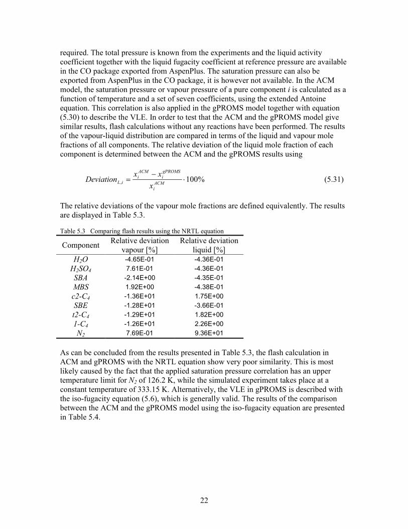
of the vapour-liquid distribution are compared in terms of the liquid and vapour mole

fractions of all components. The relative deviation of the liquid mole fraction of each

component is determined between the ACM and the gPROMS results using

%100, ⋅−

=ACM

i

gPROMS

i

ACM

iiL

x

xxDeviation (5.31)

The relative deviations of the vapour mole fractions are defined equivalently. The results

are displayed in Table 5.3.

Table 5.3 Comparing flash results using the NRTL equation

Component Relative deviation

vapour [%]

Relative deviation

liquid [%]

H2O -4.65E-01 -4.36E-01

H2SO4 7.61E-01 -4.36E-01

SBA -2.14E+00 -4.35E-01

MBS 1.92E+00 -4.38E-01

c2-C4 -1.36E+01 1.75E+00

SBE -1.28E+01 -3.66E-01

t2-C4 -1.29E+01 1.82E+00

1-C4 -1.26E+01 2.26E+00

N2 7.69E-01 9.36E+01

As can be concluded from the results presented in Table 5.3, the flash calculation in

ACM and gPROMS with the NRTL equation show very poor similarity. This is most

likely caused by the fact that the applied saturation pressure correlation has an upper

temperature limit for N2 of 126.2 K, while the simulated experiment takes place at a

constant temperature of 333.15 K. Alternatively, the VLE in gPROMS is described with

the iso-fugacity equation (5.6), which is generally valid. The results of the comparison

between the ACM and the gPROMS model using the iso-fugacity equation are presented

in Table 5.4.

23

Table 5.4 Comparing flash results using the iso-fugacity equation

Component Relative deviation

vapour [%]

Relative deviation

liquid [%]

H2O -8.54E-04 -6.93E-05

H2SO4 -3.20E-04 1.31E-04

SBA 4.03E-04 8.28E-05

MBS < 1E-08 -1.57E-03

c2-C4 -6.61E-04 -1.33E-03

SBE -5.68E-03 -3.35E-03

t2-C4 < 1E-08 8.61E-04

1-C4 < 1E-08 -3.36E-03

N2 -5.12E-05 < 1E-08

The flash calculation output of the ACM model and the gPROMS model using the iso-

fugacity equation is very similar, as can be seen in Table 5.4. The deviations are

considered to be small enough in order to assume that the flash calculation in both

models is identical. Summarizing, the vapour-liquid equilibrium is successfully modelled

in gPROMS using the iso-fugacity equation (5.22), where the fugacity coefficients are

provided through the CAPE-OPEN interface. The developed gPROMS experiment model

and the existing ACM experiment model are considered to be similar enough to perform

a comparative assessment with.

5.4 Experiment data input

In this paragraph the input of experiment data in both gPROMS and ACM is described.

This aspect is considered to be important, since large data sets are frequently encountered

and minor differences in the data input sequence can result in a large difference in

required time and effort.

ACM

Experiment data input in ACM is found under Tools, Estimation. This opens a window

with five tabs, one of which is named Dynamic Experiments. Behind this tab, the user can

introduce an experiment with a weighting factor. Furthermore there is a tick box that

indicates if the experiment is active, which means whether it is taken into account when

performing a parameter estimation run. Experiments can be copied as a whole within this

window, however not to another model. It is not possible to have more than one model

opened in an ACM session in general, but even when two sessions are opened it is not

possible to copy an experiment from one model to the other.

When an experiment is added, it can be edited by clicking Edit. This opens a window

with three tabs, being Measured Variables, Fixed Variables and Initial Variables. Behind

the latter tab, the user specifies the names and values of the variables that are indicated as

initial in the model. It is not possible to copy more than one value, from for instance MS

Excel, into this window. Behind the Fixed Variables tab, the user can specify variables

24

and corresponding values that maintain constant during an experiment, but can vary

between experiments. It is possible to specify time dependant values by selecting a Fixed

Variable and clicking Edit. This enables the user to assign certain values at certain points

in time for the Fixed Variable, with a linear change in time between the various points.

This is indicated with the word ramped where otherwise the value of the Fixed Variable

would appear, as can be seen in Figure 5.1.

Figure 5.1 Screenshot of ACM experiment data input for Fixed Variables.

Behind the Measured Variables tab the user can introduce the variable names followed

by clicking Edit, which opens a window where the actual measurement data input for a

specific experiment and a specific measured variable is required. A table appears from

which three columns can be edited: Time, Weight, and Observed Value. The measurement

weight is optional and can be specified for each individual measurement point. The other

columns (Predicted Value, Absolute Residual, % Residual and Standardized Residual)

are reserved for the results of a parameter estimation run and contain N/A when results

are not available. It is possible to paste two columns with values for the measurement

time and the corresponding observed value for each variable in each experiment.

However, it is not possible to paste measurement data for all measured variables of an

experiment at once, since the data for each measured variable is behind a separate

window.

gPROMS

A so-called project in gPROMS consists of multiple entities such as in this case the

variable types, a model entity with the system equations, a process entity to perform

simulation, an estimation entity and also experiment entities. The measured experiment

data is to be imported in these experiment entities. There is a distinction between

experiment entities for parameter estimation and for experiment design, in this paragraph

the setup of an experiment entity for parameter estimation is described.

25

One of aspects in which gPROMS differs from ACM is its accessibility and open code. A

good example is the experiment entity, which can be accessed and edited both through a

Graphical User Interface (GUI) and by using the gPROMS language. Both are different

representations of one item, therefore an action performed via the GUI is immediately

visible in the language and vise versa. Similar to ACM, the experiment entity contains

three tabs to specify initial conditions, constant or fixed variables and the measured data

itself. These three tabs are accessible via the GUI and the fourth tab contains the

gPROMS language representation of the first three tabs and thereby the entire experiment

entity. The fifth tab named properties contains general file information about the

experiment entity.

In the first tab named initial conditions, the user specifies the names and initial values of

the variables that have a time derivative in the model. In the second tab named controls,

the variable names and values of so-called time-invariant or piecewise constant controls

can be specified. The piecewise constant option enables the user to define a discontinuous

change of a variable with a zero order hold, opposed to a ramped change (first order hold

behaviour) in ACM. In the third tab named measured data, all measured variables and

their values at various points in time during one experiment can be defined in one table.

The complete table with values for all variables can be pasted from a spreadsheet in e.g.

MS Excel. There is an option to transpose the table in gPROMS, which can be useful

depending on how the raw experiment data is available. A measured variable and its data

can be ignored by commenting it out in the gPROMS language representation of the

experiment entity, which is behind the fourth tab. In the estimation entity the user

specifies which experiments to use for parameter estimation and it is straightforward to

exclude complete experiments here. Part of two experiment entities of experiments 97

and 98 is displayed in Figure 5.2. The measured data for experiment 97 is represented

through the GUI, for experiment 98 it is represented in the gPROMS language. The

project tree with its various previously discussed entities can be seen on the left.

Figure 5.2 Screenshot of gPROMS experiment data input entities for experiments 97 and 98.

26

5.5 Assessment on model building

A model of the laboratory batch experiments performed in a CSTR was available in

ACM and an equivalent model has been built in gPROMS. In these batch experiments

some components were significantly present in two phases and therefore a vapour-liquid

equilibrium is taken into account in both models. Part of a gPROMS library model is

used to incorporate this vapour-liquid equilibrium. The required thermodynamic and

physical properties of the components are made available through the CAPE-OPEN

interface. Furthermore, the dynamic experiment data is imported in both software tools.

In this paragraph an assessment is made of both software packages concerning the work

performed in the model building stage.

CAPE-OPEN

Both AspenTech and PSE claim that their software is fully CAPE-OPEN compliant,

however not all methods are supported by the property package exported from

AspenPlus. This was encountered when attempting to describe the vapour-liquid

equilibrium with the commonly used method named K-values. Furthermore, the method

Vapourpressure that is required when using the NRTL approach of describing the VLE,

returned values of 1e35 for all components, which cannot be trusted. Fortunately, the

methods LiquidFugacitycoeffient and VapourFugacitycoefficient are supported by the

property package, which makes it possible to describe the VLE with the iso-fugacity

equation. No compliancy problems were faced on the gPROMS side.

Another issue encountered using the CAPE-OPEN interface was the inability to set the

initial mass holdup of one or more components to zero. Even values smaller than 1e-5

caused gPROMS to fail during initialisation. No further investigation has been made to

whether the problem is on the gPROMS or on the AspenPlus side. The most robust

solution to this problem is to remove the redundant components and their thermodynamic

parameters in AspenPlus and export a new CAPE-OPEN package containing only the

components required in the model. When this solution is not possible for some reason, a

workaround is to run a simulation with the smallest values allowed and save the complete

variable set immediately after a successful initialisation. Use the saved variable set to

initialise a new simulation with smaller values for the components mass holdup where

necessary and again save the variable set just after initialisation. Repeating this procedure

eight times resulted in minimal values for the mass holdup of the relevant components of

1e-13 kg. The first, most robust solution is preferred and is applied in this work.

Summarizing, regarding the use of the CAPE-OPEN interface it is concluded that:

• The CAPE-OPEN thermodynamic and physical properties interface is

successfully applied to describe the vapour-liquid equilibrium.

• AspenPlus does not support all CAPE-OPEN methods when exporting a property

package.

27

• It is advised to remove redundant components and their binary interaction

parameters from a property package.

Experiment data input

What ACM and gPROMS have in common regarding experiment data input are the three

tabs where initial conditions, constant variables and measured variables and their

respective values are specified. For both software programs this can be done by copying

and pasting the values from a spreadsheet in e.g. MS Excel. A difference in the constant

variables tab is that ACM allows to specify constant and ramped (first order hold)

behaviour of a process variable e.g. temperature, where gPROMS has the option to

prescribe constant and piecewise constant (zero order hold) behaviour.

The most significant difference appears in the measured variables tab, where in gPROMS

it is possible to define all the variables and their values that are measured at various

points during the experiment. In ACM these values can be defined of one variable only as

a result of the structure where each variable in each experiment is accessed and edited in

a separate window. Due to this structure, 499 windows would have to be opened, edited

and closed in ACM opposed to 57 in gPROMS in order to perform the experiment data

input for this case study.

The software tools also differ regarding their options to exclude and re-include single

measurements, variables or complete experiments from a parameter estimation run.

Complete experiments can easily be in- or excluded in ACM by means of a tick-box

indicating whether an experiment is active. In gPROMS this can be done with similar

effort by placing or removing comment symbols {…} around or #… in front of the

experiment name in the estimation entity. The advantages of the having an open language

in gPROMS, which can also be represented and edited via a GUI, becomes clear when

excluding and re-including single measurements or measured variables. This can be done

in the language tab of an experiment entity, again by placing or removing comment

symbols. In ACM measured variables or single measurements can be removed from an

experiment via the GUI, this is however permanent and the measurement data is lost.

The conclusions drawn from comparing the experiment data input functionalities in ACM

and gPROMS are:

• Sets of measured values can be copied from a spreadsheet in e.g. MS Excel and

pasted into both software tools.

• The structure in ACM where each measured variable in each experiment is in a

separate window is very inconvenient for large data sets, in gPROMS all

measured variables and their values of an experiment are in a single table.

• Experiment data can easily be excluded and re-included in a parameter estimation

run in gPROMS due to its open language. Apart from complete experiments,

measured data can only be removed permanently and not re-included in ACM.

28

6 Parameter estimation

The various aspects of parameter estimation are discussed in this chapter. First the

development of the reaction scheme throughout the process of parameter estimation in

gPROMS is treated. Next, the solving methods of the two software packages are

highlighted in terms of the objective functions and the solvers that can be used to

minimize the objective function value. The performance of the various solving methods

is evaluated for three cases. The ability and the speed of the available solving methods to

find an optimal solution and the accuracy of the estimated parameters compared to their

standard deviations is assessed. For both software packages, their standard features for

the interpretation of the parameter estimation output results are investigated. Finally, the

conclusions drawn from these various aspects are summarized in the assessment

paragraph.

6.1 Reaction kinetics

The complete reaction scheme as introduced in paragraph 4.3 can be reduced to a

reaction scheme only taking into account the major components that are present in large

quantities in the liquid phase. Furthermore, from flash calculations it is concluded that

more than 99% of the total mixture is in the liquid phase. As a result of these

considerations, it is justified to approximate the kinetics of the reactions that involve the

major components by ignoring the reactions that are involved in forming the volatile

components. The reasons to simplify the kinetic scheme and perform model development

with this reduced scheme first, are to obtain insight in the process of model development

and to get initial guesses for the kinetic parameters of the reactions in the reduced scheme

when making the step to perform model development with the complete kinetic scheme.

Measurements at the end of a typical experiment show that the composition of the

mixture is such that four components are present in relatively large amounts, as can be

seen in Figure 6.1.

H20

H2SO4

SBA

MBS

SBE

t2-C4=

c2-C4=

1-C4=

Figure 6.1 Liquid mole composition in exp114 at t = 75 min.

29

6.1.1 Reaction kinetics reduced scheme

The reaction scheme is reduced to the reactions that involve the four major components

only, as presented in Figure 6.2. In order to maintain consistency with the complete

kinetic scheme, the numbering of the reaction rate constants is not changed.

C4

+ + H2SO4 MBS + H + (k7 and k8)

C4 + + H2O SBA + H + (k9 and k10)

Figure 6.2 Reduced reaction scheme.

The rate expressions for the components and the C4+ intermediate in the reduced scheme

are

]][[]][[ 8424742

++ +−= HMBSkSOHCkr SOH (6.1)

]][[]][[ 84247

++ −= HMBSkSOHCkrMBS (6.2)

]][[]][[ 102492

++ +−= HSBAkOHCkr OH (6.3)

]][[]][[ 10249

++ −= HSBAkOHCkrSBA (6.4)

=+4C

r ]][[]][[ 84247

++ +− HMBSkSOHCk (6.5)

]][[]][[ 10249

++ +− HSBAkOHCk

The concentration of the H+ intermediate is given by (6.6) where the Hammett acidity H0

is introduced, which follows from a correlation as presented in Appendix B.

010][

HH

−+ = (6.6)

The concentration of the C4+ intermediate cannot be measured directly or indirectly.

Therefore, the so-called Bodenstein approximation [11] is applied, which assumes that

the reaction rate of the intermediate is small and constant. In both the reduced and the

complete kinetic scheme these requirements are assumed to hold, resulting in

04

=+Cr (6.7)

Combining (6.5) with (6.7) and rearranging, results in the following expression for the

C4+ intermediate concentration

][][

][][][][

29427

108

4OHkSOHk

SBAkMBSkHC

+

+= ++ (6.8)

30

Next, this expression obtained as a result of the Bodenstein approximation is substituted

in the component rate expressions. Substituting (6.8) in (6.1) up to and including (6.4)

and rearranging results in component rate expressions that can be described by one

overall reaction rate r.

][][

]][[]][[][

29427

42107298

OHkSOHk

SBASOHkkMBSOHkkHr

+

−= + (6.9)

The component rate expressions are

rrr SBASOH ==42

(6.10)

rrr MBSOH −==2

(6.11)

The overall rate expression (6.9) is overparameterised, which becomes clear after

rearranging by dividing both numerator and denominator by k7. As can be seen from

equation (6.12), only three independent clusters of parameters appear, where there are

four individual parameters.

][][

]][[]][[

][

2

7

942

42102

7

98

OHk

kSOH

SBASOHkMBSOHk

kk

Hr

+

−

= + (6.12)

Applying the Bodenstein approximation reduced the number of independently observable

kinetic parameters by one. Instead of k7 and k9, only their ratio can be observed since

neither of both parameters appears individually in rate expression (6.12) and therefore the

parameter 9k ′ is introduced for which the following holds

7

9

9k

kk =′ (6.13)


][][

]][[]][[][

2942

4210298

OHkSOH

SBASOHkMBSOHkkHr

′+

−′= + (6.14)

This overall rate is used to describe the component rate expressions and parameter

estimation is performed with the measurement data at a temperature of 60 °C. The first

aspect that should be considered with regards to interpreting parameter estimation output

is the ability to fit trends in the measurements. The overlay plots show that the predicted

values agree sufficiently with the measured values to confirm a good fit. Next, the

parameter accuracy is investigated. In this work it is considered that a parameter is

31

estimated with sufficient accuracy if the standard deviation is at least one order of

magnitude lower than the value of the estimated parameter. Furthermore, gPROMS

performs a t-test to investigate the individual parameter accuracy and a summary of the

parameter estimation output file is presented in Table 6.1.

Table 6.1 Summary of gPROMS parameter estimation output at T = 60 °C

A 95% t-value for a parameter component smaller than the reference t-value indicates that the data is not sufficient to estimate this parameter precisely.

Parameter Optimal Estimate 95% Confidence

Interval 95% t-value

Standard Deviation

k8 4.818019E+00 2.431668E+05 1.981364E-05 1.228733E+05

k’9 1.564989E-07 7.854225E-03 1.992545E-05 3.968777E-03

k10 3.603384E-07 1.533570E-08 2.349671E+01 7.749199E-09

Reference t-value (95%): 1.657715E+00

The gPROMS output file indicates that not all parameter are estimated with sufficient

accuracy. This conclusion can be drawn both from applying the previously mentioned

criterion on the standard deviation and from the information about the performed t-test.

The reason for the parameter inaccuracy becomes clear when considering the

denominator of the overall rate equation (6.14). Both concentrations that appear in the

denominator are of equal order of magnitude in the applied experiment data, 9k ′ is estimated to be in the order of 1e-7, thus for this dataset the following holds

][][ 4229 SOHOHk <<′ (6.15)

Allowing the simplification of (6.14) to

][

]][[]][[][

42

4210298

SOH

SBASOHkMBSOHkkHr

−′= + (6.16)

Rate expression (6.16) is over-parameterised due to the clustering of k8 and 9k ′ and therefore these two parameters are not individually observable. It is important to note that

the reason for the unobservability in this case is the lack of information in the experiment

data, which is different from the reason why parameters k7 and k9 were individually

unobservable. This was a direct effect of applying the Bodenstein approximation as

previously explained. In order to obtain a unique fit the parameter 9k ′′ is introduced, where

7

98

989k

kkkkk

⋅=′⋅=′′ (6.17)

Combining (6.16) and (6.17) leads to

32

][

]][[]][[][

42

421029

SOH

SBASOHkMBSOHkHr

−′′= + (6.18)

With overall rate equation (6.18) an alternative kinetic scheme is proposed and again

parameter estimation is performed. The overlay plots show a good fit and next the

parameter accuracy is investigated. A summary of the output is presented in Table 6.2.

Table 6.2 Summary of gPROMS parameter estimation output



Standard Deviation

k’’9 7.540134E-07 6.935782E-09 1.087135E+02 3.504683E-09

k10 3.603376E-07 2.781764E-09 1.295357E+02 1.405638E-09


The 95% t-values of both estimated parameters are larger than the reference t-value,

indicating sufficient accuracy. This is confirmed by considering that the standard

deviation is more than two orders of magnitude lower than the estimated value. Note that

multiplying the previously estimated values of k8 and 9k ′ approximately gives the

estimated value of 9k ′′ . This explains why in estimating k8, 9k ′ and k10 the overlay plots

showed a good fit, although the parameters could not be obtained with sufficient

accuracy. We can now conclude that rate equation (6.18) in combination with (6.10) and

(6.11) describes the behaviour of the major components and that the kinetic parameters

9k ′′ and k10 can be determined accurately. Next, the values of 9k ′′ and k10 are estimated

using the experiments performed at the two other temperatures of 75 and 90 °C. An

overview of the results at the three different temperatures is presented in Table 6.3.

Table 6.3 Parameter estimation results for reduced scheme.

Temperature [°C] Parameter Optimal estimate Standard deviation

60 9k ′′ 7.540134E-07 3.504683E-09

k10 3.603376E-07 1.405638E-09

75 9k ′′ 6.282991E-06 5.263236E-08

k10 3.373953E-06 2.997604E-08

90 9k ′′ 3.320208E-05 4.056078E-07

k10 1.536291E-05 2.040826E-07

33

The parameter accuracy of both 9k ′′ and k10 is sufficient at all three temperatures since the

order of magnitude of the standard deviations is two orders of magnitude less than the

estimated values. Finally, the kinetic parameters of the Arrhenius equation that describes

the temperature dependant behaviour of ki need to be determined. The reaction rate ki of

reaction i depends on the reaction temperature T according to the Arrhenius equation

TR

E

ii

ia

ekk ⋅−

⋅=,

,0 (6.19)

Where R is the universal gas constant and k0,i and Ea,i respectively are the pre-exponential

factor and the activation energy of reaction i. As can be concluded from (6.19), the pre-

exponential factor k0,i is a reference ki at a temperature of infinity. It is better to re-

parameterise (6.19), introducing a different reference kref,i that is related to a reference

temperature Tref that can be chosen within the range of the actual experiment

temperatures [4], [8]. The re-parameterised Arrhenius equation is given by

−

⋅=TTR

E

irefi

ref

ia

ekk

11

,

,

(6.20)

This re-parameterised Arrhenius equation is introduced in the model and the kinetic

parameters kref,i and Ea,i are estimated using the experiment data from all three

temperatures and a reference temperature of Tref = 75 °C. The results are presented in

Table 6.4.

Table 6.4 Parameter estimation results for reduced scheme, all temperatures

Parameter Optimal estimate Standard deviation

9,refk ′′ 5.696409E-06 3.005909E-08

kref,10 2.850522E-06 1.594955E-08

9,aE ′′ 1.330211E+05 3.907733E+02

Ea,10 1.322812E+05 3.906087E+02

Again sufficient accuracy is achieved and with these four parameters the time dependent

and the temperature dependant behaviour of the major components in all experiments

using the reduced reaction scheme is described.

34

6.1.2 Reaction kinetics complete scheme

For the complete kinetic scheme a similar approach is used as for the reduced kinetic

scheme. The complete kinetic scheme is displayed again in Figure 6.3, to aid the reader in

the derivation of the resulting component rate expressions.

1-C4 + H+ C4

+ (k1 and k2)

c2-C4 + H+ C4+ (k3 and k4)

t2-C4 + H+ C4+ (k5 and k6)


C4+ + H2O SBA + H+ (k9 and k10)

C4+ + SBA SBE + H+ (k11 and k12)

Figure 6.3 Complete reaction scheme.

The resulting component rate expressions are

][]][1[ 42411 4

++− +−−= CkHCkr C (6.21)

][]][2[ 44432 4

++− +−−= CkHCckr Cc (6.22)

][]][2[ 46452 4

++− +−−= CkHCtkr Ct (6.23)

]][[]][[ 8424742

++ +−= HMBSkSOHCkr SOH (6.24)

]][[]][[ 84247

++ −= HMBSkSOHCkrMBS (6.25)

]][[]][[ 102492

++ +−= HSBAkOHCkr OH (6.26)

]][[]][[ 12411

++ −= HSBEkSBACkrSBE (6.27)

=SBAr ]][[]][[ 10249

++ − HSBAkOHCk (6.28)

]][[]][[ 12411

++ +− HSBEkSBACk

35

=+4C

r +−−+−− ++++ ][]][2[][]][1[ 44434241 CkHCckCkHCk

+−−− +++ ]][[][]][2[ 42474645 SOHCkCkHCtk

(6.29)

]][[]][[]][[ 102498

+++ +− HSBAkOHCkHMBSk

]][[]][[ 12411

++ +− HSBEkSBACk

010][

HH

−+ = (6.30)

Applying the Bodenstein approximation for the complete scheme, combining (6.7) and

(6.29), results in the following expression for the concentration of C4+ as a function of the

kinetic parameters and the concentration of the other components

][][][

][][][]2[]2[]1[][][

1129427642

12108454341

4SBAkOHkSOHkkkk

SBEkSBAkMBSkCtkCckCkHC

+++++

+++−+−+−= ++

(6.31)

Substituting the expression for [C4+] in the original component rate expressions (6.21) up

to and including (6.28), rearranging and dividing numerator and denominator by k7

(similar to the approach for the reduced scheme), leads to the following component rate

expressions (6.32) to (6.39). These expressions are presented such that the clustering of

individual parameters is clearly visible.

=− 41 Cr (6.32)

+++−+−+ ][][][]2[]2[][7

122

7

102

7

82

4

7

52

4

7

32 SBEk

kkSBA

k

kkMBS

k

kkCt

k

kkCc

k

kkH

+

+++⋅−− ][][][]1[

7

1112

7

91421

7

61

7

414 SBA

k

kkOH

k

kkSOHk

k

kk

k

kkC

_____________________________________________________________

][][][7

112

7

9

42

7

6

7

4

7

2 SBAk

kOH

k

kSOH

k

k

k

k

k

k+++++

36

=− 42 Ccr (6.33)

+++−+−+ ][][][]2[]1[][7

124

7

104

7

84

4

7

54

4

7

41 SBEk

kkSBA

k

kkMBS

k

kkCt

k

kkC

k

kkH

+

+++⋅−− ][][][]2[

7

1132

7

93423

7

63

7

324 SBA

k

kkOH

k

kkSOHk

k

kk

k

kkCc

_____________________________________________________________

][][][7

112

7

9

42

7

6

7

4

7

2 SBAk

kOH

k

kSOH

k

k

k

k

k

k+++++

=− 42 Ctr (6.34)

+++−+−+ ][][][]2[]1[][7

126

7

106

7

86

4

7

63

4

7

61 SBEk

kkSBA

k

kkMBS

k

kkCc

k

kkC

k

kkH

+

+++⋅−− ][][][]2[

7

1152

7

95425

7

54

7

524 SBA

k

kkOH

k

kkSOHk

k

kk

k

kkCt

_____________________________________________________________

][][][7

112

7

9

42

7

6

7

4

7

2 SBAk

kOH

k

kSOH

k

k

k

k

k

k+++++

=42SOHr (6.35)

+

+++⋅++ ][][][][

7

1182

7

98

7

86

7

84

7

82 SBAk

kkOH

k

kk

k

kk

k

kk

k

kkMBSH

( )}][][]2[]2[]1[][ 121045434142 SBEkSBAkCtkCckCkSOH ++−+−+−⋅−

____________________________________________________________

][][][7

112

7

9

42

7

6

7

4

7

2 SBAk

kOH

k

kSOH

k

k

k

k

k

k+++++

37

=MBSr (6.36)

+

+++⋅−+ ][][][][

7

1182

7

98

7

86

7

84

7

82 SBAk

kkOH

k

kk

k

kk

k

kk

k

kkMBSH

( )}][][]2[]2[]1[][ 121045434142 SBEkSBAkCtkCckCkSOH ++−+−+−⋅+

____________________________________________________________

][][][7

112

7

9

42

7

6

7

4

7

2 SBAk

kOH

k

kSOH

k

k

k

k

k

k+++++

=OHr 2 (6.37)

++−+−+−⋅−+ ][]2[]2[]1[][][

7

984

7

954

7

934

7

912 MBS

k

kkCt

k

kkCc

k

kkC

k

kkOHH

++++⋅+

][][][][

7

111042

7

106

7

104

7

102

7

129 SBAk

kkSOH

k

kk

k

kk

k

kkSBASBE

k

kk

_____________________________________________________________

][][][7

112

7

9

42

7

6

7

4

7

2 SBAk

kOH

k

kSOH

k

k

k

k

k

k+++++

=SBEr (6.38)

+

+−+−+−⋅+ ][]2[]2[]1[][][

7

1184

7

1154

7

1134

7

111 MBSk

kkCt

k

kkCc

k

kkC

k

kkSBAH

++++⋅−

][][][][ 2

7

1294212

7

126

7

124

7

122

7

1110 OHk

kkSOHk

k

kk

k

kk

k

kkSBESBA

k

kk

_____________________________________________________________

][][][7

112

7

9

42

7

6

7

4

7

2 SBAk

kOH

k

kSOH

k

k

k

k

k

k+++++

38

=SBAr (6.39)

( )

+−+−+−⋅

−+ ][]2[]2[]1[][][][ 8454341

7

112

7

9 MBSkCtkCckCkSBAk

kOH

k

kH

( )

+++⋅−− ][][][ 42

7

6

7

4

7

21210 SOH

k

k

k

k

k

kSBEkSBAk

_____________________________________________________________

][][][7

112

7

9

42

7

6

7

4

7

2 SBAk

kOH

k

kSOH

k

k

k

k

k

k+++++

Similar to the approach for the reduced scheme, applying the Bodenstein approximation

reduces the number of independently determinable parameters by one. For the complete

scheme, the parameters that have become observable only in relation to k7 as a result of

applying the Bodenstein approximation are: k2, k4, k6, k9 and k11. A new set of parameters

is introduced: 2k ′ , 4k ′ , 6k ′ , 9k ′ and 11k ′ for which it holds that

7k

kk i

i =′ ; i = 2, 4, 6, 9, 11 (6.40)

The complete set including the new kinetic parameters is estimated with the experiment

data at 60 °C. A summary of the output is presented in Table 6.5.

Table 6.5 Parameter estimation output complete scheme at T = 60 °C.

A 95% t-value for a parameter component smaller than the reference t-value indicates that the data is not sufficient to estimate this parameter precisely.



Standard Deviation

k1 4.761434E-06 8.556002E-08 5.565022E+01 4.346984E-08

k’2 7.150141E-05 1.478812E-01 4.835058E-04 7.513289E-02

k3 7.534677E-06 1.312637E-07 5.740109E+01 6.669015E-08

k’4 9.864279E-04 2.040164E+00 4.835043E-04 1.036531E+00

k5 4.694857E-06 8.984409E-08 5.225559E+01 4.564642E-08

k’6 9.517142E-04 1.968360E+00 4.835061E-04 1.000050E+00

k8 2.213487E+00 4.577868E+03 4.835192E-04 2.325843E+03

k’9 4.886781E-07 1.010665E-03 4.835214E-04 5.134810E-04

k10 5.232387E-07 2.367798E-09 2.209812E+02 1.202989E-09

k’11 1.584490E-08 3.277003E-05 4.835180E-04 1.664922E-05

k12 5.170035E-08 2.045581E-08 2.527417E+00 1.039283E-08


39

From Table 6.5 it becomes clear that 2k ′ , 4k ′ , 6k ′ , k8, 9k ′ and 11k ′ cannot be estimated with sufficient accuracy, as indicated by their 95% t-values and standard deviations with

respect to the estimated values. The reason for the inability to estimate these parameters

accurately is clustering, which is indicated by the correlation matrix presented in Table

6.6.

Table 6.6 Correlation matrix complete scheme at T = 60 °C.

k1 2k ′ k3 4k ′ k5 6k ′ k8 9k ′ k10 11k ′ k12

k1 1

2k ′ 0.34 1

k3 0.15 0.34 1

4k ′ 0.34 1.00 0.34 1

k5 0.13 0.28 0.15 0.28 1

6k ′ 0.34 1.00 0.34 1.00 0.28 1

k8 -0.34 -1.00 -0.34 -1.00 -0.28 -1.00 1

9k ′ 0.34 1.00 0.34 1.00 0.28 1.00 -1.00 1

k10 -0.02 -0.07 -0.02 -0.07 0.01 -0.07 0.07 -0.07 1

11k ′ 0.34 1.00 0.34 1.00 0.28 1.00 -1.00 1.00 -0.07 1

k12 0.00 -0.02 0.00 -0.02 0.00 -0.02 0.02 -0.02 -0.03 -0.02 1

The cross-correlations of the parameters 2k ′ , 4k ′ , 6k ′ , k8, 9k ′ and 11k ′ are all one or minus one, indicating that they are all completely coupled due to the clustering in the

component rate expressions. From the components rate expressions (6.32) up to and

including (6.39), it can be concluded that all except one of the coupled parameters are

also present outside a cluster of parameters. The one parameter that only appears

clustered is k8. Therefore, similar to the reduced scheme a new set of parameters is

introduced for which the following holds

7

8

8k

kkkkk i

ii

⋅=′⋅=′′ ; i = 2, 4, 6, 9, 11 (6.41)

Parameter estimation is performed with the complete set, including the newly defined

parameters and the overlay plots show a good fit. The result for the parameter estimates

and their accuracy is presented in Table 6.7.

40

Table 6.7 Parameter estimation output complete scheme at T = 60 °C.



Standard Deviation

k1 4.761457E-06 8.203025E-08 5.804514E+01 4.167649E-08

k’’2 1.582677E-04 1.493950E-06 1.059391E+02 7.590201E-07

k3 7.534717E-06 1.260763E-07 5.976313E+01 6.405466E-08

k’’4 2.183451E-03 2.453116E-05 8.900725E+01 1.246336E-05

k5 4.694869E-06 8.781254E-08 5.346468E+01 4.461426E-08

k’’6 2.106610E-03 2.148849E-05 9.803437E+01 1.091749E-05

k’’9 1.081686E-06 8.733718E-09 1.238517E+02 4.437275E-09

k10 5.232403E-07 2.405954E-09 2.174773E+02 1.222375E-09

k’’11 3.507204E-08 6.196273E-10 5.660184E+01 3.148094E-10

k12 5.168586E-08 2.045040E-08 2.527377E+00 1.039008E-08


All parameters can be determined with sufficient accuracy according to the t-test. Except

for k12, the standard deviations are all small enough compared to the estimated values of

the parameters. Furthermore, introducing new parameters had the desired effect of

decoupling the complete set of kinetic parameters as can be seen in the correlation matrix

in Table 6.8.

Table 6.8 Correlation matrix complete scheme at T = 60 °C.

k1 2k ′′ k3 4k ′′ k5 6k ′′ 9k ′′ k10 11k ′′ k12

k1 1

2k ′′ 0.88 1

k3 0.08 -0.01 1

4k ′′ 0.01 0.00 0.92 1

k5 0.07 0.00 0.09 0.03 1

6k ′′ 0.00 0.01 0.01 0.03 0.90 1

9k ′′ -0.15 0.12 -0.17 0.05 -0.13 0.10 1

k10 0.04 0.12 0.04 0.10 0.06 0.11 0.73 1

11k ′′ -0.04 0.00 -0.04 -0.01 -0.04 0.00 0.06 -0.06 1

k12 0.01 0.00 0.01 0.00 0.00 0.00 -0.02 -0.03 0.82 1

The results of parameter estimation with the complete reaction scheme and the newly

introduced parameters are satisfactory for the experiment data at 60 °C. Next, the kinetic

parameters at the other temperatures of 75 °C and 90 °C are estimated. This proved

unsuccessful for the experiment data at 90 °C, due to lack of information in the data. At

higher temperatures, the reactions occur faster and steady state is reached quickly. The

experiment data at 90 °C shows little variation, which suggest that the reactions were

41

near steady state during those measurements. As in the reduced scheme, the final step is

to estimate the kinetic parameters kref and Ea in equation (6.42), which describes the

temperature dependent behaviour of the reactions. Again the reference temperature is

chosen in the middle of the investigated range, at 75 °C.

−

⋅=TTR

E

irefi

ref

ia

ekk

11

,

,

(6.42)

The results of parameter estimation with the complete scheme with the newly introduced

parameters, using all experiment data are presented in Table 6.9.

Table 6.9 Parameter estimation results for complete scheme.

Parameter Optimal

estimate

Standard

deviation

kref,1 1.654031E-05 1.166450E-07

2,refk ′′ 9.634294E-04 4.961189E-06

kref,3 2.733107E-05 2.336426E-07

4,refk ′′ 1.270317E-02 9.044965E-05

kref,5 1.401267E-05 9.320541E-08

6,refk ′′ 1.098498E-02 4.971996E-05

9,refk ′′ 1.067818E-05 7.025021E-08

kref,10 5.656640E-06 3.539302E-08

11,refk ′′ 3.317467E-07 1.451926E-09

kref,12 1.161906E-06 2.716320E-08

Ea,1 7.109098E+04 6.497152E+02

2,aE ′′ 1.133150E+05 4.041160E+02

Ea,3 7.630520E+04 6.953930E+02

4,aE ′′ 1.113993E+05 5.319371E+02

Ea,5 5.974739E+04 6.347992E+02

6,aE ′′ 1.022666E+05 3.654522E+02

9,aE ′′ 1.574787E+05 4.402616E+02

Ea,10 1.557858E+05 4.108734E+02

11,aE ′′ 1.507085E+05 3.836134E+02

Ea,12 1.499830E+05 2.077247E+03

As the results in Table 6.9 indicate, the accuracy is sufficient for all parameters. It is

concluded that the kinetic parameters of the complete reaction scheme with the newly

introduced parameters can be determined sufficiently accurate in combination with the

available measurement data. Although the parameter values are accurately determined, it

42

is important to recognize that the model with this set of parameters will probably not

accurately describe experiments under conditions where the reduction of the set 2k ′ , 4k ′ ,

6k ′ , k8, 9k ′ and 11k ′ to the set of parameters 2k ′′ , 4k ′′ , 6k ′′ , 9k ′′ and 11k ′ is no longer valid. From the analysis of the reduced scheme it follows that the case that equation (6.15) no

longer holds, could lead to such a the situation.

6.2 Solving methods

In both software tools, the mathematical problem to be solved in order to obtain optimal

parameter estimates is the minimization of an objective function. The combination of an

objective function with a solver is referred to as a solving method. For gPROMS, one

objective function is available, which is minimized with one specifically designed solver,

resulting in one solving method. For ACM, the user can choose from two objective

functions, each of which can be solved by two solvers, leaving four solving methods. A

schematic overview of the objective functions and their solvers of both software tools is

presented in Figure 6.4.

Software

package

gPROMS ACM

Objective

function

Max log

likelihood

Least

squares

Max log

likelihood

Optimisation

solver

MXLKHD

(indirect)

NL2SOL

(indirect)

Nelder-Mead

(direct)

FEASOPT

(indirect) Figure 6.4 Overview of solving methods for both software packages.

In this chapter, first the objective functions will be discussed for each software package,

followed by the various optimisation solvers.

6.2.1 Objective functions

In general, the process of parameter estimation is obtaining values for a set of model

parameters θ such that the set of predicted model output ( )θz agrees best with the set of

43

measured values z~ . The qualification ‘agrees best’ can be specified in various ways and

depends on how the objective function is defined. The difference between the measured

values and the predicted model output for measurement i is

( )iii zz θξ −= ~ (6.43)

The principle of maximum likelihood estimation takes into account disturbances and

measurement noise, assuming stochastic behaviour for iξ [5]. The Gaussian probability

density function, which assumes iξ is independent and normally distributed with zero

means and standard deviation iσ , for the total number of measurements N is

( )∑

=

−N

i i

i

ep

N

i

i

2

2

2

2

1 σ

ξ

σπξ (6.44)

Combining with (6.43) gives

( )( )( )

∑

=

−−

N

i i

ii zzN

i

i ezp2

2

2

~

2

1;~

σ

θ

σπθ (6.45)

This function describes the probability of iz~ for a known set of model parameters θ. In

the reverse case when iz~ is known and θ unknown, (6.45) is changed from the á priori

probability density function to the following á posteriori likelihood function

( )( )( )

∑

=

−−

N

i i

ii zzN

i

i ezL2

2

2

~

2

1;~

σ

θ

σπθ (6.46)

The maximum of this likelihood function ( )θ;~izL with corresponding argument θ̂ , gives the values for the set of unknown model parameters θ for which the plausibility is

maximal that the corresponding iz~ would have been measured. The algebraic maximum

of L is found in the set θ̂ , where the first derivate with respect to θ is zero and around θ̂ the sign of the first derivative changes from positive to negative. Finding the maximum

of L is equivalent to finding the minimum of )ln(L− , as follows from

( )( ) ( )( )

θθθ ∂∂−

=∂∂

∂−∂

=∂

−∂ L

L

L

L

LL 1lnln (6.47)

The objective function to be minimized when applying maximum likelihood is thus

44

( )( ) ( ) ( )( )( )

2

2

2

~

ln2ln2

;~lni

N

i ii

ii

zzN

NzL

σ

θσπθ ∑ −

++=− (6.48)

Minimizing (6.48) for the special case of a constant standard deviation σi is equivalent to

minimizing the weighted least squares objective (6.49)

( )( )

−∑N

i ii

i

zz2

2

~1min θ

σθ (6.49)

When the standard deviation is equal for all measurements, the weighting factor is

unnecessary, reducing the problem to the minimization of the normal least squares

function.

In both software programs a distinction in the measurements is made in three levels, each

with a separate index. The experiment number is indicated by i, the measured variable

has index j and for dynamic experiments the measurement number is labeled k.

Furthermore, the inequality constraints on the parameters to be estimated are given by

lower and upper bounds

UL θθθ ≤≤ (6.50)

The model equations provide the equality constraints to which the optimisation of θ is

subjected.

gPROMS

The maximal log likelihood objective function is implemented in gPROMS as follows

( ) ( ) ( )

−++=Φ ∑∑∑

= = =

NE

i

NV

j

NM

k ijk

ijkijk

ijk

i ij zzN

1 1 12

2

2

~

lnmin2

12ln

2 σσπ

θ (6.51)

This is identical to what is expected from theory as presented in equation (6.48). Various

variance models can be applied as presented in Table 6.10.

Table 6.10 Variance models in gPROMS.

Variance model Mathematical description

Constant variance 22 ωσ =

Constant relative variance predicted values ( )εωσ += z22

Constant relative variance measured values ( )εωσ += z~22

Heteroscedastic predicted values ( )γεωσ += z22

Heteroscedastic measured values ( )γεωσ += z~22

45

Any of the available variance models can be described by the accompanying

heteroscedastic formulation, where the value of γ is bounded between 0 and 1. The

heteroscedasticity parameters ω and γ can be given fixed values or they can be

determined as a part of the estimation.

ACM

The maximal log likelihood objective function for dynamic experiments is implemented

in ACM as

( )( ) ( )

+

−++ ∑∑∑ ∑∑

= == = =

NE

j

NM

k

ijkj

NV

i

i

NE

j

NM

k ijk

ijkijk

jiii

ijij

i

zWz

zzWnnn

1 11

2

1 1

2 ~ln~

~

ln12ln2

1min λπ λθ

(6.52)

Due to an alternative implementation, the heteroscedasticity parameter is bounded

between 0 and 2 and therefore indicated with λ.

A second option is the weighted least squares objective function, implemented as the

following minimization problem

( )

−∑∑∑= = =

NE

i

NV

j

NM

k

ijkijkijk

i ij

zzW1 1 1

22 ~minθ

(6.53)

It is advised in the documentation to set the weights of the measured variables to the

reciprocal of the standard deviation. The resulting minimization problem is identical to

(6.48) as derived from the maximal likelihood formulation with a constant standard

deviation.

6.2.2 Optimisation solvers

gPROMS MXLKHD

One solver named MXLKHD is available for parameter estimation, which is specifically

designed for solving maximal likelihood optimisation problems. This solver applies a

sophisticated sequential quadratic programming (SQP) method to find the global

optimum. It is an indirect solver since it calculates the objective function gradient with

respect to the parameters to be estimated and uses this 1st order derivative information to

determine its search direction. Several settings of the solver can be adjusted as is clearly

explained in [21].

46

ACM

Nelder-Mead

Both objective functions can be minimized using the direct Nelder-Mead solver. This is a

direct solver, as it does not make use of any 1st order derivative information. It is a

simplex method for the minimization of a function of n variables, which depends on

comparison of function values at the (n + 1) vertices of a general simplex, followed by

the replacement of the vertex with the highest value [17]. The general idea can be

illustrated by an example where n = 2, as shown in Figure 6.5.

Figure 6.5 Nelder-Mead simplex method for n = 2.

The function values of the three vertices of the simplex are determined by function

evaluation and the function value of vertex p1 is the highest. This vertex is replaced by p4,

which is the reflection of p1 through the centroid of the initial simplex, multiplied by a

reflection factor. Next, the function value of p4 is computed and again the highest

function value is replaced. Apart from reflection, the simplex can also contract or expand,

depending on whether the new point is a new minimum or still the maximum function

value of the vertices.

This solver requires many iterations, which itself are computationally cheap since they

only involve function evaluations and no gradient or Hessian information [17].

Furthermore, it is a robust solver, which will most certainly find a solution. The simplex

can however be trapped in a local minimum and it is advised to perform the optimisation

starting from various initial points to make sure that the proposed solution is indeed the

global minimum. The Nelder-Mead solver proved to be fast for estimating the four

parameters of the reduced reaction scheme, but very slow for the 20 parameters of the

complete reaction scheme.

NL2SOL

This solver can be applied only in combination with the Least Squares objective function.

It is a dense adaptive non-linear least squares algorithm developed by Dennis, Gay and

Welsch [6]. It is an indirect solver since it calculates gradient information. NL2SOL

maintains a secant approximation to the second-order part of the least squares Hessian

and adaptively decides when to use this approximation. The step choice algorithm is

p1

p2

p3

p2

p3

p4

47

based on minimizing a local quadratic model of the sum of squares function constrained

to an elliptical trust region centred at the current approximate minimiser.

FEASOPT

This feasible optimisation solver can only be applied in combination with the maximal

log likelihood objective function. The actual solver is VF02AD, which is a dense

sequential quadratic programming method from the Harwell subroutine library [10]. It is

based on the BFGS algorithm that minimizes a Lagrange multiplier penalty function,

subject to nonlinear equality and inequality constraints. FEASOPT makes use of

derivative information and is therefore an indirect solver.

6.3 Performance

The performance of the parameter estimation in both software packages is first assessed

in terms of ability and speed of obtaining an optimal solution. This is followed by an

assessment on the accuracy of the solution.

6.3.1 Ability and speed

An overview of the performance of the solving methods in terms of ability, and CPU time

is presented in Table 6.11. The computer central processing unit is 2.66 GHz with 1 GB

RAM. In the first case where two parameters are estimated in the reduced scheme, the

experiments at 60 °C are used.

Table 6.11 CPU time [h] for various parameter estimation cases.

Software package

gPROMS ACM

Objective function

MLL LSQ MLL

Optimisation

solver

MXLKHD NL2SOL NM NM FEASOPT

Reduced scheme

(2 parameters)

0.0291 0.1944 0.4717 0.3781 1.2242

Reduced scheme

(4 parameters)

0.2902 1.1511 3.9886 3.1522 3.5011

Complete scheme

(20 parameters)

0.7053 2.954 29.833 33.559 failed

48

From Table 6.11 it can be concluded that gPROMS performs best in terms of ability and

required CPU time to find the optimal solution. Furthermore, for ACM the combination

of the Least Squares objective function with the NL2SOL optimisation solver performs

better than the other combinations possible. The Nelder-Mead optimisation solver is

reasonably fast for a small problem (with little parameters), but the required CPU-time

increases significantly with the number of parameters to be estimated.

6.3.2 Accuracy

Apart from the ability and speed of finding an optimal solution to the parameter

estimation problem, also the accuracy of the solution is of interest. A measure for the

parameter accuracy is the ratio between the estimated value and corresponding the

standard deviation, according to

2,

ˆ

i

iiaccr

σθ

= (6.54)

In this case study, an accuracy ratio equal to 10 is considered to be sufficient, where a

ratio larger than 100 is qualified as very good. The parameter estimation results for both

software packages, with the solving methods in ACM that resulted in the highest and the

lowest accuracy ratios for that case, are presented in Tables 6.12 up to and including

6.14, corresponding to the three cases in Table 6.11.

Table 6.12 Optimal estimate and accuracy ratio for case: Reduced scheme (2 parameters).

gPROMS ACM LSQ NM ACM MLL NM

θ̂ racc θ̂ racc θ̂ racc

9k ′′ 7.540E-07 215 7.946E-07 35.0 7.728E-07 28.4

k10 3.603E-07 265 3.721E-07 41.0 3.760E-07 22.2

For this case it is concluded that for both software packages the estimated parameters are

very similar and that all accuracy ratios indicate sufficient accuracy. For gPROMS the

accuracy ratios are higher then for the best result in ACM.

Table 6.13 Optimal estimate and accuracy ratio for case: Reduced scheme (4 parameters).

gPROMS ACM LSQ NL2SOL ACM MLL NM


9,refk ′′ 5.696E-06 190 6.117E-06 27.0 5.872E-06 14.7

kref,10 2.851E-06 179 3.040E-06 25.4 2.943E-06 13.3

9,aE ′′ 1.330E+05 340 1.343E+05 48.7 1.295E+05 26.5

Ea,10 1.323E+05 339 1.343E+05 48.0 1.291E+05 23.4

49

Table 6.13 shows that again the values of the estimated parameters are similar for the

three solving methods and that all accuracy ratios are larger than 10 indicating sufficient

accuracy.

Table 6.14 Optimal estimate and accuracy ratio for case: Complete scheme (20 parameters).

gPROMS ACM LSQ NL2SOL ACM MLL NM


kref,1 1.654E-05 142 2.316E-05 10.0 4.993E-02 0.000276

2,refk ′′ 9.634E-04 194 1.345E-06 13.3 1.965E-03 0.000276

kref,3 2.733E-05 117 3.629E-05 9.20 1.879E-05 0.795

4,refk ′′ 1.270E-02 140 1.690E-05 11.0 9.382E-06 0.945

kref,5 1.401E-05 150 1.846E-05 10.9 1.243E-05 1.23

6,refk ′′ 1.098E-02 221 1.452E-05 16.1 1.052E-05 1.70

9,refk ′′ 1.068E-05 152 1.082E-05 12.2 3.965E-06 22.5

kref,10 5.657E-06 160 5.786E-06 12.7 2.450E-06 23.2

11,refk ′′ 3.317E-07 228 3.341E-07 15.5 3.801E-07 2.05

kref,12 1.162E-06 42.8 1.168E-06 3.06 1.593E-06 0.867

Ea,1 7.109E+04 109 1.029E+05 10.5 1.000E+05 0.000340

Ea,2 1.133E+05 280 1.348E+05 21.6 1.000E+05 0.000395

Ea,3 7.630E+04 110 8.642E+04 9.56 1.000E+05 0.890

Ea,4 1.114E+05 209 1.204E+05 17.4 1.050E+05 1.22

Ea,5 5.975E+04 94.1 6.982E+04 7.89 1.000E+05 1.18

Ea,6 1.023E+05 280 1.102E+05 21.5 1.011E+05 1.95

Ea,9 1.575E+05 358 1.588E+05 27.7 1.000E+05 28.5

Ea,10 1.558E+05 379 1.572E+05 29.3 1.065E+05 32.5

Ea,11 1.507E+05 393 1.508E+05 26.3 1.000E+05 1.61

Ea,12 1.500E+05 72.2 1.484E+05 4.73 1.000E+05 0.782

Comparing the optimal estimates in Table 6.14 from the gPROMS and the ACM LSQ

NL2SOL parameter estimation, it is concluded that the values for the parameters in

reactions 9 up to and including 12, which are related to the major components are very

similar; their relative difference is less than 3%. The parameters 2,refk ′′ , 4,refk ′′ and 6,refk ′′ ,

which are related to the formation of the three butenes, differ significantly with about

7.5e4 %. This is probably due to the fact that different objective functions are applied in

combination with different optimisation solvers. The accuracy ratio is sufficient for most

parameters in the ACM LSQ NL2SOL method and very good for gPROMS.

50

In all three cases the ACM MLL NM method resulted in the poorest accuracy ratio. In the

first two cases, the optimal estimates are close to the values found with the best method

in ACM for that case. This does not hold for the last case with 20 parameters and in

combination with the very low accuracy ratios, this leads to distrust the results for the

ACM MLL NM method in this case. The most accurate method in ACM is considered to

be the LSQ NL2SOL combination, with the highest accuracy ratios for the last two cases

and near-best ratios in the first case. In all three cases, gPROMS has the highest accuracy

ratios, which are roughly a factor of 10 higher than the ACM LSQ NL2SOL method.

6.3.3 Effect of optimisation tolerance

The sensitivity of the optimal solution with respect to the optimisation tolerance is

investigated for gPROMS and the most accurate solving method in ACM, which is the

LSQ NL2SOL combination. Both software packages offer a variety of tolerances in their

solvers used for parameter estimation, in this analysis the optimisation tolerance that

determines the optimisation termination criterion is of interest. The results for parameter

kref,3 in the complete scheme are displayed in Figure 6.6, showing the typical behaviour

that is observed for all parameters. On the vertical axis the value of the optimal estimate

is displayed and the numbers 1 up to 9 on the horizontal axis correspond to the elements

in the vector of values used for the optimisation tolerance according to (6.55)

[ ]1119171615141312111 −−−−−−−−− eeeeeeeee (6.55)

0.00E+00

1.00E-05

2.00E-05

3.00E-05

4.00E-05

5.00E-05

0 2 4 6 8 10

Kre

f 3 [s^-1

]

gPROMS ACM

Figure 6.6 Optimal estimate as a function of optimisation tolerance specified in (6.55)

The time required to obtain the solution as a function of the optimisation tolerance

specified in (6.55) is presented in Figure 6.7.

51

0

0.2

0.4

0.6

0.8

1

1.2

1.4

1.6

0 2 4 6 8 10

tim

e [h]

gPROMS ACM

Figure 6.7 Time required to obtain solution as a function of optimisation tolerance specified in (6.55)

For gPROMS the estimator optimisation tolerance named OptTol has an effect on the

solution over the entire range of applied values in vector (6.55). Tightening the tolerance

beyond 1e-6 no longer has significant effect on the estimated value, it does have effect

however on the time required to obtain the optimal solution.

For ACM it was found that tightening the estimator optimisation tolerance named

Solution convergence tolerance beyond 1e-4 has no effect on the values of the parameter

estimates and on the time required to obtain the solution. The reason for this was found to

be that ACM LSQ NL2SOL uses three termination criteria and whichever one is met

first, causes the optimisation to terminate and present the solution. These criteria are:

Solution convergence tolerance, Relative function tolerance and Absolute function

tolerance. Tightening the Solution convergence tolerance beyond 1e-4 caused the

optimisation to terminate on the Relative function tolerance for which the default value of

1e-6 was used. It was attempted to tighten the Relative function tolerance, this resulted in

failing optimisations and required adjusting other solver settings and was not further

investigated.

6.4 Output interpretation

Once the parameter estimation with one of the CAPE tools is successfully completed, the

output should be carefully examined. One cannot just take the values of the predicted

parameters and claim they are correct “because the software program calculated it”. The

output interpretation can be divided into two parts. First, what should be investigated is

how the predicted model outputs compare with the measured values from experiments.

This is usually done graphically with the use of so-called overlay plots. Secondly, the

statistical significance and accuracy of the estimated parameters should be analyzed.

Further statistical information, such as a correlation matrix and confidence ellipsoids, can

provide additional insight in the problem under investigation. Both parts of output

interpretation are discussed for both software tools in this paragraph.

52

6.4.1 Overlay plots

In order to have a general idea whether the model is capable of describing the observed

behaviour in the experiments, the predicted model output is compared with measured

values in overlay plots. These plots give a good indication if the model can predict trends

in the measured data. When this is not the case, we speak of a bad fit and an alternative

model should be suggested. In case of good resemblance at first sight, the next step is to

investigate the residuals, which are the differences between the predicted and measured

values. Patterns in the residuals indicate a systematic mismatch and a lack of encaptured

system behaviour in the model. Ideally, the residuals should appear to be randomly

distributed around a zero mean. For both software tools, the accessibility and

functionality of overlay and residual plots is discussed.

ACM

The functionality of making overlay plots is available in ACM. It is found under the tab

Tools, Estimation, Dynamic Experiments. Here the user can choose an experiment and

click Edit, than choose a measured variable and Edit again. The resulting window is the

same where the experiment data input takes place and where the predicted values are

stored after an estimation run is successfully completed. Furthermore, provided the

predicted values are available after a successful parameter estimation run, the absolute,

relative and standardized residuals are calculated and presented in the same table.

Clicking the Plot button generates an overlay plot of the measured and predicted values.

If the predicted values available are not available, the user is made aware of this via a

pop-up message and a plot is generated of the measured values only. There is an option to

plot the predicted values at measurement times connected by straight lines, or to plot a

continuous curve, which requires a simulation of that particular experiment with the

estimated model parameters to calculate the specific model output over the entire

experiment duration. An example of an overlay plot with a continuous curve of the liquid

mass fraction of component MBS during experiment 105 is presented in Figure 6.8.

Estimation: Measured Variable - R_105

Time: Hours

B1.xmf1("MBS") kg/kg

0 0.5 1 1.5 2 2.5 3 3.5 4

0.1

0.15

0.2

Observed

Predicted

Figure 6.8 Continuous overlay plot of liquid mass fraction MBS in experiment 105.

53

The overlay plot gives a good indication if the measured values and predicted model

output agree; in this case the fit is good. Although the residuals are calculated and

presented in a table together with the measured and predicted values, there is no option to

generate residual plots. Since the option to generate overlay plots is in the measurement

data input window, the same inconvenience that was encountered during data input exists

in the generation of overlay plots. A separate window needs to be opened for each

variable in each experiment, therefore only one overlay plot such as Figure 6.8 can be

created at a time. If the user would like to get an overview of all available overlay plots,

133 in this case study, he is required to repeat a sequence of at least four mouse-clicks,

resulting in a minimum of 532 mouse-clicks. This is considered to be very user-

unfriendly, especially since it can be expected that the user is interested in all the

available overlay plots. The generated overlay plots can easily be customized and copied

to other programs such as MS Word and Excel.

gPROMS

When a parameter estimation run is successfully completed in gPROMS, an output file is

created containing all the available information including the option to generate overlay

plots. The machine-readable estimation file with extension *.stat-mr can be imported in

MS Excel via a pre-defined workbook that is available in the Process Systems Enterprise

directory from the start-menu. This workbook contains a macro that adds a button named

Parameter Estimation to the MS Excel toolbar and clicking on this button gives a menu

where the user can chose Import file… and Plot, which gives more options. Once the file

is imported, all the available statistical information from the parameter estimation run is

accessible on a number of spreadsheets; these will be discussed in the next paragraph.

Behind the Parameter Estimation -> Plot button, there are three options available, these

are: Overlay Chart, Residual Chart and Confidence Ellipsoids. Clicking Overlay Chart,

gives a dialog box with the options to include the standard deviations in the figures that

will be displayed and the format of these figures. The user can specify for which

variable(s) and experiment(s) the overlay plots need to be generated and also if they

should appear on the sheet with the corresponding variable, each chart on a new sheet or

all charts on a new sheet. A convenient option is to select multiple charts on a new

worksheet and click Plot all, this generates all 133 overlay plots at once. An example of

an overlay plot of the liquid mass percentage of component MBS during experiment 105,

with the measurement standard deviation included is presented in Figure 6.9.

54

Overlay Plot

EXP105

TANK.COMP_LIQ_MASS_PERC(4)

0

5

10

15

20

0 5000 10000 15000

Measurement Time

Predicted Experimental

Figure 6.9 Overlay plot of liquid mass percentage MBS in experiment 105.

The standard deviations around the measured values are indicated with error bars, which

are not clearly visible here due to the small standard deviations. The generated plots can

be edited according to all the available MS Excel features. As mentioned, also residual

plots can be generated with three options: absolute, relative and weighted. Finally, there

is the feature of generating two-dimensional confidence ellipsoids for any pair of

estimated parameters using one of the following confidence levels: 90%, 95% or 99%.

Ideally, the ellipsoids are spherical and small, indicating low cross-correlation and high

accuracy respectively.

6.4.2 Statistical analysis

After investigating the overlay plots to see if the model with the estimated parameters has

the ability to match the measured values, a statistical analysis on the estimated parameter

is performed. The minimal types of statistical information required to analyze if the

parameters are estimated with sufficient accuracy are: the estimated values, their standard

deviation or a confidence interval and the correlation matrix. In this paragraph, the

availability and type of statistical information required to perform such an analysis is

assessed for both ACM and gPROMS.

ACM

When performing an activity such as initialisation, simulation or parameter estimation,

information about this activity is created in a window at the bottom in the screen named

Simulation Messages. A right-mouse-click in this window gives a pop-up menu where

the output destination can be specified. The user choose to send the output to the screen

and also to send it directly to a log-file with the extension *.txt. This log-file contains

55

details about the optimisation iterations and at the end the statistical information is

available.

gPROMS

As mentioned in the previous paragraph, all available statistical information from a

successful parameter estimation run is stored in a *.stat-mr output file, which can be

imported in MS Excel. The workbook contains multiple spreadsheets where the statistical

information is presented in a clear way.

An overview of the available statistical information in the parameter estimation output of

both software packages is presented in Table 6.15

Table 6.15 Overview of available statistical information in parameter estimation output.

ACM gPROMS

Parameters Estimated value Yes Yes

Initial guess Yes Yes

Lower and upper bounds No Yes

Accuracy Standard deviation Yes Yes

Confidence interval Yes (95%) Yes (90%, 95% and

99%)

Student t-test No Yes (95%)

Fischer matrix No Yes

RMS error Yes No

Objective function Value Yes Yes

Residual sum Yes, total and per

variable

Yes, total

Contribution Per variable Per experiment,

per variable

Correlation Correlation matrix Yes Yes

Confidance ellipsoids No Yes

Variance Variance-covariance matrix Yes Yes

Model ranking F-values Yes Yes (90%, 95% and

99%)

Measured variables Measured values Yes Yes

Predicted values Yes Yes

Residual values Yes (absolute,

relative and

weighted)

Yes (absolute,

relative and

weighted)

56

From Table 6.15 it is concluded that the essential types of statistical information required

for analysis are present in both software packages. Furthermore, both tools have very

similar types of statistical information available, for gPROMS it is slightly more

extensive.

The student t-test in gPROMS provides an objective indication if the individual

parameter accuracy is sufficient [21]. A 95% t-value is calculated, which is the ratio of an

estimated parameter and the distance to a bound of its corresponding 95% confidence

interval. A reference 95% t-value is determined according to t(0.95, N – Np), where N is

the total number of measurements and Np is the number of parameters to be estimated,

resulting in N – Np degrees of freedom. When the 95% t-value is larger than the reference

value, the parameter accuracy is statistically significant. Without the reference value, the

user has to make an own judgment to how high the ratio should be for a parameter to be

considered statistically significant.

6.5 Assessment on parameter estimation

In this paragraph the assessment of both software packages on the various aspects of

parameter estimation is summarized. Regarding the first assessment criterion defined in

chapter 3, which is the ability and speed of obtaining the optimal values for the kinetic

parameters, it is concluded that:

• In all three cases gPROMS was able to obtain optimal values for the parameters.

With ACM the parameters were found in all cases with the different solving

methods, except for the MLL FEASOPT solving method in the third case with 20

parameters.

• In all three cases gPROMS obtained the optimal solution faster than ACM. In

ACM the LSQ NL2SOL solving method proved to be fastest.

An important aspect of parameter estimation is the individual parameter accuracy of the

solution. This is quantified in terms of the ratio between the estimated value and the

standard deviation. From the determined accuracy ratios in the three parameter estimation

cases the following conclusions are drawn:

• The results from gPROMS and the most accurate ACM solving method proved to

have sufficient accuracy ratios in all three cases. The ratios are roughly a factor 10

higher for gPROMS, indicating very good accuracy.

• The most accurate solving method in ACM proved to be LSQ NL2SOL with

sufficient accuracy, the most inaccurate is MLL NM resulting in insufficient

accuracy.

57

Output interpretation

Apart from the performance of the parameter estimation capabilities in both software

packages, the features involving the availability and interpretation of the output are

assessed. A strong aspect of gPROMS in this context is that a parameter estimation

output file with all available statistical information is created, which can be imported in

MS Excel from where overlay, residual and confidence ellipsoid plots can be generated

with predefined macro’s. In ACM there is a separation between statistical information

that can be stored in a text file and the feature of generating overlay plots. This

functionality is lost when the project is closed since the predicted values are not stored

when the project is saved. Furthermore, The overlay plots can only be generated

separately for one variable in one experiment at a time, whereas in the gPROMS output

file there is the option to generate all plots in one sheet. These and other findings are

summarized in the following conclusions:

• The standard overlay plots functionality is good in gPROMS and poor in ACM, in

gPROMS also residual and confidence ellipsoid plots can be generated.

• Individual parameter accuracy is evaluated with a t-test in gPROMS and a

warning is created in case of insufficient accuracy, no such feature is available in

ACM

• Further available statistical information is similar and sufficient for both tools, it

is slightly more extensive for gPROMS

58

7 Experiment design

7.1 Introduction

During the process of parameter estimation as described in the previous chapter it was

found that, for both the complete and the reduced reaction scheme, parameter k8 was

unobservable with the existing set of experiment data. Given the available experiment

data a reduced kinetic model was derived by replacing the parameters that were coupled

with k8 with new parameters according to

7

88

k

kkkkk i

ii

⋅=′⋅=′′ (7.1)

All the parameters ik ′′ proved to be observable now, but remain coupled to k8 and their

use is only valid in combination with that specific value for k8. It is believed from

investigating the reduced reaction scheme that it should be possible to determine k8 and

the parameters it is coupled with individually, since the parameters with which k8 is

coupled also appear separately in the rate expressions. This is explained with the reduced

reaction scheme as presented in Figure 7.1

C4

+ + H2SO4 MBS + H + (k7 and k8)

C4 + + H2O SBA + H + (k9 and k10)

Figure 7.1 Reduced reaction scheme.

As discussed in the paragraph 6.1.1, the component rate expressions are

rrr SBASOH ==42

(7.2)

rrr MBSOH −==2

(7.3)

with

][][

]][[]][[][

29427

42107298

OHkSOHk

SBASOHkkMBSOHkkHr

+

−= + (7.4)

As explained in paragraph 6.1.1, one parameter becomes unobservable as a result of

applying the Bodenstein approximation. Therefore, a new parameter is introduced

according to

7

9

9k

kk =′ (7.5)

59


][][

]][[]][[][

2942

4210298

OHkSOH

SBASOHkMBSOHkkHr

′+

−′= + (7.6)

In principle, all three parameters in rate expression (7.6) should be individually

determinable. However, this was not the case since in the available measurement data the

following holds

][][ 2942 OHkSOH ′>> or 7

9

2

42

][

][

k

k

OH

SOH>> (7.7)

Allowing the simplification of (7.6) to

][

]][[]][[][

42

4210298

SOH

SBASOHkMBSOHkkHr

−′= + (7.8)

In the resulting rate expression k8 and 9k ′ cannot be determined individually, and the

parameter 9k ′′ was introduced for which the following holds

7

98

989k

kkkkk

⋅=′⋅=′′ (7.9)

However, if there would be more variation in the ratio of the concentration of H2SO4 and

H2O and the condition in (7.7) would not be satisfied, then both k8 and 9k ′ are expected to be individually observable.

7.2 Approach

In order to test this hypothesis, a set of kinetic parameters is arbitrarily chosen and

simulations with the model are used to synthesize experiment data. This approach

provides perfect data without measurement error and allows measurements to be taken as

frequently as desired. It is recognized that these conditions are very different from those

when performing actual experiments. In a later stadium, the simulation conditions can be

changed to resemble the actual experiments by e.g. adding constraints on the minimal

time between measurements and by adding noise to the data.

Attempts have been made to apply the gPROMS SED feature to design experiments

using the reduced scheme in Figure 7.1 such that they have maximal information content

[20]. This approach was abandoned due to the problem that the designed experiments

were either identical to the previous one after a few designs or they were very close to the

initial guess of the initial composition, which is the degree of freedom in the design. It

60

was initially suspected that these problems might be caused by the CAPE-OPEN

interface, however this was found not to be the case in subsequent trials of a model that

did not use the CAPE-OPEN interface. At the moment of writing this report, it is still

under investigation how the gPROMS SED feature can be applied successfully.

Alternatively, the experiments have been designed manually, by characterizing the design

space with ratios of the component concentrations. This was also found to be

unsuccessful and a different set of values for the kinetic parameters is chosen, with a ratio

of k9 over k7 in the order of 1 instead of 1e-4, as was the case in the previous set.

Furthermore, the number of experiments and the number of measurements was increased.

Due to the Bodenstein approximation one parameter is unobservable and k7 is fixed to its

chosen value. With these modifications, the parameters k8, k9 and k10 were observable.

Next, the reversible reaction with parameters k1 and k2 forming one of the butenes (1-C4)

is added to the reaction scheme. Again new experiments are simulated and the

measurements are used to estimate the five parameters, which also proved to be

successful. As mentioned in Chapter 4, the complete scheme was a simplification to the

original scheme. The reversible direct reaction between MBS and SBA, which was

omitted from the original scheme, is now re-introduced resulting in what will be referred

to as the semi-original scheme.

The process of performing simulations with the designed experiments and applying the

measurements for parameter estimation is repeated and the complete set of parameters

(except for k7 due to the Bodenstein approximation) was re-obtained. The procedure for

the three cases (reduced scheme, reduced scheme including 1-C4 and the triangle scheme)

is similar, although becoming more extensive with increasing number of kinetic

parameters. It is described for the triangle scheme in the following paragraph.

7.3 Triangle reaction scheme

The reaction scheme that is used in the final case is referred to as the triangle scheme. It

incorporates the reversible direct reaction between MBS and SBA from the scheme

proposed originally for this work by the chemist who designed and supervised the

experimental program. A schematic of the triangle scheme is presented in Figure 7.2.

61

C 4 ⊕

SBA

H ⊕

H 2 O

H ⊕

SBA MBS

H 2 SO 4

H 2 SO 4 H 2 O

H ⊕

C 4 ⊕

SBA

H ⊕

H 2 O

H ⊕

1 - C 4 = 1 - C 4 =

SBA MBS

H 2 SO 4

H 2 SO 4 H 2 O

H ⊕

Figure 7.2 Schematic representation of the triangle scheme

Instead of three, only one of the reversible reactions that form the butenes is included

here, since this is sufficient to capture the principle behaviour of the presence of butenes

in the reaction scheme. The triangle reaction scheme with the kinetic parameters is

presented in Figure 7.3

1-C4 + H+ C4

+ (k1 and k2)


C4+ + H2O SBA + H+ (k9 and k10)

MBS + H2O SBA + H2SO4 (k15 and k16)

Figure 7.3 Triangle reaction scheme.

In Figure 7.2 it can be seen that the reactions involving k7, k8 ; k9, k10 and k15, k16 form a

reaction loop. The presence of this loop in the reaction network enables an additional

constraint to be developed which relates the chemical equilibriums of each reaction. The

equilibrium relationships of these three reversible reactions are described by (7.10) to

(7.12)

8

7

442

87]][[

]][[

k

k

CSOH

HMBSK ==

+

+

− (7.10)

10

9

42

109]][[

]][[

k

k

COH

HSBAK ==

+

+

− (7.11)

62

16

15

2

421615

]][][[

]][][[

k

k

HOHMBS

HSOHSBAK ==

+

+

− (7.12)

The above equilibrium relationships are not independent since the following holds

87

1091615

−

−− =

K

KK (7.13)

This can be used to derive the relationship that must exist between all of the reaction rates

for a well-posed problem. This relationship is found to be

7

8

10

9

16

15

k

k

k

k

k

k= (7.14)

One of the kinetic parameters in this relationship is not independent and in this work the

value of k16 is derived from Equation 7.14 as

8

7

9

101516

k

k

k

kkk = (7.15)

This brings the set of kinetic parameters for the triangle scheme to the seven as presented

in Table 7.1. Their values are chosen such that time to steady state of the reactions is in

the order of hours, to avoid very fast or very slow reactions.

Table 7.1 Chosen parameter values

Parameter Value

k1 1.5e-4

k2 2.5e-4

k7 1e-4

k8 2e-4

k9 3e-4

k10 4e-4

k15 5e-8

From the Bodenstein approximation it follows that one kinetic parameter becomes

unobservable and therefore k7 is fixed to its chosen value and not estimated. In this

synthetic case, the other parameters can be determined without having to introduce new

parameters.

Now that the model parameters are defined, the next aspect is the design of the

experiments. In this work, we considered that experiments are conducted under

isothermal and isobaric conditions. The design freedom for the experiments to be

designed is the initial composition of the five components H2O, H2SO4, SBA, MBS and 1-

C4. The design space will be characterized by introducing four ratios according to

63

][

][

42

21

SOH

OHr = (7.16)

][

][2

MBS

SBAr = (7.17)

][

][ 23

SBA

OHr = (7.18)

][

][ 424

MBS

SOHr = (7.19)

The fifth dimension of the design space is the amount of 1-C4. In every experiment three

of the five dimensions are assigned a value that can be either 1, high or low

corresponding to Table 7.2

Table 7.2 values for high and low design points

high low

ri 100 0.01

1-C4 [kg] 0.01 0

The initial composition of the set of designed experiments has the characteristics as

presented in Table 7.3

Table 7.3 Characteristics of initial composition of designed experiments

Experiment r1 r2 r3 r4 1-C4

1 high high high

2 high low high

3 low high high

4 low low high

5 high high high

6 high low high

7 low high high

8 low low high

9 1 1 1 1 high

10 high high low

11 high low low

12 low high low

13 low low low

14 high high low

15 high low low

16 low high low

17 low low low

18 1 1 1 1 low

64

The measurements during simulation of the experiments are taken very frequently,

especially in the first period of the reaction. A specification of the measurement times, 66

in total, is presented in Table 7.4

Table 7.4 Specification of measurement times

Start [s] End [s] Interval [s]

0 30 1

35 50 5

60 100 10

150 300 50

400 1000 100

1250 2000 250

2500 5000 500

6000 10000 1000

With this setup of synthesizing experiments it was found that all observable parameters

could be determined. The criterion to indicate whether the parameters are successfully

determined is chosen to be a 10% range around the original parameter value. This

criterion can off course only be applied in this synthetic case where the original

parameter values are known. In practice, the confidence interval and standard deviation

provide information to judge the accuracy of the solution. The parameter estimation

results are presented in Table 7.5

Table 7.5 parameter estimation results triangle scheme with synthesized experiments.

Correlation matrix Parameter

Optimal

estimate

Standard

deviation k1 k2 k8 k9 k10 k15

k1 1.499998E-04 4.558409E-08 1.00

k2 2.499997E-04 4.072335E-07 0.07 1.00

k8 1.999995E-04 3.360493E-07 0.01 -0.95 1.00

k9 3.000008E-04 3.541149E-07 -0.01 0.42 -0.39 1.00

k10 4.000007E-04 5.854902E-07 0.01 -0.70 0.72 0.30 1.00

k15 5.000024E-08 4.016255E-11 -0.01 0.43 -0.44 0.10 -0.40 1.00

As can be observed in Table 7.5 the parameters are estimated with sufficient accuracy

and well within a 10% range of the original values. However, a high correlation exists

between k2, k8 and k10. This indicates that these parameters did not become sufficiently

observable even from the large set of synthesized experiment data.

7.4 Constraints

The procedure described in section 7.3 represents an ideal case that would never be

encountered in practice. In actual experiment data a finite amount of measurement error

will be associated with all measurements. In addition, resource and equipment constraints

65

mean that only a small number of experiments in which a subset of the possible

experiment data points can ever be measured. Given these constraints, it is thus useful to

understand which experiments and which experiment data can provide maximal

information. In this section, the amount of measurement data is reduced to investigate

what the required minimum set of measurement points is, in order to estimate the

parameters with sufficient accuracy. Next, the effect of measurement error is investigated

by adding noise to the perfect data.

7.4.1 Reduced measurement data

The total data set of 18 experiments containing 66 measurement points each is reduced

until the parameters were no longer individually observable. This is done in various ways

for all three reaction systems (reduced scheme, reduced scheme including 1-C4 and the

triangle scheme) that are mentioned in paragraph 7.2. First the number of measurement

points per experiment is reduced, keeping the number of experiments used for estimation

at the maximum of 18. For all three reaction systems the minimum was found to be one

single measurement point, provided that it is located in the first part of the reaction,

before steady state is reached. This first part of the reaction contains most information

about the time-dependent behaviour of the system, which is required to obtain the kinetic

parameters. The steady-state part contains only information on the reaction equilibrium

constants.

Next, the number of complete experiments is reduced, using all 66 measurement points in

the remaining experiments to estimate the parameters. Finally, the number of experiments

containing one single measurement point is reduced until the parameters were no longer

individually observable. An overview of the results is presented in Table 7.6.

Table 7.6 Minimal number of experiments required to obtain parameters.

The type of experiments is also of influence, experiments with more variation in the

measured variables are found to contain more information. For the triangle scheme using

66 measurement points per experiment it was not possible to obtain the parameters with

experiments 1 and 13, although the overlay plots showed a good fit. Parameter estimation

Reaction system

Number of

measurement

points per

measured variable

Number of

measured

variables per

experiment

Minimal

number of

experiments

Total number of

measurement

points

66 4 2 528 Reduced scheme

1 4 3 12

66 5 2 660 Reduced scheme

including 1-C4 1 5 4 20

66 5 2 660 Triangle scheme

1 5 4 20

66

proved to be successful with experiments 3 and 11. Typical overlay plots of both

parameter estimation runs are presented in Figures 7.4 and 7.5.

91.4

91.5

91.6

91.7

91.8

91.9

92

0 2000 4000 6000 8000 10000

Time [s]

weig

htp

erc

enta

ge H

2O

[%

]


Figure 7.4 Typical variation of a measured value in experiment 1

0

1

2

3

4

5

0 2000 4000 6000 8000 10000

Time [s]

Weig

htp

erc

enta

ge H

2O

[%

]


Figure 7.5 Typical variation of a measured value in experiment 3

The low variation in the measured values as can be seen in Figure 7.4 was observed in

experiments with both ratios either high or low, as specified in Table 7.3. In the case of

experiments 9 and 18 where all four ratios have a value of 1, it was observed that little

variation occurred for components H2O and H2SO4 and much more for components SBA

and MBS. High variation was encountered in experiments with a high value for one ratio

and a low value for the other. The typical variation of a measured variable in such an

experiment, is observed in Figure 7.5.

67

This is explained by looking at the definition of the ratios in equations (7.16) to (7.19)

and the triangle reaction scheme in Figure 7.3. When r1 and r2 are both high or low, this

results in respectively low or high concentration on both sides of reactions 7, 8 and high

or low concentrations on both sides of reactions 9, 10. Also the difference in

concentration in reactions 15 and 16 is small in both cases. As the driving force for

reaction is the difference in concentration on both sides of the reaction, a small difference

results in small variation of the measured variables. In the case that r3 and r4 are both

high or low, the concentration difference for reactions 7, 8 and 9, 10 may be high, but

both reaction consume the same intermediate, which now becomes the limiting

component. Reaction 15, 16 lacks driving force due to little difference in the

concentrations on both sides of the reaction. Neither of these reaction limiting aspects

occur in the cases that a combination of two ratios has different values. This explains why

it is observed that experiments 2, 3, 6, 7, 11, 12, 15 and 16 contain more variation than

experiments 1, 4, 5, 8, 10, 13, 14 and 17.

7.4.2 Effect of measurement error

The effect of measurement error is mimicked by adding noise to the perfect data that was

obtained from the simulations. The measurement error is assumed to be normally

distributed and therefore the noise is created with a Gaussian random number generator,

which is based on the polar Box-Muller transformation [3]. The input parameters are the

mean µ and the standard deviation σ of the Gaussian random number to be generated. The

synthesized data is the value for µ and one value for σ is assigned for the complete

dataset. The approach to investigate the effect of measurement error on the ability to

obtain the parameters is to vary σ of the Gaussian noise. The case that σ = 0 is equivalent

to having no noise and returns the synthesized data point obtained from simulation. Using

the complete dataset for parameter estimation, it was found that σ = 1e-8 resulted in good

overlay plots and in parameters values within a 10% range of the original values.

However, σ = 1e-7 resulted in parameter estimates outside a 10% range of the original

values for k8, k9 and k10 and poor overlay plots. In the case of σ = 1e-6 the overlay plots

are equally poor and the parameter estimates of k2, k8, k9 and k10 are outside their 10%

range. It is regarded to be suspicious that already for σ =1e-7 the parameters cannot all be

obtained within the 10% range of their original values This leads to believe that either the

applied method of adding noise to the synthesized data is not suitable for this purpose or

that the system is indeed extremely sensitive to measurement error. It is recommended to

further investigate what the cause of these observations is. Due to lack of time this was

not possible before the moment of finalizing this report.

7.5 Conclusions on experiment design

The conclusions that are drawn from investigating the design of experiments for the three

reaction systems are the following:

• The gPROMS SED feature has not been applied and is therefore not assessed.

68

• It proved to be possible to estimate all independent parameters in the three

reaction systems using the synthesized experiment data.

• Experiments with a high and a low initial concentration ratio exhibit more

variation in the measured variable than experiments with both ratios either high or

low.

• Applying perfect synthesized measurement data allows to estimate the parameters

with very little measurements.

No conclusions can be drawn on the part of adding noise to the synthesized data. It is

recommended that this topic is further investigated.

69

8 Conclusions

The main project objective is to assess the parameter estimation capabilities of the

gPROMS software and compare them with the Aspen Custom Modeler software, using a

realistic industrial process as case study, which is the Sec-Butyl-Alcohol stripper. The

assessment criteria are divided into three parts, the conclusions with respect to these

criteria are:

Model building

• The CAPE-OPEN interface is successfully applied in gPROMS and an

experiment model has been built that is equal to the existing model in ACM.

• AspenPlus does not support all CAPE-OPEN methods when exporting a property

package.

• Experiment data input requires significantly less effort in gPROMS for data sets

with multiple measured variables per experiment.

Parameter estimation

• gPROMS showed better ability, speed and accuracy in obtaining optimal

estimates compared to ACM.

• From the four solving methods in ACM, the LSQ NL2SOL method performed

best with reasonable speed and sufficient accuracy.

• The gPROMS output file provides better features to generate overlay plots and

has additional features to create residual and confidence ellipsoid plots.

• The available statistical information is sufficient in both tools, but slightly more

extensive in gPROMS.

Experiment design

• The gPROMS SED feature has not been applied and is therefore not assessed.

• It proved to be possible to estimate all independent parameters in three reaction

systems using synthesized experiment data.

• Experiments with one high and one low initial concentration ratio exhibit more

variation in the measured variables than experiments with both ratios either high

or low.

70

References [1] AspenTech, “Introduction to Aspen Custom Modeler”, 2002

[2] Bard, Y., Nonlinear Parameter Estimation, 1974

[3] Box, G.E.P., Muller, M.E., A note on the generation of random normal deviates,

Annals Math. Stat, V. 29 : 610-611, 1958

[4] Chewter, L.A., Colantonio, M.C., McBrien, J., Mooijer-van den Heuvel, M., de

Noord, O.E., Pingen, J., de Wolf, S., Weve, D.N.M.M., User guide to the

modelling of chemical processes, CT.04.20611 (Confidential), 2004

[5] Damen, A.A.H., Physiological Processes and Parameter Estimation, TUE reader,

2003

[6] Dennis, J.E., Gay, D.M., Welsch, R.E., An adaptive Nonlinear Least Squares

Algorithm. ACM Transactions on Mathematical Software, 7 : 348-383, 1981

[7] During, F., de Jong, J., Jonkers, G., Pernis COF/2 Strippers Performance Study –

Data Report., Shell International Chemicals B.V., CT.04.20655 (Confidential),

2004

[8] Eurokin, URL: http://www.dct.tudelft.nl/eurokin , 2005

[9] Fogler, Scott H., Elements of Chemical Reaction Engineering (Third Edition),

2002

[10] Harwell subroutine library, URL: http://www.cse.clrc.ac.uk/nag/hsl , 2005

[11] Helfferich, F.G., Kinetics of homogenous multistep reactions, 2001

[12] Hendriks, E.M., Mooijer, M.M., Meijer, H., Engineering data and

thermodynamics, Shell course “Thermodynamics for Distillation”, 2004

[13] Himmelblau, D.M., Applied Nonlinear Programming, 1972

[14] Koplos, G.J., French, R.N., Development of a Kinetic Model for the Shell Acid-

Olefin Process Employed for the Manufacture of Sec-Butyl Alcohol – Part 3,

Shell Global Solutions (U.S.), OG.03.80039 (Confidential), 2003

[15] Loos, T.W.d. & Kooi, H.J.v.d., Toegepaste thermodynamica en fasenleer, TUD

reader, 1977

71

[16] Muthusamy, D., Development of a Kinetic Model for the Shell Acid-Olefin

Process Employed for the Manufacture of Sec-Butyl Alcohol – Part 1, Shell Oil

Company, Technical Progress Report WTC 54-02 (Confidential), 2002

[17] Nelder, J.A., Mead, R., A simplex method for function minimization. Computer

Journal, 7 : 308-313, 1965

[18] Perkins, G., Progress report: Parameter estimation of the reaction kinetics of the

SBA stripper, 2004

[19] Piñol, D. (AspenTech), Halloran, M. (AspenTech Ltd.), Szczepanski, R.

(Infochem), Pons, M. (TotalFinaElf), Drewitz, W. (BASF), Banks, P. (BP),

CAPE-OPEN Open Interface Specifications, Thermodynamics and Physical

Properties Version 1.1, 2003

[20] Process Systems Enterprise, Experiment Design for Parameter Precision in

gPROMS, 2004

[21] Process Systems Enterprise, gPROMS Advanced User Guide, 2004

[22] Process Systems Enterprise, gPROMS Introductory User Guide, 2004

[23] Reman, W.G., The Sec-Butyl Alcohol / Methyl Ethyl Ketone Process., Shell

International Chemicals B.V., AMGR.96.212 (Confidential), 1996

[24] Rogers, A.N., Development of a Kinetic Model for the Shell Acid-Olefin Process

Employed for the Manufacture of Sec-Butyl Alcohol – Part 2, Shell International

Chemicals B.V., CA.02.20793 (Confidential), 2003

[25] Spiering, W., Muthusamy, D., Rogers, A.N., Shell Acid-Olefin Process for

SBA/MEK Modelling Plant Behaviour, CT.03.20656 (Confidential), 2003

[26] Walas, Stanley M., Phase Equilibria in chemical engineering, 1984

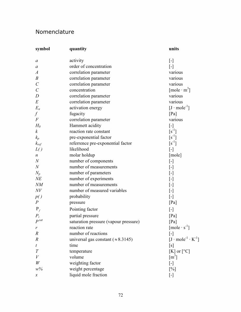
72

Nomenclature

symbol quantity units

a activity [-]

a order of concentration [-]

A correlation parameter various

B correlation parameter various

C correlation parameter various

C concentration [mole · m3]

D correlation parameter various

E correlation parameter various

Ea activation energy [J · mole-1]

f fugacity [Pa]

F correlation parameter various

H0 Hammett acidity [-]

k reaction rate constant [s-1]

kp pre-exponential factor [s-1]

kref referrence pre-exponential factor [s-1]

L( ) likelihood [-]

n molar holdup [mole]

N number of components [-]

N number of measurements [-]

Np number of parameters [-]

NE number of experiments [-]

NM number of measurements [-]

NV number of measured variables [-]

p( ) probability [-]

P pressure [Pa]

fΡ Pointing factor [-]

Pi partial pressure [Pa]

P sat

saturation pressure (vapour pressure) [Pa]

r reaction rate [mole · s-1]

R number of reactions [-]

R universal gas constant (≈8.3145) [J · mole-1 · K

-1]

t time [s]

T temperature [K] or [°C]

V volume [m3]

W weighting factor [-]

w% weight percentage [%]

x liquid mole fraction [-]

73

y vapour mole fraction [-]

z predicted model response [-]

z~ measured response [-]

Greek

ε absolute tolerance [-] γ activity coefficient [-] γ heteroscedasticity parameter [-]

φ fugacity coefficient [-]

µ chemical potential [J] µ mean [-]

υ stoichiometric factor [-]

nυ molar specific volume [m3 · mole

-1]

θ set of model parameters [-]

ξ measurement error [-]

π pi constant (≈3.1416) [-]

σ standard deviation [-]

Φ gPROMS objective function value [-]

ω heteroscedasticity parameter, standard deviation [-]

superscripts

+ protonated

0 reference state

sat saturated

´ unobservable parameter due to Bodenstein approximation.

´´ unobservable parameter in combination with available data.

subscripts

L liquid

L lower

U upper

V vapour

T total

74

indices

0 reference state (P = P sat)

i ith component

j jth reaction

k kth measurement

abbreviations

ACM Aspen Custom Modeler

CAPE Computer Aided Process Engineering

CO CAPE-OPEN

COSE CAPE-OPEN compliant Simulation Environment

CPU Central Processing Unit

CSTR Continuous Stirred Tank Reactor

FatnessDBI Fatness Dissolved Butenes Included

FO Foreign Object

GB Giga Byte

gPROMS general Process Modelling System

HCFA HydroCarbon Free Acid

LSQ Least Squares

MEK Methyl Ethyl Ketone

MLL Maximal log likelihood

NM Nelder-Mead

NRTL Non-Random Two Liquids

PP Property Package

PS Property System

PSE Process Systems Enterprise

RAM Random Access Memory

SBA Secondary-Butyl Alcohol

SED Sequential Experiment Design

SQP Sequential Quadratic Programming

VLE Vapour-Liquid Equilibrium

75

Appendix A Chemical structures of components

H H

O

H2O H2SO4

O

O

HO OH S CH2

CH

CH3

CH3

OH

SBA

MBS

CH2

CH

CH3

CH3

O

O

O OH S

CH2

CH +

CH3

CH3

C4+

SBE

CH2

CH

CH3

CH3

O

CH3

CH2

CH

CH3

H +

H +

N2

N

N

1-C4

H

C

CH2

H

H CH3

C

c2-C4

H

C

CH3

H

C

CH3

t2-C4

H

C

CH3 H

C

CH3

76

Appendix B Hammett acidity

In reactions involving the protonation of a weak base (butylenes in this case) by a strong

acid such as the 72% sulphuric acid used in the SBA process, the catalytic efficiency of

the acid is not a linear function of the acid concentration present in the reaction medium.

A measure of the ability of the acid to donate a proton to a weak base is given by the

Hammett acidity function. Experiments have been performed to obtain a correlation for

the Hammett acidity H0 as a function of two other variables: HCFA and FatnessDBI. The

Hammett acidity correlation is presented in equation (B.1).

2438

0 1071408.41035172.3 HCFAHCFAH ⋅⋅+⋅⋅=− −− 312 107997.31023125.5 FatnessDBIHCFA ⋅⋅−⋅⋅+ −− (B.1)

42162.06003.377132.1 2 −⋅−⋅+ FatnessDBIFatnessDBI

The variables ‘hydrocarbon free acid’ (HCFA) and the ‘Fatness dissolved butenes

included’ (FatnessDBI) are both a function of the liquid weight percentage of some of the

components as presented in (B.2) and (B.3) respectively. HCFA (Hydrocarbon-Free

Acidity) is a measure for the capability of the liquid to absorb hydrocarbons. The

mathematical expression for HCFA is

%100

213.1330

015.18%

123.74

015.18%%

182.154

074.98%%

182.154

074.98%%

,,,,4,

,4,

22

2

SBELSBALOHLMBSLSOHL

MBSLSOHL

wwwww

ww

HCFA

++++

+=

(B.2)

FatnessDBI is defined as the number of moles of C4 equivalents, including the dissolved

butane and butene isomers, per mole of H2SO4 equivalent present in the acid phase. The

mathematical expression for FatnessDBI is

182.154

%

074.98

%231.130

%2

123.74

%

108.56

%%%

182.154

%

,4,

,,2,2,1,,

2

444

MBSLSOHL

SBELSBALCtLCcLCLMBSL

ww

wwwwww

FatnessDBI

+

++++

+=

−−−

(B.3)

77

Samenvatting

De kinitiek parameters behorend bij het relevante reactieschema zijn vereist om een

chemische proces te optimaliseren dat plaatsvindt in de Sec-Butyl-Alcohol stripper die

bedreven wordt door Shell in Pernis. Hiervoor zijn in het verleden

laboratoriumexperimenten uitgevoerd, die gemodelleerd zijn met Aspen Custom Modeler

(ACM), een commercieel software pakket dat ontwikkeld wordt door AspenTech. Het

doel van dit afstudeerproject is de parameterschatting capaciteiten het softwarepakket

gPROMS, dat ontwikkeld wordt door Process Systems Enterprise, te beoordelen en te

vergelijken met die van ACM. Hiertoe dient een model van de laboratoriumexperimenten

ontwikkeld te worden met de gPROMS software dat zo equivalent mogelijk dient te zijn

aan het bestaande model in ACM. Daartoe zijn de fysische en thermodynamische

eigenschappen van de componenten in het ACM model beschikbaar gemaakt voor het

gPROMS model via de CAPE-OPEN interface, die succesvol toegepast is. Het model van

de experimenten dat ontwikkeld is in gPROMS bevat een vloeistof-damp evenwicht dat

de verdeling van negen componenten over beide fasen beschrijft die zeer goed

overeenkomt met het ACM model. Tijdens parameterschatten werd duidelijk dat niet alle

kinitiek parameters individueel waarneembaar zijn in combinatie met de beschikbare data

van de laboratoriumexperimenten. Het systeem is gedeeltelijk ge-herparameteriseerd en

de nieuwe set parameters is vervolgens bepaald met voldoende nauwkeurigheid.

Verschillende aspecten van parameterschatten met beide software pakketten zijn

behandeld, onder andere: invoer van experiment data, interpretatie van de uitvoer,

beschikbare combinaties van doelfuncties en optimalisatie methoden alsmede het

vermogen, de snelheid en de nauwkeurigheid van het verkrijgen van een oplossing van

deze combinaties. Aan de hand van de beoordeling van deze aspecten is geconcludeerd

dat de parameterschatting capaciteiten van gPROMS beter zijn dan die van ACM.

Vervolgens is onderzocht welk type experimenten vereist zijn om de kinetiek parameters

te schatten die niet waarneembaar zijn met de tot dan toe beschikbare data. Pogingen om

de gPROMS “Sequential Experiment Design” (SED) functionaliteit toe te passen waren

zonder succes, waardoor geen uitspraak gedaan kan worden over de toegevoegde waarde

van deze functionaliteit. Alternatief ontworpen experimenten zijn gesimuleerd met het

model dat bekende parameters bevat, vervolgens wordt de synthetische data gebruikt

voor het schatten van de parameters. Het effect van datareductie op de waarneembaarheid

van de parameters is tevens onderzocht. Er is gebleken dat het mogelijk is alle parameters

te schatten van drie reactie systemen met een gereduceerde set synthetische data.

Assessment of the parameter estimation capabilities of gPROMS ...

Documents

Transcript of Assessment of the parameter estimation capabilities of gPROMS ...