
Assessment Of The Channel Catfish Fishery In Saginaw · PDF fileASSESSMENT OF THE CHANNEL...
82
1 9 0 8 Assessment Of The Channel Catfish Fishery In Saginaw Bay, Lake Huron Robert M. Lorantas December 22, 1982
Transcript of Assessment Of The Channel Catfish Fishery In Saginaw · PDF fileASSESSMENT OF THE CHANNEL...

1 9 0 8
Assessment Of The Channel Catfish Fishery
In Saginaw Bay, Lake Huron
Robert M. Lorantas
December 22, 1982

MICHIGAN DEPARTMENT OF NATURAL RESOURCES FISHERIES DIVISION
Fisheries Research Report No. 1908
December 22, 1982
ASSESSMENT OF THE CHANNEL CATFISH FISHERY IN SAGINAW BAY, LAKE HURON 1
Robert M. Lorantas
This 1s a reprint of a thesis fulfillment of the requirements for Science in Fisheries, in the School The University of Michigan, 1983.
submitted in partial the degree of Master of of Natural Resources,
1 Contribution from Dingle-Johnson Study F-35-R, Michigan.

ASSESSMENT OF THE CHANNEL CATFISH FISHERY
IN SAGINAW BAY, LAKE HURON
by
Robert M. Lorantas
A thesis submitted in partial fulfillment of
the requirements for the degree of
Master of Science
in Fisheries
School of Natural Resources
The University of Michigan
1983
Thesis Committee:
Adjunct Professor William C. Latta, Chairman Assistant Professor James S. Diana Ex-officio examiner Richard D. Clark, Jr.

For Justin, Nell
and Kathy
l l l

ACKNOWLEDGEMENTS
Financial support for this project was provided by
the Institute for Fisheries Research of the Michigan
Department of Natural Resources (MDNR} and the School of
Natural Resources at the University of Michigan. It was
challenging and enjoyable to become a part of a great
institution and great school. The abilities and expertise
of my committee members provided my greatest inspiration as
an aspiring professional. I would first like to thank my
chairman, Dr. w. Carl Latta, for providing me with the
opportunity and encouragement to engage in this study. I
would also like to thank Dr. James S. Diana for his interest
and encouragement. Thanks are extended to Mr. Richard
D. Clark, Jr., of the MDNR, for allowing me to utilize a
number of programs he developed, and for the generous
assistance and encouragement he provided. The critical
reviews and support of all committee members contributed
significantly to this study. My appreciation is extended to
Dr. Karl F. Lagler, his unfailing enthusiasm as my graduate
advisor made graduate work enjoyable. Indeed all of my
professors contributed to the progress of this research, and
I thank them.
Numerous persons contributed to the development of
this project. Mr. Forrest Williams, Mr. Todd Williams,
Mr. Dennis Root, Mr. Richard Manor, and Mr. Samuel Morgan
supplied vessel time for sample collection. Mr. Ed Dootz
iv

provided laboratory space in the Dental Materials Department
at the University of Michigan. Mr. Andrew Nuhfer, Mr. Don
Nelson, Mr. Gale Jamson, and Mr. John Weber all of the MDNR
provided commercial and sportfishing catch data along with
useful information concerning the fisheries of Saginaw Bay.
Mr. Paul Haack, of the Great Lakes Fishery Laboratory of the
U. S. Fish and Wildlife Service, provided historical
commercial catch records. Fellow student, Tim Hill,
assisted in data collection. Many not mentioned here also
contributed. I thank everyone for their interest, kindness,
and time. Lastly, I extend my heartfelt thanks to my
parents and sister for their special support and
encouragement which allowed me to pursue my life long
interests.
V

ABSTRACT
Channel catfish Ictalurus punctatus ranked second in
weight harvested by commercial fishermen (231,000 kg), and
third in number caught by sportfishermen (60,000) in Saginaw
Bay in 1981. The commercial fishery employs trap nets,
seines, and set hooks. Mean annual catch per unit effort
for all gear types has increased in the past decade, in
comparison to prior decades, and has lead commercial
fishermen to request licensing of additional gear. The
commercial fishery was assessed using a dynamic pool model,
and an extension of the model was used to investigate the
dynamics of gear competition. Growth and total mortality
parameters, estimated from four management areas, were
pooled for model analysis since no significant differences
in these vital statistics were detected after the age of
complete recruitment to the fishery. Parameters of the
von Bertalanffy growth equation were estimated using mean
back-calculated lengths at age derived from fin spine
sections. Total instantaneous mortality was estimated from
the slope of the descending limb of a catch curve. Fishing
mortalities for each commercial gear type and for
sportfishing gear were estimated by partitioning the total
fishing mortality in proportion to the catch from that gear.
Pooling all areas yielded a von Bertalanffy equation of the
form Lx = 921(1-e(-o.o 9(x-o. 35 >>), and a total instantaneous
mortality of 0.67. Model predictions indicated that yield
Vl

to the commercial fishery and to the sport fishery could be
increased by increasing the minimum commercial size limit
and/or reducing the commercial fishing mortality.
Simulations also indicated that an increase in fishing
mortality by any one gear type increased yield to that gear
type, but reduced yield to all other gear types. The
tenuous nature of the estimates of sportfishing mortality
and natural mortality preclude specific management
recommendations.
vii

TABLE OF CONTENTS
DEDICATION ...
ACKNOWLEDGEMENTS •
ABSTRACT . . •
LIST OF TABLES .
LIST OF FIGURES
LIST OF APPENDICES .
INTRODUCTION .
BACKGROUND. . . . . METHODS . . . . . . . . . .
Data Collection ....... . Fin Spine Preparation ••..•.••..•• Back-calculation Using Fin Spines •. Age Composition and Size Structure of the Catch. Growth in Length . . . • . . Weight-Length Relation •.•• Mor ta 1 i ty . . . . . • . . . . . . . . Yield Analysis ....
RESULTS
Age Composition and Size Structure of the Catch. Growth in Length . Weight-Length Relation •...••.•••• Mortality .•.•••• Yield . . . . . . . . . . . . . . .
DISCUSSION
iii
iv
vi
ix
X
xi
3
9
9 9
10 13 13 15 15 20
23
23 25 27 29 29
44
Age Composition and Size Structure of the Catch. 44 Growth in Length . • . • . . . . 45 Weight-Length Relation . . . . 49 Total Mortality Rate . • . 49 Fishing Mortality Rates . . . • . • • • . . . . • 51 Yield • . . . . . . . . . • . • 54
LITERATURE CITED •. 60
Vlll

LIST OF TABLES
Table
1. Mean annual catch per unit effort for trap nets, seines, and set hooks and mean annual yield for all commercial gear types combined
Page
during selected time periods. • . • • • • • • 8
2. Sampling dates, number of lifts sampled, average trap net pot height, pot stretch mesh size, number of specimens sampled for total length measurement, and number of specimens subsampled for weight, spine removal, and sex from each grid in 1981. • . • • . . • • . • • 10
3. Mean back-calculated lengths-at-age derived from the the posterior and anterior fields of spine sections from the distal end of the basal recess, mean empirical lengths-at-age, and number of specimens aged in grid 1608. • • 12
4. Annual mail survey estimates of sport harvest of ictalurids (in number), fraction of channel catfish in the commercial harvest (in number), and adjusted estimate of yield (in weight) of sport-harvested channel catfish in Saginaw Bay ( 1975-1981). . . • • • . • • • • • • • • • • • 19
5. Estimated age distributions of channel catfish caught in commercial trap nets for each grid sampled and for all grids pooled. • • • 23
6. Yield to each gear type, fraction of total yield attributable to each gear type, and estimate of the instantaneous fishing mortalities due to each gear type in 1981. 31
7. Range of FS + M values used to examine the sensitivity of yield per 1000 recruits as a function of FC, and range of FS + M (and FC) values used to examine the sensitivity of yield per 1000 recruits as a function of le. • 39
8. Mean back-calculated lengths at age of channel catfish from Saginaw Bay in 1981 and 1971, and from other selected locations. • • • • • . • • 48
9. Instantaneous total mortality rates estimated for Saginaw Bay in 1981 and 1971, and for other selected locations. • . • • • . • . . • 52
lX

Figure
1.
LIST OF FIGURES
Map of Saginaw Bay, Lake Huron, the grid system used in sampling.
illustrating
2. Annual catch, effort and catch per unit effort for trap nets, seines, and set hooks from 1929
Page
5
to 1981.......... . . . . . . . . 6
3. Length frequency polygon of channel catfish caught in commercial trap nets for all grids pooled . . . . . . . . . . . . . . . . 24
4. Estimated von Bertalanffy growth curve and empirical mean back-calculated lengths at age with 95% confidence limits. • . • • . • • 28
5. Catch curve with regression line fitted to the descending limb (grids combined). • . • • 30
6. Yield isopleths per 1000 recruits as a function of FC and xc, with M=0.1 and FS=0.06. 32
7. Yield per 1000 recruits as a function of FC with FS=0.06, M=0.1, and 1 =381 mm; and for a range of FS + M values, with lc=381 mm. • • • 34
8. Yield per 1000 recruits to sport gear, seines, set hooks, and trap nets as a function of FR, where FS=0.06, FE=0.05, FH=0.14, M=0.1, and 1 c = 3 8 1 mm . • • . • • • . • • • • • . • 3 6
9. Yield per 1000 recruits to sport gear, seines, set hooks, and trap nets as a function of FH where FS=0.06, FE=0.05, FR=0.32, M=0.1, and lc=381 mm............... 37
10. Yield per 1000 recruits to sport gear, seines, set hooks, and trap nets as a function of FE where FS=0.06, FH=0.14, FR=0.32, M=0.1, and lc=381 mm. . . . . . . . . . . . . . . . • 38
11. Yield per 1000 recruits to the commercial fishery and sport fishery as a function of 1 where FS=0.06, FC=0.51, and M=0.1 ..•••. ~ 41
12. Yield per 1000 recruits as a function of 1 with FC=0.51, FS=0.06, and M=0.1; and for a range of FS + M values, with FC=0.51. . . • • 42
X

LIST OF APPENDICES
Appendix
A. Mean back calculated lengths at age for both sexes in each grid and for sexes combined. (Sample size and 95% confidence interval are
Page
indicated for each length.) • . . . • 66
B. Polynomials fitted to back-calculated lengths at all ages for each sex in each grid and for sexes pooled within grids. (Sample sizes and coefficients of determination are indicated.) 68
C. Linearized weight-length regressions for each sex in each grid, for sexes pooled within grids, and for sexes and grids pooled. (Sample sizes and coefficients of determination are indicated.) • • • • . • . . . . • • . . . . • 69
D. Equations fitted to the descending limbs of catch curves.for each grid and grids combined. (Sample sizes and coefficients of determination are indicated.) . • • . . . . . 70
Xl
INTRODUCTION
Channel catfish Ictalurus punctatus in Saginaw Bay,
Lake Huron, support both commercial fishing and
sportfishing. In 1981, sportfishermen harvested an
estimated 29,000 kg and commercial fishermen a reported
231,000 kg. Channel catfish are a valuable segment of the
commercial fishery and ranked second in weight harvested in
1981; common carp Cyprinus carpio ranked first (314,000 kg),
and yellow perch Perea flavescens ranked third (80,000 kg).
Yellow perch ranked first in number of fish harvested by
sportfishermen, sunfish species ranked second (these
included mostly bluegills Lepomis machrochirus and
pumpkinseeds k:._ gibbosus), and channel catfish ranked third.
It appears that there exists sufficient social and economic
impetus for the continued coexistence of recreational and
commercial fisheries throughout the Great Lakes. However,
allocation of fishery resources to their respective users
has been a difficult problem to solve (Francis et al. 1979;
Bishop and Samples 1980; Talhelm 1979). In the existing
fishing regime, the assessment of changes in yield or effort
levels of sport and commercial fisheries becomes even more
crucial to resource managers if yields acceptable to both
users are to be maintained.
Efforts to quantitatively evaluate multiple use of a
common fishery resource are limited (Clark and Huang 1983;
Low 1982). Yet, managing only the commercial fishery

2
without regard to the sport fishery or vice versa may be
futile in achieving a desired management objective.
Although sportfishing harvest records provide only an index
of the harvest of channel catfish in Saginaw Bay, available
records were utilized in this assessment. The objectives of
this study were: (1) to examine the history of sport and
commercial fisheries along with their regulation, (2) to
collect timely information concerning growth and mortality
rates of channel catfish in different areas of Saginaw Bay,
(3) to determine whether these vital statistics differ
between areas, and (4) to evaluate some management
strategies using available information in a
yield-per-recruit model.

3
BACKGROUND
Beeton et al. (1967) described the location,
morphometry, and limnological aspects of Saginaw Bay. Hile
(1959) described the multi-species and multi-gear character
of the fisheries in Saginaw Bay and documented changes in
species composition and gear composition utilizing
commercial catch records. The Great Lakes Basin Commission
(1975} summarized historical changes in sport and commercial
fisheries as well as associated changes in water chemistry
and aquatic biota and provided a broad perspective of the
dynamic nature of the Bay. Characteristics and regulation
of the commercial and sport fisheries for channel catfish
make them unique among fisheries of the Great Lakes. The
commercial fishery employs three major gear types: trap
nets, seines, and set hooks. Trap nets harvest all
commercially available species in the Bay, seines primarily
harvest common carp and channel catfish, and set hooks
harvest channel catfish exclusively. The contribution of
channel catfish in weight to the commercial harvest in 1981
was 63% for trap nets, 9% for seines, and 28% for set hooks.
All units of gear are licensed by the state; the type and
amount of gear licensed have evolved through restrictions
imposed by the state and by fishermen utilization of the
various gear types. In 1981, 400 trap nets, 16 seines, and
39,400 set
Additional
hooks were licensed to 28 commercial operators.
units of gear have not been available for

4
licensing since 1970 in areas of the Bay open to commercial
fishing (Great Lakes Fishery Commission 1971a).
Commercially fishable areas of the Bay have been largely
confined to the Inner Bay, that area southwest of a line
connecting Sand Point and Point Lookout (Fig. 1). Minimum
size and weight restrictions relating to commercial harvest
of channel catfish date from at least 1895 during which a
0.45 kg (1.0 lb) minimum weight limit was in effect. This
limit evolved into a 0.91 kg (2.0 lb) minimum weight limit
in 1929, a 432 mm (17 inch) minimum size limit in 1945, and
a 381 mm (15 inch) minimum size limit in 1960. The latter
regulation remains in effect. There are no season
restrictions governing commercial harvest.
Records of the annual commercial harvest of channel
catfish date from 1919 (Baldwin et al. 1979). Since 1929,
trap nets have accounted for the bulk of the commercial
catch, except during the period 1959 - 1965 when set hooks
produced the largest yields. Seines ranked second in weight
harvested until about 1956 and have since accounted for the
lowest yields. Change in effort was the apparent cause of
fluctuation in yield to each gear until the mid 1960's
(Fig. 2, A and B). Historically, the fishery has been
uncharacteristically stable among the commercially important
fisheries of the Bay (Hile 1959). Although catch, effort,
and catch per unit effort (CPUE) fluctuated from very low to
very high levels between 1940 and 1970, Eshenroder and Haas
(1974) concluded that these changes were not indicative of

5
SAND POINT
SAGINAW BAY LAI<£ HURON
Figure 1. Map of Saginaw Bay, Lake Huron, illustrating the grid system used in sampling.

6
ci'''''?"------------------------------------------------------------· A K. -
1111 1141 IHI IHI 1171 YEAR
Jo ... ------------------------------------------------------------.. TIAP NETS LIFTS X 1,000 SEINE HAULS X 100 _____ _
,,.,: .!4.C!!.!'. ~!IH~. ~.!4.~C:IS~P. !'. ti!! 20
10
. .. . . : .
. . . . . . . . . . .
'
·. ·. : .. •,
B
.. .. . . . . .. . ...
... ,,,---' , .................... ..., .......................... _. ................ ._ .................. """"' __ """' ............. """" 1121 1111 1141 IHI
YEAR IHI 1171
,, ... ------------------------------------------------------------~ tD: 0 ~ JO &.i tz :, 20 D: w D..
::C 10 u ~ u
TltAP NETS (KG/LIFT) C SEINES (KOLHAULl X to _____ _
,,.,: .!4.C!!.!'.S. !~!1/.'!l!rt -~~~~.!'.~l!l ~- !!
'"""~ .............. """" ............................................... _. ........ .__. ......... ----....... --..... 1121 1111 1141 IHI 1111 1171
YEAR
Figure 2. Annual catch, effort and catch per unit effort for trap nets, seines, and set hooks from 1929 to 1981. (See Hile (1962) for specific descriptions of effort units.)

7
significant changes or trends in population abundance
(Fig. 2). The Great Lakes Basin Commission (1975), however,
postulated that the downward trend in catch during the mid
1960's was probably due to a decline in abundance, since at
this time the value per pound was increasing. The decline
in catch, effort, and CPUE during the mid 1960's may,
likewise be associated with fear of mercury contamination
evident in catfish from other areas of the Great Lakes
during that era (Great Lakes Fishery Commission 1971b). The
mean annual catch in the period from 1970 to 1981 has
increased; this increase has been associated with an
increase in the mean annual CPUE for all gear types (Table
1). Thus, in contrast to the previous decade, these changes
are probably indicative of an increase in abundance. The
increases in CPUE have prompted requests by commercial
fishermen for the licensing of additional gear (John Weber,
Michigan Department of Natural Resources, personal
communication). A goal of this assessment was to determine
whether expenditure of additional commercial effort, perhaps
through the licensing of additional commercial gear, was an
appropriate management alternative.
Sportfishing has been found to have significant
impacts on fisheries exploited both commercially and by
sportfishermen (McHugh 1980). Sportfishing demand for
channel catfish has not been assessed in Michigan. However,
since 1975, estimates of the sport harvest of catfish of all
species have been made by the Michigan Department of Natural
8
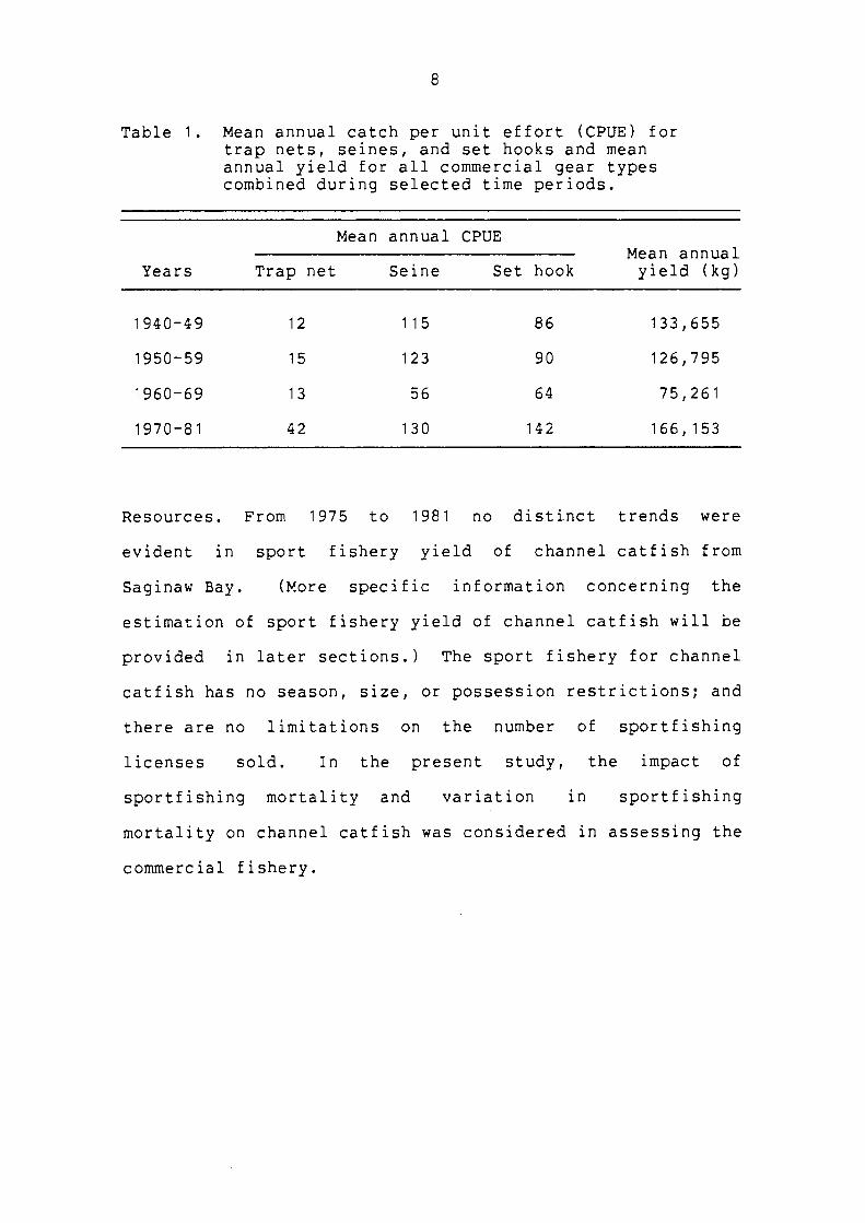
Table 1. Mean annual catch per unit effort (CPUE) for trap nets, seines, and set hooks and mean annual yield for all commercial gear types combined during selected time periods.
Mean annual CPUE Mean annual
Years Trap net Seine Set hook yield (kg)
1940-49 12 115 86 133,655
1950-59 15 123 90 126,795
1960-69 13 56 64 75,261
1970-81 42 130 142 166,153
Resources. From 1975 to 1981 no distinct trends were
evident in sport fishery yield of channel catfish from
Saginaw Bay. (More specific information concerning the
estimation of sport fishery yield of channel catfish will be
provided in later sections.) The sport fishery for channel
catfish has no season, size, or possession restrictions; and
there are no limitations on the number of sportfishing
licenses sold. In the present study, the impact of
sportfishing mortality and variation in sportfishing
mortality on channel catfish was considered in assessing the
commercial fishery.

9
METHODS
Data Collection
To estimate parameters which describe the growth and
mortality of channel catfish, commercial trap net catches
were sampled in each of four management areas (in grids
1608, 1509, 1507, and 1606) within the Inner Bay (Fig. 1).
The total length of all channel catfish from
catch was recorded to the nearest millimeter.
of approximately 10 to 20 specimens per 25 mm
a trap net
A subsample
group were
collected for further analysis. These fish were weighed to
the nearest gram using a spring scale, dissected to
determine sex, and the left pectoral spine was removed for
growth analysis. Sampling dates, the number of lifts
sampled, characteristics of the commercial sampling gear,
number of specimens collected, and number of specimens
subsampled from each grid are listed in Table 2.
Fin Spine Preparation
Specimens were aged from annuli observed on sections
of pectoral fin spines (Sneed 1951). Use of pectoral fin
spine sections for age determination of channel catfish has
been validated with known age specimens by Sneed (1951),
Marzolf (1955), and Prentice and Whiteside (1974). Spines
were removed as described by Sneed (1951), air dried, and
sectioned at the distal end of the basal recess. The
thickness of a section was determined by the thickness of a
spacer between two cutting discs similar to the method of

10
Table 2. Sampling dates, number of lifts sampled, average trap net pot height, pot stretch mesh size, number of specimens sampled for total length measurement, and number of specimens subsampled for weight, spine removal, and sex from each grid in 1981. When a pot consisted of two mesh sizes the size comprising the lesser area of the pot is listed in parenthesis.
Number Number Mean Pot Number of
of pot mesh of specimens lifts height size lengths sub-
Grid Month/day sampled (m) (mm) sampled sampled
1608 5/16-6/13 2 3.05 6.35 (4.44) 1051 264
1509 6/2-6/20 4 3.05 6.35 (4.44) 740 2 1 1
1507 7/16-8/4 18 1. 07 4.76 (5.17) 640 206
1606 8/1 6 2. 13 4.76 542 236
Chugunova (1959). I used aluminum oxide cutting discs and a
0.52 mm spacer rotated at 2750 RPM with a dental lathe. A
stream of water directed on the discs served as a lubricant
and coolant. After sawing, sections were air dried, and
then mounted on cellulose acetate slides with viscous
cyanoacrylate adhesive. Spine sections prepared in this
manner could be viewed with transmitted light using a scale
projector. Sections too thick for light transmission could
be made thinner with a fine toothed file.
Back-calculation Using Fin Spines
Back-calculated lengths were computed using the
formula described by Everhart and Youngs (1981). Several
problems have been encountered in calculating lengths using

1 1
spine sections. Muncy (1959) and Marzolf (1955) identified
the following causes of bias:
(1) Pectoral spines are tapered, and sections obtained at the basal recess, which expands distally with increasing age, decrease in relative size with increasing age.
(2) The maximum expanded portion of annuli in the commonly measured posterior field does not always lie in a straight line along the maximum radius.
(3) The center of the lumen of the spine, commonly used as the origin in making radial measurements to annuli, does not always correspond to the center of the first annulus.
(4) Spine sections are not always sectioned precisely perpendicularly.
DeRoth (1965) addressed the first problem by
sectioning spines at the same relative location. However, I
had diff~culty in consistently determining the appropriate
point of sectioning. DeRoth's method also produced sections
without a lumen or complete first annulus, making radial
measurement difficult. To counter both the first and the
second problems, Marzolf (1955) recommended measurement of
the anterior radius, which he suggested was less affected by
spine taper. To check this assumption I computed intercepts
(correction factors) and mean back-calculated lengths at age
for specimens from grid 1608 for both posterior and anterior
fields of spines sectioned at the distal end of the basal
recess. Total length was regressed on each spine radius; a
straight line adequately described these relationships. The
intercepts estimated for the anterior and posterior fields
were -46.1 and -198.7, respectively. The anterior radius

12
Table 3. Mean back-calculated lengths (mm) at age derived from the posterior and anterior fields of spine sections from the basal recess, mean empirical lengths (mm) at age, and number of specimens aged in grid 1608.
Age
2 3 4 5 6 7 8 9 10 11 12
Calculated posterior -100 1 1 140 237 300 350 410 460 499 542 580 597
Calculated anterior 51 129 196 254 307 353 413 460 500 542 582 597
Empirical 144 228 255 316 340 398 479 505 539 589 597
Number of specimens 0 2 28 46 9 3 12 24 9
produced calculated lengths similar to empirical lengths at
age, while the posterior radius produced calculated lengths
which were negative and erroneous (Table 3).
The degree to which the third and fourth problems
affect the analysis depends upon how carefully spines are
measured and sectioned. I took the following precautions to
mitigate or eliminate all the previously described problems:
(1) The anterior radius was measured which alleviated problems associated with spine taper at the basal recess.
( 2) Annuli in the anterior field were concentric with respect to the center of the first annulus of the section. Therefore, measurement along this field reduced the error associated with measurement of expanded annuli in the posterior field.
(3) The approximate center of the first annulus was used as the or1g1n for radial measurement which decreased error associated with use of an irregularly positioned or irregularly shaped lumen.

13
(4) Spines were marked prior to sectioning which facilitated cutting perpendicular sections and reduced mechanical difficulties associated with positioning the spine during the sectioning process.
Age Composition and Size Structure of the Catch
Age distributions of catches were estimated using
age-length keys (Allen 1966). Age-length keys were
constructed for each grid sampled and applied to the length
distribution of the catch from that grid. This procedure
afforded independent estimation of the age distribution of
the catch from each grid, and thus avoided possible bias due
to age composition differences among grids (Kimmura 1977).
Estimated age distributions from each grid were then
compared with a G-test (Sokal and Rohlf 1981). The computer
program, CHITAB, facilitated computation of the attained
significance level for the G-test (Statistical Research
Laboratory 1976). A length-frequency polygon of the
combined catch of all grids was also constructed to
determine the size of complete recruitment to the trap net
fishery.
Growth in Length
Total length was regressed on anterior spine radius
for each sex in each grid using least squares. A straight
line adequately described these relationships. The
intercepts of the regression equations were compared between
sexes and grids. Data were pooled for grids and sexes with

14
similar intercepts and a common intercept (correction
factor) was used to compute back-calculated lengths. Back-
calculated lengths were used to check for growth differences
which would preclude use of an average growth function to
describe growth of each sex and growth in each of the four
management areas of the Bay. Although the von Bertalanffy
function is appropriate for and was fitted to the
length-at-age data in this study, interpretations of the
parameters of this function for comparative purposes and
statistical tests concerning these parameters have been
controversial (Gallucci and Quinn 1979; Kingsley et
al. 1980). To statistically compare growth, back-calculated
lengths were regressed on age for both sexes in each grid.
Visual inspection of the relationship between back-
calculated length and age, and residual analysis indicated
that a second degree polynomial adequately described this
relationship.
where
y = back-calculated length in mm;
X = age in years;
BO = intercept;
B1 = linear effect coefficient;
B2 = curvature effect coefficient.
Regression equations and regression parameters were compared
to test for growth differences. Linear and curvature effect
coefficients, which describe the shape of the length-age

15
relations, were compared between regression equations to
check for differences in growth rate. If differences did
not exist, intercepts were compared to check for differences
in the magnitude of lengths-at-age.
Weight-Length Relation
The weight-length relation, w = alb, was linearized
with a natural log transformation:
where
w = weight in kg;
1 = length in mm;
loge(a) = intercept;
b = slope.
The natural log of weight was regressed on the natural log
of length for each sex in each grid, and the equality of
these regression equations was tested. All weight-length
data were later pooled to estimate an average weight-length
relation for use in yield calculations.
Mortality
The total instantaneous mortality rate (Z) was
estimated for each grid sampled by determining the slope of
a straight line fitted to the descending limb of a catch
curve (Ricker 1975). Everhart and Youngs (1981) recommended
fitting the regression line to age groups which include the
age group 1 year older than the modal age group and extend
to the age group 1 year younger than the oldest age group

captured.
bias due
16
These recommendations were intended to reduce
to gear selectivity and small sample variation.
Catch curves in this study, however, exhibited considerable
variability. Variability near the domes did not permit
accurate determination of the first fully recruited age
group, therefore in fitting regression lines to the
descending limbs, the modal age group was assumed to be
fully recruited. The oldest age group was also assumed to
be appropriately represented and was used in calculating the
slope of the descending limb. Instantaneous total mortality
rates were compared by testing for differences in the slope
parameters of the regression equations.
All regression parameters, test statistics, and
attained significance levels were computed using MIDAS, a
computer program for data analysis developed by the
Statistical Research Laboratory at the University of
Michigan (Fox and Guire 1976). All statistical tests were
based upon a 5% level of significance.
The total instantaneous fishing mortality rate (FT)
was estimated by subtracting the instantaneous natural
mortality rate (M) from the instantaneous total mortality
rate (Z):
FT= Z - M.
I could not estimate the natural mortality rate from my
data, so I used the rate of 0.1 reported by Eshenroder and
Haas (1974). The instantaneous fishing mortality for each
gear type or fishery was estimated by multiplying the total

17
instantaneous fishing mortality by the proportion of yield
attributable to each gear or fishery for 1981. Partitioning
forces of fishing mortality in this manner assumes that
these competing risks of capture are independent, and thus
additive. Therefore,
FT= FS +FR+ FE+ FH,
where
FT = instantaneous total fishing mortality;
FS = instantaneous sportfishing mortality;
FR = instantaneous trap net fishing mortality;
FE = instantaneous seine fishing mortality;
FH = instantaneous set hook fishing mortality.
The Michigan Department of Natural Resources annually
compiles the weight of fish harvested by each commercial
gear type from reports submitted by commercial fishermen,
and annually conducts a mail survey to estimate numbers of
fish harvested by sportfishermen. Several adjustments of
the mail survey data had to be made to make this information
suitable for my use. First, the survey estimated the
combined harvest of all ictalurids 2 from Saginaw Bay. To
estimate the sport harvest of channel catfish alone, I
assumed the fraction of channel catfish in the combined
commercial harvest was the same as in the sport harvest.
(The weight harvested commercially was available to the
2 Ictalurus spp. in Saginaw Bay includes nebulosus, the brown bullhead; natalis, the yellow bullhead; and punctatus, the channel catfish.

species
reported
level.) Second,
in numbers of
18
sport
fish
harvest estimates were
harvested, while commercial
harvest was reported in weight. Thus, I had to estimate the
average weights of fish harvested in the respective
fisheries to get harvest in common units of measure. Using
pooled weight and length data from this study I calculated
the average weight of a channel catfish in the commercial
catch to be 1.0 kg, 2.2 lb (fish~ 381 mm, 15 inches in
length), and the average weight of a sport-harvested fish to
be 0.4 kg (0.9 lb) (assumed to be the average weight of fish
~ 299 mm, 12 inches, in length). The average weight of a
bullhead species was assumed to be 0.2 kg (0.4 lb), as
reported for brown bullheads by Blumer (1982). Finally,
Rybicki and Keller (1978) reported that mail survey
estimates were inflated for some species by factors of 5 to
20. Overestimation of harvest by a factor of 5 has been
substantiated by other research and is used as a standard
correction for mail survey estimates of catch for most
species in Michigan (Talhelm et al. 1979). Thus, as a
final adjustment, I reduced estimates of sport harvest in
weight of channel catfish to one-fifth of their estimated
values. Putting all these adjustments together it was
possible to estimate the weight of channel catfish harvested
by sportfishermen (Table 4). The 1981 sport harvest
estimate and reported commercial harvest by gear type were
then used to partition FT.
19
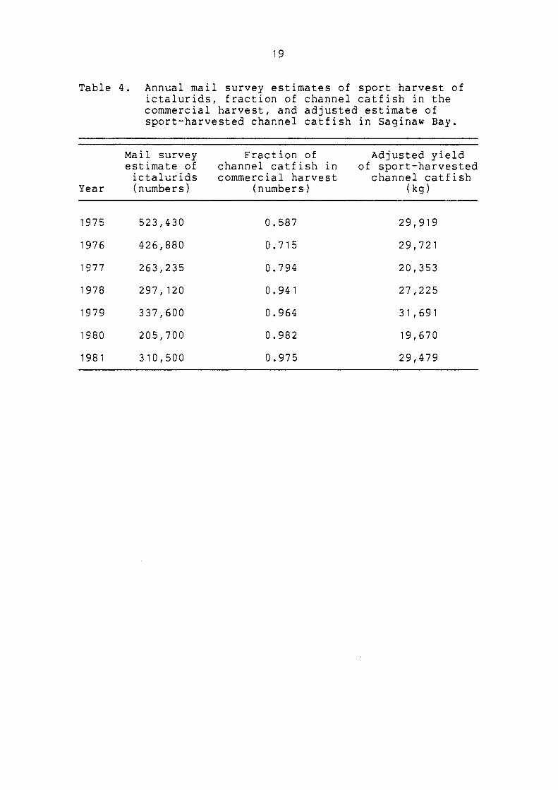
Table 4. Annual mail survey estimates of sport harvest of ictalurids, fraction of channel catfish in the commercial harvest, and adjusted estimate of sport-harvested channel catfish in Saginaw Bay.
Mail survey Fraction of Adjusted yield estimate of channel catfish in of sport-harvested ictalurids commercial harvest channel catfish
Year (numbers) (numbers) (kg)
1975 523,430 0.587 29,919
1976 426,880 0.715 29,721
1977 263,235 0.794 20,353
1978 297,120 0.941 27,225
1979 337,600 0.964 31,691
1980 205,700 0.982 19,670
1981 310,500 0.975 29,479

20
Yield Analysis
An idealized view of the dynamics of a catfish
fishery could be described schematically as follows:
Recruitment Population
Growth Biomass
Natural Mortality Trap net Mortality Set hook Mortality Seine Mortality Sport Fishing Mortality
Additions to the population come in the form of growth and
recruitment and losses arise from natural, trap net, seine,
set hook, and sportfishing mortality. This approach is an
extension of the cohort-yield approach of Beverton and Holt
(1957) and Ricker (1975), and accounts for fishing mortality
from four independent sources rather than one. The model I
used, developed by R. D. Clark, Jr. of the Michigan
Department of Natural Resources, was parameterized so that
it accommodated four independent sources of fishing
mortality. The model was used to calculate the yield per
number of fish recruited (N) at the age of first
vulnerability to fishing (xr). (In all analyses the number
of fish recruited at age xr was set at 1000.) From age xr
to the age at which fish were harvested (xc), losses were
assigned to natural mortality. When fish reached an age (x)
greater than xc, losses were assigned both to natural
mortality and fishing mortality due to all gear types (FT):

21
dN/dx = -MN x s;xs;x r C
dN/dx = -(FT+M)N x>x • C
Catch rate was then described in terms of each gear type
x>x • C
Integrating and combining these equations resulted in a
catch equation where the number of fish at each age caught
by each gear (cx,g> was:
where
Zx = (FT+M)[(x+1)-x].
The von Bertalanffy equation of growth in length was used to
calculate mean length at age and the weight-length relation
was used to estimate the mean weight at age. Mean weights
at age multiplied by the mean number harvested at age for
each gear produced the weight harvested at each age by each
gear. Summing the weights harvested at all ages for each
individual gear type produced the yield in weight by gear
per 1000 recruits.
The model utilized length at capture (le) and length
at recruitment (lr) data which were converted to age at
capture (xc) and age at recruitment (xr). The length at
recruitment (lr) to all gear types was defined to be the
mean length of fish less than or equal to the modal length
of fish in the length frequency distribution of the
commercial catch. This length was also assumed to be the

22
size acceptable to sportfishermen. A more detailed
mathematical description of a similar model is presented in
Clark and Huang (1983).
Yield to the commercial fishery per 1000 recruits was
sensitive to changes in FS and M. These parameters were
combined (FS + M) to examine this sensitivity. Yield to the
commercial fishery per 1000 recruits was examined for FS + M
values of: 0.1, 0.16, 0.2, 0.25, 0.3, 0.35, 0.4, and 0.45.
Yield-per-recruit analyses were performed in conjunction
with various commercial minimum size limit regimes and
commercial fishing mortality regimes to identify conditions
under which maximum yield occurred. Only changes in
regulation of the commercial fishery were considered,
however the implications of these changes were evaluated for
both sport and commercial fisheries.

23
RESULTS
Age Composition and Size Structure of the Catch
Estimated age distributions of channel catfish caught
in commercial trap nets were significantly different between
grids (G-test, P<0.01). The modal age of fish captured in
grids 1509 and 1608 was age 6, in grid 1507 age 7, and in
grid 1606 age 5. In grids 1608 and 1606, a greater
proportion of individuals less than age 6 were captured than
in grids 1509 and 1507 (Table 5). Differences in catch
characteristics were probably associated with differences in
availability of channel catfish at the time of sampling, and
differences in the selective properties of the sampling
gear. With all ages pooled, age 6 was the modal age
captured (Table 5), and 340 mm (13 inches} was the modal
length of channel catfish captured (Fig. 3).
Table 5. Estimated age distributions of channel catfish caught in commercial trap nets for each grid sampled and for all grids pooled.
Age
Grid 2 3 4 5 6 7 8 9 10 11 12 13
1608 0 0.1 0.6 8.6 2.5 69.0 4.7 1.6 4.2 7.0 1.2 0.5 0
1509 0
1507 0
0
0
0
0
5.0 0.7 60.4 12.7 2.4 5.9 8.7 2.7 1.4 0.1
1.0 9.5 12.7 56.4 9.5 1.1 4.6 3.6 1.3 0.3
1606 0 0.6 5.7 17.5 38.7 4.6 22.0 3.3 1.3 3.0 2.2 1.1 0
All O 0.1 1.2 7.7 10.2 43.1 20.9 3.8 3.4 6.2 2.3 1.0 0.1

24
0.35
z 0,30 0
~ 0 z
0.25 >-0 z LaJ ::> 0.20 0 LaJ Q:: Y.. LaJ 0.15 > ~ ...J LaJ Q::
0.10
0.05
o.oo-t-..... --.----.... ----.~--...-----.~--...---~ .. --.... __ --~ 100 180 260 340 420 500 580 660 740 820
LENGTH INTERVAL MIDPOINT {MM)
Figure 3. Length frequency polygon of channel catfish caught in commercial trap nets for all grids pooled (interval width= 40.0 mm).

25
Growth in Length
Length-age regressions were significantly different
between sexes and grids (f-test, P<0.0001). To identify
where these differences occurred, regressions between sexes
within grids were compared. These regressions were not
significantly different in grids 1507 (f-test, P=0.82) and
1606 (f-test, P=0.57), but were significantly different in
grids 1509 (f-test, P<0.0001) and 1608 (f-test, P=0.0003).
There were significant differences between shape parameters
(B 1 s and B2 1 s) in grids 1509 (f-test, P<0.0001) and 1608
(f-test, P=0.0001) which indicated that differences in
growth rate existed between males and females in these
grids. Mean back-calculated lengths at age were greater for
females after age 6 in grid 1608 and greater for males at
all ages in grid 1509 (Appendix A). These conflicting
growth differences were probably due to differential
vulnerability of the sexes to capture during the spawning
season rather than real growth differences. Although
statistically significant differences in growth rate existed
between sexes in grids 1509 and 1608, sexes were pooled to
check for spatial growth differences.
With sexes pooled length-age regressions were
significantly different between grids (f-test, P<0.0001).
The shape parameters of the regression equations were not
significantly different (f-test, P=0.06), however the
intercepts (B 0 1 s) were significantly different (f-test,
P<0.0001). Pairwise comparisons indicated that regression

26
equations were identical in grids 1507 and 1509 (f-test,
P=0.89). The intercepts of the length-age regressions in
grids 1608 and 1606 were less than the intercepts in grids
1509 and 1507 (Appendix B). In grid 1608, mean back
calculated lengths at age were less from age 1 to age 9 than
in other grids (Appendix A). These differences were
probably associated with differences in vulnerability of
various size classes to capture during the spawning season.
In grid 1606, mean back-calculated lengths at age were less
than those in grids 1507 and 1509 (Appendix A). These
differences were probably associated with differences in
availability of various size classes, as well as differences
in selective properties of the sampling gear. A regression
equation fitted to back-calculated lengths versus age after
age 6, the age of complete recruitment to the fishing gear,
indicated that the length-age relation was the same between
all grids (f-test, P=0.3). Differences in length-at-age did
not appear great enough to treat growth between sexes or
management areas separately, therefore growth was described
by a single function in the yield-per-recruit analysis. The
von Bertalanffy function was fitted to the mean back-
calculated lengths at age, for grids and sexes pooled, using
the method of Rafail (1973). The equation derived was:
L = 921 ( 1-e(-0.09(x-0.35))), X

27
where
Lx = length at age x (mm);
x = age in years.
The model agreed quite closely with the empirical data
(Fig. 4).
Weight-Length Relation
Weight-length regressions between sexes and grids
were significantly different (f-test, P<0.0001). To
identify where these differences occurred, regressions
between sexes within grids were compared. Regressions
between sexes were not significantly different [1608 (f
test, P=0.34), 1509 (f-test, P=0.10), 1507 (f-test, P=0.10),
and 1606 (f-test, P=0.10)].
equations were significantly
test, P<0.0001). Differences
probably reflect differences
However, with sexes pooled
different between grids (f
in weight-length equations
in condition associated with
the time of year the
Pooling all grids
samples were collected (Table 2).
and sexes yielded the following weight-
length relation used to compute mean weight from mean length
in yield calculations:
Regression equations for each sex within each grid and for
sexes pooled within grids are listed in Appendix C.

28
100...---------------------------------------------......
700
600 Lx = 921(1-e{-0.09{x-0.35)})
~ 500
:::E ~ ~
:c: 400 ~ (.!) z Lu ...J
300
200
100
0 ..... --........... ----------------..-------------.---.--............ 0 2 3 4 5 6 7 8 9 10 11 12 13 14
AGE (YEARS)
Figure 4. Estimated von Bertalanffy growth curve and empirical mean back-calculated lengths at age with 95% confidence limits.

29
Mortality
Total instantaneous mortality rates and 95%
confidence intervals for grids 1608, 1509, 1507, and 1606
were 0.57 (±0.53), 0.63 (±0.36), 0.66 (±0.48), and
0.45 (±0.30), respectively. The slopes of the descending
limbs of the catch curves were not significantly different
between grids (f-test, P=0.79). Combining age frequencies
reduced some variability in the descending limb of the catch
curve, however considerable variability remained (Fig. 5).
The total instantaneous mortality rate (Z) and 95%
confidence interval for all grids pooled was 0.67 (±0.27).
(Regression equations fitted to catch curves are listed in
Appendix D.) Thus, the instantaneous fishing mortality rate
was 0.57, (0.67 less the natural mortality of 0.1). This
rate was partitioned in proportion to the yield to each gear
type to obtain an estimate of the instantaneous fishing
mortality rate for each gear type (Table 6). Using this
information the instantaneous commercial fishing mortality
rate was 0.51 and defined as:
FC =FR+ FH + FE.
Yield
Similarities in the growth and mortality rates of
channel catfish from each management area in Saginaw Bay
indicated that fish from the entire Bay comprised a unit
stock for the purposes of a yield-per-recruit analysis
(Gulland 1969). Parameters estimated from pooled growth and
mortality data were used in yield computations. Using the

30
a.....-------------------------------------------....
7 p-,
I \
I \ Y = 11.0-0.67(X} I \
I 9 R2 = 0.86
6 I
I \
I \ \
fl \ I \ /""°,
5 I \ I ' / \
:::c I q \
0 I ' d \
~ _.,,
I \
'b 0 4
I ' I ' Q) I ' (!) , ' 0 I \ ....J I 3 I
I I
I I
2 I I
I d
0-,..--.,...--...... ...,,.... ...... --.... --..... --...---..-~,.... ... --.... --------1 2 3 5 6 7 8 9 10 11 12 13 U
AGE(YEARS)
Figure 5. Catch curve with regression line fitted to the descending limb (grids combined).

31
Table 6. Yield to each gear type, fraction of total yield attributable to each gear type, and estimates of the instantaneous fishing mortalities due to each gear type in 1981.
Fraction of Yield total Instantaneous
Gear (kg) yield fishing mortality
Trap nets 146,626 0.563 0.32
Set hooks 63,481 0.244 0. 14
Seines· 20,809 0.080 0.05
Sport gear 29,479 0.113 0.06
Total 260,395 1. 00 0.57
best estimate of sportfishing mortality (0.06) and natural
mortality (0.1), yield to the commercial fishery per 1000
recruits was examined as a function of the instantaneous
commercial fishing mortality (FC) and the age at entry to
the fishery (xc), or commercial minimum size limit (le).
Model predictions indicated that yield per 1000 recruits
could be increased by increasing xc and/or decreasing FC
from their existing or estimated values of 381 mm
(15 inches) and 0.51, respectively (point Qin Fig. 6). The
largest gains in commercial yield could be realized by
increasing le.
One approach to evaluate the effects of changes in FC
and le upon commercial yield was to examine each of these
parameters independently as a function of yield per 1000
recruits. At the existing or estimated values of FS (0.06),

32
22 789.8
20 400 KG 763.9 -V) a:: 18 732.9 <( 500 KG LaJ >- -'.J 16 ::IE 695.8 ::E LaJ
600 KG -a:: I-:::> ::IE ~ 14 650 KG 651.4 a.. ...I
<( a..,
0 N
~ 12 598.2 en
V) _ - EUMETRIC LINE - - - - - - - - ::IE
a:: -- ~
--- ::IE ,. La.. 10
,,, 534.6 ~ ,,
~ / ::IE
/ I
LaJ 8 458.3 (!) <( I
I
6 367.1
4 257 .9 0.0 0.5 1.0 1.5 2.0 COMMERCIAL INSTANTANEOUS FISHING MORTALITY
Figure 6. Yield isopleths per 1000 recruits as a function of FC and x (corresponding values of 1 are indicated), w!th M=0.1 and FS=0.06. c The commercial fishery was operating at point Qin 1981 •
33
M (0.1), and le (381mm, 15 inches) model predictions
indicated that the maximum commercial yield per 1000
recruits occurred when the value of FC was approximately
0.20 (Fig. 7). Thus, at the estimated FC value of 0.51 the
commercial fishery was growth overfishing (Cushing 1981).
Model predictions indicated that a decrease in FC from 0.51
to 0.20 produced a 5.7% increase in equilibrium yield per
1000 recruits to the commercial fishery and a 117.6%
increase in equilibrium yield per 1000 recruits to the sport
fishery. Commercial fishing mortality could be reduced by
reducing the total amount of fishing gear licensed on the
Bay, further restricting areas of the Bay open to commercial
fishing, restricting the length of the fishing season,
imposing taxes, and in other ways (Clark 1976).
To evaluate the implications of gear requests by
commercial fishermen only changes in the total amount of
gear licensed were considered. Thus, an increase or
decrease in FC would be controlled by increasing or
decreasing the amount of gear licensed. Using this
management framework, a change in FC could be accomplished
in two ways: (1) by proportionally changing the fishing
mortality caused by all commercial gears, or (2) by
selectively changing the fishing mortality caused by any
combination of commercial gear types or any one gear type.
Proportional changes in the instantaneous fishing mortality
caused by each commercial gear type would not change the
distribution of catch among gear types. However, selective

34
900...------------------------------------------------
100
s ~ 700
Cl) 1--::, 600 Q: u L&J Q:
0 0 0 .....
500
Q: -400 L&J £L
C _J 300 L&J
>-200
100
I I
I I I I I I I I I I I I I
' \ \
\ \
' ' ' ' ' ' ' ... ... ... ...... ... .... 0.1 _ -- --- --- ------; ... ------- 0.16 ________ _.J : .," ------0.20------------------• ,' I / ... ----------- Q.25------------------1 I ".,, I I .1 ---------·0.30------------------1 I ......
I I .,... 0 35 ------------------:: / .," ...... --------- 0"40------------------
1 I I.I "" ... .- - - - - - - - - - - 0 • 45 - - - - - - - - - - - - - - - - - -,, , / ,,, ... ---------- . II .I ., ...
I " .- .-I/ I ..I .,, ,, , .,., ..1" ,,,,.,., ,,, ., u,
O-t--.1m1m11,.....--,...,. .. ...,..,...,.....,. ..... ..,. ..... .,....,._.._ .. ...,_...,._. 0 0.5 1 1.5 2
COMMERCIAL INSTANTANEOUS FISHING MORTALITY
Figure 7. Yield per 1000 recruits as a function of FC with FS=0.06, M=0.1, and 1 =381 mm (solid line): and for a range of FS + M cvalues, with lc=381 mm (broken lines).

35
changes in fishing mortalities due to each gear type would
alter the distribution of catch among each gear type. For
simplicity, the change in yield per 1000 recruits was
examined for each gear type as a function of the
instantaneous fishing mortality caused by only one
commercial gear type. A reduction in fishing mortality of a
single commercial gear type reduced the yield to that gear
type and increased yield to other gear types. Conversely,
increases in fishing mortality of a single commercial gear
type increased the yield to that gear and reduced yield to
other gear types (Figs. 8, 9, and 10). Any net reduction in
commercial fishing mortality increased yield to
sportfisheirnen.
Considering the commercial fishery as a whole, the
value of FC which produced the maximum yield per 1000
recruits increased as values of FS + M increased (Fig. 7).
Therefore, errors in the estimates of FS, M, or both; or
changes in the values of FS, M, or both could affect the
conclusions derived from this analysis. I examined the
potential consequences of these problems by analyzing the
relation of FC to commercial yield per 1000 recruits for a
range of FS + M values (Table 7). For each FS + M value
examined a total instantaneous mortality rate of 0.67 was
maintained by adjusting the estimate of FC so that:
FS + M + FC = 0.67.

36
200
100
0 o.o 0.5 1.0 1.5 2.0
200
100 SEINES -(!) 0 ~ ._,, 0.0 0.5 1.0 1.5 2.0 en ~ 400 ::, £t: u 300 La.I £t:
0 SET HOOKS 0 200
0 9-
£t: 100 La.I Q..
C 0 ....J La.I o.o 0.5 1.0 1.5 2.0 >-
400
300
200
100
0 o.o 0.5 1.0 1.5 2.0
TRAP NET INSTANTANEOUS FISHING MORTALITY
Figure 8. Yield per 1000 recruits to sport gear, seines, set hooks, and trap nets as a function of FR, where FS=0.06, FE=0.06, FH=0.14, M=0.1, and lc=381 mm.

37
200
100
0 0.0 0.5 1.0 1.5 2.0
200
100· SEINES
///////,fl I I I - 0 C, I ' • ~ o.o 0.5 1.0 1.5 2.0
Cl) 400 .... -:::,
0:: 300 0 ..... 0:: 0 200 0 0 100 .... 0:: .....
0 0..
0 o.o 0.5 1.0 1.5 2.0 ...J ..... 500 >
400
300 TRAP NETS
200
100
0 o.o 0.5 1.0 1.5 2.0
SET HOOK INSTANTANEOUS FISHING MORTALITY
Figure 9. Yield per 1000 recruits to sport gear, seines, set hooks, and trap nets as a function of FH where FS=0.06, FE=0.05, FR=0.32, M=0.1, and lc=381 mm. ·

38
200..--------------------------------------------.
0.5 1.0 1.5 2.0
400
300
.-... (!) 200 0 V)
100 t--:::> 0::
~ 0 0:: o.o 0.5 1.0 1.5 2.0
0 200 0
0 ..... 0:: 100 LaJ Q.
Q 0 ...J LaJ o.o 0.5 1.0 1.5 2.0 ->-
400
300
200 TRAP NETS
100
0 o.o 0.5 1.0 1.5 2.0
SEINE INSTANTANEOUS FISHl~G MORTALITY
Figure 10. Yield per 1000 recruits to sport gear, seines, set hooks, and trap nets as a functi~n of FE where FS=0.06, FH=0.14, FR=0.32, M=0.1, and lc=381 mm.
39
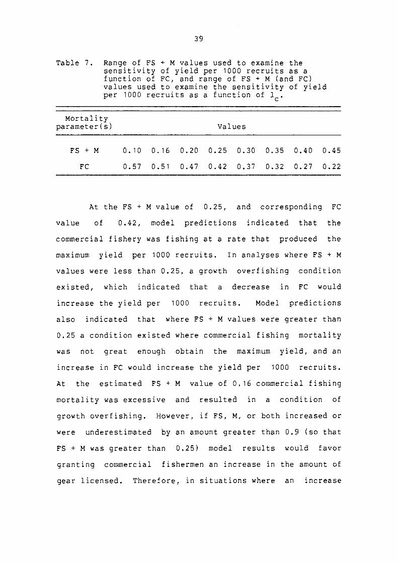
Table 7. Range of FS + M values used to examine the sensitivity of yield per 1000 recruits as a function of FC, and range of FS + M (and FC) values used to examine the sensitivity of yield per 1000 recruits as a function of le.
Mortality parameter(s)
FS + M
FC
Values
0.10 0.16 0.20 0.25 0.30 0.35 0.40 0.45
0.57 0.51 0.47 0.42 0.37 0.32 0.27 0.22
At the FS + M value of 0.25, and corresponding FC
value of 0.42, model predictions indicated that the
commercial fishery was fishing at a rate that produced the
maximum yield per 1000 recruits. In analyses where FS + M
values were less than 0.25, a growth overfishing condition
existed, which indicated that a decrease in FC would
increase the yield per 1000 recruits. Model predictions
also indicated that where FS + M values were greater than
0.25 a condition existed where commercial fishing mortality
was not great enough obtain the maximum yield, and an
increase in FC would increase the yield per 1000 recruits.
At the estimated FS + M value of 0.16 commercial fishing
mortality was excessive and resulted in a condition of
growth overfishing. However, if FS, M, or both increased or
were underestimated by an amount greater than 0.9 (so that
FS + M was greater than 0.25) model results would favor
granting commercial fishermen an increase in the amount of
gear licensed. Therefore, in situations where an increase
40
in FC is being considered the importance of accurately
estimating and monitoring changes in FS and Mis clearly
demonstrated.
At the existing or estimated values of FC (0.51), FS
(0.06), and M (0.1), model predictions indicated that the
maximum commercial yield per 1000 recruits occurred when le
was approximately 550 mm, 22 inches (Fig. 11). Increasing le
from 381 mm (15 inches) to 550 mm (22 inches) produced a
28.8% increase in equilibrium yield per 1000 recruits to the
commercial fishery and a 171.6% increase i.n equilibrium
yield per 1000 recruits to the sport fishery. Increases in
le up to 550 mm (22 inches) resulted in increases in yield
per 1000 recruits to both the sport fishery and commercial
fishery, however when le became greater than 550 mm
(22 inches),
(Fig. 11).
yield to the commercial fishery declined
The value of le, which produced the maximum yield per
1000 recruits, was also sensitive to changes in the value of
FS + M, and this sensitivity was examined for the range of
values presented in Table 7. At the FS + M value of 0.30,
and corresponding FC value of 0.37, model predictions
indicated that the current minimum commercial size limit of
381 mm (15 inches) produced the maximum yield per 1000
recruits (Fig. 12). In analyses where FS + M values were
less than 0.3, a condition existed where fish were harvested
at a size less than that which produced the maximum
commercial yield, which indicated that an increase in le

41
700
600
500
-400 SPORT F'ISHERY
300
200 s ~ 100 Cl) .... ::> 0 0:: 300 -400 500 600 700 800 0 LI.I 0::
0 0 0 - 800 0:: LI.I a.. 700 Q ..J 600 LI.I
>-500
-400
300
200
100
0 300 -400 500 600 700 800
COMMERCIAL MINIMUM SIZE LIMIT {MM)
Figure 11. Yield per 1000 recruits to the commercial fishery and sport fishery as a function of le where FS=0.06, FC=0.51, and M=0.1.

-C) ~ ..._, (I) ~
::) Ct: u L&J Ct:
0 0 0 -Ct: L&J 0...
C ...J L&J
>-
1300
1200
1100
1000
900
800
700
600
500
-400
300
200
100
42
0.16
.,,,,,,,,,. .... ------------ 0.20 ,,,,,,.,,,,,,. ',
..... ' ' ' ' '
------------- 0.25 ' ' ' '
.. .. ------------ ', - 0.30 ........... -------- -- 0.35 ...... .... .... ------ .... ........... ', ---- --o.4o ........ ,.... ,, --- --- .... .............. ', 0 ~5-- ... ... .... .. ....
' ' ' ' ' ' .... ---- --- ............. ,........ ', ---- ---- ............ ....__ ', --- --- -- ' ------- ---0-t---~,,_--.... ----.... --..... ,...--... ----..... --.... - ................... ~---... -....
300 -400 500 600 700 800 COMMERCIAL MINIMUM SIZE LIMIT (MM)
Figure 12. Yield per 1000 recruits as a function of 1~ with FC=0.51, FS=0.06, and M=0.1 (solid line), and for a range of FS + M values (brokery lines), with FC=0.51.

43
would increase the yield per 1000 recruits. Model
predictions also indicated that where FS + M values were
greater than 0.3 a condition existed where fish were
harvested at a size greater than that which produced the
maximum yield, and a decrease in le would increase the yield
per 1000 recruits. At the estimated FS + M value of 0.16, a
low commercial minimum size limit resulted in a condition of
growth overfishing. However, if either FS, M, or both were
were underestimated or increased by an amount greater than
0.14 (so that FS + M was greater than 0.3) model results
would favor a le of 381 mm (15 inches), or perhaps less.
Thus, accurately estimating and monitoring changes in FS and
Mis also important in situations where a change in le is
being considered.

44
DISCUSSION
Age Composition and Size Structure of the Catch
Estimated age distributions of the catch of channel
catfish were different in each grid sampled. Differences in
age distributions could be attributed to age-specific
differences in availability, age-specific differences in
vulnerability to the sampling gear, and real differences in
age composition between grids. Greater proportions of
younger age groups were captured in grids 1608 and 1606
(Table 5). Randolph and Clemens (1976) found that smaller
channel catfish occupied shallower water areas in culture
ponds, and larger channel catfish occupied deeper water
areas. Grids 1608 and 1606 are characterized by more
extensive shallow water areas, perhaps attractive to younger
age groups, and grids 1509 and 1507 are characterized by
more extensive deep water areas, perhaps attractive to older
age groups. This suggests that the observed differences in
age distributions were due to differences in availability of
various age groups. Although it appeared that younger age
groups were captured in proportion to their availability in
grids 1608 and 1606, even larger proportions were retained
in nets in grid 1606, which had smaller pot mesh than nets
in grids 1608, 1509, and 1507. This suggests that some age
specific differences in vulnerability to the fishing gear
also existed.

45
Growth in Length
There were significant differences in the growth rate
of channel catfish between sexes in grids 1509 and 1608.
Mean back-calculated lengths at age were greater for males
in grid 1509 and greater for females in grid 1608
(Appendix A). Few studies have compared growth in length of
channel catfish between sexes. Elrod (1974) and Ambrose and
Brown (1971) contended that growth in length between sexes
was similar enough in their studies to be combined. DeRoth
(1965) found that the average back-calculated lengths of
males and females in Lake Erie was similar up to age 4.
After age 4, mean back-calculated lengths at age were
greater for males. In experimental ponds, Beaver et
al. (1966) found that the average length of males was
greater than the average length of females. Thus, growth
differences between sexes in this study, in particular in
grid 1608, were more likely due to differential
vulnerability of males and females to capture rather than
real growth differences. Grids 1509 and 1608 were sampled
near the spawning season at a time when behavioral
differences have been observed between sexes. Trap nets are
passive sampling devices, and vulnerability to capture was
dependent upon movement. Larger channel catfish spawn
earlier in the spawning season, and males drive away females
and care for the eggs after spawning (Clemens and Sneed
1957). Thus, larger males may have been less vulnerable to
capture in grid 1608, if sampling took place early in the

46
spawning season when larger males were on their nests.
Also, hatching has been observed to take place after
approximately 1 week of incubation (Clemens and Sneed 1957).
If adult males disperse soon after the eggs hatch, it is
plausible that larger males were more vulnerable to capture
at this time. This may explain the larger back-calculated
lengths at age observed for males in grid 1509, although
growth differences evident in grid 1509 were consistent
with other reported results.
When sexes were pooled, no significant differences in
growth rate were detected between grids. However, mean
back-calculated lengths at age were less for channel catfish
from grids 1608 and 1606 than from other grids. These
differences may be real, may be associated with age-specific
differences in availability, or may be associated with net
selectivity. More younger fish were captured in grids 1608
and 1606 than in grids 1509 and 1507 (Table 5). In grid
1608, a greater proportion of smaller channel catfish may
have been captured, because larger fish, in particular
males, were probably on or near nests and less available at
the time of sampling. In grid 1606, the smaller pot mesh
utilized may have selected greater proportions of smaller
fish. Although mean back-calculated lengths at age were
smaller in grids 1608 and 1606 than in other grids, no
significant differences in growth rates or intercepts were
detected between grids when regression equations were fit to
47
lengths after age 6, the age of complete recruitment to the
commercial fishery.
Pooled mean back-calculated lengths at age in this
study were about average when compared to those reported
from other northern regions, and were smaller than those
reported from more southerly locations (Table 8). Mean
back-calculated lengths in this study were less than those
reported 10 years earlier by Eshenroder and Haas (1974). In
their study, channel catfish were captured with commercial
and experimental nets; experimental nets captured younger
age classes of channel catfish in greater proportion than
commercial gear types (Eshenroder and Haas 1974). I sampled
fish from commercial trap nets exclusively. If differences
in selectivity of the gear caused the observed growth
differences, one would expect fish in the present study to
be larger on the average at each age, since commercial nets
probably selected greater proportions of larger fish.
However, mean back-calculated lengths at age were greater in
the study conducted by Eshenroder and Haas (1974), thus,
gear selectivity probably did not account for the observed
growth differences.
Physical, chemical, and biological conditions have
been demonstrated to be quite dynamic in Saginaw Bay
(Rossman and Treese 1982), and these changes may explain the
observed differences in growth. Conditions which may have
caused a decrease in growth of channel catfish include:

Table 8. Mean back-calculated lengths (mm) at age of channel catfish from Saginaw Bay in 1981 (with 95% confidence intervals) and 1971, and from other selected locations.
Age Year(s) of Sample
Location study size 1 2 3 4 5 6 7 8 9 10 11 12 13 14
Saginaw Bay, Lake Huron 1981 916 54 132 198 256 310 358 420 469 507 546 594 604 612 ±1 ±2 ±2 ±2 ±3 ±3 ±5 ±6 ±6 ±8 ±14 ±20 ±76
Saginaw Bay, Lake Huron' 1 ' 1971 253 69 157 254 335 404 490 561 569 589 607 630
Lake Erie, Western Basin''' 1965 1,478 63 165 226 269 297 330 363
Lake Erie, Michigan Waters' 1 ' 1971 495 170 221 264 305 340 373 386 417 452 505 549
Lake St. Clair 1 1 1 1969-71 507 76 208 226 272 350 383 434 485 531 564 604
St. Lawrence River' ' ' 1975 28 119 164 204 239 272 302 330 353 377 400 432 455 """ 00
Lake Sharpe, South Dakota''' 1945-56 535 46 124 196 256 312 381 442 490 546 617 645 640 676
Ok 1 ahoma' ' ' 1946-54 7,717 101 215 302 368 409 452 504 555 607 630 644 648 655 731
Santee-Cooper Reservior System, South Carolina''' 1959 210 86 185 284 368 442 531 602 665 726 772 807 853 917 904
Farm Ponds, Central Texas' 1 • 1972 82 178 333 429 516 ... . . .
'I' Eshenroder and Haas ( 197 4)
DeRoth (1965)
'J' Maguin and Fradette (1975)
' . ' Elrod (1974)
' ' ' Jenkins ( 1954)
' 6 ' Stevens ( 1959)
'1' Prentice and Whiteside (1975)

(1) A decrease in primary productivity as demonstrated by a decrease in median chlorophyll a levels from 1974 to 1979 (International Joint Commission 1980).
(2) Intraspecific competition due to an increase in channel catfish abundance as demonstrated by the increases in catch per unit of effort (Fig. 2).
(3) Interspecific salmonid and programs.
competition due to intensified walleye Stizostedion vitreum stocking
Numerous other factors could contribute to the observed
decrease in mean length at age.
Weight-Length Relation
Differences in the linearized weight-length relations
between management areas probably reflect seasonal change in
weight and length (Bagenal 1978). Grids were not sampled
during the same time period and the slope of the relations
decreased from spring to summer (Appendix C). This
indicated that condition or plumpness decreased (Lagler
1956). Simco and Cross (1966) noted a similar decline in
condition of channel catfish in the late summer. Despite
these seasonal changes in condition, pooled weight and
length data were used in yield analyses to calculate the
approximate weight of the catch.
Total Mortality Rate
Ricker (1975) identified the following conditions or
assumptions implied in interpreting the descending right
limb of a catch curve:

50
(1) The age groups under study are equal in number when each is recruited to the fishery.
(2) Survival rate is uniform with age.
(3) Fishing and natural mortality rates are uniform with age, since both comprise the total mortality rate which is the complement of the survival rate.
(4) The sample is random.
Catch curves for each grid were characterized by
irregular right limbs which were probably caused by variable
recruitment. The right limbs exhibited the usual decreasing
trend with age and the variability appeared to be random.
Thus, I assumed that the slope of a line fitted by least
squares to the descending limb adequately estimated the
total instantaneous mortality rate. The irregularity of the
right limbs of the catch curves also precluded detection of
curvature, useful in evaluating the assumption of uniform
survival. However, commercial fishing effort information
provided insight to the constancy of survival, since
commercial fishing accounts for the bulk of total mortality.
Commercial fishing effort, and thus commercial fishing
mortality were relatively constant in years just prior to
1981, therefore survival rate was also probably constant
(Fig. 2, B).
The assumption of random sampling implies that
differences did not exist in age-specific vulnerability to
trap nets after the age of maximum vulnerability.
Differences in age structure of the catch were detected
between grids, however no differences in total mortality

51
were detected after the age of complete recruitment. This
indicated that differences in age composition were primarily
due to differences in availability or selectivity before the
age of complete recruitment to the fishing gear. Latta
(1959), and Laarman and Ryckman (1982) demonstrated that
trap nets were size selective for a number of species.
Ricker (1975) contended that error from catch curve
mortality estimates due to size-specific vulnerability was
unlikely to be large for trap nets, but encouraged efforts
to assess selectivity. Yeh (1977) showed that trap nets
were more effective in representing the length class
frequency of a population of channel catfish than gill nets
and hoop nets in large inland lakes in Texas. Assessment of
the selectivity of commercial trap nets for channel catfish
and collection of age frequency data over a series of years,
to minimize the effects of variable recruitment, would
enhance the reliability of the total mortality estimate.
The total instantaneous mortality rate for channel
catfish estimated in this study was identical to the value
estimated by Eshenroder and Haas (1974). This value also
lies within the range of other published values (Table 9).
Thus, it appears that the physical, chemical, and biological
changes that have occurred since the study by Eshenroder and
Haas (1974), have had little effect on total mortality.
Fishing Mortality Rates
The method used to estimate the instantaneous fishing
mortality rate for each gear or fishery was contingent upon

52
Table 9. Instantaneous total mortality rates estimated for Saginaw Bay in 1981 (with 95% confidence interval) and 1971, and for other selected locations.
Location
Saginaw Bay, Lake Huron
Saginaw Bay, Lake Huron< 1 >
Des Moines River, Iowa< 2 > ·
Upper Mississippi, Iowa< 3 >
Lake Sharpe, South Dakota< 4 >
Rivers of Sacramento Valley, Ca 1 i for n i a < s >
< 11 Eshenroder and Haas (1974)
<2 >Mayhew (1972)
< 3 >pitlo and Bonneau (1979)
c "'Elrod (1974)
c 5 >McCammon and LaFaunce (1961)
Year(s) of
study
1981
1971
1966-69
1977-79
1945-56
1955-59
z
0.67 (±0.27)
0.67
0.637
0.94
0.37
0.82
the reliability of the catch statistics used to partition
FT. Commercial records provided the catch for each gear
type as reported by commercial fishermen. These records
were assumed to be reliable. Sportfishing post card survey
estimates, however, have been demonstrated to be inflated,
and corrections for this have been described. These
correction factors were largely derived from exploitation
studies of lake trout Salvelinus namaycush and yellow perch.
Specific corrections for channel catfish would improve the

53
reliability of sport harvest estimates used here, and thus
improve the estimates of the instantaneous fishing rates for
each gear or fishery. A sportfishing mortality estimate of
approximately 0.20 would result if the estimate of
sportfishing yield were not corrected. Coupling this FS
value with the best estimate of M (0.1) yielded an FS + M
value of 0.30. Using this FS + M value model predictions
indicated that the commercial fishery was operating at a
minimum size limit and fishing rate very near that which
produced the maximum yield per 1000 recruits (Fig. 12).
Thus, results of the yield analysis greatly depend upon the
correction factor used in the estimation of sportfishermen
yield. An inaccurate correction factor could change the
conclusions drawn from this analysis.
Ultimately, the reliability of all of these fishing
mortality estimates depend upon the accuracy of the estimate
of FT. The indirect procedure used to estimate FT in
Saginaw Bay was exclusively dependent upon the estimate of z
and the value of M estimated by Eshenroder and Haas (1974).
The degree to which FT and M make up Z can significantly
influence yield computations. Model results indicated that
when natural mortality accounted for a larger percentage of
total mortality; maximum yield was obtained at greater
fishing rates (Fig. 7) and/or lower minimum size limits
(Fig. 12). Estimates of Mand FT from the Sacramento Valley
were 0.38 and 0.44, respectively (McCammon and LaFaunce
1961); each mortality parameter constituted approximately

54
one half of Z. In contrast, values from Saginaw Bay were
0.1 and 0.57 for M and FT, respectively. Here, the
instantaneous fishing mortality constituted a significantly
larger portion of Z, and model predictions indicated that
maximum yield was obtained at a relatively low fishing rate
and high minimum size limit. A more direct estimation
procedure to assess fishing and natural mortality (such as a
tag-recapture procedure) would ultimately be necessary to
improve estimates of natural and fishing mortalities and/or
validate the method used to estimate fishing mortalities.
Yield
Beverton and Holt (1957) listed the following
assumptions implied in a cohort yield-per-recruit model:
(1) Yields predicted are those which exist under equilibrium conditions.
(2) Extrapolation of model results to a population requires constant recruitment.
(3) Rates of growth and natural mortality remain constant in response to other changes.
(4) All fish older than age xr are equally vulnerable to capture.
Ricker (1975) identified the following assumptions
applicable to the competing gear types modeled in the
present study:
(5) The units of gear are distributed such that all fish are equally vulnerable to capture and there is no possibility of localized depletion of the stock.
(6) There is no physical interference among gear types with respect to their operation.

55
The utility of the results of this analysis depend to a
large degree, upon how well all of these assumptions were
met. With respect to the first assumption it is important
to recognize that predictions from this analysis in response
to a particular management action will not be realized
immediately. Lag time to attainment of a new equilibrium
will depend upon the management action, the generation time,
and recruitment (Walters 1969). For example, an increase in
the commercial minimum size limit would ultimately increase
yield, yet upon implementation a short-term reduction in
yield to the commercial fishery would result. Clark (1976)
discusses strategies which minimize these short term losses.
The impacts of management actions upon recruitment
cannot be assessed with this yield-per-recruit model.
Although recruitment has exhibited some variability, the
history of stab-le landings indicates that the assumption of
constant recruitment is probably appropriate for the current
total mortality rate and growth regime. However, fishing
mortality could become great enough to affect recruitment.
Russell (1942) documents some devastating consequences of
recruitment overfishing in the North Sea, and symptoms of
recruitment overfishing have been documented for channel
catfish in the Mississippi River (Pitlow and Bonneau 1979).
An understanding of the relation between stock and
recruitment would significantly enhance management
capability.

56
Changes in growth and natural mortality in response
to changes in management actions or environmental changes
have not been evaluated, yet model predictions hinge upon
the constancy of these vital statistics. Using the best
mortality and growth parameter estimates, model predictions
indicated that an increase in the minimum commercial size
limit and/or reduction in commercial fishing mortality would
increase both commercial and sportfishermen yield. Either
of these changes would ultimately change the relative
abundance of some age classes of channel catfish (Ricker
1975). These density changes could affect growth and
natural mortality. Model results indicated that small
changes in natural mortalfty significantly affected model
predictions (Figs. 7 and 12). However, the apparent
increase in abundance of channel catfish and changes in
environmental conditions, since the study by Eshenroder and
Haas (1974), have not resulted in any apparent changes in
natural mortality as evidenced by the constancy of total
mortality and fishing effort from 1971 to 1981. Growth,
however, may change in response to changing environmental
conditions or changes in density as a consequence of a
management action. The growth of channel catfish in Saginaw
Bay in 1971 and in Michigan waters of Lake Erie were used to
study model predictions under different growth regimes.
Mean back-calculated lengths at age of channel catfish in
Saginaw Bay in 1971 were greater than those in the present
study and mean lengths at age after age 6 were less in

57
Michigan waters of Lake Erie than in the present study
(Table 8). Using the 1971 growth regime in a yield analysis
similar to that performed in the present study, Eshenroder
and Haas (1974) concluded that an increase in the minimum
commercial size limit would increase yield. I concluded the
same using von Bertalanffy parameters fit to Lake Erie
growth data with the Saginaw Bay mortality regime. Thus, it
appears that small changes in growth that may occur 1n
response to a management action, or change in environmental
conditions, will not significantly affect model predictions.
The assumption of equal vulnerability to each gear
type was not directly assessed. Not all areas of Saginaw
Bay are commercially fishable, yet all areas are accessible
by sportfishermen. Each commercial gear type is suited to
exploit fish at a particular depth, on a particular bottom
type, and to some degree during a particular season. Thus,
all fish were probably not equally vulnerable to all gear
types. Since it appears that fishing does not result in
localized depletions of the stock, model bias due to
differences in vulnerability would probably be small.
However, a better understanding of the characteristics of
the catch from each gear would permit refinement of the
model and enhance predictions. The nature of the
distribution of the different types of fishing gear in time
and space indicates that physical competition between gear
types would be minimal.

58
Although the assumptions of the yield-per-recruit
model cannot be rigidly met, some useful management insights
can be gleaned from this study. First, examination of gear
competition
interesting.
in a realistic management framework was
With the best available growth and mortality
estimates, I determined that increases in commercial fishing
mortality through the licensing of additional gear, would
not increase yield to the fishery as a whole. Each
commercial gear type was operating at a level which produced
less than the maximum yield per 1000 recruits to that
particular gear (Figs. 8, 9, and 10), thus, yield to any one
gear type could be increased by increasing fishing mortality
due to that particular gear type. These increases, however
could only be realized with accompanying l~sses to other
gear types and a net loss to the fishery as a whole.
Second, yield-per-recruit analyses of the commercial fishery
indicated a condition of growth overfishing. This condition
could be corrected by increasing the minimum commercial size
limit, reducing the commercial fishing mortality, or a
combination of both. The largest gains in yield could be
obtained by increasing the minimum commercial size limit
(Fig. 6).
Increasing the minimum commercial size limit would
appear to benefit both the commercial and sport fishery.
Although all model results presented suggest that catfish
yield could be increase by increasing the commercial minimum
size limit, the tenuous nature of the mortality parameter

59
estimates precludes any immediate recommendation for a
change. However, efforts should be made to more accurately
estimate mortality parameters, and entry should remain
limited until these assessments are completed and specific
management plans can be formulated.

60
LITERATURE CITED
Allen, K. R. 1966. Determination age-length keys and length 7040 FORTRAN v. Transactions Society 95:230-231.
of age distribution from distributions, IBM 7090,
of the American Fisheries
Ambrose, J., Jr., and, B. E. Brown. 1971. Fecundity, age, growth, and condition of channel catfish in an Oklahoma reservoir. Proceedings of the Oklahoma Academy of Science 51:15-22.
Bagenal, T. 1978. Methods for assessment of fish production in fresh water, IPB Handbook No.3. Blackwell Scientific Publications, London, England.
Baldwin, N. s., R. w. Saafeld, M. A. Ross, and H. J. Buettner. 1979. Commercial fish production in the Great Lakes 1867-1977. Great Lakes Fishery Commission, Technical Report No. 3, Ann Arbor, Michigan, USA.
Beaver, J. A., K. E. Sneed, and H.K. Dupree. 1966. The difference in growth of male and female channel catfish in hatchery ponds. The Progressive Fish Culturist 28:47-50.
Beeton, A. M., S. H. Smith, and F. F. Hooper. 1967. Physical limnology of Saginaw Bay, Lake Huron. Great Lakes Fishery Commission Technical Report No. 12, Ann Arbor, Michigan, USA.
Beverton, R. J. H., and, of exploited fish Series 2, Volume Fisheries, and Food
S. J. Holt. 1957. On the dynamics populations. Fishery Investigation
19, Ministry of Agriculture, (Great Britain).
Bishop, R. c., and K. C. Samples. 1980. commercial fishing conflicts: a theoretical Journal of Environmental Economics and 7:220-233.
Sport and analysis.
Management
Blumer, L. S. 1982. Parental care and reproductive ecology of the North American catfish Ictalurus nebulosus. Doctoral dissertation. The University of Michigan, Ann Arbor, Michigan, USA.
Chugunova, N. I. 1959. Handbook for the study of age and growth of fishes. A~ademiya Nauk Press, Moscow, USSR. (English version 1963. Age and growth studies in fish. Office of Technical Services Washington, D. C., USA.)

61
Clark, C. w. 1976. Mathematical bioeconomics. Wiley Interscience, New York, New York, USA.
Clark, R. D., Jr., and B. Huang. 1982. The dynamics of competition between sport and commercial fishing: effects on rehabilitation of lake trout in Lake Michigan. Michigan Department of Natural Resources, Fisheries Research Report 1909, Ann Arbor, Michigan, USA.
Clemmens, H. P., and K. E. Sneed. 1957. The spawning behavior of the channel catfish Ictalurus punctatus. United States Department of the Interior Fish and Wildlife Service, Special Scientific Report No. 219. Washington, D.C. USA.
Cushing D. H. 1981. Fishery biology a study in population dynamics. The University of Wisconsin Press, Madison, Wisconsin, USA.
DeRoth, G. C. 1965. Age and catfish in western Lake Management 29:280-286.
growth Erie.
studies of channel Journal of Wildlife
Elrod J. H. 1974. Abundance, growth, survival, and maturation of channel catfish in Lake Sharpe, South Dakota. Transactions of the American Fisheries Society 103:53-58.
Eshenroder, R. L., and, R. C. Haas. 1974. Status of selected stocks in Lake Huron and recommendations for commercial harvest. Michigan Department of Natural Resources, Technical Report 73-32. Pages 105-206 in Bails, J. D., and M. H. Patriarche, editors. Status of Selected fish stocks in Michigan's Great Lakes waters and recommendations for commercial harvest. Michigan Department of Natural Resources, Fisheries Division, Lansing, Michigan, USA.
Everhart, W. H., and fishery science. York, USA.
W. D. Youngs. 1981. Principles of Cornell University Press, Ithaca, New
Fox, D. J., and K. E. Guire. 1976. Documentation for MIDAS 3rd edition. Statistical Research Laboratory, Ann Arbor, Michigan, USA.
Francis, G. R., J. J. Magnuson, and H. A. Regier. 1979. Rehabilitating Great Lakes ecosystems. Great Lakes Fishery Commission, Technical Report No. 37, Ann Arbor, Michigan, USA.

62
Gallucci, v. F., and T. J. Quinn II. 1979. Reparameterizing, fitting , and testing a simple growth model. Transactions of the American Fisheries Society 108:14-25.
Great Lakes Basin Commission. 1975. Great Lakes Basin Framework Study Appendix 8 Fish. Great Lakes Basin Commission, Ann Arbor, Michigan, USA.
Great Lakes Fishery Commission. 1971a. Minutes of Lake Huron Committee Meetings Appendix II. Great Lakes Fishery Commission, Ann Arbor, Michigan, USA.
Great Lakes Fishery Commission. 1971b. Minutes of Lake Erie Fishery Commission, Committee Meetings. Great Lakes
Ann Arbor, Michigan, USA.
Gulland, J. A. 1969. Manual of methods for fish stock assessment. Part 1. Fish population analysis. Food and Agriculture Organization of the United Nations Manuals in Fisheries Science 4, Rome, Italy.
Hile, R. 1959. Fluctuations in the Saginaw Bay 1885-1956. United Interior, United States Fish Research Report 51, Washington,
commercial fisheries of States Department of and Wildlife Service
D. C., USA.
Hile, R. 1962. Collection and fishery statistics in the Fishery Commission, Technical Michigan,
analysis of commercial Great Lakes. Great Lakes Report No. 5, Ann Arbor,
International Joint Commission. 1980. 1980 report on Great Lakes water quality. Toronto, Ontario, Canada.
Jenkins, R. M. 1954. Growth of channel catfish in Oklahoma waters: 1954 revision. Oklahoma Fisheries Research Laboratory Report 41, Norman, Oklahoma, USA.
Kimura, D. K. 1977. Statistical assessment of the agelength key. Journal of the Fisheries Research Board of Canada 34:317-324.
Kingsley, C. S., V. F. Gallucci, and T.J. Quinn II. 1980. Von Bertalanffy growth parameters. Transactions of the American Fisheries Society 109:252-253.
Laarman, P. w., and J. R. Ryckman. 1982. Relative size selectivity of trap nets for eight species of fish. North American Journal of Fisheries Management 2:33-37.
Lagler, K. F. 1956. Freshwater Fishery Biology. Wm. C. Brown Company, Dubique, Iowa, USA.

63
Latta, W. C. 1959. Significance of trap net selectivity in estimating fish population statistics. Papers of the Michigan Academy of Science, Arts, and Letters 44:123-138.
Low, R. A., Jr. 1982. Mortality rates and management strategies for black sea bass off the southeast coast. North American Journal of Fisheries Management 1:93-103.
Maguin, E., and G. Fradette. 1975. Growth of the channel catfish (Ictalurus punctatus) in the St. Lawrence River near Quebec. Journal of the Fisheries Research Board of Canada 32:1867-1870.
Marzolf, R. C. 1955. Use of pectoral spines and vertebrae for determining age and rate of growth of the channel catfish. Journal of Wildlife Management 19:243-249.
Mayhew, J. 1972. Some biological characteristics of a channel catfish population in the lower Des Moines River with an evaluation of potential commercial harvest. Iowas Conservation Commission Fisheries Section, Technical Series 72-2, Des Moines, Iowa, USA.
McCammon, G. w., and D. A. LaFaunce. 1961. Mortality rates and movement in the channel catfish population of the Sacramento Valley. California Fish and Game 47:5-26.
McHugh, J. L. 1980. Progress and problems in implementing the Fishery Conservation and Management Act of 1976. Transactions of the North American Wildlife and Natural Resources Conference 45:149-156.
Muncy, R. J. 1959. Age and growth of channel catfish from the Des Moines River, Boone County, Iowa, 1955 and 1956. Iowa State Journal of Science 34:127-137.
Pitlow J., Jr., and D. Bonneau. 1979. Assessment of change in commercial size limit of channel catfish. Iowa Conservation Commission Fisheries Section, Final Report Commercial Fisheries Investigations, Des Moines Iowa, USA.
Prentice, J. A., and B. G. Whiteside. 1974. Validation of aging techniques for largemouth bass and channel catfish in central Texas farm ponds. Proceedings of the Annual Conference Southeastern Association of Game and Fish Commissioners 28:414-428.
Rafail, S. z. 1973. A simple and precise method for fitting a von Bertalanffy growth curve. Marine Biology 19:354-358.

64
Randolph, K. w., and H. P. Clemens. 1976. Home areas and swimways in channel catfish culture ponds. Transactions of the American Fisheries Society 105:725-730.
Ricker, W. E. 1975. Computation and interpretation of biological statistics of fish populations. Fisheries Research Board of Canada Bulletin 191, Ottawa, Canada.
Rossmann, R., and T. Treese. 1982. Lake Huron bibliography with limited summaries. Great Lakes Research Division, Great Lakes and Marine Waters Center, The University of Michigan Special Report 88, Ann Arbor, Michigan, USA.
Russell, E. S. 1942. The overfishing problem. Cambridge University Press, London, England.
Rybicki, R w., and M. Keller. 1978. The lake trout resource in Michigan waters of Lake Michigan, 1970-1976. Michigan Department of Natural Resources, Fisheries Division, Fisheries Research Report No. 1863, Ann Arbor, Michigan, USA.
Simco, B. A., and F. B. Cross. 1966. Factors affecting growth and production of channel catfish Ictalurus punctatus. University of Kansas, Museum of Natural History 17:191-256.
Sneed, K. E. 1951. channel catfish, Transactions of 80:174-183.
A method for calculating growth of Ictalurus lacustris punctatus.
the American Fisheries Society
Sokal, R. R., and F. J. Rohlf. principles and practice of research 2nd edition. W. H. California, USA.
1981. Biometry: the statistics in biological
Freeman, San Francisco,
Statistical Research Laboratory. description. The University of Michigan, mimeo, 2p.
1976. CHITAB Michigan, Ann
general Arbor,
Stevens, R. E. 1959. The white and channel catfishes of the Santee-Cooper Reservoir and tailrace sanctuary. Proceedings of the Annual Conference Southeastern Association of Game and Fish Commissioners 13:203-219.
Talhelm, D. R., R. C. Bishop, K. W. Cox, W. Smith, D. N. Steinnes, and A. L. w. Tuomi. 1979. Current estimates of Great Lakes fisheries values: 1979 status report. Great Lakes Fishery Commission, Ann Arbor, Michigan, rnimeo report 79-1:17p.

65
Talhelm, D.R. 1979. Fisheries: dollars and cents. Water Spectrum 11:8-16.
Walters, C. J. 1969. A generalized computer simulation model for fish population studies. Transactions of the American Fisheries Society 98:505-512.
Yeh, C. F. 1977. Relatively selectivity of fishing gear used in a large reservoir in Texas. Transactions of the American Fisheries Society 106:309-313.

66
APPENDIX A.
Mean back-calculated lengths at age for both sexes in each grid and for sexes combined.

Table A-1. Mean back-calculated lengths (mm) at age for both sexes in each grid and for sexes combined. (Sample size and 95% confidence interval are indicated for each length. Sex was not determined for all specimens, therefore the sample sizes of males and females may not sum to the combined sample size.)
Age
Grid 1 2 3 4 5 6 7 8 9 10 11 12 13
Male 47 126 193 254 308 356 409 452 489 533 572 533 ±3 ±4 ±4 ±5 ±7 ±7 ±10 ±14 ±16 ±22 ±61
(135) (135) (135) (133) (105) (104) (58) (49) (46) (34) ( 10) ( 1) 1608 Female 46 126 193 251 302 348 416 468 512 549 594 613
±3 ±5 ±5 ±5 ±7 ±8 ±12 ±15 ±16 ±18 ±42 ±86 (123) (123) (122) ( 121) (100) (98) (50) (42) (37) (28) (8) (4)
Combined 46 126 193 252 305 352 412 459 500 542 582 597 ±2 ±3 ±3 ±4 ±5 ±5 ±7 ±9 ±11 ±14 ±35 ±73
(265) (265) (264) ( 261) ( 212) (209) ( 115) (98) (90) (67) ( 18) (5)
Male 59 137 204 265 322 370 434 495 541 581 630 637 ±4 ±6 ±6 ±6 ±9 ±10 ±15 ±15 ±15 ±19 ±23 ±78
(96) (96) (96) (96) (78) (78) (47) (39) (36) (28) (15) (4) 1509 Female 57 135 201 259 313 359 421 461· 497 537 583 592 612
±3 ±5 ±6 ±6 ±8 ±9 ±12 ±16 ±16 ±19 ±19 ±27 ±222 C) (108) (108) (108) ( 108) (99) (98) (65) (55) (53) ( 41) ( 18) ( 8) ( 2) ...:i
Combined 58 136 202 262 317 364 427 476 515 555 604 607 612 ±2 ±4 ±4 ±4 ±6 ±7 ±9 ±11 ±12 ±14 ±16 ±27 ±222
(210) (210) ( 210) (210) ( 181) ( 180) (113) (95) (90) (70) (33) ( 12) (2)
Male 59 135 201 258 311 361 426 479 513 562 585 570 ±3 ±4 ±5 ±5 ±7 ±9 ±16 ±19 ±19 ±23 ±56
( 106) (106) (106) ( 102) (84) (78) (32) (26) (23) ( 12) (5) ( 1) 1507 Female 59 139 202 258 311 360 420 475 516 555 625 621
±4 ±5 ±6 ±7 ±9 ±11 ±19 ±20 ±23 ±41 ±158 ( 91) (91) ( 91) (87) (76) (70) (32) (24) (21) ( 10) (3) ( 1 )
Combined 59 137 202 258 311 360 421 474 511 550 599 596 ±2 ±3 ±4 ±4 ±5 ±7 ± 11 ±13 ±14 ±22 ±38 ±321
(205) (205) (205) (197) (166) (154) (69) (54) (48) (25) (9) ( 2)
Male 54 131 194 253 304 352 422 467 496 537 ±3 ±3 ±4 ±6 ±9 ±11 ±21 ±24 ±26 ±60
( 117) ( 116) (99) (86) (62) (54) ( 21) (19) ( 15) ( 3) 1606 Female 55 131 194 253 309 360 421 474 505 516 576 605
±3 ±3 ±4 ±5 ±8 ±11 ±16 ±21 ±24 ±22 ±91 ( 116) (115) ( 100) (84) ( 61) (55) (29) ( 20) ( 16) (12) (3) ( 1 )
Combined 55 131 194 253 307 356 421 470 501 522 558 605 ±2 ±2 ±3 ±4 ±6 ±8 ±12 ±15 ±16 ±19 ±74
(236) (234) (202) (173) (125) ( 111) (52) (41) (33) ( 17) (4) ( 1)

68
APPENDIX B.
Table B-1. Polynomials fitted to back-calculated lengths at all ages for each sex in each grid and for
Grid
1608
1509
1507
1606
sexes pooled within gr ids. ( Sample sizes and coefficients of determination are indicated. Sex was not determined for for all specimens, therefore the sample sizes of
Male
males and females may not sum to the combined sample size.)
Regression equation
Female
Y = -23.7 + 77.8(X) - 2.3(X2 )
Y = -18.7 + 72.9(X) - 1.6(X2 )
945 0.95
856 0.95
Combined Y = -20.8 + 75.3(X) - 1.9(X2 ) 1869 0.95
Male
Female
Y = -8.8 + 73.9(X) - 1.5(X2 )
Y = -10.4 + 75.0(X) - 2.0(X2 )
709 0.94
871 0.93
Combined Y = -10.7 + 75.1(X) - 1.9(X2 ) 1616 0.94
Male Y = -8.5 + 73.3(X) - 1.7(X2 ) 681 0.95
Female Y = -3.1 + 70.B(X) - 1.5(X2 ) 597 0.94
Combined Y = -6.1 + 72.5(X) - 1.7(X2 ) 1339 0.95
Male Y = -14.5 + 74.3(X) - 1.9(X2 ) 592 0.95
Female Y = -16.9 + 76.3(X) - 2.1(X2 ) 612 0.96
Combined Y = -16.4 + 75.B(X) - 2.1(X2 ) 1229 0.96

69
APPENDIX C.
Table C-1. Linearized weight-length regressions for each sex in each grid, for sexes pooled within grids, and for grids and sexes pooled. (Sample sizes and coefficients of determination are indicated. Sex was not determined for all specimens, therefore sample sizes of males
Grid
1608
1509
1507
1606
and females may not sum to the combined sample size.)
Male
Female
Combined
Male
Female
Combined
Male
Female
Combined
Male
Female
Combined
Regression equation
Y = -21.6 + 3.5(X)
Y = -21.3 + 3.5(X)
Y = -21.5 + 3.5(X)
Y = -20.5 + 3.'3(X)
Y = -21.0 + 3.4(X)
Y = -20.8 + 3.4(X)
Y = -20.7 + 3.3(X)
Y = -20.8 + 3.4(X)
Y = -20.8 + 3.4(X)
Y = -19.8 + 3.2(X)
Y = -19.8 + 3.2(X)
Y = -19.8 + 3.2(X)
N
135
125
267
96
109
2 11
106
92
206
1 17
11 6
236
0.98
0.99
0.98
0.99
0.98
0.99
0.97
0.96
0.97
0.99
0.99
0.99
<

70
APPENDIX D.
Table D-1. Equations fitted to the descending limbs of catch curves for each grid and grids combined. (Sample sizes, and coefficients of determination are indicated.}
Grid
1608
1509
1507
1606
All
Regression equation
Y = 8.8 - 0.57(X}
Y = 9.4 - 0.63(X}
Y = 9.6 - 0.66(X}
Y = 6.7 - 0.45(X}
Y = 11.0 - 0.67(X}
N
7
8
7
9
8
0.61
0.75
0.71
0.63
0.86