ASSESSMENT OF STORM DRAIN SOURCES OF CONTAMINANTS TO SANTA MONICA BAY

VOLUME VI TOXICITY OF WET WEATHER URBAN RUNOFF

Michael K. Stenstrom

Sim-Lin Lau Department of Civil and Environmental Engineering

University of California, Los Angeles

and

Steven M. Bay Southern California Coastal Water Research Project

Contributors I.H. (Mel) Suffet

October 1998

ABSTRACT

Stormwater samples were collected from the Ballona Creek and Malibu Creek watersheds, which are the two largest basins in the Santa Monica Bay watershed. Ballona Creek is highly urbanized while Malibu Creek is composed of 88% undeveloped land. Water quality parameters including trace metals and organics were analyzed during several storm events in the 1996/97 water year. Short term toxicity analyses were performed using two marine species: red abalone (Haliotis rufescens) and purple sea urchin (Strongylocentrotus purpuratus). The urban watershed showed toxicity in almost every sample. The undeveloped watershed showed toxicity in only one sample. Toxicity identification procedures suggest that metals are the most likely source of the toxicity.

2

1.0 INTRODUCTION

Stormwater and urban runoff have been identified as an important source of contaminants to Santa Monica Bay. Earlier work funded by the Santa Monica Bay Restoration Project (Stenstrom and Strecker, 1993) has estimated the annual loading of nine important pollutant constituents from the watershed draining into Santa Monica Bay. This assessment was performed by land use and catchment area. There is still very little information on the biological impact of contaminants in storm drain discharges. An assessment of the environmental effects of contaminants in storm drains is necessary to make an informed evaluation of the management options for source control or treatment of storm drain discharge. Knowledge of the extent of the impacts that storm drain discharge has on the Bay will assist environmental managers and decision makers to determine whether certain control measures need to be implemented, especially if the measure is capital-intensive. Knowledge of the characteristics of the contaminants and the relative toxicity of each contaminant will assist environmental managers in identifying the source of the contaminants and the best management practices that address the impact of the contaminants. Assessment of the biological impacts of storm drain discharge is also necessary because the hydrodynamics, water chemistry, and speciation of the contaminants in stormwater and urban runoff may be very different than in treated wastewaters, which have been monitored and studied over the past decade. The high variation in flow rate and concentration of the contaminants also makes the study of biological impacts difficult. As a pilot study to evaluate the feasibility and utility of measuring biological impacts from storm drain discharge, the authors, under contract from the SMBRP, conducted a screening study (Lau et al., 1994) of dry weather flow toxicity and water quality in 4 storm drains. The approach was to evaluate the potential biological impacts in a receiving water from a worst case storm drain. A parallel study was conducted under partial sponsorship of the American Oceans Campaign (Suffet et al., 1993) that identified many of the chemical contaminants in the selected storm drains. The results of the study showed that in spite of generally low concentrations of chemical contaminants, the storm drain water was toxic to one or more types of marine organisms. The project described in this report is a follow-on study to determine the potential toxicity of wet weather flow, which constitutes 90% of the annual storm drain discharge to the Bay, and is believed by some to have greater and more significant biological impacts.

3

The study has two objectives: 1. To characterize wet weather flow and assess the potential for biological impacts in the

marine receiving environment from contaminants in wet weather flow, and 2. To characterize sediments derived from storm drain runoff and assess the potential for

biological impacts in the marine receiving environment from the contaminants associated with the sediments.

The results from Task A (wet weather flow toxicity) are summarized in this report. Results from Task B (sediment toxicity) are presented in a separate report.

4

2.0 METHODS 2.1 Sample Location and Collection Samples were collected from two sites during four storm events occurring in January-February 1996. The sites selected were Ballona Creek and Malibu Creek (Figure 2.1). The Ballona Creek site was the Sawtelle St. bridge. The Malibu site was just down stream of the point where the Tappia treatment plant effluent enters the creek. These drains were selected because they have significant wet weather flow and sediments from the runoff are known to accumulate in the discharge area. Ballona Creek carries runoff from highly urbanized areas (commercial and industrial properties) and previous studies have identified toxicity in dry and wet weather discharges. The Malibu Creek site was selected as a reference. This site drains relatively undeveloped areas and represents “clean” urban runoff. Both sites have been identified as “mass emission” stations of greatest importance to Santa Monica Bay and thus are of high political importance to the Los Angeles community. Samples from Ballona Creek were obtained from the bridge at Sawtelle Blvd. This site is approximately 6 km upstream from the mouth. Samples from Malibu Creek were obtained from a bridge located just downstream of the Tappia wastewater treatment plant. The Malibu Creek sampling site was approximately 6 km upstream of the Creek’s discharge into Malibu Lagoon. Surface water samples were collected from each creek using a stainless steel bucket and transferred to 3.8 L solvent bottle. For trace metals analysis, a separate sample was collected using a plastic bucket and transferred to 100 mL polypropylene bottle. The bottles were stored in ice-chest until delivered to the laboratory, where they were stored at 4°C until used for water quality analyses and toxicity tests. A summary of the sampling dates is shown in Table 2.1. Toxicity tests were initiated within 48 hours of the end of each storm sampling event. The first two storms in January were relatively small and only one sample was collected from each event. Four or five samples were collected from each site during the last two storms. Sampling was distributed over the life of the storm in order to obtain runoff samples representative of initial, peak, and ending flows. Most samples were tested individually (i.e., not composited). 2.2 Chemicals and Materials Chemicals. Analytical or better grade chemicals and Optima grade solvents (e.g., isopropanol, methylene chloride) were used for all the chemical analyses, and solid-phase extraction. All these materials were obtained from Fisher Scientific (Tustin, CA) SPE columns. The 1000-mg C18 columns used were obtained from Analytichem (Harbor City, CA).

5

Figure 2.1. Location of study areas in the Santa Monica Bay watershed.

6

Table 2.1 Summary of stormwater sampling and testing. All samples were tested individually except where noted.

Toxicity test type

Date Location Time (24 hours) Flowa Sea urchin Abalone TIE

1/16/96 Ballona Creek 2130 peak √ √ √ 1/16/96 Malibu Creek 2245 base √ √ 1/21/96 Ballona Creek 1400 peak √ √ √ 1/21/96 Malibu Creek 1440 base √ √ 1/31/96 Ballona Creek 0115 initial √ √ 1135 medium √ √ √ 1450 peak √ √ 2330 end √ √ Malibu Creek 0250 base √ √ 1315 initial √ √ 2/1/96 0115 peak √ √ √ 1430 end √ √ 2/19/96 Ballona Creek 1545 initial √ √ 2345 peak √ 2/20/96 1205 peak √ 2/21/96 1035 end √ 2/19/96 Malibu Creek 1715 base √ 2/20/96 0110 initial compositeb 1315 peak composite 2/21/96 1325 peak composite 2/22/96 0730 end √

a Relative flow based on visual observations. Base, baseline flow prior to storm runoff; initial, during initial phase of increasing flow; peak, relatively high flow for day; end, declining flow after cessation of rainfall.

b Equal volume from three samples combined for testing. 2.3 Conventional Water Quality Analyses Table 2.2 lists the conventional water quality parameters that were analyzed for the stormwater runoff samples. Procedures described in Standard Methods (1992) were used for all procedures except oil and grease analysis. The dissolved oil and grease content of stormwater runoff was analyzed using a modified C18 solid-phase extraction described in Lau and Stenstrom (1997). Anions (fluoride, chloride, nitrite, nitrate, orthophosphate, and sulfate) were analyzed using a Dionex Series 4000 Ion Chromatograph (Sunnyvale, CA). The ion chromatographic system included a gradient pump, column, conductivity detector and injector. A 4 x 250 mm I.D. Dionex IonPac AS4 column was used. The eluent used was 1.7 mM sodium bicarbonate and 1.8 mM sodium carbonate solution and pumped isocratically through the column at a flow rate of 1.5 mL/min. The regenerant solution used was 0.025 N sulfuric acid. The eluted anions were detected at a suppressed mode at 13 µS.

7

2.4 Dissolved Metals Analyses 1 µm glass fiber filter was used to separate the dissolved metals from suspended solids. One hundred mL stormwater sample was filtered through a 1 µm glass fiber filter (instead of 0.45 µm) and 2 drops of concentrated nitric acid was added to the filtrate. This procedure was performed within 24 hours after collection and stored at 4°C until acid digestion was performed. The acid digestion procedure used was based on the EPA Method 200.7 (EPA, 1983) with minor modification. Concentrated nitric acid and hydrogen peroxide were added to the stormwater runoff filtrates (and blanks) in order to digest particles that may have passed through the filter. Digested samples were then analyzed for trace metals using an inductively coupled plasma atomic emission (ICP-AE) spectrophotometer at the Laboratory Biomedical and Environmental Sciences (LBES) at UCLA. Table 2.3 lists the trace metals analyzed and their detection limits. Table 2.2 Conventional water quality analysis of stormwater runoff.

Parameter Method1/Instrument Holding time and Preservation2

Total suspended solids (TSS), mg/L 2540.D 7 days; refrigerated at 4°C

Volatile suspended solids (VSS), mg/L 2540.D 7 days; refrigerated at 4°C

pH - Analyze immediately

Turbidity 2130.B; Hach Turbidimeter 48 hours; refrigerated at 4°C

Conductivity 2510.B; YSI Model 35 Conductance Meter and YSI 3403 Conductivity Cell

28 days; refrigerated at 4°C

Alkalinity, mg/L as CaCO3 2320.B 14 days; refrigerated at 4°C

Hardness, mg/L as CaCO3 2340.C 6 months; acidify with HNO3 to pH < 2

Chemical oxygen demand (COD), mg/L 5220.B Analyze as soon as possible

Dissolved organic carbon (DOC), mg/L 5310. 7 days; acidify with H3PO4 to pH < 2 and refrigerate at 4°C

Oil and Grease, mg/L Lau and Stenstrom (1997) 28 days; acidify with HCl to pH < 2 and refrigerate at 4°C

Ammonia, mg/L as NH3-N 4500-NH3.F; Orion Model 9512 Analyze as soon as possible

Anions 4110.B 48 hours; refrigerated at 4°C• Fluoride, mg/L Dionex Series 4000 Ion

• Chloride, mg/L Chromatograph

• Nitrite, mg/L as NO2-N

• Nitrate, mg/L as NO3-N

• Ortho-phosphate, mg/L as P

• Sulfate, mg/L

Table 2.3 Trace metals analyzed by ICP-AE and their instrument detection limits.

8

Metal µg/L Metal µg/L

Phosphorus, P 50.6 Vanadium, V 0.95Sodium, Na 28.6 Cobalt, Co 2.6Potassium, K 130.6 Nickel, Ni 1.5Calcium, Ca 5.2 Chromium, Cr 0.98Magnesium, Mg 0.4 Lead, Pb 4.9Zinc, Zn 0.47 Strontium, Sr 0.14Copper, Cu 1.3 Barium, Ba 0.2Iron, Fe 0.75 Lithium, Li 0.1Manganese, Mn 0.13 Arsenic, As 6.4Boron, B 20.8 Selenium, Se 5Molybdenum, Mo 2.4 Cadmium, Cd 1.1Aluminum, Al 19.4 Silver, Ag 0.14Silica, Si 6.9 Tin, Sn 7Titanum, Ti 0.32 Beryllium, Be 0.06

2.5 Gas Chromatography-Mass Spectrometry (GC-MS) Analysis The C18 extracts of stormwater runoff samples were analyzed by GC-MS to identify possible organic compounds. The GC-MS system used was a Finnigan 4000 Quadrapole mass-spectrometer with a Finnigan 9610 gas chromatograph. A Grob type splitless injector (at 290°C) was used for sample injection onto a 30 m x 0.25 mm I.D. DB-5ms capillary column (J&W Scientific). The GC temperature program was 30°C for 4 min., 30° - 300° at 6°C/min and 300°C for 30 min. Mass spectral data were collected by using a scan range of 35 - 500 amu and a scan rate of 1 scan/s. The target organic compounds and their detection limits are listed Table 2.4. 2.6 Flow Rates The flow rates of the stormwater runoff during each sampling event were obtained from the Los Angeles County’s Department of Public Works. Detailed data of the measured flow rates from both Ballona Creek and Malibu Creek are included in Appendix ??. Individual flow rate of runoff which corresponding to each collected grab samples was extrapolated from these data and are shown in Table 2.5. The obtained flow rates were used to calculate flow weighted concentration and annual mass loading of each analyzed water quality parameter.

9

Table 2.4 Target organic compounds analyzed by GC-MS and their detection limits. Compound µg/L Compound µg/L

acenapthene 0.064 fluoranthene 0.061acenapthylene 0.056 fluorene 0.062aniline 2.1 hexachlorobenzene 0.062anthracene 0.07 hexachlorobutadiene 0.791azobenzene 0.063 hexachlorocyclopentadiene 2.43benzidine 51.4 hexachloroethane 0.167benzo(a)anthracene 0.062 indeno(1,2,3,4-c,d)pyrene 0.374benzo(b)fluoranthene 0.137 isophrone 0.123benzo(k)fluoranthene 0.145 2-methylnapthalene 0.125benzo(g,h,i)perylene 0.37 napthalene 0.068benzo(a)pyrene 0.073 2-nitroaniline 1.24benzyl alcohol 0.808 3-nitroaniline 0.943bis(2-chloroethoxy)methane 0.328 4-nitroaniline 1.32bis(2-chloroethyl)ether 0.345 nitrobenzene 0.666bis(2-ethylhexyl)phthalate 0.048 N-nitrosodimethylamine 0.828bis(2-chloroisopropyl)ether 0.083 N-nitrosodiphenylamine 0.2064-bromophenyl phenyl ether 0.619 N-nitrosodi-n-propylamine 0.329butyl benzyl phthalate 0.3 phenanthrene 0.0644-chloroaniline 1.27 pyrene 0.0692-chloronapthalene 0.126 benzoic acid 44-chlorophenyl phenyl ether 0.346 4-chloro-3-methylphenol 0.548chrysene 0.068 2-chlorophenol 0.33dibenzo(a,h)anthracene 0.395 2,4-dichlorophenol 0.608dibenzofuran 0.057 2,4-dimethylphenol 0.4041,2-dichlorobenzene 0.08 2,4-dinitrophenol 4.11,3-dichlorobenzene 0.084 2-methyl-4,6-dinitrophenol 2.71,4-dichlorobenzene 0.084 2-methylphenol 0.4433,3'-dichlorobenzidine 1.34 4-methylphenol 0.491diethyl phthalate 0.06 2-nitrophenol 0.639dimethyl phthalate 0.064 4-nitrophenol 6.2di-n-butyl phthalate 0.06 pentachlorophenol 3.12,4-dinitrotoluene 1.16 phenol 1.512,6-dinitrotoluene 1.17 2,4,5-trichlorophenol 2.1di-n-octyl phthalate 0.064 2,4.6-trichlorophenol 0.579

10

Table 2.5. Extrapolated flow data for Ballona Creek and Malibu Creek during each sample collection.

Ballona Creek Malibu Creek

Date Time Flow cfs

Total Flow cfs

Date Time Flow cfs

Total Flow cfs

1/16/96 10.00 pm 288.1 288.1 1/16/96 10.45 pm 4.3 4.31/21/96 2.00 pm 2746.5 2746.5 1/21/96 2.40 pm 8.2 8.21/31/96 1.15 am 220 8530.0 1/31/96 2.50 am 1.7 401.91/31/96 11.35 am 2227.8 1/31/96 1.15 pm 79.0 1/31/96 2.50 pm 5807.2 2/01/96 1.15 am 275.4 1/31/96 11.30 pm 275 2/01/96 2.30 pm 45.7 2/19/96 3.45 pm 530 6045.0 2/19/96 5.15 pm 12.7 1304.62/19/96 11.45 pm 3365 2/20/96 1.10 am 239.3 2/20/96 12.05 pm 1900 2/20/96 1.15 pm 462.3 2/21/96 10.35 am 250 2/21/96 1.25 pm 440.5 3/04/96 12.00 pm 600 7532.7 2/22/96 7.30 am 149.7 3/04/96 5.50 pm 5519.2 3/05/96 12.45 am 1300 3/05/96 8.00 am 113.5

The flow weighted concentration (FC) of water quality parameter of each storm event is calculated as follows:

FC (mg/L) = QiQti=1

n∑ ∗ Ci (2.1)

where Ci = concentration of grab sample i (mg/L), Qi = flow rate of grab sample i (ft3/s), Qt =

total flow rate, ∑ (ft3/sec), and i = grab sample. Q ii=1

n

The flow weighted annual mass loading is then calculated using the following equation:

Annual mass loading (kgyr

) = FC(mgL

) × Qt(ft3

s) × 893.37(

kg L syr mg ft3

) (2.2)

2.7 Toxicity Test Two toxicity tests were used. These were the 48 hour red abalone (Haliotis rufescens) embryo development, and the 20 minute purple sea urchin (Strongylocentrotus purpuratus) fertilization

11

test. Toxicity tests were conducted in accordance with the methods described in the State of California's Ocean Plan wherever possible. The principal deviation from these methods was the degree of replication used. Three, instead of the recommended five replicates, were tested for each effluent concentration. Replication was reduced in order to accommodate the large number of samples needing to be tested at the same time. Stormwater samples were centrifuged (3,000 x g for 30 min.) in order to remove most particulates before testing. The salinity of the sample was then adjusted to 34 g/kg (typical seawater value) by addition of brine prepared by the partial freezing of seawater. Laboratory seawater (0.45µm and activated carbon filtered natural seawater from Redondo Beach) was added to produce concentrations of 50, 25, 12, 6, and 3%. Toxicity test organisms were added to each sample within three hours of dilution. The salinity, dissolved oxygen, pH, and total ammonia content of each concentration was measured at the start of the toxicity tests. Measurements were made using electrodes that were calibrated daily. Water quality measurements were also made at the termination of each 48 hour abalone development test, using separate exposure chambers. Ammonia and dissolved oxygen of the lower test concentrations was not measured in some experiments. A complete set of water quality measurements was always made at the highest test concentration, in order to document the maximum range in water quality characteristics. Electronic thermometers were used to measure water temperature continuously during each experiment. Sea urchin fertilization test. All samples were tested for toxicity using a sea urchin fertilization test (Chapman et al., 1995). The test consists of a 20 minute exposure of sperm to the samples at 15°C. Eggs are then added and given 20 minutes for fertilization to occur. The eggs are preserved and examined later with a microscope to assess the percent fertilized. Toxic effects are expressed as a reduction in fertilization percentage. Purple sea urchins (Strongylocentrotus purpuratus) used in the tests were collected from the intertidal in northern Santa Monica Bay. The tests were conducted in glass scintillation or shell vials containing 10 mL of solution. Abalone development. Embryos of the red abalone (Haliotus rufescens) were exposed to selected stormwater samples (see Table 2.1) for 48 hours according to the method described by Chapman et al. (1995). Abalone were induced to spawn by exposure to a hydrogen peroxide solution. Newly fertilized eggs were added to 10 ml of test solution in glass vials and allowed to develop at 15°C for 48 hours. The resulting embryos were preserved and examined with a microscope to assess percentage normal development. Toxic effects are expressed as a reduction in the percent of normally-developed embryos. 2.8 Toxicity Identification Evaluation (TIE) Selected samples from Ballona and Malibu Creeks were treated using modifications of EPA Phase I Toxicity Identification Evaluation (TIE) methods (Norberg-King et al., 1992) in order to characterize the toxicants present. TIEs were conducted by UCLA on a field duplicate sample stored at 5°C. The TIE consisted of filtration through a 1.0 µm glass fiber filter (Whatman GF/B) followed by the following treatments: C18 solid phase extraction, EDTA addition and

12

sodium thiosulfate addition. Figure 2.2 shows the schematic diagram of the overall TIE procedures. Filtration. The filtration assembly of Kontes (Vineland, NJ), with 1 µm glass fiber filter (Whatman GF/B), were used to filter the collected stormwater samples. Prior to sample filtration, the filters were soaked with 100 mL 10% nitric acid for 10 min. An additional 100 mL 10% nitric acid was added to the filter paper. The acid rinsed filter paper was then rinsed with 4 x 250 mL distilled water. The distilled waters (Lake Arrowhead) used were commercially bottled waters obtained from the stores. The last 100 mL of filtrate was collected in which 40 mL of the collected filtrate was used as filter blank for the toxicity test. The acid-washed glass fiber filter papers were then used to filter ~ 1.3 L of stormwater runoff samples. Column blank. The 1000 mg C18 column was conditioned with 5 mL of Optima grade isopropanol, followed by 5 mL of distilled water. Before the sorbent dried, the remaining 60 mL of the collected filtered distilled water was pumped through the column at a flow rate of 5 mL/min. The last 30-35 mL of distilled water was collected into a clean glass vial as the post-C18 blank (or SPE column blank). The column was then dried by continued pumping for ~ 25 min. Elution blank. Elution blank was collected from the prepared column by pumping 2 x 1.5 mL of Optima grade methylene chloride through the dried SPE column. The eluate was collected in a clean glass vial. C18 solid-phase extraction. The C18 SPE oil and grease method developed by Lau and Stenstrom (1997) was used to extract the organic contaminants of the stormwater runoff samples. One liter of the filtered stormwater runoff was acidified to pH < 2 with concentrated HCl acid, and 10 mL isopropanol was then added to sample. The same C18 column was again conditioned with 5 mL isopropanol, and followed by 5 mL distilled water. Before sorbent dried, the sample was passed through the column at flow rate of 5 mL/min. A 40 mL of the post-C18 column effluent was collected after 500 mL of the sample passed through the column. After the entire 1000 mL sample passed through the column, 5 mL of isopropanol were added into the sample container and used to rinse the wall of the container. One hundred mL of acidified distilled water were then added to the sample container and the mixture was passed through the column as before. The column was then dried for ~ 25 min under vacuum (~ 44.5 cm Hg). Then 2 x 1.5 mL of methylene chloride and 2 x 1.0 mL hexane were added sequentially into the column. Both eluates were collected into a clean tared glass vial and solvent-exchanged to isopropanol prior toxicity test. Figure 2.3 shows the schematic diagram of the SPE procedure. EDTA addition test. A stock solution of 1000 mg/L EDTA was prepared and added to 40 mL of filtered stormwater runoff samples. The final concentrations of EDTA in the samples were 3, 8 and 30 mg/L. Two different concentrations, 25% and 50% (v/v) of stormwater runoff sample,

13

Stormwater sample(stored at dark at 5 oC)

passed through 1.0 mmglass fiber fi lter

FILTER

C18 SPE EDTA THIOSULFATE

Toxicity test Toxicity test Toxicity test

adjust pH < 2

Toxicity test(initial)

adjust pH 7 - 8.2

add sodiumthiosulfate

(10-25 mg/L finalconcentration)

add ethylenediamine-tetraacetic acid

(3-30 mg/L final concentration)

Figure 2.2. Schematic diagram of toxicity identification evaluation (TIE) strategy.

14

Pump(flow rate =

5ml/min)

Waste

SPEcolumn

Sample

Teflon Tubing(transfer sample

to column) Figure 2.3. Schematic diagram of C18 solid-phase extraction procedures: (a) sample extraction, (b) sample elution.

15

and three replicates per concentration, were prepared from these EDTA-added samples and used for the toxicity tests. Sodium thiosulfate addition test. Similarly, a stock solution of 1000 mg/L sodium thiosulfate was prepared and added to 40 mL of filtered stormwater runoff samples. The final concentrations of sodium thiosulfate in the samples were 10 and 25 mg/L. Both sample concentration and replication used in the subsequent toxicity tests were similar to those of EDTA addition tests. A thiosulfate blank (25 mg/L of sodium thiosulfate in distilled water) was also prepared for toxicity test. Sea urchin fertilization tests were used to evaluate the effectiveness of the TIE treatments. Each treatment was adjusted to normal seawater salinity and diluted to produce concentrations of 50-12%. TIE samples include the following:

• pre- and post filtration of distilled water (quality control of filtration step); • post-C18 column blank (quality control of extraction step); • pre- and filtered stormwater runoff sample; • post-C18 effluent; • three EDTA-addition samples; • two sodium thiosulfate -addition samples;

If no significant reduction of toxicity is observed in the post-C18 effluent, no further sea urchin fertilization test will be performed on the collected C18 eluate.

16

3.0 RESULTS AND DISCUSSION 3.1 Conventional Water Quality Analyses Table 3.1 shows the flow-weighted concentration of the analyzed water quality parameters for Ballona Creek and Malibu Creek. It was observed that stormwater runoff from Ballona Creek has greater concentration level in solids (TSS and VSS), turbidity, organics (COD, DOC, oil and grease), and ammonia-nitrogen than the runoff from Malibu Creek. However, stormwater runoff from Malibu Creek has greater alkalinity, hardness, conductivity and anions (sulfate, phosphate, chloride, etc.) concentration. The differences are due to the land-uses of these two watershed (Table 3.2). The major land-use surrounding the Ballona Creek and Malibu Creek is residential (64%) and opened area (88%), respectively. In addition, Ballona Creek has greater commercial and industrial areas compare to Malibu Creek. Residential, commercial and industrial areas contribute to greater input of anthropogenic type of contaminants such as solids, turbidity, and organic, to the Ballona Creek. Table 3.1 shows that the conductivity and concentration of selected anions (sulfate and phosphate) of Malibu Creek wet weather runoff was greater than (> 10 times) those of Ballona Creek. The higher concentration of these particular parameters in the Malibu Creek maybe due to undeveloped or un-urbanized land. The high concentration of chloride and sulfate suggests that fertilizer use or agricultural runoff are major sources (Makepeace et al., 1995). The chloride content in Malibu Creek may also contributed by wastewater treatment plant located slightly upstream of the sampling location. The undeveloped land in Malibu Creek has a higher retention (runoff coefficient 0.1 - 0.3, ASCE, 1960) capacity. The initial rainfall percolated into the ground and it is observed that the first flush from Malibu Creek only occurred approximately 12 hours later than those of Ballona Creek. The ions such as calcium, magnesium and carbonate in the soil was dissolved into stormwater and flushed out of ground when first flush finally occurred. Thus contribute to the high concentration of alkalinity and hardness in Malibu Creek samples. During the sampling period from January to March 1996, the water quality (such as COD, TSS and turbidity) of wet weather flow from Ballona Creek was worse or comparable to those of secondary effluent (see Table 3.3). Appendix A1 shows the water quality results of individual grab samples from Ballona Creek and Malibu Creek.

17

Table 3.1 Flow-weighted concentration of conventional water quality parameters for Ballona Creek and Malibu Creek. Date 1/16/96 1/21/96 1/31-2/1/96 2/19-2/22/96 3/04/96Location BC MC BC MC BC MC BC MC BC

TSS (mg/L) 67.4 6.02 310 2.3 182 51.7 108 62.3 65.3VSS (mg/L) 30.9 1.82 90.5 0.96 44.2 8.06 37.1 19.2 21.6Turbidity (NTU) 16.5 1.25 17.5 0.8 23 13 16.8 12.8 17.5Conductivity (µmho/cm) 240 1445 234 1315 85.4 1268 100 888 81.7pH 7.23 7.55 8 7.4 5.46 7.68 6.18 7.55 5.96Alk. (mg/L as CaCO3) 60 240 60 190 24.5 178 35.4 152 28.8Hardness (mg/L as CaCO3) 92 896 124 664 77.6 641 54 403 48.8COD (mg/L) 116 34.1 116 46.8 169 44 87.8 33.4 97.2DOC (mg C/L) 28.83 5.33 9.64 6.11 5.79 6.12 9.32 6.99 7.23SPE Oil & Grease (mg/L) 10.1 n/a 3.48 n/a 2.06 2.75 4.95 2.11 4.15Ammonia (mg/L as NH3- n/a n/a n/a n/a 0.46 0.11 1.26 0.48 0.11Fluoride (mg/L) 0.61 1.98 0.90 1.15 0.13 1.26 0.44 1.15 0.41Chloride (mg/L) 17.8 154 24.2 131 14.2 353 9.06 179 3.87Nitrite (mg/L as NO2

--N) - - - - - - - - -Nitrate (mg/L as NO3

--N) 1.57 6.00 0.97 4.09 2.58 2.33 0.87 1.23 0.72Ortho-phosphate(mg/L as PO4

3--P) 0.34 0.10 0.13 0.35 0.16 6.20 0.22 0.21 0.19

Sulfate (mg/L) 32.2 410 41.3 368 7.67 396 4.06 171 2.15

Note: n/a = not tested; - = below detection limit; no sample was collected from the Malibu Creek for 3/4/96 storm event. Table 3.2. Land-use composition of Ballona Creek and Malibu Creek (Stenstrom and Strecker, 1993).

Land-use Ballona Creek Malibu Creek

Residential 64% 9%

Commercial 8% 1%

Industrial 4% 1%

Other urban 8% 1%

Open 17% 88%

18

Table 3.3 Wet weather runoff from Ballona Creek as compare to typical secondary effluent. Ballona Creek Parameter Secondary effluent 1/21/96 1/31-2/1/96

Chemical oxygen demand (COD), mg/L 50 - 100 116 169

Total suspended solids (TSS), mg/L < 30 310 182

Turbidity, NTU < 2.2 17.5 23

pH ~ 6 - 9 8 5.5

Ammonia, ppm as NH3-N < 2 n/a 0.46

Note: n/a = not tested. 3.2 Dissolved Trace Metals Table 3.4 shows the flow-weighted concentration of dissolved trace metals in the stormwater runoff from both Ballona Creek and Malibu Creek. As expected, alkali (Na and K) and alkali-earth metals (Ca and Mg) are the most abundant metals detected in all the weather flow samples of Ballona Creek and Malibu Creek. The Malibu Creek samples has higher concentration of these metals than those of Ballona Creek, which corresponds to the hardness results discussed in the previous section. The differences in these metals concentration between these two locations most probably due to their land-use composition. Calcium from Ballona Creek most probably due to anthropogenic sources such as deterioration of building materials (residential) and discharges from chemical and petrochemical plants (industrial) (Makepeace et al., 1995). Calcium and magnesium in Malibu Creek samples most probably are of biogenic source (i.e., soil); but a small amount may also due to discharge of the upstream wastewater treatment plant. The priority pollutant inorganic contaminants regulated by the CWA include Ba, Cd, Cr, Se and Be. The results show that only Ba was detected in the samples, but the concentrations were below MCLs for drinking water (2 mg/L). Other metals which are regulated under the National Secondary Drinking Water Regulations include Al, Cu, Fe, Mn, Ag and Zn. Ballona Creek samples from the storm events of 1/16/96 and 1/21/96 was found to have higher than SMCLs of Fe and Mn. All samples (both Ballona Creek and Malibu Creek) from storm event of 1/31 - 2/1/96 also found to have Al concentrations which are greater than the SMCLs. Table 3.5 shows the MCLs and SMCLs of these trace metals and their possible sources of contamination. Appendix A2 shows the metals concentrations of individual grab samples from Ballona and Malibu Creeks.

19

Table 3.4 Flow-weighted concentration (µg/L) of dissolved trace metals for Ballona Creek and Malibu Creek. Metal 1/16/96 1/21/96 1/31-2/1/96 2/19-2/22/96 3/4/96 BC BC MC BC MC BC MC BC

P 602 310 311 248 218.9 183 319.3 145Na 14,344 17,400 128,961 14,794 90,219 8,090 70,897 6,593K 4,197 933 9,330 2,135 3,536 1,647 2,347 1,654Ca 20,317 26,185 121,930 18,403 94,096 10,926 75,240 9,973Mg 5,294 7,696 68,196 5,428 55,113 2,930 41,283 2,700Zn 171 183 - 45 - 60 - 74Cu 21 17 - 6 - 8 - 8Fe 1,094 354 19 80 38.6 88 138.7 93Mn 84 68 19 8 9.4 12.7 15.6 11B - 41 356 73 283.4 16 161.6 -Mo 13 12 - 12 25.7 4 25.2 5Al 684 380 54 109 109.9 73 188.9 68Ti 33 3 - 2 0.7 2 4.6 2V 1 1 - - 1.4 - 4.4 -Pb - 16 - - 0.8 - 7.6 -Sr 145 147 731 106.5 505.6 68 408.5 62Ba 39 45 27 114.6 23.9 14 24.4 16.8Li 5 5 66 9.1 36.1 2.4 26.3 2.3Ag - - - 0.3 - - - -Sn - 34 - - - - 10.1 -

Note: - = below detection limit; Malibu Creek samples for 1/16/96 storm event were not tested for trace metals. Table 3.5 Detected metals with concentration greater than SMCLs and their possible sources of contamination. Metals SMCLs (µg/L)1 Possible sources of contamination2

Ba 20003 printing and dyeing, drilling muds, and manufacturing of lubricating oils, paints, and synthetic rubber.

Fe 300 corrosion of vehicular bodies and other steel, burning of coke and coal, iron/steel industry emissions

Mn 50 wear of tires and brake pads, steel manufacturing, chemical manufacturing (paints, dyes, etc.) and fertilizers.

Al 50 - 200 castings, siding manufacturing, alum used in flocculation (water treatment), and emissions from coal combustion

1 CFR 143.3; 2. Makepeace et al. (1995). 3. CFR 141.62

20

3.3 Dissolved organics Targeted compounds Table 3.6 shows the flow-weighted concentration of targeted dissolved organic compounds that were detected in the wet weather samples of Ballona Creek and Malibu Creek. Phthalate esters (e.g., di-octyl phthalate, diethyl phthalate, di-n-butyl phthalate, butylbenzyl phthalate and bis(2-ethylhexyl) phthalate) are the major contaminants detected in both Ballona Creek and Malibu Creek samples. The flow-weighted concentration of these phthalate esters ranges from as low as 0.03 µg/L [dimethyl phthalate] to 10.6 µg/L [bis(2-ethylhexyl) phthalate]. Bis(2-ethylhexyl) phthalate) was the most commonly detected organic in the NURP Priority Pollutant study (USEPA, 1983). Sources of phthalate esters include PVC manufacturing plants, textile and paper mills, landfills, and incinerators (Makepeace et al., 1995). Plastic materials (e.g., plastic bags), Styrofoam cups and papers are frequently found in the storm drains. The second major group of dissolved organics detected in the wet weather samples of Ballona Creek and Malibu Creek is the polyaromatic hydrocarbons (PAHs). The detected PAHs include naphthalene, dimethylnapthalene and phenanthrene, which were detected in all the collected wet weather samples of Ballona Creeks, followed by fluoranthene and pyrene. The concentration range of total PAHs of Ballona Creek and Malibu Creek was found to be 0.2494 - 0.4487 µg/L and 0.0137 - 0.029 µg/L, respectively. The obtained total PAHs did not exceed the U.S. marine acute criteria maximum concentration of 300 µg/L (Makepeace et al., 1995). The main source of PAHs is incomplete combustion of organic materials such as gasoline, coal, and refuse. Another source of PAHs is leaching of creosoted wood products. Non-targeted organic compounds The GC-MS analysis also detected the presence of hydrocarbons of fossil fuels origins in the wet weather samples. These compounds include those of alkanes (aliphatic, cyclo-, branched), and alkenes (aliphatic, cyclo-, branched). Table 3.? lists the probable (?%) hydrocarbons which has been detected. However, no quantification was performed on these compounds. The source of these hydrocarbons are both biogenic (e.g., plant materials) and anthropogenic (e.g., vehicular emission, crankcase oil). Appendix A3 shows the GC/MS results of individual grab samples from Ballona Creek and Malibu Creek.

21

Table 3.6 Flow-weighted targeted organic compounds detected in wet weather samples of Ballona Creek and Malibu Creek. 1/16/96 1/21/96 1/31-2/1/96 2/19-2/22/96 3/04/96 BC BC BC MC BC MC BC

Phenol - - 0.0225 - - - - 2,4-Dimethylphenol 0.1708 - - - - - - Benzyl Alcohol - - 0.0307 - - - - Nitrobenzene - - 0.0031 - - - - Isophorone - - 0.0014 - - - - Bis(2-chloroethoxyl) methane - - 0.0006 - - - - Naphthalene 0.0264 0.0450 0.0497 0.0016 0.1229 0.0001 0.1067 2-Methylnapthalene 0.0621 0.0310 0.0374 0.0006 0.1084 - 0.0944 Acenaphthylene 0.0168 - 0.0047 - - - - Acenapthene 0.0244 - 0.0054 0.0001 - - - Dimethyl Phthalate 0.3015 - 0.0315 - - - - Fluorene 0.0254 - 0.0170 - 0.0072 - - Diethyl Phthalate 2.1268 0.8090 0.7325 0.0115 0.6124 0.0395 0.7519 N-Nitrosodiphenylamine - - 0.0293 - - - - Phenenthrene 0.0571 0.0422 0.0495 0.0105 0.0345 0.0061 0.0484 Anthracene 0.0176 - 0.0060 0.0002 - - - Di-n-Butyl Phthalate 3.7643 2.2244 2.5972 1.1135 1.9346 1.3935 2.0156 Fluoranthene 0.0259 0.0082 0.0198 0.0025 0.0027 - - Pyrene 0.0710 0.0330 0.0427 0.0058 0.0259 0.0043 - Butylbenzyl Phthalate 8.1330 2.1554 3.8895 0.6246 2.2778 0.2716 2.6085 Bemz(a)anthracene - - - 0.0064 - 0.0032 Chrysene 0.0175 - 0.0107 0.0013 - - - Bis(2-ethylhexyl) Phthalate 10.6248 2.3558 4.1433 1.5569 1.4879 1.3830 1.2080 Di-n-Octyl Phthalate 1.5999 0.2086 0.4899 0.0792 0.1542 0.2418 0.1424 Benzo(b)fluoranthene 0.0679 - 0.0145 - - - - Benzo(k)fluoranthene - - 0.0046 - - - - Benzo(a)pyrene 0.0368 - 0.0068 - - - - Benzoic Acid 2.6957 - 0.0107 - - - -

Note: no extraction was performed on 1/16/96 and 1/21/96 Malibu Creek samples; all values are in µg/L.

22

3.4 Mass Loading Mass loadings are presented in Table3.8. They were calculated using flow rate and concentration data presented previously. Table 3.8. Estimated mass loading of dissolved trace metals from Ballona Creek and Malibu Creek. Date 1/16/96 1/21/96 1/31-2/1/96 2/19-2/22/96 3/4/96 Location BC BC MC BC MC BC MC BC

P 1.55E+05 7.61E+05 2.27E+03 1.89E+06 7.86E+04 9.86E+05 3.72E+05 9.77E+05Na 3.69E+06 4.27E+07 9.40E+05 1.13E+08 3.24E+07 4.37E+07 8.26E+07 4.44E+07K 1.08E+06 2.29E+06 6.80E+04 1.63E+07 1.27E+06 8.89E+06 2.73E+06 1.11E+07Ca 5.23E+06 6.42E+07 8.89E+05 1.40E+08 3.38E+07 5.90E+07 8.77E+07 6.71E+07Mg 1.36E+06 1.89E+07 4.97E+05 4.14E+07 1.98E+07 1.58E+07 4.81E+07 1.82E+07Zn 4.40E+04 4.49E+05 - 3.43E+05 - 3.22E+05 - 4.98E+05Cu 5.40E+03 4.17E+04 - 4.91E+04 - 4.47E+04 - 5.38E+04Fe 2.82E+05 8.69E+05 1.39E+02 6.10E+05 1.38E+04 4.77E+05 1.62E+05 6.24E+05Mn 2.16E+04 1.67E+05 1.39E+02 6.12E+04 3.38E+03 6.88E+04 1.82E+04 7.69E+04B - 1.01E+05 2.60E+03 5.53E+05 1.02E+05 8.57E+04 1.88E+05 - Mo 3.35E+03 2.94E+04 - 9.24E+04 9.22E+03 2.18E+04 2.94E+04 3.14E+04Al 1.76E+05 9.32E+05 3.94E+02 8.28E+05 3.95E+04 3.94E+05 2.20E+05 4.58E+05Ti 8.49E+03 7.36E+03 - 1.58E+04 2.48E+02 8.44E+03 5.33E+03 1.60E+04V 2.57E+02 2.45E+03 - - - 4.73E+02 5.11E+03 - Ni 1.29E+03 7.36E+03 - - - - - - Pb - 3.93E+04 - - 2.82E+02 - 8.91E+03 - Sr 3.73E+04 3.61E+05 5.33E+03 8.12E+05 1.82E+05 3.67E+05 4.76E+05 4.17E+05Ba 9.12E+03 1.10E+05 1.97E+02 8.74E+05 8.59E+03 7.57E+04 2.84E+04 1.13E+05Li 1.29E+03 1.23E+04 4.81E+02 6.91E+04 1.30E+04 1.29E+04 3.07E+04 1.57E+04Ag - - - 1.99E+03 - - - - Sn - 8.34E+04 - - - - 1.17E+04 - Note: - = below detection limit; all values are in kg/yr.

23

Table 3.9 Estimated annual mass loading of targeted organic compounds 1/16/96 1/21/96 1/31-2/1/96 2/19-2/22/96 3/04/96 BC BC BC MC BC MC BC

Phenol - - 171.16 - - - - 2,4-Dimethylphenol 43.96 - - - - - Benzyl Alcohol - - 234.25 - - - - Nitrobenzene - - 23.68 - - - - Isophorone 2.32 - 10.55 - - - - Bis(2-chloroethoxyl)methane - - - - - - Napthalene 6.79 110.41 379.10 0.59 663.55 0.11 718.242-Methylnapthalene 15.98 76.06 284.96 0.21 585.67 - 635.01Acenapthylene 4.31 - 35.92 - - - - Acenapthene 6.27 - 41.50 0.04 - - - Dimethyl Phthalate 77.59 - 239.83 - - - - Fluorene 6.54 - 129.85 - - - - Diethyl Phthalate 547.38 1985.00 5582.11 4.14 3307.03 46.03 5059.76N-Nitrosodiphenylamine - - 222.91 - - - - Phenenthrene 14.70 103.54 377.48 3.76 186.30 7.09 325.43Anthracene 4.53 - 45.91 0.07 - - - Di-n-Butyl Phthalate 968.86 5457.89 19791.52 399.83 10447.63 1624.05 13563.97Fluoranthene 6.65 20.12 150.84 0.91 14.43 - - Pyrene 18.26 80.97 325.61 2.09 140.07 5.05 - Butylbenzyl Phthalate 2093.26 5288.58 29639.92 224.28 12301.23 316.51 17554.13Bemz(a)anthracene - - - 2.29 - 3.68 - Chrysene 4.50 - 81.80 0.45 - - - Bis(2-ethylhexyl) Phthalate 2734.61 5780.29 31574.19 559.06 8035.37 1611.91 8128.98Di-n-Octyl Phthalate 411.78 511.83 3733.54 28.44 832.65 281.85 958.22Benzo(b)fluoranthene 17.48 - 110.46 - - - - Benzo(k)fluoranthene - - 35.03 - - - - Benzo(a)pyrene - - 51.95 - - - - Benzoic Acid 693.81 - 81.80 - - - -

4.78

Note: all values are in kg/yr; - = below detection limit. 3.5 Toxicity Tests Abalone development test Creek water samples from three storm events were tested for toxicity using the red abalone development test. No problems were encountered in these tests; control embryo development was high, replicate variability was low, and there were no interferences associated with the salinity adjustment procedure. Single samples collected from Ballona Creek on 1/16/96 and 1/21/96 were toxic, with NOECs of 12 and 25%, respectively (Figure 3.1, Table 3.10). Samples from Malibu Creek for these two storms were not toxic at the maximum concentration (50%) tested. No elevation in Malibu

24

Creek flow rate was noted for the 1/16 and 1/22 samples, so the results reflect base flow (not storm flow) conditions. All four samples collected at each creek during the 1/31/96 - 2/1/96 sampling event were tested for toxicity to red abalone embryos. For Malibu Creek, only the first sample (base flow) was toxic (Figure 3.2). Three of the four Ballona Creek samples were toxic (Figure 3.2), with slightly greater toxicity produced by samples collected earlier in the storm event (initial and medium flow). Median response values (EC50) could only be calculated for four of the six toxic samples detected (Table 3.10). Less than a 50% response was present for the other two samples. Probit analysis could not be used to estimate the EC50 values. An alternative method, nonlinear interpolation, was used to estimate the EC50 values. 95% confidence intervals could not be calculated with the nonlinear interpolation method. Table 3.10 Summary of toxicity test results for stormwater samples from Ballona and Malibu Creeks. Sea urchin fertilization Abalone development

Date Location Flow NOEC EC50 95% CI NOEC EC50 95% CI

1/16/96 Ballona Crk peak 6 11.4 9.5 - 13.2 12 22 nca 1/16/96 Malibu Crk base ≥50 >50 ≥50 >50 1/21/96 Ballona Crk peak 25 >50 25 >50 1/21/96 Malibu Crk base ≥50 >50 ≥50 >50 1/31/96 Ballona Crk initial 6 12.6b 8.1 - 17.4 25 39 nc medium 6 13.7 12.2 - 15.3 25 49 nc peak 6 19.6 16.8 - 22.5 ≥50 >50 end 6 14.5b 5.8 - 23.7 25 >50 Malibu Crk base 3 5.3b nc 25 44 nc initial 25 35.4 31.7 - 39.1 ≥50 >50 2/1/96 peak 12 26.6 23.4 - 30.0 ≥50 >50 end 25 27.9b nc ≥50 >50 2/19/96 Ballona Crk initial 3 12.2 9.9 - 14.3 ntc nt peak 1 12 11.8 8.5 - 15.0 nt nt 2/20/96 peak 2 12 15.7 12.5 - 18.8 nt nt 2/21/96 end 25 29.2b nc nt nt 2/19/96 Malibu Crk base ≥50 31.5 23.7 - 41.1 nt nt 2/20 - 21/96

initial-peak

≥50 >50 nt nt

2/22/96 end ≥50 >50 nt nt a Confidence limits could not be calculated because of poor fit to probit model or use of linear interpolation to

estimate EC50. b Poor fit of data to probit model (heterogeneity or slope not significantly different from zero). c Sample not tested for this parameter. Sea urchin fertilization test

25

Samples from Ballona and Malibu Creeks obtained during four storm events were tested using the sea urchin fertilization test. There was unusually high variability between some replicate sea urchin test samples, resulting in large standard deviations for some test concentrations (Figure 3.3, Appendix). The high variability was produced by the occasional occurrence of one replicate sample with unusually low fertilization. This problem occurred sporadically during most of the toxicity tests in spite of repeated efforts to identify and correct the problem. Most of the variability appeared to be caused by test vials which were contaminated during manufacture. The contamination had the additional effect of reducing the mean control fertilization for some tests. Consequently, some stormwater test concentrations produced higher fertilization than the controls (see Appendix ??). The increased variability probably reduced the power of the hypothesis tests used to determine the NOEC, resulting in increased NOEC estimates. Fortunately, the contamination was sporadic and had a relatively small effect on the mean fertilization for most test samples; dose response curves and estimates of the EC50 were therefore relatively unaffected. The pattern of fertilization test results for the first two storm samples (1/16/96 and 1/21/96) was similar to that obtained using the red abalone embryo test. Both Ballona Creek samples were toxic, with the 1/16 sample producing much greater toxicity (Figure 3.3, Table 3.10). Sea urchin fertilization was more strongly affected by the test samples than was abalone development. The two Malibu Creek samples were nontoxic to sea urchin sperm. Multiple samples from two storm events in February were also tested for effects on sea urchin fertilization (Figures 3.4 and 3.5). All samples from Ballona Creek were toxic to sea urchin sperm. The dose response curves for each sample within a storm were similar, indicating little change in toxicity during the course of the storm. All four Malibu Creek samples from the 1/31/96 - 2/1/96 sampling series were also toxic (Figure 3.4). The first Malibu Creek sample from 1/31/96 (which reflected base flow conditions) was much more toxic than later samples which contained a greater portion of storm runoff. Of the three Malibu Creek samples tested from the final collection event (1/19/96 -1/22/96), only the initial sample (base flow) was toxic to sea urchin sperm (Figure 3.5).

26

27

0

20

40

60

80

100

0 10 20 30 40 50 60

1/16/96 1/21/96

% o

f con

trol

dev

elop

men

t

sample concentration (%)

Ballona Creek

0

20

40

60

80

100

0 10 20 30 40 50 60

1/16/96 1/21/96

% o

f con

trol

dev

elop

men

t

sample concentration (%)

Malibu Creek

Figure 3.1 Dose response plots of abalone embryo development test results for Ballona Creek and Malibu Creek stormwater samples collected on January 16 & 21, 1996. Mean and error bars shown (± standard deviation).

0

20

40

60

80

100

0 10 20 30 40 50 60

Initial Medium Peak End %

of c

ontr

ol d

evel

opm

ent

Sample concentration (%)

Ballona Creek

0

20

40

60

80

100

0 10 20 30 40 50 60

Base Initial Peak End

% o

f con

trol

dev

elop

men

t

Sample concentration (%)

Malibu Creek

Figure 3.2. Dose response plots of abalone embryo development test results for Ballona Creek

and Malibu Creek stormwater samples collected over January 31 to February 1, 1996. Mean and error bars shown ( ± standard deviation)

28

29

0

20

40

60

80

100

0 10 20 30 40 50 60

1/16/961/21/96

% o

f con

trol

fert

iliza

tion

Sample concentration (%)

Ballona Creek

0

20

40

60

80

100

0 10 20 30 40 50 60

1/16/96 1/21/96

% o

f con

trol

fert

iliza

tion

Sample concentration (%)

Malibu Creek

. Figure 3.3. Dose response plots of sea urchin fertilization test results for Ballona Creek and

Malibu Creek stormwater samples collected on January 16 & 21, 1996. Mean and error bars shown ( ± standard deviation).

0

20

40

60

80

100

120

0 10 20 30 40 50 60

Base Initial Peak End

% o

f con

trol

fert

iliza

tion

Sample concentration (%)

Malibu Creek

0

20

40

60

80

100

0 10 20 30 40 50 60

Initial Medium Peak End

% o

f con

trol

fert

iliza

tion

Sample concentration (%)

Ballona Creek Figure 3.4. Dose response plots of sea urchin fertilization test results for Ballona Creek and

Malibu Creek stormwater samples collected on January 31 and February 1, 1996. Mean and error bars shown ( ± standard deviation).

30

31

0

20

40

60

80

100

0 10 20 30 40 50 60

Base Initial-Peak End %

of c

ontr

ol fe

rtili

zatio

n

sample concentration (%)

Malibu Creek

0

20

40

60

80

100

0 10 20 30 40 50 60

Initial Peak 1 Peak 2 End

% o

f con

trol

fert

iliza

tion

sample concentration (%)

Ballona Creek

Figure 3.5. Dose response plots of sea urchin fertilization test results for Ballona Creek and Malibu Creek stormwater samples collected on February 19-22, 1996. Mean and error bars shown ( ± standard deviation).

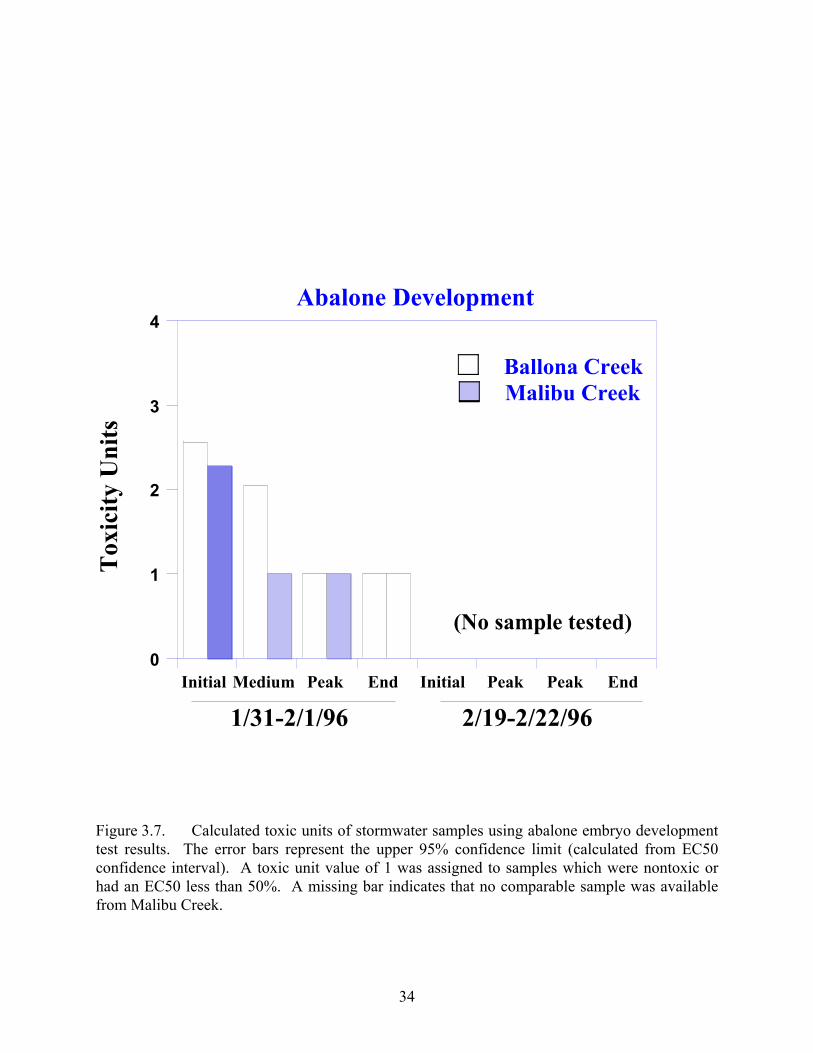
3.4 Relative Toxicity Between sites A comparison of relative toxicity between Ballona Creek and Malibu Creek cannot be made for samples from 1/16/96 and 1/21/96 since very little stormwater was present in Malibu Creek. Results from the two collection events in February can be compared by calculating the toxic units (100/EC50) for each sample. The most complete comparison can be made using fertilization test data. The first sample collected from Malibu Creek during each storm was not used for comparison since little stormwater was present. Comparison of the toxic units calculated for the other samples shows that Ballona Creek stormwater was always more toxic than samples from Malibu Creek (Figure 3.6). Comparison of the abalone embryo test results for 1/31/96 - 2/1/96 samples shows a similar pattern: Ballona Creek samples were usually toxic, while no toxicity was detected in comparable Malibu Creek samples (Figure 3.7). Between species Lower EC50 values were usually calculated from the sea urchin fertilization data (Table 3.10), indicating that this test was more sensitive to stormwater quality than was the abalone embryo development test. This result was surprising, considering that the abalone embryo test is of much longer duration. 3.5 Toxicity Identification Evaluation One sample from Ballona Creek was selected from each of the four storm events for phase I TIE analysis. A range of flow conditions (initial, medium, and peak) was represented by these samples. In addition, one sample collected on 2/1 from Malibu Creek (peak flow) was also prepared for TIE evaluation. No artifacts or interferences were introduced by the various TIE manipulations; controls for the salinity adjustment, filtration, solid phase extraction, and thiosulfate treatments all had fertilization percentages that were similar to the seawater control. Although two or three replicates were tested for each treatment group (see data appendix), only those samples needed to identify the pattern of response were examined. At a minimum, all replicates of the blanks and samples at the 50% test concentration were counted. Each of the Ballona Creek samples showed a remarkably similar pattern of response to the TIE treatments (Figure 3.8). Treatment with EDTA (3 mg/L final concentration) completely removed the toxicity in each case. Filtration and sodium thiosulfate addition were not effective on any of the samples. Solid phase extraction (SPE) partially removed toxicity on only the last sample from Ballona Creek (2/19/96). The baseline (pre-filter) toxicity in three of four samples was similar to that measured in the first test, conducted 6 - 10 days earlier. This result indicated that the toxicants were relatively stable in solution.

32

2468

1012141618

Initial Med Peak End Initial Peak Peak End

Tox

icity

Uni

ts

1/31-2/1/96 2/19-2/22/96

Ballona CreekMalibu Creek

Sea Urchin Fertilization 0 Figure 3.6. Calculated toxic units of stormwater samples using sea urchin fertilization test results.

The error bars represent the upper 95% confidence limit (calculated from EC50 confidence interval). A toxic unit value of 1 was assigned to samples which were nontoxic or had an EC50 less than 50%. A missing bar indicates that no comparable sample was available from Malibu Creek.

33

1

2

3

4

Initial Medium Peak End Initial Peak Peak End

Ballona CreekMalibu Creek

Tox

icity

Uni

ts

1/31-2/1/96 2/19-2/22/96

Abalone Development

(No sample tested)0

Figure 3.7. Calculated toxic units of stormwater samples using abalone embryo development test results. The error bars represent the upper 95% confidence limit (calculated from EC50 confidence interval). A toxic unit value of 1 was assigned to samples which were nontoxic or had an EC50 less than 50%. A missing bar indicates that no comparable sample was available from Malibu Creek.

34

A somewhat different response pattern was obtained for the Malibu Creek sample following the TIE treatment sequence. EDTA completely removed the toxicity (similar to Ballona Creek samples), but partial toxicity reductions were also produced by filtration and sodium thiosulfate addition (Figure 3.9). The consistent effectiveness of EDTA and limited removal of toxicity by SPE suggests that cationic metals are likely sources of the toxicity. EDTA complexes with many divalent trace metals and renders them nontoxic (Figure 3.10). Thiosulfate also has a similar effect on some metals. The variations in response pattern suggest that some of the toxic components present in Malibu Creek stormwater are different from those present in Ballona Creek. The TIE response pattern suggests that zinc, lead, nickel, and manganese are the metals most likely to be associated with Ballona Creek runoff toxicity. The partial effectiveness of thiosulfate in reducing toxicity in the Malibu Creek sample suggests that copper, cadmium, or mercury may be contributing to the toxicity at this site. Chemical analysis results of the stormwater samples are needed to evaluate whether the TIE results are plausible.

35

20

30

40

50

60

70

80

90

100

10 20 30 40 50 60

RawPost C18EDTAThiosulfate

% o

f con

trol

dev

elop

men

t

1/21/96

0

20

40

60

80

100

10 20 30 40 50 60

RawPost C18EDTAThiosulfate

% o

f con

trol

dev

elop

men

t

1/31/96

0

20

40

60

80

100

10 20 30 40 50 60

RawPost C18EDTAThiosulfate%

of c

ontr

ol d

evel

opm

ent

Sample Concentration (%)

2/19/96

Figure 3.8. Summary of TIE results for Ballona Creek stormwater samples. Raw refers to

stormwater without treatment. Error bars are standard deviations.

36

0

20

40

60

80

100

10 20 30 40 50 60

Raw Post C18

EDTA Thiosulfate %

of c

ontr

ol d

evel

opm

ent

Sample Concentration (%)

1/31/96

Figure 3.9. Summary of TIE results for a sample of Malibu Creek stormwater. Raw refers to

stormwater without treatment. Error bars are standard deviations.

37

Figure 3.10. Interaction of cationic metals with TIE procedures. Results are those obtained

with Ceriodaphnia dubia in freshwater (Norberg-King, 1996). Toxicity removed by EDTA No effect with EDTA

Cd Ag Toxicity removed by thiosulfate Cu Se (selenate) Hg

Zn Fe Mn Cr (III) No effect with Thiosulfate Pb Cr (IV) Ni As (arsenite or aresenate) Se (selenite)

38

4.0 CONCLUSIONS This study sampled stormwater from two major storm drains that flow to Santa Monica Bay. Water quality, dissolved metals and target GC/MS (base/neutral compounds) were analyzed. Toxicity analyses of several storm events were also performed. The following conclusions are presented: 1. All samples of Ballona Creek were toxic. 2. Only one sample from Malibu Creek were toxic. 3. Toxicity Identification of positive samples implicated metals as the most likely cause of the

toxicity. Post-C18 toxicity was generally not improved, indicating that organic compounds were not responsible. Thiosulfate addition did not decrease toxicity for Ballona Creek samples; thiosulfate addition decreased toxicity in the one Malibu sample that was toxic.

4. Insufficient data were collected to perform correlations of water quality data with toxicity; however, future studies should be designed to identify the responsible metals.

39

40

5.0 REFERENCES ASCE (1960). Design and Construction of Sanitary and Storm Sewers, Manual of Practice. Chapman, G.A., Denton, D.L., and J.M. Lazorchak (1995). Short-term Methods for Estimating

the Chronic Toxicity Effluents and Receiving Waters to West Coast Marine and Estuarine Organisms. EPA/600/R-95-136, Office of Research and Development, US Environmental Protection Agency, Cincinnati, OH

Lau, S-L. and M.K. Stenstrom (1997), “Solid Phase Extraction for Oil and Grease Analysis,”

Water Environment Research, Vol. 69, No. 3, pp. 368-374. Makepeace, D.K., Smith, D.W., and S.J. Stanley (1995). “Urban Stormwater Quality: Summary

of Contaminant Data,” Critical Review of Environmental Science and Technology, Vol. 25, No. 2, pp. 93-139.

Norberg-King, T.J., D.I. Mount, J.R. Amato, D.A. Jensen, and J.A. Thompson (1992). Toxicity

Identification Evaluation: Characterization of Chronically Toxic Effluents, Phase I. EPA/600/6-91/005F, Environmental Research Laboratory, Office of Research and Development, U.S. Environmental Protection Agency, Duluth, MN 55904.

Stenstrom, M.K. and E. Strecker (1993), “Assessment of Storm Drain Sources of Contaminants

to Santa Monica Bay, Vol. I, Annual Pollutants Loadings to Santa Monica Bay from Stormwater Runoff,” UCLA-ENG-93-62, Vol. I, pp. 1-248.

Wong, K., E.W. Strecker and M.K. Stenstrom (1997), “A Geographic Information System To

Estimate Stormwater Pollutant Mass Loadings,” Journal of the Environmental Engineering Division, ASCE, Vol. 123, pp. 737-745.