Assessment of scale of hazards due to pool fire for a...

MAUSAM, 60, 2 (April 2009), 197-210

504.4 : 551.556.42

(197)

Assessment of scale of hazards due to pool fire for a

fossil fired power plant in India

ARUN KUMAR, S. K. DASH and S. K. DHAKA*

Centre for Atmospheric Sciences, IIT Delhi, India

*Department of Physics, University of Delhi, India

(Received 28 September 2007, Modified 2 March 2009)

e mail : [email protected]; [email protected]; [email protected]

lkjlkjlkjlkj & bl 'kks/k i= esa Hkkjr esa xqtjkr jkT; ds rV ij fLFkr QkWfly Qk;MZ ikoj IykaV ds dkj.k gksus okys tksf[ke dk vkdyu fd;k x;k gS! QkWfly Qk;MZ ikoj IykaV dh Vadh ls fiPNd ¼Iywe½ ds izs{k.k iFk vkSj QSyko dk vuqeku yxk;k x;k gSA ;g vuqeku 'khrdky vkSj xzh"edky esa fnu vkSj jkr ds le; dh de vkSj vf/kd iou xfr ds izs{k.k ds nkSjku dkVZj] feYl] fczXl vkSj tksukVksa uked orZeku esa iz;qDr fun’kkZsa dk mi;ksx djds yxk;k x;k gSA ifj.kkeksa ls irk pyk gS fd xzh"e _rq ds nkSjku pyus okyh nf{k.k if’peh vkSj nf{k.kh gokvksa ds dkj.k ikoj IykaV ds mRrj iwoZ esaa foLr`r {ks= esa QSyh fjgk;’kh vkcknh dks [kRkjk gks ldrk gSA lqcg ds le; ;k nsj jkr dks tc iou dh xfr de gksrh gS rc fi{Nd ¼Iywe½ dh m¡pkbZ vkSj pkSM+kbZ vf/kd ikbZ xbZ gSA nksigj ds vklikl tSls gh iou dh xfr c<+rh gS fi{Nd ¼Iywe½ dh m¡pkbZ vkSj pkSM+kbZ esa deh vkrh gSA ok;q dh xfr de gksus ij ySaFk Ldsy de gks tkrk gS vkSj ok;q dh xfr vf/kd gksus ij ySaFk Ldsy vf/kd gks tkrk gSA [krjs dh fLFkfr;ksa ds nkSjku 70 eh- dh f=T; nwjh ds vkxs rkih; fofdj.k dh ?kkrd ek=k vkSlr lhek ds vanj gSA

ABSTRACT. Hazards for a fossil fired power plant located at coastal Gujarat in India have been assessed. The

trajectory and spread of the plume from tanks of fossil fired power plant were predicted using existing models named Carter, Mills, Briggs and Zonato during winter and summer seasons with low and high wind speeds observed in day and night hours. Results show that wide areas of habitation and human settlement to the northeast of the site may be potentially under hazards due to southwesterly and southerly winds during summer. Plume heights and widths are found high in the morning hours or late night when wind speeds are low. As wind speed increases around noon, low plume heights and widths are obtained. Length scales become low at low wind speeds and vice-versa. Lethal doses of thermal radiation beyond radial distance of 70 m are within the tolerable limit under hazardous condition.

Key words ‒ Pool fire, Lateral and vertical spread, Length scale, Plume height, Plume width.

1. Introduction

Pool fires occur when flammable liquids ignite and

burn due to accidental rupture of fuel storage vessels. This type of fire is particularly risky since a wide range of potentially hazardous combustion products may be evolved (Atkinson and Jagger, 1992, Fisher et al., 2000). The resultant smoke plumes disperse in the direction of downwind across the residential areas and threaten the lives and properties of local population (Hall et al., 1995, Carruthers et al., 1999). Toxic smoke and other combustion products may lead to population evacuation and even small doses of chemicals can cause ill effects. The horizontal motion of plume is governed by prevailing wind and vertical motion is determined by buoyancy. It is a function of initial density distribution within the plume

cross-section and atmospheric stratification (Ghoniem et al., 1993). The density of plume is determined by temperature and smoke concentration of the pool-fire. As the plume rises, both varies due to entrainment and mixing with surrounding air; its diameter grows and internal velocities decay until these are comparable with scales of length and velocity of ambient turbulence. Plume breaks up rapidly within the inertial sub range. The turbulent energy at a given length-scale (distance at which plume terminates) is determined by turbulent dissipation rate. If the scale of thermals is much larger than that of plume, the plume will rise relative to surrounding updrafts or downdraft. Plume may loop strongly and rise in the mean direction. In the present study, four models namely Briggs, Mills, Carter and Zonato are used to predict lateral and vertical spread, plume width, plume height, hydraulic

198 MAUSAM, 60, 2 (April 2009)

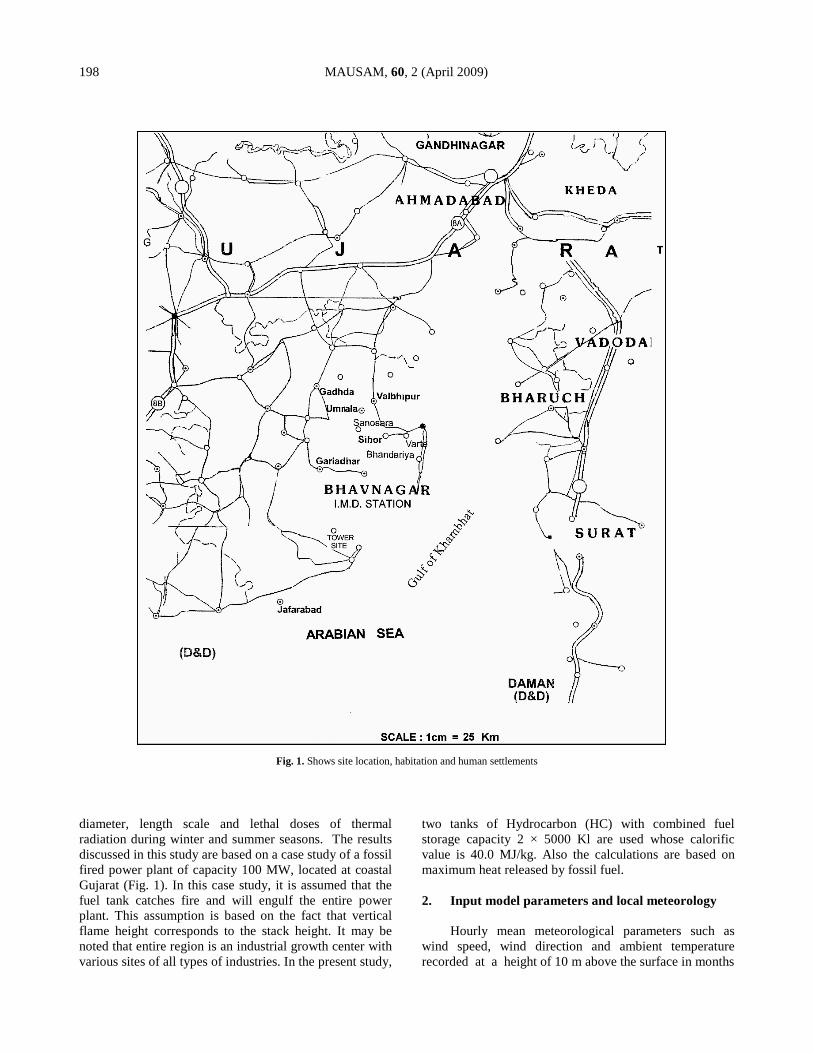
Fig. 1. Shows site location, habitation and human settlements diameter, length scale and lethal doses of thermal radiation during winter and summer seasons. The results discussed in this study are based on a case study of a fossil fired power plant of capacity 100 MW, located at coastal Gujarat (Fig. 1). In this case study, it is assumed that the fuel tank catches fire and will engulf the entire power plant. This assumption is based on the fact that vertical flame height corresponds to the stack height. It may be noted that entire region is an industrial growth center with various sites of all types of industries. In the present study,

two tanks of Hydrocarbon (HC) with combined fuel storage capacity 2 × 5000 Kl are used whose calorific value is 40.0 MJ/kg. Also the calculations are based on maximum heat released by fossil fuel. 2. Input model parameters and local meteorology

Hourly mean meteorological parameters such as wind speed, wind direction and ambient temperature recorded at a height of 10 m above the surface in months

KUMAR et al. : HAZARDS DUE TO FOSSIL FIRED POWER PLANT 199

TABLE 1

Input parameters used in models

Parameters Values

Tank height 55 m

Tank diameter 16 m

Tank capacity 8.5 × 106 Kg

Caloric value 80.9 × 109 Kcal

Heat rate 1850 Kcal / KWh

Caloric value of fuel 80.9 × 109 Kcal

Heat release rate of fuel 43.7 × 103 MWh

Ambient temperature 298 K

Specific heat capacity of pool fire fuel 1.012 KJKg -1 K-1

Entrainment parameters 0.6

Density of air 1.25 Kg m-3

of January and May 2005 are used in this study. In India January and May months may be considered to represent winter and summer seasons respectively. Effective heat release rate (QE), total heat release rate (QH) from source, density of air (ρ), specific heat (Cp), ambient temperature (Ta) and acceleration due to gravity (g) are used to calculate buoyancy flux FB and plume height by Briggs and Mills models. Plume centerline height (Hi) is considered for all models. Hi is replaced by HB, HM, Hca and Hzo for Briggs, Mills, Carter and Zonato predicted plume central heights respectively.

It is assumed that these values do not vary much over wide range of conditions, so that buoyancy flux FB is proportional to QE. Input parameters and their numerical values are given in Table 1.

Meteorological conditions of a place have an

important role in dispersion of plume. Hourly wind speed, wind direction and ambient temperature are measured at 10 m height above the surface. Further vertical variation of wind speed computed at stack height (55 m) by power law (CPCB India 1997) is used in models. Northeasterly is strong in winter and southwesterly is strong in summer. Areas to the north and northeast of the site (Fig. 1) are densely populated and hence southwesterly and southerly strong winds in summer may be potentially hazardous. Ambient temperatures are moderate in the region as the site is located at the Arabian Sea coast. The ranges of diurnal variation of temperatures are 15 to 20° C in winter and 30 to 35° C in summer. It is observed that humidity is low in winter and high in summer. During summer before the commencement of southwest monsoon the humidity attains the value generally up to 61%. Low cloudiness (< 3 ocktas of sky) is noted.

2.1. Calculation of stability class

The solar isolation based classification as recommended by Central Pollution Control Board India, (1997) has been used to determine hourly atmospheric stability for January and May months representing winter and summer seasons. In case of unavailability of incoming solar radiation data, the following parameters are calculated to estimate solar insolation and hourly stability. Solar declination (Ds) determines Sun’s position with respect to the celestial equator, whose value changes from 23.5° N to 23.5° S in a year due to inclination of the axis of earth’s rotation to the ecliptic plane. Ds is calculated using the function,

( )

+=N

n π2842Sin3.45Ds (1)

Here N is the total number of days in a year (365 or

366) and n is the number of day starting from January 1 as the first day (i.e., n = 31 for 31st January). Apparent local time ta (in hours) represents Sun’s position, as it actually appears by calendar time tc, local time and EQT correction term and is given by,

60

EQT

15

MM stdlocca +−+= tt (2)

where, EQT stands for Equation of Time, Mloc

(M loc = 72.11° E) and Mstd (Mstd = 82.5° E in India) are local and standard reference meridians respectively, tc is calendar time. At any location, the time at which Sun crosses the meridian is called local noon which is different from the noon based on standard time. It may be noted that the difference between mean and apparent solar time is called EQT calculated in minutes as given below:

( ) ( )

−+

−−=N

n

N

n π802sin9.5

π32sin7.7EQT

(3) The hour angle t is defined as the arc of the circle

along the celestial equator measured from the upper meridian of the observer to that of the sun. t is expressed in terms of angle measured east and westwards and is equal to 15 (12 - ta) degrees. Solar elevation angle h is calculated by site latitude, solar declination and hour angle of the Sun at the specified hour by the function, sin (h) = sin (L).sin (Ds) + cos (L).cos (Ds).cos (t), where L is latitude of the site (21.75° N), t is hour angle of the Sun and Ds is solar declination. Solar isolation based on cloud cover and solar angle (h) is determined. Stability

200 MAUSAM, 60, 2 (April 2009)

TABLE 2

Atmospheric stability results

Day hours 07 08 09 10 11 12 13 14 15 16 17 18

Winter

Wind speed (m/s) 0.67 0.67 1.00 1.56 2.23 3.01 3.56 3.96 3.94 3.87 3.49 3.2

Stability B B B B B A B B C C C C

Summer

Wind speed (m/s) 3.61 3.55 3.25 3.07 3.43 4.66 4.84 5.26 5.40 5.17 4.83 4.7

Stability C C C B B B B C D D C C

Night hours 19 20 21 22 23 24 01 02 03 04 05 06

Winter

Wind speed (m/s) 2.8 2.5 2.3 2.2 2.1 2.0 1.9 2.0 1.8 1.5 1.3 1.0

Stability F F F F F F F F F F F F

Summer

Wind speed (m/s) 4.7 4.2 3.4 3.3 3.3 3.1 3.8 4.1 4.0 4.1 3.0 2.8

Stability E E E E E E E E E E E F

classes in day hours are determined by surface wind speed (m/s) and insolation category and at night by cloud cover and wind speed. Night refers to the period half hour after sunset and half hour before sunrise CPCB, India (1997) and day hours considered in study is 0700 to 1800 hours (IST). Atmospheric stability calculated with hourly mean wind speed is given in Table 2. 3. Model details

3.1. Carter model

In Carter (1989) model the fire source is considered

as a source of buoyant smoke for subsequent dispersion and is represented by a specific mass burning rate and vertical flame height influenced by prevailing wind direction. It is assumed that the environment radiates 15% of the total heat released, 10% of the total volume is unburned and the remainder is stochiometrically converted to gaseous products (Fisher et al., 2000). In the present case, stack height H, tank effective diameter D and hourly wind speed recorded at the site at 10 m height are used as input data in model. The model is developed on the assumption that the dilution of a rising plume is essentially a three dimensional process. At any instant the plume would therefore be lumpy and consist of a series of maxima concentrations along the axis and zero

concentrations in between. The momentum terms are excluded for the large buoyant releases from the tanks. The plume rise (Hca) is represented as below,

( )[ ]10m

1/4

eff2

effEca

27QAH

u

DXX +×= (4)

Where, A is a constant term whose values depend

upon heat release rate, QE whose values are 2.25 and 0.395, expressed in MW and KW respectively. Xeff is modified distance and D is effective diameter of pool-fire. u10m is wind speed (m/s) observed at 10 m height above the surface. QE is represented in terms of total rate of release of energy QH from the pool fire. QE = (1- ε)QH. QH is 5.15 Kwh / kg (at heat rate of 1850 Kcal/Kwh). Radiant emission fraction ε = 0.25. Modified distance Xeff is expressed in terms of actual distance X and length scale Xt as below,

( )22eff

t

t

XX

XXX

+= (5)

It is assumed that plume rise is terminated at a

distance Xt in down wind direction and achieves a


corresponding plume height Hca. Xt is represented by the function,

( )22ns

nst

XX

XXX

+= (6)

The above function has been chosen for

smaller values of terms Xs and Xn. Xs is given by, Xs = 120 (U10 / √Γ). Here Γ is the potential temperature gradient = 0.08 K at (100m)–1 adopted by Moore (1980) and u10m is of order of 5 m/s. Xn = 19.2 (100 + H). Here, H is the vertical flame height, which corresponds to the stack height as suggested by Moore (1974 and 1980). The model is applicable to wide range of atmospheric conditions and accounts for the effect of wind generated turbulence and plume rise termination.

3.2. Mills and Briggs models

Mills (1987) shows behaviour of plume by considering effective diameter of pool fire. It is assumed that 30% of the heat released by the fire is actually radiated to the environment and does not contribute to the plume buoyancy. It is assumed that plume gases have similar specific heat and molecular mass as of hot air Fisher et al., (2000). The plume buoyancy flux is computed by using the relation,

aTp

EB πρC

gQF = (7)

where, ρ = 1.25 kg m-3 is the density of air,

Cp = 1.012 KJ kg-1 K-1 is specific heat of the evolved gases (that for air) and Ta = 298 K is ambient air temperature for Indian conditions. It is assumed that the parameters do not vary much over the range of conditions. The Mills plume rise equation is based on Briggs equation for the rise of bent over two-dimensional buoyant jet. Term D is used by Mills in modification of Briggs model. Thus, Mills plume rise for buoyant plume is given by the function,

2β2βHH

1/333BM

DD −

+= (8)

where,

10m

2/31/3B

1/3

2BF

2β

3H

u

X

= (9)

Here, HB is Briggs plume rise in which the constant

term

1/3

22β

3

= 1.609. Briggs equation is used to

calculate plume rise from a point source in two-dimensional buoyant jet. Mills modified Briggs equation (Eqn. 9) and introduced effective diameter of the pool fire, which reduces plume rise (X < 100 m). β is entrainment parameter for bent over buoyant plume. It is assumed that plume appears as a continuous cone, which is bent over, rising and expanding, so that entrainment of air into the cone is two dimensional at the surface of the plume.

3.3. Zonato model

Zonato et al. (1993) compared his experimental values with that of Mills and Carter considered the dimensional dependence of the plume rise trajectory on the empirical values of variables on the basis of least -square regression to fit plume-rise trajectory Hunt and Weber (1979). The plume rise of Zonato is represented by,

( )[ ] cba ux −−= 10HZO Qε1dH (10)

Zonato used the parameter values, similar to those of

Carter and Mills. Hence the plume rise trajectory are represented by

( )[ ] -0.510

0.630.26HZO Qε10.38H uX−= (11)

( )[ ] -0.510

0.630.26HZO Qε14.2H uX−= (for X/D > 45)

(12) Zonato et al. (1993) observed deviation of 10% from

those observed by Carter and Mills results. The lateral and vertical spreads σy and σz are calculated by Bennett et al. (1992) from the relation, σy = 0.32 Hi and σz = 0.27 Hi. Here, Hi is plume rise predicted by models, which is a function of downwind distance X. Bennett et al. (1992) and Bennett (1995) used lateral and vertical plume widths at top hat distribution of material with instantaneous concentration profile, wy = 0.55 Hi and wz = 0.47 Hi which are in good agreement with theoretical values used in derivation of plume rise.

3.4. Calculation of hydraulic diameter Hydraulic diameter (Dh) is calculated in spill area for

the large source CPCB, India (2001). It is assumed that emissivity of the flame (εf) = 1 for the large source of attenuation coefficient x. The burning rate from the pool is sum of evaporation rates due to heat transfer from ground

202 MAUSAM, 60, 2 (April 2009)

and inward radiation and heat transfer from the flame. Liquid regression rate Va (mh-1) is calculated by function,

( )xDha eV −−

= 1

Q

Q00456.0

v

E (13)

Here, Qv is heat of vaporization. Since, Heat of

vaporization is insignificant as compared to that heat of combustion. Va can be written as, Va = 0.00456 QE for QE >> Qv and 1-e-xDh =1 (for large source). Heat transfer from flame, m (kg m-2s-1) = Va (ρL/3600). It is assumed that heat transfer from flame (m) >> heat transfer from ground (m′). Ratio of plume height (Hi) to hydraulic diameter (Dh) is given by,

( ) ( ) 0.044*0.252

0.5

a

i gρ

6.2H −

= uD

m

D hh

(14)

Where, ρa = 1.2 (kg m-3) is density of air,

g = 9.8 m s-2 is acceleration due to gravity and u * = (g m Dh / ρa)

1/3 is velocity of fuel leaving at interface.

3.5. Estimate of Lethal doses of thermal radiation

Probit equation CPCB, India (2001) is applied to calculate thermal radiation, which is function of intensity of radiation received and time of exposure. It is given by,

Y = K1+ K2 lnV (15)

Where, Y is probit, K1 (K1=14.9) and K2 (K2 = 2.56) are constants and V is causative variable defined by, V = t l 4/3 (10 - 4). l is incident heat flux (KW/m2) and t is time of exposure in second. Probit equation estimates lethality is expressed as,

( )[ ]43/4 10lln56.29.14Y −+−= t (16)

for the surface area of radii 5 m to 100 m.

3.6. Comparison of models Carter’s model comprises of three-dimensional

processes where pool fires break into discrete lumps or puffs. These puffs merge into one another and drift into downwind direction. Plume appears to evolve from the imaginary source at a point upwind and beneath the fire and have the horizontal cross sectional area equivalent to the actual source as it passes though the fire. Carter considered a modified version of Moore formula (Moore, 1980; Jones, 1983) to estimate plume-rise. The potential temperature gradient, Γ = 0.08 (100 m)-1 is used to account temperature at 100 m height. Plume rise

terminated (Eqn. 5), when it traveled length-scale Xt (X < Xs or Xn and Xeff = X). The model is applicable for all atmospheric conditions occurring in day and night hours.

In Mills model, effective diameter of pool fire is introduced and used to calculate plume rise, which is bent over two-dimensional buoyant jet in all atmospheric conditions as in Briggs model and used effective diameter of the pool fire. The entrainment parameter (β) is used in the model to account for bent over of buoyant plume. Plume buoyancy flux is considered in the model to account buoyancy of the pool fire, which is similar to that of hot air. In Briggs and Mills model, plume dilution or decrease of plume rise by ground attenuation has not been considered; also reflection coefficient in first and subsequent reflections of plume from the ground has not been included in the study of plume behaviour.

Zonato model is based on observations. He made use

of observational values in empirical relations based on least-square regression to fit plume rise trajectory. a, b, c and d are empirical coefficients used in the model. Results show similar plume behaviour with diurnal variation of wind. It is observed that plume rise and width are function of down wind. It is comparable to the results obtained by Carter, Mills and Briggs. Radiant emission factor (ε) is applied to account for unused percentage of fuel, which is either unburned or radiated into the environment. It is similar to that assumed by Mills and Briggs. Zonato found that maximum deviation of predicted values is 10 % compared to other models. 4. Results

The study employs a workable and easily adaptable

procedure to assess hazards for a fossil fired power plant located at a coastal area in Gujarat. Briggs, Mills, Carter and Zonato models are used to predict lateral and vertical spreads, plume width, plume height, hydraulic diameter and length scale with diurnal variation of wind speed during winter and summer seasons. Similar parameters are predicted at mean wind speeds 2.28 m/s in winter and 4.0 m/s in summer at different locations. Here, locations 1, 2, 3 up to 24 correspond to 5, 10, 15, 20, 25, 30, 35, 40, 45, 50, 60, 70, 80, 90,100, 110, 120, 130, 140, 150, 160, 170, 180, 200 m down wind distances respectively from the source. Hazardous effect of lethal doses of thermal radiation at the ground exposed for 20 sec at different radial distances are also predicted. Input parameters as discussed in Table 1 are similar for all models. Predicted plume height, lateral and vertical spreads and plume width and hydraulic diameter are influenced by meteorological conditions and are dispersed into the direction of prevailing wind.


Fig. 2. Wind roses in (a) winter and (b) summer

Figs. 3(a&b). Diurnal variation of observed wind speed (m/s) and predicted lateral, vertical plume spreads (m) by Carter, Briggs, Mills and Zonato in (a) winter (b) summer

0

8

16

24

32

1 2 3 4 5 6 7 8 9 10 11 12 13 14 15 16 17 18 19 20 21 22 23 24

Hours

Spr

ead

2

4

6

8

10

12

14

1 2 3 4 5 6 7 8 9 10 11 12 13 14 15 16 17 18 19 20 21 22 23 24

Hours

Spr

ead

Wind speed Lateral spread andVertical spread by Briggs Lateral spread andVertical spread by Mills Lateral spread andVertical spread by Carter Lateral spread andVertical spread by Zonato

Winter

Summer

(a)

(b)

204 MAUSAM, 60, 2 (April 2009)

TABLE 3

Predicted plume heights, widths and hydraulic diameters at minimum and maximum wind speeds during (a) winter (b) summer

Plume spread (m) Plume width at top hat (m) Wind Speed (m/s)

Plume height (m)

Lateral Vertical Lateral Vertical

Hydraulic Diameter (m)

Model

Day Night Day Night Day Night Day Night Day Night Day Night Day Night

(a) Winter

0.6 1.0 94.4 72.4 30.2 23.1 25.5 19.5 51.6 39.8 44.4 34.0 1.7 1.4 Carter

3.9 2.8 23.5 32.2 7.5 10.3 6.3 8.7 12.9 17.7 11.0 15.1 0.7 0.8

0.6 1.0 62.4 54.2 19.9 17.3 16.8 14.6 34.3 29.8 29.3 25.5 1.3 1.2 Briggs

3.9 2.8 34.5 38.6 11.0 12.3 9.3 10.4 18.9 21.2 16.2 18.1 0.9 0.9

0.6 1.0 49.3 41.2 15.7 13.1 13.3 11.1 27.1 22.6 23.1 19.3 1.1 1.0 Mills

3.9 2.8 21.8 25.8 6.9 8.2 5.9 6.9 12.0 14.2 10.2 12.1 0.6 0.7

0.6 1.0 18.7 19.8 6.0 6.3 5.0 5.3 10.3 10.9 8.8 9.3 0.6 0.6 Zonato

3.9 2.8 23.6 22.6 7.5 7.2 6.3 6.1 13.0 12.4 11.1 10.6 0.7 0.6

(b) Summer

3.0 2.8 29.8 32.0 9.5 10.2 8.0 8.6 9.5 10.2 8.0 8.6 0.8 0.8 Carter

5.4 4.7 17.5 20.0 5.6 6.4 4.7 5.4 5.6 6.4 4.7 5.4 0.5 0.6

3.0 2.8 37.5 38.5 12.0 12.3 10.1 10.4 12.0 12.3 10.1 10.4 0.9 0.9 Briggs

5.4 4.7 31.1 32.6 9.9 10.4 8.4 8.8 9.9 10.4 8.4 8.8 0.8 0.8

3.0 2.8 24.8 25.7 7.9 8.2 6.7 6.9 7.9 8.2 6.7 6.9 0.7 0.7 Mills

5.4 4.7 18.6 20.0 5.9 6.4 5.0 5.4 5.9 6.4 5.0 5.4 0.6 0.6

3.0 2.8 22.8 22.6 7.3 7.2 6.1 6.1 7.3 7.2 6.1 6.1 0.6 0.6 Zonato

5.4 4.7 24.6 24.2 7.8 7.7 6.6 6.5 7.8 7.7 6.6 6.5 0.7 0.7

Strong northeasterly to northwesterly is the favourable wind direction in winter and southwesterly to southerly is prevalent in summer (Fig. 2). Figs. 3 (a&b) respectively show that wind speeds attain maximum value of 3.01-3.96 m/s in winter and 5.17-5.40 m/s in summer.

Clarke, 1979 atmospheric stability is applied on the basis of hourly mean wind speed, solar isolation during day hours and cloud cover at night hours. Stability classes A, B, C and D indicate the dominance of unstable and neutral atmospheric conditions respectively during day hours and E and F represent stable atmospheric conditions dominate during night hours (Table 2).

The results predicted by the models of Briggs, Mills,

Carter and Zonato show that lateral and vertical spreads are high at low wind speeds and vice versa and former is followed by latter (Fig. 3). The predicted values by Carter model are high at low wind speed, which are followed by Briggs and Mills values. Zonato predicts low values at

low wind speed of 0.6 m/s under stability class B. Under similar atmospheric stability and at high wind speed (3.9 m/s), the predicted values of lateral and vertical spreads by Briggs model are high which are followed by predicted values of Carter and Mills models result.

Zonato model predicts low value. Similar features

are found during night, the predicted values of lateral and vertical spreads by Carter model are high which are followed by Briggs, Mills and Zonato at low wind speed of 1 m/s and at high wind speed 2.8 m/s under atmospheric stability F, the predicted values of lateral and vertical spreads by Briggs are high which is followed by values of Carter and Mills models. Zonato model predicts low value [Table 3 (a)]. It is noted that at low wind speed (< 2.0 m/s), Carter model predicted high value, which is followed by Briggs, Mills and Zonato and as wind speed increases and attains value of 3.9 m/s, Briggs model predicts high value that is followed by Carter, Mills and Zonato models (Table 3) in day hours.


Figs. 4(a&b). Diurnal variation of observed wind speed (m/s) and predicted plume-widths (m) by Carter, Briggs, Mills and Zonato in (a) winter (b) summer

Lateral and vertical Plume widths [Fig. 4 (a)] at top

hat distribution predicted by Carter model are high, which are followed by Briggs, Mills and Zonato models at low wind speed (0.6 m/s) under stability class B. Under similar atmospheric stability and at high wind speed (3.9 m/s), the predicted values of lateral and vertical plume widths by Briggs and Mills models are high and predicted values of Carter model lie in between them. Wind speed is comparatively low during night, the predicted values of lateral and vertical plume widths by Carter model are high at wind speed 1 m/s which are followed by predicted values of Briggs, Mills and Zonato models and at high wind speed (2.8 m/s) under atmospheric stability F, Briggs model predicts high values (Table 3) in winter which are followed by predicted values of Carter, Mills and Zonato models.

During summer, wind speeds are high and lateral and

vertical plume spreads are low. The predicted values of

lateral and vertical spreads by Briggs are high, which are followed by Carter, Mills and Zonato models predict low values at wind speed of 3.0 m/s under stability class B (Table 3). As wind speed increases to 5.4 m/s under stability class D, high values of lateral and vertical spreads are predicted by Briggs model, which are followed by predicted values of Mills and Carter models result during day hour. Zonato model predicts low value. During night, the predicted values of lateral and vertical spreads by Briggs are high, which are followed by Carter, Mills and Zonato at wind speed of 2.8 m/s under atmospheric stability F.

It is found that lateral and vertical plume widths,

predicted by Carter model is high at low wind speed and as wind speed increases (> 2.0 m/s), Briggs model predicts higher values. It is noted that the values of plume width at top height is large (as w/σ = 1.7) compare to plume spread under same atmospheric conditions. At

0

11

22

33

44

55

1 2 3 4 5 6 7 8 9 10 11 12 13 14 15 16 17 18 19 20 21 22 23 24Hour

Plu

me

wid

th

0

5

10

15

20

25

1 2 3 4 5 6 7 8 9 10 11 12 13 14 15 16 17 18 19 20 21 22 23 24

Hour

Plu

me

wid

th

Wind speed Lateral plume width andVertical plume width by Briggs Lateral plume width andVertical plume width by Mills Lateral plume width andVertical plume width by Zonato Lateral plume width andVertical plume width by Carter

Winter

Summer

(a)

(b)

206 MAUSAM, 60, 2 (April 2009)

Figs. 5(a&b). Predicted plume heights by Carter, Briggs, Mills and Zonato at different locations in (a) winter at mean wind speed 2.28 m/s and (b) summer at mean wind speed 4.4 m/s

mean wind speed (2.2 m/s) and at different radial distances (≤ 200 m) during winter, lateral and vertical spreads predicted by models of Briggs and Mills are constant and values predicted by Carter and Zonato models are low close to the source (at X = 5m) and increases with distance (Eqn. 5). Maximum value of lateral and vertical spreads predicted by Carter and Zonato models are 17.3 and 14.6 m and 33.8 and 28.5 m respectively at 200 m from the source.

The results predicted by the models show (Fig. 4)

that plume height predicted by Carter model results are high which is followed by Briggs, Mills and Zonato models result at low wind speed (0.6 m/s) and at high wind speed (3.9 m/s) plume height predicted by Briggs model is high which is followed by Carter, Mills and Zonato models respectively during winter under atmospheric stability B in day hours (Table 3).

During night, predicted values by the models results

show that plume heights are high at low wind speed of 1.0 m/s and low with values at high wind speed of 2.8 m/s

under stability class F during winter. In summer; plume heights predicted by Briggs model are high at low wind speed (3.07 m/s) under stability class B and low at high wind speed (5.4 m/s) under neutral atmospheric stability class D in day hours. During summer at mean wind speed 4.0 m/s, maximum plume height predicted by Briggs model is 40.8 m at 200 m distance from the source. Predicted plume height by Briggs is higher than that of Mills as effective plume diameter is used by Mills model results, which reduces the plume height. Zonato model shows that plume height is high at low wind speed and vice versa. Consequently, High plume height is predicted in winter and low in summer as plume height depends on wind speed shown at denominator in Eqn. 10. It agrees with Fisher et al. (2000) study of plume behaviour at mean wind speed. Hydraulic diameters are predicted in each stability class during winter and summer seasons using plume heights predicted by models of Carter, Briggs, Mills and Zonato. It is found that diameters are low at high wind speeds and vice-versa (Fig. 6). High hydraulic diameter (1.7m) is predicted by Carter model at low wind speed 0.6 m/s during winter under atmospheric stability B. Further at high wind speed of 3.9 m/s, Briggs

020406080

100

1 2 3 4 5 6 7 8 9 10 11 12 13 14 15 16 17 18 19 20 21 22 23 24

Hours

Plu

me

Hei

ght

0

10

20

30

40

50

1 2 3 4 5 6 7 8 9 10 11 12 13 14 15 16 17 18 19 20 21 22 23 24

Hours

Plu

me

hei

gh

t

Wind speed plume height predicted by BriggsPlume height predicted by Mills Plume height predicted by CarterPlume height predicted by Zonato

Winter

Summer

(a)

(b)


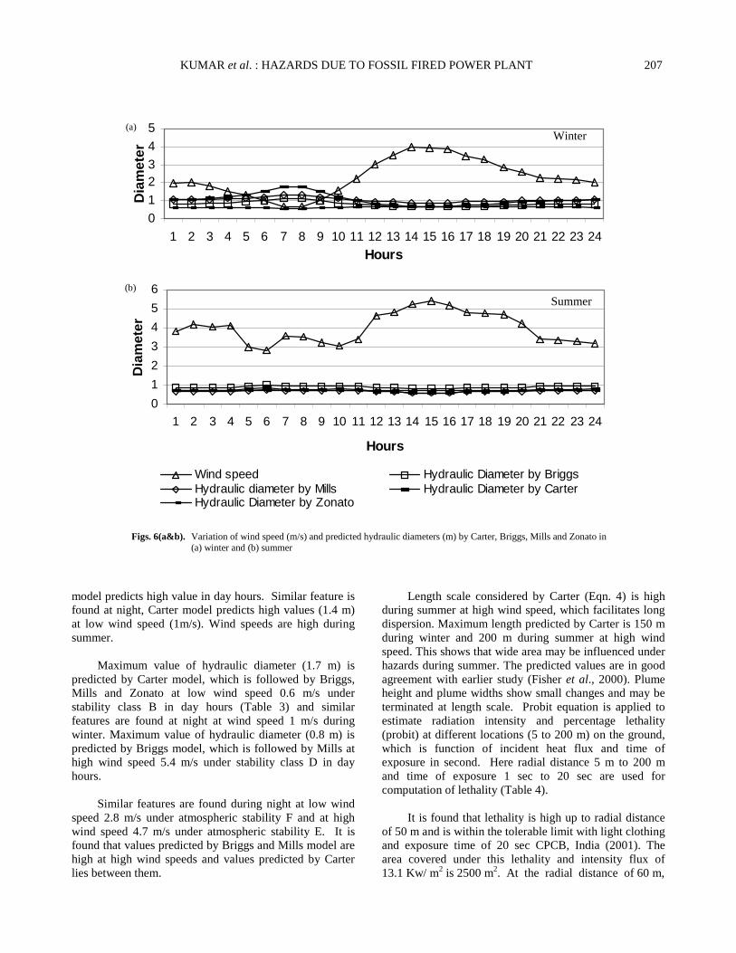
Figs. 6(a&b). Variation of wind speed (m/s) and predicted hydraulic diameters (m) by Carter, Briggs, Mills and Zonato in (a) winter and (b) summer

model predicts high value in day hours. Similar feature is found at night, Carter model predicts high values (1.4 m) at low wind speed (1m/s). Wind speeds are high during summer.

Maximum value of hydraulic diameter (1.7 m) is

predicted by Carter model, which is followed by Briggs, Mills and Zonato at low wind speed 0.6 m/s under stability class B in day hours (Table 3) and similar features are found at night at wind speed 1 m/s during winter. Maximum value of hydraulic diameter (0.8 m) is predicted by Briggs model, which is followed by Mills at high wind speed 5.4 m/s under stability class D in day hours.

Similar features are found during night at low wind speed 2.8 m/s under atmospheric stability F and at high wind speed 4.7 m/s under atmospheric stability E. It is found that values predicted by Briggs and Mills model are high at high wind speeds and values predicted by Carter lies between them.

Length scale considered by Carter (Eqn. 4) is high during summer at high wind speed, which facilitates long dispersion. Maximum length predicted by Carter is 150 m during winter and 200 m during summer at high wind speed. This shows that wide area may be influenced under hazards during summer. The predicted values are in good agreement with earlier study (Fisher et al., 2000). Plume height and plume widths show small changes and may be terminated at length scale. Probit equation is applied to estimate radiation intensity and percentage lethality (probit) at different locations (5 to 200 m) on the ground, which is function of incident heat flux and time of exposure in second. Here radial distance 5 m to 200 m and time of exposure 1 sec to 20 sec are used for computation of lethality (Table 4).

It is found that lethality is high up to radial distance of 50 m and is within the tolerable limit with light clothing and exposure time of 20 sec CPCB, India (2001). The area covered under this lethality and intensity flux of 13.1 Kw/ m2 is 2500 m2. At the radial distance of 60 m,

0

1

23

4

5

1 2 3 4 5 6 7 8 9 10 11 12 13 14 15 16 17 18 19 20 21 22 23 24

Hours

Dia

met

er

0

1

2

3

4

5

6

1 2 3 4 5 6 7 8 9 10 11 12 13 14 15 16 17 18 19 20 21 22 23 24

Hours

Dia

met

er

Wind speed Hydraulic Diameter by BriggsHydraulic diameter by Mills Hydraulic Diameter by CarterHydraulic Diameter by Zonato

Winter

Summer

(a)

(b)

208 MAUSAM, 60, 2 (April 2009)

TABLE 4

Estimation of Lethality doses of thermal radiation

Radial distance (m)

Time of Exposure (s)

Lethality Radiation (KWm-2)

Area (m2)

5 20 41.4 1312.5 78.5

10 20 30.5 328.1 314.2

15 20 24.1 145.8 706.9

20 20 19.6 82.0 1256.8

25 20 16.1 52.5 1963.7

30 20 13.2 36.4 2827.8

35 20 10.8 26.7 3848.9

40 20 8.7 20.5 5027.2

45 20 6.9 16.2 6362.5

50 20 5.2 13.1 7855.0

60 20 2.4 9.1 11311.2

70 20 < 0.1 6.6 15395.8

lethality is 2.4 for exposure time 20 second with any cover, which decreases considerably at 70 m and beyond. This shows that distance beyond the radial distance of 70 m at exposure time 20 sec is safe under hazardous condition. 5. Conclusions

In this study, hazards associated with a fuel-based

power plant located in coastal Gujarat are assessed using four pool fire models namely Carter, Briggs, Mill and Zonato. This assessment includes fuel tank details (tank capacity, calorific value and heat rate of fuel), model input parameters and observed meteorological conditions during winter and summer. The results of this study are summarized below : (i) It is observed that lateral and vertical spread, plume widths, heights and hydraulic diameter are high at low wind speeds in winter. Wind speed increases in summer, low values are noted. Dispersion dominates over buoyancy and consequently length scales are large. Results show that wide areas of habitation and human settlement at northeast of the site may be under potentially hazardous conditions in summer.

(ii) Comparison of model results shows that Carter model predicts maximum values of plume spread, width, height and hydraulic diameter, which are followed by those of Briggs, Mills and Zonato at low wind speed. As the wind speed increases, Briggs model predicts maximum values, followed by those of Carter, Mills and Zonato models. Also predicted values are found to be high at low wind speed in the morning or late night and low around noon at high wind speed. (iii) Lethality of 2.4 % under thermal radiation (1.0 W Kg-1m-2) on human settlement at radial distance of 70 m and beyond from the source is within the tolerable limit with exposure of 20 sec. Length scale predicted by Carter model is high during summer which facilitates long dispersion at high wind speed, These results are encouraging for studying the impact of local meteorology on risk and plume behaviour due to pool fire at different coastal sites in India. Acknowledgments

Meteorological data used in the study have been obtained from the India Meteorological Department.


References

Atkinson, G. T. and Jagger, S. F., 1992, “Exposure of organophosphorus pesticides to turbulent diffusion flames”, Journal of Loss Prevention Process in Industry, 5, 271-277.

Bennett, M., Sutton, S. and Gardiner, D. R. C., 1992, “An Analysis of lidar measurement of buoyant plume rise and dispersion at five power stations”, Atmospheric Environment, 26A, 3249-3263.

Bennett, M., 1995, “A lidar study of the limits to buoyancy plume rise in a well-mixed boundary layer”, Atmospheric Environment, 29, 2275 - 2288.

Carruthers, D. J., Mckeown, A. M., Hall, D. J. and Porter, S., 1999, “Validation of ADMS against wind tunnel data of dispersion from chemical ware house fires”, Atmospheric Environment, 33, 1937-1953.

Carter, D. A., 1989, “Methods for estimating the dispersion of toxic combustion products from large fires”, Chemical Engineering Research Design, 67, 348-352.

Central Pollution Control Board, India, 1997, “Assessment of Impact to Air Environment : Guide line to conducting Air Quality Modelling”, PROBES 70.

Central Pollution Control Board, India, 2001, Hazardous Waste Management Series: HAZWAMS/16/2000-01.

Clarke, R. H., 1979, “A model for short and medium range dispersion of radionuclide released to the atmosphere”, Report NRPB-R91, National Radiological Protection Board.

Fisher, B. E. A., Metcalfe, E. I., Vince, I. and Yates, A., 2000, “Modelling Plume rise and dispersion from pool fires”, Atmospheric Environment, 35, 2101-2110.

Ghoniem, F. Ahmed, Zhang Xiaoming, Knio Omar, Baum R. Howard and Rehm, Renald, G., 1993, “Dispersion and deposition of smoke plumes generated in massive fires”, 33, 275-293.

Hall, D. J., Walker, V., S. and Marsland, G. W., 1995, “Plume dispersion from chemical ware house fires”, BRE Client Report CR56/95 prepared for the European Commission on STEP project no. CT 90-0096, for the Toxic Substance Division, Department of Environment.

Hunt, J. C. R. and Weber, A. H., 1979, “A Lagrangian statistical analysis of diffusion from ground-level source in a turbulent boundary layer”, Quarterly Journal of Royal Meteorological Society, 105, 423-443.

Jones, J. A., 1983, “Models to allow for the effects of coastal sites, plume rise and building dispersion of radio nuclides and guidance on the value of deposition velocity and washout coefficients”, NRPB Report R157.

Mills, M. T., 1987, “Modeling the release and dispersion of toxic combustion products from pool fires”, Paper from international conference on vapor cloud modeling, Cambridge, MA, USA, 2-4.11.1987.

Moore, D. J., 1974, “A comparison of the trajectory of rising buoyancy plumes with theoretical/empirical models”, Atmospheric Environment, 8, 441-457.

Moore, D. J., 1980, “Lecture on plume rise”, In; Longhetto, A.(Ed.), Atmospheric Planetary Boundary Layer Physics Developments in Atmospheric Science, Vol. I, Elsevier, Amsterdam, 327-354.

Zonato, C., Vidil, A., Patorino, R. and De Faveri, D. M., 1993, “Plume rise of smoke coming from burning fires”, J. of Hazards materials, 34, 69-79.

Appendix Nomenclature a,b,c,d empirical coefficients, dimensionless cp specific heat capacity of pool fire, KJkg-1 K-1

D effective tank diameter, m FB buoyancy flux, m4s– 3

g acceleration due to gravity, ms-2

Hzo plume centerline height (Zonato equation), m HB plume centerline height (Briggs equation), m Hca plume centerline height (Carter equation), m HM plume centerline height (Mills equation), m QE effective hest release rate, KJs-1

QH total pool fire heat release rate, KJs-1

Ta ambient temperature K u10m wind speed at 10 m altitude, ms-1

X down wind distance from centre of fire, m

210 MAUSAM, 60, 2 (April 2009)

Greek letters β entrainment coefficient (conventionally = 0.6), dimensionless Γ potential temperature gradient, K (100 m)-1

ε fraction of radiant emission to environment, dimensionless ρ density of air, Kg m-3

σy lateral plume dispersion coefficient, m, dimensionless σz vertical plume dispersion coefficient, m, dimensionless

Assessment of scale of hazards due to pool fire for a...

Documents

Transcript of Assessment of scale of hazards due to pool fire for a...