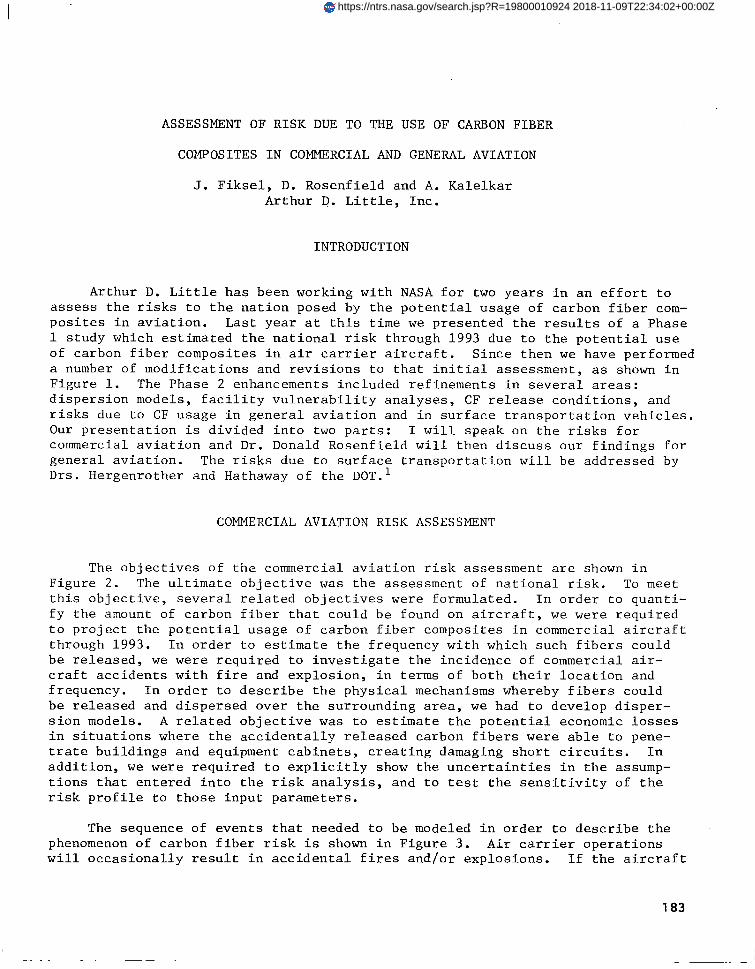
ASSESSMENT OF RISK DDE TO THE USE OF CARBON FIBER

COMPOSITES IN COMMERCIAL AND GENERAL AVIATION

J. Fiksel, D. Rosenfield and A. Kalelkar Arthur D. Little, Inc.

INTRODUCTION

Arthur D. Little has been working with NASA for two years in an effort to assess the risks to the nation posed by the potential usage of carbon fiber com- posites in aviation. Last year at this time we presented the results of a Phase 1 study which estimated the national risk through 1993 due to the potential use of carbon fiber composites in air carrier aircraft. Since then we have performed a number of modifications and revisions to that initial assessment, as shown in Figure 1. The Phase 2 enhancements included refinements in several areas: dispersion models, facility vulnerability analyses, CF release conditions, and risks due to CF usage in general aviation and in surface transportation vehicles. Our presentation is divided into two parts: I will speak on the risks for commercial aviation and Dr. Donald Rosenfield will then discuss our findings for general aviation. The risks due to surface transportation will be addressed by Drs. Hergenrother and Hathaway of the D0T.l

COMMERCIAL AVIATION RISK ASSESSMENT

The objectives of the commercial aviation risk assessment are shown in Figure 2. The ultimate objective was the assessment of national risk. To meet this objective, several related objectives were formulated. In order to quanti- fy the amount of carbon fiber that could be found on aircraft, we were required to project the potential usage of carbon fiber composites in commercial aircraft through 1993. In order to estimate the frequency with which such fibers could be released, we were required to investigate the incidence of commercial air- craft accidents with fire and explosion, in terms of both their location and frequency. In order to describe the physical mechanisms whereby fibers could be released and dispersed over the surrounding area, we had to develop disper- sion models. A related objective was to estimate the potential economic losses in situations where the accidentally released carbon fibers were able to pene- trate buildings and equipment cabinets, creating damaging short circuits. In addition, we were required to explicitly show the uncertainties in the assump- tions that entered into the risk analysis, and to test the sensitivity of the risk profile to those input parameters.

The sequence of events that needed to be modeled in order to describe the phenomenon of carbon fiber risk is shown in Figure 3. Air carrier operations will occasionally result in accidental fires and/or explosions. If the aircraft

183

https://ntrs.nasa.gov/search.jsp?R=19800010924 2018-11-09T22:34:02+00:00Z

is carrying carbon fiber composites in the structure, then some of these fibers may be burned away by an intense fire, will rise in the convection plume and will be dispersed over a large area, depending upon the atmospheric conditions and the wind direction. If there are buildings or other facilities located in the path of the carbon fiber cloud, and if these buildings contain electronic equipment which is potentially vulnerable to the fibers, then there is a possi- bility that they will penetrate these buildings, damage the equipment and thus result in economic losses to the residents or proprietors of these facilities. We will separately address each of the steps involved in this sequence of events and show how we analyzed them.

Carbon Fiber Usage

In order to describe the usage of carbon fiber composites in aircraft, we divided the commercial aircraft into three categories of jets--small, medium and large jets. Each of the jet aircraft produced by the major airframe manu- facturers was assigned to one of these classes. We did not consider other classes of aircraft,such as turbo-props,since there is not expected to be a great deal of carbon fiber usage for these type of aircraft. The projections for carbon fiber usage in commercial aircraft are shown in Figure 4. These are based on estimates obtained from the three major U.S. airframe manufacturers, McDonnell Douglas, Lockheed and Boeing. They estimated both the fleet mix, that is the relative numbers of different sizes of aircraft in service in 1993, and the potential usage of carbon fiber composites for each of these classes. As indicated in Figure 4, roughly half of the aircraft in service in 1993 will be large jets, the majority of which will be using carbon fiber composites. The projected weight of actual carbon fibers, including the epoxy binding,ranges from only 11 kg. on some of the small aircraft to as much as 15 600 kg. on some of the large aircraft. For the purposes of the risk analysis we used these es- timated ranges to develop a probability distribution for the amount of carbon fiber involved in an aircraft accident.

To characterize air carrier activity within the U.S. as a whole, we focused upon the 26 large hub airports which account for approximately 70% of domestic passenger enplanements. As shown in Figure 5, the balance of the passenger traffic in the U.S. is accounted for by 40 medium hub airports and a large num- ber of small hub airports. Only about 3% of total commercial passenger enplane- ments occur at airports other than these hub airports designated by the F.A.A. Our approach was to study in detail the traffic patterns and the exposed popu- lation in the vicinity of the 26 large hubs and then to extrapolate the result- ing risk estimates to the rest of the nation.

Accident Conditions

The typical conditions surrounding a severe fire and/or explosion in the case of an air carrier accident were investigated through use of the National Transportation Safety Board accident and incident statistics for the years 1968- 1976. Using their records, we created a data base of aircraft accidents that listed for each accident the phase of operation, the location of the accident, the weather conditions at the time of the accident, the nature of the fire, and

184

other relevant details. This data base was augmented with the help of the air- frame manufacturers who provided additional data on accident characteristics, such as fire duration, that would affect carbon fiber release conditions. We then utilized these data to determine the distribution of possible accident char- acteristics. We found that almost half of the severe accidents involving fire occurred during the landing phase. As shown in Figure 6, the take-off phase ac- counts for one-quarter of these accidents, with the remainder being distributed in either the static/taxi or cruise phase. Cruise accidents were dealt with through a separate analysis since the location of these accidents is essentially random. However, the static, take-off or landing accidents were all associated with specific airport locations.

From an analysis of the location of accidents relative to airport runways, we found that over 80% of accidents occur within 10 kilometers of the airport, and in fact 60% of accidents occur at the airport. We also investigated the angle between the accident location and the line of the runway to establish more precisely the potential locations of such accidents.

Historically, there have been about 3.8 accidents per year involving jet air carriers. Alt:hough air carrier operations are gradually.increasing in num- ber, the accident frequency appears to be relatively constant from year to year. Therefore, we did not project any increase in accidents through 1993. Based on the expected fraction of the air carrier fleet that would be carrying carbon fiber in 1993, the projected frequency of incidents involving fire on aircraft carrying composites of carbon fibers would be approximately 2.7 per year in 1993.

Release and Dispersion

There are two different types of scenarios that describe possible carbon fiber release situations in the aftermath of an air carrier incident. One of them is a simple fire plume in which the fibers are carried aloft by the plume and then dispersed. The second is the fire and explosion case in which there is a sudden rapid conflagration of fuel resembling an explosion, in which much more rapid burning of composite and a sudden release of fibers can take place over a short period of time. Based on the 92 accident data base compiled by the airframe manufacturers, we estimated conservatively that at most 5% of air car- rier accidents would result in explosive release of carbon fibers of the type described.

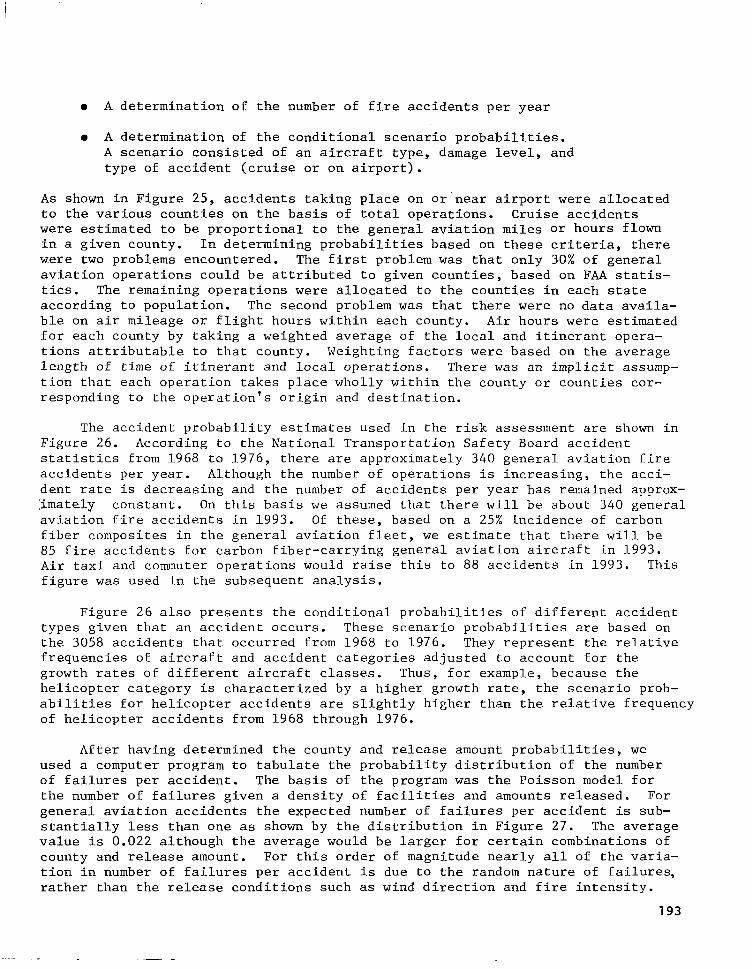
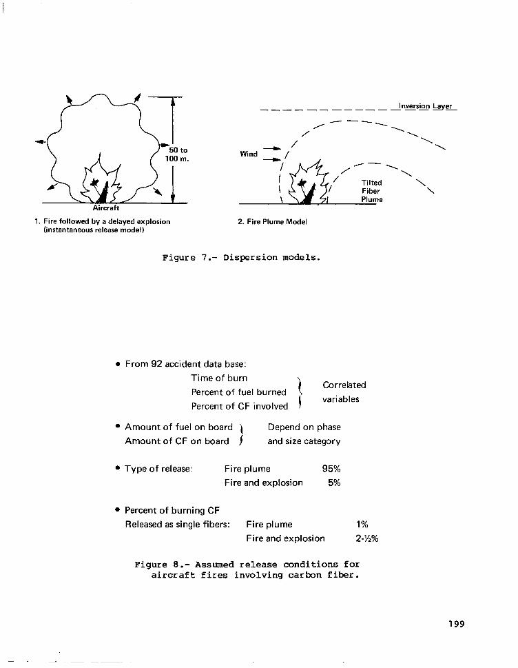
The two dispersion models corresponding to the two accident and carbon fi- ber release scenarios are shown graphically in Figure 7. In the fire and explo- sion case, we consider only those accidents in which there was a delayed explo- sion preceded by a period of burn during which the epoxy or resin surrounding the fibers would be burned away. This would expose the carbon fibers to an agitation by the force of the conflagration and thus would hypothetically result in a larger number of single fibers released. This scenario was modeled as an instantaneous release in the form of a cloud at a height of 10 meters above the site of the accident. In the fire plume model, rather than having an instanta- neous release,we have a continuous release of fibers over the period that the aircraft burns. The carbon fiber plume rises until it meets the inversion layer

185

and then is tilted or reflected back toward the ground. The direction and velocity of the wind determine the exposure contour over which carbon fibers will be deposited.

The extent of dispersion of carbon fibers from a burning aircraft and the level of resulting exposures to the surrounding area are greatly influenced by the release conditions at the time of the accident. Release conditions include the weather conditions, such as atmospheric stability class, wind velocity and wind direction. These were examined at each of the 26 major airports with the help of NOAA statistics. However, it was more difficult to estimate the release conditions associated with the duration and the intensity of the fire. With the help of the 92 accident data base compiled by the airframe manufacturers we were able to develop distributions for several of the important release variables, as shown in Figure 8. These included the time of burn--that is, the duration over which the fire lasted, the percent of fuel burned,and the percent of carbon fi-. ber involved. Our approach to estimating CF involvement is described below. The degree of carbon fiber involvement was correlated with both the duration of the fire and the percent of fuel burned. Roughly speaking, the greater the amount of fuel burned, the longer the duration of the burn, and the greater the potential carbon fiber involvement. In addition, the amount of fuel on board was estimated for different phases of operation and different aircraft size cate- gories, and the amount of carbon fibers on board was estimated for the three size classes of aircraft. This allowed calculation of the actual amount of fuel burned and the actual amount of carbon fiber involved.

Even though an aircraft may be carrying over 15 000 kg. of CF composite, the amount of carbon fibers that could be released in a fire is significantly less, partly because of the fact that not all the carbon fibers can be released as single fibers in a burn, and partly because the entire aircraft structure will not necessarily be involved in the fire.

Based on experimental findings, which were described by Dr. Vernon Be11,'it is estimated that not more than 1% of the carbon fibers would be released in most fire plumes, and that not more than 2.5% would be released in most fire and explosion scenarios. These are conservative estimates using the best judgment and interpretation of the experiments conducted by NASA and other groups on burning composite materials.

To examine structure involvement, we used the results of an analysis by the airframe manufacturers, who estimated the amount of structure that could be involved in a fire for various components of their aircraft. Using the data base of 92 fire incidents, they estimated the percent of each component that was involved in the fire, thus creating a distribution of potential structural in- volvement. As shown in Figure 9, we combined the structural damage estimates with the projected usage of carbon fibers by component (also developed by the airframe manufacturers) to produce estimates of the potential carbon fiber in- volvement in air carrier fires. The range of involvement varied from zero, reflecting a fire which did not damage any of the structure containing carbon fibers, to 100% involvement in which all portions of the aircraft containing CF were completely involved in the fire. Our median estimates of carbon fiber involvement were 45% for small jets, 69% for medium jets, and 64% for large jets. This variation is due largely to the different levels of CF usage in the different aircraft size classes.

186

Exposure Contours and Demographics

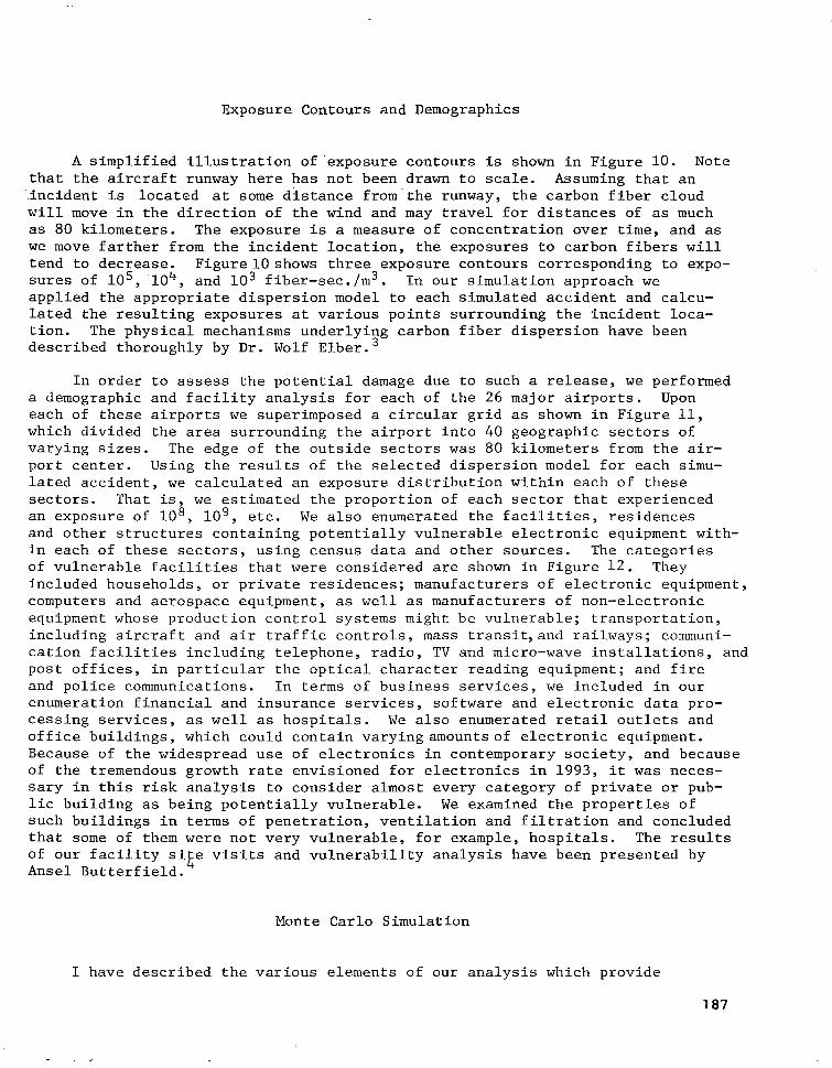
A simplified illustration of'exposure contours is shown in Figure 10. Note that the aircraft runway here has not been drawn to scale. Assuming that an

Iincident is located at some distance from.the runway, the carbon fiber cloud will move in the direction of the wind and may travel for distances of as much as 80 kilometers. The exposure is a measure of concentration over time, and as we move farther from the incident location, the exposures to carbon fibers will tend to decrease. Figure10 shows three exposure contours corresponding to expo- sures of 105, 104, and lo3 fiber-sec./m3. In our simulation approach we applied the appropriate dispersion model to each simulated accident and calcu- lated the resulting exposures at various points surrounding the incident loca- tion. The physical mechanisms underlying carbon fiber dispersion have been described thoroughly by Dr. Wolf Elber.3

In order to assess the potential damage due to such a release, we performed a demographic and facility analysis for each of the 26 major airports. Upon each of these airports we superimposed a circular grid as shown in Figure 11, which divided the area surrounding the airport into 40 geographic sectors of varying sizes. The edge of the outside sectors was 80 kilometers from the air- port center. Using the results of the selected dispersion model for each simu- lated accident, we calculated an exposure distribution within each of these sectors. That is, we estimated the proportion of each sector that experienced an exposure of lo*, log, etc. We also enumerated the facilities, residences and other structures containing potentially vulnerable electronic equipment with- in each of these sectors, using census data and other sources. The categories of vulnerable facilities that were considered are shown in Figure 12. They included households, or private residences; manufacturers of electronic equipment, computers and aerospace equipment, as well as manufacturers of non-electronic equipment whose production control systems might be vulnerable; transportation, including aircraft and air traffic controls, mass transit,and railways; communi- cation facilities including telephone, radio, TV and micro-wave installations, and post offices, in particular the optical character reading equipment; and fire and police communications. In terms of business services, we included in our enumeration financial and insurance services, software and electronic data pro- cessing services, as well as hospitals. We also enumerated retail outlets and office buildings, which could contain varying amounts of electronic equipment. Because of the widespread use of electronics in contemporary society, and because of the tremendous growth rate envisioned for electronics in 1993, it was neces- sary in this risk analysis to consider almost every category of private or pub- lic building as being potentially vulnerable. We examined the properties of such buildings in terms of penetration, ventilation and filtration and concluded that some of them were not very vulnerable, for example, hospitals. The results of our facility site visits and vulnerability analysis have been presented by Ansel Butterfield.4

Monte Carlo Simulation

I have described the various elements of our analysis which provide

187

the necessary inputs for a Monte Carlo simulation. These data inputs included the accident characteristics, the release conditions, the dispersion model, and the characteristics of vulnerable facilities. Once these elements had been assembled, we performed a Monte Carlo simulation of potential aircraft accidents at each of the 26 large hub airports. We used the Monte Carlo method to develop an individual risk profile for each airport,and then these risk profiles were combined into a national risk profile. (A risk profile is a graph indicating the probability of exceeding various levels of dollar loss.) Figure 13 shows the Monte Carlo procedure for an individual airport. Each point at which a question mark is shown denotes a random draw from an input distribution. These distributions were developed through the analyses discussed previously.

The Monte Carlo procedure works in the following manner: It simulates a large number of accidents, on the order of hundreds or thousands of accidents, and for each one draws from probability distributions a set of conditions for that accident. By repeating the simulation many times, we show the full range of possible accident types and thus develop a distribution of the potential accident results. As shown in Figure 13, the aircraft and incident details, such as the size of the plane and the phase of the operation,are randomly drawn, and these in turn influence the probable accident location, the likelihood of a delayed explosion, and the assumed release conditions.

If an explosion does occur, which happens about 5% of the time, then the fire and explosion model is selected, whereas if it does not occur, the fire plume model is selected to compute exposures. The weather conditions such as stability class and wind velocity are drawn from weather distributions for the particular airport in question,and these together with the release conditions determine the exposures resulting from the dispersion model. These exposures are then calculated at a large number of points within the 40-sector grid and an exposure distribution is found for each sector. From this exposure distribution we use the penetration and vulnerability characteristics of the facilities ex- posed, and an economic analysis model which estimates the economic losses result- ing for each affected facility. The losses are then summed to determine the total economic losses resulting from the simulated accident. Once this is com- plete, the computer returns and simulates another accident, drawing a new set of aircraft/incident details. This procedure was repeated iteratively until enough samples had been taken to get a reasonably accurate distribution of the economic losses resulting from an accident. In this way we developed 26 individual risk profiles for the large hub airports.

An example of the outcome of a typical computer simulation is shown in Figure 14. In this case, the computer generated a hypothetical accident at La Guardia airport, relatively close to the center of a runway. The aircraft in- volved was a medium jet in a static or taxi phase, which somehow caught fire. About 8500 kg. of fuel were burned over a period of more than thirty minutes, releasing 22 kg. of carbon fibers. There was also a delayed explosion during the burn. Based upon the randomly drawn weather conditions, the CF cloud moved westward, toward New York City, creating exposures as high as lOa fiber-seconds per cubic meter at the airport, and lo7 fiber-sec./m3 within 3 km. of the air- port. The resulting losses due to equipment failures amounted to a total of $178, of which households accounted for $66. By performing hundreds of itera- tions like this one, the computer generated a risk profile for La Guardia air- port.

188

The next task was to derive the national risk profile. This was done by combining the individual risk profiles with information concerning potential losses due to cruise accidents and accidents at airports other than the 26 considered.

Risk Profile Development

We developed two kinds of national risk profiles in this analysis. One of them was the risk profile for a single incident, which gave the distribution of dollar losses resulting from any one air carrier accident. This was derived by taking a weighted mixture of the individual airport risk profiles for a single incident, weighted by the frequency of incidents at each airport. This proced- ure is shown in Figure 15. The second type of national risk profile derived was the national annual risk profile which showed the distribution of total losses due to accidents involving carbon fibers. This annual risk profile incorporates the possibility of one, two, three or more accidents involving carbon fiber re- lease during any given year. To derive the annual risk profile we used the national risk profile for a single incident and performed a convolution proced- ure based on the annual frequency of such accidents.

Before proceeding to the results of the risk analysis, it is important to note the major assumptions that entered into this analysis. The most important assumptions are listed in Figure 16. First, atmospheric conditions are assumed to remain constant during the dispersion of the carbon fiber cloud. This is a somewhat unrealistic assumption since weather conditions are constantly changing, and a cloud moving at a rate of a few kilometers per hour could take as much as a day to cover 80 kilometers. However, it would be too complex to simulate dif- ferent atmospheric conditions in different geographic sectors, and therefore this assumption was made. The assumption is not expected to introduce any bias into the risk analysis since the variation of atmospheric conditions will some- times increase and sometimes decrease the resulting exposures. We also assumed that there was no precipitation, which is a conservative assumption since if pre- cipitation does occur it may wash out some of the fibers, resulting in lower airborne exposures on the ground. It was found that there was a high likelihood of rain or other forms of precipitation being associated with an aircraft acci- dent, since many of the accidents in the historical data base occurred in IFR, or instrument flight rules weather. The second major assumption is that for a given facility category all facilities are equal in size, equipment inventory, and financial characteristics. Again this is a necessary assumption due to the enormous volume of data that would have to be processed in order to identify all the different sizes or scales of facilities that do exist. Instead, we took the average case, based upon regional statistics for each facility category, and at- tempted to model the typical vulnerable facility. The variation in facility characteristics would introduce a little more variation into the risk profile but should not affect the results too greatly because of the large number of facilities involved that would tend to average each other out. The third major assumption is that all equipment is activated and that failures occur immediately after exposure. This assumes, first of all,that equipment which is exposed is in an activated state and is vulnerable to the fibers at the time of exposure. Since some fraction of the eletronic equipment exposed will not be activated,

189

this tends to be a conservative assumption. On,the other hand, there is a phen- omenon of post-exposure vulnerability, in which fibers that are deposited upon equipment do not cause a problem immediately but will affect the equipment when it is turned on at a later date. This phenomenon was not modeled explicitly, but it is taken into account by assuming continuous activation and failures im- mediately after exposure.

The annual risk profile for economic losses due to air carrier fires in- volving carbon fibers is shown in Figure 17. The horizontal axis shows the total economic losses in dollars as a result of carbon fiber accidents during a given year. The vertical axis shows the annual probability of exceeding each dollar loss value. For example, an annual loss of approximately one thousand dollars would be exceeded with a probability of 10-l, in other words once every ten years. An annual loss of ten thousand dollars would be exceeded about once every three hundred years. The expected annual losses due to CF released from air carrier fires in 1993 is about $470. This includes only those losses in- curred by failures of equipment in the civilian sector.

Discussion of Results

The confidence bounds on the risk profile show the sensitivity of the risk estimates to variations in the input parameters. These confidence bounds are based upon several different sources of uncertainty: the statistical error due to the simulation method, the statistical error in estimation of accident fre- quency , and the modeling errors due to uncertainty about input parameters. The former two sources of uncertainty were judged to contribute less than an order of magnitude to the confidence bound at the high-loss extreme, and considerably less than that at average loss values. The confidence bounds are wider at high loss values because the simulation may not turn up an extremely unlikely high- loss event even among thousands of simulated events.

To estimate the modeling errors, we performed a sensitivity analysis by varying several of the key input parameters. The results are shown in Figure 18. This analysis was run on the individual airport risk profile which had the high- est mean loss of the 26 hubs, namely Detroit. Of the three parameters tested, the largest increase in risk was obtained by setting the composite on the air- craft at its highest possible value, 15.652 kg. This increased the mean loss per incident by a factor of about 7, and increased the standard deviation and maximum value of the losses by a factor of about 4.5. Restricting the simula- tion model to only explosive releases increased these statistics by a factor of 2 or 3, while setting the atmospheric stability class to E (moderately stable weather) increased the loss distribution only slightly. The two latter condi- tions are those which tend to result in highest exposures downwind of the release point. We concluded that modeling errors contributed less than an order of magnitude to the uncertainty of the risk profile.

As a final verification of the simulation results, we compared the national conditional profile for dollar losses per incident against a risk profile ob- tained through an alternative analytic approach. The latter approach, which is based upon a Poisson model of equipment failures, will be described by Dr.

190

Rosenfield in the context of the general aviation risk assessment. As shown in Figure 19, the two methods agreed fairly well, with their mean values differing by a factor of less than 3. The simulation indicated an average loss of $172 per incident, while the Poisson method resulted in an average loss of $472 per incident.

GENERAL AVIATION RISK ASSESSMENT

This section reports on the investigation of the effects of carbon fiber usage in general aviation aircraft. The objective of this analysis was to as- sess the national risk through 1993 in terms of economic losses and to deter- mine the sensitivity of the risk assessment to uncertainties in the input data. In formulating this objective, we identified as sub-objectives the projection of potential usage of carbon fiber composites in general aviation aircraft through 1993 and the investigation of fire accidents in general aviation with- in the U.S. The risk assessment thus involved forecasting future carbon fiber usage, development of an accident model for general aviation aircraft, analysis of the possible release amounts in general aviation accidents, and assessment of the economic consequences of a given release. These objectives are summarized in Figure 20.

Methodology Overview

The methodology utilized for the general aviation risk assessment was quite different from that utilized for commercial aviation. The major issues involved in selecting a methodology are summarized in Figure 21. The simula- tion model is more appropriate for large releases which will result in large numbers of failures, and allows detailed identification of the geographic dis- tribution of facilities as well as of the different possible accident and release conditions. As noted previously, the simulation approach results in statistical uncertainty at the high-loss tail of the risk profile. In the case of general aviation, the number of failures per incident was expected to be ex- tremely small, and the dominant variation in economic losses appeared to be caused by the random failure process rather than by the variations in physical conditions. Furthermore, there were insufficient data available to allow a detailed modeling of release and dispersion scenarios.

For these reasons, an analytic methodology was developed to synthesize the accident model and carbon fiber usage forecast for assessment of the eco- nomic consequences of accidents. This methodology is shown in Figure 22. There were two key parameters influencing the economic consequences of accidents. The first was the amount of fibers released in an accident. By examining the dif- ferent types of general aviation aircraft and their accident statistics, a distribution of amounts of carbon fibers potentially released in accidents was developed. The second key parameter was the density of facilities near the location of an accident. Thus, an important aspect of the accident model was a quantitative description of the distribution of facility densities. The 3,000 counties in the United States were chosen as a basis for estimating facility density, and hence a methodology was developed to apportion accidents

191

to the various counties. After a range of county and release amounts was de- veloped, the distribution of failures given an aviation accident was determined. A Poisson probability model was developed for this purpose and a computer pro- gram was utilized to tabulate failure probabilities as a function of the amount released and the county, and to aggregate these into a national risk profile of dollar losses. Based on the distribution of the number of equipment failures per accident, the statistics of dollar losses per accident, and the number of accidents per year, expressions were developed for the mean and standard devia- tion of a dollar loss per year. From these statistics, approximations and bounds were developed for the probability distribution of annual economic losses.

Before examining the details of this methodology it is important to under- stand the theoretical basis of the Poisson approach, as depicted in Figure 23. For a given release scenario and equipment type, the number of equipment fail- ures may be approximated by a Poisson distribution with mean No. The mean number of failures is given by integrating the equipment density over the area in question and multiplying by the equipment failure probability, which is nearly linear in E for low values of the exposure E. Now, provided the amount released is held constant, we can aggregate over many release scenarios, and show that the average No is proportional to the surface integral S of the expo- sure, which in turn may be shown to depend only on the amount released. Thus an expression is obtained for the mean number of failures per incident in terms of just the average facility density, the amount of CF released, and the equip- ment vulnerability. This enables us to assess the risk without requiring de- tailed data on accident conditions or geographic locations.

Steps in Risk Analysis

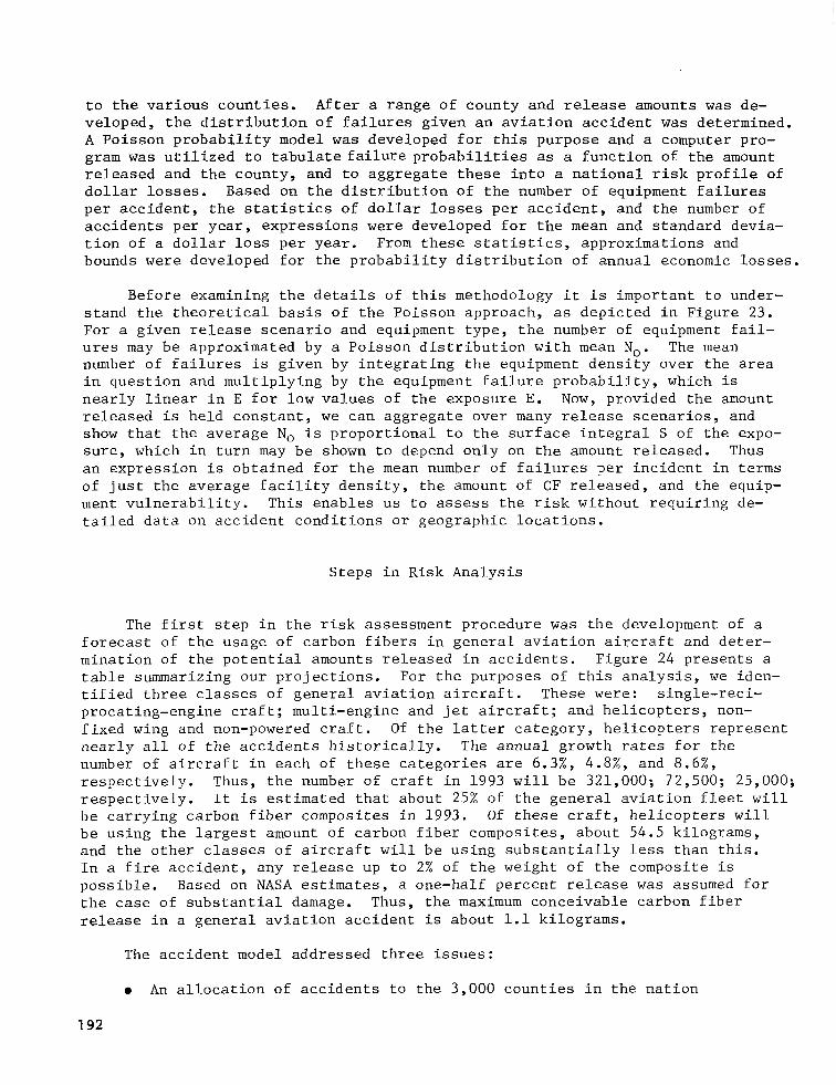
The first step in the risk assessment procedure was the development of a forecast of the usage of carbon fibers in general aviation aircraft and deter- mination of the potential amounts released in accidents. Figure 24 presents a table summarizing our projections. For the purposes of this analysis, we iden- tified three classes of general aviation aircraft. These were: single-reci- procating-engine craft; multi-engine and jet aircraft; and helicopters, non- fixed wing and non-powered craft. Of the latter category, helicopters represent nearly all of the accidents historically. The annual growth rates for the number of aircraft in each of these categories are 6.3%, 4.8%, and 8.6%, respectively. Thus, the number of craft in 1993 will be 321,000; 72,500; 25,000; respectively. It is estimated that about 25% of the general aviation fleet will be carrying carbon fiber composites in 1993. Of these craft, helicopters will be using the largest amount of carbon fiber composites, about 54.5 kilograms, and the other classes of aircraft will be using substantially less than this. In a fire accident, any release up to 2% of the weight of the composite is possible. Based on NASA estimates, a one-half percent release was assumed for the case of substantial damage. Thus, the maximum conceivable carbon fiber release in a general aviation accident is about 1.1 kilograms.

The accident model addressed three issues:

l An allocation of accidents to the 3,000 counties in the nation

192

l A determination of the number of fire accidents per year

l A determination of the conditional scenario probabilities. A scenario consisted of an aircraft type, damage level, and type of accident (cruise or on airport).

As shown in Figure 25, accidents taking place on or near airport were allocated to the various counties on the basis of total operations. Cruise accidents were estimated to be proportional to the general aviation miles or hours flown in a given county. In determining probabilities based on these criteria, there were two problems encountered. The first problem was that only 30% of general aviation operations could be attributed to given counties, based on FAA statis- tics. The remaining operations were allocated to the counties in each state according to population. The second problem was that there were no data availa- ble on air mileage or flight hours within each county. Air hours were estimated for each county by taking a weighted average of the local and itinerant opera- tions attributable to that county. Weighting factors were based on the average length of time of itinerant and local operations. There was an implicit assump- tion that each operation takes place wholly within the county or counties cor- responding to the operation's origin and destination.

The accident probability estimates used in the risk assessment are shown in Figure 26. According to the National Transportation Safety Board accident statistics from 1968 to 1976, there are approximately 340 general aviation fire accidents per year. Although the number of operations is increasing, the acci- dent rate is decreasing and the number of accidents per year has remained approx- :imately constant. On this basis we assumed that there will be about 340 general aviation fire accidents in 1993. Of these, based on a 25% incidence of carbon fiber composites in the general aviation fleet, we estimate that there will be 85 fire accidents for carbon fiber-carrying general aviation aircraft in 1993. Air taxi and commuter operations would raise this to 88 accidents in 1993. This figure was used in the subsequent analysis.

Figure 26 also presents the conditional probabilities of different accident types given that an accident occurs. These scenario probabilities are based on the 3058 accidents that occurred from 1968 to 1976. They represent the relative frequencies of aircraft and accident categories adjusted to account for the growth rates of different aircraft classes. Thus, for example, because the helicopter category is characterized by a higher growth rate, the scenario prob- abilities for helicopter accidents are slightly higher than the relative frequency of helicopter accidents from 1968 through 1976.

After having determined the county and release amount probabilities, we used a computer program to tabulate the probability distribution of the number of failures per accident. The basis of the program was the Poisson model for the number of failures given a density of facilities and amounts released. For general aviation accidents the expected number of failures per accident is sub- stantially less than one as shown by the distribution in Figure 27. The average value is 0.022 although the average would be larger for certain combinations of county and release amount. For this order of magnitude nearly all of the varia- tion in number of failures per accident is due to the random nature of failures, rather than the release conditions such as wind direction and fire intensity.

193

As mentioned earlier, the expected number of equipment failures is thus propor- tional to the density of facilities and the amount of carbon fibers released, and inversely proportional to the mean outside exposure to failure for each equipment class. Furthermore, the number of failures can be described by a Poisson probability distribution with the parameter equal to the expectation. The important aspect of the Poisson model is that it eliminates the need for analysis of release conditions other than total amounts released.

Risk Profile Generation

Because of the large number of equipment categories, counties, and amounts released, a computer program was necessary to tabulate the various parameters of the Poisson distributions. The procedural flow of the computer program is depicted in Figure 28. For each combination of amount of carbon fibers re- leased and county location, an expectation is determined together with a proba- bility distribution based on this expectation. From the county location probabilities and the amount released probabilities a national conditional dis- tribution can be developed for the number of failures given an accident. Based on the statistics of economic losses for each given equipment category, the relative Poisson parameters for the various equipment categories, and an annual accident frequency, the mean and standard deviation of dollar loss were computed for a single accident and for total annual loss. We found that for general aviation accidents the mean annual loss was estimated to be $253, as shown in Figure 29. The standard deviation was $1067.

For losses near the mean value a normal distribution is a reasonable approx- imation. For high dollar losses, however, it is necessary to develop statisti- cal upper bounds based on the mean and standard deviation of annual loss. From standard statistical results, it is known that the probability of a random event exceeding a given number of standard deviations above the mean is inversely proportional to the square of that number of standard deviations. Thus, for example, the probability of a random event exceeding 100 standard deviations above the mean is no more than l/loo2 or 10m4. Based on this inequality, we developed the upper bounds on the distribution for annual dollar loss given in Figure 29. Using these bounds and a normal approximation near the center of the distribution, the risk profile depicted in Figure 30 was developed. It can be seen that the chances of exceeding losses of about $1 million are less than 10B6, or once every million years.

Discussion of Results

From this analysis we may conclude that it is highly unlikely that there can be a substantial dollar loss due to carbon fiber releases in general avia- tion accidents. To check the result, the sensitivity of the annual risk was analyzed with respect to uncertainties in the input data, as shown in Figure 31. If amounts released have been underestimated by a given factor or equipment vulnerabilities have been overestimated by a given factor, then there is a di- rect proportional effect on the probability factors for the annual loss

194

distribution. That is, the probabilities are increased by the same factor. As an example, if the carbon fiber releases go up by a factor of 10 or the vulnerability decreases by a factor of 10 the probabilities also go up by a factor of 10. Thus, the probability of exceeding 1 million dollars in losses in a given year goes from 10D6 to 10v5. Such changes still represent low probabilities of substantial losses.'

In conclusion, it appears that. the expected annual risks to the U.S. due to the potential use of carbon fiber composites through 1993 are less than a thousand dollars per year, and that the chances of national losses reaching significant levels are extremely small. However, it should be noted that this risk assessment has addressed only dollar losses due to equipment failure in the civilian sector, and does not quantify other categories of risk such as costs of protection or cleanup of equipment, CF releases from non-aviation sources such as incineration of sporting goods, possible environmental damage by carbon fibers, or impacts upon military operations.

REFERENCES

1. Hathaway, W. T.; and Hergenrother, K. M.: Risk Assessment of Carbon Fiber Composite in Surface Transportation. Assessment of Carbon Fiber Electrical Effects. NASA CP-2119, 1980. (Paper 16 of this compilation.)

2. Bell, Vernon L.: Release of Carbon Fibers From Burning,Composites. Assessment of Carbon Fiber Electrical Effects. NASA CP-2119, 1980. (Paper 3 of this compilation.)

3. Elber, Wolf: Dissemination, Resuspension, and Filtration of Carbon Fibers. Assessment of Carbon Fiber Electrical Effects. NASA CP-2119, 1980. (Paper 4 of this compilation.)

4. Butterfield, Ansel J.: Surveys of Facilities for the Potential Effects From the Fallout of Airborne Graphite Fibers. Assessment of Carbon Fiber Electrical Effects. NASA CP-2119, 1980. (Paper 7 of this compilation.)

195

l Refinement of dispersion models to provide more accurate exposure estimates

l Detailed field visits and vulnerability analyses for specific facility categories

l Development of more accurate estimates for aircraft structural damage and CF release conditions

l Incorporation of improved forecasts to 1993 jet aircraft fleet mix and carbon fiber usage

l Improvement of confidence in risk profile through detailed sensitivity analyses and the development of an alternate methodology

l Extension of risk analysis to include CF usage in - General aviation - Surface transportation vehicles

Figure l.- Phase 2 enhancement to carbon fiber risk assessment.

MAJOR OBJECTIVE:

l Develop a national risk profile for total annual losses due to

CF usage through 1993

SUB-OBJECTIVES:

l Project potential usage of CF composites through 1993

l Investigate incidence of commercial aircraft fires within the U.S.

l Model the potential release and dispersion of carbon fibers from a fire

l Estimate potential economic losses due to CF damaging electronic equipment

l Show explicitly uncertainties and assumptions in the risk assessment

l Examine sensitivity of the risk profile to changes in the input parameters

Figure 2.- Commercial aviation risk assessment.

196

Air Carrier Operation

Aircraft Accident with Fire and/or Explosion

Carbon Fibers Released and Dispersed Over Large Area

Carbon Fibers Penetrate Buildings Housing Electronic Equipment

Carbon Fibers Cause Equipment Failure and Result in Economic Losses

Figure 3.- Sequence of events to be modelled.

Size of Jet

Small Medium Large TbTAL I-

Number of Aircraft in Service 560 780 1399 2739

Number of Aircraft Using CF Composites

100 754 1127 1981

Composite Mass per Aircraft (KG):

Min. 11 215 155 Max. 183 3787 15,652

Figure 4.- Projected 1993 usage of carbon fiber composites in commercial aircraft (based on estimates of airframe manufacturers).

197

Small Hub

Other

Percent of Passenger Enplanements

Figure 5.- Distribution of air carrier enplanements (source: 1977 airport activity statistics - FAA, CAB).

l Phase of Operation: Cruise 16% Static/Taxi 13% Take-off 25% Landing 46%

0 Location relative to runway: At Airport 61% Within 1 KM 67% Within 10 KM 83%

l Historical Frequency: 3.8 per Year Projected Frequency of Incidents in 1993 Involving CF: 2.7 per year

Figure 6.- Domestic air carrier incidents with severe fire and/or explosion (source: NTSB accident/incident statistics, 1968-1976).

198

Inversion Layer -_------------

I------\ / \

1. Fire followed by a delayed explosion (instantaneous release model)

2. Fire Plume Model

Figure 7.- Dispersion models.

l From 92 accident data base:

Time of burn \

Correlated Percent of fuel burned

Percent of CF involved I variables

l Amount of fuel on board ‘\ Depend on phase

Amount of CF on board f and size category

l Type of release: Fire plume 95%

Fire and explosion 5%

l Percent of burning CF

Released as single fibers: Fire plume 1%

Fire and explosion 24%

Figure 8.- Assumed release conditions for aircraft fires involving carbon fiber.

\ \

~1 \

\ \

199

PROJECTIONS

4.i,,:,p CF INVOLVEMENT

Median Estimates of CF

Involvement: - Small Jets

- Medium Jets

- Large Jets

Range of Involvement: 0.100%

45% 69%

64%

Figure 9.- Potential carbon fiber involvement in air carrier fires: analysis by aircraft components.

Aircraft Aircraft Wind Direction Wind Direction

Runway

/ /

Incident Incident Location Location

Figure lO.- Figure lO.- Exposure footprints after Exposure footprints after carbon fiber release. carbon fiber release.

200

--

Figure ll.- Distribution of sectors around Logan Airport, Boston, Mass.

1. Residences

2. Manufacturers

3. Transportation

4. Communication

5. Services

6. General

- Electronic Equipment

- Computers

- Aerospace - Aircraft and Air Traffic Control

- Mass Transit

- Railways

- Telephone - Radio/TV/Microwave

- Post Offices

- Fire/Police - Financial/insurance

- Software/EDP

- Hospitals - Retail Outlets

-Office Buildings - Industrial Plants

Figure 12.- Potentially vulnerable facilities.

201

+ ACCIDENT CF RELEASE LOCATION CONDITIONS

? ?

WEATHER

7 v

DETERMINE CALCULATE EXPOSURE 4 ______ EXPOSURE

BY SECTOR VALUES

VULNERABLE

I FACILITY

Figure 13.- Monte Carlo simulation procedure. (A "?" denotes a randan draw.)

//

FLUSHING

ACCIDENT CONDlTlONS RELEASE CONDITIONS Medium Jet Fuel Burned .847O kg StaticfTaxi Phase Time of Burn 33.5 min. Explosive Release CF released 22 kg

WEATHER CONDITIONS CONSEQUENCES Neutral Atmor~here IDI 108 Exposureat Airport Wind from Em at 7 mlrec 10’ Exposure within 3 km of Airport Temperat”re: 1oc Total Dollar Loses 5178

Ho”rehdd LOS525 566

Figure 14.- Typical simulation run at LaGuardia Airport.

202

INDIVIDUAL AIRPORT

RISK PROFILES FOR A

SINGLE INCIDENT

INCIDENT

FREQUENCIES

FOR INDIVIDUAL

Al RPORTS

Figure l5.- Derivation of national risk profile.

1. Atmospheric conditions remain constant during

.dispersion of the carbon fiber cloud, and there

is no precipitation

2. For a given facility category, all facilities are

equal in size, equipment inventory, and financial

characteristics

3. All equipments are in an activated state, and

failures occur immediately after exposure

Figure 16.- Major assumptions.

203

--

10' 102 103 104 16 Total Losses13 IDollars)

Figure 17.- National annual risk profile for carbon fiber releases from coimnercial air carriers (1993 CF utilization).

Changes in risk profile due to variation of input parameters, tested for the airport with highest mean dollar loss

Resulting Increases from Base Case

Parameter Tested

Composite on Aircraft Set at Max. (15,652)

100% Explosive Releases (no plume release)

Stability Class Set at E (moderately stable)

Mean Dollar Loss ($1184) -

t by 7

t by 3

t by 1.5

Standard Deviation ($2409)

t by 4.5

t by 2

f by 1.2

Maximum Dollar Loss

($16,429)

t by 4.5

t by 2.5

t by 1.1

Figure 18.- Sensitivity analysis.

204

Figure 19.- Air carriers 1993 national conditional risk profile.

MAJOR OBJECTIVE

l Assess national risk of economic losses due to CF use

in general aviation through 1993

SUB-OBJECTIVES

l Project potential usage of CF composites through 1993

l Investigate incidence of fires in general aviation aircraft

within the U.S. l Develop methods for assessing geographic distribution

of potential economic losses

l Determine sensitivity of risk profile to uncertainties in

input data

Figure 20.- General aviation risk assessment.

205

SIMULATION MODEL

l Appropriate for large releases near metropolitan areas

l Emphasizes variations in facility locations and release conditions

l Estimates of high loss probabilities subject to statistical uncertainty

ANALYTIC MODEL

l Appropriate when number of failures per release is small

l Emphasizes variation due to random nature of failure events

l Addresses variations in facility density between counties

‘0 Requires only data on amount of CF released, similar to “single-fiber” concept

Figure 21.- Issues in choice of methodology.

l Estimate distribution of CF released in general aviation accidents

l Apportion accident locations by county based on air traffic activity

l Develop Poisson model for estimating the distribution of failures

given an accident

l Use computer program to tabulate failure probabilities and aggregate

economic losses

l Develop national risk profile based on estimated accident frequency

Figure i2.- Methodology overview.

206

D = Average Density of Equipment

S = Surface Integral of Exposure

E,= Average Outside Exposure to Failure

E = CF Expkure at Any Location

For a given equipment type and release condition

the expected number of failures is:

No = s

Density . ( 1 - e- El!0 )

Area

a s

Density ( Fi Since E< <E.

Area

For different releaseconditionsbut equivalent amount

released

Average No= e

When average No is small the variation in number of

failures is predominantly due to the randomness of failure

events

Figure 23.- Basis of Poisson approach.

Growth Rate

CF Mass CF Mass No. of Released Released in

No. of Aircraft Average CF in Total Substantial Aircraft Carrying CF Composite per Destruction Damage in 1993 in 1993 Aircraft (KG) Accident (KG) Accident (KG)

Single reciprocating engine 6.3% 32 1,000 80,250 7 .14 .034

Multi-engine and jets 4.8% 72,500 18,125 20.5 .41 .lO

Helicopter, non-fixed wingand non-powered 8.6% 25,000 6,250 54.5 1.09 .27

Figure 24.- Estimated usage of carbon fiber and potential releases (1993).

207

l Cruise accidents

County probabilities are based on weighted average of local and itinerant operations

l On or near airport accidents

County probabilities are based on number of operations

l 30% of operations accounted for. Other operations allocated to counties within each state according to population

Figure 25.- Distribution of general aviation accidents.

Frequency 340 fire accidents per year, of which 85 would involve CF.

Air taxi and commuter would raise this to 88

Relative likelihoods of accident types:

Cruise On or Near Airport

Total Substantial Total Substantial Destruction Damage Destruction Damage

Non-fixed or .072 .013 .043 .014 non-powered Single .333 .023 .203 .034 reciprocating Multiple or jet .lOl .014 .122 .028

Figure 26.- General aviation accident data (1993 projections). (Source: NTSB accident statistics, 1968-1976)

208

1

10.'

10-l

10.3

1 z Q 2 10-4

10.5

10-E

10-1

- 7- 0

Mean

Standard Deviation

= .022

= .17

Figure 27.- General aviation 1993 probability distribution of number of equipment fail- ures per accident.

Equipment

Densities for

All Counties

Probability for

Each County

I 1 L b

Expected Number

of Failures for

Each Combination

lity Distribution

for Number of

Failures per Incident

Annual

Accident

Frequency

Probability

for Each Amount

Released

I I

I Economic

Profile

Figure 28.- Risk analysis procedure.

209

Dollar losses

Mean (per accident) : $2.88

Standard deviation (per accident) $114

Mean (annual) $253

Standard deviation (Annual) $1067

Upper bounds for annual loss

$ Prob ( Loss> $1 -

10,923 1o-2

106,953 1o-4

1,067,253 lo+

Figure 29.- Result of risk analysis 1993.

1 10 100 1000 10,000 700,000 1 Million 10 Million

Dollar Value D

Figure 30.- Approximate upper bound on national risk profile for general aviation accidents (1993).

210

l Increase in amount released - direct effect on upper

bound probabilities

l Increase in equipment vulnerability - direct effect

on upper bound probabilities

E.G.

CF increases by 10

OI- I! decreases by 10

then The probabilities go up by 10

2. 106,953

1,067,253

10.670,253

Prob (annual loss Z $1

1oe3

1o-5

1o-7

Figure 31.- Sensitivity analysis.

211