Assessment of Automated Measurement and … of Automated Measurement and Verification (M&V) Methods...

LBNL-187225

Assessment of Automated Measurement and Verification (M&V)

Methods

Jessica Granderson, Samir Touzani, Claudine Custodio, Michael Sohn, Samuel Fernandes

Building Technology and Urban Systems Division Lawrence Berkeley National Laboratory

David Jump Quantum Energy Services and Technology (Quest)

July 2015

i

This page intentionally left blank

ii

DISCLAIMER This document was prepared as an account of work sponsored by the United States Government. While this document is believed to contain correct information, neither the United States Government nor any agency thereof, nor The Regents of the University of California, nor any of their employees, makes any warranty, express or implied, or assumes any legal responsibility for the accuracy, completeness, or usefulness of any information, apparatus, product, or process disclosed, or represents that its use would not infringe privately owned rights. Reference herein to any specific commercial product, process, or service by its trade name, trademark, manufacturer, or otherwise, does not necessarily constitute or imply its endorsement, recommendation, or favoring by the United States Government or any agency thereof, or The Regents of the University of California. The views and opinions of authors expressed herein do not necessarily state or reflect those of the United States Government or any agency thereof or The Regents of the University of California.

iii

This page intentionally left blank

1

Assessment of Automated Measurement and Verification (M&V) Methods

Jessica Granderson, Samir Touzani, Claudine Custodio, Michael Sohn, Samuel Fernandes

Building Technology and Urban Systems Division Lawrence Berkeley National Laboratory

David Jump Quantum Energy Services and Technology (Quest)

2

MEMBERS OF THE TECHNICAL ADVISORY GROUP

The authors wish to thank the members of the Technical Advisory Group for their valuable feedback and guidance throughout the duration of this project:

Mangesh Basarkar Erik Boyer Kevin Cooney Charles Culp Collin Elliot Daniel Harris Jennifer Huckett Joshua Keeling Hannah Kramer David Kresta Ryan Lambert Peter Miller Jeffrey Perkins David Rodenhizer Justin Spencer Andrew Stryker

Pacific Gas and Electric Bonneville Power Administration Navigant Consulting, Inc. Texas A&M University Itron Independent consultant Cadmus Group Portland General Electric CLEAResult Northwest Energy Efficiency Alliance Puget Sound Energy Natural Resources Defense Council Energy & Resource Solutions City of Seattle Navigant Consulting, Inc. DNV GL

3

Table of Contents GLOSSARY OF TERMS ................................................................................................. 4 ABSTRACT ....................................................................................................................... 6

1. INTRODUCTION ........................................................................................................ 7 2. METHODOLOGY ....................................................................................................... 8

2.1 Overview ............................................................................................................................... 8 2.2 Test Data ............................................................................................................................... 9 2.3 Description of Models Tested ............................................................................................ 10 2.4 Performance Metrics ......................................................................................................... 11 2.5 Time Horizons .................................................................................................................... 12

3. RESULTS .................................................................................................................... 12 3.1 Normalized Mean Bias Error ............................................................................................ 13 3.2 CV(RMSE) .......................................................................................................................... 14 3.3 NMBE vs. CV(RMSE) ....................................................................................................... 17 3.4 Results by Climate Zone .................................................................................................... 18

4. DISCUSSION .............................................................................................................. 20 4.1 Absolute Model Performance ............................................................................................ 20 4.2 Climatic Differences ........................................................................................................... 20 4.3 Relative Model Performance ............................................................................................. 21

5. CONCLUSIONS AND FUTURE WORK ................................................................ 21

ACKNOWLEDGEMENT .............................................................................................. 22 REFERENCES ................................................................................................................ 22

APPENDIX ...................................................................................................................... 25 Statistical Goodness-of-Fit Metrics ........................................................................................ 25 Description of Models Tested .................................................................................................. 28

4

GLOSSARY OF TERMS

Algorithm: A recipe consisting of rules, processes, or equations to be followed in calculations or other problem-solving operations, especially those executed by a computer. M&V baseline models may be implemented in the form of automated or semi-automated algorithms. *Adapted from Google. Approach: The general strategy by which energy savings are quantified, e.g., IPMVP Option A, B, C,or D, randomized control trials, and engineering calculations. ASHRAE Guideline 14: A document that provides guidance on minimum acceptable levels of performance for quantifying measurement-based energy and demand savings for commercial transactions. The document is intended to provide sufficient direction so that savings results are sufficiently accurate and well-specified for use in applications that include payment or credits. *Adapted from ASHRAE Guideline 14-2014. Baseline Energy Use or Demand: measured consumption that occurs during the baseline period, before an efficiency measure is implemented. This is distinct from the energy use during the measure post-installation period. *Aligns with terminology in IPMVP 2012 and ASHRAE Guideline 14-2002. Baseline Period: The time period before an efficiency measure is implemented, during which energy use is characterized for savings quantification. The baseline period may also be referred to as the measure ‘pre’ period. *Aligns with terminology in IPMVP 2012 and ASHRAE Guideline 14-2002. Baseline Model: the set of arithmetic factors, equations, or data used to describe the relationship between energy use or demand and other baseline period parameter data. *Adapted from ASHRAE Guideline 14-2002. Developer: A person, company, or other entity that creates a baseline model or algorithm or M&V tool. Developers may comprise vendors, service providers, researchers, or those who provide M&V tools for no fee. Energy Savings: the difference between baseline energy use or demand, projected to measure post-installation conditions, and post-installation energy use or demand. According to this formulation, the savings can be considered avoided energy use or demand, since the post-period energy use or demand would have been that much higher. *Adapted from ASHRAE Guideline 14-2002 and IPMVP, 2012. International Performance Measurement and Verification Protocol (IPMVP): a framework to determine energy and water savings resulting from the implementation of an energy or water efficiency program. The IPMVP covers best practice techniques for fuel saving measures, water efficiency measures, load shifting and energy reductions through installation or retrofit of equipment, and/or modification of operating procedures. *Adapted from IPMVP 2012. Measure ‘post-installation’ period: the time period after an efficiency measure is implemented, during which energy use or demand is measured to determine energy savings. *Adapted from ASHRAE Guideline 14-2002, and IPMVP, 2012. Measurement and Verification (M&V): the process of quantifying energy or demand savings by comparing measured energy use or demand before and after implementation of an efficiency measure, including adjustments to ‘normalize’ use in the two periods to a set of common conditions. ‘Routine’ adjustments are often captured in the explanatory variables used in the baseline model. *Adapted from IPMVP 2012.

5

M&V 2.0: the leveraging of smart grid investments, advances in interval meter data, nonintrusive load monitoring, and equipment-embedded sensors and controls to provide new tools with potential to reduce the cost of M&V, produce more timely results with higher confidence and transparency, and thereby increase the acceptance of the savings calculations. *Adapted from Electric Light & Power article “EM&V 2.0 – New tools for measuring energy efficiency program savings”, February 2014. Method: a calculation, or baseline model or algorithm, and its associated required data, that is created by a developer for the purpose of M&V of energy savings. Methods may correspond to any of a diverse set of M&V approaches. Model Performance Assessment: the process of testing and evaluating the quality or robustness of a baseline model or algorithm, according to key metrics of interest. Model Performance Benchmark: a point of reference that can be used to compare or interpret model performance. The performance of commonly used change-point and regression models published in the public domain provide a useful benchmark for baseline model performance assessments. *Adapted from Google. Non-Routine Adjustment: a modification made to the measured energy use to account for changes in energy use or demand that are not explained by the usual influences on energy use, such as ambient conditions, operation schedule, occupancy, and so on. These usual influences, or ‘routine adjustments’ are often captured in the baseline model. Non-routine adjustments can be accounted for with additional monitoring and analysis, engineering calculations, or other means, provided that they are well documented, reasonable, and transparent. *Adapted from IPMVP, 2012. Performance Criteria: a level of performance required by a user of a baseline model, or M&V method. These criteria may be expressed as critical minimum values of key metrics of interest, and may make use of model performance benchmarks. Performance Metric(s): one or more measures to assess the ability of a model to predict energy use. To assess the performance of a baseline model, a performance metric, such as root mean squared error, is computed between model predictions and energy meter data. A detailed description of proposed and candidate metrics for M&V baseline model performance assessment is provided in a separate document. Standard: a procedure or protocol set up and established by an authority as a rule for the measure of performance, or quality. *Adapted from Merriam Webster dictionary. Testing Procedure: An established or official way to evaluate the performance of M&V methods, according to set of relevant metrics. *Adapted from returns from Google’s define search option. Testing Protocol: a formal procedure to evaluate the performance M&V methods, including details of how the procedure is executed, including test data, and blinds required to test methods that are embedded within automated or semi-automated software tools. *Adapted from Merriam Webster dictionary and returns from Google’s define search option. Vendor: a person or company who offers an M&V tool for sale. Vendors may develop proprietary models or use models from the public domain. In keeping with standard business definitions, entities that offer M&V tools for no fee are considered tool providers, as opposed to vendors. A vendor may also be a developer if the person or company is also the designer of an M&V analysis tool.

6

ABSTRACT

This report documents the application of a general statistical methodology to assess the accuracy of baseline energy models, focusing on its application to Measurement and Verification (M&V) of whole-building energy savings. Trustworthy savings calculations are critical to convincing investors in energy efficiency projects of the benefit and cost-effectiveness of such investments and their ability to replace or defer supply-side capital investments. However, today’s methods for measurement and verification (M&V) of energy savings constitute a significant portion of the total costs of efficiency projects. They also require time-consuming data acquisition and often do not deliver results until years after the program period has ended. A spectrum of savings calculation approaches are used, with some relying more heavily on measured data and others relying more heavily on estimated, modeled, or stipulated data. The rising availability of “smart” meters, combined with new analytical approaches to quantifying savings, has opened the door to conducting M&V more quickly and at lower cost, with comparable or improved accuracy. Energy management and information systems (EMIS) technologies, not only enable significant site energy savings, but are also beginning to offer M&V capabilities. This paper expands recent analyses [Price et al. 2013; Granderson and Price 2014; J.Granderson et al. 2015] of public-domain whole-building M&V methods, focusing on more novel baseline modeling approaches that leverage interval meter data using a larger set of buildings. We present a testing procedure and metrics to assess the performance of whole-building M&V methods. We then illustrate the test procedure by evaluating the accuracy of ten baseline energy use models, against measured data from 537 buildings. We also provide conclusions regarding the accuracy, cost, and time trade-offs between more traditional M&V, and these emerging automated methods. Finally we discuss the potential evolution of M&V to better support the energy efficiency industry through low-cost approaches, and the long-term agenda for validation of building energy analytics.

7

1. INTRODUCTION

Measurement and verification (M&V) for energy efficiency measures can be critical to establishing the value of efficiency both to building owners and to utility programs incentivizing savings. However, M&V can be quite costly and time consuming, with questions remaining as to the accuracy of the estimated savings. Depending on the M&V methods used and whether third party evaluation is included, M&V costs can range from 1-5% of project portfolio costs [Jayaweera et al. 2013]. Today, the growing availability of data from smart meters and devices, combined with time series data analytics offers the potential to streamline the M&V process through increased levels of automation. Whole-building approaches to energy efficiency have the potential to generate deeper savings than single-measure approaches. Many of the technologies included in whole-building efficiency strategies, such as EIS (Energy Information Systems) and ongoing commissioning systems, not only enable energy savings of up to 20% [Granderson et al. 2011a], but include the baselining functionality that can be used to automatically quantify savings [Granderson et al. 2009; Granderson et al. 2011b]. Automated quantification of savings functionality is currently available in a range of energy management tools, including onsite or software-as-a-service software offerings that track monthly or interval energy consumption for individual sites or portfolios of buildings. A recent study by Portland Energy Conservation Inc. (PECI) for the Northwest Energy Efficiency Association documented commercial energy management tools with functionality for M&V applications [Kramer et al. 2013]. Diverse industry stakeholders groups have expressed interest and engagement in the topics of streamlining the M&V process, leveraging automation and emerging analytics tools, and validating whole-building approaches to M&V. For example, the State and Local Energy Efficiency Action Network (SEE Action) EM&V working group, utility members of the Consortium for Energy Efficiency (CEE), efficiency program implementers and evaluators, and energy managers from the public and private sector are actively pursing these concepts in workshops, conferences, and discussion forums. Representatives from these groups and others participated in the Technical Advisory Group for this project to provide feedback and direction to the work, for maximum industry value and impact. Although emerging tools and analytical methods hold great promise in reducing the cost and time required for M&V in the commercial buildings sector, several questions relating to their use remain to be answered, for example:

• What metrics should be used to quantify the performance of these tools? • How accurate are automated baseline models that utilize interval meter data? • How can proprietary tools that automate gross savings calculations be evaluated? • How can one tool or model be compared to another?

While resources such as the IPMVP [EVO 2012] and ASHRAE Guideline 14 [ASHRAE 2014], establish procedural and quantitative requirements for baseline model construction, goodness-of-fit to data during the model training period, and rules of thumb for model application given different expected depths of savings, they do not provide a general means of assessing model performance during a prediction period. The testing procedure presented in this work extends the principles in these existing industry resources to quantify model predictive accuracy beyond the training period, and suggests key performance metrics to quantify model accuracy for use cases focused on efficiency M&V. In summary, this report evaluates the predictive accuracy of seven developer-submitted baseline models for M&V, as well as three models developed by the researchers at Lawrence Berkeley

8

National Laboratory. The models were tested using whole-building electric interval meter data from 537 buildings. Section 2 of this report describes the testing procedure in further detail, characterizes the models that were tested, and presents the primary metrics of focus for this investigation. Section 3 contains quantitative results from applying the test procedure to the models, and Section 4 includes a discussion of model performance accuracy. Next steps and future work are summarized in Section 5.

2. METHODOLOGY

2.1 Overview The evaluation of model predictive accuracy that is presented in this report is based on a 4-step testing procedure, generally characterized as statistical cross validation using large test datasets. This procedure is depicted in Figure 1. The test dataset comprises interval meter data and independent variable data, such as outside air temperature, for dozens to hundreds of buildings. These buildings are “untreated” in terms of efficiency interventions. That is, they are not known to have implemented major efficiency measures. The data for each building is divided into hypothetical training periods and prediction periods, and meter data from the prediction period is “hidden” from the model. The trained model is used to forecast the load throughout the prediction period, and predictions are then compared to the actual meter data that had been hidden. Figure 2 shows an example of actual, and model-predicted data for a 12-month training period and a 12-month prediction period. Performance metrics that quantify the difference between the model prediction and the actual load are calculated and used to characterize accuracy. This test procedure is documented in further detail in previous publications [Price et al. 2013, Granderson and Price 2014, J.Granderson et al 2015]. It shares important similarities to the approaches used in the ASHRAE ‘shootouts’ of the mid and late 1990s [Haberl & Thamilseran 1998; Kreider & Haberl 1994]. In both cases, cross-validation is used to determine model error, and in both cases, similar performance metrics are considered. However, the ASHRAE shootouts were limited to data from a total of three buildings, and the cross-validation was conducted during a short subset of the model training period. The ASHRAE competitions considered total energy use from a sum of submetered quantities, but the analyses presented in this work are constrained to data and models of whole building electric metering because that is the only meter data that was available in our dataset; it is also the type of interval data most readily available in today’s buildings.

Figure 1: Schematic of the general methodology used to evaluate the performance of automated

M&V methods

9

Figure 2. Actual and model-predicted energy data, overlaid with outside air temperature, for a 12-month training period and 12-month prediction period.

An important feature of this test procedure is that it can be used to objectively assess the predictive accuracy of a model, without needing to know the specific algorithm, or the underlying form of the model. Therefore, proprietary tools can be evaluated while protecting the developer’s commercial intellectual property. In addition, it provides a general approach to evaluate the errors in calculated energy savings, according to diverse pre- and post-measure time horizons, and large test sets of building energy data.

2.2 Test Data The test dataset for the analyses presented in this paper comprised 537 commercial buildings from multiple climate zones, and is characterized in Table 1. Note that our initial dataset comprised 587 buildings from which we excluded 50, mainly because of corrupted data and long periods of missing data. For each building, 15-minute whole-building electricity data was paired with zip-code based data for outside air temperature. Buildings in ASHRAE Climate Zone 3 were from Northern and Central California and those from Climate Zone 4 were from the Northwest and Mid-Atlantic regions. Figure 3 shows the ASHRAE Climate Zones overlaid on a map of the Unites States.

Table 1. Summary of Climate Zones of buildings used to test model performance

ASHRAE Climate

Zone 1 (Very Hot) 2 (Hot) 3 (Warm) 4 (Mixed) 5 (Cool) 6 (Cold) 7 (Very Cold)

Building Count

1 15 277 237 5 1 1

10

Figure 3: US Map with ASHRAE-IECC Climate Zones [Baechler et al. 2010].

2.3 Description of Models Tested

Ten baseline models were evaluated in this study, comprising a cross-section of approaches used in commercial EMIS technologies, as well as approaches that are documented in the literature, and/or developed by the academic building research community. The models were selected through a solicitation process. Models that were selected were novel, but not widely used in practice and were in alignment with the 2.0 principles of leveraging new analytical approaches. The models are described below, with references and a description for those that are published in the literature. While the models may be able to accommodate additional independent variables were they available, outside air temperature, date, and time were the only variables for which it was possible to build a large dataset comprising hundreds of buildings from diverse climates. These models are further explained in the Appendix. M1. Combination principle component analysis and bin modeling, developed by Buildings Alive Pty. Ltd., of Sydney Australia. M2. Combination Random Forest, Extra-Trees (extremely randomized trees) and Mean Week, developed by Paul Raftery and Tyler Hoyt at the Center for the Built Environment, University of California, Berkeley.

M3. Advanced regression including a term for drift, developed by Gridium Inc. M4. Mean Week – predictions depend on day and time only. For example, the prediction for Tuesday at 3 PM is the average of all of the data for Tuesdays at 3 PM. Therefore, there is a different load profile for each day of the week, but not, for example, for each week in a month or each month in the year. This is a simplistic ‘naïve’ model that was intentionally included for comparative purposes. M5. Time-of-Week-and-Temperature [Mathieu et al. 2011]: the predicted load is a sum of two terms: (1) a “time of week effect” that allows each time of the week to have a different predicted

11

load from the others, and (2) a piecewise-continuous effect of temperature. The temperature effect is estimated separately for periods of the day with high and low load, to capture different temperature slopes for occupied and unoccupied building modes. M6. Weighted Time-of-Week-and-Temperature [Piette et al. 2013]: the Time-of-Week and-Temperature model with the addition of a weighting factor to give more statistical weight to days that are nearby to the day being predicted. This is achieved by fitting the regression model using weights that fall off as a function of time in both directions from a central day. M7. Ensemble approach combining nearest neighbors and a generalized linear model, developed by Lucid Design Group. M8. Combination Multivariate Adaptive Regression Splines (MARS) and other advanced regression. M9. Combination bin modeling and other advanced regression, developed by Performance Systems Development of New York, LLC.

M10. Nearest neighbor advanced regression.

2.4 Performance Metrics There are many possible metrics that can be used to quantify the accuracy of model predictions. Different metrics provide different insights into aspects of performance. To identify those most relevant and useful in understanding model performance for M&V of energy savings, a group of approximately twenty industry representatives from the evaluation, implementation and utility program management community were consulted. This group comprised the Technical Advisory Group (TAG) that was referenced in the Introduction. These subject matter experts were asked to select from several candidates such as Total Bias (TB), Total Error (TE), Mean Bias (MB), Mean Absolute Percent Error (MAPE), Normalized Mean Bias Error (NMBE), Root Mean Square Error (RMSE), Coefficient of Variation of the Root Mean Squared Error (CV (RMSE)) and Coefficient of Determination (R2). These metrics are defined in the appendix. Through discussions with the TAG, it was determined that focusing on two primary metrics would be most useful in characterizing model performance. This is because there is significant overlap between many of the candidate metrics (many are variants of others), and because it becomes more difficult to aggregate results and draw meaningful conclusions as the number of metrics increases. Members of the TAG voted on their top two metrics of choice, and there was surprisingly strong consensus that the two most important for M&V applications were normalized mean bias error (NMBE) and coefficient of variation of the root mean squared error (CV(RMSE)). These two metrics provide a nice complement in understanding model performance for M&V applications. NMBE gives a sense of the total difference between model predicted energy uses, and actual metered energy use, with intuitive implications for the accuracy of avoided energy use calculations. CV (RMSE) gives an indication of the model’s ability to predict the overall load shape that is reflected in the data. CV (RMSE) is also familiar to practitioners, and prominent in resources such as ASHRAE Guideline 14.

12

NBME and CV (RMSE) are defined in Equations 1 and 2 below, where yi is the actual metered value, yi is the predicted value, y is the average of the yi , and N is the total number of data points.

𝑁𝑀𝐵𝐸 = !! (!!!!!)!

!

!×100 (1)

𝐶𝑉 𝑅𝑀𝑆𝐸 =!! !!!!! !!

!

!×100 (2)

In the case of CV (RMSE), results are presented for 15-minute and daily totals of energy use across the prediction period; for NMBE, by definition, the metric captures the percent error in measured versus predicted energy use for the full prediction period.

2.5 Time Horizons In keeping with the current standard practice and guidelines for whole-building avoided energy use calculations [ASHRAE 2014], the analyses in this study are grounded in a 12-month ‘post’ or model prediction period. We assess the degradation in prediction accuracy when ‘pre’ or model training period is reduced from 12-months to shorter time horizons. Specifically, results are presented for 12-month, 9-month, 6-month and 3-month training periods. Note that not all buildings from the test dataset had a full 24 months of electricity and outside air temperature data. Therefore, the models were tested on different numbers of buildings for each training period; for the 12-month, 9-month, 6-month and 3-month training periods the number of buildings were 441, 470, 530 and 537 respectively.

3. RESULTS Some buildings are predictable, and others are not; therefore, to understand the predictive accuracy of the models, and their promise for streamlining M&V, it is necessary to test them across many buildings. Moreover, simply reporting the mean or median does not give a full picture of the fraction of buildings in the population for which accuracy is exceptionally high or low; therefore the results present distributions, i.e., percentiles, of the performance metrics over the full population of buildings in the data set. Most models were unable to generate predictions for at least some of the buildings in the data set – summarized in Table 2, failure rates ranged from roughly zero to ten percent depending on the training period and particular model in question. In the Table, the total number of failures is shown first, with the percentage of failures (failed buildings divided by total buildings), is shown in parentheses. These aspects of performance are likely due to differences in the underlying form of the models, how they were coded to run automatically in batch mode, their treatment of outliers in the training data, and the different mathematical approaches that they each use.

13

Table 2. Number of failures for each model, for a 12-month prediction period and 12-month, 9-month, 6-month, and 3-month training periods

Model 12 months 9 months 6 months 3 months

# Buildings 441 470 530 537 M1 0 (0 %) 0 (0 %) 3 (0.57 %) 4 (0.75 %) M2 26 (5.90 %) 24 (5.11 %) 34 (6.42 %) 34 (6.33 %) M3 7 (1.59 %) 15 (3.19 %) 16 (3.02 %) 13 (2.42 %) M4 0 (0 %) 0 (0 %) 0 (0 %) 0 (0 %) M5 0 (0 %) 0 (0 %) 0 (0 %) 0 (0 %) M6 0 (0 %) 0 (0 %) 0 (0 %) 0 (0 %) M7 24 (5.44 %) 37 (7.87 %) 56 (10.57 %) 38 (7.08 %) M8 8 (1.81 %) 6 (1.28 %) 18 (3.40 %) 65 (12.10 %) M9 20 (4.54 %) 4 (0.85 %) 4 (0.75 %) 4 (0.75 %)

M10 0 (0 %) 0 (0 %) 0 (0 %) 2 (0.37 %)

3.1 Normalized Mean Bias Error Normalized mean bias error across the full population of buildings in the test dataset is shown for each model, in Figure 4. In these ‘box-and-whisker’ plots, the mean error is shown with a white circle; for some models, the mean error is literally off of the chart, and not plotted. The top of each ‘whisker’ represents the error for the 90th percentile in the population of test buildings, and the bottom represents the 10th percentile; note that for some models, these two percentiles are also off of the chart, and thus not displayed. The top and bottom of each box represent the 75th and 25th percentiles, respectively, and the horizontal line in each box marks the median, or 50th percentile. The number of buildings in the test dataset by training period is shown in the title at the top of each plot. While Figure 4 shows percentiles of errors across the full population of buildings and training periods that were analyzed, Table 3 summarizes just the 25th, 50th (median) and the 75th percentiles error as the training period is reduced from twelve, to nine, to six, to three months. This provides insight into the general degradation in performance that is seen as the model training period is reduced, while the prediction period is held fixed at twelve months. The results displayed in Figure 4 and Table 3 show that for the majority of csaes there was a tendency of a bias toward over-predicting the energy use (NMBE negative). However, this may be a result of actual decreases in building energy use over time, as opposed to a characteristic of the models. In addition, when the training period was shortened from twelve months to nine and to six the average model NMBE at the 25th, 50th and the 75th percentile (absolute values taken to account for changes in sign), was stable. However, the NMBE increased modestly with six months of training data, and notably with only three months of training data.

14

Figure 4. Distributions of NMBE for each model for a 12-month prediction period, and 12-month, 9-month, 6-month and 3-month training period.

Table 3. Percentiles of the NMBE for each model, for a 12-month prediction period and 12-month, 9-month, 6-month, and 3-month training periods

Model 12 months 9 months 6 months 3 months 25th 50th 75th 25th 50th 75th 25th 50th 75th 25th 50th 75th

M1 -5.93 -1.7 3.09 -6.78 -2.02 2.95 -9.88 -4.19 1.47 -23.25 -12.77 -1.77 M2 -4.8 -0.63 4.95 -4.71 -0.68 3.15 -4.71 -0.73 3.47 -3.38 1.3 13.16 M3 -3.94 0.35 5.65 -4.65 -0.2 4.85 -5.66 -0.67 4.77 -4.5 -0.17 4.45 M4 -10.51 -1.93 2.43 -12.07 -1.07 3.32 -9.97 -2.22 1.93 -9.07 -2.66 2.85 M5 -5.85 -1.25 3.86 -5.73 -1.26 2.84 -6.23 -1.79 2.26 -4.48 0.21 5.06 M6 -4.9 -0.73 3.67 -5.2 -0.92 3.06 -5.3 -0.88 2.6 -5.54 -0.81 4.17 M7 -7.18 -2.97 2.08 -6.93 -2.62 1.62 -7.77 -3.57 1.02 -11 -3.19 5.81 M8 -4.67 -0.51 4.31 -5.31 -0.88 2.81 -4.07 -0.36 4.01 -3.63 1.38 9.1 M9 -5.18 -1.1 3.35 -5.26 -0.98 3.25 -5.94 -1.65 2.67 -9.96 -3.5 1.88

M10 -4.45 -0.32 5.1 -4.07 -0.55 3.56 -4.46 -0.84 3.12 -3.51 1.14 10.23 Avg. of

Absolute Values

5.74

1.15

3.85

6.07

1.12

3.14

6.4

1.69

2.73

7.83

2.71

5.85

3.2 CV(RMSE) Figure 5 follows the same conventions as those in Figure 4, showing distributions of errors across the population in the test dataset, for the CV(RMSE) performance metric, calculated for 15-minute energy totals. As in Table 3, Table 4 summarizes the 25th, 50th and the 75th percentiles

● ●

●

●

−25.0−22.5−20.0−17.5−15.0−12.5−10.0−7.5−5.0−2.5

0.02.55.07.5

10.012.515.0

M1 M2 M3 M4 M5 M6 M7 M8 M9 M10model

NM

BE (%

)

NMBE (N=441) 12 month training

●●

●●

−25.0−22.5−20.0−17.5−15.0−12.5−10.0−7.5−5.0−2.5

0.02.55.07.5

10.012.515.0


NM

BE (%

)


● ●

●

●

−25.0−22.5−20.0−17.5−15.0−12.5−10.0−7.5−5.0−2.5

0.02.55.07.5

10.012.515.0


NM

BE (%

)


● ●

●

●

−25.0−22.5−20.0−17.5−15.0−12.5−10.0−7.5−5.0−2.5

0.02.55.07.5

10.012.515.0


NM

BE (%

)


15

error as the training period is reduced from twelve, to nine, to six, to three months. This provides insight into the general degradation in CV(RMSE) that is seen as the model training period is reduced, while the prediction period is held fixed at twelve months. Figure 5 and Table 4 show that when the training period was shortened from twelve months to nine, six, and three months, there was a gradual degradation in predictive accuracy - the average median CV(RMSE) for 15min energy totals increased from 19.73 to {21.12, 23.54 and 28.58} respectively.

Figure 5. Distributions of CV(RMSE) for 15-minute energy totals for each model, for a 12-month prediction period, and 12-month, 9-month, 6-month, and 3-month training periods.

Table 4. Percentiles of the CV(RMSE) for 15-minute energy totals for each model, for a 12-month prediction period and 12-month, 9-month, 6-month, and 3-month training periods


M1 14.32 19.91 30.06 15.84 22.79 33 19.17 27.62 36.94 28.81 42.4 56.8 M2 12.58 18.06 29.22 12.44 18.33 30.29 13.71 20.4 32.88 14.82 25.84 40.52 M3 12.33 17.81 28.84 12.5 18.75 31.17 13.71 20.28 31.78 14.85 21.37 31.37 M4 15.5 22.8 35.89 15.76 24.34 40.68 16 24.18 38.75 16.38 23.74 35.88 M5 13.78 20.16 31.11 13.96 20.78 32.27 14.69 22.09 33.36 15.98 22.49 33.21 M6 13.47 19.53 30.01 13.71 20.06 31.3 14.49 21.26 32.27 16.11 23.12 35.25 M7 13.78 19.32 26.77 13.89 19.41 27.14 15.13 21.19 28.02 18.42 27.22 43.12 M8 12.89 19.39 34 13.61 20.69 34.1 14.28 23.59 35.68 15.26 28.18 45.62 M9 12.87 20.77 55.42 13.62 25.69 55.87 15.85 31.7 55.31 19.01 42.69 60.09

M10 13.04 19.6 33.25 13.24 20.36 33.12 15.47 23.13 36.63 16.8 28.74 42.97 Avg. 13.46 19.73 33.46 13.86 21.12 34.89 15.25 23.54 36.16 17.64 28.58 42.48

●

●● ●

0

5

10

15

20

25

30

35

40

45

50

55

60

65

70


CVR

MSE

(%)

CVRMSE (N=441) 12 month training

●●●

●

0

5

10

15

20

25

30

35

40

45

50

55

60

65

70


CVR

MSE

(%)


● ●●

●

0

5

10

15

20

25

30

35

40

45

50

55

60

65

70


CVR

MSE

(%)


●

●

●

●

0

5

10

15

20

25

30

35

40

45

50

55

60

65

70


CVR

MSE

(%)


16

In contrast to the 15-minute CV(RMSE) results shown in Figure 5, Figure 6 shows the results for the CV(RMSE) performance metric, when calculated for daily energy totals. As expected, errors for the daily CV(RMSE) are smaller than those for the 15-minute energy values. Table 5 summarizes just the 25th, 50th and the 75th percentiles error for daily energy totals as the training period is reduced from twelve, to nine, to six, to three months. Figure 6 and Table 5 show that when the training period was shortened, there was a gradual degradation in predictive accuracy - the average median CV(RMSE) for 15min energy totals increased from 12.93 to {13.76, 15.43 and 20.47} respectively. For the standard whole-building case of twelve months training followed by twelve months of prediction and for all the models except the model 4, which is a very naïve model, the prediction accuracy in term of CV(RMSE) were less than 25 for more than 75% of buildings. For 6 and 9 months of training data, CV(RMSE) for most models was also within 25.

Figure 6. Distributions of CV(RMSE) for daily energy totals for each model, for a 12-month prediction period, and 12-month, 9-month, 6-month, and 3-month training periods.

● ●● ●● ●

●

● ●

0

5

10

15

20

25

30

35

40

45

50

55

60

65

70


CVR

MSE

(%)


● ●●

●

●

●

●

● ●

0

5

10

15

20

25

30

35

40

45

50

55

60

65

70


CVR

MSE

(%)


● ●

●

●

●

●

●

● ●

0

5

10

15

20

25

30

35

40

45

50

55

60

65

70


CVR

MSE

(%)


●●

●

●

●

●● ● ●

0

5

10

15

20

25

30

35

40

45

50

55

60

65

70


CVR

MSE

(%)


17

Table 5. Percentiles of the CV(RMSE) for daily energy totals for each model, for a 12-month

prediction period and 12-month, 9-month, 6-month, and 3-month training periods


M1 10.4 15.69 23.74 11.94 19.35 27.76 15.89 23.63 31.18 28.7 40.18 50.04 M2 7.66 11.72 22.27 7.54 12.18 21.69 8.15 13.16 21.77 8.56 15.93 31.53 M3 7.19 11.66 22.43 7.47 11.93 22.52 8.22 13.1 23.09 8.88 15.88 31.84 M4 10.41 16.91 31.25 10.39 17.57 32.18 10.8 18.67 30.95 11.34 19.45 33.31 M5 8.92 12.69 22.81 8.85 12.77 22.19 9.14 13.65 22.35 9.81 17.18 32.96 M6 8.52 12.2 22.19 8.48 12.67 22.05 8.75 13.76 22.34 9.62 16.17 30.5 M7 8.78 11.79 19.65 8.46 11.81 19.73 8.53 12.4 19.78 9.9 15.98 33.95 M8 7.87 11.96 22.79 7.98 12.76 25.37 8.15 14.09 26.71 9.05 16.88 30.72 M9 7.73 11.94 23.64 8.27 13.45 26.18 10.03 17.45 28.84 12.19 29.34 47.59

M10 8 12.78 23.91 8.22 13.06 22.53 9.06 14.44 23.27 9.5 17.72 32.53 Avg. 8.55 12.93 23.47 8.76 13.76 24.22 9.67 15.43 25.03 11.76 20.47 35.5

3.3 NMBE vs. CV(RMSE) Given that stakeholders generally saw value in assessing model performance according to two complementary metrics, it is useful to consider both metrics simultaneously. Figure 7 shows median NMBE vs. CV(RMSE) for daily energy totals, for a twelve, nine, six and three months training and twelve month prediction period, for each model that was tested. This view into the results allows a comparison of relative model performance, across both metrics. Models that appear closest to the left hand corner between the vertical and the horizontal red lines of the plot are those that minimize both CV(RMSE) and NMBE. For increased clarity the upper bound of the y-axis corresponding to CV(RMSE) was fixed at 25, which prevented display of Models 1 and 9 from the graph for the 3-month training period (bottom right).

18

Figure 7. Median NMBE vs. CV(RMSE) for daily energy totals, for each model tested, a 12-month prediction period, and 12-month, 9-month, 6-month, and 3-month training periods.

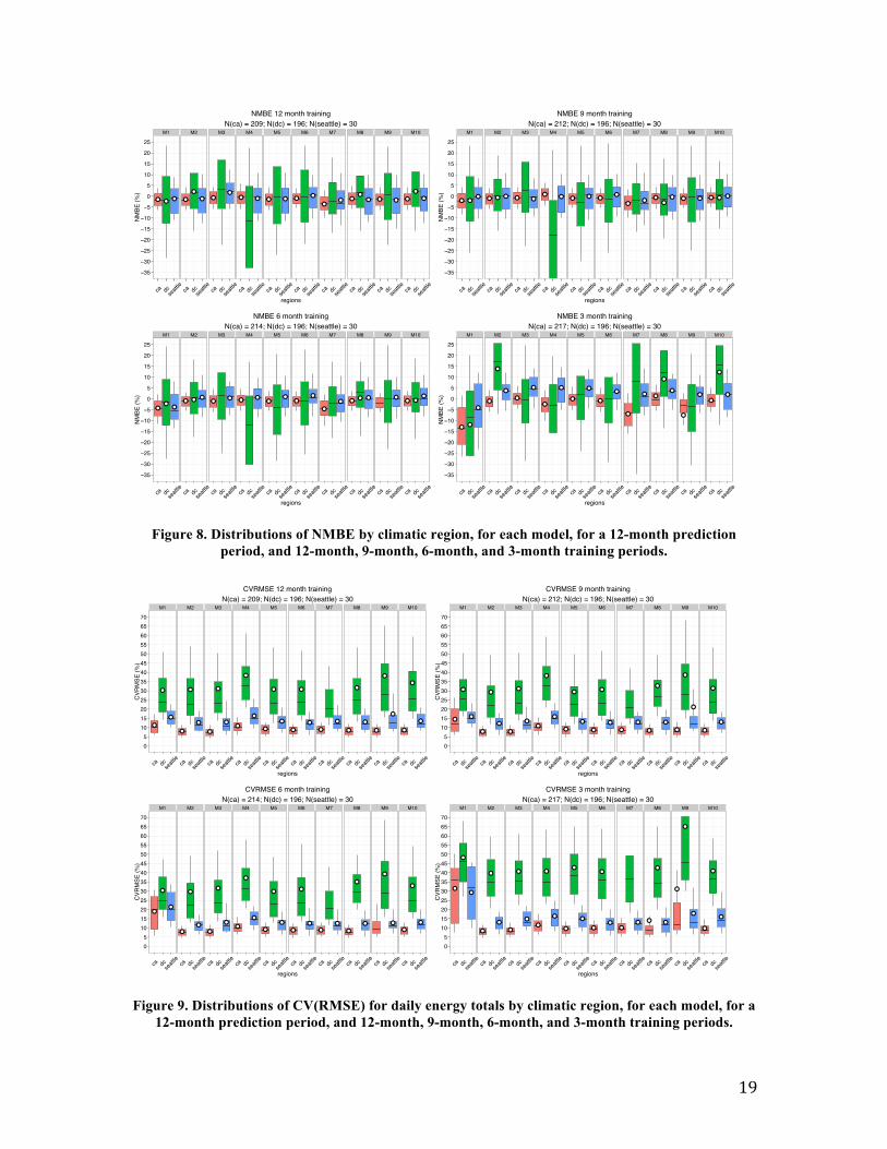
3.4 Results by Climate Zone Figures 8 and 9 shows the results of NMBE and CV(RMSE) for daily energy totals for regions independently, to supplement the aggregated findings that were detailed in Sections 3.1 through 3.3. In each plot, distributions of errors across the California dataset are shown in pink and plotted first, those for the Washington, DC dataset are shown in green and plotted second, and those for the Seattle dataset are shown in blue and plotted last. The number of buildings for which model predictions were generated is shown in the plot title, and the model IDs are displayed in grey across the top of each plot. These plots indicate that the median and the distribution of errors for the California data set (n=209) were modestly smaller than those for the Northwest (n=30), and those for Washington DC (n=198) were notably larger than both California and the Northwest.

●

●

●

●

●

●

●

●

●

●

−4.5

−4.0

−3.5

−3.0

−2.5

−2.0

−1.5

−1.0

−0.5

0.0

0.5

1.0

1.5

10 15 20 25CVRMSE (%)

NM

BE (%

)Model●

●

●

●

●

●

●

●

●

●

M1

M2

M3

M4

M5

M6

M7

M8

M9

M10

Median NMBE vs. Median CVRMSE for 12 month training

●

●

●

●●

●

●

●●

●

−4.5

−4.0

−3.5

−3.0

−2.5

−2.0

−1.5

−1.0

−0.5

0.0

0.5

1.0

1.5

10 15 20 25CVRMSE (%)

NM

BE (%

)

Model●

●

●

●

●

●

●

●

●

●

M1

M2

M3

M4

M5

M6

M7

M8

M9

M10


●

●●

●

●

●

●

●

●

●

−4.5

−4.0

−3.5

−3.0

−2.5

−2.0

−1.5

−1.0

−0.5

0.0

0.5

1.0

1.5

10 15 20 25CVRMSE (%)

NM

BE (%

)

Model●

●

●

●

●

●

●

●

●

●

M1

M2

M3

M4

M5

M6

M7

M8

M9

M10


●

●

●

●

●

●

●

●

−4.5

−4.0

−3.5

−3.0

−2.5

−2.0

−1.5

−1.0

−0.5

0.0

0.5

1.0

1.5

10 15 20 25CVRMSE (%)

NM

BE (%

)

Model●

●

●

●

●

●

●

●

●

●

M1

M2

M3

M4

M5

M6

M7

M8

M9

M10


19

Figure 8. Distributions of NMBE by climatic region, for each model, for a 12-month prediction period, and 12-month, 9-month, 6-month, and 3-month training periods.

Figure 9. Distributions of CV(RMSE) for daily energy totals by climatic region, for each model, for a 12-month prediction period, and 12-month, 9-month, 6-month, and 3-month training periods.

M1 M2 M3 M4 M5 M6 M7 M8 M9 M10

● ●● ● ●

●●

●● ● ● ● ●

●

●● ● ●

●● ● ● ●

●

−35

−30

−25

−20

−15

−10

−5

0

5

10

15

20

25

ca dcseatt

leca dcse

attle

ca dcseatt

leca dcse

attle

ca dcseatt

leca dcse

attle

ca dcseatt

leca dcse

attle

ca dcseatt

leca dcse

attle

regions

NM

BE (%

)

NMBE 12 month trainingN(ca) = 209; N(dc) = 196; N(seattle) = 30

M1 M2 M3 M4 M5 M6 M7 M8 M9 M10

●●

● ● ●● ● ●● ● ● ● ●

●

●●

● ●●

● ● ● ●●

−35

−30

−25

−20

−15

−10

−5

0

5

10

15

20

25

ca dcseatt

leca dcse

attle

ca dcseatt

leca dcse

attle

ca dcseatt

leca dcse

attle

ca dcseatt

leca dcse

attle

ca dcseatt

leca dcse

attle

regions

NM

BE (%

)


M1 M2 M3 M4 M5 M6 M7 M8 M9 M10

● ●●

●●● ●

● ● ●●

●●

●

●

● ●●● ●

●●

●

−35

−30

−25

−20

−15

−10

−5

0

5

10

15

20

25

ca dcseatt

leca dcse

attle

ca dcseatt

leca dcse

attle

ca dcseatt

leca dcse

attle

ca dcseatt

leca dcse

attle

ca dcseatt

leca dcse

attle

regions

NM

BE (%

)


M1 M2 M3 M4 M5 M6 M7 M8 M9 M10

●

●

●

●

●

●

●

●

●

●

●

●

●

●

●

● ●●

●

●

●●

●

●

−35

−30

−25

−20

−15

−10

−5

0

5

10

15

20

25

ca dcseatt

leca dcse

attle

ca dcseatt

leca dcse

attle

ca dcseatt

leca dcse

attle

ca dcseatt

leca dcse

attle

ca dcseatt

leca dcse

attle

regions

NM

BE (%

)


M1 M2 M3 M4 M5 M6 M7 M8 M9 M10

●

●

●

●

●

●

●

●

●

●

●

●

●

●

●

●

●

●

●

●

●

●

●

●

●

●

●

●

●

05

10152025303540455055606570

ca dcseatt

leca dcse

attle

ca dcseatt

leca dcse

attle

ca dcseatt

leca dcse

attle

ca dcseatt

leca dcse

attle

ca dcseatt

leca dcse

attle

regions

CVR

MSE

(%)

CVRMSE 12 month trainingN(ca) = 209; N(dc) = 196; N(seattle) = 30

M1 M2 M3 M4 M5 M6 M7 M8 M9 M10

●●

●

●

●

●

●

●

●

●

●

●

●

●

●

●

●

●

●

●

●

●

●

●

●

●

●

●

●

05

10152025303540455055606570

ca dcseatt

leca dcse

attle

ca dcseatt

leca dcse

attle

ca dcseatt

leca dcse

attle

ca dcseatt

leca dcse

attle

ca dcseatt

leca dcse

attle

regions

CVR

MSE

(%)


M1 M2 M3 M4 M5 M6 M7 M8 M9 M10

●●

●

●●

●

●

●

●

●

●

●

●

●

●

●

●

●

●●

●

●

●

●

●

●

●

●

05

10152025303540455055606570

ca dcseatt

leca dcse

attle

ca dcseatt

leca dcse

attle

ca dcseatt

leca dcse

attle

ca dcseatt

leca dcse

attle

ca dcseatt

leca dcse

attle

regions

CVR

MSE

(%)


M1 M2 M3 M4 M5 M6 M7 M8 M9 M10

●●

●

●

●

●

●

●

●

●

●

●

●

●

●

●●

●

●● ● ●

●

●

●

●

●

●

●

05

10152025303540455055606570

ca dcseatt

leca dcse

attle

ca dcseatt

leca dcse

attle

ca dcseatt

leca dcse

attle

ca dcseatt

leca dcse

attle

ca dcseatt

leca dcse

attle

regions

CVR

MSE

(%)


20

4. DISCUSSION

4.1 Absolute Model Performance

Overall, the interval data models that were tested were able to predict whole-building energy use with a high degree of accuracy for a large portion of the 537 buildings in the test dataset. For the standard whole-building case of twelve months training followed by twelve months of prediction, and for all models there was a tendency of a bias toward over-predicting energy use (negative NMBE), which has potential implications for pay-for-performance incentive designs. Average CV(RMSE) for daily energy totals was less than 13 for half of the buildings, and less than 24 for three quarters of them (except for model 4, a very naïve, simple model). This is promising for the industry. ASHRAE Guideline 14 specifies that CV(RMSE) during the training period, should be less than 25% if 12 months of post-measure data are used, and no uncertainty analysis is to be conducted [ASHRAE 2014]. The analyses in this study computed CV(RMSE) during the prediction period, which is expected to be even higher than that in the training period. Therefore, while not directly comparable, it appears that the models in this study are likely to meet the ASHRAE requirements for a large fraction of buildings. Median CV(RMSE) for 15-minute and daily energy totals was less than 25% for every model tested when twelve months of training data were used. With even six months of training data, median CV(RMSE) for daily energy total was under 25% for all models tested. Moreover, with NMBE ranging from approximately -1 to 4 for one quarter of the buildings in the dataset, and approximately -1 to -5 for another quarter, the results provide confidence that these M&V approaches will be applicable for many instances of multi-measure programs. This is because multi-measure programs commonly target larger savings, on the order of ten percent or more (for example, median retro-commissioning savings are 16% (Mills 2011)); with errors of just a couple of percent, there is less risk that savings will be ‘lost in the noise’. In addition, the accuracies achieved in this study were for a fully automated case. In practice, errors can be further reduced with the oversight of an engineer to conduct non-routine adjustments where necessary. For example, occupancy is not commonly available measured data, and therefore not included in the dataset, or as explanatory variables in the models. Were the buildings to experience significant changes in occupancy, non-routine adjustments might be merited, and could improve the accuracy of the savings that are quantified. When the training period was shortened from twelve months to nine, and then to six, there was a gradual degradation in predictive accuracy. Not surprisingly, a three-month training period was not long in general enough to capture the range of temperatures necessary to reliably predict energy over a the full range of temperatures and loads that are seen in a twelve-month period. Given the desire to shorten total time requirements for M&V, the modest increases in error incurred in shortening the training period, in some cases, even to six or three months, may be worth reducing the total time necessary to acquire data for the baseline period.

4.2 Climatic Differences The test dataset that was compiled for this analysis comprised whole-building data that represented a dataset of convenience, as opposed to design. Ideally, the buildings would be uniformly distributed across all climate zones, however it was not possible to obtain that level of diversity for this study. The data that were acquired were skewed to buildings from California

21

(ASHRAE Climate Zone 3), and Washington, DC (ASHRAE Climate Zone 4), with much less representation from other climates. An analysis of predictive accuracy was conducted for regions independently, to supplement the aggregated findings that also presented. Regional differences in model performance were observed; the median and distribution of errors for the California data set (n=209) were modestly smaller than those for the Northwest (n=30), and those for Washington DC (n=198) were notably larger than both California and the Northwest. This may be due to more extreme seasonal variations in outside air temperature in the Mid-Atlantic region. As the California dataset was provided by a participating model developer, while the Northwest and Washington DC datasets were contributed by non-developers, there is also a possibility that the California buildings were less randomly selected from the general commercial stock.

4.3 Relative Model Performance For the most part, each of the ten models performed equally well, according to the two metrics of focus in this study. When plots of median NMBE vs. CV(RMSE) were compared for the standard case of twelve months training and twelve months prediction, Models 1, 4, and 7 emerge as modest outliers; the other models analyzed are relatively tightly clustered together. When non industry-standard shorter training periods (nine, six, and three months) were considered, Models 1, 4, 7, and 9 emerged with relatively higher errors than the other models. However it is important to emphasize that only the median performance was investigated, and in many cases, the magnitude of the difference in errors between models was quite small. In spite of these relative differences in model performance, it is worth reiterating that absolute performance for all models tested was strong, and provided compelling evidence for their application to whole-building measurement and verification. The results section also noted that for some models, the mean error was extremely large. The fact that some buildings are simply not predictable based purely on outside air temperature, date and time is not surprising; there are buildings that are not operated in a predictable manner, for which other drivers of energy use are at play, or for which non-routine adjustments may be appropriate. Interestingly, in some cases the buildings that were poorly predicted by one model, were not the same as the buildings that were predicted poorly by the other models. In addition, most models were unable to generate predictions for at least some of the buildings in the data set – failure rates ranged from roughly zero to ten percent depending on the training period and particular model in question. These aspects of performance are likely due to differences in the underlying form of the models, how they were coded to run automatically in batch mode, their treatment of outliers in the training data, and the different mathematical approaches that they each use.

5. CONCLUSIONS AND FUTURE WORK The results of this work show that interval data baseline models, and streamlining through automation hold great promise for scaling the adoption of whole-building measured savings calculations using Advanced Metering Infrastructure (AMI) data. These results can be used to build confidence in model robustness, and also to pre-vet M&V plans for specific projects, given project requirements for uncertainty in reported savings. While uncertainty is not commonly considered today, it could hold value for evaluating and reducing project and investment risk. For example, ASHRAE’s published methods for computing fractional savings uncertainty depend on depth of savings, length of the training and prediction periods, and model CV(RMSE). “Look-up”

22

tables can be used to explore the likelihood that a given model will produce savings estimations that meet uncertainty and confidence requirements, for a specific set of buildings and expected depth of savings. After an efficiency project is initiated, these methods can be used as the project progresses to track achieved savings relative to expected savings, and perhaps even be used to indicate when measures are not correctly implemented, or when non-routine changes have occurred in the building operations or loads. Future work will focus on four key areas: 1) demonstration of these automated approaches in partnership with utilities, using data from buildings that have participated in whole-building programs or pilots; 2) exploration of industry demand for the objective model testing methods as presented in this paper, and identification of appropriate bodies to which the procedures should be transferred; 3) continued engagement of the evaluator, program manager and implementer community to collectively more clearly define uncertainty and confidence requirements for reporting gross energy savings; 4) investigation of how these approaches that use measured pre-measure energy use data as the baseline from which savings are calculated, can compare with evaluation requirements to consider code baselines.

ACKNOWLEDGEMENT

This work was supported by the Assistant Secretary for Energy Efficiency and Renewable Energy, Building Technologies Program, of the U.S. Department of Energy under Contract No. DE-AC02-05CH11231. The authors would like to thank the members of the project Technical Advisory Group for their participation and feedback throughout the course of the work. The authors also acknowledge each of the developers who submitted baseline models for inclusion in this study. Those who chose to self-identify include Buildings Alive Pty. Ltd. Of Sydney Australia, Paul Raftery and Tyler Hoyt of UC Berkeley’s Center for the Built Environment, Gridium Inc., Lucid Design Group, and Performance Systems Development of New York, LLC. Throughout the project, Cody Taylor of the Building Technologies Office provided valuable support and guidance. Finally we would like to thank those who contributed to the test dataset. Without a sufficient volume and diversity of data, meaningful insights would not have been possible.

REFERENCES ASHRAE Guideline 14 (2014). ASHRAE Guideline 14-2014 for Measurement of Energy and Demand Savings, American Society of Heating, Refrigeration and Air Conditioning Engineers, Atlanta, GA. Baechler, M., Williamson, J., Gilbride, T., Cole, P., Hefty, M., Love, P.M. (2010). Building America Best Practice Series, Volume 7.1. High performance home technologies: Guide to determining climate regions by county. Prepared for by Pacific Northwest National Laboratory, and Oakridge National Laboratory, August 2010, Report Number PNNL-17211. Consortium for Energy Efficiency (CEE) (2012). Summary of commercial whole building performance programs: continuous energy improvement and energy management and information systems. Consortium for Energy Efficiency.

23

Efficiency Valuation Organization (EVO) (2012). International performance measurement and verification protocol: concepts and options for determining energy and water savings, 1, EVO 10000-1:2012. Granderson, J., Piette, M. A., Ghatikar, G. (2011a). Building energy information systems: user case studies. Energy Efficiency, 4(1), 17-30. Granderson, J., Piette, M.A., Rosenblum, B., Hu, L. et al. (2011b). Energy information handbook: Applications for energy-efficient building operations. Lawrence Berkeley National Laboratory, Report Number LBNL-5272E. Granderson, J., Piette, M. A., Ghatikar, G., Price, P.N. (2009). Building energy information systems: state of the technology and user case studies. Lawrence Berkeley National Laboratory, Report Number LBNL-2899E. Granderson, J., Addy,N., Price,P., Sohn, M., (2015). Automated measurement and verification : Performance of public domain whole-building electric baseline models. Applied Energy, 144, 106-113. Granderson, J., Price, P.N. (2014). Development and application of a statistical methodology to evaluate the predictive accuracy of building energy baseline models. Energy, 66, 981-990. Haberl, J. S., Thamilseran, S. (1998). The great energy predictor shootout II: measuring retrofit savings. ASHRAE Journal, 40(1), 49-56. Jayaweera, T, Haeri, H, Kurnik, C. (2013). The Uniform Methods Project: Methods for Determining Energy Efficiency Savings for Specific Measures. National Renewable Energy Laboratory, April 2013. NREL Report # NREL/SR-7A30-53827. Mills, E. 2011. "Building Commissioning: A Golden Opportunity for Reducing Energy Costs and Greenhouse Gas Emissions in the United States." Energy Efficiency, 4(2):145-173 Kramer, H., Russell, J., Crowe, E., Effinger, J. (2013). Inventory of Commercial Energy Management and Information Systems (EMIS) for M&V Applications, prepared by PECI for Northwest Energy Efficiency Alliance, Report Number E13-264. Kreider, J. F., & Haberl, J. S. (1994). Predicting hourly building energy usage. ASHRAE Journal, 36(6), 1104-18. Mathieu, J.L., Price, P.N., Kiliccote, S., Piette, M.A. (2011). Quantifying changes in building electricity use, with application to Demand Response. IEEE Transactions on Smart Grid 2:507-518, 2011. Piette, M.A., Brown R.E., Price P.N., Page, J., Granderson, J., Riess, D., et al. (2013). Automated measurement and signaling systems for the transactional network. Lawrence Berkeley National Laboratory, December 2013. LBNL-6611E.

24

Price, P., Jump, D., Sohn, M., (2013). Functional Testing Protocols for Commercial Building Efficiency Baseline Modeling Software. Prepared by LBNL and QuEST for Pacific Gas and Electric. Report number LBNL-6593E, Pacific Gas and Electric Report Number ET12PGE5312.

25

APPENDIX

Statistical Goodness-of-Fit Metrics Goodness-of-fit metrics are commonly referred to with a diversity of names, and may be defined with subtle variations depending on their application. For clarity, the metrics that were considered for use in this study are defined in the following, with some discussion of their use specifically in the context of measurement and verification. Symbols that are used in the equations are as follows:

• N is the number of individual measurement points in an evaluation period • 𝑦! is the energy measured at the ith time interval • 𝑦! is the energy predicted at the ith time interval • 𝑦 is the mean energy use over the evaluation period

Total Bias (TB) This metric measures the total difference between the measured and model-predicted energy over a pre-determined evaluation period (e.g., three, six, or twelve months).

𝑇𝐵 = 𝑦! − 𝑦!

!

!

This metric is called “bias” rather than “error” because error is sometimes used to refer to the absolute difference between model predictions and measurements, ignoring the sign of the difference, whereas bias is specific to maintaining the sign of the difference. In general, bias is preferred when estimates of over- and/or under-prediction, or net differences, are noteworthy. For example, the metric could help ascertain whether an M&V payback program might in general over- or under-compensate for retrofit energy savings. Some reference documents define total bias as the observations minus the model predictions, and other documents define it as model predictions minus observations. Neither are incorrect, but their random use can be quite confusing since one cannot easily know, without looking at the equation, whether a positive bias means the model is over or under predicting the metered data. The tendency in ASHRAE Guideline 14-2014 is to subtract the model predictions from the data, and that convention is retained in this work. Hence, a positive bias means the model predicts lower energy use than was observed, and the magnitude of the difference is the energy (kWh) between the total energy predicted and measured (kWh). Total Error (TE) Total Error is similar to Total Bias, however it considers the absolute difference between model predictions and measurements over the evaluation period, ignoring the sign of the difference. This metric helps ascertain the overall performance of the model since both over- and under-prediction by the model are compiled. For the purposes of an M&V program, this metric is best considered as a compliment to a metric of bias.

𝑇𝐸 = 𝑦! − 𝑦!

!

!

26

Mean Bias (MB) Mean Bias is the total bias divided by the number of measurement points in the evaluation period. For example, an evaluation period of three months may have weekly, daily, or 15-minute measurements. The mean bias provides the expected under- or over-prediction of the model. This metric might be useful in applications when one desires to review how a model performs, in general, for any one-measurement comparison. However, this is usually not the scenario for most M&V applications, for a single building or across a portfolio of buildings.

𝑀𝐵 =1𝑁

(𝑦! − 𝑦!)!

!

Mean Absolute Percent Error (MAPE) This metric is the total normalized bias averaged over each of the energy measurements, or subtotaled over fixed time intervals, for the evaluation period. The metric provides an overall assessment of the general percent error in model-predicted energy use, as one proceeds through the evaluation period.

𝑀𝐴𝑃𝐸 = 1𝑁

𝑦! − 𝑦!𝑦!

×100!

!

Because the metric is normalized by the meter reading, it provides an equitable measure of model performance for predicting both high and low energy. This metric is popular for providing a general assessment of model performance since it normalizes the size of errors that are due to larger versus smaller building loads, and can be averaged over each measurement or fixed time interval. This metric is also referred to as mean normalized error. Normalized Mean Bias Error (NMBE) This metric is effectively a total percent error over the evaluation period, e.g., -5% error would indicate that the model over predicted the actual metered energy use by 5%. In this context, the use of percent differences rather than absolute differences normalizes the size of errors that are due to larger versus smaller building loads. Similarly, the directionality of the error reveals under- versus over-predictions, which has an implication on over- versus under-payment, when pay-for-performance is a consideration. Variations of this metric are also referred to as percent total bias, absolute percent bias error, or net determination bias.

𝑁𝑀𝐵𝐸 = 1𝑁 (𝑦! − 𝑦!)!

!

𝑦×100

Root Mean Squared Error (RMSE) This is a popular metric that measures the average squared difference between predictions and data over the evaluation period. This metric is preferred over mean bias when one desires to assess large differences between model predictions and measurements (owing to the squaring of the differences) and when total energy is more relevant than relative energy (owing to no normalization).

27

𝑅𝑀𝑆𝐸 = 1𝑁

𝑦! − 𝑦! !!

!

Large differences at even one of the time intervals will result in disproportionately high values of root mean squared error. In the context of comparing M&V models the use of this metric will thus tend to highlight those models that follow the general temporal trend in the measured energy. Models with low RMSE will tend to predict high energy use when metered energy use is high, and the model will predict low energy use when the metered energy use is low. Coefficient of Variation of the Root Mean Squared Error (CV(RMSE)) This is the RMSE normalized by the mean energy use over the evaluation period. This measure is particularly helpful when reviewing model-to-data comparisons of several buildings simultaneously, because it regulates the relative performance in buildings that use high amounts of energy against those that use low amounts of energy. The equation is similar to a coefficient of variation (which is the standard deviation divided by the mean) in that it provides the difference between predictions and data relative to the mean overall energy.

𝐶𝑉 𝑅𝑀𝑆𝐸 =

1𝑁 𝑦! − 𝑦! !!

!

𝑦×100

Coefficient of Determination (R2 or R Squared) This metric measures how well interval energy data agree with a linear relationship to model predictions, at the same time intervals over the evaluation period. There is often some confusion on whether model predictions are compared the actual data, or vice versa, whether the actual data are compared to the model predictions. The choice results in a different value of R Squared. In the M&V application, both options are possible, so the convention should be explicitly stated when reporting values of the metric.

𝑅! = 1 −𝑦! − 𝑦! !!

!

𝑦! − 𝑦 !!!

28

Description of Models Tested For cases in which the model developer consented, more detailed descriptions of the baseline models are provided below. M4: Mean Week In this model the predictions of the future values, for a given day of the week d and time t, are equal to the average of the training data for this particular day and time, then we can write the predictions as

𝑦 𝑑, 𝑡 =1

𝑁(𝑑, 𝑡)𝑦(𝑑! , 𝑡!)

!(!,!)

!!!

where 𝑦(𝑑! , 𝑡!) is the value of the ith week of the training data, and 𝑁(𝑑, 𝑡) is the number of weeks in the training data, which have values for the day of the week d and time t. M5: Time of Week and Temperature In the Time of Week and Temperature model, the predicted load is a sum of two terms: (1) a “time of week effect” that allows each time of the week to have a different predicted load from the others, and (2) a piecewise-continuous effect of temperature. The temperature effect is estimated separately for periods of the day with high and low load, to capture different temperature slopes for occupied and unoccupied building modes. The model is described in detail in Mathieu et al. (2011), and the method is described in detail in Granderson et al. (2013).

For each day of the week, the 10th and 90th percentile of the load were calculated; call these L10 and L90. The first time of that day at which the load usually exceeds the L10 + 0.1*(L90-L10) is defined as the start of the “occupied” period for that day of the week, and the first time at which it usually falls below that level later in the day is defined as the end of the “occupied” period for that day of the week.

M6: Weighted Time of Week and Temperature

This model is the Time-of-Week and-Temperature model with the addition of a weighting factor to give more statistical weight to days that are nearby to the day being predicted. This is achieved by fitting the regression model using weights that fall off as a function of time in both directions from a central day. In the implementation used in this work, the weight parameter is set to fourteen, placing more weight on the most recent two weeks of data.

M7. Ensemble approach combining nearest neighbors and a generalized linear model, developed by Lucid Design Group.

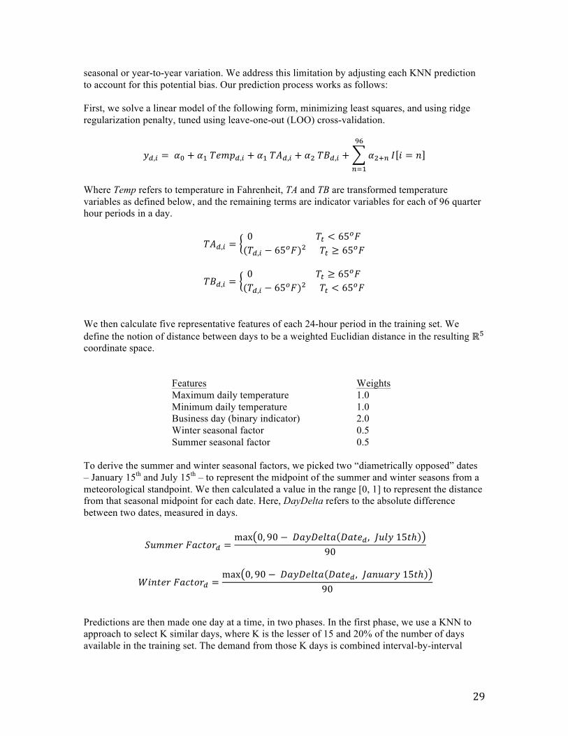
Lucid’s model employed a sequential ensemble approach, first generating predictions using K-nearest-neighbors (KNN), and then adjusting the KNN output with help of a ridge regression model. The intuition underlying this approach is that KNN is generally strong in capturing nonlinearities in the relationship between prediction and outcome variables, especially for low-dimensional problems. However, its applicability is bounded by the availability of sufficiently “nearby” neighbors for each prediction made. In an M&V context, this problem might manifest as negative bias when predicting demand on hot days, especially if the training set spans a period of mostly cooler temperatures, because of either

29

seasonal or year-to-year variation. We address this limitation by adjusting each KNN prediction to account for this potential bias. Our prediction process works as follows: First, we solve a linear model of the following form, minimizing least squares, and using ridge regularization penalty, tuned using leave-one-out (LOO) cross-validation.

𝑦!,! = 𝛼! + 𝛼! 𝑇𝑒𝑚𝑝!,! + 𝛼! 𝑇𝐴!,! + 𝛼! 𝑇𝐵!,! + 𝛼!!!

!"

!!!

𝐼 𝑖 = 𝑛

Where Temp refers to temperature in Fahrenheit, TA and TB are transformed temperature variables as defined below, and the remaining terms are indicator variables for each of 96 quarter hour periods in a day.

𝑇𝐴!,! =0 𝑇! < 65!𝐹(𝑇!,! − 65!𝐹)! 𝑇! ≥ 65!𝐹

𝑇𝐵!,! =0 𝑇! ≥ 65!𝐹(𝑇!,! − 65!𝐹)! 𝑇! < 65!𝐹

We then calculate five representative features of each 24-hour period in the training set. We define the notion of distance between days to be a weighted Euclidian distance in the resulting ℝ! coordinate space.

Features Weights Maximum daily temperature 1.0 Minimum daily temperature 1.0 Business day (binary indicator) 2.0 Winter seasonal factor 0.5 Summer seasonal factor 0.5

To derive the summer and winter seasonal factors, we picked two “diametrically opposed” dates – January 15th and July 15th – to represent the midpoint of the summer and winter seasons from a meteorological standpoint. We then calculated a value in the range [0, 1] to represent the distance from that seasonal midpoint for each date. Here, DayDelta refers to the absolute difference between two dates, measured in days.

𝑆𝑢𝑚𝑚𝑒𝑟 𝐹𝑎𝑐𝑡𝑜𝑟! =max 0, 90 − 𝐷𝑎𝑦𝐷𝑒𝑙𝑡𝑎 𝐷𝑎𝑡𝑒! , 𝐽𝑢𝑙𝑦 15𝑡ℎ

90

𝑊𝑖𝑛𝑡𝑒𝑟 𝐹𝑎𝑐𝑡𝑜𝑟! =max 0, 90 − 𝐷𝑎𝑦𝐷𝑒𝑙𝑡𝑎 𝐷𝑎𝑡𝑒! , 𝐽𝑎𝑛𝑢𝑎𝑟𝑦 15𝑡ℎ

90

Predictions are then made one day at a time, in two phases. In the first phase, we use a KNN to approach to select K similar days, where K is the lesser of 15 and 20% of the number of days available in the training set. The demand from those K days is combined interval-by-interval

30

using a weighted average, where the weight for each day decreases with increasing distance from the day being predicted.

𝑤𝑒𝑖𝑔ℎ𝑡! ∝1

1 + 𝐷𝑖𝑠𝑡𝑎𝑛𝑐𝑒(𝐷𝑎𝑡𝑒!"#$%&'%(), 𝐷𝑎𝑡𝑒!)

The output of this step is 96 values 𝑞!,! predicting demand each quarter hour interval i of the day d being predicted. The second and final step is to adjust that result using our linear model from the first step. To do that, we use our linear model to predict demand 𝑟!,! for each interval i of each day d and in our set of nearest neighbors. We also use the same linear model to predict demand for the day being predicted. Finally, we take the interval-by-interval difference between the nearest neighbor predictions and the target day prediction, and adjust the KNN output by those differences to generate a final prediction:

𝑦!,! = 𝑞!,! − 0.6 × 𝑤𝑒𝑖𝑔ℎ𝑡! 𝑟!,! − 𝑟!"#$%&'%(),!

!

!!!

We inserted the 0.6 factor because we found that applying the full adjustment overcompensated for the local biases of KNN alone, and reduced the RMSE in cross validation trials. Future improvements on this approach might attempt to tune that value as a parameter rather than use a “magic number.”

Assessment of Automated Measurement and … of Automated Measurement and Verification (M&V) Methods...

Documents

Transcript of Assessment of Automated Measurement and … of Automated Measurement and Verification (M&V) Methods...