Assessment of an Unstructured-Grid Method for Predicting Aerodynamic Performance of Jet Flaps

*Josue Cruz and Scott G. Anders*

NASA Langley Research Center, Hampton, VA, 23681

The application of a Computational Fluid Dynamics tool to a jet flap control effector on an elliptical airfoil-section wing was investigated. The study utilized the Tetrahedral Unstructured Software System developed at NASA Langley Research Center. The Reynolds-averaged Navier-Stokes flow solver code used was USM3D. The CFD-based jet flap simulations were compared to experimental results from a wind tunnel test conducted at the NASA Langley Transonic Dynamics Tunnel. The wind tunnel model consisted of a six percent thick elliptical airfoil with a modified trailing edge. The jet flap was located at 95% chord and exited at 90 degrees to the lower surface. The experimental model was designed to promote two-dimensional flow across the wing. It was found that the CFD simulation had to model the three-dimensional geometry of the experiment in order to obtain good agreement. Tests were performed at two Mach numbers at several different jet momentum coefficients. In order to be consistent with the experimental method, the CFD lift and pitching moment values were determined by integrating the pressures over the wing.

Nomenclature c = chord, inches CFD = computational fluid dynamics C = total lift from USM3D L C = sectional lift coefficient l

pressurelC = pressure contribution to lift coefficient

thrustlC = thrust contribution to lift coefficient C = quarter chord pitching moment m

pressuremC = pressure contribution to pitching moment coefficient

thrustmC = thrust contribution to pitching moment coefficient

pC = pressure coefficient

lpC = lower surface pressures coefficients

upC = upper surface pressures coefficients C = momentum coefficient μEXP = experiment

g = gravitational constant, ⎟⎟⎠

⎞⎜⎜⎝

⎛

−−

2174.32slbfftlbm c

M = Mach number m& = mass flow rate, lbm/s N = number of cells

2inlbf

∞P = freestream static pressure,

plenumoP = total pressure (plenum), 2inlbf

* Aerospace Engineer, Advanced Aerospace System Branch, Hampton, VA/411

American Institute of Aeronautics and Astronautics

1

2inlbf

∞q = freestream dynamic pressure,

R = gas constant, ⎟⎠⎞

⎜⎝⎛

°−−

Rlbmlbfft34.53

r = residual S = model surface area, inches2

TDT = Transonic Dynamics Tunnel To = total temperature (plenum) (°R)

sftU = ideal jet velocity (assumes isentropic expansion to freestream pressure), jet

x = chordwise distance from leading edge, inches xjet = jet chordwise distance from leading edge, inches x/c = non dimensional chordwise distance y/b = non dimensional span location α = angle of attack, degrees ΔCl = change in lift coefficient from Cµ=0.0 case ΔC = change in pitching moment coefficient from Cm µ=0.0 case γ = ratio of specific heats

I. Introduction HE application of a Computational Fluid Dynamics (CFD) tool to a jet flap control effector on an elliptical airfoil-section wing has been investigated. The objective was to predict jet flap characteristics up to transonic

speeds and to compare the results to experimental data. The Tetrahedral Unstructured Software System (TetrUSS) developed at NASA Langley Research Center was used in this investigation.

T The jet flap concept has been experimentally investigated since the 1930’s. A jet flap acts as a pneumatic flap and behaves similar to a mechanical flap by producing an increase in circulation and therefore an increase in lift. Davidson(1) describes that “the gas stream from a jet flap acts like a larger Fowler flap”. Yoshihara and Zonars describe the jet flap as reminiscent of a mechanical flap and include characteristics such as an increase of the upper surface suction plateau, near-uniform increase of the lower surface overpressures, and a rearward displacement of the terminating shock wave, where all effects add to the lift(2). Spence(3) states that the jet flap “supplies lift both by the reaction to the vertical momentum of the jet, which appears as pressure on the internal ducting, and by the vertical components of the pressures on the outer surface of the airfoil”. The CFD-based jet flap simulations were compared to experimental results from a wind-tunnel test that was conducted in NASA Langley Research Center’s Transonic Dynamics Tunnel. The jet flap was created by exhausting a stream of high pressure air from a lower surface slot that was close to the trailing edge (Fig. 1a). The jet sheet exited at 90° degrees to the surface (Fig. 1b). a) b)

Leading Edge Trailing Edge Plenum

Computational Inflow BoundaryFlow Aperture

Figure 1. a) Cross Section, b) Trailing Edge Schematic and Plenum.

American Institute of Aeronautics and Astronautics

2

II. Wind Tunnel Experiment

A. Experiment Set-up The experimental model consisted of a modified six percent thick elliptical two-dimensional airfoil with 0.75%

circular-arc camber and zero leading and trailing edge sweep. The model included a circular end plate of 30 in. diameter to promote two-dimensional flow across the wing and a splitter plate that offset the model 40 in. from the tunnel wall (Fig. 2). In addition, the model had two separate and isolated plenums for circulation control (Fig. 1a). Both plenums were used for circulation control testing as reported in reference 4. Only the lower plenum was used for the jet flap study.

The wing was instrumented with a total of 157 static and total pressures taps of which 93 (47 upper & 46 lower) surface pressure taps were located at y/b=0.5. The sectional lift and moment coefficients were calculated by integrating the pressure measurements at this location. The model did not include a balance. Both the experiment and the computation focused on two conditions. The subsonic condition was at a Mach number of 0.3 at an angle of attack of 6 degrees at a Reynolds number of 400,000/ft. The transonic condition was at a Mach number of 0.8

at an angle of attack of 3 degrees at a Reynolds number of 900,000/ft. The momentum coefficients, Cµ, for the jet flap data ranged from 0.006 to 0.042. Additional information on the experimental instrumentation can be found in reference 4.

Figure 2. Experimental Model.

B. Calculation of Aerodynamic Coefficients The experimental airfoil used pressure and temperature measurements as the primary instrumentation. The

sectional lift and quarter-chord pitching moment coefficients were calculated from these measurements since the model did not have a balance installed in it. In order to provide a more direct comparison to the experimental results, the aerodynamic coefficients found from the CFD solutions were calculated with the same method. The sectional coefficients included a pressure term and a thrust term but did not include a skin friction term since the experiment did not account for this. Equations 1 through 6 show how the sectional coefficients were calculated for both the experiment and the CFD solutions.

thrustpressure lll CCC +=

(1)

( ) )cos(1

0

α∫ ⎟⎠⎞

⎜⎝⎛−=

cxdCCC ulpressure ppl

(2)

)cos(αμCC thrustl =

(3)

thrustpressure mmm CCC +=

(4)

( )∫ ⎟⎠⎞

⎜⎝⎛

⎟⎟⎠

⎞⎜⎜⎝

⎛⎟⎠⎞

⎜⎝⎛−−=

1

0

25.0cxd

cxCCC ulpressure ppm

(5)

American Institute of Aeronautics and Astronautics

3

⎟⎟⎠

⎞⎜⎜⎝

⎛−= 25.0

cx

CC Jetthrustm μ

(6)

The experimentally determined momentum coefficient was calculated using plenum pressure and temperature measurements and the measured mass flow rate from a Venturi meter. The momentum coefficient found from the CFD solutions was calculated similarly. The momentum coefficient is defined in equation 7. The ideal jet velocity used in equation 8 was calculated(5) based on the assumption that the jet flow expands isentropically from the plenum pressure to the free stream static pressure. This is the common and historically accepted method for calculating the jet velocity.

SqUm

C jet

∞

=&

μ

(7)

⎥⎥⎥

⎦

⎤

⎢⎢⎢

⎣

⎡

⎟⎟⎠

⎞⎜⎜⎝

⎛−⎟⎟

⎠

⎞⎜⎜⎝

⎛−

=

−

∞γγ

γγ

1

11

2Plenumo

cojet PPgRTU

(8)

III. Computational Methods TetrUSS is a software system consisting of four modules. It is a loosely integrated unstructured-grid based CFD

system that provides ready access to rapid higher-order analysis and design capability for the applied aerodynamicist6). TetrUSS uses Gridtool(7,8) (8) for geometry setup, VGRID for grid generation, USM3D(8) for the flow solver, and VGPLOT(8) for postprocessing. The Reynolds averaged Navier-Stokes code, USM3D, was used for the calculations presented in this paper. The code uses a cell centered, upwind biased, finite volume and implicit/explicit algorithm to solve the compressible Euler and Navier-Stokes equations on an unstructured tetrahedral mesh(9-11). All the results obtained for this CFD simulation were performed using the Spalart-Allmaras(12) turbulence model. Although this was the only turbulence model available, newer versions of USM3D will include several two-equation turbulence models.

All the computations were performed using the NASA Ames Columbia supercomputer system. Typically, from 7 to 28 wall clock hours were needed for each run, depending on size of the grid, with 96 processors working as a parallel system. The required CPU hours ranged from 660 to 2700 hours of processor time. Convergence was based on lift, pitching moment, and drag histories as well as the residual convergence.

Splitter Plate

End plate IV. Grid Study Generating the grid was difficult because of the complexity of the

geometry (Fig. 3). The aperture and surrounding region were the biggest problem areas for the grid generation, since it was necessary to substantially refine the grid size which consequently in some cases did not interpolated well with the rest of the grid. The problem was not so much the grid refinement but how to accomplish the growth of the grid in this area. The aperture area and corresponding grid are shown in figures 4 and 5. There were five different grid densities generated. These five grid densities were used to perform a sensitivity study in order to find the asymptotic region. The results are shown in figures 6 and 7 where C represents the sectional lift coefficient and the

Figure 3. Grid Model. l

American Institute of Aeronautics and Astronautics

4

32−

Nhorizontal axis term, , assumes a second order accuracy of the solution on a three-dimensional grid. The selected grid used for this study contained 20.6 million cells and is indicated in the asymptotic region of figures 6

and 7 at 32−

N 32−

N= 0.133. The most dense grid (26.6 million cells) in this graph is at a =0.112 (Fig. 6, 7) whereas

the coarsest grid (15.6 million cells) is at 32−

N =0.160 (Fig. 6, 7). The residual convergence for the selected grid is typical for a complex geometry using USM3D and is shown in figure 8. The peak in figure 8 at 1000 iterations is due to the change from a first to a second order gradient computed analytically based on Taylor series. As an example, the convergence of the total lift coefficient ,which was computed by USM3D, is presented in figure 9. LC

Figure 4. Cross Section of the 3D Model and Grid at Figure 5. Aperture Cross Section the Trailing Edge. Close-Up.

0.75

0.76

0.77

0.78

0.79

0.80

0.10 0.12 0.14 0.16 0.180.64

0.65

0.66

0.67

0.68

0.69

0.70

0.10 0.12 0.14 0.16 0.18

Selected Grid Selected Grid

CC l l

32−

N 32−

N

Figure 6. Grid Sensitivity Study at Figure 7. Grid Sensitivity Study at Mach=0.30, Alpha=6.00°, C Mach=0.80, Alpha=3.00°, Cμ=0.012. μ=0.0074.

American Institute of Aeronautics and Astronautics

5

0.00.10.20.30.40.50.60.70.80.9

0 1000 2000 3000 4000 5000 6000-4.5-4.0-3.5-3.0-2.5-2.0-1.5-1.0-0.50.00.5

0 1000 2000 3000 4000 5000 6000

Residual CL

⎟⎟⎠

⎞⎜⎜⎝

⎛

orrLog

There were three different CFD domain geometries evaluated for the jet flap model. The first domain consisted

of using a symmetry plane at mid-span (y=30in) (Fig. 10a). The CFD domain for this geometry was 5x22x22 chords. The main purpose of using the symmetry plane was to reduce the number of grid points but the results were disappointing as discussed in the results section. The second domain consisted of the full configuration (Fig. 3) with the splitter plate. The CFD domain for this configuration was 10x22x22 chords (Fig. 10b, 10c). The outer boundaries of the CFD domain used an inflow/outflow boundary condition as defined in USM3D(8). The plenum inflow (Fig. 1b) boundary condition(8) is used to introduce the jet mass flow. The boundary condition was defined by setting the CFD Po and To equal to the experimentally measured Po and To. This method was preferred because Po and To were trusted experimental values and could be directly entered into the CFD input file. This method can result in slight differences in Cµ values due to small geometry differences between the CFD and experiment. The 10x22x22 chord domain was used for the entire analysis. A third domain was used to perform a verification test to check the sensitivity of the solution to the proximity of the outer boundaries. This was performed with a CFD domain that was 10x66x66 chords. Results showed a difference in the sectional lift of less than 0.96 %.

Figure 8. Typical USM3D Residual Convergence at

Mach=0.80, Alpha=3.00°, Cμ=0.0074.

Iterations Iterations

Figure 9. Lift Convergence at Mach=0.80 Alpha=3.00°, Cμ=0.0074.

5 ChordsWide

22 ChordsHeight

10 Chords Wide

Symmetry Plane

a) b) c)

End Plate

Splitter Plate

End Plate

AirfoilAirfoil

Figure 10. View from Downstream of CFD Domains a) 5x22x22 Chords Domain, b) 10x22x22 Chords Domain, c) Grid Domain.

American Institute of Aeronautics and Astronautics

6

V. Results

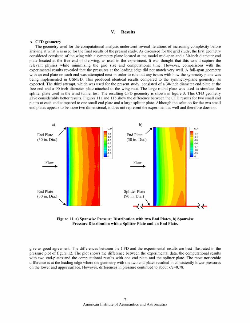
A. CFD geometry The geometry used for the computational analysis underwent several iterations of increasing complexity before arriving at what was used for the final results of the present study. As discussed for the grid study, the first geometry considered consisted of the wing with a symmetry plane located at the model mid-span and a 30-inch diameter end plate located at the free end of the wing, as used in the experiment. It was thought that this would capture the relevant physics while minimizing the grid size and computational time. However, comparisons with the experimental results revealed that the pressures at the leading edge did not match very well. A full-span geometry with an end plate on each end was attempted next in order to rule out any issues with how the symmetry plane was being implemented in USM3D. This produced identical results compared to the symmetry-plane geometry, as expected. The third attempt, which was used for the present study, consisted of a 30-inch diameter end plate at the free end and a 90-inch diameter plate attached to the wing root. The large round plate was used to simulate the splitter plate used in the wind tunnel test. The resulting CFD geometry is shown in figure 3. This CFD geometry gave considerably better results. Figures 11a and 11b show the difference between the CFD results for two small end plates at each end compared to one small end plate and a large splitter plate. Although the solution for the two small end plates appears to be more two dimensional, it does not represent the experiment as well and therefore does not

a) b)

End Plate End Plate (30 in. Dia.) (30 in. Dia.)

Flow Flow

End Plate Splitter Plate (30 in. Dia.) (90 in. Dia.)

Figure 11. a) Spanwise Pressure Distribution with two End Plates, b) Spanwise Pressure Distribution with a Splitter Plate and an End Plate.

give as good agreement. The differences between the CFD and the experimental results are best illustrated in the pressure plot of figure 12. The plot shows the difference between the experimental data, the computational results with two end-plates and the computational results with one end plate and the splitter plate. The most noticeable difference is at the leading edge where the geometry with the two end plates resulted in consistently lower pressures on the lower and upper surface. However, differences in pressure continued to about x/c=0.78.

American Institute of Aeronautics and Astronautics

7

-3.4

-3.0

-2.6

-2.2

-1.8

-1.4

-1.0

-0.6

-0.2

0.2

0.6

1.0

0.0 0.2 0.4 0.6 0.8 1.0

EXP with one End Plate and the Splitter Plate

CFD with one End Plate and the Splitter Plate CFD with two End Plates

x/c

Cp

Figure 12. Pressure Distribution at Mach=0.3, Alpha=6.0°, Cμ=0.012. The diameter of the large splitter plate (90 inches) was somewhat arbitrarily chosen to be three times the smaller end plate. In comparison, the rectangular splitter plate used in the wind tunnel experiment was 120 inches high (perpendicular to freestream flow) and 144 inches long (in the direction of the freestream flow). A circular end plate was used in the CFD simulation because it simplified the geometry and thus the grid. It also simplified the flowfield by avoiding the ninety-degree corners on the actual splitter plate. After the CFD analysis for this study was completed it was decided to check the effect of modeling the actual splitter plate. The CFD splitter plate was 75% as high and had 37% of the area of the experimental splitter plate. Three cases were run. Two cases were run where the momentum coefficient was zero, one at Mach=0.3 and one at Mach=0.8. The third case used the highest momentum coefficient simulated in the CFD for the transonic analysis (Mach = 0.8). For the Cµ=0 cases there was a 2% increase in lift at Mach=0.3 and a 3% increase at Mach=0.8. For the high momentum coefficient case at Mach=0.8 there was a 1% decrease in lift compared to the circular splitter plate. There was also slightly better agreement with shock location compared to the experimental data. The small differences between the results from the rectangular splitter plate and the results from the 90-inch diameter splitter plate did not warrant rerunning the study. The key point found from the geometric iterations was that although the use of the smaller end plate and symmetry plane provided a good approximation of two-dimensional flow over the wing (Fig. 11a), it did not appropriately model the flow experienced in the wind tunnel experiment. The full configuration with the end plate and the splitter plate (Fig. 3, 10b) was required to get good agreement, which will be discussed in more detail.

B. CFD Simulation As mentioned before, the jet flap behaves like a mechanical flap. The Mach number contour plots presented in

figures 13 and 14 for Mach=0.8 display this behavior by showing how the flowfield changes with momentum addition. These two figures illustrate the notion that the jet flap behaves like a mechanical flap; specifically, a gurney flap. It can be seen that the jet flap creates an area of lower Mach numbers upstream of it and deflects the streamlines downward just as a small physical flap would. The obvious advantage of the jet flap is that a mechanical system is not needed. However, one important disadvantage of the jet flap is that it has decreasing control authority as dynamic pressure increases whereas a mechanical flap would have increasing authority with higher dynamic pressure. In figures 15 and 16 it is apparent in the Mach 0.8 case shown that momentum influences the velocities over the entire wing. Some of this effect was also apparent in figure 14 where it can be seen that the flow reaches sonic conditions above the trailing edge upper surface. Also note the change in the shock location in figure 16. The no-blowing plot (fig. 15) has a shock location of approximately x/c = 0.3 whereas the momentum case has a shock location of approximately x/c = 0.5. The movement of the shock location towards the back of the wing is a direct consequence of jet momentum, just as a change in flap setting would cause. While there is no shock at lower Mach numbers, a similar global effect on the flowfield occurs at Mach=0.3.

American Institute of Aeronautics and Astronautics

8

Figure 13. Trailing Edge Flow Visualization Figure 14. Trailing Edge Flow Visualization at Mach=0.8, Alpha=3.0°, Cμ=0.0000.

At Mach=0.8, Alpha=3.0°, Cμ=0.0115.

Figure 16. Mach Contours at Mach=0.8 Figure 15. Mach Contours at Mach=0.8 Alpha=3.0°, CAlpha=3.0°, Cμ=0.0000. μ=0.0115.

As shown in figures 17 through 19, CFD results match reasonably well for the Mach 0.3 cases. Figure 17 shows the Cp profiles, which match well for the blowing and no-blowing cases. One can easily see how the momentum coefficient, C , influences the pressure over the entire wing. Note that the Cµµ values from the CFD simulation did not exactly match the values from the experiment. This is due to the way that boundary conditions were set, as explained earlier. The CFD simulation correctly predicts the pressure peak at the leading edge of the wing as it experiences an increase in suction pressure with increasing Cµ. The pressures are nearly uniformily shifted over the first 50% of chord. The trailing edge shows larger changes in pressure on both the upper and lower surfaces and this behavior is captured well by the CFD simulations. Figure 18 shows good correlation between the experiment and CFD for the change in sectional lift coefficient with increased Cµ. This was expected since it has already been shown that the Cp profiles match well. The CFD simulation was consistently low over the entire range of Cµ. The reason for this is unknown. The no-blowing Cl for the experiment was Cl=0.57 as compared to Cl=0.52 for the CFD simulation. Figure 19 shows the C characteristics. Pitching moment is a linear function of Cm l, as expected, and this trend is predicted well by the simulation. With higher Cl the experiment and the CFD produce more negative (nose down) pitching moment due to the higher suction pressures aft of the quarter chord(13).

Figures 20 through 22 show the results for the Mach 0.8 condition. The Cp profiles found from CFD match the experimental results well except that the shock location is predicted to be further forward (Fig. 20). One reason for this could be that the local Mach number in the immediate vicinity of the model could have been higher than the

American Institute of Aeronautics and Astronautics

9

reported tunnel Mach number which is what was used for the CFD freestream Mach number. This type of tunnel test section Mach number variation is possible if there was sufficient local acceleration due to the splitter plate and model. The effect of increased Mach number was investigated by performing a CFD simulation where the freestream Mach number was increased by 1%. This small change resulted in a match to the shock location found in the experiment (Fig. 23). It is plausible that a 1% increase in local Mach number could be caused by the blockage created by the combination of the splitter plate, its mounting hardware, and the model itself(14-15). Also shown in figure 20 is that aft of about 80% chord, there is an unexplained underprediction of the amount of suction on the upper surface. Figure 21 shows good correlation between the experiment and CFD for the change in sectional lift coefficient with increased Cµ for Mach=0.8. The agreement for the Mach=0.8 condition is better than what was seen for the Mach=0.3 condition (Fig. 18). The no-blowing Cl found in the experiment was Cl=0.47 as compared to Cl=0.43 for the CFD simulation. The pitching moment characteristics (Fig. 22) at transonic Mach number show increasingly negative pitching moment as Cµ, and thus Cl, increases. Although the same trend is shown by the theoretical and experimental methods, the CFD slightly underpredicts the magnitude of the pitching moment. This is not surprising since the CFD underpredicts the level of suction on the upper surface on the aft of the airfoil (Fig. 20). The negative pitching moment behavior with increasing lift, as stated by Grahame and Headley(13), is caused by “the higher pressures aft of the quarter chord, rearward shift of shock, and the separation which develops aft of the shock on the wing upper surface”. All of these things are apparent in the present data set.

VI. Summary and Conclusions The application of a Computational Fluid Dynamics tool to a jet flap control effector on an elliptical airfoil-

section wing was investigated. The study utilized the Tetrahedral Unstructured Software System developed at NASA Langley Research Center. The Reynolds-averaged Navier-Stokes flow solver code used was USM3D. The CFD-based jet flap simulations were compared to experimental results from a wind tunnel test conducted at the NASA Langley Transonic Dynamics Tunnel.

The CFD simulation matches the experimental Cp profile well and, as expected, this led to good agreement in the predicted lift augmentation and pitching moment characteristics. The use of a geometric model that closely matched the experimental set-up was critical in obtaining good agreement. It is important to emphasize that even though the experiment was designed to promote two-dimensional flow, a three-dimensional simulation was necessary to get good correlation between the experimental and simulation results. The results of this study show that the CFD tool utilized here could be used for future studies of jet flap applications. To the best of our knowledge, this is the first time TetrUSS has been used and validated for jet flap applications.

Acknowledgments The authors gratefully acknowledge the help and support from Neal T. Frink, Stuart K. Johnson, Richard F.

Catalano, Robert P. Weston, Thomas M. Moul and William J. Small. Although it was not presented, the authors would like to thank Lawrence Green for the verification and validation support he provided for this study. Details of the effort will be included in an upcoming publication.

American Institute of Aeronautics and Astronautics

10

References 1Davidson I. M., B.Sc. and A.F.R.Ae.S., “The Jet Flap,” Royal Institution, 960th Lecture, London, W.1, 10/20/1955, pp. 25-

60. 2Yoshihara H. and Zonars D., “The Transonic Jet Flap-A Review of Recent Results,” National Advisory Committee for

Aeronautics, Technical Note 3863, 1956. 3Spence D.A., “The lift coefficient of a thin, jet-flapped wing,” Proceedings of the Royal Society of London. Series A-

Mathematical and Physical Science, Vol. 231, Farnborough, Hants, 1956, pp. 46-68.

4Alexander M. G., Anders S. G., Johnson S. K., Florance J. P., and Keller D. F., “Trailing Edge Blowing on a Two-Dimensional Six-Percent Thick Elliptical Circulation Control Airfoil Up to Transonic Conditions,” NASA/TM-2005-213545, 2005.

5Englard, R.J. and Williams, R. M., “Techniques for High Lift, Two-Dimensional Airfoils with Boundary Layer and Circulation Control for Application to Rotary Aircraft,” Naval Ship Research and Development Center, Report 4645, July 1975.

6Frink N. T., Pirzadeh S. Z., Parikh P. C., Pandya M. J. and Bhat M. K., “The NASA tetrahedral unstructured software system (TetrUSS),” The Aeronautical Journal of the Royal Aeronautical Society”, October 2000, pp. 491-499.

7Pirzadeh S., “Structured Background Grids for Generation of Unstructured Grids by Advancing Front Method,” AIAA-91-3233, September 1991.

8TetrUSS, Tetrahedral Unstructured Software System, Ver. 5.2, NASA Langley Research Center, Hampton, VA, 2005

9Frink N.T., “Assessment of an Unstructured-Grid Method for Predicting 3-D Turbulent Viscous Flows,” AIAA-96-0292, January 1996.

10Hartwich P. M. and Frink N.T., “Estimation of Propulsion-Induced Effects on Transonic Flows Over a Hypersonic Configuration,” AIAA-92-0523, January 1992.

11Abdol-Hamid K. S., Frink N. T. and Deere K.A., “Propulsion Simulations Using Advanced Turbulence Models with the Unstructured Grid CFD Tool, TetrUSS,” AIAA-2004-0714, January 1994.

12Spalart P.R. and Allmaras S.R., “A One-Equation Turbulence Model for Aerodynamic Flows,” AIAA-92-0439, January 1992.

13Grahame, W.E. and Headley, J.W., “Jet Flap Investigation at Transonic Speeds,” Northrop Corporation Aircraft Division., Technical Report AFFDL-TR-69-117, Aerodynamics and Propulsion Research and Technology Group, Hawthorne, CA Feb. 1970.

14Lowry, John G. and Raymond D. Vogler, “Wind-Tunnel Investigations at Low Speeds to Determine the Effect of Aspect Ratio and End Plates on a Rectangular Wing with Jet Flaps Deflected 85°,” National Advisory Committee for Aeronautics, Technical Note 3863, 1956.

15Schuster, David M., “Aerodynamic Measurements on a Large Splitter Plate for the NASA Langley Transonic Dynamics Tunnel,” NASA/TM-2001-210828, 2001.

American Institute of Aeronautics and Astronautics

11

-5.0

-4.0

-3.0

-2.0

-1.0

0.0

1.0

2.00.0 0.2 0.4 0.6 0.8 1.0

0.00

0.10

0.20

0.30

0.40

0.50

0.60

0.000 0.010 0.020 0.030 0.040 0.050

EXP

CFD

EXP Cμ=0.0422 CFD Cμ=0.0397 EXP Cμ=0.0000 CFD Cμ=0.0000

ΔCl Cp

Figure 17. Effect of Jet Flap on Pressure Distribution

at Mach=0.3, Alpha=6.0º.

Figure 18. Lift Augmentation at Mach=0.3, Alpha=6.0°.

Cx/c µ

-1.5

-1.0

-0.5

0.0

0.5

1.0

1.50.0 0.2 0.4 0.6 0.8 1.0

0.00

0.10

0.20

0.30

0.40

0.50

0.60

-0.20 -0.15 -0.10 -0.05 0.00

EXP

CFD

CΔC p l

EXP Cμ=0.0115 CFD Cμ=0.0124 EXP Cμ=0.0000 CFD Cμ=0.0000

x/c ΔC m

Figure 20. Effect of Jet Flap on Pressure DistributionFigure 19. Pitching Moment Characteristics at Mach=0.8, Alpha=3.0º. at Mach=0.3, Alpha=6.0º.

0.00

0.05

0.10

0.15

0.20

0.25

0.30

0.35

-0.12 -0.10 -0.08 -0.06 -0.04 -0.02 0.00

EXP

CFD

0.00

0.05

0.10

0.15

0.20

0.25

0.30

0.35

0.000 0.005 0.010 0.015

EXPCFD

ΔCΔC l l

ΔCC m µ

Figure 22. Pitching Moment Characteristics at Mach=0.8, Alpha=3.0º.

Figure 21. Lift Augmentation at Mach=0.8, Alpha=3.0º.

American Institute of Aeronautics and Astronautics

12

-1.5

-1.0

-0.5

0.0

0.5

1.0

1.50.0 0.2 0.4 0.6 0.8 1.0

EXP Cμ=0.0000 CFD C =0.0000μ

Cp

x/c Figure 23. Pressure Distribution, at Mach=0.808,

Alpha=3.0º, Cµ=0.0.

American Institute of Aeronautics and Astronautics

13