Assessment of a measles outbreak response vaccination ...
114
Assessment of a measles outbreak response vaccination campaign, and two measles parameter estimation methods by James Mba Azam Thesis presented in partial fulfilment of the requirements for the degree of Master of Science in Mathematics in the Faculty of Science at Stellenbosch University Department of Mathematical Sciences, University of Stellenbosch, Private Bag X1, Matieland 7602, South Africa. Supervisor: Prof. Juliet R.C. Pulliam March 2018
Transcript of Assessment of a measles outbreak response vaccination ...
Assessment of a measles outbreak response vaccinationcampaign, and two measles parameter estimation
methods
by
James Mba Azam
Thesis presented in partial fulfilment of the requirements for thedegree of Master of Science in Mathematics in the Faculty of Science
at Stellenbosch University
Department of Mathematical Sciences,University of Stellenbosch,
Private Bag X1, Matieland 7602, South Africa.
Supervisor: Prof. Juliet R.C. Pulliam
March 2018
DeclarationBy submitting this thesis electronically, I declare that the entirety of the work containedtherein is my own, original work, that I am the sole author thereof (save to the extentexplicitly otherwise stated), that reproduction and publication thereof by StellenboschUniversity will not infringe any third party rights and that I have not previously in itsentirety or in part submitted it for obtaining any qualification.
Signature: . . . . . . . . . . . . . . . . . . . . . . . . . . . . . . . . .James Mba Azam
March 2018Date: . . . . . . . . . . . . . . . . . . . . . . . . . . . . . . . . . . . . .
Copyright © 2018 Stellenbosch UniversityAll rights reserved.
i
Stellenbosch University https://scholar.sun.ac.za
Abstract
Assessment of a measles outbreak response vaccination campaign, and twomeasles parameter estimation methods
James Mba Azam
Department of Mathematical Sciences,University of Stellenbosch,
Private Bag X1, Matieland 7602, South Africa.
Thesis: MSc. (Mathematics)
March 2018
Measles is highly transmissible, and is a leading cause of vaccine-preventable deathamong children. Consequently, it is regarded as a public health issue worldwide andhas been targeted for elimination by 5 out of the 6 WHO regions by 2020, the exceptionbeing the WHO Africa region. The hope of achieving this target, however, seems bleakas regular outbreaks continue to occur. Data from these outbreaks are useful for pursu-ing important questions about measles dynamics and control. This thesis is structuredto investigate two questions: the first is on how well the time series susceptible-infected-recovered (TSIR) model and removal method perform when they are used to estimateparameters from poor quality data on measles epidemics. We simulate stochastic epi-demics for four spatial patches, resembling data that are collected in low-income coun-tries where resources are limited for properly collecting and reporting data on measlesepidemics. We then obtain from the simulated data sets, the size of the initial suscepti-ble population S0, and the basic reproductive ratio R0 - for the TSIR; and S0, and eitherthe effective reproduction number Re f f , or the basic reproductive ratio R0 - for the re-moval method, depending on the simulation assumptions. To assess performance, wequantify the biases that result when we tweak some of the simulation assumptions andmodify the data to ensure it is in a form usable for each of the two methods. We find that
ii
Stellenbosch University https://scholar.sun.ac.za
iii Abstract
the performance of the methods depends on the assumptions underlying the data gen-eration process, the degree of spatial aggregation, the chosen method of modifying thedata to put it in a form usable for the estimation method, and the parameter being fitted.The removal method S0 estimates at the patch level are almost unbiased when the pop-ulation is naive, but are biased when aggregated to the population level, whether thepopulation is initially naive or not. Furthermore, the removalR0 andRe f f estimates aregenerally biased. The TSIR model, on the other hand, seems more robust in estimatingboth S0 and R0 for non-naive populations. These findings are useful because they giveus an idea of the biases in the fits of these methods to actual data of the same nature asthe simulated epidemics.
For the second question, we assess the impact of an outbreak response vaccinationcampaign which was organised in reaction to a measles outbreak in an all-boys highschool in Stellenbosch, South Africa. We achieve this by formulating a discrete stochas-tic susceptible-exposed-infected-recovered (SEIR) model with daily time-steps, ignoringbirths and deaths. Using the model, we analyse multiple scenarios that allow us to esti-mate the cases averted, and to predict the cases remaining until the epidemic ended, andthe time frame within which those cases would occur. Summarizing across scenarios,we estimate that a median of 255 cases (range 60− 493) were averted. Also, a medianof 15 remaining cases (range 1− 33), and a median of 4 remaining weeks (range 1− 16)were expected until the epidemic ended. We conclude that the campaign was successfulin averting many potential cases.
Keywords: measles, outbreak response vaccination, time series susceptible-infected-recovered model, removal method, parameter estimation.
Stellenbosch University https://scholar.sun.ac.za
Opsomming
Evaluering van ‘n inentings veldtog na ‘n masels uitbraak, en twee metodesom masels parameters te beraam
James Mba Azam
Departement Wiskundige Wetenskappe,Universiteit van Stellenbosch,
Privaatsak X1, Matieland 7602, Suid Afrika.
Tesis: MSc. (Wiskunde)
Maart 2018
Masels is hoogs oordraagbaar, en is ‘n leidende oorsaak van entstof-voorkombare sterf-tes onder kinders. Gevolglik word dit beskou as ‘n wêreldwy openbare gesondheids-kwessie en word daar beoog om teen 2020 die virus in 5 uit die 6 WHO-streke te eli-mineer, met uitsondering die WGO-Afrika-streek. Die kans om hierdie teiken te be-reik, lyk egter skraal aangesien gereelde uitbrake steeds voorkom. Data van hierdieuitbrake is nuttig om belangrike vrae oor masels-dinamika en beheer te ondersoek.Hierdie proefskrif ondersoek twee vrae. Die eerste is hoe goed die tydreeks vatbaar-aansteeklik-herstel (TSIR) model en die verwyderings metode presteer wanneer dit ge-bruik word om parameters met behulp van data van swak gehalte oor maselsepidemieste skat. Ons simuleer stogastiese epidemies vir vier areas, wat ooreenstem met datawat in lae-inkomste lande versamel word, waar hulpbronne vir die behoorlike versa-meling en rapportering van data oor maselsepidemies beperk is. Ons kry dan uit diegesimuleerde datastelle, die grootte van die aanvanklike vatbare populasie S0, en diebasiese reproduktiewe verhouding R0 - vir die TSIR; en S0, en óf die effektiewe repro-duktiewe getalRe f f , of die basiese reproduktiewe verhoudingR0 - vir die verwyderingmetode, afhangende van die simulasie aannames. Om prestasie te evalueer, berekenons die sydigheid wat ontstaan as ons sommige van die simulasie aannames verander
iv
Stellenbosch University https://scholar.sun.ac.za
v Abstract
of die data verander word om te verseker dat dit in ‘n vorm is wat bruikbaar is virelk van die twee metodes. Ons vind dat die prestasie van die metodes afhang van dieaannames wat die aan data-genereringsproses onderliggend is, die mate van ruimtelikesamestelling, die gekose metode om die data te verander om dit in ‘n bruikbare vormte kry vir die skattingsmetode en die parameter wat gepas word. Die S0 beraam deurdie verwydering metode op area vlak is byna onsydig wanneer die bevolking naïef is,maar sydig wanneer dit op die bevolkingsvlak geag word, of die bevolking aanvank-lik naïef is of nie. Verder is die verwyderings metode R0 en Re f f ramings oor die al-gemeen sydig. Die TSIR-model, aan die ander kant, lyk beter om beide S0 en R0 virnie-naïewe bevolkings te beraam. Hierdie bevindings is nuttig omdat hulle ons ’n ideegee van die sydighede in die pas van hierdie metodes tot werklike data van dieselfdeaard as die gesimuleerde epidemies. Vir die tweede vraag, beraam ons die impak van ‘nuitbraakrespons-inentingsveldtog wat georganiseer is in reaksie op ‘n maselsuitbraakin ‘n hoörskool in Stellenbosch, Suid-Afrika. Ons bereik dit deur ‘n diskrete stogas-tiese vatbaar-blootgestel-aansteeklik-herstel (SEIR) model met daaglikse tydstappe teformuleer, wat geboortes en sterftes ignoreer. Deur die model te gebruik, analiseer onsverskeie scenario’s wat ons toelaat om die aantal afgeweerde gevalle te skat, en om dieoorblywende aantal gevalle te tot die epidemie geëindig het te skat en die tydsraam-werk waarbinne sulke gevalle sou plaasvind. Opsommend oor scenario’s, skat ons dat‘n mediaan van 255 gevalle (omvang 60 - 493) afgeweer is. Daar is ook ’n mediaan van15 oorblywende gevalle (omvang 1− 33) en ‘n mediaan van 4 oorblywende weke (om-vang 1− 16) verwag totdat die epidemie geëindig het. Ons kom tot die gevolgtrekkingdat die veldtog suksesvol was om baie potensiële gevalle te voorkom.
Stellenbosch University https://scholar.sun.ac.za

Acknowledgements
First, my utmost thanks goes to the God whom I serve. He has overwhelmed me withHis grace, favour, and guidance, and has fulfilled His promises to me. Without Him, Iwould have caved in during my burnouts.
My supervisor, Prof Juliet Pulliam, is such a phenomenal scholar. Until I met her, Ihad not met a well-rounded scholar who has the eye for detail to such a nicety. Withouther amazing time management skills, she would not have had enough time off her du-ties as Director of SACEMA to offer me every little explanation and guidance I neededto come up with this work. I hope to imbibe portions of her work ethics as she continuesto supervise me in my future work.
Further thanks goes to Dr Gavin Hitchcock for his emotional support and construc-tive feedback on some aspects of my work. Apart from my academic work, he alwaysmade sure I was on top of my game in terms of maintaining a spiritual, physical andmental well-being. God bless him.
My late mom, Mrs Gladys Animai Azam, and my dad, Mr. Lawrence AkuduguAzam broke their last sweats to make sure I always got everything I needed to studywithout worry. I could not have gotten to this point if they were not there with meand guided me through my every decision. Mom was always worried to hear I wastravelling far from home to study but I always assured her I would be fine. Today, I amfine, but she is not here to give me a hug of congratulations. May she rest in peace.
More thanks goes to SACEMA for the funding, and all my colleagues at SACEMAfor the emotional support and line editing of my thesis. They were all amazing andcontributed significantly to my success.
My special thanks goes to Zinhle Mthombothi, with whom I burnt the midnight oil.The list is long, but I have limited space to express thank everyone. To any of my
friends not specifically mentioned here, know that your thank you’s are boldly writtenin a better place - my heart.
vi
Stellenbosch University https://scholar.sun.ac.za
Dedications
I dedicate this work to my late mom, Mrs. Gladys Animai, who left us without warning, andmy dad, who wore himself out (with mom, of course) to make sure I achieved my dreams.
Ultimately, this goes to my family and all my friends. I did this to prove you can do it too!!!
vii
Stellenbosch University https://scholar.sun.ac.za
Contents
Declaration i
Abstract ii
Opsomming iv
List of Figures x
List of Tables xiii
1 Introduction 11.1 Background to measles . . . . . . . . . . . . . . . . . . . . . . . . . . . . . . 51.2 Models of measles dynamics . . . . . . . . . . . . . . . . . . . . . . . . . . . 81.3 Parametrizing measles SEIR models . . . . . . . . . . . . . . . . . . . . . . 101.4 Measles outbreak response vaccination in low-resource settings . . . . . . 111.5 Models and methods for assessing outbreak response vaccination impact . 12
2 Evaluating two methods for estimating measles parameters 162.1 Introduction . . . . . . . . . . . . . . . . . . . . . . . . . . . . . . . . . . . . 162.2 Materials and methods . . . . . . . . . . . . . . . . . . . . . . . . . . . . . . 19
2.2.1 The data . . . . . . . . . . . . . . . . . . . . . . . . . . . . . . . . . . 192.2.2 Chain binomial models . . . . . . . . . . . . . . . . . . . . . . . . . 192.2.3 Removal estimation method . . . . . . . . . . . . . . . . . . . . . . 202.2.4 Time series susceptible-infected-recovered (TSIR) model . . . . . . 232.2.5 Assessing the models . . . . . . . . . . . . . . . . . . . . . . . . . . 27
2.3 Results . . . . . . . . . . . . . . . . . . . . . . . . . . . . . . . . . . . . . . . 302.3.1 Removal method estimates . . . . . . . . . . . . . . . . . . . . . . . 302.3.2 TSIR estimates . . . . . . . . . . . . . . . . . . . . . . . . . . . . . . 43
2.4 Discussion . . . . . . . . . . . . . . . . . . . . . . . . . . . . . . . . . . . . . 48
viii
Stellenbosch University https://scholar.sun.ac.za
ix Contents
3 Measles outbreak in a high school in South Africa: assessing the impact of areactive vaccination campaign 523.1 Introduction . . . . . . . . . . . . . . . . . . . . . . . . . . . . . . . . . . . . 523.2 Materials and methods . . . . . . . . . . . . . . . . . . . . . . . . . . . . . . 53
3.2.1 Data description . . . . . . . . . . . . . . . . . . . . . . . . . . . . . 533.2.2 Model formulation and calibration . . . . . . . . . . . . . . . . . . . 54
3.3 Results . . . . . . . . . . . . . . . . . . . . . . . . . . . . . . . . . . . . . . . 593.3.1 Model evaluation . . . . . . . . . . . . . . . . . . . . . . . . . . . . . 593.3.2 Results of simulating the Stellenbosch school’s outbreak . . . . . . 71
3.4 Discussion . . . . . . . . . . . . . . . . . . . . . . . . . . . . . . . . . . . . . 763.4.1 Potential limitations . . . . . . . . . . . . . . . . . . . . . . . . . . . 783.4.2 Information brokerage . . . . . . . . . . . . . . . . . . . . . . . . . . 79
4 Conclusion 814.1 Implications of findings on measles model parameterization . . . . . . . . 824.2 Implications of findings on outbreak response vaccination . . . . . . . . . 82
Appendices 84
A 85A.1 Information Sheets in English, Afrikaans, and isiXhosa . . . . . . . . . . . 85A.2 Epidemic update sheet in English . . . . . . . . . . . . . . . . . . . . . . . . 92
List of references 93
Stellenbosch University https://scholar.sun.ac.za
List of Figures
2.1 Ratio of estimated to actual Re f f values for four patches, using the removalmethod. The simulation assumes each patch has a non-naive population witha constant birth rate, balanced out by the death rate - this was the defaultsimulation - but the removal method assumes the population to be naive,without births and deaths. The assumptions of the data generation processand the removal method do not match in this case. . . . . . . . . . . . . . . . . 31
2.2 Ratio of estimated to actual S0 values, for the four patches, using the removalmethod. The simulation assumes that each patch has a non-naive populationwith constant births, balanced by deaths, contrary to the assumptions of theremoval method that the population is naive without births and deaths. . . . 32
2.3 Ratio of estimated to actual S0 values, for the aggregated cases, using theremoval method. The simulation assumes that the population is non-naive,with a constant birth rate, balanced out by deaths, on average. This assump-tion is a mismatch to what the removal method assumes, that is, a naivepopulation without births and deaths. . . . . . . . . . . . . . . . . . . . . . . . 33
2.4 Ratio of estimated to actualR0 values for the four patches, using the removalmethod. The simulation assumes each patch has a naive population, with de-mographic processes, but the removal method assumes that the population isnaive without births and deaths. Hence, there is a mismatch in the assump-tions about births and deaths. . . . . . . . . . . . . . . . . . . . . . . . . . . . . 35
2.5 Ratio of estimated to actual S0 values, for the four patches, using the removalmethod. The simulation assumes each patch has a naive population witha constant birth and death rate but the removal method assumes the pop-ulation is naive without births and deaths. Hence, there is a mismatchingassumption about births and deaths. . . . . . . . . . . . . . . . . . . . . . . . . 36
x
Stellenbosch University https://scholar.sun.ac.za
xi List of figures
2.6 Ratio of estimated to actual S0 values, for the aggregated cases, using the re-moval method. The simulation assumes the population is naive, with demo-graphics, but the removal method assumes the population is naive withoutdemographics, hence a mismatch in assumptions about demographics. . . . . 37
2.7 Ratio of estimated to actualR0 values for the four patches, using the removalmethod. The simulation assumes each patch population is naive, withoutbirths and deaths. The simulation assumptions here are similar to those ofremoval method. . . . . . . . . . . . . . . . . . . . . . . . . . . . . . . . . . . . 39
2.8 Ratio of estimated to actual S0 values, for the four patches, using the removalmethod. The simulation assumes that each patch has a naive populationwithout demographics. . . . . . . . . . . . . . . . . . . . . . . . . . . . . . . . . 40
2.9 Ratio of estimated to actual S0 values, for the aggregated cases, using theremoval method. The simulation assumes the population is naive, withoutdemographics, therefore closely matching the assumptions of the removalmethod. . . . . . . . . . . . . . . . . . . . . . . . . . . . . . . . . . . . . . . . . . 41
2.10 Ratio of estimated to actual R0 values for each of the four patches, usingthe TSIR model. The simulation assumes the population is non-naive, withdemographic processes. This closely matches some of the assumptions of theTSIR model. . . . . . . . . . . . . . . . . . . . . . . . . . . . . . . . . . . . . . . 44
2.11 Ratio of estimated to actual S0 values, for each of the four patches, using theTSIR model. The simulation assumes a non-naive population with demo-graphics. This closely matches some of the assumptions of the TSIR model. . 46
2.12 Ratio of estimated to actual S0 values of the aggregated cases, using the TSIRmodel. The simulation assumes a non-naive population with demograph-ics. The TSIR assumes the population is naive with demographics, hence amismatching assumption concerning population-level immunity. . . . . . . . 47
3.1 Basic diagram of the measles SEIR model . . . . . . . . . . . . . . . . . . . . . 553.2 Epidemic duration simulation results for the epidemic in School A, Oxford
(1929) . . . . . . . . . . . . . . . . . . . . . . . . . . . . . . . . . . . . . . . . . . 603.3 Epidemic duration simulation results for the epidemic in School B, Oxford
(1930) . . . . . . . . . . . . . . . . . . . . . . . . . . . . . . . . . . . . . . . . . . 613.4 Epidemic duration simulation results for the epidemic in School B, Oxford
(1934) . . . . . . . . . . . . . . . . . . . . . . . . . . . . . . . . . . . . . . . . . . 623.5 Epidemic duration simulation results for the epidemic in School A, Oxford
(1938) . . . . . . . . . . . . . . . . . . . . . . . . . . . . . . . . . . . . . . . . . . 63
Stellenbosch University https://scholar.sun.ac.za
List of figures xii
3.6 Epidemic duration simulation results for the epidemic in a boarding school,US (2003) . . . . . . . . . . . . . . . . . . . . . . . . . . . . . . . . . . . . . . . . 64
3.7 Simulation results of total cases for the epidemic in School A, Oxford (1929) . 663.8 Simulation results of total cases for the epidemic in School B, Oxford (1930). 673.9 Simulation results of total cases for the epidemic in School B, Oxford (1934) . 683.10 Simulation results of epidemic duration for the epidemic in School A, Oxford
(1938) . . . . . . . . . . . . . . . . . . . . . . . . . . . . . . . . . . . . . . . . . . 693.11 Simulation results of total cases for the epidemic in a boarding school, US
(2003) . . . . . . . . . . . . . . . . . . . . . . . . . . . . . . . . . . . . . . . . . . 703.12 Summary of epidemic duration results from 1000 simulation runs per scenario 723.13 Summary of results of total cases of each scenario per 1000 simulation runs
each. . . . . . . . . . . . . . . . . . . . . . . . . . . . . . . . . . . . . . . . . . . 73
Stellenbosch University https://scholar.sun.ac.za
List of Tables
2.1 Initial parameter values for the default 1500 simulation runs. . . . . . . . . . . 282.2 Median and mean of the ratio of the estimated to actual Re f f for the four
patches, using the removal method. The simulation assumes the populationis non-naive, with births, balanced by deaths. . . . . . . . . . . . . . . . . . . . 32
2.3 Median and mean of the ratio of the estimated to actual S0 for the four patches,and the aggregated, using the removal method. The simulation assumes thepopulation is non-naive, with births balanced by deaths. . . . . . . . . . . . . 34
2.4 Median and mean of the ratio of the estimated to actual R0 for the fourpatches, using the removal method. The simulation assumes the populationis naive, with births balanced by deaths. . . . . . . . . . . . . . . . . . . . . . . 36
2.5 Median and mean of the ratio of the estimated to actual S0 for the four patches,and the aggregated, using the removal method. The simulation assumes thepopulation is naive, with births balanced by deaths. . . . . . . . . . . . . . . . 38
2.6 Median and mean of the ratio of the estimated to actual R0 for the fourpatches, using the removal method. The simulation assumes the populationis naive, without births and deaths, similar to the assumptions of the removalmethod. . . . . . . . . . . . . . . . . . . . . . . . . . . . . . . . . . . . . . . . . . 40
2.7 Median and mean of the ratio of the estimated to actual S0 for the four patches,and the aggregated data, using the removal method. The simulation assumesthe population is naive, without births and deaths. This assumption closelymatches that of the removal method. . . . . . . . . . . . . . . . . . . . . . . . . 42
2.8 Summary of the removal estimation results, with the biases that resulted, andthe figures that depict them. The simulation assumptions are also included. . 42
2.9 Table of medians and means of the ratio of the estimated to actualR0 for thefour patches, using the TSIR model. . . . . . . . . . . . . . . . . . . . . . . . . 45
2.10 Median and mean of the ratio of the estimated to actual S0 for the four patchesand the aggregated data. . . . . . . . . . . . . . . . . . . . . . . . . . . . . . . . 48
xiii
Stellenbosch University https://scholar.sun.ac.za
List of tables xiv
2.11 Summary of the TSIR results, with the biases that resulted, and the figuresthat depict them. The TSIR was used to fit only the default simulation data. . 48
3.1 Scenario definitions. Each column represents a different scenario labeledwith code A to H. . . . . . . . . . . . . . . . . . . . . . . . . . . . . . . . . . . . 58
3.2 Summary of the model’s performance in predicting the epidemic duration ofvarious school epidemics. . . . . . . . . . . . . . . . . . . . . . . . . . . . . . . 65
3.3 Summary of the model’s performance in predicting the total cases of variousschool epidemics. . . . . . . . . . . . . . . . . . . . . . . . . . . . . . . . . . . . 71
3.4 Median and mean total cases and epidemic duration (in days) after aggregat-ing the scenarios. Ranges are reported in round brackets. . . . . . . . . . . . . 74
3.5 Cases averted per 1000 simulations of each scenario, computed as the differ-ence between comparable vaccination and non-vaccination scenarios . . . . . 75
3.6 Median time to end of outbreak (in weeks) and remaining cases per vaccina-tion scenario following vaccination. . . . . . . . . . . . . . . . . . . . . . . . . 76
Stellenbosch University https://scholar.sun.ac.za
Chapter 1
Introduction
Measles is a directly transmitted viral infection affecting only humans. Individuals whohave never been infected, and have not been successfully vaccinated, are at risk of ac-quiring the disease. Of all human diseases, measles is among the most contagious, mak-ing it a public health issue because it is difficult to control. In fact, with as low as 5% ofa population being susceptible, outbreaks are bound to occur (Orenstein & Gay, 2004).
Before the advent of a safe, affordable, and highly effective vaccine, measles causedover 2.6 million annual deaths among children across the world with most of the deathsemanating from developing countries. In 2008, measles was ranked as the tenth killerof children under 5 years by a systematic review of causes of under-five deaths (Blacket al., 2010). Even though the mortality rates have declined, measles continues to causesubstantial deaths among children in developing countries, with almost 10- to 100-foldhigher mortality rates compared with developed countries (Cairns et al., 2011). Thesehigh rates of mortality led the World Health Assembly to set a mortality reduction goalin 2005 to reduce measles-related mortality by 90% by 2010, compared with the 2000estimate of 544 200 (CI: 364 300− 891 500) (Perry et al., 2014). This goal was gazetted inthe Global Immunization Vision and Strategy document (WHO, 2005).
In 2010, the goal was renewed to target a 95% reduction in measles-related mortalityto be achieved by 2015. Two other goals accompanied the quest to reduce measles-related mortality: an increase in national and district-wide routine vaccination coverageof the first dose, reaching at least 90% of infants by their first birthday; and a reductionin annual global measles reported cases to below 5 cases per million population. Thesethree goals were set to be achieved by 2015 but have not yet been reached.
Since the measles vaccine became readily available, recognizable strides have beenmade at reducing measles-related deaths. The vaccine is estimated to have prevented
1
Stellenbosch University https://scholar.sun.ac.za
Chapter 1. Introduction 2
over 20.3 million deaths. An annual decrease from 651 600 to 134 200 deaths between2000− 2015 has been estimated, representing a percentage decrease of approximately79% (WHO, 2017). The progress made with the vaccine so far has partly been attributedto the Measles & Rubella Initiative (M&R Initiative), a global partnership comprisingthe American Red Cross, UNICEF, Centers for Disease Control and Prevention (CDC),WHO, and the United Nations Foundation. This partnership was established in 2001with the mandate to eliminate measles and rubella in a minimum 5 out of 6 WHO re-gions by 2020. Reducing measles-related mortality is one of the M&R core goals.
The World Health Organization (WHO), in agreement with its six regions, has setclear measles objectives - elimination or mortality-reduction. The conviction that measlescan be eliminated stems from the biological characteristics of the virus: humans are thesole reservoir, diagnostic tests are highly accurate at detecting the disease, and the vac-cine is safe, effective and affordable. Even though the global goal is elimination by 2020,mortality-reduction is the immediate goal in the sub-Saharan Africa region, where inci-dence and mortality continue to peak. Interestingly, between 2006− 2008, the SouthernAfrica region achieved elimination by reducing measles incidence to less than one caseper million population but that was short-lived as large outbreaks occurred between2009− 2010 (Shibeshi et al., 2014). This goes to prove that even though the objectives areclear, they are not easy to accomplish. As the year 2020 approaches, elimination successseems bleak in several of the WHO regions as immunity gaps continue to exist, resultingin continual outbreaks the world over. This is partly because, in populations with highvaccination uptake, the average age of infection shifts from under 5 years to the teenages as a result of vaccine failure, or waning in some individuals. As the susceptiblepopulations build up, they become hot spots for measles outbreaks. Immigrants andindividuals who deliberately reject the vaccine are another source of outbreaks as well.
It has become increasingly evident that measles can only be eliminated through effec-tive and efficient vaccination; vaccination helps to ensure high levels of population im-munity, and breaks measles transmission (Moss & Griffin, 2012). It is therefore essentialto ensure proper implementation of routine and second dose vaccination schedules tar-geting broader age ranges among children. This schedule should be supported with reg-ular supplementary immunization activities for catching up those who missed the ear-lier campaigns. Reactive vaccination campaigns during outbreaks have been shown tobe effective in curtailing measles epidemics and improving population level immunity(Cairns et al., 2011) but they have to be timely (Grais et al., 2007), and accompanied by:case management, to reduce mortality and measles-related complications (Klepac et al.,2012); and improved surveillance, to detect new cases promptly (WHO, 2009). These
Stellenbosch University https://scholar.sun.ac.za
3
steps will ensure that immunity gaps are bridged in the quest to eliminate measles.Mathematically, it is possible to infer from previously reported measles epidemics
whether a country or region is close to measles elimination or not. This is achievedby making inferences about the transmission potential of measles using either of twoquantities: on the one hand, we have the basic reproduction numberR0, a quantity thatmeasures the mean number of secondary cases a single case will produce in an entirelysusceptible population (Anderson et al., 1992; Orenstein & Gay, 2004). R0 is easy to inter-pret: if it is less than 1, the disease will go extinct; if greater than 1, the disease is likelyto spread. R0 is ascribed to populations with no immunity against measles. On the otherhand, we have the effective reproduction numberRe f f , a summary measure which de-scribes the number of new cases likely to be produced by a single case in a populationwith some level of immunity. Re f f is used with populations where certain individualsare immune due to previous exposure (as is the case in most sub-Saharan African coun-tries where the disease is either endemic or re-emerges irregularly) or where there areimmunity gaps resulting from poorly implemented vaccination programmes. To elimi-nate measles, Re f f must be maintained below 1. In essence, R0 and Re f f have proventheir utility in designing measles elimination strategies, and for assessing the impact ofvaccination campaigns (Orenstein & Gay, 2004).
Being able to mathematically infer measles transmission potential from epidemicdata usingR0 andRe f f has been facilitated by the development of two models namely,the time series susceptible-infected-recovered (TSIR) model (Bjørnstad et al., 2002) andremoval model (Ferrari et al., 2005). Whiles the TSIR model depends on having manyyears of epidemic data to infer the time-varying transmission potentialR0 of a pathogenas well as the initial size of the susceptible population S0, the removal model only workswith short time series having a single peak, estimating a constantRe f f and the size of thesusceptible population at the onset of the epidemic S0. These models have been appliedin a number measles outbreak settings and for studying vaccination impact (Ferrari et al.,2014, 2008; Grais et al., 2007, 2006b). In fact, an R (R Core Team, 2017) package has evenbeen developed for implementing the TSIR model for fitting epidemic data (Becker &Grenfell, 2017), demonstrating the utility of the TSIR.
The TSIR and removal model have mostly been applied to well-curated datasets. Inpractice, however, some epidemic datasets are poorly collected and sometimes do notmatch the exact time scale of these two models nor all of the simplifying assumptions.A typical example of poorly curated data would be one containing unexplained miss-ing data. It is simply not enough to remove the missing data points since any estimatesobtained will be biased and may lead to an over- or underestimation of the actual trans-
Stellenbosch University https://scholar.sun.ac.za
Chapter 1. Introduction 4
mission potential of measles for that epidemic. In such situations, it is important toknow what measures can be put in place to cut down on the biases while applying themodels for fitting.
This thesis, therefore, focuses on the application of mathematical and statistical tech-niques to understanding measles model parametrization, and measles dynamics andcontrol, in two African settings: First, we will assess the performance of the TSIR andremoval method, using simulated data resembling poorly-curated datasets. We will in-terpret the models’ performance on fitting measles data with particular types of errorsthat reflect those commonly found in countries with limited resources of data collec-tion and curation. Hence, the aim here is to assess how the estimates compare withthe actual value. Our findings will be important because they will give us an idea ofthe confidence to attach to the predictions resulting from the model fits of an actualpoor quality data set in our possession. Second, we will assess the impact of a reactivevaccination campaign which was organised in response to a measles outbreak whichoccurred in a school in Stellenbosch, South Africa in February 2017. The outbreak, cou-pled with the response, provides an opportunity for us to study the progression of theepidemic following vaccination. The findings of Chapter 3 will help enrich the litera-ture on the impact of outbreak response vaccination campaigns. The assessment will bedone by determining how many cases were averted, the remaining time until elapse ofthe outbreak, and cases to expect.
In summary, this thesis will seek to address the following questions:
1. How well do the time series susceptible-infected-recovered (TSIR) model, and theremoval method perform in predicting actual parameters from measles data whenthese parameters are known?
2. How many cases were averted following an outbreak response vaccination in aschool in South Africa? Also,
• how much time remained after the campaign till the epidemic elapsed?
• how many more cases were expected until the epidemic died out?
To answer the questions previously listed, we will set out to:
1. fit simulated datasets with the TSIR model, and the removal method for compari-son with the actual values
2. formulate a measles susceptible-exposed-infected-recovered (SEIR) model for aclosed population
Stellenbosch University https://scholar.sun.ac.za
5 1.1. Background to measles
3. determine the number of cases averted, and cases and time remaining, followinga vaccination campaign in the Stellenbosch school outbreak
This thesis is structured as follows: it begins with a general review of the relatedliterature, followed by Chapter 2 where we assess the performance of two parameterestimation methods using simulated data. Chapter 3 investigates the impact of an out-break response vaccination campaign in a school in South Africa. Chapter 4 draws thecurtain on this thesis by briefly discussing the implications of our findings.
In the next section, we will be joining in the ongoing scholarly conversation aboutmeasles models and methods for their parametrization, and measles outbreak responsevaccination. We will indicate how this thesis fits into this conversation.
1.1 Background to measles
Measles is a single-stranded RNA virus in the genus Mobilivirus and family Paramyx-oviridae. Humans are the only known reservoir of the measles virus even though it ispossible to infect some non-human primates - macaques specifically - in experimentalsettings (De Swart, 2009).
Measles is spread by direct contact with the aerosol droppings and phlegm of in-fected individuals (Griffin & Oldstone, 2008; Heymann, 2004; WHO, 2017), or with arti-cles freshly contaminated by infected individuals (Heymann, 2004); the virus is knownto remain active for up to 2 hours outside of the human body.
The natural history of measles has been well-described: The first stage is an asymp-tomatic incubation period of about 10 days, but varies among individuals. Generally,estimates of the incubation period lie between 7− 23 with an average of 10 days (Fine,2003; Heymann, 2004; WHO, 2017). The incubation period is protracted when exposedindividuals are administered with immune serum globulin, or the vaccine, as post-exposure prophylaxis. Following the incubation period, the individual exhibits a promi-nent rash for about 4− 6 days, accompanied by a fever, cough, sneezing, and reddeningof the eyes. When the rash appears, it implies the individual has been infectious for anaverage of 4 days and will remain infectious for 4 more days (Griffin & Oldstone, 2008;Heymann, 2004; WHO, 2017). After the incubation and infectious stages, measles con-fers lifelong immunity on the individual (Blake & Trask Jr, 1921; Krugman et al., 1965;Markowitz et al., 1990).
When a person is suspected of having measles, it is advisable to use the World HealthOrganization (WHO) clinical case definition for diagnosis. The WHO case definitionhelps reduce misclassification because other diseases can be mistaken for measles, in-
Stellenbosch University https://scholar.sun.ac.za
Chapter 1. Introduction 6
cluding: rubella, parvovirus B19, human herpes virus 6 and 7, dengue virus, or scar-let fever. According to the definition, the initial symptoms are a fever accompaniedwith a prominent maculopapular rash. Individuals exhibiting such symptoms shouldbe clinically tested to ascertain the measles infection with one of two test options: theimmunosorbent assay (ELISA) test, which is used to probe for anti-measles virus im-munoglobulin (IgM) antibodies; or the reverse transcriptase polymerase chain reaction(RT-PCR) which is used to test for measles RNA in throat swaps, urine, nasal mucus, ormouth fluids (WHO, 2017).
A number of factors put individuals at risk of acquiring measles. All children andadults without prior history of infection, and those who failed to develop an immune re-sponse from vaccination are susceptible. The measles vaccine reduces the risk of beinginfected by providing immunity but there is ongoing debate about whether this im-munity is lifelong; some studies have suggested the possibility of waning immunity invaccinees, hence there is the likelihood that vaccinated individuals become susceptiblelater in life (Glass & Grenfell, 2003; Heffernan & Keeling, 2008; Mossong & Muller, 2003;Mossong et al., 1999). Newborns present an interesting case of susceptibility: if a motherhas had measles before, she will transfer maternal antibodies to her newborn. Hence, fora period of about 9 months after birth, these babies are immune, but become susceptiblewhen the measles antibodies wane. Additionally, mothers with vaccine-induced im-munity transfer a lower concentration of antibodies to their babies, leading to quickerantibody waning. Consequently, these babies become susceptible earlier than the for-mer group described. During the period of passive immunity, they are highly likely tofail vaccination (Krugman et al., 1965; Moss & Griffin, 2012).
Measles causes a number of complications. The severity in measles symptoms de-pends on the strength of an individual’s immune system and other factors includingvitamin A deficiency, dehydration, undernourishment, and so on. In HIV-infected in-dividuals, these complications are facilitated by the HIV virus which compromises theindividual’s immune system (Orenstein et al., 2004; WHO, 2017). A review by Orensteinet al. (2004) indicates that measles affects a number of organs in the body, in the formof: otitis media, and pneumonia in the respiratory tract; encephalitis in the neurologi-cal system; diarrhoea in the gastrointestinal tract; blindness in the ophthalmic organs;complications in the cardiovascular system; rashes on the skin; and so forth.
Measles is incurable. Palliative care is provided to infected individuals to ease someof the initial symptoms like coughing, fevers, reddening of the eyes, et cetera. Addi-tionally, measles cases are given oral rehydration to reduce dehydration, nutritionalsupport is boosted, and medications are administered to reduce complications if any
Stellenbosch University https://scholar.sun.ac.za
7 1.1. Background to measles
arise. Vitamin A supplements are provided to boost the immune system. Antibioticsare not recommended. Palliative care is efficient in reducing measles mortality rates.Further, within 72 hours after being exposed to measles, the live-attenuated measlesvaccine is sometimes employed as a post-exposure prophylaxis as it is known to ame-liorate measles symptoms, causing a shorter duration of illness. However, since preg-nant women, immuno-compromised individuals, and newborns less than 6 months arecontra-indicated candidates for the measles vaccine, human immune globulin serves asa substitute to the vaccine within 6 days (Fulginiti, 1965; Heymann, 2004; Orenstein et al.,2004; WHO, 2017).
Before a safe vaccine became available in the 1960’s (Enders et al., 1962), measles con-trol practices included: quarantining infected individuals to decrease mixing with sus-ceptible individuals; and administration of convalescent serum to highly compromisedindividuals to attenuate the symptoms, while allowing the disease to take its course. Ad-ditionally, bed-spacing was increased in sick bays in affected boarding schools to reducespread (Hobson, 1938). Without a vaccine, almost all susceptible individuals acquiredthe infection.
Currently, the live-attenuated vaccine is safe, affordable and effective for controllingmeasles epidemics. The measles vaccine either comes combined with live-attenuatedMumps and Rubella vaccines (MMR), and sometimes, Varicella vaccines (MMRV), or asa monovalent measles-containing vaccine (MV). The most common option is the MMR.A single measles vaccine dose (MV1), generally administered by the first birthday orbefore 15 months, successfully immunizes susceptible infants 94% to 98% of the time.The first dose is given routinely in most countries. A second dose (MV2) is advised asa booster for those who have received the first, or as a catch-up for those who missedor failed the first. In low resource-settings especially in sub-Saharan Africa, it is difficultto implement the second round of doses. This second dose is, therefore, mostly pro-vided through supplementary immunization activities (SIAs). In the developed coun-tries like the United States and the United Kingdom, administration of the second doseis routinely implemented and targets individuals about to enter school (4− 6 years) eventhough it can be received a few weeks after the first dose. SIAs in most developed coun-tries are organised every 2 − 4 years to serve as a second opportunity for those whomissed the second dose. Also, in the event of measles outbreaks, reactive vaccinationcampaigns are organised targeting all individuals at risk (Enders et al., 1962; Griffin &Pan, 2009; Heffernan & Keeling, 2008; WHO, 2017).
Coverage is the most important aspect of measles control when using the vaccine.In order for countries to achieve measles elimination, it is essential that vaccination cov-
Stellenbosch University https://scholar.sun.ac.za
Chapter 1. Introduction 8
erage levels are as high as possible, ideally above 95%. A high coverage ensures thatunvaccinated individuals are protected. This is called herd immunity (Anderson et al.,1992). Measles coverage is directly proportional to closeness to measles elimination.The closer the coverage is to 100%, the higher a country’s chances are of eliminating thedisease. Most immunization programs, therefore, have the objective of increasing cov-erage. Achieving high vaccination coverage is, however, hindered by certain brackets ofthe population who: deliberately reject the vaccine , are contraindicated for the vaccine,or are hard-to-reach.
Numerous measles models have centred on studying the impact of vaccination strate-gies on increasing coverage. These models are mostly developed on an underlying sim-ple model. The next section will discuss a selection of models that have been used tostudy measles dynamics.
1.2 Models of measles dynamics
Much progress has been made in mathematically modelling the dynamics of measlestransmission using various types of differential equations. Three of the most populartypes of equations used include: ordinary and partial differential equations (ODE/PDE),for continuous time; and difference equations (DE), for discrete time. These models aregenerally population-based and assume that individuals can be compartmentalised ac-cording to disease state characteristics - susceptible, infected, or immune.
One model framework groups individuals who are at risk of acquiring the infectioninto the susceptible class (S), infectious individuals into the infected class (I), and indi-viduals with immunity against measles into the removed class (R). This class of modelsare the susceptible-infected-recovered (SIR) models (Anderson et al., 1992; Keeling &Rohani, 2008).
Another set of models modifies the (SIR) models by splitting the (I) class into twosub-classes: those who are infected but uninfectious - the exposed class (E); and thosewho are infectious - the infectious class (I). These class of models are the susceptible-exposed-infected-recovered (SEIR) models.
Stellenbosch University https://scholar.sun.ac.za
9 1.2. Models of measles dynamics
The basic ordinary differential equation representation of the SEIR model is
dSdt
= ν− (βI + µ)S
dEdt
= βIS− (σ + µ)E
dIdt
= σE− (γ + µ)I
dRdt
= γI − µR
(1.2.1)
where S, E, I, and R have earlier been described. The parameters ν and µ are the constantbirth and death rate respectively, and β is the time-invariant transmission coefficient(Anderson et al., 1992; Keeling & Rohani, 2008). In this model, the duration of latencyand infectiousness are constant with a mean of 1
σ and 1γ respectively.
Equations 1.2.1 have been the underpinning model for many discussions aroundmeasles dynamics. The SEIR model has been used to explore the dynamical behaviourof measles by investigating the influence of several factors such as vaccination uptakeand the size of the population on the progression of the epidemic. In their study, Earnet al. (2000) argued that the SEIR model, represented by Equation 1.2.1, is unable tocapture complicated phenomena because it assumes a constant rate of susceptible re-cruitment (births). They drew insights from bifurcations of the mean transmission pa-rameter by observing the interaction between birth and vaccination rate, and the meantransmission parameter to demonstrate that these dynamic transitions are explained bya seasonality in birth rate and vaccination uptake - dynamically, increased vaccinationuptake translates as reduced susceptible recruitment, hence an interaction between thetwo parameters. Further, the birth and vaccination rate influence the rate of transmis-sion so that the resultant is an effective quantity which drives measles spread.
Earn et al. (2000) also argued that the traditional method of introducing transmis-sion seasonality with sinusoidal forcing is unrealistic since it is well known that measlestransmission peaks during school terms and drops during off-school seasons (Bjørn-stad et al., 2002; Dorélien et al., 2013; Fine & Clarkson, 1982). The study by Earn et al.(2000) shows that the defining element of SEIR model inference is not in explicitly in-corporating various levels of heterogeneities but rather, employing a realistic seasonalforcing function with a simplistic model. In contrast to this, an earlier study by Bolker &Grenfell (1993) had suggested that an SEIR model with age and spatial structure, and bi-ological complexity would be the most basic formulation to describe non-linear measlesdynamics.
A number of studies have employed modified SEIR-type models to infer the impact
Stellenbosch University https://scholar.sun.ac.za
Chapter 1. Introduction 10
of various measles outbreak control strategies. In this work, we only focus on vaccina-tion.
In order to be useful, models should be appropriately parametrized. The SEIR modelrequires realistic estimates of: the transmission rate - and an idea of its seasonally-forcednature; the size of the population at risk - mainly because only the infections are re-ported; and the transmission potential of the measles pathogen within the populationbeing studied. The next section examines the parameters relevant to this thesis’ objec-tives and the techniques for estimating them.
1.3 Parametrizing measles SEIR models
In a completely susceptible population, the average number of secondary measles casesthat a single case would produce is called the basic reproductive ratio, denoted as R0
(pronounced R nought) (Anderson et al., 1992; Grais et al., 2006b; Keeling & Rohani,2008). R0 is central in epidemiology and serves as the threshold for determining: ifa disease will spread (R0 > 1) or die out (R0 < 1); the herd immunity arising fromvaccination; the vaccination coverage required to achieve herd immunity (Guerra et al.,2017); the final epidemic size - number of people infected at the end of the epidemic;and the mean age of infection (Anderson et al., 1992; Grais et al., 2006b).
The effective reproduction numberRe f f , defined as the number of secondary measlescases produced by a single infected case in a partially susceptible population (Grais et al.,2006b), is used for inferring measles transmission potential from populations with a pre-vious record of outbreaks or vaccination. Reff is useful for determining: the epidemicduration, the timing of epidemic peaks, the least number of susceptible individuals tobe removed from the population to ensure herd immunity is attained, and the impact ofan immunization campaign (Grais et al., 2006b).
A direct relationship exists between the basic reproductive ratio and the effectivereproduction number, that is, Reff = sR0, where s is the proportion of the populationthat is susceptible (Anderson et al., 1992).
In recent literature, two methods for estimating R0 and Reff have been presented:the TSIR model by Bjørnstad et al. (2002), and the removal model by Ferrari et al. (2005).Both methods are essentially chain binomial models, and they are described in detailin Chapter 2. Basically, the removal model by Ferrari et al. (2005) draws insights fromthe removal method in ecological modelling, making simplistic assumptions - homoge-neous mixing and no susceptible recruitment - to estimate Re f f , and S0 from epidemicdata, having a single peak. The time series susceptible-infected-recovered (TSIR) model,
Stellenbosch University https://scholar.sun.ac.za
11 1.4. Measles outbreak response vaccination in low-resource settings
developed by Bjørnstad et al. (2002), is based on the assumption that mixing is hetero-geneous and that susceptible individuals are recruited through birth. This model alsorequires a long time series of measles case counts spanning multiple years. The addedadvantage of the TSIR model is that it can estimate a seasonally changing transmissionrate which is useful for reproducing complicated measles dynamics.
Measles epidemics are often well-described, and documented, and have been a richsource of information for advancing the theory of dynamic modelling of infectious dis-eases. Measles data have, in particular, been employed in various studies for validatingparameter estimation techniques (and models) like the TSIR and removal model. De-tailed records exist for: epidemics in large cities in England, Wales, United States andDenmark from the pre-vaccination era, described in Bjørnstad et al. (2002); Bobashevet al. (2000); Finkenstädt & Grenfell (2000); Metcalf et al. (2009); a combination of pre-and post-vaccination era epidemics, for example, England and wales described in Fine& Clarkson (1982); Pre-vaccination era epidemics in schools, such as those described inHobson (1934, 1938); epidemics in highly-vaccinated schools, one of which is describedin Yeung et al. (2005); and epidemics in cities with uneven vaccination coverage in de-veloping countries, two of which are described in Grais et al. (2006a,b).
In this Chapter 2, we assess the removal method and the TSIR model using simu-lated data resembling that collected in low-income countries where data usually con-tains high levels of reporting bias and data collection errors .
1.4 Measles outbreak response vaccination in low-resourcesettings
Measles outbreak response vaccination/immunization (ORV/ORI) is broadly definedas any vaccination campaign, other than routine campaigns, organized in reaction toan outbreak of measles in a country (Cairns et al., 2011). The definition of an outbreakis context-specific and depends on the country’s measles control phase, that is, theircloseness to elimination, and whether the country has previously undertaken a supple-mentary immunization activity (SIA) or not (WHO, 2009). In general, an outbreak isdeclared when cases emerge in a population in a manner meeting certain criteria suchas how many cases have been laboratory-confirmed and how many weeks have seensuccessive measles cases.
In the past, the World Health Organization (WHO) discouraged ORVs as a first lineof defence during outbreaks on the basis that these campaigns were generally delayed,yielding insignificant impact on preventing cases, and also led to unprofitable expendi-
Stellenbosch University https://scholar.sun.ac.za
Chapter 1. Introduction 12
ture (WHO, 1999). The guidelines, however, advised that in situations where campaignswere being considered, unaffected and high risk areas were to be prioritized, especiallyif there were high numbers of susceptible individuals that could serve as hotspots forrapid spread. This view was underpinned by a number of studies, one of which wasundertaken by Aylward et al. (1997) who, in their review on papers published on the im-pact of outbreak response campaigns in middle and low income countries, concludedthat ORVs should be discouraged since there was insufficient data to support their suc-cess and that the effort should rather be directed at outbreak prediction and preventionthrough routine and supplementary vaccination strategies and better surveillance. Butthis WHO stance has since been revised due to increasing evidence of the success ofORVs (Grais et al., 2006a, 2007, 2006b; Lessler et al., 2016). Recent WHO guidelines onoutbreak response in low-resource settings emphasize reducing morbidity and mortalityby managing cases and vaccinating children. The secondary goals of ORV in mortality-reduction settings include minimizing outbreak duration and cases; improving surveil-lance and population-level immunity; and raising awareness of the disease and preven-tive measures (WHO, 2009).
1.5 Models and methods for assessing outbreak responsevaccination impact
A number of studies have defined and used various success metrics to assess the impactof outbreak response vaccination, including, following ORV: duration of outbreak, localand national persistence, distribution of the cases over time, cases averted, time spent,and percentage of actual susceptible individuals vaccinated (Cairns et al., 2011; Minettiet al., 2013).
In one such study, Grais et al. (2006a) analysed measles epidemic data from twoAfrican cities namely, Kinshasa (2002-2003) and Niamey (2003-2004) and found that theepidemic spread was slow in both cities and that a rapid immunization campaign wouldhave prevented a considerable number of cases. They employed statistical analyses ofattack rates, as prescribed by WHO (WHO, 2009), to describe the severity of the epi-demic, and determined spatial spread to a new district based on the condition that caseswere reported in that district within two consecutive weeks. Their study raised the ques-tion of whether the campaign would have been more effective if it had been conductedearlier and targeted a wider age range.
To answer the question raised, they followed up with a modelling study to estimatethe impact of campaigns based on speed of response and wider age targets. Here, Grais
Stellenbosch University https://scholar.sun.ac.za
13 1.5. Models and methods for assessing outbreak response vaccination impact
et al. (2007) formulated a stochastic SEIR model with daily time steps, allowing for thetracking of individuals, to study the potential impact, in terms of cases averted, of thecampaign organised in Niamey between 2003− 2004.
In their model, the process of infection was modelled assuming a binomial distri-bution with the number of susceptible individuals at any time St, as the denominator,and the associated probability of new infections as 1− exp(−βIt
N ), where β is the trans-mission coefficient, It is the number of cases at a particular time, and N is the totalpopulation. The transmission parameter was weighted so that those who lived closer tothe infected individuals possessed a higher chance of getting infected than those wholived farther away. Also, in the model, the process leading to recovery, after being in-fected, was treated as deterministic with an incubation and infectious period of 10 and6 days respectively. The model had a spatial component, allowing for children to be cat-egorized into spatial groups comprising, in increasing area: quartiers (neighborhoods),communes (districts), Centre de Santés Intégré (health centers), and cities.
Using this model, they found that even though the outbreak response campaign wassuccessful in preventing numerous potential cases, it would have been more efficient ifthe response was faster and targeted a wider age range. This result therefore agreed withthe prediction of rapid response as an efficient outbreak response vaccination strategyin Grais et al. (2006a).
When modelling to assess the impact of outbreak response vaccination, it is impor-tant to incorporate realistic assumptions in the model in order not to over- or under-estimate the impact. Spatial and demographic heterogeneities are two of such assump-tions which should not be overlooked. The limitation, however, lies in the data available.It is only possible to incorporate such heterogeneities if the data allows for that.
In a more recent study, Lessler et al. (2016) adopted a time series susceptible-infected-recovered (TSIR) model (with age structure and seasonal forcing) from Metcalf et al.(2012) to study the impact of triggered campaign (TC) strategies on simulated measlesoutbreaks in four synthetic populations closely resembling countries making strides atachieving measles elimination. A triggered campaign here refers to any campaign, otherthan an assumed baseline routine campaign and 5-yearly supplementary immunizationactivity (SIA), initiated either following the detection of a certain level of susceptibilityin a target age group through a sero-survey, or an “unusual” number of cases identifiedin the population.
The “countries” were chosen according to the nature of their birth rates and vacci-nation coverage: moderate birth rate and routine coverage; high birth rate, moderatecoverage; moderate birth rate, high coverage; high birth rate and coverage.
Stellenbosch University https://scholar.sun.ac.za
Chapter 1. Introduction 14
In their simulation, they introduced a single case of measles into the population andtracked the epidemic for forty years taking note of how many: triggered campaignsoccurred, cases were prevented through the campaigns, and total cases were producedby the single case.
They found that case-triggered campaigns averted more cases than the baseline andmore markedly in populations where the baseline achieved low coverage, but serolog-ically triggered campaigns were more effective in reducing the size of the epidemicscompared to case-triggered campaigns or the baseline. The lesson to be learnt fromthis work is outbreak prevention through serological surveys may be more effective inreducing the disease burden than response campaigns.
A stronger argument could have been made by Lessler et al. (2016) if a simple costanalysis was performed to compare serological campaigns to ORVs. In low-resourcesettings the cost involved in conducting such surveys might discourage the authoritiesand cause them to lean more towards ORVs since, at face value, ORVs seem cheaper.The work by Lessler et al. (2016), even though somewhat simplistic and neglected anumber of heterogeneities, paves the way for more comprehensive simulation studiesto be done to influence local policies on ORV on a case-to-case basis as has been advisedby WHO (WHO, 2009) and (Cairns et al., 2011).
Generally, ORVs are non-selective with regard to the immune status of vaccinees,with a few exceptions (Cairns et al., 2011). Non-selective campaigns usually target allchildren within the 9 months−15 years age range. However, Minetti et al. (2013) arguethat this status quo risks the chance of re-vaccinating already immunized individuals,leading to a lower effective impact (or coverage) - how many susceptible individuals arevaccinated. Non-immunized individuals from previous campaigns are probably neverreached due to limited access to vaccination services due to inaccessible road networks,distance from the vaccination sites, civil unrests, and so on. Yet, reported vaccinationcoverages do not seem to highlight the effective coverage achieved.
Therefore, Minetti et al. (2013) proposed effective impact as a better success metricthan vaccination coverage, especially in countries with high population immunity. Tosubstantiate their argument, they developed a stochastic SEIR model (with seasonallyforcing), assuming 6 days of exposure and 8 days of infectiousness, and a non-naivepopulation split into high- and low-access categories to estimate the effective impact, byway of coverage, of an ORV campaign organised in Malawi (2010). They found that theeffective impact of the Malawi ORV was lower than expected even though the campaignachieved a high overall coverage of 95%. They were able to show that in high coveragepopulations, selective campaigns prioritizing hard-to-reach individuals would be more
Stellenbosch University https://scholar.sun.ac.za
15 1.5. Models and methods for assessing outbreak response vaccination impact
beneficial in the journey towards elimination.As Lessler et al. (2016) noted, not much is known concerning the impact of ORVs and
more work needs to be done. Even though South Africa has made strides in reducing thenumber of outbreaks and cases as well as eliminating measles mortality and morbidity(Biellik et al., 2002; Shibeshi et al., 2014), it has not succeeded in completely eliminatingthe disease in fulfilment of the 2020 goal (Shibeshi et al., 2014) which is fast approaching.Closed populations like schools provide a unique opportunity to study the impact ofinterventions as a contribution to the growing literature on model-based impact assess-ment of outbreak response vaccination. The outbreak in a highly vaccinated school inStellenbosch-South Africa incited the need to draw some lessons towards measles elim-ination in South Africa and Southern Africa as a whole. The work done in Chapter 3 isthe only one of its kind done for the region and opens the doors for more enquiry andrefinement.
Stellenbosch University https://scholar.sun.ac.za
Chapter 2
Evaluating two methods forestimating measles parameters
2.1 Introduction
An initial step towards reproducing observed measles dynamics with a model is to ob-tain, from available data, estimates of important underlying biological processes like therates of: transmission, birth, death due to disease, and recovery. This process, knownas data fitting or model parametrization, is the contextualizing of models to a specificpathogen (and population) (see Keeling & Rohani, 2008: pg. 48).
In order to predict the behaviour of a measles epidemic following an intervention- like vaccination - it is important, first of all, to estimate the susceptible populationsize, that is, the population at risk of acquiring the infection. Knowing the size of thesusceptible population is one step towards designing effective campaigns to efficientlytarget these groups. Besides, the susceptible population is generally unobserved duringepidemics, hence knowledge of its distribution during an epidemic is useful in investi-gating the routes and dynamics of measles spread. This knowledge has direct implica-tions for implementing measles control strategies, for instance, what proportion of thesusceptible population to remove through vaccination to provide an overall protectiveeffect - herd immunity (Bobashev et al., 2000).
Generally, inferences on measles contagion are performed with either of two parallelquantities - R0 or Re f f - depending on whether the population possesses pre-existingimmunity or not, and whether the immunity can be properly accounted for. In Chap-ter 1, we mentioned that estimatingR0 is simple and straightforward for measles-naivepopulations, hence different methods of estimation have been developed in the litera-
16
Stellenbosch University https://scholar.sun.ac.za
17 2.1. Introduction
ture. Studies like Cori et al. (2013); Metcalf et al. (2009); Wallinga et al. (2001), employeda variety of methods to estimate R0 from available data. It, however, becomes incre-mentally difficult to estimate measles reproductive potential from populations with pre-existing immunity, acquired actively or passively, because it is almost impossible to ac-curately gauge the exact immune proportion of the population without conducting asero-survey. Notwithstanding, in partially immune populations, the effective reproduc-tive number Reff, is used to make inferences pertaining to measles transmission poten-tial. Many studies, including Chiew et al. (2014); Grais et al. (2006b), have estimatedRe f f
from measles case reports, using techniques they developed for the purpose.Models for measles data fitting can broadly be categorized into discrete-time or
continuous-time, depending on whether time is treated in the model as a continuous ordiscrete quantity. Both types of models have been employed successfully in modellingmeasles dynamics. The appealing nature of discrete-time models is that their time-stepscan be made to match that of the reported data, allowing fairly easy parametrization,and tracking of individuals in various disease states. Two such discrete-time models arethe time series susceptible-infected-recovered (TSIR) (Bjørnstad et al., 2002) and removalestimator model (Ferrari et al., 2005), which are basically chain binomial models.
The purpose of this chapter is to study the performance of each of these two esti-mation methods by carefully investigating how a mismatch between the underlying as-sumptions concerning the data - and the model assumptions - biases their estimates. By“performance”, we mean we will be comparing the actual parameter values used to gen-erate the stochastic epidemics, with the distribution of the fitted estimates to give us anidea of how well the methods perform when applied to actual data. Ferrari et al. (2005)evaluated the removal method by simulating data with the same model and estimatingthe parameters at each time step, which they compared with the actual parameter val-ues. The model estimates matched the actual because the same model was used for boththe simulation and fitting. The TSIR model has not been evaluated using our approachbefore, hence our findings will help shed more light on the confidence to associate withthe TSIR estimates. Essentially, we want to know the biases that result when the datageneration mechanism is different from that of the estimating model.
The rationale behind this chapter is simple. A number of assumptions underlie thederivation of the two parameter estimation methods; as a result, biased estimates aredeemed to result when these assumptions are violated. As an example, the removalestimation method assumes that cases are perfectly reported (Ferrari et al., 2005). It isknown that measles cases are generally under-reported (Bobashev et al., 2000; Fine &Clarkson, 1982). The authors acknowledged this as a limitation to interpreting the re-
Stellenbosch University https://scholar.sun.ac.za
Chapter 2. Evaluating two methods for estimating measles parameters 18
sults of their model (see the discussion of Ferrari et al. (2005) for details). Similarly, theunderlying chain binomial likelihood function for the removal method relies on previ-ous infections to generate new ones and so, it is formulated to depend on a time seriesof non-zero cases. As a consequence, using data containing spontaneous generations ofzeros, for estimation with this method, is problematic. Moreover, reported cases at thelarge spatial-temporal scales are usually greater than zero, but when the data is providedat a finer spatial resolution, some spatial components reveal spontaneous zero cases. Asmentioned earlier, the removal method is based on the assumption that the time seriescannot have zero cases. The TSIR model, on the other hand, assumes the whole pop-ulation eventually gets infected in their lifetime, implying there is no prior immunity(Bjørnstad et al., 2002). If that is not the case with the data being fitted, one common fixis to truncate the observations following vaccination, if any. This action is undesirablesince the TSIR method requires long time series and so the remaining data might not beenough to produce desirable estimates. However, if the vaccination patterns are known,the model can be modified to incorporate them to avoid truncating the data.
The idea behind this chapter arose when we made initial attempts at estimating pa-rameters from the data described in Section 2.2.1, with the two models. The data setbreaks many of the TSIR and removal method assumptions. It became clear that boththe TSIR and removal models fail when data, rife with missing observations and spon-taneous zero cases, is fed to the models. Missing observations cannot be replaced orremoved without a proper understanding of the reason for missingness. This warrantedthe use of a simulated data set, similar to our data set but having the advantage that weknow the parameters used to generate them, to test the performance of the two mod-els. Model performance can appropriately be measured if the actual parameter valuesbeing estimated are known, hence the use of simulated data in this case. We decided toassess the performance of the two models, after enacting some changes to the simulateddata, mimicking what we intended to do with the actual data. The aim of this studywas, therefore, to provide an idea of the influence of the biases resulting from artificialmodifications to the data set that would allow the data to be usable by the two models.
This chapter is organised into four sections. The first section is an introduction, fol-lowed by the methods section in which we describe the data and mathematical deriva-tions of the parameter estimation methods and the procedure for assessing the models.The third section is dedicated to reporting the results, after which we present our dis-cussion of the results in the final section.
Stellenbosch University https://scholar.sun.ac.za
19 2.2. Materials and methods
2.2 Materials and methods
2.2.1 The data
The Democratic Republic of Congo (DRC) is measles-endemic, so that epidemics occurregularly. During these epidemics, data are curated by the Ministry of Health in col-laboration with Medicines Sans Frontieres (MSF) during outbreak response vaccinationcampaigns. For this study, the data available comprises a time series of weekly casecounts spanning the period 2006 − 2011 and 2015, for 438 health areas in the DRC -health areas are centres from which outbreak response vaccination campaigns are car-ried out in the DRC; several health areas make up a health zone. Currently, the datacannot be shown because of some restrictions by the provider.
Issues arising from our preliminary analyses of subsets of this data set inspired ourprimary question. We initially selected four focal health zones in the Katanga province,namely Malemba Nkulu, Lwamba, Mulongo, and Mukanga, with the aim of parametriz-ing a model we are developing for the Katanga context. It was revealed in the datacleaning process that observations for the period 2012 − 2014 are completely missingwith no documented reasons for the lack of information. Reported cases for the 2015 pe-riod, however, are complete with no missing observations. The 2006− 2011 time seriesis riddled with spontaneous missing data points especially at the health area level.
Additionally, at the health zone level, the data contains spontaneous zero cases whichdo not permit use with the TSIR or removal method. In order for us to carry out furtheranalyses with the data, we needed to take important decisions about how to deal withthe zero cases in the time series. We left the issue of dealing with the missingness in thedata to future studies, and decided to use a simulation study to assess the performanceof the parameter estimation methods when the zero cases had been replaced and assessthe extent to which this will bias the estimates.
Before delving into how the model assessment was performed, we will first describethe TSIR and removal method in detail, and also provide the basis for the simulationsused to generate the simulated data sets. We begin by describing the chain binomialmodel, which is the underpinning model for formulating the removal and TSIR models.
2.2.2 Chain binomial models
The chain binomial is a discrete time stochastic model. It derives its name from the ideathat time series of infections at each time step of an epidemic can be generated throughchains of binomially distributed processes, with the number of susceptible and infected
Stellenbosch University https://scholar.sun.ac.za
Chapter 2. Evaluating two methods for estimating measles parameters 20
individuals in the population from the previous time step, St and It respectively, as inputparameters for the binomial distribution (Bailey, 1975; Ferrari et al., 2005).
Mathematically, the model can be explained as follows: Let ∆t be a specified timestep, such as the mean infectious period (Ferrari et al., 2005). We denote, at time t, thenumber of susceptible individuals by St, and infectious individuals by It. Also, let thetransmission parameter be β.
The parameter β is inherently the product of two underlying quantities: the rateof contacts a susceptible individual makes with infected individuals, and the probabil-ity that those contacts lead to a successful transfer of infection in the time interval ∆t.Therefore, the transmission parameter represents the rate of contacts which lead to asuccessful transfer of the pathogen between two individuals within the given time step.
The probability of an individual escaping an infectious contact during the time pe-riod ∆t is e−βIt∆t. Hence, new infected individuals are generated from existing suscepti-ble individuals according to
It+∆t ∼ binomial(St, 1− e−βIt∆t). (2.2.1)
The probability of producing κ infectious individuals at time t is therefore modeledas
P(It+∆t = κ) =
(St
κ
)(1− e−βIt∆t)κ(e−βIt∆t)St−κ, (2.2.2)
and the remaining susceptible individuals are generated from an iterative equation givenby
St+∆t = St − It+∆t. (2.2.3)
The chain binomial model is Equation 2.2.1 and 2.2.3. The model has several un-derlying assumptions: the pathogen being modelled has a constant latent period and ashort infectious period, and an infected individual becomes immune after the course ofinfection. The model’s stopping criterion is satisfied when the population runs out ofsusceptible individuals, or when there are not enough infectious individuals to protractthe epidemic (Bailey, 1975).
Next, we will discuss the removal estimator model in detail.
2.2.3 Removal estimation method
The removal estimation method estimatesR0, and the susceptible population at the on-set of the epidemic S0, from a time series of case counts. It is built on the chain binomial
Stellenbosch University https://scholar.sun.ac.za
21 2.2. Materials and methods
model with the maximum likelihood framework as the underlying principle for param-eter estimation.
The method has several advantages over a number of the other R0 estimation ap-proaches. First, the model’s R0 estimate is bias-corrected to account for any shortfallsresulting from approximating a continuous time birth-death process with a discrete timemodel (chain binomial), especially - this correction is only valid when we assume an ex-ponentially distributed infectious period (Ferrari et al., 2005). Epidemic data usuallylacks information on the actual susceptible population. The removal method, neverthe-less, provides an estimate of the initial susceptible population S0, through a method ofsusceptible reconstruction proposed by Bobashev et al. (2000), and Finkenstädt & Gren-fell (2000). The estimate of initial susceptible population is useful for predicting thesusceptible dynamics as well as calculating the initial immune proportion in the popu-lation. Furthermore, the method is deemed to produce robust estimates, even though itassumes that individuals have equal contact probabilities, making random contacts irre-spective of age, location, or behaviour. Additionally, the method requires little data (thatis, an epidemic with a single peak only) to produce estimates and can be used in real-time while an epidemic progresses (Ferrari et al., 2005). The usefulness of R0 in epidemi-ology is undebatable. Hence, the ability of the removal process to estimate this quantityin real time is extremely useful especially for an emerging pathogen. Other methods ofparameter estimation for instance, the time series susceptible-infected-recovered (TSIR),which we will discuss in the next section, require multiple years of epidemic data whichis often either unavailable, or obtainable but with issues of under-reporting and poorquality.
We will now proceed to discuss how the removal method is mathematically derived.
2.2.3.1 Formulating the removal method
The mathematical formulations presented here follow that in the original paper by Fer-rari et al. (2005).
We begin by recalling, from Section 2.2.2, the probability of producing κ infectiousindividuals at any given time t, written as
P(It+∆t = κ) =
(St
κ
)(1− e−βIt∆t)κ(e−βIt∆t)St−κ.
In addition to that we recall Equation 2.2.3, which we rewrite as
St = S0 −t
∑i=1
Ii, (2.2.4)
Stellenbosch University https://scholar.sun.ac.za
Chapter 2. Evaluating two methods for estimating measles parameters 22
after introducing summations on both sides and shifting the indices.With the equations above, we can proceed to set up the conditional probability for
generating the time series of infections, which depends on the initial susceptible popu-lation S0, and the transmission parameter β, as
P(It+∆t|It, It−∆t, . . . , I0, β, S0) =
(St
It+∆t
)(1− e−βIt∆t)It+∆t(e−βIt∆t)St−It+∆t , (2.2.5)
where t = 0, 1, 2, . . . , T.The time step ∆t in Equation 2.2.5 is the mean infectious period 1
γ , being the inverseof the recovery rate γ. What this means is that if an individual becomes infectious at timet, then ∆t is the time interval (t, t + 1/γ), over which the individual remains infectious.
Here, we will substitute equation 2.2.4 into equation 2.2.5, while rescaling time to bein steps of the mean infectious period, so that we have
P(It+1|It, It−1, . . . , I0, β, S0) =
(S0 −t
∑k=1
Ik
It+1
)(1− e−βIt)It+1(e−βIt)
S0−It+1−t
∑k=1
Ik. (2.2.6)
So far, we have set up the conditional probability expressing the new generationof cases in terms of the time series of previous cases I0, . . . , It, the initial susceptiblepopulation size S0, and the transmission parameter β.
To estimate β and S0, we use the method of maximum likelihood (MLE). Therefore,we need to write out the explicit form of the likelihood function. By employing Equation2.2.6, the function is
L(β, S0|It, It−1, . . . , I0) =T
∏t=1
P(It|It−1, . . . , I0, β, S0). (2.2.7)
The maximum likelihood estimates of S0 and β, denoted as S0 and β, are found bymaximizing Equation 2.2.7, with the intrinsic assumption that the initial number of casesI0, is 1, and that each new generation of infection is only dependent on the infectiousindividuals from the previous time step. The MLE of R0, R0, is the product S0 β. Thisestimate, R0, is calculated by following the parallel argument for computing R0 in themodel as follows: the probability of acquiring infection at time t+ 1 is given by 1− e−βIt .Therefore, given St individuals mixing randomly with infected individuals at time t, weexpect, according to the binomial distribution, St
(1− e−βIt
)new infections at time t+ 1.
We denote the expected new infections by Rt. Specifically, at t = 0, the number of newinfections,R0 = S0(1− e−βI0). By assuming that the rate of transmission is small at theonset of the epidemic, the component 1− e−βI0 approximates β for I0 = 1. This is true
Stellenbosch University https://scholar.sun.ac.za
23 2.2. Materials and methods
because, generally, for small x, 1− e−x ≈ x. Therefore, R0 ≈ βS0, and R0 ≈ S0 β. In allof this, we have assumed that the population is constant, since infection and recoveryare the only processes occurring in the model.
Finally, according to the removal estimation framework, R0 is bias-corrected witha multiplicative factor of 2(1− e−1) − e−1. Details on how the discretization bias cor-rection factor was derived, can be obtained from Section 2.1 of Ferrari et al. (2005). Theresulting estimate, therefore, is
R0 = S0 β× 2(1− e−1)− e−1
and after re-arranging,
R0 = 2S0 β(1− e−1)− e−1. (2.2.8)
In the next section, we will discuss the TSIR model.
2.2.4 Time series susceptible-infected-recovered (TSIR) model
It has been shown, using measles data from England and Wales, collected during the pe-riods before the introduction of measles vaccines that epidemics were either episodic orregular, depending on the size of the population, relative to the critical community size(CCS) - this is a measure of the population size required for an infection to persist with-out any importations (Ferrari et al., 2008; Keeling & Grenfell, 1997). Large populations,that is, those above the CCS, exhibit regular epidemic cycles whiles small populationsdisplay irregular cycles interspersed with periods of local extinction.
The time-series susceptible-infected-recovered (TSIR) is a statistical model devel-oped by Bjørnstad et al. (2002) to capture both episodic and regular epidemic dynamics.The TSIR model is an extension of an earlier model by Finkenstädt & Grenfell (2000),developed using a time series formulation. The Finkenstädt & Grenfell (2000) modelis a mechanistic discrete time stochastic variant of the basic SEIR model developed tocapture only the regular measles epidemic cycles exhibited by large communities but isnot sensitive to small population sizes. In comparison, the TSIR model scales smoothlywith population size. In particular, for small populations (below the critical communitysize), it is able to capture the resurgence of a disease after it has gone into local extinc-tion, by accounting for repeated reintroduction of the pathogen (Bjørnstad et al., 2002).The TSIR model functions by combining: (1) reconstructed susceptible dynamics, usingthe method by Bobashev et al. (2000); and (2) measles incidence data.
We shall proceed to discuss how the model is formulated.
Stellenbosch University https://scholar.sun.ac.za
Chapter 2. Evaluating two methods for estimating measles parameters 24
2.2.4.1 Formulating the TSIR model
One underlying assumption of the TSIR model is that the time step is equivalent to thegeneration time - the sum of the incubation and infectious period - of the pathogen beingstudied. For measles, this time-step is roughly 2 weeks (a bi-week) (Anderson et al.,1992). Therefore, in applying the model, data on reported measles cases are binned intobi-weekly intervals.
Another common assumption is that the transmission parameter β, varies bi-weekly,with a 1-year period of oscillation, denoted by βs, where the subscript s represents the 26bi-weeks in a year. Furthermore, the model assumes two sources of infection at any timeinterval t: infections due to importation, denoted as θt; and local infections, denoted asIt, so that at every time-step there are θt + It infections, and hence, the force of infectionτ, is given by βs(θt + It).
Heterogeneities - example, in mixing - are captured by a parameter denoted α1. Asusceptible individual therefore experiences a force of infection at time interval t andbi-week s, given by
τ = βs(It + θt)α1 , t = 1, 2, . . . , T.
By assuming that the susceptible population at any time St, has a probability distri-bution such that its expected value is given by E[St] = S, we can write St = S + Dt,where Dt is the deviation around the mean susceptible population S, where E[Dt] = 0(Finkenstädt & Grenfell, 2000). Furthermore, the epidemic intensity that is, the expectednumber of new cases occurring one time step ahead λt+1, can be expressed as
E[It+1] = λt+1 = βs(It + θt)α1(S + Dt).
Additionally, if we assume that susceptible individuals mix in a heterogeneous fash-ion, a second parameter α2, is introduced into the previous expression for St, to obtainSα2
t = (S + Dt)α2 . Hence, the expected number of new cases is
E[It+1] = λt+1 = βs(It + θt)α1(S + Dt)
α2 . (2.2.9)
Finally, the recursive equation for reconstructing the susceptible class, which is re-plenished by births at time t Bt, and expended by new infections It+1, is
St+1 = Bt + St − It+1. (2.2.10)
The TSIR model is represented by Equations 2.2.9, 2.2.10, and two other compo-nents depending on the assumptions made concerning the probability distribution of
Stellenbosch University https://scholar.sun.ac.za
25 2.2. Materials and methods
local infections It, and the imported cases θt. Concerning the later two components, inthe original TSIR formulation by Bjørnstad et al. (2002), and its sequel by Grenfell et al.(2002), demographic stochasticity in the epidemic birth-death process is assumed. Fur-ther, newly infected individuals are assumed to be produced in an independent processso that each distinct set of secondary cases is independently geometrically distributed.As a result, the dynamics of the infectious time series, being a series of independentgeometrically distributed random variables, is approximated with a negative binomialdistribution according to
It+1 ∼ NB(λt+1, It). (2.2.11)
From Equation 2.2.11, It is the clumping parameter of the negative binomial dis-tribution and λt+1 is the expected number of new infections. Lastly, they assume thatinfections are imported at random (introducing an additional level of stochasticity intothe model) so that the variable representing the count of immigrant cases follows a Pois-son distribution, with a constant mean γ, according to
θt ∼ Poisson(γ). (2.2.12)
They refer to equations 2.2.9, 2.2.10, 2.2.11, and 2.2.12 as a doubly stochastic formulationof the TSIR model (Bjørnstad et al., 2002).
In the next section, we will describe one way of estimating the parameters.
2.2.4.2 Estimating the TSIR model parameters
A few methods have been employed to estimate the TSIR model parameters. For exam-ple, Bjørnstad et al. (2002), (Dalziel et al., 2016), and Metcalf et al. (2009) used a regressiontechnique after log-transforming Equation 2.2.9. In another study by Ferrari et al. (2008),they employed a Bayesian state-space approach to estimate the rate of under-reportingby assigning prior probability distributions to each parameter. We have chosen to usethe regression technique because it is simple. It is described below, following the nota-tion of Metcalf et al. (2009) and (Dalziel et al., 2016).
Before we discuss the regression estimation framework, we need to reveal further as-sumptions which facilitate the estimation process. In that vein, the model assumes thatthe true cases are under-reported and moreover, with a constant reporting rate denotedby ρ. The true cases It, are therefore related to the reported cases I(r)t , by the equation
It =I(r)tρ
Stellenbosch University https://scholar.sun.ac.za
Chapter 2. Evaluating two methods for estimating measles parameters 26
where 0 < ρ ≤ 1, and ρ = 1 implies the cases are perfectly reported.Hence, when we make the above substitution into equation 2.2.10, we obtain
St+1 = St + Bt −I(r)t+1
ρ. (2.2.13)
Introducing sums on both sides of the equation,
t
∑k=0
Sk+1 =t
∑k=0
Sk +t
∑k=0
Bk −1ρ
t
∑k=0
I(r)k+1
and on the left side of the equation above, shifting the summation index by 1,
t+1
∑k=1
Sk =t
∑k=0
Sk +t
∑k=0
Bk −1ρ
t
∑k=0
I(r)k+1.
Additionally, subtractingt
∑k=1
Sk from both sides of the above equation,
t+1
∑k=1
Sk −t
∑k=1
Sk =t
∑k=0
Sk −t
∑k=1
Sk +t
∑k=0
Bk −1ρ
t
∑k=0
I(r)k+1
and simplifying further
St+1 = S0 +t−1
∑k=0
Bk −1ρ
t−1
∑k=0
I(r)k+1. (2.2.14)
Recall that St = S+ Dt, and notice, in particular, that S0 = S+ D0 so that equation 2.2.14becomes
S + Dt+1 = S + D0 +t−1
∑k=0
Bk −1ρ
t−1
∑k=0
I(r)k+1. (2.2.15)
Further simplification leads to
t−1
∑k=0
Bk =1ρ
t−1
∑k=0
I(r)k+1 + Dt+1 − D0. (2.2.16)
The parameters in the above equation can be estimated as follows: from Equation2.2.16, a regression of the cumulative births against the cumulative time series of cases,reveals ρ as the inverse slope of the regression line. Furthermore, the susceptible devia-tions Dt, correspond to the residuals of the standard linear regression model.
In our particular case, we estimate the transmission parameter β as a constant, fromthe simulated data, using simple regression. We achieve this by employing the equationof the epidemic process earlier derived in Equation 2.2.9 as
Stellenbosch University https://scholar.sun.ac.za
27 2.2. Materials and methods
λt+1 = βs(It + θt)α1(S + Dt)
α2 .
We assume homogeneous mixing in the simulations so that we set α1 = α2 = 1. Theepidemic intensity equation therefore reduces to
λt+1 = β(S + Dt)(It + θt).
We first perform a log-transformation of this equation to obtain
log(λt+1) = log(β) + log(It + θt) + log(S + Dt) (2.2.17)
In the equation above, It and θt are known from the data. Additionally, the timeseries of susceptible deviations Dt, is estimated from Equation 2.2.16, after setting ρ = 1(perfect reporting), as the residuals of the regression of the cumulative births on thecumulative incidences. The mean susceptible size S, is estimated using marginal likeli-hood.
We will now proceed to describe how we evaluated the two models.
2.2.5 Assessing the models
Our simulation model was a discrete-time SEIR model having daily time-steps, withinfection modelled as a binomial process as described in Section 2.2.2. We assumed thelatent and incubation periods to be fixed, with durations of 10 and 6 days respectively.
For the default data sets, we simulated 1500 stochastic epidemics, with the sameinitial values, for a non-naive population, with demographic processes - births balancedby deaths. Each simulation spanned the period January 1, 2006 to December 31, 2015but allowed for a burn-in period of 3 years. The simulations were done for four patches.For each simulation run, the population level cases were found by aggregating the casesfrom the patches.
For each patch, we assumed a constant population size, and constant rate of impor-tation, and transmission. The importation rate was 1 case per 70 days, on average, forall four patches. We also assumed perfect reporting.
The patches were assigned the same population sizes as the 2015 estimates for thefour health zones from the Katanga data. The initial parameters for the simulations aresummarized in Table 2.1.
Stellenbosch University https://scholar.sun.ac.za
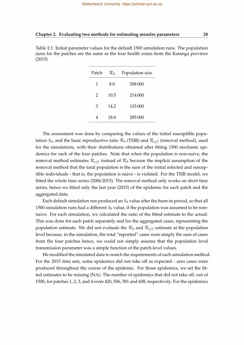
Chapter 2. Evaluating two methods for estimating measles parameters 28
Table 2.1: Initial parameter values for the default 1500 simulation runs. The populationsizes for the patches are the same as the four health zones from the Katanga province(2015).
Patch R0 Population size
1 8.0 308 000
2 10.5 214 000
3 14.2 133 000
4 18.8 285 000
The assessment was done by comparing the values of the initial susceptible popu-lation S0, and the basic reproductive ratio R0 (TSIR) and Re f f (removal method), usedfor the simulations, with their distributions obtained after fitting 1500 stochastic epi-demics for each of the four patches. Note that when the population is non-naive, theremoval method estimates Re f f instead of R0 because the implicit assumption of theremoval method that the total population is the sum of the initial infected and suscep-tible individuals - that is, the population is naive - is violated. For the TSIR model, wefitted the whole time series (2006-2015). The removal method only works on short timeseries, hence we fitted only the last year (2015) of the epidemic for each patch and theaggregated data.
Each default simulation run produced an S0 value after the burn-in period, so that all1500 simulation runs had a different S0 value, if the population was assumed to be non-naive. For each simulation, we calculated the ratio of the fitted estimate to the actual.This was done for each patch separately and for the aggregated cases, representing thepopulation estimate. We did not evaluate the R0 and Re f f estimate at the populationlevel because, in the simulation, the total “reported” cases were simply the sum of casesfrom the four patches hence, we could not simply assume that the population leveltransmission parameter was a simple function of the patch-level values.
We modified the simulated data to match the requirements of each simulation method.For the 2015 data sets, some epidemics did not take off as expected - zero cases wereproduced throughout the course of the epidemic. For those epidemics, we set the fit-ted estimates to be missing (NA). The number of epidemics that did not take off, out of1500, for patches 1, 2, 3, and 4 were 420, 506, 581 and 608, respectively. For the epidemics
Stellenbosch University https://scholar.sun.ac.za
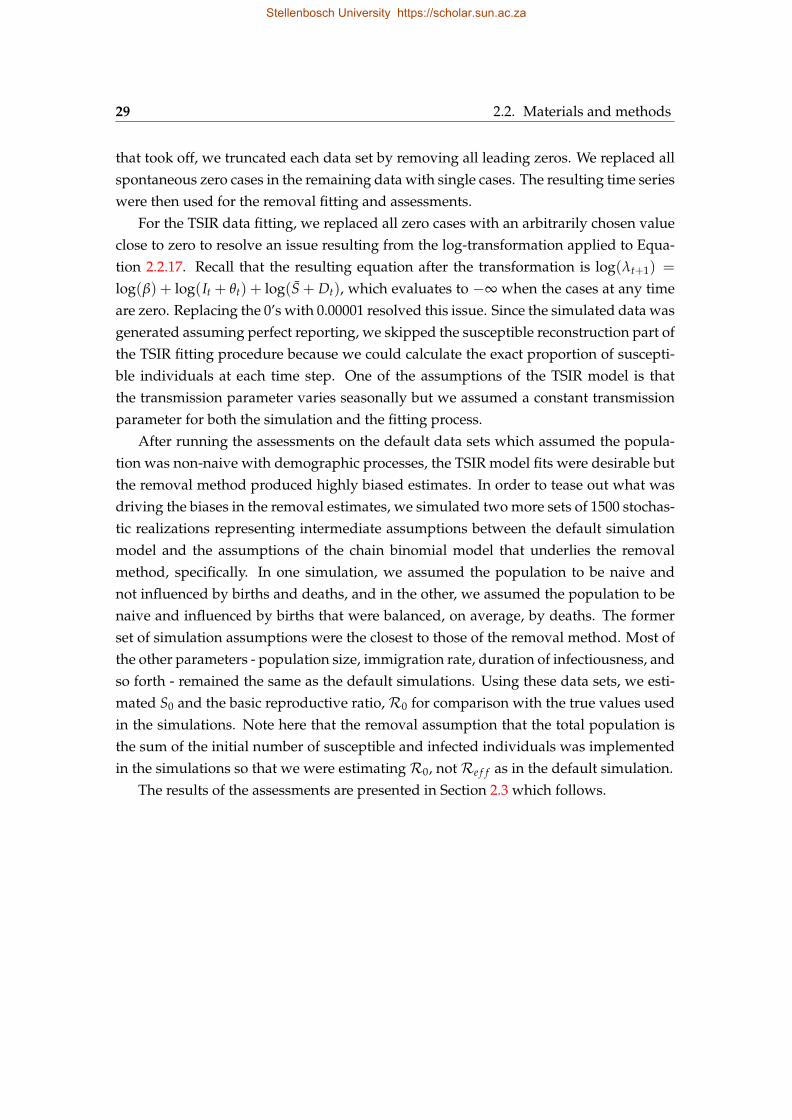
29 2.2. Materials and methods
that took off, we truncated each data set by removing all leading zeros. We replaced allspontaneous zero cases in the remaining data with single cases. The resulting time serieswere then used for the removal fitting and assessments.
For the TSIR data fitting, we replaced all zero cases with an arbitrarily chosen valueclose to zero to resolve an issue resulting from the log-transformation applied to Equa-tion 2.2.17. Recall that the resulting equation after the transformation is log(λt+1) =
log(β) + log(It + θt) + log(S + Dt), which evaluates to −∞ when the cases at any timeare zero. Replacing the 0’s with 0.00001 resolved this issue. Since the simulated data wasgenerated assuming perfect reporting, we skipped the susceptible reconstruction part ofthe TSIR fitting procedure because we could calculate the exact proportion of suscepti-ble individuals at each time step. One of the assumptions of the TSIR model is thatthe transmission parameter varies seasonally but we assumed a constant transmissionparameter for both the simulation and the fitting process.
After running the assessments on the default data sets which assumed the popula-tion was non-naive with demographic processes, the TSIR model fits were desirable butthe removal method produced highly biased estimates. In order to tease out what wasdriving the biases in the removal estimates, we simulated two more sets of 1500 stochas-tic realizations representing intermediate assumptions between the default simulationmodel and the assumptions of the chain binomial model that underlies the removalmethod, specifically. In one simulation, we assumed the population to be naive andnot influenced by births and deaths, and in the other, we assumed the population to benaive and influenced by births that were balanced, on average, by deaths. The formerset of simulation assumptions were the closest to those of the removal method. Most ofthe other parameters - population size, immigration rate, duration of infectiousness, andso forth - remained the same as the default simulations. Using these data sets, we esti-mated S0 and the basic reproductive ratio,R0 for comparison with the true values usedin the simulations. Note here that the removal assumption that the total population isthe sum of the initial number of susceptible and infected individuals was implementedin the simulations so that we were estimatingR0, notRe f f as in the default simulation.
The results of the assessments are presented in Section 2.3 which follows.
Stellenbosch University https://scholar.sun.ac.za
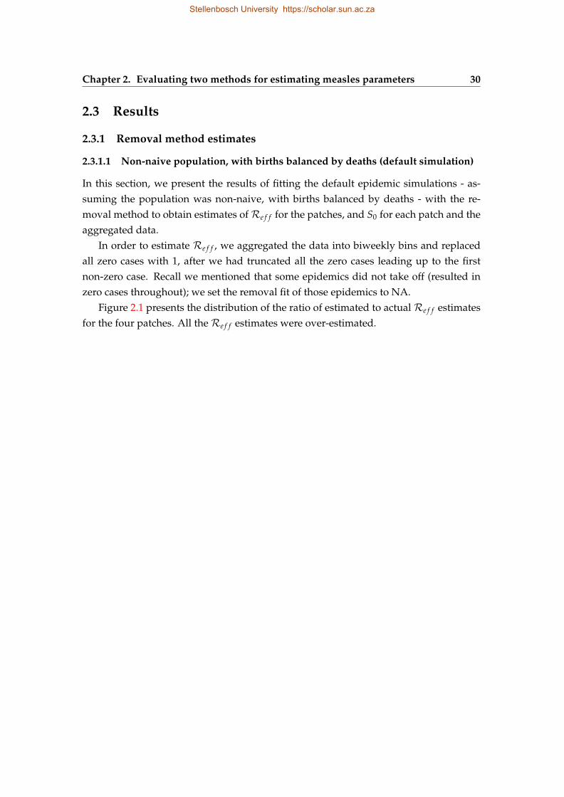
Chapter 2. Evaluating two methods for estimating measles parameters 30
2.3 Results
2.3.1 Removal method estimates
2.3.1.1 Non-naive population, with births balanced by deaths (default simulation)
In this section, we present the results of fitting the default epidemic simulations - as-suming the population was non-naive, with births balanced by deaths - with the re-moval method to obtain estimates ofRe f f for the patches, and S0 for each patch and theaggregated data.
In order to estimate Re f f , we aggregated the data into biweekly bins and replacedall zero cases with 1, after we had truncated all the zero cases leading up to the firstnon-zero case. Recall we mentioned that some epidemics did not take off (resulted inzero cases throughout); we set the removal fit of those epidemics to NA.
Figure 2.1 presents the distribution of the ratio of estimated to actual Re f f estimatesfor the four patches. All theRe f f estimates were over-estimated.
Stellenbosch University https://scholar.sun.ac.za
31 2.3. Results
0
200
400
600
0 100 200 300 400
relative Reff
coun
t
0
100
200
300
400
500
0 50 100 150
relative Reff
coun
t
0
100
200
300
400
0 50 100 150 200
relative Reff
coun
t
0
100
200
300
0 25 50 75 100
relative Reff
coun
t
Figure 2.1: Ratio of estimated to actual Re f f values for four patches, using the removalmethod. The simulation assumes each patch has a non-naive population with a constantbirth rate balanced out by the death rate - this was the default simulation - but theremoval method assumes the population to be naive, without births and deaths. Theassumptions of the data generation process and the removal method do not match inthis case. The number of epidemics that did not take off for patches 1, 2, 3, and 4 were420, 506, 581 and 608, respectively. The plots are arranged from top left to bottom rightaccording to patch 1, patch 2, patch 3, and patch 4, respectively. The reference point isat 1 on the x-axis. Notice that the axes are not on the same scale.
Table 2.2 below shows a summary of the results of the ratio of estimated to actualRe f f values across the four patches in terms of mean and median.
Stellenbosch University https://scholar.sun.ac.za
Chapter 2. Evaluating two methods for estimating measles parameters 32
Table 2.2: Median and mean of the ratio of the estimated to actual Re f f for the fourpatches, using the removal method. The simulation assumes the population is non-naive, with births balanced by deaths. All theRe f f estimates were biased high.
Patch 1 Patch 2 Patch 3 Patch 4
Median 5.12 5.00 7.12 3.46
Mean 7.87 8.31 11.64 6.17
In Figure 2.2 which follows, we show the distribution of the ratio of the estimated toactual S0 values for the four patches. It is clear that S0 was over-estimated in all patches.
0
100
200
300
0.0 2.5 5.0 7.5 10.0
relative S0
coun
t
0
100
200
300
0 2 4 6 8 10 12 14 16 18
relative S0
coun
t
0
100
200
300
0 8 16 24 32 40 48 56 64
relative S0
coun
t
0
100
200
0 8 16 24 32 40 48 56 64 72
relative S0
coun
t
Figure 2.2: Ratio of estimated to actual S0 values, for the four patches, using the removalmethod. The simulation assumes that each patch has a non-naive population with con-stant births, balanced by deaths, contrary to the assumptions of the removal methodthat the population is naive, without births and deaths. The number of epidemics thatdid not take off for patches 1, 2, 3, and 4 were 420, 506, 581 and 608, respectively. Theplots are arranged from top left to bottom right according to patch 1, patch 2, patch 3,and patch 4, respectively. The reference point is at 1 on the x-axis. Notice that the axesare not on the same scale.
Stellenbosch University https://scholar.sun.ac.za
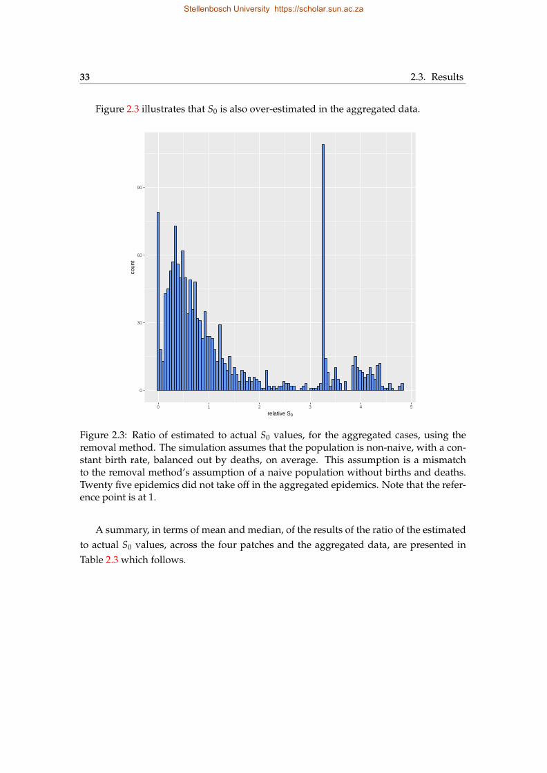
33 2.3. Results
Figure 2.3 illustrates that S0 is also over-estimated in the aggregated data.
0
30
60
90
0 1 2 3 4 5
relative S0
coun
t
Figure 2.3: Ratio of estimated to actual S0 values, for the aggregated cases, using theremoval method. The simulation assumes that the population is non-naive, with a con-stant birth rate, balanced out by deaths, on average. This assumption is a mismatchto the removal method’s assumption of a naive population without births and deaths.Twenty five epidemics did not take off in the aggregated epidemics. Note that the refer-ence point is at 1.
A summary, in terms of mean and median, of the results of the ratio of the estimatedto actual S0 values, across the four patches and the aggregated data, are presented inTable 2.3 which follows.
Stellenbosch University https://scholar.sun.ac.za
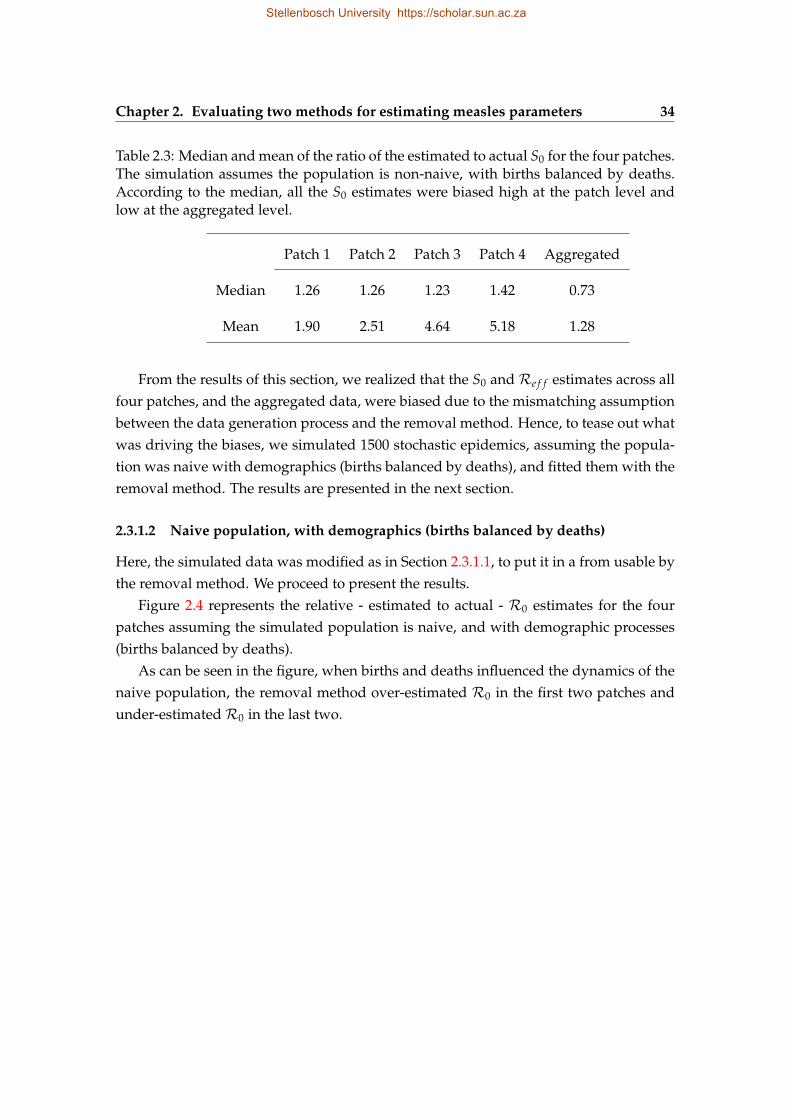
Chapter 2. Evaluating two methods for estimating measles parameters 34
Table 2.3: Median and mean of the ratio of the estimated to actual S0 for the four patches.The simulation assumes the population is non-naive, with births balanced by deaths.According to the median, all the S0 estimates were biased high at the patch level andlow at the aggregated level.
Patch 1 Patch 2 Patch 3 Patch 4 Aggregated
Median 1.26 1.26 1.23 1.42 0.73
Mean 1.90 2.51 4.64 5.18 1.28
From the results of this section, we realized that the S0 and Re f f estimates across allfour patches, and the aggregated data, were biased due to the mismatching assumptionbetween the data generation process and the removal method. Hence, to tease out whatwas driving the biases, we simulated 1500 stochastic epidemics, assuming the popula-tion was naive with demographics (births balanced by deaths), and fitted them with theremoval method. The results are presented in the next section.
2.3.1.2 Naive population, with demographics (births balanced by deaths)
Here, the simulated data was modified as in Section 2.3.1.1, to put it in a from usable bythe removal method. We proceed to present the results.
Figure 2.4 represents the relative - estimated to actual - R0 estimates for the fourpatches assuming the simulated population is naive, and with demographic processes(births balanced by deaths).
As can be seen in the figure, when births and deaths influenced the dynamics of thenaive population, the removal method over-estimated R0 in the first two patches andunder-estimatedR0 in the last two.
Stellenbosch University https://scholar.sun.ac.za
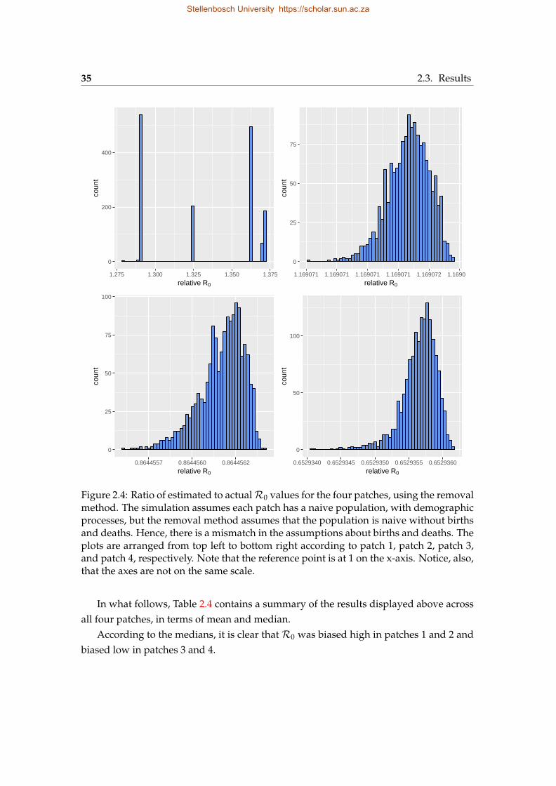
35 2.3. Results
0
200
400
1.275 1.300 1.325 1.350 1.375
relative R0
coun
t
0
25
50
75
1.169071 1.169071 1.169071 1.169071 1.169072 1.169072
relative R0co
unt
0
25
50
75
100
0.8644557 0.8644560 0.8644562
relative R0
coun
t
0
50
100
0.6529340 0.6529345 0.6529350 0.6529355 0.6529360
relative R0
coun
t
Figure 2.4: Ratio of estimated to actualR0 values for the four patches, using the removalmethod. The simulation assumes each patch has a naive population, with demographicprocesses, but the removal method assumes that the population is naive without birthsand deaths. Hence, there is a mismatch in the assumptions about births and deaths. Theplots are arranged from top left to bottom right according to patch 1, patch 2, patch 3,and patch 4, respectively. Note that the reference point is at 1 on the x-axis. Notice, also,that the axes are not on the same scale.
In what follows, Table 2.4 contains a summary of the results displayed above acrossall four patches, in terms of mean and median.
According to the medians, it is clear that R0 was biased high in patches 1 and 2 andbiased low in patches 3 and 4.
Stellenbosch University https://scholar.sun.ac.za
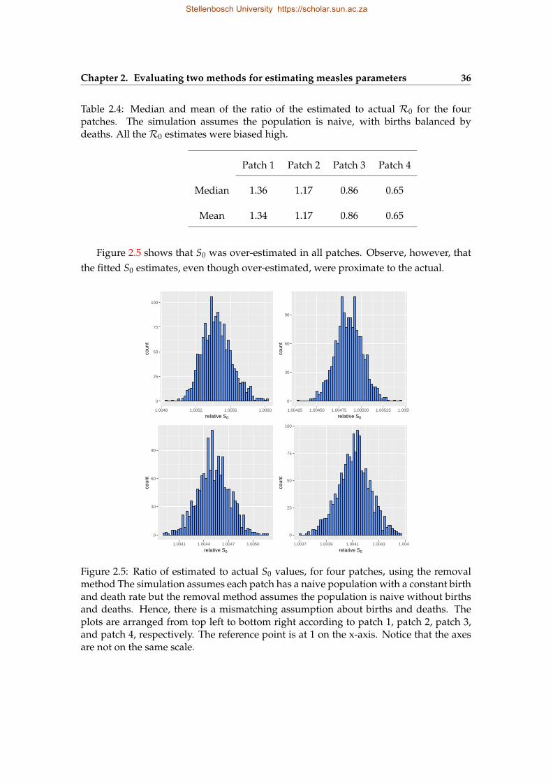
Chapter 2. Evaluating two methods for estimating measles parameters 36
Table 2.4: Median and mean of the ratio of the estimated to actual R0 for the fourpatches. The simulation assumes the population is naive, with births balanced bydeaths. All theR0 estimates were biased high.
Patch 1 Patch 2 Patch 3 Patch 4
Median 1.36 1.17 0.86 0.65
Mean 1.34 1.17 0.86 0.65
Figure 2.5 shows that S0 was over-estimated in all patches. Observe, however, thatthe fitted S0 estimates, even though over-estimated, were proximate to the actual.
0
25
50
75
100
1.0048 1.0052 1.0056 1.0060
relative S0
coun
t
0
30
60
90
1.00425 1.00450 1.00475 1.00500 1.00525 1.00550
relative S0
coun
t
0
30
60
90
1.0041 1.0044 1.0047 1.0050
relative S0
coun
t
0
25
50
75
100
1.0037 1.0039 1.0041 1.0043 1.0045
relative S0
coun
t
Figure 2.5: Ratio of estimated to actual S0 values, for four patches, using the removalmethod The simulation assumes each patch has a naive population with a constant birthand death rate but the removal method assumes the population is naive without birthsand deaths. Hence, there is a mismatching assumption about births and deaths. Theplots are arranged from top left to bottom right according to patch 1, patch 2, patch 3,and patch 4, respectively. The reference point is at 1 on the x-axis. Notice that the axesare not on the same scale.
Stellenbosch University https://scholar.sun.ac.za
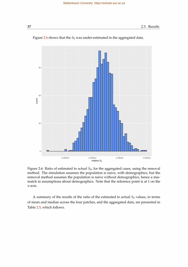
37 2.3. Results
Figure 2.6 shows that the S0 was under-estimated in the aggregated data.
0
30
60
90
0.006002 0.006003 0.006004 0.006005
relative S0
coun
t
Figure 2.6: Ratio of estimated to actual S0, for the aggregated cases, using the removalmethod. The simulation assumes the population is naive, with demographics, but theremoval method assumes the population is naive without demographics, hence a mis-match in assumptions about demographics. Note that the reference point is at 1 on thex-axis.
A summary of the results of the ratio of the estimated to actual S0 values, in termsof mean and median across the four patches, and the aggregated data, are presented inTable 2.5, which follows.
Stellenbosch University https://scholar.sun.ac.za
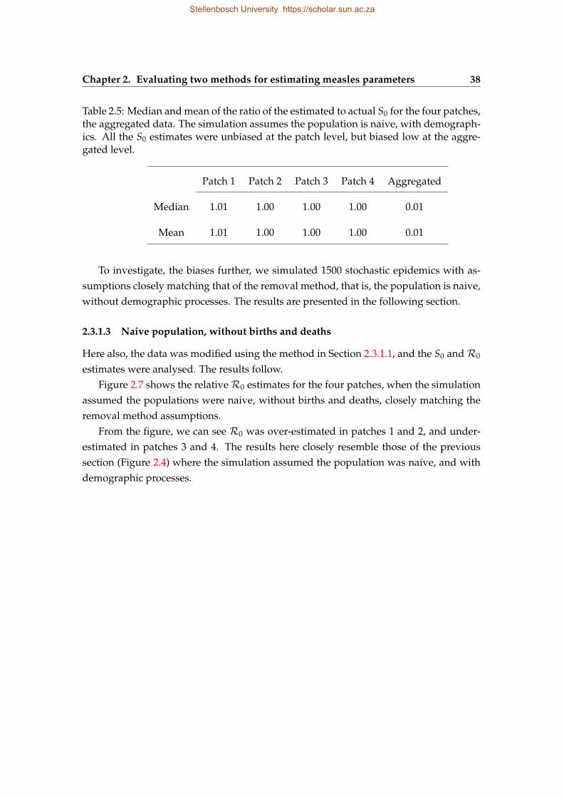
Chapter 2. Evaluating two methods for estimating measles parameters 38
Table 2.5: Median and mean of the ratio of the estimated to actual S0 for the four patches,the aggregated data. The simulation assumes the population is naive, with demograph-ics. All the S0 estimates were unbiased at the patch level, but biased low at the aggre-gated level.
Patch 1 Patch 2 Patch 3 Patch 4 Aggregated
Median 1.01 1.00 1.00 1.00 0.01
Mean 1.01 1.00 1.00 1.00 0.01
To investigate, the biases further, we simulated 1500 stochastic epidemics with as-sumptions closely matching that of the removal method, that is, the population is naive,without demographic processes. The results are presented in the following section.
2.3.1.3 Naive population, without births and deaths
Here also, the data was modified using the method in Section 2.3.1.1, and the S0 andR0
estimates were analysed. The results follow.Figure 2.7 shows the relativeR0 estimates for the four patches, when the simulation
assumed the populations were naive, without births and deaths, closely matching theremoval method assumptions.
From the figure, we can see R0 was over-estimated in patches 1 and 2, and under-estimated in patches 3 and 4. The results here closely resemble those of the previoussection (Figure 2.4) where the simulation assumed the population was naive, and withdemographic processes.
Stellenbosch University https://scholar.sun.ac.za
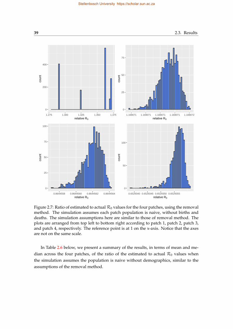
39 2.3. Results
0
200
400
1.275 1.300 1.325 1.350 1.375
relative R0
coun
t
0
25
50
75
1.169071 1.169071 1.169071 1.169071 1.169072
relative R0co
unt
0
25
50
75
100
0.8644558 0.8644560 0.8644562 0.8644564
relative R0
coun
t
0
50
100
0.6529340 0.6529345 0.6529350 0.6529355
relative R0
coun
t
Figure 2.7: Ratio of estimated to actualR0 values for the four patches, using the removalmethod. The simulation assumes each patch population is naive, without births anddeaths. The simulation assumptions here are similar to those of removal method. Theplots are arranged from top left to bottom right according to patch 1, patch 2, patch 3,and patch 4, respectively. The reference point is at 1 on the x-axis. Notice that the axesare not on the same scale.
In Table 2.6 below, we present a summary of the results, in terms of mean and me-dian across the four patches, of the ratio of the estimated to actual R0 values whenthe simulation assumes the population is naive without demographics, similar to theassumptions of the removal method.
Stellenbosch University https://scholar.sun.ac.za
Chapter 2. Evaluating two methods for estimating measles parameters 40
Table 2.6: Median and mean of the ratio of the estimated to actual R0 for the fourpatches. The simulation assumes the population is naive, without births and deaths,similar to the assumptions of the removal method. The R0 estimates were biased highin patches 1 and 2, and biased low in patches 3 and 4.
Patch 1 Patch 2 Patch 3 Patch 4
Median 1.33 1.17 0.86 0.65
Mean 1.33 1.17 0.86 0.65
Figure 2.8, illustrates the relative S0 estimates at the patch level. The estimates areunbiased since their relative ratios surround 1.
0
50
100
0.9999 1.0000 1.0001 1.0002 1.0003
relative S0
coun
t
0
50
100
150
200
250
1.00009 1.00011 1.00013 1.00015
relative S0
coun
t
0
200
400
600
1.000195 1.000200 1.000205 1.000210
relative S0
coun
t
0
100
200
1.000120 1.000122 1.000124
relative S0
coun
t
Figure 2.8: Ratio of estimated to actual S0 values, for the four patches, using the removalmethod. The simulation assumes that each patch has a naive population without demo-graphics. These assumptions are the closest to that of the removal method. The plots arearranged from top left to bottom right according to patch 1, patch 2, patch 3, and patch4, respectively. The reference point is at 1 on the x-axis. Notice that the axes are not onthe same scale.
Stellenbosch University https://scholar.sun.ac.za
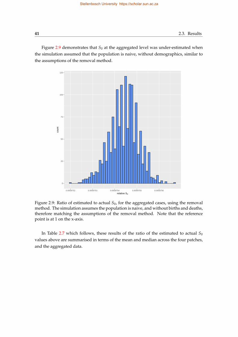
41 2.3. Results
Figure 2.9 demonstrates that S0 at the aggregated level was under-estimated whenthe simulation assumed that the population is naive, without demographics, similar tothe assumptions of the removal method.
0
25
50
75
100
125
0.0059752 0.0059753 0.0059754 0.0059755 0.0059756
relative S0
coun
t
Figure 2.9: Ratio of estimated to actual S0, for the aggregated cases, using the removalmethod. The simulation assumes the population is naive, and without births and deaths,therefore matching the assumptions of the removal method. Note that the referencepoint is at 1 on the x-axis.
In Table 2.7 which follows, these results of the ratio of the estimated to actual S0
values above are summarised in terms of the mean and median across the four patches,and the aggregated data.
Stellenbosch University https://scholar.sun.ac.za
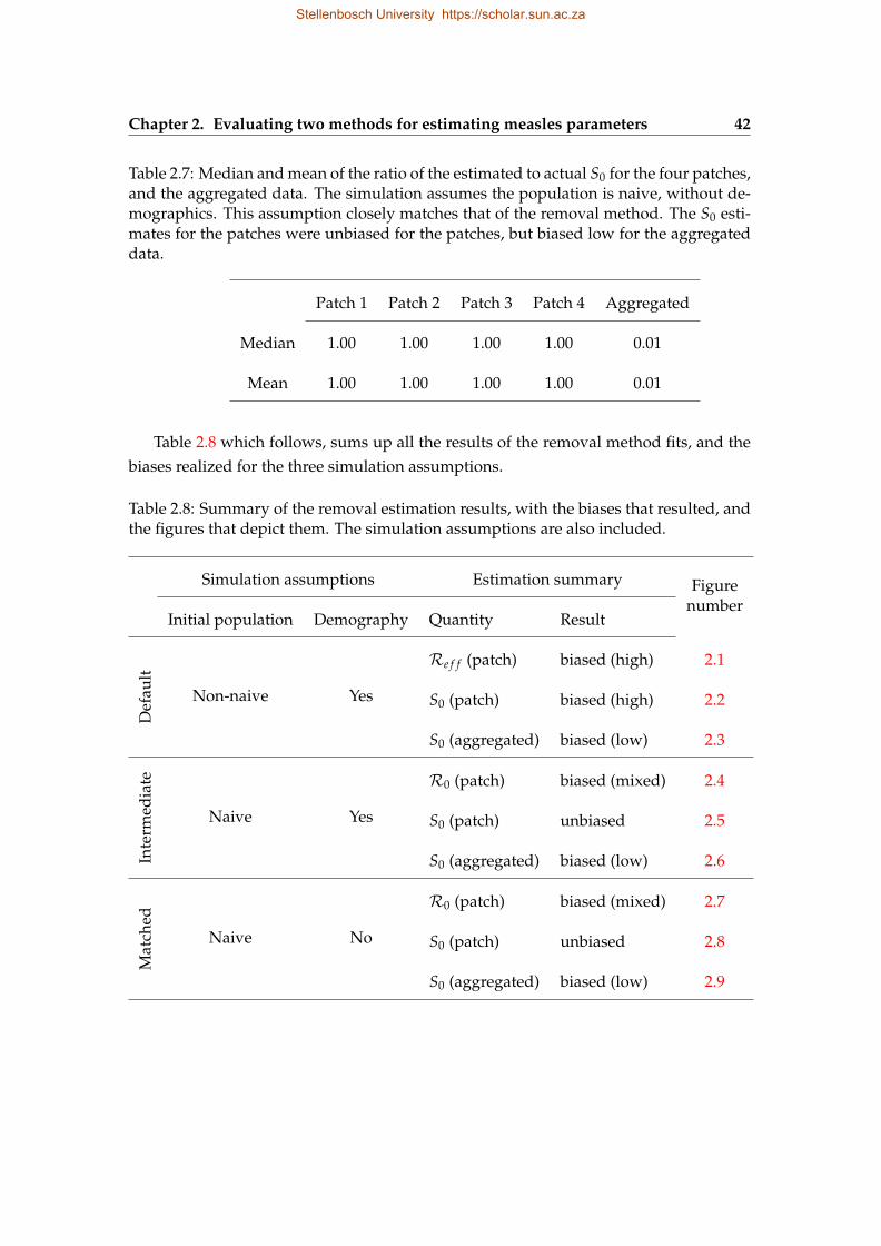
Chapter 2. Evaluating two methods for estimating measles parameters 42
Table 2.7: Median and mean of the ratio of the estimated to actual S0 for the four patches,and the aggregated data. The simulation assumes the population is naive, without de-mographics. This assumption closely matches that of the removal method. The S0 esti-mates for the patches were unbiased for the patches, but biased low for the aggregateddata.
Patch 1 Patch 2 Patch 3 Patch 4 Aggregated
Median 1.00 1.00 1.00 1.00 0.01
Mean 1.00 1.00 1.00 1.00 0.01
Table 2.8 which follows, sums up all the results of the removal method fits, and thebiases realized for the three simulation assumptions.
Table 2.8: Summary of the removal estimation results, with the biases that resulted, andthe figures that depict them. The simulation assumptions are also included.
Simulation assumptions Estimation summary Figurenumber
Initial population Demography Quantity Result
Def
ault
Non-naive Yes
Re f f (patch) biased (high) 2.1
S0 (patch) biased (high) 2.2
S0 (aggregated) biased (low) 2.3
Inte
rmed
iate
Naive Yes
R0 (patch) biased (mixed) 2.4
S0 (patch) unbiased 2.5
S0 (aggregated) biased (low) 2.6
Mat
ched
Naive No
R0 (patch) biased (mixed) 2.7
S0 (patch) unbiased 2.8
S0 (aggregated) biased (low) 2.9
Stellenbosch University https://scholar.sun.ac.za
43 2.3. Results
2.3.2 TSIR estimates
In this section, we present the results of fitting the default 1500 stochastic epidemics,each spanning the period between December 26, 2005 and December 28, 2015, with theTSIR model. Recall that for the default simulation, we assumed that the populationwas non-naive and that the population dynamics were influenced by births, which werebalanced out by deaths, on average.
Because we assumed perfect reporting in our simulations, the actual S0 value at thepatch level, were summed to yield the population-level S0 value to allow for compari-son with the fitted value. The R0 estimates were only fitted at the patch-level becausethe population-level R0 was not assumed to be the sum of R0 from the patches. TheTSIR model was only fitted to the default simulated epidemics because the simulationassumptions were similar to that of the TSIR model.
In the following section, we display the results of comparing the fitted S0 and R0
estimates to the actuals.
2.3.2.1 Non-naive population, with demographics (default simulation)
To estimateR0 from the default simulation data, we replaced all zero cases with a valueof 0.00001, then we aggregated the data into biweekly bins to match the time-step of theTSIR model.
From Figure 2.10, we observe in all four patches that R0 was biased low, since mostof the estimates lie to the left of the reference of 1 on the x-axis.
Stellenbosch University https://scholar.sun.ac.za
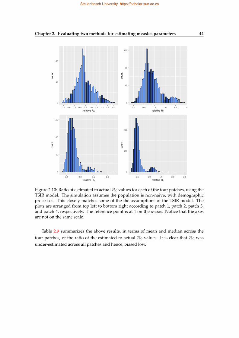
Chapter 2. Evaluating two methods for estimating measles parameters 44
0
50
100
0.5 0.6 0.7 0.8 0.9 1.0 1.1 1.2 1.3 1.4
relative R0
coun
t
0
40
80
120
0.4 0.6 0.8 1.0 1.2 1.4
relative R0
coun
t
0
50
100
150
0.4 0.8 1.2 1.6
relative R0
coun
t
0
100
200
0.5 1.0 1.5 2.0 2.5
relative R0
coun
t
Figure 2.10: Ratio of estimated to actualR0 values for each of the four patches, using theTSIR model. The simulation assumes the population is non-naive, with demographicprocesses. This closely matches some of the the assumptions of the TSIR model. Theplots are arranged from top left to bottom right according to patch 1, patch 2, patch 3,and patch 4, respectively. The reference point is at 1 on the x-axis. Notice that the axesare not on the same scale.
Table 2.9 summarizes the above results, in terms of mean and median across thefour patches, of the ratio of the estimated to actual R0 values. It is clear that R0 wasunder-estimated across all patches and hence, biased low.
Stellenbosch University https://scholar.sun.ac.za
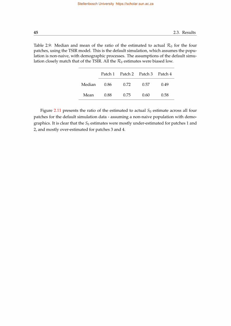
45 2.3. Results
Table 2.9: Median and mean of the ratio of the estimated to actual R0 for the fourpatches, using the TSIR model. This is the default simulation, which assumes the popu-lation is non-naive, with demographic processes. The assumptions of the default simu-lation closely match that of the TSIR. All theR0 estimates were biased low.
Patch 1 Patch 2 Patch 3 Patch 4
Median 0.86 0.72 0.57 0.49
Mean 0.88 0.75 0.60 0.58
Figure 2.11 presents the ratio of the estimated to actual S0 estimate across all fourpatches for the default simulation data - assuming a non-naive population with demo-graphics. It is clear that the S0 estimates were mostly under-estimated for patches 1 and2, and mostly over-estimated for patches 3 and 4.
Stellenbosch University https://scholar.sun.ac.za
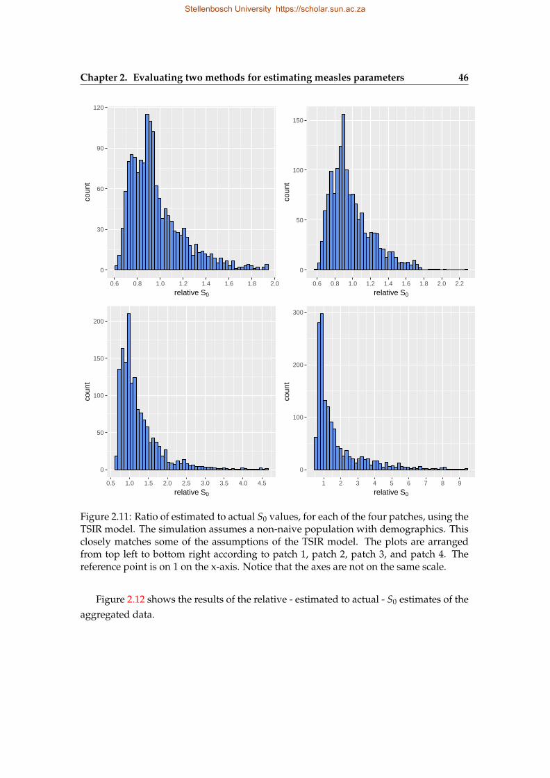
Chapter 2. Evaluating two methods for estimating measles parameters 46
0
30
60
90
120
0.6 0.8 1.0 1.2 1.4 1.6 1.8 2.0
relative S0
coun
t
0
50
100
150
0.6 0.8 1.0 1.2 1.4 1.6 1.8 2.0 2.2
relative S0
coun
t
0
50
100
150
200
0.5 1.0 1.5 2.0 2.5 3.0 3.5 4.0 4.5
relative S0
coun
t
0
100
200
300
1 2 3 4 5 6 7 8 9
relative S0
coun
t
Figure 2.11: Ratio of estimated to actual S0 values, for each of the four patches, using theTSIR model. The simulation assumes a non-naive population with demographics. Thisclosely matches some of the assumptions of the TSIR model. The plots are arrangedfrom top left to bottom right according to patch 1, patch 2, patch 3, and patch 4. Thereference point is on 1 on the x-axis. Notice that the axes are not on the same scale.
Figure 2.12 shows the results of the relative - estimated to actual - S0 estimates of theaggregated data.
Stellenbosch University https://scholar.sun.ac.za
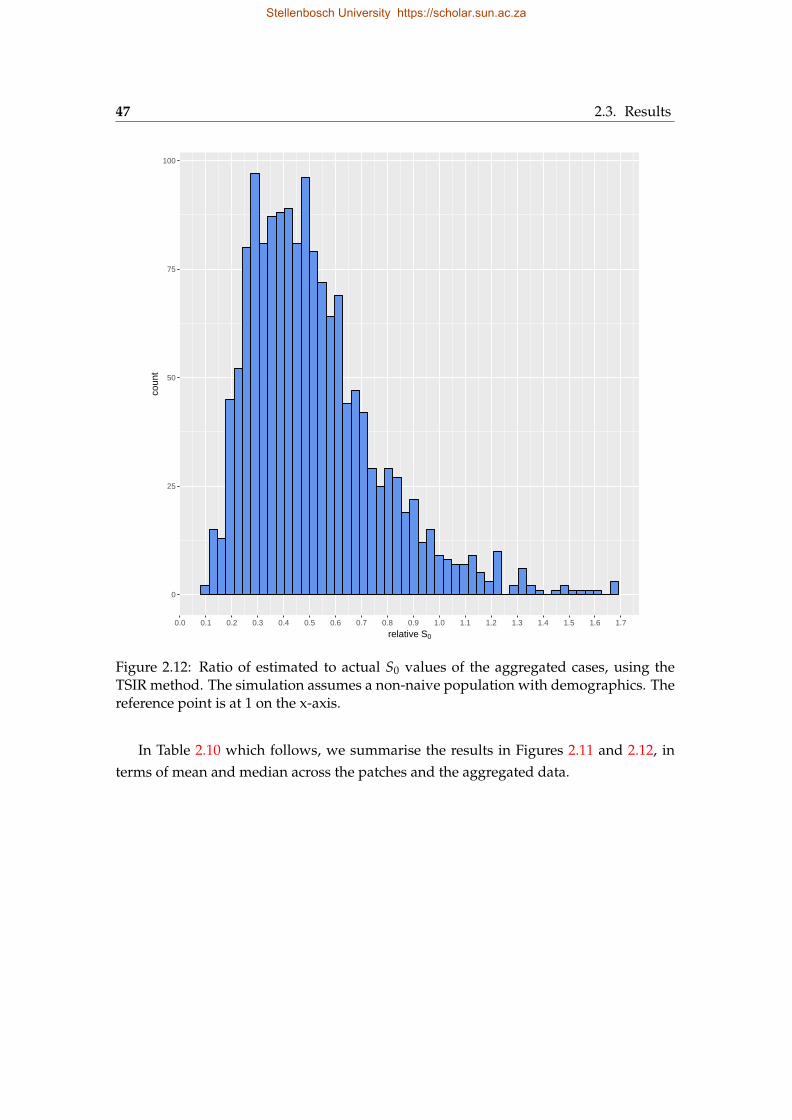
47 2.3. Results
0
25
50
75
100
0.0 0.1 0.2 0.3 0.4 0.5 0.6 0.7 0.8 0.9 1.0 1.1 1.2 1.3 1.4 1.5 1.6 1.7
relative S0
coun
t
Figure 2.12: Ratio of estimated to actual S0 values of the aggregated cases, using theTSIR method. The simulation assumes a non-naive population with demographics. Thereference point is at 1 on the x-axis.
In Table 2.10 which follows, we summarise the results in Figures 2.11 and 2.12, interms of mean and median across the patches and the aggregated data.
Stellenbosch University https://scholar.sun.ac.za
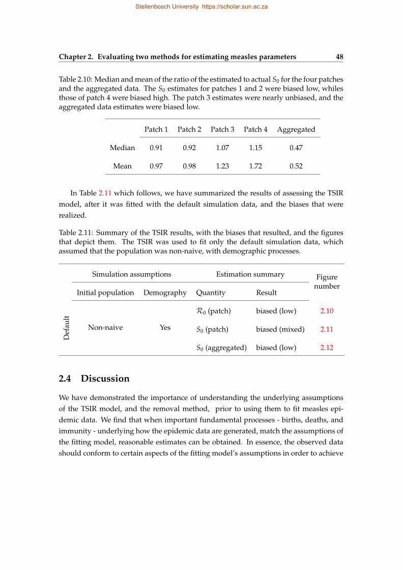
Chapter 2. Evaluating two methods for estimating measles parameters 48
Table 2.10: Median and mean of the ratio of the estimated to actual S0 for the four patchesand the aggregated data. The S0 estimates for patches 1 and 2 were biased low, whilesthose of patch 4 were biased high. The patch 3 estimates were nearly unbiased, and theaggregated data estimates were biased low.
Patch 1 Patch 2 Patch 3 Patch 4 Aggregated
Median 0.91 0.92 1.07 1.15 0.47
Mean 0.97 0.98 1.23 1.72 0.52
In Table 2.11 which follows, we have summarized the results of assessing the TSIRmodel, after it was fitted with the default simulation data, and the biases that wererealized.
Table 2.11: Summary of the TSIR results, with the biases that resulted, and the figuresthat depict them. The TSIR was used to fit only the default simulation data, whichassumed that the population was non-naive, with demographic processes.
Simulation assumptions Estimation summary Figurenumber
Initial population Demography Quantity Result
Def
ault
Non-naive Yes
R0 (patch) biased (low) 2.10
S0 (patch) biased (mixed) 2.11
S0 (aggregated) biased (low) 2.12
2.4 Discussion
We have demonstrated the importance of understanding the underlying assumptionsof the TSIR model, and the removal method, prior to using them to fit measles epi-demic data. We find that when important fundamental processes - births, deaths, andimmunity - underlying how the epidemic data are generated, match the assumptions ofthe fitting model, reasonable estimates can be obtained. In essence, the observed datashould conform to certain aspects of the fitting model’s assumptions in order to achieve
Stellenbosch University https://scholar.sun.ac.za
49 2.4. Discussion
reasonable estimates. It is interesting to know that the fitting is robust to some differ-ences in assumptions, especially in terms of the duration of infection, and the modeltime-step.
This result was facilitated by running stochastic epidemic simulations, with varyingassumptions about the occurrence of births and deaths, and whether the population wasnaive or not. This study only confirms the utility of simulations as a powerful tool forpursuing scientific enquiries. Simulations are a useful tool for investigating inquiriessurrounding various phenomena. Refer to Bellan et al. (2015), Halloran et al. (2017), andLessler et al. (2016) for examples of cases in which simulations were employed to answerpertinent questions in mathematical epidemiology.
The amount of bias surrounding both the TSIR and removal S0 estimates at the ag-gregated level, compared to the patch level, is striking. This seems to suggest that pa-rameter fits on data at an aggregated scale tend to have higher amounts of uncertaintycompared to data reported at a finer spatial scale. Hence, statistical inference done withfitted estimates of aggregated data should be interpreted with cognisance of the poten-tial biases resulting from aggregation. Even though we assumed perfect reporting inour simulations, the aggregated data produced more biased S0 estimates than the seg-regated patch data. It is, therefore, interesting to imagine the amount of bias that couldresult from actual epidemics, knowing they are often aggregated and also affected byissues such as under-reporting (Bobashev et al., 2000).
Several reasons could explain the biases surrounding the removal estimates. The bi-ases are driven by whether the population being fitted is naive or not - estimates from thenon-naive populations are highly biased compared to those from the naive populations,irrespective of assumptions about the occurrence of demographic processes. In their pa-per, Ferrari et al. (2005) indicated that the removal estimator’s performance is affectedby the depleting susceptible population along the course of the epidemic - the methodassumes there is no susceptible recruitment through birth, due to the fast progression ofthe epidemic. Hence, applying the model to the full course of a long epidemic could beproblematic. This could be one reason behind the biases observed since we applied themethod to the 2015 time series, beginning from the first occurrence of non-zero cases onthe epidemic trajectory. Additionally, the removal method does not work on data thathas spontaneous zeros. This assumption is difficult to adhere to, especially consideringthe fact that when the observed data is segregated at a fine spatial scale, zero cases areprevalent. When we replace all zero cases with 1’s to resolve this issue, it potentiallybiased the expectedR0 as depicted in Figure 2.7. However, the S0 estimates at the patchlevel tend to be unaffected by this fix since they remain unbiased, but are biased low at
Stellenbosch University https://scholar.sun.ac.za
Chapter 2. Evaluating two methods for estimating measles parameters 50
the aggregated level, as can be seen in Figures 2.9 and 2.8. The biases in the fitted S0
estimates are very little, compared with those ofR0 andRe f f .Some of the removal estimates were occasionally large, relative to the cluster of es-
timates. Our preliminary investigation reveals that these outliers occurred when theepidemic had a single peak, or when the epidemic did not take off. We will be investi-gating this further in the future.
The approach of replacing zero cases with 1’s is barely one out of many potential“fixes”. Other approaches could include any attempt at making sure all cases are non-zero, including “zooming” in to the part of the epidemic with a continuous successionof non-zero cases. In implementing such “fixes”, attempts should be made to quantifythe potential consequential biases.
The TSIR model estimates of S0 are distributed around the reference point of 1, sothat at the patch level, they are a mix of biases - patches 1 and 2 are biased low, patch 3is unbiased, and patch 4 is biased high, but all are close to 1 - but at the aggregated level,they are biased low. The R0 estimates are biased low for all the patches. These biasescould have been introduced when we replaced zero cases with a value close to zero.This “fix”, however, had a marginal magnitude of bias on S0 than it did on R0 - sinceit only partially increased the number of cases in the data, as confirmed by the results.One way to avoid this fix is to employ a Bayesian framework in the parametrizing theTSIR (Ferrari et al., 2008), instead of the linear regression method which employs thelog-transformation, disallowing for zero cases in the data.
When some of the assumptions underlying the data generation process closely matchedthe assumptions of the estimation model, the two models predicted S0 better at the patchlevel than at the population level, with the removal S0 estimate being proximate to theactual simulation values - for the naive populations. The TSIR predicted low biased es-timates of R0, whiles the removal method over-estimated (produced high biased) Re f f
estimates for the non-naive populations. When we teased out what was driving the biasin the removal method, it became clear that the assumption of naiveness in the popula-tion was a major driver - the method produced a mix of biased estimates of R0 and S0
for the naive populations, which were relatively better - to an order of magnitude - thanthe estimates obtained from the non-naive populations.
The results of this study should be interpreted with caution. It is our belief thateach different artificial modification of the time series that may be necessary to use anestimation method may produce different biases in magnitude and direction. Also, sincethe processes may differ significantly between those underlying how the actual data isgenerated and the simulated data, this exercise could be more complicated than what
Stellenbosch University https://scholar.sun.ac.za
51 2.4. Discussion
we have presented here.We have provided insights into the performance of the TSIR model in terms of the
biases produced, when a non-naive population, influenced by demographic processes,is fitted with the model to obtain estimates of R0 and S0. We have also provided thesame information regarding the removal fits of Re f f or R0, and S0 from three differentkinds of populations: non-naive, with births, balanced by deaths; naive, with births,balanced by deaths; naive, without births and deaths. It is evident that the performanceof the TSIR model and removal method depends on which important assumptions arematched between the estimation model and the data, the degree of aggregation of thedata, the artificial modifications made to the data to put it in a format usable by theestimation method, and the parameters being estimated.
In summary, the insights to be drawn from this chapter are that: violations of certaincore assumptions of the estimation model - for instance, the use of the removal methodto fit data from non-naive populations with high birth and death rates - can lead tobiased estimates being produced; parameter estimates appear fairly robust to simplemodifications of the time series, such as, replacing zero cases with 1s, for use with theremoval method, or replacing zero cases with small numbers, for use with the TSIRmethod. As to whether these findings hold when data are imperfectly reported remainsto be investigated.
Stellenbosch University https://scholar.sun.ac.za
Chapter 3
Measles outbreak in a high school inSouth Africa: assessing the impact ofa reactive vaccination campaign
3.1 Introduction
In February 2017 a measles outbreak was declared in Stellenbosch, South Africa, afterfive cases were detected in an all-boys high school. According to the South African De-partment of Health, the occurrence of five laboratory-confirmed measles cases warrantsthe declaration of an outbreak in the affected area. A day after the outbreak was de-clared, a non-selective reactive vaccination campaign was kick-started and more than93% of students within the school were vaccinated in a day.
As earlier mentioned in Chapter 1, assessing the impact of a vaccination campaign isessential for improving future campaigns. One common method of appraising a vacci-nation campaign is to quantify the cases averted. Accordingly, following the vaccinationcampaign at the high school, our study seeks to assess its impact using the same metric.
Also, whiles the outbreak was ongoing, it was in the interest of the stakeholders -the school authorities, the learners, and the learners’ parents - to know how many morecases were expected, and what time remained for the epidemic to subside followingthe campaign. This was important for two reasons: (1) the stakeholders needed somereassurance, and (2) plans needed to be made towards resuming the school’s activitieswhich were put on hold because of the outbreak. This study, therefore, aimed at pro-viding information pertaining to the epidemic progression in terms of cases and timeremaining until the epidemic ended.
52
Stellenbosch University https://scholar.sun.ac.za

53 3.2. Materials and methods
In the past, dynamical models have been a useful tool for estimating the aforemen-tioned quantities to assess the impact of vaccination programs - Examples of such stud-ies are Ferrari et al. (2014); Grais et al. (2007); Pinner et al. (1992) - hence, we developedand used a dynamical model for closed populations to achieve the set objectives.
3.2 Materials and methods
This section describes the model and methods employed to simulate the measles epi-demic as well as the data employed for the model validation.
3.2.1 Data description
3.2.1.1 A measles outbreak in a school in Stellenbosch, South Africa.
On January 15, 2017, Paul Roos Gymnasium, an all-boys high school in Stellenbosch,South Africa, recorded a case of measles. Following the first case, five secondary caseswere reported by January 31. This prompted the declaration of an outbreak on February2, by the Department of Health in the Western Cape Province. As a consequence, avaccination campaign was held on February 3, 2017 and more than 93% of the 1200learners at the school were vaccinated. By February 6, the number of lab-confirmedcases among the learners had risen to a total of 23. Subsequently, no new cases werereported. The epidemic in the school, therefore, lasted for about 22 days.
3.2.1.2 Outbreaks in other schools
To validate the model we formulated, we used comparable data sets obtained from pub-lished epidemics from five other schools. A description of each epidemic is given below.
The first is an outbreak in School A, Oxford, in 1929. The total number of studentswas 56, of which there were 36 susceptible students. The remaining 20 students had hadmeasles previously. Since there was no measles vaccine then, all the susceptible studentswere eventually infected by two students who got infected after illegally visiting theschool kitchen and contracting the infection from the cook. The outbreak lasted for 47days (Hobson, 1934).
In 1930, an outbreak occurred in School B, Oxford. This school had 121 students,of which 68 were susceptible. Out of this number, 48 acquired the infection and 20remained uninfected. The total epidemic duration was 49 days (Hobson, 1934).
Another outbreak occurred in School B, Oxford, in 1934. The total students were99 with 48 having previously been infected. The remaining 51 students were therefore
Stellenbosch University https://scholar.sun.ac.za
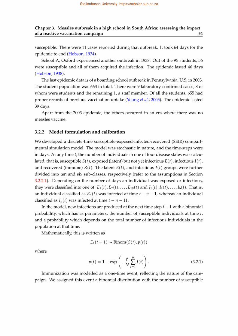
Chapter 3. Measles outbreak in a high school in South Africa: assessing the impactof a reactive vaccination campaign 54
susceptible. There were 11 cases reported during that outbreak. It took 64 days for theepidemic to end (Hobson, 1934).
School A, Oxford experienced another outbreak in 1938. Out of the 95 students, 56were susceptible and all of them acquired the infection. The epidemic lasted 46 days(Hobson, 1938).
The last epidemic data is of a boarding school outbreak in Pennsylvania, U.S, in 2003.The student population was 663 in total. There were 9 laboratory-confirmed cases, 8 ofwhom were students and the remaining 1, a staff member. Of all the students, 655 hadproper records of previous vaccination uptake (Yeung et al., 2005). The epidemic lasted39 days.
Apart from the 2003 epidemic, the others occurred in an era where there was nomeasles vaccine.
3.2.2 Model formulation and calibration
We developed a discrete-time susceptible-exposed-infected-recovered (SEIR) compart-mental simulation model. The model was stochastic in nature, and the time-steps werein days. At any time t, the number of individuals in one of four disease states was calcu-lated, that is, susceptible S(t), exposed (latent) but not yet infectious E(t), infectious I(t),and recovered (immune) R(t). The latent E(t), and infectious I(t) groups were furtherdivided into ten and six sub-classes, respectively (refer to the assumptions in Section3.2.2.1). Depending on the number of days an individual was exposed or infectious,they were classified into one of: E1(t), E2(t), . . . , E10(t) and I1(t), I2(t), . . . , I6(t). That is,an individual classified as En(t) was infected at time t− n − 1, whereas an individualclassified as In(t) was infected at time t− n− 11.
In the model, new infections are produced at the next time step t + 1 with a binomialprobability, which has as parameters, the number of susceptible individuals at time t,and a probability which depends on the total number of infectious individuals in thepopulation at that time.
Mathematically, this is written as
E1(t + 1) ∼ Binom(S(t), p(t))
where
p(t) = 1− exp
(− β
N
6
∑t=1
I(t)
). (3.2.1)
Immunization was modelled as a one-time event, reflecting the nature of the cam-paign. We assigned this event a binomial distribution with the number of susceptible
Stellenbosch University https://scholar.sun.ac.za
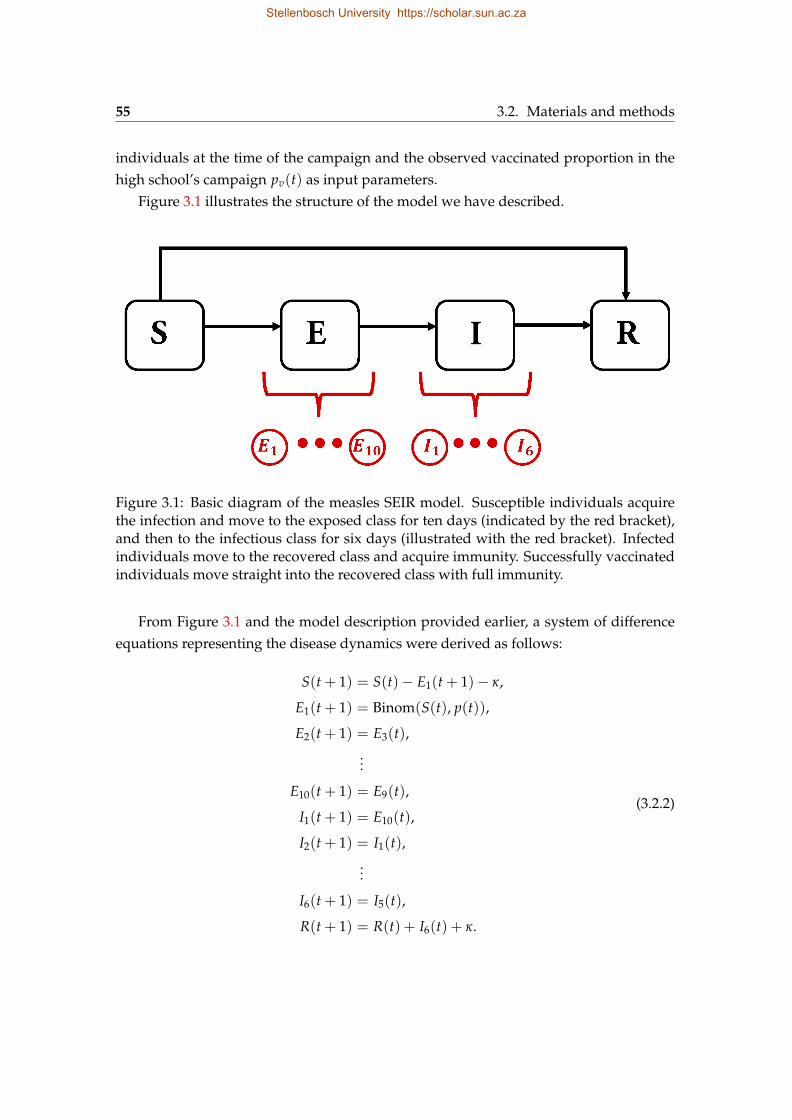
55 3.2. Materials and methods
individuals at the time of the campaign and the observed vaccinated proportion in thehigh school’s campaign pv(t) as input parameters.
Figure 3.1 illustrates the structure of the model we have described.
Figure 3.1: Basic diagram of the measles SEIR model. Susceptible individuals acquirethe infection and move to the exposed class for ten days (indicated by the red bracket),and then to the infectious class for six days (illustrated with the red bracket). Infectedindividuals move to the recovered class and acquire immunity. Successfully vaccinatedindividuals move straight into the recovered class with full immunity.
From Figure 3.1 and the model description provided earlier, a system of differenceequations representing the disease dynamics were derived as follows:
S(t + 1) = S(t)− E1(t + 1)− κ,
E1(t + 1) = Binom(S(t), p(t)),
E2(t + 1) = E3(t),...
E10(t + 1) = E9(t),
I1(t + 1) = E10(t),
I2(t + 1) = I1(t),...
I6(t + 1) = I5(t),
R(t + 1) = R(t) + I6(t) + κ.
(3.2.2)
Stellenbosch University https://scholar.sun.ac.za
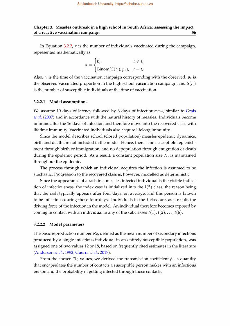
Chapter 3. Measles outbreak in a high school in South Africa: assessing the impactof a reactive vaccination campaign 56
In Equation 3.2.2, κ is the number of individuals vaccinated during the campaign,represented mathematically as
κ =
0, t 6= tc
Binom(S(tc), pv), t = tc
Also, tc is the time of the vaccination campaign corresponding with the observed, pv isthe observed vaccinated proportion in the high school vaccination campaign, and S(tc)
is the number of susceptible individuals at the time of vaccination.
3.2.2.1 Model assumptions
We assume 10 days of latency followed by 6 days of infectiousness, similar to Graiset al. (2007) and in accordance with the natural history of measles. Individuals becomeimmune after the 16 days of infection and therefore move into the recovered class withlifetime immunity. Vaccinated individuals also acquire lifelong immunity.
Since the model describes school (closed population) measles epidemic dynamics,birth and death are not included in the model. Hence, there is no susceptible replenish-ment through birth or immigration, and no depopulation through emigration or deathduring the epidemic period. As a result, a constant population size N, is maintainedthroughout the epidemic.
The process through which an individual acquires the infection is assumed to bestochastic. Progression to the recovered class is, however, modelled as deterministic.
Since the appearance of a rash in a measles-infected individual is the visible indica-tion of infectiousness, the index case is initialized into the I(5) class, the reason beingthat the rash typically appears after four days, on average, and this person is knownto be infectious during those four days. Individuals in the I class are, as a result, thedriving force of the infection in the model. An individual therefore becomes exposed bycoming in contact with an individual in any of the subclasses I(1), I(2), . . . , I(6).
3.2.2.2 Model parameters
The basic reproduction numberR0, defined as the mean number of secondary infectionsproduced by a single infectious individual in an entirely susceptible population, wasassigned one of two values 12 or 18, based on frequently cited estimates in the literature(Anderson et al., 1992; Guerra et al., 2017).
From the chosen R0 values, we derived the transmission coefficient β - a quantitythat encapsulates the number of contacts a susceptible person makes with an infectiousperson and the probability of getting infected through those contacts.
Stellenbosch University https://scholar.sun.ac.za
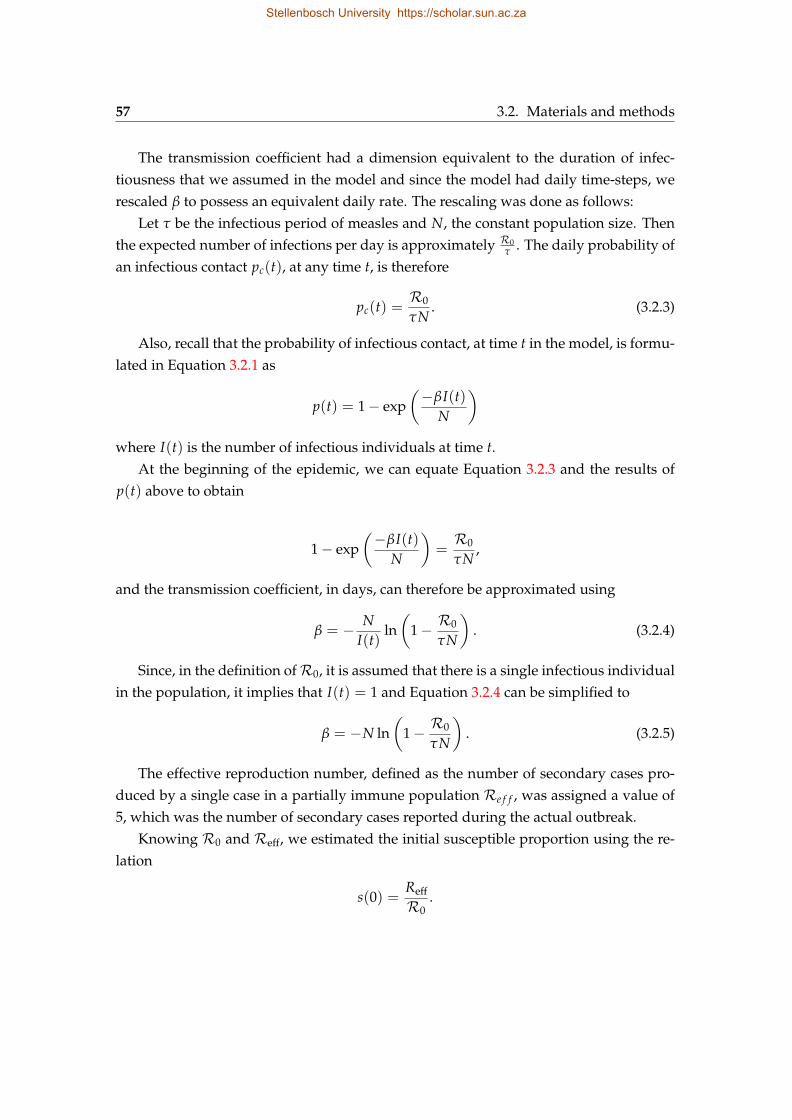
57 3.2. Materials and methods
The transmission coefficient had a dimension equivalent to the duration of infec-tiousness that we assumed in the model and since the model had daily time-steps, werescaled β to possess an equivalent daily rate. The rescaling was done as follows:
Let τ be the infectious period of measles and N, the constant population size. Thenthe expected number of infections per day is approximately R0
τ . The daily probability ofan infectious contact pc(t), at any time t, is therefore
pc(t) =R0
τN. (3.2.3)
Also, recall that the probability of infectious contact, at time t in the model, is formu-lated in Equation 3.2.1 as
p(t) = 1− exp(−βI(t)
N
)where I(t) is the number of infectious individuals at time t.
At the beginning of the epidemic, we can equate Equation 3.2.3 and the results ofp(t) above to obtain
1− exp(−βI(t)
N
)=R0
τN,
and the transmission coefficient, in days, can therefore be approximated using
β = − NI(t)
ln(
1− R0
τN
). (3.2.4)
Since, in the definition ofR0, it is assumed that there is a single infectious individualin the population, it implies that I(t) = 1 and Equation 3.2.4 can be simplified to
β = −N ln(
1− R0
τN
). (3.2.5)
The effective reproduction number, defined as the number of secondary cases pro-duced by a single case in a partially immune population Re f f , was assigned a value of5, which was the number of secondary cases reported during the actual outbreak.
Knowing R0 and Reff, we estimated the initial susceptible proportion using the re-lation
s(0) =Reff
R0.
Stellenbosch University https://scholar.sun.ac.za
Chapter 3. Measles outbreak in a high school in South Africa: assessing the impactof a reactive vaccination campaign 58
We proceeded to use the results from the above to estimate the immune proportionof the population at the start of the epidemic as r(0) = 1− s(0). With r(0) and s(0), wethen initialized the susceptible and immune classes of the model for simulation.
We introduced a scaling parameter Θ, which we used to account for the uncertaintysurrounding the eventual number of epidemic cases. We assigned Θ one of two arbi-trary values: 0.5 or 1. Θ was used to rescale the effective reproduction number, whichrepresented the number of secondary cases produced by the index case in our model.We introduced Θ based on knowledge of the fact that during the course of an epidemic,transmission changes and hence, the model can either over- or under-estimate the num-ber of expected cases. Herein, we will refer to Θ as the rescaling parameter.
As mentioned earlier, our objective was to estimate the cases averted, and to predictthe cases remaining until the end of the epidemic, along with the corresponding timeleft. Therefore, we performed multiple scenario analyses to achieve our objectives. Weemployed the scenario analysis approach in order to: account for certain uncertaintiessurrounding the model, such as the value of R0, the expected number of cases, and soforth; and allow for counter-factual comparisons between scenarios involving vaccina-tion and those without vaccination, so as to determine the cases averted - we calculatedcases averted due to the vaccination intervention by finding the difference between vac-cination and non-vaccination scenarios corresponding to the same parameter assump-tions.
Scenarios were composed with a combination of: R0 = 12 or 18, with or withoutvaccination, and the rescaling parameter Θ = 0.5 or 1. Table 3.1 compiles the scenariosdescribed.
Table 3.1: Scenario definitions. Each column represents a different scenario labelledwith code A to H. For example, scenario code A represents R0 = 12, vaccinate = No,and rescaling parameter Θ = 1.
Code A B C D E F G H
R0 12 18 12 18 12 18 12 18
Θ 1 1 1 1 0.5 0.5 0.5 0.5
Vaccinate No No Yes Yes No No Yes Yes
For each scenario, 1000 simulations were ran. The results are presented in Section
Stellenbosch University https://scholar.sun.ac.za
59 3.3. Results
3.3.
3.3 Results
3.3.1 Model evaluation
An assessment of the model’s performance in predicting the epidemic duration and totalcases is presented in this section.
3.3.1.1 Assessment of epidemic duration results
The following figures represent distributions of the epidemic duration simulation re-sults per school - for the non-vaccination scenarios - compared with the actual observedepidemic duration of each of the epidemics described in Section 3.2.1.2.
Stellenbosch University https://scholar.sun.ac.za
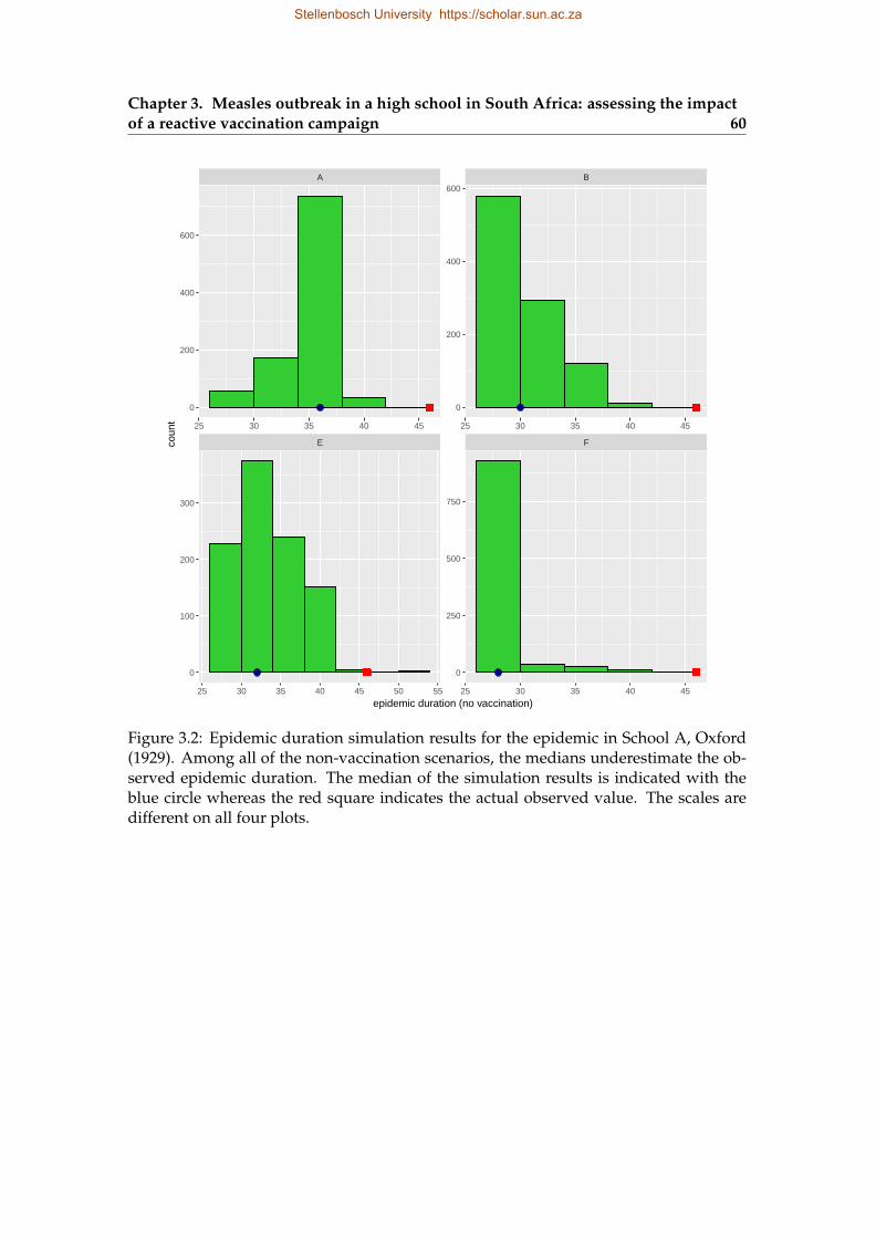
Chapter 3. Measles outbreak in a high school in South Africa: assessing the impactof a reactive vaccination campaign 60
E F
A B
25 30 35 40 45 50 55 25 30 35 40 45
25 30 35 40 45 25 30 35 40 45
0
200
400
600
0
250
500
750
0
200
400
600
0
100
200
300
epidemic duration (no vaccination)
coun
t
Figure 3.2: Epidemic duration simulation results for the epidemic in School A, Oxford(1929). Among all of the non-vaccination scenarios, the medians underestimate the ob-served epidemic duration. The median of the simulation results is indicated with theblue circle whereas the red square indicates the actual observed value. The scales aredifferent on all four plots.
Stellenbosch University https://scholar.sun.ac.za
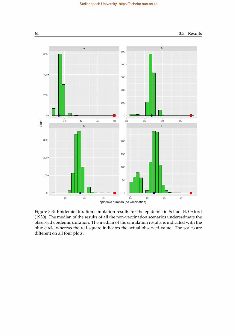
61 3.3. Results
E F
A B
35 40 45 30 35 40 45
39 42 45 48 30 35 40 45
0
100
200
300
400
500
0
50
100
150
200
0
200
400
600
0
100
200
300
epidemic duration (no vaccination)
coun
t
Figure 3.3: Epidemic duration simulation results for the epidemic in School B, Oxford(1930). The median of the results of all the non-vaccination scenarios underestimate theobserved epidemic duration. The median of the simulation results is indicated with theblue circle whereas the red square indicates the actual observed value. The scales aredifferent on all four plots.
Stellenbosch University https://scholar.sun.ac.za
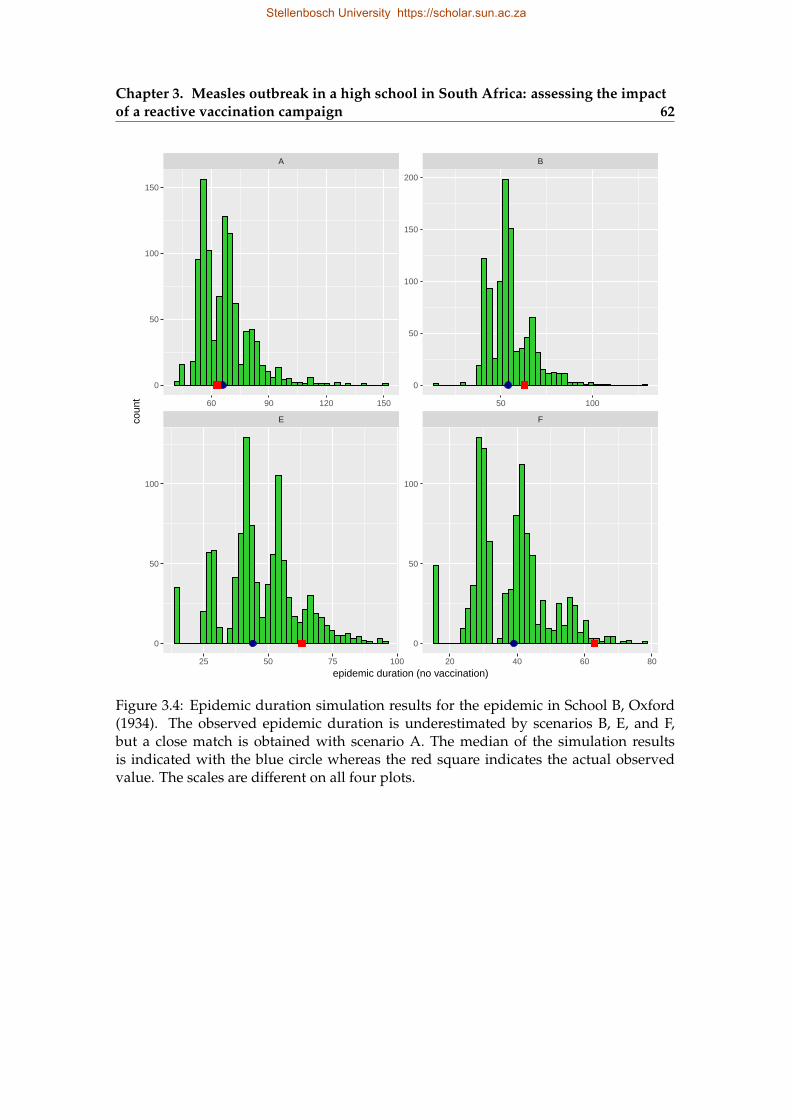
Chapter 3. Measles outbreak in a high school in South Africa: assessing the impactof a reactive vaccination campaign 62
E F
A B
25 50 75 100 20 40 60 80
60 90 120 150 50 100
0
50
100
150
200
0
50
100
0
50
100
150
0
50
100
epidemic duration (no vaccination)
coun
t
Figure 3.4: Epidemic duration simulation results for the epidemic in School B, Oxford(1934). The observed epidemic duration is underestimated by scenarios B, E, and F,but a close match is obtained with scenario A. The median of the simulation resultsis indicated with the blue circle whereas the red square indicates the actual observedvalue. The scales are different on all four plots.
Stellenbosch University https://scholar.sun.ac.za
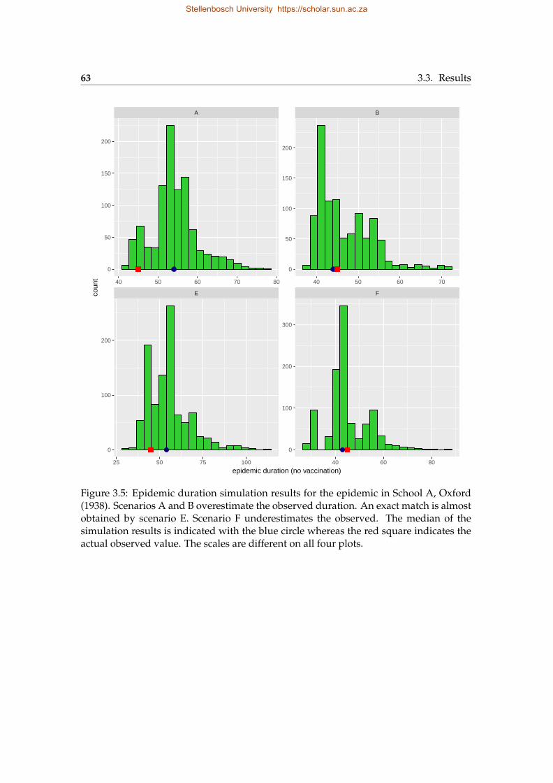
63 3.3. Results
E F
A B
25 50 75 100 40 60 80
40 50 60 70 80 40 50 60 70
0
50
100
150
200
0
100
200
300
0
50
100
150
200
0
100
200
epidemic duration (no vaccination)
coun
t
Figure 3.5: Epidemic duration simulation results for the epidemic in School A, Oxford(1938). Scenarios A and B overestimate the observed duration. An exact match is almostobtained by scenario E. Scenario F underestimates the observed. The median of thesimulation results is indicated with the blue circle whereas the red square indicates theactual observed value. The scales are different on all four plots.
Stellenbosch University https://scholar.sun.ac.za
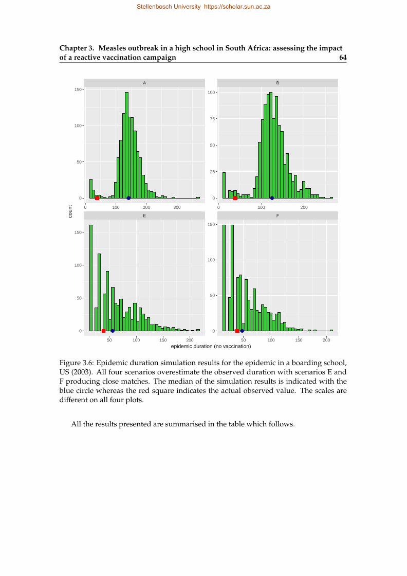
Chapter 3. Measles outbreak in a high school in South Africa: assessing the impactof a reactive vaccination campaign 64
E F
A B
50 100 150 200 50 100 150 200
0 100 200 300 0 100 200
0
25
50
75
100
0
50
100
150
0
50
100
150
0
50
100
150
epidemic duration (no vaccination)
coun
t
Figure 3.6: Epidemic duration simulation results for the epidemic in a boarding school,US (2003). All four scenarios overestimate the observed duration with scenarios E andF producing close matches. The median of the simulation results is indicated with theblue circle whereas the red square indicates the actual observed value. The scales aredifferent on all four plots.
All the results presented are summarised in the table which follows.
Stellenbosch University https://scholar.sun.ac.za
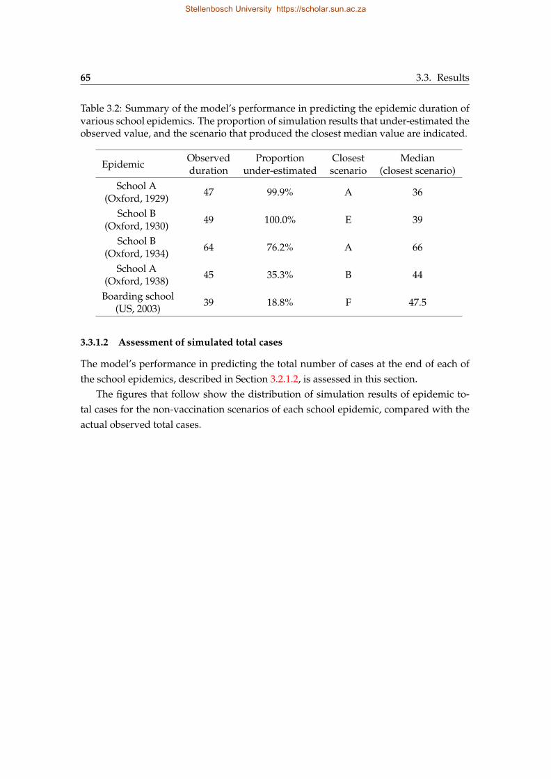
65 3.3. Results
Table 3.2: Summary of the model’s performance in predicting the epidemic duration ofvarious school epidemics. The proportion of simulation results that under-estimated theobserved value, and the scenario that produced the closest median value are indicated.
EpidemicObservedduration
Proportionunder-estimated
Closestscenario
Median(closest scenario)
School A(Oxford, 1929)
47 99.9% A 36
School B(Oxford, 1930)
49 100.0% E 39
School B(Oxford, 1934)
64 76.2% A 66
School A(Oxford, 1938)
45 35.3% B 44
Boarding school(US, 2003)
39 18.8% F 47.5
3.3.1.2 Assessment of simulated total cases
The model’s performance in predicting the total number of cases at the end of each ofthe school epidemics, described in Section 3.2.1.2, is assessed in this section.
The figures that follow show the distribution of simulation results of epidemic to-tal cases for the non-vaccination scenarios of each school epidemic, compared with theactual observed total cases.
Stellenbosch University https://scholar.sun.ac.za
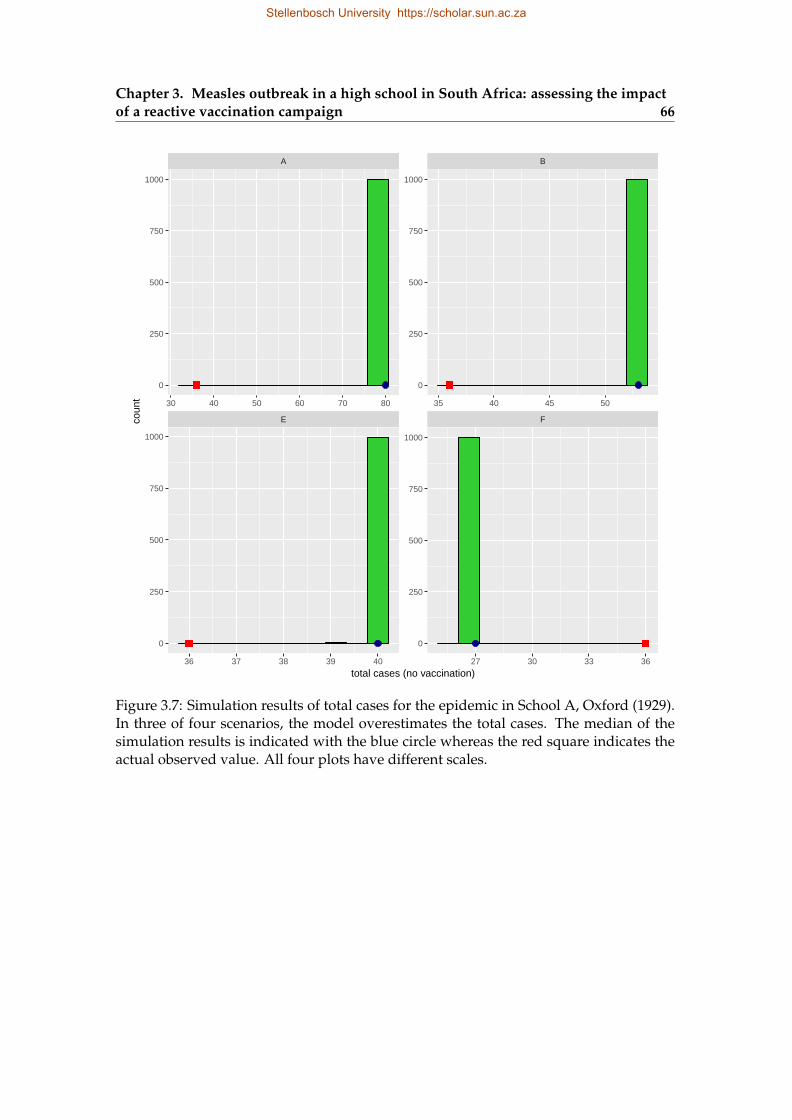
Chapter 3. Measles outbreak in a high school in South Africa: assessing the impactof a reactive vaccination campaign 66
E F
A B
36 37 38 39 40 27 30 33 36
30 40 50 60 70 80 35 40 45 50
0
250
500
750
1000
0
250
500
750
1000
0
250
500
750
1000
0
250
500
750
1000
total cases (no vaccination)
coun
t
Figure 3.7: Simulation results of total cases for the epidemic in School A, Oxford (1929).In three of four scenarios, the model overestimates the total cases. The median of thesimulation results is indicated with the blue circle whereas the red square indicates theactual observed value. All four plots have different scales.
Stellenbosch University https://scholar.sun.ac.za
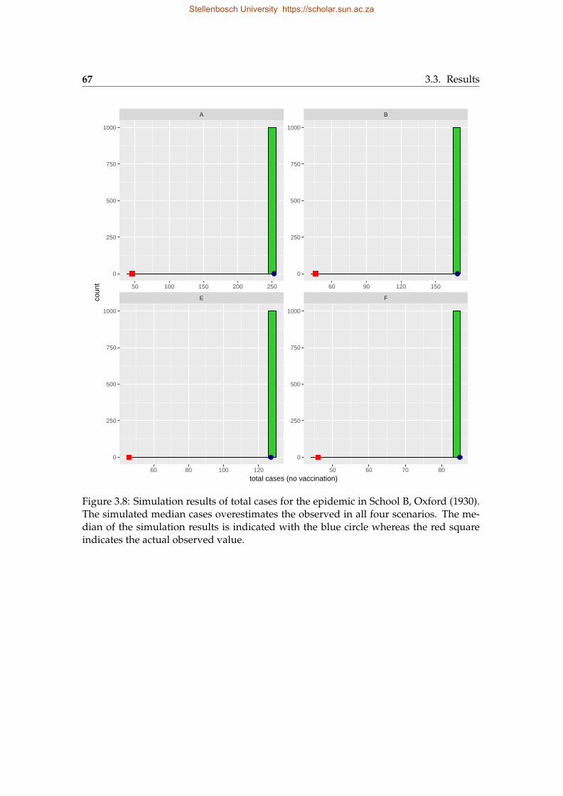
67 3.3. Results
E F
A B
60 80 100 120 50 60 70 80
50 100 150 200 250 60 90 120 150
0
250
500
750
1000
0
250
500
750
1000
0
250
500
750
1000
0
250
500
750
1000
total cases (no vaccination)
coun
t
Figure 3.8: Simulation results of total cases for the epidemic in School B, Oxford (1930).The simulated median cases overestimates the observed in all four scenarios. The me-dian of the simulation results is indicated with the blue circle whereas the red squareindicates the actual observed value.
Stellenbosch University https://scholar.sun.ac.za
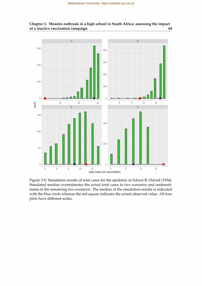
Chapter 3. Measles outbreak in a high school in South Africa: assessing the impactof a reactive vaccination campaign 68
E F
A B
4 6 8 10 12 4 6 8 10
15 20 25 6 9 12 15
0
100
200
300
400
0
100
200
0
100
200
300
0
50
100
150
total cases (no vaccination)
coun
t
Figure 3.9: Simulation results of total cases for the epidemic in School B, Oxford (1934).Simulated median overestimates the actual total cases in two scenarios and underesti-mates in the remaining two scenarios. The median of the simulation results is indicatedwith the blue circle whereas the red square indicates the actual observed value. All fourplots have different scales.
Stellenbosch University https://scholar.sun.ac.za
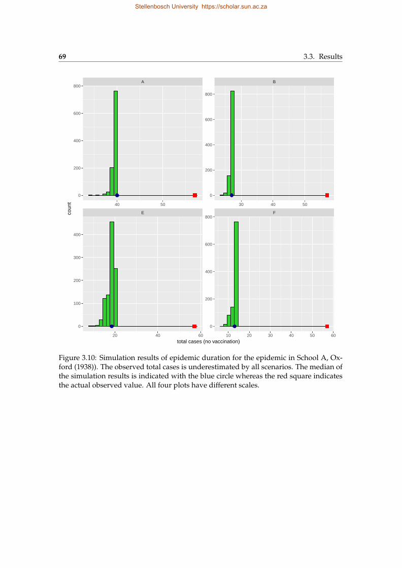
69 3.3. Results
E F
A B
20 40 60 10 20 30 40 50 60
40 50 30 40 50
0
200
400
600
800
0
200
400
600
800
0
200
400
600
800
0
100
200
300
400
total cases (no vaccination)
coun
t
Figure 3.10: Simulation results of epidemic duration for the epidemic in School A, Ox-ford (1938)). The observed total cases is underestimated by all scenarios. The median ofthe simulation results is indicated with the blue circle whereas the red square indicatesthe actual observed value. All four plots have different scales.
Stellenbosch University https://scholar.sun.ac.za
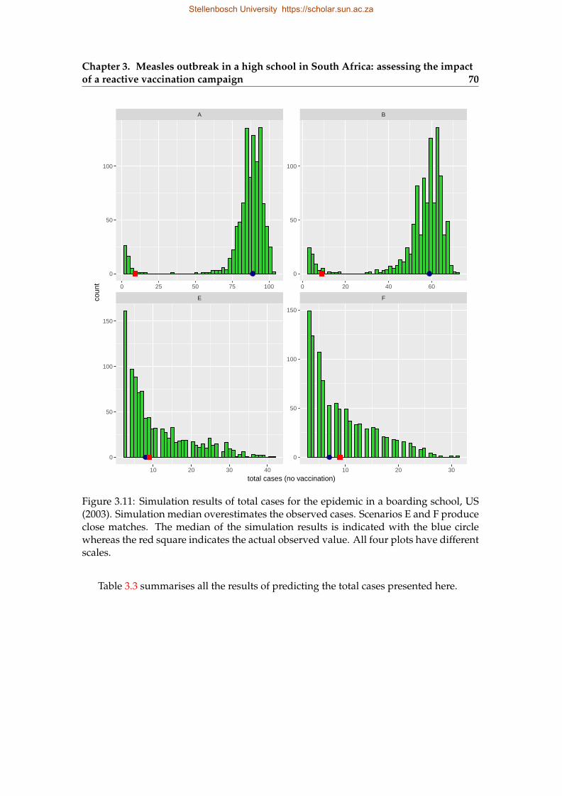
Chapter 3. Measles outbreak in a high school in South Africa: assessing the impactof a reactive vaccination campaign 70
E F
A B
10 20 30 40 10 20 30
0 25 50 75 100 0 20 40 60
0
50
100
0
50
100
150
0
50
100
0
50
100
150
total cases (no vaccination)
coun
t
Figure 3.11: Simulation results of total cases for the epidemic in a boarding school, US(2003). Simulation median overestimates the observed cases. Scenarios E and F produceclose matches. The median of the simulation results is indicated with the blue circlewhereas the red square indicates the actual observed value. All four plots have differentscales.
Table 3.3 summarises all the results of predicting the total cases presented here.
Stellenbosch University https://scholar.sun.ac.za
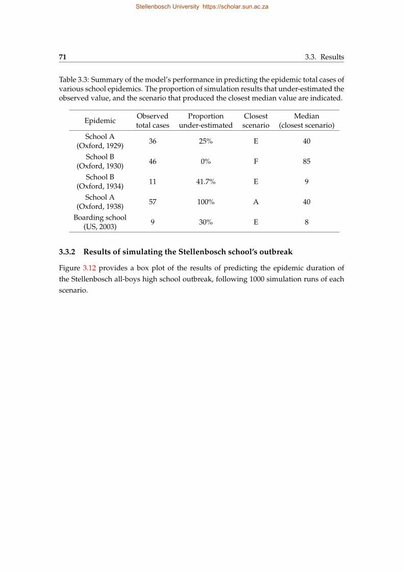
71 3.3. Results
Table 3.3: Summary of the model’s performance in predicting the epidemic total cases ofvarious school epidemics. The proportion of simulation results that under-estimated theobserved value, and the scenario that produced the closest median value are indicated.
EpidemicObservedtotal cases
Proportionunder-estimated
Closestscenario
Median(closest scenario)
School A(Oxford, 1929)
36 25% E 40
School B(Oxford, 1930)
46 0% F 85
School B(Oxford, 1934)
11 41.7% E 9
School A(Oxford, 1938)
57 100% A 40
Boarding school(US, 2003)
9 30% E 8
3.3.2 Results of simulating the Stellenbosch school’s outbreak
Figure 3.12 provides a box plot of the results of predicting the epidemic duration ofthe Stellenbosch all-boys high school outbreak, following 1000 simulation runs of eachscenario.
Stellenbosch University https://scholar.sun.ac.za
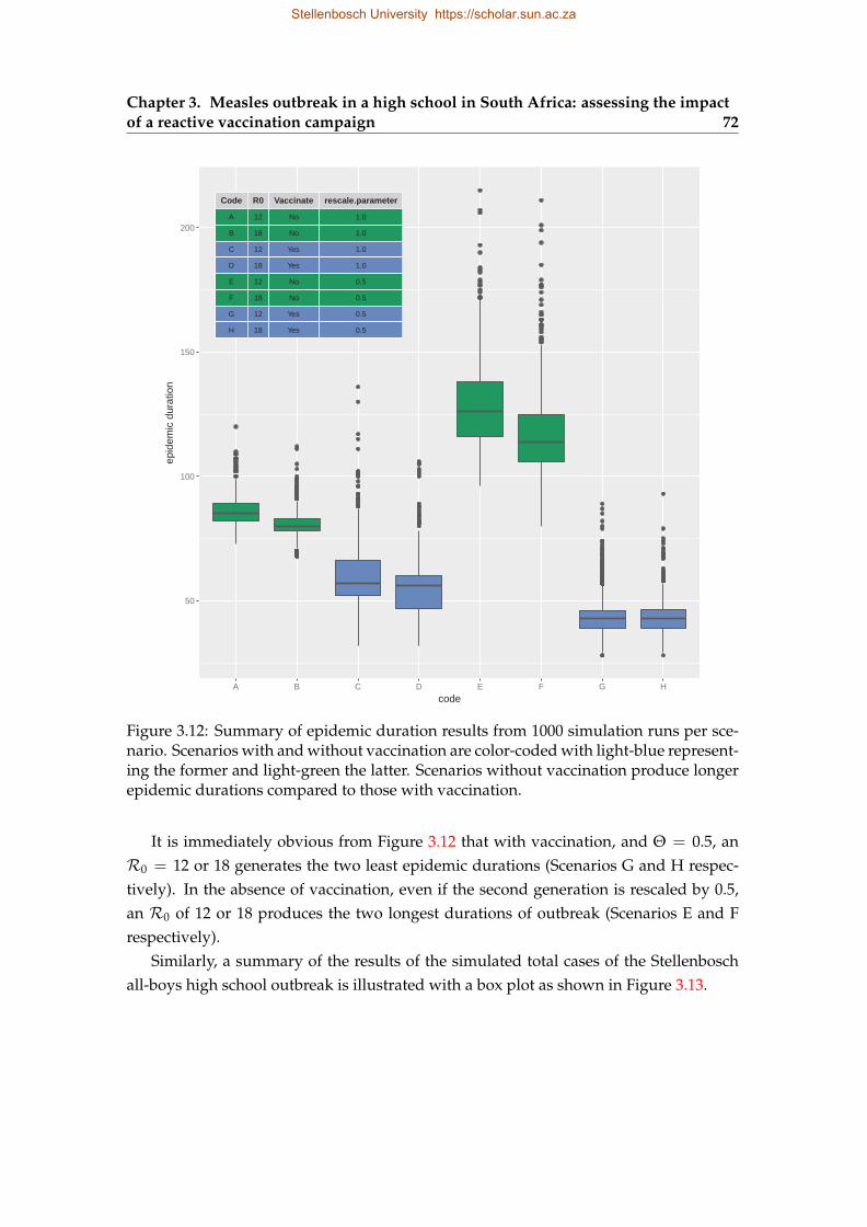
Chapter 3. Measles outbreak in a high school in South Africa: assessing the impactof a reactive vaccination campaign 72
Code
A
R0
B
Vaccinate
C
rescale.parameter
D
E
F
G
H
12
18
12
18
12
18
12
18
No
No
Yes
Yes
No
No
Yes
Yes
1.0
1.0
1.0
1.0
0.5
0.5
0.5
0.5
50
100
150
200
A B C D E F G H
code
epid
emic
dur
atio
n
Figure 3.12: Summary of epidemic duration results from 1000 simulation runs per sce-nario. Scenarios with and without vaccination are color-coded with light-blue represent-ing the former and light-green the latter. Scenarios without vaccination produce longerepidemic durations compared to those with vaccination.
It is immediately obvious from Figure 3.12 that with vaccination, and Θ = 0.5, anR0 = 12 or 18 generates the two least epidemic durations (Scenarios G and H respec-tively). In the absence of vaccination, even if the second generation is rescaled by 0.5,an R0 of 12 or 18 produces the two longest durations of outbreak (Scenarios E and Frespectively).
Similarly, a summary of the results of the simulated total cases of the Stellenboschall-boys high school outbreak is illustrated with a box plot as shown in Figure 3.13.
Stellenbosch University https://scholar.sun.ac.za
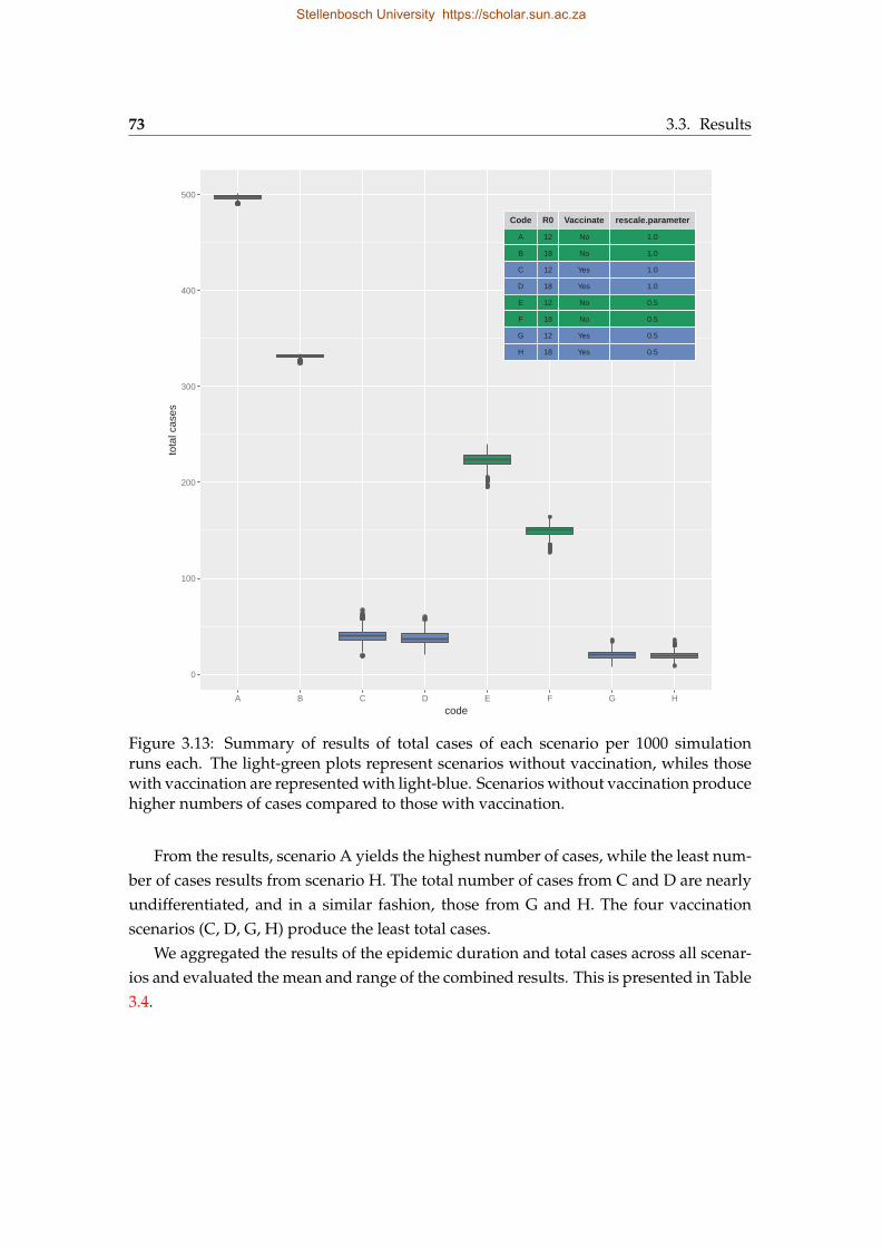
73 3.3. Results
Code
A
R0
B
Vaccinate
C
rescale.parameter
D
E
F
G
H
12
18
12
18
12
18
12
18
No
No
Yes
Yes
No
No
Yes
Yes
1.0
1.0
1.0
1.0
0.5
0.5
0.5
0.5
0
100
200
300
400
500
A B C D E F G H
code
tota
l cas
es
Figure 3.13: Summary of results of total cases of each scenario per 1000 simulationruns each. The light-green plots represent scenarios without vaccination, whiles thosewith vaccination are represented with light-blue. Scenarios without vaccination producehigher numbers of cases compared to those with vaccination.
From the results, scenario A yields the highest number of cases, while the least num-ber of cases results from scenario H. The total number of cases from C and D are nearlyundifferentiated, and in a similar fashion, those from G and H. The four vaccinationscenarios (C, D, G, H) produce the least total cases.
We aggregated the results of the epidemic duration and total cases across all scenar-ios and evaluated the mean and range of the combined results. This is presented in Table3.4.
Stellenbosch University https://scholar.sun.ac.za
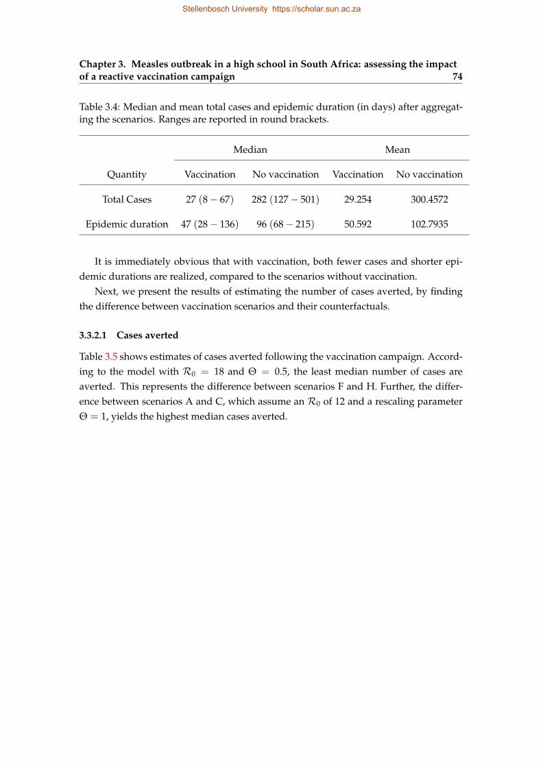
Chapter 3. Measles outbreak in a high school in South Africa: assessing the impactof a reactive vaccination campaign 74
Table 3.4: Median and mean total cases and epidemic duration (in days) after aggregat-ing the scenarios. Ranges are reported in round brackets.
Median Mean
Quantity Vaccination No vaccination Vaccination No vaccination
Total Cases 27 (8− 67) 282 (127− 501) 29.254 300.4572
Epidemic duration 47 (28− 136) 96 (68− 215) 50.592 102.7935
It is immediately obvious that with vaccination, both fewer cases and shorter epi-demic durations are realized, compared to the scenarios without vaccination.
Next, we present the results of estimating the number of cases averted, by findingthe difference between vaccination scenarios and their counterfactuals.
3.3.2.1 Cases averted
Table 3.5 shows estimates of cases averted following the vaccination campaign. Accord-ing to the model with R0 = 18 and Θ = 0.5, the least median number of cases areaverted. This represents the difference between scenarios F and H. Further, the differ-ence between scenarios A and C, which assume an R0 of 12 and a rescaling parameterΘ = 1, yields the highest median cases averted.
Stellenbosch University https://scholar.sun.ac.za
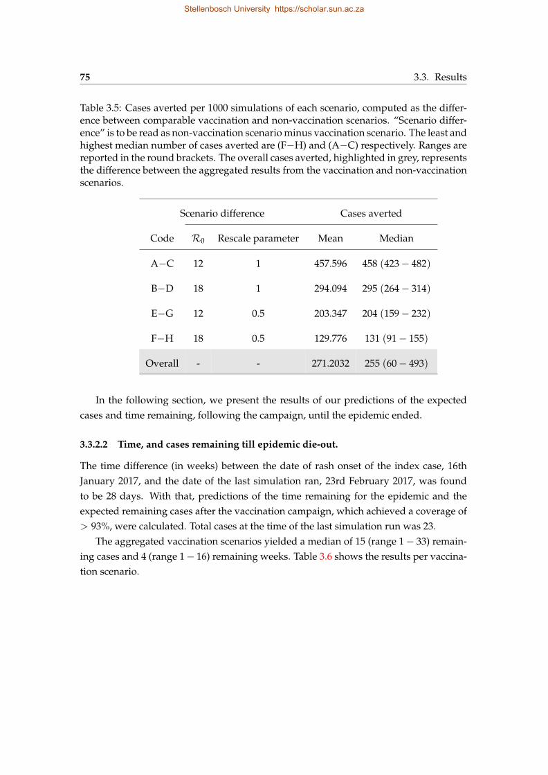
75 3.3. Results
Table 3.5: Cases averted per 1000 simulations of each scenario, computed as the differ-ence between comparable vaccination and non-vaccination scenarios. “Scenario differ-ence” is to be read as non-vaccination scenario minus vaccination scenario. The least andhighest median number of cases averted are (F−H) and (A−C) respectively. Ranges arereported in the round brackets. The overall cases averted, highlighted in grey, representsthe difference between the aggregated results from the vaccination and non-vaccinationscenarios.
Scenario difference Cases averted
Code R0 Rescale parameter Mean Median
A−C 12 1 457.596 458 (423− 482)
B−D 18 1 294.094 295 (264− 314)
E−G 12 0.5 203.347 204 (159− 232)
F−H 18 0.5 129.776 131 (91− 155)
Overall - - 271.2032 255 (60− 493)
In the following section, we present the results of our predictions of the expectedcases and time remaining, following the campaign, until the epidemic ended.
3.3.2.2 Time, and cases remaining till epidemic die-out.
The time difference (in weeks) between the date of rash onset of the index case, 16thJanuary 2017, and the date of the last simulation ran, 23rd February 2017, was foundto be 28 days. With that, predictions of the time remaining for the epidemic and theexpected remaining cases after the vaccination campaign, which achieved a coverage of> 93%, were calculated. Total cases at the time of the last simulation run was 23.
The aggregated vaccination scenarios yielded a median of 15 (range 1− 33) remain-ing cases and 4 (range 1− 16) remaining weeks. Table 3.6 shows the results per vaccina-tion scenario.
Stellenbosch University https://scholar.sun.ac.za
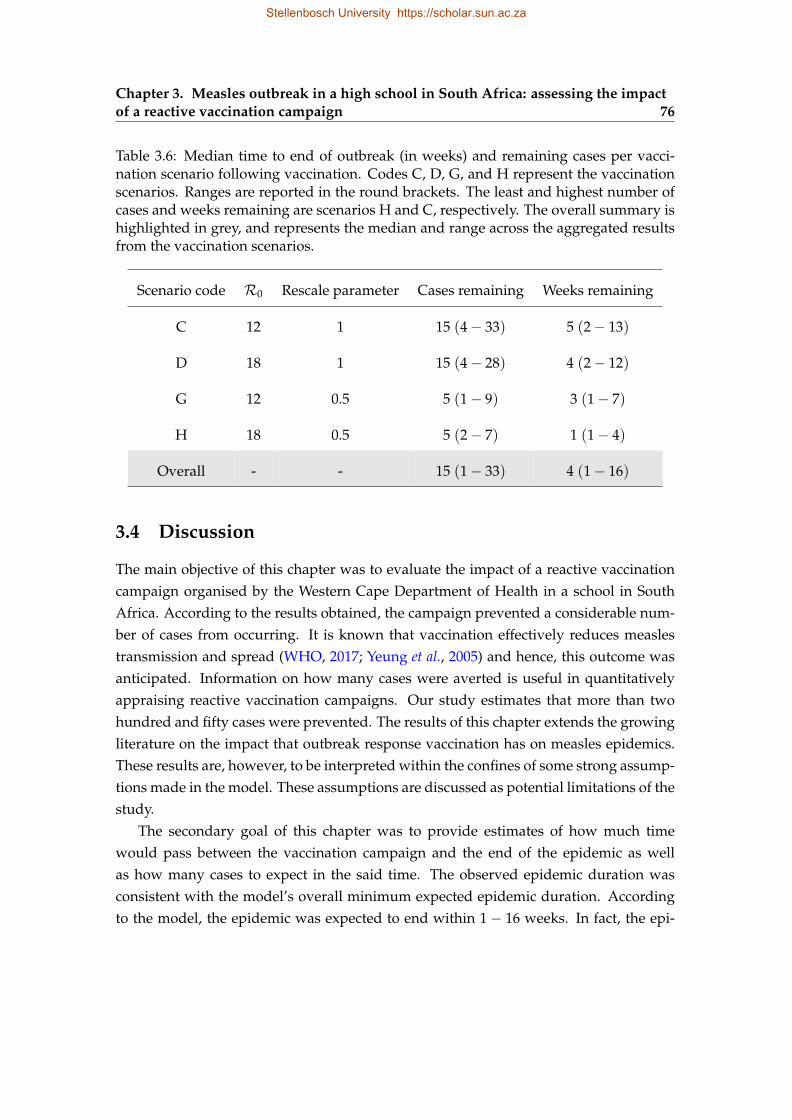
Chapter 3. Measles outbreak in a high school in South Africa: assessing the impactof a reactive vaccination campaign 76
Table 3.6: Median time to end of outbreak (in weeks) and remaining cases per vacci-nation scenario following vaccination. Codes C, D, G, and H represent the vaccinationscenarios. Ranges are reported in the round brackets. The least and highest number ofcases and weeks remaining are scenarios H and C, respectively. The overall summary ishighlighted in grey, and represents the median and range across the aggregated resultsfrom the vaccination scenarios.
Scenario code R0 Rescale parameter Cases remaining Weeks remaining
C 12 1 15 (4− 33) 5 (2− 13)
D 18 1 15 (4− 28) 4 (2− 12)
G 12 0.5 5 (1− 9) 3 (1− 7)
H 18 0.5 5 (2− 7) 1 (1− 4)
Overall - - 15 (1− 33) 4 (1− 16)
3.4 Discussion
The main objective of this chapter was to evaluate the impact of a reactive vaccinationcampaign organised by the Western Cape Department of Health in a school in SouthAfrica. According to the results obtained, the campaign prevented a considerable num-ber of cases from occurring. It is known that vaccination effectively reduces measlestransmission and spread (WHO, 2017; Yeung et al., 2005) and hence, this outcome wasanticipated. Information on how many cases were averted is useful in quantitativelyappraising reactive vaccination campaigns. Our study estimates that more than twohundred and fifty cases were prevented. The results of this chapter extends the growingliterature on the impact that outbreak response vaccination has on measles epidemics.These results are, however, to be interpreted within the confines of some strong assump-tions made in the model. These assumptions are discussed as potential limitations of thestudy.
The secondary goal of this chapter was to provide estimates of how much timewould pass between the vaccination campaign and the end of the epidemic as wellas how many cases to expect in the said time. The observed epidemic duration wasconsistent with the model’s overall minimum expected epidemic duration. Accordingto the model, the epidemic was expected to end within 1− 16 weeks. In fact, the epi-
Stellenbosch University https://scholar.sun.ac.za
77 3.4. Discussion
demic had actually ended by the time we were running our analyses, a few weeks afterthe campaign. The model also predicted a range of 1− 33 remaining cases. The modelonly focused on the number of cases among learners in the school, and we do not knowhow many of the cases post-vaccination actually occurred in this population, but we arecertain the observed remaining cases was captured within the predicted bounds of themodel.
The results of the secondary goal would have been important for planning ahead.Even though the results were useful for communication, they were not timely enoughto be useful as a real-time tool for assessment and decision-making. Nevertheless, themethods we employed to achieve the results can be improved for studying closed-population measles epidemics in real-time. For modelling outcomes in fast outbreaksettings like that of measles it is preferable that the model be ready sometime in ad-vance to facilitate real-time predictions and communications.
Measles outbreak response strategies dictate that the highest possible vaccinationcoverage attainable is prioritized over every other outcome, but studies have shown thatin some cases, speed of response is more important (Ferrari et al., 2014; Grais et al., 2007).In this light, the reactive campaign organized in the high school was fast relative to theepidemic progression and achieved a high coverage (≈ 93%). The estimate of casesaverted obtained from this study is, therefore, testament to the importance of responsespeed and high vaccination coverage. This study did not, however, explicitly study howthe timing of the intervention influenced the results.
The mere occurrence of the outbreak in the school after a several years of no out-breaks deserves further investigation. It is clearly an indication of the possible existenceof a pool of susceptible learners, built up over time. Even though there were only 5 con-firmed cases at the time of the campaign, the 23 cases that followed marked its climaxand points to the existence of high susceptibility in the population. A susceptible poolbuilds up due to non-uptake of the vaccine, often for religious reasons; immunizationfailure among some of the learners; loss of immunity; and lack of previous exposure tothe infection (WHO, 2017). This outbreak warrants the need to investigate immunitylevels among learners, not only in the affected school but in the whole province. Vacci-nation uptake should be encouraged to ensure sero-conversion among the learners whomay have failed previous vaccination attempts. This is so that the herd immunity ofmeasles is achieved to protect against future outbreaks. If measles elimination is a goalin the province, this is an important next step.
Stellenbosch University https://scholar.sun.ac.za
Chapter 3. Measles outbreak in a high school in South Africa: assessing the impactof a reactive vaccination campaign 78
3.4.1 Potential limitations
We assumed the range of widely citedR0 values of 12 and 18 in formulating the multiplescenarios. It is known that R0 varies widely and is context-specific (Guerra et al., 2017).Future extensions of this study will include a broader range ofR0 values to compensatefor the uncertainties surrounding the actual value.
Another potential limitation of our modelling approach was the assumption that thevaccine had 100% efficacy and that the immune response was instantaneous, therebyneglecting the time delay until an immune response kicks in. The former assumptionis contrary to other modelling studies in developing countries which assume lower effi-cacy rates (Grais et al., 2007; Lessler et al., 2016). However, considering South Africa is ahybrid of developing and developed provinces, with the Western Cape province beingdeveloped and highly-resourced in the health sector, we made vaccine efficacy assump-tions relevant to high-resource settings. This assumption followed after we had carefullyexamined the reasons behind loss of efficacy in measles vaccines, and compared themwith the characteristics of the population we were modelling, and the current state ofaffairs at the Western Cape Department of Health. This assumption is realistic as somemeasles vaccine efficacy studies in developed countries have estimated this quantity tobe 100% or close to it (Uzicanin & Zimmerman, 2011). Vaccines remain efficacious whenthey are stored in subzero temperatures until they are administered. Also, the young ageof vaccinees, associated with the possession of passively acquired maternal antibodiesmentioned in Chapter 1 is another hindrance to efficacy (Aaby et al., 1990). These criteriawere not applicable to our study since the individuals in consideration were predomi-nantly teenagers. Also, since the Department of Health in the Western Cape province iswell-funded, it was our reasoning that the cold chain is well-managed to ensure the vac-cines are stable and efficacious. We, therefore, consider it unlikely that the assumptionabout vaccine efficacy substantially biased our estimates. The assumption regarding thetiming of the immune response, however, is a strong assumption with the potential toinfluence the results. Hence, the results obtained here are to be interpreted with caution.Future studies will investigate the effect of this delay.
The model did not fare too well in predicting the dynamics of other school epidemicsduring our validation. This may be due to a mismatch between the actual reproductionnumbers (Re f f and R0) in those epidemics, compared with what was assumed in themodel scenarios, or differences in other parameters. We intend to revise our assump-tions and perform further assessments to ensure our predictions are more realistic foruse in future outbreak situations. As a consequence of this limitation, we report ourestimates with some level of caution. The approach we employed can be refined and
Stellenbosch University https://scholar.sun.ac.za
79 3.4. Discussion
made more rigorous by relaxing some of our assumptions to improve the model’s per-formance.
Additionally, a major constraint when modelling outcomes during outbreaks is timeand uncertainty in decision-making and this was no different in our case. As a result,some of the decisions taken during the modelling process may have been made hastily.A choice needed to be made between making speedy and simplistic assumptions toaccount for uncertainties, or being more thoughtful but taking a longer time to respondto the outbreak. We chose the former. We, however, tried to keep the uncertainties undercheck by making assumptions specific to this particular outbreak.
3.4.2 Information brokerage
A secondary goal of outbreak response, according to the WHO guidelines is communityawareness as prevention (WHO, 2009). In order to help achieve this goal at the time,several strategies were utilized. We will now proceed to discuss them.
3.4.2.1 Measles information sheets
Two kinds of information sheets were designed and distributed. The first, found inAppendix A.1, was distributed to the general public both electronically and on no-tice boards across the Stellenbosch university campus, as well as the surrounding highschools. The sheet contained information about the natural history of the disease aswell as its means of spread. It also explained the advantages of being vaccinated againstmeasles and gave instructions on what should be done in case an individual was foundshowing suspicious symptoms. We included information on the various clinics andpharmacies offering vaccination and case management services in Stellenbosch and itsenvirons. Each of these clinics and pharmacies were contacted to ascertain the servicesthey provided and associated costs. Pertaining to the costs, even though the govern-ment facilities provided free services, the private ones offered them at variable costs.All this information was translated into two of the most widely spoken languages in theWestern Cape province: Afrikaans (translated by a SACEMA associate) and isiXhosa(translated by the Stellenbosch University Language Center).
The other sheet, included in Appendix A.2, was specific to the affected high school.It contained information on how many cases had been prevented, and how the epidemicwas expected to progress in terms of the cases and time to expect until the epidemic hadsubsided following the vaccination campaign.
Stellenbosch University https://scholar.sun.ac.za
Chapter 3. Measles outbreak in a high school in South Africa: assessing the impactof a reactive vaccination campaign 80
All school principals in the vicinity of the affected school were emailed with copiesof the sheets in Appendix A.1 for further proliferation. The latter sheet, A.2, was sent tothe principal of the affected high school under study and forwarded to the school com-munity. The school recognized our efforts and this was acknowledged on their website.The following link directs you to the acknowledgment: https://www.paulroos.co.za/masels-measles/.
3.4.2.2 Web application for learners
We developed a web application using the R statistical language’s (R Core Team, 2017)RShiny package version 1.0.5 (Chang et al., 2017). The application was deployed to theschool and neighbouring schools, after it was hosted on a landing web page. The ap-plication was designed to give the school’s staff and learners insights into how the fieldof epidemiological modelling is employed to control the spread of infections. It wasour hope that the application would boost mathematics pedagogy in the school as wellas the learners’ interests in the subject of mathematics. We also hoped to introduce thelearners to epidemiological modelling as one of the many specializations in mathemati-cal science.
The application consists of various tabs for learning about this specific measles out-break including a tab under which the user can tweak certain parameters which de-termine the size and duration of the outbreak including: number of learners in theschool (N), number of learners infected by the index case Re f f , timing of the outbreak re-sponse vaccination after diagnosis of the first case with a rash, and vaccination coverageachieved through the campaign. Another tab shows what could have happened withoutthe vaccination in the best and worst case scenarios. The final tab explains a variety ofconcepts including: the plots displayed in the other tabs as well as the terminology used,and how the calculations were done in non-technical terms. This tab also describes someother applications of epidemiological modelling and how some other SACEMA (SouthAfrican Center of Excellence for Epidemiological Modelling and Analysis)-affiliated re-searchers have successfully used mathematical modelling tools in disease managementand control across the world.
The following is a link for accessing the application: http://measles.sacema.org/.Additionally, the implementation code for this chapter is hosted on a private githubrepository, available upon the reader’s request.
Stellenbosch University https://scholar.sun.ac.za
Chapter 4
Conclusion
This thesis has answered two main questions, with an overarching aim of contributingto what is known about the two measles parameter estimation methods, and outbreakresponse vaccination impact assessment.
We started off in Chapter 1 by engaging with the ongoing scholarly conversationabout measles dynamical modelling, methods for parametrizing measles models, andthe impact of outbreak response vaccination. In Chapter 2, “Evaluating two methodsfor estimating measles parameters”, we demonstrated that the performance of two well-known methods of fitting measles data, namely, the time series susceptible-infected-recovered model (Bjørnstad et al., 2002) and the removal method (Ferrari et al., 2005),depends on the assumptions underlying the data generation process, degree of spatialaggregation of the cases, the artificial methods employed to put the data in a form usablefor each of the two models, and the parameter being fitted. In Chapter 3, “Measlesoutbreak in a high school in South Africa: assessing the impact of a reactive vaccinationcampaign”, we assessed the impact of a reactive campaign organized by the WesternCape province’s Department of Health in response to an outbreak in an all-boys highschool in the town of Stellenbosch in South Africa. We found the reactive campaign tohave been successful in preventing hundreds of cases and reducing the duration of theepidemic.
In-depth discussions of our findings have already been provided in each of the ear-lier chapters. Here, we suggest some implications of the findings of this thesis on twomain aspects of the existing literature, namely, measles model parameterization, andoutbreak response vaccination.
81
Stellenbosch University https://scholar.sun.ac.za
Chapter 4. Conclusion 82
4.1 Implications of findings on measles modelparameterization
Measles data fitting techniques, like the two we evaluated in Chapter 2, are usually for-mulated for well-curated, high quality data sets. Such data sets are not readily availablein developing countries. When the data being fitted does not conform to that requiredby these types of models, decisions have to be made in the data modification process.Biases resulting from these modifications and the fitting process should be documentedto guide how the estimates are interpreted.
The results of Chapter 2 imply that when parameters are fitted from large degrees ofspatially aggregated data, the estimates are biased and hence the model’s performancediminishes. Therefore, the results of estimates at this level of aggregation should beinterpreted with caution.
The removal method tends to estimate S0 with less bias, even when each 0 in thecase time series is replaced with 1, but exaggerates Re f f in non-naive populations. TheR0 estimates from the naive populations are biased but at a lower order of magnitudecompared with those from the non-naive populations. The biases in the Re f f estimatesare, therefore, driven by the fact that the population is non-naive and, therefore, violatesthe removal method’s assumption of naiveness. This indicates that it is not advisableto fit non-naive populations with the removal method. When applying the removalmethod to data interspersed with zero cases, care should be taken in interpreting Re f f
andR0, especially after the zero cases have been replaced with alternatives.In future assessments, other approaches of dealing with zero cases should be tested,
and the biases compared, in order to determine the approaches that produce unbiasedestimates.
4.2 Implications of findings on outbreak response vaccination
The work done in Chapter 3 provides, at the least, a simple model for assessing outbreakresponse vaccination in closed populations. The limitations of the model have alreadybeen addressed in Section 3.4, including, most importantly, the assumption about vac-cine efficacy, as it has to be as context-specific as possible in our case.
As epidemic data becomes available, the model should be parameterized and read-ied for future outbreaks as elimination is being targeted. We mentioned in our discus-sions in Section 3.4 that time was a constraint in our modelling response to the outbreak.It is therefore important that models should be developed in advance, in anticipation of
Stellenbosch University https://scholar.sun.ac.za
83 4.2. Implications of findings on outbreak response vaccination
future outbreaks.The outbreak response strategy mounted by the Department of Health was a success,
since it averted a median of over 250 cases, in the confines of our modelling assumptions.Even though we did not explicitly investigate how the speed of the response affectedthe outcome, it is likely that the response time, coupled with the vaccination coverageachieved, were the reasons for the short epidemic. There are valuable lessons in thisstrategy for international efforts at achieving measles elimination, that is, to improve re-sponse time during outbreaks in closed populations - aggregation of school-going chil-dren drives measles epidemics, and if response is delayed, school epidemics can serveas hot beds for national outbreaks, thereby marring efforts at achieving local measleselimination.
Finally, it is known that in countries where vaccination has been well implemented,there is a shift in the mean age of infection from below 5 years to the teens. The outbreakin Stellenbosch provides clear evidence of the need to boost surveillance and immunityof school-going children to reduce the rate of build-up of susceptible pools. Healthbudgets should include measles serological surveys to help bridge the immunity gapsto facilitate achieving the measles elimination goal.
Stellenbosch University https://scholar.sun.ac.za

Appendices
84
Stellenbosch University https://scholar.sun.ac.za
Appendix A
Here, we present the information sheets described in the summary section of Chapter 3.
A.1 Information Sheets in English, Afrikaans, and isiXhosa
85
Stellenbosch University https://scholar.sun.ac.za
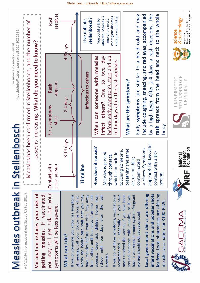
Co
nta
ct w
ith
a
sick
per
son
Ea
rly
sym
pto
ms
star
t R
ash
ap
pea
rs
Ras
h
reso
lves
Wh
at a
re t
he
sym
pto
ms?
Ea
rly
sym
pto
ms
are
sim
ilar
to a
he
ad c
old
an
d m
ay
incl
ud
e c
ou
ghin
g, s
nee
zin
g, a
nd
red
eye
s, a
cco
mp
anie
d
by
a h
igh
fev
er.
Aft
er 2
-4 d
ays,
a r
ash
dev
elo
ps.
Th
e
rash
sp
read
s fr
om
th
e h
ead
an
d n
eck
to t
he
wh
ole
b
od
y.
Ho
w d
oe
s it
sp
read
? M
easl
es is
pas
sed
th
rou
gh c
on
tact
, w
hic
h c
an in
clu
de
tou
chin
g so
meo
ne,
b
reat
hin
g th
e sa
me
air,
or
tou
chin
g co
nta
min
ated
su
rfac
es. S
ymp
tom
s ap
pea
r 8
-14
day
s af
ter
con
tact
wit
h a
sic
k p
erso
n.
8-1
4 d
ays
2-4
day
s
Tim
elin
e
Wh
en
ca
n s
om
eo
ne
wit
h m
eas
les
infe
ct
oth
ers
? O
ne
to
two
d
ay
bef
ore
ear
ly s
ymp
tom
s st
art
and
up
to
fo
ur
day
s af
ter
the
rash
ap
pea
rs.
Infe
ctio
us
to o
the
rs
4-8
day
s W
hat
can
I d
o?
Loca
l go
vern
men
t cl
inic
s ar
e o
ffer
ing
infa
nt
vacc
inat
ion
s an
d b
oo
ste
r sh
ots
fo
r fr
ee
. Lo
cal p
har
mac
ies
are
off
erin
g m
easl
es v
acci
nat
ion
fo
r R
10
0-R
22
0.
Vac
cin
atio
n r
ed
uce
s yo
ur
risk
of
gett
ing
me
asle
s.
If
vacc
inat
ed,
you
m
ay
still
ge
t si
ck,
bu
t yo
ur
sym
pto
ms
will
be
less
sev
ere.
If y
ou
or
som
eon
e y
ou
kn
ow
has
sym
pto
ms
of
mea
sles
, ca
ll yo
ur
do
cto
r o
r lo
cal
clin
ic.
No
tify
th
e h
ealt
h c
are
staf
f th
at y
ou
may
h
ave
mea
sles
bef
ore
yo
ur
visi
t. S
tay
away
fr
om
oth
ers
un
til
fou
r d
ays
afte
r th
e r
ash
ap
pea
rs.
Keep
si
ck
child
ren
h
om
e
fro
m
sch
oo
l u
nti
l fo
ur
day
s af
ter
the
ra
sh
app
ears
. If
yo
u d
o n
ot
hav
e s
ymp
tom
s, v
acci
nat
ion
is
reco
mm
en
ded
–
es
pec
ially
if
yo
u
hav
e n
ever
rec
eive
d t
he
vac
cin
e, if
yo
u h
ave
bee
n
aro
un
d
som
eon
e
wit
h m
easl
es,
or
if
you
h
ave
a w
eake
ned
imm
un
e s
yste
m.
Pre
gnan
t w
om
en s
ho
uld
no
t ge
t va
ccin
ated
.
A S
AC
EMA
Info
rmat
ion
Sh
eet
(Iss
ued
08
Feb
20
17
)
Live
ou
tsid
e
Ste
llen
bo
sch
?
You
co
uld
sti
ll b
e af
fect
ed
. Mea
sles
is
on
e o
f th
e m
ost
co
nta
gio
us
dis
ease
s an
d s
pre
ads
qu
ickl
y!
Mea
sles
ou
tbre
ak in
Ste
llen
bo
sch
M
easl
es h
as b
een
co
nfi
rmed
in S
telle
nb
osc
h, a
nd
th
e n
um
be
r o
f ca
ses
is in
crea
sin
g. W
hat
do
yo
u n
ee
d t
o k
no
w?
For
mo
re in
form
atio
n, e
mai
l m
eas
lesi
nfo
@sa
cem
a.o
rg o
r ca
ll 0
21
80
8 2
58
9.
Stellenbosch University https://scholar.sun.ac.za

A S
AC
EMA
Info
rmat
ion
Sh
eet
(Iss
ued
08
Feb
20
17
)
Mea
sles
ou
tbre
ak in
Ste
llen
bo
sch
Fo
r m
ore
info
rmat
ion
, em
ail
me
asle
sin
fo@
sace
ma.
org
or
call
02
1 8
08
25
89
.
Loca
l go
vern
me
nt
clin
ics
are
off
erin
g in
fan
t va
ccin
atio
ns
and
bo
ost
er s
ho
ts f
or
free
. Fi
nd
a c
linic
ne
ar y
ou
.
Clo
ete
svill
e C
om
mu
nit
y H
eal
th C
linic
Te
nn
antv
ille
Stre
et, S
telle
nb
osc
h
02
1 8
83
26
76
Fr
ansc
hh
oe
k Sa
telli
te C
linic
A
kad
emie
Str
eet
Fran
sch
ho
ek
02
1 8
76
21
72
G
roe
nd
al K
linie
k 1
Sti
ebeu
elst
r, F
ran
sch
ho
ek
02
1 8
76
37
14
Id
as V
alle
y C
linic
H
amm
and
shan
d W
ay Id
as V
alle
y, S
telle
nb
osc
h
02
1 8
87
27
21
Jam
est
ow
n C
linic
Pa
jero
Str
eet,
Jam
esto
wn
, Ste
llen
bo
sch
0
21
88
0 0
35
7
K
ayam
and
i Clin
ic
56
Bas
si S
tree
t, K
ayam
and
i, St
elle
nb
osc
h
02
1 8
89
50
61
K
yle
mo
re C
linic
1
9 S
cho
ol S
tree
t, K
ylem
ore
0
21
88
5 2
50
4
R
ho
de
s Fr
uit
Far
m C
linic
G
roo
t D
rake
nst
ein
, 76
80
0
21
87
4 1
11
2
Som
ers
et W
est
Clin
ic
28
Ch
urc
h S
tree
t, S
om
erse
t W
est
02
1 4
44
44
52
V
icto
ria
Stre
et C
linic
5
Vic
tori
a St
reet
, Ste
llen
bo
sch
0
21
88
7 2
65
0
Peo
ple
wit
h w
eak
imm
un
e sy
stem
s -
incl
ud
ing
bab
ies
and
p
eop
le
livin
g w
ith
HIV
- h
ave
the
hig
hes
t ri
sk o
f co
mp
licat
ion
s as
soci
ated
w
ith
m
easl
es
infe
ctio
n.
Vac
cin
atio
n
is
stro
ngl
y re
com
men
ded
fo
r th
ese
in
div
idu
als.
Pre
gnan
t w
om
en s
ho
uld
n
ot
get
vacc
inat
ed.
Stellenbosch University https://scholar.sun.ac.za

Ko
nta
k m
et ‘n
si
ek p
erso
on
V
roeë
sim
pto
me
b
egin
U
itsl
ag
beg
in
Uit
slag
ve
rdw
yn
Wat
is d
ie s
imp
tom
e?
Vro
eë
sim
pto
me
is
soo
rtge
lyk
aan
ve
rko
ue
en
slu
it i
n
ho
es,
nie
s en
ro
oi
oë
, as
oo
k h
oë
koo
rs.
Na
2-4
dae
, sa
l ‘n
uit
slag
ver
skyn
. D
ie u
itsl
ag s
al v
an d
ie k
op
en
ne
k n
a d
ie h
ele
lyf
vers
pre
i.
Ho
e v
ers
pre
i dit
? M
asel
s w
ord
ver
spre
i d
eur
kon
tak.
Dit
slu
it
in a
anra
kin
g, in
asem
va
n v
iru
sdee
ltjie
s in
d
ie lu
g, o
f d
ie a
an-
raki
ng
van
bes
met
te
op
per
vlak
tes.
Si
mp
tom
e sa
l eer
s 8
-1
4 d
ae n
a ko
nta
k m
et
‘n s
iek
per
soo
n
vers
kyn
.
8-1
4 d
ae
2-4
dae
Tyd
sve
rlo
op
Wan
ne
er
kan
ie
man
d m
et m
ase
ls
iem
and
an
de
rs a
anst
ee
k? E
en t
ot
twe
e d
ae
voo
r vr
oeë
si
mp
tom
e
beg
in e
n t
ot
4 d
ae n
a d
ie u
itsl
ag
vers
kyn
.
Aan
ste
eklik
e t
ydp
erk
4-8
dae
W
at k
an e
k d
oe
n?
Pla
aslik
e
op
enb
are
klin
ieke
ve
rska
f gr
atis
in
en
tin
gs
vir
kin
der
s e
n
gro
otm
en
se.
Inen
tin
gs
kos
R1
00
-R2
20
b
y p
laas
like
ap
teke
.
Ine
nti
ng
be
ske
rm
jou
te
en
m
ase
ls.
Ind
ien
jy
en
jo
u k
ind
in
geën
t is
, ka
n j
ulle
ste
eds
mas
els
kry,
maa
r
met
min
der
ern
stig
e si
mp
tom
e.
As
jy o
f ie
man
d w
at jy
ken
mas
els
sim
pto
me
het
, b
el j
ou
do
kter
of
pla
aslik
e k
linie
k. S
tel
die
ges
on
dh
eid
sper
son
eel
voo
raf
in k
enn
is
dat
jy
mas
els
verm
oed
. V
erm
y ko
nta
k m
et
and
er
men
se
tot
vier
d
ae
na
die
u
itsl
ag
vers
kyn
het
. Ho
u s
iek
kin
der
s b
y d
ie h
uis
to
t vi
er d
ae n
a d
ie u
itsl
ag v
ersk
yn h
et.
Ind
ien
jy
n
ie
sim
pto
me
h
et
nie
, w
ord
in
enti
ng
aan
bev
eel
– ve
ral
as
jy
no
oit
vo
orh
een
die
inen
tin
g ge
kry
het
nie
, as
jy
in
kon
tak
was
met
iem
and
met
mas
els,
of
as
jou
im
mu
un
stel
sel
vers
wak
is
. Sw
ange
r vr
ou
e k
an n
ie in
geë
nt
wo
rd n
ie.
‘n S
AC
EMA
Inlig
tin
gsb
lad
(Uit
gere
ik 0
8 F
eb 2
01
7)
Wo
on
jy b
uit
e
Ste
llen
bo
sch
?
Die
uit
bra
ak k
an jo
u
ste
eds
affe
ktee
r.
Mas
els
is e
en
van
die
m
ees
aan
ste
eklik
e si
ekte
s e
n v
ersp
rei
vin
nig
!
Mas
els
uit
bra
ak in
Ste
llen
bo
sch
‘n
Aan
tal m
asel
s ge
valle
is b
eves
tig
in S
telle
nb
osc
h, e
n d
ie g
eval
le
nee
m t
oe.
Wat
mo
et jy
we
et?
Vir
mee
r in
ligti
ng,
stu
ur
‘n e
-po
s n
a m
eas
lesi
nfo
@sa
cem
a.o
rg o
f sk
ake
l 02
1 8
08
25
89
.
Stellenbosch University https://scholar.sun.ac.za

‘n S
AC
EMA
Inlig
tin
gsb
lad
(Uit
gere
ik 0
8 F
eb 2
01
7)
Mas
els
uit
bra
ak in
Ste
llen
bo
sch
V
ir m
eer
inlig
tin
g, s
tuu
r ‘n
e-p
os
na
me
asle
sin
fo@
sace
ma.
org
of
skak
el 0
21
80
8 2
58
9.
Pla
aslik
e o
pen
bar
e k
linie
ke v
ersk
af g
rati
s in
en
tin
gs v
ir k
ind
ers
en g
roo
tmen
se.
Hie
r is
‘n ly
s va
n k
linie
ke in
en
ro
nd
om
Ste
llen
bo
sch
.
Clo
ete
svill
e G
em
ee
nsk
aps
Klin
iek
Ten
nan
tvill
e St
raat
, Ste
llen
bo
sch
0
21
88
3 2
67
6
Fr
ansc
hh
oe
k Sa
telli
et K
linie
k A
kad
emie
Str
aat,
Fra
nsc
hh
oek
0
21
87
6 2
17
2
G
roe
nd
al K
linie
k 1
Sti
ebeu
el S
traa
t, F
ran
sch
ho
ek
02
1 8
76
37
14
Id
as V
alle
i Klin
iek
Ham
man
dsh
and
Way
, Ste
llen
bo
sch
0
21
88
7 2
72
1
Jam
est
ow
n K
linie
k Pa
jero
Str
aat,
Ste
llen
bo
sch
0
21
88
0 0
35
7
K
ayam
and
i Klin
iek
56
Bas
si S
traa
t, S
telle
nb
osc
h
02
1 8
89
50
61
K
yle
mo
re K
linie
k 1
9 S
koo
l Str
aat,
Kyl
emo
re
02
1 8
85
25
04
R
ho
de
s Fr
uit
Far
m K
linie
k G
roo
t D
rake
nst
ein
0
21
87
4 1
11
2
Som
ers
et W
es
Klin
iek
28
Ker
k St
raat
, So
mer
set
Wes
t 0
21
44
4 4
45
2
V
icto
ria
Stra
at K
linie
k 5
Vic
tori
a St
raat
, Ste
llen
bo
sch
0
21
88
7 2
65
0
Men
se
met
ve
rsw
akte
im
mu
un
-st
else
ls
- in
slu
ite
nd
m
ense
m
et
MIV
e
n
bab
as
– h
et
verh
oo
gde
ri
siko
o
m
kom
plik
asie
s a.
g.v.
m
asel
s te
kry
. In
en
tin
g w
ord
ste
rk
vir
hie
rdie
m
en
se
aan
bev
eel
. Sw
ange
r vr
ou
e
kan
n
ie
inge
ënt
wo
rd n
ie.
Stellenbosch University https://scholar.sun.ac.za
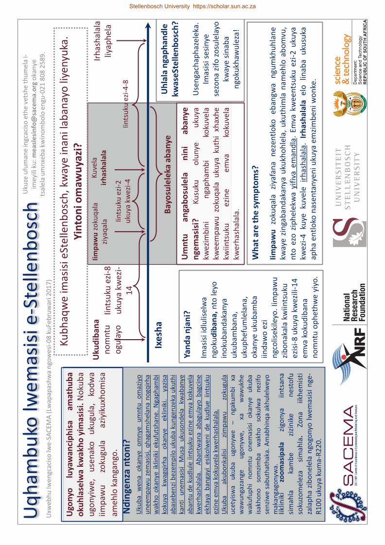
Uku
dib
ana
no
mn
tu
ogu
layo
Iim
paw
u z
oku
qal
a zi
yaq
ala
Kuve
la
irh
ash
alal
a Ir
has
hal
ala
liyap
hel
a
Wh
at a
re t
he
sym
pto
ms?
Ii
mp
awu
zo
kuq
ala
ziya
fan
a n
ezen
tlo
ko
eban
gwa
ngu
mkh
uh
lan
e
kway
e z
inga
ban
dak
anya
uku
kho
hle
la,
uku
thim
la n
ameh
lo a
bo
mvu
, n
to e
zo z
iph
elek
wa
yifi
va e
man
dla
. Em
va k
wee
nts
uku
ezi
-2 u
kuya
kw
ezi-
4
kuye
ku
vele
ir
has
hal
ala.
Ir
has
hal
ala
elo
lin
aba
uku
suka
ap
ha
entl
oko
nas
enta
nye
ni u
kuya
em
zim
ben
i wo
nke
.
Yan
da
nja
ni?
Im
asis
i id
lulis
elw
a n
goku
dib
ana,
nto
leyo
in
oku
ban
dak
anya
u
kub
amb
ana,
u
kup
hef
um
lela
na,
o
kan
ye u
kub
amb
a iin
daw
o e
zi
ngc
olis
ekile
yo. I
imp
awu
zi
bo
nak
ala
kwiin
tsu
ku
ezis
i-8
uku
ya k
wez
ili-1
4
emva
ko
kud
iban
a n
om
ntu
op
het
hw
e y
iyo
.
Iints
uku
ezi
-8
uku
ya k
wez
i-1
4
Iints
uku
ezi
-2
uku
ya k
wez
i-4
Ixe
sha
Um
ntu
an
gab
osu
lela
n
ini
aban
ye
nge
mas
isi?
Ku
suku
o
lun
ye
uku
ya
kwez
imb
ini
nga
ph
amb
i ko
kuve
la
kwee
mp
awu
zo
kuq
ala
uku
ya k
uth
i xh
axh
e
kwiin
tsu
ku
ezin
e
em
va
koku
vela
kw
erh
ash
alal
a.
Bay
osu
lele
ka a
ban
ye
Iints
uku
ezi
-4-8
N
din
gen
za n
ton
i?
Iiklin
iki
zoo
mas
ipal
a zi
gony
a iin
tsan
a si
mah
la
kam
be
zi
zin
ike
n
esto
fu
soku
zom
elez
a si
mah
la.
Zon
a iik
hem
isti
za
lap
ha
zib
on
elel
a n
gogo
nyo
lw
emas
isi
nge
-R
10
0 u
kuya
ku
ma-
R2
20
.
Ugo
nyo
lu
yaw
anci
ph
isa
amat
hu
ba
oku
hla
selw
a kw
akh
o y
imas
isi.
No
kub
a u
gon
yiw
e,
use
nak
o
uku
gula
, ko
dw
a iim
paw
u
zoku
gula
az
iyik
uxh
om
isa
ameh
lo k
anga
ngo
.
Uku
ba
wen
a o
kan
ye
om
nye
u
mn
tu
om
aziy
o
un
eem
paw
u z
emas
isi,
qh
agam
shel
ana
no
gqir
ha
wak
ho
oka
nye
ikl
inik
i ek
ufu
tsh
ane.
Nga
ph
amb
i ko
kuya
kw
agq
irh
a o
kan
ye
eklin
iki.
yazi
sa
abas
eben
zi b
ezem
pilo
uku
ba
kun
gen
zeka
uku
thi
kan
ti
un
emas
isi
Mu
sa
uku
son
del
a kw
aban
ye
aban
tu d
e ku
dlu
le ii
nts
uku
ezi
ne
emva
ko
kuve
la
kwer
has
hal
ala.
A
ban
twan
a ab
agu
layo
bag
cin
e
ekh
aya
ban
gayi
esi
kolw
eni
de
kud
lue
iin
tsu
ku
ezin
e em
va k
oku
vela
kw
erh
ash
alal
a.
Uku
ba
aku
bo
nka
lisi
zim
paw
u
zoku
gula
u
cety
isw
a u
kub
a u
gon
ywe
–
nga
kum
bi
xa
waw
un
gaza
nge
u
gon
ywe,
xa
w
awu
khe
wak
ufu
ph
i n
om
ntu
o
nem
asis
i o
kan
ye
uku
ba
isak
ho
no
so
mzi
mb
a w
akh
o
soku
lwa
nez
ifo
se
nzi
we
sab
uth
ath
aka.
Am
abh
inq
a ak
hu
lelw
eyo
m
akan
gago
nyw
a.
Uxw
ebh
u lw
engc
acis
o lw
e-S
AC
EMA
(Lw
apap
ash
wa
ngo
we
si-0
8 k
uFe
bru
war
i 20
17
)
Uh
lala
nga
ph
and
le
kwas
eSt
elle
nb
osc
h?
U
sen
gach
aph
azel
eka.
Im
asis
i ses
inye
se
zon
a zi
fo z
osu
lela
yo
kway
e si
nab
a n
goku
khaw
ule
za!
Uq
ham
bu
ko lw
emas
isi e
-Ste
llen
bo
sch
Ku
bh
aqw
e im
asis
i eSt
elle
nb
osc
h, k
way
e in
ani l
aban
ayo
liye
nyu
ka.
Yin
ton
i om
awu
yazi
?
Uku
ze u
fum
ane
ingc
acis
o e
the
vet
she
thu
mel
a i-
imey
ili k
u: m
eas
lesi
nfo
@sa
cem
a.o
rg o
kan
ye
tsal
ela
um
nxe
ba
kwin
om
bo
lo e
ngu
-02
1 8
08
25
89
.
Stellenbosch University https://scholar.sun.ac.za

Uq
ham
bu
ko lw
eMas
isi e
-Ste
llen
bo
sch
In
gcac
iso
eth
e v
etsh
e t
hu
mel
a i-
imey
ili k
u:
me
asle
sin
fo@
sace
ma.
org
oka
nye
tsa
lela
ku
: 02
1
80
8 2
58
9.
Iiklin
iki z
oo
mas
ipal
a zi
gon
ya ii
nts
ana
sim
ahla
kam
be
zizi
nik
e n
est
ofu
so
kuzo
mel
eza
sim
ahla
K
han
gela
iklin
iki e
kufu
tsh
ane
ku
we
Clo
ete
svill
e C
om
mu
nit
y H
eal
th C
linic
Te
nn
antv
ille
Stre
et, S
telle
nb
osc
h
02
1 8
83
26
76
Fr
ansc
hh
oe
k Sa
telli
te C
linic
A
kad
emie
Str
eet
Fran
sch
ho
ek
02
1 8
76
21
72
G
roe
nd
al K
linie
k 1
Sti
ebeu
elst
r, F
ran
sch
ho
ek
02
1 8
76
37
14
Id
as V
alle
y C
linic
H
amm
and
shan
d W
ay Id
as V
alle
y, S
telle
nb
osc
h
02
1 8
87
27
21
Jam
est
ow
n C
linic
Pa
jero
Str
eet,
Jam
esto
wn
, Ste
llen
bo
sch
0
21
88
0 0
35
7
K
ayam
and
i Clin
ic
56
Bas
si S
tree
t, K
ayam
and
i, St
elle
nb
osc
h
02
1 8
89
50
61
K
yle
mo
re C
linic
1
9 S
cho
ol S
tree
t, K
ylem
ore
0
21
88
5 2
50
4
R
ho
de
s Fr
uit
Far
m C
linic
G
roo
t D
rake
nst
ein
, 76
80
0
21
87
4 1
11
2
Som
ers
et W
est
Clin
ic
28
Ch
urc
h S
tree
t, S
om
erse
t W
est
02
1 4
44
44
52
V
icto
ria
Stre
et C
linic
5
Vic
tori
a St
reet
, Ste
llen
bo
sch
0
21
88
7 2
65
0
Ab
antu
ab
amiz
imb
a is
akh
on
o
soku
lwa
nez
ifo
si
bu
that
hak
a –
kub
and
akan
ywa
iints
na
nab
antu
ab
aph
ila
ne-
HIV
–
nga
bo
na
bas
emn
gcip
hek
we
ni
wo
kub
a n
een
gxak
i ez
ino
koya
nya
nis
wa
no
kosu
lelw
a yi
mas
isi.
Ab
o
ban
tu
bac
etyi
swa
kakh
ulu
u
kub
a b
ago
nyw
e.
Am
abh
inq
a am
aith
iyo
mak
anga
gon
ywa.
.
Uxw
ebh
u lw
engc
acis
o lw
e-S
AC
EMA
(Lw
apap
ash
wa
ngo
we
si-0
8 k
uFe
bru
war
i 20
17
)
Stellenbosch University https://scholar.sun.ac.za

Appendix A. 92
A.2 Epidemic update sheet in English
Stellenbosch University https://scholar.sun.ac.za
List of references
Aaby, P., Knudsen, K., Jensen, T.G., Thirup, J., Poulsen, A., Sodemann, M., da Silva, M.C.& Whittle, H. 1990. Measles incidence, vaccine efficacy, and mortality in two urbanAfrican areas with high vaccination coverage. Journal of infectious diseases, 162(5):1043–1048.
Anderson, R.M., May, R.M. & Anderson, B. 1992. Infectious diseases of humans: dynamicsand control, volume 28. Wiley Online Library.
Aylward, R.B., Clements, J. & Olive, J.-M. 1997. The impact of immunization controlactivities on measles outbreaks in middle and low income countries. Internationaljournal of epidemiology, 26(3):662–669.
Bailey, N.T. 1975. The mathematical theory of infectious diseases and its applications. CharlesGriffin & Company Ltd, 5a Crendon Street, High Wycombe, Bucks HP13 6LE.
Becker, A.D. & Grenfell, B.T. 2017. tsir: An R package for time-series susceptible-infected-recovered models of epidemics. PloS one, 12(9):e0185528.
Bellan, S.E., Pulliam, J.R., Pearson, C.A., Champredon, D., Fox, S.J., Skrip, L., Galvani,A.P., Gambhir, M., Lopman, B.A., Porco, T.C. et al.. 2015. Statistical power and validityof ebola vaccine trials in Sierra Leone: a simulation study of trial design and analysis.The Lancet Infectious Diseases, 15(6):703–710.
Biellik, R., Madema, S., Taole, A., Kutsulukuta, A., Allies, E., Eggers, R., Ngcobo, N., Nx-umalo, M., Shearley, A., Mabuzane, E. et al.. 2002. First 5 years of measles eliminationin Southern Africa: 1996–2000. The Lancet, 359(9317):1564–1568.
Bjørnstad, O.N., Finkenstädt, B.F. & Grenfell, B.T. 2002. Dynamics of measles epidemics:estimating scaling of transmission rates using a time series sir model. Ecological Mono-graphs, 72(2):169–184.
93
Stellenbosch University https://scholar.sun.ac.za
List of references 94
Black, R.E., Cousens, S., Johnson, H.L., Lawn, J.E., Rudan, I., Bassani, D.G., Jha, P.,Campbell, H., Walker, C.F., Cibulskis, R. et al.. 2010. Global, regional, and nationalcauses of child mortality in 2008: a systematic analysis. The lancet, 375(9730):1969–1987.
Blake, F.G. & Trask Jr, J.D. 1921. Studies on measles: III. acquired immunity followingexperimental measles. The Journal of experimental medicine, 33(5):621.
Bobashev, G.V., Ellner, S.P., Nychka, D.W. & Grenfell, B.T. 2000. Reconstructing suscep-tible and recruitment dynamics from measles epidemic data. Mathematical PopulationStudies, 8(1):1–29.
Bolker, B. & Grenfell, B. 1993. Chaos and biological complexity in measles dynamics.Proceedings of the Royal Society of London B: Biological Sciences, 251(1330):75–81.
Cairns, K.L., Perry, R.T., Ryman, T.K., Nandy, R.K. & Grais, R.F. 2011. Should outbreakresponse immunization be recommended for measles outbreaks in middle-and low-income countries? an update. The Journal of infectious diseases, 204(suppl_1):S35–S46.
Chang, W., Cheng, J., Allaire, J., Xie, Y. & McPherson, J. 2017. Shiny: Web ApplicationFramework for R. R package version 1.0.5.Available at: https://CRAN.R-project.org/package=shiny
Chiew, M., Gidding, H.F., Dey, A., Wood, J., Martin, N., Davis, S. & McIntyre, P. 2014.Estimating the measles effective reproduction number in Australia from routine noti-fication data. Bulletin of the World Health Organization, 92(3):171–177.
Cori, A., Ferguson, N.M., Fraser, C. & Cauchemez, S. 2013. A new framework andsoftware to estimate time-varying reproduction numbers during epidemics. Americanjournal of epidemiology, 178(9):1505–1512.
Dalziel, B.D., Bjørnstad, O.N., van Panhuis, W.G., Burke, D.S., Metcalf, C.J.E. & Gren-fell, B.T. 2016. Persistent chaos of measles epidemics in the prevaccination UnitedStates caused by a small change in seasonal transmission patterns. PLoS computationalbiology, 12(2):e1004655.
De Swart, R. 2009. Measles studies in the macaque model. Curr Top Microbiol Immunol,330:55–72.
Dorélien, A.M., Ballesteros, S. & Grenfell, B.T. 2013. Impact of birth seasonality on dy-namics of acute immunizing infections in sub-Saharan Africa. PLoS One, 8(10):e75806.
Stellenbosch University https://scholar.sun.ac.za
95 List of references
Earn, D.J., Rohani, P., Bolker, B.M. & Grenfell, B.T. 2000. A simple model for complexdynamical transitions in epidemics. Science, 287(5453):667–670.
Enders, J.F., Katz, S.L. & Holloway, A. 1962. Development of attenuated measles virusvaccines: A summary of recent investigation. American Journal of Diseases of Children,103(3):335–340.
Ferrari, M.J., Bjørnstad, O.N. & Dobson, A.P. 2005. Estimation and inference of R0 of aninfectious pathogen by a removal method. Mathematical biosciences, 198(1):14–26.
Ferrari, M.J., Fermon, F., Nackers, F., Llosa, A., Magone, C. & Grais, R.F. 2014. Timeis (still) of the essence: quantifying the impact of emergency meningitis vaccinationresponse in Katsina State, Nigeria. International health, 6(4):282–290.
Ferrari, M.J., Grais, R.F., Bharti, N., Conlan, A.J., Bjørnstad, O.N., Wolfson, L.J., Guerin,P.J., Djibo, A. & Grenfell, B.T. 2008. The dynamics of measles in sub-Saharan Africa.Nature, 451(7179):679–684.
Fine, P.E. 2003. The interval between successive cases of an infectious disease. Americanjournal of epidemiology, 158(11):1039–1047.
Fine, P.E. & Clarkson, J.A. 1982. Measles in England and Wales–I: an analysis of factorsunderlying seasonal patterns. International journal of Epidemiology, 11(1):5–14.
Finkenstädt, B.F. & Grenfell, B.T. 2000. Time series modelling of childhood diseases: adynamical systems approach. Journal of the Royal Statistical Society: Series C (AppliedStatistics), 49(2):187–205.
Fulginiti, V. 1965. Simultaneous measles exposure and immunization. Archives of Virol-ogy, 16(1):300–304.
Glass, K. & Grenfell, B. 2003. Antibody dynamics in childhood diseases: waning andboosting of immunity and the impact of vaccination. Journal of theoretical biology,221(1):121–131.
Grais, R., De Radiguès, X., Dubray, C., Fermon, F. & Guerin, P. 2006a. Exploring thetime to intervene with a reactive mass vaccination campaign in measles epidemics.Epidemiology & Infection, 134(4):845–849.
Stellenbosch University https://scholar.sun.ac.za
List of references 96
Grais, R.F., Conlan, J.K., Ferrari, M.J., Djibo, A., Le Menach, A., Bjørnstad, O.N. & Gren-fell, B.T. 2007. Time is of the essence: exploring a measles outbreak response vaccina-tion in Niamey, Niger. Journal of the Royal Society, Interface / the Royal Society, 5(18):67–74. ISSN 1742-5689.
Grais, R.F., Ferrari, M., Dubray, C., Bjørnstad, O., Grenfell, B., Djibo, A., Fermon, F.& Guerin, P.J. 2006b. Estimating transmission intensity for a measles epidemic inNiamey, Niger: lessons for intervention. Transactions of the Royal Society of TropicalMedicine and Hygiene, 100(9):867–873.
Grenfell, B.T., Bjørnstad, O.N. & Finkenstädt, B.F. 2002. Dynamics of measles epidemics:scaling noise, determinism, and predictability with the tsir model. Ecological Mono-graphs, 72(2):185–202.
Griffin, D. & Pan, C.-H. 2009. Measles: old vaccines, new vaccines. In Measles, pages191–212. Springer.
Griffin, D.E. & Oldstone, M.B. 2008. Measles: Pathogenesis and control, volume 330.Springer Science & Business Media.
Guerra, F.M., Bolotin, S., Lim, G., Heffernan, J., Deeks, S.L., Li, Y. & Crowcroft, N.S.2017. The basic reproduction number (R0) of measles: a systematic review. The LancetInfectious Diseases. ISSN 1473-3099.Available at: http://dx.doi.org/10.1016/S1473-3099(17)30307-9
Halloran, M.E., Auranen, K., Baird, S., Basta, N.E., Bellan, S., Brookmeyer, R., Cooper,B., DeGruttola, V., Hughes, J., Lessler, J. et al.. 2017. Simulations for designing andinterpreting intervention trials in infectious diseases. bioRxiv, page 198051.
Heffernan, J. & Keeling, M.J. 2008. An in-host model of acute infection: Measles as acase study. Theoretical population biology, 73(1):134–147.
Heymann, D.L. 2004. Control of communicable diseases manual 18th Edition. AmericanPublic Health Association.
Hobson, F. 1934. The use of convaslescent measles serum in school epidemics. TheLancet, 224(5808):1408–1411.
Hobson, F. 1938. Measles: The conduct of a school epidemic. The British Medical Journal,pages 171–175.
Stellenbosch University https://scholar.sun.ac.za
97 List of references
Keeling, M.J. & Grenfell, B. 1997. Disease extinction and community size: modeling thepersistence of measles. Science, 275(5296):65–67.
Keeling, M.J. & Rohani, P. 2008. Modeling infectious diseases in humans and animals. Prince-ton University Press.
Klepac, P., Bjørnstad, O.N., Metcalf, C.J.E. & Grenfell, B.T. 2012. Optimizing reactiveresponses to outbreaks of immunizing infections: balancing case management andvaccination. PloS one, 7(8):e41428.
Krugman, S., Giles, J.P., Friedman, H. & Stone, S. 1965. Studies on immunity to measles.The Journal of pediatrics, 66(3):471–488.
Lessler, J., Metcalf, C.J.E., Cutts, F.T. & Grenfell, B.T. 2016. Impact on epidemic measlesof vaccination campaigns triggered by disease outbreaks or serosurveys: a modelingstudy. PLoS medicine, 13(10):e1002144.
Markowitz, L.E., Preblud, S.R., Fine, P.E. & Orenstein, W.A. 1990. Duration of livemeasles vaccine-induced immunity. The Pediatric infectious disease journal, 9(2):101–110.
Metcalf, C., Lessler, J., Klepac, P., Cutts, F. & Grenfell, B. 2012. Impact of birth rate,seasonality and transmission rate on minimum levels of coverage needed for rubellavaccination. Epidemiology & Infection, 140(12):2290–2301.
Metcalf, C.J.E., Bjørnstad, O.N., Grenfell, B.T. & Andreasen, V. 2009. Seasonality andcomparative dynamics of six childhood infections in pre-vaccination Copenhagen.Proceedings of the Royal Society of London B: Biological Sciences, 276(1676):4111–4118.
Minetti, A., Hurtado, N., Grais, R.F. & Ferrari, M. 2013. Reaching hard-to-reach in-dividuals: nonselective versus targeted outbreak response vaccination for measles.American journal of epidemiology, 179(2):245–251.
Moss, W.J. & Griffin, D.E. 2012. Measles review article, Moss & Griffin. The Lancet,379:153–164.
Mossong, J. & Muller, C.P. 2003. Modelling measles re-emergence as a result of waningof immunity in vaccinated populations. Vaccine, 21(31):4597–4603.
Mossong, J., Nokes, D.J., Edmunds, W.J., Cox, M.J., Ratnam, S. & Muller, C.P. 1999.Modeling the impact of subclinical measles transmission in vaccinated populationswith waning immunity. American Journal of Epidemiology, 150(11):1238–1249.
Stellenbosch University https://scholar.sun.ac.za
List of references 98
Orenstein, W.A. & Gay, N.J. 2004. The theory of measles elimination: implica-tions for the design of elimination strategies. The Journal of infectious diseases,189(Supplement_1):S27–S35.
Orenstein, W.A., Perry, R.T. & Halsey, N.A. 2004. The clinical significance of measles: areview. The Journal of infectious diseases, 189(Supplement_1):S4–S16.
Perry, R.T., Gacic-Dobo, M., Dabbagh, A., Mulders, M.N., Strebel, P.M., Okwo-Bele, J.-M., Rota, P.A., Goodson, J.L. et al.. 2014. Progress toward regional measles eliminationworldwide, 2000–2013. MMWR Morb Mortal Wkly Rep, 63(45):1034–8.
Pinner, R.W., Onyango, F., Perkins, B.A., Mirza, N.B., Ngacha, D.M., Reeves, M., DeWitt,W., Njeru, E., Agata, N.N., Broome, C.V. et al.. 1992. Epidemic meningococcal diseasein Nairobi, Kenya, 1989. Journal of infectious diseases, 166(2):359–364.
R Core Team. 2017. R: A Language and Environment for Statistical Computing. Vienna,Austria.Available at: https://www.R-project.org/
Shibeshi, M.E., Masresha, B.G., Smit, S.B., Biellik, R.J., Nicholson, J.L., Muitherero, C.,Shivute, N., Walker, O., Reggis, K. & Goodson, J.L. 2014. Measles resurgence in South-ern Africa: challenges to measles elimination. Vaccine, 32(16):1798–1807.
Uzicanin, A. & Zimmerman, L. 2011. Field effectiveness of live attenuated measles-containing vaccines: a review of published literature. The Journal of infectious diseases,204(suppl_1):S133–S149.
Wallinga, J., Levy-Bruhl, D., Gay, N. & Wachmann, C. 2001. Estimation of measles re-production ratios and prospects for elimination of measles by vaccination in someWestern European countries. Epidemiology & Infection, 127(2):281–295.
WHO. 1999. WHO guidelines for epidemic preparedness and response to measles out-breaks.
WHO. 2005. Givs: global immunization vision and strategy: 2006-2015.
WHO. 2009. Response to measles outbreaks in measles mortality reduction settings.
WHO. 2017. Measles vaccines: WHO position paper (april 2017). Weekly EpidemiologicalRecord, 92(17):205–227.Available at: http://apps.who.int/iris/bitstream/10665/255377/1/
WER9217-205-227.pdf
Stellenbosch University https://scholar.sun.ac.za

99 List of references
Yeung, L.F., Lurie, P., Dayan, G., Eduardo, E., Britz, P.H., Redd, S.B., Papania, M.J. &Seward, J.F. 2005. A limited measles outbreak in a highly vaccinated US boardingschool. Pediatrics, 116(6):1287–1291.
Stellenbosch University https://scholar.sun.ac.za