Assessment of a Hybrid Retrofit Gas Water Heater · Assessment of a Hybrid Retrofit Gas Water...
77
Assessment of a Hybrid Retrofit Gas Water Heater Marc Hoeschele, Elizabeth Weitzel, and Christine Backman Alliance for Residential Building Innovation February 2017
Transcript of Assessment of a Hybrid Retrofit Gas Water Heater · Assessment of a Hybrid Retrofit Gas Water...

Assessment of a Hybrid Retrofit Gas Water Heater Marc Hoeschele, Elizabeth Weitzel, and Christine Backman Alliance for Residential Building Innovation
February 2017

iii
NOTICE
This report was prepared as an account of work sponsored by an agency of the United States government. Neither the United States government nor any agency thereof, nor any of their employees, subcontractors, or affiliated partners makes any warranty, express or implied, or assumes any legal liability or responsibility for the accuracy, completeness, or usefulness of any information, apparatus, product, or process disclosed, or represents that its use would not infringe privately owned rights. Reference herein to any specific commercial product, process, or service by trade name, trademark, manufacturer, or otherwise does not necessarily constitute or imply its endorsement, recommendation, or favoring by the United States government or any agency thereof. The views and opinions of authors expressed herein do not necessarily state or reflect those of the United States government or any agency thereof.
This report is available at no cost from the National Renewable Energy Laboratory (NREL) at www.nrel.gov/publications.
Available electronically at SciTech Connect http:/www.osti.gov/scitech
Available for a processing fee to U.S. Department of Energy and its contractors, in paper, from:
U.S. Department of Energy Office of Scientific and Technical Information P.O. Box 62 Oak Ridge, TN 37831-0062 OSTI http://www.osti.gov Phone: 865.576.8401 Fax: 865.576.5728 Email: [email protected]
Available for sale to the public, in paper, from: U.S. Department of Commerce National Technical Information Service 5301 Shawnee Road Alexandria, VA 22312 NTIS http://www.ntis.gov Phone: 800.553.6847 or 703.605.6000 Fax: 703.605.6900 Email: [email protected]

iii
Assessment of a Hybrid Retrofit Gas Water Heater
Prepared for:
The National Renewable Energy Laboratory
On behalf of the U.S. Department of Energy’s Building America Program
Office of Energy Efficiency and Renewable Energy
15013 Denver West Parkway
Golden, CO 80401
NREL Contract No. DE-AC36-08GO28308
Prepared by:
Marc Hoeschele, Elizabeth Weitzel, and Christine Backman
Alliance for Residential Building Innovation
Davis Energy Group, Team Lead
123 C Street
Davis, CA 95616
NREL Technical Monitor: Stacey Rothgeb
Prepared under Subcontract No. KNDJ-0-40340-04
February 2017

iv
The work presented in this report does not represent performance of any product relative to regulated minimum efficiency requirements.
The laboratory and/or field sites used for this work are not certified rating test facilities. The conditions and methods under which products were characterized for this work differ from standard rating conditions, as described.
Because the methods and conditions differ, the reported results are not comparable to rated product performance and should only be used to estimate performance under the measured conditions.

v
Contents List of Figures ............................................................................................................................................ vi List of Tables .............................................................................................................................................. vi Definitions .................................................................................................................................................. vii Executive Summary ................................................................................................................................. viii 1 Introduction ........................................................................................................................................... 1
1.1 Background and Motivation ............................................................................................................ 1 1.2 Research Questions .......................................................................................................................... 5
2 Methodology ......................................................................................................................................... 6 2.1 Storage Water Heater Model ........................................................................................................... 6 2.2 Basic Tankless Water Heater Model ................................................................................................ 8 2.3 Original Equipment Manufacturer Hybrid Water Heater Model ..................................................... 9 2.4 Alternative Hybrid Water Heater Model ....................................................................................... 11 2.5 Other Model Assumptions ............................................................................................................. 12
3 Results ................................................................................................................................................. 15 3.1 Calibration of Base Water Heater Models ..................................................................................... 15 3.2 Peak Day Performance Simulations To Determine Hybrid Tank Sizing ....................................... 15 3.3 Evaluating Peak Day Performance for Alternative Water Heater Designs .................................... 16 3.4 Annual Performance Simulations .................................................................................................. 17 3.5 Preliminary Economic Assessment ................................................................................................ 22
4 Conclusions ........................................................................................................................................ 24 References ................................................................................................................................................. 26 Appendix A: Storage Type 534 and Tankless Type 940 Water Heater Model Descriptions .............. 27 Appendix B: Alternative Peak Day Hot Water Draw Profiles ................................................................ 51 Appendix C: TRNSYS Single Day (183GPD) Hybrid Optimization Run Result Summary ................. 62 Appendix D: TRNSYS Annual Run Result Summary ............................................................................ 63

vi
List of Figures Figure 1. Distribution of gas water heaters by EF rating ........................................................................ 2 Figure 2. Summary of hot water draw characteristics from the 159-home data set ............................ 5 Figure 3. Schematic representation of storage water heater ................................................................. 7 Figure 4. Tankless model (TRNSYS Type 940) control diagram ............................................................ 8 Figure 5. Hybrid water heater storage tank schematic ......................................................................... 10 Figure 6. Basic hybrid system schematic .............................................................................................. 11 Figure 7. Design day hot water draw profile (183 gpd) ......................................................................... 13 Figure 8. Hybrid tank size influence on site efficiency and thermal loss ........................................... 16 Figure 9. Annual system site efficiency as a function of hot water draw volume and climate ......... 19 Figure 10. Range in average annual system site efficiencies across all scenarios .......................... 20 Figure 11. Comparison of Minneapolis annual site energy use to wasted water (gallons) .............. 21 Figure 12. Comparison of Sacramento annual site energy use to wasted water (gallons) ............... 21 Figure 13. Comparison of Phoenix annual site energy use to wasted water (gallons) ..................... 22 Unless otherwise indicated, all figures were created by the Alliance for Residential Building Innovation team.
List of Tables Table 1. Projected Alternative Hybrid Energy and Cost Impacts by Climate ...................................... ix Table 2. Minimum EF Requirements under Previous and Current Standards ...................................... 1 Table 3. Atmospheric Gas Storage Water Heater Model Input Assumptions ....................................... 7 Table 4. Tankless Water Heater Model Inputs .......................................................................................... 9 Table 5. OEM Hybrid Water Heater Model Inputs................................................................................... 10 Table 6. Alternative Hybrid Water Heater Model Assumed Inputs ....................................................... 12 Table 7. Pre-2015 DOE EF Water Heater Test Standard Conditions .................................................... 15 Table 8. TRNSYS Projected Simulated Energy Factor .......................................................................... 15 Table 9. Minneapolis Results for a High Consumption Day in February (183 gpd) ........................... 17 Table 10. Annual Projected System Efficiencies for Minneapolis ....................................................... 18 Table 11. Annual Simulated Results for Minnesota One-Bedroom Case ............................................ 18 Table 12. Annual Simulated Results for Minnesota Five-Bedroom Case ........................................... 22 Table 13. Performance and Operating Cost Comparison as a Function of Load and Climate ......... 23 Table 14. TRNSYS Summary for One-Bedroom (36 gpd) Minneapolis ................................................ 63 Table 15. TRNSYS Summary for Two-Bedroom (57 gpd) Minneapolis ............................................... 63 Table 16. TRNSYS Summary for Five-Bedroom (92 gpd) Minneapolis ............................................... 64 Table 17. TRNSYS Summary for One-Bedroom (36 gpd) Sacramento ................................................ 64 Table 18. TRNSYS Summary for Two-Bedroom (57 gpd) Sacramento ................................................ 65 Table 19. TRNSYS Summary for Five-Bedroom (92 gpd) Sacramento ................................................ 65 Table 20. TRNSYS Summary for One-Bedroom (36 gpd) Phoenix ...................................................... 66 Table 21. TRNSYS Summary for Two-Bedroom (57 gpd) Phoenix ...................................................... 66 Table 22. TRNSYS Summary for Five-Bedroom (92 gpd) Phoenix ...................................................... 67 Unless otherwise indicated, all tables were created by the Alliance for Residential Building Innovation team.

vii
Definitions
DHWESG Domestic Hot Water Event Schedule Generator
DOE U.S. Department of Energy
EIA Energy Information Administration
EF Energy Factor
gpd Gallons per Day
gpm Gallons per Minute
GTI Gas Technology Institute
HOT Hybrid Optimized Tankless
kBtu Thousand British Thermal Units
kW Kilowatt, Electricity Demand
kWh Kilowatt-Hour
OEM Original Equipment Manufacturer
TESS Thermal Energy Simulation Specialists
TRNSYS TRaNsient System Simulation program

viii
Executive Summary
According to the most recent 2009 data from the U.S. Department of Energy’s (DOE’s) Energy Information Administration (EIA), residential water heating energy consumption equaled 1.8 quadrillion Btu annually. The 1.8 quads of energy represent slightly less than 18% of the energy consumed in residential buildings, which is virtually identical to the 1993 level. According to DOE’s Building Technologies Office, the April 2015 adoption of higher minimum residential water heater efficiencies will save approximately 3.3 quads of energy from 2015–2044.1 To put the 30-year 3.3-quad savings into perspective, the annualized 0.11-quad savings represent a 6% reduction from 2009 water heating consumption.
Commonly available efficient gas water heating options include condensing gas storage units and condensing and noncondensing tankless units. Tankless market share is rising rapidly; much of the impact is realized in new construction. Tankless retrofits are not uncommon, but they are often hindered by significant costs associated with upsizing gas lines (from the typical ½-in. line that commonly serves gas storage water heaters), changing from the standard Category I/Type B vent to polyvinyl chloride or stainless vent pipe, and adding electrical service to power the unit. These costs can easily add $1,000 or more depending upon site conditions. DOE’s 2014 Water Heating Roadmap identifies the challenge of retrofitting affordable and efficient water heaters as a key barrier, because many water heaters are replaced in emergency situations during which delays in replacement represent significant inconveniences.
DOE’s Building America research team Alliance for Residential Building Innovation completed a modeling evaluation of a hybrid gas water heater that combines a reduced capacity tankless unit with a smaller storage tank to assess performance impacts.2 This product would meet a significant market need by providing a higher-efficiency gas water heater for retrofit applications that is compatible with the typical ½-in. gas lines and standard B vents that are found in most homes.
The TRaNsient System Simulation model was used to project performance of a base-case 0.60 energy factor (EF) atmospheric gas storage water heater, a 0.82 EF gas tankless water heater, a high-capacity hybrid unit on the market, and an alternative hybrid unit with lower storage volume and reduced gas input requirements. Simulations were completed under a “peak-day” sizing scenario with 183-gpd hot water loads in a Minnesota winter climate case. A 20-gallon storage tank with 75-kBtu/h input capacity and an 83% assumed combustion efficiency (the upper limit on efficiency to avoid condensing of flue gases) provided adequate hot water delivery under these extreme load conditions.
Annual simulations were then completed in three climates (Phoenix, Sacramento, and Minneapolis) for three representative load scenarios (36, 57, and 96 gpd). Model projections indicate that the alternative hybrid offers an average 4.5% efficiency improvement relative to the 0.60 EF gas storage unit across all scenarios modeled. The greatest projected efficiency benefit (9% improvement) was achieved for the low-load Phoenix scenario. Any projected hot water
1 http://www1.eere.energy.gov/buildings/appliance_standards/product.aspx/productid/27 2 Not to be confused with a hybrid electric (or heat pump water heater), the gas hybrid evaluated here combines downsized storage volume with a lower Btu input tankless unit.

ix
delivery shortcomings of the alternative hybrid that were observed in the cold Minneapolis climate were eliminated under this scenario. Table 1 shows projected gas savings, site energy savings, and operating cost savings for the alternative hybrid unit assuming national average electricity and gas rates. The climate variability shown is due to the impact of the hot water load assumptions. The highest savings are projected for the lowest hot water loads. Site energy savings are diminished relative to the gas savings because electricity consumption was added for the hybrid unit. Cost savings are further negatively impacted by the relative pricing of electricity and natural gas.
Table 1. Projected Alternative Hybrid Energy and Cost Impacts by Climate
* At national average rates of $0.1212/kWh and $1.003/therm The alternative hybrid water heater that was evaluated shows promise. However, the cost of natural gas is generally low and the incremental efficiency improvement is relatively slight; thus, marketing this product in a competitive gas water heater marketplace may be challenging. Additional laboratory testing and optimization would be valuable to further document performance and to determine if savings can be improved with lower parasitic energy use and improved control strategies that optimize the impact of the downsized storage in handling peak hot water load events. The alternative hybrid unit evaluated in this study is likely best suited for warmer climates and smaller homes in which peak hot water loads would be lower and the impact of reduced standby losses is more significant.
Climate Natural Gas
Savings (therm/yr)
Natural Gas Savings
(%)
Site Energy Savings
(%)
Annual Cost Savings
($)* Cold—Minneapolis 17–21 5–12 4–10 0–9
Moderate—Sacramento 14–20 5–15 4–13 0–11 Hot—Phoenix 14–20 7–18 5–17 1–12

1
1 Introduction
1.1 Background and Motivation According to the U.S Department of Energy’s (DOE’s) Energy Information Administration (EIA)3 residential water heating energy consumption equaled 1.8 quadrillion Btu annually based on the most recent 2009 data. The 1.8 quads of energy represent slightly less than 18% of the energy consumed in residential buildings and are virtually identical to the estimated consumption level for water heating in 1993. Over the same 1993–2009 time period, EIA-projected heating and cooling energy use for all residential buildings declined by 16%.
The recent adoption of higher minimum residential water heater efficiencies (effective April 1, 2015)4 results in increased energy factors (EFs) as summarized in Table 2. (Pre-April 1, 2015, and current minimum EFs are shown for an example storage volume to provide a sense of the efficiency level changes for typical water heater sizes.) The new standards will certainly impact future water heating energy savings, especially for gas and electric storage water heaters with volumes larger than 55 gallons. Under the new standards, gas-fired water heaters larger than 55 gallons are required to be condensing water heaters, and electric water heaters larger than 55 gallons will need to implement heat pump technology.5 According to DOE’s Building Technologies Office,6 the April 2015 standards will “save approximately 3.3 quads of energy and result in approximately $63 billion in energy bill savings for products shipped from 2015-2044. The standard will avoid about 172.5 million metric tons of carbon dioxide emissions, equivalent to the annual greenhouse gas emissions of about 33.8 million automobiles.” Averaged over the 30-year time horizon, the 3.3 quads of savings result in annualized savings of 0.11 quads, or 6% of 2009 national water heating consumption.
Table 2. Minimum EF7 Requirements under Previous and Current Standards
Nationwide, 51% of water heaters use natural gas and 41% use electricity; propane and fuel oil make up the bulk of the remaining stock (Goetzler et al. 2014). Even though heat pump water 3 http://www.eia.gov/consumption/residential/ (accessed March 3, 2015) 4 As documented in the Code of Federal Regulations, 10 CFR 430.32(d) 5 Instantaneous, or tankless gas fired water heaters show an apparent significant efficiency increase with the new standards as well; however, virtually all existing gas instantaneous water heaters already meet the new standard. 6 http://www1.eere.energy.gov/buildings/appliance_standards/product.aspx/productid/27 7 Complicating matters further, in July 2014 DOE published a change in the water heater test procedure that separates residential and small commercial water heaters into four usage categories. Testing will involve more realistic draw patterns and determination of a uniform energy factor. Voluntary use of the uniform energy factor begins in July 2015; mandatory use of the uniform energy factor metric begins approximately 1 year later.
Water Heater Type Volume
Threshold (gal)
Example Volume
(gal)
Pre-April 2015
Minimum EF
Current Minimum EF
Gas-Fired Storage 40 0.59 0.62 Gas-Fired Storage >55 65 0.55 0.75 Electric Storage 50 0.90 0.95 Electric Storage >55 80 0.86 1.97
Instantaneous Gas-Fired Water Heater <2 0 0.62 0.82

2
heaters constitute a significant efficiency boost over current electric storage water heaters, the gas water heater savings opportunities are more limited as demonstrated by the range of product offerings identified in the California Energy Commission listing of certified appliances.8 The vast majority of products can be found with efficiencies up to 0.62 EF; another smaller grouping of ENERGY STAR®-certified storage water heaters are in the 0.67–0.70 EF range. No certified products have 0.70 or greater EF. Gas tankless water heaters, both noncondensing and condensing, represent the vast majority of the products at the high end of the performance range.9
Figure 1. Distribution of gas water heaters by EF rating
Tankless water heaters represent a technology that offers energy savings potential for the gas water heater market; expected savings are 30%–38% (Schoenbauer et al. 2011; Hoeschele and Weitzel 2013). According to a presentation at the 2011 American Council for Energy Efficiency Hot Water Forum (Parker 2011), gas tankless water heater sales at that time were approximately 400,000 units per year, or roughly 10% of annual natural gas water heater sales. Parker indicated that tankless sales were increasing at a faster rate than gas storage water heater sales, especially in the condensing tankless area. Some regions of the country are showing this trend to an even greater extent. According to KEMA et al. (2010), the percentage of gas tankless water heaters installed in new California homes increased from 0% in homes built under the 1995 Title 24 standards to 24% in homes built under the 2005 standards. This trend has most likely continued because the combination of an aggressive California Title 24 energy code and statewide utility 8 This listing includes products that would no longer meet the April 2015 efficiency minimums. 9 Some condensing storage products are starting to appear, such as http://www.rheem.com/product/residential-gas-water-heaters-professional-prestige-series-high-efficiency-condensing-power-direct-vent.
0
200
400
600
800
1000
1200
1400
1600
0.58
0.60
0.62
0.64
0.66
0.68
0.70
0.72
0.74
0.76
0.78
0.80
0.82
0.84
0.86
0.88
0.90
0.92
0.94
0.96
Num
ber o
f List
ed P
rodu
cts
with
in E
F Bi
n
Energy Factor (EF)

3
incentive programs (for construction levels that exceed the code minimum) makes tankless water heaters attractive for many builders.
Despite the increasing impact of tankless in the U.S. market, much of the benefit is realized in new construction. Tankless retrofits are not uncommon, but they are often hindered by significant costs associated with upsizing gas lines from the typical ½-in. line common to storage water heaters, changing from the standard B vent to polyvinyl chloride or stainless vent pipe, adding electrical service, and potentially dealing with condensate disposal. These costs can easily add $1,000 or more depending upon the site issues that are specific to the installation, such as the ease of installing the venting and the length of gas pipe that needs to be replaced with ¾-in. or larger gas lines. The DOE 2014 water heating roadmap identifies the inability to retrofit affordable and efficient water heaters as a key barrier; many water heaters are replaced in emergency situations in which delays represent significant inconveniences (Goetzler et al. 2014).
An easily retrofitable, low-cost, and efficient gas water heater is clearly important to achieve widespread water heating gas energy savings. The Gas Technology Institute (GTI) identified this need about 7 years ago and developed the Hybrid Optimized Tankless (HOT) concept to try to fill the void between the ENERGY STAR water heater entry efficiency level (0.67 EF) and the 0.80+ EF level for noncondensing tankless water heaters (Glanville et al. 2009). The goal in the HOT project was to further tune these two interrelated parameters (storage and input capacity) to optimize both, increase efficiency, and maintain adequate first-hour rating characteristics. Key identified parameters that affected efficiency included managing stratification, optimizing thermostat location, and control.
Specific design criteria identified in the HOT project included:
Ensuring compatibility with a ½-in. gas line and the ability to use Category I/Type B vents, which were critical to minimizing installation costs
Achieving an annual operating efficiency no more than 5% lower than typical noncondensing tankless water heaters on the market
Attaining target operating efficiencies of 62%–70% for hot water loads larger than 10 gallons/day
Meeting California’s South Coast Air Quality Management District nitrogen oxide emission regulations: 10 ng/Joule nitrogen oxide (or 14 ng/Joule if higher than 75,000 Btu/h firing rate)
Encouraging water conservation and improving user satisfaction by supporting low-flow draws (at a flow rate of 0.3 gpm).
Minimizing the “cold water sandwich” effect (minimum of 100°F exit temperature).
Supporting simultaneous hot water draws for normal residential uses (a 70°F rise at 5 gpm for 3 minutes).
GTI completed laboratory prototype evaluations of varying tankless burner firing rates (50, 75, and 100 kBtu/h) and buffer storage tank volumes (10, 15, 20, or 30 gallons). Project findings suggested that an optimum single firing rate of 75,000 Btu/h coupled with 20 gallons of buffer storage could result in projected efficiency levels of 71-73% after accounting for potential

4
performance improvements including minimizing parasitic electricity loads and slight improvements in combustion efficiency10. GTI concluded that “coupled with its use of existing conventional water heater ½-in. gas lines and Category I/Type B venting in place in most homes, this hybrid water heater potentially provides a more economically viable efficiency upgrade than tankless water heaters in retrofit applications.” The challenge is the standard chicken-and-egg problem of developing a cost-efficient product that can be built in sufficient volume to achieve the retail pricing at which the market will accept the incremental cost premium.
A key aspect of optimizing a hybrid system is balancing the storage sizing and input rating in a manner that would likely satisfy virtually all hot water loads. To quantify this aspect, the HOT project proposed a performance criterion of maintaining a 70°F temperature rise at a flow rate of 5 gpm over a 3-minute period. To drill a little deeper into this specification, the authors reviewed detailed hot water flow data that Lutz et al. (2012) presented. These authors compiled high-resolution hot water field data from 12 studies that represented 159 homes in roughly a dozen states and Canada. These compiled data with more than 1.6 million hot water draw events represent probably the most robust data set of individual hot water draws. The data set includes primarily existing homes; very few were built in the last 10 years, so water-efficient appliances and fixtures presumably had a lower saturation relative to new homes. With this in mind, future new use data from homes with efficient showerheads, fixtures, and appliances would likely demonstrate lower daily average hot water use and flow rates.
The evaluation of the data from the 159 homes involved a statistical method to group households into hot water use “clusters” based on median daily hot water use. Three clusters were defined to group households into small (fewer than 44 gpd), medium (44–80 gpd), and high (more than 80 gpd) hot water groupings. Average hot water use among all sites was 54.5 gpd; the standard deviation was 36.1 gpd. Figure 2 plots average draw volume and average flow rate for each cluster. The individual bars reflect the resulting distribution breakdown of draw volume (or flow rate) data. For example, in the low-use cluster flow rate case, the 50% (median rate) was 1.2 gpm; the 98th percentile case shows that only 2% of draws exceeded a flow rate of 3.3 gpm. Interestingly in terms of the flow rate data, the distribution is fairly consistent among the three clusters. In terms of hot water draw volume distribution, higher-use households tend to have larger average draw volumes. Two key insights emerged from these results:
For typical households a very small percentage of hot water draws dictates design condition performance.
Intelligent water heating controls (such as anticipatory tank overheating) could help to provide adequate performance without oversizing storage and input capacity.
Commercially available hybrid products include the Grand Hall Eternal Hybrid water heater (developed in 2006), the AO Smith NEXT (introduced in 2010), and the recently introduced Rinnai RH-180. The RH-180 is of particular interest, because it was designed to be compatible with most ½-in. gas lines and can use a 4-in. Category I/Type B vent. The RH-180 unit features a two-stage burner (59 and 91 kBtu/h) and 40 gallons of storage, which suggest that the product
10 The HOT report refers to expected EF values. Since performance of the unit with all the suggested improvement options was not evaluated in accordance with DOE test requirements, the authors have reported expected annual in situ efficiency and these values are not directly comparable to rated EF values.

5
niche is higher-capacity applications. Internet blog postings suggest this unit’s wholesale price is about $1,800.
Figure 2. Summary of hot water draw characteristics from the 159-home data set
1.2 Research Questions The primary objective of this project was to evaluate design options and assess performance of a hybrid water heater that is configured to be easily retrofitted in most homes with gas service.
Research questions include the following:
1. What storage volume sizing is needed to provide adequate performance with a 75-kBtu/h input limitation given realistic design-day hot water loads in mild and cold climates?
2. How significant are performance variations with climate and hot water load?
3. How does a hybrid gas water heater compare to a conventional gas storage water heater in providing adequate-quality hot water delivered under varying load conditions?
4. What is the impact of control strategies, such as strategically overheating storage, on efficiency and hot water delivery?
0.0
2.0
4.0
6.0
8.0
10.0
12.0
14.0
16.0
Low Med High Low Med High
Hot W
ater
Dra
w S
ize (g
allo
ns) o
rHo
t Wat
er F
low
Rat
e (g
pm) 2%
10%
25%
50%
75%
90%
98%
Average Draw Volume (gallons) Average Flow Rate (gpm)
6
2 Methodology
The modeling study evaluated hybrid water heating configurations and control options that could lead to annual energy performance that is close to that of a tankless water heater and has the hot water delivery advantages of a storage water heater (immediate hot water delivery and less wasted water at the end-use points). A hybrid system would also mitigate the cold water sandwich effect that can occur with tankless water heaters, in which close-coupled draws and the start-up response to flow result in periods of cold water delivered while the tankless unit completes its firing sequence. The team worked closely with Thermal Energy Simulation Specialists (TESS) to develop a TRaNsient System Simulation (TRNSYS) model that provided flexibility for modeling hybrid systems of different configurations and conventional baseline storage and tankless systems that served as reference performance cases.
To provide high-resolution output data from TRNSYS, all simulations were completed using 6-second simulation time steps to better tabulate “useful” energy as it left the water heater. To compare storage, tankless, and hybrid water heaters, this study defined useful energy delivered as a key performance metric. The presumption is that hot water leaving the water heater that is below some minimum temperature would not be used at the end-use location (unless it was an appliance). In the modeling, an assumption a 105°F11 minimum “useful” temperature leaving the water heater was defined. If the delivery temperature during any 6-second flow interval did not reach 105°F, the water and associated energy were considered to be wasted. This is a conservative assumption in that appliances will not waste water that does not reach some minimum temperature condition.
A first series of TRNSYS runs was completed to evaluate performance under peak day design conditions for a range of storage sizings for a fixed input capacity level. This was done for three climates: Sacramento, California (moderate climate), Minneapolis, Minnesota (cold climate), and Phoenix, Arizona (hot climate).
Once the peak day TRNSYS runs were completed, full-year simulations were performed in the same climates under three hot water load level assumptions. The chosen climates made it necessary to vary some assumptions including water heater location based on typical practices, water heater set points, and incoming mains water temperature.12 One area where the impact of climate severity was accounted for was in the water heater set point selection. In Minneapolis it was assumed to be 130°F; for Phoenix and Sacramento it was assumed to be 125°F.
The water heater configurations developed in this study are reviewed in Section 2.1 through Section 2.4.
2.1 Storage Water Heater Model The standard atmospheric storage water heater was modeled with the Type 534 model (TESS 2010). The Type 534 model allows for either indirect heating of the storage tank or for direct energy input at one of the nodes defined in the tank. In this modeling effort, five equally sized 11 This assumption is subjective and depends highly on human behaviors in how hot water is used or wasted. 12 The study did not look at varying water heating demands as a function of climate. This effect would further diminish hot climate water heating recovery load as some sink end uses that may require hot water in a cold climate, do not require hot water in a hot climate.

7
isothermal nodes were modeled with node 1 at the top of the tank and node 5 at the bottom (Figure 3). Heat is input from the gas burner at node 5. Each node is assumed to be isothermal and interacts thermally with the nodes above and below through three mechanisms described in detail in the model documentation shown in Appendix A:
Thermal losses from each node through the tank wall to the ambient environment
Fluid conduction between node interfaces at all times
Convective transfer through fluid movement as hot water is drawn from the tank.
Figure 3. Schematic representation of storage water heater
To confirm that the input parameters provide TRNSYS model consistency with the EF rating for a typical atmospheric water heater, a run was completed with hot water draws and environmental conditions consistent with the EF test protocol in place before April 2015. A unit with the characteristics shown in Table 2 was simulated.
Table 3. Atmospheric Gas Storage Water Heater Model Input Assumptions
Parameter Value Input Capacity 36,000 Btu/h
Combustion Efficiency 76% Volume 50 gallons
Internal Tank Height 51.3 in. Pilot Light Firing Rate 450 Btu/h
Tank Set Point Dead Band 15°F total range (135°F ±7.5°F) Inlet Water Location Node 5
Outlet Water Location Node 1 Inlet Water Location Node 5
Tank Thermostat Location Node 4

8
2.2 Basic Tankless Water Heater Model The tankless model used was the TRNSYS Type 940 (description included in Appendix A), which is a fully modulating gas water heater with inputs for capacity, thermal efficiency, electricity consumption (standby and firing), and heat exchanger heat loss when the unit is firing and when the unit is off. The supervisory controls determination is shown in Figure 4. Key input parameters for the modeled noncondensing tankless unit are shown in Table 3. For the base-case tankless water heater configuration a 175,000 Btu/h input gas tankless water heater was assumed. The tankless water heater was assumed to have fully modulating capacity of 10%–100% of the rated input. A tankless hot water dead band of 2°F (±1°F) was assumed. The assumed combustion efficiency of 86.7% and heat loss coefficients (4.57 Btu/h-ft2-°F during firing and 1.14 Btu/h-ft2-°F when the unit is off) were based on results reported from detailed GTI laboratory testing of tankless water heaters (Kosar et al. 2012).13
Figure 4. Tankless model (TRNSYS Type 940) control diagram14
13 See Table 39. 14 From TYPE 940 documentation.
Was the device ON at the previous
time step?
Is the flow rate greater than the minimum flow
rate?
Is the flow rate greater than the minimum flow
rate?
No The device is off for the remainder of the time step. Calculate
the outlet temperature and exit.
No
Is the starting temperature less
than the set point – dead band?
Yes
No Leave or turn the device off (y=0) and go to OFF section.
Yes
Yes
No
Turn on the device at full capacity (y=1) and go to ON section.
Is the starting temperature less than the set point – dead
band?
Turn on the device at full capacity (y=1) and go to ON section.
Yes
No
Is the starting temperature less
than the set point?
Leave the device on and at its current capacity and go to ON section.
Yes
No
Is the starting temperature less than
the set point?
Yes
No
Modulate the capacity such that the set point temperature is maintained by finding the closest setting above the required capacity.
Yes

9
Table 4. Tankless Water Heater Model Inputs
Parameter Value
Combustion Efficiency 86.7% Capacity 175,000 Btu/h, 10:1 turndown ratio
Power-On/Standby Mode 55 watts/5 watts On-Time Delay 5 seconds
Heat Exchanger Capacitance 7.0 Btu/°F Heat Exchanger Surface Area 7 ft2
Heat Loss Coefficient—Firing Mode 4.57 Btu/h-ft2-°F Heat Loss Coefficient—Standby Mode 1.14 Btu/h-ft2-°F
2.3 Original Equipment Manufacturer Hybrid Water Heater Model For the original equipment manufacturer (OEM) hybrid system, specifications were taken from the available documentation for the Rinnai RH-180 Hybrid Tank-Tankless water heater.15 This unit has been on the market for several years and offers a two-stage, noncondensing tankless unit (low- and high-stage capacities of 59,500 and 91,300 Btu/h, respectively) coupled with a 40-gallon storage tank. The first-hour rating of the unit is 180 gallons providing for high recovery capability. The design of the product also allows for retrofit potential with most conventional gas water heater infrastructure configurations with ½-in. gas lines and Type B venting.
The on-time delay, surface area, and heat loss coefficients were assumed to be the same as the base-case tankless water heater (Table 4). The assumed combustion efficiency of 83% was provided by GTI Senior Engineer Paul Glanville16 who has completed extensive laboratory testing on gas tankless water heaters. According to Glanville, the 83% represents a reasonable upper limit on the tankless unit combustion efficiency while avoiding condensation potential in the flue gases.
The five-node storage tank model was configured as shown in Figure 5 to pump to the tankless water heater and draws water from node 5 of the storage tank (the bottom) and return hot water at node 2 (near the top). The cold water inlet to the tank is located at node 5 and the supply water leaving the tank is located at node 1. This scenario required the tankless water heater to have a higher set point than the storage tank supply temperature to prevent cycling. The tankless set point is assumed to be 10°F higher than the storage tank set point temperature. For example, in most climates the water heater supply temperature is set to 125°F and the tankless water heater is set to provide 135°F. Table 5 summarizes the key model inputs for the OEM hybrid unit.
15 http://www.rinnai.us/hybrid-tank-tankless-water-heater 16 Personal communication on April 10, 2014

10
Figure 5. Hybrid water heater storage tank schematic
Table 5. OEM Hybrid Water Heater Model Inputs
Parameter Value
Combustion Efficiency 83% Tankless Heating Capacity
(High/Low Nominal Input Rating) 91,300 Btu/h/59,500 Btu/h
Tankless Unit Power—Firing 150 watts Tankless Unit Power—Standby 3 watts Tankless Set Point/Dead Band +10°F > storage tank set point/±1°F
Storage Tank Volume 40 gallon Tank Cold Water Inlet Location Node 5 Tank Hot Water Outlet Location Node 1
Pumped Loop Inlet To Tank Node 2 Pumped Loop Outlet From Tank Node 5
Tank Thermostat Location Node 5 Pumped Loop Flow Rate 3 gpm
Storage Tank Set Point/Dead Band 125°F ±5°F (130°F in Minneapolis) Figure 6 provides a schematic of the hybrid system’s basic configuration as modeled with TRNSYS. Cold water enters the space where the water heater is located (garage or basement, depending upon the geographic location) and is delivered to both the cold water inlet port and the
Inlet 1: Entering Cold Water at Node 5
Node 3
Node 5
Node 4
Node 1
Node 2
Outlet 1: Leaving Hot Water at Node 1
Inlet 2: Hot Water Return from Tankless at Node 2
Outlet 2: Water Supply to Tankless at Node 5
Thermocouple at Node 5

11
tempering valve located at the water heater exit.17 The inlet mains cold water temperature was defined by an algorithm used in the Building America Benchmark (Burch and Christensen 2007). The tempering valve at the outlet was modeled to ensure that outlet temperatures would not exceed a maximum desired value (typically 120°–130°F).18 The storage tank is coupled with the tankless water heater via a pumped circulation loop. Control of the pump and the tankless unit is maintained by a temperature sensor in node 5. Once the tank set point (plus dead band) condition is satisfied, the tankless unit is turned off. Thermal losses from both the storage tank and the tankless unit occur to the surrounding environment based on the heat loss characteristics and estimated zone temperatures.
Figure 6. Basic hybrid system schematic
2.4 Alternative Hybrid Water Heater Model The alternative hybrid system evaluated in this study uses the same assumptions as the OEM hybrid model for power, on-time delay, storage node locations, surface area, and tankless heat exchange heat loss coefficients. The primary differences between the OEM system and the hybrid system are that the capacity of the tankless was reduced to 75 kBtu/h and the storage tank volume was reduced from the OEM 40-gallon storage size in an effort to minimize standby losses without overly compromising hot water delivery performance. Table 6 summarizes the key inputs for the alternative hybrid unit.
17 Tempering valve was added to control the tank leaving temperature. 18 Runs were also completed to evaluate the benefit of scheduled tank “overheating” in advance of expected hot water loads.
Supply to user

12
Table 6. Alternative Hybrid Water Heater Model Assumed Inputs
Parameter Value Heating Capacity (Input Rating) 75,000 Btu/h
Combustion Efficiency 83% Hybrid Unit Power—Firing 150 watts
Hybrid Unit Power—Standby 3 watts Tankless Set Point/Dead Band +10°F > storage tank set point/±1°F
Storage Tank Volume 20 gallon Tank Inlet Water Location Node 5
Tank Outlet Water Location Node 1 Pumped Loop Inlet to Tank Node 2
Pumped Loop Outlet from Tank Node 5 Tank Thermostat Location Node 5 Pumped Loop Flow Rate 3 gpm
Storage Tank Set Point/Dead Band 125°F ±5°F (130°F in Minneapolis) 2.5 Other Model Assumptions 2.5.1 Water Heater Location One impact on water heater performance is the location of the water heater and the surrounding environmental conditions. For Sacramento and Phoenix, the water heater was assumed to be located in the garage, which is typical in those climates. The garage temperature was modeled based on a Solar Rating and Certification Corporation equation for garage temperature recommended by Jeff Thornton of TESS as a good approximation for hourly garage temperature. Equation 1 shows the relationship, which assumes the hourly garage temperature is offset from the outdoor temperature by an amount equal to one-third of the difference between the outside temperature and the indoor temperature.
= + ( )/ (1) For Minneapolis the water heater was assumed to be in the basement. Thornton provided a first order approximation of basement temperature that assumes the basement will be 10°F cooler than indoor temperature. The resulting basement temperature was therefore assumed to be 61°F during heating season and 66°F during cooling season; the transition between seasons was driven by the weather patterns in the Typical Meteorological Year 3 weather file.
2.5.2 Hot Water Load Profiles Two separate types of hot water load profiles were applied in the modeling. First, a peak day profile was selected from detailed residential field monitoring to drive the model for a real-world design condition evaluation. Data from two accessible field studies were reviewed and analyzed to select a range of high-load event days. The two field monitoring studies contain high-resolution hot water use data from 18 California residential sites (Hoeschele and Weitzel 2013) and 10 Minnesota residential sites (Schoenbauer et al. 2011). After reviewing the full Minnesota data set (provided in EXCEL .xlsx format), the authors decided to work exclusively with the California data because the state’s format was much more conducive to the processing needed to configure the high-resolution data into the format suitable for driving the TRNSYS model. From the 18 field sites that were monitored over a 12+ month period, 20 high-use days were identified,

13
from which a single high-use draw day19 was selected for completing the design day simulations in each climate. The selected 183-gallon peak day profile is shown in Figure 7; minute-by-minute flow rates are shown as symbols and cumulative flow for the day shown on the heavier continuous line and plotted against the secondary Y-axis. (Appendix B provides graphs of the alternative hot water profiles considered to provide the reader with a context to evaluate the high degree of use variability.)
Figure 7. Design day hot water draw profile (183 gpd)
Draw schedules that were generated by the Building America Domestic Hot Water Event Schedule Generator (DHWESG) were used to evaluate the annual system simulations. The DHWESG was originally developed based on findings from two studies conducted by Aquacraft (2008) and Mayer and DeOreo (1999). One study gave insight into discrete water draw events by monitoring the disaggregated uses in 20 homes. The other study involved 1,200 homes in which only total water consumption was monitored. The DHWESG includes assumptions for structural and behavioral waste in the draw events, where structural waste is defined as the (hot) water waste associated with the physical configuration of the plumbing distribution system and behavioral waste depends on how people use (and waste) hot water.
The DHWESG output format consists of a date and time stamp, draw event duration, and discrete flow rates. The TRNSYS model requires input files to be at a discrete time step, so a
19 The basis for selecting this day over other “peak” days was the combination of steady loads, intervals without loads, and intense load periods (two events where 40 gallons were drawn at a fairly high flow rate).
0
20
40
60
80
100
120
140
160
180
200
0.0
0.5
1.0
1.5
2.0
2.5
00:0
0
01:0
0
02:0
0
03:0
0
04:0
0
05:0
0
06:0
0
07:0
0
08:0
0
09:0
0
10:0
0
11:0
0
12:0
0
13:0
0
14:0
0
15:0
0
16:0
0
17:0
0
18:0
0
19:0
0
20:0
0
21:0
0
22:0
0
23:0
0
Daily
Cum
ulat
ive
Flow
(Gal
)
Flow
Rat
e (G
pm)
Time
Flow (gpm)
Daily Cumulative Flow

14
python script was developed to take a fixed, user-supplied time step and generate 6-second interval hot water draw files for the full year for input to TRNSYS.
Three draw profiles were developed to provide a range of hot water loads to assess the performance of each water heater type. The DHWESG creates profiles based on house size as opposed to number of occupants; however, the Building America House Simulation Protocols have a relationship of number of rooms to occupants.20 The draw profiles chosen for the annual simulations were one bedroom (1.5 people, resulting in an average load of 36 gpd), two bedroom (two people, average load of 57 gpd), and five bedroom (3.8 people, average load of 92 gpd). The draw generator creates an annual hot water draw profile for five standard end uses (clothes washer, dishwasher, showers, baths, and sinks). Flow rates and times of occurrence varied randomly based on specified probability distributions over the course of the year. The same water draw profiles and draw quantities were used across all climates investigated, although the actual recovery load varied based on cold water inlet temperature variations associated with each climate. The approach of fixing the hot water daily consumption among the different climates was a means of standardizing the result reporting, although the authors realize that an alternative approach that better accounts for climate-influenced hot/cold mixing may better represent real behavior.
20 Number of occupants = 0.549 * (number of bedrooms) +0.87 for single-family dwellings.

15
3 Results
This section presents a condensed summary of key results from the full data set of TRNSYS run results (Appendix C).
3.1 Calibration of Base Water Heater Models The three market-available water heater types were modeled under the DOE EF test conditions consistent with the pre-2015 test procedure. The EF test draws 64.3 gallons of water in six equal draws (10.7 gallons each) spaced 1 hour apart, followed by an 18-hour standby period. Each water heater type was simulated over a single day driven by the loads and conditions shown in Table 6 and the input parameters defined in Table 2 through Table 4. Results shown in Table 7 suggest that the basic atmospheric gas storage water heater and noncondensing gas tankless unit provide good alignment with expected EF efficiency levels (0.60 and 0.82, respectively). The OEM hybrid, which is not an EF-listed product (product literature specifies an 80% thermal efficiency), generated a simulated annual EF of 0.66.
Table 7. Pre-2015 DOE EF Water Heater Test Standard Conditions
Test Parameter Prescribed Value
Ambient Dry Bulb Temperature 67.5 ± 2.5°F Inlet Cold Water Temperature 58 ± 2°F
Average Storage Tank Temperature 135 ± 5°F Water Flow Rate 3.0 ± 0.25 gpm
Table 8. TRNSYS Projected Simulated Energy Factor
Water Heater Type Simulated Energy Factor
Listed Energy Factor
Gas Storage Water Heater 0.60 0.60 Noncondensing Gas Tankless 0.80 0.82
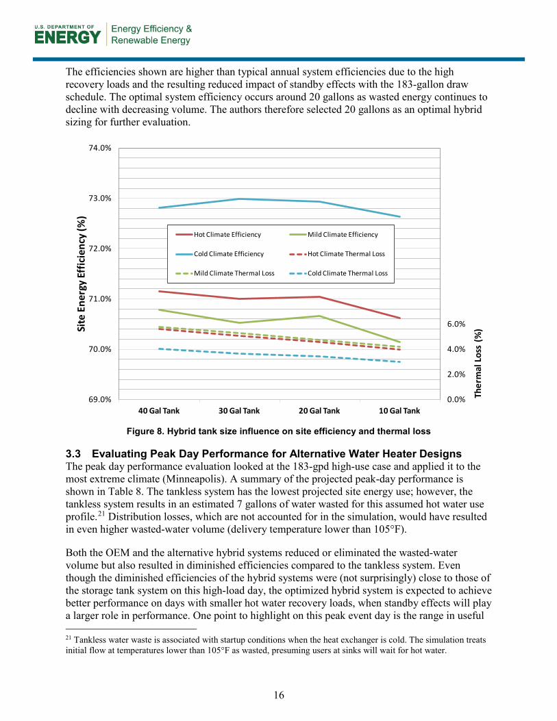
OEM Hybrid 0.66 n/a 3.2 Peak Day Performance Simulations To Determine Hybrid Tank Sizing The size of the storage tank in hybrid systems is best optimized for the specific climate and load; however, to evaluate a single hybrid system that would be appropriate for all climates, a series of simulations were conducted to find the best balance point for the three climate types. Figure 8 shows the results across the three climates for tank sizing options ranging from 40 gallons (consistent with OEM hybrid water heater), to a 10-gallon buffer tank. The systems were exercised with the 183 gallon design-load draw day and evaluated for site energy efficiency and thermal loss. The thermal loss term is calculated as the difference between the energy delivered from the tankless heat exchanger and the useful energy delivered by the storage tank, and therefore reflects storage losses and the delivered energy leaving the water heater that is lower than 105°F. The secondary Y-axis plots thermal loss as a percentage of the useful energy delivered by the storage tank.
16
The efficiencies shown are higher than typical annual system efficiencies due to the high recovery loads and the resulting reduced impact of standby effects with the 183-gallon draw schedule. The optimal system efficiency occurs around 20 gallons as wasted energy continues to decline with decreasing volume. The authors therefore selected 20 gallons as an optimal hybrid sizing for further evaluation.
Figure 8. Hybrid tank size influence on site efficiency and thermal loss
3.3 Evaluating Peak Day Performance for Alternative Water Heater Designs The peak day performance evaluation looked at the 183-gpd high-use case and applied it to the most extreme climate (Minneapolis). A summary of the projected peak-day performance is shown in Table 8. The tankless system has the lowest projected site energy use; however, the tankless system results in an estimated 7 gallons of water wasted for this assumed hot water use profile.21 Distribution losses, which are not accounted for in the simulation, would have resulted in even higher wasted-water volume (delivery temperature lower than 105°F).
Both the OEM and the alternative hybrid systems reduced or eliminated the wasted-water volume but also resulted in diminished efficiencies compared to the tankless system. Even though the diminished efficiencies of the hybrid systems were (not surprisingly) close to those of the storage tank system on this high-load day, the optimized hybrid system is expected to achieve better performance on days with smaller hot water recovery loads, when standby effects will play a larger role in performance. One point to highlight on this peak event day is the range in useful 21 Tankless water waste is associated with startup conditions when the heat exchanger is cold. The simulation treats initial flow at temperatures lower than 105°F as wasted, presuming users at sinks will wait for hot water.
0.0%
2.0%
4.0%
6.0%
8.0%
10.0%
12.0%
14.0%
16.0%
18.0%
20.0%
69.0%
70.0%
71.0%
72.0%
73.0%
74.0%
40 Gal Tank 30 Gal Tank 20 Gal Tank 10 Gal Tank
Ther
mal
Los
s (%
)Site
Ene
rgy
Effic
ienc
y (%
)
Hot Climate Efficiency Mild Climate Efficiency
Cold Climate Efficiency Hot Climate Thermal Loss
Mild Climate Thermal Loss Cold Climate Thermal Loss

17
hot water among the system types. The OEM hybrid is most effective at delivering a steady output temperature (due to its high capacity and large storage volume), followed by the conventional gas storage. The tankless and alternative hybrid deliver 2%–4% less “useful” energy.22
Table 9. Minneapolis Results for a High Consumption Day in February (183 gpd)
Water Heater Type Gas Storage
Tankless (175 kBtu)
OEM Hybrid (40 gal/91 kBtu)
Alternative Hybrid
(20 gal/75 kBtu) Gas Usage (therms/day) 1.82 1.61 1.87 1.73
Electric Usage (kWh/day) 0 0.22 0.63 0.55 Site Energy (Btu/day) 181,900 161,500 188,800 174,700
Useful Energy (Btu/day) 132,400 129,500 135,500 127,200 Daily Site Efficiency 73% 80% 72% 73%
Hot Water Gallons Wasted 0 7 0 1 3.4 Annual Performance Simulations The four water heaters (storage tank, tankless, OEM hybrid, and alternative hybrid) were next evaluated using the annual hot water draw profiles and the three representative climates. The alternative hybrid system was also run with two control strategies to see if performance improvements could be realized:
Increase the tankless water heater outlet set point to 160°F (denoted as “160 TWH”).
In addition to the 160°F set point, boost the storage tank set point (+10°F) during the winter season23 from 5–8 a.m. and 6–9 p.m. (denoted as “160 TWH + Boost”).
The annual water use profiles were derived from the Building America DHWESG (Hendron and Burch 2008) for one-bedroom (36 gpd), two-bedroom (57 gpd), and five-bedroom households (96 gpd). The average annual system efficiencies are tabulated in Table 9. Annual efficiencies are projected to increase with load, most significantly for the standard gas storage water heater. For the alternative hybrid, the “boost” function slightly degraded annual projected efficiencies because higher standby losses during the boost period offset any improvement in thermal energy delivered.
Table 10 and Table 11 provide a closer look at the one-bedroom and five-bedroom cases, including projected energy use, average daily useful energy, site efficiency, and gallons of water wasted. Even though the tankless system has the highest efficiency, it is projected to waste nearly 1,000 gallons of water per year. Not surprisingly, the alternative hybrid systems deliver within 1% of the annual energy output of the base gas storage water heater, in contrast to the 4% discrepancy on the peak day where the system is taxed by the extreme loads.
22 For the alternative hybrid, this degraded output is a function of the high hot water loads, which will be realized infrequently for most applications. 23 As determined by House Simulation Protocol climate-specific criteria for seasonal switchover

18
Table 10. Annual Projected System Efficiencies using DHWESG draw profiles for Minneapolis
System 1 Bedroom 36 GPD
2 Bedroom 56 GPD
5 Bedroom 62 GPD
Gas Storage 52.4% 59.0% 64.0% Gas Tankless 68.5% 71.0% 72.5% OEM Hybrid 55.7% 61.3% 64.6%
Alternative Hybrid 20 gal 57.6% 61.1% 64.1% Alternative Hybrid 20 gal, 160 TWH 57.3% 61.4% 64.5%
Alternative Hybrid 20 gal, 160 TWH + Boost 56.8% 61.1% 64.2%
Table 11. Annual Simulated Results for Minnesota One-Bedroom Case
Gas
Sto
rage
Tan
kles
s
OE
M
Hyb
rid
Alte
rnat
ive
Hyb
rid
Alte
rnat
ive
Hyb
rid
160
TW
H
Alte
rnat
ive
Hyb
rid
160
TW
H
+Boo
st
Annual Gas Use (therms/yr) 160 110 149 141 144 146
Annual Electric Use (kWh/yr) 0 51 91 82 58 60
Annual Site Energy (MBtu/yr) 16.05 11.21 15.18 14.42 14.59 14.76
Average Useful Energy (Btu/day) 23,000 21,000 23,200 22,700 22,900 23,000
System Site Efficiency 52% 68% 56% 58% 57% 57%
Hot Gallons Wasted (gal/yr and % of
total)
21 gal (0.2%)
986 (7.6%)
0 (0%)
121 (0.9%)
78 (0.6%)
60 (0.5%)
Figure 9 shows annual system site efficiencies for each water heater type under varying loads in the three climates investigated (Sacramento, Minneapolis, and Phoenix). The lower hot water use scenarios clearly demonstrate a larger spread in projected annual efficiencies. As the water use increases the efficiencies for all climates converge to 73% for the tankless system 63% for the hybrid systems, and 60%–63% for the storage tank systems. The hybrid systems show greater relative improvement in efficiency in mild and warm climates, especially in lower load homes; however, in cold climates with higher loads the relative efficiency improvement is reduced.

19
Figure 9. Annual system site efficiency as a function of hot water draw volume and climate
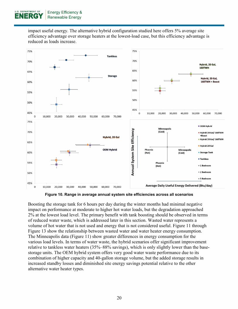
Figure 10 demonstrates how the load on the water heater is the primary factor that impacts the efficiency of the systems. The bottom right element in Figure 10 provides a key for understanding the results in the other three quadrants of the figure. Color coding of the symbol defines the system type, and the shape of the node defines the modeled hot water load (one-, three-, or five-bedroom home). To provide a clearer rendering of the results each quadrant contains a portion of the results. The top left includes the standard storage and gas tankless water heaters, the bottom left the OEM hybrid and alternative hybrid, and the top right looks at the impact of the alternative hybrid control options. The symbol is located at the average recovery load and efficiency from the three climates modeled. The vertical and horizontal lines denote the variation among the climates.
For each system type, as the hot water load increases, the projected efficiency increases as the overall impact of standby operation is reduced. This is most pronounced for the base storage water heater and least pronounced for the tankless water heater. The range in efficiencies between units also narrows with increasing load; the five-bedroom case has an efficiency improvement of slightly less than 10% over the base-case storage water heater, despite a significant range in useful energy delivered. The range in useful energy delivered varies significantly with higher-load homes across the studied climates. In addition to the change in hot water gallons/day, variations in entering cold water temperature and (to a lesser extent) the ability for the unit to meet the hot water loads that exceed the 105°F minimum temperature also
40%
45%
50%
55%
60%
65%
70%
75%
35 45 55 65 75 85 95
Annu
al Sy
stem
Site
Eff
icie
ncy
Hot Water Consumption (GPD)
Tankless, Mn Tankless, Sac Tankless, Phx
Hybrid, Mn Hybrid, Sac Hybrid, Phx
Storage Tank, Mn Storage Tank, Sac Storage Tank, Phx
20
impact useful energy. The alternative hybrid configuration studied here offers 5% average site efficiency advantage over storage heaters at the lowest-load case, but this efficiency advantage is reduced as loads increase.
Figure 10. Range in average annual system site efficiencies across all scenarios
Boosting the storage tank for 6 hours per day during the winter months had minimal negative impact on performance at moderate to higher hot water loads, but the degradation approached 2% at the lowest load level. The primary benefit with tank boosting should be observed in terms of reduced water waste, which is addressed later in this section. Wasted water represents a volume of hot water that is not used and energy that is not considered useful. Figure 11 through Figure 13 show the relationship between wasted water and water heater energy consumption. The Minneapolis data (Figure 11) show greater differences in energy consumption for the various load levels. In terms of water waste, the hybrid scenarios offer significant improvement relative to tankless water heaters (35%–88% savings), which is only slightly lower than the base-storage units. The OEM hybrid system offers very good water waste performance due to its combination of higher capacity and 40-gallon storage volume, but the added storage results in increased standby losses and diminished site energy savings potential relative to the other alternative water heater types.

21
In the warmer Phoenix and Sacramento climates, the projected water waste from the alternative hybrid system is nearly equal to that of the base storage water heater. Combined with a higher projected site efficiency, the 20-gallon storage hybrid unit with the higher (160°F) tankless set point is a valuable improvement option for the hybrid, resulting in a fraction of the water waste standalone tankless unit’s experience.
Figure 11. Comparison of Minneapolis annual site energy use to wasted water (gallons)
Figure 12. Comparison of Sacramento annual site energy use to wasted water (gallons)

22
Figure 13. Comparison of Phoenix annual site energy use to wasted water (gallons)
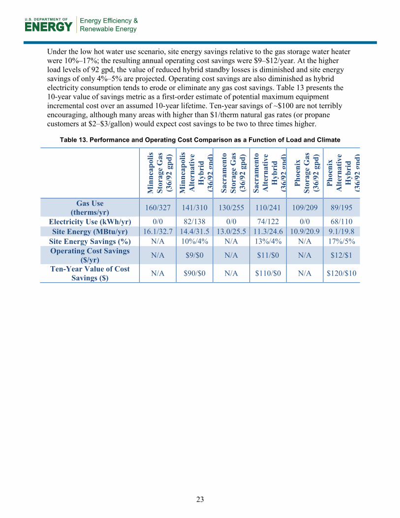
3.5 Preliminary Economic Assessment The performance projections presented in this study indicate significant variations in energy use, efficiency, and water waste characteristics among the various configurations modeled. Table 12 summarizes annual energy use and projected operating costs for the mainstream conventional gas storage water heater and the alternative hybrid configuration. The low- and high-load cases (36 and 92 gpd average use) are shown to highlight the variability in energy and cost impacts based on load. Operating costs were calculated using BEopt assumed national average rates of $1/therm and $0.1212/kWh.
Table 12. Annual Simulated Results for Minnesota Five-Bedroom Case
Gas
St
orag
e
Tan
kles
s
OE
M
Hyb
rid
Alte
rnat
ive
Hyb
rid
Alte
rnat
ive
Hyb
rid
160T
WH
Alte
rnat
ive
Hyb
rid
160
TW
H
+Boo
st
Annual Gas Use (therms/yr) 327 264 327 310 317 319 Annual Electricity Use
(kWh/yr) 0 59 155 138 95 98
Annual Site Energy (MBtu/yr) 32.67 26.64 33.28 31.49 3202 32.23
Average Useful Energy (Btu/day) 57,200 53,200 58,900 55,300 56,600 56,700
System Site Efficiency 64% 73% 65% 64% 64% 64% Hot Gallons Wasted (gal/yr
and % of total) 808 gal (2.4%)
2,705 (8.1%)
200 (0.6%)
1,749 (5.2%)
1,274 (3.8%)
1,217 (3.6%)
23
Under the low hot water use scenario, site energy savings relative to the gas storage water heater were 10%–17%; the resulting annual operating cost savings were $9–$12/year. At the higher load levels of 92 gpd, the value of reduced hybrid standby losses is diminished and site energy savings of only 4%–5% are projected. Operating cost savings are also diminished as hybrid electricity consumption tends to erode or eliminate any gas cost savings. Table 13 presents the 10-year value of savings metric as a first-order estimate of potential maximum equipment incremental cost over an assumed 10-year lifetime. Ten-year savings of ~$100 are not terribly encouraging, although many areas with higher than $1/therm natural gas rates (or propane customers at $2–$3/gallon) would expect cost savings to be two to three times higher.
Table 13. Performance and Operating Cost Comparison as a Function of Load and Climate
Min
neap
olis
St
orag
e G
as
(36/
92 g
pd)
Min
neap
olis
Alte
rnat
ive
Hyb
rid
(36/
92 g
pd)
Sacr
amen
to
Stor
age
Gas
(3
6/92
gpd
)
Sacr
amen
to
Alte
rnat
ive
Hyb
rid
(36/
92 g
pd)
Phoe
nix
Stor
age
Gas
(3
6/92
gpd
)
Phoe
nix
Alte
rnat
ive
Hyb
rid
(36/
92 g
pd)
Gas Use (therms/yr) 160/327 141/310 130/255 110/241 109/209 89/195
Electricity Use (kWh/yr) 0/0 82/138 0/0 74/122 0/0 68/110 Site Energy (MBtu/yr) 16.1/32.7 14.4/31.5 13.0/25.5 11.3/24.6 10.9/20.9 9.1/19.8
Site Energy Savings (%) N/A 10%/4% N/A 13%/4% N/A 17%/5% Operating Cost Savings
($/yr) N/A $9/$0 N/A $11/$0 N/A $12/$1
Ten-Year Value of Cost Savings ($) N/A $90/$0 N/A $110/$0 N/A $120/$10

24
4 Conclusions
The challenge in developing a retrofit gas water heater that does not require a change in gas line sizing or venting system is to achieve optimized operating efficiencies and limit the combustion efficiency to a level that will preclude the possibility of condensing flue gases.
This evaluation projects that average efficiency gains of 4% (and as high as 9%) were achievable with a 75,000 Btu/h input water heater with a 20-gallon storage tank. Performance of the hybrid system modeled is projected to be better as loads diminish due to either a warmer climate or lower hot water loads. This projection suggests that lower load applications in warm to hot climates would be a preferred market for the hybrid water heater modeled in this study.
The overall projected efficiency benefits identified in this study did not achieve the anticipated 71-73% projected efficiency levels targeted in the GTI HOT project. The HOT performance targets combined lab testing results with calculated expected benefits for various system improvements. Further lab and field evaluations are warranted to determine if improvements can raise annual in-situ operating efficiencies higher than 70%.
The primary research questions addressed include:
1. What storage volume sizing is needed to provide adequate performance with a 75-kBtu/h input limitation given realistic design day hot water loads in both mild and cold climates?
Simulation results suggest a 20-gallon storage tank is appropriate to balance performance and hot water delivery characteristics. This finding is consistent with results from the GTI HOT project. The projected site energy efficiency on a high-load design day (183 gpd) ranged from 70.6% in milder climates to slightly lower than 73% in cold climates. The thermal losses, which include tank storage loss and wasted water (<105°F delivery temperature), represent 3.4%–4.7% of the total site energy consumed.
2. How significant are performance variations with climate and hot water load?
Hybrid water heaters experience less variation in site efficiency across the three climates compared with standard atmospheric gas storage water heaters. This is primarily due to the smaller storage volume in the hybrid water heater and the elimination of the center flue. In cold climates, storage water heaters experience a 4%–7% increase in efficiency compared with hot climates; the optimized hybrid heater experiences a 0.5%–3% increase. In the lower load scenarios climate has more impact on total system site energy efficiency, because standby effects become more significant. Daily load levels, however, influence efficiency to a greater extent. Atmospheric storage gas water heaters are projected to provide a 12%–15% efficiency increase from the lowest to the highest load scenarios modeled; hybrid water heaters are projected to experience a 6%–9% increase. The significant decrease in storage water efficiency at low recovery loads is an important issue to consider in a future with zero energy homes and greater population growth in the southern United States.
Water use efficiency varies significantly with climate. In colder climates an average of 8.5 times more water is wasted by hybrid water heaters than in hot climates. In terms of hot water load, water waste can be 14.5 times higher in the high-load case (five-bedroom) than in the low-load

25
case (one bedroom) in cold climates. In hot climates the high-load case wastes only two times more than the low-load case. Although the water use impact is small from an economic perspective, water efficiency is becoming an increasingly important consideration in many parts of the country.
3. How does a hybrid gas water heater compare to a conventional gas storage water heater in providing adequate-quality hot water delivered under varying load conditions?
Modeling results suggest that the gas hybrid water heater (as modeled) may not deliver equal hot water performance relative to conventional gas storage water heaters. This is particularly true in the cold Minneapolis climate. In low-load Minneapolis conditions the hybrid is projected to waste as much as 5.7 times more water than the storage unit and to drop to 2.1 times under high-load conditions.24
In mild and warm climates hybrid water heaters are more favorable in providing quality hot water. Water waste can be as high as 1.5 times the base gas storage unit in high-use conditions and as low as 56% that of the storage in high-use conditions in hot climates.
4. What is the impact of control strategies, such as strategically overheating storage, on efficiency and hot water delivery?
In the OEM and standard alternative hybrid water heater scenarios, the delivery temperature of the tankless water heater was set 10°F higher than the storage tank set point. By increasing the set point of the tankless water heater to 160°F, the alternative hybrid unit was able to better meet minimum delivery temperatures and wasted on average 37%–400% less water than the base-case gas storage unit, depending on the load and climate. The minimal impact of the improved water use efficiency with this strategy was that the annual site energy efficiency dropped as much as 1% (average from 60.6% to 60%).
By changing the tank heating strategy to boost during specific times of the day, which preemptively met the expected high load periods of the day with more stored hot water, the water waste was reduced an additional 5%–30%; however, the site efficiency dropped as much as 2% (average reduction from 60.6% to 59.6%). Although the water waste benefit presumably translates into more satisfied occupants, this benefit must be weighed against the energy impacts. More complex adaptive control strategies may well provide better operating efficiencies and would warrant further evaluation if the concept advances.
24 To put these numbers into perspective, for the low-load case the added hot water waste is equal to about 10 showers annually (when assuming 10 gallons of hot water use per shower); the high-load case is equal to about 94 showers annually.

26
References
Aquacraft. 2008. Hot & Cold Water Data from EPA Retrofit Studies – EBMUD & Seattle. Boulder, CO: Aquacraft, Inc.
Burch, J., and Christensen, C. “Toward Development of an Algorithm for Mains Water Temperature,” American Solar Energy Society Annual Conference, 2007.
Glanville, P., Kalensky, D., and Kosar, D. Gas Technology Institute. 2009. Advanced Gas Appliance Development/Task 6 Hybrid Optimized Tankless Water Heating System. California Energy Commission, PIER Building End-Use Energy Efficiency Program. CEC-500-05-011.
Goetzler, W., Guernsey, M., and Droesch, M. 2014. Research & Development Roadmap for Emerging Water Heating Technologies. Prepared by Navigant Consulting, Inc. DOE/EE-1136. http://energy.gov/sites/prod/files/2014/09/f18/WH_Roadmap_Report_Final_2014-09-22.pdf.
Hendron, R., and Burch, J. 2008. Development of Standardized Hot Water Event Schedules for Residential Buildings. NREL/PR-550-40874. Presented at the 2008 Energy Sustainability Conference. http://www.nrel.gov/docs/fy08osti/40874.pdf.
Hoeschele, M., and Weitzel, E. 2013. “Monitored Performance of Advanced Gas Water Heaters in California Homes.” ASHRAE Transactions 119 (1):214–225.
KEMA. 2010. Residential New Construction (RNC) Programs Impact Evaluation Volume I California Investor‐Owned Utilities’ Residential New Construction Program Evaluation for Program Years 2006‐2008. http://www.calmac.org/publications/RNC_Final_Evaluation_Report.pdf.
Kosar, D., Glanville, P., and Vadnal, H. 2012. Residential Water Heating Program. California Energy Commission. Publication number: CEC-500-2013-060. http://www.energy.ca.gov/2013publications/CEC-500-2013-060/.
Lutz J.D., Renaldi, A.B. Lekov, Y.Q., and Moya, M. 2011. Hot Water Draw Patterns in Single-Family Houses: Findings from Field Studies. Lawrence Berkeley National Laboratory, PIER Buildings End-Use Energy Efficiency. LBNL-4830E.
Mayer, P., and DeOreo, W. 1999. Residential End Uses of Water, Prepared for the American Water Works Association, Boulder, CO: Aquacraft, Inc.
Parker, M. 2011. “American Water Heating Dynamics: Present and Future.” Presented at A.O. Smith.
TESS. 2010. Type 534: Vertically Cylindrical Storage Tank with Immersed Heat Exchanger. TRNSYS v. 17.01software documentation. Released January 1, 2011. Madison, WI. Thermal Energy System Specialists, LLC.
Schoenbauer, B., Hewett, M., and Bohac, D. 2011. “Actual Savings and Performance of Natural Gas Instantaneous Water Heaters.” ASHRAE Transactions 117 (1):657–672.

27
Appendix A: Storage Type 534 and Tankless Type 940 Water Heater Model Descriptions
(Model descriptions provided courtesy of Thermal Energy System Specialists, LLC)
28
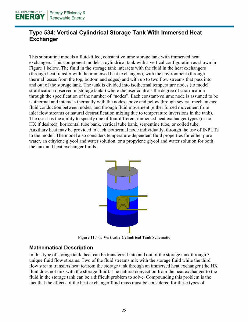
Type 534: Vertical Cylindrical Storage Tank With Immersed Heat Exchanger
This subroutine models a fluid-filled, constant volume storage tank with immersed heat exchangers. This component models a cylindrical tank with a vertical configuration as shown in Figure 1 below. The fluid in the storage tank interacts with the fluid in the heat exchangers (through heat transfer with the immersed heat exchangers), with the environment (through thermal losses from the top, bottom and edges) and with up to two flow streams that pass into and out of the storage tank. The tank is divided into isothermal temperature nodes (to model stratification observed in storage tanks) where the user controls the degree of stratification through the specification of the number of “nodes”. Each constant-volume node is assumed to be isothermal and interacts thermally with the nodes above and below through several mechanisms; fluid conduction between nodes, and through fluid movement (either forced movement from inlet flow streams or natural destratification mixing due to temperature inversions in the tank). The user has the ability to specify one of four different immersed heat exchanger types (or no HX if desired); horizontal tube bank, vertical tube bank, serpentine tube, or coiled tube. Auxiliary heat may be provided to each isothermal node individually, through the use of INPUTs to the model. The model also considers temperature-dependent fluid properties for either pure water, an ethylene glycol and water solution, or a propylene glycol and water solution for both the tank and heat exchanger fluids.
Figure 11.4-1: Vertically Cylindrical Tank Schematic
Mathematical Description In this type of storage tank, heat can be transferred into and out of the storage tank through 3 unique fluid flow streams. Two of the fluid streams mix with the storage fluid while the third flow stream transfers heat to/from the storage tank through an immersed heat exchanger (the HX fluid does not mix with the storage fluid). The natural convection from the heat exchanger to the fluid in the storage tank can be a difficult problem to solve. Compounding this problem is the fact that the effects of the heat exchanger fluid mass must be considered for these types of

29
systems. The problem breaks down into the required solution of two coupled differential equations:
dTTank/dt = (Qin,Tank - Qout,Tank)/CTank
Eq. 11.4-1 dTHX/dt = (Qin,HX - Qout,HX)/CHX
Eq. 11.4-2 where Qin,Tank and Qout,Tank are functions of the ambient temperature, the inlet fluid conditions and flow rates, and the heat exchanger temperature, and Qin,HX and Qout,HX are functions of the inlet fluid temperature and flow rate to the heat exchanger and the tank temperatures. While there are other available methods to solve coupled differential equations, we decided to solve the problem with an approximate analytical solution. The analytical solution has several inherent advantages over numerical solutions. First, the subroutine solves its own mathematical problem and does not have to rely on non-standard numerical recipes that must be attached to the subroutine. In this way, the subroutine can be imported into any FORTRAN compiler without problems. Secondly, some of the other solution methods (mainly the numerical solutions) are extremely dependent on the simulation timestep and may not converge under certain circumstances commonly encountered in domestic hot water systems (namely high flow rates for example). The analytical solution is timestep independent but does require an iterative solution inside the subroutine to solve the coupled differential equations. While solving two coupled differential equations iteratively can sometimes lead to convergence problems, this does not seem to be the case with this model under almost all operating scenarios.
To solve the differential equations analytically, the equations are placed into the form:
dT/dt = aT+b
Eq. 11.4-3 Where T is the dependent variable, it is time, a is a constant and b may be a function of time or the dependent variable. If b is a constant, than the solution of this differential equation can be readily solved. If b is not constant, then a reasonable approximation to the analytical solution can be found by assuming that b is constant over the timestep and equal to its average value over the timestep.
At any time (for a not equal to zero):
Tfinal = (Tinitial + bave/a) * e(a t) - bave/a
Eq. 11.4-4 where: bave = b(Tave)
Eq. 11.4-5 and: Tave = 1/a t*(Tinitial + bave/a) * (e(a t) - 1) - bave/a
Eq. 11.4-6

30
With this assumption, the problem becomes straightforward to solve. Simply write the differential equation in the correct form, determine a and bave and solve for Tfinal and Tave. Then recalculate bave and iterate until the temperatures converge.
While the assumption that b is constant over the timestep (and equal to its average value) is not technically correct (b for the tank is a function of the heat exchanger temperature for example), it is a reasonable approximation for the small timesteps we are using in the TRNSYS simulation (maximum timestep=1 hour).
This subroutine allows the user to designate the level of stratification for the storage tank by specifying a number of tank nodes (N). The tank is then divided into N horizontal nodes of equal volume (before the placement of the heat exchanger which reduces the volume (and hence the capacitance) of the node). Each of the tank nodes is assumed to be isothermal. Node 1 is assumed to be at the top of the storage tank. The greater the number of nodes, the greater the stratification in the storage tank. Unreasonably increasing the number of nodes may slow down the simulation dramatically.
The heat exchangers are also divided into a user-defined number of isothermal nodes (Nhx), but these nodes are arranged along the flow direction of the heat exchanger (along the length of the pipe). Adjacent heat exchanger nodes interact thermally only via the flow stream, conduction is not considered between heat exchanger nodes.
For horizontal tube bank heat exchangers, each tube comprising the heat exchanger is uniformly divided into Nhx nodes along the horizontal direction. The user must supply the fraction of the total number of heat exchanger pipes that lie completely within each of the tank nodes.
Figure 11.4-2: Horizontal Tube Bank HX
For vertical tube bank heat exchangers, the tubes comprising the heat exchanger are divided into Nhx nodes along the vertical direction. For each heat exchanger node, the user must supply the fraction of the heat exchanger pipe length to be assigned to that node and the tank node in which this heat exchanger node is completely located. It is possible to have more than one heat exchanger node located within a tank node.

31
Figure 11.4-3: Vertical Tube Bank HX
For coiled tube heat exchangers, the tubes comprising the heat exchanger (there may be more than one tube bundled together) are divided into Nhx nodes along the flow direction. For each heat exchanger node, the user must supply the fraction of the heat exchanger pipe length to be assigned to that node and the tank node in which this heat exchanger node is completely located. It is possible to have more than one heat exchanger node located within a tank node.
Figure 11.4-4: Coiled Tube HX
For serpentine tube heat exchangers, the tubes comprising the heat exchanger (there may be more than one tube bundled together) are divided into Nhx nodes along the flow direction. For each heat exchanger node, the user must supply the fraction of the heat exchanger pipe length to be assigned to that node and the tank node in which this heat exchanger node is completely located. It is possible to have more than one heat exchanger node located within a tank node. With the serpentine tube HX, complex flow patterns through the tank may be specified and studied.
Figure 11.4-5: Serpentine Tube HX
32
Heat Exchanger: This model allows the user to designate which of 4 unique heat exchanger arrangements are immersed in the storage tank.
vertical tube bank
horizontal tube bank
serpentine tube
coiled tube The outlet temperature at any time during the simulation for the heat exchanger flow stream is the average temperature of the heat exchanger node that contains the outlet (the last specified node) over the timestep. Header volumes (a user-supplied parameter) are added to the first and last heat exchanger nodes. The heat exchanger and storage tank interact thermally through natural convection heat transfer from the heat exchanger outer surface to the tank fluid (or in this case from the outer surface of the heat exchanger node to the tank fluid node). The overall heat transfer coefficient (UA) of the heat exchanger to tank heat transfer for any heat exchanger node can be expressed as:
n/UA =(1/hoAo) + Rw +(1/hiAi)
Eq. 11.4-7 where: n = number of identical tubes (pipes) ho = outer surface heat transfer coefficient (tank fluid side) Ao = outer surface area of the HX node Rw = tube wall resistance hi = inner surface heat transfer coefficient (in the tubes) ai = inner surface area of the HX node and: ho = Nud * k/do
Eq. 11.4-8 where: Nud = Nusselt number based on tube diameter k = fluid thermal conductivity do = outer pipe diameter and: Nud = C * (Ra)n * (GF)m
Eq. 11.4-9 where: Ra = Rayleigh number for the tank fluid (based on fluid properties at (Tsurf + T )/2 this requires an iterative solution as Tsurf depends on the heat transfer) Tsurf = outer surface temperature of HX

33
T = temperature of the tank node containing this HX node C, n, GF, and m = user supplied parameters and: Rw = ln(ro/ri)/(2 Lpipekw)
Eq. 11.4-10 where: ro = outer pipe radius ri = inner pipe radius Lpipe = length of pipe node kw = HX wall thermal conductivity The inner surface heat transfer coefficient (hi) is dependent on the type of heat exchanger as well as the fluid properties. The flow is assumed to be fully developed and the internal convection coefficient is based on the length of the tubes; and not on the length of the node. For all cases the Reynolds number (Rehx) and Prandtl number (Prhx) are calculated as:
Rehx = 4 m / ( di )
Eq. 11.4-11 Prhx = Cp * / k
Eq. 11.4-12 where: m = Flow rate through 1 tube of the HX di = inner tube diameter
= fluid viscosity k = fluid thermal conductivity Cp = fluid specific heat For all heat exchanger types with the exception of the coiled tube HX, the transition from laminar flow to turbulent flow occurs at a Reynolds number of 2300. For coiled tube heat exchangers, the critical Reynolds number for transition from laminar flow to turbulent flow is calculated as:
Recrit=20000*(di/dcoil)0.32
Eq. 11.4-13 where: dcoil = diameter of the coiled tube heat exchanger For coiled tube heat exchangers the Nusselt number correlation for laminar flow is:
Eq. 11.4-14
Nusselthx = 4811
+
5111
1 +
1342Prhx
HE2
2
3
+ 1.816 · HE
1 + 1.15Prhx
1.5
(1 / 3 )

34
where:
Eq. 11.4-15
and for turbulent flow conditions is:
Eq. 11.4-16
For serpentine heat exchangers, vertical tube bank heat exchangers and horizontal tube bank heat exchangers the Nusselt number correlation for laminar flow conditions is: For cases where: Ltube / di 0.0425 * Rehx * Prhx
Eq. 11.4-17
otherwise:
Eq. 11.4-18
and for turbulent flow conditions is:
( Prhx 1.5 )
Eq. 11.4-19
( Prhx > 1.5 )
Eq. 11.4-20
The internal heat transfer coefficient is then: hi = Nusselthx * k /di
Eq. 11.4-21 For cases where there is no flow through the heat exchanger, the Nusselt number is set to 1.0 for the calculation of the internal heat transfer coefficient. Finally, the heat transfer between the tank node (j) and heat exchanger node (k) can be calculated as: Qhx,j k = UAj,k * (Ttank,j - Thx,k)
Eq. 11.4-22
The other component of heat transfer for the heat exchanger node (besides the heat transfer to the storage tank fluid) is via fluid flow through the heat exchanger: Qflow = m * Cp * (Thx,k - Tin)
Eq. 11.4-23
HE = Rehx ·
didcoil
0.5
1 + Pitchcoil
· di
2
Nusselthx = 0.023 · Rehx0.85 · Prhx
0.4 · di
dcoil
0.1
Nusselthx = 3.663 + 1.613 · Rehx · Prhx · di
L tube
(1 / 3 )
Nusselthx = 4.364
Nusselthx = 0.0214 · (Rehx0.8 – 100) · Prhx
0.4
Nusselthx = 0.012 · (Rehx0.87 – 280) · Prhx
0.4

35
where: m = mass flow rate through the node (depends on HX flow rate and the number of tubes) Cp = fluid specific heat Tin = the inlet temperature to the heat exchanger node (this temperature may be the entering HX temperature or the temperature of the node upstream of this node depending on the location of the node) Thx,k = the temperature of the heat exchanger node The a and b terms for the differential equation (dT/dt = aT + b) for the heat exchanger heat transfer for the node can be expressed as: ahx,k = ( m * Cp - UAj,k ) / Capk
Eq. 11.4-24 bhx,k = [(- m * Cp * Tin) + (UAj,k * Ttank,j ) ] / Capk
Eq. 11.4-25 where: Capk = mass of fluid in HX node * specific heat of HX fluid
Storage Tank: The storage tank model accounts for the following component heat transfers:
thermal losses to the environment through the top of the storage tank
thermal losses to the environment through the sides of the storage tank
thermal losses to the environment through the bottom of the storage tank
thermal losses to the environment through a gas flue passing through the tank
heat exchange with flowing and stagnant fluid in the heat exchanger
conduction between adjacent tank nodes
mixing between nodes to eliminate thermal instabilities
mixing between nodes due to load flow through the storage tank
auxiliary heat input to the tank
miscellaneous heat gains/losses to/from the tank
Top, Edge and Bottom Losses: The storage tank interacts thermally with its environment through heat losses (or gains) to the tank from the top, edges and bottom areas of the storage tank. The model allows the user to specify unique environment temperatures for the top surface, bottom surface and edges in order to increase the flexibility of the model. The heat transfer from the top, edges and the bottom of the storage for tank node j is:

36
Qloss,top,j = (Atop,j * Utop) * (Ttank,j - Tenv,top)
Eq. 11.4-26 Qloss,bottom,j = (Abottom,j * Ubottom) * (Ttank,j - Tenv,bottom)
Eq. 11.4-27 Qloss,edges,j = (Aedges,j * Uedges) * (Ttank,j - Tenv,edge)
Eq. 11.4-28 where: Atop,j = tank top surface area for thermal losses (all attributed to tank node 1) Abottom,j = tank bottom surface area for thermal losses (all attributed to tank node N) Aedge,j = tank top surface area for thermal losses (distributed equally amongst all the nodes) Utop = storage tank top heat loss coefficient Ubottom = storage tank bottom heat loss coefficient Uedge = storage tank edge heat loss coefficient Ttank,j = temperature of the tank node Tenv,top = tank environment temperature for losses through the top of the storage Tenv,bottom = tank environment temperature for losses through the bottom of the storage Tenv,top = tank environment temperature for losses through the edges of the storage
Gas Flue Losses: The storage tank also interacts thermally with its environment through heat losses from a gas flue which passes through the storage volume. The user specifies the overall heat loss coefficient from the tank node to the gas flue as parameter and provides the temperature of the gas flue as as INPUT to the model. The losses from the gas flue are set to zero if auxiliary energy is being added to the tank. The heat transfer from the storage to the gas flue for tank node j is:
Qloss,flue,j = UAflue,j * (Ttank,j – Tflue) * (1 – aux)
Eq. 11.4-29 where: UAflue,j = overall heat loss coefficient from node j to the gas flue Ttank,j = temperature of the tank node Tflue = the temperature of the gas flue (an INPUT)
aux = on/off indicator for whether auxiliary heat is being added to the storage tank
Conduction Effects: The nodes in the storage tank of this model can interact thermally via conduction between nodes. An additional term must be supplied by the user to account for conduction in the storage tank wall (and maybe even to account conduction in the heat exchanger wall). Conduction between nodes can be turned off by the user by setting the additional conductivity term (a parameter) less than zero. The formulation of the conductivity heat transfer from tank node j is:
Qcond,j = kj* Aj * (Tj – Tj+1) / Lcond,j + kj-1 * Aj-1 * (Tj – Tj-1) / Lcond,j-1
Eq. 11.4-30 Tj = temperature of this node Tj+1 = temperature of the node directly below the current node Tj-1 = temperature of the node directly above the current node

37
kj = thermal conductivity of fluid in node j (evaluated at average temperature between this node and the node below) kj-1 = thermal conductivity of fluid in node j (evaluated at average temperature between this node and the node above) Aj = conduction interface area between this node and the one below it (may be reduced by the presence of a heat exchanger tube passing through the boundary between the tank nodes) Aj-1 = conduction interface area between this node and the one above it (may be reduced by the presence of a heat exchanger tube passing through the boundary between the tank nodes) Lcond,j = vertical distance between the centroid of this node and the centroid of the node below Lcond,j-1 = vertical distance between the centroid of this node and the centroid of the node above
Inlet Flow Effects: This model allows the user to have multiple flow streams which pass into and out of the storage tank. There are several methods which dictate where the entering water is placed in the storage tank.
Fixed Inlets and Outlets (“Inlet Flow Mode” = 1): The user must specify the inlet and outlet locations (nodes) for each of the inlet and outlet streams. The temperatures at the outlets at any time are simply the average temperatures of the nodes containing the outlets over the simulation timestep. The user provides the inlet temperature and flow rate through each of the inlets. The inlet and outlet locations are also fixed throughout the simulation – they cannot be changed. The outlet flow rate from any outlet is simply the inlet flow rate from its paired inlet (for example 100 kg/h into inlet 1 causes 100 kg/h to exit the tank through outlet 1). An example is shown below of the path of the flow streams with the following conditions:
Stream 1 = 200 kg/h with Inlet in Node 4 and Outlet in Node 1
Stream 2 = 75 kg/h with Inlet in Node 1 and Outlet in Node 3

38
Figure 11.4-6: Example Flows
In this tank model, the inlet fluid into a node is completely mixed with the storage tank fluid at every timestep before this fluid moves on to the next node (the fluid flow path is directly from the inlet node to the outlet mode). For example, water at 10 C and at a flow rate of 200 kg/h enters node 4 (outlet = node 1) of a storage tank which has an initial temperature of 30 C. The 10 C inlet flow stream mixes with the 30 C water in the tank node causing the tank node to fall to 25 C (for example). 200 kg/h of 25 C water then crosses the boundary into node 3 where it mixes with the fluid in this boundary before moving on towards node 2 and eventually out through the outlet in node 1.
As mentioned earlier, each inlet to the tank is assumed to be paired with an outlet from the tank. In other words, you cannot have two outlets from the tank and only one inlet into the tank or two inlets to the tank and only one outlet from the tank. However, by the use of a Type 11 mixing valve (2 inlets 1 outlet) or a Type 11 flow diverter (1 inlet 2 outlets) in combination with this tank model you can effectively simulate these odd paired systems. For example, if you wished to simulate 100 kg/h of water entering the bottom of the storage tank (node 5) through an inlet port and 100 kg/h of water entering the middle of the tank (node 3) from a different fluid stream with 200 kg/h leaving through the top of the tank (node 1) in one outlet you could specify the following parameters:
“Inlet Flow Mode” = 1 Indicates the user will specify the inlet and outlet locations “Entry node for Inlet 1” = 5 Indicates the first inlet location is at the bottom of the tank “Exit node for Outlet 1” = 1 Indicates the first outlet location is at the top of the tank “Entry node for Inlet 2” = 3 Indicates the second inlet location is at the middle of the
tank “Exit node for Outlet 2” = 1 Indicates the second outlet location is at the top of the tank A Type 11 flow mixer is then used to mix the two outlet streams from the tank (they are both at the same temperature) and you have now effectively modeled a two inlet, 1 outlet storage tank.

39
Fractional Inlets with Fixed Outlets (“Inlet Flow Mode” = 2): The user must specify the outlet locations (nodes) for each of the streams. The temperatures at the outlets at any time are simply the average temperatures of the nodes containing the outlets over the simulation timestep. The user provides the inlet temperature and flow rate through each of the inlets. The inlet and outlet locations are also fixed throughout the simulation – they cannot be changed. The outlet flow rate from any outlet is simply the inlet flow rate from its paired inlet (for example 100 kg/h into inlet 1 causes 100 kg/h to exit the tank through outlet 1). The user also has the ability in this model to dictate which tank nodes receive the inlet fluid flow. This feature is useful to simulate cases where some of the inlet flow is not completely mixed within a node before moving on to the next node. For example, in high flow rate inlets, some of the inlet fluid may effectively “jet” past the inlet node and into several nodes beyond the inlet node. For this inlet fluid mode, the user must specify the fraction of unmixed inlet flow rate that ends up in each of the tank nodes as parameters to the model. For example let us consider the case where 1000 kg/h of cold mains water enters a warm storage tank (5 nodes) with high enough velocity to cause some of the fluid to “jet” into the two nodes above (nodes 4 and 3). Let us assume that 50% of the inlet fluid enters the bottom node and mixes with the fluid in that node and 35% of the inlet fluid mixes with the fluid in the node above the inlet node, and the remaining 15% of the inlet fluid mixes with the node 2 above the inlet (node 3). If the outlet from the tank is in node 2 we have the following flow pattern established for the model:
Figure 11.4-7: Fractional inlets with fixed outlets
Temperature Seeking Inlets with Fixed Outlets (“Inlet Flow Mode” = 3): The user must specify the outlet locations (nodes) for each of the streams. The temperatures at the outlets at any time are simply the average temperatures of the nodes containing the outlets over the simulation timestep. The user provides the inlet temperature and flow rate through each of the inlets. The inlet locations are then found by finding the tank node closest in temperature to

40
the inlet temperature and directing the entire inlet flow stream into this tank node. The outlet flow rate from any outlet is simply the inlet flow rate from its paired inlet (for example 100 kg/h into inlet 1 causes 100 kg/h to exit the tank through outlet 1). In this model, the inlet fluid into a node is completely mixed with the storage tank fluid at every timestep before this fluid moves on to the next node (the fluid flow path is directly from the inlet node to the outlet mode). For example, water at 10 C and at a flow rate of 200 kg/h enters node 4 (outlet = node 1) of a storage tank which has an initial temperature of 30 C. The 10 C inlet flow stream mixes with the 30 C water in the tank node causing the tank node to fall to 25 C (for example). 200 kg/h of 25 C water then crosses the boundary into node 3 where it mixes with the fluid in this boundary before moving on towards node 2 and eventually out through the outlet in node 1. This inlet flow mode is very similar to the first inlet mode except the inlet location is not specified by the user but rather found from the corresponding temperatures.
The heat transfer due to flow into a tank node is then expressed as:
Qflow,i,j = m in*fracin,j * Cp * Tin + m in,j-1 * Cp * Tj-1+ m in,j+1 * Cp * Tj+1 - m push * Cp * Tj
Eq. 11.4-31
where: m in = inlet mass flow rate into the tank m in,j-1 = mass flow rate of fluid into node from node above m in,j+1 = mass flow rate of fluid into node from node below fracin,j = fraction of inlet fluid flow that enters this tank node Cp = specific heat of the fluid Tin = the temperature of the inlet fluid entering the storage tank Tj = temperature of the tank node Tj-1 = the temperature of the tank node above the current node Tj+1 = the temperature of the tank node below the current node
Mixing Effects: At times, the nodes in the storage tank may become thermally unstable (a node has a higher temperature than the node above). If this happens, the model allows the user to "mix" the unstable nodes at a user-defined rate. While many of the tank models allow this instability mixing, most of the models calculate the effects using a simplifying assumption that speeds up the calculations but introduces some energy balance problems. The two most common tank models in TRNSYS calculate the temperatures of the nodes, then completely mix any nodes that are unstable at the end of the timestep to avoid problems. While this "averaging" of the tank temperatures (and hence an infinite flow mix between the nodes) is not a bad assumption, the energy balance is not correct as the tank losses, and other heat flows, are calculated with the tank temperatures before the mixing takes place. This model allows the user to utilize this method of mixing by specifying a negative value for the mixing flow rate input.
This model also allows the user a second method of calculating the mixing effect. In the second method the model calculates the elapsed time into the current timestep at which adjacent tank nodes would become unstable and then starts to mix the nodes at a user-defined flow rate until the nodes stabilize. In this manner (as separate differential equations for each unique mixing
41
period are calculated by the model), the overall energy balance is calculated correctly. Once two nodes begin to mix, they keep mixing until the temperatures stabilize or until the end of the current timestep; whichever occurs later.
The formulation of the mixing heat transfer between nodes is:
Qmix,j = m j * Cpj * (Tj – Tj+1) + m j-1 * Cpj-1 * (Tj – Tj-1)
Eq. 11.4-32 where m j = mixing flow rate between this node and the one below m j-1 = mixing flow rate between this node and the one above Cpj = average specific heat of fluid between this node and the one below Cpj-1 = average specific heat of fluid between this node and the one above Tj = temperature of current node Tj+1 = temperature of node below current node Tj-1 = temperature of node above current node Care should be taken when specifying large mixing flows between nodes as small temperature differences between node calculation iterations can lead to relatively large energy balance errors. The model reports the energy balance closure at each timestep so the user should check the results upon changing the mixing flow rate.
Auxiliary Heating Effects: This storage tank relies on external controls to add (or possibly remove) heat from the storage tank. This feature can be used to model auxiliary heating effects (electrical element, combustion heating, etc.). The user supplies heat input rates for each of the nodes in the storage tank through INPUTs to the model. For example, an aquastat model may sense the top node temperature of the storage tank and send a control signal to an auxiliary heater model that adds heat to the bottom node of the storage tank until the top node reaches its setpoint; at which time the control signal from the aquastat is disabled and input energy to the tank is ceased.
Miscellaneous Heat Inputs/Losses: This model allows the user to specify the magnitude and location of miscellaneous heat flows into (positive value) and out of the storage tank. This feature was added to account for things such as a pilot light in a gas storage tank or other unaccounted for gains or losses.
Solving the Tank Equations
The differential equations for the tank nodes can be written as: dTTank,j/dt = (Qin,Tank,j - Qout,Tank,j)/CTank,j
Eq. 11.4-33 or expanded to: dTTank,j/dt = (Qaux,j-Qhx,j k-Qloss,top,j-Qloss,bottom,j -Qloss,edges,j-Qcond,j-Qflow,i,j-Qmix,j) / CTank,j
Eq. 11.4-34

42
These equations are then placed in the form:
dT/dt = aT+b
Eq. 11.4-35 and a and b values are found for each node. The b term holds the temperatures of other tank nodes and heat exchanger nodes. These temperatures in the b term are assumed to be constant for the solution of the nodal differential equations at their average value over the timestep. The nodal differential equation is then solved (as described earlier), new final and average nodal temperatures are calculated and the entire process is repeated until a converged solution is obtained. Then the heat exchanger nodal calculations are repeated until all tank and heat exchanger nodes are converged.
As described earlier, mixing may initiate during the timestep if temperature inversions are observed between adjacent nodes. If a temperature inversion occurs, the time into the timestep at which the nodal temperatures become unstable is calculated. The results at this point are stored and a new solution is calculated with mixing occurring between the two offending nodes. Temperature inversions are again checked and a new time at which inversions occur may be found. This process is repeated until no new temperature inversions are calculated at which time the results from the model are reported. As in all TRNSYS components, the OUTPUTs from the model are assumed to be average values over the timestep.

43
TYPE 940: TANKLESS WATER HEATER
Image from http://www.plumbingsupply.com/infinion.html
General Description Type940 models a tankless water heater; a device used to heat a liquid stream by the addition of heat from either an electric heating element or a gas combustion heating source. In simple terms it is an auxiliary heater with internal controls to modulate the heat input to the fluid.
Nomenclature
[-] heating efficiency expressed as a fraction [-] control signal indicating fraction of capacity
A [m2] surface area for thermal losses
Cap [kJ/K] thermal capacitance of the device including the mass of water contained within the device
Cp [kJ/kg.K] specific heat
m [kg/hr] mass flow rate
P [kJ/hr] power
Q [kJ/hr] heat transfer rate
t [hours] time
T [C] temperature
U [kJ/hr.m2.K] heat transfer coefficient between the device and the surrounding air
Subscripts
average refers to the average conditions over the time interval or time period
delivered refers to the energy delivered to the flow stream passing through the device
final refers to the condition at the end of the timestep or time period
fluid refers to the fluid flowing through the device (typically water)

44
heat refers to the conditions in which the device is actively heating the fluid
i refers to a period of time during the current timestep
in refers to the condition at the inlet to the device
initial refers to the conditions at the beginning of the timestep or time period
period refers to a section of time during a timestep
pilot refers to the pilot light during periods in which the device is not actively heating the fluid
out refers to the condition at the outlet from the device
rated refers to the rated (maximum) condition
skin refers to the energy transferred from the device to the surroundings
stored refers to the change in energy of the fluid due to a change in temperature
surroundings refers to the conditions in which the device is located
timestep refers to the TRNSYS timestep for the simulation
Detailed Description
This component relies on a single differential equation to model the performance of the tankless water heater:
gssurroundinfluid
influidfluidfluidfluidpilotpilotratedheatfluid
TTUA
TTCpmQQdt
dTCap , (Eq. 940.1)
With this assumption, the temperature of the device at any time can be quickly calculated based on the current operating scenario. The temperature of the fluid exiting the device is assumed to be at the temperature of the entire device. In other words the temperature of the water in the device and the temperature of the enclosure are “lumped” together.
To solve the differential equations analytically, the equations are placed into the form:
bTadt
dTfluid
fluid (Eq. 940.2)
where T is the dependent variable, t is time, a is a constant and b may be a function of time or the dependent variable. If b is a constant, than the solution of this differential equation can be readily solved. If b is not constant, then a reasonable approximation to the analytical solution can be found by assuming that b is constant over the timestep and equal to its average value over the timestep.
At any time (for a not equal to zero):
abe
abTT ta
initialfinal (Eq. 940.3)
where
45
averageTbb (Eq. 940.4) and
abe
abT
taT ta
initialaverage 11 (Eq. 940.5)
With this assumption, the problem becomes straightforward to solve. Simply write the differential equation in the correct form, determine a and b for the current operating scenario and solve for Tfinal and Taverage. If required, then recalculate b and iterate until convergence is reached. In the current version of this component, b is a constant and no iterations are required. If the efficiency or loss coefficient were reworked to be a function of the fluid temperature for example, then iteration would be required.
One of the important features of tankless water heaters are their quick response to changing conditions. To study systems with quick response, small timesteps are typically used in TRNSYS. However, small timesteps substantially increase the simulation speed and running at timesteps approaching one second may not be feasible for annual simulations. Unfortunately large timesteps (15 minutes or greater) may cause severe over or under-heating of the fluid; as control decisions are then only made once each timestep.
To alleviate this problem, the model utilizes an internal control methodology that allows multiple control decisions to be made within a single timestep; possibly turning on and off the heating many times within a single timestep. The duration of each of these sub-timesteps is then recorded (along with the temperatures during each period) and the model reports the average conditions over the timestep (the standard TRNSYS output convention).
The device is “off” for the timestep if the inlet flow rate is zero or below the minimum flow rate for operation (a parameter). Whenever the device is off, energy is added to the fluid by the pilot light ( pilotpilot Q ), but the main heating control is off ( =0).
The model is also equipped with a “time delay” feature. If the conditions are such that the device was off due to a low-flow condition, and should now turn on, a user-specified amount of time must pass (a parameter) before the heating source is activated. During this period, the main heating source is off and the pilot light is activated.
The control logic for the model is illustrated below. It should be noted that if the capacity modulation algorithm finds a desired modulation below the minimum capacity fraction (a parameter), the device is turned off for that period and the temperatures are allowed to float until they cross the control boundaries.
The model also allows the user to specify the electrical energy consumed during standby operation and during active heating operation. This electrical energy does not influence the temperature of the fluid.

46
Was the device ON at the previous timestep?
Is the flow rate greater than the minimum flow
rate?
Is the flow rate greater than the minimum flow
rate?
N
The device is off for the remainder of the
timestep. Calculate the outlet temp. and exit.
N
Is the starting temperature less than the
setpoint - deadband?
Yes
No Leave or turn the device off (y=0) and go to OFF section.
Yes
Yes
N
Turn on the device at full capacity (y=1) and go to ON section.
Is the starting temperature less than the
setpoint – deadband?
Turn on the device at full capacity (y=1) and go to ON section.
Yes
No
Is the starting temperature less than the
setpoint?
Leave the device on and at its current capacity and go to ON section.
Yes
No
Is the starting temperature less than the
setpoint?
Yes
N
Modulate the capacity such that the setpoint temperature is maintained by finding the closest setting above the required capacity.
Yes

47
Calculate the outlet temperature at the end of
the timestep at the current capacity (y).
N
Leave the device on at full capacity (y=1) for the rest of the timestep and calculate the temps.
Is the final temp. < setpoint but > setpoint – deadband and do we have stepped control?
Is the device on at full capacity and the final temperature below the setpoint?
Yes
ON Section
Leave the device on at current capacity (y) for the rest of the timestep and calculate the temps.
Yes Exit the model
N
Is the final temp. < setpoint – deadband temperature?
Calculate the time required for the device to float down to the setpoint – deadband temperature.
Modulate the capacity such that the setpoint temperature is maintained (perfect) or find the closest setting below the required capacity (stepped) and restart the ON Section
Yes
N
Is the final temp. > setpoint temperature?
Calculate the time required for the device to float down to the setpoint temperature.
Yes
N
Does the device have perfect modulation?
Modulate the capacity such that the setpoint temperature is maintained Yes
N
Calculate the time for the device to float down to the setpoint minus deadband temperature.
Does the float time exceed the remainder of the timestep?
Finish the timestep at the current modulation and exit.
N
Yes
Modulate the capacity such that the setpoint temperature is maintained by finding the closest setting above the required capacity.

48
When the control algorithm has arrived at the end of the current timestep (quite possibly through many different periods of heat-up and cool-down operation), the resultant average energy flows are calculated and supplied as outputs from the model.
timestep
iifluidfluid t
tTT , (Eq. 940.6)
timestep
iifluidfluid t
tQQ , (Eq. 940.7)
timestep
iifluidgas t
tQQ , (Eq. 940.8)
gssurroundinfluidskin TTUAQ (Eq. 940.9)
t
TTCapQ initialfluidfinalfluid
stored,, (Eq. 940.10)
Does the device employ perfect modulation?
N
Float until the correct temperature is reached then turn the device on at full capacity (y=1).
Does the float time exceed the remainder of the timestep?
Calculate the time required to float down to the setpoint minus dead band temperature.
Calculate the time required to float down to the setpoint temperature.
Yes
Yes
Yes
N
OFF Section
The device is off for the remainder of the
timestep. Calculate the outlet temp. and exit.
Go to ON Section.

49
influidfluidfluidfluiddelivered TTCpmQ , (Eq. 940.11)
Where
pilotpilotifluid QQ , (Eq. 940.12) for periods where the device is floating ( =0) and
ratedheatifluid QQ , (Eq. 940.13) for periods when the device is actively heating the fluid ( > 0) during the timestep.
An energy balance on the device may then be written as:
deliveredskinfluidstored QQQQ (Eq. 940.14)
Example Operation

50
Regime 1 There is no flow and the temperature of the device is seen to decay from an initial temperature of 50 C. In this regime the thermal losses from the device (surroundings = 20 C) outweigh the pilot light energy input. Given a longer period, the temperature would decay until the pilot light energy exactly matched the thermal losses. Regime 2 There is flow through the device, but at a rate below the critical flow rate which would turn on the heater. The temperature of the device decays quickly as 10 C water is being drawn through the device with no heat input beyond the small pilot light. Regime 3 With an increase in flow through the device beyond the critical flow rate, the heater is enabled at full capacity and the temperature of the outlet fluid quickly achieves its setpoint temperature of 55 C. At this point, the energy input modulates ideally to maintain the setpoint temperature; even as the flow through the device increases. Regime 4 With a further increase in flow rate, the device is unable to meet the setpoint, even at full capacity, and the outlet temperature slips from its setpoint temperature. Regime 5 With a decrease in flow rate, the device, still running at full capacity, is now able to meet the load and the outlet temperature quickly regains its setpoint temperature. The device then modulates ideally to maintain the setpoint temperature even as the flow rate decreases through the device. Regime 6 Regime 6 is the mirror image of Regime 2. There is flow through the device, but at a rate below the critical flow rate which would turn on the heater. The temperature of the device decays quickly as 10 C water is being drawn through the device with no heat input beyond the small pilot light. Regime 7 Regime 7 is similar to Regime 1. There is no flow and the temperature rises toward an equilibrium temperature where the pilot light energy exactly matches the thermal losses.

51
Appendix B: Alternative Peak Day Hot Water Draw Profiles

52

53

54

55

56

57

58

59

60

61

62
Appendix C: TRNSYS Single Day (183GPD) Hybrid Optimization Run Result Summary C
limat
e
Stor
age
Vol
ume
(gal
) E
lect
ric
Use
(k
Wh)
Gas
Use
(B
tu)
Ene
rgy
Tan
kles
s D
eliv
ered
(B
tu)
Hot
W
ater
(G
allo
ns)
Use
ful
Ene
rgy
(Btu
) E
nerg
y T
ank
Del
iver
ed
(Btu
) Pi
pe
The
rmal
L
osse
s (B
tu)
Tan
k T
herm
al
Los
ses
(Btu
) T
ankl
ess
The
rmal
Los
ses
(Btu
)
Gas
E
ffic
ienc
y
Site
E
ffic
ienc
y
Ene
rgy
Was
ted
Hot 40 0.57 149,861 106,622 162.62 100,647 100,647 431 3,436 12,724 71.1% 66.3% 5.6% Hot 30 0.55 149,306 106,021 163.32 100,648 100,648 453 3,406 12,881 71.0% 66.6% 5.1% Hot 20 0.51 148,437 105,452 164.59 100,649 100,649 458 3,419 12,775 71.0% 67.0% 4.6% Hot 10 0.48 148,443 104,836 165.95 100,649 100,649 505 3,329 13,365 70.6% 67.1% 4.0% Hot 2 0.44 146,550 102,447 166.92 100,585 100,585 592 1,327 14,305 69.9% 67.9% 1.8% Mild 40 0.57 150,429 106,473 162.62 100,318 100,318 452 3,601 13,329 70.8% 65.8% 5.8% Mild 30 0.55 150,149 105,884 163.33 100,318 100,318 486 3,572 13,667 70.5% 66.0% 5.3% Mild 20 0.51 149,023 105,307 164.60 100,320 100,320 481 3,585 13,393 70.7% 66.5% 4.7% Mild 10 0.48 149,268 104,697 165.98 100,320 100,320 538 3,493 14,169 70.1% 66.5% 4.2% Mild 2 0.44 147,067 102,227 166.64 100,279 100,279 615 1,394 14,906 69.5% 67.5% 1.9% Cold 40 0.63 192,478 140,152 177.46 134,538 134,538 449 3,223 13,357 72.8% 69.1% 4.0% Cold 30 0.59 189,189 138,094 178.22 133,054 133,054 441 3,210 12,799 73.0% 69.6% 3.6% Cold 20 0.55 184,703 134,715 178.97 130,088 130,088 446 3,337 12,613 72.9% 69.7% 3.4% Cold 10 0.50 177,290 128,778 179.69 124,884 124,884 472 3,118 12,618 72.6% 69.8% 3.0% Cold 2 0.44 164,612 123,333 180.00 121,634 121,634 531 1,245 13,046 74.9% 73.2% 1.4%

63
Appendix D: TRNSYS Annual Run Result Summary Table 14. TRNSYS Summary for One-Bedroom (36 gpd) Minneapolis
Gas
St
orag
e
Tan
kles
s
OE
M
Hyb
rid
Alte
rnat
ive
Hyb
rid
Alte
rnat
ive
Hyb
rid
160T
WH
Alte
rnat
ive
Hyb
rid
160T
WH
+
Boo
st
Annual Gas Usage (therm/yr) 160 110 149 141 144 146
Annual Electric Usage (kWh/yr) 0 51 91 82 58 60
Average Useful Energy (Btu/day) 23,034 21,032 23,161 22,745 22,922 22,966
System Site Efficiency 52% 68% 56% 58% 57% 57%
Hot Gallons Wasted (gal/yr) 21 986 0 121 78 60
Annual Site Energy (MBtu/yr) 16.05 11.21 15.18 14.42 14.59 14.76
Table 15. TRNSYS Summary for Two-Bedroom (57 gpd) Minneapolis
Gas
St
orag
e
Tan
kles
s
OE
M
Hyb
rid
Alte
rnat
ive
Hyb
rid
Alte
rnat
ive
Hyb
rid
160T
WH
Alte
rnat
ive
Hyb
rid
160T
WH
+
Boo
st
Annual Gas Usage (therm/yr) 225 168 217 204 209 211
Annual Electric Usage (kWh/yr) – 53 113 101 72 74
Average Useful Energy (Btu/day) 36,355 32,980 37,020 34,757 35,556 35,704
System Site Efficiency 59% 71% 61% 61% 61% 61% Hot Water Gallons
Wasted (gal/yr) 250 1,871 32 952 663 609
Annual Site Energy (MBtu/yr) 22.50 16.96 22.05 20.76 21.13 21.34

64
Table 16. TRNSYS Summary for Five-Bedroom (92 gpd) Minneapolis
Gas
St
orag
e
Tan
kles
s
OE
M
Hyb
rid
Alte
rnat
ive
Hyb
rid
Alte
rnat
ive
Hyb
rid
160T
WH
Alte
rnat
ive
Hyb
rid
160T
WH
+
Boo
st
Annual Gas Usage (Therm/yr) 327 264 327 310 317 319
Annual Electric Usage (kWh/yr) 0 59 155 138 95 98
Average Useful Energy (Btu/day) 57,249 53,154 58,886 55,265 56,551 56,705
System Site Efficiency 64% 73% 65% 64% 64% 64% Hot Gallons Wasted
(gal/yr) 808 2,705 200 1,749 1,274 1,217
Annual Site Energy (MBtu/yr) 32.67 26.64 33.28 31.49 32.02 32.23
Table 17. TRNSYS Summary for One-Bedroom (36 gpd) Sacramento
Gas
Sto
rage
Tan
kles
s
OE
M
Hyb
rid
Alte
rnat
ive
Hyb
rid
Alte
rnat
ive
Hyb
rid
160T
WH
Alte
rnat
ive
Hyb
rid
160T
WH
+
Boo
st
Annual Gas Usage (therm/yr) 130 85 115 110 114 115
Annual Electric Usage (kWh/yr) – 51 82 74 51 52
Average Useful Energy (Btu/day) 17,280 15,942 17,324 17,240 17,303 17,310
System Site Efficiency 49% 66.9% 53% 56% 55% 54% Hot Water Gallons
Wasted (gal/yr) – 881 – 18 1.3 1.8
Annual Site Energy (MBtu/year) 12.98 8.69 11.83 11.27 11.52 11.65

65
Table 18. TRNSYS Summary for Two-Bedroom (57 gpd) Sacramento
Gas
St
orag
e
Tan
kles
s
OE
M
Hyb
rid
Alte
rnat
ive
Hyb
rid
Alte
rnat
ive
Hyb
rid
160T
WH
Alte
rnat
ive
Hyb
rid
160T
WH
+
Boo
st
Annual Gas Usage (therm/yr) 178 130 167 160 165 166
Annual Electric Usage (kWh/yr) – 53 101 90 61 62
Average Useful Energy (Btu/day) 27,427 25,627 27,789 27,007 27,409 27,475
System Site Efficiency 56% 70.9% 59% 61% 60% 60% Hot Water Gallons
Wasted (gal/yr) 114 1,313 – 359 194 160
Annual Site Energy (MBtu/yr) 17.84 13.20 17.07 16.28 16.68 16.84
Table 19. TRNSYS Summary for Five-Bedroom (92 gpd) Sacramento
Gas
St
orag
e
Tan
kles
s
OE
M
Hyb
rid
Alte
rnat
ive
Hyb
rid
Alte
rnat
ive
Hyb
rid
160T
WH
Alte
rnat
ive
Hyb
rid
160T
WH
+
Boo
st
Annual Gas Usage (therm/yr) 255 205 251 241 249 250
Annual Electric Usage (kWh/yr) – 59 137 122 79 81
Average Useful Energy (Btu/day) 43,381 41,457 44,350 42,956 43,641 43,709
System Site Efficiency 62% 73% 63% 64% 63% 63% Hot Water Gallons
Wasted (gal/yr) 484 1,668 21 718 415 381
Annual Site Energy (MBtu/yr) 25.54 20.68 25.62 24.56 25.13 25.30

66
Table 20. TRNSYS Summary for One-Bedroom (36 gpd) Phoenix
Gas
Sto
rage
Tan
kles
s
OE
M
Hyb
rid
Alte
rnat
ive
Hyb
rid
Alte
rnat
ive
Hyb
rid
160T
WH
Alte
rnat
ive
Hyb
rid
160T
WH
+
Boo
st
Annual Gas Usage (Therm/yr) 109 69 93 89 89 93
Annual Electric Usage (kWh/yr) – 51 74 68 68 48
Average Useful Energy (Btu/day) 13,700 12,732 13,726 13,705 13705 13723
System Site Efficiency 46% 66% 53% 55% 55% 53% Hot Water Gallons
Wasted (gal/yr) – 724 – – 0 0
Annual Site Energy (MBtu/yr) 10.92 7.04 9.54 9.10 9.10 9.50
Table 21. TRNSYS Summary for Two-Bedroom (57 gpd) Phoenix
Gas
Sto
rage
Tan
kles
s
OE
M
Hyb
rid
Alte
rnat
ive
Hyb
rid
Alte
rnat
ive
Hyb
rid
160T
WH
Alte
rnat
ive
Hyb
rid
160T
WH
+
Boo
st
Annual Gas Usage (Therm/yr) 148 105 134 129 134 135
Annual Electric Usage (kWh/yr) - 53 91 82 55 56
Average Useful Energy (Btu/day) 21,817 20,578 21,997 21,704 21,899 21,929
System Site Efficiency 54% 70% 58% 60% 59% 58% Hot Water Gallons
Wasted (gal/yr) 26 984 - 104 30 20
Annual Site Energy (MBtu/yr) 14.79 10.66 13.73 13.16 13.56 13.70

67
Table 22. TRNSYS Summary for Five-Bedroom (92 gpd) Phoenix
Gas
Sto
rage
Tan
kles
s
OE
M
Hyb
rid
Alte
rnat
ive
Hyb
rid
Alte
rnat
ive
Hyb
rid
160T
WH
Alte
rnat
ive
Hyb
rid
160T
WH
+
Boo
st
Annual Gas Usage (therm/yr) 209 164 201 195 201 203
Annual Electric Usage (kWh/yr) - 59 122 110 69 71
Average Useful Energy (Btu/day) 34,588 33,248 35,108 34,564 34,897 34,933
System Site Efficiency 60% 73% 62% 64% 63% 62% Hot Water Gallons
Wasted (gal/yr) 167 1,208 1 217 114 93
Annual Site Energy (MBtu/yr) 20.90 16.65 20.52 19.83 20.38 20.53

DOE/GO-102017-4707 ▪ February 2017
buildingamerica.gov For more information, visit: energy.gov/eere