Policy Research Working Paper 8921

Assessing Urban Policies Using a Simulation Model with Formal and Informal Housing

Application to Cape Town, South Africa

Basile PfeifferClaus RabeHarris Selod

Vincent Viguié

Development Economics Development Research GroupJune 2019

Pub

lic D

iscl

osur

e A

utho

rized

Pub

lic D

iscl

osur

e A

utho

rized

Pub

lic D

iscl

osur

e A

utho

rized

Pub

lic D

iscl

osur

e A

utho

rized

Produced by the Research Support Team

Abstract

The Policy Research Working Paper Series disseminates the findings of work in progress to encourage the exchange of ideas about development issues. An objective of the series is to get the findings out quickly, even if the presentations are less than fully polished. The papers carry the names of the authors and should be cited accordingly. The findings, interpretations, and conclusions expressed in this paper are entirely those of the authors. They do not necessarily represent the views of the International Bank for Reconstruction and Development/World Bank and its affiliated organizations, or those of the Executive Directors of the World Bank or the governments they represent.

Policy Research Working Paper 8921

Building on a two-dimensional discrete version of the stan-dard urban economics land-use model, this paper presents a tractable urban land-use simulation model that is adapted to developing country cities, where formal and informal housing submarkets coexist. The dynamic closed-city framework simulates developers’ construction decisions and heterogeneous households’ housing and location choices at a distance from various employment subcenters, while

accounting at the same time for land-use regulations, natu-ral constraints, exogenous amenities, and dynamic scenarios of urban population growth and of State-driven subsidized housing. Designed and calibrated for Cape Town, the model is used to assess the impact of an urban growth boundary and of changes in the scale of subsidized housing schemes, informing a discussion of the potential trade-offs in policy objectives and of policy effectiveness.

This paper is a product of the Development Research Group, Development Economics. It is part of a larger effort by the World Bank to provide open access to its research and make a contribution to development policy discussions around the world. Policy Research Working Papers are also posted on the Web at http://www.worldbank.org/prwp. The authors may be contacted at at pfeiffer@centre-cired.fr, clausrabe@hotmail.com, hselod@worldbank.org, and viguie@centre-cired.fr.

Assessing Urban Policies Using a Simulation Model with Formal and Informal Housing: Application to Cape

Town, South Africa∗

Basile Pfeiffera, Claus Rabeb, Harris Selodc, Vincent Viguiéa

aCIRED, Nogent-sur-Marne, FrancebIndependent Consultant, Cape Town, South Africa

cThe World Bank, Washington D.C., USA

Keywords: LUTI model, urban planning, informal settlements, backyarding, Cape Town

JEL classification: R14, R31, R52

∗We thank the City of Cape Town for its support and facilitation of access to the data used in this paper. We areespecially grateful to Peter Ahmad, Hugh Cole, Jaco Petzer, Eloise Rousseau, John Spotten and participants to the Cityof Cape Town’s workshop “Economics of Human Settlements” (August 27, 2018) where preliminary simulations werepresented. We are also indebted to Roger Behrens, Edward Beukes, Jan Brueckner, Rob McGaffin, Danie du Plessis,Hazvinei Tamuka Moyo, Ivan Turok, Tony Yezer and Mark Zuidgeest for useful discussions and remarks, as well as toparticipants to the World Bank/GWU/IGC Urbanization and Poverty Reduction Research Conference (September 7,2018), the World Bank’s seminar “Backyarding in South Africa” (October 18, 2018) for valuable feedback. Fundingfrom DFID under the World Bank’s Strategic Research Program is gratefully acknowledged.

1. Introduction

Urban planning requires ex-ante assessments of potential policy impacts. These impacts needto be assessed at the scale of a whole city, with the understanding that a city forms a system andthat policies can have systemic consequences. For instance, urban planners may try to anticipatehow land markets could respond to a major transport infrastructure investment, potentially modi-fying the spatial organization of a city and its footprint over the long term. Doing so requires anunderstanding of the market forces that drive city structure, including housing construction deci-sions, household location and transport mode choice, subject to physical constraints and zoning.To answer such questions, urban economists have come up with sophisticated spatial simulationtools which are grounded in urban economic theory and which can be used to support urban plan-ning at the local government level. Land use and transport integrated (LUTI) simulation modelswhich simultaneously predict land use and transport decisions have been designed for a few majorcities in the world, and various modeling approaches have emerged, including TRANUS (de laBarra, 1989), UrbanSim (Wadell, 2000) and RELU-TRAN (Anas and Liu, 2007) among others(see Acheampong and Silva, 2015, for a full literature review of such models). Although thesesimulation models have mostly been applied to cities in the United States and Europe, they are in-creasingly being applied to metropolitan areas elsewhere (see for instance the recent applicationsof the RELU-TRAN model to Beijing (Anas and Timilsina, 2015) or Cairo (Anas et al., 2017)). Inthe case of South Africa, a local version of UrbanSim was developed by the Centre for Scientificand Industrial Research (CSIR) for the East Rand area, Durban and Nelson Mandela Bay (seeWray and Cheruiyot, 2015, for a survey of land use modeling in South Africa).1 Although thedevelopment of LUTI models for developing countries is facilitated by improved data availability,it also faces at least three major challenges: First, these models are often complex (involving hun-dreds of equations) and computationally intensive, which can make them cumbersome to design,difficult to operate, and intractable. Second, because of their complexity and the skills required tooperate them, these models may be out of reach and unaffordable to local authorities with limitedfiscal resources. Finally, the existing models overlook a key feature of land markets in developingcountries: the presence of a large informal housing sector which coexists and interacts with theformal housing sector (Durand-Lasserve and Selod, 2007, Napier et al. 2013). This gap precludesanalyses of informal housing (which hosts the poor and often a large fraction of the middle class)and of how and the degree to which informal housing affects the whole system. More importantly,because, for many cities, housing informality is far from being a marginal phenomenon, it is pos-sible and even likely that the predictions from models that lack an informal housing sector wouldnot hold if the informal sector were accounted for.

In the face of these challenges, simple urban simulation models that are based in urban eco-nomic theory emerge as a less costly alternative to previously developed models (see Arnott, 2012).They are useful for urban planning as they can account for broad patterns of urban developmentover the long term, while remaining tractable so that users understand the forces at play. The

1The South African initiatives include a simple cellular-automata model (Dyna-CLUE) that was developed forJohannesburg to investigate land-use conversion processes (Le Roux and Augustijn, 2017). A conceptual frameworkfor an agent-based model of slum evolution was introduced in Shoko and Smit (2013).

2

NEDUM model (Viguié et al. 2014) for instance, which was initially developed for the Parismetropolitan area, is an example of such a model.2 It directly applies a discrete two-dimensionalversion of the standard urban monocentric model (see Fujita, 1989) on a grid of pixels, accountingfor zoning and land availability constraints defined at the pixel level.

In the present paper, we address all three challenges with the proposal of a LUTI model forCape Town that builds on a polycentric version of the NEDUM model. To account for the keyfeatures of Cape Town, a highly unequal city with a large informal housing sector and a historyof subsidized housing provision, we also introduce heterogeneous income groups in the model, aswell as informal housing situations that coexist with market and state-driven formal housing.

Our modeling approach builds on a handful of theoretical papers that previously adapted thestandard urban land-use model to South African cities (Brueckner, 1996, and Selod and Zenou,2003) or that proposed ways to model a spatial equilibrium in the presence of interacting formaland informal land and housing markets (see Brueckner and Selod, 2009, Cai, Selod and Stein-buks, 2018, and Selod and Tobin, 2018). The important feature common to all these models isthat households can make constrained choices whether to occupy land formally or informally sothat an equilibrium relation emerges between the price and extent of formal housing and the sizeof the informal housing sector.3 In our framework, we consider two types of land and hous-ing informality: informal settlements in predetermined locations (which is akin to squatting asin Brueckner and Selod, 2009) and a rental market for backyard structures erected by owners ofstate-driven subsidized housing as recently modeled by Brueckner, Rabe and Selod (2018). Weintegrate these elements in a closed-city model with exogenous population growth and simulatedevelopers’ construction decisions as well as the housing and location choices of households fromdifferent income groups at a distance from several employment subcenters (while accounting forstate-driven subsidized housing programs, natural constraints, amenities, zoning, transport op-tions, and the costs associated with each transport mode). To our knowledge, our framework isthe first two-dimensional urban economics spatial simulation tool to model the internal residentialstructure of a city with endogenously determined informal housing.4 As a proof of concept, weconduct ‘what-if’ evaluations of policy scenarios, investigating the spatial consequences of poli-cies relevant to the city of Cape Town. We first simulate the impact of an urban growth boundaryadopted by Cape Town’s metropolitan planning authority to limit sprawl. The second policy wesimulate is the continuation of the ongoing subsidized housing program at varying rates of imple-mentation, asking ourselves whether or not this will be sufficient to significantly reduce housinginformality in the city.5 Our simulations show the long term spatial effects and trade-offs in terms

2The acronym NEDUM stands for Non-Equilibrium Dynamic Urban Model, where the term “non-equilibrium”refers to the adjustment process between any two periods.

3Note that housing informality was first modeled by Jimenez (1984 and 1985) in a partial equilibrium setting. Fora review of these models, see Brueckner and Lall (2015).

4For a calibrated simulation model with housing informality but no internal city structure see Cavalcanti et al.(2019). For a city-system model of slums, see Alves (2018). For an agent-based model of slums, see Patel et al.(2012). For a dynamic simulation of slums with exogeneous price variations, see Henderson et al. (2018). Fora monocentric version of the NEDUM model in a developing country but with no informal housing, see Avner etal. (2017). For city-structure simulations with both endogenous job and residence locations but without explicitconsideration of informal land uses, see Ahlfedlt et al. (2015) and Tsivanidis (2018).

5To the extent that insecure tenure and associated slum conditions have been shown to entail a range of harmful

3

of footprint reduction versus housing affordability.In Section 2 below, we briefly present relevant Cape Town stylized facts regarding job loca-

tions (polycentrism), the high level of income inequality that prevails in the city, and the differenthousing submarkets that coexist. Section 3 then details the theoretical model. Section 4 presentsthe data and calibration. Section 5 describes a benchmark simulation and the effects of the twosets of policies. Section 6 briefly concludes.

2. The Cape Town context

Cape Town is a sprawling middle-income city of 4.2 million residents, with an ethnicallydiverse population (46% Black Africans, 40% “Coloured” (Mixed Descent), 13% Whites and 1%Indians/Asians). The city faces a population growth of 2.4% annually, fueled by in-migration fromSouth African rural areas and other African countries. It has inherited high levels of poverty andacute income inequality (which is highly correlated with race) from past Apartheid policies: As aresult, the Gini index for Cape Town is among the highest in the world, reaching .62 in 2017.

This high level of inequality is associated with a fragmented housing market, consisting of fourmain segments: (i) privately developed formal housing (which houses 52% of residents in 2016),(ii) State-subsidized formal housing (29%), (iii) informal structures in informal settlements (9%),and (iv) structures erected illegally in the backyards of formal housing, mainly State-subsidizedhousing (8%) (source: Statistics South Africa). Informal settlements first appeared in Cape Townwith the rapid urbanization of Black Africans that was stimulated by the labor demands of the war-time economy in the late 1940s (Wilkinson, 2000). They re-appeared at scale during the 1970sas a result of inadequate affordable housing provision coupled with the relaxation of Apartheid-era "influx control laws" (which sought to limit internal in-migration of rural Black Africans tocities). As in the rest of South Africa, housing in informal settlements in Cape Town is charac-terized by small one-story structures made of corrugated iron sheeting and packed at relativelyhigh densities on peripheral, publicly-owned land originally reserved for future roads, social fa-cilities or public housing. The same type of housing can be encountered as backyard structuresalthough these backyard structures may also be made of brick and mortar. Backyarding was his-torically a non-transactional, kin-based arrangement first associated with Council housing rolledout for households of Mixed Descent in the 1950s and 1960s. Its proliferation as a housing marketaccelerated in earnest, alongside informal settlements, in the wake of large-scale state-driven hous-ing programs from the 1980s onwards, such as the Reconstruction and Development Programmein 1994 (’RDP’) and, more recently, with the Breaking New Ground (’BNG’) program (Leman-ski, 2009). Both programs aimed to allocate individual, free-standing dwellings by means of fullcapital subsidy to eligible households (Landman and Napier, 2010). These capital subsidies are

effects (including e.g., removing workers from the labor force, reducing education and health outcomes, and moregenerally, a loss in efficiency from the misallocation of land), reducing the level of housing informality in a city canbe a justified policy objective. Note, however, that completely eradicating informality may not necessarily be desirablein a second best setting wher formalization is very costly as moderate levels of slums may provide the poor access tourban economic opportunities in excess of the negative externalities they generate (see Cai et al., 2018, who derivethis result by contrasting laissez-faire and social planner equilibria in a spatial dynamic stochastic setting).

4

allocated in the form of conditional grants by national government to provincial housing depart-ments, with whom the mandate for public housing delivery reside. In the case of large cities, thecost of supportive infrastructure (e.g. roads, services, etc.) are funded by infrastructure grants dis-bursed by national government directly to metropolitan authorities. Following transfer, additionalrooms were in many cases constructed in the backyard, without regulatory approval, from eithertemporary or permanent building material, often in order to rent these out as an income-generatingactivity.

In terms of spatial structure, Cape Town is a highly segregated city along income (and racial)lines, with the poor mainly residing to the South East of the City, often far from jobs, which aremainly concentrated in a small number of employment areas in the CBD and along two transportcorridors (see Wainer, 2016). Figure 1 below shows the City of Cape Town’s built up area, alongwith major roads and the main employment subcenters.

Figure 1: Cape Town’s Urban Extent and Employment CentersNote: The subdivisions on the map are Transport Zones as defined by the City of Cape Town. Transport Zones in dark gray have an employmentdensity above 5,000 jobs/km2. The urban extent is represented in gray. Source: City of Cape Town (2013).

3. The model

The model focuses on competition for residential land among different housing types.6 Forsimplicity, let us first describe the static version of the model (see Sections 3.1-3.3 below) beforeexplaining how dynamics are generated (see Section 3.4).

3.1. General assumptions and model intuitionLand availability and amenities. We consider a 2-dimensional city made of discrete locationswithin a rectangle that encompasses the whole metropolitan area. Each cell is indexed by a vectorof coordinates x = (x1,x2) and has an exogenous quantity of available land for residential devel-opment L(x). L varies with x to account for both natural, regulatory constraints, infrastructure and

6The model does not focus on how firms and households may compete for urban space as it considers that thelocations of firms and the use of land by firms are exogenous parameters. In practice, anyway, it is noticeable thatresidential areas occupy more than four times as much space as employment centers in Cape Town.

5

other non-residential uses. In addition, each location has an exogenous quantity A(x) of naturaland historical amenities.

Job centers, commuting and net income. The city is inhabited by N households (closed city as-sumption) divided into 4 skill/income groups (indexed by i). Each group has an exogenous numberof households Ni and each household has one worker and other family members. There are C em-ployment locations in the city, indexed by c = 1, ...,C.7 If considering employment in c, a workerof group i could earn a wage wic and would have expected income yic = χiwic, where χi is theexogenous employment rate prevailing in group i.8 There are M possible modes of transportationin the city, denoted by m. For each residential location x, job center c, income group i, worker jand mode m, the expected commuting cost is: tm j(x,c,wic) = χi (τm(x,c)+δm(x,c)wic)+ εmxci j,where χiτm is the expected monetary cost of using transport mode m to travel from c to x (ac-counting for the expected frequency of commuting),9 χiδmwic is the expected cost associated withthe time spent commuting, assumed to be proportional to the wage wic (opportunity cost of time),and εmxci j is a random term that follows a Gumbel minimum distribution of mean 0 and scaleparameter 1/λ.

Commuters choose the mode that minimizes their transport cost. By property of the Gumbeldistribution, we can thus write the commuting cost between x and c as:

minm

(tm j(x,c,wic)

)=−1

λlog

(M

∑m=1

exp [−λχi (τm(x,c)+δm(x,c)wic)]

)+ηxci j (1)

where ηxci j also follows a Gumbel minimum distribution of mean 0 and scale parameter 1/λ. Giventheir residential location x, workers choose their workplace location c that maximizes their incomenet of commuting costs and solve the program maxc

[yic−minm

(tm j(x,c,wic)

)]. The probability

to choose to work in location c given residential location x and income group i is therefore givenby the following equation:10

πc|ix =

exp

[yic +

1λ

log

(M

∑m=1

exp [−λχi (τm(x,c)+δm(x,c)wic)]

)]C

∑k=1

exp

[yik +

1λ

log

(M

∑m=1

exp [−λχi (τm(x,k)+δm(x,k)wik)]

)] . (2)

7Note that our framework can account both for polycentric (if C>1) and monocentric cases (if C=1).8This approach can account for stark variations in employment and in wages across skill groups (with low skill

workers earning lower wages and being more unemployed than the high skill workers), as well as moderate variationsin wages within groups (which entirely stems from differences in labor remuneration across employment centers).For simplicity, and in spite of within-group income heterogeneity, in the rest of the text, we refer to groups i=1,...,4 as“income groups”, with i=1 the poorest, and i=4 the richest.

9Note that, with workers potentially cycling in and out of employment, the employment rate also gives the fractionof time spent employed and thus the frequency of commuting.

10Note that although our modeling differs from the random-utility approach (see Anas and Liu, 2007) and from thematch-productivity approach (see Ahlfeldt et al., 2015; Tsivanidis, 2018), all yield similar types of gravity equationsuch as (2).

6

We denote yi(x) the expected income (over all possible employment centers) net of commutingcosts for residents of group i living in location x, that is:

yi(x)≡ E[yic−min

m(tm(x,c,wic)) | x

]We can calculate yi using (1) and (2), which gives:

yi(x) =C

∑c=1

[πc|ix

(yic +

1λ

log

(M

∑m=1

exp [−λχi (τm(x, j)+δm(x, j)wic)]

))]

From equation (2), we can derive the expected number of residents of income group i choosingto work in c, denoted Wic, providing that we know the number of residents of income group i withtheir residence in x, denoted Ni(x), in all x. We have:

Wic = χi∑x

exp

(yic +

1λ

log

(M

∑m=1

exp [−λχi (τm(x,c)+δm(x,c)wic)]

))C

∑j=1

exp

(yi j +

1λ

log

(M

∑m=1

exp[−λχi

(τm(x, j)+δm(x, j)wi j

)]))Ni(x)

(3)

Housing types. There are potentially four types of housing, generically denoted h. The four cat-egories include h = FP (“formal private”) for housing formally provided by the private sector,h = FS (“formal subsidized”) for housing delivered under a subsidized-housing program such asthe RDP or BNG, and two types of informal housing: h = IS (“informal settlement”) for housingin an informal settlement, and h = IB (“informal backyard”) for housing in a backyard structureof a plot that was initially delivered under a subsidized-housing program.11 As will be detailedbelow, subsidized housing is accessed outside a market-determined price (see below) but a marketexists for formal private housing (h = FP) as well as for informal backyard structures (h = IB) andfor informal settlement structures (h = IS).12

In line with empirical observations, we assume that the set of housing options varies across in-come groups, with only the lowest income groups considering the possibility of informal housing.In our framework, individuals from income group 1 (the poorest) are eligible for public housing.Only a fraction of individuals from this income group, however, will benefit from the relatively

11Note that no central, authoritative registry of public housing is available in Cape Town documenting all housingdelivered under the succession of government programs that were implemented since the 1920s (Wilkinson, 2000).Earlier public housing varies greatly in terms of typology, tenure arrangement and quality, and some of it has sub-sequently re-entered the formal housing market. For the purpose of this model, a series of explicit neighborhood,zoning, and physical attributes were used to delineate public housing characteristic of the RDP and BNG housingprograms from overall housing stock in existence today.

12Although local surveys suggest that a significant proportion of beneficiaries resell the properties that were initiallyallocated to them under subsidized-housing programs (Tissington et al., 2013), for simplicity, we do not model thissecondary market. Because the sales likely remain within the same income group, this has no impact on incomesorting in the model.

7

small amount of housing provided under the public housing program. The other individuals inthis income group will be rationed out and may decide to live in informal settlements, in otherpeople’s backyards, or in formal private housing. Individuals from income group 2 (the secondpoorest group) face the same housing choices as individuals from income group 1 but are not eli-gible for public housing which only targets the poorest individuals. Finally, income groups 3 and4 (the richest groups) may only be housed in formal private housing.13

These assumptions are summarized in Table A.2 in Appendix A.

Utilities. The type and quantity of housing consumed affect household utility. In our model,households derive utility by consuming a composite good z, housing quantity q, and facing ameni-ties A and a housing type externality Bh, where h = FP,FS, IS, IB. Assuming a Stone-Geary spec-ification–which imposes a minimum housing size consumption–household utility is expressed as:

U(z,q,A,h) = zα (q−q0)β ABh, (4)

where q0 > 0 is the minimum need for housing quantity, α+β = 1, and BFP = BFS = 1 and BIS

and BIB < 1.Because Bh is a multiplicative term in the utility function, the condition BFP = BFS = 1 means

that there is no externality associated with formal housing, whereas BIS and BIB < 1 capture thenegative externalities associated with informal housing (see Galiani et al., 2018). It can easily beshown that the Stone-Geary specification also implies that the rich will value more than the poorresiding in locations with better amenities (as in Brueckner et al., 1999).

Having laid out these general assumptions, we can now say a few words about the function-ing of the model: Housing will be provided exogenously by the government in the form of limitedsubsidized housing in areas of the city zoned for such developments, and endogenously by compet-itive developers (for formal private housing), by illegitimate absentee “landowners” (for informalsettlements) and by beneficiaries of subsidized-housing (for backyard structures). Those amonglow-income households who are not granted subsidized housing (a fraction of income group 1households and all of income group 2 households) will compete for locations within and acrossthe different market segments (formal private, informal settlements and backyards), with hous-ing being allocated to the highest bidder in each market segment.14 In the subsection below, webegin by deriving the demand and supply for the different housing types before presenting theequilibrium in the subsection that follows.

13Although income groups 3 and 4 face similar housing choices, we distinguish between these two groups in orderto better account in our simulations for income heterogeneity and spatial sorting along income lines.

14Observe that although there is competition for land within each market segment, there is no direct competitionfor land across market segments in the sense that households choosing to reside in one type of housing do not need tooutbid households choosing to reside in another type of housing. This stems from the fact that the locations of informalsettlements and of subsidized-housing programs–where backyarding occurs–are exogenously given. Households fromincome groups 1 and 2 can nevertheless decide in which market segment to demand land, increasing or decreasing thedemand for land in the different market segments accordingly.

8

3.2. Housing markets3.2.1. Housing supply

In each cell x, the total quantity of available land (free of constraints) is exogenously givenby L(x). This amount is further broken down into land available for each primary housing type,denoted Lh(x) for h = FP,FS, IS. In our framework, because informal settlement locations varylittle over time and because the quantity of land allocated to subsidized housing is a policy deci-sion, LFS(x) and LIS(x) are exogenously given. This implies that the quantity of land available forprivate formal development is also exogenous and given by the residual:

LFP(x) = L(x)−LFS(x)−LIS(x). (5)

As will be detailed below, the fraction of subsidized-housing land allocated to backyardingwill be endogenously determined.

The number of individuals residing in each housing type, Nh(x) for h = FP,FS, IS, IB andthe overall number of individuals residing in each cell, N(x) (= ∑h Nh(x)) are also endogenousquantities.

Below, we derive the supply of each housing type in a given location x.

Formal private housing. Let us start with presenting the supply of formal housing by competitivedevelopers. In a location x, a developer will purchase land at a price P(x) from absentee landlordsand will combine land with capital to produce housing, before renting out housing to individualsat a price RFP(x). Note that both prices P(x) and RFP(x) will be determined in equilibrium but forthe time being, we consider them as given and express housing supply conditional on these prices.As standard in the developer model (see Fujita, 1989), the housing surface built, SFP, is given bya production function with constant returns to scale: SFP(K,L) = κLaK1−a, where 0 < a < 1 isthe land elasticity of housing production, L is the land surface occupied by the building, K is thecapital used for development, and κ is a scale parameter.15 We express the quantity of housingproduced per unit of land as:

sFP(k) = κk1−a,

where k = K/L is the capital per unit of land.For a developer, the profit per land unit in location x is thus:

Π(x,k) = RFP(x)sFP(k)− k.(ρ+δ)− (ρ+δ)P(x),

where ρ is capital depreciation and δ is the cost of capital.Profit maximization with respect to capital per unit of land yields the solution:

15The literature is split regarding the specification to use for housing production functions. The practices in theUS has long been to use a CES specification with an elasticity of substitution lower than 1, implying that the ratio ofcapital to land value decreases with distance to the city center (see Larson and Yezer, 2015). Recent papers for the USand France, however, have concluded that a Cobb-Douglas function (implying an elasticity of substitution equal to 1)is a good approximation (see Epple et al. 2010, Combes et al. 2016).

9

k =(

κ(1−a)RFP(x)ρ+δ

) 1a

and

sFP(x) = κ1a .

((1−a)RFP(x)

ρ+δ

) 1−aa

. (6)

Note that Eq. (6) expresses the supplied housing quantity per unit of land in location x as afunction of the market-determined rent for formal private housing in that location. 16

In location x, the total quantity of supplied formal private housing will be SFP(x)= sFP(x)LFP(x).17

Formal subsidized housing. Let us now turn to the supply of subsidized housing (RDP/BNG pro-grams). For simplicity, in our framework, subsidized housing is exogenously supplied for free toa limited number of individuals among income group 1 (the low-income group).18 Each plot inthe single-family subsidized housing scheme is of fixed size qFS, including a backyard of fixedsize Y . As we will see below, occupants of subsidized housing may decide to rent out a fractionµ(x)< 1 of their backyard, so that the remaining quantity of housing that they end up consumingis qFS−µ(x)Y .

Informal housing in backyards. We adopt here a simplified version of the “backyarding model”recently proposed by Brueckner et al. (2018). In our setting, some individuals from income group1 will be granted subsidized housing for free. The other individuals from income groups 1 and 2may decide to reside informally in backyard structures, paying a rent RIB(x) per unit of housing(to be determined in equilibrium) to beneficiaries of subsidized housing.

In each location x, the fraction of backyard space rented out µ(x) is chosen to maximize theutility of subsidized housing beneficiaries,

U(z,qFS−µ(x)Y,A,1) = zα (qFS−µ(x)Y −q0)β A,

under the budget constraint:19

y1(x)+µ(x)Y RIB(x) = z.

The first-order condition leads to:

16Using the zero profit condition, the price of land paid by developers to absentee landlords is also a function of the

price of housing sold by developers to individuals, with P(x) = a(1−a)1−a

a

(λRFP(x)

ρ+δ

) 1a.

17We abstract from modeling the construction and funding of infrastructure networks (water, electricity, transport)to support spatial urban expansion. Infrastructure network expansion costs could be considered in the model asadditional costs borne by private developers through impact fees, or as a cost collectively funded by city residentsunder a property tax.

18Subsidized housing could be provided at a non-zero price without significantly altering the results of the model.19Observe that all subsidized housing beneficiaries belong to income group 1, hence the notation y1(x) to denote

income net of commuting costs.

10

µ(x) = αqFS−q0

Y−β

y1(x)Y RIB(x)

. (7)

Note that µ(x) increases with RIB(x), which replicates a result from Brueckner et al. (2018):under well-behaved properties of the utility function, all things else equal, a higher rental price forbackyard structures will increase the supply of backyard housing.20

The quantity of backyard housing in location x will thus be SIB(x)= µ(x)Y N(x), where NFS(x)is the exogenous number of subsidized plots in location x.

Informal settlements. Zones where informal settlements occur are exogenously determined in themodel (accounting for historic locations) so that the maximum supply of informal settlement landin a location x is LIS(x). Individuals residing in informal settlements pay a rent RIS(x), eventhough this payment is not made to the legitimate owner of the land (see Brueckner and Selod,2009, for a description of squatting arrangements and associated payments). In our setting, therent extracts informal settlers’ willingness to pay for living in an informal settlement given thenegative externality and the fixed size of informal structures qI . For simplification, we assume thatit does not cost anything to build an informal structure and that no capital investment is required(as informal structures only have one floor, i.e. a floor-area ratio of 1) so that it is not necessaryto model the building decisions of illegitimate absentee “owners” of informal settlement. Thisimplies that in location x, given the quantity of land LIS(x) available for informal settlers, therecan be at most LIS(x)/qI informal settlement structures.

3.2.2. Housing demandBefore deriving the demand for the different housing types, note that the budget constraint of

a household of income group i, and residing in location x, under housing type h can be written as:

yi(x)+1{h=FS}µ(x)Y RIB(x) = z+qh Rh (8)

where 1{h=FS} is the indicator function equal to 1 for occupants of subsidized housing (as thesehouseholds have rental income µ(x)Y RIB(x)) and equal to 0 for everyone else, and Rh is the rentper unit of housing of type h (with RFS = 0).

Below, we derive the demand for housing conditional on location x and on each housing typeh, starting with formal private housing.

Formal private housing. For a given location x, an urban resident will demand a quantity ofhousing that maximizes utility (4) under constraint (8) and the minimum dwelling size conditionqFP ≥ qmin.21 This yields the following first-order conditions:

20With a general utility function, the effect of land rents on backyard space rental is ambiguous because the in-crement in income associated with higher rents (which tends to decrease the rental of backyard space) plays in theopposite direction of the substitution effect associated with a greater opportunity cost of own yard space consumption(which tends to increase the rental of backyard space). In theory, the supply of backyard housing could thus decreaseif the former effect dominates the latter. Brueckner et al. (2018), however, show that a standard utility function, suchas the Cobb-Douglass, rules out this possibility altogether.

21Note that the minimum dwelling size qmin is different from the basic housing need q0 that we introduced earlierin the utility function (with qmin ≥ q0).

11

qFPRFP = βyi(x)+αq0RFP

z = αyi(x)−αq0RFP

qFP ≥ qmin

(9)

Because we have a minimum dwelling-size condition, we solve the system as follows: Let usdenote Q∗(x,A(x), i) and Z∗(x,A(x), i) the optimal quantity of formal housing and composite goodthat households would want to consume in the absence of a minimum dwelling size requirement.Rearranging terms from the first two conditions in system (9) and plugging them into formula (4),we can express utility as:

u = ααyi(x)α Q∗(x,A(x), i)−q0

(Q∗(x,A(x), i)−αq0)α A(x)BFP (10)

This implicitly defines Q∗(x,A(x), i | u) as a function of u. Note that, because α< 1, u increaseswith Q∗(x,A(x), i), which implies that Q∗(x,A(x), i | u) is an increasing function of u. Because theSOC is verified (given that α and β < 1), it is then easy to see that the constrained housing demand(i.e., the housing demand that is potentially constrained by the minimum dwelling-size condition)is QFP(x,A(x), i,u) = max(qmin,Q∗(x,A(x), i | u)).

Plugging back QFP(x,A(x), i,u) into the first condition in system (9) and inverting the resultingequation in the rent gives the bid rent:

ψiFP(x,u) =

βyi(x)QFP(x,A(x), i,u)−αq0

, (11)

which expresses the maximum rent a type i household would be ready to pay to reside in privateformal housing in location x in order to attain utility u.

From equation (10), we can see that QFP(x,A(x), i,u) is an increasing function of u, a de-creasing function of A(x), and a decreasing function of yi. Therefore, the bid-rent ψi

FP(x,u) is anincreasing function of A(x), and an increasing function of yi. This implies that the bid-rent willbe greater in locations with high amenities, and good accessibility to jobs. From equation (6), thequantity of housing produced per unit of land is an increasing function of rents, therefore it willalso be greater in those locations.

Formal subsidized housing. Formal subsidized housing is offered in overall quantity NFS =∑x NFS(x)to a fraction of income group 1 households. The “demand” for subsidized housing will thus in-volve rationing as long as NFS < N1.22 Note that the utility of a subsidized-housing recipientresiding in x is:

U(y1(x)+µ(x)Y,qFS−µ(x)Y,A,1) = (y1(x)+µ(x)Y )α (qFS−µ(x)Y −q0)β A(x).

22Note that, in the model, beneficiaries of subsidized housing have the option to reject the offer (see the equilibriumdefinition in Section 3.3). In practice and in our simulations, however, subsidized housing is sufficiently advantageousfor all beneficiaries to always accept the offer.

12

Informal housing in backyards. Backyard structures have a fixed size, qI . Because individualsin backyard structures will spend all their income net of commuting and housing costs on thecomposite good, a household residing at location x obtains utility:

u = (yi(x)−qIRIB)α (qI−q0)

β A(x)BIB. (12)

Inverting Eq. (12) in the land rent gives the following bid rent:

ψiIB(x,u) =

1qI

yi(x)−

[u

(qI−q0)β A(x)BIB

]1/α . (13)

As in the case of formal private housing, the above formula measures the maximum rent anincome group i household would be willing to pay for backyard housing in x, while commutingto c, in order to attain utility u. Because the income net of commuting yi(x) decreases whenmoving away from jobs, it is easy to see from (13) that a household will be willing to pay moreto reside in a backyard structure located closer to jobs. The supply of backyard structures will inturn positively respond to these higher bids as can be seen in equation (7).23

Informal settlements. Finally, the same reasoning applies to the demand for informal settlementhousing, leading to the following bid rent:

ψiIS(x,u) =

1qI

yi(x)−

[u

(qI−q0)β A(x)BIS

]1/α , (14)

which measures the maximum payment a household of income group i would accept to pay toobtain utility u while residing in an informal settlement in x and commuting to c.24

3.3. The static equilibriumWe can now define an equilibrium as follows:

Definition. An equilibrium is the set ui;Nhi (x);Rh(x);Sh(x);Wic, for all i, h and x (where these

functions are defined), where:

• ui is the utility of income group i;

• Nhi (x) is the distribution of households of income group i, housed in housing type h, and

residing in cell x;

23In theory, because subsidized-housing beneficiaries will also obtain a higher wage income net of commutingcosts from a closer location to jobs, the supply response to higher rents closer to jobs can be ambiguous because ofthe additional income effect discussed in footnote 18 (mathematically, see the y1(x) term in (7)). Brueckner et al.(2018) show that if subsidized-housing beneficiaries are less attached to the labor market (i.e., if they commute less)than backyard structure renters, then µ(x) will be greater in locations with greater job accessibility. The condition isverified in our case as subsidized-housing beneficiaries belong to group 1 which has the lowest employment rate.

24Observe that the bid rents for backyarding and informal settlement dwellings are identical, except for the housingexternality term.

13

• Rh(x) is the market rent of housing type h in cell x where these housing types are present,i.e. for x ∈ Xh =

{x | Nh = ∑i Nh

i (x)> 0}

and h ∈ {FP, IB, IS};

• Sh(x) is the quantity of each housing type h in cell x;

• Wic is the number of workers from group i choosing to work in c.

and satisfying the following constraints:

(i) Ni = ∑h ∑x Nhi (x);

(ii) P(x)≥ PA for x ∈ XFP;(iii) uh

i (x) = ui for all h ∈ H(i,x) ={

h 6= FS | Nhi (x)> 0

};

(iv) Nhi (x)=

{0 if (i) 6= Argmax

(ψi

h(x,ui))

Sh(x)Lh(x)/Qh(x, i,u) if (i) = Argmax(ψi

h(x,ui)) for all x, and for h=FP, IB, IS;

(v)C

∑c=1

Wic = ∑x

χiNi (x)

Note that (i) is a set of population constraints (which ensure that the city hosts all individuals inequilibrium). (ii) is a city-edge constraint (which reflects the indifference of absentee landlords atthe city fringe between selling their land to a developer or engaging in agricultural activities). (iii)is a set of utility equalization constraints (which reflects indifference among individuals of eachincome group between locations and housing types). This utility equalization constraint does notinvolve beneficiaries of formal subsidized housing, as they benefit from a windfall transfer fromthe State and will have a higher equilibrium utility that non-beneficiaries in their income group.25

(iv) ensures that land is allocated to the highest bidder for each housing type in each cell (withthe exception of subsidized housing beneficiaries who do not compete for land with anyone),and that housing demand and housing supply are equated in each location. 26 Note that (iv)reflects competition for land within submarkets but not directly across market segments. Finally(v) ensures labor-market clearing.

Observe that in equilibrium, formal and informal housing markets are connected in severalways. Firstly, there is a direct connection due to the fact that, with the exception of subsidized-housing beneficiaries who receive a transfer from the State, other poor households from incomegroup 1 and from income group 2 optimize across formal and informal residential options un-til their utilities are equalized (constraints (iii) and (iv) in the equilibrium definition). Secondly,the fact that informal settlements and backyarding locations are exogenously determined does not

25Note that, in equilibrium, we allow households to decline the subsidized housing they are offered and decide tolive in an informal settlement, in a backyard structure, or in the private housing sector instead. If the utility fromresiding in a subsidized housing location is lower than for other housing types, then the household would be better-offdeclining the offer and the housing unit will remain vacant. In practice, however, this is very unlikely to happen giventhe advantageous conditions (free rent, relatively large dwelling, and possibility of renting out the backyard) undersubsidized housing.

26Because we assume that only the poor may reside informally, note that NIBi = NIS

i = 0 for i = 3,4 (income groups3 and 4).

14

imply that formal and informal housing developments occur in isolation of one another. In fact,they are linked through the choices of poor households across formal and informal housing op-tions, and because formal developers’ building decisions respond to private formal housing prices(see equation (6) and constraint (iv) in the equilibrium definition), with private formal housingprices partially reflecting the sorting of low-income households across formal and informal hous-ing market segments. Finally, there is an externality associated with the use of land for informalsettlements and for publicly subsidized housing as these areas are somehow taken away from de-velopable land that would otherwise be available for private formal development (see the land-useaccounting equality (5)). This affects the supply and demand for formal housing by restrictingthe set of potential locations available for private formal development, while accommodating apotentially large number of urban residents in the informal sector.27

Existence and uniqueness of equilibrium. Although the model is simple and has clearly laid-outsupply and demand mechanisms, it is not possible to solve it analytically and we will resort tonumerical simulations. As regards existence and uniqueness, it can be shown that the equilibriumexists and would be unique in the open-city case, as bid-rents, dwelling sizes, housing supply, andtherefore population densities, are uniquely defined for given levels of utility. In our closed-citycase, however, the unicity of the equilibrium is more complex to derive. Because of potentiallynon-monotonic residential sorting under a Stone-Geary specification function, one could suspectthe possibility of multiple equilibria. Pfeiffer et al. (2019), however, theoretically show that withtwo income groups and one housing type, the equilibrium with Stone-Geary utilities is alwaysunique. In our context with four income groups and four housing types, although we do not have aformal proof of equilibrium unicity, it is noticeable that running 250 simulations of our benchmarkcase (starting from a wide range of starting points), the algorithm always converged to the sameequilibrium solution. Although we cannot prove it formally, this strongly suggests that the modelhas a unique equilibrium.

3.4. Dynamics

Before describing how the model can be solved numerically (see Section 3.5), we first extendit to a dynamic version. In this dynamic version, the system is affected by exogenous variationsin inputs over time (for example under a scenario of exogenous demographic changes) and thesystem responds with adjustments to these exogenous shocks that do not occur instantaneously.More specifically, we assume that the formal housing stock depreciates with time and that formaldevelopers respond to price incentives with delay as in Viguié and Hallegatte (2012).28

Mathematically, this implies that the stock of housing at time t, SFP(x | t) may not equate thetheoretical equilibrium quantity, Seq

FP (x | t). Denoting τ the time lag for construction (i.e., the time

27The net effect on formal housing prices is ambiguous as the restricted supply of formal land should raise formalhousing prices in the center, while pushing away population to peripheral areas where prices will be lower. Housingin the informal sector reduces the demand for formal housing, which exerts a downward pressure on formal housingprices.

28We do not assume such delay for the informal sector, which, in practice, can respond very quickly to changingconditions.

15

needed to complete a housing project) and θ the time lag for depreciation (i.e., the time needed fortotal depreciation of a building), the change in the housing stock between times t and t +1 is:

SFP(x | t +1)−SFP(x | t) =

{Seq

FP(x|t+1)−SFP(x|t)τ

− SFP(x|t)θ

i f SFP(x | t)< SeqFP (x | t +1)

−SFP(x|t)θ

i f SFP(x | t)≥ SeqFP (x | t +1) .

(15)This law of motion reflects developers’ investments when the current stock of housing is below

the equilibrium and the absence of investment if the reverse is true.29

3.5. Numerical solution and simulation algorithm

In this subsection, we first present how the static equilibrium is solved in each period. We thendescribe how the dynamics is implemented.

Static equilibrium. We apply an iterative algorithm to converge towards a solution. Because wehave a close city, the total population for each income group is fixed. Our algorithm then solvesfor all other variables. We start with an arbitrary set of initial utilities, from which we determine:

(i) Housing demand for each housing type, using equation (10) for formal housing, and the factthat informal settlement dwellings have a fixed size qI;

(ii) Rents, using equation (11) for formal private housing, equation 13 for informal backyardingand (14) for informal settlements;

(iii) Housing supply, using equation (6) for formal housing and equation (7) for informal back-yarding.

(iv) Population in all locations for all housing types, using equilibrium condition (iv).

By summing populations across locations and housing types, we obtain the total population foreach income group. Utilities are then incrementally adjusted and steps 1-4 iterated until the targetpopulation allocation is simulated. Graph E.11 in Appendix E summarizes the procedure.

Dynamics. We consider the state of the city in year t. One year later, at t + 1, we solve theequilibrium for a new set of input parameters (which may have exogenously changed, for instanceif the population has increased). This determines housing supply without private constructioninertia. We then apply equation (15) to determine the actual formal private housing supply at yeart + 1, accounting for inertia. Dwelling size and prices are then determined by deriving the newequilibrium given the period’s housing supply. This determines the new state of the city. We thenreiterate the process for subsequent periods.

29Observe that the theoretical values SeqFP (x | t) and Seq

FP (x | t +1) will be equal in the absence of any exogenousvariation between t and t + 1. The housing stock, however, may adjust so that SFP (x | t) and SFP (x | t +1) are notnecessarily equal.

16

4. Data sources and parameter estimation

We apply the theoretical model to a grid of 100 x 80 km that largely encompasses the existingurban footprint of Cape Town. The grid is subdivided into 500m x 500m cells. Each cell representsa location x in our theoretical framework. Because the different data sets that we use are availableat different spatial resolutions, we either spatially aggregated or disaggregated the informationusing cell areas as weights.

We make use of a variety of data sets as direct inputs into the model and in order to calibrateparameter values. More specifically, the inputs that are fed into the model consist of the totalpopulation in the city at an initial date and its decomposition into income groups (Ni), the averageincome and employment rate (χi) by income group, land use constraints (Lh(x)), and the monetaryand time cost of commuting (τm) and (δm) between cells and job centers, for 5 different modes(walking, minibus/taxi, train, bus, private car).30 Exogenously chosen parameters include the sizeof subsidized housing plot (qFS), the time lag of housing investment (τ), the housing stock depre-ciation parameter (θ), the financial depreciation rate of built capital (ρ), and the agricultural landrent (PA). Estimated parameters include the gravity equation parameter (λ), wages at workplace(wic), housing consumption elasticity in the utility function (β), the minimum housing consump-tion (q0), the land elasticity of housing production (a), the scale parameter of housing production(κ), and the index value of amenities A(x). The disutility parameter of informal housing (B) iscalibrated to reproduce the distribution between housing types generated by the model.

Below, we describe in more detail data sources and the calibration process.

4.1. Data sources

The spatial distribution of population is taken from National Censuses for the years 2001 and2011. We define the four income groups by choosing income-group thresholds such that onlythe lowest income group is eligible for subsidized housing programs, and so that the two highestincome groups are not observed to reside informally (see Appendix A for details).31

We use the transport model used by the City of Cape Town to retrieve transport times betweenpairs of transport zones for each transport mode and job locations.32 We also use aggregate statis-tics on modal shares and residence-workplace distances in Cape Town, that are derived from CapeTown’s 2013 Transport Survey.

Land availability is defined for each housing type. Areas of subsidized housing are identifiedfrom the cadastre of the City of Cape Town.33 The area available for backyard housing is estimatedas the yard size of these units. Informal settlement areas are obtained from the Enumerator Area

30For simplicity, in what follows, we do not index these variables with time.31The Census captures annual income, which we assume reflects the employment rate χi. Households eligible for

subsidized housing are the ones with an annual income (χiwi,c in the model) below the threshold of R38,200.32The origin-destination matrix is produced by the City of Cape Town’s four-step travel demand model, last updated

in 2013 using the EMME/2 software. The model was designed by INRO Consultants at the University of Montrealand adopted by the City of Cape Town in 1991. The model implements an equilibrium route assignment based on thedistribution of trip origins and destinations in relation to the transport network. The model is calibrated by means ofthe General Household Transport Survey, on-board surveys and cordon counts.

33This corresponds to the category “Single Residential 2 - Incremental Housing”.

17

definition of the 2011 Census. Land available for formal private development corresponds to allland that is not constrained for construction.34

The amenities that we consider include natural amenities (such as slope and proximity to theocean) as well as historical amenities (such as the proximity to the historical center). The data setsused are listed in Appendix C.4.

For the estimation of the model’s parameters (see below), we also use property price dataextracted from the City of Cape Town’s geocoded data set on property transactions for 2011, aswell as data on dwelling sizes made available to us by the City of Cape Town.

4.2. Estimation of the parameters of the modelThe estimation of the model is done in three steps. First, we choose a first set of parameters

using available information, without solving the model. These include the minimum dwellingsize qmin, the size of subsidized plots qFS and of backyards Y , the construction lag τ, the physicaland financial depreciation of housing θ and ρ, the interest rate δ, and the agricultural rent RA.The minimum dwelling-size for formal housing is set at qmin = 31.6 m2, which is the minimumdwelling size observed in formal neighborhoods. Backyards of subsidized houses have a size Y =70 m2. We choose the time lag of housing investment τ to be 3 years and the physical depreciationtime of building stock θ to be 100 years, as in Viguié et al. (2014). The financial depreciation rateof the built capital is ρ=.05 (i.e., 5%). We allow the interest rate δ and the agricultural land rentPA to vary with time. For δ, we use the annual values for South Africa in the World DevelopmentIndicator database (World Bank, 2016). We set the agricultural price at the city border PA at 807Rands/m2 (annual) in 2011, which corresponds to the ninth decile in the sales data sets, whenselecting only agricultural properties in rural areas. In the dynamic simulations, we assume thatthe agricultural land is constant in real terms and have its nominal value increase at the same rateas the average household nominal income.

Second, we calibrate wages, housing production function parameters, utility function param-eters and amenities using partial relations from our model. Following Ahlfeldt et al. (2015) andTsivanidis (2018), we recover the vector of wages (wic) using data on job locations and residentiallocations. The scale parameter in the commuting formula, λ, is estimated using the distribution ofresidence-workplace distances in Cape Town. We identify the land elasticity of housing produc-tion (a) and the scale parameter of housing production (κ) by regressing the log of equation (6)(see Appendix B for details) . We then consider equations (9) and (11), which relate utility levelsto dwelling sizes, rents and amenities. The amenity term, A(x) is expressed as a score for all loca-tions, and specified as A(x) = ∏i ai(x)νi , where the ai(x) are measures for each amenity type (seeAppendix C.4), and νi are their marginal valuation, to be estimated. We simultaneously estimatethe system of equations by maximum likelihood and recover parameters {β,q0,νi}. Appendix C.4presents the procedure in more detail.

Third, we calibrate the disutility parameters of informal housing (BIB and BIS) by running theentire model to replicate the share of households in informal settlements and backyard housing inthe 2011 Census data.

34Restrictions include areas used for formal subsidized housing, informal settlements, protected natural areas, largeeconomic or industrial infrastructures (such as the Cape Town airport). A detailed list of sources is presented inAppendix B.3.

18

4.3. Benchmark simulation and retrospective fit

We run a benchmark simulation to compare the outputs of the model with the data. Pastevolution of average income, total population and income distribution are derived from Censusdata. Results are presented on Figure D.8 of Appendix D, which graphically shows that the overallfit is reasonable. We run a retrospective simulation (i.e., running the model “backwards”) startingin 2011, and compare the outputs of the model 2001 estimation with Census and property pricedata for the same year. We present the details and results for this retrospective simulation inAppendix D, which shows that the model appropriately replicates changes in housing prices overtime. The good fit provides confidence that the model can reasonably be used to simulate thefuture evolution of Cape Town’s spatial structure.

5. Scenarios and prospective simulations

We consider scenarios of income growth and population trends aligned to those which informthe City’s Land Use Scenarios underpinning its medium-term infrastructure master plans (City ofCape Town 2017, Medium Term Infrastructure Investment Framework). The anticipated twenty-year supply of State-subsidized housing is based on the City of Cape Town’s Housing Pipeline ascontained in its Integrated Human Settlement Framework (2013) (see Appendix F). All the otherparameters remain constant.35 We prospectively run simulations for the period 2011-2040.

5.1. Urban growth boundary

There has long been discussions in policy circles of Cape Town being a sprawling city. Againsta backdrop where Cape Town’s urban footprint was estimated to have expanded by over 1,000hectares a year during an unprecedented housing boom during the late 1990s and early 2000s, theCity introduced an Urban Growth Boundary (or ’Urban Edge’) as a policy guideline and then,in 2012, as a statutory instrument. It was delineated to include sufficient developable land toaccommodate future growth for at least 10 years and was thus not immediately binding. Wesimulate two scenarios: the ’No Urban Edge’ scenario where the Urban Edge constraint is absent(and the city’s urban footprint is permitted to expand unhindered into its rural hinterland) and the’Urban Edge’ scenario where it continues to be present (see Figure F.12 representing the UrbanEdge).36

35In our dynamic simulations, we assume that, for each income group, the wage ratios across job sub-centers remainconstant over time (wic/wi′c is the same for any i, i′ and c, and wic/wic′ is the same for any i, c and c′). In levels, themean wage for each income group grows at a constant rate.

36In South Africa, the Urban Edge enjoyed support from policymakers, academics and environmentalists alikeas a means to protect valuable agricultural land, natural amenities and the functioning of ecological services, whilesupporting a more compact urban environment. It has been opposed by local politicians and property developers.Developers claimed that the urban growth boundary would generate regressive distributive effects since the restrictionof land supply to the housing market raises the cost of housing. Politicians claimed that, by encumbering greenfielddevelopment, the growth boundary invariably stifles economic growth and job creation. The Urban Edge is notmentioned anymore in the City of Cape Town’s current spatial development framework.

19

We run the simulation until 2040, when the population of the City reaches 1,770,000 house-holds (compared to 1,068,000 in 2011).37 Maps (a) and (b) of Figure 2 show the population densityand urban footprint under the two scenarios. Without the Urban Edge, the urbanized area wouldexpand to 1,208 square kilometers, an urban footprint that is 40% greater than if spatial growthhad been contained by the Urban Edge. Densities would be significantly greater, especially in thecity center. Maps (c) and (d) of Figure 2 show that the lower footprint and greater density underthe Urban Edge scenario would occur with significantly higher formal prices. Within 6 km of theCBD, we find that formal prices would be 21% higher under the Urban Edge Scenario than with-out the Urban Edge. Because formal housing would be less affordable to the poor, there wouldbe an increase in the demand for informal housing, as shown on the histogram (e) of Figure 2.Because we assumed no spatial expansion of informal settlement footprints (only a densificationin informal settlements), these would have become saturated by 2040 and backyard housing wouldabsorb the informality differential between the two scenarios. In the Urban Edge scenario, we findthat the number of households living in informal housing would be 27% higher than in the ’NoUrban Edge’ scenario.

5.2. Public housing provision scenariosSubsidized housing has been an important part of post-Apartheid policies trying to address the

housing backlog. The vast majority of the approximately 336,000 households who live in publichousing as of 2016 (Statistics South Africa) live in dwellings transferred as part of the RDP andlater the BNG program, delivered at a rate of approximately 10,000 per year in the 1990s andearly 2000s, declining to about 5,000 per year by the late-2000s due to budget constraints anddiversification to in situ upgrading of informal settlements.38

We consider three scenarios for future public housing provision. In the first scenario (entitled’business as usual’ or BAU), we assume that the provision of public subsidized housing followsthe current pace of 5,000 dwellings per year. In the ’low’ scenario, we assume that construction ofpublic housing is slowed down to a pace of 2,500 per year from 2019 onward. In the ’high’ sce-nario, we assume that construction of public housing is accelerated to a pace of 10,000 dwellingsper year starting in 2019. The sites for future public housing replicate the pipeline of projectsknown to the City of Cape Town starting with ’short-term projects’, before considering ’long-termprojects’ (see map of Figure F.13). 39

37The demographic growth projections used in the model correspond to the base projection used by the Cape Townmetropolitan authority as of 2019. The 1.77 million households in 2040 will correspond to a total population of 5.3million inhabitants.

38Although government housing estates have featured in Cape Town since at least the 1920s (Wilkinson 2000),today, apartheid-era "Council housing" only includes 43,500 rental units, 21,000 homeownership dwellings, 11,000hostel beds and 11 old-age home complexes (City of Cape Town Integrated Human Settlements 5-year Strategic Plan2013/2014 Review).

39The information on projects is extracted from a 2015 data set provided by the City of Cape Town, which givesthe location and number of dwellings of future RDP/BNG projects, corresponding to a total of 255,000 dwellings tobe built. We assume that projects indicated as ’short term’ will be built before 2025, while ’long term’ projects willbe built from 2025 onwards.

20

(a) Household density (’Urban Edge’) (b) Households density (’No Urban Edge’)

(c) Housing prices (’Urban Edge’) (d) Housing prices (’No Urban Edge’)

(e) Number of households by housing type and scenario

Figure 2: Simulation results for the ’Urban Edge’ and ’No Urban Edge’ scenarios

21

(a) Low scenario (2,500 houses per year after 2015)

(b) High scenario (10,000 houses per year)

Figure 3: Change in the number of income group 1 and 2 households by housing type and scenario

In Figure 3, we represent the change in the number of dwellings of each type occupied byhouseholds from income groups 1 and 2. We see that in both scenarios, the number of informaldwellers increases over time. In the high scenario, an intensification of the subsidized-housingprogram causes a decrease in the number of households residing in informal settlements, but thesupply of backyard space induced by the construction of BNG/RDP houses results in more house-holds in backyard housing.

22

6. Conclusion

The paper lays out the foundation for a simple urban simulation tool that can easily be im-plemented in developing country contexts and used by urban planners to generate broad urbandevelopment trends. An important contribution is the explicit modeling of both formal and infor-mal housing markets and their interaction, which is a key feature of many cities in the developingworld. Having a realistic model of that interaction makes it possible to more accurately simulatecity structure in cities where informal housing accommodates a significant portion of the popu-lation (and as formal and informal housing have different land use implications). Such a modelalso makes it possible to simulate the evolution of informal housing over time, an important pol-icy issue that is of course impossible to assess in a model with only formal housing. As a proofof concept, our simulations of zoning policies (with and without an urban growth boundary) andsubsidized housing policies (different scenarios of the subsidized housing program) illustrate thatpoint as demand for informal housing responds to land supply restrictions and the higher formalland prices that ensue. The increase in housing informality following an urban growth boundaryis an unintended systemic effect that was not previously envisioned in the literature, which onlyfocused on developed country contexts. As for the subsidized housing simulations, they show thatincome inequality and population dynamics are such that housing informality is likely to persistover time despite policy efforts to reduce it, confirming a theoretical result first derived by Caiet al. (2018). Interestingly, in the Cape Town case, the substitution of backyarding to traditionalinformal settlements–a trend present in the past data and confirmed in our simulations for the fu-ture–stresses the changing nature of informal housing in South African cities. This is a noticeabletrend as ongoing discussions in South Africa revolve around the facilitation of such dwelling ar-rangements to increase access to affordable housing and to stimulate densification (see Brueckneret al., 2018, for a more in-depth discussion).

The model will be available to the wider public on an open source basis and is expected to befurther refined and applied to other city contexts in the future. Specific features may be added orremoved from the model depending on the context and the policy focus. Two important modifica-tions, in particular, that we intend to prioritize for future versions of the model are the integrationof endogenous transportation costs (that may change as congestion will be modified by changes inland use and transportation patterns)40 and a specific modeling of public infrastructure expansioncosts and their funding, an important policy challenge for expanding cities in developing countries.

References

[1] Acheampong R. and E. Silva (2015) Land use–transport interaction modeling: A review of the literature andfuture research directions, The Journal of Transport and Land Use, 8(3), 11-38.

[2] Ahlfeldt, G., S. Redding, D. Sturm and N. Wolf (2015) The Economics of Density: Evidence from the BerlinWall, Econometrica, 83(6), 2127-89.

[3] Alves, G. (2018) Slum Growth in Brazilian Cities, unpublished manuscript.

40See Larson, Liu and Yezer (2012) and Larson and Yezer (2015) for endogenous transportation costs in a radialversion of the standard monocentric model. Introducing endogenous congestion in a polycentric simulation modelsuch as ours would add significant complexity and is thus left for future development.

23

[4] Anas, A., S. De Sarkar, M. Abou Zeid, G. Timilsina and Z. Nakat (2017) Reducing Traffic Congestion in Beirut:An Empirical Analysis of Selected Policy Options, World Bank Policy Research Working Paper 8158.

[5] Anas, A. and Y. Liu (2007) A Regional Economy, Land Use, and Transportation Model (Relu-Tran©): Formu-lation, Algorithm Design, and Testing, Journal of Regional Science, 47(3), 415-455.

[6] Anas, A. and G. Timilsina (2015) Offsetting the CO2 Locked-in by Roads: Suburban Transit and Core Densifi-cation as Antidotes, Economics of Transportation, 4(1-2), 37-49.

[7] Arnott, R. (2012) Simulation Models for Urban Economies, chapter in International Encyclopedia of Housingand Home (Smith, S. ed.), 342-349.

[8] Avner, P., S. Mehndiratta, V. Viguié and S. Hallegatte (2017) Buses, Houses or Cash? Socio-Economic, Spatialand Environmental Consequences of Reforming Public Transport Subsidies in Buenos Aires, World Bank PolicyResearch Working Paper 8166.

[9] Brueckner, J. (1996). Welfare Gains from Removing Land-Use Distortions: An Analysis of Urban Change inPost-Apartheid South Africa, Journal of Regional Science, 36(1), 91-109.

[10] Brueckner, J. and S. Lall (2015) Cities in Developing Countries: Fueled by Rural-Urban Migration, Lacking inTenure Security, and Short of Affordable Housing, chapter 5 in Handbook of Regional and Urban Economics –volume 5 (Duranton, G., J.V. Henderson and W. Strange, eds.)

[11] Brueckner, J., K. Rabe and H. Selod (2018). Backyarding: Theory and Evidence for South Africa, World BankPolicy Research Working Paper 8636, 44 pages.

[12] Brueckner, J. and H. Selod (2009) A Theory of Urban Squatting and Land-Tenure Formalization in DevelopingCountries, American Economic Journal: Economic Policy, 1(1), 28-51.

[13] Brueckner, J., J.-F. Thisse and Y. Zenou (1999) Why is Central Paris Rich and Downton Poor?: An Amenity-Based Theory, European Economic Review, 43(1), 91-107.

[14] Cai, Y., H. Selod and J. Steinbuks (2018) Urbanization and Land Property Rights, Regional Science and UrbanEconomics, 70, 246-257.

[15] Cavalcanti, T., D. da Mata and M. Santos (2019) On the Determinants of Slum Formation. Economic Journal,forthcoming.

[16] City of Cape Town (2013) Integrated Human Settlements Framework.[17] City of Cape Town (2017) Medium Term Infrastructure Investment Framework.[18] de la Barra, T. D. L. (1989) Integrated Land Use and Transport Modeling: Decision Chains and Hierarchies.

Cambridge: Cambridge University Press.[19] Combes, P.-Ph., G. Duranton and L. Gobillon (2016) The Production Function for Housing: Evidence from

France, unpublished manuscript available at https://halshs.archives-ouvertes.fr/halshs-01412393[20] Durand-Lasserve, A. and H. Selod (2009) The Formalization of Urban Land Tenure in Developing Countries.

In: Lall S.V., Freire M., Yuen B., Rajack R., Helluin JJ. (eds) Urban Land Markets. Springer, Dordrecht.[21] Epple, B., B. Gordon and H. Sieg (2010) A New Approach to Estimating the Production Function for Housing,

American Economic Review, 100(3), 905-924.[22] Fujita, M. (1989) Urban economic theory: Land use and city size. Cambridge University Press, Cambridge.[23] Galiani, S., P. Gertler, R. Cooper, S. Martinez, A. Ross and R. Undurraga (2017) Shelter from the Storm:

Upgrading Housing Infrastructure in Latin American Slums, Journal of Urban Economics, 98, 187-213.[24] Henderson, J. V., A. Venables, T. Reagan, I. Samsonov (2016) Building Functional Cities. Science, 352(6288),

946-947.[25] Jimenez, E. (1984) Tenure Security and Urban Squatting, Review of Economics and Statistics, 66 (4), 556–567.[26] Jimenez, E. (1985) Urban Squatting and Community Organization in Developing Countries, Journal of Public

Economics, 27 (1), 69–92.[27] Kane, L. and R. Behrens (2002) Transport Planning Models – An Historical and Critical Review. Paper presented

at the 21st Annual South Africa Transport Conference “Towards building capacity and accelerating delivery”,July 15-18, CSIR International Convention Centre, Pretoria, South Africa. URI: http://hdl.handle.net/2263/7834.

[28] Lall, S., R. van den Brink, B. Dasgupta and K. Mui-Leresche (2012) Shelter from the Storm—but Disconnectedfrom Jobs. Lessons from Urban South Africa on the Importance of Coordinating Housing and Transport Policies,World Bank Policy Research Working Paper 6173, 42 pages.

[29] Landman, K., and M. Napier (2010) Waiting for a House or Building Your Own? Reconsidering State Provision,

24

Aided and Unaided Self-Help in South Africa, Habitat International, 34 (3), 299–305.[30] Larson, W., F. Liu and T. Yezer (2012) Energy Footprint of the City: Effects of Urban Land Use and Transporta-

tion Policies, Journal of Urban Economics, 72, 147-159.[31] Larson, W. and T. Yezer (2015) The Energy Implications of City Size and Density, Journal of Urban Economics,

90, 35-49.[32] Lemanski, C. (2009). Augmented Informality: South Africa’s Backyard Dwellings as a By-product of Formal

Housing Policies, Habitat International, 33 (4), 472-484.[33] Le Roux, A. and O. Augustijn (2017) Quantifying the Spatial Implications of Future Land Use Policies in South

Africa, South African Journal of Geomatics, 99(1), 29-51.[34] Merven, B., A. Stone, A. Hugues and B. Cohen (2012) Quantifying the Energy Needs of the Transport Sector

for South Africa: A Bottom Up Model, University of Cape Town, Energy Research Centre working paper.[35] Napier, M., S. Berrisford, C. Wanjiku Kihato, R. McGaffin and L. Royston (2013) Trading Places: Accessing

Land in African Cities. African Minds: Cape Town.[36] Patel, A., A. Crooks and N. Koizumi, N. (2012) Slumulation: an Agent-based Modeling Approach to Slum

Formations, Journal of Artificial Societies and Social Simulation, 15 (4), Article 2.[37] Pfeiffer, B., V. Viguié, J. Deur and F. Lecocq (2019) Could City Population and Containment Favor Gentrifica-

tion? CIRED Working Paper n°2019-72.[38] Rabe, C., R. McGaffin and O. Crankshaw (2015). A diagnostic approach to intra-metropolitan spatial targeting:

Evidence from Cape Town, South Africa, Development Southern Africa, 726-744.[39] Rospabé , S. and H. Selod (2006). Urban Unemployment in the Cape Metropolitan Area, in Poverty and Policy

in Post-Apartheid South Africa, H. Bhorat and R. Kanbur, eds., Human Science Research Council: Pretoria,chapter 7, 262-287.

[40] Roux, Y. (2013). A Comparative Study of Public Transport systems in Developing Countries. Cape Town: Uni-versity of Cape Town, Center for Transport Studies.

[41] Selod, H. and L. Tobin (2018) The Informal City, World Bank Policy Research Working Paper 8482, 57 pages.[42] Selod, H. and Y. Zenou (2003) Private versus Public Schools in post-Apartheid South African Cities. Theory

and Policy Implications, Journal of Development Economics, 71, 351-394.[43] Shoko, M and J. Smit (2013) Use of Agent-Based Modelling to Investigate the Dynamics of Slum Growth, South

African Journal of Geomatics, 2(1), 54-67.[44] Sinclair-Smith, K. and I. Turok (2012). The changing spatial economy of cities: An exploratory analysis of Cape

Town, Development Southern Africa, 29(3), 391-417.[45] Statistics South Africa (2017) Community Survey 2016.[46] Tissington K, N. Munshi, G. Mirugi-Mukundi and E. Durojaye E (2013) ‘Jumping the Queue’, Waiting Lists

and other Myths: Perceptions and Practice around Housing Demand and Allocation in South Africa. CommunityLaw Centre (CLC) and Socio-Economic Rights Institute of South Africa (SERI) report, 59 pages.

[47] Tsivanidis, N. (2018) The Aggregate and Distributional Effects of Urban Transit Infrastructure: Evidence fromBogotá’s TransMilenio, mimeo.

[48] Turok, I. (2016). South Africa’s New Urban Agenda: Transformation or Compensation, Local Economy: TheJournal of the Local Economy Policy Unit, 31(1-2), 9-27.

[49] Turok, I. and J. Borel-Saladin (2015). Backyard Shacks, Informality and the Urban Housing Crisis in SouthAfrica: Stopgap or Prototype Solution?, Housing Studies, 1466-1810.

[50] Turok, I. and J. Borel-Saladin (2016). The Theory and Reality of Urban Slums: Pathways-out-of-poverty orCul-de-sacs?, Urban Studies, 55(4), 767-789.

[51] Turok, I. and V. Watson (2002). Divergent Development in South African Cities: Strategic Challenges FacingCape Town, Urban Forum, 12(2), 119-138.

[52] Viguié, V. and S. Hallegatte (2012). Trade-Offs and synergies in urban climate policies, Nature Climate Change,2, 334–337.

[53] Viguié, V., S. Hallegatte and J. Rozenberg (2014) Downscaling Long-Term Socio-Economic Scenarios at theCity Scale: A Study on Paris, Technological Forecasting and Social Change, 87, 305-324.

[54] Waddell, P. (2000). A behavioral simulation model for metropolitan policy analysis and planning: Residentiallocation and housing market components of UrbanSim, Environment and Planning B, 27, 247-264.

25

[55] Wainer, S. (2016). Density and destiny in South Africa. Has Cape Town Overcome the Spatial Legacy ofApartheid? Masters Thesis in International Affairs, The New School, New York.

[56] Wilkinson, P. (2000) City Profile: Cape Town, Cities, 17 (3): 195–205.[57] Wray, C. and K. Cheruiyot (2015), Key Challenges and Potential Urban Modelling Opportunities in South

Africa, with Specific Reference to the Gauteng City-Region, South African Journal of Geomatics, 4(1), 14-35.

26

Appendix A. Housing types and income groups

Incomegroup

Annual income rangein 2011 (ZAR)

Average 2011 income(ZAR, estimated

using Census)

Percentage of thetotal population in

2011 (estimated usingCensus)

1 1 - 38,200 19,580 38.6%

2 38,200 - 76,400 57,300 16.7%

3 76,400 - 307,600 170,140 28.9%

4 > 307,600 780,723 15.8%

Table A.1: Income groups used in the simulation

Housingtypes

Income group(s) Location Dwelling size(plot size for

formalsubsidized)

Price

Formal private(FP)

1,2,3,4 Endogenous Endogenous,with minimumdwelling size

Endogenous

Formalsubsidized

(FS)

1 Exogenous Fixed (40 m2) Free

Informal inbackyard (IB)

1,2 Endogenouswithin the

backyards of FSplots

Fixed (20 m2) Endogenous

Informal ininformal

settlement (IS)

1,2 Exogenoussettlementlocations

Fixed (20 m2) Endogenous

Table A.2: Modeling assumptions regarding housing

27

Appendix B. Model inputs

Appendix B.1. Employment rates

The exogenous employment rates are the same for households within a given income group.We calibrate the parameters χi as the fraction of employed workers in each income group usingcross tabulations for the City of Cape Town as a whole in the Census 2011 data. For each incomegroup, we calculate the distribution of educational attainment. We then use the distribution ofemployment status for each educational attainment to derive the average employment status ofeach income group. Table B.3 summarizes the values of χi.

Income group 1 2 3 4

Parameter χi 0.57 0.97 0.96 0.97

Table B.3: Values of the employment rate parameter

Appendix B.2. Employment centers and transport costs

We extract employment center locations, their composition, and transport times to these centersfrom the City of Cape Town transport model, as detailed below:

Employment centers. We use the number of jobs per income group at the Transport Zone level,estimated by the City of Cape Town in 2015 to recover local wages (wic). For simplicity and speedof computation, we restrict the employment locations to Transport Zones with more than 2,500jobs (185 job centers). Figure B.4 shows these employment centers and relative employment sizeby income group.

28

(a) Income group 1 (b) Income group 2

(c) Income group 3 (d) Income group 4

Figure B.4: Employment locations used in the simulation, by income groupNote: The geographical units for the employment data are ’Transport Zones’. The gray area represents the urban extent in 2012.

Transport times. We use the outputs of the City of Cape Town transport model (EMME) to retrievethe matrices {τm} and {δm}.41 The outputs of EMME give us the time and distance matricesbetween more than 1,700 Transport Zones throughout the city, for four modes: private car, bus,train and minibus/taxi. In order to include walking as a fifth mode, we assume that individuals mayalso walk at a speed of 4 km/h. To retrieve the hourly wage from annual wage data, we assumethat individuals work 8 hours per day, during 235 days per year. The cost of time is then valued asthe time spent commuting (in hours) multiplied by the hourly wage.

Transport monetary costs. We calculate the monetary cost of commuting by car by assuming thatthe depreciation cost of a vehicle is R400 per month in 2011, and that the price per additionalkilometer is the average fuel price multiplied by the average fuel efficiency of cars. Past average

41There are five OD matrices (one per transport mode) for the monetary and time costs.

29

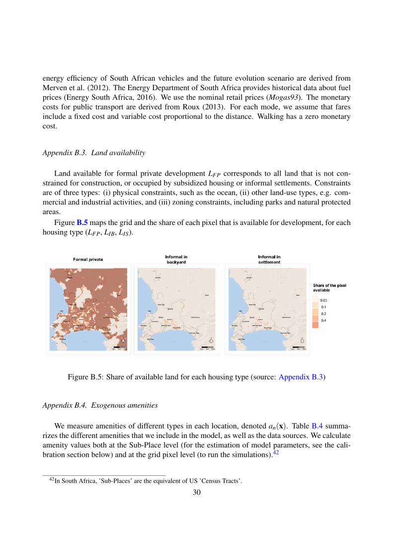
energy efficiency of South African vehicles and the future evolution scenario are derived fromMerven et al. (2012). The Energy Department of South Africa provides historical data about fuelprices (Energy South Africa, 2016). We use the nominal retail prices (Mogas93). The monetarycosts for public transport are derived from Roux (2013). For each mode, we assume that faresinclude a fixed cost and variable cost proportional to the distance. Walking has a zero monetarycost.

Appendix B.3. Land availability

Land available for formal private development LFP corresponds to all land that is not con-strained for construction, or occupied by subsidized housing or informal settlements. Constraintsare of three types: (i) physical constraints, such as the ocean, (ii) other land-use types, e.g. com-mercial and industrial activities, and (iii) zoning constraints, including parks and natural protectedareas.

Figure B.5 maps the grid and the share of each pixel that is available for development, for eachhousing type (LFP, LIB, LIS).

Figure B.5: Share of available land for each housing type (source: Appendix B.3)

Appendix B.4. Exogenous amenities

We measure amenities of different types in each location, denoted an(x). Table B.4 summa-rizes the different amenities that we include in the model, as well as the data sources. We calculateamenity values both at the Sub-Place level (for the estimation of model parameters, see the cali-bration section below) and at the grid pixel level (to run the simulations).42

42In South Africa, ’Sub-Places’ are the equivalent of US ’Census Tracts’.

30

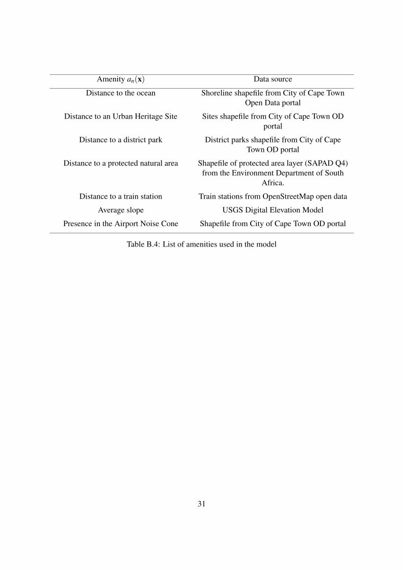
Amenity an(x) Data source

Distance to the ocean Shoreline shapefile from City of Cape TownOpen Data portal

Distance to an Urban Heritage Site Sites shapefile from City of Cape Town ODportal

Distance to a district park District parks shapefile from City of CapeTown OD portal

Distance to a protected natural area Shapefile of protected area layer (SAPAD Q4)from the Environment Department of South

Africa.

Distance to a train station Train stations from OpenStreetMap open data

Average slope USGS Digital Elevation Model

Presence in the Airport Noise Cone Shapefile from City of Cape Town OD portal

Table B.4: List of amenities used in the model

31

Appendix C. Calibration

Appendix C.1. Other data sets used for the calibration

We use the housing sales registry of the City of Cape Town. This data set includes records ofhousing transactions, including sales year, area, type, price and location of properties. We onlyconsider transactions that took place in 2011 and aggregate the sales information at the Sub-Placelevel. We calculate a median price (denoted Ps) per square meter of land for Sub-Places with morethan 20 transactions recorded. We also use a data set of average formal dwelling sizes providedby the Municipality of Cape Town, at the Transport Zone level. We aggregate the values at theSub-Place level (denoted qs).

Appendix C.2. Estimation of construction function parameters

We estimate the relation between the estimated stock of formal private housing and housingprices in cross-section to identify the parameters of the construction function {κ,a}. Combining(6) and the equilibrium condition (iv), we have:

4

∑i=1

NFPi (x)QFP(x)/LFP(x) = κ

1a .

((1−a)RFP(x)

ρ+δ

) 1−aa

(C.1)

where4

∑i=1

NFPi (x) = NFP(x) is the number of household living in formal dwellings. We regress

the log of the previous equation at the sub-place level, denoted s:

log(NFP

s)= γ1 + γ2 log(Ps)+ γ3 log(qs)+ γ4 log

(LFP

s)+ εs

where NFPs is the number of households in formal housing at the Sub-Place level, Ps is the median

price per unit of land, LFPs is the amount of available land for formal housing and qS is the dwelling

size. From equation (C.1), we expect coefficients γ3 to be close to 1 and γ4 to be close to−1. Notethat equation (C.1) theoretically only applies to formal private housing. However, because housingin low-income neighborhoods is a mix of formal private, formal subsidized housing and informalhousing, we restrict our sample for the estimation, by excluding the Sub-Places in the bottom quin-tile of property prices Ps and for which more than 5% of dwellings are reported to live in informalhousing43We also exclude rural sub-places (i.e., those that are large, with a small share than canbe urbanized). We find: log

(NFP

s)= −3.51(0.97)+ 0.25(0.07) log(Ps)− 0.98(0.07) log(qs)+

0.92(0.08) log(LFP

s), with standard errors in parenthesis. We find that coefficient γ3 is close to

1 and coefficient γ4 is close to −1. Coefficient κ and a in the construction function are retrievedfrom γ1 and γ2, with a = 1− γ2 and

κ =1

(1−a)1−a exp(γ1) .

43Our data set for dwelling sizes only provides the average dwelling size at the Sub-Place level, aggregating formaland informal housing.

32

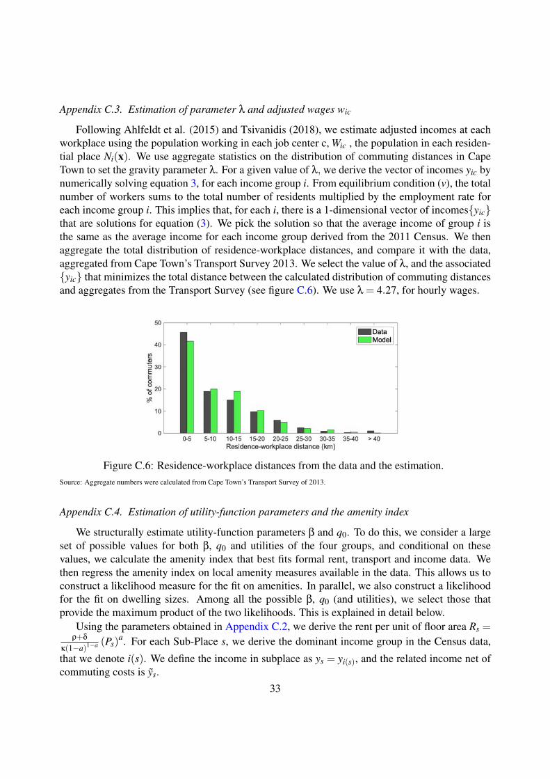
Appendix C.3. Estimation of parameter λ and adjusted wages wic

Following Ahlfeldt et al. (2015) and Tsivanidis (2018), we estimate adjusted incomes at eachworkplace using the population working in each job center c, Wic , the population in each residen-tial place Ni(x). We use aggregate statistics on the distribution of commuting distances in CapeTown to set the gravity parameter λ. For a given value of λ, we derive the vector of incomes yic bynumerically solving equation 3, for each income group i. From equilibrium condition (v), the totalnumber of workers sums to the total number of residents multiplied by the employment rate foreach income group i. This implies that, for each i, there is a 1-dimensional vector of incomes{yic}that are solutions for equation (3). We pick the solution so that the average income of group i isthe same as the average income for each income group derived from the 2011 Census. We thenaggregate the total distribution of residence-workplace distances, and compare it with the data,aggregated from Cape Town’s Transport Survey 2013. We select the value of λ, and the associated{yic} that minimizes the total distance between the calculated distribution of commuting distancesand aggregates from the Transport Survey (see figure C.6). We use λ = 4.27, for hourly wages.

Figure C.6: Residence-workplace distances from the data and the estimation.Source: Aggregate numbers were calculated from Cape Town’s Transport Survey of 2013.

Appendix C.4. Estimation of utility-function parameters and the amenity index

We structurally estimate utility-function parameters β and q0. To do this, we consider a largeset of possible values for both β, q0 and utilities of the four groups, and conditional on thesevalues, we calculate the amenity index that best fits formal rent, transport and income data. Wethen regress the amenity index on local amenity measures available in the data. This allows us toconstruct a likelihood measure for the fit on amenities. In parallel, we also construct a likelihoodfor the fit on dwelling sizes. Among all the possible β, q0 (and utilities), we select those thatprovide the maximum product of the two likelihoods. This is explained in detail below.

Using the parameters obtained in Appendix C.2, we derive the rent per unit of floor area Rs =ρ+δ

κ(1−a)1−a (Ps)a. For each Sub-Place s, we derive the dominant income group in the Census data,

that we denote i(s). We define the income in subplace as ys = yi(s), and the related income net ofcommuting costs is ys.

33

Combining equations 4 and 9 at the Sub-place level, we obtain the following relationship, forall s:

ui(s)

As= α

αβ

β ys−q0Rs

Rβs

, (C.2)

where ui(s) is the (constant) utility of income group i(s), and As is the amenity index in s.

The relationship between rents and dwelling size is given by (9):

qs = βys

Rs+(1−β)q0Rs. (C.3)

We define a range of possible values for β and q0, knowing that 0<β<1 and the minimumconsumption of housing q0 must be below the size of informal dwellings qIS = qIB = 20 m2.

For each possible value of β, q0, and ui we calculate the amenity index as:

As =ui(s)

(1−β)1−βββ ys−q0Rs

Rβs

.

In each Sub-Place, the amenity index is an aggregate of several amenities, as given by As =(∏n (an,s)

ϑi)

εA,s. We estimate the equation log(As) = ν0 +∑ϑnlog(an,s)+ log(εA,s) to identifythe set of (ϑn)q0,β conditional on q0 and β. As for the simulated dwelling sizes, they can be writtenas qs = β

ysRs+(1−β)q0Rs. We further denote εq,s the ratio of the dwelling sizes in the data (qs) and

of the simulated dwelling sizes (qs), with qs = qsεq,s. Finally, for a set of {β,q0,ui}, we estimatethe log-likelihood that the model predicts the correct income sorting. To do that, we calculate thelikelihood that the model reproduces income sorting as the likelihood of a discrete-choice logitmodel of land allocation to the highest bidder (consistently with competition for land within theformal private sector). Identifying the group with the highest bids as the dominant group in the

data, we can write the log-likelihood for income sorting as l = ∑s

(ψi(s)(s)

λinc

)−∑s log

(∑ j e

ψ j(s)λinc

),

where λinc is the scale parameter of a Gumbel maximum distribution.

We identify the coefficients {β,q0,ϑi} by maximizing the sum of log-likelihoods of the dis-tributions εA,s and εq,s (assuming that εA,s and εq,s follow a log-normal law of mean 1) plus thelog-likelihood l. We first scan a discrete set of values for the parameters. From the best solution,we then run Matlab’s ’interior-point’ algorithm to find the maximum. The obtained values forthe parameters ϑi are presented in table C.5. We use these coefficients to generate a map of theamenity index for every location of the grid (see Figure C.7).

34

Table C.5: Result of the regression on amenities

Residual utility (log)

Proximity to a district park (< 1 km) -0.015 (0.02)

Proximity to the ocean (< 2 km) 0.11∗∗∗ (0.02)

Proximity to the ocean (2< . < 4 km) 0.08∗∗∗(0.02)

Proximity to Urban Heritage Site (< 2 km) -0.01 (0.02)

Airport Noise Cone (within) -0.04 (0.03)

Slope (between 1 and 5%) 0.09∗∗∗ (0.02)

Slope (> 5%) 0.15∗∗∗ (0.02)

Proximity to a biosphere reserve (< 2 km) 0.004(0.02)

Proximity to a train station (< 2 km) -0.013 (0.02)

Constant -1.96∗∗∗ (0.02)

Observations 307R2 0.30Adjusted R2 0.28F Statistic 14.2∗∗∗ (df = 297)Note: ∗p<0.1; ∗∗p<0.05; ∗∗∗p<0.01

35

Figure C.7: Amenity score

Appendix C.5. Calibration of the informal housing parameters

We run the model for a set of values for the ’disamenity’ scores for living in an informalsettlement or in a backyard structure (BIS,BIB).44 We define a score that consists of the sumof absolute differences between the simulated and Census data shares of households living ininformal settlements and informal backyard dwellings. We select the values of BIS and BIB thatminimize this score and find BIB = 0.74 and BIS = 0.70.

Appendix C.6. Parameter values

Tables C.6 and C.7 present the chosen and calibrated parameters.36

Maximum fraction of ground surfacedevoted to housing

0.7

Transport times and costs cf. Appendix B.2

Built capital depreciation rate 2.5%

Cost associated with travel time Equal to income per minute

Dimension of an RDP/BNG house Interior space 40 m2

Backyard space 70 m2

Minimum dwelling size for formalprivate housing qmin = 31.6 m2

Table C.6: Chosen parameters

Households utility function parameter β = 0.25

Basic need in housing in the utilityfunction

q0 = 4.1

Coefficients of development function forformal private housing

a = 0.75, and κ = 0.04

Disamenity for living in a backyardshack

BBY = 0.74

Disamenity for living in a settlementshack

BIS = 0.70

Agricultural land price (in 2011) 807 R/m2

Table C.7: Estimated parameters

44Recall that the amenity for living in formal housing is normalized to 1.

37

Appendix D. Benchmark simulation

Appendix D.1. Benchmark simulation for the calibration year (2011)Figure D.8 shows the comparison between the model’s results and the data for densities and

housing prices as functions of the distance to Cape Town’s Central Station for the year 2011. Themodel captures well the main spatial trends in housing density and prices.

(a) Population density (b) Housing prices per m2 of land

Figure D.8: Comparison between simulation (green) and data (blue) for the year 2011Note: The dotted lines represent the average value of data at a given distance from Cape Town’s Central Station.

The model also allocates well households to the various housing types (see Figure D.9).

(a) Formal housing (b) Informal in backyard (c) Informal in settlement

Figure D.9: Allocation of households to housing types and spatial distributionsNote: The figure represents the distribution of households by housing type as a function of distance from Cape Town’s Central Station in 2011.Simulated values are in green, and data totals are are shown in dotted lines.

Appendix D.2. Retrospective evolution to 2001We run the model backwards to 2001 and compare the results of the simulation with local data

(at the Sub-Place level). In this retrospective simulation, we assume that transport times remainconstant, as well as the amenity index. Main inputs that vary over time include total population,

38

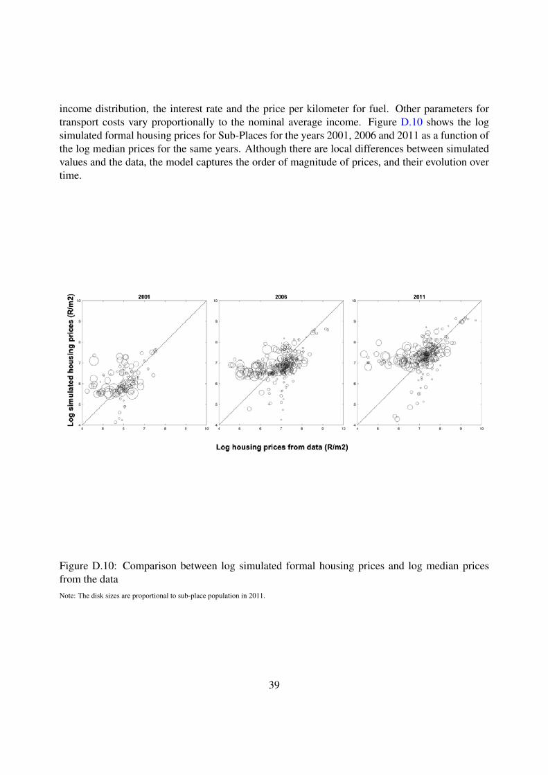
income distribution, the interest rate and the price per kilometer for fuel. Other parameters fortransport costs vary proportionally to the nominal average income. Figure D.10 shows the logsimulated formal housing prices for Sub-Places for the years 2001, 2006 and 2011 as a function ofthe log median prices for the same years. Although there are local differences between simulatedvalues and the data, the model captures the order of magnitude of prices, and their evolution overtime.

Figure D.10: Comparison between log simulated formal housing prices and log median pricesfrom the dataNote: The disk sizes are proportional to sub-place population in 2011.

39

Appendix E. Algorithm to solve for the equilibrium

Figure E.11: Solving for the equilibrium

40

Appendix F. Details of the reference scenario

We build a reference scenario at the 2040 horizon, designed to study the effect of projectedpopulation growth on the urban structure. We assume that between 2016 and 2040, populationgrows at a pace of approximately 24,000 new households per year to reach 1.77 million householdsas projected. This corresponds to a growth of 50% over 24 years.

All other input parameters are unchanged. In particular, we assume that the relative wagesbetween income groups, and for each income group the ratio between the wages for the differentemployment centers, remain constant over time. The amenity index remains constant. Transportmonetary costs (for both public transport and private cars) change over time with average income.The interest rate remains constant at 3% after 2015. We assume that transport times betweenplaces of residence (x) and employment centers (c) do not change over time. This corresponds toa situation where future investments in transport would absorb congestion induced by populationgrowth.

We extract the locations of future formal subsidized housing from a spatial data set of RDP/BNGprojects, provided by the City of Cape Town. This data set gives the location and number ofdwellings of future RDP/BNG projects, corresponding to a total of 255,000 dwellings. Moreover,it gives an indication of the project status, that we aggregate in two horizons: ’Short-term’ (as-sumed to be built before 2025) and ’Long-term’ (assumed to be built after 2025), as representedon Figure F.13. Regarding the implementation sequence for these projects, we assume that thefirst properties are uniformly distributed, first across zones for ’Short term’ projects, then acrossthe zones for ’Long term’ ones.

Figure F.12: Urban Edge (black continuous line)Note: The figure represents the Urban Edge as defined in the 2013 Municipal Spatial Development Framework (MSDF). The gray area representsthe urban footprint in 2013. Source: City of Cape Town.

41

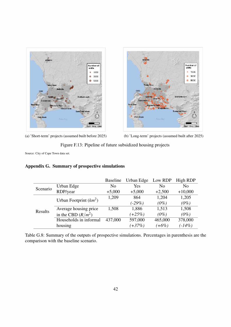
(a) ’Short-term’ projects (assumed built before 2025) (b) ’Long-term’ projects (assumed built after 2025)

Figure F.13: Pipeline of future subsidized housing projects

Source: City of Cape Town data set.

Appendix G. Summary of prospective simulations

Baseline Urban Edge Low RDP High RDP

ScenarioUrban Edge No Yes No NoRDP/year +5,000 +5,000 +2,500 +10,000

Results

Urban Footprint (km2)1,209 864 1,204 1,205

(-29%) (0%) (0%)Average housing pricein the CBD (R/m2)

1,508 1,886 1,513 1,508(+25%) (0%) (0%)

Households in informalhousing

437,000 597,000 465,000 378,000(+37%) (+6%) (-14%)

Table G.8: Summary of the outputs of prospective simulations. Percentages in parenthesis are thecomparison with the baseline scenario.

42