Working paper 5:

Assessing threats to Mongolia’s economic recovery

Abstract

This paper examines the impact of three shocks (a commodity-price drop, fiscal expansion,

and the termination of the biggest mine development) looming in Mongolia’s near future. We

modified the PEP-1-t model and calibrated it to the IMF’s recent projections in a business-as-

usual scenario. The alternative scenarios for the Mongolian economy, considering these

shocks, suggest that the impacts may be significant.

Key words: CGE model; Mongolian economy; Commodity price; Fiscal policy

JEL: D58, E62, I32, Q33

Acknowledgements

This work was carried out in the context of an Institutional Support Project with financial and

scientific support from the Partnership for Economic Policy (PEP) and funding from the

Department for International Development (DFID) of the United Kingdom (UK Aid) and the

Government of Canada through the International Development Research Center (IDRC). We

thank Helene Maisonnave, Lulit Mitik Beyene, Bernard Decaluwé and Martin Cicowiez for

their valuable comments and advice.

Authors

Ragchaasuren Galindev, Tsolmon Baatarzorig, Nyambaatar Batbayar, Oyunzul Tserendorj1

1 ragchaasuren@eri.mn, tsolmon.baatarzorig@gmail.com, nyambaa95@gmail.com, oyunzul@eri.mn

2

1. Introduction Mongolia is a resource-rich country that is heavily reliant upon mining (especially of coal and

copper). The mining sector accounts for over 80% of annual exports and 24% of budget

revenue, according to figures from the National Statistical Office (hereafter, NSO).2 The

boom-and-bust cycles of the mining sector have driven fluctuations in Mongolia’s recent

economic growth. The economy grew rapidly between 2010 and 2014, for example, with a

peak of 17% in 2011 as a consequence of high commodity prices for minerals and significant

foreign direct investment (FDI) in the Oyu Tolgoi (OT) open-pit mine, and then slowed to

1% in 2016 as a result of low commodity prices and a sharp decline in FDI.3

During the boom in 2010-2014, government expenditures increased to account for

40.1% of GDP while government revenue increased to 31.2% of GDP as of 2013. Because of

unfavorable external economic conditions that began in late 2013 (more specifically, the drop

in commodity prices), however, economic growth slowed. Government revenue consequently

fell to 23.7% of GDP in 2016 while expenditures remained high at 40.7% of GDP. This led to

a significant budget deficit of 17% of GDP. The budget deficit was moreover financed

through external debt, resulting in a public debt that stood at 87.6% of GDP in 2016. The

government of Mongolia spent over 20% of its budget revenue on interest payments alone in

2016.

Given scheduled repayments of bonds, declining international reserves, and

downgraded credit ratings, a crisis in the currency market would have been a foregone

conclusion. In response, the government initiated and reached an Extended Fund Facility

(EFF) agreement with the IMF in May 2017. Under this agreement, the government received

funding worth $5.5 billion USD (IMF’s loan of $435 million USD, a 15-billion RMB swap

line from People’s Bank of China, and budget and project support of $3 billion USD from the

ADB, WB, Japan, and Korea).4 In light of economic conditions and projections at that time,

fiscal consolidation was an essential part of the IMF program. In other words, as a part of the

program, the Mongolian government was required to cut expenditures, increase revenue,

initiate pension and public-finance-management reforms, and take measures to improve the

social safety net in order to achieve debt sustainability.

Since 2017, favorable economic conditions (continued increases in commodity prices

and FDI in OT underground-mine development, e.g.), in conjunction with the EFF program,

have blessed the economy. In addition to the recovery of the mining sector, the EFF program

has improved fiscal performance through fiscal reforms. As a result, the budget balance has

been in surplus since early 2018.

Underlying risks could make this fiscal improvement temporary, however. Given the

ongoing international trade war and global economic slowdown, for example, potential

negative shocks to commodity prices and to foreign demand are likely. Environmentally-

friendly policy reforms in China could halt demand for Mongolian coal and iron ore. In

addition, political pressure on the budget continues to be one of the most significant risks to

Mongolia’s fiscal position and, in the run up to Parliamentary elections in 2020, politicians

may unnecessarily expand public spending. Finally, a number of factors, including political

considerations, could halt OT underground mine development.

We assessed the economic impact of the three possible risks mentioned above by

modifying the PEP-1-t standard CGE model in conjunction with the Mongolian SAM 2014 as

well as with IMF projections. IMF projections provide a benchmark scenario. The results in

2 The website of the National Statistical Office is www.1212.mn. 3 Oyu Tolgoi is a large-scale copper mine in the South Gobi of Mongolia. See Fisher et al. (2011) for a study

examining its impact on the Mongolian economy. 4 This was about half of Mongolia’s annual GDP in 2017.

3

the alternative scenarios highlight the significant economic consequences of the risks.

The body of literature on CGE modelling in Mongolia is growing. Fisher et al. (2011)

used a global and recursive dynamic CGE (MINCGEM) model to analyze the economic

impact of the OT copper mine on the Mongolian economy and found a significantly positive

impact. Lkhanaajav (2016) conducted a historical simulation of the Mongolian economy by

developing two CGE models (ORANI-G and MONAGE) and found that the mining boom

resulted in a massive increase in Mongolia’s terms of trade. In addition, the manufacturing

sector lost its competitiveness while the service sector thrived. Baatarzorig et al. (2018)

examined the impact on the economy of the rapid expansion of the mining sector and a

decrease in copper price using the PEP-1-1 model calibrated to a 2010 SAM. They found

that, as a result of the structure of the Mongolian economy, rapid expansion in the mining

sector had a positive effect on the economy and produced insignificant Dutch disease effects

in other sectors.

The second shock, meanwhile, was a significant risk factor. Under PEP’s institutional

support project undertaken at the Economic Research Institute (ERI) in Mongolia, researchers

produced a series of studies. Galindev et al. (2019a) used a PEP-1-1 model linked with a

microsimulation poverty model to consider the macro and microeconomic impact of fiscal

consolidation under the IMF program, presuming various economic conditions related to

commodity and fuel prices. Galindev et al. (2019b) examined the impact of FDI in the coal

sector on the economy and environment (GHG emissions) by modifying the PEP-1-t model.

Although they considered a less sophisticated business-as-usual scenario than does this paper,

their main focus was to capture the idea of shifting from truck transportation to railway

service in exporting coal because of FDI. Galindev et al. (2019c) spelled out the construction

of a 2014 SAM used for the relevant studies. Galindev et al. (2019d) considered the same

business-as-usual scenario that we considered here and examined the impact of FDI in the

coal sector. Byambasuren et al. (2015), in an analysis based on the MINCGEM model, found

a positive impact on the domestic economy of public investment in a power plant and copper

refinery.

The questions of interest in this paper can be analyzed in macroeconomic models.

Avralt-Od et al. (2011) used a DSGE model to examine the impact of mining revenue on the

macroeconomy under alternative budget and monetary policies. Bauer et al. (2017) examined

the impact of the IMF’s EFF program and commodity-market conditions on the Mongolian

economy by developing a semi-structural macroeconomic model. Their study concluded that

the program had a small negative effect on GDP growth in the short-run while substantially

improving debt sustainability. They also found that the Mongolian economy and debt

sustainability were vulnerable to world commodity prices. The same analysis was conducted

by Galindev et al. (2019) using the same model. They found that commodity price shocks and

political risks that increased government spending could make the fiscal situation worse in

the long-run and slow economic growth.

2. Data and Methodology We modified the dynamic PEP 1-t model developed by Decaluwé et al. (2013) and calibrated

it to a 2014 Mongolian Social Accounting Matrix (SAM).

2.1. Model The PEP 1-t model is a recursive dynamic CGE model and is described fully in Decaluwé et

al. (2013). In brief, however, its main specifications are: the production side of an economy is

divided into different activities/sectors. Each sector has a nested structure, and each level uses

a production function with constant returns to scale. Specifically, the first level of production

is a Leontief function of value added and intermediate consumption. At the next level, value

4

added is a constant elasticity of substitution (CES) function of composite labor and composite

capital. Each composite input is a CES function of different types. Intermediate consumption

of each commodity, on the other hand, is proportional to production by sector. Each sector

may produce multiple commodities, which are aggregated by a constant elasticity of

transformation (CET) function. Finally, quantities to sell domestically or to export are

governed by a CET function and relative prices.

On the demand side, the consumption of a commodity is a CES function of domestic

and imported quantities. A representative household allocates its disposable income, which

derives from capital, labor, and transfers from other agents, between consumption and

savings. Its demand for commodities is governed by a linear-expenditure system. This is a

savings-driven-investment model, and the sum of household, government, and foreign

savings determines the total amount of investment. Investment demand distinguishes between

gross fixed-capital formation and changes in inventories. Government revenue from income

taxes, indirect taxes (production, commodities, and foreign trade), and transfers from other

agents are divided among savings, spending on commodities, and transfers to other agents.

Demand for commodities for investment and government spending purposes are proportional

to respective total expenditures.

Export demand for domestic commodities is an isoelastic function of relative prices

(foreign price in domestic currency divided by domestic price). Current account balance in

the balance of payments is determined by the amount of exogenous foreign savings. The

numeraire is normally the nominal exchange rate. Stock of each type of capital increased by

investment but decreased by depreciation in this model as does it in growth models (e.g.,

Solow, 1956). Investment in public services sectors is normally exogenous while that in other

sectors is endogenous depending on the return (ratio between the rental rate and user cost of

capital—the depreciation and interest rates).

We made the following modifications in the PEP-1-t model. The first modification is

introduction of the wage curve—i.e., the Phillips curve relationship between the

unemployment rate and the real wage index. Equation 1 shows this relationship in general

terms.

1

1

t t

t t t

W W U

PIXCON PIXCON U

(1)

where tW , tPIXCON and tU are nominal wage, consumer price index and the unemployment

rate in period t , and 0 was an elasticity parameter. U is a constant which is a product of

the long-term unemployment rate (NU ) and the growth rate of the real wage.5 When 1t ,

values in 1 0t indicate the base-year ones. According to Equation 1, the real wage and

unemployment rates are determined within a period. The unemployment rate converges from

0U to NU over time, and the parameter controls the speed of convergence as well as

indicates the slope of labor supply curve within t . The intuition of Equation 1 is that wage-

setters care about real wages and update the nominal wage on the basis of actual inflation but

also consider current labor market conditions through the unemployment rate.

Given (1), labor supply was written as follows:

5 In the balanced growth path simulation, one may write 1

N tU U X where the latter is the growth rate of

the real wage such that t NU U . In the simulations below, we set 7%U . Consequently, we found that the

unemployment rate converged to 6.6% over time and the real wage was updated in accordance with Equation 1.

5

1t P tLS LS U (2)

where tLS and PLS are labor supply in t and potential labor supply respectively. As we

describe below, the potential labor supply grows at the exogenous population growth rate.

The labor supply within a period, on the other hand, is not fixed as the unemployment rate

moves around its natural rate. For instance, when t NU U , we find that (1 )t P NLS LS U . In

that case, the real wage in t decreases (or grows relatively slowly) from 1t which, in turn,

reduces (or increases relatively slowly) producers’ costs. Hence, the demand for labor

increases. This process continues until t NU U . The opposite happens if t NU U .

As we discuss below, the model is calibrated to the projections of the IMF until 2022.

One of the main indicators of IMF projections is public debt. The PEP-1-t model does not

have explicit budget balance and public debt dynamics. The modified model includes the

following equation.

_t t t t tBD G GTR IT PUB YG (3)

where tBD is budget balance, tG is government spending, tGTR is total government transfers

to other institutions including interest payments, _ tIT PUB is government investment/capital

expenditure, and tYG is government revenue. Public debt, tD , accumulates in accordance

with the following equation.

1 _t t t tD D BD a D (4)

where _ ta D is an adjustment variable that accounts for the factors affecting the level of debt,

including a debt revaluation effect, write-offs, and inclusion of debts of state-owned

enterprises. We also calculated budget balance to GDP and public debt to GDP ratios. Interest

payments were exogenous for some periods taking the IMF projections and then became

endogenous as we made an assumption about the interest rate for the period beyond the IMF

projections. In essence, the following equation was added:

1t t tIP i D (5)

where tIP is interest payment and ti is the interest rate.

We separated investment among public, private, and mining sectors. In the PEP-1-t

model, public investment is calibrated from public service capital stock in the base-year,

which could be different from public investment in the budget data. Therefore, we introduced

a variable, _ tIT TR , which was calibrated to account for the difference.

, ,_ _ _t t k pub t t

k pub

IT TR IT PUB IND PK PUB (6)

where _ tIT PUB is public investment in the budget data, pub is a set of sectors providing

public services, k is type of capital, , ,k pub tIND is an additional (or new) stock in ( , )k pub , and

_ tPK PUB is an investment price index. In our model, _ tIT PUB and , ,k pub tIND were

exogenous so that _ tIT TR was endogenous.

In addition, investment in mining sectors was determined as follows:

6

,min,

min

_ _t k t t

k

IT MIN IND PK MIN (7)

where min is a set of mining sectors, _ tIT MIN is investment expenditure in mining sectors,

,min,k tIND is an additional stock in ( ,min)k , and _ tPK MIN is an investment price index.

Given _ tIT PUB and _ tIT MIN , investment in the remaining sectors, _ tIT PR is

determined as

, ,_ _ _t t t t i t i t

i

IT PR IT IT PUB IT MIN VSTK PC (8)

where tIT is total investment, ,i tVSTK is stock variation of commodity i , ,i tPC is a consumer

price of commodity i . tIT is determined as

min,

min

t t t t tIT SH SG SROW FDI (9)

where tSH is private savings, tSG is government savings (revenue over current

expenditures), tSROW is foreign savings, and min,tFDI is FDI in mining sector. The current

account balance determined tSROW because min,tFDI was exogenous from the balance of

payments equation,6

min,

min

t t tCAB SROW FDI (10)

As we followed IMF projections on interest payments, we divided government’s

transfers to the other agents into transfers related to the interest payments and other.

, , , , ,_agng GVT t agng GVT t agng t tTR TR I SHR IP (11)

where agng is a set of non-government agents, , ,agng GVT tTR is total government transfers to the

other institutions, , ,_ agng GVT tTR I is its part unrelated to the interest payments on public debt,

and ,agng tSHR is the share of interest payments transferred to agng . Because of this

modification,7 we needed to introduce an endogenous variable, , ,_ agng GVT ta TR , in the original

equation in the PEP-1-t model which became:

, , , , ,_agng GVT t t agng GVT t agng GVT tTR PIXCON TRO POP a TR (12)

where ,agng GVTTRO is initial values in the base year and tPOP is the population index. In the

simulation, we set , ,agng GVT tTR exogenously for some periods so that , ,_ agng GVT tTR I and

6 In the base-year, minFDI was set at zero so that CABO determined SROWO as in the PEP-1-t model. In the

simulations, tSROW was endogenous because tCAB followed IMF projections, and min,tFDI was exogenous.

7 Other institutions’ transfers were also modified with , ,_ ag agj ta TR .

7

, ,_ agng GVT ta TR stayed endogenous in (11) and (12) respectively. For some periods,

, ,_ agng GVT tTR I was exogenous so that both , ,agng GVT tTR and , ,_ agng GVT ta TR were endogenous.

Given min,tFDI , we needed to modify the additional capital equation as follows:

,min, ,min, min, _k t k t t tIND INDO FDI PK MIN (13)

where ,min,k tINDO is the initial value in the base-year.

Another modification was that building capital stock took more than one period. This

was reflected in the following equation.

, , 1 , , , , , , ,(1 ) _k j t k j t k j k j t k j tKD KD IND a KD (14)

where j is a set of sectors, , ,k j tKD is capital stock in ( , )k j , and , ,_ k j ta KD is a variable used

to control dynamics. For instance, it was the case that , , , ,_ k j t k j ta KD IND for three years

and, thereafter, 4

, , 4 , ,_t

k j t k j t

t

a KD IND

. The idea was to reflect the construction time of

capital during which capital stock fell because of depreciation but then increased sharply after

some period when capital became productive.

2.2. Data We built the SAM using data from 2014 including the Supply and Use Table (SUT), the

balance of payments, and government budget data from the NSO.

The detailed SAM is a square matrix with eighty-three columns and rows.8 The

accounts of the SAM consist of twenty-three sectors and twenty-five commodities; two

production factors (capital and labor); three types of institutions (private, government, and the

rest of the world); three types of taxes (income tax, import duties, and taxes on commodities);

and saving (investment) accounts divided into public investment, mining, private investment,

and changes in inventories (Table A1 in Appendix A).

Table A2 shows the macro SAM as a share of nominal GDP in 2014 (22.2 trillion

MNT). Household consumption contributed more than half of GDP (57%) while government

expenditure was 13% of GDP. Gross fixed capital formation (both public and private) and

inventory changes accounted jointly for 42% of GDP. The values of both export and import

were more than half the GDP (52% and 56%, respectively). The economy was equally

intensive in both capital and labor—i.e., the values of payments to capital owners and

compensation of employees were both 45.3% of GDP. The share of value added in GDP was

90.2%, and the remaining 9.8% came from indirect taxes on commodities (7.7%), import

duties (1.6%), and net taxes on production 0.5%).

Production structure: The livestock and trade sectors contributed most to the labor

income while mining of metal ore contributed most to the capital income. The crude oil,

metal ore, coke, and food sectors were highly intensive in capital while livestock, public

administration, education and health sectors were most intensive in labor (Table A3). The

economy as a whole was equally intensive in both labor and capital.

Trade structure: Table A4 shows the trade structure of the economy. More than half

of the total export was metal ore while the majority of imports (74%) were other

manufacturing products and fuel. Crude oil and metal ore were almost exclusively exported

8 See Galindev et al. (2019c) for the construction of the SAM.

8

while fuel and transport equipment were fully imported. Most of other manufacturing

commodities, tobacco, and accommodation were imported. On the other hand, trade and

public administration were not traded.

Demand structure: Table A5 shows the demand structure for each commodity. More

than half of final goods (food, beverage, and tobacco) and accommodation services were

consumed by households. Public administration, education, and health were mostly

consumed by the government.9 Almost all domestic coal and other mining products were

used as intermediate inputs for production. Electricity and financial activities were mainly

used as intermediate inputs as well. Trade is a 100% margin commodity while 19% of

transport services were used as margin. Construction services were mainly used for

investment purposes.

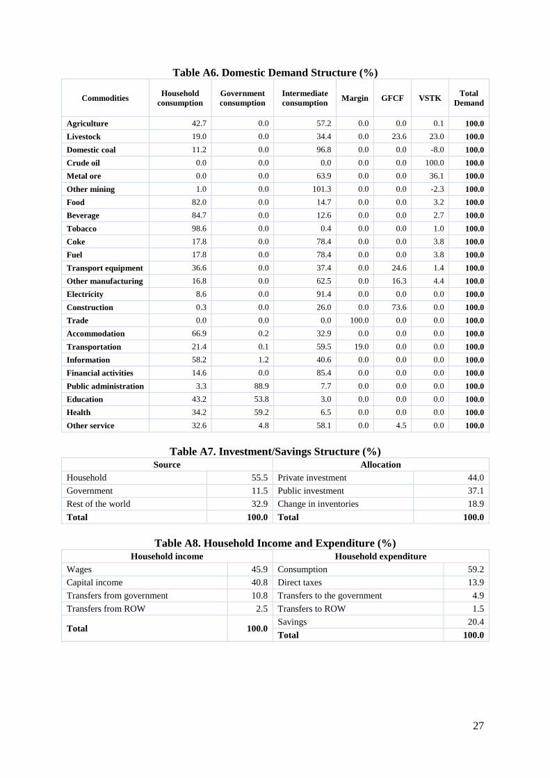
Investment/Savings structure: More than half of the total investment (adjusted by

19% for the value of stock building) was financed by household savings (Table A6).10 Rest of

the world and the government contributed 33% and 12% of total investment finance (source),

respectively. 44% and 37% of the total investment budget were dedicated to the financing of

private and public investment (gross fixed capital formation) respectively.

Structure of household (private sector) income and expenditure: The main sources

of income for households were capital ownership and labor as they jointly contributed about

87% of their total income (Table A7). Households spent most of their income (59.2%) on

commodities. 14% of income went to the government as direct taxes, and 5% of income was

transferred to the government as non-tax payments as well. Transfers to the ROW was

relatively small (1.5%) while savings were equal to about 20% of total income.

Structure of government income and expenditure: The government received the

majority of its revenue from households (firms) as direct taxes (47%) and transfers (16.7%).

Twenty-seven percent of its revenue came from commodity taxes (Table A8). Other sources

of income were relatively small. Almost a half of the budget was spent on purchasing goods

and services. 33% of its budget was received by households as transfers. Government savings

was 14% of its total budget which was used to finance its capital expenditure.

3. Scenarios and Simulation Results 3.1. BAU scenario

This scenario aimed to generate a baseline for the alternatives to be compared. In doing so,

we replicated the macroeconomic indicators projected in the IMF’s fourth review under the

EFF arrangement with the Mongolian government published in November 2018 (hereinafter,

“the IMF review”).11 The model was simulated from 2014 till 2025 by imposing actual

(2016-2017) and projected (2018-2025) macroeconomic data from the IMF review. For the

simulations, annual population growth was equal to 1.8% on average as projected by the

NSO.

Firstly, we simulated the model to target 2016 values of nominal GDP, the GDP

growth rate, government capital expenditure, government spending on goods and services,

government interest payments, government revenue, budget balance, current account balance,

and private savings in the IMF review. In addition, 2016 values of transfers between the

ROW and domestic institutions were taken from the balance of payments while household

transfers to government and direct tax revenue were calculated as residual. The value of

9 Following the United Nations national account convention, these commodities are essentially consumed by the

government. 10 Note that households and firms are aggregated in our SAM. This means that “household” savings cover all the

savings of the private sector i.e., households and firms. 11 https://www.imf.org/~/media/Files/Publications/CR/2018/cr18204.ashx

9

government transfers to the ROW was calibrated to be 35% of its interest payments while

government transfers to household was calculated as the remaining interest payments plus the

2016 value of government subsidies and transfers in the IMF review. These values are given

in Table 1 together with government revenue and debt values.12

Table 1. Data used in updating the SAM to 2016

Variables Value (million MNT) GDP share (%)

Transfers from government to ROW 330,050 1.4

Transfers from government to household 3,106,950 13.0

Transfers from household to government 727,320 3.0

Transfers from household to ROW 191,208 0.8

Transfers from ROW to government 127,922 0.5

Transfers from ROW to household 524,390 2.2

Government interest payments 943,000 3.9

Government capital expenditure 3,128,000 13.1

Government spending on goods and services 3,133,000 13.1

Government total revenue 5,624,969

23.5

Budget deficit 4,069,127

17.1

Government debt 20,967,971

87.6

Current account balance -1,507,968 -6.3

Private saving 7,252,608 30.3

GDP 23,936,040 100.0

To generate the values in Table 1, some exogenous variables turned endogenous.13

Given capital stock dynamics, we shocked the sector-specific TFP for export coal with 32%,

coke with 32%, othmin with 10%, methore with 18%, and livestock with -2% to get actual

changes in the production of corresponding sectors. The export prices of export coal and coke

were reduced by 13% to replicate the observed fall in the international coal market. For the

other commodities, we maintained initial world prices.14 The direct income tax rate was

calibrated to achieve the government revenue target. The marginal propensity to save for

households was calibrated to yield the actual private savings value. The level of uniform TFP

was calibrated such that the actual GDP value was generated.

As a result of this simulation, all endogenous variables were determined. We

compared the model-generated values of three variables with actual values from the NSO to

shed light on the model performance. For household nominal consumption, we calculated

12.5 trillion MNT (versus 13.1 trillion MNT in reality). For real export growth, the model

gave 20.1% (versus 13.9% in reality). Real import growth increased by 1.8% in the model

while it decreased by 0.2% in reality.

For the second phase of simulation period (2017-2025), we considered the projected

values of the variables in the IMF review in real terms (in 2016 prices). Some of the target

values are given in the following table.15

12 See Table 9B in Appendix B for the division of relevant exogenous and endogenous variables. 13 See Table B9 in Appendix for the division of exogenous and endogenous variables. 14 According to the World Bank, the price of copper in the world market decreased by 29% between 2014 and

2016. Copper formed the main part of the metal-ore commodity in our analysis. Using these data made the

model work differently because it yielded too much depreciation of domestic currency which, in turn, resulted in

too great an increase in the export of other commodities to be consistent with the other simulation targets. 15 See Table B9 in Appendix B for the division of relevant exogenous and endogenous variables.

10

Table 2. Key Variables in the BAU Scenario (% of GDP)

Real GDP

(trillion MNT)

Interest

payment

Capital

expenditure

Government

spending

Current

account

balance

Private saving

2017 25.2 4.0 5.5 11.4 -10.4 23.5

2018 26.7 3.6 7.9 10.8 -8.3 22.5

2019 28.4 2.8 10.0 11.2 -10.7 22.0

2020 29.8 2.3 9.4 10.9 -9.6 25.0

2021 31.3 2.0 7.9 10.9 -6.7 27.7

2022 32.8 1.9 7.4 10.9 -3.4 32.3

2023 34.8 1.6 7.4 10.9 -0.5 36.2

2024* 36.5 1.5 7.5 10.7 -0.5 36.1

2025* 38.3 1.4 7.6 10.6 -0.5 35.9

Note: * indicates that these values are not in the IMF review and were assumed by the authors.

Government capital expenditure and spending on goods and services took the exact

values in Table 2 in 2017-2023 and grew at 6% and 3.4% annually in 2024 and 2025,

respectively.

Current account balance followed IMF projections until 2023, as shown in Table 2,

and evolved at the population growth rate in 2023-2025.

Economy-wide total factor productivity (TFP) levels were calibrated for 2017-2023

such that the values of real GDP in market prices replicated IMF projections until

2023, as shown in Table 2. After 2023, uniform TFP grew at 1.9% a year, taking the

average of simulated values in 2018-2022.

The marginal propensity to save was calibrated such that the values of private savings

followed IMF projections until 2023, as shown in Table 2, and remained at 2023 level

afterwards.

The direct income tax rate was calibrated to generate the government revenue values

in the IMF review until 2023 and fixed at its 2023 value afterwards.

The interest rate on government debt was endogenous until 2023 (interest payments

followed IMF projections) but was set at 3.2%, which was an average of 2020-2023

values, from 2024 onward so that interest payments turned endogenous.

We assumed that 35% of government interest payments went to domestic institutions

while 65% was paid to the ROW as in 2016.

Government transfers, excluding interest payments to the private sector, followed

IMF projections between 2017 and 2023. Government transfers to the ROW were

represented only by interest payments for the entire simulation period. Other transfers

between institutions grew at the population growth rate. Transfers, except for interest

payments, were fixed at their 2023 values for the 2024-2025 period.

Given the assumptions and the calibrated government revenue until 2023, the budget

deficit and public debt were the same as those in the IMF review for 2017-2023.

FDI of about 11.2 trillion MNT (which financed a part of current account deficits)

flowed into the metal ore sector in 2017-2021 and built productive capital in 2021 to

reflect the OT underground copper mine.

In 2016, 2017, and 2018, the world price of coal was 13% lower, 57% higher, and

77% higher than its 2014 value, respectively, capturing actual price data from

Mongolian Customs. Between 2018 and 2025, coal price was assumed to be fixed at

2018 levels.

The world price of metal ore remained at its 2014 value for the entire simulation.

Following observed prices caused the model to behave differently in 2014-2017,

11

possibly because actual revenue from copper mines was different in the balance of

payments.

The world price of the other commodities was assumed to remain at its initial values.

In 2017-2023, sector-specific TFP in metal ore sector was 33%, 26%, 20%, 12%,

16%, 6%, and 52% higher than 2014 levels, respectively, replicating the projected

increase in production of the OT underground mine. It remained at its 2023 level in

2024-2025.

Sector-specific TFP in coal export sector was 32% higher than its 2014 level in 2016

and stayed 73% higher than 2014 from 2017 onward, replicating the observed

increase in the production of the coal-export sector.

We assumed that sector-specific TFP in the livestock sector decreased by 2% each

year to control the production of livestock sector because the low quality of grassland

had become a pressing issue that could limit future production.

We assumed that sector-specific TFP in other sectors remained constant throughout

the simulation period.

Inventory changes in livestock sector were assumed to decrease by 15% each year to

control the GDP share of the livestock sector at around 12-14%. Otherwise, it

increased to 18% because of high economic growth (reflected by the increase in

investment and the importance of livestock as an investment commodity in the SAM).

Capital income to foreigners in 2016 and 2017 took actual values in the balance of

payments. For the remaining simulation period, it was calculated using the share in

the SAM.

3.2. BAU Scenario: Simulation Results

Detailed results are given in Appendix B. According to the results, real GDP grew

significantly by an average of 5-6% every year, reaching 38 trillion MNT (expressed in 2016

prices) by 2025. Investment, which increased from 7.8 trillion MNT to 17.4 trillion MNT in

2025, was expected to be a key driver of this economic growth. On one side, this was a result

of fiscal consolidation as government savings, equal to -3.9% and 3.3% of GDP in 2016 and

2017, respectively; increased steadily to around 8.3% of GDP by 2025. At the same time,

private savings were expected to increase significantly from 23.5% of GDP in 2017 to 35.9%

of GDP in 2025. Additionally, FDI in the mining sector, especially in the OT underground

mine, and stable commodity prices contributed to economic growth by promoting investment

demand and increasing production in these sectors. In light of this stable economic growth,

the unemployment rate decreased to 6.6% while the real wage increased.

The government was expected to tighten its budget deficit from 17% of GDP in 2016

to -0.7% in 2025 through fiscal consolidation. As a result, the debt burden on the budget

steadily diminished, as reflected in the public debt to GDP ratio (expected to decrease to 44%

by 2025).

Although the simulation matched aggregate variables such as GDP, investment,

government spending, and current account balance, the composition was sometimes different

from IMF projections. In the following table, we compare the percent change in the model-

generated real exports and imports with IMF projections in 2017-2023. As can be seen, the

results are different.

Table 3. Model-Generated Real Exports and Imports vs. IMF Projections (Growth, in

Percent 2017 2018 2019 2020 2021 2022 2023

Exports in the BAU (y/y % change) 4.1 3.0 0.9 1.8 7.8 15.4 19.4

12

Exports in the IMF’s projection (y/y % change) 21.4 17.6 0.2 -0.3 7.3 7.6 13.2

Imports in the BAU (y/y % change) 8.7 6.2 14.7 1.7 1.4 6.5 16.5

Imports in the IMF’s projection (y/y % change) 25.3 25.8 7.9 0.2 3.5 1.6 5.1

3.2. Alternative Scenarios This section considers uncertainties regarding the Mongolian economy as projected in the

IMF review, including the political risk of an expansionary fiscal policy, risks regarding

investment and production of the OT underground mine, and uncertainty about the world coal

market.

Scenario 1: Expansionary Fiscal Policy Because of Political Cycles This scenario assesses the economic impact of fiscal expansion related to the upcoming 2020

parliamentary election, which coincides with the end of the EFF program.

Historical data show a pattern of significant increase in government expenditures as a

share of GDP in election years. The current government is following an agreement with the

IMF regarding spending. Public-sector workers, however, especially those in health and

education, have demanded a pay raise through actions such as strikes and demonstrations.

The government cannot increase its spending under the EFF program, though we suspect

spending will increase as soon as the EFF program is over. Given this observation, we

considered that government expenditure would increase in 2021 in Scenario 1.

The following graph shows the shocks—a 20% increase in spending on goods and

services as well as transfers to private sector and a 15% increase in capital expenditure. We

assumed that the increase in budget expenditure took place through borrowing from the

loanable fund market. In this model, budget revenue over current expenditure was called

public savings, which was a source of loanable funds alongside private and foreign savings.

We fixed foreign savings to its BAU value so that the increase in budget expenditure

increased the demand for the loanable fund.

Figure 1. Government Expenditure in 2016-2025, BAU vs Scenario 1 Current expenditure

(trillion MNT)

Capital expenditure

(trillion MNT)

Transfers to private sector

(trillion MNT)

Scenario 1: Simulation Results The impact of the expansionary fiscal policy on major macroeconomic variables in

comparison to the BAU scenario is shown in the table below. The shock was applied in 2020,

and changes occurred thereafter.

13

Table 4. Scenario 1: Macroeconomic Variables, Percent Changes with Respect to BAU

Real GDP

Real private

consumption Investment Exports Imports CPI

2020 -0.3 2.0 -8.4 -0.2 -0.3 0.4

2021 -0.6 1.8 -8.9 -0.3 -0.6 0.6

2022 -0.9 1.5 -9.1 -0.3 -0.8 0.7

2023 -1.3 1.2 -8.5 -0.3 -0.9 0.7

2024 -1.5 0.9 -8.8 -0.4 -1.1 0.8

2025 -1.7 0.7 -9.0 -0.4 -1.3 0.9

Expansionary fiscal policy promoted domestic demand through increasing demand for

public services (public administration, education, health, and water supply, e.g.) and for

investment goods. At the same time, an increase in transfers to households directly pushed up

household consumption and savings. Additional expenditures resulted in a proportional

decrease in public savings, however, ultimately resulting in a smaller total investment in the

economy than observed in the BAU scenario (about 9% lower; see Table 4). The net effect on

domestic demand was positive as reflected by the increase in the price level (CPI). Relatively

higher domestic prices may lead to lower exports by appreciating the real exchange rate (the

nominal exchange rate is the numeraire). Although higher household consumption tended to

increase imports, the negative impact of lower investment seemed to be more than offset.

Overall, real GDP decreased slightly relative to the IMF projection displayed in the BAU

scenario.

The fiscal expansions create larger budget deficits, ultimately leading to higher public

debt. As shown in Figure 2, the budget deficit increased from less than 1% of GDP to more

than 5% from 2021 onward which are larger than those in the BAU scenario. As a result, the

earlier improvements in public debt reflected in the BAU scenario disappear and the debt-to-

GDP ratio increased to around 70% in Figure 3.

Figure 2. Scenario 1: Deficit-to-GDP

Ratio (%)

Figure 3. Scenario 1: Debt-to-GDP Ratio

(%)

Production by public service providers surged as the result of increased government

spending while production in investment-driven sectors decreased relative to the BAU

scenario (Figure 4). Overall, production in all sectors, except public and food, fell as a

consequence of the lower purchasing power that was caused by the appreciation of the real

exchange rate in conjunction with a decrease in investment.

14

Figure 4. Scenario 1: Production, Percent Changes with Respect to the BAU

The expansionary fiscal policy had the same impact on employment as it did on

production. Total employment decreased slightly because of decreased production and lower

total demand (GDP). Consequently, real wages were slightly lower (Figure 5).

Figure 5. Scenario 1: Real Wage Index

Overall, loosening fiscal policy had a broad negative impact on macroeconomic

variables. Though the expansion of budget expenditure promoted household as well as

government consumption, it inhibited total savings/investments in the economy. Therefore,

expanding the budget deficit ultimately led to higher public debt and was detrimental to the

economy.

Scenario 2: Stopping OT underground Mine Development This scenario considered the impact of the OT underground mine on the Mongolian

economy. Specifically, we examined what would happen if the OT underground mine project

did not continue as planned in the BAU scenario because of political uncertainty. In order to

do this, we changed some of the assumptions in the BAU scenario that were related to FDI in

15

the metal ore sector and operation of the underground mine. Those changes were the

following:

- FDI (about 5.9 trillion MNT), which was intended to finance the construction of the

underground mine, was absent between 2019 and 2021 (Figure 6). Therefore, FDI in

the metal ore sector did not generate productive capital in 2022.

- Current account balance was adjusted to the decrease in FDI.

- The production of the OT mine remained at current levels during the whole

simulation period—i.e., production was only from the OT open-pit mine because the

underground mine would not operate for the entire simulation period. As a result, the

production of the metal ore sector did not increase as in the BAU (Figure 7). This

change was governed by sector-specific TFP in the metal ore sector.

Figure 6. Scenario 2: FDI in the Metal

Ore Sector (Trillion MNT)

Figure 7. Scenario 2: Production in the

Metal Ore Sector

Scenario 2: Simulation Results There was no change in 2016-2018 because the shocks were applied beginning in 2019

(Table 5). As can be seen, all macroeconomic variables except real public consumption

decreased. Real public consumption increased as a consequence of lower prices which were

reflected by the consumer price index (CPI). Changes in macroeconomic variables were

smaller in 2019-2022 except for the sharp decline in investment in 2019 that was related to

the absence of FDI in the metal ore sector. On the other hand, the impact of negative shocks

was much bigger in 2023-2025 than in previous years because of both the decrease in FDI

and the decrease in metal ore-sector production as shown in Figures 6 and 7. For instance,

exports decreased by over 28.1% in 2025, caused mainly by the fall in metal ore production

despite the depreciation of the real exchange rate. Real GDP decreased by around 7% in

2023-2025. Overall, cancelling the OT underground mine project has a major negative impact

on the economy.

Table 5. Scenario 2: Macroeconomic Variables, Percent Changes with Respect to BAU

Real

GDP

Real private

consumption

Real public

consumption Investment Exports Imports CPI

2016 0.0 0.0 0.0 0.0 0.0 0.0 0.0

2017 0.0 0.0 0.0 0.0 0.0 0.0 0.0

2018 0.0 0.0 0.0 0.0 0.0 0.0 0.0

2019 -2.4 -1.6 8.1 -35.4 3.1 -14.0 -5.3

16

2020 -1.2 -0.7 5.5 -20.8 2.1 -8.6 -3.5

2021 -1.3 -0.9 5.4 -19.0 -0.2 -8.6 -3.6

2022 -3.0 -2.3 9.3 -12.4 -12.7 -10.7 -6.2

2023 -7.0 -5.3 20.9 -25.3 -27.3 -22.8 -13.1

2024 -7.3 -5.6 22.8 -26.8 -28.5 -24.0 -13.9

2025 -7.6 -5.8 22.5 -26.9 -28.1 -23.9 -13.7

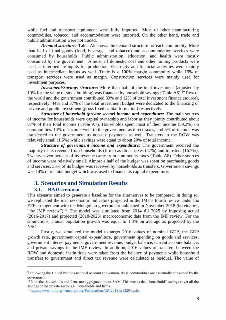
Figures 8 and 9 compare GDP in market prices and growth rates. GDP decreased

significantly while the growth rate lay on a totally different path from that in the BAU

scenario. For instance, the growth rate was 1.7% in Scenario 2 as opposed to 5.9% in the

BAU scenario in 2023.

Figure 8. Scenario 2: GDP (Trillion

MNT)

Figure 9. Scenario 2: Growth rates (%)

The deficit-to-GDP and debt-to-GDP ratios were higher in Scenario 2 than in the

BAU scenario, and the differences became bigger over time. In addition, budget deficit and

government debt started to increase beginning in 2023 (Figures 10 and 11). Thus, the budget

deficit and public debt would be much higher in the long-term if the OT underground mine

were not operational.

17

Figure 10. Scenario 2: Deficit-to-GDP

Ratio (%)

Figure 11. Scenario 2: Debt-to-GDP Ratio

(%)

As shown in Figure 12, the real wage index decreased in 2019 and then increased

slightly. However, it remained much lower than that in the BAU scenario for the entire

simulation period because of less demand for labor.

Figure 12. Scenario 2: Real Wage Index

Government revenue decreased with respect to the BAU in 2019-2022 and 2023-2025

because of decreased tax income (Figure 13).

18

Figure 13. Scenario 2: Government Revenue (Trillion MNT in 2016 prices)

Figure 14 shows that the changes in production of sectors were different depending on

the direct and indirect effects of cancelled FDI and the operation of the OT underground mine

in Scenario 2. More profound changes occurred between 2023 and 2025. All mining sectors

except metal ore experienced a small positive change (around 0-3%) while agriculture, food,

public sectors (health, education and public administration), accommodation, and other

manufacturing expanded at different rates (2-47%), a finding that can be explained by the

depreciation of the real exchange rate. In contrast, some sectors experienced contractions. For

instance, the construction sector experienced a large drop in production because its services

were mainly used for investment purposes (around 74%). Also clear is that production

increased in 2019 and 2020 and then, because of the huge reduction in the production of the

metal ore sector, declined sharply in sectors such as transportation, electricity, and financial

activities, which mainly produced intermediate inputs for other sectors.

Figure 14. Scenario 2: Production, Percent Changes with Respect to BAU

Scenario 3: Negative Shock to the Coal Sector In this scenario, we considered a negative shock in coal export and coke (which includes

19

washed coal) sectors. Specifically, world export prices of coal and coke decreased by 10% in

2019 and 2020 and thereafter stayed at 2020 levels. In addition, sector-specific TFP in coal

export and coke sectors was 20% lower than BAU levels starting in 2019, reflecting their

reduction in production. We also considered that the domestic coal sector would shrink as

domestic coal was used mainly by coke sector as an intermediate input. Therefore, TFP in the

domestic coal sector decreased as well.

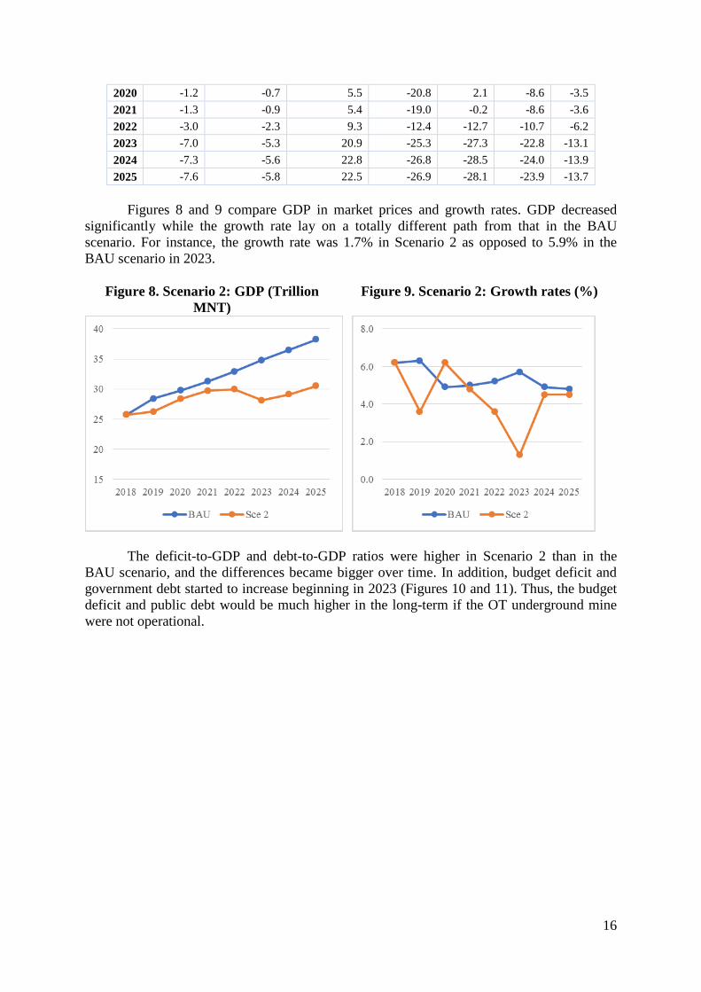
Scenario 3: Simulation Results Table 6 shows changes in macroeconomic variables. As can be seen, there are no changes in

2016-2018 because the shocks began in 2019. Real public consumption increased because of

lower prices as reflected by the consumer price index (CPI) leading to the depreciation of the

real exchange rate while other macroeconomic variables decrease in 2019-2023. Investment

decreased most because of decreased private investment, which was mainly affected by price

and demand for investment commodities. The effect of decreased exports of coal and coke

dominated the increased export of other commodities and, hence, total exports decreased.

Real GDP is lower than its BAU level by around 6% each year. Overall, the decrease in

world price of coal and coke combined with decreases in these sectors’ production had a

negative impact on the macroeconomic variables.

Table 6. Scenario 3: Macroeconomic variables, Percent Changes with Respect to BAU

Real

GDP

Real private

consumption

Real public

consumption Investment Exports Imports CPI

2016 0.0 0.0 0.0 0.0 0.0 0.0 0.0

2017 0.0 0.0 0.0 0.0 0.0 0.0 0.0

2018 0.0 0.0 0.0 0.0 0.0 0.0 0.0

2019 -4.5 -3.7 5.2 -9.8 -2.7 -6.3 -3.7

2020 -6.1 -5.0 7.3 -13.3 -2.3 -8.2 -5.1

2021 -6.4 -5.2 7.6 -14.5 -2.2 -8.6 -5.2

2022 -6.2 -5.0 7.1 -14.6 -1.6 -8.1 -4.7

2023 -5.7 -4.7 5.9 -12.4 -1.1 -6.7 -3.8

2024 -5.9 -4.9 5.8 -12.5 -1.3 -6.9 -3.7

2025 -6.1 -5.1 5.8 -12.9 -1.5 -7.2 -3.7

Nominal GDP remained significantly lower than in the BAU scenario. Real GDP

growth dropped sharply in 2019 and then rose rapidly to a peak of 6.5% in 2023. After that,

growth slowed to 5% (Figure 17).

20

Figure 15. Scenario 3: GDP (Trillion MNT) Figure 16. Scenario 3: Growth rate (%)

As shown in Figures 18 and 19, trends in the deficit-to-GDP ratio and debt-to-GDP

ratio decreased in both scenarios after 2019. However, both ratios were higher in Scenario 3.

Figure 17. Scenario 3: Deficit-to-GDP

Ratio (%)

Figure 18. Scenario 3: Debt-to-GDP Ratio

(%)

The real wage index increased in Scenario 3, but it was slightly lower than BAU

projections for each year (Figure 20).

Figure 19. Scenario 3: Real Wage Index

21

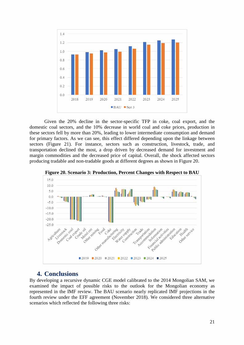
Given the 20% decline in the sector-specific TFP in coke, coal export, and the

domestic coal sectors, and the 10% decrease in world coal and coke prices, production in

these sectors fell by more than 20%, leading to lower intermediate consumption and demand

for primary factors. As we can see, this effect differed depending upon the linkage between

sectors (Figure 21). For instance, sectors such as construction, livestock, trade, and

transportation declined the most, a drop driven by decreased demand for investment and

margin commodities and the decreased price of capital. Overall, the shock affected sectors

producing tradable and non-tradable goods at different degrees as shown in Figure 20.

Figure 20. Scenario 3: Production, Percent Changes with Respect to BAU

4. Conclusions By developing a recursive dynamic CGE model calibrated to the 2014 Mongolian SAM, we

examined the impact of possible risks to the outlook for the Mongolian economy as

represented in the IMF review. The BAU scenario nearly replicated IMF projections in the

fourth review under the EFF agreement (November 2018). We considered three alternative

scenarios which reflected the following three risks:

22

In coming years, political risk may put pressure on the budget because of the 2020

parliamentary election, which will coincide with the end of the EFF program. Thus,

we considered a scenario in which budget expenditures were increased for reasons

related to politics and found that increased expenditures had negative effects on the

condition of the economy and budget. Given the results from this scenario, authorities

should be aware that any political pressure on the budget will have a severe negative

impact on the economy, and the debt burden will become a more salient issue.

We analyzed the impact of the development of the OT underground mine, one of the

most significant mining projects in Mongolia. To do so, we considered a scenario in

which the assumptions of the BAU scenario, related to the development of the

underground mine (i.e., FDI and expansion of production in the metal ore sector),

were removed. We found that the absence of the development of the underground

mine would have negative impact on the economy and would increase debt burden.

The last scenario considered a negative shock (price drop and reduction in production)

in the coal export sector. Reflecting the fact that the coal export sector is hugely

significant for the economy, the shock was found to have a severe impact on both the

economy and budget.

Overall, the above risks could be considered significant given the results of the

simulations and deserve the full attention of policy makers and general public. If these

negative shocks were to occur simultaneously, moreover, the economy will be hit very hard.

23

References

Avralt-Od, P., Bumchimeg, G., and Davaadalai, B. (2011). Macroeconomic Policy of Natural

Resources Countries. Journal of Central Bank of Mongolia, 6, 453-477.

Bauer, A., Galindev, R., Lkhagvajav, M.-O., Mihalyi, D., and Tuvaan, N. (2017). Fiscal

Sustainability in Mongolia. Ulaanbaatar, Mongolia: Natural Resource Governance

Institute.

Fisher, B., Batdelger, T., Gurney, A., Galindev, R., Begg, M., Buyantsogt, B., Lkhanaajav,

E., and Chadraaval, B. (2011). The Development of the Oyu Tolgoi Copper Mine: An

Assessment of the Macroeconomic Consequences for Mongolia. School of Economic

Studies, National University of Mongolia and BAEconomics Pty Ltd.

Baatarzorig, T., Batbayar, N., and Galindev, R. (2019). Fiscal Sustainability in Mongolia

2018. Ulaanbaatar, Mongolia: Natural Resource Governance Institute.

Baatarzorig, T., Galindev, R., and Maisonnave, H. (2018). Effects of Ups and Downs of the

Mongolian Mining Sector. Environment and Development Economics, 23(5), 527-

542.

Byambasuren, T., Purevjav, A., and Erdenekhuyag, E. (2015). Economic Impacts of the

Government Investment Policy: Dynamic CGE Model. International Journal of System

Dynamics Applications, 4(1), 96-118.

Decaluwé, B., Lemelin, A., Robichaud, V., and Maissonnave, H. (2013). The PEP Standard

Single-Country, Recursive Dynamic CGE Model. Partnership for Economic Policy.

Available at https://www.pep-net.org/pep-standard-cge-models.

Galindev, R., Baatarzorig, T., Batbayar, N., Begz, D., Davaa, U., and Tserendorj, O. (2019a).

Impact of Fiscal Consolidation on the Mongolian Economy. Partnership for Economic

Policy Working Paper Series, Working Paper 1. Available at

https://papers.ssrn.com/sol3/papers.cfm?abstract_id=3455319 Galindev, R., Baatarzorig, T., Batbayar, N., Begz, D., Davaa, U., and Tserendorj, O. (2019b).

Economic and Environmental Impact of Foreign Direct Investment in the Mongolian

Coal Export Sector. Partnership for Economic Policy Working Paper Series, Working

Paper 2. Available at https://papers.ssrn.com/sol3/papers.cfm?abstract_id=3455321

Galindev, R., Baatarzorig, T., Batbayar, N., Begz, D., Davaa, U., and Tserendorj, O. (2019c).

Mongolian Social Accounting Matrix 2014. Partnership for Economic Policy Working

Paper Series, Working Paper 3.

Galindev, R., Baatarzorig, T., Batbayar, N., Beyene, L.M., Davaa, U., and Tserendorj, O.

(2019d). Impact of FDI in the Coal Export Sector on the Mongolian Economy.

Partnership for Economic Policy Working Paper Series, Working Paper 4.

International Monetary Fund (November, 2018). Mongolia: Fifth Review Under the Extended

Fund Facility Arrangement and Request for Modification and Waiver of Applicability of

Performance Criteria-Press Release; Staff Report; Staff Supplement; and Statement by

the Executive Director for Mongolia. Available at

https://www.imf.org/en/Publications/CR/Issues/2018/11/02/Mongolia-Fifth-Review-

Under-the-Extended-Fund-Facility-Arrangement-and-Request-for-46323 Lkhanaajav, E. (2016). Mongolia's Resource Boom: A CGE Analysis. (Unpublished doctoral

dissertation.) Victoria University, Centre of Policy Studies, Melbourne, Australia.

National Statistical Office (2016, February 25). Household Socio-Economic Survey-2014.

Retrieved from http://web.nso.mn/nada/index.php/catalog/106.

24

Appendix А—SAM Table A1. Accounts in the SAM

Sectors (22) Commodities (25) Institutions (3)

1. Agriculture Agriculture Private/Households (H)

2. Livestock Livestock Government (GVT)

3. Domestic coal Domestic coal Rest of the world (ROW)

4. Coal export Coal export

5. Crude Oil Crude Oil Taxes (3)

6. Metal Ore Metal Ore Income taxes (TD)

7. Other mining Other mining Import duties (TM)

8. Food Food Taxes on commodities (TI)

9. Coke Beverage

10. Other manufacturing Tobacco Factors (2)

11 Electricity Coke Labor (Lab)

12. Water supply Fuel Capital (Cap)

13. Construction Transport equipment

14 Trade Other manufacturing Savings-Investment (4)

15. Accommodation Electricity Public investment (IT_PUB)

Changes in inventories (VSTK)

16. Transportation Construction Mining investment (IT_MIN)

17. Information Trade Private investment (IT_PR)

18. Financial activities Accommodation Changes in inventories (VSTK)

19. Public administration Transportation

20. Education Information Capital accounts (3)

21. Health Financial activities Households (Cap-H)

22. Other service Public administration Government (Cap-GOV)

23. Education Rest of the world (Cap-ROW)

24. Health

25. Other service

Notes: The names of sectors and commodities represent broader activities and a larger set of commodities. Here

we clarify a few of these; the rest are self-explanatory. Water supply represents water supply, sewerage, waste

management, and remediation activities. Information represents information and communication. Professional

represents professional, scientific, and technical activities. Financial activities represent real estate, insurance,

and other financial services.

25

Table A2. Macro SAM 2014 (% of GDP) 1 2 3 4 5 6 7 8 9 10 11 12 13 14

1 Labor

0.4 44.8

45.3

2 Capital

0.03 45.3

45.3

3 Households 43.9 39.1

10.4 2.4

95.7

4 Government 4.7 13.3 1.6 7.7 0.3 0.5 0.0 28.2

5 TD 13.3 13.3

6 TM 1.6 1.6

7 TI 7.7 7.7

8 ROW 1.4 6.3 1.5 0.8 56.4 66.4

9 Sectors 137.7 48.1 185.8

10 Commodities 56.6 13.0 95.1 16.7 3.5 28.6 6.6 220.1

11 Export 51.6 51.6

12 Investment 19.6 4.1 11.6 35.2

13 VSTK

6.6

6.6

14 TOTAL 45.3 45.3 95.7 28.2 13.3 1.6 7.7 66.4 185.8 220.1 51.6 35.2 6.6

Note: TD denotes direct taxes, TM is import duties, TI is other indirect taxes, ROW stands for the rest of the

world, and VSTK denotes stock variations.

Table A3. Production Structure (%)

Sector Labor Capital Value Added

Value

added/

Total

output

Factor intensity

Labor Capital

Agriculture 1.3 1.7 1.5 41.6 43.1 56.9

Livestock 23.7 3.2 13.4 77.6 87.9 12.1

Domestic coal 0.3 0.5 0.4 27.9 37.5 62.5

Coal export 0.8 1.4 1.1 27.9 37.5 62.5

Crude oil 0.1 4.3 2.2 39.3 2.6 97.4

Metal ore 6.6 19.6 13.1 40.7 25.2 74.8

Other mining 0.9 1.1 1.0 33.1 46.1 53.9

Food 1.2 7.1 4.2 31.0 14.6 85.4

Coke 0.2 3.2 1.7 50.8 5.0 95.0

Other manufacturing 3.5 4.2 3.8 39.0 45.3 54.7

Electricity 1.8 1.3 1.6 37.1 59.0 41.0

Water supply 0.5 0.3 0.4 35.0 61.8 38.2

Construction 4.2 5.7 4.9 22.0 42.1 57.9

Trade 17.5 8.0 12.7 64.7 68.5 31.5

Transportation 6.2 4.7 5.5 40.0 56.4 43.6

Accommodation 1.2 0.7 1.0 38.6 63.7 36.3

Information 1.7 3.3 2.5 54.0 34.3 65.7

Financial activities 3.0 7.3 5.2 78.3 29.0 71.0

Public administration 7.3 1.8 4.5 59.9 80.4 19.6

Education 8.0 1.9 5.0 76.5 80.6 19.4

Health 3.5 0.6 2.1 60.6 85.0 15.0

Other services 6.2 18.4 12.3 61.1 25.2 74.8

Total 100% 100% 100% 48.5

49.7 50.3

Table A4. Trade Structure (%)

26

Commodities Export share Import share Export intensity Import

penetration

Agriculture 0.3 0.7 4.5 11.5

Livestock 3.6 0.2 11.4 0.8

Domestic coal 0.0 0.0 0.0 0.2

Coal export 7.4 0.0 100.0 0.0

Crude oil 10.5 0.0 99.4 0.0

Metal ore 53.2 0.0 99.4 0.5

Other mining 1.0 0.2 54.9 17.4

Food 0.1 5.2 0.8 25.2

Beverage 0.0 0.8 0.1 13.1

Tobacco 0.0 0.8 5.3 60.7

Coke 4.6 0.0 72.5 0.0

Fuel 0.0 17.8 0.0 100.0

Transport equipment 0.0 7.5 75.2 100.0

Other manufacturing 8.8 41.7 35.9 75.8

Electricity 0.0 1.9 0.1 20.0

Construction 0.3 1.3 0.8 3.6

Accommodation 2.9 5.2 62.4 77.7

Transportation 3.4 2.1 13.1 10.0

Information 0.2 1.3 2.9 17.5

Financial activities 0.3 2.1 2.1 16.8

Education 0.1 1.4 0.9 11.7

Health 0.0 0.8 0.5 13.5

Other service 3.1 9.0 6.8 19.6

Total 100% 100%

Table A5. The Government Budget (%)

Government revenue Government expenditure

Transfers from households 16.7 Transfers to households 36.7

Direct taxes /TD/ 47.3 Transfers to ROW 2.8

Import duties /TM/ 5.7 Public consumption 46.1

Export taxes 0.003 Savings 14.4

Net taxes on products /TI/ 27.4

Total 100.0 Transfers from ROW 1.1

Net taxes on production 1.8

Total 100.0

27

Table A6. Domestic Demand Structure (%)

Commodities Household

consumption

Government

consumption

Intermediate

consumption Margin GFCF VSTK

Total

Demand

Agriculture 42.7 0.0 57.2 0.0 0.0 0.1 100.0

Livestock 19.0 0.0 34.4 0.0 23.6 23.0 100.0

Domestic coal 11.2 0.0 96.8 0.0 0.0 -8.0 100.0

Crude oil 0.0 0.0 0.0 0.0 0.0 100.0 100.0

Metal ore 0.0 0.0 63.9 0.0 0.0 36.1 100.0

Other mining 1.0 0.0 101.3 0.0 0.0 -2.3 100.0

Food 82.0 0.0 14.7 0.0 0.0 3.2 100.0

Beverage 84.7 0.0 12.6 0.0 0.0 2.7 100.0

Tobacco 98.6 0.0 0.4 0.0 0.0 1.0 100.0

Coke 17.8 0.0 78.4 0.0 0.0 3.8 100.0

Fuel 17.8 0.0 78.4 0.0 0.0 3.8 100.0

Transport equipment 36.6 0.0 37.4 0.0 24.6 1.4 100.0

Other manufacturing 16.8 0.0 62.5 0.0 16.3 4.4 100.0

Electricity 8.6 0.0 91.4 0.0 0.0 0.0 100.0

Construction 0.3 0.0 26.0 0.0 73.6 0.0 100.0

Trade 0.0 0.0 0.0 100.0 0.0 0.0 100.0

Accommodation 66.9 0.2 32.9 0.0 0.0 0.0 100.0

Transportation 21.4 0.1 59.5 19.0 0.0 0.0 100.0

Information 58.2 1.2 40.6 0.0 0.0 0.0 100.0

Financial activities 14.6 0.0 85.4 0.0 0.0 0.0 100.0

Public administration 3.3 88.9 7.7 0.0 0.0 0.0 100.0

Education 43.2 53.8 3.0 0.0 0.0 0.0 100.0

Health 34.2 59.2 6.5 0.0 0.0 0.0 100.0

Other service 32.6 4.8 58.1 0.0 4.5 0.0 100.0

Table A7. Investment/Savings Structure (%)

Source Allocation

Household 55.5 Private investment 44.0

Government 11.5 Public investment 37.1

Rest of the world 32.9 Change in inventories 18.9

Total 100.0 Total 100.0

Table A8. Household Income and Expenditure (%)

Household income Household expenditure

Wages 45.9 Consumption 59.2

Capital income 40.8 Direct taxes 13.9

Transfers from government 10.8 Transfers to the government 4.9

Transfers from ROW 2.5 Transfers to ROW 1.5

Total 100.0 Savings 20.4

Total 100.0

28

APPENDIX B—BAU scenario

Figure B1. BAU Scenario: Real GDP in Trillion MNT and Annual Growth (%)

29

Figure B2. BAU Scenario: Budget

Indicators as GDP Share (%)

Figure B3. BAU Scenario: Public Debt as

GDP Share (%)

30

Figure B4. BAU Scenario: Total

Investment/Savings (Trillion MNT)

Figure B5. BAU Scenario: Public and

Private Savings of GDP Share (%)

Figure B6. BAU Scenario: Real Wage

Index

Figure B7. BAU Scenario:

Unemployment Rate (%)

31

Table B8. BAU Scenario: GDP Share of Sectors

Sectors 2016 2017 2018 2019 2020 2021 2022 2023 2024 2025

Agriculture 1.3 1.1 1.1 1.1 1.1 1.1 1.0 0.9 0.9 0.9

Livestock 10.3 9.7 9.1 9.1 10.2 10.5 11.6 12.3 12.4 12.4

Domestic coal 1.4 2.8 3.5 3.3 3.3 3.4 3.1 2.4 2.4 2.5

Export coal 1.1 5.9 7.4 6.9 7.1 7.3 6.6 5.4 5.4 5.6

Crude oil 2.4 1.9 2.0 1.8 1.8 1.8 1.6 1.3 1.3 1.3

Metal ore 16.5 14.1 13.1 11.3 11.0 11.7 12.2 11.0 11.2 11.8

Other mining 1.1 1.1 1.2 1.2 1.2 1.2 1.2 1.2 1.2 1.1

Food 4.1 3.0 3.2 3.6 3.3 3.0 2.2 1.4 1.4 1.4

Coke 0.7 2.2 2.4 2.3 2.4 2.4 2.3 2.1 2.1 2.1

Manufacture 4.3 3.7 3.7 3.5 3.5 3.5 2.8 2.0 2.0 2.0

Electricity 1.6 1.3 1.2 1.2 1.1 1.1 1.3 1.4 1.4 1.4

Water 0.5 0.6 0.6 0.6 0.6 0.6 0.5 0.5 0.5 0.5

Construction 4.0 4.5 4.7 5.3 5.8 5.6 6.6 8.6 8.6 8.3

Trade 12.1 12.3 12.1 12.7 12.5 12.1 12.5 13.8 13.8 13.5

Accommodation 5.7 5.7 5.5 5.6 5.5 5.4 5.7 6.4 6.4 6.2

Transportation 1.0 0.9 0.9 0.8 0.8 0.8 0.7 0.6 0.6 0.6

Information 2.5 2.3 2.2 2.4 2.3 2.2 2.1 2.1 2.0 2.0

Finance 5.5 5.1 5.0 5.0 4.9 4.9 5.2 5.7 5.6 5.5

Public admin 4.4 3.8 3.6 3.8 3.7 3.7 3.8 4.0 4.0 3.9

Education 4.8 4.0 4.0 4.3 4.2 4.1 3.9 3.8 3.8 3.7

Health 2.0 1.7 1.6 1.8 1.7 1.7 1.7 1.7 1.7 1.7

Other activities 13.1 12.4 12.1 12.5 12.0 11.9 11.5 11.6 11.7 11.7

Table B9. Exogenous and Endogenous Variables in the BAU Scenario Year Exogenous Endogenous Notes

2014-2025 _ tIT PUB _ tIT Trans

2017-2022 tIP ti Switch places for 2023-25

2017-2022 tTDH 1ttdh Switch places for 2023-25

2014-2016 , ,ag agj tTR , , , ,_ , _ag agj t ag agj ta TR TR i

2017-2025 , ,_ ag agj tTR i , , , ,_ ,ag agj t ag agj ta TR TR

2017-2022 _ _ tGDP MP REAL tTFP Switch places for 2023-25

2014-2022 tSH 1tsh Switch places for 2023-25

2014-2025 min,,t tCAB FDI tSROW

2014-2022 tD _ ta D Switch places for 2023-25

Notes: As in the PEP-1-t model, we considered the usual exogenous variables—i.e., rates and intercepts;

export and import prices of each commodity; household minimum consumption of each commodity;

potential labor supply; stock variation of each commodity; new capital created in public and mining sectors;

the nominal exchange rate as the numeraire, nominal government spending on goods and services; current

account balance; FDI; and , ,_ k j ta KD sector-specific total factor productivity.