Assessing the relative efficiency of fluvial and glacial...
17
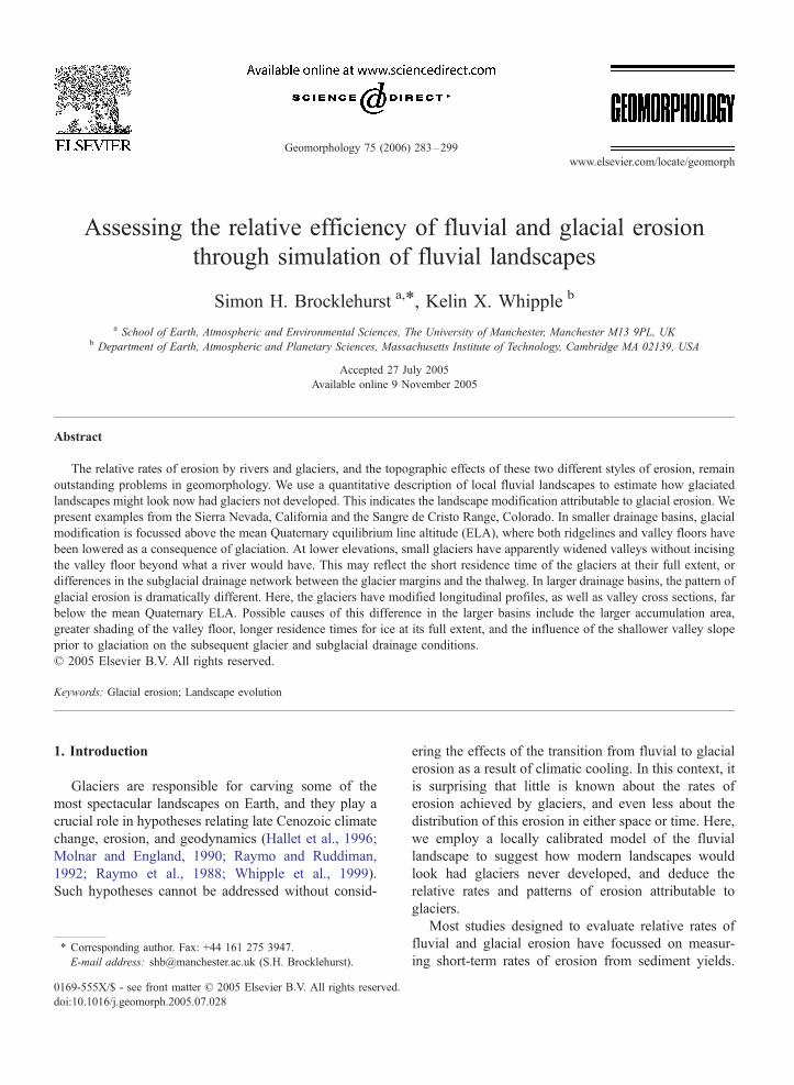
Assessing the relative efficiency of fluvial and glacial erosion through simulation of fluvial landscapes Simon H. Brocklehurst a, * , Kelin X. Whipple b a School of Earth, Atmospheric and Environmental Sciences, The University of Manchester, Manchester M13 9PL, UK b Department of Earth, Atmospheric and Planetary Sciences, Massachusetts Institute of Technology, Cambridge MA 02139, USA Accepted 27 July 2005 Available online 9 November 2005 Abstract The relative rates of erosion by rivers and glaciers, and the topographic effects of these two different styles of erosion, remain outstanding problems in geomorphology. We use a quantitative description of local fluvial landscapes to estimate how glaciated landscapes might look now had glaciers not developed. This indicates the landscape modification attributable to glacial erosion. We present examples from the Sierra Nevada, California and the Sangre de Cristo Range, Colorado. In smaller drainage basins, glacial modification is focussed above the mean Quaternary equilibrium line altitude (ELA), where both ridgelines and valley floors have been lowered as a consequence of glaciation. At lower elevations, small glaciers have apparently widened valleys without incising the valley floor beyond what a river would have. This may reflect the short residence time of the glaciers at their full extent, or differences in the subglacial drainage network between the glacier margins and the thalweg. In larger drainage basins, the pattern of glacial erosion is dramatically different. Here, the glaciers have modified longitudinal profiles, as well as valley cross sections, far below the mean Quaternary ELA. Possible causes of this difference in the larger basins include the larger accumulation area, greater shading of the valley floor, longer residence times for ice at its full extent, and the influence of the shallower valley slope prior to glaciation on the subsequent glacier and subglacial drainage conditions. D 2005 Elsevier B.V. All rights reserved. Keywords: Glacial erosion; Landscape evolution 1. Introduction Glaciers are responsible for carving some of the most spectacular landscapes on Earth, and they play a crucial role in hypotheses relating late Cenozoic climate change, erosion, and geodynamics (Hallet et al., 1996; Molnar and England, 1990; Raymo and Ruddiman, 1992; Raymo et al., 1988; Whipple et al., 1999). Such hypotheses cannot be addressed without consid- ering the effects of the transition from fluvial to glacial erosion as a result of climatic cooling. In this context, it is surprising that little is known about the rates of erosion achieved by glaciers, and even less about the distribution of this erosion in either space or time. Here, we employ a locally calibrated model of the fluvial landscape to suggest how modern landscapes would look had glaciers never developed, and deduce the relative rates and patterns of erosion attributable to glaciers. Most studies designed to evaluate relative rates of fluvial and glacial erosion have focussed on measur- ing short-term rates of erosion from sediment yields. 0169-555X/$ - see front matter D 2005 Elsevier B.V. All rights reserved. doi:10.1016/j.geomorph.2005.07.028 * Corresponding author. Fax: +44 161 275 3947. E-mail address: [email protected] (S.H. Brocklehurst). Geomorphology 75 (2006) 283 – 299 www.elsevier.com/locate/geomorph
Transcript of Assessing the relative efficiency of fluvial and glacial...
www.elsevier.com/locate/geomorph
Geomorphology 75 (
Assessing the relative efficiency of fluvial and glacial erosion
through simulation of fluvial landscapes
Simon H. Brocklehurst a,*, Kelin X. Whipple b
a School of Earth, Atmospheric and Environmental Sciences, The University of Manchester, Manchester M13 9PL, UKb Department of Earth, Atmospheric and Planetary Sciences, Massachusetts Institute of Technology, Cambridge MA 02139, USA
Accepted 27 July 2005
Available online 9 November 2005
Abstract
The relative rates of erosion by rivers and glaciers, and the topographic effects of these two different styles of erosion, remain
outstanding problems in geomorphology. We use a quantitative description of local fluvial landscapes to estimate how glaciated
landscapes might look now had glaciers not developed. This indicates the landscape modification attributable to glacial erosion. We
present examples from the Sierra Nevada, California and the Sangre de Cristo Range, Colorado. In smaller drainage basins, glacial
modification is focussed above the mean Quaternary equilibrium line altitude (ELA), where both ridgelines and valley floors have
been lowered as a consequence of glaciation. At lower elevations, small glaciers have apparently widened valleys without incising
the valley floor beyond what a river would have. This may reflect the short residence time of the glaciers at their full extent, or
differences in the subglacial drainage network between the glacier margins and the thalweg. In larger drainage basins, the pattern of
glacial erosion is dramatically different. Here, the glaciers have modified longitudinal profiles, as well as valley cross sections, far
below the mean Quaternary ELA. Possible causes of this difference in the larger basins include the larger accumulation area,
greater shading of the valley floor, longer residence times for ice at its full extent, and the influence of the shallower valley slope
prior to glaciation on the subsequent glacier and subglacial drainage conditions.
D 2005 Elsevier B.V. All rights reserved.
Keywords: Glacial erosion; Landscape evolution
1. Introduction
Glaciers are responsible for carving some of the
most spectacular landscapes on Earth, and they play a
crucial role in hypotheses relating late Cenozoic climate
change, erosion, and geodynamics (Hallet et al., 1996;
Molnar and England, 1990; Raymo and Ruddiman,
1992; Raymo et al., 1988; Whipple et al., 1999).
Such hypotheses cannot be addressed without consid-
0169-555X/$ - see front matter D 2005 Elsevier B.V. All rights reserved.
doi:10.1016/j.geomorph.2005.07.028
* Corresponding author. Fax: +44 161 275 3947.
E-mail address: [email protected] (S.H. Brocklehurst).
ering the effects of the transition from fluvial to glacial
erosion as a result of climatic cooling. In this context, it
is surprising that little is known about the rates of
erosion achieved by glaciers, and even less about the
distribution of this erosion in either space or time. Here,
we employ a locally calibrated model of the fluvial
landscape to suggest how modern landscapes would
look had glaciers never developed, and deduce the
relative rates and patterns of erosion attributable to
glaciers.
Most studies designed to evaluate relative rates of
fluvial and glacial erosion have focussed on measur-
ing short-term rates of erosion from sediment yields.
2006) 283–299
S.H. Brocklehurst, K.X. Whipple / Geomorphology 75 (2006) 283–299284
Hicks et al. (1990) used sediment yields in the
Southern Alps of New Zealand to challenge the
long-held view that glaciers are the more effective
erosion agents. Hallet et al. (1996) used a global data
set to argue that glaciers are capable of eroding at
significantly faster rates than rivers. Koppes and Hal-
let (2002) caution that the rates of glacial erosion
inferred from total sediment budgets in recently de-
glaciated fjords are representative only of tidewater
glaciers during post-Little Ice Age retreat. They esti-
mate a recent mean rate of erosion of ~37 mm/year
for the Muir Glacier, but suggest a long-term rate of
~7 mm/year, comparable to what can be achieved by
rivers in some settings (Hallet et al., 1996).
Brozovic et al. (1997) were able to infer the relative
efficacy of glacial erosion from topography. They ex-
amined various glaciated landscapes in the Nanga Par-
bat region of Pakistan that are being exhumed/uplifted
at different rates. These different areas have similar
landscapes with respect to the snowline, so the authors
deduced that glaciers can maintain their elevation in the
face of some of the most rapid rates of rock uplift on
Earth, i.e., the glaciers can erode at least as rapidly as
the uplift. Montgomery et al. (2001) suggested the same
in their regional study of the Andes.
Braun et al. (1999) and Tomkin and Braun (2002)
have developed the first 2-D model of landscape evo-
lution that incorporates fluvial and glacial erosion.
They have used this model to demonstrate the cycle
of relief changes associated with glacial–interglacial
cycles and, thus, how the patterns and rates of fluvial
and glacial erosion differ. This model relies, however,
on several parameters that have not been measured
directly in the field. The model is built around the
shallow ice approximation for the ice dynamics (e.g.,
Paterson, 1994). This is a simplification whereby the
longitudinal stresses are neglected; i.e., it is assumed
that the surface and bed slopes are parallel (e.g., Wet-
tlaufer, 2001). This is only really applicable to large ice
caps. Therefore, some aspects of erosion patterns in
alpine glacial settings cannot be captured by the
Braun et al. (1999) model.
As an alternative to estimating the rates of glacial
erosion using sediment yields, interpretation of land-
forms, or glacial landscape evolution models, we sug-
gest that it is informative to exploit our understanding
of the characteristic form of fluvial landscapes. In this
study we compare observed glaciated landscapes with
estimations of how the (fluvial) landscape might look
now had glaciers never developed. Extension of this
approach to how the landscape would have looked
prior to the onset of glaciation would require im-
proved understanding of the response of fluvial ero-
sion to climate change and a field site with a well-
constrained history of base-level. Nevertheless, the
approach described here allows us to evaluate how
mountain ranges have evolved because of the onset of
alpine glaciation. Prior work applying this approach in
the eastern Sierra Nevada indicated that the primary
impact of glaciers in small catchments has been above
the mean Quaternary equilibrium line altitude (ELA),
lowering valley floors and ridgelines (Brocklehurst
and Whipple, 2002). (As described by Porter (1989),
the mean Quaternary ELA represents daverageT Quater-nary climatic conditions, midway between the current
and last glacial maximum (LGM) ELAs. Glaciated
landscapes often reflect erosion principally under
these dmeanT conditions.) This paper presents a com-
prehensive evaluation of the technique. We compare
our results from the smaller basins on the eastern
side of the Sierra Nevada with basins of a similar
size and at a similar latitude on the western side of
the Sangre de Cristo Range of southern Colorado
(Fig. 1). We also extend our analyses to some larger
drainage basins, on both sides of the Sierra Nevada
(Fig. 1).
2. Methods
2.1. DEM analyses
A flow routing routine in Arc/Info was used to
extract drainage networks from USGS 30 m digital
elevation models (DEMs), and these in turn were
used to generate longitudinal profiles (along the line
of greatest accumulation area) for each drainage basin.
This approach has been demonstrated to be at least as
accurate as obtaining longitudinal profiles from topo-
graphic maps (Snyder et al., 2000; Wobus et al., in
press). The downstream extent of each drainage basin
was taken to coincide with the range front, to exclude
the alluvial/debris flow fan regime, and allow consis-
tent comparison between basins. The extent of glacia-
tion at the last glacial maximum (LGM), from field
mapping and aerial photograph interpretation of termi-
nal moraines, was used as a proxy to categorise the
degree of glacial modification in each drainage basin
(Brocklehurst and Whipple, 2002). Basins were sepa-
rated into three categories, nonglaciated basins with
essentially no glacial modification and no evidence
of LGM moraines, partially glaciated basins, where
LGM moraines lie some distance above the drainage
basin outlet (subdivided into minor, moderate and
significant), and fully glaciated basins, where the

Fig. 1. (a) Shaded relief map (illuminated from the northwest) of the study site in the eastern Sierra Nevada, California, highlighted on the inset map.On
the eastern side of the range, three categories of basin, based on the degree of glaciation at the Last GlacialMaximum (see Section 2.1), are illustrated as
follows: nonglaciated (bold), partial glaciation (italic) and full glaciation (regular). Big Pine Creek is a dlargeT fully glaciated basin, whereas the
remainder of the fully glaciated basins are dsmallT (see text). (b). Shaded relief map (illuminated from the northwest) of the study site on the western
side of the Sangre de Cristo Range, Colorado, highlighted on the inset map. Three categories of basin, based on the degree of glaciation at the Last
Glacial Maximum, are illustrated as follows: nonglaciated (bold), partial glaciation (italic) and full glaciation (regular). (c). Shaded relief map
(illuminated from the northwest) of the Kings River basin, on the western side of the Sierra Nevada, highlighting tributaries discussed in the text.
S.H. Brocklehurst, K.X. Whipple / Geomorphology 75 (2006) 283–299 285

Fig. 1 (continued).
S.H. Brocklehurst, K.X. Whipple / Geomorphology 75 (2006) 283–299286
LGM moraines are at the drainage basin outlet. Sub-
sequent analyses and modelling were carried out using
Matlab scripts.
Fig. 2 compares representative longitudinal profiles
of smaller drainage basins from the Sangre de Cristo
Range (Fig. 2b) with those in the Sierra Nevada

Fig. 1 (continued).
S.H. Brocklehurst, K.X. Whipple / Geomorphology 75 (2006) 283–299 287
(Fig. 2a) (Brocklehurst and Whipple, 2002). In both
ranges, the longitudinal profiles of nonglaciated
basins look much like those seen in entirely ungla-
Fig. 2. Comparison of longitudinal profiles in the Sangre de Cristo Range a
from Alabama Creek (nonglaciated, black), Division Creek (minor glaciatio
medium grey, solid), Tuttle Creek (significant glaciation, medium grey, do
exaggeration. (b) Sangre de Cristo: longitudinal profiles from Lime Creek
dashed), Wild Cherry Creek (moderate glaciation, medium grey, solid), Cot
Alto Creek (full glaciation, light grey). No vertical exaggeration.
ciated ranges (e.g., the Appalachians of Virginia and
Maryland (Hack, 1957; Leopold et al., 1964), the
King Range, northern California (Snyder et al.,
nd the eastern Sierra Nevada. (a) Sierra Nevada: longitudinal profiles
n, medium grey, dashed), Red Mountain Creek (moderate glaciation,
tted) and Lone Pine Creek (full glaciation, light grey). No vertical
(nonglaciated, black), Pole Creek (minor glaciation, medium grey,
tonwood Creek (significant glaciation, medium grey, dotted) and Rito

S.H. Brocklehurst, K.X. Whipple / Geomorphology 75 (2006) 283–299288
2000), and the San Gabriel Mountains, southern
California (Wobus et al., in press)). Increasing glacial
influence is manifested as the development of a
flatter section in the upper reaches of the profile,
while the lower parts retain the shape of an ungla-
ciated stream. Full glaciation produces upper reaches
with long, shallow sections separated by steeper
steps, although the lower regions still resemble the
profiles of fluvial streams. Fig. 2a and b are at the
same scale, and with no vertical exaggeration. The
key difference between the longitudinal profiles of
the Sangre de Cristo Range and the eastern Sierra
Nevada is the reduced elevation range between the
divide and the range front in the Sangre de Cristo
Range, which in turn means that the average gradient
of the Sangre de Cristo Range profiles is shallower.
2.2. Model calibration
The application of a fluvial landscape model here, to
represent how the landscape might look now had gla-
ciers never developed, exploits the fact that most fluvial
landscapes around the world have a very similar mor-
phology (smooth, concave longitudinal profiles), which
can be described using the power-law relationship be-
Fig. 3. Slope–area plots, indicating reaches dominated by hillslope/colluvia
Sierra Nevada, a representative example from the nonglaciated basins in the
River, Virginia, illustrating the slope–area relationship over a significantly b
tween local slope, S, and drainage area, A (Fig. 3, Flint,
1974):
S ¼ ksA�h: ð1Þ
This relationship is observed in fluvial systems in
numerous locations around the world, whether bedrock,
mixed or alluvial channels, and (with the obvious excep-
tion of large knickpoints) whether at steady-state or not
(e.g., Flint, 1974; Montgomery and Foufoula-Georgiou,
1993; Snyder et al., 2000; Tarboton et al., 1991; Will-
goose, 1994). Under the special conditions of steady
state (erosion rate equal to uplift rate at all points) the
concavity, h, and steepness, ks, can be related to the
parameters of erosion models for bedrock channels
(e.g., Whipple and Tucker, 1999). In this case, however,
because we are essentially just extrapolating modern
topography, to reproduce topography similar to the cur-
rent state of the nonglaciated basins, we do not need to
concern ourselves with whether or not the modern to-
pography (or our simulated topography) represents
steady state in this sense. Similarly, this model also has
no direct link to timescales or initial conditions; we only
need to assume that the now-glaciated basins would have
had sufficient time to respond in the same way as the
currently nonglaciated basins. Indeed, because this effort
l and fluvial processes (e.g., Snyder et al., 2000). (a) Symmes Creek,
study area used to constrain the fluvial simulation model. (b) Middle
roader range of drainage area than the extrapolation employed here.

Table 1
1-D calibration parameters for all nonglaciated drainage basins within
the study areas, with F 1r errors
Basin h ln ksm
Eastern Sierra Nevada
Alabama 0.32F0.07 3.38F1.60
Black 0.20F0.07 3.49F1.67
Inyo 0.37F0.06 3.41F1.59
Pinyon 0.19F0.06 3.41F1.72
South Fork, Lubken 0.45F0.08 3.34F1.57
Symmes 0.37F0.05 3.32F1.68
Mean 0.32F0.11 3.39F1.60
Sangre de Cristo
Alpine 0.20F0.08 2.95F1.39
Burnt 0.37F0.06 3.00F1.38
Cedar Canyon 0.44F0.06 3.05F1.39
Cold 0.36F0.05 3.01F1.44
Copper 0.33F0.06 3.16F1.41
Dimick 0.21F0.06 2.94F1.40
Hot Spring 0.26F0.07 2.99F1.38
Lime 0.19F0.13 3.02F1.42
Little Medano 0.27F0.05 2.94F1.43
Marshall 0.45F0.06 3.16F1.36
Orient 0.31F0.08 2.79F1.38
Short 0.38F0.06 3.14F1.40
Steel 0.24F0.08 2.92F1.45
Mean 0.32F0.10 3.01F0.97
Western Sierra Nevada
Boulder 0.46F0.18 4.40F1.66
Deer 0.37F0.05 5.00F1.72
Kennedy 0.28F0.03 4.71F1.62
Middle 0.33F0.02 5.10F1.67
Monarch 0.44F0.02 4.48F1.61
Rough1a 0.44F0.02 5.11F1.67
Rough2a 0.52F0.02 4.99F1.75
Rough3a 0.48F0.03 4.99F1.75
Rough4a 0.65F0.04 5.02F1.72
Mean 0.42F0.11 4.92F1.60
ksm calculated using the calculated mean value of h for each study
area.a Tributaries to Rough Creek.
S.H. Brocklehurst, K.X. Whipple / Geomorphology 75 (2006) 283–299 289
is a purely morphological approach, it is not even a
concern if the dominant erosional process in some of
the drainage basins is scour by debris flows rather than
fluvial erosion (e.g., Stock and Dietrich, 2003). We
simulate realistic modern fluvial topography for the
glaciated basins by integrating (1) with mean values of
h and ks determined from nonglaciated drainage basins
within the same area. The only assumption necessary is
that the slope–area relationship for the nonglaciated
basins (e.g., Fig. 3a, drainage area ~107 m2) can be
extrapolated to the greater drainage area of the glaciated
basins (b5�108 m2). Previous studies have demon-
strated such a power-law relationship over larger ranges
of drainage area (e.g., Baldwin et al., 2003; Tarboton et
al., 1991; Whipple and Tucker, 1999; Wobus et al., in
press), as shown in Fig. 3b. We used only data from
trunk streams in our calculations for the 1-D simula-
tions, and data from the whole drainage basin for our 2-
D simulations. We calculated the steepness and concav-
ity by linear regression in log–log space for each of the
nonglacial basins, following techniques described by
Snyder et al. (2000) and Wobus et al. (in press). We
excluded hillslopes and debris-flow dominated colluvi-
al channels from the regression, and calculated slopes
on interpolated 10 m contour intervals. By selecting the
downstream extent of the nonglaciated basins at the
range front, we avoided regions of significant alluvia-
tion. Because h and ks are related, to determine a rep-
resentative ks we employed a mean value for h from all
of the nonglacial basins and repeated the regression for
each basin to determine a normalised steepness index,
ksn (Snyder et al., 2000; Wobus et al., in press). The
error-weighted mean values for h and ksn that were used
in the simulations are given in Table 1.
2.2.1. 1-D simulations
Simply using extracted drainage area data to recon-
struct a fluvial profile from (1) would produce sharp
breaks at every tributary junction. Therefore, to rewrite
(1) to obtain an analytical solution, we carried out a
similar regression to determine a Hack law constant, kh,
and exponent, h (Hack, 1957), in the following rela-
tionship between drainage area and downstream dis-
tance, x, for each of the glacially modified basins:
A ¼ khxh: ð2Þ
Then for each of the glacially modified basins we
integrated the slope–area relationship:
S ¼ � dz=dx ¼ ksk�hh x�hh: ð3Þ
This implicitly assumes that basin shape has not
been significantly modified by glacial erosion. Al-
though cirque development may result in widening in
the headwaters (Oskin and Burbank, 2002) or elonga-
tion of the basin by headwall erosion (Brocklehurst and
Whipple, 2002), we do not see evidence of substantial
change in basin shape in our field sites, either from
interpretation of topographic maps or in our calculated
parameters for the Hack law. We set a maximum per-
mitted hillslope and colluvial channel slope at the chan-
nel head of 408, determined from slope histograms for
nonglaciated basins. In practice this choice has little
impact on the overall results, because the hillslope/
colluvial reach represents a very short section of the
profile as a whole. We fixed the simulated outlet ele-
S.H. Brocklehurst, K.X. Whipple / Geomorphology 75 (2006) 283–299290
vation to match the observed outlet elevation, reasoning
that the glacial system has had very little opportunity to
modify this elevation by either erosion (very short ice
residence time in this region even for the fully glaciated
cases) or by deposition (most of the sediment continues
to the alluvial/debris flow fans below (Whipple and
Trayler, 1996), and beyond). This is consistent with
(i) the observation (Fig. 2) that, especially in the smaller
basins, the lower portions of glaciated basin longitudi-
nal profiles have smooth concave forms rather than
stepped profiles, and (ii) the close match between the
lower parts of the observed and simulated profiles in the
smaller basins (see below).
A complication in larger glaciated basins concerns
the amount of sediment in the lower reaches of these
basins, i.e., the current streams contain more alluvium.
In these cases it is not appropriate to employ the slope–
area relationship calibrated in bedrock-channel domi-
nated basins, because the alluviated channel will tend to
have a shallower slope. In practice the simulated profile
lies above the observed profile at every location in the
basin except at the outlet, where the two are forced to
match. This issue is addressed by shortening the simu-
lated profile from the downstream end, such that the
observed and simulated profiles are tied at the base of
the bedrock channel reach rather than at the outlet. This
results in a reach over which the observed and simu-
lated profiles match well, before diverging farther up-
stream. On the eastern side of the Sierra Nevada and in
the Sangre de Cristo Range we have field evidence for
the location of the bedrock–alluvial transition, while on
the western side of the Sierra Nevada this introduces
some uncertainty into the analysis.
2.2.2. 2-D simulation
To extend the comparison between simulated fluvial
and observed glacial landscapes beyond the longitudinal
profile, we employed a 2-D model of landscape evolu-
tion. Then, following the sub-ridgeline relief method
(Brocklehurst and Whipple, 2002), we mathematically
stretched a smooth surface across the drainage basin
from the ridgelines on one side to the other. From this
ridgeline-related surface, we could extract directly a
projection of the ridgelines onto the longitudinal profile,
for the observed and simulated landscapes, to evaluate
how the ridges and peaks have responded to the onset of
glaciation. We selected the Geologic-Orogenic Land-
scape Evolution Model (GOLEM, Tucker and Slinger-
land, 1994, 1997) to simulate most-likely present-day
fluvial landforms. GOLEM incorporates tectonic uplift,
weathering, hillslope transport, landsliding, bedrock
channel erosion, and sediment transport. This list com-
prises the most important landscape-forming processes
in environments where chemical weathering is not sig-
nificant. Bedrock channel erosion in GOLEM follows a
shear-stress-derived power-law relationship (e.g.,
Howard et al., 1994; Whipple and Tucker, 1999). We
fix the basin outline and initial drainage pattern to match
the current topography, to allow direct comparison be-
tween simulated and observed topography. The alterna-
tive, allowing the drainage pattern to develop of its own
accord from random perturbations in the initial topog-
raphy, hinders subsequent comparison with observed
landscapes. By fixing the basin outline we do not
allow for the possibility that glaciers have been respon-
sible for changing the shape of the basin. We run the
landscape evolution model to a steady-state condition to
reproduce a slope–area relationship of the form shown
in (1); we are not necessarily suggesting or requiring
that the nonglaciated basins in this part of the Sierra
Nevada or the Sangre de Cristo Range are in steady
state. In so doing, because we are not concerned direct-
ly with timescales, our choices for uplift rate, U, the
fluvial erosion parameter, K, and the drainage area and
slope exponents, m and n respectively, are not crucial,
as long as the concavity and steepness values are
appropriate. (At steady state, ks=(U/K)1/n and h =m/n
(e.g., Whipple and Tucker, 1999)). Instead of using
mean values for nonglaciated concavity and steepness
calculated from the longitudinal profile data only, we
calculated values using basinwide data, i.e., local slope
and drainage area data from every point in each of the
nonglaciated drainage basins. Comparisons of longitu-
dinal profiles taken from our 2-D simulations with our
1-D results, however, show very minor differences.
3. Field sites
The field sites were selected because they exhibit a
range of degrees of glacial modification amongst neigh-
bouring drainage basins, from nonglaciated basins, es-
sential to the modelling approach, to basins where
LGM glaciers extended to the outlet. The field sites
also have uniform climate and tectonic histories, and, as
far as possible, uniform lithology. Accordingly, we
selected the eastern side of the Sierra Nevada, adjacent
to the Owens Valley (Fig. 1a), the western side of the
Sangre de Cristo Range in southern Colorado (Fig. 1b),
and the Kings River basin on the western side of the
Sierra Nevada (Fig. 1c). Overall, our data set comprises
68 smaller drainage basins (b 4�107 m2), including
those used to calibrate the fluvial model (Table 1),
and 4 larger drainage basins (N108 m2). Ideally more
larger basins would allow a more substantial compari-

Fig. 4. Representative one-dimensional simulated profiles for smal
basins in the Sierra Nevada study area. (a) Symmes Creek, a non
glaciated basin. The darker line is the longitudinal profile extracted
from the DEM, and the paler line is the simulated longitudinal profile
Horizontal lines are the modern (top), mean Quaternary (dashed) and
LGM (bottom) ELAs at the range crest (Burbank, 1991). Notice the
close agreement between the simulated and observed profiles for this
representative example. (b) Red Mountain Creek, a partially glaciated
basin. Key as for Symmes Creek. (c) Independence Creek, a small
fully glaciated basin. Key as for Symmes Creek. Notice the very close
agreement between the observed and simulated profiles below the
mean Quaternary ELA, and especially below the LGM ELA.
S.H. Brocklehurst, K.X. Whipple / Geomorphology 75 (2006) 283–299 291
son, but this represents the extent of basins sufficiently
close to our other basins to allow the application of the
calibrated model of the fluvial landscape (our results are
consistent across all 4 basins, lending confidence that
we have captured the major differences between small
and large catchments).
On the eastern side of the Sierra Nevada, we exam-
ined two large basins, Big Pine Creek and Bishop
Creek, in addition to the 28 smaller basins previously
described (Brocklehurst and Whipple, 2002). The cur-
rent form of the Sierra Nevada was produced by normal
faulting and westward tilting, beginning at ~5 Ma
(Wakabayashi and Sawyer, 2001). The range front
fault system that forms the eastern scarp may still be
active, contributing to modest rates of uplift (0.2–0.4
mm/year, Gillespie, 1982; Le, 2004). The tectonic re-
gime of the western side of the Sierra Nevada is gen-
erally thought to be a tilting crustal block (e.g., Huber,
1981); Tertiary stream gradients were lower than mod-
ern ones (Wakabayashi and Sawyer, 2001). This section
of the Sierra Nevada comprises regionally homoge-
neous Cretaceous granodiorites and quartz monzonites
(Bateman, 1965; Moore, 1963, 1981; Stone et al.,
2001). On the eastern side of the range, the side-by-
side occurrence of catchments ranging from those dis-
playing essentially no glacial modification to those with
major glacial landforms allows quantitative description
of fluvial landscapes in this environment, and estima-
tion of how the neighbouring glaciated basins would
look now had glaciers never developed. Drainage net-
works on the western slope are substantially larger. We
focussed on the Palisade and Bubbs tributaries in the
Kings River drainage, which lies opposite the portion of
the eastern side of the range studied. Because of the
extensive glacial modification of the upper portion of
the basin, we calibrated the erosion model using smaller
tributaries to the Kings River farther downstream (Fig.
1c), and streams in the adjacent Kaweah River basin.
The western side of the Sangre de Cristo Range (Fig.
1b) comprises Paleozoic sedimentary units and Precam-
brian metamorphic rocks, which strike parallel to the
range (Johnson et al., 1987). The tectonic regime is
consistent throughout the region of interest. The normal
component of slip rates on the range front fault system
has averaged around 0.1–0.2 mm/year during the late
Pleistocene (McCalpin, 1981, 1986, 1987), comparable
to, if somewhat lower than, rates measured in the
eastern Sierra Nevada. As in the eastern Sierra Nevada,
the occurrence of neighbouring glacial and nonglacial
basins allows local calibration of the model of fluvial
erosion. Our study in the Sangre de Cristo Range
examined 31 small (b4�107 m2) drainage basins.
4. Results
4.1. Smaller basins
The simulation work on the fluvial landscape, pre-
sented by Brocklehurst and Whipple (2002), illustrated
how some of the smaller, glaciated basins of the eastern
Sierra Nevada might look now had glaciers never de-
veloped. Here, we compare these results with those
obtained from the western Sangre de Cristo Range.
The first step in using the approach described here is
to verify that we can reproduce realistic nonglacial to-
pography for an individual basin using fluvial simula-
l
-
.
,
S.H. Brocklehurst, K.X. Whipple / Geomorphology 75 (2006) 283–299292
tion, which uses mean values of h and ksn from a series of
nonglaciated basins (Table 1). As shown in Figs. 4a and
5a, this is achieved in the Sierra Nevada and the Sangre
de Cristo Range. Focussing on the cases where we do not
see evidence of significant headwall erosion, the princi-
pal difference between how the glaciated basins might
have looked and the current appearance is at higher
elevations (Figs. 4b, c and 5b, c). Here, glaciers have
carved large cirque basins and lowered and flattened the
valley floors. Furthermore, the 2-D simulations allow us
to infer the response of the ridgelines, and indicate that in
both ranges the glaciers have brought down the ridge-
lines by an amount commensurate with the valley floor
incision (Fig. 6). Thus, no significant (more than 100 m)
relief generation occurred in terms of missing mass
(Brocklehurst and Whipple, 2002).
At lower elevations, below the mean Quaternary
ELA, the difference between the simulated and observed
longitudinal profiles and ridge lines is minor, indicating
little glacial incision of the valley floor (Figs. 4 and 5),
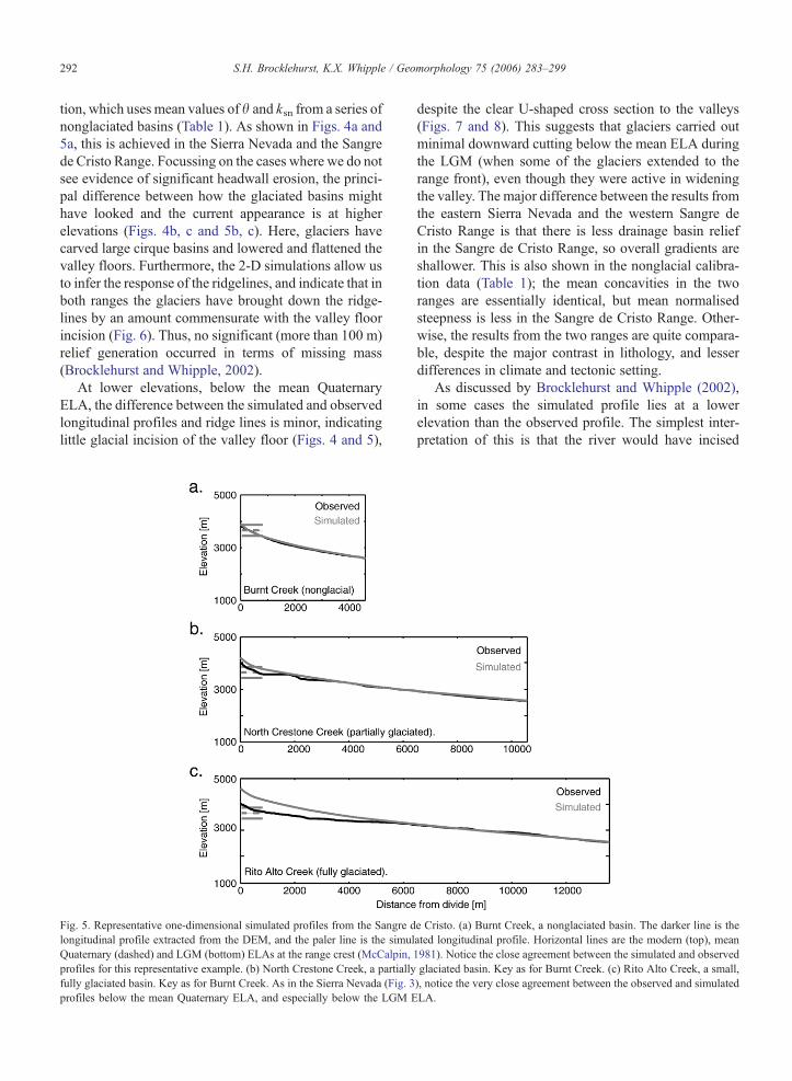
Fig. 5. Representative one-dimensional simulated profiles from the Sangre d
longitudinal profile extracted from the DEM, and the paler line is the simul
Quaternary (dashed) and LGM (bottom) ELAs at the range crest (McCalpin,
profiles for this representative example. (b) North Crestone Creek, a partially
fully glaciated basin. Key as for Burnt Creek. As in the Sierra Nevada (Fig. 3
profiles below the mean Quaternary ELA, and especially below the LGM E
despite the clear U-shaped cross section to the valleys
(Figs. 7 and 8). This suggests that glaciers carried out
minimal downward cutting below the mean ELA during
the LGM (when some of the glaciers extended to the
range front), even though they were active in widening
the valley. The major difference between the results from
the eastern Sierra Nevada and the western Sangre de
Cristo Range is that there is less drainage basin relief
in the Sangre de Cristo Range, so overall gradients are
shallower. This is also shown in the nonglacial calibra-
tion data (Table 1); the mean concavities in the two
ranges are essentially identical, but mean normalised
steepness is less in the Sangre de Cristo Range. Other-
wise, the results from the two ranges are quite compara-
ble, despite the major contrast in lithology, and lesser
differences in climate and tectonic setting.
As discussed by Brocklehurst and Whipple (2002),
in some cases the simulated profile lies at a lower
elevation than the observed profile. The simplest inter-
pretation of this is that the river would have incised
e Cristo. (a) Burnt Creek, a nonglaciated basin. The darker line is the
ated longitudinal profile. Horizontal lines are the modern (top), mean
1981). Notice the close agreement between the simulated and observed
glaciated basin. Key as for Burnt Creek. (c) Rito Alto Creek, a small,
), notice the very close agreement between the observed and simulated
LA.

Fig. 6. Two-dimensional simulations of (a) Independence Creek, Sierra Nevada, and (b) Rito Alto Creek, Sangre de Cristo Range. Longitudinal
profiles drawn from the present topography (black) and simulated topography (pale grey) with the difference between the two in dark grey. Also
shown are the interpolated ridgeline surfaces along the profiles (present topography—black, dashed; simulated topography—pale grey, dashed),
with the relief calculated as the difference in elevation between the interpolated ridgeline and the valley floor (dot-dash lines). ELAs indicated as in
Figs. 3 and 4. Comparing the observed and simulated topography, the valley floor and the ridgeline agree well at lower elevations and then diverge
considerably higher up, with the simulated ridgeline and longitudinal profile considerably higher. We suggest that the valley floor and the ridgelines
have been lowered by glacial erosion.
Fig. 7. 3-D view of shaded relief image draped on topography of
Independence Creek, showing the same extent as the longitudinal
profile (Fig. 3c). The valley floor is wide and flat, and the valley cross
section is U-shaped almost to the basin outlet.
Fig. 8. 3-D view of shaded relief image draped on topography of Rito
Alto Creek, Sangre de Cristo Range.
S.H. Brocklehurst, K.X. Whipple / Geomorphology 75 (2006) 283–299 293
S.H. Brocklehurst, K.X. Whipple / Geomorphology 75 (2006) 283–299294
farther had glaciers not developed upstream. Given that
we have observed several streams in the Sierra Nevada
still flowing over glacially polished bedrock, we doubt
that fluvial erosion outpaces glacial here. Alternatively,
some local complication, such as harder lithology,
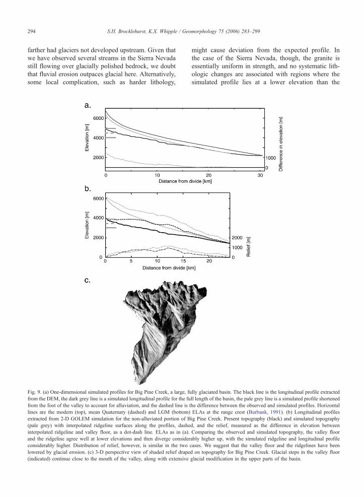
Fig. 9. (a) One-dimensional simulated profiles for Big Pine Creek, a large, fu
from the DEM, the dark grey line is a simulated longitudinal profile for the fu
from the foot of the valley to account for alluviation, and the dashed line is t
lines are the modern (top), mean Quaternary (dashed) and LGM (bottom)
extracted from 2-D GOLEM simulation for the non-alluviated portion of B
(pale grey) with interpolated ridgeline surfaces along the profiles, dashe
interpolated ridgeline and valley floor, as a dot-dash line. ELAs as in (a).
and the ridgeline agree well at lower elevations and then diverge consider
considerably higher. Distribution of relief, however, is similar in the two
lowered by glacial erosion. (c) 3-D perspective view of shaded relief drape
(indicated) continue close to the mouth of the valley, along with extensive
might cause deviation from the expected profile. In
the case of the Sierra Nevada, though, the granite is
essentially uniform in strength, and no systematic lith-
ologic changes are associated with regions where the
simulated profile lies at a lower elevation than the
lly glaciated basin. The black line is the longitudinal profile extracted
ll length of the basin, the pale grey line is a simulated profile shortened
he difference between the observed and simulated profiles. Horizontal
ELAs at the range crest (Burbank, 1991). (b) Longitudinal profiles
ig Pine Creek. Present topography (black) and simulated topography
d, and the relief, measured as the difference in elevation between
Comparing the observed and simulated topography, the valley floor
ably higher up, with the simulated ridgeline and longitudinal profile
cases. We suggest that the valley floor and the ridgelines have been
d on topography for Big Pine Creek. Glacial steps in the valley floor
glacial modification in the upper parts of the basin.

S.H. Brocklehurst, K.X. Whipple / Geomorphology 75 (2006) 283–299 295
observed one. Consequently, our preferred interpreta-
tion is that the glaciers have been responsible for head-
wall retreat/headwater widening (consistent with
patterns of divide migration). This means that our
simulated fluvial profile is too long (and thus has too
great a drainage area) to represent how a never-glaci-
ated profile would look now, so has an overall slope
that is too shallow. Brocklehurst and Whipple (2002)
estimated the magnitude of headwall erosion, in addi-
tion to that which would have occurred under continu-
ous fluvial conditions, by shortening the simulated
profile until a good match was achieved over the
reach where the observed profile has a concave, step-
free shape. In addition to examples from the Sierra
Nevada (Brocklehurst and Whipple, 2002), headwall
erosion is also evident in the Sangre de Cristo Range
(Brocklehurst, 2002).
4.2. Large basins
Fig. 9 illustrates what happens when we extend our
analyses to larger basins, using Big Pine Creek in the
Sierra Nevada as an example, and again using the mean
concavity and normalised steepness values for the east-
ern Sierra Nevada given in Table 1. Attempting to fit
the entire length of the basin produces a 1-D simulated
profile (Fig. 9a) that lies significantly above the ob-
served profile at every point upstream of the outlet. The
simplest interpretation of this is that the glacier here has
incised more rapidly than a river would have done at
every point along the longitudinal profile. We suggest,
however, that this is not quite accurate; the lower
reaches of Big Pine Creek are quite alluviated, and so
trying to simulate an alternative profile with a slope–
area relationship calibrated on bedrock channels is
inappropriate. When we look at only that portion of
the profile with some amount of bedrock in the channel,
as indicated by field observations, we obtain a reason-
able fit to a short section of the profile. Significant
differences from the smaller glaciated basins studied
previously, however, are apparent. Deviation between
the simulated profile and the observed profile occurs far
below the mean Quaternary ELA, even below the LGM
ELA. Here, and also in Bishop Creek, the large glaciers
have incised the valley floor at much lower elevations
than in the smaller basins, even though the glaciers did
not extend much farther beyond the range front (Fig. 1).
As in the smaller glaciated basins, the 2-D simulation
(Fig. 9b) shows that the ridgelines have closely fol-
lowed the response of the longitudinal profile, and,
thus, no major relief production occurred. Fig. 9c illus-
trates, in 3-D, the glacial modification of the longitudi-
nal profile far below the ELA. Although the smaller
basins in the Sierra Nevada show U-shaped cross sec-
tions in the lower part of the basin (Fig. 7), only in the
larger basins is this accompanied by the incision of
dramatic glacial steps.
Fig. 10 illustrates 1-D simulations from the Bubbs
and Palisade Creek tributaries to the Kings River using
mean concavity and normalised steepness values from
the basins listed in Table 1. These simulations highlight
deviations from a smooth, concave longitudinal profile
at several points. Towards the outlet, these may reflect
an alluvial channel. Glacial steps are clearly pronounced
far below the LGM ELA and suggest deep glacial scour
all the way to the LGM terminus. Considering that our
DEM-derived profiles reflect surface elevation rather
than the elevation of bedrock beneath the potentially
deep fills of glacial scours, this is consistent with the
well-known observations of overdeepenings near glacial
termini in Yosemite Valley and the Hetch Hetchy in the
Sierra Nevada (e.g., Gutenberg et al., 1956; MacGregor
et al., 2000), and glaciated basins in the Wind River
Range, Wyoming, and Glacier National Park, Montana.
A component of headwall erosion, particularly in Bubbs
Creek, might also need to be addressed (Brocklehurst
and Whipple, 2002). The scale of the basins on the
western side of the Sierra Nevada, however, means
that we are pushing the limits of what we can learn
using this simulation technique. Calibrating the model
on the western side of the range is hindered by greater
glacial modification of the landscape, making nongla-
ciated basins more elusive. Stepped profiles on the
western side of the range may also reflect lithologic
variations, which are much more pronounced than on
the eastern side of the range (e.g., Wahrhaftig, 1965).
5. Discussion and conclusions
5.1. Summary of results
We have found very similar results applying our
fluvial landscape simulation technique to the eastern
Sierra Nevada and the western Sangre de Cristo Range.
In small drainage basins, glaciers have incised substan-
tially in cirque floors, but ridgelines have also been
lowered, so relief production is minor. Glacial incision
below the mean ELA is also modest, despite obvious
valley widening. The principal difference between the
two ranges is that more total relief occurs in the Sierra
Nevada, so observed and simulated profiles are steeper.
In detail, the two landscapes exhibit subtle differences,
such as lithology exerting an influence on valley
cross-sectional form in the Sangre de Cristo Range
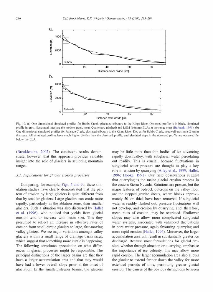
Fig. 10. (a) One-dimensional simulated profiles for Bubbs Creek, glaciated tributary to the Kings River. Observed profile is in black, simulated
profile in grey. Horizontal lines are the modern (top), mean Quaternary (dashed) and LGM (bottom) ELAs at the range crest (Burbank, 1991). (b)
One-dimensional simulated profiles for Palisade Creek, glaciated tributary to the Kings River. Key as for Bubbs Creek; headwall erosion is 2 km in
this case. All simulated profiles have much higher divides than the observed profile, and glaciated steps in the observed profile are observed far
below the ELA.
S.H. Brocklehurst, K.X. Whipple / Geomorphology 75 (2006) 283–299296
(Brocklehurst, 2002). The consistent results demon-
strate, however, that this approach provides valuable
insight into the role of glaciers in sculpting mountain
ranges.
5.2. Implications for glacial erosion processes
Comparing, for example, Figs. 6 and 9b, these sim-
ulation studies have clearly demonstrated that the pat-
tern of erosion by large glaciers is quite different from
that by smaller glaciers. Large glaciers can erode more
rapidly, particularly in the ablation zone, than smaller
glaciers. Such a situation was also discussed by Hallet
et al. (1996), who noticed that yields from glacial
erosion tend to increase with basin size. This they
presumed to reflect an increase in effective rates of
erosion from small cirque glaciers to large, fast-moving
valley glaciers. We see major variations amongst valley
glaciers within a small range of drainage basin sizes,
which suggest that something more subtle is happening.
The following constitutes speculation on what differ-
ences in glacial processes might be responsible. The
principal distinctions of the larger basins are that they
have a larger accumulation area and that they would
have had a lower overall slope prior to the onset of
glaciation. In the smaller, steeper basins, the glaciers
may be little more than thin bodies of ice advancing
rapidly downvalley, with subglacial water percolating
out readily. This is crucial, because fluctuations in
subglacial water pressure are thought to play a key
role in erosion by quarrying (Alley et al., 1999; Hallet,
1996; Hooke, 1991). Our field observations suggest
that quarrying is the major glacial erosion process in
the eastern Sierra Nevada. Striations are present, but the
major features of bedrock outcrops on the valley floor
are the stepped granite sheets, where blocks approxi-
mately 50 cm thick have been removed. If subglacial
water is readily flushed out, pressure fluctuations will
not develop, and erosion by quarrying, and, therefore,
mean rates of erosion, may be restricted. Shallower
slopes may also allow more complicated subglacial
water systems, associated with enhanced fluctuations
in pore water pressure, again favouring quarrying and
more rapid erosion (Hallet, 1996). Moreover, the larger
accumulation area will result in substantially greater ice
discharge. Because most formulations for glacial ero-
sion, whether through abrasion or quarrying, emphasise
the importance of ice velocity, this may allow more
rapid erosion. The larger accumulation area also allows
the glacier to extend farther down the valley for more
extended periods of time, permitting greater glacial
erosion. The causes of the obvious distinctions between

S.H. Brocklehurst, K.X. Whipple / Geomorphology 75 (2006) 283–299 297
small basins, normally occupied by modest cirque gla-
ciers, and large drainages featuring larger valley gla-
ciers represent an important focus for future research.
A final question of the dynamics of glacial erosion is
why the smaller glaciers widen the valley floor without
incising. As demonstrated by Harbor (1992), starting
from an initial V-shaped cross section, erosion driven
by ice velocity will be focussed initially towards the
development of a U-shaped cross section. It is possible
that, because of the short residence times of these
glaciers at the full LGM extents (Porter, 1989), the
glaciers have not yet been able to pass out of this
stage. We suggest that subglacial water may again
play a crucial role. The subglacial water along the
steep thalweg is likely to form a well-connected net-
work for much of the annual cycle and reduce the
possibility of large fluctuations in water pressure (Hal-
let, 1996; Hooke, 1991). Along the glacier margins, the
subglacial drainage network may not be as well devel-
oped, while crevasses will allow meltwater to percolate
to the base, potentially allowing greater water pressure
fluctuations, and, thus, more rapid erosion. Meanwhile,
as described above, larger glaciers may be more capable
of incision along the thalweg along with valley widen-
ing. We, thus, highlight the role of subglacial water in
erosion processes as a key focus for future research.
This study suggests that a range of possible
responses exists for glacial erosion systems of different
scales. Initial efforts on constructing evolution models
for the glacial landscape have focussed on the larger
scale end of the spectrum (Braun et al., 1999; MacGre-
gor et al., 2000; Merrand and Hallet, 2000; Oerlemans,
1984). Predictions of these models include large over-
deepenings below the long-term ELA, in addition to
overdeepenings associated with tributary junctions.
Further development of these models, to capture the
full diversity of glacial landscapes, will lead to a more
complete understanding of glacial erosion.
5.3. Limitations and future applications of the
technique
The principal limitation on comparing fluvial land-
scapes with observed glacial landscapes to deduce the
effects of glacial erosion on a mountain belt is the
requirement that the fluvial landscapes must be in
close proximity to the glacial ones. This stems from a
current inability to precisely predict parameters in flu-
vial erosion formulations based purely on a set of
climatic, tectonic and lithologic observations. Only at
higher latitudes have glaciers sculpted every basin
within a mountain range. The work presented here
has demonstrated the applicability of our approach in
two ranges with different lithologies and somewhat
different climates and tectonic settings.
This analysis exploits the fact that we understand the
characteristics of fluvial landscapes better than glaciat-
ed landscapes. As yet we are unable to use this ap-
proach to establish convincingly how the range might
have looked prior to glaciation, because of (i) uncer-
tainty over how h and ks respond to climate change
(e.g., Roe et al., 2002; Whipple et al., 1999); and (ii)
lack of detailed understanding of the base-level history
over the Quaternary (for instance, how the Owens
Valley fell with respect to the Sierra Nevada (Gillespie,
1982), and how the San Luis Valley fell with respect to
the Sangre de Cristo Range (e.g., McCalpin, 1981)).
Understanding the response of rivers to climate change
during the Quaternary would allow us to predict how
mountain ranges would have looked prior to the onset
of glaciation, while the ability to constrain model para-
meters of erosion purely on the basis of climatic, tec-
tonic and lithologic parameters would allow application
of this approach where local calibration of the fluvial
erosion model is not possible.
The application of a single calibration leads to pro-
blems when the valley floor encompasses alluvial and
bedrock reaches. This can be solved in larger basins,
where alluviation is a natural consequence of steadily
increasing drainage area, by restricting the analysis to
the bedrock portions of the profile. Where a small
stream is choked by debris from the last glaciation, as
in the eastern Sangre de Cristo Range, however, a
realistic model fit is not possible because of the close
proximity of the morainal debris, occasional bedrock
reaches, and the glacially modified upper section. Ac-
cordingly, the analysis was restricted to the western side
of the Sangre de Cristo Range.
If fluvial and glacial basins with similar tectonics
and precipitation can be found, this approach would
allow us to compare the responses of rivers and glaciers
to rapid tectonic uplift, for example in the Southern
Alps of New Zealand. Preliminary results using this
approach in the Manaslu region of the Himalayas
(Whipple and Brocklehurst, 2000) emphasised the abil-
ity of glaciers to maintain a shallow gradient in spite of
rapid uplift, unlike their fluvial counterparts (Brockle-
hurst, 2002; Brozovic et al., 1997).
Acknowledgements
This work was supported by NSF Grant EAR-
9980465 (to KXW), a NASA Graduate Fellowship, a
GSA Fahnestock Award, and a CIRES Visiting Fellow-

S.H. Brocklehurst, K.X. Whipple / Geomorphology 75 (2006) 283–299298
ship (all to SHB). Thorough, constructive reviews by
Eric Leonard and an anonymous reviewer helped great-
ly to clarify the manuscript.
References
Alley, R.B., Strasser, J.C., Lawson, D.E., Evenson, E.B., Larson, G.J.,
1999. Glaciological and geological implications of basal-ice ac-
cretion in overdeepenings. In: Mickelson, D.M., Attig, J.W.
(Eds.), Glacial Processes Past and Present, Geological Society
of America Special Paper. Geological Society of America, Boul-
der, Colorado, pp. 1–9.
Baldwin, J.A., Whipple, K.X., Tucker, G.E., 2003. Implications of the
shear-stress river incision model for the timescale of post-orogenic
decay of topography. Journal of Geophysical Research 108 (B3).
doi:10.1029/2001JB000550.
Bateman, P.C., 1965. Geology and tungsten mineralization of the
bishop district, California. U.S. Geological Survey Professional
Paper 470 (208 pp.).
Braun, J., Zwartz, D., Tomkin, J.H., 1999. A new surface-processes
model combining glacial and fluvial erosion. Annals of Glaciol-
ogy 28, 282–290.
Brocklehurst, S.H., (2002). Evolution of Topography in Glaciated
Mountain Ranges. PhD Thesis, Massachusetts Institute of Tech-
nology, Cambridge, MA. 236 pp.
Brocklehurst, S.H., Whipple, K.X., 2002. Glacial erosion and relief
production in the eastern Sierra Nevada, California. Geomorphol-
ogy 42 (1–2), 1–24.
Brozovic, N., Burbank, D.W., Meigs, A.J., 1997. Climatic limits on
landscape development in the northwestern Himalaya. Science
276, 571–574.
Burbank, D.W., 1991. Late quaternary snowline reconstructions for
the southern and central Sierra Nevada, California and a reassess-
ment of the brecess peak glaciationQ. Quaternary Research 36,
294–306.
Flint, J.J., 1974. Stream gradient as a function of order, magnitude,
and discharge. Water Resources Research 10, 969–973.
Gillespie, A.R., 1982. Quaternary Glaciation and Tectonism in the
Southeastern Sierra Nevada, Inyo County, California. PhD Thesis,
California Institute of Technology, Pasadena. 695 pp.
Gutenberg, B., Buwalda, J.P., Sharp, R.P., 1956. Seismic explorations
on the floor of Yosemite Valley, California. Geological Society of
America Bulletin 67, 1051–1078.
Hack, J.T., 1957. Studies of longitudinal stream profiles in Virginia
and Maryland. U.S. Geological Survey Professional Paper 294-B,
97.
Hallet, B., 1996. Glacial quarrying: a simple theoretical model. An-
nals of Glaciology 22, 1–8.
Hallet, B., Hunter, L., Bogen, J., 1996. Rates of erosion and sediment
evacuation by glaciers: a review of field data and their implica-
tions. Global and Planetary Change 12, 213–235.
Harbor, J.M., 1992. Numerical modeling of the development of U-
shaped valleys by glacial erosion. Geological Society of America
Bulletin 104, 1364–1375.
Hicks, D.M., McSaveney, M.J., Chinn, T.J.H., 1990. Sedimentation in
proglacial Ivory lake, Southern Alps, New Zealand. Arctic and
Alpine Research 22, 26–42.
Hooke, R.L., 1991. Positive feedbacks associated with erosion of
glacial cirques and overdeepenings. Geological Society of Amer-
ica Bulletin 103, 1104–1108.
Howard, A.D., Dietrich, W.E., Seidl, M.A., 1994. Modeling fluvial
erosion on regional to continental scales. Journal of Geophysical
Research 99, 13971–13986.
Huber, N.K., 1981. Amount and timing of late Cenozoic uplift and tilt
of the central Sierra Nevada, California—evidence from the upper
San Joaquin river. U.S. Geological Survey Professional Paper
1197 (28 pp.).
Johnson, B.R, Lindsey, D.A. Bruce, R.M., Soulliere, S.J., 1987.
Reconnaissance geologic map of the Sangre de Cristo Wilderness
Study Area, south-central Colorado. USGS Miscellaneous Field
Studies Map, MF-1635-B.
Koppes, M.N., Hallet, B., 2002. Influence of rapid glacial retreat on
the rate of erosion by tidewater glaciers. Geology 30 (1), 47–50.
Le, K., 2004. Late Pleistocene to Holocene extension along the Sierra
Nevada range front fault zone, California. MSc thesis Thesis,
Central Washington University.
Leopold, L.B., Wolman, M.G., Miller, J.P., 1964. Fluvial Processes in
Geomorphology. W.H. Freeman, San Francisco. 522 pp.
McCalpin, J.P., 1981. Quaternary geology and neotectonics of the
west flank of the northern Sangre de Cristo Mountains, south-
central Colorado. Doctoral Thesis, Colorado School of Mines,
Golden, CO. 287 pp.
McCalpin, J.P., 1986. Quaternary tectonics of the Sangre de Cristo
and villa grove fault zones. Special Publication - Colorado Geo-
logical Survey 28, 59–64.
McCalpin, J.P., 1987. Recurrent quaternary normal faulting at major
creek, Colorado: an example of youthful tectonism on the eastern
boundary of the Rio Grande rift zone. In: Beus, S.S. (Ed.),
Geological Society of America Centennial Field Guide—Rocky
Mountain Section. Geological Society of America, pp. 353–356.
MacGregor, K.C., Anderson, R.S., Anderson, S.P., Waddington, E.D.,
2000. Numerical simulations of glacial valley longitudinal profile
evolution. Geology 28 (11), 1031–1034.
Merrand, Y., Hallet, B., 2000. A physically based numerical model of
orogen-scale glacial erosion: importance of subglacial hydrology
and basal stress regime. GSA Abstracts with Programs 32 (7),
A329.
Molnar, P., England, P., 1990. Late Cenozoic uplift of mountain
ranges and global climate change: chicken or egg? Nature 346,
29–34.
Montgomery, D.R., Foufoula-Georgiou, E., 1993. Channel network
source representation using digital elevation models. Water
Resources Research 29 (12), 3925–3934.
Montgomery, D.R., Balco, G., Willett, S.D., 2001. Climate, tectonics
and the morphology of the Andes. Geology 29 (7), 579–582.
Moore, J.G., 1963. Geology of the mount Pinchot quadrangle, south-
ern Sierra Nevada, California. US Geological Survey Bulletin
1130 (152 pp.).
Moore, J.G., 1981. Geologic map of the Mount Whitney quadrangle,
Inyo and Tulare Counties, California, GQ-1545. US Geological
Survey Map.
Oerlemans, J., 1984. Numerical experiments on large-scale glacial
erosion. Zeitschrift fuer Gletscherkunde und Glazialgeologie 20,
107–126.
Oskin, M., Burbank, D.W., 2002. Geomorphic evolution of steady-
state in a glaciated mountain range: kyrgyz range, Western Tien
Shan. Eos, Transactions of the American Geophysical Union 83
(47), F1325.
Paterson, W.S.B., 1994. The Physics of Glaciers. Pergamon, Oxford,
OX, England. ix, 480 pp.
Porter, S.C., 1989. Some geological implications of average quater-
nary glacial conditions. Quaternary Research 32, 245–261.
S.H. Brocklehurst, K.X. Whipple / Geomorphology 75 (2006) 283–299 299
Raymo, M.E., Ruddiman, W.F., 1992. Tectonic forcing of late Ceno-
zoic climate. Nature 359, 117–122.
Raymo, M.E., Ruddiman, W.F., Froelich, P.N., 1988. Influence of late
Cenozoic mountain building on ocean geochemical cycles. Geol-
ogy 16, 649–653.
Roe, G.H., Montgomery, D.R., Hallet, B., 2002. Effects of orographic
precipitation variations on the concavity of steady-state river
profiles. Geology 30 (2), 143–146.
Snyder, N.P., Whipple, K.X., Tucker, G.E., Merritts, D.J., 2000. Land-
scape response to tectonic forcing: DEM analysis of stream profiles
in the Mendocino triple junction region, northern California. Geo-
logical Society of America Bulletin 112 (8), 1250–1263.
Stock, J., Dietrich, W.E., 2003. Valley incision by debris flows:
evidence of a topographic signature. Water Resources Research
39 (4). doi:10.1029/2001WR001057.
Stone, P., Dunne, G.C., Moore, J.G., Smith, G.I., 2001. Geologic Map
of the Lone Pine 15’ Quadrangle, Inyo County, California. U.S.
Geological Survey Geologic Investigations Series, I-2617: Online
version 1.0.
Tarboton, D.G., Bras, R.L., Rodriguez-Iturbe, I., 1991. On the ex-
traction of channel networks from digital elevation data. Hydro-
logical Processes 5, 81–100.
Tomkin, J.H., Braun, J., 2002. The influence of alpine glaciation on
the relief of tectonically active mountain belts. American Journal
of Science 302, 169–190.
Tucker, G.E., Slingerland, R.L., 1994. Erosional dynamics, flexural
isostasy, and long-lived escarpments: a numerical modeling study.
Journal of Geophysical Research 99 (B6), 12229–12243.
Tucker, G.E., Slingerland, R.L., 1997. Drainage basin responses to
climate change. Water Resources Research 33, 2031–2047.
Wahrhaftig, C., 1965. Stepped topography of the Southern Sierra
Nevada, California. Geological Society of America Bulletin 76,
1165–1190.
Wakabayashi, J., Sawyer, T.L., 2001. Stream incision, tectonics,
uplift, and evolution of topography of the Sierra Nevada, Cali-
fornia. Journal of Geology 109, 539–562.
Wettlaufer, J.S., 2001. Dynamics of snow and ice masses. Lecture
Notes in Physics 582, 211–217.
Whipple, K.X., Brocklehurst, S.H., 2000. Estimating glacial relief
production in the Nepal Himalaya. GSA Abstracts with Programs
32, A320.
Whipple, K.X., Trayler, C.R., 1996. Tectonic control of fan size: the
importance of spatially variable subsidence rates. Basin Research
8, 351–366.
Whipple, K.X., Tucker, G.E., 1999. Dynamics of the stream-power
river incision model: implications for height limits of mountain
ranges, landscape response timescales, and research needs. Jour-
nal of Geophysical Research 104, 17661–17674.
Whipple, K.X., Kirby, E., Brocklehurst, S.H., 1999. Geomorphic
limits to climate-induced increases in topographic relief. Nature
401, 39–43.
Willgoose, G., 1994. A statistic for testing the elevation characteristics
of landscape simulation models. Journal of Geophysical Research
99 (B7), 13987–13996.
Wobus, C. et al., in press. Tectonics from topography: Procedures,
promise and pitfalls. In: S.D. Willett, N. Hovius, M. Brandon, D.
Fisher (Eds.), GSA Penrose Special Paper: Tectonics, Climate and
Landscape Evolution.