Ateneo de Manila University Ateneo de Manila University

Archīum Ateneo Arch um Ateneo

Physics Faculty Publications Physics Department

2017

Assessing the optimized precision of the aircraft mass balance Assessing the optimized precision of the aircraft mass balance

method for measurement of urban greenhouse gas emission method for measurement of urban greenhouse gas emission

rates through averaging rates through averaging

Alexie M F Heimburger

Rebecca M. Harvey

Paul B. Shepson

Brian H. Stirm

Chloe Gore

See next page for additional authors

Follow this and additional works at: https://archium.ateneo.edu/physics-faculty-pubs

Part of the Atmospheric Sciences Commons

Authors Authors Alexie M F Heimburger, Rebecca M. Harvey, Paul B. Shepson, Brian H. Stirm, Chloe Gore, Jocelyn Turnbull, Maria Obiminda L. Cambaliza, Olivia E. Salmon, Anna-Elodie M. Kerlo, Tegan Lavoie, Kenneth J. Davis, Thomas Lauvaux, Anna Karion, Colm Sweeney, W Alan Brewer, R Michael Hardesty, and Kevin R. Gurney

Heimburger, AMF, et al 2017 Assessing the optimized precision of the aircraft mass balance method for measurement of urban greenhouse gas emission rates through averaging. Elem Sci Anth, 5: 26, DOI: https://doi.org/10.1525/elementa.134

1. Introduction Urban greenhouse gas emissions, as well as city expansion, are expected to continue to grow in the coming years (IEA, 2008; Seto et al., 2012). Currently, fossil fuel-related carbon dioxide (CO2) emissions from cities represent more than

70% of the global total, mainly due to energy production and use (IEA, 2008; IPCC 5th Assessment Report, 2014), which also represents the second major anthropogenic source of carbon monoxide (CO) after biomass burn-ing (Olivier et al., 1996). Recent studies have shown that

RESEARCH ARTICLE

Assessing the optimized precision of the aircraft mass balance method for measurement of urban greenhouse gas emission rates through averagingAlexie M. F. Heimburger*, Rebecca M. Harvey*, Paul B. Shepson*,†, Brian H. Stirm‡, Chloe Gore*, Jocelyn Turnbull§, Maria O. L. Cambaliza‖, Olivia E. Salmon*, Anna-Elodie M. Kerlo*, Tegan N. Lavoie*, Kenneth J. Davis¶, Thomas Lauvaux¶, Anna Karion**,††,§§, Colm Sweeney**,††, W. Allen Brewer**, R. Michael Hardesty†† and Kevin R. Gurney‡‡

To effectively address climate change, aggressive mitigation policies need to be implemented to reduce greenhouse gas emissions. Anthropogenic carbon emissions are mostly generated from urban environments, where human activities are spatially concentrated. Improvements in uncertainty determinations and precision of measurement techniques are critical to permit accurate and precise tracking of emissions changes relative to the reduction targets. As part of the INFLUX project, we quantified carbon dioxide (CO2), carbon monoxide (CO) and methane (CH4) emission rates for the city of Indianapolis by averaging results from nine aircraft-based mass balance experiments performed in November-December 2014. Our goal was to assess the achievable precision of the aircraft-based mass balance method through averaging, assuming constant CO2, CH4 and CO emissions during a three-week field campaign in late fall. The averaging method leads to an emission rate of 14,600 mol/s for CO2, assumed to be largely fossil-derived for this period of the year, and 108 mol/s for CO. The relative standard error of the mean is 17% and 16%, for CO2 and CO, respectively, at the 95% confidence level (CL), i.e. a more than 2-fold improvement from the previous estimate of ~40% for single-flight measurements for Indianapolis. For CH4, the averaged emission rate is 67 mol/s, while the standard error of the mean at 95% CL is large, i.e. ±60%. Given the results for CO2 and CO for the same flight data, we conclude that this much larger scatter in the observed CH4 emission rate is most likely due to variability of CH4 emissions, suggesting that the assumption of constant daily emissions is not correct for CH4 sources. This work shows that repeated measurements using aircraft-based mass balance methods can yield sufficient precision of the mean to inform emissions reduction efforts by detecting changes over time in urban emissions.

Keywords: greenhouse gas; emission rates; precision; urban; quantification

* Department of Chemistry, Purdue University, West Lafayette, Indiana, US

† Department of Earth, Atmospheric and Planetary Science and Purdue Climate Change Research Center, Purdue University, West Lafayette, Indiana, US

‡ Department of Aviation and Transportation Technology, Purdue University, West Lafayette, Indiana, US

§ National Isotope Center, GNS Science, Lower Hutt, NZ‖ Department of Physics, Ateneo de Manila University, Loyola Heights, Quezon City, PH

¶ The Pennsylvania State University, Department of Meteorology, University Park, PA

** NOAA/ESRL, Colorado, US†† CIRES, University of Colorado at Boulder, Boulder, Colorado, US‡‡ School of Life Sciences, Arizona State University, Tempe, Arizona, US

§§ NIST, Gaithersburg, Maryland, USCorresponding author: Alexie M. F. Heimburger (alexie.heimburger@gmail.com)

Heimburger et al: Assessing the optimized precision of the aircraft mass balance method for measurement of urban greenhouse gas emission rates through averaging

Art. 26, page 2 of 15

urban environments also emit large amounts of methane (CH4) (Wunch et al., 2009, Wennberg et al., 2012, McKain et al., 2015), a potent greenhouse gas (GHG) with a global warming potential 28–34 times greater than that of CO2 over a 100-year time period (Myhre et al., 2013). Despite ocean and land sinks, ~55% of CO2 emissions accumulate in the atmosphere and can thus impact the global climate (Kirschke et al., 2013; Le Quéré et al., 2014). Quantification of both the magnitude and uncertainty of GHG emissions in urban environments is therefore critical for imple-menting coherent and effective policies to mitigate such emissions, and to reduce their effects on climate change (IEA, 2008; Hutyra et al., 2014).

Since the Copenhagen Accord in 2009, several countries have confirmed their commitment to reduce their GHG emissions (UNFCCC, 2010; President’s Climate Action Plan, 2013, 2014a, 2014b; European Commission, 2014). During the recent United Nations Framework Convention on Climate Change negotiating session held in Paris 2015 (COP21/CMP11), the United States announced a goal of 26–28% reduction in emissions by 2025 com-pared to 2005 levels, while China committed to a carbon dioxide emissions reduction of 60–65% per unit of gross domestic product by 2030 (China’s INDC, June 2015). Europe adopted a reduction target of at least 40% below 1990 levels by 2030 (30–40% below 2005 depending on activity sectors; http://ec.europa.eu/clima/policies/strat-egies/2030/index_en.htm, accessed on 12/07/2015). Such goals are achievable, but reduction efforts need to be “measurable”, “reportable”, and “verifiable” (Vine and Sathaye, 1999; Schakenbach et al., 2006; NRC, 2010; UNFCCC, 2015). Measurements of GHG emissions often have significant uncertainties, ranging from less than 10% to 100% (NRC, 2010), depending on the methods used (e.g., bottom-up inventories, which assess and integrate emissions from specific sources and activities; top-down techniques, which rely on greenhouse gas concentration measurements conducted within the atmosphere), the type of sources and target gases, and the spatial scale considered (national, regional, and local) (Marland, 2008, 2012; NRC, 2010; Peylin et al., 2011; Kirschke et al., 2013; Cambaliza et al., 2014; Bergamaschi et al., 2015). Uncertainties for GHG emissions at sub-national scales (e.g. city/county/state/province) are usually significantly greater (~50% to >100%, Gurney et al., 2009; Mays et al., 2009; NRC, 2010; Cambaliza et al., 2014; 2015) than those at national or continental scales (< 25% at national levels, Marland, 2008, 2012; Gurney et al., 2009; NRC, 2010), and are in many cases larger than the emission reduction targets themselves, making it difficult to assess the efficacy of local scale efforts. These large uncertainties can be par-tially explained by the dearth of local-scale measurements and method development, coupled with the general lack of local-scale mitigation efforts (Rosenzweig et al., 2010; Hutyra et al., 2014). However, local policy plans initiated by proactive cities and networks of local political decision-makers (i.e. World Mayors Council on Climate Change, Local Governments for Sustainability) have recently emerged and highlighted the urgent need of new and timely information on urban GHG emissions from the

scientific community (Rosenzweig et al., 2010; Hutyra et al., 2014).

Urban emissions of CO2, CH4, and CO (a proxy for combustion) are usually derived from several natural and anthropogenic sources that are difficult to separate (Hutyra et al., 2014). Both fossil fuel- and biogenic-related CO2 con-centrations in urban environments are affected by many sources and sinks. Fossil fuel-related CO2 is largely emitted by electricity generation, mobile source combustion, and point sources, such as large industrial facilities. Biogenic CO2 sources and sinks include biosphere respiration, biofuel use, and biomass burning. CO has been used as a tracer for anthropogenic sources (Parrish et al., 1993; Turbull et al., 2011), and is emitted during incomplete com-bustion of fossil- and bio-fuels from vehicles, agricultural waste (not at Indianapolis), and industrial processes. CO is also produced by oxidation of biogenic volatile carbon compounds, especially during the summer time, and is consumed in the atmosphere by reaction with the OH radi-cal (Parrish et al., 1993). CH4 can be emitted from natural wetlands, or from anthropogenic sources (Bousquet et al., 2006; Kirschke et al., 2013), such as rice production (not at Indianapolis), ruminant animals (not at Indianapolis), natural gas infrastructure, biomass burning, landfills, and wastewater treatment plants. CH4 emission estimates are usually less certain than CO2 estimates because many CH4 sources are more diffuse, as a result of unintended release or more complex and temporally and spatially variable biological decay processes (Forster et al., 2007; Kirschke et al., 2013; President’s Climate Action Plan, 2014b).

Improvement in the quality of GHG measurements represents an urgent challenge. The development of low cost, precise emissions measurement techniques that can be applied to a range of urban environments is needed to provide scientifically sound information for future GHG mitigation strategies, whether local, regional or national. The multi-institution collaborative Indianapolis Flux Experiment project (INFLUX, http://sites.psu.edu/influx/) was designed to evaluate and minimize GHG emis-sions uncertainties at the city-scale, by developing, assess-ing, combining, and improving top-down and bottom-up approaches to quantify urban GHG emissions. Indianapolis is an advantageous test area, due to its physical separation from adjacent cities by surrounding agricultural lands, effectively isolating the city from other major sources of anthropogenic pollution (Cambaliza et al., 2014, 2015). The INFLUX project involves various top-down approaches to estimate CO2, CH4, and CO emissions from the city using continuous measurements and flask sampling from 12 towers situated within the city and in the surround-ing suburbs (Miles et al., 2015; Turnbull et al., 2012, 2015), periodic aircraft measurements (Mays et al., 2009; Cambaliza et al., 2014, 2015), inverse modeling (Lauvaux et al., 2016), and a high resolution model-data fusion product, Hestia, providing a bottom-up estimate of fossil fuel-related CO2 emissions for Indianapolis (Gurney et al., 2012). Integration of multiple top-down and bottom-up approaches are needed to converge on the most accurate, policy-relevant, and mechanistically representative emis-sion estimate (Nisbet and Weiss, 2010).

Heimburger et al: Assessing the optimized precision of the aircraft mass balance method for measurement of urban greenhouse gas emission rates through averaging

Art. 26, page 3 of 15

As part of INFLUX, we have been quantifying the emis-sion rates for CO2 and CH4 for the city of Indianapolis since 2008, and for CO since 2014, using a top-down aircraft-based mass balance approach. Top-down aircraft-based approaches are particularly effective at quantifying urban emissions because of their capability to sample the entire plume of a large emission source, with a short deployment time. Limitations of this method of measurement include initial costs, sporadic frequency of measurements, reliance on weather conditions (e.g. constant wind direction), and challenges in the definition of background conditions (e.g. White et al., 1976; Trainer et al., 1995; Lind and Kok, 1999; Kalthoff et al., 2002; Carras et al., 2002; Mays et al., 2009; Turnbull et al., 2011; O’Shea et al., 2014a, 2014b; Gioli et al., 2014; Cambaliza et al., 2014, 2015; Karion et al., 2015). However, aircraft-based measurement approaches have been successfully com-pared to bottom-up inventories (Cambaliza et al., 2014; Karion et al., 2015; Lamb et al., 2016). While accurate aver-age results are achievable, individual flight realizations of emission rates have an uncertainty of ~ ±40% (Cambaliza et al., 2014).

In this paper, we describe our efforts to evaluate the potential of the mass balance experiment (MBE) approach to achieve useful precision through averaging of assumed random error. Karion et al. (2015) showed that, by averag-ing eight flight experiments, the precision of the mean for the MBE approach can be significantly improved when data are collected in a relatively short period of time, enabling the assumption of constant GHG emis-sions during the sampling period. They demonstrated that the averaged CH4 emission rate in the Barnett Shale region, which includes eight different counties with dense natural gas production and urban areas, can be known with a precision of ~28% using the 1-sigma standard deviation of the mean, and of 17% at the 95% confidence level (CL) using a statistical bootstrapping method, while the relative uncertainties they found for a single-flight MBE can be as high as ~40%. In this paper, we investi-gate the efficacy of this method at the city scale through averaging of nine MBEs conducted from November 13th to December 3rd 2014 (3 weeks). We present and discuss the results for CO2, CO, and CH4 emission rates for the nine MBEs, and their average and standard error of the mean at 95% CL. Finally, we discuss the variability of the emission rates, and areas for improvement of this method.

2. Methods2.1 Study areaIndianapolis, Indiana (39.79°N, 86.15°W, ~240 m above sea level) is the 12th largest city in the United States with a population of 848,800 (2014 United States Census Bureau) (Figure 1). The metropolitan area, combin-ing Indianapolis, Carmel and Anderson, has (for the study period) a population of 1,971,000. Indianapolis is located on a flat plain, at least 120 km away from other metropolitan areas and is surrounded in all directions by rural land-use, primarily cropland. This isolated urban geography, often referred to as an “island city”, is also accompanied by a relatively uniform inflow of boundary

layer GHG concentrations, since upwind anthropogenic sources are relatively well-mixed when they reach Indianapolis (Cambaliza et al., 2014). These features make atmospheric measurements easier to interpret and simulate.

2.2 Aircraft instrumentationCH4, CO, and CO2 emissions were quantified using an aircraft-based platform, combined with a mass balance approach. Flight experiments were performed using Purdue University’s Airborne Laboratory for Atmospheric Research (ALAR, http://science.purdue.edu/shepson/research/bai/alar.html), a light twin-engine Beechcraft Duchess aircraft with an instrumentation compartment space of ~1 m3. This aircraft is equipped with i) a global positioning and inertial navigation system (GPS/INS), ii) a Best Air Turbulence (BAT) probe for wind measurements (Crawford and Dobosy, 1992; Garman et al. 2006, 2008), iii) a Picarro cavity ring-down spectrometer (CRDS, model G2401-m) for in-situ, real-time CO2, CO, CH4, and H2O measurements (Crosson, 2008; see Karion et al. (2013a) for more details on the instrument performance), iv) an in-flight CO2/CH4 calibration system, and v) a program-mable flask package (PFP) system for discrete ambient air sampling (Karion et al., 2013a; Sweeney et al., 2015).

Wind speeds and wind directions were obtained at 50 Hz using data from the nine-port differential pres-sure BAT probe that extends from the nose of the aircraft. Atmospheric temperature was measured using a micro-bead thermistor located at the center of the probe. A fast response thermocouple was also attached to the probe for comparison with the microbead observations. The measured pressure variations across the hemisphere of the probe were combined with 50 Hz spatial data from both GPS/INS and temperature sensors to obtain the three-dimensional wind vectors (Garman et al, 2006).

The CRDS measures gas concentrations at 0.5 Hz. Ambient air is pulled from the nose of the aircraft through a 5 cm diameter PFA Teflon tube at a flow rate of 1840 l/min (resi-dence time: ~0.1 s) using a high-capacity blower located at the rear of the aircraft. The spectrometer is connected to the Teflon tubing using a tee and a 0.64 cm diameter Teflon inlet line, allowing ambient air to be continuously pumped through the analyzer at a flow rate of ~300 sccm (residence time: ~10 s). Just before the beginning and at the end of each MBE, both CO2 and CH4 were calibrated in-flight using three NOAA/ESRL reference cylinders. The certified mole fractions in each tank were: i) low concentrations: 368.02 ppm and 1781.05 ppb for CO2 and CH4, respectively, ii) medium concentrations: 410.73 ppm and 2222.42 ppb, iii) high concentrations: 447.11 ppm and 3261.49 ppb. The NOAA reproducibility (1 s) on the cylinder measurements are 0.03 ppm for CO2 and 0.35 ppb for CH4. The CRDS exhibits consistent reproducibility and linearity over time (Supplementary information: Figure S1). CO was calibrated at NOAA/ESLR before and after the field campaign, i.e. in Sept. 2014 and July 2015. The two calibrations exhibited the same calibration coefficients to within the uncertainty of the measurement, which was determined using in-flight calibrations, as described in Section S1.

Heimburger et al: Assessing the optimized precision of the aircraft mass balance method for measurement of urban greenhouse gas emission rates through averaging

Art. 26, page 4 of 15

2.3 Flight design and boundary layer height determinationNine MBEs were performed during the late fall, on week-days, from Nov. 13th to Dec. 3rd 2014 (Table S1). They were conducted when the convective boundary layer (CBL) was most likely fully developed and relatively constant in height throughout the duration of the experiment (about 4 hours on average), i.e. between 12:00 and 16:00 local time (Cambaliza et al., 2014). Prior to each flight, we ensured that morning wind conditions were sufficiently strong (wind speed at the surface and aloft) and consistent (wind direction) to avoid significant GHG accumulation in the boundary layer prior to our measurements (wind condi-tions monitored via Forecast (http://www.wunderground.com/, Terminal Aerodrome Forecast/TAF, Model Output Statistics/MOS) and real time weather at Indianapolis Auto-matic Weather Observation System/ASOS, METeorological Airport Report/METAR). For a typical MBE, the aircraft groundtrack was oriented perpendicular to the wind direction to intercept the polluted plume from the city (e.g. Carras et al., 2002). Three to five horizontal transects were performed at one downwind distance from the city and at different constant altitudes up to close to the top of the CBL (zi) (Figure 1, Figure S2). Downwind transects were flown approximately 30 km from the city center, a distance far enough from the city that the plume was well-mixed but close enough to measure the urban plume above the background and to minimize mixing to and contact with the top of the boundary layer. The downwind transects allow for the construction of a two-dimensional plane onto which measurements are projected (e.g. Carras

et al. 2002; Kalthoff et al., 2002; Cambaliza et al., 2014). Indianapolis is approximately 70 km in width and there-fore transect lengths are extended to 80–100 km to allow the capture of downwind air from beyond the city limits for regional background concentration determination ( Cambaliza et al., 2014). One upwind horizontal transect (30 km upwind of the city center) was flown at a constant altitude (approximately 350 m above ground, Figure S2) prior to the downwind transects to identify possible sig-nificant CO, CO2, and CH4 sources upwind of Indianapolis, which would contribute to the observed city plume. In this case and since only one upwind transect is performed by MBE, the emission rate of the upwind point source was calculated by a single transect approach (Turnbull et al., 2011; Karion et al., 2013b). The emission rate is then sub-tracted from the final downwind emission rate exiting the city. A significant upwind source of CO2 from the Eagle Valley power plant was transported to the city on Nov. 19th, the only day where upwind CO2 emissions were observed (Figure S2). No identifiable upwind CO emissions were observed during the field campaign. Depending on the wind direction, CH4 emissions from two different land-fills located outside the city are evident in the sampled air and thus mixed into the city plume (TwinBridges if westerly winds, Caldwell if easterly winds, see Figures 1 and S2). We subtracted the averaged emission rate of the respective landfill reported in Cambaliza et al. (2017), when necessary. Specifically, we subtracted an emission rate of 12.2 mol/s estimated for the TwinBridges landfill ( Cambaliza et al., 2017) from the city-wide CH4 emission rate obtained on Nov. 13th, 14th, 17th, 19th, 20th, 25th and

Figure 1: Flight path on December 01, 2014. Example of flight path (Dec 01 2014) performed over Indianapolis for the November-December field campaign, comprising two vertical profiles at the beginning and end of the experiment (VP1 and VP2, respectively), one upwind transect and several downwind transects flown at one downwind distance and different altitudes. DOI: https://doi.org/10.1525/elementa.134.f1

Abbreviations used in figure legend: PP: power plant, LF: landfill, WWTP: wastewater treatment plant, Towers: loca-tion of INFLUX towers, TRS: natural gas transmission regulating station.

Heimburger et al: Assessing the optimized precision of the aircraft mass balance method for measurement of urban greenhouse gas emission rates through averaging

Art. 26, page 5 of 15

Dec. 3rd (westerly winds, Figure S2), and 8.5 mol/s esti-mated for the Caldwell landfill (Cambaliza et al., 2015) on Nov. 21st (easterly winds, Figure S2). Emissions from the two landfills were not advected into the city plume on Dec. 1st (southerly winds).

The CBL depth was determined using measured verti-cal profiles (VPs) of H2O, CO2 and CH4 concentrations and potential temperature (θ) (Figure S3). When conditions allowed, VPs were performed from as close to the ground as is safe (usually 150 m above ground level (agl)), to above the top of the CBL and into the free troposphere (~1500 m agl). Typically, two vertical profiles are conducted for each experiment (e.g., before starting the upwind tran-sect and after finishing the last downwind transect) to assess the change in CBL height over the course of the experiment (Figures 1 and S2, Table S1). The average of the upwind and downwind zi from the two VPs is used as the upper bound of the vertical integration for the emis-sion rate calculation (Eq. 2, see section 2.4). For days of thick cloud cover, only one VP (Nov. 17th and 19th) or no VP (Nov. 13th and 25th) was achieved (Table S1). To determine the full range of zi for these particulars days, we used observations from a Doppler LIDAR (Light Detection and Ranging), Halo, located on the roof of Ivy Tech Community College northeast of Indianapolis (GPS coordinates: 39.8615°N, 86.0038°W, http://www.esrl.noaa.gov/csd/groups/csd3/measurements/influx/) (Figures 1 and S4). The LIDAR started to measure boundary layer parameters beginning in April, 2013. A fixed scan pattern, repeated every 20–30 minutes, provides vertical profiles of hori-zontal wind speed and direction, vertical velocity variance

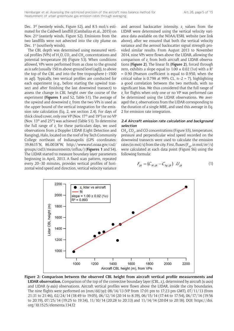
and aerosol backscatter intensity. zi values from the LIDAR were determined using the vertical velocity vari-ance data available on the NOAA/ESRL website (see link above), after we ensured that both the vertical velocity variance and the aerosol backscatter signal strength pro-vided similar results. From August 2013 to November 2014, nine VPs were flown above the LIDAR, allowing the comparison of zi from both aircraft and LIDAR observa-tions (Figure 2). The linear fit (Figure 2), forced through zero, exhibits a slope equal to 1.00 ± 0.02 (1σ) with a R2 = 0.90 (Pearson coefficient is equal to 0.950, when the critical value is 0.798 at 99% CL, n–2 = 7), highlighting a good correlation between the two methods, with no significant bias. We thus considered that the full range of zi for flights when only one or no VP was performed can be determined using the LIDAR observations. We aver-aged the zi observations from the LIDAR corresponding to the duration of a single MBE, and used this average in Eq. 2 for emission rate integration.

2.4 Aircraft emission rate calculation and background selectionCH4, CO2, and CO concentrations (Figure S5), temperature, pressure and perpendicular wind speed recorded on the downwind transects were used to calculate the emission rates (in mol/s) from the city. First, fluxes (Fijk, in mol/m2/s) were calculated at each data point (Figure S6) using the following formula:

, ,(   ) .ijk M ijk bg ijk ijkF C C U= − (1)

Figure 2: Comparison between the observed CBL height from aircraft vertical profile measurements and LIDAR observation. Comparison of the top of the convective boundary layer (CBL, zi), determined by aircraft (x-axis) and LIDAR (y-axis) observations. Aircraft vertical profiles were flown above the LIDAR, inside the city boundaries. The nine flights were performed on (mm/dd/yy): 08/14/13 (VP from 17:01 pm to 17:23 pm GMT), 07/11/13 (from 21:31 to 21:46), 02/24/14 (18:49 to 19:05), 06/12/14 (20:14 to 8:39), 06/15/14 (17:44 to 17:54), 06/17/14 (19:56 to 20:19), 07/25/14 (19:25 to 19:34), 11/10/14 (20:28 to 20:33) and 11/14/14 (20:04 to 20:18). DOI: https://doi.org/10.1525/elementa.134.f2

Heimburger et al: Assessing the optimized precision of the aircraft mass balance method for measurement of urban greenhouse gas emission rates through averaging

Art. 26, page 6 of 15

where CM,ijk is the concentration measured for a specific latitude (i), longitude (j) and height (k) and converted to mol/m3 using the ideal gas law (pressure and temperature are used to calculate molar density). Cbg,ijk represents background concentration (mol/m3, see below for more details), Uijk is the 10 s averaged perpendicular wind speed (m/s, Cambaliza et al., 2014). The term (CM,ijk – Cbg,ijk), also referred to as Eijk in the supplementary information, repre-sents the enhancement from the city. All the single-point horizontal fluxes are then projected onto a 2-D plane, and interpolated from the ground to the top of the bound-ary layer (zi, in m), to the edges of the downwind distance flown by the airplane using a multi-transect kriging approach, at 10 m (z-axis) × 100 m (x-axis) resolution (Matlab-based EasyKrig 3.0; Chu 2004; Mays et al., 2009; Cambaliza et al., 2014) (Figure S7), for integration (Eq. 2).

0

iz x

ijkx

ER F dx dz+

−=∫ ∫ (2)

Here, ER (mol/s) is the integrated emission rate for one MBE, –x and +x are the effective horizontal boundaries of the city, and dx and dz are the discrete horizontal and vertical distances (in m), over which the emission rate values are calculated, respectively. Whereas in Eq. 1 we calculate the flux through a vertical plane downwind of the city, in Eq. 2 we sum the flux in each interpolated pixel of that plane to calculate the total integrated emission rate from the city for a MBE. This produces a result which is consistent with what we observe, which is the total signal from all emission sources in the city. This distinguishes it from a surface flux, which can be calculated as a spatial average, e.g. as done by Mays et al. (2009). However, the surface fluxes are spatially highly heterogeneous (the power plant is a point source that represents roughly a third of the total, and mobile source emissions follow the major roads), and so calculated fluxes are not readily comparable between observations, while total emissions are much more so. And, the area used by Mays et al. (2009) represents an arbitrary choice of the definition of city boundaries. Thus we report only the total urban emissions for Indianapolis, in moles/s.

While entrainment/detrainment is possible, this has not been observed to date in our downwind vertical profiles. Typically, the boundary layer height does not increase by more than 15% and often less, during the course of the experiment. Because of this and the relatively short dis-tance of the downwind transects from city sources (~30 km), chosen to minimize time for full mixing to the top of the boundary layer, our method assumes that entrain-ment/detrainment effects are minimal. We should also note that since we designed these flights for the fully developed boundary layer afternoon period, our measure-ments reflect emission rates for that time of day, as well as the Fall season. We also calculated enhancements, and then fluxes, after interpolation of the data (kriging), i.e. at each gridded cell using interpolated GHG concentrations, pressure, temperature and perpendicular wind speed (Mays et al., 2009; Cambaliza et al., 2014, 2015), to assess any changes in emission rates due to the choice of the kriging approach. Results from the both methods are pre-sented in the “Results and Discussion”.

Concentrations from both edges of the downwind transects are considered to be equivalent to the inflow of background air on the upwind side of the city, as previ-ously defined by Mays et al. (2009) and Cambaliza et al. (2014, 2015) for aircraft measurements at Indianapolis. This approach was also used by Karion et al. (2015) for the Barnett Shale region. The location and distance of the transect edges were determined using a similar tech-nique proposed by Cambaliza et al. (2014), i.e. by i) pro-jecting the city boundaries onto the downwind transects using the observed mean wind direction, ii) observing the Gaussian shape of the CO2, CH4 and CO plumes recorded on these transects, and iii) defining the “edge” as the area of the transect where mixing ratios decrease to a constant concentration, and are likely not influenced by urban emissions. For all the flights, plumes from the city are well defined and concentrations decrease before reaching a constant concentration on both edges of the downwind transects. These edge concentrations are used for back-ground determination (Figures 3, S5).

In the interest of consistency, we defined backgrounds in two ways for all the flights. First, background concen-trations were defined as a single horizontally constant value, but varying with altitude (Cambaliza et al., 2014). This choice was motivated by the fact that significant background vertical gradients are observed for several flights, demonstrated on Dec. 3rd for CO2, CH4 and CO (Figure S5, see also vertical profiles on Figure S3), suggest-ing that altitude-dependent background concentrations, which might also vary with time and the growth of the CBL, should be determined for each individual downwind transect. Additionally, for some downwind transects, we observed that background concentrations on one edge can be significantly different from background concentra-tions observed on the opposite edge, suggesting a hori-zontal gradient in background concentration along the transect (see Nov. 25th, Figures 3 and S5). Therefore, back-grounds were also defined using a linear function passing through median concentrations of the two sets of edge concentrations for each downwind transect (Figures 3, S5). The slope and the y-intercept of the linear function are used to calculate background concentrations at each data point where a measurement was recorded (Cbg,ijk in Eq. 1). Consequences of background determination on emission rate results are discussed in the “Results and Discussion”.

For the Nov–Dec 2014 field campaign, we assumed constant emissions from CO2, CH4 and CO sources at Indianapolis such that each of the nine MBEs can be con-sidered as statistically repeated independent sampling of carbon emissions from the city. This is a reasonable assumption for CO and CO2 at a given climate condition for weekdays, and for CH4, given the diversity of sources in the city, either biogenic, or from the natural gas dis-tribution system (Lamb et al., 2016). Emission rates from the nine MBEs were then averaged and the standard error of the mean at 95% CL (also referred SEM95 hereafter) calculated as t s

n∗ , with t-student = 2.306, s is the sample

standard deviation from the nine MBEs, and n the number of experiments.

Heimburger et al: Assessing the optimized precision of the aircraft mass balance method for measurement of urban greenhouse gas emission rates through averaging

Art. 26, page 7 of 15

3. Results and discussion3.1 Method comparison To optimize our analysis method, data were processed using two different kriging approaches and background determinations. The background was defined i) as a single horizontal constant background concentration varying with altitude (BGavg) (Cambaliza et al., 2014) and ii) as a linear function to account for any horizontal gradient in background concentrations along the length of the down-wind transects (BGlinReg). We also interpolated i) concentra-tions, temperature, pressure and winds before calculating fluxes at each gridded cell (kriging_CTPU) (Mays et al., 2009; Cambaliza et al., 2014, 2015) or ii) individual point determinations of the calculated fluxes (kriging_Fijk).

Calculated average emission rates for CO2, CO, and CH4 are presented in Table 1, as a function of background selection and interpolation approach. When averaged, CO2, CO, and CH4 emission rates are statistically indistin-guishable using either BGavg or BGlinReg and kriging_Fijk or kriging_CTPU, as shown in Table 1. When BGavg is used with both the kriging_Fijk and kriging_CTPU approaches, CO2 SEM95 is equal to 45% and 39%, respectively, i.e. poorer than the 17% SEM95 (kriging_Fijk) and 25% SEM95 (kriging_CTPU) found when BGlinReg is applied. This result suggests that linear functions used to determine back-ground concentrations greatly reduce variability of CO2 emission rates calculated from replicate measurements. However, the SEM95 is similar for CO and CH4 regardless of the method of background determination. The use of kriging_CTPU or kriging_Fijk does not significantly change

the SEM95 of the method for CO2 and CO. For CH4, the SEM95 is improved by ~20% using kriging_CPTU instead of kriging_Fijk. However, the CH4 SEM95 remains large (41–60%, Table 1) compared to those for CO2 and CO for the same set of flights, suggesting that the CH4 emission rate variability is driven by factors other than the data analysis approach, and that for CH4, the assumption of constant emission rate is not robust. In the following, we use the kriging_Fijk approach with BGlinReg, since these two choices appear to yield the lowest SEM95 for the averaged CO2 and CO emission rates.

Cambaliza et al. (2014) demonstrated that the choice in background concentration determination is one of the most sensitive parameters impacting uncertainties and variability in the emission rate results. Of course, uncertainties in the calculated emission rates due to background depend significantly on the magnitude of the enhancement, i.e. that the uncertainties are larger for smaller enhancements. For the Nov.–Dec. 2014 flights, we observed that change in background determination can lead to significant change in the emission rate of a single MBE. When the method kriging_Fijk is applied, the average difference between emission rates of a MBE calculated using BGlinReg and using BGavg is 50% for CO2 (median = 9%), 32% for CH4 (median = 18%) and 13% for CO (median = 9%), and range from 1% – 198%, 7% – 150% and 1% – 35%, respectively (Figure 4, Table S2). The most significant differences are observed on Nov. 17th and 19th for CO2, and Dec. 3rd for CH4 (Figure 4, Table S2). However, given the presence of spatial gradients in

Figure 3: Downwind and upwind CO2 concentrations, and background as a function of distance. CO2 mole fraction in the downwind plume at different altitudes (blue, red and green full lines) and upwind the city (black full line), observed on November 25th, 2014 (wind direction = west, see Table S1). Dashed lines represent the background (as a linear regression) for each downwind transect. Higher background concentrations on the southern part of transects (positive distances) might be attributed to Eagle Valley power plant plume (see Figure 1). Vertical back lines represent the limits between background (BG, edges) and the city plume. DOI: https://doi.org/10.1525/elementa.134.f3

Heimburger et al: Assessing the optimized precision of the aircraft mass balance method for measurement of urban greenhouse gas emission rates through averaging

Art. 26, page 8 of 15

background, we regard it best to use the linear regression approach. These results do indicate that the CH4 emission rate determination is not more sensitive to background than is CO2, supporting our conclusions that the actual CH4 emission rates are variable day-to-day.

We also observed differences in calculated emis-sion rates for a single MBE depending on the choice of the kriging method (and for a same background determination) (Figure 4). For example, when BGlinReg is used, the averaged relative difference between the

Table 1: Comparison method: background selection and application of the kriging approach. Averaged CO2, CH4 and CO emission rates from the nine mass balance experiments (MBEs) i) when the emission rates were calculated by kriging the point fluxes (kriging_Fijk) and ii) when they were calculated and integrated after interpolation of concentrations, pressure, temperature and perpendicular wind speed (kriging_CTPU). For both interpolation methods, backgrounds were defined iii) as linear regression (BGlinReg) and iv) as averages (BGavg). Precision is the standard error of the mean at 95% CL. DOI: https://doi.org/10.1525/elementa.134.t1

Method BG CO2 emission rate

mean (mol/s)

Precision CO2

CH4 emission rate

mean (mol/s)

Precision CH4

CO emission rate

mean (mol/s)

Precision CO

kriging_Fijk BGlinReg 14600 ± 2500 17% 67 ± 40 60% 108 ± 17 16%

BGavg 10400 ± 4600 45% 81 ± 47 58% 98 ± 19 19%

kriging_CTPU BGlinReg 12400 ± 3200 25% 56 ± 23 42% 92 ± 13 14%

BGavg 11024 ± 4300 39% 65 ± 27 41% 91 ± 16 17%

Figure 4: Overview of emission rates results. Calculated emission rates for each flight experiment using the four approaches described in Section 3.2. DOI: https://doi.org/10.1525/elementa.134.f4

Heimburger et al: Assessing the optimized precision of the aircraft mass balance method for measurement of urban greenhouse gas emission rates through averaging

Art. 26, page 9 of 15

two kriging methods for a single flight is equal to 25% (median = 14%, range = 3% – 62%) for CO2, 25% (median = 21%, range = 6% – 58%) for CH4 and 24% (median = 17%, range = 3% – 66%) for CO (Table S2). However, we believe it is most logical to interpolate the individual fluxes, since this interpolation is conducted only for one data set (i.e. calculated point fluxes).

3.2 Improvement of CO2 fossil fuel and CO emission rate precision through averaging Table 2 summarizes emission rate results of the nine MBEs obtained from Eq. 1 and 2 (for kriging_Fijk and BGlinReg). Individual CO2, CO, and CH4 emission rates vary from 10,200 to 20,200 mol/s, 62 to 139 mol/s, and 16 to 189 mol/s, respectively (Figure 4). CO2 and CH4 emission rates are in the range of emission rates previously reported in Mays et al. (2009) and Cambaliza et al. (2014, 2015) for Indianapolis (from 2,500 to 49,000 mol/s for CO2 and 12 to 230 mol/s for CH4). When averaged, our measured emission rates are equal to 14,600 mol/s for CO2, 108 mol/s for CO and 67 mol/s for CH4. The average CO2 emis-sion rate for eight non-growing-season measurements in Mays et al. (2009) was 14,000 (±11,000; 1s) mol/s, for spring and winter of 2008. Our estimate via the Hestia emission model for the November 2014 CO2 daytime (1200–1600) fossil fuel emission rate for Marion County, which corresponds to the way the downwind transects cut across the city, is 15,100 mol/s, which is indistinguishable from our average. Lauvaux et al. (2016), using an inverse modeling approach, have reported a value of 22,300 mol/s for the non-growing season for a larger 9-county region around Marion County, which they compare to the corresponding 9-county Hestia value of 18,300 mol/s. So, if the inverse model result scales with the relative Hestia

values, the corresponding Lauvaux et al. inverse model value for Marion County would be 18,400 mol/s. For CH4, our average value, from 43 flights from 2008–2016, is 95 (±21) mol/s at the 95% CL. Although there are few city-wide estimates of GHG emissions, O’Shea at al., (2014) use aircraft-based measurements and the mass balance approach to determine the CO2, CH4 and CO emission rates from London, UK. They measured emission rates of 36,000 ± 3300 mol/s, 240 ± 16 mol/s and 220 ± 8 mol/s for CO2, CH4 and CO, respectively. These emission rates are considerably greater than those measured for Indianapo-lis, which is likely due, in part, by the larger population in London (appx 8.6 million) and older infrastructure.

Estimation of the uncertainty for a single MBE (∆ER, see Text S1 in supplementary information, Table S3) was calcu-lated by propagating i) the measurement uncertainties of each term involved in Eq. 1, (i.e. uncertainties in pressure and temperature, which were used to convert into units of mol/m3, uncertainties of the calibration and from the linear fit for background determination and in the wind speed) and ii) the uncertainty of the CBL height due to growth during the experiment. Our uncertainty estimate represents a lower limit of the uncertainty associated with a single MBE, since all the factors known to influ-ence emission rate results, such as entrainment from the free troposphere and interpolation of data points using the kriging approach (Cambaliza et al., 2014), were not accounted for. Relative uncertainties (RSD% = ∆ER/ER) calculated from the uncertainty estimate of single MBEs vary between 23% and 91% (average = 44%) for CO2, 24% and 81% (average = 42%) for CO, and 25% and 153% (average = 67%) for CH4 (Table 1). When emission rates are averaged over the nine MBEs, the SEM95 (represent-ing the expected precision for replication of a nine-point

Table 2: CO2, CH4 and CO emission rates from single mass balance experiments and average. CO2, CH4 and CO emission rates (mol/s) for single mass balance experiments (MBEs), their respective absolute uncertainties ( propagation of uncertainties, results at 95% CL, see supplementary information) and relative precision. The averaged emission rates are reported with the standard error of the mean at 95% CL. The kriging approach was directly applied on fluxes (kriging_Fijk). Background concentrations were calculated from linear functions. DOI: https://doi.org/10.1525/elementa.134.t2

Flight dates in 2014 (mm/dd)

CO2 emission rate (mol/s)

Precision CH4 emission rate (mol/s)

Precision CO emission rate (mol/s)

PrecisionCO2 CH4 CO

11/13 13600 ± 3000 23% 101 ± 30 30% 111 ± 26 24%

11/14 11700 ± 10700 91% 54 ± 44 82% 119 ± 68 58%

11/17 19500 ± 17000 88% 74 ± 110 153% 139 ± 110 81%

11/19 20200 ± 6240 32% 189 ± 100 53% 96 ± 57 59%

11/20 13800 ± 3700 28% 22 ± 13 56% 111 ± 41 37%

11/21 14000 ± 3900 29% 50 ± 14 29% 101 ± 29 29%

11/25 14600 ± 3500 25% 56 ± 14 26% 129 ± 34 26%

12/01 14000 ± 3400 25% 45 ± 11 25% 100 ± 31 31%

12/03 10200 ± 5400 53% 16 ± 24 150% 62 ± 21 33%

Average14600 ± 2500 17% 67 ± 40 60% 108 ± 17 16%

Nov–Dec

Heimburger et al: Assessing the optimized precision of the aircraft mass balance method for measurement of urban greenhouse gas emission rates through averaging

Art. 26, page 10 of 15

mean) is equal to 17% for CO2, 16% for CO, and 60% for CH4. Although the CH4 variability is large, the precision of the mean for CO2 and CO, when calculated from several MBEs performed in a short period of time (so that the emissions can be assumed to be constant), represents a significant improvement compared to the measurement uncertainty estimated for a single MBE measurement (and as shown by Cambaliza et al. (2014) to be 40–50%). This averaging approach represents a considerable improve-ment compared to the commonly reported uncertainties of GHG emission measurements from urban environ-ments (~50% up to 100%; Trainer et al., 1995; Gurney et al., 2009; Mays et al., 2009; NRC, 2010; Turnbull et al., 2011; Cambaliza et al., 2014, 2015). Since the results for CH4 are very different, for the same set of flight data, it seems clear that the emission rate variability is substan-tially different for CH4.

The proposed averaging method has several potential limitations. All of the MBEs in this study were performed during the late fall when the total CO2 enhancement from Indianapolis can be attributed to urban fossil fuel-related sources and biogenic CO2 can be considered negligible (Turnbull et al., 2015). Also during the late fall, the mobile sector is the dominant source of CO emissions (Turnbull et al., 2015). The interpretation of the SEM95 is also based on the assumption that fossil fuel-related CO2, CO, and CH4 emissions from Indianapolis are constant during the three-week sampling period. In reality, some daily variability in urban emissions occurs (e.g. due to vari-ability in ambient temperature and subsequent heating and electric power requirements), which may contribute to a larger (poorer) apparent estimated precision. Thus the SEM95 results obtained here are upper limits to the method precision for the period of year considered here, and it is likely that the true method precision is better than reflected in the SEM95 for CO2 and CO.

3.3 Variability of CH4 emissionsAs discussed above, CH4 emissions for Indianapolis are considerably more variable day-to-day than are those of CO2 and CO. The averaged CH4 emission rate (67 ± 40 mol/s) found for late fall 2014 is close to the emission rate calculated from a bottom-up inventory (57 mol/s, Lamb et al., 2016) built with measurements of selected sources in the city, including natural gas distribution facilities, landfills and waste water treatment facilities. The range of the CH4 emission rate for the late fall overlaps with but is significantly lower than the range reported for spring-summer 2011 at Indianapolis (135 ± 58 mol/s, averaged from five airborne MBEs; Cambaliza et al., 2015), implying considerable variability for methane.

As shown by Cambaliza et al. (2015), the large enhancement of CH4 signal from the south side of Indianapolis is attributed to the Southside landfill (SSLF, Figure 1), which represents a significant portion of the city-wide CH4 emissions. We used wind direction data recorded by the BAT probe and the Hybrid Single Particle Lagrangian Integrated Trajectory Model (HYSPLIT, Draxler and Rolph, 2012) to confirm that the large CH4 enhance-ments observed in fall 2014 (Figure S5b) can also be

attributed to the SSLF emissions. Cambaliza et al. (2015) determined that the SSLF represented, on average, 33% of the total CH4 emissions from Indianapolis. Lamb et al. (2016) reported an average CH4 emission rate of 31 mol/s for the SSLF, using ground-based mobile sampling for inverse plume modeling, and 30 mol/s is obtained from the EPA’s GHG Reporting Program. If we assume that the CH4 average we obtained (67 mol/s) for the city-wide total is representative, the Lamb et al. (2016) value for the SSLF represents 46% of the city-wide total. Variability of CH4 emissions from landfills is partially dependent on the local climate, which can influence the seasonal oxidation of landfill covers (Xu et al., 2014; Spokas et al., 2015). To better understand the variability of the SSLF emissions, we considered several factors known to influence landfill emissions, such as change in barometric pressure over time, air temperature and precipitation (Xu et al., 2014; Spokas et al., 2015). However, no particular correlations were found between aircraft-determined CH4 emission rates (the part attributed to the landfill) and average atmos-pheric temperature recorded at Indianapolis International airport during the experiments (data downloaded from http://www.ncdc.noaa.gov/qclcd/QCLCD, accessed on 10/05/2015), as well as with relative humidity and baro-metric pressure. Lamb et al. (2016) report that the uncer-tainty in their determination of the SSLF emission rate is ±30%, or 9 mol/s. In contrast, the SEM95 for the city-wide total we determined is 40 mol/s (60%), i.e. much larger than the SSLF uncertainty, and larger than the average SSLF emission rate reported by Lamb et al. (2016). The total CH4 variability must, then, derive from CH4 sources other than the landfill and must be large enough to explain the high variability of the city-wide CH4 emission rate (SEM95 of 60%). Using the ratio of propane-to-methane ((C3H8)/CH4) concentrations from aircraft flask samples and the slope of the C3H8 vs. CH4 regression, Cambaliza et al (2015) demonstrated that the non-landfill-related CH4 emissions from Indianapolis represent ~67% of the total CH4 emis-sions and could be attributed to the natural gas distribu-tion system. Lamb et al. (2016) estimated a contribution of natural gas sources of 43% from ethane/methane observation coupled with inverse modeling. The authors also found that emissions from natural gas systems can vary by three orders of magnitude, depending on the type of structures in the natural gas system (i.e., pipeline, transmission and storage station, etc.). Emissions from the natural gas system at Indianapolis are potentially due to random small sources (Lamb et al., 2016) and can be highly spatially and temporally variable, which likely explains the variability of CH4 emission rates we observed in Nov.–Dec. 2014. However, to explain our observed vari-ability, we would need to turn to large GHG contributors, among which are the natural gas sources.

4. ConclusionsFrom nine mass balance experiments performed in Indi-anapolis in Nov.–Dec. 2014, we quantified averaged CO2, CO, and CH4 emission rates (14,600, 108 and 67 mol/s, respectively). The SEM95 results were equal to 17% for CO2

and 16% for CO (at the 95% CL), i.e. much lower than for

Heimburger et al: Assessing the optimized precision of the aircraft mass balance method for measurement of urban greenhouse gas emission rates through averaging

Art. 26, page 11 of 15

the single-flight precision (~40%) found for Indianapolis (Cambaliza et al., 2014), and for the estimated single-flight uncertainties for the results reported here. We applied averaging to improve estimation of CO2 and CO urban emission rates during the late fall, when CO2 and CO emis-sions are primarily of anthropogenic origin. During the summer, poorer apparent precision would be expected due to the greater CO2 and CO emissions variability from biogenic emission contributions. A field campaign similar to the one presented in this study (multiple MBEs flown in a short period of time, to allow for an assumption of constant emission rates over the time period) should be performed during the spring and summer seasons to eval-uate the averaging method when biogenic CO2 and CO emissions are not negligible. While the precision obtained in this mass balance experiment is approaching GHG reduction target values, we expect averaged emission rate precisions to be further improved with increasing num-bers of airborne MBEs performed over a short period of time. Precisions might also be further improved by either the use of multiple aircraft flying simultaneously, or one aircraft flying at the top of the boundary layer and employing a downward-looking Differential Absorption LIDAR (Dobler et al., 2013; Abshire et al., 2014). Thus the target precision is technically attainable, the main limita-tion being the cost of the experiment.

Previous aircraft and surface-based measurements have suggested that most of the remaining CH4 (~2/3 of the city-wide emissions) likely derives from the city’s natural gas distribution system (Cambaliza et al., 2015; Lamb et al., 2016). Since the Southside Landfill is a minor com-ponent of the total, and the remainder is believed to be derived from the natural gas network, it appears that the variability in our observations of the city-wide total may be attributed to variability in the nature and magnitude of individual leaks in that system. Surface-based meas-urements of methane, ethane, and d13C-CH4 may allow us to differentiate between CH4 sources, complementing the aircraft-based total emission rate measurement. For this city, evaluation of emission mitigation progress for methane may be difficult because of the large day-to-day variability in the source strength.

Data Accessibility Statement Data presented in this paper are available on the INFLUX webpage (http://sites.psu.edu/influx/) and upon request from the corresponding author.

Supplemental FilesThe supplemental files for this article can be found as follows:

• Text S1. Uncertainties for a single MBE. DOI: https://doi.org/10.1525/elementa.134.s1

• Figure S1. CRDS calibration. DOI: https://doi.org/10.1525/elementa.134.s2

• Figure S2. Flight paths of the aircraft experiments. DOI: https://doi.org/10.1525/elementa.134.s3

• Figure S3. Aircraft vertical profiles and esti-mated boundary layer height. DOI: https://doi.org/10.1525/elementa.134.s4

• Figure S4. LIDAR observations. DOI: https://doi.org/10.1525/elementa.134.s5

• Figure S5. Downwind CO2, CH4 and CO concentra-tions as a function of distance. DOI: https://doi.org/10.1525/elementa.134.s6

• Figure S6. Downwind CO2, CH4 and CO fluxes, observations. DOI: https://doi.org/10.1525/elemen-ta.134.s7

• Figure S7. Downwind CO2, CH4 and CO fluxes after data interpolation (kriging). DOI: https://doi.org/10.1525/elementa.134.s8

• Table S1. Meteorological conditions during the field campaign. DOI: https://doi.org/10.1525/elemen-ta.134.s9

• Table S2. Emission rates depending on background determination and the kriging method. DOI: https://doi.org/10.1525/elementa.134.s10

• Table S3. Uncertainties of individual MBEs. DOI: https://doi.org/10.1525/elementa.134.s11

AcknowledgementsWe would like to acknowledge the Purdue University Jonathan Amy Facility for Chemistry Instrumentation (JAFCI) for technical support on the project. We also thank pilots R. M. Grundman and J. N. Poppe, who performed the MBEs with us.

Funding informationThis work is part of the Indianapolis Flux Experiment (INFLUX) project, funded by the National Institute of Standards and Technology (NIST), for which we are grateful.

Competing interestsThe authors have no competing interests to declare.

Author contibutions• Project conception and design: AMFH, PBS, BS, MOLC• Data Acquisition: AMFH, PBS• Analysis and interpretation of data: AMFH, RMH,

PBS, CS, JT, OES, A-EMK, TNL• Drafting and/or revising the article: AMFH, RMH,

PBS, JT, MOLC, OES, A-EMK, TNL, KJD, TL, AK, CS, WAB, RMH, KRG, JW

• Final approval of the version to be published: AMFH, RMH, PBS

ReferencesAbshire, JB, Ramanathan, A, Risis, H, Mao, J, Allan, GR,

et al. 2014 Airborne Measurements of CO2 column concentration and range using a pulsed direct-detection IPDA Lidar. Remote Sens 6: 443–469. DOI: https://doi.org/10.3390/rs6010443

Bergamaschi, P, Corazza, M, Karstens, U, Athanassiadou, M, Thompson, RL, et al. 2015 Top-down estimates of European CH4 and N2O emissions based on four different inverse models. Atmos Chem Phys 15: 715–736. DOI: https://doi.org/10.5194/acp-15-715-2015

Bousquet, P, Ciais, C, Miller, JB, Dlugokencky, EJ, Hauglustaine, DA, et al. 2006 Contribution of anthropogénique and natural sources to atmospheric

Heimburger et al: Assessing the optimized precision of the aircraft mass balance method for measurement of urban greenhouse gas emission rates through averaging

Art. 26, page 12 of 15

methane variability. Nature 443: 439–443. DOI: https://doi.org/10.1038/nature05132

Cambaliza, MOL, Bogner, JE, Green, RB, Shepson, PB, Harvey, TA, et al. 2017 Field measurements and modeling to resolve m2 to km2 CH4 emissions for a complex urban source: An Indiana landfill study, Elem Sci Anth., in press for INFLUX special feature.

Cambaliza, MOL, Shepson, PB, Bogner, J, Caulton, DR, Stirm, B, et al. 2015 Quantification and source appor-tionment of the methane emission flux from the city of Indianapolis. Elem Sci Anth. 3: 000037. DOI: https://doi.org/10.12952/journal.elementa.000037

Cambaliza, MOL, Shepson, PB, Caulton, DR, Stirm, B, Samarov, D, et al. 2014 Assessment of uncertain-ties of an aircraft-based mass balance approach for quantifying urban greenhouse gas emissions. Atmos Chem Phys 14: 9029–9050. DOI: https://doi.org/10.5194/acp-14-9029-2014

Carras, JN, Cope, M, Lilley, W and Williams, DJ 2002 Measurement and modeling of pollutant emissions from Hong Kong. Environ Modeling & Software 17: 87–94. DOI: https://doi.org/10.1016/S1364-8152(01)00055-X

China’s INDC Enhanced actions on climate change: China’s intended nationally determined contribu-tions. June 2015. Available at http://www4.unfccc.int/submissions/INDC/Published%20Documents/China/1/China’s%20INDC%20-%20on%2030%20June%202015.pdf. Accessed December 2015.

Chu, D 2004 The GLOBEC kriging software package – EasyKrig 3.0; The Woods Hole Oceanographic Institution. Available at http://globec.whoi.edu/software/kriging/easy_krig/easy_krig.html. Accessed May 2015.

Crawford, TL and Dobosy, RJ 1992 A sensitive fast-response probe to measure turbulence and heat flux from any airplane. Boundary Layer Meteor 59(3): 257–278. DOI: https://doi.org/10.1007/BF00119816

Crosson, ER 2008 A cavity ring-down analyzer for measur-ing atmospheric levels of methane, carbon dioxide, and water vapor. Appl Phys B-Lasers O 92: 403–408. DOI: https://doi.org/10.1007/s00340-008-3135-y

Dobler, JT, Harisson, FW, Browell, EV, Lin, B, McGregor, D, et al. 2013 Atmospheric CO2 column measurements with an airborne intensity-modu-lated continuous wave 1.57 µm fiber laser lidar. Applied Optics 52(12): 2,874–2,892. DOI: https://doi.org/10.1364/AO.52.002874

Draxler, RR and Rolph, GD 2012 HYSPLIT (Hybrid Single-Particle Lagrangian Integrated Trajectory) Model access via NOAA ARL READY website NOAA Air Resources Laboratory, Silver Srping, MD. Available at http://ready.arl.noaa.gov/HYSLIPT.php?.

European commission 2014 Progress towards achiev-ing the Kyoto and EU 2020 objectives. Available at http://ec.europa.eu/transparency/regdoc/rep/1/2014/EN/1-2014-689-EN-F1-1.Pdf.

Forster, P, Ramaswamy, V, Artaxo, P, Berntsen, T, Betts, R, et al. 2007 Changes in Atmospheric

Constituents and in Radiative Forcing. In: Climate Change 2007: The Physical Science Basis. Contribution of Working Group I to the Fourth Assessment Report of the Intergovernmental Panel on ClimateChange. Cambridge University Press, Cambridge, United Kingdom and New York, NY, USA. Solomon, S, Qin, D, Manning, M, Chen, M, Marquis, M, Averyt, KB, Tignor, M and Miller, HL, (eds.).

Garman, KE, Hill, KA, Wyss, P, Carlsen, M, Zimmerman, JR, et al. 2006 An airbone and wind tunnel evaluation of a wind turbulence measure-ment system for aircraft-based flux measurement. J Atmos Ocean Tech 23: 1696–1708. DOI: https://doi.org/10.1175/JTECH1940.1

Garman, KE, Wyss, P, Carlsen, M, Zimmerman, JR, Stirm, BH, et al. 2008 The contribution of vari-ability of lift-induced upwash to the uncertainty in vertical winds determined from an aircraft platform. Boundary Layer Meteor 126: 461–476. DOI: https://doi.org/10.1007/s10661-013-3517-4

Gioli, B, Carfora, MF, Magliulo, V, Metallo, MC, Poli, AA, et al. 2014 Aircraft mass budgeting to measure CO2 emissions from Rome, Italy. Environ Monit Assess 186: 2053–2066. DOI: https://doi.org/10.1007/s10661-013-3517-4

Gurney, KR, Mendoza, DL, Zhou, Y, Fischer, ML, Miller, CC, et al. 2009 High resolution fossil fuel combustion CO2 emission fluxes for the United States. Environ Sci Technol 43: 5535–5541. DOI: https://doi.org/10.1021/es900806c

Gurney, KR, Razlivanov, I, Song, Y, Zhou, Y, Benes, B, et al. 2012 Quantification of fossil fuel CO2 emis-sions at the building/street level scale for a large US city. Environ Sci Technol 46: 12194–12202. DOI: https://doi.org/10.1021/es3011282

Hutyra, LR, Duren, R, Gurney, KR, Grimm, N, Kort, EA, et al. 2014 Urbanization and the carbon cycle: Current capabilities and research outlook from the natural sciences perspective. Earth’s future 2: 473–495 DOI: https://doi.org/10.1002/2014EF000255

IEA (International Energy Agency) 2008 World energy outlook. Available at http://www.worldenergy-outlook.org/media/weowebsite/2008-1994/weo2008.pdf.

IPCC (Intergovernmental Panel on Climate Change) 2014 Climate Change 2014: Mitigation of Climate Change, Contribution of Working Group III to the Fifth Assessment Report of the Intergovernmental Panel on Climate Change, Chapter 12, p. 935 [ Edenhofer, O, Pichs-Madruga, RR, Sokona, Y, Farahani, E, Kadner, S, Seyboth, K, Adler, A, Baum, I, Brunner, S, Eickemeier, P, Kriemann, B, Savolainen, J, Schlömer, S, von Stechow, C, Zwickel, T and Minx, JC, (eds.)]. Available at http://mitigation2014.org/report/publication/.

Kalthoff, N, Corsmeier, U, Schmidt, K, Kottmeier, C, Fiedler, F, et al. 2002 Emissions of the city of Augs-burg determined using the mass balance method. Atmos Environ 36(Supplement 1): 19–S31. DOI: https://doi.org/10.1016/S1352-2310(02)00215-7

Heimburger et al: Assessing the optimized precision of the aircraft mass balance method for measurement of urban greenhouse gas emission rates through averaging

Art. 26, page 13 of 15

Karion, A, Sweeney, C, Kort, EA, Shepson, PB, Brewer, A, et al. 2015 Aircraft-based estimate of total methane emissions from the Barnett shale region. Environ Sci Technol 49: 8124–8131. DOI: https://doi.org/10.1021/acs.est.5b00217

Karion, A, Sweeney, C, Pétron, G, Frost, G, Hardesty, MH, et al. 2013b Methane emissions estimate from air-borne measurements over the western United Sates natural gas field, Geophys Res Lett 40: 4393–4397. DOI: https://doi.org/10.1002/grl.50811

Karion, A, Sweeney, C, Wolter, S, Newberger, T, Chen, H, et al. 2013a Long-term greenhouse gas measure-ments from aircraft. Atmos Meas Tech 6: 511–526. DOI: https://doi.org/10.5194/amt-6-511-2013

Kirschke, S, Bousquet, P, Ciais, P, Saunois, M, Canadell, JG, et al. 2013 Three decades of global methane sources and sinks. Nature Geosci 6: 813–823. DOI: https://doi.org/10.1038/ngeo1955

Lamb, BK, Prasad, K, Cambaliza, MO, Ferrara, T, Lauvaux, T, et al. 2016 n.d. Direct and indirect measurements and modeling of methane emis-sions in Indianapolis, IN., Environ. Sci. Technol., submitted. DOI: https://doi.org/10.1021/acs.est.6b01198

Lauvaux, TN, Miles, A, Deng, S, Richardson, M, Cambaliza, O, Davis, K, Brian Gaudet, K, Gurney, J, Huang, D, o’Keefe, Y, Song, A, Karion, T, Oda, R, Patarasuk, I, Razlivanov, D, Sarmiento, PB, Shepson, C, Sweeney, J and Turnbull Wu, K 2016 High-resolution atmospheric inversion of urban CO2 emissions during the dormant season of the Indianapolis Flux Experiment (INFLUX), J. Geophys. Res. Atmos., 121, DOI: https://doi.org/10.1002/2015JD024473

Le Quéré, C, Moriarty, R, Andrew, RM, Peters, GP, Ciais, P, et al. 2014 Global carbon budget 2014. Earth Syst Sci Data Duscuss 7: 521–610. DOI: https://doi.org/10.5194/essdd-7-521-2014

Lind, JA and Kok, GL 1999 Emission strengths for pri-mary pollutants as estimated from an aircraft study of Hong Kong air quality. Atmos Environ 33: 825–831. DOI: https://doi.org/10.1016/S1352-2310(98)00141-1

Marland, G 2008 Uncertainties in accounting for CO2

from fossil fuels. J Ind Ecol 12: 136–139. DOI: https://doi.org/10.1111/j.1530-9290.2008.00014.x

Marland, G 2012 China’s uncertain CO2 emissions. Nature Clim Change 2: 645 – 646. DOI: https://doi.org/10.1038/nclimate1670

Mays, KL, Shepson, PB, Stirm, BH, Karion, A, Sweeney, C, et al. 2009 Aircraft-based measure-ments of the carbon footprint of Indianapolis. Environ Sci Technol 43: 7816–7823. DOI: https://doi.org/10.1021/es901326b

McKain, K, Down, A, Raciti, SM, Budney, J, Hutyra, LR, et al. 2015 Methane emissions from natural gas infrastructure and use in the urban region of Boston, Massachusetts. Proc Nati Acad Sci USA 112(7): 1,941–1,956. DOI: https://doi.org/10.1073/pnas.1416261112

Miles, NK, Richardson, SJ, Lauvaux, T, Davis, KJ, Deng, AJ, et al. 2015 May 20. Detection and quanti-fication of atmospheric boundary layer greenhouse gas dry mole fraction enhancements from urban emission: results from INFLUX. NOAA GMD annual meeting; Boulder, CO.

Myhre, G, Shindell, D, Bréon, F-M, Collins, W, Fuglestvedt, J, et al. 2013 Anthropogenic and Natural Radiative Forcing. In Climate Change 2013: The Physical Science Basis. Contribution of Working Group I to the Fifth Assessment Report of the I ntergovernmental Panel on Climate Change. Cambridge University Press, Cambridge, UK and New York, NY, USA. pp: 659–740. Stocker, TF, Qin, D, Plattner, G-K, Tignor, M, Allen, SK, Boschung, J, Nauels, A, Xia, Y, Bex, V and Midgley, PM, (eds.).

Nisbet, E and Weiss, R 2010 Top-down versus Bottom-up. Science 328(5983): 1241–1243. DOI: https://doi.org/10.1126/science.1189936

NRC 2010 (Committee on Methods for Estimating Green-house Gas Emisisons), Verifying Greenhouse Gas Emissions: Methods to Support International Climate Agreements, report n° 9780309152112, The National Academies Press, Washington DC.

Olivier, JGJ, Bouwman, AF, van der Maas, CWM, Berdowski, JJM, Veldt, C, et al. 1996 Descrip-tion of Edgar Version 2.0: A set of global emission inventories of greenhouse gases and ozone-depleting substances for all anthropogenic and most natural sources on a per country basis and on 1° × 1° grid. RIVM report nr. 771060 002/TNO-MEP report nr. R96/119. National Institute of Public Health and the Environment, Bilthoven, The Netherlands.

O’Shea, SJ, Allen, G, Fleming, ZL, et al. 2014b Area fluxes of carbon dioxide, methane, and carbon monoxide derived from airborne measurements around Greater London: A case study during summer 2012. J Geophys Res-Atmos 119: 4940–4952. DOI: https://doi.org/10.1002/2013JD021269

O’Shea, SJ, Allen, G, Gallagher, MW, et al. 2014a Methane and carbon dioxide fluxes and their regional scalability for the European Arctic wetlands during the MAMM project in summer 2012, Atmos. Chem. Phys 14: 13159–13174. DOI: https://doi.org/10.5194/acp-14-13159-2014

Parrish, DD, Trainer, M, Holloway, JS, Yee, J, Warshawsky, S, et al. 1993 Relationships between ozone and carbon monoxide at surface sites in the North Atlantic region, J Geophys Res 103: 13357–13376. DOI: https://doi.org/10.1029/98JD00376

Peylin, P, Houweling, S, Krol, MC, Karstens, U, Rödenbeck, C, et al. 2011 Importance of fossil fuel emission uncertainties over Europe for CO2 mod-eling: model intercomparison, Atmos Chem Phys 11: 6607–6622. DOI: https://doi.org/10.5194/acp-11-6607-2011

President’s Climate Action Plan 2013 Available at http://www.whitehouse.gov/sites/default/files/image/president27sclimateactionplan.pdf.

Heimburger et al: Assessing the optimized precision of the aircraft mass balance method for measurement of urban greenhouse gas emission rates through averaging

Art. 26, page 14 of 15

President Obama’s Climate Action Plan 2014a Progress Report, Cutting carbon pollution, protecting American communities, and leading internationally. Available at http://www.whitehouse.gov/sites/default/files/docs/cap_progress_report_update_062514_final.pdf.

President’s Climate Action Plan 2014b Strategy to reduce methane emissions. Available at http://www.whitehouse.gov/sites/default/files/strategy_to_reduce_methane_emissions_2014-03-28_final.pdf.

Rosenzweig, C, Solecki, W, Hammer, SA and Mehrotra, S 2010 Cities lead the way in climate-change action. Nature 467: 909–911. DOI: https://doi.org/10.1038/467909a

Schakenbach, J, Vollaro, R and Forte, R 2006 Fun-damentals of Successful Monitoring, Reporting, and Verification under a Cap-and-Trade Program. J of the Air & Waste Management Association 56: 1576–1583. DOI: https://doi.org/10.1080/10473289.2006.10464565

Seto, KC, Güneralp, B and Hutyra, LR 2012 Global fore-cast of urban expansion to 2030 and direct impacts on biodiversity and carbon pools. Proc Natl Acad Sci USA 109: 16083–16088. DOI: https://doi.org/10.1073/pnas.1117622109

Spokas, K, Bogner, J, Corcoran, M and Walker, S 2015 From California dreaming to California data: challenging historic models for landfill CH4 emissions. Elementa 3: 000051. DOI: https://doi.org/10.12952/journal.elemena.000051

Sweeney, C, Karion, A, Wolter, S, Newberger, T, Guenther, D, et al. 2015 Seasonal climatology of CO2 across North America from aircraft measurements in the NOAA/ESRL Global Greenhouse Gas Reference Network. J Geophys Res-Atmos 120: 5155–5190. DOI: https://doi.org/10.1002/2014JD022591

Trainer, M, Ridley, BA, Burh, MP, Kok, G, Walega, J, et al. 1995 Regional ozone and urban plumes in the southeastern United States: Birmingham, a case study. J Geophys Res 100: 18,823–18,834. DOI: https://doi.org/10.1029/95JD01641

Turnbull, JC, Guenther, D, Karion, A, Sweeney, C, Anderson, E, et al. 2012 An integrated flask sample collection system for greenhouse gas measurements. Atmos Meas Tech 5: 2321–2327. DOI: https://doi.org/10.5194/amt-5-2321-2012

Turnbull, JC, Karion, A, Fisher, ML, Faloona, I, Guilderson, T, et al. 2011 Assessment of fossil

fuel carbon dioxide and other anthropogenic trace gas emissions from airborne measurements over Sacramento, California in spring 2009. Atmos Chem Phys 11: 705–721. DOI: https://doi.org/10.5194/acp-11-705-2011

Turnbull, JC, Sweeney, C, Karion, A, Newberger, T, Lehman, SJ, et al. 2015 Toward quantification and source sector identification of fossil fuel CO2 emis-sions from an urban area: results from the INFLUX experiment. J Geophys Res Atmos 120: 292–312. DOI: https://doi.org/10.1002/2014JD022555

United Nations Framework Convention on Climate Change (UNFCCC) 2010 Report of the Confer-ence of the Partie on its fifteenth session, held in Copenhagen form 7 to 10 December 2009. FCCC/CP/2009/Add.1. Available at http://unfccc.int/resource/docs/2009/cop15/eng/11a01.pdf. Appendix I available at http://unfccc.int/meetings/copenhagen_dec_2009/items/5264.php.

United Nations Framework Convention on Climate Change (UNFCCC) 2015 Adoption of the Paris Agreement. FCCC/CP/2015/L.9/Rev.1. Available at https://unfccc.int/resource/docs/2015/cop21/eng/l09r01.pdf.

Vine, E and Sathaye, J 1999 The monitoring, evaluation, reporting and verification of climate change pro-jects. Mitig Adapt Strateg Glob Change 4(1): 43–60. DOI: https://doi.org/10.1023/A:1009651316596

Wennberg, PO, Mui, W, Wunch, D, Kort, EA, Blake, DR, et al. 2012 On the sources of methane to the Los Angeles atmosphere. Environ Sci Technol 46(17): 9,282–9,289. DOI: https://doi.org/10.1021/es301138y

White, WH, Anderson, JA, Blumenthal, DL, Husar, RB, Gillani, NV, et al. 1976 Formation and Transport of Secondary Air Pollutants: Ozone and Aerosols in the St. Louis Urban Plume. Science 194(4261): 187–189. DOI: https://doi.org/10.1126/science.959846

Wunch, D, Wennberg, PO, Toon, GC, Keppel-Aleks, G and Yavin, YG 2009 Emissions of greenhouse gases from a North American megacity. Geo-phys Res Lett 36(L15): 810. DOI: https://doi.org/10.1029/2009GL039825

Xu, L, Lin, X, Amen, J, Welding, K and McDermitt, D 2014 Impact of changes in barometric pres-sure on landfill methane emission. Global Biogeochem Cy 28: 679–695. DOI: https://doi.org/10.1002/2013GB004571

Heimburger et al: Assessing the optimized precision of the aircraft mass balance method for measurement of urban greenhouse gas emission rates through averaging

Art. 26, page 15 of 15

How to cite this article: Heimburger, AMF, Harvey, RM, Shepson, PB, Stirm, BH, Gore, C, Turnbull, J, Cambaliza, MOL, Salmon, OE, Kerlo, A-EM, Lavoie, TN, Davis, KJ, Lauvaux, T, Karion, A, Sweeney, C, Brewer, WA, Hardesty, RM and Gurney, KR 2017 Assessing the optimized precision of the aircraft mass balance method for measurement of urban greenhouse gas emission rates through averaging. Elem Sci Anth, 5: 26, DOI: https://doi.org/10.1525/elementa.134

Domain Editor-in-Chief: Detlev Helmig, University of Colorado Boulder, US

Guest Editor: Armin Wisthaler, University of Oslo, NO

Knowledge Domain: Atmospheric Science

Part of an Elementa Special Feature: Quantification of urban greenhouse gas emissions: The Indianapolis Flux experiment

Submitted: 24 October 2016 Accepted: 19 April 2017 Published: 07 June 2017

Copyright: © 2017 The Author(s). This is an open-access article distributed under the terms of the Creative Commons Attribution 4.0 International License (CC-BY 4.0), which permits unrestricted use, distribution, and reproduction in any medium, provided the original author and source are credited. See http://creativecommons.org/licenses/by/4.0/. OPEN ACCESS Elem Sci Anth is a peer-reviewed open access

journal published by University of California Press.