ASSESSING THE IMPACTS OF STATE-SUPPORTED RAIL …

1

ASSESSING THE IMPACTS OF STATE-SUPPORTED RAIL SERVICES ON 1

LOCAL POPULATION AND EMPLOYMENT: A CALIFORNIA CASE STUDY 2

3

Ahmadreza Talebiana,1, Bo Zoua, Mark Hansenb 4

5

a Department of Civil and Materials Engineering, University of Illinois at Chicago, United States 6

b Department of Civil and Environmental Engineering, University of California at Berkeley, United States 7

8

Abstract: The State of California has been financially supporting Amtrak intercity passenger rail 9 services since 1976. This paper studies the impacts of this support on local population and 10 employment at both county and city levels. We use datasets which include geographic, transport, and 11 socioeconomic characteristics of California counties and cities from 1950 to 2010. Propensity score, 12 one-to-one matching models are employed to draw units from the control group, which are 13 counties/cities that do not have a state-supported Amtrak station, to match with units from the 14 treatment group, which are counties/cities that do. Using regression analysis, we find that state-15 support Amtrak stations have significant effect on local population in the long term, and the effect 16 increases with time. However, the effect on civilian employment is almost non-existent. This suggests 17 that state-supported Amtrak services can provide quality rail mobility and accessibility, which attract 18 people to live in a rail-accessible region. However, the economic influence seems limited. 19

20

Key words: Amtrak station, state-support rail services, California, multivariate normal imputation, 21 matching, regression 22

23

24

1 Introduction 25

Passenger rail transportation in the US has experienced major upheavals in the past century. 26 Until about 1920, intercity travel in the US had been completely dominated by rail transportation. 27 The services were historically provided by private freight railroads that owned and maintained rail 28 tracks and managed the operations. From 1920, rail ridership started to diminish, and this trend 29 continued until 1934, mainly due to the rise of automobiles and increased popularity of intercity bus 30 services (Thompson, 1993). Although railroads enhanced services in the mid-1930s with new diesel-31 powered streamliners, rail ridership decline continued. The share of rail transport in total passenger 32 miles decreased to 67% in 1940, and further to only 15% in 1965. In the late 1960s, most of the 33 passenger rail services were not able to break even, and some major rail companies became insolvent. 34 The US federal government ultimately stepped in 1970 and President Richard Nixon signed the Rail 35 Passenger Service Act, based on which the National Railroad Passenger Corporation, known as 36 Amtrak, was formed to take over passenger rail operations on May 1, 1971. The total number of 37

1 Corresponding author.

Email addresses: [email protected] (A. Talebian), [email protected] (B. Zou), [email protected] (M. Hansen).

mailto:[email protected]



2

services was pruned from 364 to 182. Since 1971, Amtrak has been the only provider of intercity 38 passenger rail services in the United States (Nice, 1998; Pan, 2010). 39

As in other states, Amtrak discontinued multiple rail services in the State of California in 1971, 40 including Redwood, Sacramento daylight, Jan Joaquin Daylight, San Francisco Chief, El Capitan, and 41 Del Monte. On the other hand, to foster intercity passenger rail services, the California Department 42 of Transportation (Caltrans) has been providing Amtrak with financial support since 1976, which has 43 helped Amtrak initiate new services, extend existing services, and improve service quality. However, 44 the impact of this support on regional economic development is not yet well known. To fill this gap, 45 this paper employs propensity score matching and regression modeling to study the decade-by-46 decade effects of state-supported Amtrak services on population and employment of California 47 counties and cities. 48

Studying the economic impacts of public capital has been of interest to the academic community 49 for an extended period of time. By and large, public capital significantly stimulates the economic 50 growth of a region (Munnell and Cook, 1990). Aschauer (1989) investigates the relationship between 51 aggregate productivity and public/private capital stock. He shows that core infrastructures, including 52 highways, mass transit, airports, etc., account for 55% of aggregate productivity; whereas the total 53 share of hospitals, office buildings, courthouses, garages, etc. holds no more than 10%. 54

Many researchers have investigated the relationship between highways and economic 55 development (e.g. Banerjee et al. (2012), Duranton and Turner (2012), Duranton et al. (2014), Faber 56 (2014), Garcia-Milà and Montalvo (2007), and Gibbons et al. (2012)). Baum-Snow (2007) considers 57 the 1947 US highway plan as an instrument and develops regression models to understand how 58 construction of new, limited-access highways has influenced central city populations between 1950 59 and 1990. The study finds that central city population in each metropolitan statistical area was 60 reduced by about 18% if a new highway passed through a city. However, population would increase 61 by 8% should the highway be absent. In a similar study, Michaels (2008) investigates the impacts on 62 domestic trade of the US interstate highway system. Highways are found to significantly impact the 63 demand for highly-skilled, nonproduction workers in counties. Chi (2010) studies the relationships 64 between interstate highway expansion and population change in the 1980s and 1990s in Wisconsin. 65 Two effects of economic growth are recognized: spreading and backwash effects. However, as argued 66 by the authors caveats should be exerted when estimating highway impacts. Population growth in 67 one location could lead to population decline in the surrounding areas. 68

In the aviation arena, it is widely believed that air transport services, by connecting urban regions, 69 attract new business activities, thereby stimulating local population and economic development. By 70 developing instrumental variable regression models, Brueckner (2003) finds that 10% increase in 71 passenger enplanements elevates employment in service-related industries by about 1%. He finds 72 no significant effect of airline traffic on manufacturing and other goods-related employment. Green 73 (2007) develops instrumental variable regression models to study the impacts of airports on regional 74 growth. Different measures of airport activity, including boardings, originations, hub status, and 75 cargo volume are investigated. The author concludes that passenger activity is a statistically 76 significant predictor of regional growth; whereas cargo activity is not. The results indicate that 77 increasing boardings per capita by one standard deviation will result in 8% increase in regional 78 population in a decade. To investigate how small- and mid-size commercial airports affect local 79 economies over the post-World War II period, McGraw (2014) develops instrumental variable 80 regression models, and finds that existence of an airport in a Core Based Statistical Area (CBSA) 81 results in 14.6% to 29% population growth, and 17.4% to 36.6% total employment growth. In 82 addition, airports impact tradable industry employment more than non-tradable industry 83 employment. Other insights about the relationship between airports and economic development are 84

3

obtained in Percoco (2010), Mukkala and Tervo (2013), Cidell (2014), Sheard (2014), and Blonigen 85 and Cristea (2015). 86

Because of the long-standing position of rail in the transportation system, a large body of the 87 literature exists on assessing the economic impacts of rail transport. Building on the general 88 equilibrium trade theory, Donaldson and Hornbeck (2013) study how railroads have influenced 89 America’s economic growth. In the study, a change in “market access” represents aggregate impact 90 of a change in the rail network. Removing all railroads is found to reduce average market access of 91 counties by 63%, which in turn would decrease gross national product by 6.3%. The authors find that 92 rail access has small positive impact on population density and boosts urbanization. On the grounds 93 that Swedish railroads have been extended quasi-randomly, Berger and Enflo (2014) use two-stages 94 least squares (2SLS) and limited information maximum likelihood (LIML) methods to estimate the 95 extent to which railroads contributed to town-level growth over the last 150 years. Compared to 96 cities with no access to rail, towns with rail access experienced large population increase in the short 97 run. Population further spills overs to nearby towns. However, the relative differences in population 98 among towns is largely stable in the long term despite continuous expansion of the rail network. 99 Hornung (2012) studies the causal effects of rail station access in the German state of Prussia during 100 the 1840-1871 period using instrumental variable and fixed-effects estimation techniques. Urban 101 population growth is considered as a proxy for economic growth, and it is found that economic 102 growth of cities with rail access is roughly 1-2% greater than cities with no rail access. Gregory and 103 Henneberg (2010) examine whether acquisition of a rail station had significantly driven population 104 growth in England and Wales parishes in the pre-World War I period. They find that parishes with a 105 station early grew substantially faster than those without. Parishes gaining a station earlier had 106 faster growth rates than gaining a station later. 107

For more recent passenger rail systems, Wang and Wu (2015) apply the difference-in-difference 108 method to estimating local economic impacts of China’s Qinghai-Tibet rail line. Results indicate that 109 the rail line stimulates annual GDP per capita by about 33%. The impact is focused on manufacturing, 110 with almost no effect on agriculture and service industries. Nordstrom (2015) uses ridership data, 111 surveys, corridor development information, and property value assessment to explore the role and 112 impact of commuter rail on local geography. Elkind et al. (2015) study and grade the neighborhood 113 within 1/2 -mile radius of 489 existing stations in 6 district California rail transit systems. Sperry et 114 al. (2013) investigate the economic impact of the Michigan Amtrak service including traveler savings, 115 passenger spending at local businesses, and Amtrak-related expenditures in 22 communities. For 116 further understanding of the economic impacts of rail transport, readers may refer to Atack and 117 Margo (2009), Atack et al. (2010), Franch et al. (2013), Koopmans et al. (2012), Pereira et al. (2015), 118 and van den Heuvel et al., (2014). 119

Despite the rich literature on estimating the economic impacts of rail transport, no effort is made 120 to investigate how the state-level support of Amtrak services affects regional socioeconomic 121 characteristics. In this paper, we make the first attempt to fill this gap. We use historic data from 122 California to empirically investigate to what extent the presence of an Amtrak station(s) in a county 123 or a city affects population and civilian employment of the county/city. In investigating this plausible 124 causal relationship, two challenges need to be overcome. First, the dataset required for causal 125 inference includes missing values, which is an important issue as the number of observations (which 126 correspond to counties or cities) in our study is limited. Second, rail services, like other 127 transportation services, are not randomly assigned to counties and cities (McGraw, 2014). 128 Characteristics of the counties/cities with rail services may differ systematically from those without. 129 As a consequence, estimating the economic effects of rail services using regression would yield biased 130 results if no adjustment is made. To tackle these challenges, we employ the multivariate normal 131 imputation method to fill in the missing values in the dataset. One-to-one propensity score matching 132

4

models are employed to match counties/cities without rail services with counties/cities with rail 133 services. We then perform ordinary least squares (OLS) regressions to quantify the impacts on local 134 population and employment of state-supported Amtrak services. Figure 1 illustrates the modeling 135 framework. 136

137

138

Figure 1: Modelling framework for assessing the economic impacts of state-supported rail services 139

140

The reminder of the paper proceeds as follows. In Section 2, we provide details on data 141 preparation. Section 3 is dedicated to describing the theoretical background and results of 142 multivariate normal imputation. Section 4 discusses on the principles of the causal inference 143 framework and the matching models used. Section 5 presents the OLS estimation of the impacts on 144 population and employment of rail station access. Summary of major findings and directions for 145 future research are given in Section 6. 146

147

2 Data preparation 148

2.1 State-supported rail services in California 149

Currently, Caltrans provides financial support for three Amtrak rail corridors in California: Pacific 150 Surfliner, San Joaquin, and Capitol Corridor (Figure 2). The length, number of stations, ridership, and 151 on-time performance of each corridor are presented in Table 1. The Pacific Surfliner serves the 152 coastal strip between San Diego and San Louis Obispo. The portion connecting San Diego to Los 153 Angeles has been in place since 1938 under the San Diegan brand. The service extended to Santa 154 Barbara in 1988 and to San Louis Obispo in 1995. Later in 2000, the service was renamed Pacific 155 Surfliner. The Capitol Corridor connects San Jose to Auburn. The portion between Martinez and 156 Sacramento was served by the Southern Pacific's Senator service until 1962. In 1990, California 157 passed two propositions to support resurging rail services along this corridor. As a result, Capitol 158 Corridor service began a year after that. Previously, the San Joaquin Daylight served Los Angeles-159 Oakland Pier corridor from 1941 to 1971. The new San Joaquin service debuted in 1974, and has 160 been receiving state funding support since 1979. 161

162

https://en.wikipedia.org/wiki/Southern_Pacific_Transportation_Company

https://en.wikipedia.org/w/index.php?title=Senator_(SP_train)&action=edit&redlink=1

https://en.wikipedia.org/wiki/Los_Angeles

https://en.wikipedia.org/wiki/Oakland_Long_Wharf

5

163

Figure 2: California intercity passenger rail services (source: AECOM (2013)) 164

165

Table 1: On-time performance, the number of stations served, line mileage, and ridership 166 of the three state-supported Amtrak services in California 167

Line On-time

Performance Num. of Station

Mileage Ridership (in thousand passengers)

2002 2005 2008 2011 2014

Pacific Surfliner 73.2% 31 350 1725 2625 2835 2786 2681

Capitol Corridor 93.6% 17 168 1080 1260 1694 1708, 1419

San Joaquin 76.1% 18 282 (Sacramento)

315 (Oakland)

733 743 894 1067 1188

Note: On-time performance is for August 2015. 168 Data sources: http://www.amtrak.com/, http://www.dot.ca.gov/, http://www.capitolcorridor.org/, 169

and https://www.acerail.com 170

171

2.2 Data sources 172

2.2.1 County-level data 173

A county-level dataset is compiled which contains socioeconomic, demographic, geographic, and 174 transportation information for California counties in 1950-2010. The dataset includes the following 175 items: 176

1- The 2010 geographic boundaries of 58 California counties, obtained from National Historical 177 Geographic Information System (NHGIS) (MPC, 2011). 178 179

2- Total highway mileage in the National Highway System (NHS mileage) for each county (NTAD, 180 2015). 181 182

https://www.acerail.com/

6

3- List of ports in California obtained from NOAA (2000). Counties having port(s) are identified 183 with a dummy variable. 184 185

4- List of public-use airports in each county, based on NTAD (2015). For an airport to be listed, 186 it should have a control tower and non-zero aircraft operations. Similar to item 3, counties 187 having airport(s) are identified with a dummy variable. 188 189

5- List of coastal counties, based on NOAA. According to NOAA, a county meeting one of the 190 following two criteria is viewed as a coastal county: 1) at least 15% of a county’s land is 191 located within the Nation’s coastal watershed; 2) a portion of a county accounts for at least 192 15% of a coastal cataloging unit” (NOAA, 2012). 193 194

6- Amtrak state-supported routes and station locations, obtained from Caltrans (Caltrans, 2015). 195 Based on the location information, we construct a dummy variable for each county which 196 takes value 1 for having at least one such station in the county. In total 20 counties have value 197 1 for this dummy variable. 198 199

7- Commuter rail service network, obtained from Caltrans (2015). This network includes 200 Altamont Corridor Express (ACE), Caltrain, Coaster, Metro Blue, Gold & Green Line, 201 METROLINK, and BART. We consider a dummy variable for commuter rail services. This 202 variable is equal to 1 if a county has at least one station served by commuter rail service(s), 203 and 0 otherwise. 204 205

8- Freight rail network, obtained from the Oak Ridge National Lab (CTA, 2003). Rail network 206 mileage information is aggregated to the county level. 207 208

9- County characteristics, collected from County Characteristics 2000-2007 (ICPSR, 2015b). 209 They include mean January temperature (Jan. temp.), mean July temperature (Jul. temp.), 210 land area, and water area. 211 212

10- County population data (Pop) for 1950-2010, obtained from NHGIS. 213 214

11- Median family income (Income), median gross rent (GRent), and median housing value 215 (Housing) for 1950-1970 and 1980-2010, obtained from CCDB (ICPSR, 2015a) and NHGIS, 216 respectively. 217 218

12- Civilian employment data (Civilian), obtained from NHGIS for 1970-2010 and from CCDB for 219 1960-1970. 220

Overall, the total number of entries in the panel data set on population, housing value, gross rent, 221 income, and civilian employment from 1950 to 2010 in a 10-year increment across 58 counties is 222 2030 (5 variables × 7 years × 58 counties). Among these values, seven are missing. To fill in the 223 missing entries, we employ the multivariate normal imputation method (Section 3), which is shown 224 to perform better than other missing-value imputation methods such as complete-case analysis and 225 ad-hoc mean imputation (King et al., 2001; Lee and Carlin, 2010). 226

2.2.2 City-level data 227

The city-level dataset is also compiled which includes: 228

229

1- The 2014 geographic boundaries of 482 California cities, obtained from Caltrans (2015). Due 230 to data limitation, we only consider 84 cities which continuously have had a population 231 greater than 25,000 since 1960. To reduce data heterogeneity, the two largest cities, Los 232 Angeles and San Diego with more than 1 million population in 2005, are removed. This leaves 233 82 cities in the dataset. 234 235

7

2- Amtrak station locations, obtained again from Caltrans (2015). Following Murakami and 236 Cervero (2010), we assume that a rail station impacts a circular area with a 5-km radius. 237 Using ArcGIS, we identify cities whose jurisdiction is within the 5-km radius of an Amtrak 238 station on a state-supported rail route. By doing so, 90 cities are identified. Among these, only 239 26 cities are among the cities with recorded population data continuously in 1960-2005. 240 Therefore, the rail service dummy variable for a city equals 1 if the city jurisdiction intersects 241 a circular area with a 5-km radius around an Amtrak station on a state-supported rail route. 242 243

3- Commuter rail service network, obtained from Caltrans (2015). Similar to the county level 244 data set, the value of the commuter rail variable is 1 if a city has at least one station on a 245 commuter rail line, and 0 otherwise. 246 247

4- Presence of a reachable airport for a city. According to Lieshout (2012) and Marcucci and 248 Gatta (2011), the catchment area of an airport is any place within 2-hour driving by car. 249 Assuming an average car speed of 25 mph, it results in all 82 cities being within 50 miles from 250 an airport (we also experiment with a much smaller, 15-mile radius for defining reachable 251 airports. In this case, still, 78 cities will have a reachable airport). Therefore, airport 252 catchment area is not used. The value of the airport dummy variable of a city equals 1 if the 253 city has airport(s) within its jurisdiction, and 0 otherwise. 254 255

5- Total highway mileage in the National Highway System (NHS mileage) for each city (NTAD, 256 2015). 257 258

6- List of ports, based on NOAA (2000). We consider a dummy variable for having port(s) in a 259 city. 260 261

7- Freight rail network data, obtained from the Oak Ridge National Lab (CTA, 2003). Rail 262 network mileage information (Rail mileage) is aggregated to the city level. 263 264

8- City characteristics, including population (Pop), civilian employment (Civilian), median gross 265 rent (GRent), median family income (Income), and median housing value (Housing) for 1960, 266 1970, 1980, 1990, 2000, and 2005. The information is collected from County and City Data 267 Book (CCDB) series (US Census Bureau, 2010; ICPSR, 2015a). 268 269

9- Land area and climate data, including mean January and July temperatures (Jan. temp. and 270 Jul. temp.), and annual precipitation (Ann. prec.). The information is collected from 2007 271 CCDB (US Census Bureau, 2010). 272

273

274

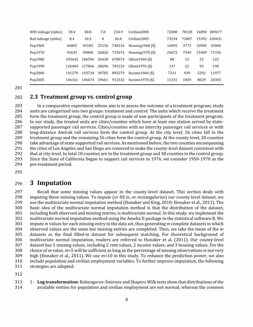
Table 2 presents descriptive statistics of the city-level data. Note that the coefficients of variation 275 for population and civilian employment vary between 0.99 and 2.01; whereas for income, rent, and 276 housing value the coefficients of variation are between 0.13 and 0.31. This suggests that population 277 and income are more dispersed across cities than rent, income, and housing value. 278

279

Table 2: Descriptive statistics of the city-level dataset 280

Variable Mean Std. Dev. Min Max

Variable Mean Std. Dev. Min Max

Land Area (sq miles) 25.4 28.5 3 174.9 Civilian1960 29958 43276 8491 352858

Jan. temp. (°F) 53.9 3.9 46 58.8 Civilian1970 39551 44134 11199 340075

Jul. temp. (°F) 71.2 5 57.3 83.1 Civilian1980 51954 55156 13390 364689

Ann. prec. (inches) 16.1 4.6 6.5 31 Civilian1990 65966 68717 15086 434202

8

NHS mileage (miles) 38.4 40.8 7.8 234.9 Civilian2000 72008 78138 16890 489677

Rail mileage (miles) 8.4 10.3 0 46.8 Civilian2005 73234 72807 15392 430431

Pop1960 46802 94182 25136 740316 Housing1960 ($) 16095 3773 10900 35000

Pop1970 93635 99800 26826 715674 Housing1970 ($) 24672 7549 15409 71336

Pop1980 103642 106596 26438 678974 GRent1960 ($) 88 13 55 122

Pop1990 126404 127866 28696 783233 GRent1970 ($) 137 22 93 190

Pop2000 141270 143718 30785 895279 Income1960 ($) 7221 939 5292 11977

Pop2005 146161 146674 29661 912332 Income1970 ($) 11331 1859 8029 20303

281

2.3 Treatment group vs. control group 282

In a comparative experiment whose aim is to assess the outcome of a treatment program, study 283 units are categorized into two groups: treatment and control. The units which receive the treatment 284 form the treatment group; the control group is made of non-participants of the treatment program. 285 In our study, the treated units are cities/counties which have at least one station served by state-286 supported passenger rail services. Cities/counties with no intercity passenger rail services or with 287 long-distance Amtrak rail services form the control group. At the city level, 26 cities fall in the 288 treatment group and the remaining 56 cities form the control group. At the county level, 20 counties 289 take advantage of state-supported rail services. As mentioned before, the two counties encompassing 290 the cities of Los Angeles and San Diego are removed to make the county-level dataset consistent with 291 that at city-level. In total 18 counties are in the treatment group and 38 counties in the control group. 292 Since the State of California began to support rail services in 1976, we consider 1950-1970 as the 293 pre-treatment period. 294

295

3 Imputation 296

Recall that some missing values appear in the county-level dataset. This section deals with 297 imputing these missing values. To impute (or fill in, or rectangularize) our county-level dataset, we 298 use the multivariate normal imputation method (Honaker and King, 2010; Honaker et al., 2011). The 299 basic idea of the multivariate normal imputation method is that the distribution of the dataset, 300 including both observed and missing entries, is multivariate normal. In this study, we implement the 301 multivariate normal imputation method using the Amelia II package in the statistical software R. We 302 impute m values for each missing entry in the data set, thus generating m complete datasets in which 303 observed values are the same but missing entries are completed. Then, we take the mean of the m 304 datasets as the final filled-in dataset for subsequent matching. For theoretical background of 305 multivariate normal imputation, readers are referred to Honaker et al. (2011). Our county-level 306 dataset has 5 missing values, including 2 rent values, 2 income values, and 3 housing values. For the 307 choice of m value, m=5 will be sufficient as long as the percentage of missing observations is not very 308 high (Honaker et al., 2011). We use m=10 in this study. To enhance the prediction power, we also 309 include population and civilian employment variables. To further improve imputation, the following 310 strategies are adopted: 311

312

1- Log transformation: Kolmogorov-Smirnov and Shapiro-Wilk tests show that distributions of the 313 available entries for population and civilian employment are not normal; whereas the common 314

9

logarithm (i.e., with base 10) of each variable is normally distributed. Therefore, we use the 315 common logarithm of population and civilian employment. 316 317

2- Time-series data: Amelia is capable of identifying time-series patterns of observed data. By 318 estimating a sequence of polynomials of the time index, the package creates a model of patterns 319 within variables across time. Amelia then adds the generated patterns as new covariates to the 320 existing dataset and conducts imputation. The new covariates improve predictability of the 321 imputation model. We will take advantage of this ability in our imputation. 322 323

3- Logical bounds: for each missing value, we provide appropriate lower and upper bounds. For 324 example, the lower and upper bounds for income in a county are set to 0 and income of the next 325 decade. Although sometimes these bounds are not tight, they improve the imputation. 326

327

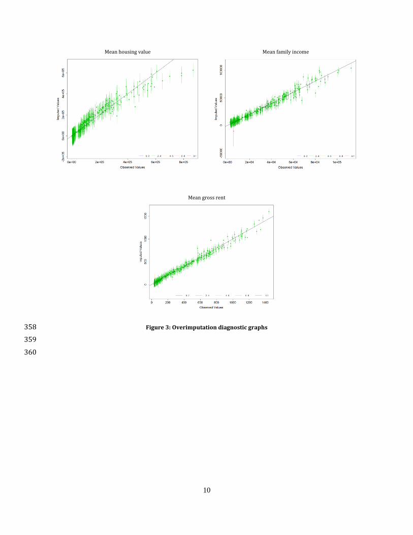
To check the quality of the missing value imputation, we conduct overimputation. In this process, 328 we sequentially assume that one of the observed entries is missing and perform imputation. Imputed 329 values are then plotted against observed values. Imputation would be perfect if all points lie on the 330 45° line of the imputed value – observed value plot. For each observed entry, we impute a large 331 number of values, based on which we construct a 90% confidence interval. Figure 3 shows the 332 confidence intervals on the imputed value – observed value plots for housing value, family income, 333 and gross rent. Most of the intervals are centered around the 45° line, indicating that the multivariate 334 normal imputation method performs well in filling-in missing values for all four variables. Note that 335 a red confidence interval in the plots (i.e., at the lower end of the family income and gross rent plots) 336 indicates that the corresponding observation has fewer covariates available for imputation, resulting 337 in greater variance of the imputed values. 338

The descriptive statistics of the complete county-level dataset are presented in Table 3. We find 339 that values for the population and income variables are more dispersed across counties, with 340 coefficients of variation between 1.3 and 1.6. For income, rent, and housing value, the coefficients of 341 variation are between 0.13 and 0.3. This is in line with the coefficient of variation values at the city 342 level and thus a further validation of the imputed values. 343

344

345

346

347

348

349

350

351

352

353

354

355

356

357

10

Mean housing value

Mean family income

Mean gross rent

Figure 3: Overimputation diagnostic graphs 358

359

360

11

Table 3: Descriptive statistics of the completed county-level dataset 361

Variable Mean Std. dev. Min Max Variable Mean Std. dev. Min Max

Land area (sq miles) 2637.4 3147.2 46.7 20052.5 NHS mileage (miles) 295.3 270.8 64.4 1594.7

Water area (sq miles) 120 177.1 0.5 1052.1 Housing 1950 ($) 7072 2171 3428 12547

Water pct. (%) 7.4 12.8 0.1 75 Housing 1960 ($) 12098 2804 7200 20200

Jan. temp. (°F) 44.1 6.7 28.6 54.2 Housing 1970 ($) 18562 5055 11227 33852

Jul. temp (°F) 71.6 7.6 56.3 92.0 Income 1950 ($) 3263 432 2256 4467

Pop. 1950 104959 154441 241 775357 Income 1960 ($) 5927 782 4438 8110

Pop. 1960 154383 212749 397 908209 Income 1970 ($) 9372 1459 6551 13931

Pop. 1970 206486 303310 484 1420386 Civilian 1950 41261 66285 86 359060

Pop. 1980 255867 371579 1097 1932709 Civilian 1960 58614 85094 129 360427

Pop. 1990 328551 472601 1113 2410556 Civilian 1970 80685 124350 217 575570

Pop. 2000 384616 557150 1208 2846289 Civilian 1980 122828 190468 612 1016754

Pop. 2010 434644 629605 1175 3010232 Civilian 1990 164905 253088 591 1357847

GRent 1950 ($) 39 6 16 56.26 Civilian 2000 182177 270295 683 1409897

GRent 1960 ($) 70 12 33 107 Civilian 2010 216061 319657 604 1592219

GRent 1970 ($) 109 21 73 172

362

Figure 4 illustrates how county-level population, civilian employment over population ratio, 363 income, and housing value, by control vs. treatment group, have evolved between 1950 and 2010. 364 Population, income, and housing value have steadily increased since 1950. Compared to counties 365 with no state-supported Amtrak services (i.e., counties in the control group), average population, 366 income, and housing value are always greater for counties having state-supported services (i.e., 367 counties in the treatment group). This difference is most significant for population. We further 368 observe a diverging trend over time between the treatment and control curves in population, income, 369 and housing values. The lower-right panel shows the county-average value of civil employment over 370 population. For both control and treatment groups, this ratio slightly drops from 1950 to 1960. 371 Greater ratio mostly appears in the treated counties in the post treatment period. 372

373

374

375

376

377

378

379

380

381

382

383

12

Mean population

Mean housing value

Mean income

Mean employment/population

Figure 4: Illustration of population, income, civilian employment/population ratio, 384 and housing value evolution in 1950-2010 385

386

4 Causal inference 387

In general, causal inference in a randomized investigation, in which treatment is randomly 388 assigned to units, is straightforward. Estimation of the treatment effects is given by the difference in 389 the outcome of interest between treated and control units. Unfortunately, Amtrak stations are not 390 randomly assigned to counties and cities. In this case, baseline characteristics, known as baseline 391 covariates, of the treatment group can systematically differ from those of the control group. One 392 approach to correct for this systematic difference in baseline covariates is to use a matching model. 393 In this study, we employ one-to-one propensity score matching methods to draw units from the 394 control group and match them with units from the treatment group. Below we start with the Rubin’s 395 causal inference model (Rubin, 1973; 1974) and the propensity score matching method. We then 396 present the matching results. 397

0

100

200

300

400

500

600

700

800

900

1950 1960 1970 1980 1990 2000 2010

Po

pu

lati

on

(in

th

ou

san

d)

Year

Control Treatment

Pre-tratment Post treatmet

0

50

100

150

200

250

300

350

400

450

1950 1960 1970 1980 1990 2000 2010

Ho

usi

ng

va

lue

($

00

0)

Year

Control Treatment

Pre-tratment Post treatment

0

10

20

30

40

50

60

70

1950 1960 1970 1980 1990 2000 2010

Inco

me

($

00

0)

Year

Control Treatment

Pre-treatment Post treatment

0.37

0.39

0.41

0.43

0.45

0.47

0.49

0.51

0.53

0.55

1950 1960 1970 1980 1990 2000 2010

Civ

ilia

n e

mp

loy

me

nt/

po

pu

lati

on

Year

Control Treatment

Pre-treatment Post treatment

13

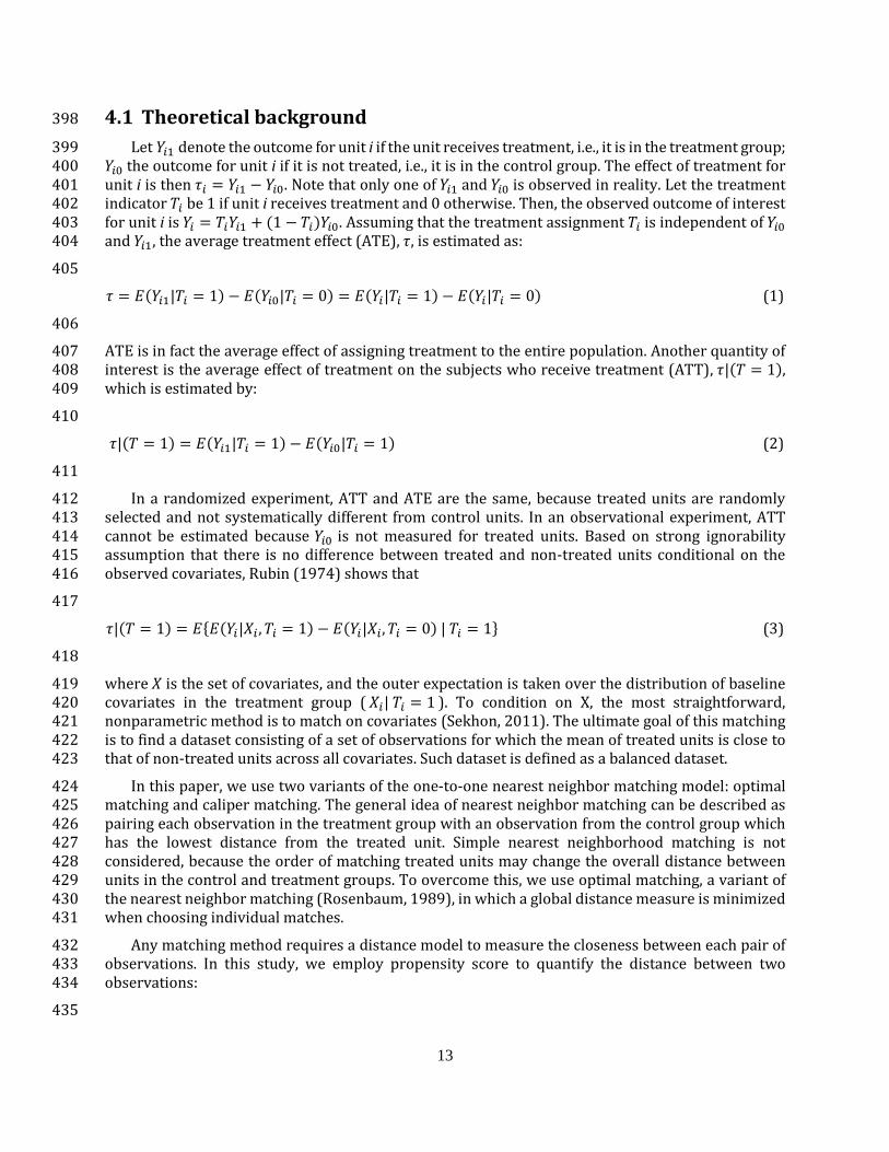
4.1 Theoretical background 398

Let 𝑌𝑖1 denote the outcome for unit i if the unit receives treatment, i.e., it is in the treatment group; 399 𝑌𝑖0 the outcome for unit i if it is not treated, i.e., it is in the control group. The effect of treatment for 400 unit i is then 𝜏𝑖 = 𝑌𝑖1 − 𝑌𝑖0. Note that only one of 𝑌𝑖1 and 𝑌𝑖0 is observed in reality. Let the treatment 401 indicator 𝑇𝑖 be 1 if unit i receives treatment and 0 otherwise. Then, the observed outcome of interest 402 for unit i is 𝑌𝑖 = 𝑇𝑖𝑌𝑖1 + (1 − 𝑇𝑖)𝑌𝑖0. Assuming that the treatment assignment 𝑇𝑖 is independent of 𝑌𝑖0 403 and 𝑌𝑖1, the average treatment effect (ATE), 𝜏, is estimated as: 404

405

𝜏 = 𝐸(𝑌𝑖1|𝑇𝑖 = 1) − 𝐸(𝑌𝑖0|𝑇𝑖 = 0) = 𝐸(𝑌𝑖|𝑇𝑖 = 1) − 𝐸(𝑌𝑖|𝑇𝑖 = 0) (1)

406

ATE is in fact the average effect of assigning treatment to the entire population. Another quantity of 407 interest is the average effect of treatment on the subjects who receive treatment (ATT), 𝜏|(𝑇 = 1), 408 which is estimated by: 409

410

𝜏|(𝑇 = 1) = 𝐸(𝑌𝑖1|𝑇𝑖 = 1) − 𝐸(𝑌𝑖0|𝑇𝑖 = 1) (2)

411

In a randomized experiment, ATT and ATE are the same, because treated units are randomly 412 selected and not systematically different from control units. In an observational experiment, ATT 413 cannot be estimated because 𝑌𝑖0 is not measured for treated units. Based on strong ignorability 414 assumption that there is no difference between treated and non-treated units conditional on the 415 observed covariates, Rubin (1974) shows that 416

417

𝜏|(𝑇 = 1) = 𝐸{𝐸(𝑌𝑖|𝑋𝑖 , 𝑇𝑖 = 1) − 𝐸(𝑌𝑖|𝑋𝑖, 𝑇𝑖 = 0) | 𝑇𝑖 = 1} (3)

418

where 𝑋 is the set of covariates, and the outer expectation is taken over the distribution of baseline 419 covariates in the treatment group ( 𝑋𝑖| 𝑇𝑖 = 1 ). To condition on X, the most straightforward, 420 nonparametric method is to match on covariates (Sekhon, 2011). The ultimate goal of this matching 421 is to find a dataset consisting of a set of observations for which the mean of treated units is close to 422 that of non-treated units across all covariates. Such dataset is defined as a balanced dataset. 423

In this paper, we use two variants of the one-to-one nearest neighbor matching model: optimal 424 matching and caliper matching. The general idea of nearest neighbor matching can be described as 425 pairing each observation in the treatment group with an observation from the control group which 426 has the lowest distance from the treated unit. Simple nearest neighborhood matching is not 427 considered, because the order of matching treated units may change the overall distance between 428 units in the control and treatment groups. To overcome this, we use optimal matching, a variant of 429 the nearest neighbor matching (Rosenbaum, 1989), in which a global distance measure is minimized 430 when choosing individual matches. 431

Any matching method requires a distance model to measure the closeness between each pair of 432 observations. In this study, we employ propensity score to quantify the distance between two 433 observations: 434

435

14

𝐷𝑖𝑗 = 𝑒𝑖 − 𝑒𝑗 (4)

436

where 𝐷𝑖𝑗 is the distance between observation i and observation j; and 𝑒𝑘 (𝑘 = 𝑖, 𝑗) is the propensity 437

score for observation k. Propensity score for observation k is the probability of being treated: 438 𝑒𝑘(𝑋𝑘) = 𝑃𝑟(𝑇𝑘 = 1|𝑋𝑘) . In fact, propensity score summarizes the values of all covariates for 439 observation k (i.e., 𝑋𝑘) into one scalar (𝑒𝑘), i.e., the probability of being treated. If observation j (from 440 the control group) is perfectly matched with observation i (from the treatment group), it means that 441 𝑒𝑗 = 𝑒𝑖 . Any model relating a binary variable, i.e., the variable indicating if an observation received 442

treatment (𝑇), to a set of covariates (X) can be employed to estimate propensity score. In this study, 443 we use logistic regression to estimate propensity scores. 444

When optimal matching results in poor matches, i.e., large distances between observations of 445 each matched pair, one remedy is to impose a caliper. In doing so, we only select a matched pair if it 446 is within a pre-specified caliper: 447

448

|𝑒𝑖 − 𝑒𝑗| ≤ 𝛿 (5)

449

where 𝛿 is the width of the caliper. This width is usually set to a multiplier of standard deviation of 450 propensity scores across all observations. In this study, we use caliper matching with a 0.3 standard 451 deviation of propensity score used for city-level data. At the county level, however, we still stick to 452 optimal matching because imposing a caliper excludes most observations and leaves very few match 453 pairs for regression. 454

To examine how well the matching model balances the treatment and control groups, we use the 455 standardized difference of means (SDM): 456

457

𝑆𝐷𝑀 =�̅�𝑡 − �̅�𝑐

𝜎𝑡 (6)

458

where, �̅�𝑡 is the mean of covariates in the treatment group; �̅�𝑐 the mean of covariates in the control 459 group; and 𝜎𝑡 the standard deviation of covariates in the treatment group. We compute standardized 460 difference of means before and after matching. Percentage of balance improvement (PBI) is then 461 defined as: 462

463

𝑃𝐵𝐼 =|𝑆𝐷𝑀𝐵𝑒𝑓𝑜𝑟𝑒| − |𝑆𝐷𝑀𝐴𝑓𝑡𝑒𝑟|

|𝑆𝐷𝑀𝐵𝑒𝑓𝑜𝑟𝑒|∗ 100% (7)

464

4.2 Results 465

We use the MatchIt package in R to implement optimal and caliper matching models (Ho et al., 466 2007). Recall that the State of California began to support rail services in 1976, we consider 1950-467 1970 as the pre-treatment period. The first step in implementing a matching model is to determine 468 what variables to be included. The key concept in this inclusion is strong ignorability assumption. To 469

15

best satisfy this assumption, it is suggested that analysts be liberal in including potentially associated 470 variables and add as many as possible variables which have some relevance to both the treatment 471 assignment and the outcome of interest (Stuart, 2010). This is because when using a propensity score 472 matching model, inclusion of a variable that is not so relevant to the outcome variable may only 473 slightly increase the variance of other covariates among matched control units. But ignoring a 474 variable that has close relevance to the outcome variable can substantially elevate the bias (Stuart, 475 2010). 476

At the county level, we match on the natural logarithm of population in 1950-1970, housing value 477 in 1950-1970, percentage of land in total area, the presence of a reachable airport, the presence of a 478 port, mean January temperature, and NHS mileage. To account for population and housing growth 479 rates (i.e., 1950-1960 and 1960-1970), we follow McGraw (2014) and incorporate interaction terms 480 into the matching models. In generating the matching model for total civilian employment, log of 481 civilian employment replaces log of population. This set of covariates covers a wide range of county 482 socioeconomic, geographic, climate, and transportation characteristics. At the same time, it results in 483 the highest possible balance improvement across most covariates. 484

Table 4 documents standardized difference of means before and after matching at the county 485 level. For population matching, we observe that the model substantially improves the balance across 486 all the variables. On average, matching improves the balance across the variables by about 63%. For 487 civilian employment matching model, log of NHS mileage results in very poor balance; thus we match 488 on NHS mileage. The highest balance improvements are achieved for housing variables. The average 489 balance improvement across all variables is by about 50.3%. 490

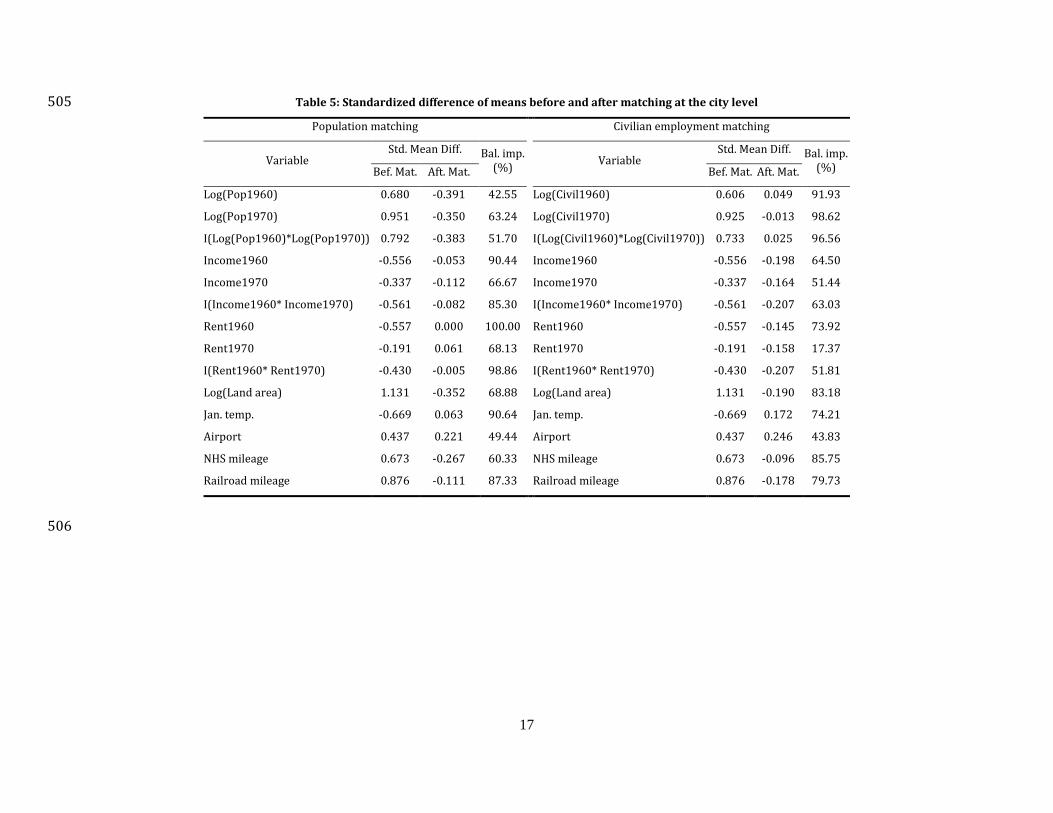
Table 5 shows standardized difference of means before and after matching at the city level. We 491 match on pre-treatment population, mean January temperature, NHS mileage, land area, total freight 492 railroad mileage, the presence of a reachable airport, median gross rent, and median family income. 493 We prefer median gross rent to mean housing value as a covariate in matching because median gross 494 rent results in greater balance improvements. We include median family income so that the number 495 of covariates of city-level matching is comparable to county-level matching. On average, matching 496 improves SDM of population and civilian employment by 73% and 70% respectively. 497

498

499

500

501

16

Table 4: Standardized difference of means before and after matching at the county level 502

Population matching Civilian employment matching

Variable Std. Mean Diff. Bal. imp.

(%)

Variable

Std. Mean Diff. Bal. imp. (%) Bef. Mat. Aft. Mat. Bef. Mat. Aft. Mat.

Log(Pop1950) 1.890 0.638 66.24 Log(Civil1950) 1.791 1.149 35.86

Log(Pop1960) 1.861 0.653 64.92 Log(Civil1960) 1.741 1.071 38.48

Log(Pop1970) 1.849 0.689 62.77 Log(Civil1970) 1.719 1.058 38.44

I(Log(Pop1950)*Log(Pop1960)) 1.683 0.614 63.51 I(Log(Civil1950)*Log(Civil1960)) 1.570 1.021 34.99

I(Log(Pop1960)*Log(Pop1970)) 1.656 0.637 61.51 I(Log(Civil1960)*Log(Civil1970)) 1.534 0.975 36.44

House1950 0.825 0.216 73.82 House1950 0.825 0.403 51.16

House1960 0.469 0.067 85.63 House1960 0.469 0.051 89.09

House1970 0.221 -0.047 78.88 House1970 0.221 0.017 92.11

I(House1950*House1960) 0.581 0.063 89.12 I(House1950*House1960) 0.581 0.193 66.86

I(House1960*House1970) 0.294 -0.063 78.69 I(House1960*House1970) 0.294 -0.032 89.11

Port 0.335 0.130 61.22 Port 0.335 0.260 22.45

Airport 0.940 0.458 51.28 Airport 0.940 0.573 39.10

Jan. temp. 1.471 0.391 73.43 Log (Jan. temp.) 1.782 0.683 61.64

Log(Land area) -0.084 0.076 8.86 Log(Land area) -0.084 -0.066 21.50

Log(NHS mileage) 0.999 0.738 26.11 NHS mileage 0.598 0.380 36.54

503

504

17

Table 5: Standardized difference of means before and after matching at the city level 505

Population matching Civilian employment matching

Variable Std. Mean Diff. Bal. imp.

(%) Variable

Std. Mean Diff. Bal. imp. (%) Bef. Mat. Aft. Mat. Bef. Mat. Aft. Mat.

Log(Pop1960) 0.680 -0.391 42.55 Log(Civil1960) 0.606 0.049 91.93

Log(Pop1970) 0.951 -0.350 63.24 Log(Civil1970) 0.925 -0.013 98.62

I(Log(Pop1960)*Log(Pop1970)) 0.792 -0.383 51.70 I(Log(Civil1960)*Log(Civil1970)) 0.733 0.025 96.56

Income1960 -0.556 -0.053 90.44 Income1960 -0.556 -0.198 64.50

Income1970 -0.337 -0.112 66.67 Income1970 -0.337 -0.164 51.44

I(Income1960* Income1970) -0.561 -0.082 85.30 I(Income1960* Income1970) -0.561 -0.207 63.03

Rent1960 -0.557 0.000 100.00 Rent1960 -0.557 -0.145 73.92

Rent1970 -0.191 0.061 68.13 Rent1970 -0.191 -0.158 17.37

I(Rent1960* Rent1970) -0.430 -0.005 98.86 I(Rent1960* Rent1970) -0.430 -0.207 51.81

Log(Land area) 1.131 -0.352 68.88 Log(Land area) 1.131 -0.190 83.18

Jan. temp. -0.669 0.063 90.64 Jan. temp. -0.669 0.172 74.21

Airport 0.437 0.221 49.44 Airport 0.437 0.246 43.83

NHS mileage 0.673 -0.267 60.33 NHS mileage 0.673 -0.096 85.75

Railroad mileage 0.876 -0.111 87.33 Railroad mileage 0.876 -0.178 79.73

506

18

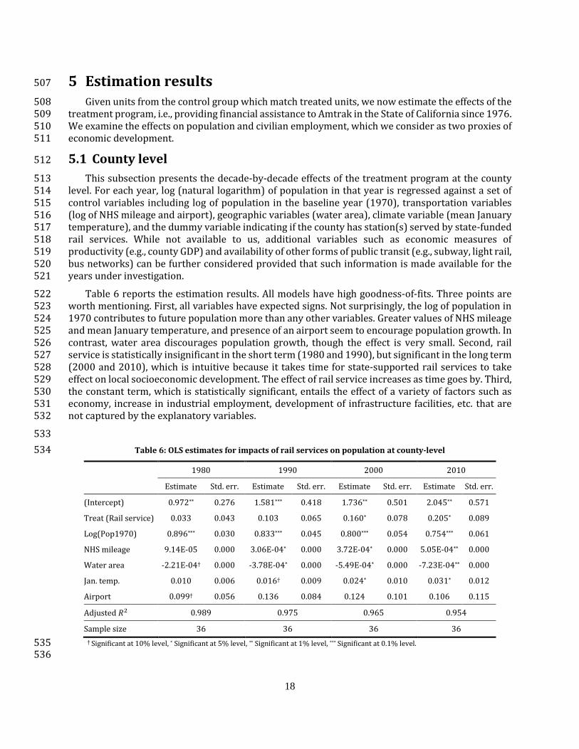
5 Estimation results 507

Given units from the control group which match treated units, we now estimate the effects of the 508 treatment program, i.e., providing financial assistance to Amtrak in the State of California since 1976. 509 We examine the effects on population and civilian employment, which we consider as two proxies of 510 economic development. 511

5.1 County level 512

This subsection presents the decade-by-decade effects of the treatment program at the county 513 level. For each year, log (natural logarithm) of population in that year is regressed against a set of 514 control variables including log of population in the baseline year (1970), transportation variables 515 (log of NHS mileage and airport), geographic variables (water area), climate variable (mean January 516 temperature), and the dummy variable indicating if the county has station(s) served by state-funded 517 rail services. While not available to us, additional variables such as economic measures of 518 productivity (e.g., county GDP) and availability of other forms of public transit (e.g., subway, light rail, 519 bus networks) can be further considered provided that such information is made available for the 520 years under investigation. 521

Table 6 reports the estimation results. All models have high goodness-of-fits. Three points are 522 worth mentioning. First, all variables have expected signs. Not surprisingly, the log of population in 523 1970 contributes to future population more than any other variables. Greater values of NHS mileage 524 and mean January temperature, and presence of an airport seem to encourage population growth. In 525 contrast, water area discourages population growth, though the effect is very small. Second, rail 526 service is statistically insignificant in the short term (1980 and 1990), but significant in the long term 527 (2000 and 2010), which is intuitive because it takes time for state-supported rail services to take 528 effect on local socioeconomic development. The effect of rail service increases as time goes by. Third, 529 the constant term, which is statistically significant, entails the effect of a variety of factors such as 530 economy, increase in industrial employment, development of infrastructure facilities, etc. that are 531 not captured by the explanatory variables. 532

533

Table 6: OLS estimates for impacts of rail services on population at county-level 534

1980 1990 2000 2010

Estimate Std. err. Estimate Std. err. Estimate Std. err. Estimate Std. err.

(Intercept) 0.972** 0.276 1.581*** 0.418 1.736** 0.501 2.045** 0.571

Treat (Rail service) 0.033 0.043 0.103 0.065 0.160* 0.078 0.205* 0.089

Log(Pop1970) 0.896*** 0.030 0.833*** 0.045 0.800*** 0.054 0.754*** 0.061

NHS mileage 9.14E-05 0.000 3.06E-04* 0.000 3.72E-04* 0.000 5.05E-04** 0.000

Water area -2.21E-04† 0.000 -3.78E-04* 0.000 -5.49E-04* 0.000 -7.23E-04** 0.000

Jan. temp. 0.010 0.006 0.016† 0.009 0.024* 0.010 0.031* 0.012

Airport 0.099† 0.056 0.136 0.084 0.124 0.101 0.106 0.115

Adjusted 𝑅2 0.989 0.975 0.965 0.954

Sample size 36 36 36 36

† Significant at 10% level, * Significant at 5% level, ** Significant at 1% level, *** Significant at 0.1% level. 535 536

19

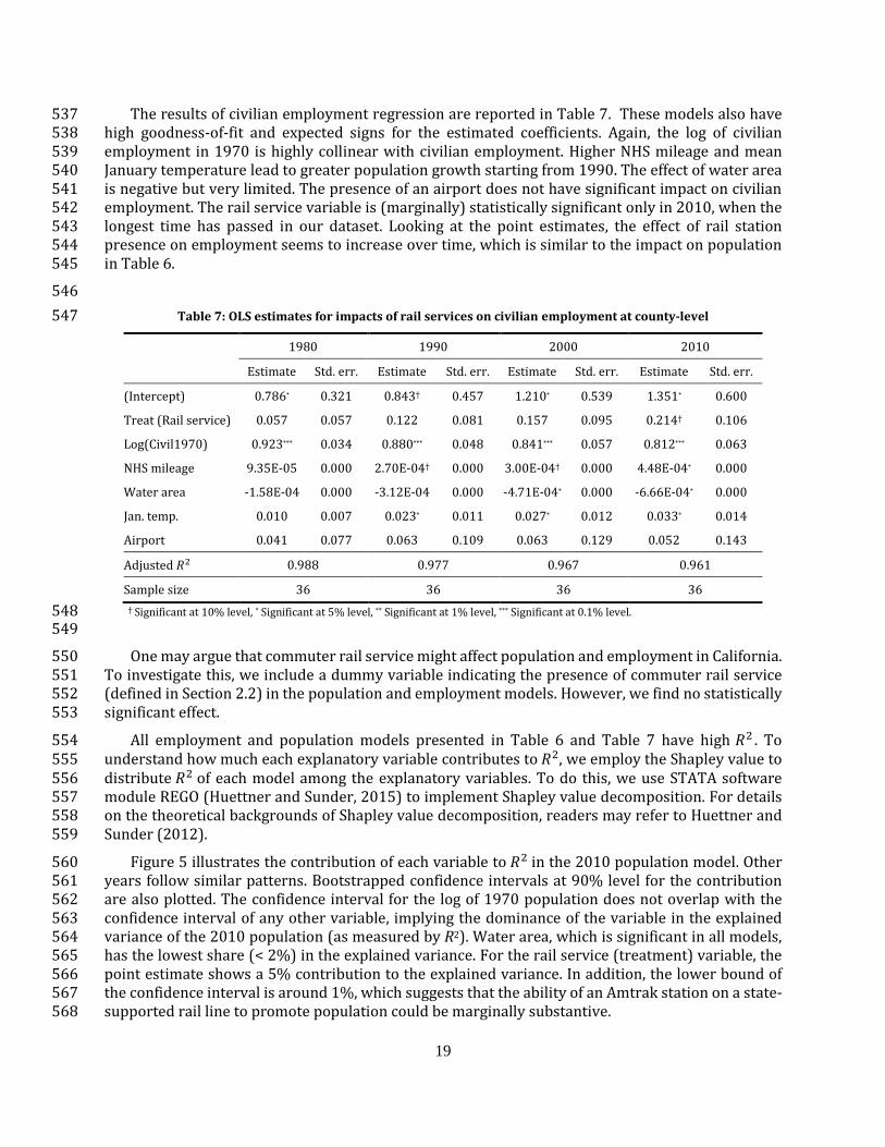
The results of civilian employment regression are reported in Table 7. These models also have 537 high goodness-of-fit and expected signs for the estimated coefficients. Again, the log of civilian 538 employment in 1970 is highly collinear with civilian employment. Higher NHS mileage and mean 539 January temperature lead to greater population growth starting from 1990. The effect of water area 540 is negative but very limited. The presence of an airport does not have significant impact on civilian 541 employment. The rail service variable is (marginally) statistically significant only in 2010, when the 542 longest time has passed in our dataset. Looking at the point estimates, the effect of rail station 543 presence on employment seems to increase over time, which is similar to the impact on population 544 in Table 6. 545

546

Table 7: OLS estimates for impacts of rail services on civilian employment at county-level 547

1980 1990 2000 2010


(Intercept) 0.786* 0.321 0.843† 0.457 1.210* 0.539 1.351* 0.600

Treat (Rail service) 0.057 0.057 0.122 0.081 0.157 0.095 0.214† 0.106

Log(Civil1970) 0.923*** 0.034 0.880*** 0.048 0.841*** 0.057 0.812*** 0.063

NHS mileage 9.35E-05 0.000 2.70E-04† 0.000 3.00E-04† 0.000 4.48E-04* 0.000

Water area -1.58E-04 0.000 -3.12E-04 0.000 -4.71E-04* 0.000 -6.66E-04* 0.000

Jan. temp. 0.010 0.007 0.023* 0.011 0.027* 0.012 0.033* 0.014

Airport 0.041 0.077 0.063 0.109 0.063 0.129 0.052 0.143

Adjusted 𝑅2 0.988 0.977 0.967 0.961



One may argue that commuter rail service might affect population and employment in California. 550 To investigate this, we include a dummy variable indicating the presence of commuter rail service 551 (defined in Section 2.2) in the population and employment models. However, we find no statistically 552 significant effect. 553

All employment and population models presented in Table 6 and Table 7 have high 𝑅2 . To 554 understand how much each explanatory variable contributes to 𝑅2, we employ the Shapley value to 555 distribute 𝑅2 of each model among the explanatory variables. To do this, we use STATA software 556 module REGO (Huettner and Sunder, 2015) to implement Shapley value decomposition. For details 557 on the theoretical backgrounds of Shapley value decomposition, readers may refer to Huettner and 558 Sunder (2012). 559

Figure 5 illustrates the contribution of each variable to 𝑅2 in the 2010 population model. Other 560 years follow similar patterns. Bootstrapped confidence intervals at 90% level for the contribution 561 are also plotted. The confidence interval for the log of 1970 population does not overlap with the 562 confidence interval of any other variable, implying the dominance of the variable in the explained 563 variance of the 2010 population (as measured by R2). Water area, which is significant in all models, 564 has the lowest share (< 2%) in the explained variance. For the rail service (treatment) variable, the 565 point estimate shows a 5% contribution to the explained variance. In addition, the lower bound of 566 the confidence interval is around 1%, which suggests that the ability of an Amtrak station on a state-567 supported rail line to promote population could be marginally substantive. 568

20

569

Figure 5: Decomposition of R2 for 2010 county population model, with 90% bootstrap 570 confidence interval, based on 5000 bootstrap replications 571

572

In an attempt to further testify the effect of state financial support for Amtrak passenger rail 573 services on local population and employment, we also collect data and perform similar analysis for 574 another state, Illinois. Details about the data collection, matching, and regression are presented in 575 the Appendix. The results show that, like the California case, state support for Amtrak passenger rail 576 services has statistically significant effects on population and employment only in part of the years. 577 Compared to the California case, however, the effects are generally small and in short term, which 578 might be attributed to different strengths of support of the two states over time. 579

5.2 City level 580

This subsection presents the estimated impact on city-level population and civil employment of 581 Amtrak stations on state-supported rail lines. There are two differences in the choice of explanatory 582 variables between the city- and county-level models. First, we use land area, which is expected to 583 have the opposite effect of water area (in fact, the water area variable is not available at the city level). 584 Second, since all cities in the dataset have a reachable airport located in less than 50 miles from the 585 city’s boundary, we do not include an airport variable. 586

Table 8 reports the estimated results for the population model. As expected, population in 1970 587 is still highly significant, although the coefficient suggests that the impact is smaller than at the county 588 level. The coefficients for NHS mileage are positive and statistically significant across all four models. 589 However, neither the land area nor the January temperature variable has a significant effect on 590 population. 591

Turning to the treatment variable, we find that the presence of an Amtrak station on a state-592 supported line does not have significant effect on population in 1980; however, the effect becomes 593 significant starting from 1990. The magnitude of the point estimate is similar to the county-level 594 estimate: forty years after the establishment of the state support (2010), an Amtrak station on a state-595 supported line increases a city’s population by 17%. 596

597

598

0.00 0.10 0.20 0.30 0.40 0.50 0.60

Rail service

Log(Pop1970)

NHS mileage

Water area

Jan. temp.

Airport

Absolute contribution to R2

21

Table 8: OLS estimates for impacts of rail services on population at city-level 599

1980 1990 2000 2005


(Intercept) 2.158 1.351 2.955 1.969 2.793 2.082 2.435 2.290

Treat (Rail service) 0.087 0.053 0.146† 0.077 0.180* 0.082 0.170† 0.090

Log(Pop1970) 0.738*** 0.078 0.570*** 0.113 0.487** 0.120 0.445** 0.132

Log(NHS Mileage) 0.283** 0.090 0.483** 0.132 0.561** 0.139 0.569** 0.153

Land area 8.38E-04 0.003 2.04E-03 0.004 2.28E-03 0.004 4.40E-03 0.004

Log(Jan. temp.) -0.037 0.387 0.100 0.564 0.325 0.597 0.522 0.656

Adjusted 𝑅2 0.942 0.894 0.887 0.875



Estimates for the civilian employment models are documented in Table 9. Compared to the 602 population models, the civilian employment models have lower 𝑅2 values. Again, land area and 603 January temperature variables do not have significant coefficients. As in the county-level models, 604 civilian employment in 1970 and NHS mileage have positive coefficients, which are mostly significant. 605 We find that the coefficients of the treatment variable are statistically insignificant in all four models. 606 This confirms the finding at the county level that the presence of an Amtrak station on a state-607 supported line has little effect on civilian employment. 608

Similar to the county-level case, we investigate the impact of commuter rail service on population 609 and employment at the city level. Again, the estimates are not statistically significant. 610

611

Table 9: OLS estimates for impacts of rail services on civilian employment at city-level 612

1980 1990 2000 2005


(Intercept) 2.973 2.734 4.477 2.925 5.854† 2.998 3.850 2.759

Treat (Rail service) 0.001 0.080 0.0170 0.085 0.047 0.087 0.059 0.081

Log(Civil1970) 0.826*** 0.137 0.653*** 0.147 0.669*** 0.150 0.597** 0.138

Log(NHS Mileage) 0.170 0.111 0.300* 0.119 0.251† 0.122 0.282* 0.112

Land area -2.71E-04 0.003 1.78E-03 0.004 2.69E-03 0.004 5.93E-03 0.003

Log(Jan. temp.) -0.368 0.628 -0.363 0.672 -0.702 0.689 -0.049 0.634

Adjusted 𝑅2 0.838 0.842 0.825 0.877



We also investigate how much each of the explanatory variables contributes to R2 in the 615 population model. We do not present the results for the civilian employment models, as the treatment 616 variable is not significant. Figure 6 shows the R2 decomposition results for the 2005 city population 617 model. Again, models for other years offer similar results. As in the county-level case, the baseline 618 population and NHS mileage have the greatest mean contributions to R2, with about 40% and 32% 619

22

shares respectively. The treatment variable contributes about 2% to the explained variance. The 620 wide confidence interval of the treatment variable, in particular the lower bound which is again close 621 to 1%, reaffirms our earlier argument at the county level that the effect on population of an Amtrak 622 station on a state-supported rail line could be small. 623

624

625

Figure 6: Decomposition of R2 for the 2005 city population model, 626

with 90% bootstrap confidence interval, based on 5000 bootstrap replications 627

628

6 Concluding remarks 629

Passenger rail played a vital role in US intercity travel and economy in the early 20th century. 630 However, due to the advent of automobiles and airplanes, passenger rail lost much of its dominance. 631 The establishment of Amtrak in 1971 and subsequently state-level support for parts of Amtrak’s 632 services helped preserve the passenger rail system in the country and revitalize services that remain 633 an integral part in the national multimodal transportation system. Given that the local socioeconomic 634 impact of such services is largely unknown in the literature, this paper intends to fill the gap by 635 empirically investigating how Amtrak stations on state-support rail lines have affected population 636 and employment at county and city levels. 637

We compile two panel datasets for the state of California which include various county- and city-638 level geographic, transportation, and socioeconomic characteristics. In view of the missing values in 639 the datasets, multivariate normal imputation is used to fill in the missing values. We then employ a 640 propensity score based one-to-one matching model to draw units from the control group, which are 641 counties/cities that do not have a state-supported Amtrak station, to match with units from the 642 treatment group, which are counties/cities that do. Using the matched data, we perform ordinary 643 least square regressions to estimate the effect of a state-supported Amtrak station on local 644 population and employment. 645

The estimation results suggest a positive effect on population at both city and county levels. The 646 effect is more prominent as time goes by. The population growth in turn spurs Amtrak’s ridership, 647 whose growth is more than double the population growth between 2009 and 2015 in the state 648 (Amtrak, 2015). At the county level, the effects on population and civilian employments have similar 649 point estimates. However, for the effect on civilian employment most of them are statistically 650 insignificant (only significant at 10% level in 2010). At the city level, the point estimates for the 651

0.00 0.10 0.20 0.30 0.40 0.50

Treat

Log(Pop1970)

Log(NHS Mile)

Land area

Log(Jan. temp.)

Absolute contribution to R2

23

civilian employment effect are much smaller than for the population effect, and none of them is found 652 statistically significant. 653

Thus overall, we are more confident about the role an average Amtrak station on a state-funded 654 line plays to promote population growth than to encourage civilian employment, although the effect 655 on population growth could still be small, given the confidence intervals of the rail service variable’s 656 contribution to the overall goodness-of-fit of the population models. One plausible explanation may 657 be that state-supported Amtrak services provide quality mobility and accessibility by rail, which 658 attract people to live in rail-accessible regions. On the other hand, the weak effect on employment of 659 state-supported Amtrak service is not surprising, with two possible explanations. First, a train station 660 has only marginal impact on overall accessibility, and therefore can induce limited direct or indirect 661 economic activities. Second, although Amtrak is reported to support thousands of jobs (Amtrak, 662 2015), it is not clear how these jobs are distributed between state-supported and non-state-663 supported routes, and among counties and cities. For example, jobs on purchase of supplies and 664 materials are not necessarily correlated with the geographic coverage of transportation service. Thus, 665 it is hard to draw concrete conclusions on the benefits of state-supported Amtrak stations on local 666 employment. 667

This study can be extended in a few directions. First, this study only investigates the effect of 668 state-supported rail service on total employment in aggregate at county and city levels. It would be 669 interesting to examine the impact on specific sectors (e.g., tradable, non-tradable, and transportation 670 sectors). Second, the impact of an Amtrak station on local development may vary with county/city 671 size. Future research may look into the economic impact of state-supported rail services for different 672 county/city sizes. Third, in addition to the state-supported rail service, several other factors, such as 673 fertility rate, mortality rate (life expectancy), and migration, could be responsible for population 674 growth. In the current models, these factors are only implicitly and indirectly captured through the 675 constant, the 1970 population / employment variable, and the error term. Pin-pointing specific 676 factors is challenging. Future efforts should be directed to identifying such factors, collecting relevant 677 data, and testing their effects on population growth. Finally, this study focuses on California. 678 Application of the methodology developed in this study to other states will lend a more 679 comprehensive understanding of the socioeconomic impact of state-supported Amtrak services. Such 680 understanding can help inform future policies and development of intercity passenger rail in the US. 681 For example, as mentioned in Sperry et al. (2013), the understanding can be incorporated into state 682 rail plans and applications for federal grants for passenger rail. The understanding can also be part 683 of the material for public outreach to local community leaders and businesses, and for educating 684 legislators on the socioeconomic impact of Amtrak service as decision are made about 685 continuing/strengthening/reducing the financial support for passenger rail service in California and 686 elsewhere. 687

688

Acknowledgment 689

This research was partially supported by California Department of Transportation (Caltrans). We 690 would like to thank Dr. Marquise McGraw from the University of California at Berkeley for initial 691 discussions, and Professor David Brownstone from the University of California at Irvine and Dr. 692 Joshua Seeherman from the University of California at Berkeley for their helpful comments. The 693 views are those of the authors alone. 694

695

24

Appendix: Analysis for the State of Illinois 696

In this appendix, we present our data collection and modeling efforts for the State of Illinois. 697 Illinois has four state-supported services: Zephyr Service (Chicago – Quincy, receiving state support 698 since 1971), Lincoln Service (Chicago – Springfield – St. Louis, receiving state support since 1973), 699 Illini Service (Chicago – Champaign, receiving state support since 1973), and Hiawatha Service 700 (Chicago – Milwaukee, receiving state support since 1989). As state support for intercity passenger 701 rail services in Illinois started in the early 1970s, we consider 1950-1970 as the pre-treatment period 702 (the same as in California case). 703

Similar to what we do for California, a dataset is developed which contains socioeconomic, 704 demographic, geographic, and transportation information of Illinois counties between 1950 and 705 2010. The locations of Amtrak stations on state-supported routes are obtained from the Illinois 706 Department of Transportation (IDOT, 2017). In total, 24 counties have such Amtrak stations. Cook 707 County, whose county seat is Chicago, is removed from the dataset because of its very different 708 characteristics from other counties in the state. After the removal, the dataset has 23 counties in the 709 treatment group. The state’s remaining 79 counties form the control group. 710

Most of the information for Illinois is obtained from the same data sources as for California (see 711 Section 2.4), except that commuter rail information draws from Metra (2017). No imputation is 712 needed for Illinois as the collected information is complete. Figure A.1 shows the mean population 713 and civilian employment in the control and treatment groups between 1950 and 2010. 714

715

Mean population

Mean civilian employment

Figure A.1: county-level mean population and civilian employment in the control and the treatment groups 716

717

The explanatory variables considered in the regression models are the same as those in the 718 California models, with two differences: 1) the portion of water area in the total area of a county is 719 used rather than the water area itself; 2) two dummy variables related to the Chicago metropolitan 720 area are added. For the water area portion variable, the hypothesis is that a larger portion of water 721 area has a positive effect on local population/employment. This is because in Illinois, unlike in 722 California, population conglomeration outside the Chicago metropolitan area is often nearby rivers 723 (e.g., Mississippi River, Illinois River, Kaskaskia River, Ohio River, Wabash River, Kankakee River). 724

30

50

70

90

110

130

150

1950 1960 1970 1980 1990 2000 2010

Po

pu

lati

on

(in

th

ou

san

ds)

Year

Control Treatment


10

20

30

40

50

60

70

80

1950 1960 1970 1980 1990 2000 2010

Civ

ilia

n e

mp

loy

me

nt

(in

th

ou

san

ds)

Year

Control Treatment


25

Also note that Cook and Lake counties, which are the only two counties in the state bordered with 725 Lake Michigan, are not in the dataset after matching. 726

The two Chicago metro dummies intends to capture the Chicago effect in dominating the state’s 727 population and the suburbanization trend within the metropolitan area. The first dummy (Chicago 728 metro1) takes value 1 if a county is DuPage, Kane, or Will, and 0 otherwise. These counties are in the 729 immediate surroundings of the city of Chicago. The second dummy (Chicago metro2) takes value 1 if 730 a county is from the following list: DeKalb, Grundy, Kendall, and McHenry, and 0 otherwise. These 731 counties are farther away from the city of Chicago but still belong to the metropolitan area according 732 to US Census Bureau (2016). Our hypothesis is that population and employment in these counties – 733 especially those in the outer region of the Chicago metropolitan area – have grown faster than the 734 rest of the state due to the continuous suburbanization after 1970. 735

The regression results for population and employment are presented in Tables A1 and A2. In the 736 population models, the coefficients for the rail service variable consistently have a positive sign, but 737 only significant in 1980. The point estimates are generally smaller than those for California (see Table 738 6). This suggests that the effect of state support for Amtrak service on local population is in shorter 739 term and weaker in Illinois than in California. 740

For the other variables, the log of population in 1970 again contributes most to the variation in 741 future population. The commuter dummy variable has an expected positive coefficient in all models, 742 but only significant in 1990. The coefficients for NHS mileage and water area portion are consistently 743 non-negative as well, significant only for 2010. January temperature and airport presence do not 744 show statistically significant effect on population. The large and significant coefficients for the outer 745 counties of the Chicago metropolitan area (Chicago metro2) suggest stronger population growth in 746 these counties in the study period than in the inner counties (Chicago metro1) and the rest of the 747 state. 748

749

Table A1: OLS estimates for impacts of rail services on population at the county level for Illinois 750

1980 1990 2000 2010


(Intercept) 0.249 0.333 0.425 0.464 1.054 0.685 1.848 0.981

Treat (Rail service) 0.049* 0.021 0.042 0.030 0.049 0.044 0.061 0.063

Log(Civil1970) 0.970*** 0.027 0.945*** 0.037 0.892*** 0.055 0.822*** 0.078

Commuter 0.143 0.094 0.286* 0.130 0.323 0.193 -0.070 0.276

NHS Mileage -8.14E-05 3.30E-04 1.68E-04 4.60E-04 9.13E-04 6.79E-04 0.002† 0.001

Water area portion 2.111 1.257 2.522 1.752 4.267 2.588 7.163† 3.706

Jan. temp. 0.003 0.004 0.004 0.006 -3.76E-04 0.008 -0.006 0.012

Airport 0.019 0.036 0.077 0.051 0.084 0.075 0.128 0.108

Chicago metro1 0.097 0.091 0.098 0.127 0.198 0.188 0.653* 0.269

Chicago metro2 0.170** 0.051 0.280*** 0.071 0.485*** 0.105 0.942*** 0.150

Adjusted 𝑅2 0.996 0.992 0.984 0.970



26

The results for the civil employment model yield similar insights. The rail service dummy is only 753 significant in 1980. The most explanatory power of the models comes from the log of civil 754 employment in 1970. The commuter variable has a positive coefficient, which is significant for 1990. 755 NHS mileage and water area portion again have positive coefficients, significant only for 2010. The 756 Chicago metro2 variable shows strong and significant effect on civil employment. For the coefficients 757 of the other variables, most of them have expected signs but are statistically insignificant (we note 758 that Jan. Temp. has two unexpected negative coefficients. However, they are also highly insignificant). 759

760

Table A2: OLS estimates for impacts of rail services on civilian employment at the county level for Illinois 761

1980 1990 2000 2010


(Intercept) 0.583 0.408 0.782 0.587 1.445† 0.794 1.910† 1.126

Treat (Rail service) 0.066* 0.027 0.054 0.039 0.072 0.053 0.075 0.076

Log(Civil1970) 0.952*** 0.034 0.921*** 0.049 0.862*** 0.067 0.818*** 0.094

Commuter 0.180 0.121 0.314† 0.174 0.339 0.235 -0.100 0.333

NHS Mileage -3.16E-06 4.25E-04 3.78E-04 6.11E-04 1.13E-03 8.26E-04 0.002† 0.001

Water area portion 2.018 1.615 2.584 2.321 4.626 3.137 8.860† 4.451

Jan. temp. 0.001 0.005 0.003 0.008 -0.001 0.010 -0.007 0.015

Airport 0.056 0.048 0.123† 0.069 0.122 0.093 0.128 0.132

Chicago metro1 0.109 0.118 0.125 0.169 0.181 0.229 0.660* 0.325

Chicago metro2 0.180*** 0.065 0.327*** 0.094 0.510*** 0.127 0.989*** 0.180

Adjusted 𝑅2 0.993 0.987 0.978 0.961



764

765

References 766

1. AECOM, 2013. 2013 California State Rail Plan. California Department of Transportation, 767 Sacramento, CA. 768

2. Aschauer, D.A., 1989. Is public expenditure productive? Journal of Monetary Economics 23 (2), 769 177-200. 770

3. Atack, J., Bateman, F., Haines, M., Margo, R.A., 2010. Did railroads induce or follow economic 771 growth. Social Science History 34 (2), 171-197. 772

4. Atack, J., Margo, R.A., 2009. Agricultural Improvements and Access to Rail Transportation: The 773 American Midwest as a Test Case, 1850-1860. National Bureau of Economic Research, Report No. 774 w15520. 775

5. Banerjee, A., Duflo, E., Qian, N., 2012. On the road: Access to transportation infrastructure and 776 economic growth in China. National Bureau of Economic Research, Report No. w17897. 777

6. Baum-Snow, N., 2007. Did highways cause suburbanization? The Quarterly Journal of Economics 778 122 (2), 775-805. 779

27

7. Berger, T., Enflo, K., 2014. Locomotives of Local Growth: The Short-and Long-Term Impact of 780 Railroads in Sweden. Department of Economic History, Lund University, Repot No. 132. 781

8. Blonigen, B.A., Cristea, A.D., 2015. Air service and urban growth: Evidence from a quasi-natural 782 policy experiment. Journal of Urban Economics 86, 128-146. 783

9. Brueckner, J.K., 2003. Airline traffic and urban economic development. Urban Studies 40 (8), 784 1455-1469. 785

10. Caltrans, 2015. Caltrans GIS Data Library. Available at 786 http://www.dot.ca.gov/hq/tsip/gis/datalibrary/, Retrieved on December 29, 2015. 787

11. Chi, G., 2010. The impacts of highway expansion on population change: An integrated spatial 788 approach. Rural Sociology 75 (1), 58-89. 789

12. Cidell, J., 2015. The role of major infrastructure in subregional economic development: an 790 empirical study of airports and cities. Journal of Economic Geography 15 (6), 1125-1144. 791

13. CTA, 2003. CTA Railroad Network. Available at http://www-792 cta.ornl.gov/transnet/RailRoads.html, Retrieved on December 29, 2015. 793

14. Donaldson, D., Hornbeck, R., 2013. Railroads and American Economic Growth: A" Market Access" 794 Approach. National Bureau of Economic Research, Report No. w19213. 795

15. Duranton, G., Morrow, P.M., Turner, M.A., 2014. Roads and Trade: Evidence from the US. The 796 Review of Economic Studies 81 (2), 681-724. 797

16. Duranton, G., Turner, M.A., 2012. Urban growth and transportation. The Review of Economic 798 Studies 79 (4), 1407-1440. 799

17. Elkind, E.N., Chan, M. Faber, T.V., 2015. Grading California's Rail Transit Station Areas: A Ranking 800 of How Well They Accommodate Population Growth, Boost Economic Activity and Improve the 801 Environment. Center for Law, Energy & the Environment, University of California, Berkeley. 802

18. Faber, B., 2014. Trade integration, market size, and industrialization: evidence from China's 803 National Trunk Highway System. The Review of Economic Studies 81 (3), 1046-1070. 804

19. Franch, X., Morillas-Torné, M., Martí-Henneberg, J., 2013. Railways as a Factor of Change in the 805 Distribution of Population in Spain, 1900–1970. Historical Methods: A Journal of Quantitative and 806 Interdisciplinary History 46 (3), 144-156. 807

20. Garcia-Milà, T., Montalvo, J.G., 2007. The impact of new highways on business location: new 808 evidence from Spain. Centre De Recerca En Economia Internacional, Universitat Pompeu Fabra, 809 working paper. 810

21. Gibbons, S., Lyytikainen, T., Overman, H.G., Sanchis-Guarner, R., 2012. New road infrastructure: 811 the effects on firms. SERC Discussion Papers, SERCDP117. Spatial Economics Research Centre 812 (SERC), London School of Economics and Political Science, London, UK. 813

22. Green, R.K., 2007. Airports and economic development. Real Estate Economics 35 (1), 91-112. 814 23. Gregory, I.N. Henneberg, J.M., 2010. The Railways, Urbanization, and Local Demography in 815

England and Wales. Social Science History 34 (2), 199-228. 816 24. Ho, D., Imai, K., King, G., Stuart, E., 2007. MatchIt: MatchIt: Nonparametric Preprocessing for 817

Parametric Casual Inference. Political Analysis 15 (3), 199-236. 818 25. Honaker, J., King, G., 2010. What to do about missing values in time‐series cross‐section data. 819

American Journal of Political Science 54 (2), 561-581. 820 26. Honaker, J., King, G., Blackwell, M., 2011. Amelia II: A program for missing data. Journal of 821

Statistical Software 45 (7), 1-47. 822 27. Hornung, E., 2012. Railroads and Micro-Regional Growth in Prussia, ifo Institut – Leibniz-Institut 823

für Wirtschaftsforschung an der Universität München, working paper. 824 28. Huettner, F., Sunder, M., 2015. [. rego] R-Squared decomposition. Available at http://www.uni-825

leipzig.de/~rego/, Retrieved on December 29, 2015. 826 29. Huettner, F., Sunder, M., 2012. Axiomatic arguments for decomposing goodness of fit according 827

to Shapley and Owen values. Electronic Journal of Statistics 6, 1239-1250. 828

28

30. ICPSR, 2015a. County and City Data Book [United States] Series. Available at: 829 http://www.icpsr.umich.edu/icpsrweb/ICPSR/series/23, Retrieved on December 29, 2015. 830

31. ICPSR, 2015b. County Characteristics, 2000-2007 [United States] (ICPSR 20660). Available at: 831 http://www.icpsr.umich.edu/icpsrweb/DSDR/studies/20660, Retrieved on December 29, 832 2015. 833

32. IDOT, 2017. Passenger Rail Services. Available at http://www.idot.illinois.gov/travel-834 information/passenger-services/AMTRAK-services/index, Retrieved on October 23, 2017. 835

33. King, G., Honaker, J., Joseph, A., Scheve, K., 2001. Analyzing incomplete political science data: An 836 alternative algorithm for multiple imputation. American Political Science Association 95 (1), 49-837 69. 838

34. Koopmans, C., Rietveld, P., Huijg, A., 2012. An accessibility approach to railways and municipal 839 population growth, 1840–1930. Journal of Transport Geography 25, 98-104. 840

35. Lee, K.J., Carlin, J.B., 2010. Multiple imputation for missing data: fully conditional specification 841 versus multivariate normal imputation. American Journal of Epidemiology 171 (5), 624-632. 842

36. Lieshout, R., 2012. Measuring the size of an airport’s catchment area. Journal of Transport 843 Geography 25, 27-34. 844

37. Marcucci, E. Gatta, V., 2011. Regional airport choice: consumer behaviour and policy implications. 845 Journal of Transport Geography 19 (1), 70-84. 846

38. McGraw, M., 2014. Perhaps the Sky’s the Limit? Airports and Employment in Local Economies. 847 University of California, Berkeley, Job Market paper. 848

39. Metra, 2017. Maps and Schedules | Metra. Available at https://metrarail.com/maps-schedules, 849 Retrieved on October 23, 2017. 850

40. Michaels, G., 2008. The effect of trade on the demand for skill: Evidence from the interstate 851 highway system. The Review of Economics and Statistics 90 (4), 683-701. 852

41. MPC, 2011. National historical geographic information system: Version 2.0. Minnesota 853 Population Center, University of Minnesota, Minneapolis, MN. 854

42. Mukkala, K., Tervo, H., 2013. Air transportation and regional growth: which way does the 855 causality run? Environment and Planning A 45(6), 1508-1520. 856

43. Munnell, A.H., Cook, L.M., 1990. How does public infrastructure affect regional economic 857 performance? New England Economic Review, 11-33. 858

44. Murakami, J., Cervero, R., 2010. California high-speed rail and economic development: Station-859 area market profiles and public policy responses. University of California Transportation Center. 860

45. Nice, D., 1998. The History and Politics of a National Railroad. Lynne Rienner Publishers, Boulder, 861 Colorado. 862

46. NOAA, 2012. NOAA’s List of Coastal Counties. Available at: 863 https://www.census.gov/geo/landview/lv6help/coastal_cty.pdf, Retrieved on December 29, 864 2015. 865

47. NOAA, 2000. Ports List. Available at: 866 http://www.ngs.noaa.gov/RSD/coastal/projects/coastal/ports_list.html, Retrieved on 867 December 29, 2015. 868

48. Nordstrom, M., 2015. The Growth Effect: Commuter Rail in Southern California. California State 869 University, Northridge, Doctoral dissertation. 870

49. NTAD, 2015. National Transportation Atlas Database | Bureau of Transportation Statistics. 871 Available on: 872 http://www.rita.dot.gov/bts/sites/rita.dot.gov.bts/files/publications/national_transportation_873 atlas_database/2015/index.html, Retrieved on December 29, 2015. 874

50. Pan, J., 2010. The United States Outer Executive Departments and Independent Establishments & 875 Government Corporations. Xlibris Corporation. 876

51. Percoco, M., 2010. Airport activity and local development: evidence from Italy. Urban Studies 47 877 (11), 2427-2443. 878

29

52. Pereira, R.M., Hausman, W.J., Pereira, A.M., 2015. Railroads and Economic Growth in the 879 Antebellum United States. Department of Economics, College of William and Mary, Working 880 paper No. 153. 881

53. Rosenbaum, P.R., 1989. Optimal matching for observational studies. Journal of the American 882 Statistical Association 84 (408), 1024-1032. 883

54. Rubin, D.B., 1974. Estimating causal effects of treatments in randomized and nonrandomized 884 studies. Journal of Educational Psychology 66 (5), 688. 885

55. Schafer, J.L., 1997. Analysis of Incomplete Multivariate Data. CRC press. 886 56. Schafer, J.L., Olsen, M.K., 1998. Multiple imputation for multivariate missing-data problems: A 887

data analyst's perspective. Multivariate Behavioral Research 33 (4), 545-571. 888 57. Sekhon, J.S., 2011. Multivariate and propensity score matching software with automated balance 889

optimization: the matching package for R. Journal of Statistical Software 42 (7). 890 58. Sheard, N., 2014. Airports and urban sectoral employment. Journal of Urban Economics 80, 133-891

152. 892 59. Sperry, B., Taylor, J., Roach, J., 2013. Economic Impacts of Amtrak Intercity Passenger Rail 893

Service in Michigan: Community-Level Analysis. Transportation Research Record: Journal of the 894 Transportation Research Board 2374, 17-25. 895

60. Stuart, E.A., 2010. Matching methods for causal inference: A review and a look forward. Statistical 896 Science: A Review Journal of the Institute of Mathematical Statistics 25 (1), 1-21. 897

61. Thompson, G.L., 1993. The Passenger Train in the Motor Age: California's Rail and Bus Industries, 898 1910-1941. Ohio State University Press. 899

62. US Census Bureau, 2016. American Community Survey 1-year estimates. Retrieved from Census 900 Reporter Profile page for Chicago-Naperville-Elgin, IL-IN-WI Metro Area. Available at: 901 https://censusreporter.org/profiles/31000US16980-chicago-joliet-naperville-il-in-wi-metro-902 area/, Retrieved on October 23, 2017. 903

63. US Census Bureau, 2010. County and City Data Book: 2007. Available at: 904 http://www.census.gov/library/publications/2010/compendia/databooks/ccdb07.html, 905 Retrieved on December 29, 2015. 906

64. van den Heuvel, F., Rivera, L., van Donselaar, K.H., de Jong, A., Sheffi, Y., de Langen, P.W., Fransoo, 907 J.C., 2014. Relationship between freight accessibility and logistics employment in US counties. 908 Transportation Research Part A: Policy and Practice 59, 91-105. 909

65. Wang, Y., Wu, B., 2015. Railways and the Local Economy: Evidence from Qingzang Railway. 910 Economic Development and Cultural Change 63 (3), 551-588. 911

912

913

ASSESSING THE IMPACTS OF STATE-SUPPORTED RAIL …

Documents

Transcript of ASSESSING THE IMPACTS OF STATE-SUPPORTED RAIL …