Energy and Power Engineering, 2017, 9, 40-54 http://www.scirp.org/journal/epe

ISSN Online: 1947-3818 ISSN Print: 1949-243X

DOI: 10.4236/epe.2017.91004 January 22, 2017

Assessing the Impacts of Final Demand on CO2-eq Emissions in the Mexican Economy: An Input-Output Analysis

Diego Chatellier-Lorentzen, Claudia Sheinbaum-Pardo

Instituto de Ingeniería, Universidad Nacional Autonoma de Mexico, Mexico City, Mexico

Abstract The aim of this paper is to analyze the Mexican energy system and its green-house gas (GHG) emissions for the year 2012 and to estimate a baseline sce-nario for 2026 using an input-output analysis. The elasticity of emissions with respect to national demand is calculated in order to identify the total and dis-tributed effects of CO2 equivalent (CO2-eq) emissions. In this framework, the analysis evaluates the effects in the economy related to changes in individual sector demands, and, vice versa, the effect on individual sectors due to global changes in national demands. Results show that passenger and freight trans-port, power generation, iron and steel industry, chemical industry, air trans-portation and agriculture concentrate the largest potential for mitigation strate-gies, and also have important distributive effects on the Mexican economy. Results are evaluated under the mitigation strategies of industrial sector pro-posed by the Fifth Assessment Report of the IPCC.

Keywords Input-Output, GHG Emissions, Mexico

1. Introduction

Recently, the 21st United Nations Climate Conference (COP21) resulted in a worldwide agreement on climate pointing to the need to contain global temper-ature rise to under 2˚C, and, if possible under 1.5˚C. In general, the agreement considers a commitment of the parties to decrease emission levels based on their historic, current, and future responsibilities by establishing binding obligations in nationally determined contributions (NDCs), and to pursue domestic meas-ures aimed toward achieving them. In addition, the agreement extended the current goal of mobilizing $100 billion a year in support by 2020 through 2025

How to cite this paper: Chatellier-Lorent- zen, D. and Sheinbaum-Pardo, C. (2017) Assessing the Impacts of Final Demand on CO2-eq Emissions in the Mexican Econo-my: An Input-Output Analysis. Energy and Power Engineering, 9, 40-54. http://dx.doi.org/10.4236/epe.2017.91004 Received: October 11, 2016 Accepted: January 19, 2017 Published: January 22, 2017 Copyright © 2017 by authors and Scientific Research Publishing Inc. This work is licensed under the Creative Commons Attribution International License (CC BY 4.0). http://creativecommons.org/licenses/by/4.0/

Open Access

D. Chatellier-Lorentzen, C. Sheinbaum-Pardo

41

with a new higher goal to be set for the period after 2025. In addition, COP21 called for a new mechanism, similar to the Clean Development Mechanism un-der the Kyoto Protocol, enabling emission reductions in one country to be counted toward another country’s NDC [1] [2].

According to Mexico’s intended NDC [2], the country has committed to re-duce 25% of its greenhouse gases (GHG) and short-lived climate pollutant emis-sions unconditionally (below “Business as Usual” scenario) by the year 2030. However, Mexico has a General Climate Change Law (GCCL) that establishes an aspirational objective of 30% reduction of emissions by 2020 and 50% by 2050 with respect to the emissions levels in 2000 [3].

There are several methods to evaluate energy consumption and GHG emis-sions and to identify mitigation opportunities for NDCs. Methods can be di-vided into bottom-up and top-down. Top-down models evaluate the system from aggregate economic variables, whereas bottom-up models consider techno- logical options or project-specific climate change mitigation policies in a model of energy systems [4].

Input-output analysis is a top-down approach in which the data on produc-tion and consumption in all sectors allow a complete allocation of all activities to all products. GHG emissions are the result of economic activity that exists to meet human needs. Economic activity can be defined as all the production pro- cesses and the exchanges of goods and services between the productive sectors and the final demand. In that process, there is energy involved and therefore emissions. W. Leontief, a 1973 Nobel Prize winner, proposed input-output anal-ysis [5]. The core of which is a table that shows the flow of goods and services, measured in monetary terms for a given time period, between the productive sectors that compose the economy and the final demand. It is a tool that allows analysis of the economy on a global scale and information of individual sectors at the same time. The main property of this technique is that it encodes the mul-tiplicative effect [6] that comes from economic activity, allowing assessment of both direct and indirect effects.

Literature Review

Recent studies on energy consumption and GHG emissions using input–output analysis include: Alcantara and Padilla who developed input-output subsystems for the service sector in Spain that allowed the decomposition of the CO2 emis-sions into five different components: own, demand volume, feedback, internal, and spill-over components [7]; Proops et al. [8], who assessed the reduction of CO2 emissions in a comparative study for Germany and the United Kingdom; Tarancon et al. [9], who used an input–output approach combined with a sensi-tivity analysis to analyze the direct and indirect consumption of electricity by 18 manufacturing sectors in 15 European countries. In addition, Tarancon and del Rio [10] provided a critical overview of sensitivity analyses within input-output techniques applied to energy-related CO2 emissions. Alcantara et al. [11] also analyzed the responsibility of the productive structure of an economic system

D. Chatellier-Lorentzen, C. Sheinbaum-Pardo

42

with respect to the consumption and generation of electricity within an input- output framework.

Also, important studies using input-output models have been developed for China, the largest CO2 emission country, including three-scale input-output modeling for the urban economy [12]; embodied energy, export policy adjust-ment, and China’s sustainable development: a multiregional input-output analy-sis [13]; CO2 emissions of China’s food industry [14]; urban carbon transforma-tions: unraveling spatial and intersectorial linkages for key city industries based on multiregional analysis [15]; and China’s regional disparities in energy con-sumption: an input-output analysis [16].

More recently, input-output analysis has been used to estimate embodied emissions in trade. For example, Wiebe et al. [17] used input-output matrixes to analyze CO2 emissions embodied in international trade, covering 48 sectors in 53 countries and 2 regions. Su and Ang [18] analyzed emissions based on com-petitive and noncompetitive imports. Cortés Borda et al. [19] quantified the dif-ferences between production-based (territorial) and consumption-based (global) nuclear energy usage in the main 40 economies of the world through the appli-cation of a multiregional environmentally extended input-output model. Input- output matrixes are also the basis of the General Equilibrium Models applied for energy and CO2 emissions [20] [21] that have gained importance for the analysis of climate policy impacts to the economy [22] [23] [24].

In the case of Mexico, there are few analyses based on the input-output analy-sis related to GHG emissions. For example, Lewis [25] performed an input- output study of carbon dioxide emissions in Mexico linked to trade liberalization and the participation of Mexico in global trade [26]. Because of the lack of such analyses, this paper is novel in developing a top-down model based on input- output analysis for a middle-income country.

In this paper, we use input-output analysis to analyze the Mexican energy sys-tem and its GHG emissions for the year 2012 and to estimate a baseline scenario for 2026. The elasticity of emissions with respect to national demand is calcu-lated in order to identify the total and distributed effects of CO2-eq emissions. In this framework, the analysis also evaluates the effects in the economy related to changes in individual sector demands and, vice versa, the effect on individual sectors due to global changes in national demands.

This paper is divided into four sections: Section 1 is the introduction, Section 2 presents the methodological framework as well as a brief description of the da-ta used, Section 3 presents a discussion of the results, and Section 4 offers some conclusions.

2. Methodological Framework and Data Sources

According to input-output methodology, the economy can be decomposed on n sectors that produce and exchange goods or services. The bigger the number of sectors n, the more accurate and precise the model of the economy is. The in-put-output basic equation, also known as the Leontief equation is the following:

D. Chatellier-Lorentzen, C. Sheinbaum-Pardo

43

x f= L (1)

where x is the total sectorial production, which is the sum of final demand and consumption among all sectors of economy, f is the final sectorial de-mand, and ( )– −= 1L I A is the Leontief matrix, where I is the identity ma-trix and A is formed by ija that denotes the amount of product from sector i that is needed to produce one unit of product by sector j in monetary terms.

In order to estimate emissions, let n be the sectors of economy and K the number of different fossil fuel sources. Every sector is represented by 1 K× vector iΦ and ikΦ represents the amount of fuel k that sector i uses in one year. Let T

kE be the emission factor of fuel k and technology T. Then is the total carbon dioxide emissions (CO2-eq) of the economy related to fossil fuel combustion:

1

n

iiC E

=

= = Φ∑ (2)

Let iγ be the emission intensity, defined as the quantity of CO2-eq per unit of output of sector i. The vector γ is then the sectorial emission intensity formed by all iγ (from 1, ,i n=

). CO2-eq emissions of sector i will be the multiplica-tion of the emission intensity of sector i by the activity of sector i:

i i iC xγ= . But substituting xi from Equation (1):

1

n

i i ij ij

C L fγ=

= ∑ (3)

For the objective of this paper, the change in sectorial emissions due to the changes in final demand is then:

1

n

i i j ij

iC L fγ=

∆ = ∆∑ (4)

Let us define the elasticity of total CO2-eq emissions ( ) due to changes in final demand of sector j as [7].

j

j

ff

∆

=∆

ψ

(5)

From this point we can define a new variable: jj

j

fs

x= that takes into ac-

count the part j of total production that goes directly to final demand. This al-lows distinguishing between sectors whose production is mainly for satisfying final demand and those whose production is used as inputs by other sectors, therefore:

1 1

n nji

iji

ij j

xCl s

x= =

= ∑∑ψ

(6)

But considering (1), (6) can be expressed as the multiplication of two matrix-es:

1ˆ ˆcx xs−=ψ L (7)

This matrix expression gives us the total emission variation of the economy due to a unitary change in final demand of all n sectors. To extract from here the

D. Chatellier-Lorentzen, C. Sheinbaum-Pardo

44

emission variation of sector i, due to a change in final demand of sector j, we have to remove the sums from expression (6). Let c be the diagonal matrix of vector c and also

( ) 1 11 x x− −′ ′− =D L (8)

Then, the elasticity can be written as:

( ) 1ˆ ˆ1c s−= −ψ D (9)

And for ij jf

ij i ij ji

xc l s

xψ = (10)

The element fijψ represents the percentage of increase in CO2-eq emissions

of sectors i in response to a 1% increase in final demand of sector j. For example, if sector i is agriculture and sector j is food industry, then f

ijψ would express the percentage of increase in CO2-eq emissions of agriculture in response to a 1% increase in final demand of the food industry. The matrix modifies the mul-tipliers contained on Leontief’s matrix using emission intensities (emissions per monetary unit produced) that referred to the proportion of the total greenhouse gases emitted. Considering the definition of the elements f

ijψ , if we construct a column vector whose elements represent a percentage of increase on sectorial final demand, and multiply them by the matrix fψ , then the result must be the sectorial percentage of increase in CO2-eq emissions in response to changes of all final demands:

1 01 1

01

1 0

:

n no

n

f ff

ff

f ff

− ∆ ∆ = −

(11)

where the 0 super index indicates the final demand in year 0, and 1 indicates the final demand at the end of an arbitrary time period. Let vector Δ be multiplied by matrix fψ then:

1

1

11

1

Δ :

njf

j

nfn n

j

ff

ψ

ψ

ψ

=

=

∆ ∆ = = ∆ ∆

∑

∑

fψ (12)

where i∆ is the i-th element of vector Δ . The vector ψ∆ represents the per-centage of increase in CO2-eq emissions in response to changes in the final de-mand of all sectors, assuming that the structure of the economy and emission intensity will remain constant. Equation (12) allows calculating base scenarios considering the variation in final demand.

2.2. Total, Distributive, and Structural Effects

From Equation (9), it is possible to analyze different effects that final demand

D. Chatellier-Lorentzen, C. Sheinbaum-Pardo

45

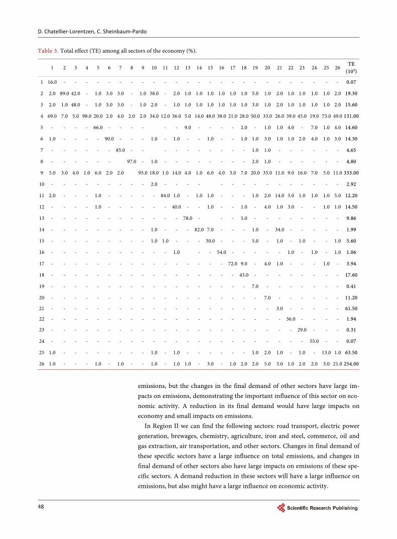
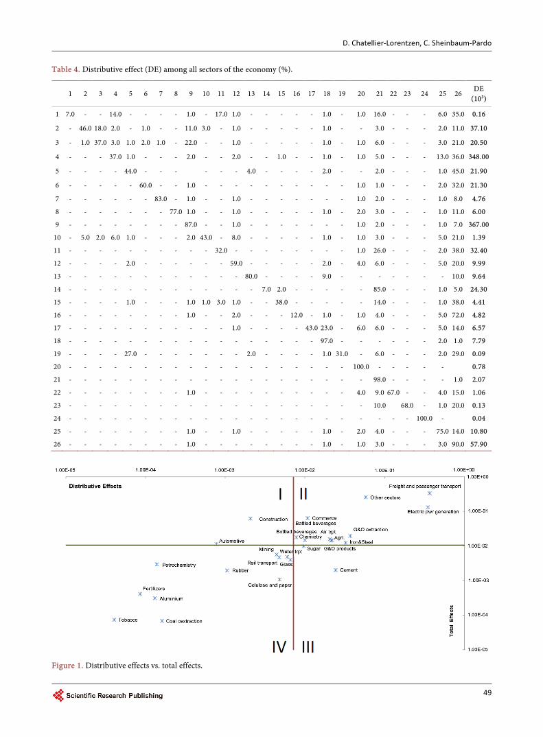
has on emissions levels. The Total Effect (TE) is the sum over i (columns of the matrix), and represents the change in emissions for all the economy due to a un-itary change in final demand of sector j. The Distributive Effect (DE) is the sum over j (rows of the matrix) and represents the change in emissions for all the economy due to a unitary change in each of the j sectors.

In addition, it is possible to separate each effect into two components [27]: Own Sector Effects (OE) that result from the changes in the final demand of each Own Sector (the diagonal elements of matrix ψ∆ ), and Structure Effects (SE) that result from the changes in other sectors of the economy.

2.3. Data Sources

The input-output model constructed in this work comes from a combination of two different databases available in Mexico, in addition to the IPCC emission factors [28]. These are the 2012 input-output matrixes provided by the National Institute of Statistics and Geography (INEGI) [29] with three different levels of sectorial disaggregation (i.e., 19 sectors, 70 subsectors, and 262 branches) and the 2012 National Energy Balance (NEB) [30] with a sectorial disaggregation of 17 producing sectors in addition to the agricultural sector, commercial sector, and transport sector, which subdivides itself into 4 sectors. In total, the NEB provides 26 different sectors. In order to match energy sectors from NEB and economy sectors from the input-output matrix, some sectors were summed up either in energy or I-O matrixes (Table 1). CO2, methane (CH4), and nitrous oxide (N2O) emissions are considered. The CO2-eq for CH4 and N2O, are 21 and 298 respectively.

2.4. Final Demand Projection for Year 2026

Final demand is projected to 2026 using Equation (13). The annual rate of growth was projected from 2003 to 2014 to 2026 (3.5% per year). Fuel structure, econo-my structure, and CO2-eq intensity are considered constant.

3. Results and Analysis

Table 2 presents CO2-eq emissions related to Mexican energy consumption and production in 2012 and estimations of a baseline scenario for 2026, as well as the variation in percentage. Changes in final demand carry a total emission increase of 3.4%.

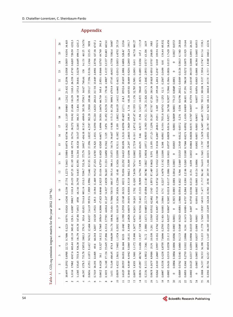
The total CO2-eq emissions impact matrix was calculated according to Equa-tion (10) and is presented in Table A1. Table 3 presents the TE, and Table 4 the DE, both for 2012. The diagonal elements of both of Table 3 and Table 4 are the percentages of OE in TE and DE, respectively. A large TE (final column of Table 3) means that the sector’s final demand has a high influence on total emissions, whereas a large DE (final column of Table 4) means that an overall change in final demand has a large influence on emissions from the specific sector. For example, a 1% increase in final demand of the coal mining sector would lead to a 0.07% increase of total CO2-eq emissions (Table 3, row 1, final column), whereas

D. Chatellier-Lorentzen, C. Sheinbaum-Pardo

46

Table 1. Sectors for input-output analysis: sector code.

Sector code Sector name

1 Coal mining

2 Gas and petroleum extraction

3 Petroleum processing and coking, gas production

4 Electric power generation

5 Agriculture: farming, forestry, animal, husbandry, and fishery

6 Air transport

7 Rail transport

8 Water transport

9 Freight and passenger road transport

10 Petro chemistry

11 Iron and steel basic products

12 Chemical fibers and resins, pharmaceutical products, paintings and adhesives, soaps and cleaners, plastic products, and other chemical products

13 Cane and beet sugar production, chocolates, and candies

14 Cement production and concrete products

15 Ferrous and non-ferrous mining, related mining services

16 Cellulose, paper, and cardboard manufacturing

17 Glass and glass products

18 Carbonated and noncarbonated sweet brewages, water purification, ice production, and beer and distillates manufacturing

19 Fertilizers, pesticides, and agrochemical

20 Car and truck manufacturing

21 Construction

22 Tire and rubber product manufacturing

23 Basic aluminum products

24 Tobacco product manufacturing

25 Wholesale, retail trade, hotels, restaurants

26 Other sectors

when there is a 1% increase of the final demand of all sectors, the emissions of coal mining would increase 0.16% with respect to the previous total emissions (Table 4, row 1, final column). The largest emissions come from the road trans-port sector. Therefore, a 1% increase in final demand of this sector would lead to a 333% increase of total CO2-eq emissions (Table 3, row 9, final column), and a 1% increase of the final demand of all sectors will represent an increase of 367% with respect to the previous total emissions (Table 4, row 9, final column).

Figure 1 presents the sectorial relation between DE vs. TE known as the Ras-mussen [31] classification discussed in [27] [31] that expresses the degree in which one industry output is used by other industries as an input. In this case, this grouping is based on the comparison of the median values of the sectorial DE and TE in a logarithmic scale. Table 5 shows the meaning of each region.

D. Chatellier-Lorentzen, C. Sheinbaum-Pardo

47

Table 2. Baseline scenario.

Sector code

Variation of final energy demand 2012-2016 (%)

Variation of emissions

2012-2026 (%)

Emissions 2012

(Tg CO2-eq)

Share of total

emissions

Emissions 2026

(Tg CO2-eq)

Position in Figure 1

1 −31.25% 0.00% 0.07 0.02% 0.07 VI

2 −2.00% 0.26% 15.18 3.71% 15.22 II

3 7.42% 0.31% 8.39 2.05% 8.41 II

4 −4.52% 6.41% 142.71 34.84% 151.85 II

5 11.40% 0.64% 8.97 2.19% 9.02 II

6 11.14% 0.51% 8.72 2.13% 8.76 II

7 0.00% 0.02% 1.95 0.48% 1.95 IV

8 12.01% 0.09% 2.46 0.60% 2.46 IV

9 3.36% 2.60% 150.38 36.71% 154.28 II

10 −1.31% 0.00% 0.06 0.01% 0.06 IV

11 35.99% 1.03% 13.28 3.24% 13.41 II

12 6.78% 0.16% 4.09 1.00% 4.1 II

13 1.29% 0.07% 3.95 0.96% 3.95 III

14 4.90% 0.07% 9.93 2.43% 9.94 III

15 8.14% 0.11% 1.81 0.44% 1.81 IV

16 18.88% 0.20% 1.98 0.48% 1.98 IV

17 4.71% 0.08% 2.69 0.66% 2.69 IV

18 4.50% 0.04% 3.19 0.78% 3.19 II

19 −4.92% 0.00% 0.04 0.01% 0.04 IV

20 13.48% 0.01% 0.32 0.08% 0.32 I

21 0.03% 0.00% 0.85 0.21% 0.85 I

22 9.14% 0.02% 0.43 0.11% 0.43 Iv

23 −14.47% 0.00% 0.05 0.01% 0.05 IV

24 −13.90% 0.00% 0.02 0.00% 0.02 IV

25 4.15% 0.12% 4.43 1.08% 4.43 II

26 52.58% 2.77% 23.73 5.79% 24.39 II

Total 3.43% 409.66 423.7 100.00% 423.68

A large discussion of Rasmussen method is developed in [27]. It corresponds

to a Classical Multiplier Method [32] [33]. Although there are new developments in the methods developed to analyze interlinkages among industrial sectors, this method is very useful in identifying total and distribution effects, particularly in the analysis of the economic impacts of GHG mitigation [34] [35] [36].

The sectors located in region I of Figure 1 are the construction and automo-tive sectors. These sectors use inputs of other productive processes, that is to say their consumption is influenced by the demand of other sectors. Consequently, mitigation policies that could affect the magnitude of their production might generate problems in their economic activity. In addition, changes in automotive industries’ (automotive production) final demand have a small influence on total

D. Chatellier-Lorentzen, C. Sheinbaum-Pardo

48

Table 3. Total effect (TE) among all sectors of the economy (%).

1 2 3 4 5 6 7 8 9 10 11 12 13 14 15 16 17 18 19 20 21 22 23 24 25 26

TE (103)

1 16.0 - - - - - - - - - - - - - - - - - - - - - - - - - 0.07

2 2.0 89.0 42.0 - 1.0 3.0 3.0 - 1.0 38.0 - 2.0 1.0 1.0 1.0 1.0 1.0 1.0 5.0 1.0 2.0 1.0 1.0 1.0 1.0 2.0 19.30

3 2.0 1.0 48.0 - 1.0 3.0 3.0 - 1.0 2.0 - 1.0 1.0 1.0 1.0 1.0 1.0 1.0 3.0 1.0 2.0 1.0 1.0 1.0 1.0 2.0 15.60

4 69.0 7.0 5.0 98.0 20.0 2.0 4.0 2.0 2.0 34.0 12.0 36.0 5.0 14.0 48.0 38.0 21.0 28.0 50.0 33.0 26.0 39.0 45.0 19.0 73.0 49.0 131.00

5 - - - - 66.0 - - - -

- - 9.0 - - - - 2.0 - 1.0 1.0 4.0 - 7.0 1.0 4.0 14.60

6 1.0 - - - - 90.0 - - - 1.0 - 1.0 - - 1.0 - - 1.0 1.0 3.0 1.0 1.0 2.0 4.0 1.0 3.0 14.30

7 - - - - - - 85.0 - -

- - - - - - - - 1.0 1.0 - - - - - - 4.65

8 - - - - - -

97.0 - 1.0 - - - - - - - - 2.0 1.0 - - - - - - 4.80

9 5.0 3.0 4.0 1.0 6.0 2.0 2.0

95.0 18.0 1.0 14.0 4.0 1.0 6.0 4.0 3.0 7.0 20.0 35.0 11.0 9.0 16.0 7.0 5.0 11.0 333.00

10 - - - - - - - - - 2.0 - - - -

- - - - - - - - - - - 2.92

11 2.0 - - - 1.0 - - - - - 84.0 1.0 - 1.0 1.0 - - - 1.0 2.0 14.0 3.0 1.0 1.0 1.0 5.0 12.20

12 - - - - 1.0 - - - - - - 40.0 - - 1.0 - - 1.0 - 4.0 1.0 3.0 - - 1.0 1.0 14.50

13 - - - - - - - - - - - - 78.0 -

- - 5.0 - - - - - - - - 9.86

14 - - - - - - - - - 1.0 - - - 82.0 7.0 - - - 1.0 - 34.0 - - - - - 1.99

15 - - - - - - - - - 1.0 1.0 - - - 30.0 - - - 5.0 - 1.0 - 1.0 - - 1.0 5.60

16 - - - - - - - - - - - 1.0

- - 54.0 - - - - - 1.0 - 1.0 - 1.0 1.06

17 - - - - - - - - - - - - - - - - 72.0 9.0 - 4.0 1.0 - - - 1.0 - 3.94

18 - - - - - - - - - - - - - - - - - 43.0 - - - - - - - - 17.60

19 - - - - - - - - - - - - - - - - - - 7.0 - - - - - - - 0.41

20 - - - - - - - - - - - - - - - - - - - 7.0 - - - - - - 11.20

21 - - - - - - - - - - - - - - - - - - - - 3.0 - - - - - 61.50

22 - - - - - - - - - - - - - - - - - - - - - 36.0 - - - - 1.94

23 - - - - - - - - - - - - - - - - - - - - - - 29.0 - - - 0.31

24 - - - - - - - - - - - - - - - - - - - - - - - 55.0 - - 0.07

25 1.0 - - - - - - - - 1.0 - 1.0 - - - - - - 1.0 2.0 1.0 - 1.0 - 13.0 1.0 63.50

26 1.0 - - - 1.0 - 1.0 - - 1.0 - 1.0 1.0 - 3.0 - 1.0 2.0 2.0 5.0 3.0 1.0 2.0 2.0 3.0 21.0 254.00

emissions, but the changes in the final demand of other sectors have large im-pacts on emissions, demonstrating the important influence of this sector on eco- nomic activity. A reduction in its final demand would have large impacts on economy and small impacts on emissions.

In Region II we can find the following sectors: road transport, electric power generation, brewages, chemistry, agriculture, iron and steel, commerce, oil and gas extraction, air transportation, and other sectors. Changes in final demand of these specific sectors have a large influence on total emissions, and changes in final demand of other sectors also have large impacts on emissions of these spe-cific sectors. A demand reduction in these sectors will have a large influence on emissions, but also might have a large influence on economic activity.

D. Chatellier-Lorentzen, C. Sheinbaum-Pardo

49

Table 4. Distributive effect (DE) among all sectors of the economy (%).

1 2 3 4 5 6 7 8 9 10 11 12 13 14 15 16 17 18 19 20 21 22 23 24 25 26

DE (103)

1 7.0 - - 14.0 - - - - 1.0 - 17.0 1.0 - - - - - 1.0 - 1.0 16.0 - - - 6.0 35.0 0.16

2 - 46.0 18.0 2.0 - 1.0 - - 11.0 3.0 - 1.0 - - - - - 1.0 - - 3.0 - - - 2.0 11.0 37.10

3 - 1.0 37.0 3.0 1.0 2.0 1.0 - 22.0 - - 1.0 - - - - - 1.0 - 1.0 6.0 - - - 3.0 21.0 20.50

4 - - - 37.0 1.0 - - - 2.0 - - 2.0 - - 1.0 - - 1.0 - 1.0 5.0 - - - 13.0 36.0 348.00

5 - - - - 44.0 - - -

- - - 4.0 - - - - 2.0 - - 2.0 - - - 1.0 45.0 21.90

6 - - - - - 60.0 - - 1.0 - - - - - - - - - - 1.0 1.0 - - - 2.0 32.0 21.30

7 - - - - - - 83.0 - 1.0 - - 1.0 - - - - - - - 1.0 2.0 - - - 1.0 8.0 4.76

8 - - - - - - - 77.0 1.0 - - 1.0 - - - - - 1.0 - 2.0 3.0 - - - 1.0 11.0 6.00

9 - - - - - - - - 87.0 - - 1.0 - - - - - - - 1.0 2.0 - - - 1.0 7.0 367.00

10 - 5.0 2.0 6.0 1.0 - - - 2.0 43.0 - 8.0 - - - - - 1.0 - 1.0 3.0 - - - 5.0 21.0 1.39

11 - - - - - - - - - - 32.0 - - - - - - - - 1.0 26.0 - - - 2.0 38.0 32.40

12 - - - - 2.0 - - - - - - 59.0 - - - - - 2.0 - 4.0 6.0 - - - 5.0 20.0 9.99

13 - - - - - - - - - - - - 80.0 - - - - 9.0 - - - - - - - 10.0 9.64

14 - - - - - - - - - - - - - 7.0 2.0 - - - - - 85.0 - - - 1.0 5.0 24.30

15 - - - - 1.0 - - - 1.0 1.0 3.0 1.0 - - 38.0 - - - - - 14.0 - - - 1.0 38.0 4.41

16 - - - - - - - - 1.0 - - 2.0 - - - 12.0 - 1.0 - 1.0 4.0 - - - 5.0 72.0 4.82

17 - - - - - - - - - - - 1.0 - - - - 43.0 23.0 - 6.0 6.0 - - - 5.0 14.0 6.57

18 - - - - - - - - - - - - - - - - - 97.0 - - - - - - 2.0 1.0 7.79

19 - - - - 27.0 - - - - - - - 2.0 - - - - 1.0 31.0 - 6.0 - - - 2.0 29.0 0.09

20 - - - - - - - - - - - - - - - - - - - 100.0 - - - - -

0.78

21 - - - - - - - - - - - - - - - - - - - - 98.0 - - - - 1.0 2.07

22 - - - - - - - - 1.0 - - - - - - - - - - 4.0 9.0 67.0 - - 4.0 15.0 1.06

23 - - - - - - - - - - - - - - - - - - - - 10.0

68.0 - 1.0 20.0 0.13

24 - - - - - - - - - - - - - - - - - - - - - - - 100.0 -

0.04

25 - - - - - - - - 1.0 - - 1.0 - - - - - 1.0 - 2.0 4.0 - - - 75.0 14.0 10.80

26 - - - - - - - - 1.0 - - - - - - - - 1.0 - 1.0 3.0 - - - 3.0 90.0 57.90

Figure 1. Distributive effects vs. total effects.

D. Chatellier-Lorentzen, C. Sheinbaum-Pardo

50

Table 5. Regions in Figure 1.

Regions Distributive Effects Total Effects

I Small changes in final demand of the specific sector have a small influence on total emissions

Large changes in final demand of other sectors have large impacts on emissions of the specific sector

II Large changes in final demand of the specific sector have a large influence on total emissions

Large changes in final demand of other sectors have large impacts on emissions of the specific sector

III Large changes in final demand of the specific sector have a large influence on total emissions

Small changes in final demand of other sectors have small impacts on emissions of the specific sector

IV Small changes in final demand of the specific sector have a small influence on total emissions

Small changes in final demand of other sectors have small impacts on emissions of the specific sector

The sugar industry and the cement industry are the sectors in Region III.

Changes in final demand of these specific sectors have a large influence on total emissions, but changes in final demand of other sectors have small impacts on emissions of these specific sectors. In Region IV are less relevant sectors in terms of final demand and emissions. A reduction in CO2-eq emissions of these sectors will not have an important impact on overall emissions, because the share in the distribution of emissions is low.

Another important observation from Figure 1 is how construction and ce-ment (in region III) are linked. It is possible to connect a line with both sectors that crosses the mean values (the center of the graphic). TE of the construction sector that affects the cement sector is the same amount as the DE of the cement sector received from the construction sector. Hence, if the final demand of sector 21 decreases, the emissions from sector 14 will also decrease. This relation also means that if the cement for construction is substituted with other materials, emissions from sector 14 will decrease.

5. Concluding Remarks

In this paper, an input-output methodology is developed to analyze energy-re- lated GHG emissions of the Mexican economy. The paper also analyzes total and distributive effects that final demand has on emissions levels. It also identifies Own Sector Effects (OE) that result from the changes in the final demand of each Own Sector (the diagonal elements of matrix ψ∆ ), and Structure Effects (SE) that result from the changes in other sectors of the economy.

According to IPCC’s fifth assessment report [37], the main mitigation strate-gies for the industrial sector are 1) reduction of emission intensity expressed as the ratio of GHG emissions to energy use; 2) reduction of energy intensity, measured as unit energy consumption in physical units (or in this case monetary units); 3) increase in material efficiency, which is the amount of material re-quired to produce one product; and 4) reduction of product service intensity, which is the level of service provided by a product.

D. Chatellier-Lorentzen, C. Sheinbaum-Pardo

51

These strategies can be applied to sectors that appear in Region II and III to obtain the largest reduction in GHG emissions. Strategies 3) and 4) are related to a reduction in material or product production and will have an important effect on the economy, particularly in those sectors that appear in Region II. The alignment of strategies to fulfill the goals of the NDC requires additional analy-sis. Additional work is necessary to evaluate policies. The results presented in this paper are a useful tool for a GEM for the Mexican economy.

References [1] Rogelj, J., den Elzen, M., Höhne, N., Fransen, T., Fekete, H., Winkler, H., Schaeffer,

R.,Sha, F., Riahi, K. and Meinshausen, M. (2016) Paris Agreement Climate Propos-als Need a Boost to Keep Warming Well Below 2˚C. Nature, 534, 631-639. https://doi.org/10.1038/nature18307

[2] COP21 Country by Country. http://www.cop21.gouv.fr/en/learn/country-by-country/

[3] LEY General de Cambio Climático. http://www.diputados.gob.mx/LeyesBiblio/ref/lgcc.htm

[4] Markandya, A., Halsnaes, K., Lanza, A., Matsuoka, Y., Maya S., Pan J., Shogren, J., Seroa de Motta, R. and Zhang, T. (2001) Mitigation. In: Metz, B., Davidson, O., Swart, R. and Pan, J., Eds., Contribution of Working Group III to the Third As-sessment Report of the Intergovernmental Panel on Climate Change, Cambridge University Press, UK.

[5] Leontief, W.W. (1936) Quantitative Input and Output Relations in the Economic Systems of the United States. The Review of Economics and Statistics, 18, 105-125. https://doi.org/10.2307/1927837

[6] Lenzen, M.A. (2001) Generalized Input-Output Multiplier Calculus for Australia. Economic Systems Research, 13, 65-92. https://doi.org/10.1080/09535310120026256

[7] Alcántara, V. and Padilla, E. (2009) Input-Output Subsystems and Pollution: An Application to the Service Sector and CO2 Emissions in Spain. Ecological Econom-ics, 68, 905-914. https://doi.org/10.1016/j.ecolecon.2008.07.010

[8] Proops, J.L.R., Faber, M. and Wagenhals, G. (2012) Reducing CO2 Emissions: A Comparative Input-Output-Study for Germany and the UK. Springer-Verlag, Berlin Heidelberg, 304-314.

[9] Tarancón, M.A., del Río, P. and Callejas Albiñana, F. (2019) Assessing the Influence of Manufacturing Sectors on Electricity Demand. A Cross-Country Input-Output Approach. Energy Policy, 38, 1900-1908. https://doi.org/10.1016/j.enpol.2009.11.070

[10] Tarancón, M.A. and Del Río, P. (2012) Assessing Energy-Related CO2 Emissions with Sensitivity Analysis and Input-Output Techniques. Energy, 37, 161-170. https://doi.org/10.1016/j.energy.2011.07.026

[11] Alcántara, V., Tarancón, M.A. and del Río, P. (2013) Assessing the Technological Responsibility of Productive Structures in Electricity Consumption. Energy Eco-nomics, 40, 457-467. https://doi.org/10.1016/j.eneco.2013.07.012

[12] Chen, G.Q., Guo, S., Shao, L., Li, J.S. and Chen, Z.M. (2013) Three-Scale In-put-Output Modeling for Urban Economy: Carbon Emission by Beijing 2007. Com-munications in Nonlinear Science and Numerical Simulation, 18, 2493-2506. https://doi.org/10.1016/j.cnsns.2012.12.029

[13] Cui, L.B., Peng, P. and Zhu, L. (2015) Embodied Energy, Export Policy Adjustment

D. Chatellier-Lorentzen, C. Sheinbaum-Pardo

52

and China’s Sustainable Development: A Multi-Regional Input-Output Analysis. Energy, 82, 457-467. https://doi.org/10.1016/j.energy.2015.01.056

[14] Lin, B. and Xie, X. (2016) CO2 Emissions of China’s Food Industry: An Input- Output Approach. Journal of Cleaner Production, 112, 1410-1421. https://doi.org/10.1016/j.jclepro.2015.06.119

[15] Chen, G., Hadjikakou, M. and Wiedmann, T. (2016) Urban Carbon Transforma-tions: Unravelling Spatial and Inter-Sectoral Linkages for Key City Industries Based on Multi-Region Input-Output Analysis. Journal of Cleaner Production. https://doi.org/10.1016/j.jclepro.2016.04.046

[16] Li, Z., Pan, L., Fu, F., Liu, P., Ma, L. and Amorelli, A. (2014) China’s Regional Dis-parities in Energy Consumption: An Input-Output Analysis. Energy, 78, 426-438. https://doi.org/10.1016/j.energy.2014.10.030

[17] Wiebe, K.S., Bruckner, M., Giljum, S. and Lutz, C. (2012) Calculating Energy- Related CO2 Emissions Embodied in International Trade Using a Global Input- Output Model. Economic Systems Research, 24,113-139. https://doi.org/10.1080/09535314.2011.643293

[18] Su, B. and Ang, B.W. (2013) Input-Output Analysis of CO2 Emissions Embodied in Trade: Competitive versus Non-Competitive Imports. Energy Policy, 56, 83-87. https://doi.org/10.1016/j.enpol.2013.01.041

[19] Cortés-Borda, D., Guillén-Gosálbez, G. and Jiménez, L. (2015) Assessment of Nuc-lear Energy Embodied in International Trade Following a World Multi-Regional Input-Output Approach. Energy, 91, 91-101. https://doi.org/10.1016/j.energy.2015.07.117

[20] Nordhaus, W.D. and Yang, Z. (1996) A Regional Dynamic General-Equilibrium Model of Alternative Climate-Change Strategies. American Economic Review, 86, 741-765.

[21] Rose, A. (1995) Input-Output Economics and Computable General Equilibrium Models. Structural Change and Economic Dynamics, 6, 295-304. https://doi.org/10.1016/0954-349X(95)00018-I

[22] Bauer, N., Mouratiadou, I., Luderer, G., Baumstark, L., Brecha, R.J., Edenhofer, O., et al. (2013) Global Fossil Energy Markets and Climate Change Mitigation—An Analysis with REMIND. Climate Change, 136, 69-82. https://doi.org/10.1007/s10584-013-0901-6

[23] Sue Wing, I.N.J. and Timilsina, G.R. (2016) Technology Strategies for Low-Carbon Economic Growth: A General Equilibrium Assessment. Report No. 7742, The World Bank, Washington DC. http://econpapers.repec.org/paper/wbkwbrwps/7742.htm

[24] Böhringer, C., Carbone, J.C. and Rutherford, T.F. (2016) The Strategic Value of Carbon Tariffs. American Economic Journal: Economic Policy, 8, 28-51. https://doi.org/10.1257/pol.20130327

[25] IV LRG (1995) Trade Liberalization and Pollution: An Input-Output Study of Car-bon Dioxide Emissions in Mexico. Economic Systems Research, 7, 309-320. https://doi.org/10.1080/09535319500000026

[26] Wiedmann, T., Lenzen, M., Turner, K. and Barrett, J. (2007) Examining the Global Environmental Impact of Regional Consumption Activities—Part 2: Review of In-put-Output Models for the Assessment of Environmental Impacts Embodied in Trade. Ecological Economics, 61, 15-26. https://doi.org/10.1016/j.ecolecon.2006.12.003

[27] Alcántara, V. and Padilla E. (2003) “Key” Sectors in Final Energy Consumption: An Input-Output Application to the Spanish Case. Energy Policy, 31, 1673-1678.

D. Chatellier-Lorentzen, C. Sheinbaum-Pardo

53

https://doi.org/10.1016/S0301-4215(02)00233-1

[28] IPCC (2006) Task Force on National Greenhouse Gas Inventories. http://www.ipcc-nggip.iges.or.jp/public/2006gl/

[29] Instituto Nacional de Estadística y Geografía. Input-Output Matrixes. http://www3.inegi.org.mx/sistemas/biblioteca/ficha.aspx?upc=702825003429

[30] SENER Sistema de Información Energética. http://sie.energia.gob.mx/

[31] Rasmussen, P.N. (1956) Studies in Inter-Sectoral Relations. Einar Harcks, Køben-havn.

[32] Wang, Y., Wang, W., Mao, G., Cai, H., Zuo, J., Wang, L. and Zhao, P. (2013) Indus-trial CO2 Emissions in China Based on the Hypothetical Extraction Method: Lin-kage Analysis. Energy Policy, 62, 1238-1244. https://doi.org/10.1016/j.enpol.2013.06.045

[33] Harada, T. (2015) Changing Productive Relations, Linkage Effects, and Industriali-zation. Economic Systems Research, 27, 374-390. https://doi.org/10.1080/09535314.2015.1081876

[34] Piaggio, M., Alcántara, V. and Padilla, E. (2014) Greenhouse Gas Emissions and Economic Structure in Uruguay. Economic Systems Research, 26, 155-176. https://doi.org/10.1080/09535314.2013.869559

[35] Chang, N. and Lahr, M.L. (2016) Changes in China’s Production-Source CO2 Emis-sions: Insights from Structural Decomposition Analysis and Linkage Analysis. Eco-nomic Systems Research, 28, 224-242. https://doi.org/10.1080/09535314.2016.1172476

[36] Lamonica, G.R. and Mattioli, E. (2015) Research Note: The Impact of the Tourism Industry on the World’s Largest Economies—An Input-Output Analysis. Tourism Economics, 21, 419-426. https://doi.org/10.5367/te.2013.0363

[37] Fischedick, M., Roy, J., Abdel-Aziz, A., Acquaye, A., Allwood, J.M., Ceron, J.-P., Geng, Y., Kheshgi, H., Lanza, A., Perczyk, D., Price, L., Santalla, E., Sheinbaum, C. and Tanaka, K. (2014) Industry. In: Edenhofer, O., Pichs-Madruga, R., Sokona, Y., Farahani, E., Kadner, S., Seyboth, K., Adler, A., Baum, I., Brunner, S., Eickemeier, P., Kriemann, B., Savolainen, J., Schlömer, S., von Stechow, C., Zwickel, T. and Minx, J.C., Eds., Climate Change 2014: Mitigation of Climate Change, Contribution of Working Group III to the Fifth Assessment Report of the Intergovernmental Panel on Climate Change, Cambridge University Press, Cambridge and New York, 739-810. http://www.ipcc.ch/report/ar5/wg3/

D. Chatellier-Lorentzen, C. Sheinbaum-Pardo

54

Appendix

Submit or recommend next manuscript to SCIRP and we will provide best service for you:

Accepting pre-submission inquiries through Email, Facebook, LinkedIn, Twitter, etc. A wide selection of journals (inclusive of 9 subjects, more than 200 journals) Providing 24-hour high-quality service User-friendly online submission system Fair and swift peer-review system Efficient typesetting and proofreading procedure Display of the result of downloads and visits, as well as the number of cited articles Maximum dissemination of your research work

Submit your manuscript at: http://papersubmission.scirp.org/ Or contact epe@scirp.org