Assessing the Effects of Cattle Exclusion Practices on ... · Figure 3.5 Automatic sampler (ISCO...

Assessing the Effects of Cattle Exclusion Practices on Water Quality

in Headwater Streams in the Shenandoah Valley, Virginia

Nancy Jane Maschke

Thesis submitted to the faculty of the Virginia Polytechnic Institute and State University in

partial fulfillment of the requirements for the degree of

Master of Science

In

Biological Systems Engineering

Conrad D. Heatwole

Brian L. Benham

Darrell J. Bosch

Gene R. Yagow

27 January 2012

Blacksburg, VA

Keywords: cattle exclusion, flash grazing, water quality, BMP

Assessing the Effects of Cattle Exclusion Practices on Water Quality in Headwater Streams in

the Shenandoah Valley, Virginia

Nancy Maschke

ABSTRACT

Livestock best management practices (BMPs) such as streamside exclusion fencing are installed

to reduce cattle impacts on stream water quality such as increases in bacteria through direct

deposition and sediment through trampling. The main objective of this study is to assess the

effects of different cattle management strategies on water quality.

The project site was located near Keezletown, VA encompassing Cub Run and Mountain Valley

Road Tributary streams. During two, one-week studies, eight automatic water samplers took

two-hour composites for three periods: baseline, cattle access, and recovery. During the cattle

access period, livestock were able to enter the riparian zone normally fenced off. Water samples

were analyzed for E.coli, sediment, and nutrients to understand the short-term, high-density, or

flash grazing, impact on water quality. Additional weekly grab and storm samples were

collected.

Results show that cattle do not have significant influence on pollutant concentrations except in

stream locations where cattle gathered for an extensive period of time. Approximately three

cattle in the stream created an increase in turbidity above baseline concentrations. E.coli and

TSS concentrations of the impacted sites returned to baseline within approximately 6 to 20 hours

of peak concentrations. Weekly samples show that flash grazing does not have a significant

influence on pollutant concentrations over a two-year time frame. Sediment loads from storms

and a flash grazing event showed similar patterns. Pollutant concentrations through the

permanent exclusion fencing reach tended to decrease for weekly and flash grazing samples.

iii

Acknowledgements

I would first like to thank the members of my committee for their help and guidance through my

research: Dr. Brian Benham, Dr. Gene Yagow, and Dr. Darrell Bosch. I especially would like to

thank my advisor, Dr. Conrad Heatwole, for giving me this opportunity as well as for his effort,

time, and support during my graduate career with research and classes.

A big thank you goes all those that helped me prepare, collect, and analyze samples: Sarah

(Sally) Walker, Kendall Price, Aaron Estep, Lucas Blosser, Amanda Graumann, and others.

Without your help, this project would not have run as smoothly as it did.

This project would not be possible if it were not for the farmers and land owners that allowed me

to sample on their property. I appreciate the time out of their schedules to open gates and move

cattle around to accommodate my research needs.

A final thank you goes to John Spicher and Eastern Mennonite University in Harrisonburg,

Virginia for very generously providing us space and access to their labs to analyze samples.

This research is one component of the project “Adaptive and community-based strategies to

reduce nutrient loads.” (Project #2007-08-003) funded through the National Fish and Wildlife

Foundation’s 2007 Chesapeake Bay Targeted Watershed Grants Program.

iv

Table of Contents

List of Figures................................................................................................................................. vii

List of Tables ....................................................................................................................................x

1 Introduction ................................................................................................................................. 1

2 Literature Review ........................................................................................................................ 3

2.1 Best Management Practices ................................................................................................. 3

2.2 Buffers ................................................................................................................................... 3

2.3 Animal Stocking Density ....................................................................................................... 4

2.4 Pasture Characteristics ......................................................................................................... 5

2.5 Alternative Water ................................................................................................................... 5

2.6 Specified Entrance Points ..................................................................................................... 6

2.7 Cattle Impacts on the Stream Environment .......................................................................... 7

2.7.1 Stream Bed and Bank Impacts ...................................................................................... 7

2.7.2 Nutrients ......................................................................................................................... 9

2.7.3 Bacteria ......................................................................................................................... 11

2.7.4 pH and Salinity ............................................................................................................. 13

2.7.5 Benthic Macroinvertebrates ......................................................................................... 13

2.8 Flash Grazing ...................................................................................................................... 14

2.9 Alternatives to Fencing ....................................................................................................... 15

2.9.1 Animal Behavior ........................................................................................................... 16

2.9.2 Cattle Management ...................................................................................................... 16

2.9.3 Virtual Fencing .............................................................................................................. 17

2.10 Stakeholders ..................................................................................................................... 17

2.10.1 Cattle Exclusion Economics ....................................................................................... 18

2.11 Summary ........................................................................................................................... 18

3 Methods .................................................................................................................................... 19

3.1 Site Descriptions ................................................................................................................. 19

v

3.2 Sampling ............................................................................................................................. 21

3.2.1 Flash Grazing Sampling ............................................................................................... 21

3.2.2 Cattle ............................................................................................................................ 23

3.2.3 Determining Baseflow Conditions ................................................................................ 23

3.2.4 Weekly Sampling .......................................................................................................... 24

3.2.5 Storm Sampling ............................................................................................................ 24

3.2.6 Quality Control/Quality Assurance ............................................................................... 24

3.3 Sample Analysis .................................................................................................................. 25

3.3.1 pH/Electrical Conductivity (EC) .................................................................................... 25

3.3.2 Turbidity ........................................................................................................................ 25

3.3.3 Total Suspended Solids (TSS) ..................................................................................... 25

3.3.4 E. Coli Bacteria ............................................................................................................. 26

3.3.5 Nutrients ....................................................................................................................... 26

3.4 Salt Tracer ........................................................................................................................... 26

3.5 Cameras .............................................................................................................................. 27

3.5.1 Determining Livestock Densities .................................................................................. 28

3.6 Summary ............................................................................................................................. 29

4 Results ...................................................................................................................................... 31

4.1 Weather Data ...................................................................................................................... 31

4.1.1 Study 1 .......................................................................................................................... 31

4.1.2 Study 2 .......................................................................................................................... 33

4.2 Flow ..................................................................................................................................... 36

4.3 Cattle Density and Pollutant Concentrations ...................................................................... 39

4.4 Statistical Analysis .............................................................................................................. 45

4.4.1 Study 1 .......................................................................................................................... 45

4.4.2 Study 2 .......................................................................................................................... 46

4.4.3 Weekly Samples ........................................................................................................... 46

vi

4.5 Study 1 ................................................................................................................................ 47

4.5.1 Time Series Data .......................................................................................................... 47

4.5.2 Statistical Analysis ........................................................................................................ 50

4.6 Study 2 ................................................................................................................................ 55

4.6.1 Time Series Data .......................................................................................................... 55

4.6.2 Statistical Analysis ........................................................................................................ 59

4.7 Return to Baseline Concentrations ..................................................................................... 63

4.8 Turbidity as an Indicator of Impact...................................................................................... 66

4.9 Storm Concentrations ......................................................................................................... 72

4.10 Weekly Grab Samples ...................................................................................................... 74

4.11 Effects of CREP Zone ....................................................................................................... 78

5 Discussion and Conclusions ..................................................................................................... 81

6 Limitations and Recommendations .......................................................................................... 84

7 References ................................................................................................................................ 86

Appendix A. Stage-Discharge Curves .......................................................................................... 91

Appendix B. R Statistical Code ..................................................................................................... 94

Appendix C. Statistical Means and Confidence Intervals .......................................................... 101

Appendix D. Storm TSS Time Series and Hydrographs ............................................................ 107

Appendix E. Comparing Manual and ISCO Samples ................................................................ 109

Appendix F. QA/QC .................................................................................................................... 114

Appendix G. Salt Tracer Results ................................................................................................ 117

Appendix H. Cattle Densities by Zone ........................................................................................ 118

Appendix I. pH and EC Boxplots for Studies 1 and 2 ................................................................ 124

Appendix J. pH, EC, NO3-N, and TN Boxplots for Weekly Grab Samples ................................ 126

vii

List of Figures

Figure 3.1 Project site pasture area, riparian zone for flash grazing, and CREP fencing zone

located in Rockingham County, Virginia. (Source: Google Earth) .............................. 19

Figure 3.2 Mountain Valley Road Tributary looking downstream (Source: Nancy Maschke) .... 20

Figure 3.3 Cub Run looking downstream (Source: Nancy Maschke) ......................................... 21

Figure 3.4 Schematic of study site showing sampling locations ................................................. 22

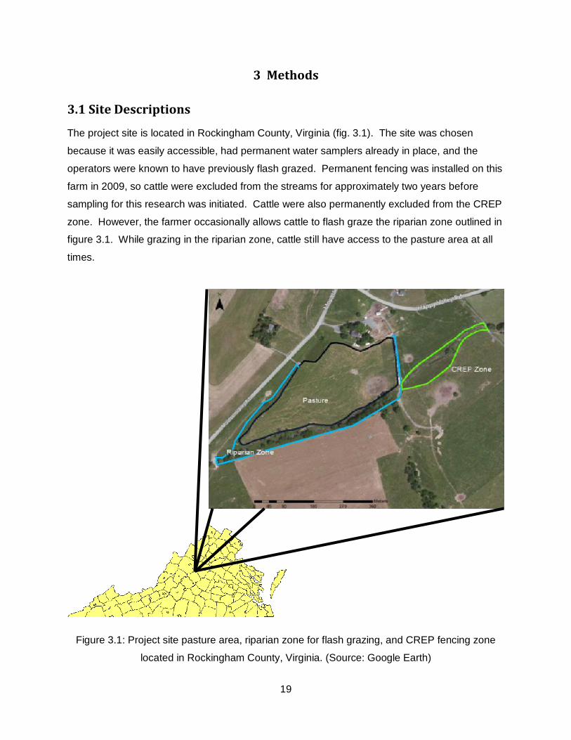
Figure 3.5 Automatic sampler (ISCO 6712) with 24 1-L bottles. (Source: Nancy Maschke) ..... 23

Figure 3.6 Camera areas and zones (Source: Google Earth) .................................................... 28

Figure 4.1 July rainfall from the HOBO weather station at Mountain Valley Road .................... 31

Figure 4.2 July rainfall from KVAMCGAH2 station in McGaheysville, VA found through Weather

Underground ................................................................................................................ 32

Figure 4.3 Temperature data, Study 1 ........................................................................................ 32

Figure 4.4 Solar radiation data, Study 1 ...................................................................................... 33

Figure 4.5 Relative humidity data, Study 1 ................................................................................. 33

Figure 4.6 August rainfall from the HOBO station at Mountain Valley Road .............................. 34

Figure 4.7 August rainfall from KVAMCGAH2 station in McGaheysville, VA found through

Weather Underground ................................................................................................. 34

Figure 4.8 Temperature data, Study 2 ........................................................................................ 35

Figure 4.9 Solar radiation data, Study 2 ...................................................................................... 35

Figure 4.10 Relative humidity data, Study 2 ............................................................................... 36

Figure 4.11 Flow by site and date ............................................................................................... 37

Figure 4.12 Bacteria (E. coli) count time series for Cub Run stations (box indicates period 2),

Study 1 ......................................................................................................................... 48

Figure 4.13 Bacteria (E. coli) count time series for CM, CR3, and MV2 (box indicates period 2),

Study 1 ......................................................................................................................... 48

Figure 4.14 TSS time series for Cub Run sites (box indicates period 2), Study 1 ..................... 49

Figure 4.15 TSS time series for CR3, CM, and MV2 (box indicates period 2), Study 1 ............ 49

Figure 4.16 Bacteria (E. coli) count time series for Cub Run (box indicates period 2), Study 2..

...................................................................................................................................... 56

Figure 4.17 Bacteria (E. coli) count time series for CM, CR3, and MV2 (box indicates period 2),

Study 2 ......................................................................................................................... 56

Figure 4.18 Bacteria (E. coli) count time series for Mountain Valley Road Tributary (box

indicates period 2), Study 2 ......................................................................................... 57

Figure 4.19 TSS time series for Cub Run (box indicates period 2), Study 2 .............................. 57

viii

Figure 4.20 TSS time series for CM, CR3, and MV2 (box indicates period 2), Study 2 ............ 58

Figure 4.21 TSS time series for Mountain Valley Road Tributary (box indicates period 2), Study

2 .................................................................................................................................... 58

Figure 4.22 Turbidity time series for Cub Run (box indicates period 2), Study 1 ....................... 68

Figure 4.23 Turbidity time series for CM, CR3, and MV2 (box indicates period 2), Study 1 ..... 68

Figure 4.24 Turbidity time series for CM, CR3, and MV2 (box indicates period 2), Study 2 ..... 69

Figure 4.25 Turbidity time series for MV (box indicates period 2), Study 2 ................................. 69

Figure 4.26 Zone 2 turbidity and maximum number of cattle in fencing, Study 1 ...................... 70

Figure 4.27 Zone 3 turbidity and average number of cattle in stream, Study 1 ......................... 70

Figure 4.28 Zone 3 turbidity and average number of cattle in fencing, Study 2 ......................... 71

Figure 4.29 Zone 4 turbidity and maximum number of cattle in stream, Study 2 ....................... 71

Figure A.1 CR1 2011 stage-discharge curve .............................................................................. 91

Figure A.2 CR3 2011 stage-discharge curve ............................................................................... 91

Figure A.3 MV1 2011 stage-discharge curve .............................................................................. 92

Figure A.4 MV2 2011 stage-discharge curve .............................................................................. 92

Figure A.5 2010 stage-discharge curves for CR1, CR3, MV1, and MV2 ................................... 93

Figure D.1 Storm III TSS and flow for MV2 ............................................................................... 107

Figure D.2 Storm V TSS and flow for MV2 ............................................................................... 107

Figure D.3 Storm IX TSS and flow for MV2 .............................................................................. 108

Figure D.4 Storm X TSS and flow for MV2 ............................................................................... 108

Figure E.1 Total suspended solids (TSS) for manual and ISCO grab samples by site ........... 109

Figure E.2 E. coli bacteria for manual and ISCO grab samples by site ................................... 109

Figure E.3 pH for manual and ISCO grab samples by site ....................................................... 110

Figure E.4 Electrical conductivity (EC) for manual and ISCO grab samples by site ................ 111

Figure E.5 Turbidity for manual and ISCO grab samples by site ............................................. 111

Figure E.6 Bacteria (E. coli) boxplot for manual and ISCO samples ........................................ 112

Figure E.7 Bacteria (E. coli) plot of manual versus ISCO samples .......................................... 112

Figure E.8 TSS boxplot for manual and ISCO samples ........................................................... 113

Figure E.9 TSS for manual versus ISCO samples and 1:1 line ................................................ 113

Figure F.1 E. coli bacteria for DI blanks by site......................................................................... 114

Figure F.2 pH for DI banks by site ............................................................................................. 114

Figure F.3 Electrical conductivity (EC) for DI blanks by site ..................................................... 115

Figure F.4 Turbidity for DI blanks by site................................................................................... 115

Figure I.1 pH by site, Study 1 .................................................................................................... 124

ix

Figure I.2 Electrical conductivity (EC) by site, Study 1 ............................................................. 124

Figure I.3 pH boxplot by site, Study 2 ....................................................................................... 125

Figure I.4 Electrical conductivity (EC) boxplot by site, Study 2 ................................................ 125

Figure I.5 Boxplots of pH for the weekly grab samples by site and year .................................. 126

Figure I.6 Boxplots of electrical conductivity for the weekly grab samples by site and year .... 126

Figure I.7 Boxplots of total nitrogen for weekly grab samples by site and year ....................... 127

Figure I.8 Boxplots of NO3-N for weekly grab samples by site and year .................................. 127

x

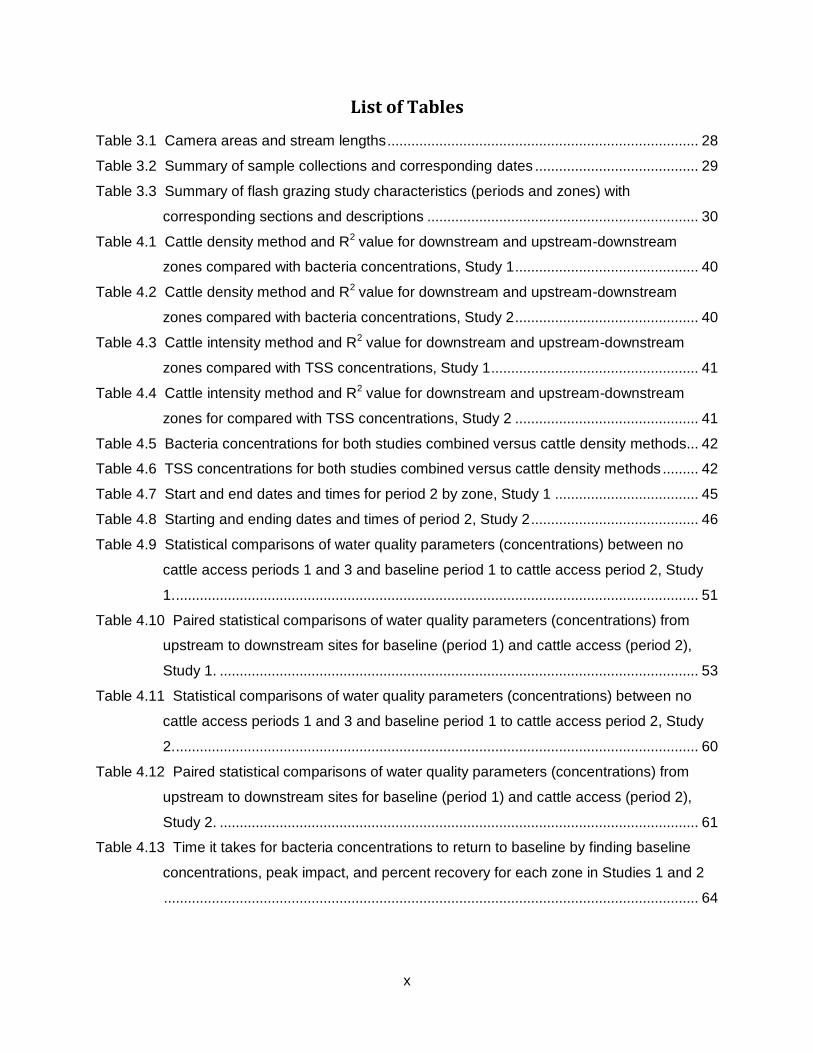
List of Tables

Table 3.1 Camera areas and stream lengths .............................................................................. 28

Table 3.2 Summary of sample collections and corresponding dates ......................................... 29

Table 3.3 Summary of flash grazing study characteristics (periods and zones) with

corresponding sections and descriptions .................................................................... 30

Table 4.1 Cattle density method and R2 value for downstream and upstream-downstream

zones compared with bacteria concentrations, Study 1 .............................................. 40

Table 4.2 Cattle density method and R2 value for downstream and upstream-downstream

zones compared with bacteria concentrations, Study 2 .............................................. 40

Table 4.3 Cattle intensity method and R2 value for downstream and upstream-downstream

zones compared with TSS concentrations, Study 1 .................................................... 41

Table 4.4 Cattle intensity method and R2 value for downstream and upstream-downstream

zones for compared with TSS concentrations, Study 2 .............................................. 41

Table 4.5 Bacteria concentrations for both studies combined versus cattle density methods... 42

Table 4.6 TSS concentrations for both studies combined versus cattle density methods ......... 42

Table 4.7 Start and end dates and times for period 2 by zone, Study 1 .................................... 45

Table 4.8 Starting and ending dates and times of period 2, Study 2 .......................................... 46

Table 4.9 Statistical comparisons of water quality parameters (concentrations) between no

cattle access periods 1 and 3 and baseline period 1 to cattle access period 2, Study

1. ................................................................................................................................... 51

Table 4.10 Paired statistical comparisons of water quality parameters (concentrations) from

upstream to downstream sites for baseline (period 1) and cattle access (period 2),

Study 1. ........................................................................................................................ 53

Table 4.11 Statistical comparisons of water quality parameters (concentrations) between no

cattle access periods 1 and 3 and baseline period 1 to cattle access period 2, Study

2. ................................................................................................................................... 60

Table 4.12 Paired statistical comparisons of water quality parameters (concentrations) from

upstream to downstream sites for baseline (period 1) and cattle access (period 2),

Study 2. ........................................................................................................................ 61

Table 4.13 Time it takes for bacteria concentrations to return to baseline by finding baseline

concentrations, peak impact, and percent recovery for each zone in Studies 1 and 2

...................................................................................................................................... 64

xi

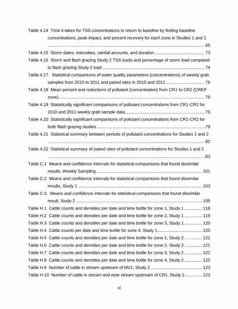
Table 4.14 Time it takes for TSS concentrations to return to baseline by finding baseline

concentrations, peak impact, and percent recovery for each zone in Studies 1 and 2

...................................................................................................................................... 65

Table 4.15 Storm dates, intensities, rainfall amounts, and duration ........................................... 73

Table 4.16 Storm and flash grazing Study 2 TSS loads and percentage of storm load compared

to flash grazing Study 2 load ....................................................................................... 74

Table 4.17 Statistical comparisons of water quality parameters (concentrations) of weekly grab

samples from 2010 to 2011 and paired sites in 2010 and 2011 ................................. 76

Table 4.18 Mean percent and reductions of pollutant (concentration) from CR1 to CR2 (CREP

zone)............................................................................................................................. 79

Table 4.19 Statistically significant comparisons of pollutant concentrations from CR1-CR2 for

2010 and 2011 weekly grab sample data .................................................................... 79

Table 4.20 Statistically significant comparisons of pollutant concentrations from CR1-CR2 for

both flash grazing studies ............................................................................................ 79

Table 4.21 Statistical summary between periods of pollutant concentrations for Studies 1 and 2

...................................................................................................................................... 82

Table 4.22 Statistical summary of paired sites of pollutant concentrations for Studies 1 and 2

.................................................................................................................................... ..83

Table C.1 Means and confidence intervals for statistical comparisons that found dissimilar

results, Weekly Sampling ........................................................................................... 101


results, Study 1 .......................................................................................................... 103


result, Study 2 ............................................................................................................ 105

Table H.1 Cattle counts and densities per date and time bottle for zone 1, Study 1 ............... 118



Table H.4 Cattle counts per date and time bottle for zone 4, Study 1 ...................................... 120





Table H.9 Number of cattle in stream upstream of MV1, Study 2 ............................................ 123

Table H.10 Number of cattle in stream and near stream upstream of CR1, Study 2 ............... 123

1

1 Introduction

Under the Clean Water Act of 1972, the United States Environmental Protection Agency

(USEPA) established goals to clean up the nation’s water systems through programs such as

total maximum daily loads (TMDLs). A TMDL is the calculation of the maximum amount of a

pollutant allowed in a water body that meets water quality standards by allocating loads from

point sources and nonpoint sources (NPS) (USEPA, 2008). Because point sources are easier

to trace, they have been the primary focus in pollutant control efforts. NPS pollution does not

have a clearly defined inlet point and comes from many sources, from runoff of urban parking

lots to the impacts of roaming livestock in streams.

As livestock enter water bodies such as streams, they disturb the riparian habitat and introduce

pollutants such as bacteria into the system. The first attempt in regulating the negative impacts

of cattle was through the Taylor Grazing Act of 1934. This act limited the number of cattle per

pasture area and promoted rangeland ecosystems through the installation of fencing and

vegetation management (BLM, 2011).

The two primary ways in which cattle affect stream water quality are through direct cattle

presence in the stream corridor and from overland flow during storm events carrying NPS

pollutants to the stream. There are many different best management practices (BMPs) that help

reduce direct deposition, overland flow, or both. One practice that is widely used is establishing

cattle streamside exclusion fencing because approximately 80 percent of riparian damage is

due to cattle presence (Agouridis et al., 2004a). Fencing protects the riparian habitat by

restricting cattle presence while still allowing the farmer to utilize the land around the water.

Although cattle streamside fencing has been proven to reduce pollutant concentrations in water

systems, the impact is not well documented because it is often costly to quantify (Zeckoski et

al., 2007).

Farmers find it desirable to have the option to use ‘flash grazing’ to utilize forage or to benefit

from streamside shade at a limited number of times through the year. Flash grazing is defined

as the short-term introduction of cattle into pastures areas at a higher than normal density to

quickly harvest vegetation. Under the Conservation Reserve Enhancement Program (CREP),

farmers are prohibited from allowing cattle into the riparian areas, thus restricting flash grazing

(James et al., 2007). Through this study, the effects of flash grazing on stream water quality

were analyzed to help determine if flash grazing could be considered as an accepted

2

management practice which could provide farmers with additional cattle and land management

opportunities.

This research focuses on cattle exclusion practices in the Shenandoah Valley, Virginia in

Rockingham County near Keezletown, Virginia. The stream systems are part of the Potomac

River Basin which ultimately flows into the Chesapeake Bay.

The main objective of this project is to assess the impact of short-term grazing practices on

water quality parameters in agricultural headwater streams. To define the objective further, the

following sub-objectives were evaluated:

Determine if short-term introduction of cattle significantly increases pollutant

concentrations

Quantify the number of cattle that increase turbidity above a baseline concentration

Calculate time for peak concentrations to return to baseline

Determine if pollutant loads from a flash grazing event are larger than loads from storm

events

Assess differences in stream water quality between reaches with no cattle, free access

cattle, and flash-grazing access over a two-year sampling period

Compare changes of water quality parameter concentrations through permanently

excluded and flash grazing reaches

3

2 Literature Review

2.1 Best Management Practices

A best management practice is a generic term for a practice that is implemented or installed

with the intent of reducing or mitigating pollution. According to the USEPA (2003), there are

three types of livestock BMPs designed to improve water quality: structural (e.g. stream

fencing), vegetative (e.g. riparian buffers), and management (e.g. rotational grazing). These

three types of BMPs reduce NPS pollution in three ways: reducing carrier mass and direct

pollutant concentrations, reducing overland flow concentrations to water bodies such as

streams, and remediation (USEPA, 2003). Along with reducing NPS pollution, BMPs have other

benefits such as improving long-term soil productivity and reducing production costs (Johengen

et al., 1989).

Some best management practices such as cattle exclusion fencing also promote the use of

other BMPs. Such BMPs are called indicator best management practices because fencing

implies that other BMPs such as off-stream waters may also need to be implemented in a given

production system (Benham et al., 2005).

BMPs must be implemented and maintained properly to be effective. In order to determine

BMP effectiveness, extensive and costly monitoring programs are often used. Therefore, there

is a need to establish a systematic approach to evaluating such BMPs in order to improve

quality. Understanding the effectiveness of BMPs includes knowing inputs into the system from

non-agricultural sources such as urban straight pipes that may mask the inputs from agricultural

lands. It is also important to understand the variability among each site. Since no two sites are

the same, it is crucial to research how each site behaves individually in order to implement the

best BMP (Robillard et al., 1992).

2.2 Buffers

A buffer is the area between a water body and a pollutant source. In agricultural settings, a

buffer is designed to reduce the amount of pollutants entering a stream and is often vegetated

with a variety of grasses, shrubs, and trees. Streamside cattle fencing creates a buffer which

prevents cattle trampling, allowing for riparian vegetation to thrive.

To help promote the installation of buffers, in 1985 the United States Department of Agriculture

established the Conservation Reserve Enhancement Program (CREP) which provides land

4

owners a cost-share for renting their land for conservation practices (Sweeney and Blaine,

2007). Through this program, the government rented approximately 45 million acres of highly

erodible land to establish a natural ecosystem to reduce transport of sediment and excess

nutrients from 10 to 85 percent depending on width and type of vegetation (Sweeney and

Blaine, 2007).

When installing streamside fencing or growing a vegetative buffer, a major concern is often how

wide or long should it be to be most effective. Research is being done to quantify the

effectiveness of different types of buffers at specified widths to prevent certain pollutants from

entering a water body (examples found below). The most effective width optimizes the buffer

area as well as the percent reduction of pollutant loads. It is also important that the buffer is

cost-effective for famers in order to optimize land and cattle management. A large distance

between the stream and pasture reduces the amount of useable land for the cattle which may

create a need for additional, costly feed.

Studies try to optimize the effectiveness of BMPs and provide varying results and suggestions

since every site is different. For example, Vidon et al. (2008) found that when monitoring two –

130 meter reaches, one buffered and one not buffered, there were concentration reductions in

nitrate, suspended solids, and fecal coliform. Scrimgeour and Kendall (2002) found that even

buffer widths of 5 to 12 feet can improve stream water quality, benthic macroinvertebrates, and

groundwater quality. Another study discovered that buffers should be the same width as the

width of the cattle area in the uplands; however, the same study found that with high infiltration

rates represented by a sand surface, a 1.37 meter buffer can reduce bacteria by 95 percent

(Larsen et al., 1994).

With cattle exclusion fencing, a riparian buffer is naturally established as native vegetation

thrives. Although the widths, lengths, and vegetation may vary, buffers are still a very effective

way of reducing pollutant concentrations of overland flow into streams (Hughes, 2008).

2.3 Animal Stocking Density

Proper cattle-stocking density is critical to ensure forage and nutrients availability. Increasing

cattle density (# of animals per unit area) puts more strain on the food and water supply of the

landscape. Along with a decrease in forage availability, higher cattle densities increase fecal

matter in the pasture.

5

One study in New York, which reviewed phosphorus concentrations for free-range cattle, found

that the number of cattle in each pasture was proportional to the number of cowpies that were

found near streams. Similarly, the largest herd produced more cowpies than the smaller herd

(James et al., 2007). Although this is expected, it shows that managing the proper number of

cattle may be important to water quality issues as well.

Densities also help define the influence livestock will have on water habitats. A large number of

cattle in a small, confined area have the potential to be more detrimental to water quality versus

a small number of cattle in a large area. Buckhouse and Gifford (1976) found that at a density

of 2 ha/aum (hectares/animal unit per month), there were no significant public health hazards

due to fecal coliform in runoff.

2.4 Pasture Characteristics

There are many factors that affect how much time cattle spend in the stream such as shade,

water availability, or pasture size and shape. A smaller pasture with stream access will increase

the time cattle are in-stream then when compared to a larger, similar pasture (Russell, 2010).

Even if the pasture is the same size, the shape of the pasture can also affect cattle behavior

and movement within water habitats (Russell, 2010). A third factor can be the length of stream

within the pasture and the spatial reference of the stream. For example, a stream at the edge of

the pasture may have less cattle impact than a stream that cuts a pasture in half because cattle

will have to cross it to get to the other half of the pasture for forage. The greater the length of

stream in the pasture, the more area the cattle have to enter.

In livestock pastures, riparian areas tend to host the majority of the trees because pastures are

often excavated for crop production and easy cattle management. Livestock are likely to

congregate for longer time periods in areas with trees for shade during the hot summer season

or shelter during storm events. Because the density and time of cattle in the stream increases,

streams are particularly vulnerable, especially when streamside exclusion fencing is not

present. Providing trees for shade and shelter outside of riparian areas may reduce the time

cattle spend in the stream and the number of cattle in the stream without the need for exclusion

fencing (Zeckoski et al., 2007).

2.5 Alternative Water

If streams are the sole source of water for livestock, an alternative water source needs to be

provided when streamside fencing is installed. Without fencing and an alternative drinking

6

source, livestock must enter the stream to drink. While in the stream, cattle are likely to

defecate, which adversely impacts water quality (Gary et al., 1983). One study found that when

troughs were available, total suspended solids (TSS) and E. coli bacteria were reduced by 95%,

dissolved phosphorus by 85%, and total phosphorus by 57%(Franklin et al., 2009).

Providing off-stream water can be a very effective way for diverting cattle away from streams. A

study in Virginia found that the time cattle spend in the stream zone decreased in-stream time

from 13 minutes/day to 6 minutes/day when alternative water was provided (Bewsell et al.,

2007). Other studies have found that off-stream water reduced the time cattle spend in streams

by 99% after feeding and up to 80% for other times in the day (Miner et al., 1992).

Temperature can also be a key factor as to how much time cattle spend in streams versus their

need for a water supply. One study found that when the outside temperature is between 62 and

72oF, off-stream waterers reduced the time cattle spent in streams by 63% (Franklin et al.,

2009). However, when the environment is considered stressful (> 72oF) the availability of off-

stream waterers had no effect on time cattle spent in-stream (Franklin et al., 2009). In stressful

conditions, cattle use the stream for more than just drinking purposes. The water, as well as

possible riparian trees, aid in cooling the animal.

When given two water sources, cattle tend to go with the source that is closest or the one they

are the most habituated toward. However, when clean off-stream water is available, cattle will

drink that water over other water of poor quality, so providing an alternative water supply may

decrease the amount of time livestock spend in water bodies for drinking (Vallentine, 1989).

One way to provide clean water to livestock is to pump groundwater into troughs in upland

areas instead of taking water from the stream (Bewsell et al., 2007).

2.6 Specified Entrance Points

Instead of fencing cattle entirely out of the stream, planned entrance points may be a beneficial

option when alternative water is not available or when cattle need to cross the stream to get to

other pastures. Creating an alternative entrance point can reduce the amount of time cattle are

in the stream and reduce cattle influences along the entire reach (Russell, 2010). Thus, the

amount of feces and urine deposited directly into the stream is reduced as well as the potential

for erosion and nutrients to be re-suspended (Russell, 2010).

Cattle are habitual animals: they tend to walk in areas they normally walk and enter streams in

the same location each time. Agouridis et al. (2005) found that when cattle had free access to

7

an entire reach, they favored certain sections of a stream. These areas may represent places

with shade, easy access, or even a favorable stream bed material that is easy to traverse.

Stabilizing these favorable sections instead of fencing the entire reach may have a significant

positive improvement on water quality.

Alternative entrance points are often lined with a man-made material to stabilize the stream

banks and bed since there will be increased animal traffic in these areas. Stabilizing materials

can be made from a variety of materials and should be selected based on site-specific

characteristics (Russell, 2010).

2.7 Cattle Impacts on the Stream Environment

Cattle are a major source of non-point pollution in agricultural watersheds (Vesterby and Krupa,

1997). Livestock can introduce many pollutants into the aquatic ecosystem including bacteria,

nutrients, and sediment (from trampling stream banks and disturbing the stream-bed). Bacteria

can enter the stream from cattle direct deposition of feces and in runoff during storm events.

Cattle also tear away at the natural riparian habitat through trampling the ground and uprooting

vegetation. Livestock streamside exclusion fencing has the potential to eliminate direct

deposition and reduce pollutants in overland flow by providing the opportunity for vegetation in

the fenced riparian corridor to thrive.

2.7.1 Stream Bed and Bank Impacts

When cattle have unrestricted stream access, they trample stream banks increasing the

potential for erosion which in return degrades water quality. Streambank trampling can impact

stream channel morphology, hydrology, in-stream and bank vegetation, and aquatic and riparian

wildlife (Miller et al., 2010). Cattle can also degrade the banks by scratching their bodies

against any protruding ground. Smoothed bare areas and eroding-terrace cuts can be

explained by this scratching (Peppler and Fitzpatrick, 2006).

Streambank sediment loss increases erosion and re-suspends bacteria and other nutrients that

were trapped in the soil (Franklin et al., 2009). When the soil erodes, unstable ground is left

which provides a poor environment for riparian vegetation to thrive. Therefore, not only are the

cattle re-suspending the sediment, but since the vegetation stabilizes the soil, even more

sediment erodes away with a lack of vegetation. Banks get eroded when the forces of the

flowing water are greater than the forces holding the soil in place, which is also known as being

in a state of disequilibrium (Reynaud et al., 2003).

8

Vegetation reduces the force the water exerts on the soil as well as increases the forces holding

the soil together. Banks become unstable under conditions of easily eroded soil with very little

vegetation and smaller particle sizes (Miller et al., 2010). With the exclusion of livestock, native

vegetation will have the chance to grow and thrive near the stream. Exclusion will also help

introduce vegetation that needs a longer time to get established such as shrubs and trees

(Miller et al., 2010).

In a study conducted in Lancaster County, Pennsylvania, Scrimgeour and Kendall (2002) found

that the most prominent observation of eliminating cattle access to streams was increased

vegetation along the stream channel with the stability of the assessed stream habitats

increasing from 74 to 94% compared to stream habitats with cattle access. Scimgeour and

Kendall (2002) also found that sediment yields decreased post-installation of cattle fencing

during low-flows but significantly lowered sediment concentrations during storm flow. Post

fencing, the overall yield reduction of suspended sediments was 46% at the outlet. When

comparing yields to the control site, the outlet had an overall reduction of 37% while the further

upstream point had a reduction of 44% of suspended sediments.

A study done in Kentucky used two bedrock streams to compare cross-sectional areas of cattle

access and fenced stream sections. Along each stream were three different levels of cattle

access - BMP system (alternative water) and exclusion fencing, BMP system only (just

alternative water), and free access/control (Agouridis et al., 2005). Through this study, it was

found that streambank erosion and soil loss is significant with treatment type, cattle in and near

the stream, and flow. There was not much significant difference between the two cattle-

restricted sites; however, there was a significant difference between those two treatments and

the free cattle access site (Agouridis et al., 2005). It was also found that more damage to the

stream was during wet periods which can influence cross-sections within a few hours to a few

days after a wet period (Agouridis et al., 2005).

The suspension of sediment into the water column can also be transported downstream causing

a more turbid stream. High turbidity decreases the amount of sunlight that reaches the stream

bed where aquatic vegetation lives and grows. Without the vegetation, organisms such as

macroinvertebrates and fish will decrease in numbers due to an unhealthier habitat.

Another reason it is important that livestock do not cut back the banks is that it changes the

channel morphology of the stream. Streams naturally tend to meander through eroding banks;

9

however, when cattle degrade the banks, it disrupts this natural pattern and increases the

erosion process (Peppler and Fitzpatrick, 2006).

When determining the sources of high sediment yields in the stream, the entire drainage area

should be analyzed. Cattle can break up soils on the landscape that can be transported through

overland flow to the water body. One study in Australia found that cattle exclusion on the

watershed scale reduced sediment concentrations up to 90% (Vidon et al., 2008). Also, more

total suspended solids can be found in areas of a long history of waste application due to the

buildup of residual organic material on the surface of the soil (Soupir, 2003).

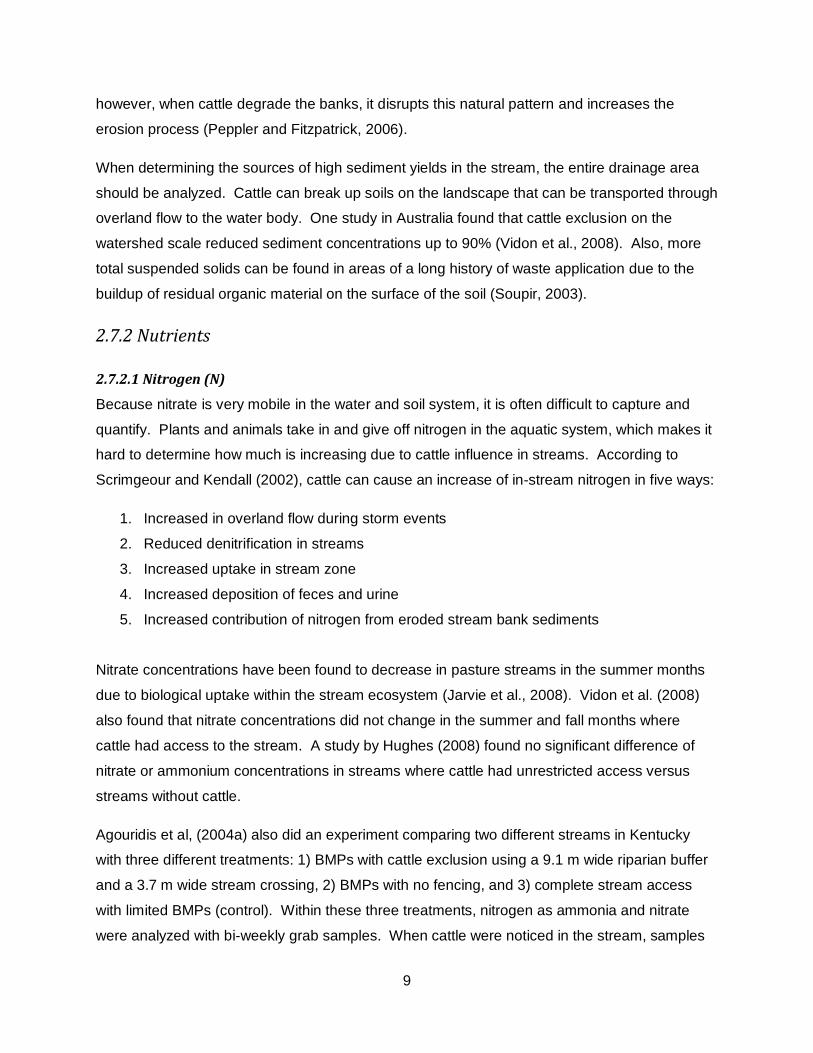
2.7.2 Nutrients

2.7.2.1 Nitrogen (N)

Because nitrate is very mobile in the water and soil system, it is often difficult to capture and

quantify. Plants and animals take in and give off nitrogen in the aquatic system, which makes it

hard to determine how much is increasing due to cattle influence in streams. According to

Scrimgeour and Kendall (2002), cattle can cause an increase of in-stream nitrogen in five ways:

1. Increased in overland flow during storm events

2. Reduced denitrification in streams

3. Increased uptake in stream zone

4. Increased deposition of feces and urine

5. Increased contribution of nitrogen from eroded stream bank sediments

Nitrate concentrations have been found to decrease in pasture streams in the summer months

due to biological uptake within the stream ecosystem (Jarvie et al., 2008). Vidon et al. (2008)

also found that nitrate concentrations did not change in the summer and fall months where

cattle had access to the stream. A study by Hughes (2008) found no significant difference of

nitrate or ammonium concentrations in streams where cattle had unrestricted access versus

streams without cattle.

Agouridis et al, (2004a) also did an experiment comparing two different streams in Kentucky

with three different treatments: 1) BMPs with cattle exclusion using a 9.1 m wide riparian buffer

and a 3.7 m wide stream crossing, 2) BMPs with no fencing, and 3) complete stream access

with limited BMPs (control). Within these three treatments, nitrogen as ammonia and nitrate

were analyzed with bi-weekly grab samples. When cattle were noticed in the stream, samples

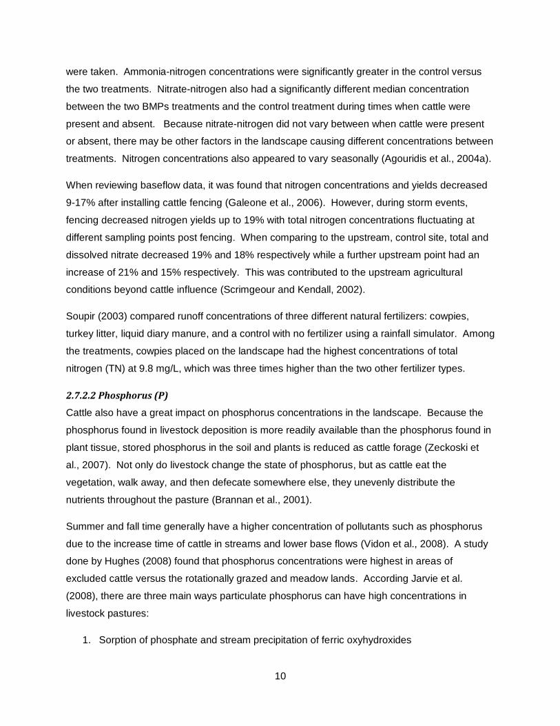
10

were taken. Ammonia-nitrogen concentrations were significantly greater in the control versus

the two treatments. Nitrate-nitrogen also had a significantly different median concentration

between the two BMPs treatments and the control treatment during times when cattle were

present and absent. Because nitrate-nitrogen did not vary between when cattle were present

or absent, there may be other factors in the landscape causing different concentrations between

treatments. Nitrogen concentrations also appeared to vary seasonally (Agouridis et al., 2004a).

When reviewing baseflow data, it was found that nitrogen concentrations and yields decreased

9-17% after installing cattle fencing (Galeone et al., 2006). However, during storm events,

fencing decreased nitrogen yields up to 19% with total nitrogen concentrations fluctuating at

different sampling points post fencing. When comparing to the upstream, control site, total and

dissolved nitrate decreased 19% and 18% respectively while a further upstream point had an

increase of 21% and 15% respectively. This was contributed to the upstream agricultural

conditions beyond cattle influence (Scrimgeour and Kendall, 2002).

Soupir (2003) compared runoff concentrations of three different natural fertilizers: cowpies,

turkey litter, liquid diary manure, and a control with no fertilizer using a rainfall simulator. Among

the treatments, cowpies placed on the landscape had the highest concentrations of total

nitrogen (TN) at 9.8 mg/L, which was three times higher than the two other fertilizer types.

2.7.2.2 Phosphorus (P)

Cattle also have a great impact on phosphorus concentrations in the landscape. Because the

phosphorus found in livestock deposition is more readily available than the phosphorus found in

plant tissue, stored phosphorus in the soil and plants is reduced as cattle forage (Zeckoski et

al., 2007). Not only do livestock change the state of phosphorus, but as cattle eat the

vegetation, walk away, and then defecate somewhere else, they unevenly distribute the

nutrients throughout the pasture (Brannan et al., 2001).

Summer and fall time generally have a higher concentration of pollutants such as phosphorus

due to the increase time of cattle in streams and lower base flows (Vidon et al., 2008). A study

done by Hughes (2008) found that phosphorus concentrations were highest in areas of

excluded cattle versus the rotationally grazed and meadow lands. According Jarvie et al.

(2008), there are three main ways particulate phosphorus can have high concentrations in

livestock pastures:

1. Sorption of phosphate and stream precipitation of ferric oxyhydroxides

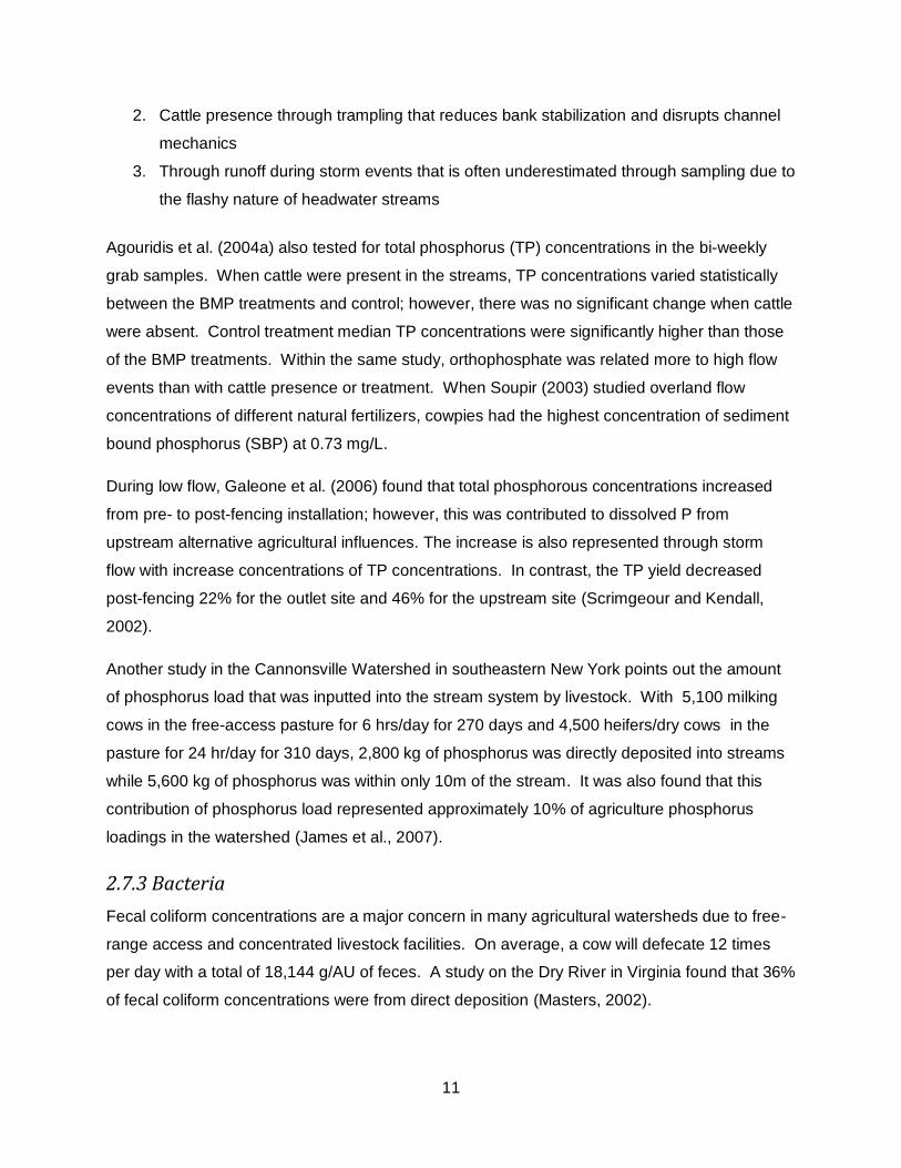
11

2. Cattle presence through trampling that reduces bank stabilization and disrupts channel

mechanics

3. Through runoff during storm events that is often underestimated through sampling due to

the flashy nature of headwater streams

Agouridis et al. (2004a) also tested for total phosphorus (TP) concentrations in the bi-weekly

grab samples. When cattle were present in the streams, TP concentrations varied statistically

between the BMP treatments and control; however, there was no significant change when cattle

were absent. Control treatment median TP concentrations were significantly higher than those

of the BMP treatments. Within the same study, orthophosphate was related more to high flow

events than with cattle presence or treatment. When Soupir (2003) studied overland flow

concentrations of different natural fertilizers, cowpies had the highest concentration of sediment

bound phosphorus (SBP) at 0.73 mg/L.

During low flow, Galeone et al. (2006) found that total phosphorous concentrations increased

from pre- to post-fencing installation; however, this was contributed to dissolved P from

upstream alternative agricultural influences. The increase is also represented through storm

flow with increase concentrations of TP concentrations. In contrast, the TP yield decreased

post-fencing 22% for the outlet site and 46% for the upstream site (Scrimgeour and Kendall,

2002).

Another study in the Cannonsville Watershed in southeastern New York points out the amount

of phosphorus load that was inputted into the stream system by livestock. With 5,100 milking

cows in the free-access pasture for 6 hrs/day for 270 days and 4,500 heifers/dry cows in the

pasture for 24 hr/day for 310 days, 2,800 kg of phosphorus was directly deposited into streams

while 5,600 kg of phosphorus was within only 10m of the stream. It was also found that this

contribution of phosphorus load represented approximately 10% of agriculture phosphorus

loadings in the watershed (James et al., 2007).

2.7.3 Bacteria

Fecal coliform concentrations are a major concern in many agricultural watersheds due to free-

range access and concentrated livestock facilities. On average, a cow will defecate 12 times

per day with a total of 18,144 g/AU of feces. A study on the Dry River in Virginia found that 36%

of fecal coliform concentrations were from direct deposition (Masters, 2002).

12

When animal feces is deposited on land, bacteria has a much higher die-off rate than when

deposited directly in the stream; therefore, direct deposition is more of a source of fecal coliform

than that of over-land flow (Masters, 2002). However, bacteria can live within the soil column

for 13-20 days, live for months attached to sediment and solids, and live up to a year in the

livestock feces (Masters, 2002). Buckhouse and Gifford (1976) found that coliform bacteria can

live for at least a summer season in low intensive sun. The dying rates of fecal coliform were

also found to be much shorter in soils with a higher percentage of clay particles (Howell et al.,

1996).

With resuspension of sediment through cattle trampling, bacteria can also be resuspended into

the water column degrading water quality. In a square meter area, from 1-760 million fecal

coliform organisms can get resuspended when cattle enter the stream (Larsen et al., 1994).

However, Buckhouse and Gifford (1976) also found that the radial area of one meter around a

fecal deposition on land is at risk of fecal contamination and not beyond that distance; therefore,

only piles near or in stream may contribute to water quality contamination of fecal coliform.

One study found that cattle in-stream produced 12.5 times greater fecal coliform than a stream

with where no cattle are present with concentrations varying from 380-20,000 FC/100 mL with

cattle present and less than 250 FC/100 mL with no cattle present (Masters, 2002). When

cattle were introduced, concentrations increased to greater than 10,000 FC/100 mL, which is 40

times higher prior to cattle inclusion (Masters, 2002). It takes a maximum of several months for

the bacteria to go back down to base level concentrations after cattle are removed (Larsen et

al., 1994).

Soupir (2008) found that plots with cowpies had the highest flow-weighted concentrations of E.

coli at 200,000 cfu/100ml and fecal coliform at 234,000 cfu/100ml at baseflow conditions.

Similarly, during rainfall events, the cowpie treatment had the highest concentration of bacteria

with E. coli ranging from 37,000-300,000 cfu/100ml and fecal coliform ranging from 65,000-

300,000 cfu/100ml.

Bacteria are also a water quality issue for TMDLs. In order to understand why a stream is

impaired, a watershed evaluation of different sources is assessed. The Big Otter River in

Virginia had a TMDL for fecal coliform in 2001. The 30-day geometric mean Virginia State

standard for fecal coliform was 200 cfu/100ml with an instantaneous standard of 1000 cfu/100ml

(Brannan et al., 2001). With a 5% margin of safety (MOS) of 10 cfu/100ml, the 30-day

geometric mean standard becomes 190 cfu/100ml (Follett and Hatfield, 2001, pp. 17-43).

13

However, when the watershed is modeled for a 100% reduction of anthropogenic straight pipes

and direct defecation from cattle, the 30-day geometric mean will still not decrease to 190

cfu/100ml (Brannan et al., 2001).

2.7.4 pH and Salinity

The pH can also be considered an important water quality indicator but is not often mentioned in

studies because it generally does not fluctuate significantly. The pH in both BMP treatments in

Agouridis (2004a) study was significantly lower than the pH in the control treatment when cattle

were both absent and present. Because pH did not change significantly from cattle being

present or absent, other external factors can be attributed for changes in pH other than cattle

activity.

Although salinity is typically not affected by cattle exclusion, it affects cattle behavior, which in

turn could affect cattle presence in the stream as well as health of the animal. Concentrations

of 7,000 ppm of soluble salts is not harmful to an animal but caused them to drink less and

potentially spend less time in the stream channel (Embry et al., 1959). Conversely, a

concentration of 10,000 ppm could be toxic to livestock (Shukla, 2000).

2.7.5 Benthic Macroinvertebrates

Benthic macroinvertebrates (macros) are the larva stage of many insects that live on the stream

bed. They are often used as a sign of water quality such as the Virginia Save Our Streams

Program (VA SOS) because certain insects are very intolerant to certain water conditions. A

healthier stream is comprised of a variety of tolerant and intolerant insects. Macroinvertebrates

are often studied because collection and identification of the bugs are easy and require few

equipment and people (Frondorf, 2001).

Macroinvertebrates are generally very abundant in streams and rivers, much more so than other

biological indicators such as fish (Frondorf, 2001). They also are good indicators of stress on

the aquatic environment because they are not very mobile as opposed to fish which can swim

around to various parts of the stream or river (MDDNR, 2004). Because of the short life span of

macroinvertebrates, they quickly respond to pollutants and their stressors, which give scientists

a snapshot of the water’s quality (Frondorf, 2001). Stressors include nutrients, sediment, and

organic and inorganic toxicants (MDDNR, 2004). An excess amount of sediment in the aquatic

ecosystem can put stress on the benthos by changing the water’s movement and decreasing

14

food quality (Frondorf, 2001). Once evaluations are made based on the macroinvertebrates,

best management practices can be recommended to improve water quality.

For these reasons, benthic macroinvertebrates are also used when evaluating water quality

improvements pre- and post-cattle fencing. Galeone et al. (2006) found that post fencing, the

quality of benthic macroinvertebrates improved overall. This improvement could be due to the

increase of streamside vegetation that allows for more trapping of sedimentation, which can

increase habitat for macroinvertebrates. When comparing the control sites to the downstream,

outlet location, the benthic macroinvertebrates improved in all indices categories but only three

out of the five biological indicator indices for the upstream sites.

2.8 Flash Grazing

There are many different ways to manage livestock such as mob grazing, controlled grazing,

deferred grazing, rotational grazing, and flash grazing. Because it is not economically feasible

or realistic to fence separate riparian pastures for rotational grazing, it is important to develop a

plan for livestock management that includes cattle and forage distributions (Platts and Nelson,

1985). Agouridis (2004b) outlined three practices for acceptable grazing in riparian areas:

1. Limiting time of grazing

2. Limiting livestock density

3. Limiting livestock time in pastures when banks are most susceptible to damage

Understanding the impacts of flash grazing can provide additional management opportunities for

farmers and land owners. Under the CREP program, managers are not allowed to let cattle

graze within the cost-shared fencing. Providing the opportunity to allow cattle to feed on the

riparian vegetation and/or to gain shade under certain conditions may make managers more

amenable on installing exclusion fencing. As research continues, flash grazing has the

opportunity to be considered a BMP with the installation of streamside exclusion fencing as

compared to continuous free access cattle. Already in Minnesota, the United States

Department of Agriculture (USDA) has declared rotational animal densities as a best

management practice and helps farmers develop grazing and livestock management plans


One study in Minnesota looked at the impacts of continuous grazing (CG), short-duration

grazing (SDG), and no grazing (NG). Continuous grazing sites had free range cattle without

any fencing. Short-duration grazing sites rotated cattle within pastures and paddocks to utilize

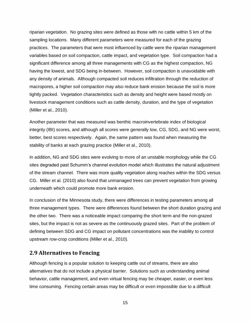
15

riparian vegetation. No grazing sites were defined as those with no cattle within 5 km of the

sampling locations. Many different parameters were measured for each of the grazing

practices. The parameters that were most influenced by cattle were the riparian management

variables based on soil compaction, cattle impact, and vegetation type. Soil compaction had a

significant difference among all three managements with CG as the highest compaction, NG

having the lowest, and SDG being in-between. However, soil compaction is unavoidable with

any density of animals. Although compacted soil reduces infiltration through the reduction of

macropores, a higher soil compaction may also reduce bank erosion because the soil is more

tightly packed. Vegetation characteristics such as density and height were based mostly on

livestock management conditions such as cattle density, duration, and the type of vegetation


Another parameter that was measured was benthic macroinvertebrate index of biological

integrity (IBI) scores, and although all scores were generally low, CG, SDG, and NG were worst,

better, best scores respectively. Again, the same pattern was found when measuring the

stability of banks at each grazing practice (Miller et al., 2010).

In addition, NG and SDG sites were evolving to more of an unstable morphology while the CG

sites degraded past Schumm’s channel evolution model which illustrates the natural adjustment

of the stream channel. There was more quality vegetation along reaches within the SDG versus

CG. Miller et al. (2010) also found that unmanaged trees can prevent vegetation from growing

underneath which could promote more bank erosion.

In conclusion of the Minnesota study, there were differences in testing parameters among all

three management types. There were differences found between the short duration grazing and

the other two. There was a noticeable impact comparing the short term and the non-grazed

sites, but the impact is not as severe as the continuously grazed sites. Part of the problem of

defining between SDG and CG impact on pollutant concentrations was the inability to control

upstream row-crop conditions (Miller et al., 2010).

2.9 Alternatives to Fencing

Although fencing is a popular solution to keeping cattle out of streams, there are also

alternatives that do not include a physical barrier. Solutions such as understanding animal

behavior, cattle management, and even virtual fencing may be cheaper, easier, or even less

time consuming. Fencing certain areas may be difficult or even impossible due to a difficult

16

landscape, so an alternative may be necessary for farm managers in order to protect riparian

areas.

2.9.1 Animal Behavior

Through the studies and teachings of Dr. Temple Grandin, options of training cattle versus

forcing cattle are being understood. Most of the processes Dr. Grandin proposes involves

handling cattle in shoots and facilities; however, the same ideals can be applied to pasture

cattle as well (Grandin, 2011).

Cattle behavior is important to understand because it can give an insight as to how

management can hone in and create the best management decisions for cattle health,

productivity, and the environment. One behavioral adaptation noticed by Agouridis et al.

(2004b) was that cattle often avoided trees even during rainfall events whereas the typical

perception is that cattle use the trees as shelter from the rain. Agouridis et al., (2004b) also

found that the amount of time cattle spent in streams was most related to the amount of

daylight. The increase could be the result of more daylight for grazing or higher temperatures.

As one study found, as air temperature got higher, the amount of time cattle spent near streams

grew (Parsons et al., 2003).

2.9.2 Cattle Management

Understanding how to properly manage livestock numbers and eating habits may reduce the

amount of time cattle spend in streams and therefore may eliminate the need for fencing. For

example, a study done in the mountainous western United States found that cattle wandered

further away from the stream during the early parts of summer versus late summer (Parsons et

al., 2003). Grazing cattle in pastures with unfenced areas may be most beneficial in the early

summer because vegetation throughout the pasture in the early summer is often most desirable.

Therefore, cattle will roam more freely and not tend to favor the riparian areas that are luscious

throughout the summer. Managing cattle away from the riparian zone in early spring allows for

more growth of riparian during the summer season (Elmore and Kauffman, 1994). Platts and

Nelson (1985) found that in 23 out of the 25 observations, cattle used streamside vegetation

twice as much as vegetation in the uplands.

It was also found that the animals were the furthest from the stream in the early mornings and

gradually became closer and closer as the day progressed until late afternoon where they

moved further upland again. Because more cattle were found near the stream in early spring, it

17

was also found that there were more fecal piles that could contribute to poor water quality

(Parsons et al., 2003).

2.9.3 Virtual Fencing

Another alternative to a physical fence is the new and upcoming technology of a virtual fence. A

study in Australia researched the idea of creating boundaries using GPS technology. A virtual

fence was made with GPS points representing the fencing, and through satellite technology,

when cattle wearing the high-tech collar crossed the virtual fence, music started playing. If the

animal continued to walk further past the fence, a shock was given encouraging the cattle to go

back. Cattle were responsive to the method within an hour and remained stress free. Although

each collar is costly at approximately $50 per collar, it may be a beneficial alternative when a

physical fence is too challenging to install (Alison, 2007).

2.10 Stakeholders

Getting stakeholders involved in helping improve water quality is often difficult because of costs

and time involved in installing BMPs. With cost-share programs, stakeholders are responsible

for providing the upfront cost, full installation for BMPs, and any additional maintenance costs

including parts and labor (VADCR, 2011). Benham et. al (2005) created a five point scoring

system that measured BMPs based on quality, site selection, implementation, and maintenance.

Results showed that cost-share and noncost-share BMPs had no significant statistical

difference for indicator BMPs such as cattle exclusion fencing; however, the mean for the cost-

share BMPs were higher, resulting in a better overall score.

Because it is ultimately the stakeholders’ responsibility to install BMPs and keep it up to code, it

is important to understand stakeholder perception. Stakeholders in four different watersheds

were interviewed to determine their concerns with BMPs. The most important factor farmers

mentioned when questioned about exclusion fencing is stock management (Bewsell et al.,

2007). Cattle safety was designated the primary reason for fencing which might include fencing

around a dangerous pipe, for example. Other reasons stakeholders would install fencing are to

create farm boundaries, prevent cattle from getting trapped in a waterway, keeping cattle from

parasites in the water, and pressure from the community (Bewsell et al., 2007).

In preparing the VA Cooperative Extension publication, Zeckoski et al. (2007) interviewed

selected producers to understand their reason for either adopting or not adopting streamside

exclusion fencing. The main reasons for adopting streamside exclusion fencing was for benefits

18

such as getting the cost-share for providing off-stream water troughs. The second most popular

reason for installing fencing was because it is seen as the “right thing to do” for the environment.

Another advantage to fencing was that it allows for easier movement of cattle for rotational

grazing and to isolate individual cattle for veterinarian visits and other reasons (Zeckoski et al.,

2007). The most prominent reason for not adopting streamside exclusion fencing was because

it promotes the over-growth of vegetation between the stream and the fence (Zeckoski et al.,

2007). Some landowners find the natural, overgrowth of vegetation unsightly and cause a

nuisance to the fence. To make the buffer area between the fencing and stream more slightly,

one farmer flash grazed the riparian zone with sheep to “mow” the vegetation down (Zeckoski et

al., 2007).

2.10.1 Cattle Exclusion Economics

Although fencing is expensive, there can be a benefit as well as a cost. With implementation of

fencing and off-stream waterers, cattle weight and milk production can even increase. Over a

10 month period, one producer noticed a weight gain of 5-10% in their cattle with the installation

of streamside fencing (Zeckoski et al., 2007). Also, because the cattle are not drinking out of

water that may contain a high concentration of bacteria, diseases such as pink eye or mastitis

are also possibly reduced (Zeckoski et al., 2007). Salmonellosis and leptospirosis are the most

common diseases associated with contaminated water supplies (Buckhouse and Gifford, 1976).

A decrease in infection reduces the need for costly antibiotics and decreases the chance of

cattle lameness and death.

2.11 Summary

Although each stream may be considered a relatively small body of water, the regional impact of

many streams has great implications. Efforts to clean up the nation’s water systems include

farmers implementing livestock exclusion fencing to keep animals out of stream water. Through

the studies and articles mentioned, livestock have a large influence on not only water quality but

the ecosystem that surrounds them. Fencing may not be the perfect solution for every situation,

but through understanding animal behavior and good cattle management, smarter decisions can

be made to help clean up the waters that are very important to humans, animals, and the

ecosystem.

19

3 Methods

3.1 Site Descriptions

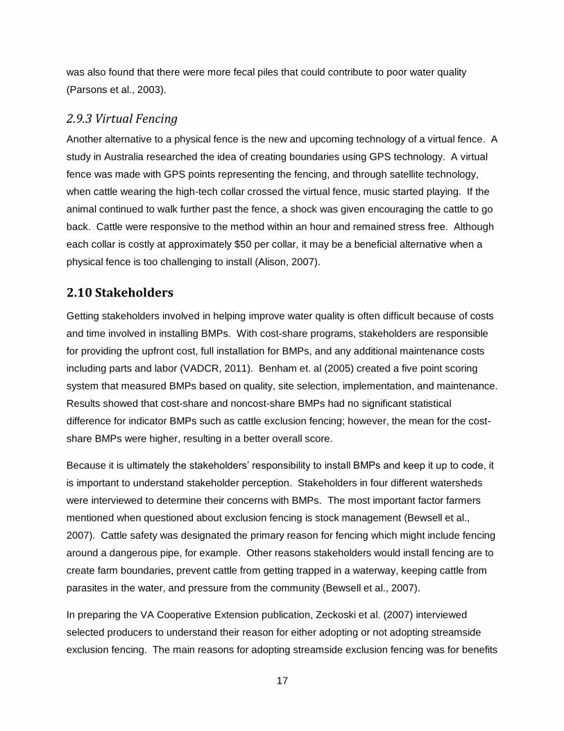
The project site is located in Rockingham County, Virginia (fig. 3.1). The site was chosen

because it was easily accessible, had permanent water samplers already in place, and the

operators were known to have previously flash grazed. Permanent fencing was installed on this

farm in 2009, so cattle were excluded from the streams for approximately two years before

sampling for this research was initiated. Cattle were also permanently excluded from the CREP

zone. However, the farmer occasionally allows cattle to flash graze the riparian zone outlined in

figure 3.1. While grazing in the riparian zone, cattle still have access to the pasture area at all

times.

Figure 3.1: Project site pasture area, riparian zone for flash grazing, and CREP fencing zone

located in Rockingham County, Virginia. (Source: Google Earth)

20

There were two streams: Cub Run (CR), and an unnamed tributary referred to here as

Mountain Valley Road (MV) tributary. Both streams were first order headwater streams where

MV flows into CR downstream of the study area. Cub Run eventually flows into the South Fork

Shenandoah River, then to the Potomac River, and ultimately into the Chesapeake Bay. Both

streams have unrestricted cattle access upstream of the study site. Upstream from the study,

MV flows through an old barnyard/farmstead presently used to pasture and winter-feed dairy

replacement heifers whereas upstream CR has beef cattle on pasture.

The MV tributary is a relatively straight, small stream with baseflow at approximately 5 L/s. As

seen in figure 3.2, tall grasses are the primary vegetation along the banks with only one tree

along the study reach. The reach length accessible during the flash grazing study is

approximately 356 m, and the MV reach from Mountain Valley Road to the confluence to Cub

Run is approximately 467 m.

Figure 3.2: Mountain Valley Road Tributary looking downstream (Source: Nancy Maschke)

Unlike MV, CR (fig. 3.3) has no major anthropogenic influences, and upstream of the free-range

cattle pasture is mostly forest. Cub Run has a greater flow than MV with a base flow of

approximately 9.5 L/s. The stream has a more natural meander than MV and the bed material is

cobble/stone, which promotes more riffles. Cub Run’s riparian zone has numerous hardwood

trees and does not have the heavy grass vegetation like MV. The total length of Cub Run within

the flash grazing zones is 444 meters, and the upstream CREP zone is 231 meters long.

21

Figure 3.3: Cub Run looking downstream (Source: Nancy Maschke)

3.2 Sampling

Three main types of sampling schemes were used: flash grazing, weekly, and storm. The

weekly and storm samples used in this research are part of a more comprehensive study. The

data from these samples were incorporated in this research project to get a broader

understanding of the impact that streamside fencing and cattle management practices may

have on water quality. The two flash grazing studies were sampled in July, 2011 (Study 1) and

August, 2011 (Study 2).

3.2.1 Flash Grazing Sampling

The flash grazing study was done in three periods: baseline, cattle influence, and recovery

referred to as periods 1, 2, and 3 respectively. Baseline (period 1) consisted of the first two

days of the study in order to determine pollutant concentrations before cattle were introduced to

the riparian area. The cattle influence period (period 2) was the following two days of sampling,

and cattle were able to move freely throughout the MV and CR flash grazing reaches as well as

adjacent pasture area. In order to quantify the time it takes pollutant concentrations to return to

a baseline level, the last day of the study (period 3) was sampled when cattle were prevented

from entering the streams.

As shown in figure 3.4, eight automated samplers (ISCOs) were used. Stations MV1, MV2,

CR1, and CR3 were permanent and were in the field for two years prior to this study. Stations

MV1b, CR2, CR2b, and CM were added in order to get a better representation of characteristics

within the study site.

22

Figure 3.4: Schematic of study site showing sampling locations

The newly added ISCOs were placed upstream of points of high priority. Because the farmer

had previously flash grazed, he had noticed that on MV, cattle tended to congregate at the

single tree on the reach. Therefore, an intermediate sample point, MV1b, was placed just

upstream of this tree. Because cattle were noticed to congregate at the confluence of MV and

CR, a sampling station, CM, was placed below this area. Additional areas of priority included

the main entrance point from the pasture to the riparian zone, CR2b, and the end entrance

upstream of the study site along Cub Run, CR2 (control).

Each ISCO was programmed to take a 120 ml subsample every 15 minutes. Each 1-L sample

bottle thus represented a composite of eight subsamples representing a two-hour composite.

The 15-minute interval was chosen in order to capture brief instances of cattle impact.

Sampling could not have been taken in increments less than 15 minutes due to ISCO

limitations. Two hour composites were used to ensure that spikes could be seen without having

to increase sample frequency.

Samples were removed from the ISCOs twice a day at 6:00 and at 16:00 and placed in ice filled

coolers for transport to the lab for pollutant concentration analysis. The ISCOs were also filled

with ice (fig. 3.5) during collection time periods to keep the samples cool.

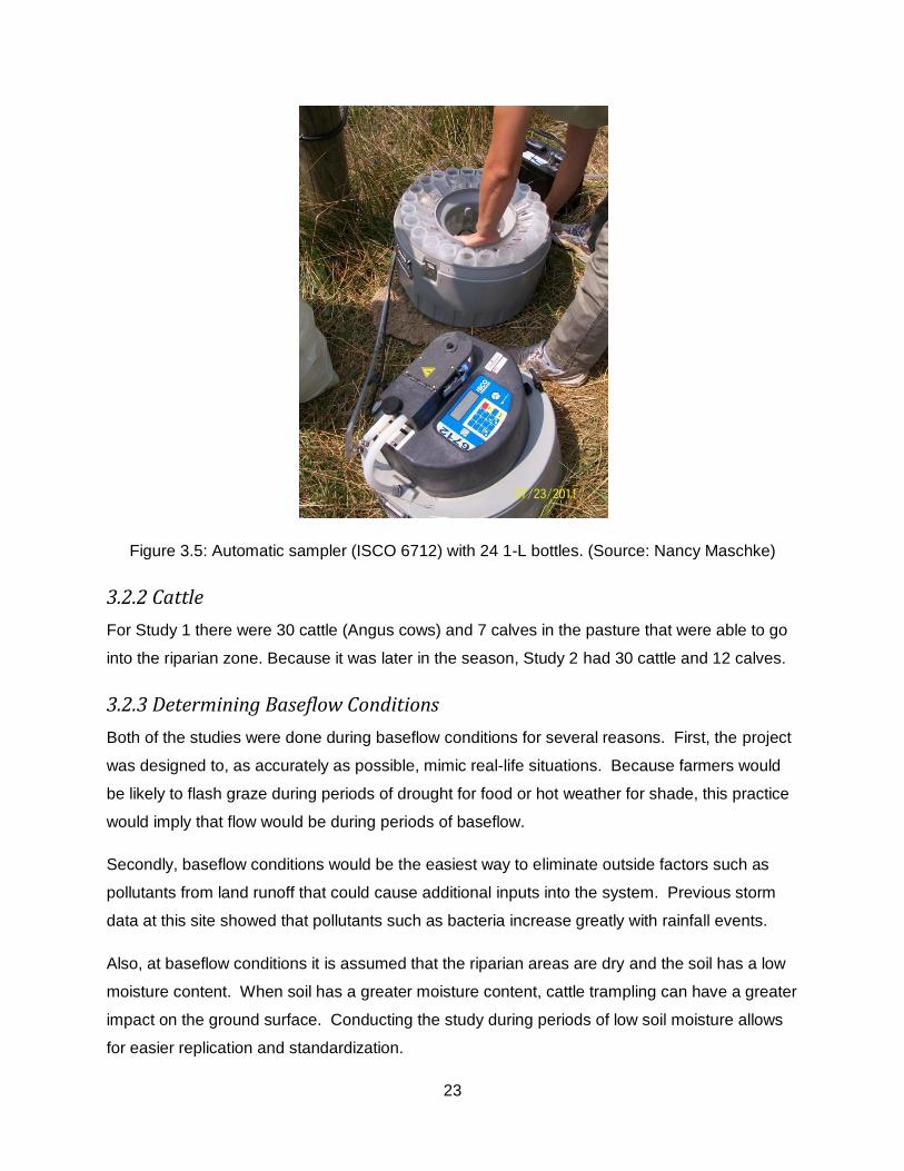
23

Figure 3.5: Automatic sampler (ISCO 6712) with 24 1-L bottles. (Source: Nancy Maschke)

3.2.2 Cattle

For Study 1 there were 30 cattle (Angus cows) and 7 calves in the pasture that were able to go

into the riparian zone. Because it was later in the season, Study 2 had 30 cattle and 12 calves.

3.2.3 Determining Baseflow Conditions

Both of the studies were done during baseflow conditions for several reasons. First, the project

was designed to, as accurately as possible, mimic real-life situations. Because farmers would

be likely to flash graze during periods of drought for food or hot weather for shade, this practice

would imply that flow would be during periods of baseflow.

Secondly, baseflow conditions would be the easiest way to eliminate outside factors such as

pollutants from land runoff that could cause additional inputs into the system. Previous storm

data at this site showed that pollutants such as bacteria increase greatly with rainfall events.

Also, at baseflow conditions it is assumed that the riparian areas are dry and the soil has a low

moisture content. When soil has a greater moisture content, cattle trampling can have a greater

impact on the ground surface. Conducting the study during periods of low soil moisture allows

for easier replication and standardization.

24

To ensure that baseflow conditions were present during the flash grazing studies, flow was

measured once during Study 1 (20 July 20 2011) and twice during Study 2 (16 and 19 August

16 2011). Flow was measured using the equal-width flow measurement technique with a Marsh

McBirney flow meter at each permanent ISCO station (MV1, MV2, CR1, and CR3) and at the

CM site to capture the flow downstream of the confluence.

3.2.4 Weekly Sampling

Grab samples were collected weekly, on the same day from June 7 2010 to 16 November 2010

and from 19 May 2011 to 16 August 2011. Samples were collected at the two permanent ISCO

stations on CR (CR1 and CR3) and two at MV (MV1 and MV2). The flash grazing CR1 was

labeled CR1b during the weekly grab samples. CR1a was an additional sample that was taken

just upstream of CR1b, which is also just upstream of the CR1 bridge cattle crossing. Sample

time was rotated each week in order to help capture any diurnal variations.

Weekly grab samples were collected mid-stream and mid-depth in a 250ml bottle for bacteria

analysis and in a 1-L bottle for TSS and nutrient analysis. From the 1-L sample, 2-10ml

subsamples were taken in scintillation vials for total nutrient analysis and 3-10ml filtered

subsamples were collected for dissolved nutrient analysis.

3.2.5 Storm Sampling

For the 2010 sampling season, four storms events were sampled on 13 July, 14 July, 27

September, and 30 September. For the 2011 season, five storms events were sampled on 17

May, 8 July, 15 August, 5 September, and 12 October. Storm samples were collected using the

four permanent ISCOs. When weather forecasters predicted a storm, the ISCOs were

programmed to take a subsample every 10 minutes with six subsamples in each 1-L bottle

comprising a one-hour composite.

3.2.6 Quality Control/Quality Assurance

Quality control and quality assurance checks were also run through various procedures of this

research to ensure the most accurate data. Appendix E and F show a comparison between the

manual grab samples and ISCO samples to ensure that the modes of collection are

comparable. Other checks such as determining residual bacteria in samplers and supplies can

be found in Appendix E and F as well.

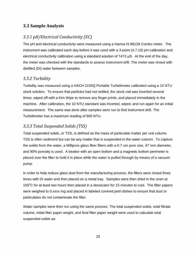
25

3.3 Sample Analysis

3.3.1 pH/Electrical Conductivity (EC)

The pH and electrical conductivity were measured using a Hanna Hi 98129 Combo meter. The

instrument was calibrated each day before it was used with a 3-point (4,7,10) pH calibration and

electrical conductivity calibration using a standard solution of 1413 μS. At the end of the day,

the meter was checked with the standards to assess instrument drift. The meter was rinsed with

distilled (DI) water between samples.

3.3.2 Turbidity

Turbidity was measured using a HACH 2100Q Portable Turbidimeter calibrated using a 10 NTU

stock solution. To ensure that particles had not settled, the stock vial was inverted several

times, wiped off with a Kim Wipe to remove any finger prints, and placed immediately in the

machine. After calibration, the 10 NTU standard was inverted, wiped, and run again for an initial

measurement. The same was done after samples were run to find instrument drift. The

Turbidimeter has a maximum reading of 800 NTU.

3.3.3 Total Suspended Solids (TSS)

Total suspended solids, or TSS, is defined as the mass of particulate matter per unit volume.

TSS is often sediment but can be any matter that is suspended in the water column. To capture

the solids from the water, a Millipore glass fiber filters with a 0.7 um pore size, 47 mm diameter,

and 90% porosity is used. A beaker with an open bottom and a magnetic bottom perimeter is

placed over the filter to hold it in place while the water is pulled through by means of a vacuum

pump.

In order to help reduce glass dust from the manufacturing process, the filters were rinsed three

times with DI water and then placed on a metal tray. Samples were then dried in the oven at

105oC for at least two hours then placed in a dessicator for 15 minutes to cool. The filter papers

were weighed to 0.xxxx mg and placed in labeled covered petri dishes to ensure that dust or

particulates do not contaminate the filter.

Water samples were then run using the same process. The total suspended solids, total filtrate

volume, initial filter paper weight, and final filter paper weight were used to calculate total

suspended solids as:

26

(1)

3.3.4 E. Coli Bacteria

Escherichia coli or, E. coli, bacteria was tested within 24 hours of collection in order to preserve

the integrity of the sample. Two replicates were created using IDEXX Quanti-Tray 2000s to get

a clear representation of the water sample. The average, upper, and lower confidence levels of

E. coli concentrations were found using the procedure outlined in Hurley and Roscoe (1983).

Dilutions of the stream sample to distilled water were determined using a guess and check

system. The greatest dilution 1 or 100% of stream sample was used first, and diluted further in

magnitudes of ten.

3.3.5 Nutrients

After collection, the samples were also poured into scintillation bottles for nutrient analysis and

kept frozen until analysis. Two – 10ml composites were not filtered to be analyzed for total

nutrients. Three – 10ml composites were filtered for dissolved nutrient analysis. For the flash

grazing study, two of the ISCO samples were composited to create a four hour nutrient

composite. Storm samples were composited according to characteristics of the hydrograph,

and weekly samples were not composited.

Back in the lab at Virginia Tech, the samples were analyzed using the SEAL Analytical

continuous flow liquid chromatography machine for NO3-N, NH3-N, PO4-P, total nitrogen (TN),

and total phosphorus (TP). Totals were digested using a potassium persulfate digestion. The

instrument detection limits were: NH3-N 0.29 μM, NO3-N 0.05 μM, PO4-P, 0.02 μM, TN

unknown, and TP 0.04 μM.

3.4 Salt Tracer

A salt tracer study was performed to determine stream travel times in order to establish lag

times for paired data. First, plain salt was weighed out in 200 and 500g increments, recorded,

and placed into plastic bags. A mixture of 1-L of distilled water and three grams of salt was

used to calibrate the electrical conductivity meters. The instruments were then placed at a

downstream station to record values every five seconds. Upstream, the salt was dissolved in a

5-gallon bucket of stream water then poured in the stream.

27

The time series of the electrical conductivities were graphed, and travel time was calculated

based on the time of peak concentration of an upstream station (i.e. MV1b) to the time of peak

at a downstream station (i.e. MV2). Results from the salt tracer can be found in Appendix G.

3.5 Cameras

Five different types of hunting cameras were placed in the field to track cattle movement

throughout the riparian zone: time-lapse Moultrie M-80, motion-sensored Moultrie D55IR, time-

lapse Stealth Cam STC-AC540IR, motion-sensor Stealth Cam STC-U840IR, and time-lapse

Plant Cam by Windscapes. Ten cameras were used in Study 1 and twelve were used in Study

2. The cameras were rotated to get the best representation of the area and were labeled by

positions (P1, P2, etc). The M-80 cameras were programmed to take a photo every minute

during daylight and an infrared photo at night when the 40 ft proximity sensor trips.

The Stealth Cam STC-U840IR cameras took photos during day and night but only when the

motion-sensor is triggered. Because these cameras did not show a full view of the stream

reach, they were less reliable in understanding cattle movement and had the potential to “miss”

when cattle were present.

All the motion cameras were set on a one-minute photo delay in order to match the time-lapse

cameras’ interval. Dates and times on each camera were set specific to GPS satellite time to

ensure the highest accuracy as well to ensure synchronization of the photos. The cameras

were programmed to label each picture with the time, date, temperature in degrees Celsius, and

camera name and number.

Cameras were placed strategically throughout the study area to give the best views of each

reach. Because the motion-sensing cameras only took pictures when triggered, these cameras

were placed in upstream areas of Cub Run where it was assumed that the cattle travelled least

based on the farmer’s past experiences with flash grazing.

For Study 2, two cameras pointed upstream of MV1 and CR1 in order to represent the condition

above these sampling points. Each site has free-range cattle access upstream which has the

potential to affect the pollutant concentrations; therefore, it was important to monitor when the

cattle were in the stream.

28

3.5.1 Determining Livestock Densities

Using the camera images and an aerial view of the study site, areas were drawn out in ESRI

Arc Map 10, which can be seen in figure 3.6. Because the viewing areas of several of the

cameras such as P1 and P2 overlap, imaginary boundaries were established to ensure that the

same cow was not counted twice at the same time. The area of each camera view within the

riparian zone is listed in table 3.1.

Figure 3.6: Camera areas and zones(Source: Google Earth)

Table 3.1: Camera areas and stream lengths

Camera Position Area (m2) Stream length (m)

P1 821 38

P2 1323 69

P3 1315 128

P4 157 9

P5 1150 124

P7 1213 41

P8 275 16

P9 855 47

P10 2376 115

P11 278 18

P12 427 29

29

To compare cattle densities to sample concentrations, zones were established as illustrated in

figure 3.6. Some zones such as zone 3 included several different cameras, P1, P2, and P3.

The data from all the cameras in the same zone were then added together to represent the

whole zone. However, some cameras, such as P7, had a field of view in two different zones

(e.g. zone 2 and 3). Therefore, when counting the number of cattle, it was noted in which zone

the cattle were located in.

The cameras pointing upstream of MV1 and CR1 do not have a density associated with them

because the cattle were not confined by fencing. Although the camera views do not show the

whole representation of cattle upstream, it captures the area closest to station CR1, where there

was assumed to be the greatest impact. Cattle counts and densities can be found in Appendix

H.

3.6 Summary

This project encompasses water quality data from two flash grazing studies sampled in July and

August of 2011, weekly samples collected in the summer and fall of 2010 and 2011, and storm

samples throughout 2010 and 2011 (table 3.2). The flash grazing studies were week-long

intensive sampling regimes using two-hour composites in 1-L ISCO bottles. Weekly samples

were collected manually, and the storm samples were one-hour composites in 1-L ISCO bottles

collected using the four permanent ISCO samplers.

Table 3.2: Summary of sample collections and corresponding dates

Sample Collections Date

Flash Grazing Study 1 20 July 2011 - 27 July 2011

Flash Grazing Study 2 15 August 2011 - 19 August 2011

Weekly Summer-fall of 2010-2011

Storm Summer-fall of 2010-2011

The flash grazing study was split into three different periods (table 3.3). Period 1, or baseline,

was the first day of sampling and showed the natural fluxes in concentrations of the system

without direct cattle influence. During period 2, the gates to the riparian zone were opened and

cattle were allowed to roam freely into the stream for approximately two days. The last day of

sampling, period 3, was used to determine the time it takes for peak concentrations during

period 2 to return to a baseline concentration.

30

Table 3.3: Summary of flash grazing study characteristics (periods and zones) with

corresponding sections and descriptions

Study Characteristic Sections Description

Periods 1 Baseline (no cattle)

2 Cattle access

3 Post cattle access (no cattle)

Zones CREP CR1-CR2

1 CR2-CR2b

2 CR2b-CR3

3 (MV2 + CR3) - CM

4 MV1b-MV2

5 MV1-MV1b

Table 3.3 also summarizes the ISCO stations that were associated with each zone within the

riparian area. The CREP zone was upstream of the flash grazing study site along Cub Run and

had cattle permanently fenced out. Zones 1, 2, and 3 were along Cub Run from upstream to

downstream respectively. Zones 5, 4, and 3 were along Mountain Valley Road Tributary from

upstream to downstream respectively. Zone 5 did not have a significant number of cattle in the

study, so is not mentioned further in this report.

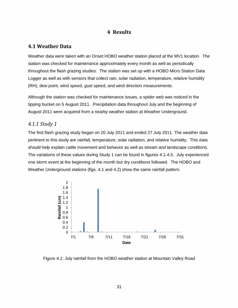
31

4 Results

4.1 Weather Data

Weather data were taken with an Onset HOBO weather station placed at the MV1 location. The

station was checked for maintenance approximately every month as well as periodically

throughout the flash grazing studies. The station was set up with a HOBO Micro Station Data

Logger as well as with sensors that collect rain, solar radiation, temperature, relative humidity

(RH), dew point, wind speed, gust speed, and wind direction measurements.

Although the station was checked for maintenance issues, a spider web was noticed in the

tipping bucket on 5 August 2011. Precipitation data throughout July and the beginning of

August 2011 were acquired from a nearby weather station at Weather Underground.

4.1.1 Study 1

The first flash grazing study began on 20 July 2011 and ended 27 July 2011. The weather data

pertinent to this study are rainfall, temperature, solar radiation, and relative humidity. This data

should help explain cattle movement and behavior as well as stream and landscape conditions.

The variations of these values during Study 1 can be found in figures 4.1-4.5. July experienced

one storm event at the beginning of the month but dry conditions followed. The HOBO and

Weather Underground stations (figs. 4.1 and 4.2) show the same rainfall pattern.

Figure 4.1: July rainfall from the HOBO weather station at Mountain Valley Road

0

0.2

0.4

0.6

0.8

1

1.2

1.4

1.6

1.8

2

7/1 7/6 7/11 7/16 7/21 7/26 7/31

Rain

fall

(c

m)

Date

32

Figure 4.2: July rainfall from KVAMCGAH2 station in McGaheysville, VA found through

Weather Underground

Figure 4.3: Temperature data, Study 1

0

0.5

1

1.5

2

2.5

7/1 7/6 7/11 7/16 7/21 7/26 7/31

Rain

fall

(c

m)

Date

15

20

25

30

35

40

7/19 7/21 7/23 7/25 7/27 7/29

Te

mp

era

ture

(oC

)

Date

33

Figure 4.4: Solar radiation data, Study 1

Figure 4.5: Relative humidity data, Study 1

4.1.2 Study 2

The second flash grazing study began on 15 August 2011 and stopped on 19 August 2011.

Figures 4.6-4.10 show the rainfall, temperature, relative humidity, and solar radiation for Study

2. There were many more rainfall events in August than in July 2011. There was a storm

before sampling started on 15 August 2011, but it did not affect stream flow or baseline levels

because rainfall amount were so small.

0

200

400

600

800

1000

1200

7/19 7/21 7/23 7/25 7/27 7/29

So

lar

rad

iati

on

(W

/m2)

Date

35

45

55

65

75

85

95

105

7/19 7/21 7/23 7/25 7/27 7/29

Rela

tive

hu

mid

ity (

%)

Date

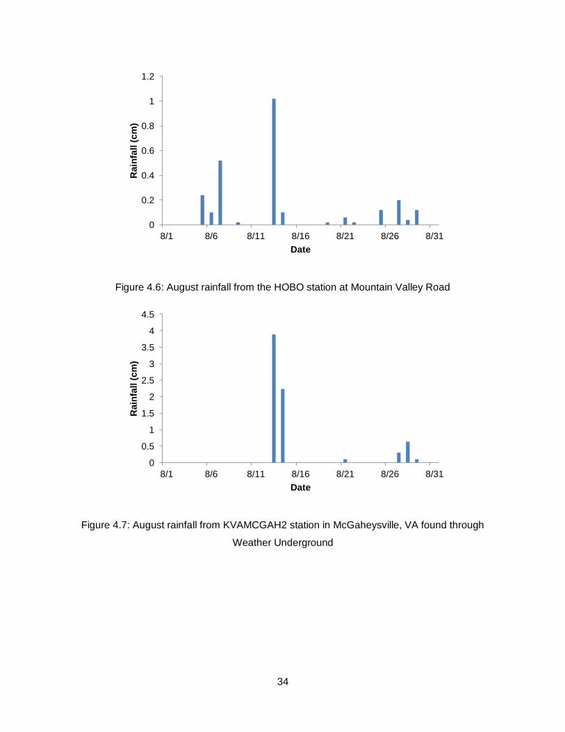
34

Figure 4.6: August rainfall from the HOBO station at Mountain Valley Road

Figure 4.7: August rainfall from KVAMCGAH2 station in McGaheysville, VA found through

Weather Underground

0

0.2

0.4

0.6

0.8

1

1.2

8/1 8/6 8/11 8/16 8/21 8/26 8/31

Rain

fall

(c

m)

Date

0

0.5

1

1.5

2

2.5

3

3.5

4

4.5

8/1 8/6 8/11 8/16 8/21 8/26 8/31

Rain

fall

(c

m)

Date

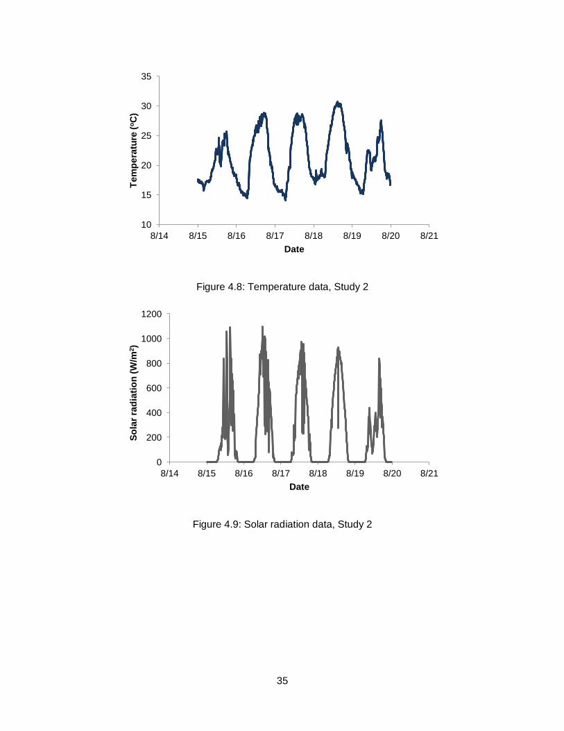
35

Figure 4.8: Temperature data, Study 2

Figure 4.9: Solar radiation data, Study 2

10

15

20

25

30

35

8/14 8/15 8/16 8/17 8/18 8/19 8/20 8/21

Te

mp

era

ture

(oC

)

Date

0

200

400

600

800

1000

1200

8/14 8/15 8/16 8/17 8/18 8/19 8/20 8/21

So

lar

rad

iati

on

(W

/m2)

Date

36

Figure 4.10: Relative humidity data, Study 2

4.2 Flow

Flow measurements were taken during each flash grazing study and figure 4.11 shows the flow

values taken at sites CR2, CR3, CM, MV1, and MV2 for dates 20 July 2011 and 19 August

2011. Because there was a 1.1cm rainfall event in two days before Study 2, flow was taken

before and after the study to ensure that the event did not affect baseflow conditions. Because

the flow rates on 16 August 2011 and 19 August 2011 were within a margin of error of 10%, the

rainfall that occurred prior was not considered to change baseflow conditions. By averaging

the flow measurements on 20 July, 16 August, and 19 August of the CR3 site, CR had a flow of

approximately 0.012 m3/s. Mountain Valley Road Tributary had a baseflow of approximately

0.007 m3/s by averaging the flow values from all three dates for stations MV1 and MV2. The

confluence of both the streams had a flow of approximately 0.022 m3/s at CM by averaging the

flow measurements on 20 July and 19 August.

40

50

60

70

80

90

100

110

8/14 8/15 8/16 8/17 8/18 8/19 8/20 8/21

Rela

tive

hu

mid

ity (

%)

Date

37

Figure 4.11: Flow by site and date

Along with flow measurements in figure 4.11, additional flow values were taken throughout the

2011 year and were compiled into a stage-discharge graphs (Appendix A). There are different

stage-discharge relationships for 2010 and 2011 due to a change in pressure transducer datum.

An exponential line of best-fit was determined, and the equation of that line was used to convert

ISCO levels from storm events into a representation of flow.

0

0.01

0.02

0.03

0.04

0.05

Flo

w (

m3/s

)

Site

39

4.3 Cattle Density and Pollutant Concentrations

To help determine the impact of cattle on water quality, the hunting cameras were used to track

cattle movement and behavior. The data from these cameras were downloaded and cattle were

counted and categorized as in-stream or in-fencing. Because there were no further flash

grazing studies in the literature review to help define cattle density, the following parameters

were calculated and compared:

Ave/Max # in stream

Ave/Max # in fencing

Ave/Max # in stream per stream length

Ave/Max # in fencing per riparian area

The stream parameter defines those cattle that were considered to be in the stream channel.

The fencing parameter defines the total number of cattle in the zone including those in the

stream and in the riparian area. The average and max values are based on two hour

increments to match the two hour water samples. These were then compared with the

corresponding bacteria and TSS times and concentrations to determine the best way to classify

cattle density.

First, the number and densities of cattle were compared with the downstream ISCO of each

zone. The camera data were then compared to the difference between the upstream and

downstream sites to account for any changes just in that particular zone. Once the

concentrations and densities were graphed against each other, a linear trendline was added

along with the corresponding coefficient of determination or R2 value. This was done for every

density parameter, and the one that had the greatest R2 value was chosen to be the most

correlated with the pollutant. Tables 4.1-4.6 show the best method and R2 value for each zone

for each study, and tables 4.5 and 4.6 show the combined data representing Studies 1 and 2

together.

40

Table 4.1: Cattle density method and R2 value for downstream and upstream-downstream zones compared with bacteria

concentrations, Study 1

Zone 1 Zone 2 Zone 3 Zone 4

Downstream Site Method[1] Max in fencing/area

(#/m2) Max in fencing

(#) Max in stream/length

(#/m) -

R2 [2] 0.54 0.105, (- slope) 0.309 -

Difference Upstream-Downstream

Method Ave in stream (#), per

length (#/m) Max in fencing

(#) Max in stream/length

(#/m) -

R2 0.37 0.106, (- slope) 0.307 -

[1] Cattle density method found in Appendix H that has the greatest R2 value as compared to bacteria [2] Coefficient of determination, R2, that has the greatest value based on a linear trendline comparing each density method and

bacteria concentrations

Table 4.2: Cattle density method and R2 value for downstream and upstream-downstream zones compared with bacteria



Downstream Site Method[1] Ave in fencing/area

(#/m2) Ave in stream (#), /area

(#/m2), and /length (#/m) Ave in fencing

(#) Max in fencing

(#)

R2[2] .0412, (- slope) 0.09 0.2124 0.1918


Method Ave in stream (#), per

length (#/m) Max in stream (#), /area

(#/m2), and /length (#/m) Ave in fencing

(#) Max in fencing

(#)

R2 0.238 0.518 0.2579 0.1055



41

Table 4.3: Cattle intensity method and R2 value for downstream and upstream-downstream zones compared with TSS



Downstream Site Method[1] Max in fencing/length

(#/m) Max in fencing

(#) Ave in stream/length

(#/m) -

R2 [2] 0.115 0.1378, (- slope)

0.851 -


Method Ave in stream (#) and

/length (#/m) Max in fencing

(#) Ave in fencing/area

(#/m2) -

R2 0.108 0.204, (- slope) 0.72 -

[1] Cattle density method found in Appendix H that has the greatest R2 value as compared to TSS [2] Coefficient of determination, R2, that has the greatest value based on a linear trendline comparing each density method and

TSS concentrations

Table 4.4: Cattle intensity method and R2 value for downstream and upstream-downstream zones for compared with TSS



Downstream Site Method[1] Ave in stream(#) and

/length (#/m) Ave in stream (#), /area

(#/m2), and /length (#/m) Ave in

fencing (#) Max in stream

(#)

R2 [2] 0.296 0.99 0.3998 0.27


Method Ave in stream (#) and

/length (#/m) Max in stream (#), /area

(#/m2), and /length (#/m) Ave in

fencing (#) Max in stream

(#)

R2 0.276 0.684 0.4545 0.265


TSS concentrations

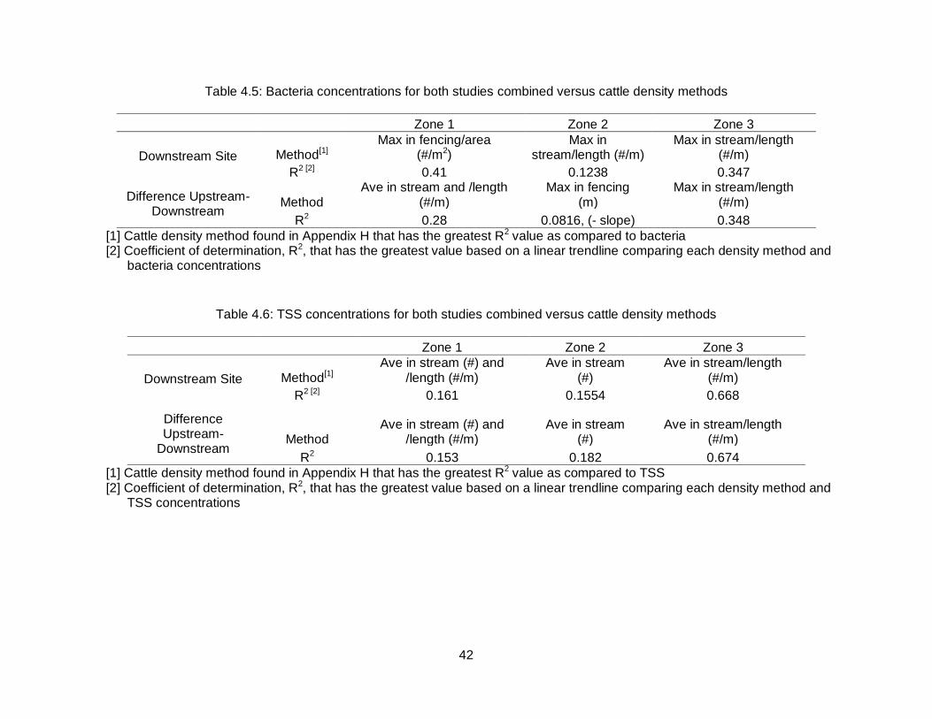
42

Table 4.5: Bacteria concentrations for both studies combined versus cattle density methods

Zone 1 Zone 2 Zone 3

Downstream Site Method[1] Max in fencing/area

(#/m2) Max in

stream/length (#/m) Max in stream/length

(#/m)

R2 [2] 0.41 0.1238 0.347


Method Ave in stream and /length

(#/m) Max in fencing

(m) Max in stream/length

(#/m)

R2 0.28 0.0816, (- slope) 0.348



Table 4.6: TSS concentrations for both studies combined versus cattle density methods


Downstream Site Method[1] Ave in stream (#) and

/length (#/m) Ave in stream

(#) Ave in stream/length

(#/m)

R2 [2] 0.161 0.1554 0.668

Difference Upstream-

Downstream Method

Ave in stream (#) and /length (#/m)

Ave in stream (#)

Ave in stream/length (#/m)

R2 0.153 0.182 0.674


TSS concentrations

43

The tables depict that there is not one method of best defining cattle densities. Some of the

methods are best correlated using averages, some with maximum values, some with the stream

counting, and some within fencing. The downstream and downstream – upstream sites have

approximate values for each method. Both of the studies have roughly the same R2 values for

each of the zones in tables 4.1 and 4.3 and tables 4.2 and 4.4. To look at both studies as a

whole, the time of cattle presence and pollutant concentrations were graphed using both Study

1 and Study 2 data. New methods and R2 values were calculated and found in tables 4.5 and

4.6. These tables depict that there are inconsistencies when determining a density method.

The combined zone 2 (table 4.5) has a negative slope for the difference from upstream to

downstream. This could be because Study 1 bacteria (table 4.1), although having an R2 of

approximately 0.082, the slope of the trendline is negative whereas the slopes on all the other

trendlines are positive. When combining this negative trendline values with the positive slope of

Study 2 (table 4.2), a negative R2 value is resulted as well. The negative slope could represent

too few cattle in the stream to account for any increases and the decreases would be due to the

natural flux of the water system. Also, when looking at the statistical charts in 4 Results –

Study 2 – Statistical Analysis – table 4.11 for zone 2 (CR2b-CR3), the bacteria concentration

statistically decreased representing that negative slope.

Along with the bacteria, TSS concentrations also show different fluxes in changes when

comparing the combined studies (table 4.6) with the separate ones (tables 4.3 and 4.4) –

sometimes the combined data set has a greater R2 and sometimes a smaller R2. Unlike the

bacteria for zone 2 with a negative slope, zone 2 TSS has a positive slope with an R2 of 0.155

(table 4.6) even though zone 2, Study 1 TSS has negative slopes (table 4.3). Zone 2, Study 1

TSS even has stronger R2 values than that of bacteria.

Also, although tables 4.5 and 4.6 show the greatest correlation between cattle densities and

bacteria and TSS concentrations, the R2 values are not very high. However, TSS does have

much stronger correlation values for most of the zones and studies, except zone 1. TSS is

expected to have higher correlation values because cattle stir up bed material by trampling but

do not necessary defecate in the stream.

The strongest R2 values overall can also be found at zone 3 or the CM site. The stronger

correlation at zone 3 could be due to the fact that this zone experienced much higher values

and increases than did the other zones. These higher values have a large influence on the

trendline and could make the R2 value appear to be more correlated. Although these higher

44

points may influence the trendline more, they also give a better representation of the cattle

influence on the stream.

For zone 2, cattle were found in the stream less often, and therefore had fewer two-hour periods

that cattle were in the stream or that zone. Zone 2 has very high R2 values for TSS in table 4.4

for Study 2, and this could be due to having just a few points that are very closely aligned.

Therefore, the R2 values are based off just a few points with possibly lower pollutant

concentration and cattle density values.

The influence of cattle on the TSS could also be partially due to the bed material of that site

being very mucky and free of cobble rocks that were present in upstream parts of Cub Run.

Cattle were seen in other parts of the stream; however, concentrations increased at a greater

rate in zone 3. A silty, mucky stream bed was much more mobile when disturbed versus a

stream bed full of rocks, cobbles, and debris.

45

4.4 Statistical Analysis

4.4.1 Study 1

In order to define period 2, the number of cattle in the stream and fencing areas were

determined using photographs from the hunting cameras. Period 2, or cattle influence, began

when two or more cattle were in the stream zone. However, if two or more cattle were found in

the stream of an upstream zone before a downstream zone, the downstream zone’s period 2

would begin at the time of the upstream zone’s period 2 starts. The start times for each of the

sites/zones can be found in table 4.7. Because zone four and five never had two or greater

cattle in the stream, there was no significant cattle influence to define period 2. Because

sampling for Study 1 had stopped on 24 July to conserve time and resources, the end of period

2 for all the zones is 24 July 4:00.

Table 4.7: Start and end dates and times for period 2 by zone, Study 1


Start 21 July 2011 18:00 21 July 2011 18:00 21July 2011 18:00

End 24 July 2011 4:00 24 July 2011 4:00 24 July 2011 4:00

In R statistics package, data sets were first tested for normality using a Shapiro test and found

to have a p-value less than alpha of 0.05, which indicates that the data sets are not normal. An

alpha of 0.05 was used for all the statistical tests because it is often used when analyzing

environmental data. The data was then natural log transformed and found to be normal. Under

the student’s t-test assumptions, the data must also have equal variance. Using a Bartlett test,

the data sets were found to not have equal variance.

Therefore, nonparametric tests were used to statistically analyze samples. A Wilcox test with a

Bonferroni correction was used to compare between periods for each station. Paired stations,

or upstream-to-downstream stations, were first compared using a Friedman’s test because it

has the most conservative p-value. The Friedman’s test compared the differences between the

four paired groups (CR1-CR2, CR2-CR2b, CR2b-CR3, FW-CM) along Cub Run. If the groups

were found to be different, a pairwise Wilcox test with a Bonferroni correction was used to

determine which pairs were dissimilar. The Bonferroni correction divides the p-value by the

number of samples and was used to maintain the error of making a false significance or Type I

error when performing multiple comparisons. Because there were only two pairs along MV,

simple paired Wilcox tests were used with the Bonferroni correction.

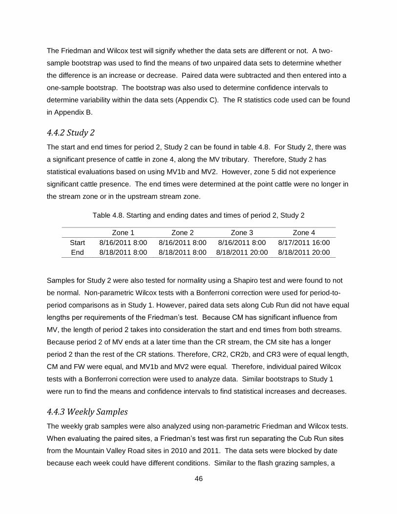
46

The Friedman and Wilcox test will signify whether the data sets are different or not. A two-

sample bootstrap was used to find the means of two unpaired data sets to determine whether

the difference is an increase or decrease. Paired data were subtracted and then entered into a

one-sample bootstrap. The bootstrap was also used to determine confidence intervals to

determine variability within the data sets (Appendix C). The R statistics code used can be found

in Appendix B.

4.4.2 Study 2

The start and end times for period 2, Study 2 can be found in table 4.8. For Study 2, there was

a significant presence of cattle in zone 4, along the MV tributary. Therefore, Study 2 has

statistical evaluations based on using MV1b and MV2. However, zone 5 did not experience

significant cattle presence. The end times were determined at the point cattle were no longer in

the stream zone or in the upstream stream zone.

Table 4.8. Starting and ending dates and times of period 2, Study 2


Start 8/16/2011 8:00 8/16/2011 8:00 8/16/2011 8:00 8/17/2011 16:00

End 8/18/2011 8:00 8/18/2011 8:00 8/18/2011 20:00 8/18/2011 20:00

Samples for Study 2 were also tested for normality using a Shapiro test and were found to not

be normal. Non-parametric Wilcox tests with a Bonferroni correction were used for period-to-

period comparisons as in Study 1. However, paired data sets along Cub Run did not have equal

lengths per requirements of the Friedman’s test. Because CM has significant influence from

MV, the length of period 2 takes into consideration the start and end times from both streams.

Because period 2 of MV ends at a later time than the CR stream, the CM site has a longer

period 2 than the rest of the CR stations. Therefore, CR2, CR2b, and CR3 were of equal length,

CM and FW were equal, and MV1b and MV2 were equal. Therefore, individual paired Wilcox

tests with a Bonferroni correction were used to analyze data. Similar bootstraps to Study 1

were run to find the means and confidence intervals to find statistical increases and decreases.

4.4.3 Weekly Samples

The weekly grab samples were also analyzed using non-parametric Friedman and Wilcox tests.

When evaluating the paired sites, a Friedman’s test was first run separating the Cub Run sites

from the Mountain Valley Road sites in 2010 and 2011. The data sets were blocked by date

because each week could have different conditions. Similar to the flash grazing samples, a

47

pairwise Wilcox test was used when weekly samples were found to be dissimilar. Paired data

was analyzed using paired Wilcox tests, and bootstraps were used to determine increases and

decreases between the two sets of data.

4.5 Study 1

4.5.1 Time Series Data

Samples were taken in two hour composites from 20 July 2011 to 27 July 2011. Sampling had

stopped at noon on 24 July and began again at noon on 25 July to conserve resources and

supplies. CR1 stopped sampling when cattle were first introduced to the riparian area also to

conserve time and resources.

The time series bacteria and TSS data for Cub Run during Study 1 can be seen in figures 4.12-

4.15. Points on the graph represent the beginning time of the two-hour sampling period. For

example, a point at 14:00 represents data from 14:00 – 15:45. CM was graphed with CR3 and

MV2 to show influence from each of the streams. Mountain Valley Road Tributary was not

graphed because cattle did not venture into this reach during the study. Because pH and EC

did not fluctuate throughout the study period, these parameters are not included in the analysis;

however, summary boxplots of the data are included in Appendix I.

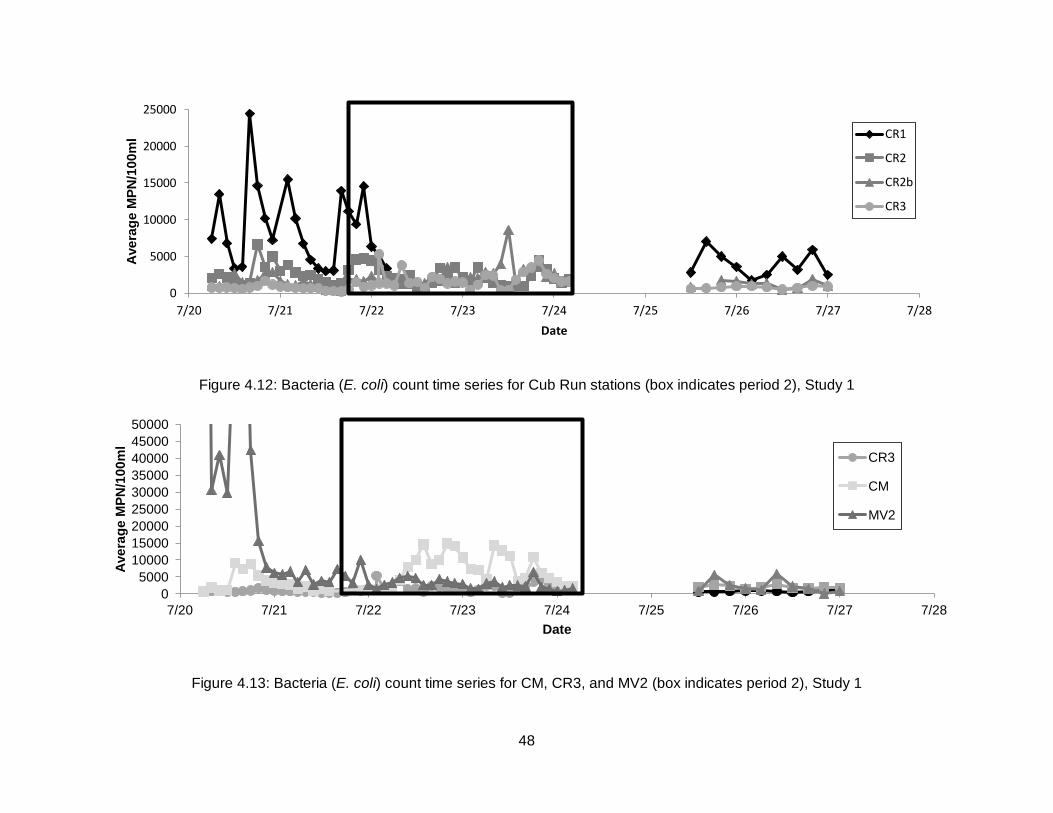
48

Figure 4.12: Bacteria (E. coli) count time series for Cub Run stations (box indicates period 2), Study 1

Figure 4.13: Bacteria (E. coli) count time series for CM, CR3, and MV2 (box indicates period 2), Study 1

0

5000

10000

15000

20000

25000

7/20 7/21 7/22 7/23 7/24 7/25 7/26 7/27 7/28

Ave

rag

e M

PN

/10

0m

l

Date

CR1

CR2

CR2b

CR3

0

5000

10000

15000

20000

25000

30000

35000

40000

45000

50000

7/20 7/21 7/22 7/23 7/24 7/25 7/26 7/27 7/28

Ave

rag

e M

PN

/10

0m

l

Date

CR3

CM

MV2

49

Figure 4.14: TSS time series for Cub Run sites (box indicates period 2), Study 1

Figure 4.15: TSS time series for CR3, CM, and MV2 (box indicates period 2), Study 1

0

20

40

60

80

100

120

140

7/20 7/21 7/22 7/23 7/24 7/25 7/26 7/27 7/28

TS

S (

mg

/L)

Date

CR1

CR2

CR2b

CR3

0

100

200

300

400

500

600

700

800

7/20 7/21 7/22 7/23 7/24 7/25 7/26 7/27 7/28

TS

S (

mg

/L)

Date

CR3

CM

MV2

50

In figure 4.12, the upstream influence from CR1 appears to vary considerably which is most

likely due to the free range cattle influence just upstream of this site. Because of this influence,

it is difficult to define a baseline concentration. Figure 4.12 also shows the general decrease in

bacteria concentrations in moving from upstream sites to downstream sites.

Figure 4.13 shows the influence that Mountain Valley Road Tributary has on the confluence site,

CM. Although the majority of the flow at the confluence is from Cub Run, MV noticeably

increased CM bacteria concentrations as seen at point 20 July 2011 14:00. However, when

cattle were allowed to graze within the riparian zone (period 2), the concentrations of CM

increased above those of MV2 and CR3 because of the additional cattle input.

Unlike the bacteria counts, the TSS concentrations of the upstream CR1 site does not appear to

have as much of an influence on TSS when looking comparing downstream sites (figs. 4.14 and

4.15). However, the concentrations are still variable, which also creates difficulty when defining

a baseline concentration. TSS concentrations also do not have the same pattern of decreasing

from upstream-to-downstream like the bacteria counts. Upstream cattle may have a greater

influence on bacteria concentrations than TSS through the CR reach.

4.5.2 Statistical Analysis

Period 1 was sampled before cattle were in the stream, and period 3 started when cattle exited

the stream riparian zone. Ideally, these two sets of samples should be equal because neither

period had cattle in the stream. If period 1 and 3 are not similar, any lingering influence of the

cattle may be seen in period 3. Looking at the statistical differences between periods 1 and 3 in

table 4.9, CR2b and FW (flow weight of MV2 and CR3) had the most significant increases and

decreases of all the sites. CR2b was found to have mostly increases from period 1 and 3 with a

decrease in TSS and equal bacteria concentrations. FW also had statistical increases in TSS

and PO4-P and a decrease in bacteria.

51

Table 4.9: Statistical comparisons of water quality parameters (concentrations) between no

cattle access periods 1 and 3 and baseline period 1 to cattle access period 2, Study 1.

Bacteria

(MPN/100ml) TSS

(mg/L) PO4-P (mg/L)

NO3-N (mg/L)

TP (mg/L)

TN (mg/L)

Pe

rio

d 1

, 3

CR2b =[2] ↑ ↓ ↑ ↑ ↑

CR3 = = = = = =

CM = = ↑ = = =

FW[1] ↓ ↑ ↑ = = =

Pe

rio

d 1

, 2

CR2 = ↓ = = = =

CR2b ↑ ↑ ↓ = ↑ ↑

CR3 ↑ ↑ = = ↑ =

CM ↑ ↑ ↑ = ↑ =

FW ↓ ↑ = = ↑ =

[1] FW = flow weight of MV2 and CR3 stations [2] Comparisons between periods were determined using non-parametric Wilcox tests to

determine whether the two data sets are equal or not equal by finding the differences by subtracting upstream from downstream. If statistically dissimilar, a two-sample bootstrap calculated means and confidence intervals on each data set to determine an increase or decrease.

Symbols in the table indicate the following: ↓ Statistical decrease from period 1 to 3 or period 1 to 2 ↑ Statistical increase from period 1 to 3 or period 1 to 2 = Statistically equal from period 1 to 3 or period 1 to 2 - No data

Statistically significant decrease from period 1 and 3 to period 1 and 2

Decrease in mean from period 1 and 3 to period 1 and 2

Statistically significant increase from period 1 and 3 to period 1 and 2

Mean increase from period 1 and 3 to period 1 and 2

When analyzing periods 1 and 2, CR2 shows roughly all statistically equal pollutants with the

exception of a decrease in TSS. This is to be expected because CR2 is the control sampling

station above the flash grazing cattle influence. However, CR2b, CR3, and CM show increases

from period 1 to period 2 in bacteria, TSS, and total phosphorous. FW also shows an increase

in TSS and total phosphorous but shows a decrease in bacteria concentrations. The decrease

in FW bacteria concentrations could be due to the decrease in concentrations of Mountain

Valley Road Tributary from period 1 to period 2.

52

By comparing periods 1 and 3 to periods 1 and 2, flash grazing cattle impacts can be seen. The

comparison between the two groups of periods can be seen in the shading scheme in table 4.9.

The lighter shades show when there was an increase in means comparing between periods 1

and 3 to periods 1 and 2 (and if it is statistically significant), and darker shades represent

decreases. When comparing period 1 to 2 in table 4.9, more statistical increases can be seen

than from period 1 to 3. The additional statistical increases are seen in bacteria, TSS, and TP.

Nitrogen concentrations did not change from baseline periods to the cattle access period. Most

of the deceases from period 1 and 3 to period 1 and 2 can be seen at the CR2b station.

Therefore, it is possible to infer that cattle increase bacteria, TSS, and TP concentrations at

most of the stations along Cub Run.

Table 4.10 shows the paired differences from upstream to downstream sites during the baseline

period 1 and the cattle influenced period 2. Pairing the sites by subtracting downstream -

upstream will eliminate input concentrations into each zone. The increases and decreases in

concentrations within each zone highlight cattle impacts within each zone. Finding the

differences in period 1 helps explain concentration fluxes in the stream without direct cattle

impact.

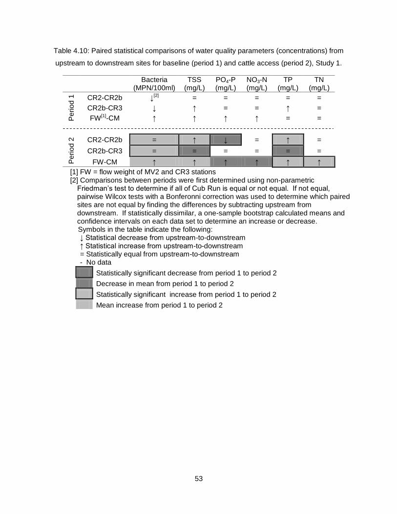
53

Table 4.10: Paired statistical comparisons of water quality parameters (concentrations) from

upstream to downstream sites for baseline (period 1) and cattle access (period 2), Study 1.

Bacteria

(MPN/100ml) TSS

(mg/L) PO4-P (mg/L)

NO3-N (mg/L)

TP (mg/L)

TN (mg/L)

Pe

rio

d 1

CR2-CR2b ↓[2] = = = = =

CR2b-CR3 ↓ ↑ = = ↑ =

FW[1]-CM ↑ ↑ ↑ ↑ = =

Pe

rio

d 2

CR2-CR2b = ↑ ↓ = ↑ =

CR2b-CR3 = = = = = =

FW-CM ↑ ↑ ↑ ↑ ↑ ↑

[1] FW = flow weight of MV2 and CR3 stations [2] Comparisons between periods were first determined using non-parametric

Friedman’s test to determine if all of Cub Run is equal or not equal. If not equal, pairwise Wilcox tests with a Bonferonni correction was used to determine which paired sites are not equal by finding the differences by subtracting upstream from downstream. If statistically dissimilar, a one-sample bootstrap calculated means and confidence intervals on each data set to determine an increase or decrease.

Symbols in the table indicate the following: ↓ Statistical decrease from upstream-to-downstream ↑ Statistical increase from upstream-to-downstream = Statistically equal from upstream-to-downstream - No data

Statistically significant decrease from period 1 to period 2

Decrease in mean from period 1 to period 2

Statistically significant increase from period 1 to period 2

Mean increase from period 1 to period 2

54

The majority of the statistical changes in all the pollutants in period 1 came from the flow

weighted FW and CM sites (table 4.10). The increases may explain that there are natural inputs

from the MV2 and CR3 sites to the CM site. Because the farmer had flash grazed many times

before this study, the previous influence of cattle may explain the increases in pollutant

concentrations with previously placed fecal piles and stream bank impacts within that zone. For

period 2, FW – CM also saw all increases in concentrations. However, the mean difference for

period 1 is 2,903 MPN/100ml where the mean difference for period 2 is 6,945 MPN/100ml which

is greater than a 2 times increase. These means can also be found in Appendix C. Therefore,

although bacteria concentrations increased in times of no direct cattle influence from FW to CM,

concentrations increased much more in times of cattle influence.

Decreases in bacteria concentrations in period 1 from CR2 – CR2b and CR2b – CR3 sites may

be due to attenuation downstream from the upstream free cattle access influence. Contrary to

results from the FW-CM sites, CR2-CR2b showed varying results and CR2b-CR3 had no

statistical change in any of the pollutants during period 2. The two pairs also showed increases

and decreases from period 1 to period 2. Thus, an impact from cattle is not significant within

zone 1 and 2 from CR2 to CR3.

Overall, table 4.10 illustrates that cattle impacts are variable except in zone 3 from FW to CM.

Similarly with Study 1, the majority of increases from period 1 to period 2 were seen in bacteria,

TSS, and TP concentrations. Also, NO3-N and TN had little change between periods and sites.

55

4.6 Study 2

4.6.1 Time Series Data

Samples were collected from 15 August 2011 to 19 August 2011. Figures 4.16 – 4.21 show the

time lapse data split between CR, CM and upstream sites, and MV. Mountain Valley Road

Tributary graph was included in Study 2 because there was a significant presence of cattle.

Along with Study 1, Study 2 did not show any changes through the different periods for pH or

EC; therefore, boxplots of this data can be found in Appendix I. Also for Study 2, CR1 was

sampled during the entire study period to capture effects from the upstream cattle.

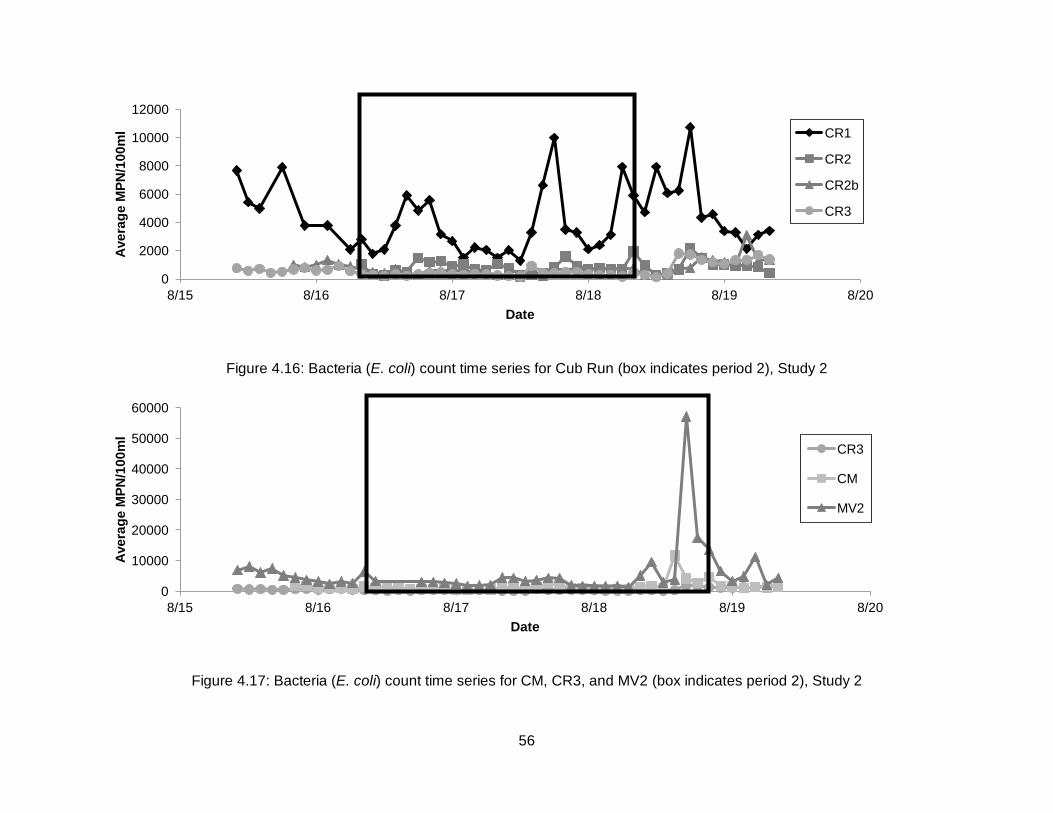
56

Figure 4.16: Bacteria (E. coli) count time series for Cub Run (box indicates period 2), Study 2

Figure 4.17: Bacteria (E. coli) count time series for CM, CR3, and MV2 (box indicates period 2), Study 2

0

2000

4000

6000

8000

10000

12000

8/15 8/16 8/17 8/18 8/19 8/20

Ave

rag

e M

PN

/10

0m

l

Date

CR1

CR2

CR2b

CR3

0

10000

20000

30000

40000

50000

60000

8/15 8/16 8/17 8/18 8/19 8/20

Ave

rag

e M

PN

/10

0m

l

Date

CR3

CM

MV2

57

Figure 4.18: Bacteria (E. coli) count time series for Mountain Valley Road Tributary (box indicates period 2), Study 2

Figure 4.19: TSS time series for Cub Run (box indicates period 2), Study 2

0

10000

20000

30000

40000

50000

60000

8/15 8/16 8/17 8/18 8/19 8/20

Ave

rag

e M

PN

/10

0m

l

Date

MV1

MV1b

MV2

0

50

100

150

200

250

300

8/15 8/16 8/17 8/18 8/19 8/20

TS

S (

mg

/L)

Date

CR1

CR2

CR2b

CR3

58

Figure 4.20: TSS time series for CM, CR3, and MV2 (box indicates period 2), Study 2

Figure 4.21: TSS time series for Mountain Valley Road Tributary (box indicates period 2), Study 2

0

500

1000

1500

2000

2500

3000

3500

4000

8/15 8/16 8/17 8/18 8/19 8/20

TS

S (

mg

/L)

Date

CR3

CM

MV2

0

500

1000

1500

2000

2500

3000

3500

4000

8/15 8/16 8/17 8/18 8/19 8/20

TS

S (

mg

/L)

Date

MV1

MV1b

MV2

59

Study 2 also shows fluctuating bacteria concentrations at CR1 in figure 4.16. The increases

come during late afternoon, which is consistent with the times that cattle are in the stream found

in Appendix H. Fluctuating concentrations makes baseline levels very difficult to determine.

Figure 4.16 also shows that bacteria concentrations decrease rapidly downstream of the cattle

site, and concentrations continue to decrease further downstream as well. Therefore, these

decreases in bacteria conventions makes finding a baseline level for the downstream Cub Run

sites more feasible. CM also does not show many fluctuations, which is due to upstream

streams not having large fluctuations. Figure 4.18 also shows a large fluctuation at MV1, just

downstream of free range cattle. Just like Cub Run, bacteria counts attenuate downstream

creating more consistent concentrations to MV1b and MV2.

For TSS, figures 4.19-4.21 appear to have steady, baseline levels of sediment. Even the

upstream sites of CR1 and MV1 do not have the fluctuations like those seen in the bacteria

graphs. Therefore, baseline levels of sediment are much easier to define. The peaks in period

2 in figures 4.19-4.21may be due to flash grazing cattle influence.

4.6.2 Statistical Analysis

Table 4.11 shows the statistical results between the flash grazing periods. Periods 1 and 3

were compared to look at differences between the non-cattle influenced periods. Periods 1 and

2 were compared to look at any changes from pre-cattle influence to during cattle influence time

frames. When comparing periods 1 and 3 for all the sites and all the pollutants, very little

changes can be seen. There was only one change in nutrients found in NO3-N at MV2. The

majority of the changes, which were increases, are found in TSS concentrations of various sites

in the study area.

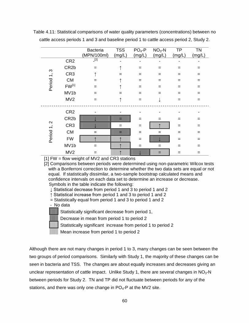
60

Table 4.11: Statistical comparisons of water quality parameters (concentrations) between no

cattle access periods 1 and 3 and baseline period 1 to cattle access period 2, Study 2.

Bacteria (MPN/100ml)

TSS (mg/L)

PO4-P (mg/L)

NO3-N (mg/L)

TP (mg/L)

TN (mg/L)

Pe

rio

d 1

, 3

CR2 -[2] - - - - -

CR2b = ↑ = = = =

CR3 ↑ = = = = =

CM = ↑ = = = =

FW[1] = ↑ = = = =

MV1b = = = = = =

MV2 = ↑ = ↓ = =

Pe

rio

d 1

, 2

CR2 - - - - - -

CR2b ↓ = = = = =

CR3 ↓ = = ↑ = =

CM = = = = = =

FW ↑ ↑ = ↓ = =

MV1b = ↑ = = = =

MV2 = ↑ ↓ = = =

[1] FW = flow weight of MV2 and CR3 stations [2] Comparisons between periods were determined using non-parametric Wilcox tests

with a Bonferroni correction to determine whether the two data sets are equal or not equal. If statistically dissimilar, a two-sample bootstrap calculated means and confidence intervals on each data set to determine an increase or decrease.

Symbols in the table indicate the following: ↓ Statistical decrease from period 1 and 3 to period 1 and 2 ↑ Statistical increase from period 1 and 3 to period 1 and 2 = Statistically equal from period 1 and 3 to period 1 and 2 - No data

Statistically significant decrease from period 1,




Although there are not many changes in period 1 to 3, many changes can be seen between the

two groups of period comparisons. Similarly with Study 1, the majority of these changes can be

seen in bacteria and TSS. The changes are about equally increases and decreases giving an

unclear representation of cattle impact. Unlike Study 1, there are several changes in NO3-N

between periods for Study 2. TN and TP did not fluctuate between periods for any of the

stations, and there was only one change in PO4-P at the MV2 site.

61

Reviewing table 4.11 shows that TP and TN did not statistically change except between FW to

CM in period 2. Another point of interest is that PO4 did not change at all except when

comparing MV2 period 1 and 2 and the same CM to FW in period 2. Therefore, in general,

nutrients did not change much from period-to-period and upstream-to-downstream.

Table 4.12 shows the differences between paired sites for period 1 and period 2. Similar to

table 4.11, there are not many changes in pollutant concentrations in the paired sites with the

only changes in bacteria and TSS. With all of the paired sites, only period 2 FW-CM showed

increases in nutrient concentrations.

Table 4.12: Paired statistical comparisons of water quality parameters (concentrations) from

upstream to downstream sites for baseline (period 1) and cattle access (period 2), Study 2.

Bacteria

(MPN/100ml) TSS

(mg/L) PO4-P (mg/L)

NO3-N (mg/L)

TP (mg/L)

TN (mg/L)

Pe

rio

d 1

CR2-CR2b -[2] - - - - -

CR2b-CR3 ↓ = = = = =

FW[1]-CM ↑ ↑ = = = =

MV1b-MV2 = ↑ = = = =

Pe

rio

d 2

CR2-CR2b ↓ = = = = =

CR2b-CR3 ↓ = = = = =

FW-CM ↑ ↑ ↑ ↑ ↑ ↑

MV1b-MV2 = ↑ = = = =

[1] FW = flow weight of MV2 and CR3 stations [2] Comparisons between periods were determined using non-parametric Wilcox tests to

determine whether the two data sets are equal or not equal by finding the differences by subtracting upstream from downstream. If statistically dissimilar, a one-sample bootstrap calculated means and confidence intervals on each data set to determine an increase or decrease.

Symbols in the table indicate the following: ↓ Statistical decrease from upstream-to-downstream ↑ Statistical increase from upstream-to-downstream = Statistically equal from upstream-to-downstream - No data

Statistically significant decrease from period 1 to period 2




62

Another point of interest is that FW-CM increased in every pollutant from period 1 to 2. An

increase can be seen in period 1 for bacteria and TSS; however, the mean difference for

bacteria in period 1 is 1,250 and the mean difference for period 2 is 1,695 MPN/100ml. For

TSS, period 1 has a mean difference of 7.3 mg/L for period 1 and 18.4 mg/L for period 2 also

suggesting that cattle have the potential to increase sediment concentrations. The CM and FW

sites are the only sites that show a statistical increase from period 1 to period 2 with the

exception of MV1b-MV2 TSS. Because FW-CM was the only sites to experiences significant

increases, flash grazing cattle do not appear to influence any of the other sites.

63

4.7 Return to Baseline Concentrations

The time it takes for concentrations to return to baseline concentrations is important to

understand when trying to characterize the intensity of an event as well as how the system

interacts with pollutants. It also helps quantify the impact of a flash grazing event. As seen in

the time series graphs for both studies (figs. 4.12-4.21), CR1 and MV1 have bacteria

concentrations that are variable, and most of the peaks can be seen during the afternoon when

cattle are more likely to be in the stream zone due to hotter temperatures. The lowest values

found in the fluctuations may not be baseline concentrations due to bacteria still in the system

from cattle presence. Determining the time it takes for pollutants to return to baseline can help

characterize whether the system can fully recover before a new event the next day. If

concentrations never return to a baseline level, then there is a continuing input of bacteria into

the system, and cattle have a lasting effect beyond the immediate disturbance.

To determine a baseline level for TSS, period 1 concentrations were averaged. However,

bacteria concentrations were quite variable and often did not have a clear baseline because of

the prominent upstream influence. Therefore, upstream samples were subtracted from

downstream sites to determine a difference in concentrations. Pairing data sets may provide a

steadier level by subtracting out upstream influence. However, this is not the case, and

concentrations were still quite inconsistent. When determining the time of peak impact, the

peak latest in time was used. The lated peak in period 2 is used because no other inputs

should be affecting concentrations. The date and time of this peak is then recorded. Cattle did

not always have a defined peak though such as zone 2 or CR3 – CR2b for study 1. When

concentrations did not appear to change from baseline, there was no need to define a baseline.

When concentrations reached the baseline concentrations after the peak, the date and time

were noted. The number of hours between the peak and the baseline concentrations were

found by subtracting the peak time and the time at which the concentration returned to baseline.

However, many of these concentrations, as seen in tables 4.13 and 4.14, do not return to

baseline levels because sampling had stopped too soon. Therefore, the percent recovery was

calculated instead, and these values are very close to being fully recovered. Because the

percent recoveries were very high, the time it takes these concentrations to return to baseline

are parallel with the times it took for fully recovered concentrations to return to baseline.

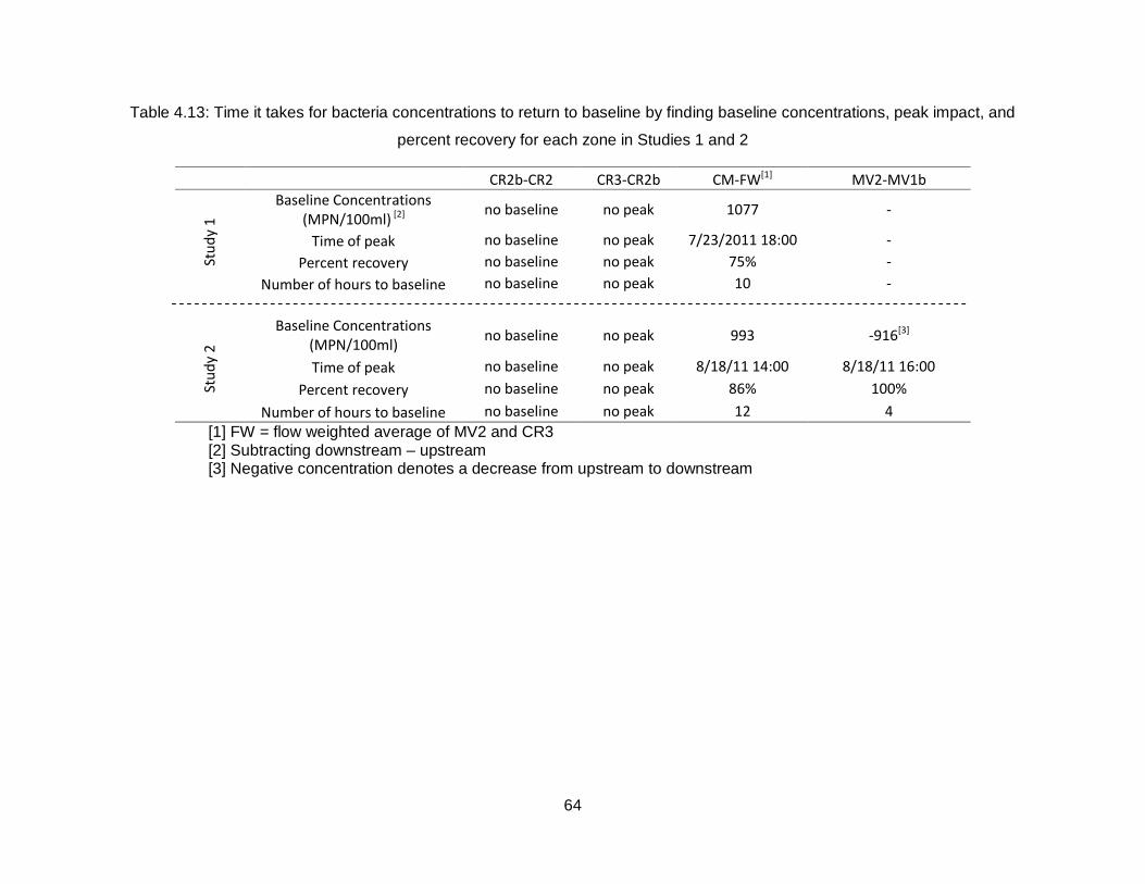
64

Table 4.13: Time it takes for bacteria concentrations to return to baseline by finding baseline concentrations, peak impact, and

percent recovery for each zone in Studies 1 and 2

CR2b-CR2 CR3-CR2b CM-FW[1] MV2-MV1b

Stu

dy

1

Baseline Concentrations (MPN/100ml) [2]

no baseline no peak 1077 -

Time of peak no baseline no peak 7/23/2011 18:00 -

Percent recovery no baseline no peak 75% -

Number of hours to baseline no baseline no peak 10 -

Stu

dy

2

Baseline Concentrations (MPN/100ml)

no baseline no peak 993 -916[3]

Time of peak no baseline no peak 8/18/11 14:00 8/18/11 16:00

Percent recovery no baseline no peak 86% 100%

Number of hours to baseline no baseline no peak 12 4

[1] FW = flow weighted average of MV2 and CR3 [2] Subtracting downstream – upstream [3] Negative concentration denotes a decrease from upstream to downstream

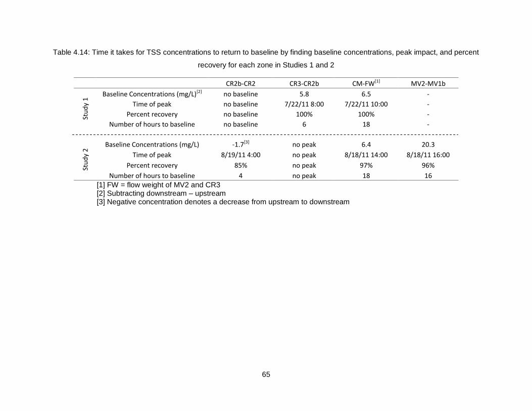
65

Table 4.14: Time it takes for TSS concentrations to return to baseline by finding baseline concentrations, peak impact, and percent

recovery for each zone in Studies 1 and 2

CR2b-CR2 CR3-CR2b CM-FW[1] MV2-MV1b St

ud

y 1

Baseline Concentrations (mg/L)[2] no baseline 5.8 6.5 -

Time of peak no baseline 7/22/11 8:00 7/22/11 10:00 -

Percent recovery no baseline 100% 100% -

Number of hours to baseline no baseline 6 18 -

Stu

dy

2 Baseline Concentrations (mg/L) -1.7[3] no peak 6.4 20.3

Time of peak 8/19/11 4:00 no peak 8/18/11 14:00 8/18/11 16:00

Percent recovery 85% no peak 97% 96%

Number of hours to baseline 4 no peak 18 16

[1] FW = flow weight of MV2 and CR3 [2] Subtracting downstream – upstream [3] Negative concentration denotes a decrease from upstream to downstream

66

Zone 3 (CM- FW) generally had the longest times to return to baseline, which could be due to

having greater peak impacts than other sites such as zones 1 and 2. Zone 4 (MV2-MV1b) had

a quick return in bacteria levels (4 hrs), with a longer time taken for TSS concentrations to return

to baseline conditions (16 hrs). TSS concentrations also appeared to have more peak impacts

in the zones, which could be due to steadier baseline concentrations. Impacts are more readily

seen when there are steadier baseline levels as with TSS versus bacteria concentrations.

4.8 Turbidity as an Indicator of Impact

Analyzing concentrations of pollutants takes an extensive amount of time and resources such

as access to a laboratory. The general public does not have access to such equipment and

time. Because turbidity can be easily seen, it could make a useful measure of impact. There is

no special equipment or needs associated with looking at the stream and determining how

turbid or cloudy it is. Although the exact concentration of the stream would not be easy to

determine, relative levels can be seen. In contrast, visual observations are not useful when

determining different levels of bacteria or nutrients, for example.

Figures 4.22-4.25 show the time series turbidity data for Cub Run and CM with corresponding

upstream sites for Study 1 and CM with corresponding upstream sites and Mountain Valley

Road Tributary for Study 2. Not all graphs and sites are included because the only sites with

peaks are zone 2 and 3 for Study 1 and zone 3 and 4 for Study 2. The other sites have fairly

constant baseline turbidity levels throughout the whole study. Because there was no significant

cattle influence in zone 4 during Study 1, the increase in turbidity at MV2 in figure 4.23 is likely

due to upstream conditions and not flash grazing activity.

68

Figure 4.22: Turbidity time series for Cub Run (box indicates period 2), Study 1

Figure 4.23: Turbidity time series for CM, CR3, and MV2 (box indicates period 2), Study 1

0

50

100

150

200

7/20 7/21 7/22 7/23 7/24 7/25 7/26 7/27 7/28

Tu

rbid

ity (

NT

U)

Date

CR1

CR2

CR2b

CR3

0

50

100

150

200

7/20 7/21 7/22 7/23 7/24 7/25 7/26 7/27 7/28

Turb

idit

y (N

TU)

Date

CR3

CM

MV2

69

Figure 4.24: Turbidity time series for CM, CR3, and MV2 (box indicates period 2), Study 2

Figure 4.25: Turbidity time series for MV (box indicates period 2), Study 2

0

200

400

600

800

1000

8/15/11 8/16/11 8/17/11 8/18/11 8/19/11 8/20/11

Tu

rbid

ity (

NT

U)

Date

CR3

CM

MV2

0

200

400

600

800

1000

8/15/11 8/16/11 8/17/11 8/18/11 8/19/11 8/20/11

Tu

rbid

ity (

NT

U)

Date

MV1

MV1b

MV2

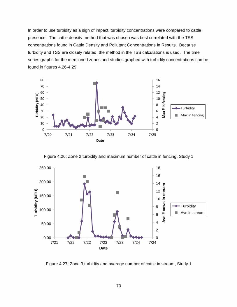
70

In order to use turbidity as a sign of impact, turbidity concentrations were compared to cattle

presence. The cattle density method that was chosen was best correlated with the TSS

concentrations found in Cattle Density and Pollutant Concentrations in Results. Because

turbidity and TSS are closely related, the method in the TSS calculations is used. The time

series graphs for the mentioned zones and studies graphed with turbidity concentrations can be

found in figures 4.26-4.29.

Figure 4.26: Zone 2 turbidity and maximum number of cattle in fencing, Study 1

Figure 4.27: Zone 3 turbidity and average number of cattle in stream, Study 1

0

2

4

6

8

10

12

14

16

0

10

20

30

40

50

60

70

80

7/20 7/21 7/22 7/23 7/24 7/25

Max

# in

fen

cin

g

Turb

idit

y (N

TU)

Date

Turbidity

Max in fencing

0

2

4

6

8

10

12

14

16

18

0.00

50.00

100.00

150.00

200.00

250.00

7/21 7/22 7/22 7/23 7/23 7/24 7/24

Ave

# c

ow

s in

ste

ram

Tu

rbid

ity (

NT

U)

Date

Turbidity

Ave in stream

71

Figure 4.28: Zone 3 turbidity and average number of cattle in fencing, Study 2

Figure 4.29: Zone 4 turbidity and maximum number of cattle in stream, Study 2

As seen in the figures 4.26-4.29, there was a consistent pattern that when there were cattle in

the stream or fencing, concentrations increased. It also appears that when the cattle density

reaches approximately three in stream or in fencing, concentrations tend to increase.

Note that just because cattle went above the three cattle approximation, does not mean that

turbidity concentrations increased as seen in figure 4.29. The density methods mentioned were

0

1

2

3

4

5

6

7

0

20

40

60

80

100

120

8/17 8/17 8/18 8/18 8/19 8/19

Ave

in f

enci

ng

Turb

idit

y (N

TU)

Date

Turbidity

Ave in fencing

0

0.5

1

1.5

2

2.5

3

3.5

4

4.5

0

100

200

300

400

500

600

700

800

900

8/14 8/15 8/16 8/17 8/18 8/19 8/20

Max

# in

str

eam

Turb

idit

y (N

TU)

Date

Turbidity

Max in stream

72

also the density method with the greatest correlation, and the correlations were not highly

significant with low R2 values. There may have been more cattle present that were not

represented in these density methods.

However, in figure 4.27, the relationship between cattle and turbidity were very close. Figure

4.27 represented zone 3, which also had the highest R2 relationships for bacteria and TSS. The

high correlation could be because the bed material of this zone was more mobile and increases

at smaller amounts of cattle movement.

Once a level of turbidity was established, it will be important to educate the public that looking at

the stream at one point of time is not necessarily representative of an event. A stream might

naturally be cloudy at baseline levels, so seeing it at one point in time does not necessarily

mean that there are cattle present. There are many reasons that a stream may have high

turbidity, and cattle are just one possible cause.

4.9 Storm Concentrations

Storm samples were also collected as part of this research study. In order to compare the

intensity of cattle influence on water quality, the loads from the flash studies were compared

with those of several storms. Ten storms throughout 2010 and 2011 were sampled. The

storms chosen to compare with the flash grazing study were storms III, V, IX, and X. These

were chosen because they had clear baselines and peaks. MV2 was also chosen as the site to

compare concentrations because only the permanent ISCOs take storm samples. MV1 and

CR1 are upstream of the flash grazing, and CM is not in place during storm events. Therefore,

MV2 and CR3 are remaining, and CR3 does not have any clear peak impacts due to cattle

presence in the flash grazing study. During Study 2, MV2 has a clear peak in TSS but not in

any other pollutant. Thus, only TSS can be compared because all of the other water quality

parameters do not show increases above a baseline level. The graphs of the chosen storms

with TSS and flow can be found in Appendix D. Also, several characteristics of the storms are

shown in table 4.15.

73

Table 4.15: Storm dates, intensities, rainfall amounts, and duration

Event Date Rainfall (in) Duration (hr) Intensity (in/hr)

Storm III 7/13/10-7/14/10 1.79 22 0.08

Storm V 9/30/10-10/1/10 2.59 23 0.11

Storm IX 9/5/11-9/6/11 1.62 14 0.12

Storm X 10/12/2011 0.90 15 0.06

Note that the rainfall amounts for storms V and X came from sister stations on Silver Creek

(SL3) near Singers Glen, Virginia due to lack of data at the Mountain Valley Road weather

station.

Because the comparison is based on loads, the first step was to define a baseline level so only

the peaks can be counted for total load. For the flash grazing study, the baseline was relatively

easy to define because the concentrations have been consistently level throughout the study.

The stable concentrations were then averaged to determine a baseline level. The start of the

peak was clearly defined from the time series graph of the data. After the peak, when

concentrations returned to the baseline levels, calculations stopped. However, not all

concentrations returned to a baseline level after the peak, so loads can only be based on the

collected data, thus not counting the total load of the event.

Storm loads were figured the same way by selecting a baseline concentrations and taking the

load on everything above baseline. With the storms, few samples were collected, and it was

more difficult to create a baseline. For all of the graphs, there are no two or more points before

the maximum value that is stable enough to be considered baseline. Therefore, loads started

for each storm at the first sample. Also, the graphs show that there are few to no points that

level off after the peak values, so for storms III, V, and X, all of the samples were used to create

a load. Storm IX load was calculated from the beginning until 6 September 11 8:30 because

after this point there was a break in the samples until 6 September 11 15:30. The

concentrations from this point onward in time appear to be at a steady level as well.

Using the corresponding year stage-discharge graphs, the level recorded by the ISCO was

converted to flow. Because level was taken every five minutes, it was averaged over the same

time period that samples were collected. For example, if the ISCO was programmed to take

one hour composites in each bottle, the corresponding levels within that hour were averaged to

find one volume. Then, total load was calculated as follows:

74

(2)

The loads for each bottle were then summed and converted to kilograms. Table 4.16 shows the

total loads and percentages for each storm and the flash grazing event during Study 2.

Table 4.16 Storm and flash grazing Study 2 TSS loads and percentage of storm load compared

to flash grazing Study 2 load

Event TSS (kg) (kg/hour) Storm Load as % of Study 2

Storm III 863 39 289%

Storm V 3497 152 1170%

Storm IX 336 24 112%

Storm X 286 19 96%

Study 2 299 17 -

Table 4.16 also shows the load per hour to normalize all the events. Normalizing the events did

not change the results greatly as Storm IX and X have comparable loads to the flash grazing

event. Storm III’s total load is about three times greater than the flash grazing event, but the

normalizing makes it about twice as large as the Study 2 load. Storm V for the total load and

normalized load has a much greater load than the flash grazing event at approximately 12 times

greater.

In conclusion, Storms IX and X have comparable loads to that of a flash grazing event and

storms III and V has much higher loads. Although the storms have approximately equal

intensities, the rainfall amounts vary. Storm V with over 2.5 inches of rain had the greatest

impact on load and showed an 1170% increase over the flash grazing study.

4.10 Weekly Grab Samples

The weekly grab samples collected during the spring, summer, and fall of 2010 and 2011 were

used to compare changes in stream concentrations over these two summer seasons. During

the fall of 2010, cattle were introduced to the pasture immediately upstream of CR1a where the

cattle had free access to the stream. The pasture upstream of CR1a had no stream fencing and

the stream in the pasture was the primary water source for the cattle. This change in land use

is important to note when comparing pollutant concentrations between years.

Each site was evaluated comparing years as well as pairing upstream and downstream

concentrations for each year. Each comparison was run for nutrients NH4-N, PO4-P, NO3-N,

75

total nitrogen (TN), total phosphorus (TP), turbidity, TSS, E.coli bacteria counts, pH, and

electrical conductivity (EC) in table 4.17. Little significant change in concentration of pH, EC,

TN, and NO3-N were found and can be seen in Appendix J.

76

Table 4.17: Statistical comparisons of water quality parameters (concentrations) of weekly grab samples from 2010 to 2011 and

paired sites in 2010 and 2011

Bacteria

(MPN/100ml) TSS

(mg/L) Turbidity (NTU) pH

EC (μS)

NH3-N (mg/L)

PO4-N (mg/L)

NO3-N (mg/L)

TN (mg/L)

TP (mg/L)

20

10

-201

1

CR1a[2] ↑[1] ↑ ↑ = ↓ - = = = =

CR1b ↑ = ↑ = ↓ - = = = =

CR2 ↑ = = = ↓ - = = = =

CR3 ↑ = = = ↓ - = = = =

MV1 = ↑ ↑ = = - ↑ ↓ ↑ =

MV2 = ↑ ↑ = = - ↓ ↓ ↑ =

20

10

CR1a-CR1b = = = = = = = = = ↑

CR1b-CR2 = = = = = ↓ ↓ = = =

CR2-CR3 = = = = = = ↓ = = ↓

MV1-MV2 = = ↓ = = ↓ = = = ↓

20

11

CR1a-CR1b = = = = = - = = = =

CR1b-CR2 ↓ = = = = - = = = =

CR2-CR3 = = = = = - = = = =

MV1-MV2 ↓ = ↓ = = - = = = =

[1] Statistical significance between 2010 and 2011 was found running a non-parametric Wilcox test with a Bonferroni correction. If 2010 and 2011 were found to be statistically dissimilar, a two-sample bootstrap was run to determine means and confidence intervals to determine increases and decreases. The last two groups of rows were found first using a non-parametric Friedman’s test to determine significance among all the sites on Cub Run. If dissimilar, a pairwise Wilcox test with a Bonferroni correction was run to determine which pairs are not equal. A one-sample bootstrap was run using downstream minus upstream data.

Symbols in the table indicate the following: ↓ Statistical decrease from either 2010 to 2011 or upstream-to-downstream ↑ Statistical increase from either 2010 to 2011 or upstream-to-downstream = Statistically equal from 2010 to 2011 or upstream-to-downstream - No data [2] CR1a is just upstream of the CR1 bridge; CR1b is same as flash grazing CR1

77

When comparing the 2010 to 2011 data, there is a significant increase in bacteria

concentrations for all of the Cub Run sites. The increase could be due to the introduction of

cattle upstream of CR1a in the last fall of 2010 and show that cattle have a significant influence

on stream water quality within one season. Bacteria, unlike TSS and turbidity, show increases

downstream as well. The mean differences from 2010 to 2011by subtracting upstream from

downstream for the Cub Run sites are as follows in order of upstream to downstream: -3321, -

6001, -1127, and -1174 MPN/100ml respectively. A negative mean difference indicates that

downstream is greater than upstream. The increase in TSS and turbidity at CR1a could also be

due to upstream cattle. Downstream sites may not show an increase due to settling.

The Cub Run sites also show a significant decrease in electrical conductivity from 2010 to 2011,

which most likely cannot be explained from the introduction of cattle. In the literature review,

cattle have been found to have little to no effect on the salinity of water. Cattle can, however,

stir up bed material and rock that may have captured settled salts thus creating an increase in

salinity and electrical conductivity.

Table 4.17 also shows that both MV sites have increases in TSS, turbidity, and TN in 2011.

Mountain Valley Road tributary also had a strong cattle presence upstream that could contribute

to the increase in sediment. However, the increase in bacteria did not change, but through the

cutting back of banks and storm events, sediment could have become unsettled even when

cattle were not present in the stream. The silty, mucky streambed of MV is mobile and can be

suspended into the water column easily. The increase in total nitrogen may be from natural

sources as the literature review notes that cattle have little influence on nitrogen concentrations.

Although both these sites had increases in total nitrogen, both sites, however, had a decrease in

NO3-N and equal amounts of NH3-N; therefore, there may have been sampling/laboratory error

or another source of nitrogen causing the increase.

The last two groups of rows looks at the paired differences from upstream-to-downstream to

determine what was occurring throughout the stream reach. In 2010, there were few changes

except for nutrient decreases. The nutrient decreases do not show patterns in pollutants or

sites. While 2010 had only changes in nutrients, 2011 had no significant changes except in

bacteria and turbidity. The differences were found in sites that were closest to the upstream

cattle influence. Although the free access cattle upstream of the study site may have

contributed to the increases in concentrations at the upstream stations, the free access cattle

78

upstream may not have significant influence on concentrations of stations further downstream of

the immediate influence.

When analyzing the paired data sets for 2010 and 2011 there are no significant differences

between the CREP zone (CR1-CR2) and the flash grazing zones (CR2-CR3). Although there

were noticeable increases during the immediate impact of cattle, there were no noticeable long-

term impacts of flash grazing when analyzing weekly grab samples.

The only common significance for the MV tributary for both years was the decrease in turbidity

from MV1 to MV2. The cattle influence upstream of MV1 was present during both years, and

there were no major changes upstream on MV. The decrease in turbidity from MV1 to MV2

could largely be due to stream characteristics. MV1 was also placed in a stream bend that was

consistently covered by sediment due to deposition whereas while MV2 was downstream of a

straight reach segment lined with tall grasses.

4.11 Effects of CREP Zone

Although this project focuses on the effects of cattle on water quality, it is also important to

compare the cattle affected streams to a stream that has not directly been impacted by cattle.

CREP fencing was installed to keep animals out and to help establish a vegetative buffer

between the cattle and the stream. Because the opportunities for inputs such as direct cattle or

overland flow are reduced or eliminated, concentrations of pollutants not influenced from

groundwater flow should decrease or attenuate downstream. The CREP zone for this project

was located between sites CR1 and CR2. Using the long-term weekly samples and the short-

term intensive, flash grazing samples, a comprehensive understanding of the effects of the

CREP zone was found.

Table 4.18 shows the percent reductions for TSS, Bacteria, NO3-N, and PO4-P as well as the

mean concentration difference between CR1 and CR2. Where table 4.18 includes the average

of both years, table 4.19 shows the years separated to show any possible changes from 2010

and 2011 such as the upstream cattle introduction influence. Table 4.20 shows the statistical

significance of the pollutant concentrations for both of the flash grazing studies.

79

Table 4.18: Mean percent and reductions of pollutant (concentration) from CR1 to CR2 (CREP zone)

Study 1 Study 2 Weekly

Pollutant Mean

reduction[1] Mean

percent[2] Mean

reduction Mean

percent Mean

reduction Mean

percent

TSS (mg/L) 19.1 53% 5.4 25% -1.7 -58%

Bacteria (MPN/100ml) 5920 61% 3228 74% 2639 37%

NO3-N (mg/L) 0.48 15% -0.26 -19% 0.14 3%

PO4-P (mg/L) 0.00041 7% 0.00047 11% 0.00103 24%

[1] Mean reduction in concentration from CR1 to CR2 [2] Mean percent reduction in concentrations from CR1 to CR2

Table 4.19: Statistically significant comparisons of pollutant concentrations from CR1-CR2 for 2010 and 2011 weekly grab sample

data

Bacteria TSS Turbidity PO4 NO3 NH3 TN TP

2010 =[1] ↑ = ↓ = ↓ = =

2011 ↓ = ↓ ↓ = - = =

[1] Symbols in the table indicate the following: ↓ Statistical decrease from upstream-to-downstream ↑ Statistical increase from upstream-to-downstream = Statistically equal from upstream-to-downstream - No data

Table 4.20: Statistically significant comparisons of pollutant concentrations from CR1-CR2 for both flash grazing studies

Bacteria TSS Turbidity PO4 NO3 NH3 TN TP

Study 1 ↓[1] ↓ ↓ ↓ ↓ ↓ ↓ ↓

Study 2 ↓ ↓ ↓ = = - = =

[1] Symbols in the table indicate the following: ↓ Statistical decrease from upstream-to-downstream ↑ Statistical increase from upstream-to-downstream = Statistically equal from upstream-to-downstream - No data

80

As seen in tables 4.18 – 4.20, overall concentrations of pollutants decreased through the CREP

zone with the exception of 2010 weekly TSS and Study 2 NO3. Table 4.18 shows that nutrients

did not have a large difference whereas the TSS and bacteria counts had a noticeable

difference. The weekly data were not found to have a significant difference in nutrients with the

exception of NH3-N during 2010 (table 4.19). Bacteria, turbidity, and PO4 did experience

decreases during 2011, which could also be due to the cattle upstream. The additional free-

access cattle could promote higher concentrations at the inlet which attenuate and settle

downstream to CR2.

Although the TSS weekly grab sample data shows an increase in concentration of 58%, the

concentration difference is only 1.7 mg/L (table 4.18). Table 4.19 shows that 2010 had a

statistical increase in the weekly TSS data; however, a concentration of 1.7 mg/L is not a

noticeable change of sediment. Even though 58% appears to be a large increase, the scale of

the difference is quite small.

Table 4.20 shows that all Study 1 pollutant concentrations significantly decreased. Study 2

found no changes in nutrients and deceases in concentrations in bacteria, TSS, and turbidity.

81

5 Discussion and Conclusions

The main objective of this research was to assess the impact of short-term cattle grazing on

stream water quality parameters. Storm samples, weekly grab samples, and two short-term

(flash) grazing events were studied to evaluate the impact of cattle on in-stream concentrations

of E. coli, sediment, and nutrients. Flash grazing is defined as short-term, high-density grazing.

This research focuses on the impact of pasture cattle within the riparian zone of exclusion

fencing on streams in the Shenandoah Valley in Virginia.

Storm and weekly grab samples were collected during the summer and fall of 2010 and 2011,

and flash grazing studies were sampled during July 2011 (Study 1) and August 2011 (Study 2).

The flash grazing studies was split into three periods: baseline (1), cattle access to the riparian

zone (2), and post cattle access (3). Eight automatic water samplers collected stream

subsamples every 15 minutes for 2-hour composite samples. Upstream-to-downstream

samplers created zones within the riparian area (table 3.3). Cattle were tracked and counted

using hunting cameras in order to quantify their presence.

Data from the flash grazing studies were statistically analyzed comparing the differences

between periods as well as upstream/downstream changes, using non-parametric tests in the R

statistics package. Study 1 showed many significant changes in pollutant concentrations such

as increases between periods 1 and 3 as well as increases in paired samples from period 1 to

period 2. Few changes in nitrogen concentrations were found throughout the study. Study 2

did not provide results as clear as Study 1. For example, Study 2 had about equal increases

and decreases when comparing periods 1 and 3 and periods 1 and 2. However, the paired

sites FM to CM saw significant changes across all the pollutants during period 2. Few other

increases in paired pollutant concentrations were found in bacteria and TSS. The only

significant changes in TP and TN were found in the paired sides FM to CM during period 2.

To determine any significant changes that were consistent across both flash grazing studies,

tables 4.9-4.12 were combined into tables 4.21 and 4.22. When table 4.9 for Study 1 and table

4.11 for Study 2 had the same symbol, that symbol was placed in table 4.21. Similarly, when

table 4.10 for Study 1 and table 4.12 for Study 2 agree, the symbol was placed in table 4.22.

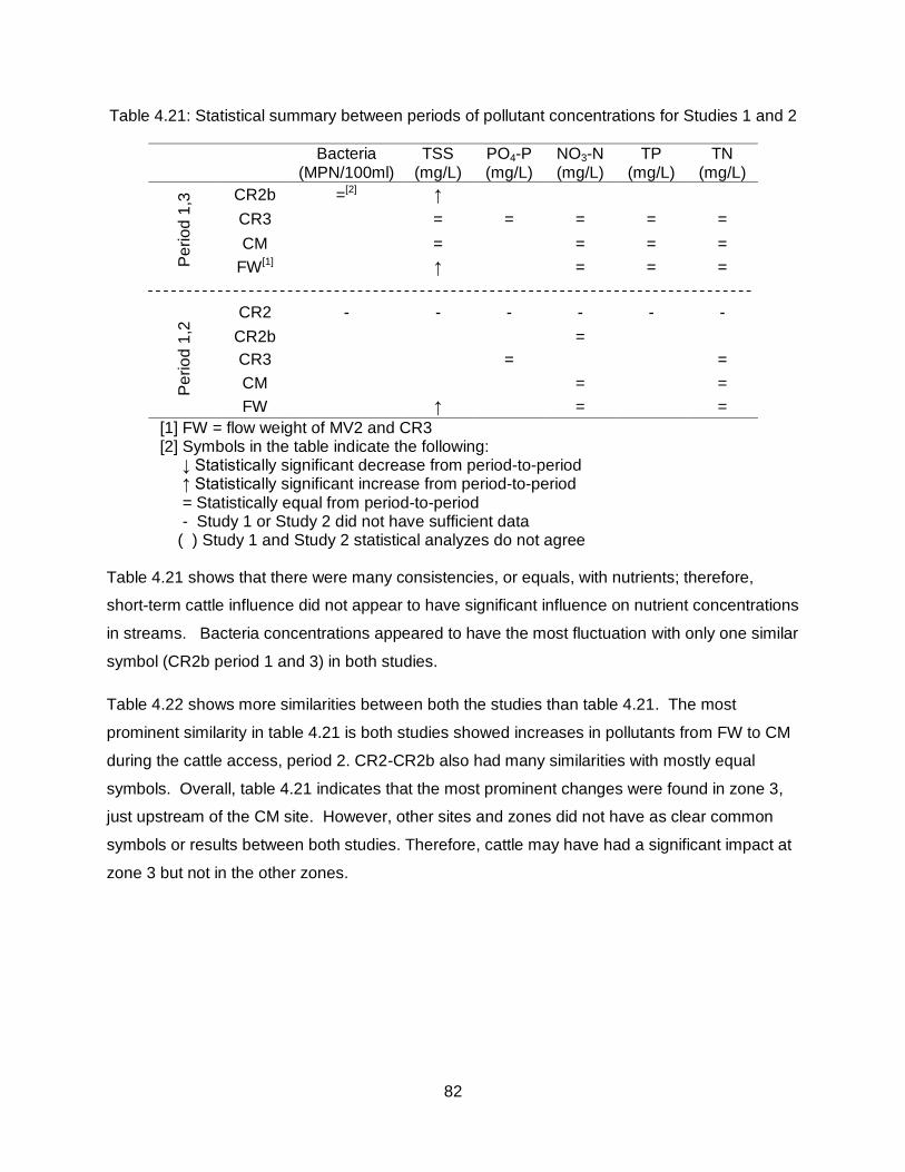
82

Table 4.21: Statistical summary between periods of pollutant concentrations for Studies 1 and 2

Bacteria

(MPN/100ml) TSS

(mg/L) PO4-P (mg/L)

NO3-N (mg/L)

TP (mg/L)

TN (mg/L)

Pe

rio

d 1

,3 CR2b =[2] ↑

CR3

= = = = =

CM

=

= = =

FW[1]

↑

= = =

Pe

rio

d 1

,2 CR2 - - - - - -

CR2b

=

CR3

=

=

CM

=

=

FW

↑

=

=

[1] FW = flow weight of MV2 and CR3 [2] Symbols in the table indicate the following: ↓ Statistically significant decrease from period-to-period ↑ Statistically significant increase from period-to-period = Statistically equal from period-to-period - Study 1 or Study 2 did not have sufficient data ( ) Study 1 and Study 2 statistical analyzes do not agree

Table 4.21 shows that there were many consistencies, or equals, with nutrients; therefore,

short-term cattle influence did not appear to have significant influence on nutrient concentrations

in streams. Bacteria concentrations appeared to have the most fluctuation with only one similar

symbol (CR2b period 1 and 3) in both studies.

Table 4.22 shows more similarities between both the studies than table 4.21. The most

prominent similarity in table 4.21 is both studies showed increases in pollutants from FW to CM

during the cattle access, period 2. CR2-CR2b also had many similarities with mostly equal

symbols. Overall, table 4.21 indicates that the most prominent changes were found in zone 3,

just upstream of the CM site. However, other sites and zones did not have as clear common

symbols or results between both studies. Therefore, cattle may have had a significant impact at

zone 3 but not in the other zones.

83

Table 4.22: Statistical summary of paired sites of pollutant concentrations for Studies 1 and 2

Bacteria

(MPN/100ml) TSS

(mg/L) PO4-P (mg/L)

NO3-N (mg/L)

TP (mg/L)

TN (mg/L)

Pe

rio

d 1

CR2-CR2b -[2] - - - - -

CR2b-CR3 ↓

= =

=

FW[1]-CM ↑ ↑

= =

MV1b-MV2 - - - - - -

Pe

rio

d 2

CR2-CR2b

=

=

CR2b-CR3

= = = = =

FW-CM ↑ ↑ ↑ ↑ ↑ ↑

MV1b-MV2 - - - - - -

[1] FW = flow weight of MV2 and CR3 [2] Symbols in the table indicate the following: ↓ Statistically significant decrease from period-to-period ↑ Statistically significant increase from period-to-period = Statistically equal from period-to-period - Study 1 or Study 2 did not have sufficient data ( ) Study 1 and Study 2 statistical analyzes do not agree

Determining the time it takes for peak concentrations of TSS and E. coli to return to a baseline

condition can help in understanding the differences between unrestricted free cattle access and

flash grazing events. Results show that many of the peak concentrations did not have time to

return to baseline, but the peaks that experienced a 100% recovery, returned to baseline within

one day.

Turbidity was used as an indicator of cattle impact on water quality because it can easily be

seen by the naked eye. Although each zone varied, as a general rule, turbidity increased when

cattle were present in the stream zone. Approximately three or more cows would cause an

increase above baseline.

Storm loads were compared with flash grazing loads to help understand the impact of short-

term cattle access on water quality. Results show that low intensity storms generally had

comparable impact to a flash grazing event at the MV2 site with the exception of Storms III and

V with rainfall intensities of 1.8 in/hr and 2.6 in/hr respectively.

The weekly grab samples were used to assess any pollutant concentration changes in the

system from 2010 to 2011. These samples were statistically analyzed comparing year-to-year

as well as upstream/downstream variation. Results show that there are significant increases in

84

E. coli and significant decreases in EC for the Cub Run sites with a few statistical differences in

TSS and turbidity. The increases in bacteria could be due to the unrestricted cattle access

upstream of CR in the late fall of 2010. There were no significant long-term changes in pollutant

concentrations from the CREP zone to the flash grazing riparian zones. Therefore, flash

grazing may not have a significant impact beyond the initial impact.

In order to understand the impact of cattle on water quality, it is important to understand how the

system would react in a non-cattle impacted setting represented in this project by the CREP

zone. Overall, pollutant concentrations decreased within the CREP zone from CR1-CR2 and

experienced attenuation of bacteria both long-term and short-term impact.

Overall, cattle access to the stream zone caused increases in E.coli and sediment. Zone 1 and

2 results were often inconsistent and did not appear to have any significant changes when cattle

had access to the stream zone. In contrast, zone 3 and 4 showed several instances with

statistically significant increases in all pollutants. The consistency in increases could be due to

the nature of that particular stream section. The stream bed consists of silt particles and fewer

cobbles compared to other parts of Cub Run. Cattle may like to congregate under the riparian

trees because it has a better footing and provides lots of shade.

6 Limitations and Recommendations

There are several limitations associated with this project. For example, the entire stream

riparian zone in this study was not under the camera surveillance. Due to the limited number of

cameras, they were placed in areas that were suspected to have the greatest number of cattle.

However, there may be large influences of cattle in the stream that were not captured and could

help explain discrepancies in the data. Along with having more cameras, it is suggested that all

the cameras be time-lapse. Motion-sensor cameras only take pictures when the sensor is

triggered. However, there may be movement just outside the viewing area that is not recorded.

Having all time-lapse cameras would give a comprehensive view of the entire stream riparian

zone.

Also, in known high priority areas such as zone 3, several cameras were placed pointing in the

same general area so that the entire zone was captured with video. However, this caused

camera viewing areas to overlap. In future studies, it would be beneficial to place flags or other

markers in the riparian zone that would not alter cattle movement but would clearly define which

camera the cow will be counted towards. Similarly, cameras should be positioned in a way that

85

captured two different zones such as in position 7 in this study. Flags or other marking tools

would also be helpful in creating specific boundaries of each zone. It is quite easy to define

zones upstream and downstream of the ISCO, but the riparian bank area is harder to determine.

Counting cattle in the stream was easier for Cub Run since it is a wider stream with manicured

riparian vegetation. In contrast, MV consisted of low flows and banks with very tall, thick

grasses. The tall grasses create a difficulty when trying to define the presence of cattle in the

stream versus just on the riparian area. There is especially an issue when the cow is further

away from the camera and the view gets smaller. Solving this problem might include more

cameras along the reach or again markers in the water that could help identify when a cow is in

the water or not.

The results and conclusions established for this study only represent the characteristics of this

site. Future studies on different cattle exclusion practices would be beneficial to get the overall

effect of short term impact of cattle. In order to establish a comprehensive understanding of

flash grazing, future studies need to establish the effects of cattle beyond the immediate

impacts. For example, the cutting back of banks during flash grazing has the potential to cause

an increase in sediment during times of higher flows. However, once enough evidence is

established, flash grazing may be a beneficial management opportunity for farmers that are

otherwise reluctant to implement cattle exclusion practices.

86

7 References

Agouridis, C. T., D. R. Edwards, S. R. Workman, J. R. Bicudo, B. K. Koostra, J. L. Taraba, and

R. S. Gates. 2004a. Effects of cattle grazing and BMPs on stream water quality. Trans.

ASAE/CSAE.: 042131.

Agouridis, C. T., D. R. Edwards, S. R. Workman, J. R. Bicudo, B. K. Koostra, J. L. Taraba, and

R. S. Gates. 2004b. Influence of BMPs on cattle position preferences. Trans.

ASAE/CSAE: 042182.

Agouridis, C. T., D. R. Edwards, S. R. Workman, J. R. Bicudo, B. K. Koostra, E. S. Vanzant, and

J. L. Taraba. 2005. Streambank erosion associated with grazing practices in the humid

region. Trans. ASAE. 48(1):181-190.

Alison, G. 2007. Australia introduces virtual livestock fencing. Frontiers of Ecology and the

Environ. 5(6):291.

Benham, B. L., Robbins, J.H., Brannan, K.M., Mostaghimi, S., Dillaha, T.A., Pease, J.W., Smith,

E.P. 2005. Development of survey-like assessment tools to assess agricultural best

management practice performance potential. Soil and Water Conserv. 60(5):251-259.

Bewsell, D. R., R. M. Monaghan, and G. Kaine. 2007. Adoption of stream fencing among dairy

farmers in four New Zealand catchments. Environ. Manage. 40(2):201-209.

BLM. 2011. The Taylor Grazing Act. Casper, WY: U.S. Bureau of Land Management.

Department of the Interior. Available at:

http://www.blm.gov/wy/st/en/field_offices/Casper/range/taylor.1.html. Accessed 3

January 2011.

Brannan, K. M., R. M. Mostaghimi, T. A. Dillaha, C. D. Heatwole, M. L. Wolfe, M. Al-Smadi, S.

Shah, and J. Miller. 2001. Big Otter River fecal coliform TMDL: a case study. ASAE

Paper No. 01-2067.

Buckhouse, J. C., and G. F. Gifford. 1976. Water quality implications of cattle grazing on a

semiarid watershed in southeastern Utah. Range Manage. 29(2):109-113.

Elmore, W., and J. B. Kauffman. 1994. Riparian and watershed systems: degradation and

restoration. Soc. for Range Manage.: 212-231.

87

Embry, L. B., M. A. Hoelscher, R. C. Wahlstrom, C. W. Carlson, L. M. Krista, W. R. Brosz, G. F.

Gastler, and O. E. Olson. 1959. Salinity and livestock water quality. South Dakota

Agricultural Experimental Station Bulletin 481.

Follett, R. F. J.L. Hatfield. 2001. Nitrogen in the environment: sources, problems and

management. 2nd ed. San Diego, CA: Elsevier. 17-43.

Franklin, D. H., M. L. Cabrera, Byers H.L., M. M.K., A. J.G., D. E. Radcliffe, M. A. McCann, H. A.

Kuykendall, C. S. Hoveland, and V. H. I. Calvert. 2009. Impact of water troughs on cattle

use of riparian zones in the Georgia Piedmont in the United States. Anim. Sci.(87):2151-

2159.

Frondorf, L. 2001. An investigation of the relationships between stream benthic

macroinvertebrate assemblage conditions and their stressors. MS thesis. Blacksburg,

VA: Virginia Tech, Department of Biological Systems Engineering.

Galeone, D. G., D. J. Low, and R. A. Brightbill. 2006. Effects of streambank fencing of near-

stream pasture land on a small watershed in Lancaster County, Pennsylvania U.S.

Geological Survey Fact Sheet 2006-3112.

Gary, H. L., S. R. Johnson, and S. L. Ponce. 1983. Cattle grazing impact on surface water

quality in a Colorado front range stream. Soil and Water Conserv. 38(2):124-128.

Grandin, T. 2011. Essential topics in animal agriculture: what farmers need to know. Winter

Forage Conference. Virginia Forage and Grassland Council.

Howell, J. M., C. M.S., and C. P.L. 1996. Effect of sediment particle size and temperature on

fecal bacteria mortality rates and the fecal colifrom/fecal streptococci ratio. Environ.

Qual. 25(6):1216-1220.

Hughes, A. H. 2008. The effects of cattle exclusion on stream structure and function. MS thesis.

Blacksburg, VA: Virginia Tech, Department of Biological Sciences.

Hurley, M. A., and M. E. Roscoe. 1983. Automated statistical analysis of microbial enumeration

by dilution series. Appl. Bacteriology. 55:159-164.

James, E., P. Kleinman, T. Veith, R. Stedman, and A. Sharpley. 2007. Phosphorus contributions

from pastured dairy cattle to streams of the Cannonsville Watershed, New York. Soil and

Water Conserv. 62(1):40-47.

88

Jarvie, H. P., P. M. Haygarthb, C. Neala, P. Butlerb, B. Smitha, P. S. Nadena, A. Joynesb, M.

Neala, H. Wickhama, L. Armstronga, S. Harmana, and E. J. Palmer-Felgatea. 2008.

Stream water chemistry and quality along an upland–lowland rural land-use continuum,

southwest England. Hydrol. 350(3-4):215-231.

Johengen, T. H., A. M. Beeton, and D. W. Rice. 1989. Evaluating the effectiveness of best

management practices to reduce agricultural nonpoint source pollution. Lake and

Reserv. Manage. 5(1):63-70.

Larsen, R. E., J. R. Miner, J. C. Buckhouse, and J. A. Moore. 1994. Water-quality benefits of

having cattle manure deposited away from streams. Bioresource Technol. 48(2):113-

118.

Masters, A. L. 2002. Factors influencing the amount of time spend by cattle in

streams:implications for TMDL development. MS thesis. Blacksburg, VA: Virginia Tech,

Department of Biological Systems Engineering.

MDDNR. 2004. Freshwater benthic macroinvertebrates. Annapolis, Maryland.: Maryland

Department of Natural Resources. Available at:

http://www.dnr.state.md.us/streams/pdfs/benthic_macroinvertebrates.pdf. Accessed 3

January 2012.

Miller, J. D., D. Chanasyk, T. Curtis, T. Entz, and W. Willms. 2010. Influence of streambank

fencing with a cattle crossing on riparian health and water quality of the Lower Little Bow

River in Southern Alberta, Canada. Agr. Water Manage. 97(2):247-258.

Miner, J. R., J. C. Buckhouse, and J. A. Moore. 1992. Will a trough reduce the amount of time

hay-fed livestock spend in the stream (and therefore improve water quality)?

Rangelands 14(1):35-38.

Parsons, C. T., P. A. Momont, T. Delcurto, M. McInnis, and M. L. Porath. 2003. Cattle

distribution patterns and vegetation use in mountain riparian areas. Range Manage.

56(4):334-341.

Peppler, M. C., and F. A. Fitzpatrick. 2006. Methods for monitoring the effects of grazing

management on bank erosion and channel morphology, Fever River, Pioneer Farm,

Wisconsin, 2004. Middleton, WA. United States Geological Survey. Available at:

http://pubs.usgs.gov/fs/2005/3134/. Accessed 20 June 2011.

89

Platts, W. S., and R. L. Nelson. 1985. Streamside and upland vegetation use by cattle.

Rangelands 7(1):5-7.

Reynaud, J. Y., B. Tessier, J. P. Auffret, S. Berne, M. De Batist, T. Marsset, and P. Walker.

2003. The offshore quaternary sediment bodies of the English Channel and its Western

Approaches. Quaternary Sci 18(3-4):361-371.

Robillard, P. D., J. C. Clausen, E. G. Flaig, and D. M. Martin. 1992. Research needs and future

vision for nonpoint source projects. Proceedings of the National RCWP Symposium on

10 Years of Controlling Agricultural Nonpoint Source Pollution: The RCWP Experience.

United States Environmental Protection Agency.

Russell, J. 2010. GPS proves useful tool for Leopold Center grazing research. Iowa State

University. Ames, Iowa. Available at http://www.leopold.iastate.edu/news/05-03-

2010/gps-proves-useful-tool-leopold-center-grazing-research. Accessed 20 June 2011.

Scrimgeour, G. J., and S. Kendall. 2002. Consequences of livestock grazing on water quality

and benthic algal biomass in a Canadian natural grassland plateau. Environ. Manage.

29(6):824-844.

Shukla, S. 2000. Impacts of best management practices on nitrogen discharge from a Virginia

coastal plain watershed. PhD diss. Blacksburg, VA: Virginia Tech, Department of

Biological Systems Engineering.

Soupir, M. L. 2003. Release and transport of bacteria and nutrients from livestock manure

applied to pastureland. MS thesis. Blacksburg, VA: Virginia Tech, Department of

Biological Systems Engineering.

Sweeney, B. W., and J. G. Blaine. 2007. Resurrecting the in-stream side of riparian forests.

Journal of Contemporary Water Research & Education 136(1):17-27.

USEPA. 2003. National management measures to control agricultural sources of NPS pollution.

United States Environmental Protection Agency. Washington, D.C. Available at:

http://water.epa.gov/polwaste/nps/agriculture/agmm_index.cfm. Accessed 20 June 2011.

USEPA, 2008. What is a TMDL? Overview of Impaired Waters and Total Maximum Daily Loads

Program. United States Environmental Protection Agency. Washington, D.C. Available

at: http://www.epa.gov/owow/tmdl/overviewoftmdl.html. Accessed 20 January 2011.

90

VADCR. 2011. Virginia's Conservation Reserve Enhancement Program. Virginia Department of

Conservation and Recreation. Richmond, Virginia. Available at:

http://www.dcr.virginia.gov/soil_and_water/crep.shtml. Accessed 29 March 2011.

Vallentine, J. F. 1989. Range developments and improvements. 3rd ed., San Diego, CA.

Brigham Young University Press.

Vesterby, M., and K. S. Krupa. 1997. Major uses of land in the United States. Statistical Bulletin

No. 973. Washington, D.C.

Vidon, P., M. A. Campbell, and M. Gray. 2008. Unrestricted cattle access to streams and water

quality in till landscape of the Midwest. Agr. Water Manage. 95(3):322-330.

Zeckoski, R., B. Benham, and C. Lunsford. 2007. Water quality and economic benefits of

livestock exclusion from streams: experiences from Virginia. In Watershed Management

to Meet Water Quality Standards and TMDLS (Total Maximum Daily Load) Proceedings.

San Antonio, TX. ASABE No. 701P0207.

91

Appendix A. Stage-Discharge Curves

Figure A.1: CR1 2011 stage-discharge curve

Figure A.2: CR3 2011 stage-discharge curve

y = 0.0027e8.518x R² = 0.7609

0

0.1

0.2

0.3

0.4

0.5

0.6

0.7

0.8

0.9

0 0.1 0.2 0.3 0.4 0.5 0.6 0.7

Flo

w (

m3/s

)

Level (m)

y = 0.0009e18.03x R² = 0.567

0

0.05

0.1

0.15

0.2

0.25

0.3

0.35

0.4

0 0.05 0.1 0.15 0.2 0.25 0.3 0.35 0.4

Flo

w (

m3/s

)

Level (m)

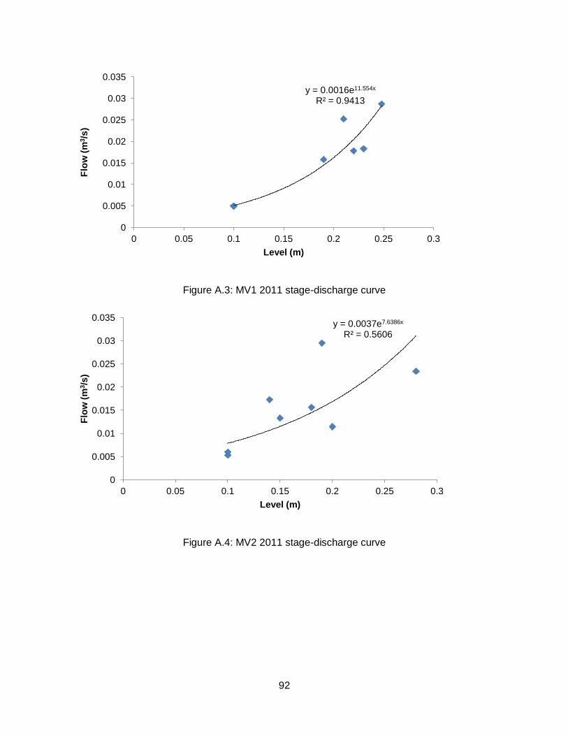
92

Figure A.3: MV1 2011 stage-discharge curve

Figure A.4: MV2 2011 stage-discharge curve

y = 0.0016e11.554x R² = 0.9413

0

0.005

0.01

0.015

0.02

0.025

0.03

0.035

0 0.05 0.1 0.15 0.2 0.25 0.3

Flo

w (

m3/s

)

Level (m)

y = 0.0037e7.6386x R² = 0.5606

0

0.005

0.01

0.015

0.02

0.025

0.03

0.035

0 0.05 0.1 0.15 0.2 0.25 0.3

Flo

w (

m3/s

)

Level (m)

93

Figure A.5: 2010 stage-discharge curves for CR1, CR3, MV1, and MV2

y = 34.919e-29.09x R² = 0.1351

y = 0.0364e-1.102x R² = 0.0011

y = 0.0027e6.2532x R² = 0.6298

y = 0.0007e22.199x R² = 0.8295

0

0.02

0.04

0.06

0.08

0.1

0.12

0.1 0.15 0.2 0.25 0.3 0.35 0.4 0.45

Str

ea

m f

low

(m

3/s

)

Stage (m)

CR1

CR3

MV1

MV2

94

Appendix B. R Statistical Code

This code has been written for the flash grazing study, but only the file and column heading names would be changed to match the years and sites of the weekly grab samples. To test for normality: y<-read.csv("Study1.Bacteria.csv") attach(y) shapiro.test(CR2.1) shapiro.test(CR2b.1) shapiro.test(CR3.1) shapiro.test(CM.1) shapiro.test(FW.1) shapiro.test(MV1b.1) shapiro.test(MV2.1) shapiro.test(CR2.2) shapiro.test(CR2b.2) shapiro.test(CR3.2) shapiro.test(CM.2) shapiro.test(FW.2) shapiro.test(MV1b.2) shapiro.test(MV2.2) shapiro.test(CR2.3) shapiro.test(CR2b.3) shapiro.test(CR3.3) shapiro.test(CM.3) shapiro.test(FW.3) shapiro.test(MV1b.3) shapiro.test(MV2.3) To test for equal variance: bartlett.test(CR2.1) bartlett.test(CR2b.1) bartlett.test(CR3.1) bartlett.test(CM.1) bartlett.test(FW.1) bartlett.test(MV1b.1) bartlett.test(MV2.1) bartlett.test(CR2.2) bartlett.test(CR2b.2) bartlett.test(CR3.2) bartlett.test(CM.2) bartlett.test(FW.2) bartlett.test(MV1b.2) bartlett.test(MV2.2)

95

bartlett.test(CR2.3) bartlett.test(CR2b.3) bartlett.test(CR3.3) bartlett.test(CM.3) bartlett.test(FW.3) bartlett.test(MV1b.3) bartlett.test(MV2.3) To compare period-to-period: wilcox.test(CR2.1, CR2.3) wilcox.test(CR2b.1, CR2b.3) wilcox.test(CR3.1, CR3.3) wilcox.test(CM.1, CM.3) wilcox.test(FW.1, FW.3) wilcox.test(MV1b.1, MV2.3) wilcox.test(MV2.1, MV2.3) wilcox.test(CR2.1, CR2.2) wilcox.test(CR2b.1, CR2b.2) wilcox.test(CR3.1, CR3.2) wilcox.test(CM.1, CM.2) wilcox.test(FW.1, FW.2) wilcox.test(MV1b.1, MV1b.2) wilcox.test(MV2.1, MV2.2) To compare site-to-site: friedman.test(Bacteria, Site, Date.time) pairwise.wilcox.test(Bacteria, Site, p.adj=’bonferroni’, paired=T) In Study 2 where groups had different lengths and could not be compared as a whole: wilcox.test(CR2.1, CR2b.1, p.adj=’bonferroni’, paired=T) wilcox.test(CR2b.1, CR3.1, p.adj=’bonferroni’, paired=T) wilcox.test(FW.1, CM.1, p.adj=’bonferroni’, paired=T) wilcox.test(MV1b.1, MV2.1, p.adj=’bonferroni’, paired=T) wilcox.test(CR2.2, CR2b.2, p.adj=’bonferroni’, paired=T) wilcox.test(CR2b.2, CR3.2, p.adj=’bonferroni’, paired=T) wilcox.test(FW.2, CM.2, p.adj=’bonferroni’, paired=T) wilcox.test(MV1b.2, MV2.2, p.adj=’bonferroni’, paired=T) To find the mean and confidence intervals of two unpaired data sets: y<-read.csv("Study1.Bacteria.csv") attach(y) M=10000 alpha=0.05 bootmean.two=function(CR2b.ln1,CR2b.ln3,M,alpha){ N1=length(CR2b.ln1)

96

N2=length(CR2b.ln3) Med=rep(NA,M) for(i in 1:M){ RS1=sample(CR2b.ln1,N1,replace=TRUE) RS2=sample(CR2b.ln3,N2,replace=TRUE) mean.RS1<-mean(RS1, na.rm=T) mean.RS2<-mean(RS2, na.rm=T) diffRS1.RS2<-(mean.RS1-mean.RS2) Med[i]=diffRS1.RS2 } Iterations<-sum(!is.na(Med)) Boot.est<-mean(Med, na.rm=T) Lower<-quantile(Med, probs=alpha/2, na.rm=T) Upper<-quantile(Med, probs=(1-alpha/2), na.rm=T) Boot.se<-sd(Med, na.rm=T) return(data.frame(Lower, Boot.est, Upper, Boot.se, Iterations)) } bootmean.two(CR2b.ln1,CR2b.ln3,M=10000, alpha=0.05) bootmean.two=function(CM.ln1,CM.ln3,M,alpha){ N1=length(CM.ln1) N2=length(CM.ln3) Med=rep(NA,M) for(i in 1:M){ RS1=sample(CM.ln1,N1,replace=TRUE) RS2=sample(CM.ln3,N2,replace=TRUE) mean.RS1<-mean(RS1, na.rm=T) mean.RS2<-mean(RS2, na.rm=T) diffRS1.RS2<-(mean.RS1-mean.RS2) Med[i]=diffRS1.RS2 } Iterations<-sum(!is.na(Med)) Boot.est<-mean(Med, na.rm=T) Lower<-quantile(Med, probs=alpha/2, na.rm=T) Upper<-quantile(Med, probs=(1-alpha/2), na.rm=T) Boot.se<-sd(Med, na.rm=T) return(data.frame(Lower, Boot.est, Upper, Boot.se, Iterations)) } bootmean.two(CM.ln1,CM.ln3,M=10000, alpha=0.05) bootmean.two=function(FW.ln1,FW.ln3,M,alpha){ N1=length(FW.ln1) N2=length(FW.ln3) Med=rep(NA,M) for(i in 1:M){ RS1=sample(FW.ln1,N1,replace=TRUE) RS2=sample(FW.ln3,N2,replace=TRUE) mean.RS1<-mean(RS1, na.rm=T) mean.RS2<-mean(RS2, na.rm=T) diffRS1.RS2<-(mean.RS1-mean.RS2)

97

Med[i]=diffRS1.RS2 } Iterations<-sum(!is.na(Med)) Boot.est<-mean(Med, na.rm=T) Lower<-quantile(Med, probs=alpha/2, na.rm=T) Upper<-quantile(Med, probs=(1-alpha/2), na.rm=T) Boot.se<-sd(Med, na.rm=T) return(data.frame(Lower, Boot.est, Upper, Boot.se, Iterations)) } bootmean.two(FW.ln1,FW.ln3,M=10000, alpha=0.05) bootmean.two=function(CR2b.ln1,CR2b.ln2,M,alpha){ N1=length(CR2b.ln1) N2=length(CR2b.ln2) Med=rep(NA,M) for(i in 1:M){ RS1=sample(CR2b.ln1,N1,replace=TRUE) RS2=sample(CR2b.ln2,N2,replace=TRUE) mean.RS1<-mean(RS1, na.rm=T) mean.RS2<-mean(RS2, na.rm=T) diffRS1.RS2<-(mean.RS1-mean.RS2) Med[i]=diffRS1.RS2 } Iterations<-sum(!is.na(Med)) Boot.est<-mean(Med, na.rm=T) Lower<-quantile(Med, probs=alpha/2, na.rm=T) Upper<-quantile(Med, probs=(1-alpha/2), na.rm=T) Boot.se<-sd(Med, na.rm=T) return(data.frame(Lower, Boot.est, Upper, Boot.se, Iterations)) } bootmean.two(CR2b.ln1,CR2b.ln2,M=10000, alpha=0.05) bootmean.two=function(CM.ln1,CM.ln2,M,alpha){ N1=length(CM.ln1) N2=length(CM.ln2) Med=rep(NA,M) for(i in 1:M){ RS1=sample(CM.ln1,N1,replace=TRUE) RS2=sample(CM.ln2,N2,replace=TRUE) mean.RS1<-mean(RS1, na.rm=T) mean.RS2<-mean(RS2, na.rm=T) diffRS1.RS2<-(mean.RS1-mean.RS2) Med[i]=diffRS1.RS2 } Iterations<-sum(!is.na(Med)) Boot.est<-mean(Med, na.rm=T) Lower<-quantile(Med, probs=alpha/2, na.rm=T) Upper<-quantile(Med, probs=(1-alpha/2), na.rm=T) Boot.se<-sd(Med, na.rm=T) return(data.frame(Lower, Boot.est, Upper, Boot.se, Iterations))

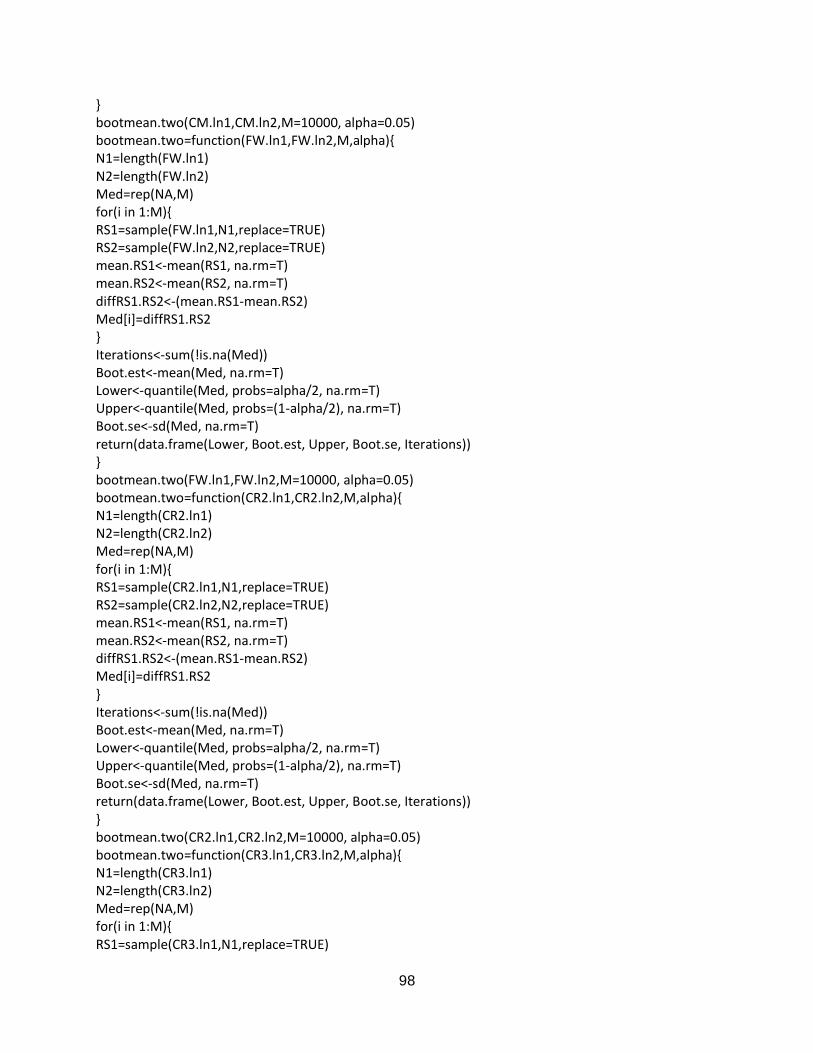
98

} bootmean.two(CM.ln1,CM.ln2,M=10000, alpha=0.05) bootmean.two=function(FW.ln1,FW.ln2,M,alpha){ N1=length(FW.ln1) N2=length(FW.ln2) Med=rep(NA,M) for(i in 1:M){ RS1=sample(FW.ln1,N1,replace=TRUE) RS2=sample(FW.ln2,N2,replace=TRUE) mean.RS1<-mean(RS1, na.rm=T) mean.RS2<-mean(RS2, na.rm=T) diffRS1.RS2<-(mean.RS1-mean.RS2) Med[i]=diffRS1.RS2 } Iterations<-sum(!is.na(Med)) Boot.est<-mean(Med, na.rm=T) Lower<-quantile(Med, probs=alpha/2, na.rm=T) Upper<-quantile(Med, probs=(1-alpha/2), na.rm=T) Boot.se<-sd(Med, na.rm=T) return(data.frame(Lower, Boot.est, Upper, Boot.se, Iterations)) } bootmean.two(FW.ln1,FW.ln2,M=10000, alpha=0.05) bootmean.two=function(CR2.ln1,CR2.ln2,M,alpha){ N1=length(CR2.ln1) N2=length(CR2.ln2) Med=rep(NA,M) for(i in 1:M){ RS1=sample(CR2.ln1,N1,replace=TRUE) RS2=sample(CR2.ln2,N2,replace=TRUE) mean.RS1<-mean(RS1, na.rm=T) mean.RS2<-mean(RS2, na.rm=T) diffRS1.RS2<-(mean.RS1-mean.RS2) Med[i]=diffRS1.RS2 } Iterations<-sum(!is.na(Med)) Boot.est<-mean(Med, na.rm=T) Lower<-quantile(Med, probs=alpha/2, na.rm=T) Upper<-quantile(Med, probs=(1-alpha/2), na.rm=T) Boot.se<-sd(Med, na.rm=T) return(data.frame(Lower, Boot.est, Upper, Boot.se, Iterations)) } bootmean.two(CR2.ln1,CR2.ln2,M=10000, alpha=0.05) bootmean.two=function(CR3.ln1,CR3.ln2,M,alpha){ N1=length(CR3.ln1) N2=length(CR3.ln2) Med=rep(NA,M) for(i in 1:M){ RS1=sample(CR3.ln1,N1,replace=TRUE)

99

RS2=sample(CR3.ln2,N2,replace=TRUE) mean.RS1<-mean(RS1, na.rm=T) mean.RS2<-mean(RS2, na.rm=T) diffRS1.RS2<-(mean.RS1-mean.RS2) Med[i]=diffRS1.RS2 } Iterations<-sum(!is.na(Med)) Boot.est<-mean(Med, na.rm=T) Lower<-quantile(Med, probs=alpha/2, na.rm=T) Upper<-quantile(Med, probs=(1-alpha/2), na.rm=T) Boot.se<-sd(Med, na.rm=T) return(data.frame(Lower, Boot.est, Upper, Boot.se, Iterations)) } bootmean.two(CR3.ln1,CR3.ln2,M=10000, alpha=0.05) bootmean.two=function(CR3.ln1,CR3.ln3,M,alpha){ N1=length(CR3.ln1) N2=length(CR3.ln3) Med=rep(NA,M) for(i in 1:M){ RS1=sample(CR3.ln1,N1,replace=TRUE) RS2=sample(CR3.ln3,N2,replace=TRUE) mean.RS1<-mean(RS1, na.rm=T) mean.RS2<-mean(RS2, na.rm=T) diffRS1.RS2<-(mean.RS1-mean.RS2) Med[i]=diffRS1.RS2 } Iterations<-sum(!is.na(Med)) Boot.est<-mean(Med, na.rm=T) Lower<-quantile(Med, probs=alpha/2, na.rm=T) Upper<-quantile(Med, probs=(1-alpha/2), na.rm=T) Boot.se<-sd(Med, na.rm=T) return(data.frame(Lower, Boot.est, Upper, Boot.se, Iterations)) } bootmean.two(CR3.ln1,CR3.ln3,M=10000, alpha=0.05) To find the mean and confidence intervals of a paired data set: Zone2.ln1<-CR3.ln1-CR2b.ln1 Zone3.ln1<-CM.ln1-FW.ln1 Zone4.ln1<-MV2.ln1-MV1b.ln1 Zone2.ln2<-CR3.ln2-CR2b.ln2 Zone3.ln2<-CM.ln1-FW.ln1 Zone4.ln2<-MV2.ln2-MV1b.ln2 b<-Zone2.ln1[!is.na(Zone2.ln1)] c<-Zone3.ln1[!is.na(Zone3.ln1)] e<-Zone4.ln1[!is.na(Zone4.ln1)] f<-Zone2.ln2[!is.na(Zone2.ln2)] g<-Zone3.ln2[!is.na(Zone3.ln2)]

100

z<-Zone4.ln2[!is.na(Zone4.ln2)] n<-10000 alpha<-0.05 ymean<-numeric(n) for (i in 1:n) { ymean[i]<-mean(sample(b, replace=T)) } quantile(ymean, probs=c(0.025, 0.975), na.rm=T) mean(b) ymean<-numeric(n) for (i in 1:n) { ymean[i]<-mean(sample(c, replace=T)) } quantile(ymean, probs=c(0.025, 0.975), na.rm=T) mean(c) ymean<-numeric(n) for (i in 1:n) { ymean[i]<-mean(sample(e, replace=T)) } quantile(ymean, probs=c(0.025, 0.975), na.rm=T) mean(e) ymean<-numeric(n) for (i in 1:n) { ymean[i]<-mean(sample(f, replace=T)) } quantile(ymean, probs=c(0.025, 0.975), na.rm=T) mean(f) ymean<-numeric(n) for (i in 1:n) { ymean[i]<-mean(sample(g, replace=T)) } quantile(ymean, probs=c(0.025, 0.975), na.rm=T) mean(g) ymean<-numeric(n) for (i in 1:n) { ymean[i]<-mean(sample(z, replace=T)) } quantile(ymean, probs=c(0.025, 0.975), na.rm=T) mean(z)

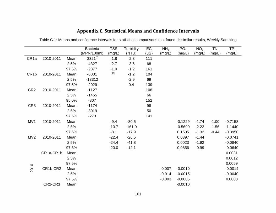
101

Appendix C. Statistical Means and Confidence Intervals

Table C.1: Means and confidence intervals for statistical comparisons that found dissimilar results, Weekly Sampling

Bacteria

(MPN/100ml) TSS

(mg/L) Turbidity (NTU)

EC (μS)

NH3

(mg/L) PO4

(mg/L) NO3

(mg/L) TN

(mg/L) TP

(mg/L)

CR1a 2010-2011 Mean -3321[2] -1.8 -2.3 111

2.5% -4327 -2.7 -3.6 68

97.5% -2377 -1.0 -1.2 161

CR1b 2010-2011 Mean -6001 [1] -1.2 104

2.5% -13312 -2.9 69

97.5% -2029 0.4 139

CR2 2010-2011 Mean -1127 108

2.5% -1465 66

95.0% -807 152

CR3 2010-2011 Mean -1174 98

2.5% -3019

50

97.5% -273

141

MV1 2010-2011 Mean -9.4 -80.5

-0.1229 -1.74 -1.00 -0.7158

2.5% -10.7 -161.9

-0.5690 -2.22 -1.56 -1.1440

97.5% -8.1 -17.9

0.1505 -1.32 -0.44 -0.3950

MV2 2010-2011 Mean -22.4 -26.5

0.0397 -1.44

-0.0741

2.5% -24.4 -41.8

0.0023 -1.92

-0.0840

97.5% -20.0 -12.1

0.0856 -0.99

-0.0640

20

10

CR1a-CR1b Mean

0.0031

2.5%

0.0012

97.5%

0.0059

CR1b-CR2 Mean

-0.007 -0.0010

-0.0014

2.5%

-0.014 -0.0015

-0.0040

97.5%

-0.003 -0.0005

0.0008

CR2-CR3 Mean

-0.0010

102

2.5%

-0.0015

97.5%

-0.0005

MV1-MV2 Mean -21.4

-0.182

-0.0240

2.5% -41.8

-0.325

-0.0447

97.5% -7.6

-0.080

-0.0060

20

11

CR1a-CR1b Mean

2.5%

97.5%

CR1b-CR2 Mean -4540

2.5% -11001

97.5% -974

CR2-CR3 Mean

2.5%

97.5%

MV1-MV2 Mean -17195 -74.5

2.5% -30050 -142.2

97.5% -8633 -18.2

[1] ( ) Non-parametric tests found a similar (p > 0.05) comparison with no need to calculate means and confidence intervals [2] Values were calculated by subtracting upstream from downstream. Thus a negative number indicates a decrease in concentration from upstream to downstream

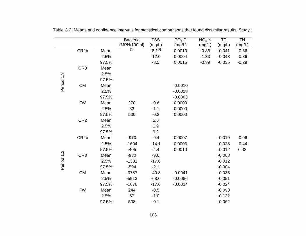
103

Table C.2: Means and confidence intervals for statistical comparisons that found dissimilar results, Study 1

Bacteria

(MPN/100ml) TSS

(mg/L) PO4-P (mg/L)

NO3-N (mg/L)

TP (mg/L)

TN (mg/L)

Pe

rio

d 1

,3

CR2b Mean [1] -8.1[2] 0.0010 -0.86 -0.041 -0.56

2.5% -12.0 0.0004 -1.33 -0.048 -0.86

97.5% -3.5 0.0015 -0.39 -0.035 -0.29

CR3 Mean

2.5%

97.5%

CM Mean -0.0010

2.5% -0.0018

97.5% -0.0003

FW Mean 270 -0.6 0.0000

2.5% 83 -1.1 0.0000

97.5% 530 -0.2 0.0000

Pe

rio

d 1

,2

CR2 Mean 5.5

2.5% 1.9

97.5% 9.2

CR2b Mean -970 -9.4 0.0007 -0.019 -0.06

2.5% -1604 -14.1 0.0003 -0.028 -0.44

97.5% -405 -4.4 0.0010 -0.012 0.33

CR3 Mean -980 -9.6 -0.008

2.5% -1381 -17.6 -0.012

97.5% -594 -2.1 -0.004

CM Mean -3787 -40.8 -0.0041 -0.035

2.5% -5913 -68.0 -0.0086 -0.051

97.5% -1676 -17.6 -0.0014 -0.024

FW Mean 244 -0.5 -0.093

2.5% 57 -1.0 -0.132

97.5% 508 -0.1 -0.062

104

Pe

rio

d 1

CR2-CR2b Mean -1181

2.5% -1794

97.5% -611

CR2b-CR3 Mean -630 0.007

2.5% -885 0.004

97.5% -414 0.010

FW-CM Mean 2903 6.6 0.0032 2.69

2.5% 1687 5.6 0.0028 2.18

97.5% 4247 7.6 0.0036 3.10

Pe

rio

d 2

CR2-CR2b Mean 12.0 -0.0009 0.009

2.5% 8.3 -0.0013 0.004

97.5% 16.2 -0.0006 0.014

CR2b-CR3 Mean

2.5%

97.5%

FW-CM Mean 6945 46.5 0.0073 2.69 0.019 4.03

2.5% 5256 23.8 0.0046 2.22 -0.013 3.52

97.5% 8663 74.4 0.0116 3.09 0.058 4.60

[1] ( ) Non-parametric tests found a similar (p > 0.05) comparison with no need to calculate means and confidence intervals [2] Values were calculated by subtracting upstream from downstream. Thus a negative number indicates a decrease in concentration.

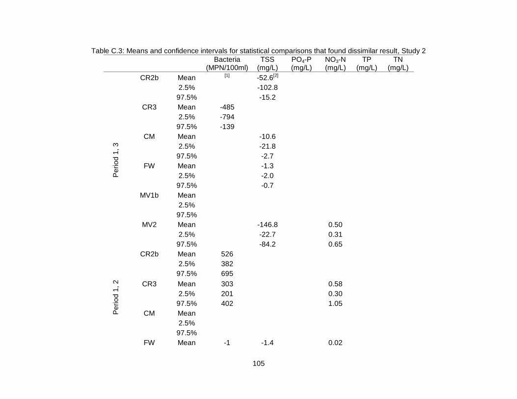
105

Table C.3: Means and confidence intervals for statistical comparisons that found dissimilar result, Study 2

Bacteria (MPN/100ml)

TSS (mg/L)

PO4-P (mg/L)

NO3-N (mg/L)

TP (mg/L)

TN (mg/L)

Pe

rio

d 1

, 3

CR2b Mean [1] -52.6[2]

2.5% -102.8

97.5% -15.2

CR3 Mean -485

2.5% -794

97.5% -139

CM Mean -10.6

2.5% -21.8

97.5% -2.7

FW Mean -1.3

2.5% -2.0

97.5% -0.7

MV1b Mean

2.5%

97.5%

MV2 Mean -146.8 0.50

2.5% -22.7 0.31

97.5% -84.2 0.65

Pe

rio

d 1

, 2

CR2b Mean 526

2.5% 382

97.5% 695

CR3 Mean 303 0.58

2.5% 201 0.30

97.5% 402 1.05

CM Mean

2.5%

97.5%

FW Mean -1 -1.4 0.02

106

2.5% -33 -3.5 0.01

97.5% 21 -0.2 0.03

MV1b Mean -36.6

2.5% -66.1

97.5% -11.8

MV2 Mean -330.4

2.5% -863.9 0.0018

97.5% -27.1 0.0081

Pe

rio

d 1

CR2b-CR3 Mean

2.5%

97.5%

FW-CM Mean 1250 7.3

2.5% 984 6.6

97.5% 1531 7.9

MV1b-MV2 Mean 20.4

2.5% 8.6

97.5% 30.2

Pe

rio

d 2

CR2-CR2b Mean -332

2.5% -524

97.5% -150

CR2b-CR3 Mean -128

2.5% -199

97.5% -45

FW-CM Mean 1695 18.4 0.0066 2.39 0.051 1.29

2.5% 1066 8.1 0.0050 1.93 0.043 1.00

97.5% 2589 35.8 0.0088 2.73 0.061 1.00

MV1b-MV2 Mean 316.3

2.5% 29.4

97.5% 795.9

[1] ( ) Non-parametric tests found a similar (p > 0.05) comparison with no need to calculate means and confidence intervals [2] Values were calculated by subtracting upstream from downstream. Thus a negative number indicates a decrease in concentration

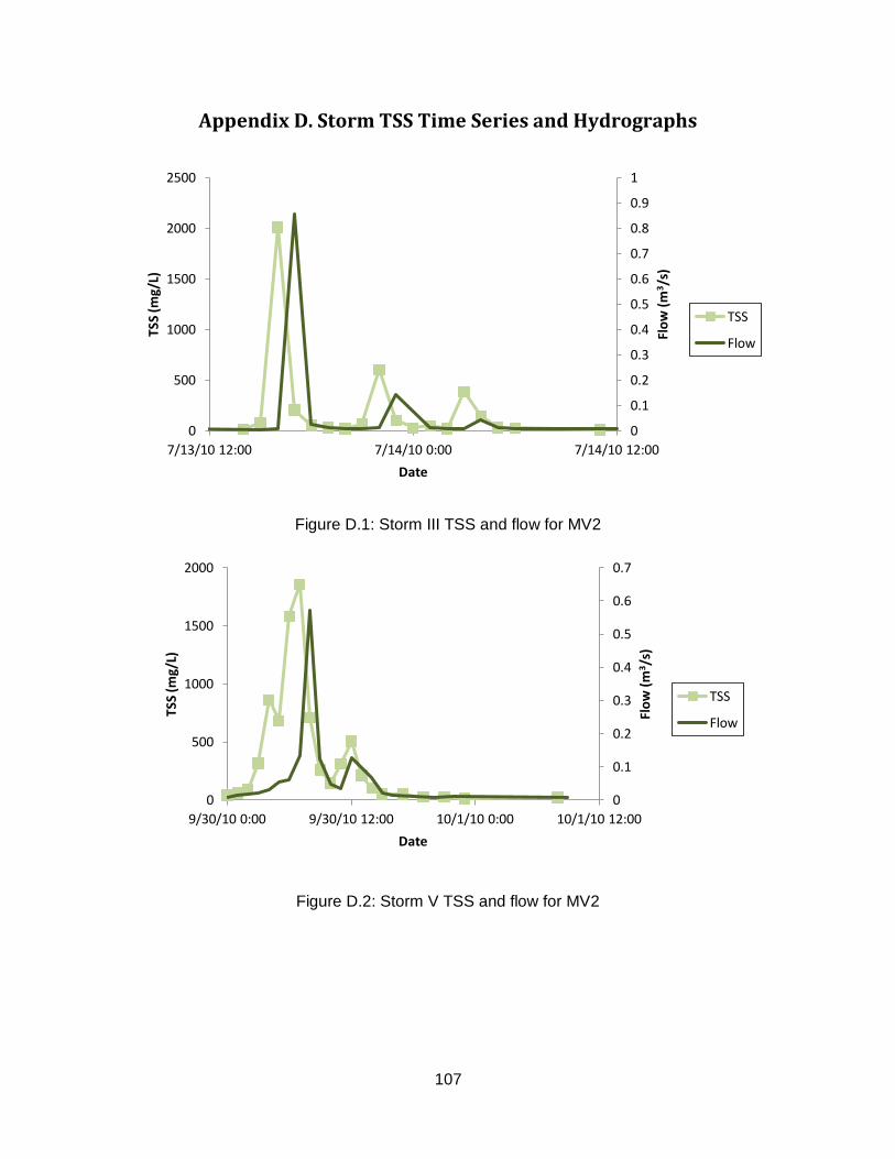
107

Appendix D. Storm TSS Time Series and Hydrographs

Figure D.1: Storm III TSS and flow for MV2

Figure D.2: Storm V TSS and flow for MV2

0

0.1

0.2

0.3

0.4

0.5

0.6

0.7

0.8

0.9

1

0

500

1000

1500

2000

2500

7/13/10 12:00 7/14/10 0:00 7/14/10 12:00

Flo

w (

m3/s

)

TSS

(mg/

L)

Date

TSS

Flow

0

0.1

0.2

0.3

0.4

0.5

0.6

0.7

0

500

1000

1500

2000

9/30/10 0:00 9/30/10 12:00 10/1/10 0:00 10/1/10 12:00

Flo

w (

m3/s

)

TSS

(mg/

L)

Date

TSS

Flow

108

Figure D.3: Storm IX TSS and flow for MV2

Figure D.4: Storm X TSS and flow for MV2

0

0.01

0.02

0.03

0.04

0.05

0.06

0

500

1000

1500

2000

9/5/11 12:00 9/6/11 0:00 9/6/11 12:00 9/7/11 0:00 9/7/11 12:00

Flo

w (

m3/s

)

TSS

(mg/

L)

Date

TSS

Flow

0

0.005

0.01

0.015

0.02

0.025

0.03

0.035

0

50

100

150

200

250

300

350

400

450

10/12/11 0:00 10/12/11 12:00 10/13/11 0:00

Flo

w (

m3/s

)

TSS

(mg/

L)

Date

TSS

Flow

109

Appendix E. Comparing Manual and ISCO Samples

To compare any differences between the ISCO and manual grab samples, coincident samples

were collected using both techniques twice during Study 2. Because the ISCO intake was

located on a plate at the bottom of the stream, there was a greater potential for collecting bed

load when compared to the grab samples that were collected mid-stream and mid-depth.

The comparison samples were analyzed for E. coli, TSS, pH, EC, and turbidity are represented

in figures E.1-E.5. Because pH, EC, and turbidity appeared to be consistent across techniques,

these constituents were not analyzed as rigorously as bacteria and TSS.

Figure E.1: Total suspended solids (TSS) for manual and ISCO grab samples by site

Figure E.2: E. coli bacteria for manual and ISCO grab samples by site

0

10

20

30

40

50

60

70

80

TS

S (

mg

/L)

Site

ISCO

Manual

0

10000

20000

30000

40000

50000

60000

CR

1

CR

1

CR

2

CR

2

CR

2b

CR

2b

CR

3

CR

3

CR

3

CM

CM

CM

MV

1

MV

1

MV

1b

MV

1b

MV

2

MV

2

Ave

rag

e M

PN

/10

0m

l

Site

ISCO

Manual

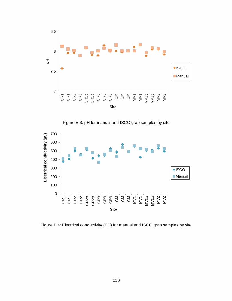
110

Figure E.3: pH for manual and ISCO grab samples by site

Figure E.4: Electrical conductivity (EC) for manual and ISCO grab samples by site

7

7.5

8

8.5

CR

1

CR

1

CR

2

CR

2

CR

2b

CR

2b

CR

3

CR

3

CR

3

CM

CM

CM

MV

1

MV

1

MV

1b

MV

1b

MV

2

MV

2

pH

Site

ISCO

Manual

0

100

200

300

400

500

600

700

CR

1

CR

1

CR

2

CR

2

CR

2b

CR

2b

CR

3

CR

3

CR

3

CM

CM

CM

MV

1

MV

1

MV

1b

MV

1b

MV

2

MV

2

Ele

ctr

ica

l c

on

du

cti

vit

y (

µS

)

Site

ISCO

Manual

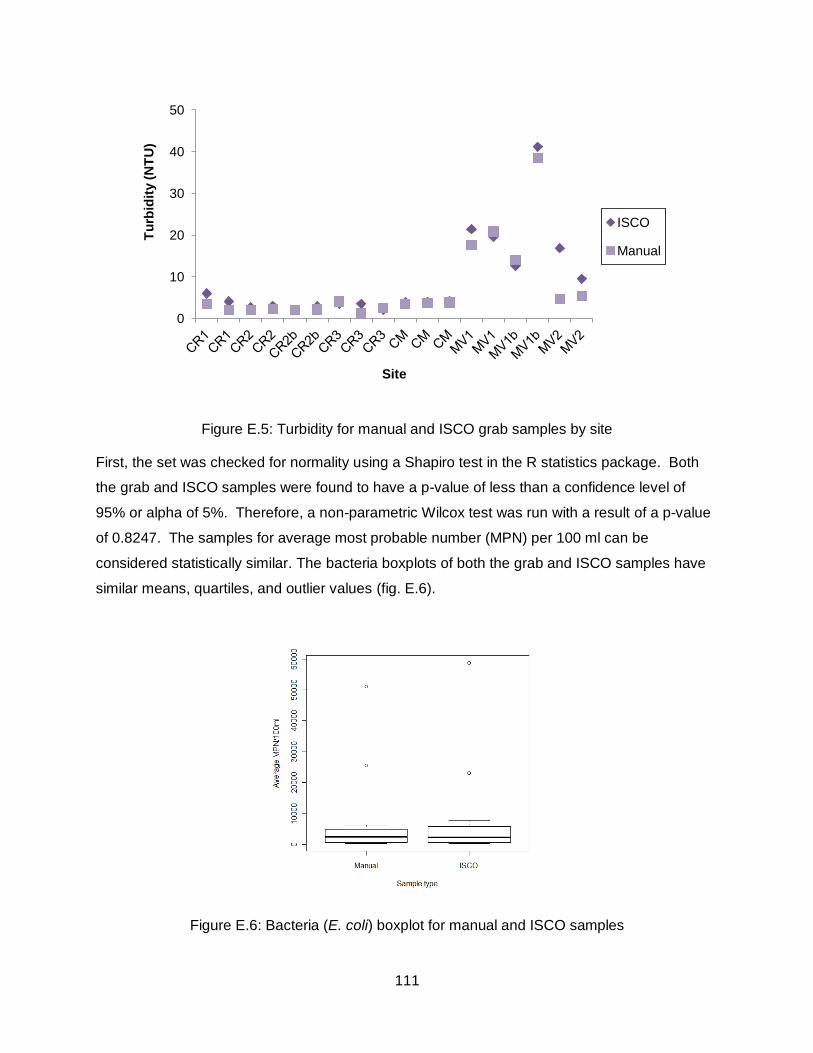
111

Figure E.5: Turbidity for manual and ISCO grab samples by site

First, the set was checked for normality using a Shapiro test in the R statistics package. Both

the grab and ISCO samples were found to have a p-value of less than a confidence level of

95% or alpha of 5%. Therefore, a non-parametric Wilcox test was run with a result of a p-value

of 0.8247. The samples for average most probable number (MPN) per 100 ml can be

considered statistically similar. The bacteria boxplots of both the grab and ISCO samples have

similar means, quartiles, and outlier values (fig. E.6).

Figure E.6: Bacteria (E. coli) boxplot for manual and ISCO samples

0

10

20

30

40

50

Tu

rbid

ity (

NT

U)

Site

ISCO

Manual

112

When graphing bacteria for both sets of the data, the R2 value is 0.989, which means, when

graphed against each other, both have very close correlation and can be considered

comparable (fig. E.7).

Figure E.7: Bacteria (E. coli) plot of manual versus ISCO samples

As in the bacteria, the boxplot of TSS also has similar mean, quartile, and outlier data (fig. E.8).

However, when the grab and ISCO samples are graphed against each other with a one-to-one

line, it can be seen that the ISCO samples over estimate total suspended solids as most of the

points are below the line (fig.E.9). The difference in TSS may mean that there is an influence of

bed load on the ISCO samples causing a higher TSS value than the manual grab samples. The

R2 value of 0.79 is not as significant as the bacteria but can still be considered acceptable.

Therefore, although there are trace differences between the manual and ISCO grab samples,

they can still be considered statistically similar. However, it is important to note that during

times of heavy bed load such as storm events, there may not be as high of a correlation.

R² = 0.989

0

10000

20000

30000

40000

50000

60000

0 10000 20000 30000 40000 50000 60000 70000

Ma

nu

al

Gra

b (

Ave

rag

e M

PN

/10

0m

l)

ISCO Grab (Average MPN/100ml)

113

Figure E.8: TSS boxplot for manual and ISCO samples

Figure E.9: TSS for manual versus ISCO samples and 1:1 line

R² = 0.7929

0

10

20

30

40

50

60

70

80

90

0 20 40 60 80 100

Ma

nu

al

Gra

b T

SS

(m

g/L

)

ISCO Grab TSS (mg/L)

TSS

1:1 line

114

Appendix F. QA/QC

A distilled water grab sample at each of the permanent ISCOs (MV1, MV2, CR1, and CR3) was

taken in order to determine if there were any residual bacteria or sediment in the tubing and

affecting stream water quality results. The data for these samples can be found in figures F.1-

F.4.

Figure F.1: E. coli bacteria for DI blanks by site

Figure F.2: pH for DI banks by site

0

200

400

600

800

1000

1200

1400

1600

CR1 CR3 MV1 MV2

Ave

rag

e M

PN

/10

0m

l

Site

7.0

7.5

8.0

8.5

9.0

CR1 CR3 MV1 MV2

pH

Site

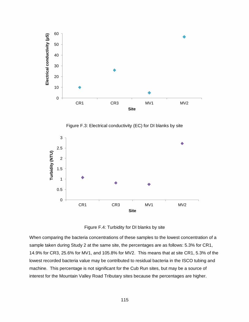
115

Figure F.3: Electrical conductivity (EC) for DI blanks by site

Figure F.4: Turbidity for DI blanks by site

When comparing the bacteria concentrations of these samples to the lowest concentration of a

sample taken during Study 2 at the same site, the percentages are as follows: 5.3% for CR1,

14.9% for CR3, 25.6% for MV1, and 105.8% for MV2. This means that at site CR1, 5.3% of the

lowest recorded bacteria value may be contributed to residual bacteria in the ISCO tubing and

machine. This percentage is not significant for the Cub Run sites, but may be a source of

interest for the Mountain Valley Road Tributary sites because the percentages are higher.

0

10

20

30

40

50

60

CR1 CR3 MV1 MV2

Ele

ctr

ica

l c

on

du

cti

vit

y (

µS

)

Site

0

0.5

1

1.5

2

2.5

3

CR1 CR3 MV1 MV2

Tu

rbid

ity (

NT

U)

Site

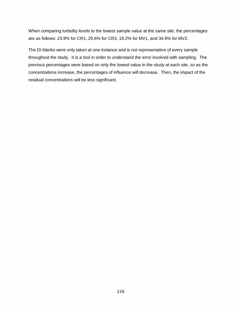
116

When comparing turbidity levels to the lowest sample value at the same site, the percentages

are as follows: 23.9% for CR1, 29.6% for CR3, 19.2% for MV1, and 34.9% for MV2.

The DI blanks were only taken at one instance and is not representative of every sample

throughout the study. It is a tool in order to understand the error involved with sampling. The

previous percentages were based on only the lowest value in the study at each site, so as the

concentrations increase, the percentages of influence will decrease. Then, the impact of the

residual concentrations will be less significant.

117

Appendix G. Salt Tracer Results

The CREP zones and zones 1, 2, and 3 have the approximate travel times: 60 min, 80 min, 50

min, and 50 min, respectively. Mountain Valley Road Tributary has approximately a 45 min

travel time from MV1 to MV2 (unpublished data, 2011. Blacksburg, VA: Virginia Tech,

Department of Biological Systems Engineering). Because samples were a composite of two

hours of stream sample and data were compared within each zone, no lags were applied when

pairing upstream-to-downstream paired data sets. Comparing CR1 to CR2b would have a lag;

however, samples were only tested from the upstream site of each zone to the downstream site.

118

Appendix H. Cattle Densities by Zone

Table H.1: Cattle counts and densities per date and time bottle for zone 1, Study 1

Date/Hr Bottle Max

stream (#)

Ave stream

(#)

Max fencing

(#)

Ave fencing

(#)

Max fencing/area

(#/m2)

Ave fencing/area

(#/m2)

Max stream/length

(#/m)

Ave stream/length

(#/m)

7/21/11 6:00 0 0 1 0.01 0.002 0.000 0 0

7/21/11 18:00 3 0.46 4 1.41 0.002 0.001 0.026 0.004

7/21/11 20:00 0 0 2 0.09 0.005 0.000 0 0

7/22/11 0:00 0 0 1 0.03 0.002 0.000 0 0

7/22/11 8:00 1 0.01 1 0.01 0.000 0.000 0.009 0.000

7/22/11 14:00 5 0.58 10 2 0.004 0.001 0.043 0.005

7/22/11 16:00 2 0.69 7 1.69 0.003 0.001 0.017 0.006

7/22/11 18:00 0 0 4 0.48 0.002 0.000 0 0

7/22/11 20:00 0 0 2 0.05 0.001 0.000 0 0

7/23/11 6:00 4 0.63 13 2.22 0.140 0.010 0.035 0.005

7/23/11 8:00 7 1.07 16 3.23 0.140 0.035 0.061 0.009

7/23/11 14:00 3 0.07 6 0.58 0.003 0.000 0.026 0.001

7/23/11 16:00 3 0.82 6 1.72 0.003 0.001 0.026 0.007

7/23/11 18:00 2 0.08 9 1.03 0.072 0.015 0.017 0.001

7/23/11 20:00 0 0 1 0.02 0.002 0.000 0 0

7/24/11 8:00 9 5.74 14 8.94 0.108 0.056 0.078 0.050

7/24/11 10:00 6 2.12 21 13 0.418 0.210 0.052 0.018

7/24/11 12:00 3 0.26 12 4.71 0.414 0.155 0.026 0.002

7/24/11 14:00 3 1.48 3 1.53 0.001 0.001 0.026 0.013

7/25/11 8:00 0 0 2 0.60 0.005 0.001 0 0

7/25/11 12:00 0 0 4 0.60 0.009 0.001 0 0

7/25/11 16:00 0 0 6 1.45 0.014 0.003 0 0

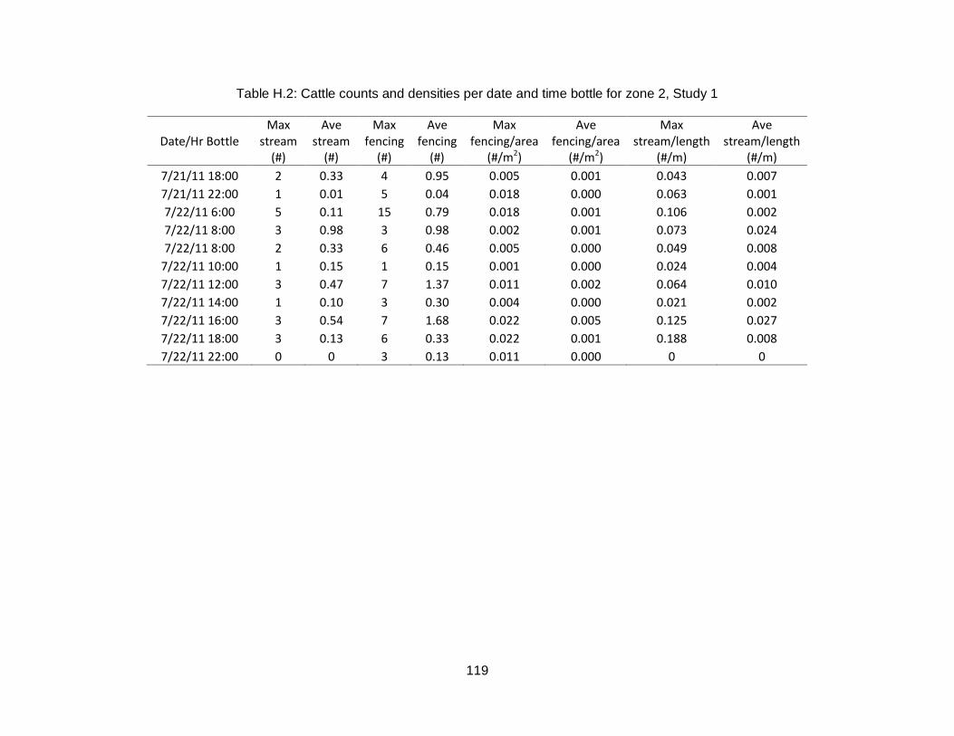
119


Date/Hr Bottle Max

stream (#)

Ave stream

(#)

Max fencing

(#)

Ave fencing

(#)

Max fencing/area

(#/m2)

Ave fencing/area

(#/m2)

Max stream/length

(#/m)

Ave stream/length

(#/m)

7/21/11 18:00 2 0.33 4 0.95 0.005 0.001 0.043 0.007

7/21/11 22:00 1 0.01 5 0.04 0.018 0.000 0.063 0.001

7/22/11 6:00 5 0.11 15 0.79 0.018 0.001 0.106 0.002

7/22/11 8:00 3 0.98 3 0.98 0.002 0.001 0.073 0.024

7/22/11 8:00 2 0.33 6 0.46 0.005 0.000 0.049 0.008

7/22/11 10:00 1 0.15 1 0.15 0.001 0.000 0.024 0.004

7/22/11 12:00 3 0.47 7 1.37 0.011 0.002 0.064 0.010

7/22/11 14:00 1 0.10 3 0.30 0.004 0.000 0.021 0.002

7/22/11 16:00 3 0.54 7 1.68 0.022 0.005 0.125 0.027

7/22/11 18:00 3 0.13 6 0.33 0.022 0.001 0.188 0.008

7/22/11 22:00 0 0 3 0.13 0.011 0.000 0 0

120


Date/Hr Bottle Max

stream (#)

Ave stream

(#)

Max fencing

(#)

Ave fencing

(#)

Max fencing/area

(#/m2)

Ave fencing/area

(#/m2)

Max stream/length

(#/m)

Ave stream/length

(#/m)

7/22/11 4:00 1 0.08 2 0.27 0.002 0.000 0.026 0.002

7/22/11 6:00 12 1.39 24 4.18 0.027 0.004 0.304 0.034

7/22/11 8:00 23 9.70 46 22.62 0.044 0.023 0.582 0.244

7/22/11 10:00 21 15.75 27 20.19 0.032 0.024 0.553 0.414

7/22/11 12:00 15 14.48 25 23.75 0.030 0.029 0.395 0.381

7/22/11 14:00 15 8.34 29 17.03 0.032 0.020 0.395 0.219

7/23/11 6:00 1 0.01 4 0.68 0.003 0.001 0.024 0.000

7/23/11 8:00 20 5.85 24 7.69 0.029 0.009 0.526 0.154

7/23/11 10:00 20 11.61 33 18.21 0.034 0.021 0.526 0.305

7/23/11 12:00 8 2.79 12 6.13 0.014 0.006 0.211 0.069

7/23/11 14:00 0 0 2 0.65 0.002 0.001 0 0

7/23/11 16:00 7 0.32 12 0.48 0.012 0.000 0.180 0.008

7/23/11 18:00 14 5.01 32 12.50 0.029 0.011 0.353 0.121

Table H.4: Cattle counts per date and time bottle for zone 4, Study 1

Date/Hr Bottle Max

stream (#)

Ave stream

(#)

Max fencing

(#)

Ave fencing

(#)

7/22/11 8:00 0 0 1 0.21

7/22/11 14:00 0 0 1 0.30

7/23/11 6:00 0 0 1 0.68

7/23/11 10:00 0 0 1 0.21

7/23/11 12:00 0 0 2 0.21

7/23/11 18:00 1 0.02 4 1.39

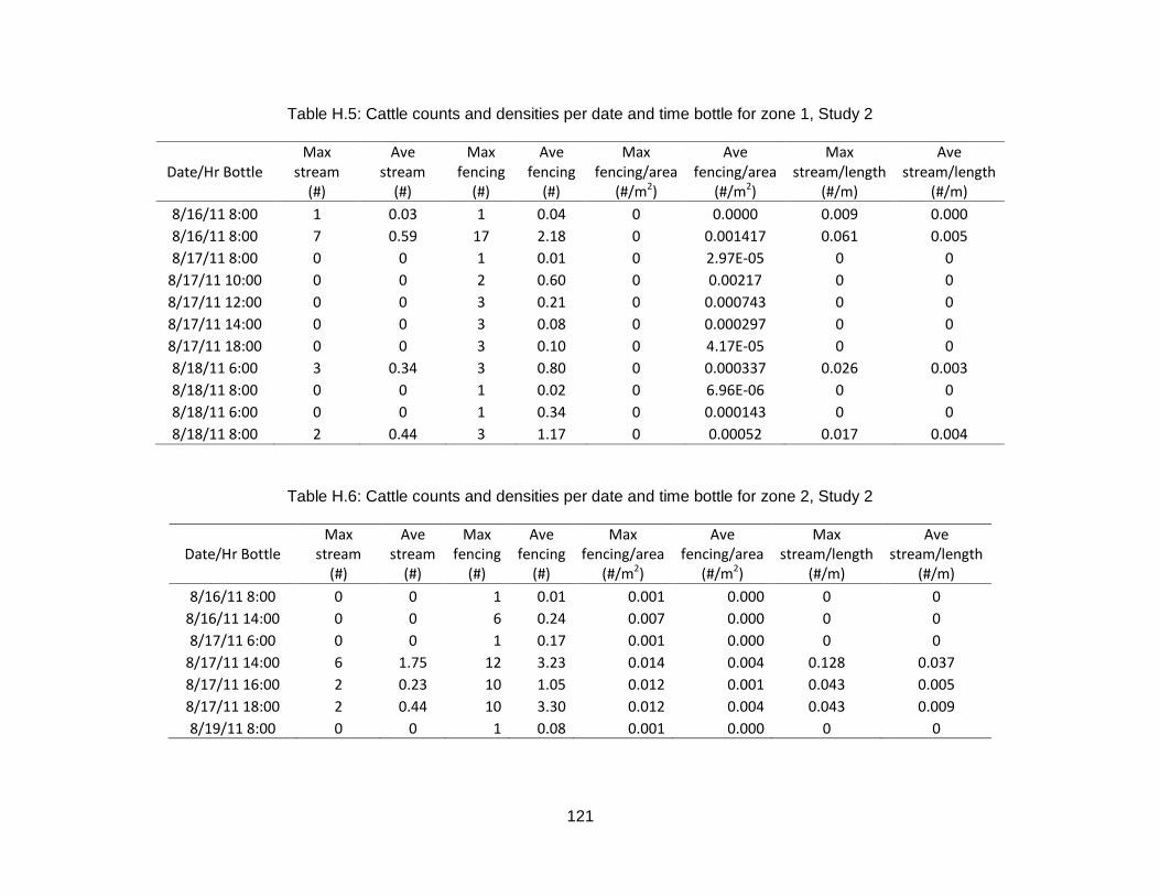
121


Date/Hr Bottle Max

stream (#)

Ave stream

(#)

Max fencing

(#)

Ave fencing

(#)

Max fencing/area

(#/m2)

Ave fencing/area

(#/m2)

Max stream/length

(#/m)

Ave stream/length

(#/m)

8/16/11 8:00 1 0.03 1 0.04 0 0.0000 0.009 0.000

8/16/11 8:00 7 0.59 17 2.18 0 0.001417 0.061 0.005

8/17/11 8:00 0 0 1 0.01 0 2.97E-05 0 0

8/17/11 10:00 0 0 2 0.60 0 0.00217 0 0

8/17/11 12:00 0 0 3 0.21 0 0.000743 0 0

8/17/11 14:00 0 0 3 0.08 0 0.000297 0 0

8/17/11 18:00 0 0 3 0.10 0 4.17E-05 0 0

8/18/11 6:00 3 0.34 3 0.80 0 0.000337 0.026 0.003

8/18/11 8:00 0 0 1 0.02 0 6.96E-06 0 0

8/18/11 6:00 0 0 1 0.34 0 0.000143 0 0

8/18/11 8:00 2 0.44 3 1.17 0 0.00052 0.017 0.004


Date/Hr Bottle Max

stream (#)

Ave stream

(#)

Max fencing

(#)

Ave fencing

(#)

Max fencing/area

(#/m2)

Ave fencing/area

(#/m2)

Max stream/length

(#/m)

Ave stream/length

(#/m)

8/16/11 8:00 0 0 1 0.01 0.001 0.000 0 0

8/16/11 14:00 0 0 6 0.24 0.007 0.000 0 0

8/17/11 6:00 0 0 1 0.17 0.001 0.000 0 0

8/17/11 14:00 6 1.75 12 3.23 0.014 0.004 0.128 0.037

8/17/11 16:00 2 0.23 10 1.05 0.012 0.001 0.043 0.005

8/17/11 18:00 2 0.44 10 3.30 0.012 0.004 0.043 0.009

8/19/11 8:00 0 0 1 0.08 0.001 0.000 0 0

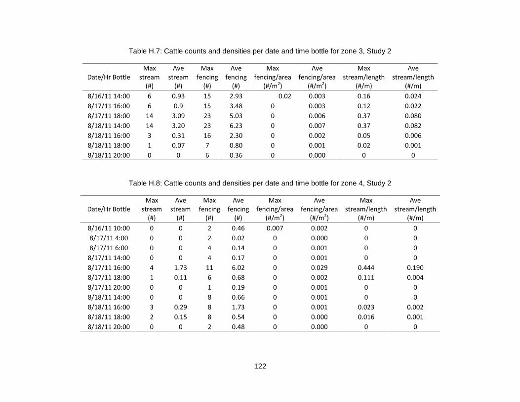
122


Date/Hr Bottle Max

stream (#)

Ave stream

(#)

Max fencing

(#)

Ave fencing

(#)

Max fencing/area

(#/m2)

Ave fencing/area

(#/m2)

Max stream/length

(#/m)

Ave stream/length

(#/m)

8/16/11 14:00 6 0.93 15 2.93 0.02 0.003 0.16 0.024

8/17/11 16:00 6 0.9 15 3.48 0 0.003 0.12 0.022

8/17/11 18:00 14 3.09 23 5.03 0 0.006 0.37 0.080

8/18/11 14:00 14 3.20 23 6.23 0 0.007 0.37 0.082

8/18/11 16:00 3 0.31 16 2.30 0 0.002 0.05 0.006

8/18/11 18:00 1 0.07 7 0.80 0 0.001 0.02 0.001

8/18/11 20:00 0 0 6 0.36 0 0.000 0 0


Date/Hr Bottle Max

stream (#)

Ave stream

(#)

Max fencing

(#)

Ave fencing

(#)

Max fencing/area

(#/m2)

Ave fencing/area

(#/m2)

Max stream/length

(#/m)

Ave stream/length

(#/m)

8/16/11 10:00 0 0 2 0.46 0.007 0.002 0 0

8/17/11 4:00 0 0 2 0.02 0 0.000 0 0

8/17/11 6:00 0 0 4 0.14 0 0.001 0 0

8/17/11 14:00 0 0 4 0.17 0 0.001 0 0

8/17/11 16:00 4 1.73 11 6.02 0 0.029 0.444 0.190

8/17/11 18:00 1 0.11 6 0.68 0 0.002 0.111 0.004

8/17/11 20:00 0 0 1 0.19 0 0.001 0 0

8/18/11 14:00 0 0 8 0.66 0 0.001 0 0

8/18/11 16:00 3 0.29 8 1.73 0 0.001 0.023 0.002

8/18/11 18:00 2 0.15 8 0.54 0 0.000 0.016 0.001

8/18/11 20:00 0 0 2 0.48 0 0.000 0 0

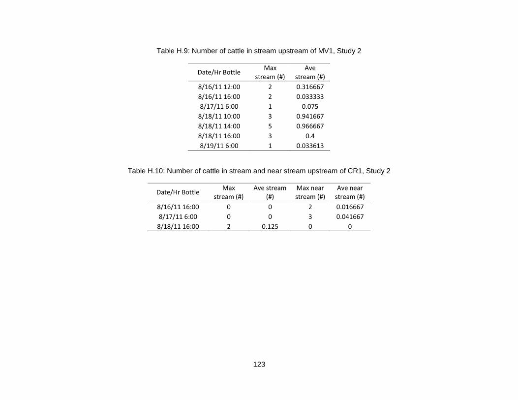
123

Table H.9: Number of cattle in stream upstream of MV1, Study 2

Date/Hr Bottle Max

stream (#) Ave

stream (#)

8/16/11 12:00 2 0.316667

8/16/11 16:00 2 0.033333

8/17/11 6:00 1 0.075

8/18/11 10:00 3 0.941667

8/18/11 14:00 5 0.966667

8/18/11 16:00 3 0.4

8/19/11 6:00 1 0.033613

Table H.10: Number of cattle in stream and near stream upstream of CR1, Study 2

Date/Hr Bottle Max

stream (#) Ave stream

(#) Max near stream (#)

Ave near stream (#)

8/16/11 16:00 0 0 2 0.016667

8/17/11 6:00 0 0 3 0.041667

8/18/11 16:00 2 0.125 0 0

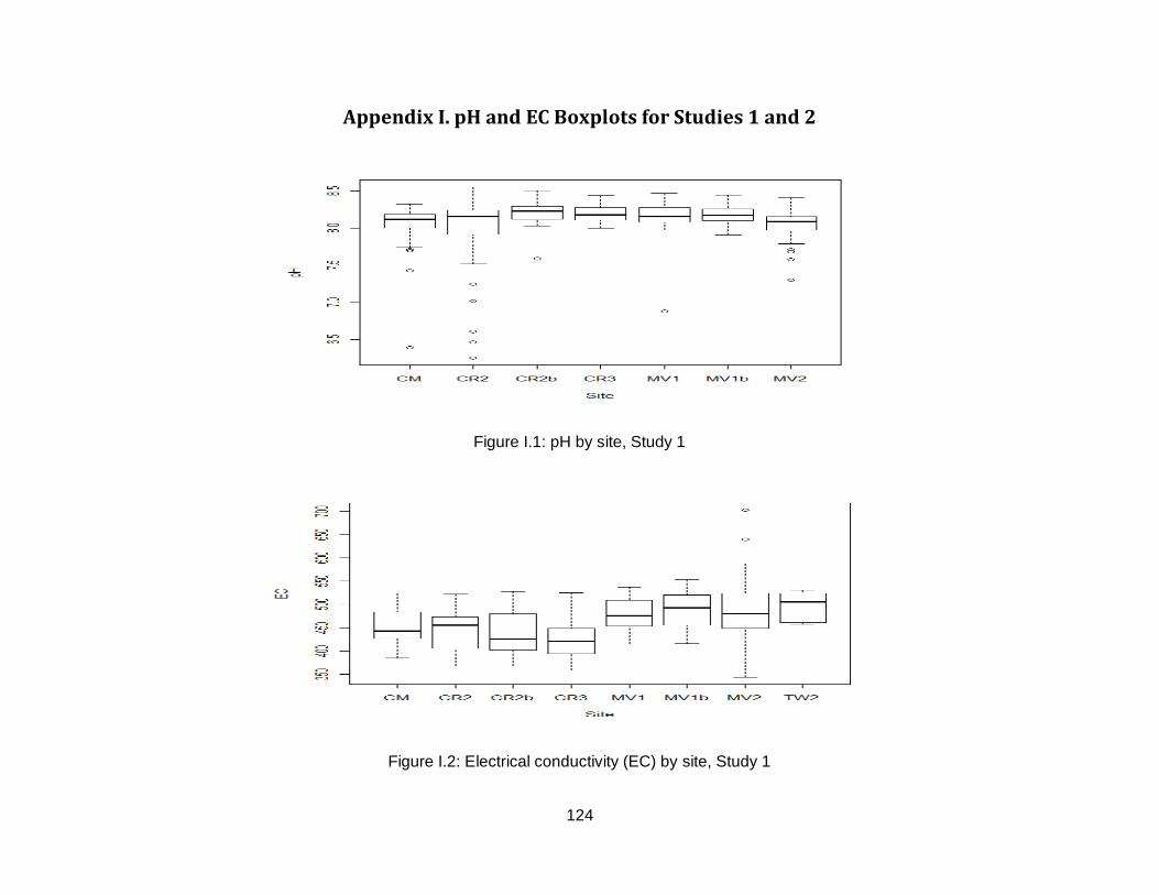
124

Appendix I. pH and EC Boxplots for Studies 1 and 2

Figure I.1: pH by site, Study 1

Figure I.2: Electrical conductivity (EC) by site, Study 1

125

Figure I.3: pH boxplot by site, Study 2

Figure I.4: Electrical conductivity (EC) boxplot by site, Study 2

126

Appendix J. pH, EC, NO3-N, and TN Boxplots for Weekly Grab Samples

Figure I.5: Boxplots of pH for the weekly grab samples by site and year

Figure I.6: Boxplots of electrical conductivity for the weekly grab samples by site and year

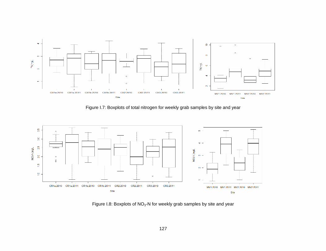
127

Figure I.7: Boxplots of total nitrogen for weekly grab samples by site and year

Figure I.8: Boxplots of NO3-N for weekly grab samples by site and year

Assessing the Effects of Cattle Exclusion Practices on ... · Figure 3.5 Automatic sampler (ISCO...

Documents

Transcript of Assessing the Effects of Cattle Exclusion Practices on ... · Figure 3.5 Automatic sampler (ISCO...