Assessing hybrid monetary function reactions in transition ...

110

El-Hodiri, M., Jawadi, F., & Mukhamediyev, B. (2020). Assessing hybrid monetary function reactions in transition economies. Journal of International Studies, 13(4), 110-127. doi:10.14254/2071-8330.2020/13-4/8

Assessing hybrid monetary function reactions in transition economies

Mohamed El-Hodiri

Department of Economics, Kansas University,

United States of America

[email protected]

Fredj Jawadi

Department of Finance, University of Lille, France [email protected]

Bulat Mukhamediyev

Department of Economics, Al-Farabi Kazakh National University, Kazakhstan [email protected]

Corresponding author

Abstract. This paper specifies and estimates hybrid monetary policy

reaction functions in five countries of the Eastern Europe (Bulgaria,

Czech Republic, Hungary, Poland, and Romania) and four post-

Soviet countries (Belarus, Russia, Kazakhstan, and Ukraine) during

the transition period. The problem of choosing an effective

monetary policy is essential and is of significant interest in

developing economies. The assessed reactions made it possible to

compare monetary policy goals in these countries and their changes

due to the recent global financial and economic crisis. The

calculations carried out by the generalized method of moments

based on the quarterly data for 1998-2018 showed that in all the

countries under consideration, price containment was the primary

goal of monetary policy. Along with it, monetary authorities adhered

to their alternative goals. Moreover, due to the financial and

economic crisis, countries mainly began to less support economic

growth and the accumulation of gold and foreign exchange reserves

while increasing attention to stabilizing the exchange rate and the real

effective exchange rate.

Received: December, 2019

1st Revision: August, 2020

Accepted: December, 2020

DOI: 10.14254/2071-

8330.2020/13-4/8

Journal of International

Studies

Sci

enti

fic

Pa

pers

© Foundation of International

Studies, 2020 © CSR, 2020

mailto:[email protected]

https://mail.google.com/mail/u/0/h/12ep43qol8shj/?&cs=wh&v=b&[email protected]

mailto:[email protected]

Mohamed El-Hodiri, Fredj Jawadi, Bulat Mukhamediyev


111

Keywords: hybrid monetary policy rule, transition countries, global

financial crisis, Eastern Europe, the Commonwealth of Independent

States.

JEL Classification: E52, C54

1. INTRODUCTION

Monetary policy has been an important question in the center of long-lasting economic debates among

many different economists. While John M. Keynes preferred it to improve the global demand and fight the

Great Economic Depression in the 1930s (Keynes, 1936), Milton Friedman has found it effective only in

the short term. See his hypothesis of adaptive expectations (Friedman, 1956). More radically, monetary

policy does not appear to be effective in the short and long terms for Robert Lucas, given his hypothesis of

rational expectations. Monetarist and neoclassical economists stipulate that monetary policy would only

yield inflation tension with no significant effect on the real economy.

Policymakers have always tried to conduct an efficient and rigorous monetary policy to improve central

bank actions' efficiency through effective economic cycle action. At least in the most developed economies,

each central bank has publicly defined the purpose of its action and the conduct of its policy through an

explicit rule. In particular, since Taylor's (1993) eminent paper, a well-known rule – called Taylor Rule has

been developed and adopted by several central banks to conduct their monetary policy. This rule suggests

that the central bank defines the short-term interest rate-setting in relation to the output gap, the inflation

target, and the long-term interest rate. However, some structural breaks in the monetary policy conduct

have taken place, for example, after the UK and New Zealand officially adopted the inflation targeting

policy. Also, given the independent character of central banks, at least till the recent global financial crisis

(2008-2009), central banks in developed countries (i.e., the Fed, the ECB), have tried to stay faithful to their

policies even during the most turbulent times. Since the global financial crisis, several central banks,

including the Fed, the ECB, and the Bank of England, have switched to unconventional monetary policy to

better limit the crisis effect and stimulate their economies. In practice, monetary policy's conduct, at least

until the recent global financial crisis, depended on the central bank and alternating between implicit and

explicit inflation targeting. This was more transparent in developed countries due to the hybrid mandates

of their central banks (Fed, BoE, ECB). In emerging economies, central banks have always conducted

monetary policy to look beyond inflation and the stability of their exchange rates. Many studies have covered

monetary policy conduct by policymakers in these regions (Fiolsa, 2001; Corbo, 2002; Mohanty & Klau,

2005; Jawadi et al., 2014).

In other countries, such as in Eastern Europe (EE) and the Commonwealth of Independent Countries

(CIS), monetary policy has experienced different episodes. These economies have known mutations and

shifts. During their transition process, the EE countries have created their first functioning financial

systems, developed their banking systems, and started to implement a monetary policy process. The latter

has evolved when these economies have switched from fixed to floating exchange rate regimes (Frömmel

& Schobert, 2006). As for the CIS countries, the objective of price stability has always been a challenge.

These economies experienced a hyperinflation episode in the first half of the 1990s because of the ruble

area's dissolution. Straight after that, inflation went up to a two-digit level after introducing new currencies

and adopting a stabilizing program. The monetary policy's conduct has also been affected by the financial

crisis of 1998-1999 and more recently — by the recent global financial crisis (Dabrowski, 2013), pushing

the post-Soviet central banks to follow hybrid monetary policies.

Journal of International Studies

Vol.13, No.4, 2020

112

The following studies considered different issues related to monetary policy. Using correlation analysis

of the Polish economy data, 2005-2017, Redo & Siemiatkowski (2019) showed that the National Bank's

monetary policy affects companies' cost of working capital through changes in interest rates. Shkolnyk et al.

(2019), based on the panel 2007-2017 data for Ukraine, Moldova, and Georgia, assessed the relationship

between growth and employment, exports, the ratio of M1 to GDP, the Gini index, and other indicators.

Using a nonlinear distributed lag autoregressive model for Indonesia data from 1970-2017, Sriana (2019)

found that government spending, money supply, and exchange rate significantly affect inflation. Moreover,

based on the Divisia aggregate for estimating the demand for money in Malaysia, Leong et al. (2019) used a

nonlinear autoregressive method with a distributed lag and data from 1991-2018 to reveal the asymmetric

effects of exchange rate changes.

The rest of the paper consists of four sections. Section 2 provides an overview of the literature on

monetary policy rules in the EE and post-Soviet countries. Section 3 presents the specification monetary

rule for transition economies. Section 4 briefly presents the data and the main empirical results. Section 5

concludes.

2. RELATED LITERATURE

We briefly comment on some of the general papers focusing on monetary policy rules. Papadamou et

al. (2018), using the GMM method, investigated whether the Taylor rule has been applied in all to all

members of the European Union. They concluded that no rule applies to all these countries. Based on the

panel cointegration model and the data from 1999-2012, Arlt & Mandel (2014) showed that the past and

present values of explanatory variables could explain the behavior of interest rates of Poland, Hungary, and

Czech Republic central banks. Owusu (2020), using the GMM method on monthly data from 2003-2018,

found that the European Central Bank's short-term interest rate affects the Swedish Central Bank's

monetary policy.

On the other hand, there are only a few studies of monetary policy rules for post-Soviet countries.

Hybrid policies are rarely studied for these countries. One study is that of Dabrowski (2013), where it is

shown that hybrid policies failed to maintain price stability and provide an effective anti-inflation action.

Furthermore, central banks' independence in these regimes does not seem to be the case. This yields a

fundamental monetary policy challenge in this region.

For example, throughout 1999-2003, Vdovichenko & Voronina (2006) checked Russia's monetary

policy. They showed that the central bank employs a discretionary policy towards the exchange rate rather

than follow a policy of inflation targeting. Esanov et al. (2005) assert that, over the period 1993-2002, a

simple Taylor rule fails to reproduce the Russian monetary policy. They recommend following the

McCallum (1993) rule. According to Ghatak & Moore (2011), the failure of using interest rates in the EE

and post-Soviet economies points to the superiority of the monetary base instrument. However, while the

latter provides positive results during the transition period, the use of interest rates seems to achieve

monetary policy goals over recent years. As far as Kazakhstan is concerned, Mukhamediyev (2007) showed

that while the central bank has employed the monetary base instrument before 2000, its monetary policy

switched to using the short-run interest rate over 2000-2006. Investigating the conduct of monetary policy

in 12 countries in transition over the period 1992-2002, Drobyshevski et al. (2003) showed that central banks

almost always take monetary actions that do not correspond to their declared purposes. El-Hodiri &

Mukhamediyev (2014) also have reached the same conclusion for different economies in transition. In the

same research line, Mohanty & Klau (2005) investigated monetary policy in 13 developing and transition

economies in Asia, Latin America, Africa, and Eastern Europe, including Hungary, Poland, and the Czech

Republic. The authors concluded that although most central banks have focused on fighting inflation, they



113

have changed their interest rates to protect exchange rates' parity. Thus, overall, no unanimous conclusion

does result from these previous studies.

This paper assesses monetary policies in five countries of Eastern Europe (Bulgaria, Czech Republic,

Hungary, Poland, Romania) and four principal post-Soviet countries (Belarus, Russia, Kazakhstan, Ukraine).

Different known mutations and changes over the last decades of those economies have justified selecting

this sample. Further, we develop and estimate different flexible and hybrid monetary rules for these

economies to understand better the reaction in terms of their central banks' monetary functions. In

particular, we check the hypothesis of hybrid monetary policies highlighted by several previous related

studies and test whether monetary policy's conduct varies with the business cycle phase. Finally, we compare

the monetary authorities' different actions and assess each policy rule's advantages and disadvantages.

3. THE MODEL OF MONETARY POLICY RULES FOR TRANSITION ECONOMIES

Each monetary authority always has direct objectives (i.e., inflation control) and indirect objectives (i.e.,

unemployment fighting, exchange rate control, and economic growth stimulation). Accordingly, the central

bank always uses different instruments (i.e., interest rate, open market operation, etc.). To do this, the central

bank often defines well-known monetary policy rules (Taylor Rule, McCullum Rule, etc.). Formally, Clarida

et al. (1998) specified the monetary policy rule as follows:

𝑖𝑡∗ = 𝛼 + 𝛽[𝐸𝑡(𝜋𝑡+𝑛|𝛺𝑡) − 𝜋∗] + 𝛾[𝐸𝑡(𝑦𝑡|𝛺𝑡) − 𝑦𝑡

∗] + 𝛿[𝐸𝑡(𝑧𝑡|𝛺𝑡) − 𝑧𝑡∗], (1)

where: 𝜋𝑡+𝑛 denotes the inflation rate in the period t n . 𝜋∗ denotes the target value of the inflation rate.

𝑦𝑡 is the real output and 𝑦𝑡∗ represents its target value. 𝛺𝑡 refers to the information set available for the

central bank at the time t. 𝐸𝑡 denotes the operator of expectations at the time t based on the information

set 𝛺𝑡. 𝑧𝑡∗ refers to the target value of alternative variable 𝑧𝑡. The term 𝛼 denotes the desired value of the

instrument 𝑖𝑡∗, provided the inflation, output and alternative target variable reached their desired levels. 𝛽, 𝛾,

and 𝛿 are parameters to be estimated.

However, in practice, central banks do not prefer abrupt changes in interest rates, and the following

partial correction mechanism is rather preferred:

𝑖𝑡 = (1 − 𝜌)𝑖𝑡∗ + 𝜌𝑖𝑡−1 + 𝜈𝑡 . (2)

The parameter 𝜌 determines the degree of inertia of the instrument 𝑖𝑡 and thus the degree of

smoothing of interest rate dynamics, while 𝜈𝑡 is a random disturbance. For illustration, the value of 𝜌 for

the developed countries such as the US, Germany, Japan, the UK, France, and Italy, is approximately equal

to 0.95, indicating high inertia of the interest rate dynamics.

Let us substitute 𝑖𝑡∗ from equation (1) into equation (2), we can specify the monetary policy rule as

follows:

𝑖𝑡 = (1 − 𝜌)𝛼 + (1 − 𝜌)𝛽𝜋𝑡+𝑛 + (1 − 𝜌)𝛾𝑦𝑡 + (1 − 𝜌)𝛿𝑧𝑡 + 𝜌𝑖𝑡−1 + 𝜂𝑡 , (3)

where:

𝜂𝑡 = (1 − 𝜌)[𝛽(𝐸𝑡(𝜋𝑡+𝑛|𝛺𝑡) − 𝜋𝑡+𝑛) + 𝛾(𝐸𝑡(𝑦𝑡|𝛺𝑡) − 𝑦𝑡) + 𝛿(𝐸𝑡(𝑧𝑡|𝛺𝑡) − 𝑧𝑡)] + 𝜈𝑡 .


Vol.13, No.4, 2020

114

The model used in the paper is based on the Clarida et al. (1998) model but differs from it, which is

explained by the features of the statistical data of the emerging economies of the post-Soviet countries and

Eastern Europe. In equation (3) 𝑖𝑡 , 𝜋𝑡+𝑛, 𝑦𝑡 , 𝑧𝑡 , and 𝜂𝑡 are random variables. Let 𝑖̌𝑡, �̌�𝑡+𝑛, �̌�𝑡 , �̌�𝑡 , and �̌�𝑡

are means of the corresponding random variables at period 𝑡. Besides, �̌�𝑡 is assumed zero. Then by taking

the mean of both sides of the equation (3), we get the equation:

𝑖�̌� = (1 − 𝜌)𝛼 + (1 − 𝜌)𝛽�̌�𝑡+𝑛 + (1 − 𝜌)𝛾�̌�𝑡 + (1 − 𝜌)𝛿�̌�𝑡 + 𝜌𝑖�̌�−1. (4)

Subtracting (4) from (3), we get the following monetary rule:

𝑖̃𝑡 = (1 − 𝜌)𝛽�̃�𝑡+𝑛 + (1 − 𝜌)𝛾�̃�𝑡 + (1 − 𝜌)𝛿�̃�𝑡 + 𝜌𝑖̃𝑡−1 + 𝜂𝑡 , (5)

where: 𝑖�̃� = 𝑖𝑡 − 𝑖̌𝑡, �̃�𝑡 = 𝜋𝑡 − �̌�𝑡 , �̃�𝑡 = 𝑦𝑡 − �̌�𝑡 , �̃�𝑡 = 𝑧𝑡 − �̌�𝑡. Thus, equation (5) is similar to the

corresponding equation in Clarida et al. (1998). However, its derivation way is different. Specification (5)

has the advantage of providing a flexible monetary rule. The monetary authority can act on the short-term

interest to control inflation and GDP variations, and other macroeconomic variables (exchange rate, etc.)

in reason of other economic drivers in the term z. Model (5), like Clarida et al. (1998), has a simple form. In

contrast, the calculations showed that the t-statistics of the estimated coefficients in the model (5) do not

take enormous values. Also, model (5) does not contain differences between the current and previous values

of variables and random terms.

4. EMPIRICAL RESULTS

4.1 Data Description

We used the data obtained from the International Financial Statistics of the International Monetary

Fund (IMF) and the Central Statistical Authorities of the nine countries included in this study. Inflation is

measured on a CPI basis. The data is quarterly and covers the period: 1998q1 - 2018q4. A limitation of the

study is the use of quarterly data due to the lack of monthly data for some countries' indicators under

consideration.

We applied the Hodrick-Prescott filter to compute trend variables. We noted hereafter irh, inflh, lgdph,

erh, reerh and resh deviations from trend values of the interest rate (lending rate, percent per annum), the

rate of inflation, the logarithm of real GDP, the nominal exchange rate of the national currency versus the

US dollar, the real effective exchange rate, and the gold and foreign reserves, respectively. Further, in the

notation of these variable, we use the symbols be, bu, cz, hu, kz, pl, ro, ru, and ua to refer to the countries

Belarus, Bulgaria, Czech Republic, Hungary, Kazakhstan, Poland, Romania, Russia, and Ukraine,

respectively. For example, variable plerh denotes the deviation from the trend value of Poland's nominal

exchange rate. Table 1 contains the results of the augmented Dickey-Fuller test for all these time series.



115

Table 1

Augmented Dickey-Fuller statistics for time series

Variable Intervals Variable Intervals Variable Intervals

1998q1

–

2008q4

2009q1 –

2018q4

1998q1 –

2008q4

1998q1 –

2008q4

1998q1 –

2008q4

1998q1 –

2008q4

beirh -2.78** -3.67** huirh -2.30** -4.72** roirh -1.98* -3.23**

beinflh -5.67** -2.76** huinflh -1.32 -3.07** roinflh -2.30** -2.15*

belgdph -1.32 -2.22* hulgdph -0.74 -4.99** rolgdph -0.08 -5.79**

beerh -0.57 -4.83** huerh -2.01* -5.27** roerh -2.38* -4.72**

bereerh -2.54* -4.30** hureerh -3.81** -7.20** roreerh -2.07* -3.38**

beresh -5.90** -3.01** huresh -2.54* -1.64† roresh -2.26* -4.13**

buirh -5.32** -2.38* kzirh -3.09** -3.10** ruirh -3.01** -3.18**

buinflh -3.09** -5.04** kzinflh -3.60** -3.56** ruinflh -8.42** -3.48**

bulgdph -0.52 -4.50** kzlgdph -2.22* -2.84* rulgdph -2.49* -2.72**

buerh -1.85† -4.56** kzerh -1.97* -3.62** ruerh -3.87** -2.81**

bureerh -2.94** -2.99** kzreerh -3.06** -5.78** rureerh -6.10** -3.55**

buresh -5.40** -3.21** kzresh -3.75** -2.33* ruresh -2.55* -2.51*

czirh -5.32** -3.08** plirh -4.03** -4.50** uairh -3.62** -3.32**

czinflh -1.99* -5.13** plinflh -2.96** -2.38* uainflh -2.43* -3.78**

czlgdph -2.06* -5.80** pllgdph -2.17* -5.50** ualgdph -2.18* -4.64**

czerh -2.10* -5.11** plerh -2.67** -5.08** uaerh -2.62** -1.80†

czreerh -4.19** -3.80** plreerh -2.19* -6.15** uareerh -3.53** -3.21**

czresh -2.30* -2.97** plresh -6.07** -3.21** uaresh -2.75** -2.43*

Note ** – significance at a 1-percent level, * – significance at a 5-percent level, † - significance at a 10-percent

level.

Source: own calculation

To detect further monetary policy changes over time, we assessed the rules of monetary policy at two

intervals: the first one - from the first quarter of 1998 to the fourth quarter of 2008 and the second interval

– from the first quarter of 2009 to the fourth quarter of 2018. This choice has the advantage of analyzing

the conduct of monetary policy in economies in transition before and after the recent global financial crisis.

In the data series evolution, the main point of interest is their stationarity. For the 108 data series in Table

1, the unit root hypothesis is not rejected at 5% significance level in 9 cases, 7 of them in the first interval,

and 2 in the second interval. All of these cases are taken into account when evaluating the models in Tables

2-19.

4.2. Estimating Hybrid Monetary Rules

We used the generalized method of moments (GMM) to assess the monetary functions of responses

in each country for each interval. Many researchers of monetary policy rules use this method, for example,

Trung & Kiss (2020), Owusu (2020). When using it, GMM does not require information about the

distribution of the error term. It is applicable for correlations between regressors and error terms and

autocorrelation and heteroscedasticity (Greene, 2012). There are two main conditions for the applicability

of GMM. The stationarity of variables and the absence of overidentifying constraints. As shown in Table 1,

the first condition of the variables' stationarity is satisfied, except for several cases when evaluating the

corresponding models. To check the second condition that there are no specification errors, we use J-


Vol.13, No.4, 2020

116

statistics (Hansen, 1982). To perform all calculations, we used the generalized method of moments with

robust Newey-West estimates.

We used lags of dependent and independent variables as instrumental variables. Moreover, we chose

the instrumental variables' composition to satisfy the condition for the absence of specification errors and

to provide the number of instrumental variables used to be as small as possible. Our choice also provides

that the error in equation (5) does not cover the previous period.

We report the main empirical results, including J-statistics in Tables 2-19. In each Table, in the first

column, we specify the list of explanatory variables. The next column (a) shows the estimated coefficients

of the base model without alternative target variables. Column (b) shows the estimated coefficients of the

base model with an additionally included output variable. Finally, the last three columns (c) - (e) show the

base model's estimated coefficients, including exchange rate variables, real effective exchange rate, and gold

and foreign exchange reserves, respectively. Moreover, if in column (b) the output variable's coefficient is

statistically significant and positive, then it is also included in these models.

Regarding the proxy of inflation expectation, we used in all cases ahead of one quarter. According to

the model's specification, the coefficients for output variables and the exchange rate should be positive. The

coefficients for the real effective exchange rate variables and gold and foreign exchange reserves should be

negative. We use bold to show the columns in which all the estimated coefficients are statistically significant,

and their signs correspond to the model's specification.

Next, we briefly analyze the calculation results and compare them with previous studies for all

countries, excluding Belarus and Bulgaria, for which we could not find the relevant data.

Belarus

From Table 2, we note that for equation (a), the coefficient for the inflation variable is significant and

positive. While the output gap's coefficient is statistically not significant when considering the first interval

estimation (equation (b)). This suggests that the central bank policy in Belarus is inflation targeting.

Furthermore, as one can see from equations (c), (d), and (e), the central bank in Belarus can adjust its interest

rate. Therefore, its monetary reaction functions have only changed the real effective exchange rate and the

gold and foreign exchange reserves. The fact that the hypothesis of a unit root (Table 1) is not rejected for

variables belgdph and beerh does not affect these conclusions. This suggests that, before the recent global

financial crisis (2008), the monetary policy in Belarus has aimed at fighting inflation while keeping a close

eye on the variation of the real exchange rate and the foreign exchange reserves.

Table 2

Dependent variable beirh, Interval 1: 1999q1-2008q4

Equation (a) (b) (c) (d) (e)

beirh (-1) 0.972** (.00) 0.984** (.00) 0.722** (.00) 0.825** (.00) 0.998** (.00)

beinflh (+1) 0.082** (.00) 0.085** (.00) 0.023** (.00) 0.115** (.00) 0.073** (.00)

belgdph -0.245 (.79)

beerh -0.000 (.72)

bereerh -0.132** (.00)

beresh -0.006* (.00))

J-statistics 6.26 (.94) 6.25 (.90) 7.08 (.93) 7.51 (.91) 8.00 (0.93)

Note: ** – significance at a 1-percent level, * – significance at a 5-percent level, † - significance at a 10-percent level. The corresponding p-values are shown in parentheses. Source: own calculation

It also appears that in the aftermath of the global financial crisis, the monetary policy remains more

sensitive to changes in inflation than to the output. In column (c) of Table 3, all coefficients are statistically



117

significant, and the coefficient of the exchange rate is negative. Concerning the equation with alternative

targets, the real effective exchange rate variable plays a significant role, suggesting that the monetary

authorities also took into account changes in the real effective exchange rate and reacted in the right

direction.

Table 3

Dependent variable beirh, Interval 2: 2009q1-2018q4


beirh (-1) 0.636** (.00) 0.714**(.00) 0.816** (.00) 0.945** (.00) 0.816** (.00)

beinflh (+1) 0.063** (.00) 0.012 (0.23) 0.086** (.00) 0.037** (.00) 0.097** (.00)

belgdph -22.72**(.00)

beerh -0.0002** (.00)

bereerh -0.192** (.00)

beresh 0.003 (.69)

J-statistics 6.40 (.90) 7.05 (0.90) 7.66 (.91) 5.01 (.93) 7.73 (.90)


Overall, the country's monetary authorities in both intervals sought to stabilize inflation and the real

effective exchange rate, which, according to the data, actually decreased in both intervals. The monetary

policy did not help maintain economic growth and the national currency exchange rate. Although the

interest rate reacted correctly to changes in the gold and foreign exchange reserves in the first interval, the

monetary authorities did not pay much attention to this alternative goal in the second interval. Their decline

replaced the growth of gold and foreign exchange reserves in the second interval.

Bulgaria

From Tables 4 and 5, as in Belarus, the Bulgarian central bank also aims to fight inflation rather pursing

a policy that stimulates economic growth.

Table 4

Dependent variable buirh, Interval 1: 1999q1-2008q4


buirh (-1) 0.803** (.00) 0.788** (.00) 0.363** (.00) -0.066 (.55) 1.802** (.00)

buinflh (+1) 0.026* (.03) 0.019 (.06) 0.001 (.98) 0.011 (.22) -0.083 (.46)

bulgdph -0.849 (.09)

buerh 0.464† (.09)

bureerh 0.097** (.00)

buresh -0.073† (.08))

J-statistics 6.74 (.91) 6.29 (.97) 7.55 (.91) 7.50 (.91) 3.10 (0.96)



Vol.13, No.4, 2020

118

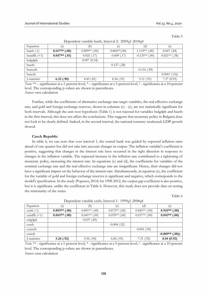
Table 5

Dependent variable buirh, Interval 2: 2009q1-2018q4


buirh (-1) 0.617** (.00) 0.899** (.00) 0.804**(.00) 1.119** (.00) 0.047 (.84)

buinflh (+1) 0.047** (.01) 0.025 (.17) -0.009 (.17) -0.135** (.00) 0.021** (.38)

bulgdph 0.097 (0.34)

buerh 0.127 (.28)

bureerh -0.116 (.50)

buresh 0.006* (.10))

J-statistics 6.32 (.90) 4.45 (.81) 8.36 (.91) 5.11 (.93) 7.57 (0.93)


Further, while the coefficients of alternative exchange rate target variables, the real effective exchange

rate, and gold and foreign exchange reserves, shown in columns (c) - (e), are not statistically significant for

both intervals. Although the unit root hypothesis (Table 1) is not rejected for variables bulgdph and buerh

in the first interval, this does not affect the conclusions. This suggests that monetary policy in Bulgaria does

not look to be clearly defined. Indeed, in the second interval, the national currency weakened; GDP growth

slowed.

Czech Republic

In table 6, we can note that over interval 1, the central bank was guided by expected inflation rates

ahead of one quarter but did not take into account changes in output. The inflation variable's coefficient is

positive, suggesting that changes in the interest rate have occurred in the right direction in response to

changes in the inflation variable. The expected increase in the inflation rate contributed to a tightening of

monetary policy, increasing the interest rate. In equations (c) and (d), the coefficients for variables of the

nominal exchange rate and the real effective exchange rate are insignificant. Hence, their changes did not

have a significant impact on the behavior of the interest rate. Simultaneously, in equation (e), the coefficient

for the variable of gold and foreign exchange reserves is significant and negative, which corresponds to the

model's specification. In the study (Popescu, 2014) for 1998-2012, the output gap coefficient is also positive,

but it is significant, unlike the coefficient in Table 6. However, this study does not provide data on testing

the stationarity of the series.

Table 6

Dependent variable czirh, Interval 1: 1999q1-2008q4


czirh (-1) 0.893** (.00) 0.891** (.00) 0.872** (.00) 0.845** (.00) 0.924** (.00)

czinflh (+1) 0.043** (.00) 0.041** (.00) 0.039** (.00) 0.037** (.00) 0.041** (.00)

czlgdph 0.037 (.83)

czerh -0.004 (.52)

czreerh 0.001 (.95)

czresh -0.009** (.00))

J-statistics 5.26 (.92) 5.56 (.94) 6.06 (.91) 7.31 (.92) 8.04 (0.92)

Note: ** - significance at a 1-percent level, * - significance at a 5-percent level, † - significance at a 10-percent

level. The corresponding p-values are shown in parentheses.




119

Table 7

Dependent variable czirh, Interval 2: 2009q1-2018q4


czirh (-1) 0.901** (.00) 0.759** (.00) 0.886** (.00) 0.914** (.00) 0.791** (.00)

czinflh (+1) 0.010** (.00) 0.011** (.00) 0.004 (.18) -0.006* (.01) 0.011** (.00)

czlgdph -0.021 (.69)

czerh -0.001 (.57)

czreerh -0.0004 (.69)

czresh -8.3E-05 (.50))

J-statistics 4.66 (.95) 7.50 (.91) 7.23 (.95) 4.75 (.96) 8.19 (0.92)




Regarding the second interval, equation (b) with intermediate target inflation and release variables

turned out to be insignificant, and equation (a) only with the inflation target was statistically significant

(Table 7). The country's monetary authorities took into account inflation expectations but did not consider

the changes in output. Equations (c) - (e) with additional alternative target variables are insignificant.

Consequently, in the second interval, the interest rate did not react in the right direction to changes in the

exchange rate, the real effective exchange rate, and the country's gold and currency reserves. Further, for

both intervals, the country's monetary authorities pursued a policy of containing inflation and not aiming to

support economic growth.

Hungary

From Table 8 (equations (a) and (b)), we note that, over the first interval, both inflation and output

gap appear as significant drivers for the monetary policy. However, this conclusion is unreliable since the

unit root hypothesis is not rejected for variables huinflh and hulgdph (Table 1). Further, the central bank

seems not to adjust its interest rate to consider changes in the exchange rate, the real effective exchange

rate, and its gold and currency reserves. Accordingly, in contrast to previous countries, it is unclear whether

the Hungarian Central Bank was able with its mandate to combat price volatility and simultaneously

accelerate economic growth in the first interval. In the results (Popescu, 2014) for 2001-2012, the output

gap's coefficient is negative and significant. However, this may be a consequence of the nonstationarity of

this variable.

Table 8

Dependent variable huirh, Interval 1: 1999q1-2008q4


huirh (-1) 0.389** (.00) 0.885** (.00) 0.992** (.00) 0.815** (.00) 0.773** (.00)

huinflh (+1) 0.165** (.00) 0.115** (.00) 0.169** (.00) 0.109** (.00) -0.008 (.54)

hulgdph 5.767** (.00) 6.313** (.00) 10.53** (.00) -10.58** (.00)

huerh -0.003 (.51)

hureerh 0.037* (.02)

huresh -0.001* (.01)

J-statistics 6.05 (.91) 6.67 (.92) 7.68 (.91) 6.63 (.92) 4.48 (.95)

Note: ** - significance at a 1-percent level, * - significance at a 5-percent level, † - significance at a 10-percent level. The corresponding p-values are shown in parentheses. Source: own calculation


Vol.13, No.4, 2020

120

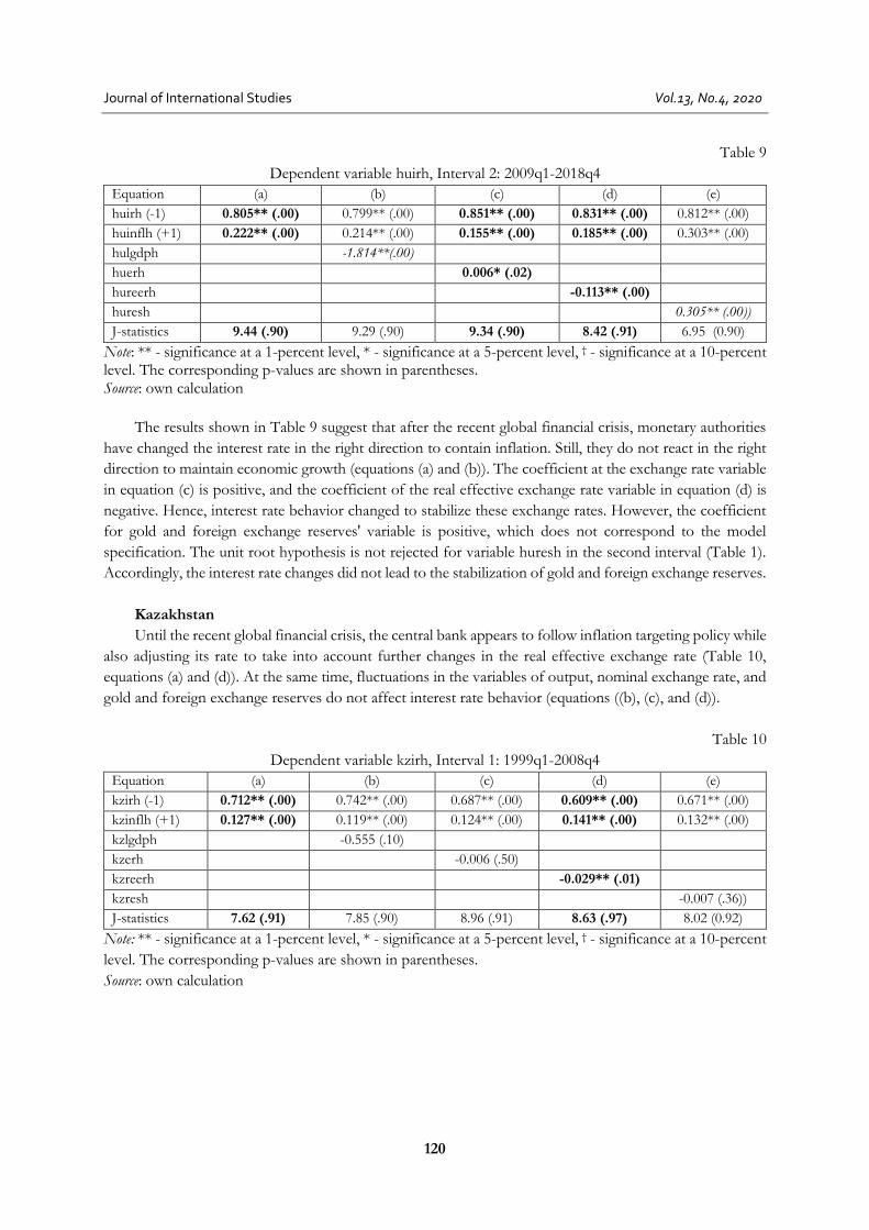
Table 9

Dependent variable huirh, Interval 2: 2009q1-2018q4


huirh (-1) 0.805** (.00) 0.799** (.00) 0.851** (.00) 0.831** (.00) 0.812** (.00)

huinflh (+1) 0.222** (.00) 0.214** (.00) 0.155** (.00) 0.185** (.00) 0.303** (.00)

hulgdph -1.814**(.00)

huerh 0.006* (.02)

hureerh -0.113** (.00)

huresh 0.305** (.00))

J-statistics 9.44 (.90) 9.29 (.90) 9.34 (.90) 8.42 (.91) 6.95 (0.90)


The results shown in Table 9 suggest that after the recent global financial crisis, monetary authorities

have changed the interest rate in the right direction to contain inflation. Still, they do not react in the right

direction to maintain economic growth (equations (a) and (b)). The coefficient at the exchange rate variable

in equation (c) is positive, and the coefficient of the real effective exchange rate variable in equation (d) is

negative. Hence, interest rate behavior changed to stabilize these exchange rates. However, the coefficient

for gold and foreign exchange reserves' variable is positive, which does not correspond to the model

specification. The unit root hypothesis is not rejected for variable huresh in the second interval (Table 1).

Accordingly, the interest rate changes did not lead to the stabilization of gold and foreign exchange reserves.

Kazakhstan

Until the recent global financial crisis, the central bank appears to follow inflation targeting policy while

also adjusting its rate to take into account further changes in the real effective exchange rate (Table 10,

equations (a) and (d)). At the same time, fluctuations in the variables of output, nominal exchange rate, and

gold and foreign exchange reserves do not affect interest rate behavior (equations ((b), (c), and (d)).

Table 10

Dependent variable kzirh, Interval 1: 1999q1-2008q4


kzirh (-1) 0.712** (.00) 0.742** (.00) 0.687** (.00) 0.609** (.00) 0.671** (.00)

kzinflh (+1) 0.127** (.00) 0.119** (.00) 0.124** (.00) 0.141** (.00) 0.132** (.00)

kzlgdph -0.555 (.10)

kzerh -0.006 (.50)

kzreerh -0.029** (.01)

kzresh -0.007 (.36))

J-statistics 7.62 (.91) 7.85 (.90) 8.96 (.91) 8.63 (.97) 8.02 (0.92)






121

Table 11

Dependent variable kzirh, Interval 2: 2009q1-2018q4


kzirh (-1) 0.862** (.00) 0.993** (.00) 0.711** (.00) 0.617** (.00) 0.927** (.00)

kzinflh (+1) 0.217** (.00) 0.248** (.00) 0.110** (.00) 0.099** (.00) -0.039 (.27)

kzlgdph -0.628 (0.61)

kzerh 0.024* (.00)

kzreerh -0.083** (.00)

kzresh -0.026** (.00)

J-statistics 4.84 (.90) 5.94 (0.92) 7.75 (.90) 7.61 (.91) 8.24 (.91)




Interestingly, the monetary authority has followed a similar rule in the aftermath of the recent global

financial crisis. Indeed, the basic equation (a) with a variable of the expectation of inflation and the equation

(d) with real effective exchange rates are statistically significant (Table 11). The interest rate changed in the

right direction in response to fluctuations in the expected inflation rate ahead of one quarter. It did not react

correctly to the current value of the variable of economic growth. In the second interval, the interest rate

responded in the right direction to fluctuations in the nominal exchange rate (equation (c)).

Thus, during both intervals, the monetary authorities attached significant importance to curbing

inflation, stabilizing the real effective exchange rate, and ignored support for economic growth and gold

and foreign exchange reserves. Besides, in the second interval, one of the goals was to stabilize the nominal

exchange rate, as there was a strong tendency to weaken the national currency. Drobyshevsky et al. (2003)

undertook an attempt to assess Kazakhstan's rules based on data from 1993-2002. But it was unsuccessful.

Mukhamediyev (2007) showеd that for the period from 1995-1999, the monetary base, rather than the

interest rate, was a more suitable monetary policy instrument.

Poland

As for Hungary, we found that over the first interval, the monetary policy in Poland fought inflation

and boost economic growth simultaneously (Table 12, equations (a) and (b)). The conduct of monetary

policy following the Taylor rule appears, however, more strict. The coefficients of alternative target variables

of nominal and real effective exchange rates and gold and foreign exchange reserves are insignificant.

Table 12

Dependent variable plirh, Interval 1: 1999q1-2008q4


plirh (-1) 0.837** (.00) 0.831** (.00) 0.789** (.00) 0.781** (.00) 0.833** (.00)

plinflh (+1) 0.405** (.00) 0.383** (.00) 0.233** (.00) 0.456** (.00) 0.354** (.00)

pllgdph 1.139** (.01) 1.320* (.04) -0.330 (.60) 0.112 (.87)

plerh -0.249 (.11)

plreerh 0.015 (.07)

plresh 0.021** (.00)

J-statistics 7.88 (0.90) 7.42 (.92) 7.18 (.93) 7.19 (.93) 7.30 (.0.89)





Vol.13, No.4, 2020

122

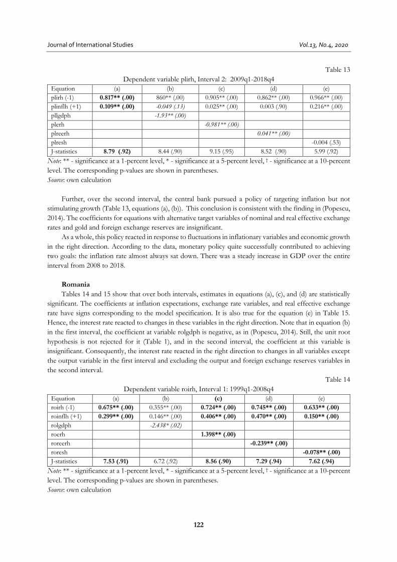
Table 13

Dependent variable plirh, Interval 2: 2009q1-2018q4


plirh (-1) 0.817** (.00) 860** (.00) 0.905** (.00) 0.862** (.00) 0.966** (.00)

plinflh (+1) 0.109** (.00) -0.049 (.13) 0.025** (.00) 0.003 (.90) 0.216** (.00)

pllgdph -1.93** (.00)

plerh -0.981** (.00)

plreerh 0.041** (.00)

plresh -0.004 (.53)

J-statistics 8.79 (.92) 8.44 (.90) 9.15 (.95) 8.52 (.90) 5.99 (.92)




Further, over the second interval, the central bank pursued a policy of targeting inflation but not

stimulating growth (Table 13, equations (a), (b)). This conclusion is consistent with the finding in (Popescu,

2014). The coefficients for equations with alternative target variables of nominal and real effective exchange

rates and gold and foreign exchange reserves are insignificant.

As a whole, this policy reacted in response to fluctuations in inflationary variables and economic growth

in the right direction. According to the data, monetary policy quite successfully contributed to achieving

two goals: the inflation rate almost always sat down. There was a steady increase in GDP over the entire

interval from 2008 to 2018.

Romania

Tables 14 and 15 show that over both intervals, estimates in equations (a), (c), and (d) are statistically

significant. The coefficients at inflation expectations, exchange rate variables, and real effective exchange

rate have signs corresponding to the model specification. It is also true for the equation (e) in Table 15.

Hence, the interest rate reacted to changes in these variables in the right direction. Note that in equation (b)

in the first interval, the coefficient at variable rolgdph is negative, as in (Popescu, 2014). Still, the unit root

hypothesis is not rejected for it (Table 1), and in the second interval, the coefficient at this variable is

insignificant. Consequently, the interest rate reacted in the right direction to changes in all variables except

the output variable in the first interval and excluding the output and foreign exchange reserves variables in

the second interval.

Table 14

Dependent variable roirh, Interval 1: 1999q1-2008q4


roirh (-1) 0.675** (.00) 0.355** (.00) 0.724** (.00) 0.745** (.00) 0.633** (.00)

roinflh (+1) 0.299** (.00) 0.146** (.00) 0.406** (.00) 0.470** (.00) 0.150** (.00)

rolgdph -2.438* (.02)

roerh 1.398** (.00)

roreerh -0.239** (.00)

roresh -0.078** (.00)

J-statistics 7.53 (.91) 6.72 (.92) 8.56 (.90) 7.29 (.94) 7.62 (.94)






123

Table 15

Dependent variable roirh, Interval 2: 2009q1-2018q4


roirh (-1) 0.880** (.00) 0.885** (.00) 0.779** (.00) 0.890** (.00) 0.745** (.00)

roinflh (+1) 0.135** (.00) 0.148** (.00) 0.198** (.00) 0.148** (.00) -0.035 (.16)

rolgdph 0.289 (.19)

roerh 0.447** (.00)

roreerh -0.034* (.03)

roresh -0.046** (.00)

J-statistics 7.01 (.93) 6.20 (.94) 7.45 (.94) 7.61 (.94) 7.94 (.93)


Accordingly, it looks like in Romania, the monetary authorities took into account all the considered

alternative goals and reacted in the right direction, especially in the second interval. The monetary policy

pursued contained the weakening of the national currency, especially in the second interval, and excessive

real effective exchange rate growth. Mera & Pop-Silaghi (2015) compared interest rates according to Taylor's

rule and those set by the National Bank of Romania on data from 2003-2012 and showed similar trends.

Russia

From Table 16, we note that the monetary policy follows a rule that aims at fighting price instability

and stabilizing the exchange rate over the first interval (equations (a) and (c), Table 16).

Table 16

Dependent variable ruirh, Interval 1: 1999q1-2008q4


ruirh (-1) 0.533** (.00) 0.615** (.00) 0.503** (.00) 0.932** (.00) 0.547** (.00)

ruinflh (+1) 0.212** (.00) 0.139** (.00) 0.159** (.00) 0.041* (.02) 0.211** (.00)

rulgdph -0.104 (.89)

ruerh 0.158* (.02)

rureerh 0.069 (.23)

ruresh 0.017* (.02))

J-statistics 8.71 (.92) 8.71 (.72) 7.72 (.90) 6.87 (.91) 7.44 (0.92)


Table 17

Dependent variable ruirh, Interval 2: 2009q1-2018q4


ruirh (-1) 0.803** (.00) 0.796** (.00) 0.898** (.00) 0.801** (.00) 0.543** (.00)

ruinflh (+1) 0.170** (.00) 0.169** (.00) 0.226** (.00) 0.159** (.00) 0.140** (.00)

rulgdph -0.452 (.31)

ruerh -0.015 (.35)

rureerh -0.001 (.82)

ruresh -0.102** (.00)

J-statistics 8.55 (.93) 8.54 (.90) 7.63 (.91) 8.43 (.91) 6.83 (.91)



Vol.13, No.4, 2020

124

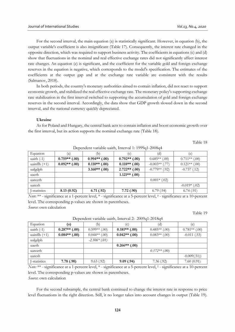
For the second interval, the main equation (a) is statistically significant. However, in equation (b), the

output variable's coefficient is also insignificant (Table 17). Consequently, the interest rate changed in the

opposite direction, which was required to support business activity. The coefficients in equations (c) and (d)

show that fluctuations in the nominal and real effective exchange rates did not significantly affect interest

rate changes. An equation (e) is significant, and the coefficient for the variable gold and foreign exchange

reserves in the equation is negative, which corresponds to the model's specification. The estimates of the

coefficients at the output gap and at the exchange rate variable are consistent with the results

(Salmanov, 2018).

In both periods, the country's monetary authorities aimed to contain inflation, did not react to support

economic growth, and stabilized the real effective exchange rate. The monetary policy's supporting exchange

rate stabilization in the first interval switched to supporting the accumulation of gold and foreign exchange

reserves in the second interval. Accordingly, the data show that GDP growth slowed down in the second

interval, and the national currency quickly depreciated.

Ukraine

As for Poland and Hungary, the central bank acts to contain inflation and boost economic growth over

the first interval, but its action supports the nominal exchange rate (Table 18).

Table 18

Dependent variable uairh, Interval 1: 1999q1-2008q4


uairh (-1) 0.759** (.00) 0.994** (.00) 0.792** (.00) 0.685** (.00) 0.711** (.00)

uainflh (+1) 0.092** (.00) 0.110** (.00) 0.118** (.00) -0.003** (.77) 0.121** (.00)

ualgdph 3.160** (.00) 2.722** (.00) -0.779** (.92) -0.737 (.12)

uaerh 1.121** (.00)

uareerh 0.001* (.02)

uaresh -0.019* (.02)

J-statistics 8.13 (0.92) 6.71 (.92) 7.72 (.90) 6.79 (.94) 6.74 (.91)




Table 19

Dependent variable uairh, Interval 2: 2009q1-2018q4


uairh (-1) 0.287** (.00) 0.599** (.00) 0.181** (.00) 0.485** (.00) 0.781** (.00)

uainflh (+1) 0.084** (.00) 0.044** (.00) 0.042** (.00) 0.083** (.00) -0.011 (.53)

ualgdph -2.506* (.01)

uaerh 0.266** (.00)

uareerh 0.172** (.00)

uaresh -0.009(.51))

J-statistics 7.78 (.90) 9.63 (.92) 9.09 (.94) 7.36 (.92) 7.60 (0.91)




For the second subsample, the central bank continued to change the interest rate in response to price

level fluctuations in the right direction. Still, it no longer takes into account changes in output (Table 19).



125

This conclusion is consistent with Kozmenko et al. (2014), who analyzed the Taylor rule on quarterly data

from 2004-2013 and found that the output gap did not significantly affect the National Bank of Ukraine's

interest rates. The unit root hypothesis is not rejected for the exchange rate variable uaerh (Table 1). Thus,

we can conclude that the monetary policy's main goal was to support price stability because of the country's

political events in the second interval.

5. CONCLUSION

In Eastern Europe and post-Soviet countries, monetary authorities directly or indirectly adhered to

specific rules based on interest rates as an instrument of monetary policy. In this study, monetary policy

rules' evolution reflects each country's changing priorities after the recent financial and economic crisis. We

performed an analysis of actual goals using quarterly data for two intervals: the first from 1998 to 2008 and

the second from 2009 to 2018 in nine transition economies of Eastern Europe and post-Soviet countries.

In practice, the research results provide a basis for identifying the actual goals, the achievement of which,

along with price stabilization, has been supported by monetary policy in each country.

The calculations showed that monetary authorities in all the countries under consideration contained

price growth as their priority goal throughout the entire interval. Moreover, the monetary authorities of the

countries chose alternative goals differently in each interval. The purpose of monetary policy was to support

economic growth in Hungary, Poland, and Ukraine only in the first interval. In all other cases, the interest

rate reacted in the wrong direction, or its effect was insignificant.

Interest rate behavior contributed to stabilizing Russia's exchange rate in the first interval, in Hungary

and Kazakhstan in the second interval, and Romania and Ukraine at both intervals. Moreover, in Belarus

and Poland, on the contrary, interest rate reactions did not contribute to the stabilization of the exchange

rate in both the first and second intervals.

The monetary authorities of Belarus, Kazakhstan, and Romania generated interest rate responses to

fluctuations in the real effective exchange rate in the direction of its stabilization at both intervals. Wrong

interest rate responses in Hungary in the first interval have changed to correct responses in the second

interval, which helps stabilize the real effective exchange rate. On the other hand, in Ukraine, the interest

rate responses have destabilized the second interval's real effective exchange rate.

The accumulation of gold and foreign exchange reserves was one of the alternative monetary policy

objectives in Belarus, the Czech Republic, and Romania in the first interval and Russia in the second interval.

Note that the interest rate dynamics did not correspond to Hungary's goal in the second interval and Russia

in the first interval.

Thus, in all the countries under consideration, price stabilization was the primary goal of their monetary

policy. In each of the two intervals, monetary authorities followed their own alternative goals. Moreover,

countries changed their priorities from the first interval to the second interval due to the financial and

economic crisis. Overall, they began to less support economic growth and the accumulation of foreign

exchange reserves while strengthening attention to stabilizing the exchange rate and the real effective

exchange rate. Further research may include more EE and CIS countries and other approaches, such as

cointegration analysis and dynamic stochastic general equilibrium models.


Vol.13, No.4, 2020

126

REFERENCES

Arlt, J., & Mandel, M. (2014). The reaction function of three central banks of Visegrad Group. Prague Economic Papers,

3, 2014, 269-289. doi: 10.18267/j.pep.484.

Clarida, R., Gali, J., & Gertler, M. (1998). Monetary policy rules in practice: some international evidence. European

Economic Review, 42, 1033-1067. doi.org/10.1016/S0014-2921(98)00016-6.

Corbo, V. (2000). Monetary Policy in Latin America in the 90s. Working Papers 78, Central Bank of Chile. Retrieved from:

http://si2.bcentral.cl/public/pdf/documentos-trabajo/pdf/dtbc78.pdf.

Dabrowski, M. (2013). Monetary Policy Regimes in CIS Economies and Their Ability to Provide Price and Financial

Stability. BOFIT Discussion Paper 8. Retrieved from: doi: 10.2139/ssrn.2267354.

Drobyshevski, S.M., Kozlovskaya, A., Levchenko, D., Ponomarenko, S., Trunin, P., & Chetverikov, S. (2003).

Comparative analysis of monetary policy in transition economies. Scientific papers No 58. Institute for the Economy

in Transition. Retrieved from: https://www.iep.ru/ru/publikatcii/publication/210.html.

El-Hodiri, M., & Mukhamediyev, B. (2014). Monetary policy rules in some transition economies. Eurasian journal of

economics and finance, 2(3), 26-44. doi: 10.15604/ejef.2014.02.03.002.

Esanov, A., Merkl, C., & Souza, L.V. (2005). Monetary Policy Rules for Russia. Journal of Comparative Economics, 33(3),

484-499. doi: 10.1016/j.jce.2005.05.003.

Friedman, M. (1956). The quantity theory of money: a restatement. In: Friedman, M. (Ed.), Studies in the Quantity Theory

of Money. University of Chicago Press, Chicago. Retrieved from: doi.org/10.1057/9780230280854_35.

Frommel, M., & Schobert, F. (2006). Monetary Policy Rules in Central and Eastern Europe. Deutsche Bundesbank.

Discussion Paper 341. Retrieved from: http://diskussionspapiere.wiwi.uni-hannover.de/pdf_bib/dp-341.pdf.

Ghatak, S., & Moore, T. (2011). Monetary Policy Rules for Transition Economies: An Empirical Analysis. Review of

Development Economics, 15(4), 714-728. Retrieved from: http://hdl.handle.net/10.1111/j.1467-

9361.2011.00638.x.

IMF. International Monetary Fund. Retrieved from: www.imf.org.

Hansen L.P. (1982). Large Sample Properties of Generalized Method of Moment Estimators. Econometrica, 50, 1029-

1054. doi:10.2307/1912775.

Greene W.H. (2012). Econometric analysis (7th ed.). Boston: Pearson Education Limited.

Keynes, J. M. (1936). The General Theory of Employment, Interest and Money. London: Macmillan.

Jawadi, F., Sousa, R., & Mallick, S. (2014). Nonlinear Monetary Policy Reaction Functions in Large Emerging

Economies: The Case of Brazil and China. Applied Economics, 46(9), 973-984.

Doi:10.1080/00036846.2013.851774.

Kozmenko, S., Savchenko, T., & Piontkovska, Y. (2014). Development and application of the monetary rule for the

base interest rate of the National Bank of Ukraine. Banks and Bank Systems, 9(3), 50-58.

doi:10.21511/bbs.9(3).2014.01.

Leong, C.M., Puah, C.H., Lau, E., & Shazali, A.M. (2019). Asymmetric effects of exchange rate changes on the demand

for divisia money in Malaysia. Journal of International Studies, 12(4), 52-62. doi:10.14254/2071-8330.2019/12-4/4.

McCallum, B. (1993). Specification and Analysis of a Monetary Policy Rule for Japan. NBER Working Paper 4449.

Retrieved from: https://www.nber.org/papers/w4449.pdf.

Mera, V., & Pop-Silaghi, M. (2015). An Insight Regarding Economic Growth and Monetary Policy in Romania. Scientific

Annals of Economics and Business, 62(1), 85-95. doi: 10.1515/aicue-2015-0039.

Mohanty, M.S., & Klau, M. (2005). Monetary Policy Rules in Emerging Market Economies: Issues and Evidence. In:

R.J. Langhammer, & L.V. de Souza. Monetary Policy and Macroeconomic Stabilization in Latin America. (pp.205-245)

Berlin, Heidelberg: Springer. Retrieved from: doi.org/10.1007/3-540-28201-7_13.

Mukhamediyev, B. (2007). Monetary policy rules of the National Bank of Kazakhstan. Quantile, 3, 91–106. Retrieved

from: https://ideas.repec.org/a/qnt/quantl/y2007i3p91-106.html.

Owusu, B.K. (2020). Estimating Monetary Policy Reaction Functions: Comparison between the European Central

Bank and Swedish Central Bank. Journal of Economic Integration, 35(3), 396-425. doi: 10.11130/jei.2020.35.3.396.

Papadamou, S., Sidiropoulos, M., & Vidra, A.A. (2018). Taylor Rule for EU members. Does one rule fit to all EU

member needs? The Journal of Economic Asymmetries, 18, e00104.



127

Popescu, I.V. (2014). Analysis of the Behavior of Central Banks in Setting Interest Rates. The Case of Central and

Eastern European Countries. Emerging Markets Queries in Finance and Business, 15, 1113-1121. doi: 10.1016/S2212-

5671(14)00565-6.

Redo, M., & Siemiątkowski, P. (2019). Cost channel in the mechanism of transmitting monetary policy in Poland.

Journal of International Studies, 12(4), 130-143. doi:10.14254/2071-8330.2019/12-4/9.

Salmanov, O.N., Babina, N.V., Ovsiychuk, V.Y., Drachena, I.P., & Vikulina, E.V. (2018). Analysis of the monetary

policy rule in the Russian economy. Journal of Social Sciences Research, (3), 304-312. doi: 10.32861/jssr.spi3.304.312.

Shkolnyk, I., Kozmenko, S., Kozmenko, O., & Mershchii, O. (2019). The impact of the economy financialization on

the level of economic development of the associate EU member states. Economics and Sociology, 12(4), 43-58.

doi:10.14254/2071-789X.2019/12-4/2.

Trung, T.B., & Kiss, G.D. (2020). Asymmetry in the Reaction Function of Monetary Policy in Emerging Economies.

Public Finance Quarterly-Hungary, 2(65), 210-224. doi:10.35551/PFQ_2020_2_4.

Vdovichenko, A.G., & Voronina, V.G. (2006). Monetary policy rules and their application in Russia. Research in

International Business and Finance, 20, 145–162. doi:10.1016/j.ribaf.2005.09.003.

Assessing hybrid monetary function reactions in transition ...

Documents

Transcript of Assessing hybrid monetary function reactions in transition ...