Aspects topologiques des flots en dimension 3 ......(P5) The dynamics of generic Kuperberg flows....
57
Aspects topologiques des flots en dimension 3 —– Topological aspects of flows on 3 dimensions Ana Rechtman 11 septembre 2017
Transcript of Aspects topologiques des flots en dimension 3 ......(P5) The dynamics of generic Kuperberg flows....
Aspects topologiques des flots en dimension 3
—–
Topological aspects of flows on 3 dimensions
Ana Rechtman
11 septembre 2017

Para Ema, como todo.
Table des matieres
Travaux de recherche 7
Introduction 9
1 A minimal set 131.1 The Seifert conjecture . . . . . . . . . . . . . . . . . . . . . . . . . . . . . . . . . . 141.2 Kuperberg’s construction and previous results . . . . . . . . . . . . . . . . . . . . . 15
1.2.1 The Kuperberg plug K . . . . . . . . . . . . . . . . . . . . . . . . . . . . . . 171.2.2 Notation and basic results on the dynamics . . . . . . . . . . . . . . . . . . 20
1.3 The minimal set under the generic hypotheses . . . . . . . . . . . . . . . . . . . . . 221.3.1 The special orbits . . . . . . . . . . . . . . . . . . . . . . . . . . . . . . . . 221.3.2 M0, a dense subset of the minimal set . . . . . . . . . . . . . . . . . . . . . 28
1.4 Pseudogroups . . . . . . . . . . . . . . . . . . . . . . . . . . . . . . . . . . . . . . . 311.4.1 Shape of the minimal set . . . . . . . . . . . . . . . . . . . . . . . . . . . . 351.4.2 Entropy of the minimal set . . . . . . . . . . . . . . . . . . . . . . . . . . . 37
1.5 Variations of the Kuperberg plug . . . . . . . . . . . . . . . . . . . . . . . . . . . . 391.6 Generic hypotheses . . . . . . . . . . . . . . . . . . . . . . . . . . . . . . . . . . . . 42
2 Trunkenness, an asymptotic invariant for flows 472.1 Independence of helicity . . . . . . . . . . . . . . . . . . . . . . . . . . . . . . . . . 52
Bibliography 55
3

4 TABLE DES MATIERES

Table des figures
1.1 A plug trapping a periodic orbit . . . . . . . . . . . . . . . . . . . . . . . . . . . . 141.2 Vector field Wv . . . . . . . . . . . . . . . . . . . . . . . . . . . . . . . . . . . . . 161.3 W-orbits on the cylinders r = cst. . . . . . . . . . . . . . . . . . . . . . . . . . . 161.4 W-orbits in the cylinder r = 2 . . . . . . . . . . . . . . . . . . . . . . . . . . . . 171.5 Embedding of Wilson Plug W as a folded figure-eight . . . . . . . . . . . . . . . . 171.6 The disks L1 and L2 . . . . . . . . . . . . . . . . . . . . . . . . . . . . . . . . . . . 181.7 The image of D1 under σ1 . . . . . . . . . . . . . . . . . . . . . . . . . . . . . . . 191.8 The radius inequality . . . . . . . . . . . . . . . . . . . . . . . . . . . . . . . . . . 191.9 The Kuperberg Plug K . . . . . . . . . . . . . . . . . . . . . . . . . . . . . . . . . 201.10 W with some Wilson arcs . . . . . . . . . . . . . . . . . . . . . . . . . . . . . . . . 211.11 The cylinder r = 2 in W′ . . . . . . . . . . . . . . . . . . . . . . . . . . . . . . . 231.12 The intersection of the orbit of p′(1; 1, 1) with the cylinder r = r1 . . . . . . . . 241.13 The intersection of the orbit of p′(1; 1, 2) with the cylinder r = r2 . . . . . . . . 251.14 The intersection of the orbit of p′(1; 1, 2; 1, 1) with the cylinder r = r2,1 . . . . . 251.15 Level 0 and 1 of S1 with gaps . . . . . . . . . . . . . . . . . . . . . . . . . . . . . 261.16 Level 0, 1 and 2 of S1 with gaps . . . . . . . . . . . . . . . . . . . . . . . . . . . . 271.17 The tree diagram for S1 with marked tips . . . . . . . . . . . . . . . . . . . . . . . 281.18 Finite propeller inside W . . . . . . . . . . . . . . . . . . . . . . . . . . . . . . . . 291.19 R′ ⊂W . . . . . . . . . . . . . . . . . . . . . . . . . . . . . . . . . . . . . . . . . . 291.20 τ(R′) ⊂ K . . . . . . . . . . . . . . . . . . . . . . . . . . . . . . . . . . . . . . . . 301.21 γ′ in L−1 . . . . . . . . . . . . . . . . . . . . . . . . . . . . . . . . . . . . . . . . . 301.22 Flattened M1
0 . . . . . . . . . . . . . . . . . . . . . . . . . . . . . . . . . . . . . . 301.23 Curves in τ(P ′γ) ∩ E1 . . . . . . . . . . . . . . . . . . . . . . . . . . . . . . . . . . 311.24 Flattened M0 . . . . . . . . . . . . . . . . . . . . . . . . . . . . . . . . . . . . . . 321.25 A rectangle R0 in the Kuperberg Plug K . . . . . . . . . . . . . . . . . . . . . . . 321.26 Domains and ranges for the maps φ+
1 , φ+2 , φ
−1 , φ
−2 . . . . . . . . . . . . . . . . . . 34
1.27 A pseudo-orbit as generator of the homology of the shape approximation . . . . . 361.28 The modified radius inequality for the cases ε < 0, ε = 0 and ε > 0 . . . . . . . . . 40
2.1 The trunk of the trefoil knot . . . . . . . . . . . . . . . . . . . . . . . . . . . . . . 49
5

6 TABLE DES FIGURES

Travaux de recherche
Je presente ici mes travaux de recherche, dans l’ordre chronologique. Je commence avec les deuxpapiers qui presentent les resultats de ma these.
(P1) Existence of periodic orbits for geodesible vector fields on closed3-manifolds. Ergodic Theory and Dynamical Systems 30, no. 6, 1817 - 1841,2010.
(P2) Minimal Følner foliations are amenable. En collaboration avec FernandoAlcalde Cuesta. Discrete and Continuous Dynamical Systems - Series A, Vol. 31,no. 3, 2011.
Le papier (P1) correspond a la premiere partie de ma these dediee a la question de l’existenced’orbites periodiques pour les flots geodesibles. J’ai montre leur existence sous certaines hypothesessupplementaires. Dans les preuves, j’utilise la technique des courbes pseudoholomorphes due a Hofer[Hof93]. Apres ma these, Klaus Niederkruger et moi avons utilise cette technique pour montrerl’existence d’orbites periodiques pour les flots de Reeb en dimension plus grande que 3, sous lapresence de sous-varietes feuilletees par la structure de contact. Le resultat fait l’objet du papier :
(P3) The Weinstein conjecture in the presence of submanifolds having aLegendrian foliation. En collaboration avec Klaus Niederkruger. Journal ofTopology and Analysis, Volume 3, Issue 4, 405-421, 2011.
Le papier (P2) correspond a la deuxieme (et derniere) partie de ma these, il s’agit d’etudier deuxpropietes de moyennabilite pour des feuilletages (ou pour les pseudogroupes). Une condition estlocale (c’est la condition dite de Følner) et l’autre est globale. Mes resultats on ete ameliores lors dema collaboration avec Fernando Alcalde Cuesta. Nous avons ecrit un deuxieme papier ensemble :
(P4) Averaging sequences. En collaboration avec Fernando Alcalde Cuesta. PacificJournal of Mathematics, Vol. 255, No. 1, 1-23, 2012.
Voici la liste de mes autres travaux :(P5) The dynamics of generic Kuperberg flows. En collaboration avec Steve
Hurder. Asterisque, Vol. 377, 1-250, 2016.
(P6) Two proofs of Taubes’ theorem on strictly ergodic flows. En colla-boration avec Victor Kleptsyn. A paraıtre dans les memoires de la conferenceII Reunion de Matematicos Mexicanos en el Mundo (MMM2014).
(P7) Aperiodicity at the boundary of chaos. En collaboration avec SteveHurder. A paraıtre dans Ergodic Theory and Dynamical Systems.
(P8) Equivalence of Deterministic walks on regular lattices on the plane.En collaboration avec Raul Rechtman. Physica A, Vol. 466, 69 - 78, 2017.
7
8 Travaux de recherche
(P9) The trunkenness of a volume-preserving vector field. En collaborationavec Pierre Dehornoy. A paraıtre dans Nonlinearity.
(P10) Perspectives on Kuperberg flows. En collaboration avec Steve Hurder.A paraıtre dans les memoires de la conference 31st Summer Conference on Topo-logy and its Applications.
Dans ce texte je presente des resultats tires des papiers (P5), (P7) et (P9). Le papier (P10) estune compilation de questions autour des flots de Kuperberg, il est cite dans ce texte.
Je vais donc utiliser quelques lignes pour vous raconter les resultats des articles (P6) et (P8),avant d’introduire mon memoire. Dans (P6) nous avons trouve deux preuves alternatives de l’enoncesuivant, qui a ete originalement prouve par C. H. Taubes [Tau09] en utilisant des invariants deSeiberg-Witten. Nous disons qu’un champ de vecteurs est strictement ergodique si son flot admetune unique mesure invariante et si cette mesure est un volume.
THEOREME. Soit X un champ de vecteurs sur S3 strictement ergodique. Alors l’helicite de Xest nulle.
L’helicite est definie dans la Section 2.1, il s’agit d’un invariant de conjugaison pour les flotsqui preservent un volume.
Dans l’article (P8) nous etablissons une equivalence entre deux modeles discrets de propagationde gaz dans un reseaux, appeles en anglais Lorenz lattice gases. Ils ont des proprietes remarquables.Notre papier donne une recette pour passer d’un modele a un autre sur des reseaux reguliers duplan.
Tous mes papiers peuvent etre consultes dans ma page web :
www.matem.unam.mx/rechtman/publications.html

Introduction
Dans ce memoire je presente des resultats relies a l’etude des flots en dimension 3. Le memoireest divise en deux chapitres. Le premier est dedie a mon travail pour comprendre l’ensemble minimaldu piege de Kuperberg, ou dit d’une autre facon, l’ensemble minimal des seules exemples connus deflots lisses sans points fixes et sans orbites periodiques sur S3. Dans le second, j’explique commentconstruire une quantite appelee tronc associee a un flot sur S3 muni d’une mesure invariante, qui estpreservee par conjugaison topologique. Ce resultat s’inscrit dans la demarche consistant a trouverdes invariants pour les flots provenant d’invariants pour les nœuds.
Les resultats presentes dans le premier chapitre ont ete obtenus en collaboration avec SteveHurder, avec qui j’ai commence a collaborer lors de mon postdoctorat a Chicago. Nous noussommes donne la tache de comprendre l’ensemble minimal du piege de Kuperberg. La premiereobservation importante pour ce faire est que la construction depend de certains choix, je citeE. Ghys [Ghys95] :
Par ailleurs, on peut construire beaucoup de pieges de Kuperberget il n’est pas clair qu’ils aient la meme dynamique.
Les choix donnent toujours un piege dont le flot est C∞, sans orbites periodiques et avec ununique ensemble minimal, mais nous ne savons pas si l’ensemble minimal est le meme pour tousles choix possibles. En effet, une question qui reste ouverte est de savoir s’il y a des choix pourlesquels l’ensemble minimal est de dimension 1. Dans notre travail, nous imposons des hypothesessupplementaires a la construction du piege qui nous permettent de montrer que l’ensemble minimalest de dimension topologique 2 et d’en deduire d’autres propietes dynamiques du flot. Nous appelonsces choix generiques, car il s’agit de demander que deux propietes de la construction soient denature quadratique. Nous appelons les flots obtenus des flots de Kuperberg generiques. Je presenteces hypotheses brievement dans la remarque 1.2.1 et avec plus de details dans la section 1.6.
Il faut mentionner que dans la categorie des flots lineaires par morceaux, Greg et Krystyna Ku-perberg parviennent a construire un piege de Kuperberg dont l’ensemble minimal est de dimension1 [KK96]. Aussi, si un piege de Kuperberg est tel que son ensemble minimal est de dimension 1,l’ensemble minimal est contenu dans un esemble invariant de dimension topologique 2 qui a lameme structure que l’ensemble minimal du cas generique.
Comment etudier un ensemble minimal ? Quels sont les aspects importants ?Une premiere approche est de se faire une image de cet ensemble minimal, de le visualiser.
Finalement c’est un ensemble plonge dans R3 et 3 est encore une petite dimension. J’ai essayedans ce memoire d’expliquer l’image que nous nous sommes faite de cet ensemble, la section 1.3.2donne une facon de comprendre comment il est structure. Tout n’y est pas dit, j’ai decide de ne pasrentrer dans certaines complications et details. Il s’agit donc d’une image idealisee de l’ensemble,qui permet de comprendre les autres aspects que nous avons decide d’etudier.
Une seconde approche naturelle est la theorie de la forme. Introduite par Borsuk [Bor68], ellepermet d’etudier certains aspects des ensembles plonges dans un espace euclidien, en etudiant des
9
10 Introduction
suites de voisinages de plus en plus petits. Nous avons ete guides par une question de K. Kuperberg :est ce que la forme de l’ensemble minimal est stable ? Comme explique dans la section 1.4.1, noussavons que la reponse a cette question est negative (dans le cas d’un flot de Kuperberg generique).Le concept d’ensemble «movable» est un autre concept important dans la theorie de la forme. Nousignorons si l’ensemble minimal des flots de Kuperberg generiques est «movable». Je conjecture queoui.
Nous comprenons donc comment visualiser cet ensemble minimal exceptionnel (c’est-a-diretransversement un ensemble de Cantor) de dimension topologique 2. Il est, par minimalite, locale-ment homogene, mais il n’est pas globalement homogene. Comme explique dans le theoreme 1.3.5,l’ensemble ne forme pas une lamination, mais il contient un ouvert dense de dimension 2 qui estune lamination L avec des feuilles ouvertes. Nous pouvons donc considerer la dynamique de cettelamination et la comparer a la dynamique du flot restreint a l’ensemble minimal.
Cet approche nous a permis de construire des pseudogroupes agissant, soit dans un rectanglepresque transverse au flot, soit dans une transversale a la lamination L. Il s’agit, par leur nature etpar la construction, de pseudogroupes differents mais semblables, avec des ensembles de generateurssimilaires. Le premier de ces pseudogroupes est decrit brievement dans la section 1.4. En utilisantla notion d’entropie pour les pseudogroupes, introduite par Ghys, Langevin et Walczak [GLW88],nous avons etudie ces pseudogroupes. Dans la section 1.4.2, j’explique quelques-uns des resultatobtenus.
Les pseudogroupes utilises dans [P5] ont tous la propiete que le nombre de points separes pardes mots de longueur n (avec un ensemble de generateurs fixe) croıt comme l’exponentielle denα, pour un certain α ∈ (0, 1). Ils sont donc tous d’entropie nulle, mais d’entropie lente positive(les definitions sont donnees dans la section 1.4.2). Cette affirmation s’etend au flot restreint al’ensemble minimal : le flot est d’entropie topologique nulle, mais a une entropie lente positive. Lefait que l’entropie topologique du flot soit nulle est aussi une consequence d’un theoreme de Katok[Kat80], comme remarque par E. Ghys [Ghys95].
Avec l’objectif de trouver de flots a entropie topologique positive pres des flots de Kuperberg,nous avons etudie des deformations de la construction du piege dans [P7]. Nous avons donc trouveune famille C∞ a un parametre contenant un flot de Kuperberg et des flots a entropie positive. Laconstruction et quelques idees des preuves forment le contenu de la section 1.5.
Le flot de Kuperberg est donc une bifurcation dans l’espace des flots sur une variete fermee dedimension 3. Il s’agit d’une situation non generique, mais ce flot doit probablement etre entoured’autres bifurcations parmi lesquelles il pourrait y avoir des bifurcations generiques. Je ne sais pasen ce moment, si l’etude d’un voisinage du piege parmi les bifurcations est abordable.
Par ailleurs, les pieges a entropie topologique positive construites dans [P7] contiennent unefamille denombrable d’ensembles invariants dont la dynamique transverse est conjuguee a un fer acheval. Comment ceux-ci degenerent-ils vers l’ensemble minimal du piege de Kuperberg ? Le tempsde retour a ces ensembles tranverses invariants devient de plus en plus long quand on s’approchedu piege de Kuperberg, mais j’ignore si c’est l’unique cause de la bifurcation. Il me semble doncinteressant de comprendre ce processus.
Les resultats du deuxieme chapitre ont ete obtenus en collaboration avec Pierre Dehornoy. Nousavons construit une quantite associee a un champ de vecteursX muni d’une mesure invariante µ, quiest preservee par conjugaison. Nous appelons cette quantite un invariant de (X,µ). Ce probleme estmotive par une observation de Helmholtz [Hel1858] : si Xt est un champ de vecteurs non-autonomequi satisfait les equations d’Euler (dans le cas plus simple de ces equations) et si on note φt sonflot, alors rot(Xt) est l’image sous φt de rot(X0). Comme φt est un diffeomorphisme qui preserve

Introduction 11
un volume, un invariant applique a rot(X0) nous donne une quantite qui ne depend pas du tempspour les solutions de l’equation d’Euler.
L’invariant le plus connu est l’helicite, il est defini quand la mesure invariante µ est un volume.Grace aux travaux d’Arnold [Arn73], nous avons une interpretation topologique de cet invariant :dans S3 (ou un domaine simplement connexe de R3), l’helicite coıncide avec le nombre d’enlacementasymptotique. Ce nombre est defini de la facon suivante. Prenons deux points x1, x2 ∈ S3 et deuxnombres t1, t2 ∈ R. On considere les courbes k(xi, ti), pour i = 1, 2, formees par le segmentd’orbite entre xi et φti(xi) suivi d’un arc (court) entre ces deux points. On peut montrer [Vog02]que pour presque toute paire de points et pour presque toute paire de nombres reels, on obtientdeux courbes fermees simples et disjointes. Nous pouvons donc calculer leur nombre d’enlacement`(k(x1, t1), k(x2, t2)). L’helicite est alors egale a∫ ∫ (
limt1,t2→∞
`(k(x1, t1), k(x2, t2))t1t2
)dµdµ.
Si µ est une mesure ergodique, nous n’avons pas besoin d’integrer. Cette interpretation nous dit quel’helicite est un invariant asymptotique : elle peut etre obtenue comme la limite d’un invariant desentrelacs. Il semble donc naturel d’imiter cettte construction pour d’autres invariants de nœuds ouentrelacs, pour trouver d’autres invariants asymptotiques. Cette voie a ete exploree par Gambaudoet Ghys [GG01], Baader [Baa11] et Baader et Marche [BM12], pour differents invariants des nœuds.Mais tous les invariants obtenus par ces auteurs sont proportionnels a l’helicite.
Recemment, Kudryavtseva [Kud14, Kud16] et Enciso, Peralta-Salas et Torres de Lizaur [EPT16]ont montre sous differentes hypotheses, que tout invariant dont la derivee de Frechet est l’integraled’un noyau continu, est une fonction de l’helicite. Donc, si l’on cherche de nouveaux invariants, ilsne peuvent pas etre trop reguliers.
Nous avons decide d’etudier un invariant des nœuds appele le tronc, introduit par Ozawa[Ozw10]. Cet invariant est construit en comptant le nombre de points d’intersections entre unnœud et les niveaux d’une fonction hauteur. Dans le cas de S3, une fonction hauteur a deux pointssinguliers et tout autre niveau est une sphere. Une adaptation naturelle au cas des champs devecteurs est le flux geometrique a travers les niveaux de la fonction. Il s’agit de mesurer par rapporta une mesure invariante, le passage infinitesimal a travers la surface sans considerer l’orientation.
L’invariant qui en resulte, est un invariant par conjugaison topologique, et il admet une in-terpretation asymptotique : dans le cas d’une mesure ergodique, il s’agit de la limite du tronc dek(x, t) divise par t, pour presque tout x ∈ S3. Je presente dans le chapitre 2 les resultats quenous avons obtenus concernant cet invariant, en particulier, nous pouvons montrer qu’il n’est pasproportionnel a l’helicite. Dans la section 2.1, j’ai decide d’inclure le calcul qui nous permet demontrer cette derniere affirmation.

12 Introduction
Chapter 1
A minimal set
A 3-dimensional closed manifold has Euler characteristic zero, meaning that it admits a non-singular vector field. There is one known way to build C∞ or real analytic flows without fixedpoints and without periodic orbits that applies to any of these manifolds: using Kuperberg plugs. Aplug allows to modify a flow inside a flow-box, trapping orbits and introducing at least a minimalset.
K. Kuperberg’s construction appeared in 1993, published in 1994 [Kup94]. The article wasthen followed by a Seminaire Bourbaki exposition by E. Ghys [Ghys95], a Sugaku lecture by S.Matsumoto [Mat95] and a paper by Greg and Krystyna Kuperberg [KK96]. Each of these papersgives different insights into the dynamics of Kuperberg flows, I will explain briefly some of themin Section 1.2.2. Regarding the minimal set of the flow inside the plug, it was known that there isonly one minimal set.
In [P5], S. Hurder and I went into the details of these flows, trying to understand what theminimal set looks like. I will give here an informal description of it and cite the main results ofour work, mainly related to its shape properties and some types of entropy of the flow. To myknowledge, our work gives the first explicit example of an exceptional minimal set of a flow thathas topological dimension 2 and is not obtained from a suspension of a diffeomorphism. Thisminimal set has amazing properties, some of them explained below. We developed a set of ad-hoctechniques for studying it. I ignore if any of these can be applied to other minimal sets.
The chapter is organized as follows. Sections 1.1 and 1.2 are a brief introduction to the problemand the results on Kuperberg flows previous to our work. Section 1.2 is divided into the originalconstruction by K. Kuperberg explained in Section 1.2.1 and some known results on their dynamicsother than aperiodicity explained in Section 1.2.2. In Section 1.3.2 and its subsections, I tried togive a picture of the minimal set. In Section 1.3.1, I start by explaining the structure of two specialorbits of the flow, then in Section 1.3.2 I use these two orbits to decompose a dense subset of theminimal set whose dimension is 2. This is not a formal exposition since it avoids several minorcomplications and I refer for the proofs of the facts used to [P5].
In the paper [P5] we used several pseudogroups acting on a rectangle that is almost transverseto the flow of the Kuperberg plug to study the dynamics beyond aperiodicity. Even if in this textI don’t present any proof using pseudogroups, I included in Section 1.4 the rectangle and some ofthe maps we studied in [P5]. These maps then appear in the discussions in Sections 1.4.2 and 1.5.
Section 1.5 corresponds to the results obtained in [P7]. Kuperberg flows have topological en-tropy zero, as a consequence of Katok’s theorem on C2-flows [Kat80]. The question that motivatedthe results in [P7] was if there are positive topological entropy flows arbitrarily near the Kuper-berg flows. The answer is yes in the C1-topology by more general results on 3-dimensional flows.Since the Kuperberg examples are explicit, it seemed that we could work in the C∞-topology.
13

14 CHAPTER 1. A MINIMAL SET
The answer is again yes: we found an explicit construction of a 1-parameter family containing aKuperberg flow and flows of positive topological entropy. I give the construction highlighting thedifference with the original construction by K. Kuperberg and explain the main ideas in the proof.
1.1 The Seifert conjecture, a story beyond Wilson, Schweitzerand Kuperberg
In 1950, Seifert proved that vector fields close to a vector field tangent to the Hopf fibrationhave periodic orbits. He asked if any non-singular vector field on the three sphere S3 had a periodicorbit, the positive answer to this question became known as the Seifert conjecture.
Some years later, in 1966, F. W. Wilson built a plug that allows to obtain on any closed3-manifold a non-singular vector field with a finite number of periodic orbits [Wil66, PW77] (theconstruction in the second paper is simpler). At this point, the problem was how to destroy thoseperiodic orbits and there was a possible path: to build a plug without periodic orbits.
To fix ideas, let me define a plug. A 3-dimensional plug is a manifold P endowed with a vectorfield X satisfying the following properties: the manifold P is of the form D × [−2, 2], where D isa compact 2-manifold with boundary ∂D. Let ∂
∂z be the vertical vector field on P , where z is thecoordinate on [−2, 2]. The vector field X on P must satisfy the conditions:
(P1) vertical near the boundary: X = ∂∂z in a neighborhood of ∂P ; thus, D×−2 and D×2
are the entry and exit regions of P for the flow of X , respectively;(P2) entry-exit condition: if a point (x,−2) is in the same trajectory as (y, 2), then x = y.
That is, an orbit that traverses P , exits just in front of its entry point;(P3) trapped orbit: there is at least one entry point whose entire forward orbit is contained in
P ; we will say that its orbit is trapped by P and we call the set of entry point with trappedorbit the trapped set;
(P4) tameness: there is an embedding i : P → R3 that preserves the vertical direction on theboundary ∂P .
A plug is aperiodic if there is no closed orbit for X . After Wilson’s result an aperiodic plug will
Figure 1.1: A plug trapping a periodic orbit
allow to build a vector field without periodicorbits. Indeed, we can use such a plug to de-stroy the periodic orbits one by one. Considerone periodic orbit, it suffices to embed the ape-riodic plug in a flow-box intersecting the peri-odic orbit in such a way that the periodic orbitgets trapped inside the plug, thus it will nolonger be periodic. This can be done by con-ditions (P1), (P3) and (P4). Condition (P2)guarantees that there are no new periodic or-bits after surgery: there are no periodic orbitsinside the plug and if an orbit intersects theplug and is not trapped, the entry-exit condi-tion implies that it will stay periodic or non-periodic after surgery. Repeating this processat most finitely many times, gives an aperiodicflow on any closed 3-manifold.
The first aperiodic plug was built by P. Schweitzer [Sch74] in 1974, though the flow is only C1.The aperiodic plug that is C∞ (an even real analytic) was built by K. Kuperberg in 1993 [Kup94].Notice that almost 20 years passed between the two constructions, in the meantime J. Harrison

1.2. KUPERBERG’S CONSTRUCTION AND PREVIOUS RESULTS 15
managed to make a C2 version of Schweitzer’s plug [Har88] and there are a couple of papers tryingto prove that it is impossible to build an aperiodic plug with a smooth flow. But how to provethat there are no aperiodic plugs in the Cr category for r > 2?
Let me highlight one of the main differences between Schweitzer’s and Kuperberg’s construction.Condition (P3) in the definition of a plug implies that a trapped orbit has to accumulate on aninvariant set, thus a plug contains a minimal set for the flow. Schweitzer’s construction startswith a minimal set: the main idea is to substitute the periodic orbits in the Wilson plug with twocopies of the Denjoy minimal set. The differentiability problem comes from this set. J. Harrisonchanged the embedding of the minimal set to make the flow C2. Kuperberg’s construction focuseson destroying the periodic orbits of the Wilson plug, there is some minimal set in the plug, but nottoo much was known about it before our work. I will cite Matsumoto to describe K. Kuperberg’sconstruction:
We therefore must demolish the two closed orbits in the Wilson Plug beforehand.But producing a new plug will take us back to the starting line. The idea of Kuperbergis to let closed orbits demolish themselves. We set up a trap within enemy lines andwatch them settle their dispute while we take no active part.
After Schweitzer’s construction the idea to prove that it was impossible to build a C∞ aperiodicplug focuses on the minimal set inside the plug (the starting point of his construction). I want tomention a paper by M. Handel [Han80], in which he proves that if the trapped orbits of a plugaccumulate on a minimal set whose dimension is 1 and this is the only invariant set for the flow inthe plug, then the minimal set is surface-like: the flow restricted to the minimal set is topologicallyconjugated to the minimal set of a flow on a surface. He considers also the case of a minimal setwhose topological dimension is two, but he makes the assumption that there is a disk-like sectionof the minimal set. In Kuperberg’s plug the minimal set is not the only invariant set of the plug,as proved by S. Matsumoto (see Theorem 1.2.3), and when it has topological dimension 2 it doesnot admits a disk-like section.
There is also a paper by R. J. Knill that embeds Denjoy minimal sets in C∞-flows on S3,but these are not isolated as any neighborhood contains periodic orbits [Kni81]. Hence, untilK. Kuperberg’s construction, the idea was to look at the possible minimal sets for an aperiodicplug.
It seems a good moment to comment on two (difficult) questions. The first one is on thedimension of the minimal set of the Kuperberg plug. We proved in [P5] that, under some extraassumptions on the construction, this set has topological dimension two. We do not know if thereare smooth Kuperberg flows whose minimal set has dimension 1. I have tried to build them withoutsuccess. Can one prove that a minimal set with dimension 1 and unstable shape cannot be isolated(meaning that any neighborhood should contain periodic orbits)? The answer to this question isyes if the minimal set is a solenoid as proved by E. S. Thomas [Tho73].
Secondly, consider the case of volume preserving flows on 3-manifolds. We are at the stage ofknowing that there are examples with a finite number of periodic orbits and C1 examples withoutperiodic orbits on any closed 3-manifold. These were built by G. Kuperberg [Kup96]. Is it possibleto build a C∞ volume preserving aperiodic plug? Can we a priori say something about its minimalor invariant sets?
1.2 Kuperberg’s construction and previous resultsAs mentioned above, K. Kuperberg’s idea is to destroy the periodic orbits in the modified
Wilson’s plug using the plug itself, or let the periodic orbits demolish themselves. So I start

16 CHAPTER 1. A MINIMAL SET
explaining how to build Wilson’s plug (actually a modified version of the original plug). Theconstruction of the self-insertions that destroy the periodic orbits is explained in Section 1.2.1.
Consider the rectangle
R = [1, 3]× [−2, 2] = (r, z) | 1 ≤ r ≤ 3 &− 2 ≤ z ≤ 2.
Choose a C∞-function g : R → [0, g0] for g0 > 0, which satisfies the “vertical” symmetry conditiong(r, z) = g(r,−z). Also, require that g(2,−1) = g(2, 1) = 0 and that g(r, z) > 0 otherwise. Definethe vector fieldWv = g· ∂∂z which has two singularities, (2,±1) and is otherwise everywhere vertical,as illustrated in Figure 1.2.
Figure 1.2: Vector field Wv
Next, choose a C∞-function f : R → [−1, 1]which satisfies the following conditions:
(W1) f(r,−z) = −f(r, z) [anti-symmetry in z].
(W2) f(ξ) = 0 for ξ near the boundary of R.
(W3) f(r, z) ≥ 0 for −2 ≤ z ≤ 0.
(W4) f(r, z) ≤ 0 for 0 ≤ z ≤ 2.
(W5) f(2,−1) = 1 and f(2, 1) = −1.
Next, define the manifold with boundary
W = [1, 3]× S1 × [−2, 2] ∼= R × S1 (1.1)
with cylindrical coordinates x = (r, θ, z). That is,W is a solid cylinder with an open core removed,obtained by rotating the rectangle R, considered asembedded in R3, around the z-axis.
Extend the functions f and g above to W bysetting f(r, θ, z) = f(r, z) and g(r, θ, z) = g(r, z), sothat they are invariant under rotations around the
z-axis. The modified Wilson vector field W on W is defined by
W = g(r, θ, z) ∂∂z
+ f(r, θ, z) ∂∂θ
. (1.2)
Let Ψt denote the flow of W on W. Observe that the vector field W is vertical near the boundaryof W, and is horizontal for the points (r, θ, z) = (2, θ,±1). Also, W is tangent to the cylindersr = cst.. The flow Ψt on the cylinders r = cst. is illustrated by Figure 1.3.
Figure 1.3: W-orbits on the cylinders r = cst.
1.2. KUPERBERG’S CONSTRUCTION AND PREVIOUS RESULTS 17
Define the closed subsets:
R ≡ (2, θ, z) | −1 ≤ z ≤ 1 [The Reeb Cylinder ]A ≡ z = 0 [The Center Annulus]Oi ≡ (2, θ, (−1)i) [Periodic Orbits, i=1,2 ]
∂−h W ≡ (r, θ,−2) [The Entry Region]∂+hW ≡ (r, θ, 2) [The Exit Region]
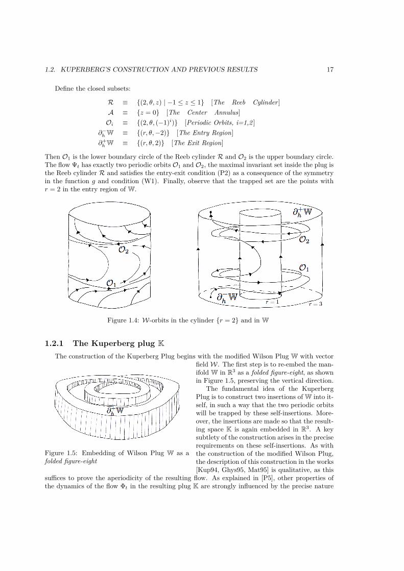
Then O1 is the lower boundary circle of the Reeb cylinder R and O2 is the upper boundary circle.The flow Ψt has exactly two periodic orbits O1 and O2, the maximal invariant set inside the plug isthe Reeb cylinder R and satisfies the entry-exit condition (P2) as a consequence of the symmetryin the function g and condition (W1). Finally, observe that the trapped set are the points withr = 2 in the entry region of W.
Figure 1.4: W-orbits in the cylinder r = 2 and in W
1.2.1 The Kuperberg plug KThe construction of the Kuperberg Plug begins with the modified Wilson Plug W with vector
Figure 1.5: Embedding of Wilson Plug W as afolded figure-eight
fieldW. The first step is to re-embed the man-ifold W in R3 as a folded figure-eight, as shownin Figure 1.5, preserving the vertical direction.
The fundamental idea of the KuperbergPlug is to construct two insertions of W into it-self, in such a way that the two periodic orbitswill be trapped by these self-insertions. More-over, the insertions are made so that the result-ing space K is again embedded in R3. A keysubtlety of the construction arises in the preciserequirements on these self-insertions. As withthe construction of the modified Wilson Plug,the description of this construction in the works[Kup94, Ghys95, Mat95] is qualitative, as this
suffices to prove the aperiodicity of the resulting flow. As explained in [P5], other properties ofthe dynamics of the flow Φt in the resulting plug K are strongly influenced by the precise nature

18 CHAPTER 1. A MINIMAL SET
of these maps, so some hypotheses were added to the construction. We call a plug satisfying thesehypotheses a generic Kuperberg plug. In Remark 1.2.1 at the end of this section I briefly explainthe generic hypotheses and in Section 1.6 I give a compilation of the generic hypotheses.
After the embedding presented in Figure 1.5, the construction continues with the choice in theannulus [1, 3] × S1 of two closed regions Li, for i = 1, 2, which are topological disks. Each regionhas boundary defined by two arcs: for i = 1, 2, α′i is the boundary contained in the interior of[1, 3]× S1 and αi in the outer boundary contained in the circle r = 3, as depicted in Figure 1.6.
Figure 1.6: The disks L1 and L2
Consider the closed sets Di ≡ Li× [−2, 2] ⊂W, for i = 1, 2. Note that each Di is homeo-morphic to a closed 3-ball, that D1 ∩ D2 = ∅and each Di intersects the cylinder r = 2 ina rectangle. Label the top and bottom faces ofthese regions by
L±1 = L1 × ±2 , L±2 = L2 × ±2 . (1.3)
The next step is to define insertion mapsσi : Di → W, for i = 1, 2, in such a waythat the periodic orbits Oi flow Ψt intersectσi(L−i ) in points corresponding to W-trappedentry points for the Wilson plug W. Considertwo disjoint arcs β′i in the inner boundary cir-cle r = 1, that are in front of the arcs αiwhen the plug is embedded as in Figure 1.5.
For i = 1, 2, choose orientation preserving diffeomorphisms σi : α′i → β′i and extend these maps tosmooth embeddings σi : Di →W, as illustrated in Figure 1.7, which satisfy the conditions:
(K1) σi(α′i × z) = β′i × z for z ∈ [−2, 2], the interior arc α′i is mapped to a boundary arc β′i;(K2) for Di = σi(Di), D1 ∩ D2 = ∅;(K3) σ1(L−1 ) ⊂ z < 0 and σ2(L+
2 ) ⊂ z > 0;(K4) For every x ∈ Li, the image σi(x× [−2, 2]) is an arc contained in a trajectory of W;(K5) Each slice σi(Li × z) is transverse to the vector field W, for all −2 ≤ z ≤ 2;(K6) Di intersects the periodic orbit Oi and not Oj , for i 6= j.For i = 1, 2, the components of the boundary of the embedded regions Di = σi(Di) ⊂ W that
are transverse to W are labeled byL±i = σi(L±i ) . (1.4)
Note that the arcs σi(x×[−2, 2]) in condition (K3) are line segments from σi(x×−2) ∈ L−i toσi(x×2) ∈ L+
i which follow theW-trajectory and traverse the insertion from the bottom face tothe top face. SinceW is vertical near the boundary of W and horizontal at the two periodic orbits,we have that the arcs σi(x× [−2, 2]) are vertical near the inserted curve σi(α′i) and horizontal atthe intersection of the insertion with the periodic orbit Oi. Thus, the embeddings of the surfacesσi(Li×z) make a half turn upon insertion, for each −2 ≤ z ≤ 2. The turning is clockwise for thebottom insertion i = 1 as illustrated in Figure 1.7 and counter-clockwise for the upper insertioni = 2, which is illustrated in Figure 1.9.
The embeddings σi are also required to satisfy two further conditions, which are the key toshowing that the resulting Kuperberg flow Φt is aperiodic:
(K7) For i = 1, 2, the disk Li contains a point (2, θi) such that the image under σi of thevertical segment (2, θi)× [−2, 2] ⊂ Di ⊂W is an arc of the periodic orbit Oi of W.
(K8) Radius Inequality: For all x = (r′, θ′, z′) ∈ Li × [−2, 2], let (r, θ, z) = σi(r′, θ′, z′) ∈ Di,then r′ > r unless x = (2, θi, z).

1.2. KUPERBERG’S CONSTRUCTION AND PREVIOUS RESULTS 19
Figure 1.7: The image of D1 under σ1
Figure 1.8: The radius inequality
The Radius Inequality (K8), illustrated inFigure 1.8, is one of the most fundamental con-cepts of Kuperberg’s construction. This is an“idealized” case, as it implicitly assumes thatthe relation between the values of r and r′ is“quadratic” in a neighborhood of the specialpoints (2, θi), which is not required in orderthat (K8) be satisfied. This “quadratic condi-tion” is part of the generic hypotheses on theconstruction (see Remark 1.2.1 and Hypothesis1.6.3).
The Radius Inequality (K8) is a monotonecondition that allows to keep track of the be-havior of the orbits in the Kuperberg plug. It isthis condition that is violated in the construc-tion in Section 1.5.
The embeddings σi : Li × [−2, 2] → W, fori = 1, 2, can be constructed by first choosingsmooth embeddings of the faces σi : L−i → Wso that the image surfaces are transverse to thevector field W on W and satisfy the conditions(K1), (K5) for z = −2, (K7) and (K8). Thenwe extend the embeddings of the faces L−i tothe sets Li × [−2, 2] by flowing the images us-ing a reparametrization of the flow of W, sothat we obtain embeddings of Li × [−2, 2] sat-isfying conditions (K1) to (K8), as pictured inFigure 1.7 for the bottom insertion.
Finally, define K to be the quotient man-ifold obtained from W by identifying the sets
Di with Di. That is, for each point x ∈ Di identify x with σi(x) ∈ W, for i = 1, 2, as illustratedin Figure 1.9. The restricted Ψt-flow on the inserted disk Di = σi(Di) is not compatible with theimage of the restricted Ψt-flow on Di. Thus it is necessary to modify W on each insertion Di,by replacing the vector field W on the interior of each region Di with the image vector field, sothat the dynamics in the interior of each insertion region Di reverts back to the Wilson dynamicson Di. As for the insertion of plugs, the flow has to be reparametrized near the boundary of theinsertion so that the resulting flow is C∞. Let K be the resulting vector field and Φt its flow.
REMARK 1.2.1 (The generic hypotheses). Under the name generic hypotheses, we added in[P5] a set of conditions to the constructions of the modified Wilson plug W and the Kuperbergplug K that allowed us to study the dynamics of the flows beyond aperiodicity. Some of these aretechnical assumptions, but they can be classified into two classes:
— The function g in the construction of the modified Wilson plug W is zero only at the points(2,±1) of the rectangle and the speed at which it goes to zero near this points is specified inthe generic hypotheses: we ask g to be a quadratic function of the distance to these points(in a small neighborhood).
— The Radius Inequality (K8) is required to be quadratic near the special points, as suggestedby Figure 1.8.
These assumptions are used to prove that the minimal set in the plug has topological dimension2 (see Chapter 17 of [P5]), to give explicit computations of the topological entropy of the flow
20 CHAPTER 1. A MINIMAL SET
Figure 1.9: The Kuperberg Plug K
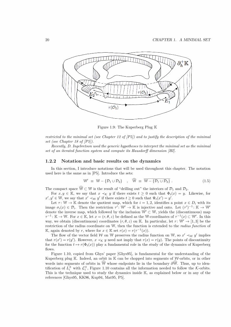
restricted to the minimal set (see Chapter 12 of [P5]) and to justify the description of the minimalset (see Chapter 18 of [P5]).
Recently, D. Ingebretson used the generic hypotheses to interpret the minimal set as the minimalset of an iterated function system and compute its Hausdorff dimension [HI].
1.2.2 Notation and basic results on the dynamicsIn this section, I introduce notations that will be used throughout this chapter. The notation
used here is the same as in [P5]. Introduce the sets:
W′ ≡ W− D1 ∪ D2 , W ≡ W− D1 ∪ D2 . (1.5)
The compact space W ⊂W is the result of “drilling out” the interiors of D1 and D2.For x, y ∈ K, we say that x ≺K y if there exists t ≥ 0 such that Φt(x) = y. Likewise, for
x′, y′ ∈W, we say that x′ ≺W y′ if there exists t ≥ 0 such that Ψt(x′) = y′.Let τ : W → K denote the quotient map, which for i = 1, 2, identifies a point x ∈ Di with its
image σi(x) ∈ Di. Then the restriction τ ′ : W′ → K is injective and onto. Let (τ ′)−1 : K → W′denote the inverse map, which followed by the inclusion W′ ⊂ W, yields the (discontinuous) mapτ−1 : K→W. For x ∈ K, let x = (r, θ, z) be defined as the W-coordinates of τ−1(x) ⊂W′. In thisway, we obtain (discontinuous) coordinates (r, θ, z) on K. In particular, let r : W′ → [1, 3] be therestriction of the radius coordinate on W, then the function is extended to the radius function ofK, again denoted by r, where for x ∈ K set r(x) = r(τ−1(x)).
The flow of the vector field W on W preserves the radius function on W, so x′ ≺W y′ impliesthat r(x′) = r(y′). However, x ≺K y need not imply that r(x) = r(y). The points of discontinuityfor the function t 7→ r(Φt(x)) play a fundamental role in the study of the dynamics of Kuperbergflows.
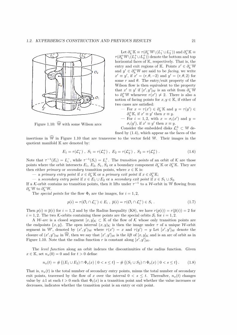
Figure 1.10, copied from Ghys’ paper [Ghys95], is fundamental for the understanding of theKuperberg plug K. Indeed, an orbit in K can be chopped into segments of W-orbits, or in otherwords into segments of orbits in W whose endpoints lie in the boundary ∂W. Thus, up to iden-tification of L±i with L±i , Figure 1.10 contains all the information needed to follow the K-orbits.This is the technique used to study the dynamics inside K, as explained below or in any of thereferences [Ghys95, KK96, Kup94, Mat95, P5].
1.2. KUPERBERG’S CONSTRUCTION AND PREVIOUS RESULTS 21
Figure 1.10: W with some Wilson arcs
Let ∂−h K ≡ τ(∂−h W\(L−1 ∪L
−2 )) and ∂+
h K ≡τ(∂+
hW\(L+1 ∪L
+2 )) denote the bottom and top
horizontal faces of K, respectively. That is, theentry and exit regions of K. Points x′ ∈ ∂−h Wand y′ ∈ ∂+
hW are said to be facing, we writex′ ≡ y′, if x′ = (r, θ,−2) and y′ = (r, θ, 2) forsome r and θ. The entry/exit property of theWilson flow is then equivalent to the propertythat x′ ≡ y′ if [x′, y′]W is an orbit from ∂−h Wto ∂+
hW whenever r(x′) 6= 2. There is also anotion of facing points for x, y ∈ K, if either oftwo cases are satisfied:
— For x = τ(x′) ∈ ∂−h K and y = τ(y′) ∈∂+h K, if x′ ≡ y′ then x ≡ y.
— For i = 1, 2, with x = σi(x′) and y =σi(y′), if x′ ≡ y′ then x ≡ y.
Consider the embedded disks L±i ⊂ W de-fined by (1.4), which appear as the faces of the
insertions in W in Figure 1.10 that are transverse to the vector field W. Their images in thequotient manifold K are denoted by:
E1 = τ(L−1 ) , S1 = τ(L+1 ) , E2 = τ(L−2 ) , S2 = τ(L+
2 ) . (1.6)
Note that τ−1(Ei) = L−i , while τ−1(Si) = L+i . The transition points of an orbit of K are those
points where the orbit intersects E1, E2, S1, S2 or a boundary component ∂−h K or ∂+h K. They are
then either primary or secondary transition points, where x ∈ K is:— a primary entry point if x ∈ ∂−h K or a primary exit point if x ∈ ∂+
h K;— a secondary entry point if x ∈ E1 ∪ E2 or a secondary exit point if x ∈ S1 ∪ S2.
If a K-orbit contains no transition points, then it lifts under τ−1 to a W-orbit in W flowing from∂−h W to ∂+
hW.The special points for the flow Φt are the images, for i = 1, 2,
p(i) = τ(Oi ∩ L−i ) ∈ Ei , p(i) = τ(Oi ∩ L+i ) ∈ Si . (1.7)
Then p(i) ≡ p(i) for i = 1, 2 and by the Radius Inequality (K8), we have r(p(i)) = r(p(i)) = 2 fori = 1, 2. The two K-orbits containing these points are the special orbits Si for i = 1, 2.
A W-arc is a closed segment [x, y]K ⊂ K of the flow of K whose only transition points arethe endpoints x, y. The open interval (x, y)K is then the image under τ of a unique W-orbitsegment in W′, denoted by (x′, y′)W where τ(x′) = x and τ(y′) = y Let [x′, y′]W denote theclosure of (x′, y′)W in W, then we say that [x′, y′]W is the lift of [x, y]K and is an arc of orbit as inFigure 1.10. Note that the radius function r is constant along [x′, y′]W .
The level function along an orbit indexes the discontinuities of the radius function. Givenx ∈ K, set nx(0) = 0 and for t > 0 define
nx(t) = # (E1 ∪ E2) ∩ Φs(x) | 0 < s ≤ t −# (S1 ∪ S2) ∩ Φs(x) | 0 < s ≤ t . (1.8)
That is, nx(t) is the total number of secondary entry points, minus the total number of secondaryexit points, traversed by the flow of x over the interval 0 < s ≤ t. Thereafter, nx(t) changesvalue by ±1 at each t > 0 such that Φt(x) is a transition point and whether the value increases ordecreases, indicates whether the transition point is an entry or exit point.
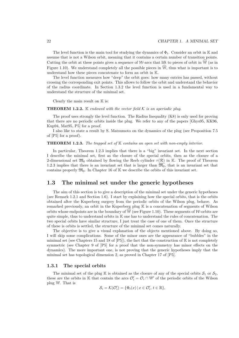
22 CHAPTER 1. A MINIMAL SET
The level function is the main tool for studying the dynamics of Φt. Consider an orbit in K andassume that is not a Wilson orbit, meaning that it contains a certain number of transition points.Cutting the orbit at these points gives a sequence of W-arcs that lift to pieces of orbit in W (as inFigure 1.10). We understand completely all the possible pieces in W, thus what is important is tounderstand how these pieces concatenate to form an orbit in K.
The level function measures how “deep” the orbit goes: how many entries has passed, withoutcrossing the corresponding exit points. This allows to follow the orbit and understand the behaviorof the radius coordinate. In Section 1.3.2 the level function is used in a fundamental way tounderstand the structure of the minimal set.
Clearly the main result on K is:
THEOREM 1.2.2. K endowed with the vector field K is an aperiodic plug.
The proof uses strongly the level function. The Radius Inequality (K8) is only used for provingthat there are no periodic orbits inside the plug. We refer to any of the papers [Ghys95, KK96,Kup94, Mat95, P5] for a proof.
I also like to state a result by S. Matsumoto on the dynamics of the plug (see Proposition 7.5of [P5] for a proof).
THEOREM 1.2.3. The trapped set of K contains an open set with non-empty interior.
In particular, Theorem 1.2.3 implies that there is a “big” invariant set. In the next sectionI describe the minimal set, first as the closure of the special orbits, then as the closure of a2-dimensional set M0 obtained by flowing the Reeb cylinder τ(R) in K. The proof of Theorem1.2.3 implies that there is an invariant set that is larger than M0, that is an invariant set thatcontains properly M0. In Chapter 16 of K we describe the orbits of this invariant set.
1.3 The minimal set under the generic hypothesesThe aim of this section is to give a description of the minimal set under the generic hypotheses
(see Remark 1.2.1 and Section 1.6). I start by explaining how the special orbits, that is the orbitsobtained after the Kuperberg surgery from the periodic orbits of the Wilson plug, behave. Asremarked previously, an orbit in the Kuperberg plug K is a concatenation of segments of Wilsonorbits whose endpoints are in the boundary of W (see Figure 1.10). These segments ofW-orbits arequite simple, thus to understand orbits in K one has to understand the rules of concatenation. Thetwo special orbits have similar structure, I just treat the case of one of them. Once the structureof these is orbits is settled, the structure of the minimal set comes naturally.
The objective is to give a visual explanation of the objects mentioned above. By doing so,I will skip some complications. Some of the minor ones are the appearance of “bubbles” in theminimal set (see Chapters 15 and 18 of [P5]), the fact that the construction of K is not completelysymmetric (see Chapter 9 of [P5] for a proof that the non-symmetry has minor effects on thedynamics). The more important one, is not proving that the generic hypotheses imply that theminimal set has topological dimension 2, as proved in Chapter 17 of [P5].
1.3.1 The special orbitsThe minimal set of the plug K is obtained as the closure of any of the special orbits S1 or S2,
these are the orbits in K that contain the arcs O′i = Oi ∩W′ of the periodic orbits of the Wilsonplug W. That is
Si = K(O′i) = Φt(x) |x ∈ O′i, t ∈ R,

1.3. THE MINIMAL SET UNDER THE GENERIC HYPOTHESES 23
observe that the endpoints of O′i ate the special points p(i) and p(i) defined in (1.7), for i = 1and 2. What follows explains why the periodic orbits of Wilson are not longer periodic after thesurgery, but it is not a proof of the aperiodicity of the plug. The explanation implies also thatSi ⊂ S1 for i = 1, 2 and when carried out for S2 (I do not give the details) we get that S1 = S2is a minimal set. Proving that this set is the only minimal set in the plug is a harder task: itinvolves understanding the asymptotic behavior of every orbit that is entirely contained in K. InProposition 7.1 of [P5], it is proved that the ω-limit of every point in K whose orbit stays in Kcontains S1, while its α-limit contains S2. Thus Σ = S1 = S2 is the unique minimal set.
We recall first from Figure 1.3 of the Wilson plug that the cylinder r = 2 contains the two
Figure 1.11: The cylinder r = 2 in W′
periodic orbits Oi for i = 1, 2. Consider the cylinder r = 2 in W′ containing the segments of orbitO′i for i = 1, 2. Since this cylinder intersects both insertions, in Figure 1.11 I erased two regions ofthe rectangle, one intersecting O1 and the other O2, corresponding to each insertion. Observe thatthese two regions are basically rectangles, with two of their sides tangent to the vector field andtwo transverse to the vector field. The transverse sides are either in the entrance of the insertionsL−i or in the exit of the insertions L+
i , for i = 1, 2.The orbit segment O′1 intersects the bottom entrance L−1 and the bottom exit L+
1 . Condition(K7) implies that the intersection with L−1 is at the special point p(1) that is identified with thepoint p′(1) = (2, θ1,−2) ∈ L−1 ∩ r = 2. That is σ1(p′(1)) = p(1), τ(p(1)) = τ(p′(1)) andr(p′(1)) = 2. By abuse of notation, let p(1) be the corresponding point in E1 ⊂ K. Likewise, theintersection of O′1 with L+
1 is at the special point p(1) that is identified with the point p′(1) =(2, θ1, 2) ∈ L+
1 ∩ r = 2. That is σ1(p′(1)) = p(1), τ(p(1)) = τ(p′(1)) and r(p′(1)) = 2. By abuseof notation, let p(1) be the corresponding point in S1 ⊂ K.
In general, I will use the same notation for points in L±i and their images under τ in Ei and Sifor i = 1, 2. The corresponding points in L±i are marked with a prime.
The positive K-orbit of a point in τ(O′1) continues after crossing E1 at p(1) as a trappedW-orbitin the cylinder r = 2, that is theW-orbit of p′(1). Since theW-orbit of p′(1) accumulates on O1,it intersects infinitely many times L−1 . Then the image under τ of this orbit intersects E1 = τ(L−1 )infinitely many times. Let p(1; 1, 1) be the first intersection. Denote by p′(1; 1, 1) ∈ L−1 the pointsuch that τ(p′(1; 1, 1)) = p(1; 1, 1), then the Radius Inequality (K8) implies that r(p′(1; 1, 1)) > 2.
We need the following important result (we refer to Propositions 6.5 and 6.7 of [P5]):
24 CHAPTER 1. A MINIMAL SET
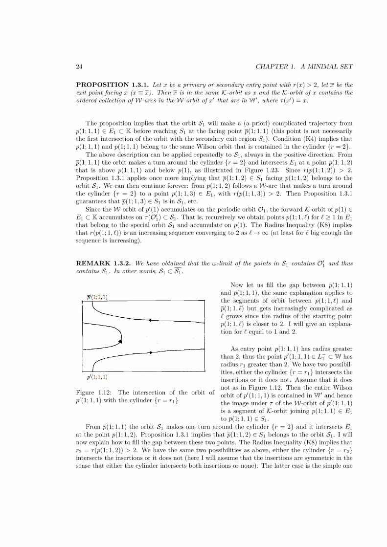
PROPOSITION 1.3.1. Let x be a primary or secondary entry point with r(x) > 2, let x be theexit point facing x (x ≡ x). Then x is in the same K-orbit as x and the K-orbit of x contains theordered collection of W-arcs in the W-orbit of x′ that are in W′, where τ(x′) = x.
The proposition implies that the orbit S1 will make a (a priori) complicated trajectory fromp(1; 1, 1) ∈ E1 ⊂ K before reaching S1 at the facing point p(1; 1, 1) (this point is not necessarilythe first intersection of the orbit with the secondary exit region S1). Condition (K4) implies thatp(1; 1, 1) and p(1; 1, 1) belong to the same Wilson orbit that is contained in the cylinder r = 2.
The above description can be applied repeatedly to S1, always in the positive direction. Fromp(1; 1, 1) the orbit makes a turn around the cylinder r = 2 and intersects E1 at a point p(1; 1, 2)that is above p(1; 1, 1) and below p(1), as illustrated in Figure 1.23. Since r(p(1; 1, 2)) > 2,Proposition 1.3.1 applies once more implying that p(1; 1, 2) ∈ S1 facing p(1; 1, 2) belongs to theorbit S1. We can then continue forever: from p(1; 1, 2) follows a W-arc that makes a turn aroundthe cylinder r = 2 to a point p(1; 1, 3) ∈ E1, with r(p(1; 1, 3)) > 2. Then Proposition 1.3.1guarantees that p(1; 1, 3) ∈ S1 is in S1, etc.
Since the W-orbit of p′(1) accumulates on the periodic orbit O1, the forward K-orbit of p(1) ∈E1 ⊂ K accumulates on τ(O′1) ⊂ S1. That is, recursively we obtain points p(1; 1, `) for ` ≥ 1 in E1that belong to the special orbit S1 and accumulate on p(1). The Radius Inequality (K8) impliesthat r(p(1; 1, `)) is an increasing sequence converging to 2 as `→∞ (at least for ` big enough thesequence is increasing).
REMARK 1.3.2. We have obtained that the ω-limit of the points in S1 contains O′1 and thuscontains S1. In other words, S1 ⊂ S1.
Figure 1.12: The intersection of the orbit ofp′(1; 1, 1) with the cylinder r = r1
Now let us fill the gap between p(1; 1, 1)and p(1; 1, 1), the same explanation applies tothe segments of orbit between p(1; 1, `) andp(1; 1, `) but gets increasingly complicated as` grows since the radius of the starting pointp(1; 1, `) is closer to 2. I will give an explana-tion for ` equal to 1 and 2.
As entry point p(1; 1, 1) has radius greaterthan 2, thus the point p′(1; 1, 1) ∈ L−1 ⊂W hasradius r1 greater than 2. We have two possibil-ities, either the cylinder r = r1 intersects theinsertions or it does not. Assume that it doesnot as in Figure 1.12. Then the entire Wilsonorbit of p′(1; 1, 1) is contained in W′ and hencethe image under τ of the W-orbit of p′(1; 1, 1)is a segment of K-orbit joining p(1; 1, 1) ∈ E1to p(1; 1, 1) ∈ S1.
From p(1; 1, 1) the orbit S1 makes one turn around the cylinder r = 2 and it intersects E1at the point p(1; 1, 2). Proposition 1.3.1 implies that p(1; 1, 2) ∈ S1 belongs to the orbit S1. I willnow explain how to fill the gap between these two points. The Radius Inequality (K8) implies thatr2 = r(p(1; 1, 2)) > 2. We have the same two possibilities as above, either the cylinder r = r2intersects the insertions or it does not (here I will assume that the insertions are symmetric in thesense that either the cylinder intersects both insertions or none). The latter case is the simple one

1.3. THE MINIMAL SET UNDER THE GENERIC HYPOTHESES 25
Figure 1.13: The intersection of the orbit of p′(1; 1, 2) with the cylinder r = r2
as treated for p(1; 1, 1). Now assume that the cylinder r = r2 intersects both insertions and alsothat the W-orbit of p′(1; 1, 2) intersects both insertions, as in Figure 1.13.
The intersection of theW-orbit of p′(1; 1, 2) with W′ is a collection ofW-arcs between transitionpoints, contained in the cylinder r = r2. The second part of Proposition 1.3.1 means that theimage under τ of all these arcs is contained in S1 and in the same order. Let us call these arcs Ajfor 1 ≤ j ≤ n for some finite n (n is finite since the W-orbit of p′(1; 1, 2) is finite, in Figure 1.13we have n = 5).
Clearly the image under τ of the arcs above does not completely fill the gap between p(1; 1, 2)and p(1; 1, 2), since it is not a connected set. To do so, we need to understand what happensbetween the endpoint of an arc Aj and the starting point of the following arc Aj+1.
Figure 1.14: The intersection of the orbit ofp′(1; 1, 2; 1, 1) with the cylinder r = r2,1
Let us follow the orbit from p(1; 1, 2) =τ(p′(1; 1, 2)). We start by the image under τ ofthe first arc A1. The assumptions imply thatthe endpoint of this arc is a point in E1 that wedenote by p(1; 1, 2; 1, 1). Let p′(1; 1, 2; 1, 1) ∈L−1 be the corresponding point. Observe thatthe Radius Inequality (K8) implies that r2 <r2,1 = r(p(1; 1, 2; 1, 1)). Again there are twopossibilities: either the cylinder r = r2,1 in-tersects the insertions or not. If not, the imageunder τ of theW-orbit p′(1; 1, 2; 1, 1) goes fromp(1; 1, 2; 1, 1) to the facing point p(1; 1, 2; 1, 1) ∈S1 joining A1 to A2. If yes we have to iteratethe description. Since each time that the orbitintersects a secondary entry point the radiusgrows, eventually it gets to a cylinder that does
not intersects any of the insertions. So assume, to make the discussion shorter, that we are in thesecond case, as in Figure 1.14.
Recapitulating, under the assumptions made, we have
p(1; 1, 1) τ(W−orbit)−−−−−−−→ p(1; 1, 1) W−arc−−−−→ p(1; 1, 2) τ(A1)−−−−→ p(1; 1, 2; 1, 1) τ(W−orbit)−−−−−−−→ p(1; 1, 2; 1, 1),

26 CHAPTER 1. A MINIMAL SET
where p(1; 1, 2; 1, 1) ∈ S1 is the starting point of the arc τ(A2) and it is facing p(1; 1, 2; 1, 1) bycondition (K4).
Now τ(A2) has its starting point in S1 and its endpoint either in E1 or in E2 (in Figure 1.12the endpoint of A2 is in L−1 with τ(L−1 ) = E1). Repeating the above description we fill in theorbit segment between the endpoint of τ(A2) and the starting point of τ(A3). We can thus jointhe collection of arcs τ(Aj) and find the K-orbit segment from p(1; 1, 1) to p(1; 1, 1).
The above description applies without any significant changes to the backward orbit of O′1.Indeed the backward orbit of a point in O′1 intersects L+
1 in the special point p(1) facing p(1) asin Figure 1.11. This point is identified with p′(1) ∈ L+
1 that has radius 2 and the intersectionof the backward W-orbit of this point with W′ is mapped under τ to parts of S1. Since this W-orbit accumulates in backward time on O2, then τ(O′2) is contained in the α-limit of S1 and thusS2 ⊂ S1. Also, recursively, in the backward direction, we can fill the gaps to describe the entireorbit.
This is a first explanation of how the orbit S1 is composed. In the rest of this section, alwaysadd “the image under τ” to the sets considered. I will explain basically the same construction ofS1, but in a new set of diagrams. For this we consider the level sets of S1. We need the followingresult (see Proposition 10.1 in [P5]).
PROPOSITION 1.3.3. For i = 1, 2, there is a well-defined level function
n0 : S1 ∪ S2 → N = 0, 1, 2, . . ., (1.9)
such that n−10 (0) = τ(O′1 ∪ O′2).
Figure 1.15: Level 0 and 1 of S1 with gaps
The level zero of n0|S1 is the arc τ(O′1) withendpoints p(1) and p(1), represented by thehorizontal segments in Figure 1.15. The levelone is composed by (the image under τ of) twosemi-infinite W-orbits: the forward W-orbit ofp′(1) and the backwardW-orbit of p′(1), repre-sented by the two vertical lines in Figure 1.15.Observe that the vertical lines are not contin-uous: the dotted parts correspond to the arcsthat are not in the intersection of these twoW-orbits with W′. In other words, in the left handside vertical line the continuous segments cor-respond (from top to bottom) to the arcs fromp(1) to p(1; 1, 1), from p(1; 1, 1) to p(1; 1, 2),from p(1; 1, 2) to p(1; 1, 3) and in general fromp(1; 1, `) to p(1; 1, ` + 1) for ` ≥ 1 and un-bounded. The right hand side vertical line isthe backward orbit of p(1) that repeatedly in-tersects the second insertion.
Let me point out one aspect in this newset of flattened diagrams. In the plug K theleft hand side vertical continuous segments inFigure 1.15 correspond to arcs that accumulate
on the horizontal segment τ(O′1), while the right hand side vertical continuous segments accumulateon τ(O′2).

1.3. THE MINIMAL SET UNDER THE GENERIC HYPOTHESES 27
The level 2 of S1 is composed by all the finite W-orbits starting at the intersections of the twolevel 1 orbits with E1 and E2. Thus by (the image under τ of) a countable collection of finiteW-orbits. Observe that since these are finite Wilson orbits, we just need to consider the starting
Figure 1.16: Level 0, 1 and 2 of S1 with gaps
point in the entrance of the insertions E1 ∪ E2, Proposition 1.3.1 implies that they will containthe facing points in the exit of the insertions S1 ∪ S2. I represent in Figure 1.16 these orbits asthe border of horizontal tongues, because of their shape inside W (as in Figures 1.2 and 1.3).Again the dotted parts are the segments that are not in the intersection with W′ and thus do notbelong to S1. As we travel downwards along the two level one W-orbits the tongues that appearat level 2 get longer, since the radius of their starting point gets closer to 2 and thus eventuallythey intersect the insertions. In Figure 1.16 (and Figure 1.17 below), the assumption is that theW-orbit of p′(1; 1, 1) does not intersects the insertions and theW-orbit of p′(1; 1, 2) does intersectsthe insertions. Then the intersection of the W-orbit of p′(1; 1, 2) with W′ is composed of the arcsAj for 1 ≤ j ≤ k and k finite. In Figure 1.16 the value of k is 3.
At any level n greater than 2, we consider the W-orbits of the points in the intersection of theW-orbits at level n− 1 with the entry regions E1 and E2. Recursively we obtain the diagram, inFigure 1.17, representing levels 0 to 4. This situation repeats again at any level, adding to thecomplexity of the diagram in Figure 1.17.
Observe that this set of diagrams explain the concatenation of pieces of Wilson orbits that formthe special orbit S1, but do not reflect how the orbit is embedded in K. The embedding is quitecomplicated by the nature of the maps σi, for i = 1, 2. In particular, the width of the tonguesthat appear is roughly the same and equals the width of the Reeb cylinder, as a consequence ofthe shape of Wilson orbits. I will come back to this point in Section 1.3.2.
In Figure 1.17, I marked a set of points: every finite W-orbit intersects the annulus z = 0at a single point. Condition (W1) implies that at this point the vector field W is vertical and bycondition (K3) this point is in W′ (since all the finite Wilson orbits we are considering have radiusgreater than 2). For a finite W-orbit we will call this point its tip.
Consider thus the set of tips contained in S1 and their lifts to W′. We obtain a countable setof points in the annulus z = 0, whose radii are arbitrarily close to 2. Hence the closed set S1

28 CHAPTER 1. A MINIMAL SET
Figure 1.17: The tree diagram for S1 with marked tips
contains points in τ(R′) the image of the Reeb cylinder in K.
We finish this section pointing out some conclusions:— Si ⊂ Sj for all i, j = 1, 2, thus S1 = S2 = Σ is the minimal set.— Σ contains points in τ(R′).
We are faced with a dichotomy: either the tips in S1 ∪S2 accumulate on a Cantor set in the circlez = 0, r = 2 contained in τ(R′) or they accumulate on the whole circle. Theorem 17.1 in [P5]states that under the generic hypotheses (see Remark 1.2.1 and Section 1.6), the tips accumulateon the whole circle, implying that Σ has topological dimension 2. A description of this set, moreprecisely a dense dimension 2 subset of Σ is given in the following section. We do not know if thereis a smooth Kuperberg plug for which the minimal set has dimension 1. In the piecewise linearcategory, G. Kuperberg and K. Kuperberg [KK96] construct a plug with a 1-dimensional minimalset.
1.3.2 M0, a dense subset of the minimal setIn this section I describe a dense dimension 2 subset of Σ for a generic Kuperberg flow, that
is denoted by M0. The set M0 is obtained by flowing inside K the notched Reeb cylinder τ(R′)and the description is very similar to the decomposition of S1 by levels explained in Figures 1.15,1.16 and 1.17. Before starting, I need to introduce two types of surfaces in W: finite and infinitepropellers.
For a moment, we will work in the Wilson plug. Consider a curve γ in the entry region ∂−h Wof the plug. We parametrize it as γ(t) with t ∈ [0, 1] and we assume that:
— r(γ(0)) = 3;— r(γ(1)) < r(γ(t)) for t ∈ [0, 1);— r(γ(1)) ≥ 2.
The propeller Pγ is obtained by flowing γ inside the Wilson plug. In the following figures weassume that γ is transverse to the cylinders r = cst., just to make the figures simpler.

1.3. THE MINIMAL SET UNDER THE GENERIC HYPOTHESES 29
Figure 1.18: Finite propeller inside W
If r(γ(1)) > 2 this is a simple game. Indeedthe W-orbit of every point in γ is finite, as itexits the plug in some finite time. The finitepropeller Pγ is the compact surface composedby the finite orbits of the points γ(t) for t ∈[0, 1]. It has the shape of a tongue that turnsin the positive θ-direction as in Figure 1.18.Its boundary is composed by γ in the entryregion of the plug, the facing curve γ in theexit region of the plug, the orbit of γ(0) that isjust a vertical segment in the vertical boundaryof the plug and the orbit of γ(1). Observe thatthe orbit of γ(1) gets longer as the radius ofγ(1) tends to 2.
If r(γ(1)) = 2 it is not so simple since theforward orbit of γ(1) is trapped. We considerin this case the forward orbits of the points in
the curve γ and the backward orbits of the points in the facing curve γ, for all times for which theorbits are defined. Equivalently, we consider the union of finite propellers Pγs for s ∈ [0, 1) andγs ⊂ γ the curve obtained as γ([0, s]) and the two semi-infinite orbits: the forward orbit of γ(1)and the backward orbit of the facing point γ(1). The infinite propeller Pγ is an open surface thatturns infinitely many times around the Reeb cylinder. Observe that we do not consider its closurethat consists of the union of Pγ and the Reeb cylinder R.
Figure 1.19: R′ ⊂W
Propellers are the blocks to build the sur-face M0 in the Kuperberg plug. To describeM0 we divide it by levels, Proposition 10.1 from[P5] states:
PROPOSITION 1.3.4. There is a well-defined level function
n0 : M0 → N = 0, 1, 2, . . ., (1.10)
such that n−10 (0) = τ(R′).
Let Mk0 ⊂M0 be the set of points at level at
must k, I describe next these sets for k = 0, 1, 2.
The level zero set is the image under τ ofthe notched Reeb cylinder R′ = R∩W′. In W′it is easy to visualize it (as in Figure 1.19), in Kit is a little bit more difficult. Figure 1.20 is anattempt to represent this set as it is embedded
in K ⊂ R3. What the map σ1 does to this cylinder is to choose a vertical segment in the cylinder(θ = θ1 in condition (K7)), turns it to make it tangent to part of the boundary of the cylinderthat got erased by the lower notch. Analogously, σ2 chooses a vertical segment in the cylinder(θ = θ2 in condition (K7)), turns it to make it tangent to part of the boundary of the cylinderthat got erased by the upper notch. The directions of the flow force the two turns to be in oppositedirections.
Observe that R′ ∩ L−1 is a vertical line that we call the curve γ (as in Figure 1.19) and letγ′ be the corresponding curve in L−1 (as in Figure 1.21). That is σ1(γ′) = γ and τ(γ′) = τ(γ).Analogously we have a curve λ ∈ L−2 and λ′ ∈ L−2 .
30 CHAPTER 1. A MINIMAL SET
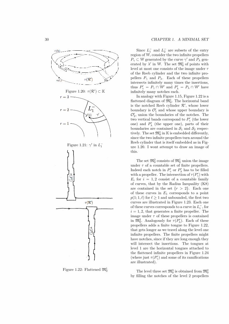
Figure 1.20: τ(R′) ⊂ K
Figure 1.21: γ′ in L−1
Figure 1.22: Flattened M10
Since L−1 and L−2 are subsets of the entryregion of W, consider the two infinite propellersPγ ⊂W generated by the curve γ′ and Pλ gen-erated by λ′ in W. The set M1
0 of points withlevel at most one consists of the image under τof the Reeb cylinder and the two infinite pro-pellers Pγ and Pλ. Each of these propellersintersects infinitely many times the insertions,thus P ′γ = Pγ ∩W′ and P ′λ = Pλ ∩W′ haveinfinitely many notches each.
In analogy with Figure 1.15, Figure 1.22 is aflattened diagram of M1
0. The horizontal bandis the notched Reeb cylinder R′, whose lowerboundary is O′1 and whose upper boundary isO′2, union the boundaries of the notches. Thetwo vertical bands correspond to P ′γ (the lowerone) and P ′λ (the upper one), parts of theirboundaries are contained in S1 and S2 respec-tively. The set M1
0 in K is embedded differently,since the two infinite propellers turn around theReeb cylinder that is itself embedded as in Fig-ure 1.20. I wont attempt to draw an image ofthis.
The set M20 consists of M1
0 union the imageunder τ of a countable set of finite propellers.Indeed each notch in P ′γ or P ′λ has to be filledwith a propeller. The intersection of τ(P ′γ) withEi for i = 1, 2 consist of a countable familyof curves, that by the Radius Inequality (K8)are contained in the set r > 2. Each oneof these curves in E1 corresponds to a pointp(1; 1, `) for ` ≥ 1 and unbounded, the first twocurves are illustrated in Figure 1.23. Each oneof these curves corresponds to a curve in L−i , fori = 1, 2, that generates a finite propeller. Theimage under τ of these propellers is containedin M2
0. Analogously for τ(P ′λ). Each of thesepropellers adds a finite tongue to Figure 1.22,that gets longer as we travel along the level oneinfinite propellers. The finite propellers mighthave notches, since if they are long enough theywill intersect the insertions. The tongues atlevel 1 are the horizontal tongues attached tothe flattened infinite propellers in Figure 1.24(where just τ(P ′γ) and some of its ramificationsare illustrated).
The level three set M30 is obtained from M2
0by filling the notches of the level 2 propellers

1.4. PSEUDOGROUPS 31
with finite propellers. Analogously Mk0 is obtained from Mk−1
0 by filling the notches of the levelk − 1 propellers with finite propellers. This process continues and gives the surface M0.
Under the generic hypotheses, the closure of M0 is the minimal set Σ. This means that the“boundary” of M0 that consists of the orbits S1 and S2 is dense in its interior. In Chapter 18 of[P5] we prove that Σ = M0 is a zippered lamination, roughly meaning that the interior has thestructure of a lamination (transversely Cantor) and the boundary is dense in the interior of theleaves. The definitions of interior and boundary for Σ are made precise in [P5]. I summarize thedescription in the last two sections with the following statement.
Figure 1.23: Curves in τ(P ′γ) ∩ E1
THEOREM 1.3.5 (Theorems 17.1 and 19.1 of [P5]). For a generic Kuperberg flow M0 = Σ isthe minimal set of the plug. The set Σ has topological dimension 2 and is stratified:
— it has an open 2-dimensional subset that forms a lamination with open leaves;— it has an open 1-dimensional subset that is dense in the previous set.
REMARK 1.3.6. Observe from Figure 1.24 that M0 has the structure of a tree whose branchescorrespond to the propellers and can be rooted by the choice of a point in τ(R′). The growth of thistree is then the growth of the leaves in the lamination of Theorem 1.3.5 and is studied in Chapter14 of [P5]. The growth is closely related to the growth of words in the pseudo?group G∗K , introducedin the next section.
1.4 PseudogroupsA novel tool introduced in [P5] that is used to study the dynamics of the flow, are the pseu-
dogroups and pseudo?group acting on an almost transverse rectangle. In a pseudo?group weconsider only compositions of a (symmetric) generating set, but we do not ask for the conditionon union of maps to be in the pseudo?group, as for pseudogroups. This section corresponds toparts of Chapter 9 of [P5], where all details and proofs can be consulted. I introduce here the mainmaps, that arise in the discussions in Sections 1.4.2 and 1.5 related to entropy.
In the plugs W and K we can consider the rectangles θ = cst., one of them in K is depictedin Figure 1.25.

32 CHAPTER 1. A MINIMAL SET
Figure 1.24: Flattened M0
Figure 1.25: A rectangle R0 in the Kuperberg Plug K

1.4. PSEUDOGROUPS 33
We must be careful to chose a value θ0 so that the rectangle R0 = θ = θ0 ⊂ W does notintersect either Di nor Di for i = 1 and 2. Let R0 be the corresponding rectangle in K, we use thesame notation since τ is bijective when restricted to such a rectangle. I will ask one more thingto this rectangle, that it lies between the two insertions as in Figure 1.25, so that from the upperpart (z > 0) points flow to the upper insertion and from the bottom part (z < 0) points flow tothe lower insertion.
Observe that, either in W or in K, the vector field is tangent to the rectangle near the boundaryand also at the line z = 0. Let ωi ∈ R0 be the intersection of the periodic orbit Oi with R0when considering the rectangle in W or the intersection of the arc O′i with R0 when consideringthe rectangle in K, for i = 1, 2.
A finite W-orbit, that is an orbit going from the entrance to the exit of the plug W, if itintersects R0, it does so in a symmetric pattern with respect to the line z = 0. In this case, theconstruction of the flow implies that the intersection consists of a finite sequence of points containedin the vertical line of constant radius (the value of the radius is determined by the orbit). We haveto consider two situations, either the orbit is tangent to R0 at the line z = 0 or not, in bothsituations the points in the intersection of the orbit with R0 are paired: for each point (r,−z) inthe intersection, (r, z) is also in the intersection (for z 6= 0).
We can define a first return map Ψ for the flow Ψt, that will have discontinuities (I refer toChapter 9 of [P5] for a complete discussion of the discontinuities and other properties of this map).The domain of Ψ is the set:
Dom(Ψ) ≡ ξ ∈ R0 | ∃ t > 0 such that Ψt(ξ) ∈ R0 and Ψs(ξ) /∈ R0 for 0 < s < t . (1.11)
The radius function is constant along the orbits of the Wilson flow, so that r(Ψ(ξ)) = r(ξ) for allξ ∈ Dom(Ψ). Also, note that the points ωi for i = 1, 2 are fixed-points for Ψ and for all otherpoints ξ ∈ R0 with ξ 6= ωi, points climb up that is z(Ψ(ξ)) > z(ξ).
Here I will consider just two types of first return maps for the flow Φt, instead of considering thegeneral first return map that is too complicated for a succinct discussion. For i = 1, 2, let Uφ+
i⊂ R0
be the subset consisting of points ξ such that the K-arc [ξ, η]K contains a single transition pointx ∈ Ei and its intersection with R0 is only at the endpoints ξ and η. Note that for such ξ, we seefrom Figures 1.10 and 1.25, that its K-orbit exits the surface Ei as theW-orbit of a point x′ ∈ L−iwith τ(x′) = x, flowing upwards from ∂−h W until it intersects R0 again. If the K-orbit of ξ entersEi but exits through Si before crossing R0, then it is not considered to be in the set Uφ+
i, since its
orbits contains more than one transition point before returning to R0. Let φ+i : Uφ+
i→ Vφ+
i. As
the K-arcs [ξ, η]K defining φ+i do not intersect A, the restricted map φ+
i is continuous. The setsUφ+
iand Vφ+
iare sketched in the left hand side illustration in Figure 1.26.
For i = 1, 2, let Uφ−i⊂ R0 be the subset of R0 consisting of points ξ such that the K-arc [ξ, η]K
contains a single transition point x ∈ Si and its intersection with R0 is only at the endpoints ξ andη. Then let φ−i : Uφ−
i→ Vφ−
i. Again, as the K-arcs [ξ, η]K defining the maps φ−i do not intersect
A, the restricted map φ−i is continuous. The sets Uφ−i
and Vφ−i
are sketched in the right hand sideillustration in Figure 1.26.
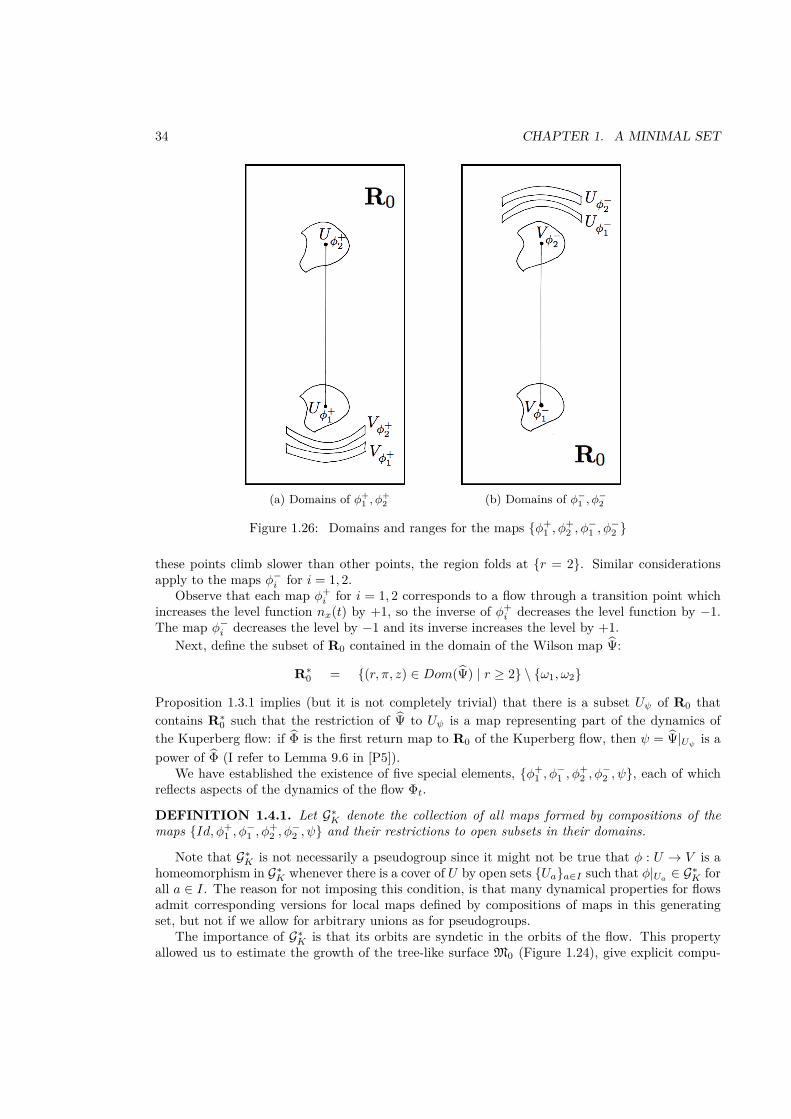
We comment on some details of the regions in Figures 1.26 (a) and (b). For the map φ+i ,
i = 1, 2, the domain contains a neighborhood of the point ωi. Flowing the domain Uφ+i
forward toEi and then applying the map σ−1
i we obtain a set Uφ+i⊂ L−i containing points with r-coordinate
equal to 2. Observe that the Radius Inequality implies that the maximum radius of points in Uφ+i
is bigger than the maximum radius of points in Uφ+i
. The first intersection of the W-orbits ofpoints in Uφ+
iwith R0 is thus a region containing points with r-coordinate equal to 2 and since
34 CHAPTER 1. A MINIMAL SET
(a) Domains of φ+1 , φ
+2 (b) Domains of φ−
1 , φ−2
Figure 1.26: Domains and ranges for the maps φ+1 , φ
+2 , φ
−1 , φ
−2
these points climb slower than other points, the region folds at r = 2. Similar considerationsapply to the maps φ−i for i = 1, 2.
Observe that each map φ+i for i = 1, 2 corresponds to a flow through a transition point which
increases the level function nx(t) by +1, so the inverse of φ+i decreases the level function by −1.
The map φ−i decreases the level by −1 and its inverse increases the level by +1.Next, define the subset of R0 contained in the domain of the Wilson map Ψ:
R∗0 = (r, π, z) ∈ Dom(Ψ) | r ≥ 2 \ ω1, ω2
Proposition 1.3.1 implies (but it is not completely trivial) that there is a subset Uψ of R0 thatcontains R∗0 such that the restriction of Ψ to Uψ is a map representing part of the dynamics ofthe Kuperberg flow: if Φ is the first return map to R0 of the Kuperberg flow, then ψ = Ψ|Uψ is apower of Φ (I refer to Lemma 9.6 in [P5]).
We have established the existence of five special elements, φ+1 , φ
−1 , φ
+2 , φ
−2 , ψ, each of which
reflects aspects of the dynamics of the flow Φt.
DEFINITION 1.4.1. Let G∗K denote the collection of all maps formed by compositions of themaps Id, φ+
1 , φ−1 , φ
+2 , φ
−2 , ψ and their restrictions to open subsets in their domains.
Note that G∗K is not necessarily a pseudogroup since it might not be true that φ : U → V is ahomeomorphism in G∗K whenever there is a cover of U by open sets Uaa∈I such that φ|Ua ∈ G∗K forall a ∈ I. The reason for not imposing this condition, is that many dynamical properties for flowsadmit corresponding versions for local maps defined by compositions of maps in this generatingset, but not if we allow for arbitrary unions as for pseudogroups.
The importance of G∗K is that its orbits are syndetic in the orbits of the flow. This propertyallowed us to estimate the growth of the tree-like surface M0 (Figure 1.24), give explicit compu-

1.4. PSEUDOGROUPS 35
tations for the entropy of the flow and the laminated entropy of M = M0 (I refer to Chapters 14,20, 21 and 22 of [P5]).
1.4.1 Shape of the minimal setIn this section, I present results in [P5] regarding topological properties of the minimal set Σ
for a generic Kuperberg flow. The space Σ is compact and connected, so is a continuum. Thenatural framework for the study of topological properties of spaces such as Σ is using shape theory.For example, Krystyna Kuperberg posed the question whether Σ has stable shape? Stable shapeis defined below and is about the nicest property one can expect for an exceptional minimal set.Theorem 1.4.5 below shows that Σ does not have stable shape. The proof of this result followsfrom the equality Σ = M0 for a generic flow and the structure theory developed in Section 1.3.2.It is a constructive proof: we describe in Chapter 23 of [P5] a system of generators for the firsthomology groups of a shape approximation (an example of such a generator is in Figure 1.27).
Shape theory studies the topological properties of a topological space Z using a form of Cechhomology theory. The definition of shape for a space Z embedded in the Hilbert cube was in-troduced by Borsuk [Bor68, Bor75]. We give a brief definition of the shape of a compactum Zembedded in a metric space X, following the work of Mardesic and Segal [MS82].
DEFINITION 1.4.2. A sequence U = U` | ` = 1, 2, . . . is called a shape approximation ofZ ⊂ X if:
1. each U` is an open neighborhood of Z in X which is homotopy equivalent to a compactpolyhedron;
2. U`+1 ⊂ U` for ` ≥ 1 and their closures satisfy⋂`≥1
U ` = Z.
Suppose that X,X ′ are connected manifolds, that U is a shape approximation for the compactsubset Z ⊂ X and U′ is a shape approximation for the compact subset Z′ ⊂ X ′. The compactaZ,Z′ are said to have the same shape if the following conditions are satisfied:
1. There is an order-preserving map φ : Z → Z and for each n ≥ 1 a continuous mapfn : Uφ(n) → U ′n such that for any pair n ≤ m, the restriction fn|Uφ(m) is homotopic tofm as maps from Uφ(m) to U ′n.
2. There is an order-preserving map ψ : Z → Z and for each n ≥ 1 a continuous mapgn : U ′ψ(n) → Un such that for any pair n ≤ m, the restriction gn|U ′ψ(m) is homotopicto gm as maps from U ′ψ(m) to Un.
3. For each n ≥ 1, there exists m ≥ maxn, φ ψ(n) such that the restriction of gn fψ(n) toUm is homotopic to the inclusion as maps from Um to Un.
4. For each n ≥ 1, there exists m ≥ maxn, ψ φ(n) such that the restriction of fn gφ(n) toU ′m is homotopic to the inclusion as maps from U ′m to U ′n.
DEFINITION 1.4.3. Let Z ⊂ X be a compact subset of a connected manifold X. Then theshape of Z is defined to be the equivalence class of a shape approximation of Z as above.
It is a basic fact of shape theory that this definition does not depend upon the choice of shapeapproximations and that two homotopic compacta have the same shape.

36 CHAPTER 1. A MINIMAL SET
Figure 1.27: A pseudo-orbit as generator of the homology of the shape approximation
DEFINITION 1.4.4. A compactum Z has stable shape if it is shape equivalent to a finitepolyhedron. That is, there exists a shape approximation U such that each inclusion ι : U`+1 → U`induces a homotopy equivalence and U1 has the homotopy type of a finite polyhedron.
Some examples of spaces with stable shape are compact manifolds and more generally finiteCW -complexes. A less obvious example is the minimal set for a Denjoy flow on T2 whose shapeis equivalent to the wedge of two circles. In particular, the minimal sets of the aperiodic C1-flow constructed by Schweitzer have stable shape, [Sch74]. The main result concerning genericKuperberg flows is the following.
THEOREM 1.4.5. The minimal set Σ of a generic Kuperberg flow does not have stable shape.
Another important definition in shape theory is the following.
DEFINITION 1.4.6. A compactum Z ⊂ X is said to be movable in X if for every neighborhoodU of Z, there exists a neighborhood U0 ⊂ U of Z such that, for every neighborhood W ⊂ U0 of Z,there is a continuous map ϕ : U0× [0, 1]→ U satisfying the condition ϕ(x, 0) = x and ϕ(x, 1) ∈Wfor every point x ∈ U0.
The notion of a movable compactum was introduced by Borsuk [Bor69], as a generalization ofspaces having the shape of an absolute neighborhood retract (ANR’s) and is an invariant of theshape of Z. It is a standard result that a compactum Z with stable shape is movable. The movableproperty distinguishes between the shape of a Hawaiian earring and a Vietoris solenoid; the formeris movable and the latter is not.
Showing the movable property for a space requires the construction of a homotopy retract ϕwith the properties stated in the definition, whose existence can be difficult to achieve in practice.There is an alternate condition on homology groups, weaker than the movable condition, which ismuch easier to check.
PROPOSITION 1.4.7. Let Z be a movable compacta with shape approximation U. Then thehomology groups satisfy the Mittag-Leffler Condition: For all ` ≥ 1, there exists p ≥ ` such thatfor any q ≥ p, the maps on homology groups for m ≥ 1 induced by the inclusion maps satisfy
Image Hm(Up;Z)→ Hm(U`;Z) = Image Hm(Uq;Z)→ Hm(U`;Z) . (1.12)
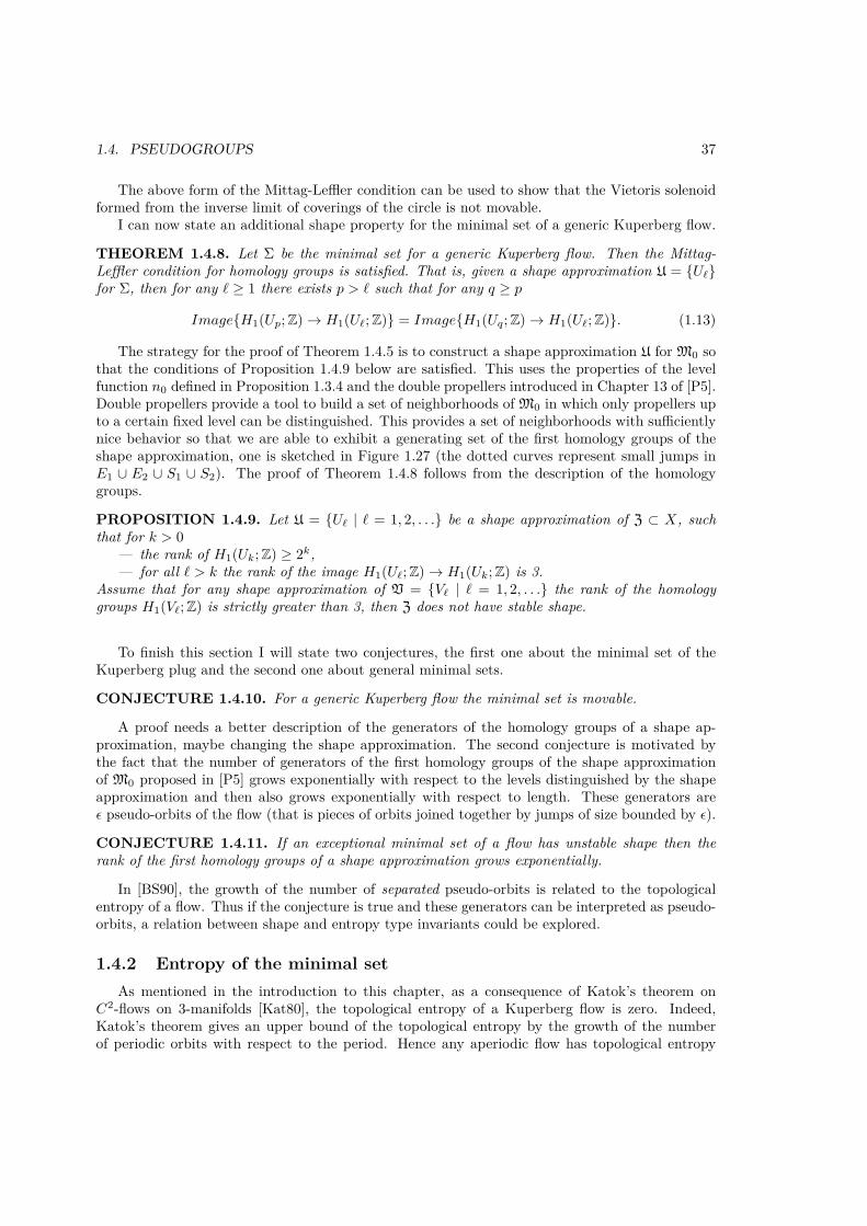
1.4. PSEUDOGROUPS 37
The above form of the Mittag-Leffler condition can be used to show that the Vietoris solenoidformed from the inverse limit of coverings of the circle is not movable.
I can now state an additional shape property for the minimal set of a generic Kuperberg flow.
THEOREM 1.4.8. Let Σ be the minimal set for a generic Kuperberg flow. Then the Mittag-Leffler condition for homology groups is satisfied. That is, given a shape approximation U = U`for Σ, then for any ` ≥ 1 there exists p > ` such that for any q ≥ p
ImageH1(Up;Z)→ H1(U`;Z) = ImageH1(Uq;Z)→ H1(U`;Z). (1.13)
The strategy for the proof of Theorem 1.4.5 is to construct a shape approximation U for M0 sothat the conditions of Proposition 1.4.9 below are satisfied. This uses the properties of the levelfunction n0 defined in Proposition 1.3.4 and the double propellers introduced in Chapter 13 of [P5].Double propellers provide a tool to build a set of neighborhoods of M0 in which only propellers upto a certain fixed level can be distinguished. This provides a set of neighborhoods with sufficientlynice behavior so that we are able to exhibit a generating set of the first homology groups of theshape approximation, one is sketched in Figure 1.27 (the dotted curves represent small jumps inE1 ∪ E2 ∪ S1 ∪ S2). The proof of Theorem 1.4.8 follows from the description of the homologygroups.
PROPOSITION 1.4.9. Let U = U` | ` = 1, 2, . . . be a shape approximation of Z ⊂ X, suchthat for k > 0
— the rank of H1(Uk;Z) ≥ 2k,— for all ` > k the rank of the image H1(U`;Z)→ H1(Uk;Z) is 3.
Assume that for any shape approximation of V = V` | ` = 1, 2, . . . the rank of the homologygroups H1(V`;Z) is strictly greater than 3, then Z does not have stable shape.
To finish this section I will state two conjectures, the first one about the minimal set of theKuperberg plug and the second one about general minimal sets.
CONJECTURE 1.4.10. For a generic Kuperberg flow the minimal set is movable.
A proof needs a better description of the generators of the homology groups of a shape ap-proximation, maybe changing the shape approximation. The second conjecture is motivated bythe fact that the number of generators of the first homology groups of the shape approximationof M0 proposed in [P5] grows exponentially with respect to the levels distinguished by the shapeapproximation and then also grows exponentially with respect to length. These generators areε pseudo-orbits of the flow (that is pieces of orbits joined together by jumps of size bounded by ε).
CONJECTURE 1.4.11. If an exceptional minimal set of a flow has unstable shape then therank of the first homology groups of a shape approximation grows exponentially.
In [BS90], the growth of the number of separated pseudo-orbits is related to the topologicalentropy of a flow. Thus if the conjecture is true and these generators can be interpreted as pseudo-orbits, a relation between shape and entropy type invariants could be explored.
1.4.2 Entropy of the minimal setAs mentioned in the introduction to this chapter, as a consequence of Katok’s theorem on
C2-flows on 3-manifolds [Kat80], the topological entropy of a Kuperberg flow is zero. Indeed,Katok’s theorem gives an upper bound of the topological entropy by the growth of the numberof periodic orbits with respect to the period. Hence any aperiodic flow has topological entropy
38 CHAPTER 1. A MINIMAL SET
zero. In [P5] we use G∗K , introduced in Definition 1.4.1, to make an explicit computation of thetopological entropy. This computation revealed chaotic behavior for the flow, but such that itevolves at a very slow rate and thus it does not result in positive topological entropy. We provedthat, under some extra hypotheses, such generic Kuperberg flows have positive slow entropy andthat the rates of chaotic behavior grow at a precise subexponential, but non-polynomial rate, asdiscussed in Chapter 21 of [P5].
To make the discussion more precise, let me give the definitions.Define the entropy of the flow Φt using a variation of the Bowen formulation of topological
entropy [Bow71] for a flow on a compact metric space (X, dX). The definition we adopt is symmetricin the role of the time variable t. Two points p, q ∈ X are said to be (ϕt, T, ε)-separated if
dX(ϕt(p), ϕt(q)) > ε for some − T ≤ t ≤ T .
A set E ⊂ X is (ϕt, T, ε)-separated if all pairs of distinct points in E are (ϕt, T, ε)-separated.Let s(ϕt, T, ε) be the maximal cardinality of a (ϕt, T, ε)-separated set in X. Then the topologicalentropy is defined by
htop(ϕt) = 12 · limε→0
lim supT→∞
1T
log(s(ϕt, T, ε)). (1.14)
Moreover, for a compact space X, the entropy htop(ϕt) is independent of the choice of metric dX .A relative form of the topological entropy for a flow ϕt can be defined for any subset Y ⊂ X,
by requiring that the collection of distinct (ϕt, T, ε)-separated points used in the definition (1.14)be contained in Y . The restricted topological entropy htop(ϕt|Y ) is bounded above by htop(ϕt).
I recall now the definition of entropy for pseudo?groups as introduced by Ghys, Langevin andWalzcak in [GLW88]. Let (X, dX) be a compact metric space and
G(1)X = ϕ0 = Id, ϕ1, ϕ
−11 , . . . , ϕk, ϕ
−1k
be a set of local homeomorphisms of X, with their inverses. Let GX denote the pseudogroupgenerated by the collection of maps G(1)
X . Let G∗X ⊂ GX denote the pseudo?group generated by thecompositions of maps in G(1)
X (as remarked after Definition 1.4.1, this might not be a pseudogroup).Let G(n)
X ⊂ G∗X be the collection of maps defined by the restrictions of compositions of at most nelements of G(1)
X .For ε > 0, say that x, y ∈ X are (G∗X , n, ε)-separated if there exists ϕ ∈ G(n)
X such that x, y arein the domain of ϕ and dX(ϕ(x), ϕ(y)) > ε. In particular, if the identity map is the only elementof G(n)
X which contains both x and y in its domain, then they are (G∗X , n, ε)-separated if and onlyif dX(x, y) > ε.
A finite set E ⊂ X is said to be (G∗X , n, ε)-separated if each distinct pair x, y ∈ E is (G∗X , n, ε)-separated. Let s(G∗X , n, ε) be the maximal cardinality of a (G∗X , n, ε)-separated subset of X.
Define the entropy of G∗X by:
hGLW (G∗X) = limε→0
lim supn→∞
1n
ln(s(G∗X , n, ε)). (1.15)
The property 0 < hGLW (G∗X) <∞ is independent of the choice of metric on X.
The third entropy type invariant I want to introduce is the slow entropy of a map, first defined inthe works of Katok and Thouvenot [KT97]. We adapted this idea for the action of a pseudo?group

1.5. VARIATIONS OF THE KUPERBERG PLUG 39
G∗X . For 0 < α < 1, define the α-entropy of G∗X , or just the slow entropy, by
hαGLW (G∗X) = limε→0
lim supn→∞
1nα
ln(s(G∗X , n, ε))
(1.16)
where 0 ≤ hαGLW (G∗X) ≤ ∞. If hαGLW (G∗X) > 0 and 0 < β < α, then hβGLW (G∗X) =∞. Analogously,one can define the slow entropy of a flow, by changing 1/T for 1/Tα in (1.14).
The strategy in [P5] is to relate the flow entropy to the entropy of the pseudo?group G∗K . Esti-mating the entropy of G∗K is equivalent to understanding how the tree M0 grows (see Remark 1.3.6).This is done by estimating the number of admissible words in the generators Id, φ+
1 , φ−1 , φ
+2 , φ
−2 , ψ
and their inverses (I refer to Chapter 14 in [P5]). We prove that, for a generic Kuperberg flow, thenumber of words is a subexponential function of the length and thus the entropy of G∗K is zero.
The computation suggests that there are exponentially many separated points, but the timethat the flow or the pseudo?group take to separate them is very long. We thus decided to studythe slow-entropy of the holonomy pseudo?group of the lamination that we denote by GM. I won’tgo into the details here, but this pseudo?group is generated by Id, φ+
1 , φ+2 , ψ and their inverses.
It turned out that to obtain that hαGLW (G∗M) > 0 for α = 1/2, we needed an extra hypothesis onthe radius function defined by the insertions, that we baptized as slow-growth. Theorem 21.10 of[P5] states
THEOREM 1.4.12. Let Φt be a generic Kuperberg flow. If the insertion maps σj have “slowgrowth”, then h
1/2GLW (G∗M) > 0.
That the slow entropy of the lamination is positive implies (via a computation similar to theone carried out in Chapter 20 of [P5]), that the slow entropy of the flow Φt is positive.
The words in the generators Id, φ+1 , φ
+2 , ψ used to prove Theorem 1.4.12 correspond to an
exponentially growing family of loops that appear as generators of the first homology groups inthe shape approximation used to prove Theorem 1.4.5. These two properties of Σ look very mucha like. I wonder if there is a general relation between the shape of a minimal set and the (slow)entropy of the flow.
CONJECTURE 1.4.13. Assume that a flow of a closed 3-manifold M has an exceptional min-imal set Σ whose shape is not stable, then the slow entropy of the flow is positive.
The assumption that the shape of Σ is not stable implies that the topological type of itsshape approximations keep changing as they become increasingly fine, while the assumption thatevery orbit of the flow in Σ is dense implies a type of recurrence for the topology of the shapeapproximations. The problem is then asking if these assumptions are sufficient to guarantee thatthe topological type of the approximations exhibit a form of self-similarity in their topological type,which implies that there are exponential separation of the points in the orbit of the flow, at somepossibly subexponential. This is closely related to Conjecture 1.4.11.
1.5 Positive entropy in a C∞-neighborhood of a genericKuperberg plug
As remarked above, the topological entropy of a Kuperberg is zero, but the computations in[P5] revealed some chaotic behavior. In [P7] we study a C∞-perturbation of a generic Kuperbergflow and we prove the following theorem.

40 CHAPTER 1. A MINIMAL SET
THEOREM 1.5.1. There exists a C∞ 1-parameter family of plugs Kε for ε ∈ (−1, a) for a > 0such that:
1. The plug K0 is a generic Kuperberg plug;2. For ε < 0, the flow in the plug Kε has two periodic orbits that bound an invariant cylinder,
every other orbit belongs to the wandering set and thus the flow has topological entropy zero;3. For ε > 0, the flow in Kε has positive topological entropy and an abundance of periodic
orbits.The proof of Theorem 1.5.1 for ε < 0 uses the same technical tools as developed in the previous
works [Kup94, KK96, Ghys95, Mat95] for the study of the dynamics of the Kuperberg plug K0. Theproof for ε > 0 uses in a fundamental way the technique of relating the dynamics of a Kuperberg-like flow to the dynamics of its return map to an almost transverse rectangle, by introducingsuitable pseudogroups as in Section 1.4.
I will not go into the details of the proof, but I explain the construction of the plugs Kε andgive the main ideas to understand their dynamics. These plugs are constructed exactly as K inSection 1.2.1 except that conditions (K7) and (K8) on the embeddings σεi (in place of σi) arereplaced by the following parametrized radius inequality. The embeddings σεi satisfy conditions(K1) to (K6) and are also required to satisfy two further conditions:
(K7ε) For i = 1, 2, the disk Li contains a point (2, θi) such that the image under σεi of thevertical segment (2, θi) × [−2, 2] ⊂ Di ⊂ W is contained in r = 2 + ε ∩ θ−i ≤ θ ≤ θ+
i ,and for ε = 0 it is contained in r = 2 ∩ θ−i ≤ θ ≤ θ
+i ∩ z = (−1)i.
(K8ε) Parametrized Radius Inequality: For all x′ = (r′, θ′,−2) ∈ L−i , let (r, θ, z) = σεi (r′, θ′,−2) ∈Lε−i , then r < r′ + ε unless x′ = (2, θi,−2) and then r = 2 + ε.
Observe that for ε = 0, we recover the Radius Inequality of Kuperberg, one of the mostfundamental concepts of Kuperberg’s construction. Figure 1.28 represents the radius inequalityfor ε < 0, ε = 0, and ε > 0. Note that in the third illustration (c) for the case ε > 0, the insertionhas a vertical shift upwards. This is not required by conditions (K7ε) and (K8ε), but it is used toprove the third part of Theorem 1.5.1.
(a) ε < 0 (b) ε = 0 (c) ε > 0
Figure 1.28: The modified radius inequality for the cases ε < 0, ε = 0 and ε > 0
The case ε < 0
In the case ε < 0, the self-insertions do not penetrate far enough as to trap the periodic orbits.Condition (K8ε) implies that the radius always grows at secondary entry points (without anyexceptions). For these plugs Proposition 1.3.1 is still valid. As a corollary we obtain that theKε-orbits containing the arcs Oεi = Oi ∩W′ε of the Wilson periodic orbits are periodic. Here
W′ε = W− (σε1(D1) ∪ σε2(D2)) ,

1.5. VARIATIONS OF THE KUPERBERG PLUG 41
in analogy with the definition of W′ (1.5). As stated in Theorem 1.5.1, these two orbits are theonly two periodic orbits of the flow in Kε. The proof of this last assertion is basically the same asthe proof of the aperiodicity of K = K0.
What I want to point out about this case is that it gives another way of understanding theminimal set of the original Kuperberg plug K = K0. In fact, the two periodic orbits of Kε forε < 0 bound an invariant cylinder Cε that is obtained by flowing inside Kε the notched Reebcylinder R′ε = R ∩W′ε. Indeed repeating the analysis in Section 1.3.2 we first point out thatProposition 1.3.4 is valid and we can consider as level 0 the set τε(R′ε) (where τε is defined as τ).This set intersects each entrance of an insertion along a curve contained in the region r > 2 andthus each curve generates a finite propeller that is at level 1 (see Figure 1.18 for an illustration ofa finite propeller in W).
As ε increases to zero, the length of these two level 1 propellers grows and when ε = 0 thepropellers become infinite. Hence for ε small enough, these two propellers at level 1 intersect theinsertions and thus give birth to propellers at level 2, etc. So we can build the cylinder Cε aswe built M0 in Section 1.3.2. The main difference is that for Cε the process stops: the level 1propellers are finite and thus intersect the insertions a finite number of times and this repeats atany level, and the maximum level attained in Cε is upper bounded by a number that depends onlyon ε. The set Cε is thus the union of the notched Reeb cylinder τε(R′ε) and a finite number offinite propellers.
A flattened illustration of Cε is basically the same as Figure 1.24, except that the two verticallevel one propellers τ(P ′γ) and τ(P ′λ) are finite propellers, implying that the process described byFigures 1.22 and 1.24 stops. The length of the two level 1 propellers increases as ε increases tozero, thus the complexity of the flattened diagram increases. We thus obtain an approximation ofM0 by embedded cylinders in R3.
The case ε > 0
The Radius Inequality in this case is illustrated in Figure 1.28 (c). Along the vertical liner = 2 the r′-coordinate is bounded below by 2 − ε, while the vertical line r = 3 does notintersects the insertion. This implies that there are values (between 2 + ε and 3), let me call oneof them a, of the radius such that along the vertical line r = a the r′-coordinate is boundedbelow by a. In [P7] we assume (for simplicity) that there is a unique such value, denoted by rε(see Lemma 1.6.5 and Hypothesis 1.6.6 in the following section for a precise statement). Thusfor points with r > rε, we have that the radius coordinate grows at secondary entry points. Thisimplies that Proposition 1.3.1 is valid when the hypothesis r > 2 is replaced by r > rε.
We can thus repeat the construction of the maps φ+1 , φ+
2 , φ−1 and φ−2 in Section 1.4 andunderstand their action on points with radius coordinate bigger than rε.
In order to prove Theorem 1.5.1 for ε > 0 we consider words in the generators Id, φ+1 , Ψ and
their inverses, for Ψ as in (1.11). The proof then follows in two steps:1. find a set V0 ⊂ R0 (for R0 as in Section 1.4) for which there exists `(ε) ∈ N such that for
every k ≥ `(ε) and ϕk = Ψk φ+1 we have that
— Uk = ϕk(V0) ∩ V0 6= ∅;— ϕk(Uk) ∩ Uk has two connected components.
2. proving that the invariant set of the maps ϕk, for each k ≥ `(ε), is an invariant set of theflow and that the return times to these set are bounded.
The first point guarantees the existence of a countable number of horseshoe like dynamics in thepseudo?group generated by Id, φ+
1 , Ψ. The second one says that these horseshoes are embeddedin the flow and the fact that the return times are bounded, allows to conclude that the topologicalentropy of the flow is positive. The vertical shift in Figure 1.28 is used to prove this second point.
42 CHAPTER 1. A MINIMAL SET
We do not understand how these horseshoes change as ε → 0 and disappear in the plug K0.One thing I understand is that the return times to the invariant sets grow as ε decreases, but theaspect that is not clear is what happens with all the periodic orbits in the plugs Kε for ε > 0. Isit just that their lengths blow up?
The bifurcation that is made explicit in Theorem 1.5.1 is highly not generic, but it might besurrounded by some type of generic bifurcations in the space of non-singular vector fields. Can wesay something about nearby bifurcations?
1.6 Generic hypothesesThe construction of aperiodic Kuperberg flows involve multiple choices, which do not change
whether the resulting flows are aperiodic, but do impact other dynamical properties of these flows.In this section, I present the assumptions made in the works [P5, P7], that are grouped under theword generic in the previous sections. In [P10] we discuss properties of the flow that depend on thegeneric hypotheses and discuss possible situations that can arise if these assumptions are dropped.This section thus gives a quick list of the hypotheses that were briefly explained in Remark 1.2.1.We discuss first the case for the traditional Kuperberg flows and afterward discuss the variationsof the construction to obtain the family Kε as in Section 1.5.
Recall that the modified Wilson vector field on W is given in (1.2) by
W = g(r, θ, z) ∂∂z
+ f(r, θ, z) ∂∂θ
where the function g(r, θ, z) = g(r, z) is the function g : R → [0, g0] which is non-negative, vanishingonly at the points (2,±1) and symmetric about the line z = 0. The function f(r, θ, z) = f(r, z)is assumed to satisfy the conditions (W1) to (W5).
Figure 1.3 illustrates the dynamics of the flow of W restricted to the cylinders r = cst. inW, for various values of the radius. It is clear from these pictures that the interesting part of thedynamics of this flow occurs on the cylinders with radius near to 2 and near the periodic orbits Oifor i = 1, 2.
The points (2,±1) ∈ R are the local minimum or maximum for the function g and thus itsmatrix of first derivatives must also vanish at these points and the Hessian matrix of secondderivatives must be positive semi-definite. The generic property for such a function is that theHessian matrix for g at these points is positive definite. In the works [P5, P7], a more preciseversion of this was formulated:
HYPOTHESIS 1.6.1. The function g satisfies the following conditions:
g(r, z) = g0 for (r − 2)2 + (|z| − 1)2 ≥ ε20 (1.17)
where 0 < ε0 < 1/4 is sufficiently small. Moreover, we require that the Hessian matrices of secondpartial derivatives for g at the vanishing points (2,±1) are positive definite. In addition, we requirethat g(r, z) is monotone increasing as a function of the distance
√(r − 2)2 + (|z| − 1)2 from the
points (2,±1).
Many of the results in [P5, P7] require this generic hypotheses for their proofs, as it allowsmaking estimates on the speed of ascent for the orbits of the Wilson flow near the periodic orbits.
The choices for the embeddings σi : Di → W, for i = 1, 2, as illustrated on Figures 1.7 and1.8, are more wide-ranging and have a fundamental influence on the dynamics of the resulting

1.6. GENERIC HYPOTHESES 43
Kuperberg flows on the quotient space K. We first impose a “normal form” condition on the inser-tions, which does not have significant impact on the dynamics, but allows a more straightforwardformulation of the other properties of the insertion maps.
Let (r, θ, z) = σi(x′) ∈ Di for i = 1, 2, where x′ = (r′, θ′, z′) ∈ Di is a point in the domain ofσi. Let πz(r, θ, z) = (r, θ,−2) denote the projection of W along the z-coordinate. We assume thatσi restricted to the bottom face, σi : L−i → W, has image transverse to the vertical fibers of πz.This normal form can be achieved by an isotopy of a given embedding along the flow lines of thevector field W, so does not change the orbit structure of the resulting vector field on the plug K.
The above transversality assumption implies that πz σi : L−i → W is a diffeomorphism intothe face ∂−h W, with image denoted by Di ⊂ ∂−h W. Then let ϑi = (πz σi)−1 : Di → L−i denotethe inverse map, so we have:
ϑi(r, θ,−2) = (r(ϑi(r, θ,−2)), θ(ϑi(r, θ,−2)),−2) = (Ri,r(θ),Θi,r(θ),−2) . (1.18)
We can then formalize in terms of the maps ϑi the assumptions on the insertion maps σi.
HYPOTHESIS 1.6.2 (Strong Radius Inequality). For i = 1, 2, assume that:1. σi : L−i →W is transverse to the fibers of πz;2. r = r(σi(r′, θ′, z′)) < r′, except for (2, θi, z′) and then z(σi(2, θi, z′)) = (−1)i;3. Θi,r(θ) = θ(ϑi(r, θ,−2)) is an increasing function of θ for each fixed r;4. Ri,r(θ) = r(ϑi(r, θ,−2)) has non-vanishing derivative for r = 2, except for the case of θi
defined by ϑi(2, θi,−2) = (2, θi,−2);5. For r sufficiently close to 2, we require that the θ derivative of Ri,r(θ) vanish at a unique
point denoted by θ(i, r), with θ(i, 2) = θi.Consequently, each surface L−i is transverse to the coordinate vector fields ∂/∂θ and ∂/∂z on W.
The illustration of the image of the curves r′ = 2 and r′ = 3 on Figure 1.8 suggests thatthese curves have “parabolic shape”. We formulate this notion more precisely using the functionϑi(r, θ,−2) defined by (1.18) and introduce the more general hypotheses they may satisfy. Recallthat ε0 > 0 was introduced in Hypothesis 1.6.1.
HYPOTHESIS 1.6.3. For i = 1, 2, 2 ≤ r0 ≤ 2 + ε0 and θi − ε0 ≤ θ ≤ θi + ε0, assume that
d
dθΘi,r0(θ) > 0 ,
d2
dθ2Ri,r0(θ) > 0 ,d
dθRi,r0(θi) = 0 . (1.19)
where θi satisfies ϑi(2, θi,−2) = (2, θi,−2). Thus for 2 ≤ r0 ≤ 2 + ε0, the graph of Ri,r0(θ) isconvex upwards with vertex at θ = θi.
Hypothesis 1.6.3 implies that all of the level curves r′ = c, for 2 ≤ c ≤ 2 + ε0, have parabolicshape, as the illustration in Figure 1.8 suggests.
We can now define what is called a generic Kuperberg flow in the work [P5].
DEFINITION 1.6.4. A Kuperberg flow Φt is generic if the Wilson flow W used in the construc-tion of the vector field K satisfies Hypothesis 1.6.1 and the insertion maps σi for i = 1, 2 used inthe construction of K satisfies Hypotheses 1.6.2, and Hypotheses 1.6.3.
That is, the singularities for the vanishing of the vertical component g · ∂/∂z of the vector fieldW are of quadratic type and the insertion maps used to construct K yield quadratic radius functionsnear the special points.
44 CHAPTER 1. A MINIMAL SET
Recall that the insertion maps for the variations from a Kuperberg flow as introduced in Sec-tion 1.5 are denoted by σεi : Di →W, for i = 1, 2. It is assumed that these maps satisfy the modifiedconditions (K7ε) and (K8ε). The illustrations of the radius inequality in Figure 1.28 again suggestthat the images of the curves r′ = c are of “quadratic type”. For ε < 0 there is no need to makeany further assumptions in the construction in order to obtain Theorem 1.5.1. In contrast, forε > 0 we need the analog of the generic hypotheses in Definition 1.6.4 and the existence of theradius rε as discussed in Section 1.5 and below.
We again assume the insertion maps σεi : L−i →W are transverse to the fibers of the projectionmap πz : W → ∂−h W along the z-coordinate. Then we can define the inverse map ϑεi = (πz σεi )−1 : Di → L−i and express the inverse map in polar coordinates as:
ϑεi(r, θ,−2) = (r(ϑεi(r, θ,−2)), θ(ϑεi(r, θ,−2)),−2) = (Rεi,r(θ),Θεi,r(θ),−2) . (1.20)
Then the level curves r′ = c pictured in Figure 1.28 are given by the maps θ′ 7→ πz(σεi (c, θ′,−2)) ∈∂−h W.
We note a straightforward consequence of the Parametrized Radius Inequality (K8ε). Recallthat θi is the radian coordinate specified in (K8ε) such that for x′ = (2, θi,−2) ∈ L−i we haver(σεi (2, θi,−2)) = 2 + ε. I refer to Lemma 6.1 in [P7].
LEMMA 1.6.5. For ε > 0 there exists 2 + ε < rε < 3 such that r(σεi (rε, θi,−2)) = rε.
We then add an additional assumption on the insertion maps σεi for i = 1, 2 which specifies thequalitative behavior of the radius function for r ≥ rε.
HYPOTHESIS 1.6.6. If rε is the smallest 2 + ε < rε < 3 such that r(σεi (rε, θi,−2)) = rε.Assume that r(σεi (r, θi,−2)) < r for r > rε.
The conclusion of Hypothesis 1.6.6 is implied by the Radius Inequality for the case ε = 0, butdoes not follow from the condition (K8ε) when ε > 0.
We can now formulate the analog of Hypothesis 1.6.2, which imposes uniform conditions onthe derivatives of the maps ϑεi , for the plugs Kε with ε > 0. Recall that 0 < ε0 < 1/4 was specifiedin Hypothesis 1.6.1 and we assume that 0 < ε < ε0.
HYPOTHESIS 1.6.7 (Strong Radius Inequality). For i = 1, 2, assume that:1. σεi : L−i →W is transverse to the fibers of πz;2. r = r(σεi (r′, θ′, z)) < r + ε, except for x′ = (2, θi, z) and then r = 2 + ε;3. Θε
i,r(θ) is an increasing function of θ for each fixed r;4. For 2 − ε0 ≤ r ≤ 2 + ε0 and i = 1, 2, assume that Rεi,r(θ) has non-vanishing derivative,
except when θ = θi as defined by ϑεi(2 + ε, θi,−2) = (2, θi,−2);5. For r sufficiently close to 2 + ε, we require that the θ derivative of Rεi,r(θ) vanishes at a
unique point denoted by θ(i, r).
Note that Hypotheses 1.6.6 and 1.6.7 combined imply that rε is the unique value of 2+ε < rε < 3for which r(σεi (rε, θi,−2)) = rε. We can then formulate the analog of Hypothesis 1.6.3.
HYPOTHESIS 1.6.8. For 2− ε0 ≤ r0 ≤ 2 + ε0 and θi − ε0 ≤ θ ≤ θi + ε0, assume that
d
dθΘεi,r0
(θ) > 0 ,d2
dθ2Rεi,r0
(θ) > 0 ,d
dθRεi,r0
(θi) = 0 . (1.21)
where θi satisfies ϑεi(2, θi,−2) = (2, θi,−2). Thus for 2− ε0 ≤ r0 ≤ 2 + ε0, the graph of Rεi,r0(θ) is
convex upwards with vertex at θ = θi.
1.6. GENERIC HYPOTHESES 45
Finally, we have the definition of the generic Φεt flows of the plugs Kε, as introduced in Sec-tion 1.5 and studied in [P7].
DEFINITION 1.6.9. The flow Φεt is generic if the Wilson flow W used in the construction ofthe vector field Kε satisfies Hypothesis 1.6.1 and the insertion maps σεi for i = 1, 2 used in theconstruction of Kε satisfies Hypotheses 1.6.7, and Hypotheses 1.6.8.

46 CHAPTER 1. A MINIMAL SET

Chapter 2
Trunkenness, an asymptoticinvariant for flows
This chapter covers the results of my work with P. Dehornoy [P9]. The problem we addressis the construction of new invariants of volume-preserving vector fields on S3, or on compact do-mains of R3, up to volume-preserving diffeomorphisms. This problem is motivated by at leasttwo physical situations. First if v is the velocity field of a time-dependent ideal fluid satisfyingthe Euler equations (ideal hydrodynamics) then its vorticity field curl v is transported by the flowof v [Hel1858]. Second if B is the magnetic field of an incompressible plasma (ideal magnetody-namics), then B turns out to be transported by the velocity field as long as the latter does notdevelop singularities [Wol58]. In these contexts, invariants of curl v or B up to volume-preservingdiffeomorphisms yield time-independent invariants of the system.
Not so many such invariants exist. The first one was discovered by W. Thomson [Tho1867]: ifthe considered field has a periodic orbit or a periodic tube, then its knot type is an invariant (thisremark led to the development of knot theory by P. G. Tait [Tait1877]). However it may not beeasy to find periodic orbits and even then such an invariant only takes a small part of the fieldinto account.
The main known invariant is called helicity. It is defined by the formula Hel(v) =∫v ·u, where
u = curl−1(v) is an arbitrary vector-potential of v. It was discovered by Woltjer, Moreau andMoffatt [Wol58, Mor61, Mof69]. Helicity is easy to compute or to approximate since it is enough toexhibit a vector-potential of the considered vector field, to take the scalar product and to integrate.The connection with knot theory was sketched by Moffatt [Mof69] and deepened by Arnold [Arn73]as follows. Denote by kX(p, t) a loop starting at the point p, tangent to the vector field X for atime t and closed by an arbitrary segment of bounded length. Denote by Lk the linking number ofloops. Arnold showed that for almost every p1, p2, the limit lim
t1,t2→∞
1t1t2
Lk(kX(p1, t1), kX(p2, t2))exists (see also [Vog02] for a corrected proof). Moreover, if X is ergodic the limit coincides almosteverywhere with Hel(X) (for a non-ergodic vector field, one has to average the previous limit toobtain the helicity).
The idea of considering knot invariants of long pieces of orbits of the vector field was pursued byGambaudo and Ghys [GG01] who considered ω-signatures of knots, Baader [Baa11] who consideredlinear saddle invariants, and Baader and Marche [BM12] who considered Vassiliev’s finite typeinvariants. In every case, it is shown that limt→∞
1tnV (kX(p, t)) exists, where V is the considered
invariant and n a suitable exponent called the order of the asymptotic invariant. However all theseconstructions have the drawback that they do not yield any new invariant for ergodic vector fields,since the obtained limits are all functions of the helicity.
47

48 CHAPTER 2. TRUNKENNESS, AN ASYMPTOTIC INVARIANT FOR FLOWS
Recently, it was proved by Kudryavtseva for vector fields obtained by suspending an area-preserving diffeomorphism of a surface [Kud14] and for non-vanishing vector fields [Kud16] andthen by Enciso, Peralta-Salas and Torres de Lizaur [EPT16] for arbitrary volume-preserving vectorfields, that every invariant that is regular integral (in the sense that its Frechet derivative is theintegral of a continuous kernel) is a function of helicity. I will not state the precise statements.These results give a satisfactory explanation of why most constructions yield invariants that arefunctions of helicity for ergodic vector fields. However they do not rule out the existence of otherinvariants, but imply that such invariants cannot be too regular.
An example of such another invariant is the asymptotic crossing number considered by Freed-man and He [FH91]. The advantage is that it is not proportional to helicity, but the disadvantageis that it is hard to compute, even on simple examples.
In [P9] we consider a less well-known knot invariant called the trunk (see Definition 2.0.1 below).It was defined by Ozawa [Ozw10], building on the concept of thin position that was introduced byGabai [Gab87] for solving the R-conjecture. Less famous than the invariants previously studiedin the context of vector fields, the trunk has the advantage that its definition relies on surfacestransverse to the considered knot, so that it is easy to transcript in the context of vector fields.The invariant depends on an invariant measure for the flow of the vector field that may or maynot be a volume and is invariant under homeomorphisms that preserve this measure. Given aµ-preserving vector field X and a surface S, the geometric flux through S is the infinitesimalvolume that crosses S in both directions (see Definition 2.0.4), we denote it by Flux(X,µ, S). Ourinvariant is a minimax of the geometric flux, where one minimizes over all height functions andmaximizes over the levels of the considered height function.
To motivate our definition, I will start by defining the trunk of a knot. Let K be a knot,embedded in R3. The standard height function on R3 is the function hz : R3 → R, (x, y, z) 7→ z.Every level h−1
z (t) is a 2-dimensional plane. A height function on R3 is a function obtained byprecomposing hz by an orientation preserving diffeomorphism, that is, a function of the form
h : R3 → R(x, y, z) 7→ hz(φ(x, y, z))
for φ an orientation preserving diffeomorphism of R3. In particular, a height function is a functionwhose levels are smooth planes. A height function h is said to be in Morse position with respectto K if the restriction of h to K is a Morse function. In this case there are only finitely many pointsat which K is tangent to a level of h. We denote this set of functions by height Morse functions.
DEFINITION 2.0.1. Assume that K is an embedded knot in R3 that is in Morse position withrespect to hz. The trunk of the curve K relatively to hz is
tkhz (k) := maxt∈R
]K ∩ h−1z (t).
The trunk of a knot K is then defined by
Tk(K) := minh height
Morse function
tkh(K) = minh height
Morse function
maxt∈R
]K ∩ h−1(t).
One can define the trunk of knot by fixing the height function and changing the embedding ofthe knot K in R3, see [Zup12].
EXAMPLE 2.0.2. A knot is trivial if and only if its trunk equals 2. Indeed the embedding asthe boundary of a vertical disk shows that the trunk is less than or equal to 2 and every embedding
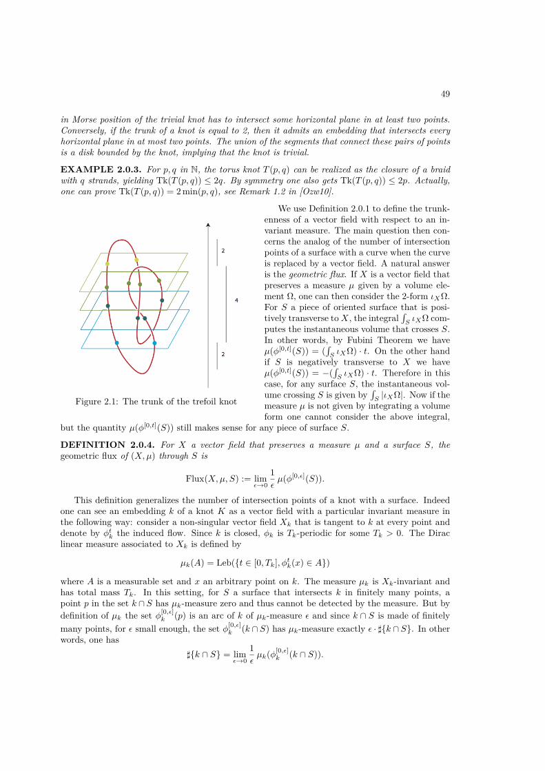
49
in Morse position of the trivial knot has to intersect some horizontal plane in at least two points.Conversely, if the trunk of a knot is equal to 2, then it admits an embedding that intersects everyhorizontal plane in at most two points. The union of the segments that connect these pairs of pointsis a disk bounded by the knot, implying that the knot is trivial.
EXAMPLE 2.0.3. For p, q in N, the torus knot T (p, q) can be realized as the closure of a braidwith q strands, yielding Tk(T (p, q)) ≤ 2q. By symmetry one also gets Tk(T (p, q)) ≤ 2p. Actually,one can prove Tk(T (p, q)) = 2 min(p, q), see Remark 1.2 in [Ozw10].
Figure 2.1: The trunk of the trefoil knot
We use Definition 2.0.1 to define the trunk-enness of a vector field with respect to an in-variant measure. The main question then con-cerns the analog of the number of intersectionpoints of a surface with a curve when the curveis replaced by a vector field. A natural answeris the geometric flux. If X is a vector field thatpreserves a measure µ given by a volume ele-ment Ω, one can then consider the 2-form ιXΩ.For S a piece of oriented surface that is posi-tively transverse toX, the integral
∫SιXΩ com-
putes the instantaneous volume that crosses S.In other words, by Fubini Theorem we haveµ(φ[0,t](S)) = (
∫SιXΩ) · t. On the other hand
if S is negatively transverse to X we haveµ(φ[0,t](S)) = −(
∫SιXΩ) · t. Therefore in this
case, for any surface S, the instantaneous vol-ume crossing S is given by
∫S|ιXΩ|. Now if the
measure µ is not given by integrating a volumeform one cannot consider the above integral,
but the quantity µ(φ[0,t](S)) still makes sense for any piece of surface S.
DEFINITION 2.0.4. For X a vector field that preserves a measure µ and a surface S, thegeometric flux of (X,µ) through S is
Flux(X,µ, S) := limε→0
1εµ(φ[0,ε](S)).
This definition generalizes the number of intersection points of a knot with a surface. Indeedone can see an embedding k of a knot K as a vector field with a particular invariant measure inthe following way: consider a non-singular vector field Xk that is tangent to k at every point anddenote by φtk the induced flow. Since k is closed, φk is Tk-periodic for some Tk > 0. The Diraclinear measure associated to Xk is defined by
µk(A) = Leb(t ∈ [0, Tk], φtk(x) ∈ A)
where A is a measurable set and x an arbitrary point on k. The measure µk is Xk-invariant andhas total mass Tk. In this setting, for S a surface that intersects k in finitely many points, apoint p in the set k ∩ S has µk-measure zero and thus cannot be detected by the measure. But bydefinition of µk the set φ[0,ε]
k (p) is an arc of k of µk-measure ε and since k ∩ S is made of finitelymany points, for ε small enough, the set φ[0,ε]
k (k ∩ S) has µk-measure exactly ε · ]k ∩ S. In otherwords, one has
]k ∩ S = limε→0
1εµk(φ[0,ε]
k (k ∩ S)).

50 CHAPTER 2. TRUNKENNESS, AN ASYMPTOTIC INVARIANT FOR FLOWS
As µk is concentrated on k, we thus have
]k ∩ S = limε→0
1εµk(φ[0,ε]
k (S)) = Flux(Xk, µk, S), (2.1)
so the geometric flux indeed generalizes the number of intersection points.We now mimic for vector fields the definition of the trunk of a knot. In order to have a well-
defined maximum, in what follows we assume the vector fields are on a compact domain D3 ⊂ R3
or on the 3-sphere S3 = R3 ∪∞. In the later case, we define the standard height function
h0 : S3 → [0, 1]
(x, y, z) 7→ 1− 11 + x2 + y2 + z2 .
The levels h−10 (0) and h−1
0 (1) consist of the points (0, 0, 0) and ∞ respectively and every otherlevel h−1
0 (t) is a 2-dimensional sphere centered at the origin. A height function on S3 is then afunction obtained by precomposing by an orientation preserving diffeomorphism φ of S3, that is,a function of the form h : S3 → [0, 1], (x, y, z) 7→ h0(φ(x, y, z)).DEFINITION 2.0.5. Let X be a vector field whose flow preserves a measure µ on a compactdomain of R3 or on S3 and h a height function. We set
tksh(X,µ) := maxt∈[0,1]
Flux(X,µ, h−1(t)) = maxt∈[0,1]
limε→0
1εµ(φ[0,ε](h−1(t))).
The trunkenness of (X,µ) is defined as
Tks(X,µ) := infh heightfunction
tksh(X,µ) = infh heightfunction
maxt∈[0,1]
Flux(X,µ, h−1(t))
= infh heightfunction
maxt∈[0,1]
limε→0
1εµ(φ[0,ε](h−1(t))).
Note that we can only consider an infimum instead of a minimum as in the case of knots. InTheorem 2.0.11 we study the implications of having a height function achieving the trunkenness.
If the invariant measure µ is given by the integration of a volume form Ω, we get the alternativedefinitions
tksh(X,Ω) = maxt∈[0,1]
∫h−1(t)
|ιXΩ|, and Tks(X,Ω) = infh heightfunction
maxt∈[0,1]
∫h−1(t)
|ιXΩ|.
From Definition 2.0.5 it is straightforward that the trunkenness of a vector field is invariantunder diffeomorphisms that preserve the measure µ. More is true, the trunkenness is invariantunder homeomorphisms that preserve µ.THEOREM 2.0.6. Assume that X1 and X2 are vector fields on S3 or on a compact domainof R3 that preserve a probability measure µ and that there is a µ-preserving homeomorphism f thatconjugates the flows of X1 and X2. Then we have
Tks(X1, µ) = Tks(X2, µ).
What we do in [P9] is to prove several properties of this new invariant. The first one is acontinuity result, that is more easily stated in terms of currents, but we also provide corollariesthat do not rely on this vocabulary. Given a vector field X and a measure µ, we can define anormal 1-current C(X,µ): for α any differential 1-form C(X,µ)(α) =
∫α(X)dµ, where the integral
is taken on the ambient space. We consider the space of normal currents endowed with the masstopology (see [Mor00]).

51
THEOREM 2.0.7. The trunkenness is a continuous functional on the space of normal currents.
COROLLARY 2.0.8. Suppose that (Xn, µn)n∈N is a sequence of measure-preserving vector fieldssuch that (Xn)n∈N converges to X in the C0-topology and (µn)n∈N converges to µ in the weak-∗sense. Then we have
limn→∞
Tks(Xn, µn) = Tks(X,µ).
Now for p a point in the ambient manifold and t > 0, denote by kX(p, t) the closed curveobtained by concatenating the orbit segment between p and φtX(p) and a short path between thesetwo points. As for the asymptotic linking number, there is a system of short paths such thatwe obtain a simple closed curve for µ-almost all points and almost all times [Vog02]. The nextcorollary states that the trunkenness is an asymptotic invariant in the sense of Arnold [AK98] andits order is 1.
COROLLARY 2.0.9. Assume that X is a µ-preserving vector field and that X is ergodic withrespect to µ, then for µ-almost every p the limit
limt→∞
1tTk(kX(p, t))
exists and is equal to Tks(X,µ).
Theorem 2.0.7 allows to compute the trunkenness of Seifert flows on S3, as explained in Sec-tion 2.1. These computations in turn show that the trunkenness is not dictated by helicity, evenin the case of ergodic vector fields, thus contrasting with most previously known knot-theoreticalconstructions.
THEOREM 2.0.10. There is no function f such that for every ergodic volume-preserving vectorfield X on S3 one has Tks(X,µ) = f(Hel(X,µ)).
Finally we address the question of what happens if for a non-singular vector field on S3 thereis a function that achieves the trunkenness, or in other words if the infimum in Definition 2.0.5 isa minimum.
THEOREM 2.0.11. Let X be a non-singular vector field on S3 preserving the measure µ and ha height function such that
Tks(X,µ) = maxt∈[0,1]
Flux(X,µ, h−1(t))
Then X has an unknotted periodic orbit.
One of the main motivations for constructing topological invariants of a vector field X is tofind lower bounds on the energies Ep(X) :=
∫|X|p dµ. Indeed since a topological invariant yields
a time-independent invariant of the physical system, an energy bound in terms of a topologicalinvariant will also be time-independent, although the energy may vary when the vector field istransported under (volume-preserving) diffeomorphisms. Such energy bounds exist for the helicityand for the asymptotic crossing number. We do not know whether the trunkenness bounds theenergy, a possible path towards finding an inequality between the trunk and the energy is to relatethe trunk to the crossing number that is itself related to helicity.

52 CHAPTER 2. TRUNKENNESS, AN ASYMPTOTIC INVARIANT FOR FLOWS
2.1 Independence of helicityAs mentioned in the introduction, the helicity is a well-known invariant of vector fields up
to volume-preserving diffeomorphism. In this section, all vector fields are on the sphere S3 andpreserve a volume form, that we denote by Ω. For X such a vector field, Cartan’s formula impliesthat ιXΩ is a closed 2-form and since the ambient manifold is simply connected it is exact. Wemay then write ιXΩ = dα, for α some differential 1-form. The helicity of X can be defined as
Hel(X) :=∫S3α ∧ dα,
and does not depends on the choice of the primitive α [AK98].As we recalled in the introduction, most known asymptotic invariants are in fact proportional to
the helicity [Arn73, GG01, Baa11, BM12]. The goal of this section it to prove that the trunkennessof a vector field is not a function of its helicity. In order to do so we compute the trunkenness andthe helicity of a vector field that preserves the invariant tori of a Hopf fibration of S3.
Considering S3 as the unit sphere (z1, z2) ∈ C2, |z1|2+|z2|2 = 1, the Seifert flow of slope (α, β)is the flow φα,β given by
φtα,β(z1, z2) := (z1ei2παt, z2e
i2πβt),
generated by the vector field Xα,β . This flow preserves the standard volume form, that is, thevolume form ΩHaar associated to the Haar measure of S3. The flow has two distinctive periodicorbits corresponding to z1 = 0 and z2 = 0 that are trivial knots in S3. The tori |z1/z2| = r for0 < r < ∞ are invariant and the flow on each one of them is the linear flow of slope α/β. If α/βis rational, put α/β = p/q with p, q ∈ N coprime. Then every orbit of φα,β , different from the twotrivial ones, is a torus knot of type T (p, q).
The helicity of φα,β is equal to αβ. To compute it in the rational case (α, β) = (p, q) withp, q coprime, observe that all the orbits except two are periodic of period 1. The linking numberof an arbitrary pair of such orbits is pq. Therefore the asymptotic linking number (also calledasymptotic Hopf invariant) equals pq and, by Arnold’s Theorem [Arn73], so does the helicity. Forthe general case of (α, β) not necessarily rational, it is enough to use the continuity of the helicity,since Xα,β can be approximated by a sequence of Seifert flows with rational slope.
PROPOSITION 2.1.1. The trunkenness of the Seifert flow φα,β with respect to the standardvolume form ΩHaar is equal to 2 min(α, β).
Proof. Let us first prove Tks(Xα,β ,ΩHaar) ≤ 2β. For this it is enough to exhibit a height function hthat yields tksh(Xα,β ,ΩHaar) = 2β. First define ∞ = (0, 1) and 0 = (0,−1) in S3 ⊂ C2 and takethe stereographic projection to identify
(z1, z2) ∈ C2 , |z1|2 + |z2|2 = 1 ' R3 ∪ ∞.
Take now as h the standard height function h0 of R3 ∪ ∞. The spheres are centered at 0 ∈ R3
that corresponds to the point (0,−1) ∈ S3 ⊂ C2, hence the orbit z1 = 0 intersects twice each levelsphere h−1
0 (t). The middle sphere, S = h−10 (1/2), contains the other special orbit z2 = 0 and is
the only sphere that intersects all the orbits of φα,β . Then the function t 7→∫h−1
0 (t) |ιXα,βΩHaar|has a maximum for t = 1/2.
For computing∫S|ιXα,βΩHaar|, we remark that the 2-sphere S has the orbit (ei2παt, 0) as an
equator, that the flow is positively transverse to the northern hemisphere and negatively trans-verse to the southern hemisphere. Then the integral
∫S|ιXα,βΩHaar| is equal to twice the flux
of Xα,β through any disk bounded by the curve (ei2παt, 0). Consider the flat disk D in S3
bounded by (ei2παt, 0). The first return time to D is constant and equal to 1/β, so the flux

2.1. INDEPENDENCE OF HELICITY 53
multiplied by 1/β gives the total volume of S3, that is 1. Therefore Flux(Xα,β ,ΩHaar, D) isequal to β and we obtain tksh0(Xα,β ,ΩHaar) =
∫S|ιXα,βΩHaar| = 2β. By symmetry, we then
have Tks(Xα,β ,ΩHaar) ≤ 2 min(α, β).
For proving the converse inequality Tks(Xα,β ,ΩHaar) ≥ 2 min(α, β), we approximate Xα,β (inthe C∞-topology) by a sequence (Xpn/rn,qn/rn)n∈N, where pn, qn, rn are integer numbers. Theo-rem 2.0.8 yields
Tks(Xα,β ,ΩHaar) = limn→∞
Tks(Xpn/rn,qn/rn ,ΩHaar).
As the trunkenness is an order-1 invariant (which means that it is multiplied by λ if the vectorfield is multiplied by λ), we only have to prove Tks(Xp,q,ΩHaar) = 2 min(p, q) for p, q two coprimenatural numbers.
Since every orbit of Xp,q is periodic, we can consider a sequence (Kn)n∈N of collections ofperiodic orbits whose induced normalized linear Dirac measures µn converge to ΩHaar. We takeKn to be an n-component link all of whose components are torus knots T (p, q). Actually Kn is acabling with n strands on T (p, q), so by Zupan’s theorem [Zup12], the trunk of Kn is 2nmin(p, q).Since the period of each component of Kn is 1, the total length of Kn is n and we get
Tks(Xp,q,ΩHaar) = limn→∞
Tks(Xp,q, µn) = limn→∞
2 min(p, q) = 2 min(p, q).
Proof of Theorem 2.0.10. The previous computations show that for a Seifert flow Xα,β on S3
we have Hel(Xα,β ,ΩHaar) = αβ and Tks(Xα,β ,ΩHaar) = 2 min(α, β). There is no real func-tion g such that min(α, β) = g(αβ), so there is no function g such that Tks(Xα,β ,ΩHaar) =g(Hel(Xα,β ,ΩHaar)).
However the Seifert flows are not ergodic with respect to ΩHaar. Indeed, the foliation of S3 byinvariant tori is invariant, so that it is easy to construct an invariant set with arbitrary measure.Still, a theorem of Katok [Kat73] states that the vector field Xα,β can be perturbed (in the C1-topology) into an ergodic one. Starting from X1,8 and X2,4 and applying Katok’s argument, weobtain two ergodic volume-preserving vector fields X ′1,8 and X ′2,4. By continuity, their trunknessesare close to 2 and 4 respectively, while their helicities are close to 8. At the expense of multiplyingthe X ′1,8 and X ′2,4 by a constant, we can assume that their helicities are exactly 8. However theirtrunknesses are still close to 2 and 4, hence different.
The formula Tks(Xα,β ,ΩHaar) = 2 min(α, β) is also interesting to compare with Kudryavtseva’sand Encisco-Peralata-Salas-Torres de Lizaur’s theorems: the function (α, β) 7→ 2 min(α, β) is con-tinuous but not differentiable, so that trunkenness is a continuous vector field invariant, but it isnot integral regular in the sense of [Kud16, EPT16].

54 CHAPTER 2. TRUNKENNESS, AN ASYMPTOTIC INVARIANT FOR FLOWS

Bibliography
[Arn73] V. I. Arnold, The asymptotic Hopf invariant and its applications, Proc. Summer Schoolin Diff. Equations at Dilizhan, 1973 (1974), Evevan (in Russian); English transl. Sel. Math.Sov., 5, 327–345, 1986.
[AK98] V. I. Arnold and B. Khesin, Topological methods in hydrodynamics, Appl. Math. Sci.,125, Springer, 1998.
[Baa11] S. Baader, Asymptotic concordance invariants for ergodic vector fields, Comment. Math.Helv., 86, 1–12, 2011.
[BM12] S. Baader and J. Marche, Asymptotic Vassiliev invariants for vector fields, Bull. Soc.Math. France, 140, 569–582, 2012.
[BS90] M. Barge and R. Swanson, Pseudo-orbits and topological entropy, Proc. of the A.M.S,109, 2, 559–566, 1990.
[Bor68] K. Borsuk, Concerning homotopy properties of compacta, Fund. Math., 62, 223–254,1968.
[Bor69] K. Borsuk, On movable compacta, Fund. Math., 66, 137–146, 1969.[Bor75] K. Borsuk, Theory of shape, Monografie Mat., vol. 59, Polish Science Publ., Warszawa,
1975.[Bow71] R. Bowen, Entropy for group endomorphisms and homogeneous spaces, Trans. Amer.
Math. Soc., 153, 401–414, 1971.[P9] P. Dehornoy and A. Rechtman, The trunkenness of a volume-preserving vector field, to
appear in Nonlinearity.[EPT16] A. Enciso, D. Peralta-Salas and F. Torres de Lizaur, Helicity is the only integral
invariant of volume-preserving transformations, Proc. Natl. Acad. Sci. USA, 113, 2035–2040,2016.
[FH91] M. H. Freedman and Z.-X. He, Divergence-Free Fields: Energy and Asymptotic CrossingNumber, Ann. of Math., 134, 189–229, 1991.
[Gab87] D. Gabai, Foliations and the topology of 3-manifolds III, J. Differential Geom., 26,479–536, 1987.
[GG01] J.-M. Gambaudo and E. Ghys, Signature asymptotique d’un champ de vecteurs en di-mension 3, Duke Math. J., 106, 41–79, 2001.
[Ghys95] E. Ghys, Construction de champs de vecteurs sans orbite periodique (d’apres KrystynaKuperberg), Seminaire Bourbaki, Vol. 1993/94, Exp. No. 785, Asterisque, 227, 283–307, 1995.
[GLW88] E. Ghys, R. Langevin and P. Walczak, Entropie geometrique des feuilletages, ActaMath., 160, 105–142, 1988.
[Han80] M. Handel, One-dimensional minimal sets and the Seifert conjecture, Ann. of Math.(2), 111, 35–66, 1980.
55
56 BIBLIOGRAPHY
[Har88] J.C. Harrison, C2 counterexamples to the Seifert conjecture, Topology, 27, 249–278,1988.
[Hel1858] H. von Helmholtz, Uber Integrale der hydrodynamischen Gleichungen, welche denWirbelbewegungen entsprechen, J. Reine Angew. Math., 55, 25–55, 1858.
[Hof93] H. Hofer, Pseudoholomorphic curves in symplectizations with applications to the Wein-stein conjecture in dimension three, Invent. Math., 114, 3, 515–563, 1993.
[HI] S. Hurder and D. Ingebretson, Smooth flows with fractional entropy dimension, in prepa-ration.
[P5] S. Hurder and A. Rechtman, The dynamics of generic Kuperberg flows, Asterisque, 377,1–250, 2016.
[P7] S. Hurder and A. Rechtman, Aperiodicity at the boundary of chaos, to appear at ErgodicTheory and Dynamical Systems.
[P10] S. Hurder and A. Rechtman, Perspectives on Kuperberg flows, to appear at the proceed-ings of the 31st Summer Conference on Topology and its Applications.
[Kat73] A. Katok, Ergodic perturbations of degenerate integrable Hamiltonian systems, Math.USSR Izv., 7, 535, 1973.
[Kat80] A. Katok, Lyapunov exponents, entropy and periodic orbits for diffeomorphisms, Inst.Hautes Etudes Sci. Publ. Math., 51, 137–173, 1980.
[KT97] A. Katok and J.-P. Thouvenot, Slow entropy type invariants and smooth realization ofcommuting measure-preserving transformations, Ann. Inst. H. Poincare Probab. Statist., 33,323–338, 1997.
[Kni81] R. J. Knill, A C∞ flow on S3 with a Denjoy minimal set, J. Differential Geom., 16, no.2, 271 – 280, 1981.
[Kud14] E. A. Kudryavtseva, Conjugation invariants on the group of area-preserving diffeomor-phisms of the disk, Math. Notes, 95, 877–880, 2014.
[Kud16] E. A. Kudryavtseva, Helicity is the only invariant of incompressible flows whose deriva-tive is continuous in C1-topology, Math. Notes, 99, 611–615, 2016.
[Kup96] G. Kuperberg, A volume-preserving counterexample to the Seifert conjecture, Com-ment. Math. Helv., 71, 70–97, 1996.
[Kup94] K. Kuperberg, A smooth counterexample to the Seifert conjecture, Ann. of Math. (2),140, 723–732, 1994.
[KK96] G. Kuperberg and K. Kuperberg, Generalized counterexamples to the Seifert conjec-ture, Ann. of Math. (2), 144, 239–268, 1996.
[MS82] S. Mardesic and J. Segal, Shape theory: The inverse system approach, North-HollandMath. Library, Vol. 26, North-Holland Publishing Co., Amsterdam, 1982.
[Mat95] S. Matsumoto, Kuperberg’s C∞ counterexample to the Seifert conjecture, Sugaku,Mathematical Society of Japan, 47, 38–45, 1995. Translation: Sugaku Expositions, 11,39–49, 1998, Amer. Math. Soc.
[Mof69] K. Moffatt The degree of knottedness of tangle vortex lines, J. Fluid. Mech., 106,117–129, 1969.
[Mor61] J.-J. Moreau, Constantes d’un ılot tourbillonnaire en fluide parfait barotrope, C. R.Acad. Sci. Paris, 252, 2810–2812, 1961.
[Mor00] F. Morgan, Geometric measure theory. A beginner’s guide, Third edition, AcademicPress, Inc., San Diego, CA, 2000.

BIBLIOGRAPHY 57
[Ozw10] M. Ozawa, Waist and trunk of knots, Geom. Dedicata, 149, 85âĂŞ94, 2010.[PW77] P.B. Percell and F.W. Wilson, Jr., Plugging flows, Trans. Amer. Math. Soc., 233,
93–103, 1977.[Sch74] P.A. Schweitzer, Counterexamples to the Seifert conjecture and opening closed leaves of
foliations, Ann. of Math. (2), 100, 386–400, 1974.[Tho73] E.S. Thomas, Jr. One-dimensional minimal sets, Topology, 12, 233–242, 1973.[Tait1877] P. Tait, On knots, Trans. Roy. Soc. Edin., 28, 145–190, 1877.[Tau09] C. H. Taubes, An observation concerning uniquely ergodic vector fields on 3-manifolds,
J. Gokova Geom. Topol. GGT 3, 9 –21, 2009.[Tho1867] W. Thomson, On Vortex Atoms, Proc. Roy. Soc. Edinburgh, 6, 94–105, 1867; reprinted
in Phil. Mag., 34, 15–24, 1867.[Vog02] T. Vogel, On the asymptotic linking number, Proc. Amer. Math. Soc., 131, 2289–2297,
2002.[Wil66] F.W. Wilson, Jr., On the minimal sets of non-singular vector fields, Ann. of Math. (2),
84, 529–536, 1966.[Wol58] L. Woltjer, A Theorem on Force-free magnetic Fields, Proc. Natl. Acad. Sci. USA, 44,
489–491, 1958.[Zup12] A. Zupan, A lower bound on the width of satellite knots, Topology Proc., 40, 179–188,
2012.


![Beyond Kuperberg Flows - homepages.math.uic.eduhomepages.math.uic.edu/~hurder/talks/Bedlewo20130603.pdf · Beyond Kuperberg Flows ... [Harrison, 1988] Replace the circular orbits](https://static.fdocuments.us/doc/165x107/5b1513da7f8b9ab6778d7e9d/beyond-kuperberg-flows-hurdertalksbedlewo20130603pdf-beyond-kuperberg-flows.jpg)