
Aspects of Twistor Geometry and Supersymmetric Field ...
280
Aspects of Twistor Geometry and Supersymmetric Field Theories within Superstring Theory Von der Fakult¨ at f¨ ur Mathematik und Physik der Universit¨ at Hannover zur Erlangung des Grades Doktor der Naturwissenschaften Dr. rer. nat. genehmigte Dissertation von ChristianS¨amann geboren am 23. April 1977 in Fulda
Transcript of Aspects of Twistor Geometry and Supersymmetric Field ...

Aspects of Twistor Geometry
and Supersymmetric Field Theories
within Superstring Theory
Von der Fakultat fur Mathematik und Physik der Universitat Hannover
zur Erlangung des Grades
Doktor der Naturwissenschaften
Dr. rer. nat.
genehmigte Dissertation von
Christian Samann
geboren am 23. April 1977 in Fulda


For there is nothing hidden, except that it should be made known;neither was anything made secret, but that it should come to light.
Mark 4,22
Wir mussen wissen, wir werden wissen.David Hilbert


To those who taught me

Betreuer: Prof. Dr. Olaf Lechtenfeld und Dr. Alexander D. PopovReferent: Prof. Dr. Olaf LechtenfeldKorreferent: Prof. Dr. Holger Frahm
Tag der Promotion: 30.01.2006
Schlagworte: Nichtantikommutative Feldtheorie, Twistorgeometrie, StringtheorieKeywords: Non-Anticommutative Field Theory, Twistor Geometry, String Theory
ITP-UH-26/05

Zusammenfassung
Die Resultate, die in dieser Arbeit vorgestellt werden, lassen sich im Wesentlichen zweiForschungsrichtungen in der Stringtheorie zuordnen: Nichtantikommutative Feldtheoriesowie Twistorstringtheorie.
Nichtantikommutative Deformationen von Superraumen entstehen auf naturliche Wei-se bei Typ II Superstringtheorie in einem nichttrivialen Graviphoton-Hintergrund, undsolchen Deformationen wurde in den letzten zwei Jahren viel Beachtung geschenkt. Zu-nachst konzentrieren wir uns auf die Definition der nichtantikommutativen Deformationvon N = 4 super Yang-Mills-Theorie. Da es fur die Wirkung dieser Theorie keine Super-raumformulierung gibt, weichen wir statt dessen auf die aquivalenten constraint equationsaus. Wahrend der Herleitung der deformierten Feldgleichungen schlagen wir ein nichtan-tikommutatives Analogon zu der Seiberg-Witten-Abbildung vor.
Eine nachteilige Eigenschaft nichantikommutativer Deformationen ist, dass sie Super-symmetrie teilweise brechen (in den einfachsten Fallen halbieren sie die Zahl der erhal-tenen Superladungen). Wir stellen in dieser Arbeit eine sog. Drinfeld-Twist-Technik vor,mit deren Hilfe man supersymmetrische Feldtheorien derart reformulieren kann, dass diegebrochenen Supersymmetrien wieder manifest werden, wenn auch in einem getwistetenSinn. Diese Reformulierung ermoglicht es, bestimmte chirale Ringe zu definieren undergibt supersymmetrische Ward-Takahashi-Identitaten, welche von gewohnlichen super-symmetrischen Feldtheorien bekannt sind. Wenn man Seibergs naturalness argument,welches die Symmetrien von Niederenergie-Wirkungen betrifft, auch im nichtantikom-mutativen Fall zustimmt, so erhalt man Nichtrenormierungstheoreme selbst fur nichtan-tikommutative Feldtheorien.
Im zweiten und umfassenderen Teil dieser Arbeit untersuchen wir detailliert geome-trische Aspekte von Supertwistorraumen, die gleichzeitig Calabi-Yau-Supermannigfal-tigkeiten sind und dadurch als target space fur topologische Stringtheorien geeignet sind.Zunachst stellen wir die Geometrie des bekanntesten Beispiels fur einen solchen Super-twistorraum, CP 3|4, vor und fuhren die Penrose-Ward-Transformation, die bestimmteholomorphe Vektorbundel uber dem Supertwistorraum mit Losungen zu den N = 4supersymmetrischen selbstdualen Yang-Mills-Gleichungen verbindet, explizit aus. An-schließend diskutieren wir mehrere dimensionale Reduktionen des SupertwistorraumesCP 3|4 und die implizierten Veranderungen an der Penrose-Ward-Transformation.
Fermionische dimensionale Reduktionen bringen uns dazu, exotische Supermannig-faltigkeiten, d.h. Supermannigfaltigkeiten mit zusatzlichen (bosonischen) nilpotenten Di-mensionen, zu studieren. Einige dieser Raume konnen als target space fur topologischeStrings dienen und zumindest bezuglich des Satzes von Yau fugen diese sich gut in dasBild der Calabi-Yau-Supermannigfaltigkeiten ein.
Bosonische dimensionale Reduktionen ergeben die Bogomolny-Gleichungen sowie Ma-trixmodelle, die in Zusammenhang mit den ADHM- und Nahm-Gleichungen stehen.(Tatsachlich betrachten wir die Supererweiterungen dieser Gleichungen.) Indem wir bes-timmte Terme zu der Wirkung dieser Matrixmodelle hinzufugen, konnen wir eine kom-plette Aquivalenz zu den ADHM- und Nahm-Gleichungen erreichen. Schließlich kanndie naturliche Interpretation dieser zwei Arten von BPS-Gleichungen als spezielle D-Branekonfigurationen in Typ IIB Superstringtheorie vollstandig auf die Seite der topo-logischen Stringtheorie ubertragen werden. Dies fuhrt zu einer Korrespondenz zwischentopologischen und physikalischen D-Branesystemen und eroffnet die interessante Perspek-tive, Resultate von beiden Seiten auf die jeweils andere ubertragen zu konnen.


Abstract
There are two major topics within string theory to which the results presented in thisthesis are related: non-anticommutative field theory on the one hand and twistor stringtheory on the other hand.
Non-anticommutative deformations of superspaces arise naturally in type II super-string theory in a non-trivial graviphoton background and they have received much at-tention over the last two years. First, we focus on the definition of a non-anticommutativedeformation of N = 4 super Yang-Mills theory. Since there is no superspace formulationof the action of this theory, we have to resort to a set of constraint equations defined onthe superspace R4|16
~ , which are equivalent to the N = 4 super Yang-Mills equations. Inderiving the deformed field equations, we propose a non-anticommutative analogue of theSeiberg-Witten map.
A mischievous property of non-anticommutative deformations is that they partiallybreak supersymmetry (in the simplest case, they halve the number of preserved super-charges). In this thesis, we present a so-called Drinfeld-twisting technique, which allowsfor a reformulation of supersymmetric field theories on non-anticommutative superspacesin such a way that the broken supersymmetries become manifest even though in somesense twisted. This reformulation enables us to define certain chiral rings and it yields su-persymmetric Ward-Takahashi-identities, well-known from ordinary supersymmetric fieldtheories. If one agrees with Seiberg’s naturalness arguments concerning symmetries oflow-energy effective actions also in the non-anticommutative situation, one even arrivesat non-renormalization theorems for non-anticommutative field theories.
In the second and major part of this thesis, we study in detail geometric aspectsof supertwistor spaces which are simultaneously Calabi-Yau supermanifolds and whichare thus suited as target spaces for topological string theories. We first present thegeometry of the most prominent example of such a supertwistor space, CP 3|4, and makeexplicit the Penrose-Ward transform which relates certain holomorphic vector bundlesover the supertwistor space to solutions to theN = 4 supersymmetric self-dual Yang-Millsequations. Subsequently, we discuss several dimensional reductions of the supertwistorspace CP 3|4 and the implied modifications to the Penrose-Ward transform.
Fermionic dimensional reductions lead us to study exotic supermanifolds, which aresupermanifolds with additional even (bosonic) nilpotent dimensions. Certain such spacescan be used as target spaces for topological strings, and at least with respect to Yau’stheorem, they fit nicely into the picture of Calabi-Yau supermanifolds.
Bosonic dimensional reductions yield the Bogomolny equations describing static mo-nopole configurations as well as matrix models related to the ADHM- and the Nahmequations. (In fact, we describe the superextensions of these equations.) By adding cer-tain terms to the action of these matrix models, we can render them completely equivalentto the ADHM and the Nahm equations. Eventually, the natural interpretation of thesetwo kinds of BPS equations by certain systems of D-branes within type IIB superstringtheory can completely be carried over to the topological string side via a Penrose-Wardtransform. This leads to a correspondence between topological and physical D-brane sys-tems and opens interesting perspectives for carrying over results from either sides to therespective other one.

Contents
Chapter I. Introduction 15I.1 High-energy physics and string theory . . . . . . . . . . . . . . . . . . 15I.2 Epistemological remarks . . . . . . . . . . . . . . . . . . . . . . . . . . 19I.3 Outline . . . . . . . . . . . . . . . . . . . . . . . . . . . . . . . . . . . 21I.4 Publications . . . . . . . . . . . . . . . . . . . . . . . . . . . . . . . . 23
Chapter II. Complex Geometry 25II.1 Complex manifolds . . . . . . . . . . . . . . . . . . . . . . . . . . . . . 25
II.1.1 Manifolds . . . . . . . . . . . . . . . . . . . . . . . . . . . . 25II.1.2 Complex structures . . . . . . . . . . . . . . . . . . . . . . 27II.1.3 Hermitian structures . . . . . . . . . . . . . . . . . . . . . 28
II.2 Vector bundles and sheaves . . . . . . . . . . . . . . . . . . . . . . . . 31II.2.1 Vector bundles . . . . . . . . . . . . . . . . . . . . . . . . . 31II.2.2 Sheaves and line bundles . . . . . . . . . . . . . . . . . . . 35II.2.3 Dolbeault and Cech cohomology . . . . . . . . . . . . . . . 36II.2.4 Integrable distributions and Cauchy-Riemann structures . 39
II.3 Calabi-Yau manifolds . . . . . . . . . . . . . . . . . . . . . . . . . . . 41II.3.1 Definition and Yau’s theorem . . . . . . . . . . . . . . . . . 41II.3.2 Calabi-Yau 3-folds . . . . . . . . . . . . . . . . . . . . . . . 43II.3.3 The conifold . . . . . . . . . . . . . . . . . . . . . . . . . . 44
II.4 Deformation theory . . . . . . . . . . . . . . . . . . . . . . . . . . . . 46II.4.1 Deformation of compact complex manifolds . . . . . . . . . 46II.4.2 Relative deformation theory . . . . . . . . . . . . . . . . . 47
Chapter III. Supergeometry 49III.1 Supersymmetry . . . . . . . . . . . . . . . . . . . . . . . . . . . . . . . 49
III.1.1 The supersymmetry algebra . . . . . . . . . . . . . . . . . 50III.1.2 Representations of the supersymmetry algebra . . . . . . . 51
III.2 Supermanifolds . . . . . . . . . . . . . . . . . . . . . . . . . . . . . . . 52III.2.1 Supergeneralities . . . . . . . . . . . . . . . . . . . . . . . . 53III.2.2 Graßmann variables . . . . . . . . . . . . . . . . . . . . . . 54III.2.3 Superspaces . . . . . . . . . . . . . . . . . . . . . . . . . . 56III.2.4 Supermanifolds . . . . . . . . . . . . . . . . . . . . . . . . 58III.2.5 Calabi-Yau supermanifolds and Yau’s theorem . . . . . . . 59
III.3 Exotic supermanifolds . . . . . . . . . . . . . . . . . . . . . . . . . . . 60III.3.1 Partially formal supermanifolds . . . . . . . . . . . . . . . 60III.3.2 Thick complex manifolds . . . . . . . . . . . . . . . . . . . 61III.3.3 Fattened complex manifolds . . . . . . . . . . . . . . . . . 63III.3.4 Exotic Calabi-Yau supermanifolds and Yau’s theorem . . . 64
III.4 Spinors in arbitrary dimensions . . . . . . . . . . . . . . . . . . . . . . 66III.4.1 Spin groups and Clifford algebras . . . . . . . . . . . . . . 66III.4.2 Spinors . . . . . . . . . . . . . . . . . . . . . . . . . . . . . 67

11
Chapter IV. Field Theories 71IV.1 Supersymmetric field theories . . . . . . . . . . . . . . . . . . . . . . . 71
IV.1.1 The N = 1 superspace formalism . . . . . . . . . . . . . . 71IV.1.2 The Wess-Zumino model . . . . . . . . . . . . . . . . . . . 73IV.1.3 Quantum aspects . . . . . . . . . . . . . . . . . . . . . . . 74
IV.2 Super Yang-Mills theories . . . . . . . . . . . . . . . . . . . . . . . . . 76IV.2.1 Maximally supersymmetric Yang-Mills theories . . . . . . . 76IV.2.2 N = 4 SYM theory in four dimensions . . . . . . . . . . . 79IV.2.3 Supersymmetric self-dual Yang-Mills theories . . . . . . . . 82IV.2.4 Instantons . . . . . . . . . . . . . . . . . . . . . . . . . . . 85IV.2.5 Related field theories . . . . . . . . . . . . . . . . . . . . . 86
IV.3 Chern-Simons theory and its relatives . . . . . . . . . . . . . . . . . . 90IV.3.1 Basics . . . . . . . . . . . . . . . . . . . . . . . . . . . . . . 90IV.3.2 Holomorphic Chern-Simons theory . . . . . . . . . . . . . . 91IV.3.3 Related field theories . . . . . . . . . . . . . . . . . . . . . 92
IV.4 Conformal field theories . . . . . . . . . . . . . . . . . . . . . . . . . . 93IV.4.1 CFT basics . . . . . . . . . . . . . . . . . . . . . . . . . . . 93IV.4.2 The N = 2 superconformal algebra . . . . . . . . . . . . . 96
Chapter V. String Theory 99V.1 String theory basics . . . . . . . . . . . . . . . . . . . . . . . . . . . . 99
V.1.1 The classical string . . . . . . . . . . . . . . . . . . . . . . 99V.1.2 Quantization . . . . . . . . . . . . . . . . . . . . . . . . . . 101
V.2 Superstring theories . . . . . . . . . . . . . . . . . . . . . . . . . . . . 103V.2.1 N = 1 superstring theories . . . . . . . . . . . . . . . . . . 104V.2.2 Type IIA and type IIB string theories . . . . . . . . . . . . 106V.2.3 T-duality for type II superstrings . . . . . . . . . . . . . . 107V.2.4 String field theory . . . . . . . . . . . . . . . . . . . . . . . 108V.2.5 The N = 2 string . . . . . . . . . . . . . . . . . . . . . . . 109
V.3 Topological string theories . . . . . . . . . . . . . . . . . . . . . . . . . 110V.3.1 The nonlinear sigma model and its twists . . . . . . . . . . 110V.3.2 The topological A-model . . . . . . . . . . . . . . . . . . . 111V.3.3 The topological B-model . . . . . . . . . . . . . . . . . . . 112V.3.4 Equivalence to holomorphic Chern-Simons theory . . . . . 114V.3.5 Mirror symmetry . . . . . . . . . . . . . . . . . . . . . . . 114
V.4 D-Branes . . . . . . . . . . . . . . . . . . . . . . . . . . . . . . . . . . 115V.4.1 Branes in type II superstring theory . . . . . . . . . . . . . 116V.4.2 Branes within branes . . . . . . . . . . . . . . . . . . . . . 117V.4.3 Physical B-branes . . . . . . . . . . . . . . . . . . . . . . . 118V.4.4 Topological B-branes . . . . . . . . . . . . . . . . . . . . . 119V.4.5 Further aspects of D-branes . . . . . . . . . . . . . . . . . 120V.4.6 Twistor string theory . . . . . . . . . . . . . . . . . . . . . 122
Chapter VI. Non-(anti)commutative Field Theories 123VI.1 Comments on noncommutative field theories . . . . . . . . . . . . . . 123
VI.1.1 Noncommutative deformations . . . . . . . . . . . . . . . . 123VI.1.2 Features of noncommutative field theories . . . . . . . . . . 126
VI.2 Non-anticommutative field theories . . . . . . . . . . . . . . . . . . . . 127

12
VI.2.1 Non-anticommutative deformations of superspaces . . . . . 127VI.2.2 Non-anticommutative N = 4 SYM theory . . . . . . . . . . 129
VI.3 Drinfeld-twisted supersymmetry . . . . . . . . . . . . . . . . . . . . . 135VI.3.1 Preliminary remarks . . . . . . . . . . . . . . . . . . . . . . 135VI.3.2 Drinfeld twist of the Euclidean super Poincare algebra . . 137VI.3.3 Applications . . . . . . . . . . . . . . . . . . . . . . . . . . 139
Chapter VII. Twistor Geometry 145VII.1 Twistor basics . . . . . . . . . . . . . . . . . . . . . . . . . . . . . . . 145
VII.1.1 Motivation . . . . . . . . . . . . . . . . . . . . . . . . . . . 145VII.1.2 Klein (twistor-) correspondence . . . . . . . . . . . . . . . 148VII.1.3 Penrose transform . . . . . . . . . . . . . . . . . . . . . . . 149
VII.2 Integrability . . . . . . . . . . . . . . . . . . . . . . . . . . . . . . . . 150VII.2.1 The notion of integrability . . . . . . . . . . . . . . . . . . 151VII.2.2 Integrability of linear systems . . . . . . . . . . . . . . . . 151
VII.3 Twistor spaces and the Penrose-Ward transform . . . . . . . . . . . . 152VII.3.1 The twistor space . . . . . . . . . . . . . . . . . . . . . . . 153VII.3.2 The Penrose-Ward transform . . . . . . . . . . . . . . . . . 158VII.3.3 The ambitwistor space . . . . . . . . . . . . . . . . . . . . 166
VII.4 Supertwistor spaces . . . . . . . . . . . . . . . . . . . . . . . . . . . . 171VII.4.1 The superextension of the twistor space . . . . . . . . . . . 171VII.4.2 The Penrose-Ward transform for P3|N . . . . . . . . . . . . 175
VII.5 Penrose-Ward transform using exotic supermanifolds . . . . . . . . . . 179VII.5.1 Motivation for considering exotic supermanifolds . . . . . . 179VII.5.2 The twistor space P3⊕2|0 . . . . . . . . . . . . . . . . . . . 180VII.5.3 The twistor space P3⊕1|0 . . . . . . . . . . . . . . . . . . . 185VII.5.4 Fattened real manifolds . . . . . . . . . . . . . . . . . . . . 188
VII.6 Penrose-Ward transform for mini-supertwistor spaces . . . . . . . . . 189VII.6.1 The mini-supertwistor spaces . . . . . . . . . . . . . . . . . 189VII.6.2 Partially holomorphic Chern-Simons theory . . . . . . . . . 194VII.6.3 Holomorphic BF theory . . . . . . . . . . . . . . . . . . . . 197
VII.7 Superambitwistors and mini-superambitwistors . . . . . . . . . . . . . 198VII.7.1 The superambitwistor space . . . . . . . . . . . . . . . . . 198VII.7.2 The Penrose-Ward transform on the superambitwistor space 201VII.7.3 The mini-superambitwistor space L4|6 . . . . . . . . . . . . 202VII.7.4 The Penrose-Ward transform using mini-ambitwistor spaces 209
VII.8 Solution generating techniques . . . . . . . . . . . . . . . . . . . . . . 212VII.8.1 The ADHM construction from monads . . . . . . . . . . . 213VII.8.2 The ADHM construction in the context of D-branes . . . . 214VII.8.3 Super ADHM construction and super D-branes . . . . . . . 216VII.8.4 The D-brane interpretation of the Nahm construction . . . 218
Chapter VIII. Matrix Models 221VIII.1 Matrix models obtained from SYM theory . . . . . . . . . . . . . . . . 221
VIII.1.1 The BFSS matrix model . . . . . . . . . . . . . . . . . . . 221VIII.1.2 The IKKT matrix model . . . . . . . . . . . . . . . . . . . 224
VIII.2 Further matrix models . . . . . . . . . . . . . . . . . . . . . . . . . . . 225VIII.2.1 Dijkgraaf-Vafa dualities and the Hermitian matrix model . 225

13
VIII.2.2 Cubic matrix models and Chern-Simons theory . . . . . . 227VIII.3 Matrix models from twistor string theory . . . . . . . . . . . . . . . . 228
VIII.3.1 Construction of the matrix models . . . . . . . . . . . . . . 228VIII.3.2 Classical solutions to the noncommutative matrix model . 235VIII.3.3 String theory perspective . . . . . . . . . . . . . . . . . . . 241VIII.3.4 SDYM matrix model and super ADHM construction . . . 243VIII.3.5 Dimensional reductions related to the Nahm equations . . 245
Chapter IX. Conclusions and Open Problems 249IX.1 Summary . . . . . . . . . . . . . . . . . . . . . . . . . . . . . . . . . . 249IX.2 Directions for future research . . . . . . . . . . . . . . . . . . . . . . . 250
Appendices 253A. Further definitions . . . . . . . . . . . . . . . . . . . . . . . . . . . . . 253B. Conventions . . . . . . . . . . . . . . . . . . . . . . . . . . . . . . . . . 253C. Dictionary: homogeneous ↔ inhomogeneous coordinates . . . . . . . . 254D. Map to (a part of) “the jungle of TOE” . . . . . . . . . . . . . . . . . 256E. The quintic and the Robinson congruence . . . . . . . . . . . . . . . . 257
Bibliography 259
Acknowledgements 271
Lebenslauf 272
Index 273

14

Chapter I
Introduction
I.1 High-energy physics and string theory
Today, there are essentially two well-established approaches to describing fundamentalphysics, both operating in different regimes: Einstein’s theory of General Relativity1,which governs the dynamics of gravitational effects on a large scale from a few millimetersto cosmological distances and the framework called quantum field theory, which incorpo-rates the theory of special relativity into quantum mechanics and captures phenomenaat scales from a fraction of a millimeter to 10−19m. In particular, there is the quantumfield theory called the standard model of elementary particles, which is a quantum gaugetheory with gauge group SU(3) × SU(2) × U(1) and describes the electromagnetic, theweak and the strong interactions on equal footing. Although this theory has already beendeveloped between 1970 and 1973, it still proves to be overwhelmingly consistent withthe available experimental data today.
Unfortunately, a fundamental difference between these two approaches is disturbingthe beauty of the picture. While General Relativity is a classical description of spacetimedynamics in terms of the differential geometry of smooth manifolds, the standard modelhas all the features of a quantum theory as e.g. uncertainty and probabilistic predictions.One might therefore wonder whether it is possible or even necessary to quantize gravity.
The first question for the possibility of quantizing gravity is already not easy toanswer. Although promoting supersymmetry to a local symmetry almost immediatelyyields a classical theory containing gravity, the corresponding quantum field theory isnon-renormalizable. That is, an infinite number of renormalization conditions is neededat the very high energies near the Planck scale and the theory thus looses all its predictivepower2. Two remedies to this problem are conceivable: either to assume that there areadditional degrees of freedom between the standard model energy scale and the Planckscale or to assume some underlying dependence of the infinite number of renormalizationconditions on a finite subset3.
Today, there are essentially two major approaches to quantizing gravity, which arebelieved to overcome the above mentioned shortcoming: string theory, which trades theinfinite number of renormalization conditions for an infinite tower of higher-spin gaugesymmetries, and the so-called loop quantum gravity approach [242]. As of now, it is noteven clear whether these two approaches are competitors or merely two aspects of thesame underlying theory. Furthermore, there is no help to be expected from experimentalinput since on the one hand, neither string theory nor loop quantum gravity have yieldedany truly verifiable (or better: falsifiable) results so far and on the other hand there is
1or more appropriately: General Theory of Relativity2It is an amusing thought to imagine that supergravity was indeed the correct theory and therefore
nature was in principle unpredictable.3See also the discussion in http://golem.ph.utexas.edu/∼distler/blog/archives/000639.html.

16 Introduction
simply no quantitative experimental data for any kind of quantum gravity effect up tonow.
The second question of the need for quantum gravity is often directly answered posi-tively, due to the argument given in [93] which amounts to a violation of uncertainty if aclassical gravitational field is combined with quantum fields4. This line of reasoning has,however, been challenged until today, see e.g. [52], and it seems to be much less powerfulthan generally believed.
There is another reason for quantizing gravity, which is, however, of purely aesthe-tical value: A quantization of gravity would most likely allow for the unification of allthe known forces within one underlying principle. This idea of unification of forces datesback to the electro-magnetic unification by James Clerk Maxwell, was strongly supportedby Hermann Weyl and Albert Einstein and found its present climax in the electroweakunification by Abdus Salam and Steven Weinberg. Furthermore, there is a strong argu-ment which suggest that quantizing gravity makes unification or at least simultaneousquantization of all other interactions unavoidable from a phenomenological point of view:Because of the weakness of gravity compared to the other forces there is simply no decou-pling regime which is dominated by pure quantum gravity effects and in which all otherparticle interactions are negligible.
Unification of General Relativity and the standard model is difficult due to the fun-damental difference in the ways both theories describe the world. In General Relativity,gravitational interactions deform spacetime, and reciprocally originate from such defor-mations. In the standard model, interactions arise from the exchange of messenger par-ticles. It is furthermore evident that in order to quantize gravity, we have to substitutespacetime by something more fundamental, which still seems to be completely unknown.
Although the critical superstring theories, which are currently the only candidate fora unified description of nature including a quantum theory of gravity, still do not leadto verifiable results, they may nevertheless be seen as a guiding principle for studyingGeneral Relativity and quantum field theories. For this purpose, it is important to findstring/gauge field theory dualities, of which the most prominent example is certainlythe AdS/CFT correspondence [187]. These dualities provide a dictionary between cer-tain pairs of string theories and gauge theories, which allows to perform field theoreticcalculations in the mathematically often more powerful framework of string theory.
The recently proposed twistor string theory [297] gives rise to a second importantexample of such a duality. It has been in its context that string theoretical methodshave led for the first time5 to field theoretic predictions, which would have been almostimpossible to make with state-of-the-art quantum field theoretical6 technology.
As a large part of this thesis will be devoted to studying certain aspects of thistwistor string theory, let us present this theory in more detail. Twistor string theory wasintroduced in 2003 by Edward Witten [297] and is essentially founded on the marriage
4It is argued that if measurement by a gravitational wave causes a quantum mechanical wave function
to collapse then the uncertainty relation can only be preserved if momentum conservation is violated. On
the other hand, if there is no collapse of the wave function, one could transmit signals faster than with
light.5Another string inspired prediction of real-world physics has arisen from the computation of shear
viscosity via AdS/CFT-inspired methods in [224].6One might actually wonder about the perfect timing of the progress in high energy physics: These
calculations are needed for the interpretation of the results at the new particle accelerator at CERN,
which will start collecting data in 2007.

I.1 High-energy physics and string theory 17
of Calabi-Yau and twistor geometry in the supertwistor space CP 3|4. Both of thesegeometries will therefore accompany most of our discussion.
Calabi-Yau manifolds are complex manifolds which have a trivial first Chern class.They are Ricci-flat and come with a holomorphic volume element. The latter propertyallows to define a Chern-Simons action on these spaces, which will play a crucial rolethroughout this thesis. Calabi-Yau manifolds naturally emerge in string theory as candi-dates for internal compactification spaces. In particular, topological strings of B-type – asubsector of the superstrings in type IIB superstring theory – can be consistently definedon spaces with vanishing first Chern number only and their dynamics is then governedby the above-mentioned Chern-Simons theory.
Twistor geometry, on the other hand, is a novel description of spacetime, which wasintroduced in 1967 by Roger Penrose [216]. Although this approach has found manyapplications in both General Relativity and quantum theory, it is still rather unknownin the mathematical and physical communities and it has only been recently that newinterest was sparked among string theorists by Witten’s seminal paper [297]. Interestingly,twistor geometry was originally designed as a unified framework for quantum theory andgravity, but so far, it has not yielded significant progress in this direction. Its value indescribing various aspects of field theories, however, keeps growing.
Originally, Witten showed that the topological B-model on the supertwistor spaceCP 3|4 in the presence of n “almost space-filling7” D5-superbranes is equivalent to N = 4self-dual Yang-Mills theory. By adding D1-instantons, one can furthermore complete theself-dual sector to the full N = 4 super Yang-Mills theory. Following Witten’s paper,various further target spaces for twistor string theory have been considered as well [231,4, 244, 215, 104, 298, 63, 229, 64], which lead, e.g., to certain dimensional reductionsof the supersymmetric self-dual Yang-Mills equations. There has been a vast number ofpublications dedicated to apply twistor string theory to determining scattering amplitudesin ordinary and supersymmetric gauge theories (see e.g. [181] and [234] for an overview),but only half a year after Witten’s original paper, disappointing results appeared. In[31], it was discovered that it seems hopeless to decouple conformal supergravity fromthe part relevant for the description of super Yang-Mills theory in twistor string theoryalready at one-loop level. Therefore, the results for gauge theory loop amplitudes aremostly obtained today by “gluing together” tree level amplitudes.
Nevertheless, research on twistor string theory continued with a more mathematicallybased interest. As an important example, the usefulness of Calabi-Yau supermanifoldsin twistor string theory suggests an extension of the famous mirror conjecture to super-geometry. This conjecture states that Calabi-Yau manifolds come in pairs of families,which are related by a mirror map. There is, however, a class of such manifolds, theso-called rigid Calabi-Yau manifolds, which cannot allow for an ordinary mirror. A reso-lution to this conundrum had been proposed in [259], where the mirror of a certain rigidCalabi-Yau manifold was conjectured to be a supermanifold. Several publications in thisdirection have appeared since, see [167, 4, 24, 238, 3] and references therein.
Returning now to the endeavor of quantizing gravity, we recall that it is still not knownwhat ordinary spacetime should exactly be replaced with. The two most important exten-sions of spacetime discussed today are certainly supersymmetry and noncommutativity.The former extension is a way to avoid a severe restriction in constructing quantumfield theories: An ordinary bosonic symmetry group, which is nontrivially combined with
7a restriction on the fermionic worldvolume directions of the D-branes

18 Introduction
the Poincare group of spacetime transformations renders all interactions trivial. Sincesupersymmetry is a fermionic symmetry, this restriction does not apply and we can ex-tend the set of interesting theories by some particularly beautiful ones. Furthermore,supersymmetry seems to be the ingredient to make string theory well-defined. Although,supersymmetry preserves the smooth underlying structure of spacetime and can be nicelyincorporated into the quantum field theoretic framework, there is a strong hint that thisextension is a first step towards combining quantum field theory with gravity: As statedabove, we naturally obtain a theory describing gravity by promoting supersymmetry toa local symmetry. Besides being in some cases the low-energy limit of certain stringtheories, it is believed that this so-called supergravity is the only consistent theory of aninteracting spin 3
2 -particle, the superpartner of the spin 2 graviton.Nevertheless, everything we know today about a possible quantum theory of gravity
seems to tell us that a smooth structure of spacetime described by classical manifolds cannot persist to arbitrarily small scales. One rather expects a deformation of the coordinatealgebra which should be given by relations like
[xµ, xν ] ∼ Θµν and θα, θβ ∼ Cαβ
for the bosonic and fermionic coordinates of spacetime. The idea of bosonic deformationsof spacetime coordinates can in fact be traced back to work by H. S. Snyder in 1947[263]. In the case of fermionic coordinates, a first model using a deformed coordinatealgebra appeared in [249]. Later on, it was found that both deformations naturally arisein various settings in string theory.
So far, mostly the simplest possible deformations of ordinary (super)spaces have beenconsidered, i.e. those obtained by constant deformation parameters Θµν and Cαβ on flatspacetimes. The non-(anti)commutative field theories defined on these deformed spacesrevealed many interesting features, which are not common to ordinary field theories.Further hopes, as e.g. that noncommutativity could tame field theoretic singularities havebeen shattered with the discovery of UV/IR mixing in amplitudes within noncommutativefield theories.
The fact that such deformations are unavoidable for studying nontrivial string back-grounds have kept the interest in this field alive and deformations have been applied toa variety of theories. For N = 4 super Yang-Mills theory, the straightforward superspaceapproach broke down, but by considering so-called constraint equations, which live onan easily deformable superspace, also this theory can be rendered non-anticommutative,and we will discuss this procedure in this thesis.
Among the most prominent recent discoveries8 in noncommutative geometry is cer-tainly the fact that via a so-called Drinfeld twist, one can in some sense undo the defor-mation. More explicitly, Lorentz invariance is broken to some subgroup by introducing anontrivial deformation tensor Θµν . The Drinfeld twist, however, allows for a recoveringof a twisted Lorentz symmetry. This regained symmetry is important for discussing fun-damental aspects of noncommutative field theory as e.g. its particle content and formalquestions like the validity of Haag’s theorem. In this thesis, we will present the applica-tion of a similar twist in the non-anticommutative situation and regain a twisted form ofthe supersymmetry, which had been broken by non-anticommutativity. This allows us tocarry over several useful aspects of supersymmetric field theories to non-anticommutativeones.
8or better: “recently recalled discoveries”

I.2 Epistemological remarks 19
I.2 Epistemological remarks
String theory is certainly the physical theory which evokes the strongest emotions amongprofessional scientists. On the one hand, there are the advocates of string theory, nevertired of stressing its incredible inherent beauty and the deep mathematical results arisingfrom it. On the other hand, there are strong critics, who point out that so far, stringtheory had not made any useful predictions9 and that the whole endeavor had essentiallybeen a waste of money and brain power, which had better been spent on more down-to-earth questions. For this reason, let us briefly comment on string theory from anepistemological point of view.
The epistemological model used implicitly by today’s physics community is a mixtureof rationalism and empiricism as both doctrines by themselves have proven to be insuf-ficient in the history of natural sciences. The most popular version of such a mixture iscertainly Popper’s critical rationalism [232], which is based on the observation that nofinite number of experiments can verify a scientific theory but a single negative outcomecan falsify it. For the following discussion we will adopt this point of view.
Thus, we assume that there is a certain pool of theories, which are in an evolutionarycompetition with each other. A theory is permanently excluded from the pool if one ofits predictions contradicts an experimental result. Theories can be added to this pool ifthey have an equal or better predictive power as any other member of this pool. Notethat the way these models are created is – contrary to many other authors – of nointerest to Popper. However, we have to restrict the set of possible theories, which we areadmitting in the pool: only those, which can be experimentally falsified are empirical andthus of direct scientific value; all other theories are metaphysical10. One can thereforestate that when Pauli postulated the existence of the neutrino which he thought to beundetectable, he introduced a metaphysical theory to the pool of competitors and he wasaware that this was a rather inappropriate thing to do. Luckily, the postulate of theexistence of the neutrino became an empirical statement with the discovery of furtherelementary forces and the particle was finally discovered in 1956. Here, we have thereforethe interesting example of a metaphysical theory, which became an empirical one withimproved experimental capabilities.
In Popper’s epistemological model, there is furthermore the class of self-immunizingtheories. These are theories, which constantly modify themselves to fit new experimentalresults and therefore come with a mechanism for avoiding being falsified. Accordingto Popper, these theories have to be discarded altogether. He applied this reasoningin particular to dogmatic political concepts like e.g. Marxism and Plato’s idea of theperfect state. At first sight, one might count supersymmetry to such self-immunizingtheories: so far, all predictions for the masses of the superpartners of the particles inthe standard model were falsified which resulted in successive shifts of the postulatedsupersymmetry breaking scales out of the reach of the then up-to-date experiments.Besides self-immunizing, the theory even becomes “temporarily metaphysical” in thisway. However, one has to take into account that it is not supersymmetry per se which isfalsified, but the symmetry breaking mechanisms it can come with. The variety of suchimaginable breaking mechanisms remains, however, a serious problem.
9It is doubtful that these critics would accept the exception of twistor string theory, which led to new
ways of calculating certain gauge theory amplitudes.10Contrary to the logical positivism, Popper attributes some meaning to such theories in the process
of developing new theories.

20 Introduction
When trying to put string theory in the context of the above discussed framework,there is clearly the observation that so far, string theory has not made any predictionswhich would allow for a falsification. At the moment, it is therefore at most a “temporarilymetaphysical” theory. Although it is reasonable to expect that with growing knowledgeof cosmology and string theory itself, many predictions of string theory will eventuallybecome empirical, we cannot compare its status to the one of the neutrino at the timeof its postulation by Pauli, simply for the reason that string theory is not an actuallyfully developed theory. So far, it appears more or less as a huge collection of related andinterwoven ideas11 which contain strong hints of being capable of explaining both thestandard model and General Relativity on equal footing. But without any doubt, thereare many pieces still missing for giving a coherent picture; a background independentformulation – the favorite point brought regularly forth by advocates of loop quantumgravity – is only one of the most prominent ones.
The situation string theory is in can therefore be summarized in two points. First,we are clearly just in the process of developing the theory; it should not yet be officiallyadded to our competitive pool of theories. For the development of string theory, it is bothnecessary and scientifically sound to use metaphysical guidelines as e.g. beauty, consis-tency, mathematical fertility and effectiveness in describing the physics of the standardmodel and General Relativity. Second, it is desirable to make string theory vulnerableto falsification by finding essential features of all reasonable string theories. Epistemo-logically, this is certainly the most important task and, if successful, would finally turnstring theory into something worthy of being called a fully physical theory.
Let us end these considerations with an extraordinarily optimistic thought: It couldalso be possible that there is only one unique theory, which is consistent with all weknow so far about the world. If this were true, we could immediately abandon most ofthe epistemological considerations made so far and turn to a purely rationalistic point ofview based on our preliminary results about nature so far. That is, theories in our poolwould no longer be excluded from the pool by experimental falsification but by provingtheir mathematical or logical inconsistency with the need of describing the standard modeland General Relativity in certain limits. This point of view is certainly very appealing.However, even if our unreasonably optimistic assumption was true, we might not be ableto make any progress without the help of further experimental input.
Moreover, a strong opposition is forming against this idea, which includes surprisinglymany well-known senior scientists as e.g. Leonard Susskind [266] and Steven Weinberg[286]. In their approach towards the fundamental principles of physics, which is knownas the landscape, the universe is divided into a statistical ensemble of sub-universes,each with its own set of string compactification parameters and thus its own low-energyeffective field theory. Together with the anthropic principle12, this might explain why ouruniverse actually is as it is. Clearly, the danger of such a concept is that questions whichmight in fact be answerable by physical principles can easily be discarded as irrelevantdue to anthropic reasoning.
11For convenience sake, we will label this collection of ideas by string theory, even though this nomen-
clature is clearly sloppy.12Observers exist only in universes which are suitable for creating and sustaining them.

I.3 Outline 21
I.3 Outline
In this thesis, the material is presented in groups of subjects, and it has been mostlyordered in such a way that technical terms are not used before a definition is given. This,however, will sometimes lead to a considerable amount of material placed between theintroduction of a concept and its first use. By adding as many cross-references as possible,an attempt is made to compensate for this fact.
Definitions and conventions which are not introduced in the body of the text, butmight nevertheless prove to be helpful, are collected in appendix A.
The thesis starts with an overview of the necessary concepts in complex geometry.Besides the various examples of certain complex manifolds as e.g. flag manifolds andCalabi-Yau spaces, in particular the discussion of holomorphic vector bundles and theirdescription in terms of Dolbeault and Cech cohomologies is important.
It follows a discussion about basic issues in supergeometry. After briefly review-ing supersymmetry, which is roughly speaking the physicist’s name for a Z2-grading,an overview of the various approaches to superspaces is given. Moreover, the new re-sults obtained in [244] on exotic supermanifolds are presented here. These spaces aresupermanifolds endowed with additional even nilpotent directions. We review the ex-isting approaches for describing such manifolds and introduce an integration operationon a certain class of them, the so-called thickened and fattened complex manifolds. Wefurthermore examine the validity of Yau’s theorem for such exotic Calabi-Yau supermani-folds, and we find, after introducing the necessary tools, that the results fit nicely into thepicture of ordinary Calabi-Yau supermanifolds which was presented in [239]. We closethe chapter with a discussion of spinors in arbitrary dimensions during which we also fixall the necessary reality conditions used throughout this thesis.
The next chapter deals with the various field theories which are vital for the fur-ther discussion. It starts by recalling elementary facts on supersymmetric field theories,in particular their quantum aspects as e.g. non-renormalization theorems. It follows adiscussion of super Yang-Mills theories in various dimensions and their related theoriesas chiral or self-dual subsectors and dimensional reductions thereof. The second groupof field theories that will appear in the later discussion are Chern-Simons-type theories(holomorphic Chern-Simons theory and holomorphic BF-theories), which are introducedas well. Eventually, a few remarks are made about certain aspects of conformal fieldtheories which will prove useful in what follows.
The aspects of string theory entering into this thesis are introduced in the followingchapter. We give a short review on string theory basics and superstring theories beforeelaborating on topological string theories. One of the latter, the topological B-model,will receive much attention later due to its intimate connection with holomorphic Chern-Simons theory. We will furthermore need some background information on the varioustypes of D-branes which will appear naturally in the models on which we will focus ourattention. We close this chapter with a few rather general remarks on several topics instring theory.
Noncommutative deformations of spacetime and the properties of field theories definedon these spaces is the topic of the next chapter. After a short introduction, we presentthe result of [245], i.e. the non-anticommutative deformation of N = 4 super Yang-Millsequations using an equivalent set of constraint equations on the superspace R4|16. Thesecond half of this chapter is based on the publication [136], in which the analysis of [57] on

22 Introduction
a Lorentz invariant interpretation of noncommutative spacetime was extended to the non-anticommutative situation. This Drinfeld-twisted supersymmetry allows for carrying overvarious quantum aspects of supersymmetric field theories to the non-anticommutativesituation.
The following chapter on twistor geometry constitutes the main part of this thesis.After a detailed introduction to twistor geometry, integrability and the Penrose-Wardtransform, we present in four sections the results of the publications [228, 244, 229, 243].
First, the Penrose-Ward transform using supertwistor spaces is discussed in completedetail, which gives rise to an equivalence between the topological B-model and thusholomorphic Chern-Simons theory on the supertwistor space CP 3|4 and N = 4 self-dualYang-Mills theory. While Witten [297] has motivated this equivalence by looking at thefield equations of these two theories on the linearized level, the publication [228] analyzesthe complete situation to all orders in the fields. We furthermore scrutinize the effects ofthe different reality conditions which can be imposed on the supertwistor spaces.
This discussion is then carried over to certain exotic supermanifolds, which are simul-taneously Calabi-Yau supermanifolds. We report here on the results of [244], where thepossibility of using exotic supermanifolds as a target space for the topological B-modelwas examined. After restricting the structure sheaf of CP 3|4 by combining an even num-ber of Graßmann-odd coordinates into Graßmann-even but nilpotent ones, we arrive atCalabi-Yau supermanifolds, which allow for a twistor correspondence with further spaceshaving R4 as their bodies. Also a Penrose-Ward transform is found, which relates holo-morphic vector bundles over the exotic Calabi-Yau supermanifolds to solutions of bosonicsubsectors of N = 4 self-dual Yang-Mills theory.
Subsequently, the twistor correspondence as well as the Penrose-Ward transform arepresented for the case of the mini-supertwistor space, a dimensional reduction of theN = 4 supertwistor space discussed previously. This variant of the supertwistor spaceCP 3|4 has been introduced in [63], where it has been shown that twistor string theory withthe mini-supertwistor space as a target space is equivalent to N = 8 super Yang-Millstheory in three dimensions. Following Witten [297], D1-instantons were added here tothe topological B-model in order to complete the arising BPS equations to the full superYang-Mills theory. Here, we consider the geometric and field theoretic aspects of the samesituation without the D1-branes as done in [229]. We identify the arising dimensionalreduction of holomorphic Chern-Simons theory with a holomorphic BF-type theory anddescribe a twistor correspondence between the mini-supertwistor space and its modulispace of sections. Furthermore, we establish a Penrose-Ward transform between thisholomorphic BF-theory and a super Bogomolny model on R3. The connecting link in thiscorrespondence is a partially holomorphic Chern-Simons theory on a Cauchy-Riemannsupermanifold which is a real one-dimensional fibration over the mini-supertwistor space.
While the supertwistor spaces examined so far naturally yield Penrose-Ward trans-forms for certain self-dual subsectors of super Yang-Mills theories, the superambitwistorspace L5|6 introduced in the following section as a quadric in CP 3|3 × CP 3|3 yields ananalogue equivalence between holomorphic Chern-Simons theory on L5|6 and full N = 4super Yang-Mills theory. After developing this picture to its full extend as given in [228],we moreover discuss in detail the geometry of the corresponding dimensional reductionyielding the mini-superambitwistor space L4|6.
The Penrose-Ward transform built upon the space L4|6 yields solutions to the N = 8super Yang-Mills equations in three dimensions as was shown in [243]. We review the con-

I.4 Publications 23
struction of this new supertwistor space by dimensional reduction of the superambitwistorspace L5|6 and note that the geometry of the mini-superambitwistor space comes withsome surprises. First, this space is not a manifold, but only a fibration. Nevertheless, itsatisfies an analogue to the Calabi-Yau condition and therefore might be suited as a targetspace for the topological B-model. We conjecture that this space is the mirror to a cer-tain mini-supertwistor space. Despite the strange geometry of the mini-superambitwistorspace, one can translate all ingredients of the Penrose-Ward transform to this situationand establish a one-to-one correspondence between generalized holomorphic bundles overthe mini-superambitwistor space and solutions to the N = 8 super Yang-Mills equationsin three dimensions. Also the truncation to the Yang-Mills-Higgs subsector can be con-veniently described by generalized holomorphic bundles over formal sub-neighborhoods ofthe mini-ambitwistor space.
We close this chapter with a presentation of the ADHM and the Nahm constructions,which are intimately related to twistor geometry and which will allow us to identifycertain field theories with D-brane configurations in the following.
The next to last chapter is devoted to matrix models. We briefly recall basic aspectsof the most prominent matrix models and introduce the new models, which were studiedin [176]. In this paper, we construct two matrix models from twistor string theory: oneby dimensional reduction onto a rational curve and another one by introducing noncom-mutative coordinates on the fibres of the supertwistor space P3|4 → CP 1. Examining theresulting actions, we note that we can relate our matrix models to a recently proposedstring field theory. Furthermore, we comment on their physical interpretation in termsof D-branes of type IIB, critical N = 2 and topological string theory. By extending oneof the models, we can carry over all the ingredients of the super ADHM construction toa D-brane configuration in the supertwistor space P3|4 and establish a correspondencebetween a D-brane system in ten dimensional string theory and a topological D-branesystem. The analogous correspondence for the Nahm construction is also established.
After concluding in the last chapter, we elaborate on the remaining open questionsraised by the results presented in this thesis and mention several directions for futureresearch.
I.4 Publications
During my PhD-studies, I was involved in the following publications:
1. C. Samann and M. Wolf, Constraint and super Yang-Mills equations on the de-formed superspace R(4|16)
~ , JHEP 0403 (2004) 048 [hep-th/0401147].
2. A. D. Popov and C. Samann, On supertwistors, the Penrose-Ward transform andN = 4 super Yang-Mills theory, Adv. Theor. Math. Phys. 9 (2005) 931 [hep-th/0405123].
3. C. Samann, The topological B-model on fattened complex manifolds and subsectorsof N = 4 self-dual Yang-Mills theory, JHEP 0501 (2005) 042 [hep-th/0410292].
4. A. D. Popov, C. Samann and M. Wolf, The topological B-model on a mini-supertwis-tor space and supersymmetric Bogomolny monopole equations, JHEP 0510 (2005)058 [hep-th/0505161].
5. M. Ihl and C. Samann, Drinfeld-twisted supersymmetry and non-anticommutativesuperspace, JHEP 0601 (2006) 065 [hep-th/0506057].

24 Introduction
6. C. Samann, On the mini-superambitwistor space and N = 8 super Yang-Mills the-ory, hep-th/0508137.
7. O. Lechtenfeld and C. Samann, Matrix models and D-branes in twistor string theory,JHEP 0603 (2006) 002 [hep-th/0511130].

Chapter II
Complex Geometry
In this chapter, we review the basic notions of complex geometry, which will be heavilyused throughout this thesis due to the intimate connection of this subject with super-symmetry and the topological B-model. The following literature has proven to be usefulfor studying this subject: [201, 135] (complex geometry), [145, 111, 246] (Calabi-Yaugeometry), [225, 142] (Dolbeault- and Cech-description of holomorphic vector bundles),[50, 188] (deformation theory), [113, 121] (algebraic geometry).
II.1 Complex manifolds
II.1.1 Manifolds
Similarly to the structural richness one gains when turning from real analysis to complexanalysis, there are many new features arising when turning from real (and smooth) tocomplex manifolds. For this, the requirement of having smooth transition functionsbetween patches will have to be replaced by demanding that the transition functions areholomorphic.
§1 Holomorphic maps. A map f : Cm → Cn : (z1, . . . , zm) 7→ (w1, . . . , wn) is calledholomorphic if all the wi are holomorphic in each of the coordinates zj , where 1 ≤ i ≤ n
and 1 ≤ j ≤ m.
§2 Complex manifolds. Let M be a topological space with an open covering U. ThenM is called a complex manifold of dimension n if for every U ∈ U there is a homeomor-phism1 φU : U → Cn such that for each U∩V 6= ∅ the transition function φUV := φUφ−1
V ,which maps open subsets of Cn to Cn, is holomorphic. A pair (U, φU ) is called a chartand the collection of all charts form a holomorphic structure.
§3 Graßmannian manifolds. An ubiquitous example of complex manifolds are Graß-mannian manifolds. Such manifolds Gk,n(C) are defined as the space of k-dimensionalvector subspaces inCn. The most common example is G1,n which is the complex projectivespace CPn. This space is globally described by homogeneous coordinates (ω1, . . . , ωn+1) ∈Cn\(0, . . . , 0) together with the identification (ω1, . . . , ωn+1) ∼ (tω1, . . . , tωn+1) for allt ∈ C×. An open covering of CPn is given by the collection of open patches Uj forwhich ωj 6= 0. On such a patch Uj , we can introduce n inhomogeneous coordinates(z1, . . . , zj , . . . , zn+1) with zi = ωi
ωj , where the hat indicates an omission. For conve-nience, we will always shift the indices on the right of the omission to fill the gap, i.e.zi → zi−1 for i > j.
§4 Theorem. (Chow) Since we will often use complex projective spaces and their sub-spaces, let us recall the following theorem by Chow: Any submanifold of CPm can bedefined by the zero locus of a finite number of homogeneous polynomials. Note that the
1i.e. φU is bijective and φU and φ−1U are continuous

26 Complex Geometry
zero locus of a set of polynomials is in general not a manifold (due to singularities), butan algebraic variety.§5 Flag manifolds. Complex flag manifolds are a major tool in the context of twistorgeometry and the Penrose-Ward correspondence, cf. chapter VII. They can be consideredas generalizations of projective spaces and Graßmann manifolds. An r-tuple (L1, . . . , Lr)of vector spaces of dimensions dimC Li = di with L1 ⊂ . . . ⊂ Lr ⊂ Cn and 0 < d1 <
. . . < dr < n is called a flag in Cn. The (complex) flag manifold Fd1...dr,n is the compactspace
Fd1...dr,n := all flags (L1, . . . , Lr) with dimC Li = di, i = 1, . . . , r . (II.1)
Simple examples of flag manifolds are F1,n = CPn−1 and Fk,n = Gk,n(C). The flagmanifold Fd1...dr,n can also be written as the coset space
Fd1...dr,n =U(n)
U(n− dr)× . . .× U(d2 − d1)× U(d1), (II.2)
and therefore its dimension is
dimC Fd1...dr,n = d1(n− d1) + (d2 − d1)(n− d2) + . . . + (dr − dr−1)(n− dr) . (II.3)
§6 Weighted projective spaces. A further generalization of complex projective spacesare spaces which are obtained from (Cm+1)\0 with coordinates (zi) by the identi-fication (z1, z2, . . . , zm+1) ∼ (tq1z1, tq2z2, . . . , tqm+1zm+1) with t ∈ C×. These spacesare called weighted projective spaces and denoted by WCPm(q1, . . . , qm+1). Note thatWCPm(1, . . . , 1) = CPm.
A subtlety when working with weighted projective spaces is the fact that they maynot be smooth but can have non-trivial fixed points under the coordinate identification,which lead to singularities. Therefore, these spaces are mostly used as embedding spacesfor smooth manifolds.§7 Stein manifolds. A complex manifold that can be embedded as a closed submanifoldinto a complex Euclidean space is called a Stein manifold. Such manifolds play an im-portant role in making Cech cohomology sets on a manifold independent of the covering,see section II.2.3, §32.§8 Equivalence of manifolds. Two complex manifolds M and N are biholomorphic ifthere is a biholomorphic map2 m : M → N . This is equivalent to the fact that there isan identical cover U of M and N and that there are biholomorphic functions ha on eachpatch Ua ∈ U such that we have the following relation between the transition functions:fM
ab = h−1a fN
ab hb on Ua ∩ Ub 6= ∅. Two complex manifolds are called diffeomorphicif their underlying smooth manifolds are diffeomorphic. The transition functions of twodiffeomorphic manifolds on an identical cover U are related by fM
ab = s−1a fN
ab sb onnonempty intersections Ua ∩ Ub 6= ∅, where the sa are smooth functions on the patchesUa.
We call complex manifolds smoothly equivalent if they are diffeomorphic and holomor-phically equivalent if they are biholomorphic. In one dimension, holomorphic equivalenceimplies conformal equivalence, cf. section IV.4.1.§9 Functions on manifolds. Given a manifold M , we will denote the set of functionsf : M → C on M by F (M). Smooth functions will be denoted by C∞(M) andholomorphic functions by O(M).
2a holomorphic map with a holomorphic inverse

II.1 Complex manifolds 27
II.1.2 Complex structures
It is quite obvious that many real manifolds of even dimension might also be consideredas complex manifolds after a change of variables. The tool for making this statementexact is a complex structure.§10 Modules and vector spaces. A left module over a ring Λ (or an Λ-left-module)is an Abelian group G together with an operation (λ ∈ Λ, a ∈ G) 7→ λa ∈ G, which islinear in both components. Furthermore, we demand that this operation is associative,i.e. (λµ)a = λ(µa) and normalized according to 1Λa = a.
Analogously, one defines a right module with right multiplication and that of a bimod-ule with simultaneously defined, commuting left and right multiplication.
A vector space is a module over a field and in particular, a complex vector space is amodule over C. Later on, we will encounter supervector spaces which are modules overZ2-graded rings, cf. III.2.3, §20.§11 Complex structures. Given a real vector space V , a complex structure on V
is a map I : V → V with I2 = −1V . This requires the vector space to have evendimensions and is furthermore to be seen as a generalization of i2 = −1. After definingthe scalar multiplication of a complex number (a + ib) ∈ C with a vector v ∈ V as(a + ib)v := av + bIv, V is a complex vector space. On the other hand, each complexvector space has a complex structure given by Iv = iv.§12 Canonical complex structure. The obvious identification of Cn with R2n isobtained by equating zi = xi + iyi, which induces the canonical complex structure
I(x1, . . . , xn, y1, . . . , yn) = (−y1, . . . ,−yn, x1, . . . , xn) ,
and thus I =
(0 −1n
1n 0
).
(II.4)
§13 Almost complex structure. Given a real differentiable manifold M of dimension2n, an almost complex structure is a smooth tensor field I of type (1,1) on each patchof M , such that at each point x ∈ M , Ix is a complex structure on TxM . The pair(M, I) is called an almost complex manifold. Note that each real manifold with evendimension locally admits such a tensor field, and the equations Ib
a ∂∂xa f = i ∂
∂xb f are justthe Cauchy-Riemann equations. Thus, holomorphic maps f : Cn ⊃ U → Cm are exactlythose which preserve the almost complex structure.§14 Complexification. Given a real space S with a real scalar multiplication · : R×S →S, we define its complexification as the tensor product Sc = S ⊗R C. We will encounteran example in the following paragraph.§15 Holomorphic vector fields. Consider the complexification of the tangent spaceTM c = TM ⊗R C. This space decomposes at each point x into the direct sum ofeigenvectors of I with eigenvalues +i and −i, which we denote by T 1,0
x M and T 0,1x M ,
respectively, and therefore we have TM c = T 1,0M ⊕ T 0,1M . Sections of T 1,0M andT 0,1M are called vector fields of type (1, 0) and (0, 1), respectively. Vector fields of type(1, 0) whose action on arbitrary functions will be holomorphic will be called holomorphicvector fields and antiholomorphic vector fields are defined analogously. This means inparticular that a vector field X given locally by X = ξi ∂
∂zi , where ( ∂∂z1 , . . . , ∂
∂zn ) is a localbasis of T 1,0M , is a holomorphic vector field if the ξi are holomorphic functions. We willdenote the space of vector fields on M by X (M). The above basis is complemented bythe basis ( ∂
∂z1 , . . . , ∂∂zn ) of T 0,1M to a full local basis of TM c.

28 Complex Geometry
§16 Integrable complex structures. If an almost complex structure is induced froma holomorphic structure, cf. §2, one calls this almost complex structure integrable. Thus,an almost complex manifold with an integrable complex structure is a complex manifold.§17 Newlander-Nirenberg theorem. Let (M, I) be an almost complex manifold.Then the following statements are equivalent:
(i ) The almost complex structure I is integrable.
(ii ) The Nijenhuis tensor N(X,Y ) = 14([X, Y ] + I[X, IY ] + I[IX, Y ] − [IX, IY ]) (the
torsion) vanishes for arbitrary vector fields X,Y ∈ X (M).
(iii ) The Lie bracket [X, Y ] closes in T 1,0M , i.e. for X, Y ∈ T 1,0M , [X,Y ] ∈ T 1,0M .
§18 Complex differential forms. Analogously to complex tangent spaces, we intro-duce the space of complex differential forms on a complex manifold M as the complex-ification of the space of real differential forms: Ωq(M)c := Ωq(M) ⊗R C. Consider nowa q-form ω ∈ Ωq(M)c. If ω(V1, . . . , Vq) = 0 unless r of the Vi are elements of T 1,0M ands = q − r of them are elements of T 0,1M , we call ω a form of bidegree (r, s). We willdenote the space of forms of bidegree (r, s) on M by Ωr,s(M). It is now quite obviousthat Ωq (uniquely) splits into
⊕r+s=q Ωr,s(M).
Clearly, elements of Ω1,0 and Ω0,1 are dual to elements of T 1,0M and T 0,1M , respec-tively. Local bases for Ω1,0 and Ω0,1 dual to the ones given in §15 are then given by(dz1, . . . , dzn) and (dz1, . . . ,dzn) and satisfy the orthogonality relations 〈dzi, ∂
∂zj 〉 = δij ,
〈dz ı, ∂∂zj 〉 = 〈dzi, ∂
∂z 〉 = 0 and 〈dz ı, ∂∂z 〉 = δı
.§19 The exterior derivative. The exterior derivative d maps a form of bidegree (r, s)to a form which is the sum of an (r + 1, s)-form and an (r, s + 1)-form: Given an (r, s)form ω on a complex manifold M by
ω =1
r!s!ωi1...ir ır+1...ır+sdzi1 ∧ . . .dzir ∧ . . .dzir+s , (II.5)
we define
dω =1
r!s!
(∂kωi1...ır+sdzk ∧ dzi1 ∧ . . .dzir+s + ∂kωi1...ır+sdzi1 ∧ . . .dzk ∧ . . .dz ır+s
),
which agrees with the definition of d on M interpreted as a real manifolds. One thereforesplits d = ∂ + ∂, where ∂ : Ωr,s(M) → Ωr+1,s(M) and ∂ : Ωr,s(M) → Ωr,s+1(M). Theoperators ∂ and ∂ are called the Dolbeault operators. A holomorphic r-form is given byan ω ∈ Ωr,0(M) satisfying ∂ω = 0 and holomorphic 0-forms are holomorphic functions.The Dolbeault operators are nilpotent, i.e. ∂2 = ∂2 = 0, and therefore one can constructthe Dolbeault cohomology groups, see section II.2.3.§20 Real structure. A real structure τ on a complex vector space V is an antilinearinvolution τ : V → V . This implies that τ2(v) = v and τ(λv) = λv for all λ ∈ C andv ∈ V . Therefore, a real structure maps a complex structure I to −I. One can use such areal structure to reduce a complex vector space to a real vector subspace. A real structureon a complex manifold is a complex manifold with a real structure on its tangent spaces.For an example, see the discussion in section VII.3.1, §4.
II.1.3 Hermitian structures
§21 Hermitian inner product. Given a complex vector space (V, I), a Hermitian innerproduct is an inner product g satisfying g(X, Y ) = g(IX, IY ) for all vectors X, Y ∈ V

II.1 Complex manifolds 29
(“I is g-orthogonal”). Note that every inner product g can be turned into a Hermitianone by defining g = 1
2(g(X, Y )+ g(IX, IY )). To have an almost Hermitian inner producton an almost complex manifold M , one smoothly defines a gx on TxM for every x ∈ M .
§22 Hermitian structure. Every Hermitian inner product g can be uniquely extendedto a Hermitian structure h, which is a map h : V × V → C satisfying
(i ) h(u, v) is C-linear in v for every u ∈ V
(ii ) h(u, v) = h(v, u) for all vectors u, v ∈ V .
(iii ) h(u, u) ≥ 0 for all vectors u ∈ V and h(u, u) = 0 ⇔ u = 0.
For Hermitian structures on an almost complex manifold M , we demand additionallythat h understood as a map h : Γ(TM) × Γ(TM) → F (M) maps every pair of smoothsections to smooth functions on M .
§23 Hermitian metric. When interpreting a smooth manifold M as a complex manifoldvia an integrable almost complex structure, one can extend the Riemannian metric g toa map gx : TxM c × TxM c → C by
gx : (X + iY, U + iV ) 7→ gx(X, U)− gx(Y, V ) + i(gx(X,V ) + gx(Y,U)) . (II.6)
A metric obtained in this way and satisfying gx(IxX, IxY ) = gx(X,Y ) is called a Her-mitian metric. Given again bases ( ∂
∂zi ) and ( ∂∂zi ) spanning locally T 1,0M and T 0,1M ,
respectively, we have
gij = gı = 0 and g = gidzi ⊗ dz + gıjdz ı ⊗ dzj (II.7)
for a Hermitian metric g. A complex manifold with a Hermitian metric is called aHermitian manifold.
§24 Theorem. A complex manifold always admits a Hermitian metric. Given a Rie-mannian metric on a complex manifold, one obtains a Hermitian metric e.g. by theconstruction described in §21.
§25 Kahler form. Given a Hermitian manifold (M, g), we define a tensor field J of type(1, 1) by J(X,Y ) = g(IX, Y ) for every pair of sections (X, Y ) of TM . As J(X, Y ) =g(IX, Y ) = g(IIX, IY ) = −g(IY, X) = −J(Y,X), the tensor field is antisymmetric anddefines a two-form, the Kahler form of the Hermitian metric g. As easily seen, J isinvariant under the action of I. Let m be the complex dimension of M . One can showthat ∧mJ is a nowhere vanishing, real 2m-form, which can serve as a volume element andthus every Hermitian manifold (and so also every complex manifold) is orientable.
§26 Kahler manifold. A Kahler manifold is a Hermitian manifold (M, g) on which oneof the following three equivalent conditions holds:
(i ) The Kahler form J of g satisfies dJ = 0.
(ii ) The Kahler form J of g satisfies ∇J = 0.
(iii ) The almost complex structure satisfies ∇I = 0,
where ∇ is the Levi-Civita connection of g. The metric g of a Kahler manifold is calleda Kahler metric.

30 Complex Geometry
§27 Kahler potential. Given a Kahler manifold (M, g) with Kahler form J , it followsfrom dJ = (∂ + ∂)igidzi ∧ dz = 0 that
∂gi
∂zl=
∂gl
∂ziand
∂gi
∂zl=
∂gl
∂zi. (II.8)
Thus, we can define a local real function K such that g = ∂∂K and J = i∂∂K . Thisfunction is called the Kahler potential of g. Conversely, if a metric is derived from aKahler potential, it automatically satisfies (II.8).§28 Examples. A simple example is the Kahler metric on Cm obtained from the Kahlerpotential K = 1
2
∑ziz ı, which is the complex analog of (R2m, δ). Also easily seen is the
fact that any orientable complex manifold M with dimCM = 1 is Kahler: since J is areal two-form, dJ has to vanish on M . These manifolds are called Riemann surfaces.Furthermore, any complex submanifold of a Kahler manifold is Kahler.
An important example is the complex projective space CPn, which is also a Kahlermanifold. In homogeneous coordinates (ωi) and inhomogeneous coordinates (zi) (see §3),one can introduce a positive definite function
Ki =n+1∑
j=1
∣∣∣∣ωj
ωi
∣∣∣∣2
=n∑
j=1
|zji |2 + 1 (II.9)
on the patch Ui, which globally defines a closed two-form J by J := i∂∂ lnKj , as one easilychecks. From this form, we obtain a metric by g(X, Y ) := J(X, IY ), the Fubini-Studymetric of CPn. In components, it reads on the patch Ui
gi(X, Y ) = 2∑
j,
δjKi − zji z
i
K 2i
Xj Y . (II.10)
Note that S2 ∼= CP 1 is the only sphere which admits a complex structure. Above we sawthat it is also a Kahler manifold.§29 Kahler differential geometry. On a Kahler manifold (M, g) with Kahler potentialK , the components of the Levi-Civita connection simplify considerably. We introducethe Christoffel symbols as in Riemannian geometry by
Γijk = 1
2gil
(∂glk
∂xj+
∂glj
∂xk− ∂gjk
∂xl
). (II.11)
Upon turning to complex coordinates and using the identity (II.8), we see that
Γljk = gls ∂gks
∂zjand Γl
k = g ls ∂gks
∂z , (II.12)
and all other components vanish. Connections of this type, which are metric compatible(∇kgi = ∇kgi = 0) are called Hermitian connections.
The torsion and curvature tensors are again defined by
T (X,Y ) = ∇XY −∇Y X − [X, Y ] , (II.13)
R(X, Y )Z = ∇X∇Y Z −∇Y∇XZ −∇[X,Y ]Z , (II.14)
and the only non-vanishing components of the Riemann tensor and the Ricci tensor are
Rikl = gis
∂Γsl
∂zkand Ricıj := Rk
ıkj = −∂Γkık
∂zj, (II.15)
respectively.

II.2 Vector bundles and sheaves 31
§30 The Ricci form. Given the Ricci tensor Ric on a Kahler manifold M , we definethe Ricci form R by
R(X, Y ) := Ric(IX, Y ). (II.16)
Thus we have in components R = iRidzi ∧ dz. Note that on a Kahler manifold withmetric gµν , the Ricci form is closed and can locally be expressed as R = i∂∂ ln G, whereG = det(gµν) =
√g. Furthermore, its cohomology class is (up to a real multiple) equal
to the Chern class of the canonical bundle on M .A manifold with vanishing Ricci form is called Ricci-flat. Kahler manifolds with this
property are called Calabi-Yau manifolds and will be discussed in section II.3.
§31 Monge-Ampere equation. A differential equation of the type
(∂x∂xu)(∂y∂yu)− (∂x∂yu)2 = f(x, y, u, ∂xu, ∂yu) (II.17)
is called a Monge-Ampere equation. The condition of vanishing Ricci form obviouslyyields such an equation. We will explicitly discuss a related example in section III.3.4.
§32 Hyper-Kahler manifold. A hyper-Kahler manifold is a Riemannian manifold withthree Kahler structures I, J and K which satisfy IJK = −1. Equivalently, one can definea hyper-Kahler manifold as a Riemannian manifold with holonomy group contained inSp(m), which is the group of m×m quaternionic unitary matrices with m being half thecomplex dimension of the manifold.
§33 ’t Hooft tensors. The ’t Hooft tensors (or eta-symbols) are given by
ηi(±)µν := εiµν4 ± δiµδν4 ∓ δiνδµ4 (II.18)
and satisfy the relation ηi(±)µν = ± ∗ η
i(±)µν , where ∗ is the Hodge star operator. They form
three Kahler structures, which give rise to a hyper-Kahler structure on the Euclideanspacetime R4. Note furthermore that any space of the form R4m with m ∈ N is evidentlya hyper-Kahler manifold.
II.2 Vector bundles and sheaves
II.2.1 Vector bundles
§1 Homotopy lifting property. Let E, B, and X be topological spaces. A mapπ : E → B is said to have the homotopy lifting property with respect to the space X if,given the commutative diagram
X × 0
X × [0, 1]
E
B-
-
? ?πp
ht
h
(II.19)
there is a map G : X × [0, 1] → E, which gives rise to two commutative triangles. Thatis, G(x, 0) = h(x) and π G(x, t) = ht(x). Note that we assumed that all the maps arecontinuous.
§2 Fibration. A fibration is a continuous map π : E → B between topological spaces E
and B, which satisfies the homotopy lifting property for all topological spaces X.

32 Complex Geometry
§3 Complex vector bundles. A complex vector bundle E over a complex manifold M
is a vector bundle π : E → M , and for each x ∈ M , π−1(x) is a complex vector space. Aswe will see in the following paragraph, holomorphic vector bundles are complex vectorbundles which allow for a trivialization with holomorphic transition functions.
Every vector bundle is furthermore a fibration. The prove for this can be found e.g.in [125].
In the following, we will denote the space of smooth sections of the vector bundleπ : E → M by Γ(M, E).§4 Holomorphic vector bundle. A holomorphic vector bundle E of rank k over amanifold M with dimCM = n is a (k + n)-dimensional complex manifold E endowedwith a holomorphic projection π : E → M satisfying the conditions
(i ) π−1(p) is a k-dimensional complex vector space for all p ∈ M .
(ii ) For each point p ∈ M , there is a neighborhood U and a biholomorphism φU :π−1(U) → U ×Ck. The maps φU are called local trivializations.
(iii ) The transition functions fUV are holomorphic maps U ∩ V → GL(k,C).
Holomorphic vector bundles of dimension k = 1 are called line bundles.§5 Examples. Let M be a complex manifold of dimension m. The holomorphic tangentbundle T 1,0M , its dual, the holomorphic cotangent bundle T 1,0∨M , in fact all the bundlesΛp,0M with 0 ≤ p ≤ m are holomorphic vector bundles. The complex line bundleKM := Λm,0M is called the canonical bundle; KM is also a holomorphic bundle.
On the spaces CPm, one defines the tautological line bundle as: Cm+1 → CPm. Onecan proof that the canonical bundle over CPm is isomorphic to the (m + 1)th exteriorpower of the tautological line bundle. For more details on these line bundles, see also theremarks in §28.§6 Holomorphic structures. Given a complex vector bundle E over M , we define thebundle of E-valued forms on M by Λp,qE := Λp,qM ⊗E. An operator ∂ : Γ(M, Λp,qE) →Γ(M, Λp,q+1E) is called a holomorphic structure if it satisfies ∂2 = 0. It is obvious thatthe action of ∂ is independent of the chosen trivialization, as the transition functions areholomorphic and ∂ does not act on them. Note furthermore that the operator ∂ satisfies agraded Leibniz rule when acting on the wedge product of a (p, q)-form ω and an arbitraryform σ:
∂(ω ∧ σ) = (∂ω) ∧ σ + (−1)p+qω ∧ (∂σ) . (II.20)
§7 Theorem. A complex vector bundle E is holomorphic if and only if there exists aholomorphic structure ∂ on E. For more details on this statement, see section II.2.3.§8 Connections and curvature. Given a complex vector bundle E → M , a connectionis a C-linear map ∇ : Γ(M, E) → Γ(M, Λ1E) which satisfies the Leibniz rule
∇(fσ) = df ⊗ σ + f∇σ , (II.21)
where f ∈ C∞(M) and σ ∈ Γ(M,E). A connection gives a means of transporting framesof E along a path in M . Given a smooth path γ : [0, 1] → M and a frame e0 over γ(0),there is a unique frame et consisting of sections of γ∗E such that
∇γ(t)et = 0 (II.22)
for all t ∈ [0, 1]. This frame is called the parallel transport of e0 along γ. As we canparallel transport frames, we can certainly do the same with vector fields.

II.2 Vector bundles and sheaves 33
The curvature associated to ∇ is defined as the two-form F∇ = ∇2. Given locallyconstant sections (σ1, . . . , σk) over U defining a basis for each fibre over U , we can rep-resent a connection by a collection of one-forms ωij ∈ Γ(U,Λ1U): ∇σi = ωij ⊗ σj . Thecomponents of the corresponding curvature F∇σi = Fij ⊗ σj are easily calculated to beFij = dωij +ωik ∧ωkj . Roughly speaking, the curvature measures the difference betweenthe parallel transport along a loop and the identity.
Identifying ∇0,1 with the holomorphic structure ∂, one immediately sees from thetheorem §7 that the (0, 2)-part of the curvature of a holomorphic vector bundle has tovanish.§9 Chern connection. Conversely, given a Hermitian structure on a holomorphic vec-tor bundle with holomorphic structure ∂, there is a unique connection ∇, the Chernconnection, for which ∇0,1 = ∂.§10 Connections on Hermitian manifolds. On a Hermitian manifold (M, I, h), thereare two natural connections: the Levi-Civita connection and the Chern connection. Theyboth coincide if and only if h is Kahler.§11 Holonomy groups. Let M be a manifold of dimension d endowed with a connection∇. A vector V ∈ TpM will be transformed to another vector V ′ ∈ TpM when paralleltransported along a closed curve through p. The group of all such transformations iscalled the holonomy group of the manifold M . Using the Levi-Civita connection whichwill not affect the length of the vector V during the parallel transport, the holonomygroup will be a subgroup of SO(d) on real manifolds and a subgroup of U(d) for Kahlermanifolds. Flat manifolds will clearly have the trivial group consisting only of the element1 as their holonomy groups. Complex manifolds, whose holonomy groups are SU(d) arecalled Calabi-Yau manifolds and will be discussed in section II.3.§12 Characteristic classes. Characteristic classes are subsets of cohomology classesand are used to characterize topological properties of manifolds and bundles. Usuallythey are defined by polynomials in the curvature two-form F∇. Therefore, every trivialbundle has a trivial characteristic class, and thus these classes indicate the nontrivialityof a bundle. In the following, we will restrict our discussion mainly to Chern classes, asthey play a key role in the definition of Calabi-Yau manifolds.§13 Chern class. Given a complex vector bundle E → M with fibres Ck endowed witha connection ω defining a field strength F , we define the total Chern class3 by
c(F) := det(1+
iF2π
). (II.23)
One can split c(F) into the direct sums of forms of even degrees:
c(F) = 1 + c1(F) + c2(F) + . . . . (II.24)
The 2j-form cj(F) is called the j-th Chern class. Note that when talking about the Chernclass of a manifold, one means the Chern class of its tangent bundle calculated from thecurvature of the Levi-Civita connection.§14 Chern number. If M is compact and of real dimension 2d, one can pair any productof Chern classes of total degree 2d with oriented homology classes of M which results inintegers called the Chern numbers of E. As a special example, consider the possible firstChern classes of a line bundle L over the Riemann sphere CP 1 ∼= S2. It is H2(S2) ∼= Zand the number corresponding to the first Chern class of the line bundle L is called thefirst Chern number.
3named after Shiing-shen Chern, who introduced it in the 1940s

34 Complex Geometry
§15 Properties of Chern classes. The zeroth Chern class is always equal to 1. For amanifold M with dimension d, we clearly have cn(F) = 0 for n > d.§16 Calculating Chern classes. A simple method for calculating Chern classes isavailable if one can diagonalize F by an element g ∈ GL(k,C) such that g−1Fg =diag(x1, . . . , xn) =: D. One then easily derives that
det(1+ D) = det(diag(1 + x1, . . . , 1 + xn))
= 1 + trD + 12(( trD)2 − trD2) + . . . + detD .
(II.25)
§17 Theorem. Consider two complex vector bundles E → M and F → M with totalChern classes c(E) and c(F ). Then the total Chern class of a Whitney sum bundle4
(E ⊕ F ) → M is given by c(E ⊕ F ) = c(E) ∧ c(F ). In particular, the first Chern classesadd: c1(E ⊕ F ) = c1(E) + c1(F ).§18 Whitney product formula. Given a short exact sequence of vector bundles A, B
and C as0 → A → B → C → 0 , (II.26)
we have a splitting B = A ⊕ C and together with the above theorem, we obtain theformula c(A) ∧ c(C) = c(B). This formula will be particularly useful for calculating theChern classes of the superambitwistor space L5|6, see the short exact sequence (VII.323).§19 Further rules for calculations. Given two vector bundles E and F over a complexmanifold M , we have the following formulæ:
c1(E ⊗ F ) = rk(F )c1(E) + rk(E)c1(F ) , (II.27)
c1
(E∨)
= −c1(E) . (II.28)
§20 Chern classes from degeneracy loci. Chern classes essentially make statementsabout the degeneracy of sets of sections of vector bundles via a Gauß-Bonnet formula.More precisely, given a vector bundle E of rank e over M , the ce+1−ith Chern class isPoincare-dual to the degeneracy cycle of i generic global sections. This degeneracy locusis obtained by arranging the i generic sections in an e × i-dimensional matrix C andcalculating the locus in M , where C has rank less than i. We will present an example inparagraph §28. For more details, see e.g. [113].§21 Chern character. Let us also briefly introduce the characteristic classes calledChern characters, which play an important role in the Atiyah-Singer index theorem. Wewill need them for instanton configurations, in which the number of instantons is givenby an integral over the second Chern character. One defines the total Chern character ofa curvature two-form F as
ch(F) = tr exp(
iF2π
)(II.29)
and the j-th Chern character as a part of the corresponding Taylor expansion
chj(F) =1j!
tr(
iF2π
)j
. (II.30)
Note that ch(F) is a polynomial of finite order on a finite-dimensional manifold. Fur-thermore, one can express Chern characters in terms of Chern classes, e.g.
ch1(F) = c1(F) and ch2(F) = 12(c1(F)2 − 2c2(F)) . (II.31)
4A Whitney sum of two vector bundles over a manifold M yields the vector bundle whose fibres are
the direct sums of the fibres of the original two bundles.

II.2 Vector bundles and sheaves 35
The zeroth Chern character ch0(F) is simply the dimension of the vector bundle associ-ated to the curvature two-form F .
II.2.2 Sheaves and line bundles
§22 Sheaf. A presheaf S on a topological space X is an association of a group5 S(U)to every open set U ⊂ X together with a restriction map ρUV : S(V ) → S(U) forU ⊂ V ⊂ X, which satisfies ρUW = ρUV ρV W for U ⊂ V ⊂ W ⊂ X and ρWW = id. Apresheaf becomes a sheaf under two additional conditions:
(i ) Sections are determined by local data: Given two sections σ, τ ∈ S(V ) withρUV (σ) = ρUV (τ) for every open set U ⊂ V , we demand that σ = τ on V .
(ii ) Compatible local data can be patched together: If σ ∈ S(U) and τ ∈ S(V )such that ρ(U∩V )U (σ) = ρ(U∩V )V (τ) then there exists an χ ∈ S(U ∪ V ) such thatρU(U∪V )(χ) = σ and ρV (U∪V )(χ) = τ .
§23 Turning a presheaf into a sheaf. One can associate a sheaf S to a presheaf S0
on a topological space X by the following construction: Consider two local sections s
and s′ ∈ S0(U) for an open set U ⊂ X. We call s and s′ equivalent at the point x ∈ X
if there is a neighborhood Vx ⊂ U , such that ρVxU (s) = ρVxU (s′). The correspondingequivalence classes are called germs of sections in the point x and the space of germs atx is denoted by Sx. We can now define the sheaf S as the union of the spaces of germsS :=
⋃x∈X Sx, as this union clearly has the required properties.
§24 Subsheaf. A subsheaf of a sheaf S over a topological space X is a sheaf S′ over X
such that S′(U) is a subgroup of S(U) for any open set U ⊂ X. The restriction mapson S′ are inherited from the ones on S.
§25 Examples. Examples for sheaves are the sheaf of holomorphic functions O(U),the sheaves of continuous and smooth functions6 C0(U) and C∞(U) and the sheaves ofsmooth (r, s)-forms Ωr,s(U), where U is a topological space (a complex manifold in thelatter example).
§26 Structure sheaf. One can interpret a manifold M as a locally ringed space, which7
is a topological space M together with a sheaf F of commutative rings on M . This sheafF is called the structure sheaf of the locally ringed space and one usually denotes it byOM . In the case that (M, OM ) is a complex manifold, F is the sheaf of holomorphicfunctions on M .
§27 Locally free sheaf. A sheaf E is locally free and of rank r if there is an open coveringUj such that E|Uj
∼= O⊕rUj
. One can show that (isomorphism classes of) locally freesheaves of rank r over a manifold M are in one-to-one correspondence with (isomorphismclasses of) vector bundles of rank r over M . The sheaf E corresponding to a certain vectorbundle E is given by the sheaf dual to the sheaf of sections of E. For this reason, theterms vector bundle and (locally free) sheaf are often used sloppily for the same object.
We will denote by O(U) the sheaf of holomorphic functions, and the holomorphicvector bundle over U , whose sections correspond to elements of O(U), by O(U).
5Usually, the definition of a sheaf involves only Abelian groups, but extensions to non-Abelian groups
are possible, see e.g. the discussion in [226].6Note that C0(U, S) will denote the set of Cech 0-cochains taking values in the sheaf S.7A special case of locally ringed spaces are the better-known schemes.

36 Complex Geometry
§28 Holomorphic line bundles. A holomorphic line bundle is a holomorphic vectorbundle of rank 1. Over the Riemann sphere CP 1 ∼= S2, these line bundles can becompletely characterized by an integer d ∈ Z, cf. §14.
Given the standard patches U+ and U− on the Riemann sphere CP 1 with the in-homogeneous coordinates λ± glued via λ± = 1/λ∓ on the intersection U+ ∩ U− of thepatches, the holomorphic line bundle O(d) is defined by its transition function f+− = λd
+
and thus we have z+ = λd+z−, where z± are complex coordinates on the fibres over U±.
For d ≥ 0, global sections of the bundle O(d) are polynomials of degree d in theinhomogeneous coordinates λ± and homogeneous polynomials of degree d in homogeneouscoordinates. The O(d) line bundle has first Chern number d, since – according to theGauß-Bonnet formula of paragraph §20 – the first Chern class is Poincare dual to thedegeneracy loci of one generic global section. These loci are exactly the d points givenby the zeros of a degree d polynomial. Furthermore, the first Chern class is indeedsufficient to characterize a complex line bundle up to topological (smooth) equivalence,and therefore it also suffices to characterize a holomorphic line bundle up to holomorphicequivalence.
The complex conjugate bundle toO(d) is denoted by O(d). Its sections have transitionfunctions λd
+: z+ = λd+z−.
This construction can be generalized to higher-dimensional complex projective spacesCPn. Recall that these spaces are covered by n+1 patches. In terms of the homogeneouscoordinates λi, i = 0, . . . , n, the line bundle O(d) → CPn is defined by the transitionfunction fij = (λj/λi)d.
We will sometimes use the notation OCP n(d), to label the line bundle of degree d overCPn. Furthermore, OCP n denotes the trivial line bundle over CPn, and Ok(d) is definedas the direct sum of k line bundles of rank d.
Note that bases of the (1,0)-parts of the tangent and the cotangent bundles of theRiemann sphere CP 1 are sections of O(2) and O(−2), respectively. Furthermore, thecanonical bundle of CPn is O(−n− 1) and its tautological line bundle is O(−1).§29 Theorem. (Grothendieck) Any holomorphic bundle E overCP 1 can be decomposedinto a direct sum of holomorphic line bundles. This decomposition is unique up topermutations of holomorphically equivalent line bundles. The Chern numbers of theline bundles are holomorphic invariants of E, but only their sum is also a topologicalinvariant.
II.2.3 Dolbeault and Cech cohomology
There are two convenient descriptions of holomorphic vector bundles: the Dolbeault andthe Cech description. Since the Penrose-Ward transform (see chapter VII) heavily relieson both of them, we recollect here the main aspects of these descriptions and commenton their equivalence.§30 Dolbeault cohomology groups. As the Dolbeault operator ∂ is nilpotent, onecan introduce the Dolbeault complex
Ωr,0(M) ∂−→ Ωr,1(M) ∂−→ . . .∂−→ Ωr,m(M) (II.32)
on a complex manifold M together with the (r, s)th ∂-cohomology group
Hr,s
∂(M) =
cocyclescoboundaries
=Zr,s
∂(M)
Br,s∂
(M). (II.33)

II.2 Vector bundles and sheaves 37
Here, the cocycles Zr,s
∂(M) are the elements ω of Ωr,s(M) which are closed, i.e. ∂ω = 0
and the coboundaries are those elements ω which are exact, i.e. for s > 0 there is a formτ ∈ Ωr,s−1(M) such that ∂τ = ω.
The Hodge number hr,s is the complex dimension of Hr,s
∂(M). The corresponding
Betti number of the de Rham cohomology of the underlying real manifold is given bybk =
∑kp=0 hp,k−p and the Euler number of a d-dimensional real manifold is defined as
χ =∑d
p=0(−1)pbp.The Poincare lemma can be directly translated to the complex situation and thus
every ∂-closed form is locally ∂-exact.
§31 Holomorphic vector bundles and Dolbeault cohomology. Assume that G isa group having a representation in terms of n × n matrices. We will denote by S thesheaf of smooth G-valued functions on a complex manifold M and by A the sheaf of flat(0,1)-connections on a principal G-bundle P → M , i.e. germs of solutions to
∂A0,1 +A0,1 ∧ A0,1 = 0 . (II.34)
Note that elements A0,1 of Γ(M, A) define a holomorphic structure ∂A = ∂+A0,1 on atrivial rank n complex vector bundle over M . The moduli space M of such holomorphicstructures is obtained by factorizing Γ(M, A) by the group of gauge transformations,which is the set of elements g of Γ(M, S) acting on elements A0,1 of Γ(M, A) as
A0,1 7→ gA0,1g−1 + g∂g−1 . (II.35)
Thus, we have M∼= Γ(M, A)/Γ(M, S) and this is the description of holomorphic vectorbundles in terms of Dolbeault cohomology.
§32 Cech cohomology sets. Consider a trivial principal G-bundle P over a complexmanifold M covered by a collection of patches U = Ua and let G have a representationin terms of n×n matrices. Let G be an arbitrary sheaf of G-valued functions on M . Theset of Cech q-cochains Cq(U, G) is the collection ψ = ψa0...aq of sections of G definedon nonempty intersections Ua0 ∩ . . . ∩ Uaq . Furthermore, we define the sets of Cech 0-and 1-cocycles by
Z0(U,G) := ψ ∈ C0(U,G) | ψa = ψb on Ua ∩ Ub 6= ∅ = Γ(U, G) , (II.36)
Z1(U,S) := χ ∈ C1(U,G) | χab = χ−1ba on Ua ∩ Ub 6= ∅,
χabχbcχca = 1 on Ua ∩ Ub ∩ Uc 6= ∅ . (II.37)
This definition implies that the Cech 0-cocycles are independent of the covering: it isZ0(U, G) = Z0(M, G), and we define the zeroth Cech cohomology set by H0(M, G) :=Z0(M, G). Two 1-cocycles χ and χ are called equivalent if there is a 0-cochain ψ ∈C0(U, G) such that χab = ψaχabψ
−1b on all Ua ∩ Ub 6= ∅. Factorizing Z1(U, G) by this
equivalence relation gives the first Cech cohomology set H1(U, G) ∼= Z1(U, G)/C0(U, G).If the patches Ua of the covering U are Stein manifolds, one can show that the first
Cech cohomology sets are independent of the covering and depend only on the manifoldM , e.g. H1(U, S) = H1(M, S). This is well known to be the case in the situations wewill consider later on, i.e. for purely bosonic twistor spaces. Let us therefore imply thatall the coverings in the following have patches which are Stein manifolds unless otherwisestated.
Note that in the terms introduced above, we have M∼= H0(M, A)/H0(M, S).

38 Complex Geometry
§33 Abelian Cech cohomology. If the structure group G of the bundle P definedin the previous paragraph is Abelian, one usually replaces in the notation of the groupaction the multiplication by addition to stress commutativity. Furthermore, one can thendefine a full Abelian Cech complex from the operator8 d : Cq(M, S) → Cq+1(M, S) whoseaction on Cech q-cochains ψ is given by
(dψ)a0,a1,...,aq+1 :=q+1∑
ν=0
(−1)νψa0,a1,...,aν ,...,aq+1 , (II.38)
where the hat · denotes an omission. The nilpotency of d is easily verified, and the AbelianCech cohomology Hq(M, S) is the cohomology of the Cech complex.
More explicitly, we will encounter the following three Abelian Cech cohomologygroups: H0(M, S), which is the space of global sections of S on M , H1(M, S), forwhich the cocycle and coboundary conditions read
χac = χab + χbc and χab = ψa − ψb , (II.39)
respectively, where χ ∈ C1(M, S) and ψ ∈ C0(M, S), and H2(M, S), for which thecocycle and coboundary conditions read
ϕabc − ϕbcd + ϕcda − ϕdab = 0 and ϕabc = χab − χac + χbc , (II.40)
where ϕ ∈ C2(M, S), as one easily derives from (II.38).§34 Holomorphic vector bundles and Cech cohomology. Given a complex mani-fold M , let us again denote the sheaf of smooth G-valued functions on M by S. Weintroduce additionally its subsheaf of holomorphic functions and denote it by H.
Contrary to the connections used in the Dolbeault description, the Cech descriptionof holomorphic vector bundles uses transition functions to define vector bundles. Clearly,such a collection of transition functions has to belong to the first Cech cocycle set of asuitable sheaf G. Furthermore, we want to call two vector bundles equivalent if thereexists an element h of C0(M, G) such that
fab = h−1a fabhb on all Ua ∩ Ub 6= ∅ . (II.41)
Thus, we observe that holomorphic and smooth vector bundles have transition functionswhich are elements of the Cech cohomology sets H1(M, H) and H1(M, S), respectively.§35 Equivalence of the Dolbeault and Cech descriptions. For simplicity, let usrestrict our considerations to topologically trivial bundles, which will prove to be suffi-cient. To connect both descriptions, let us first introduce the subset X of C0(M, S) givenby a collection of G-valued functions ψ = ψa, which fulfill
ψa∂ψ−1a = ψb∂ψ−1
b (II.42)
on any two arbitrary patches Ua, Ub from the covering U of M . Due to (II.34), elementsof H0(M, A) can be written as ψ∂ψ−1 with ψ ∈ X. Thus, for every A0,1 ∈ H0(M, A)we have corresponding elements ψ ∈ X. One of these ψ can now be used to define thetransition functions of a topologically trivial rank n holomorphic vector bundle E overM by the formula
fab = ψ−1a ψb on Ua ∩ Ub 6= ∅ . (II.43)
8The corresponding picture in the non-Abelian situation has still not been constructed in a satisfactory
manner.

II.2 Vector bundles and sheaves 39
It is easily checked that the fab constructed in this way are holomorphic. Furthermore,they define holomorphic vector bundles which are topologically trivial, but not holomor-phically trivial. Thus, they belong to the kernel of a map ρ : H1(M, H) → H1(M, S).
Conversely, given a transition function fab of a topologically trivial vector bundle onthe intersection Ua ∩ Ub, we have
0 = ∂fab = ∂(ψ−1a ψb) = ψ−a
a (ψa∂ψ−1a − ψb∂ψ−1
b )ψb = ψ−1a (Aa −Ab)ψb . (II.44)
Hence on Ua ∩ Ub, we have Aa = Ab and we have defined a global (0, 1)-form A0,1 :=ψ∂ψ−1.
The bijection between the moduli spaces of both descriptions is easily found. We havethe short exact sequence
0 → Hi−→ S
δ0−→ Aδ1−→ 0 , (II.45)
where i denotes the embedding of H in S, δ0 is the map S 3 ψ 7→ ψ∂ψ−1 ∈ A and δ1 isthe map A 3 A0,1 7→ ∂A0,1 +A0,1 ∧A0,1. This short exact sequence induces a long exactsequence of cohomology groups
0 → H0(M, H) i∗→ H0(M, S)δ0∗→ H0(M, A)
δ1∗→ H1(M, H)ρ→ H1(M, S) → . . . ,
and from this we see that ker ρ ∼= H0(M, A)/H0(M, S) ∼= M. Thus, the moduli spacesof both descriptions are bijective and we have the equivalence
(E, f+−= 1n, A0,1) ∼ (E, f+−, A0,1 = 0) . (II.46)
This fact is at the heart of the Penrose-Ward transform, see chapter VII.§36 Remark concerning supermanifolds. In the later discussion, we will need toextend these results to supermanifolds and exotic supermanifolds, see chapter III. Notethat this is not a problem, as our above discussion was sufficiently abstract. Furthermore,we can assume that the patches of a supermanifold are Stein manifolds if and only if thepatches of the corresponding body are Stein manifolds since infinitesimal neighborhoodscannot be covered partially. Recall that having patches which are Stein manifolds renderthe Cech cohomology sets independent of the covering.
II.2.4 Integrable distributions and Cauchy-Riemann structures
Cauchy-Riemann structures are a generalization of the concept of complex structures toreal manifolds of arbitrary dimension, which we will need in discussing aspects of themini-twistor geometry in section VII.6.§37 Integrable distribution. Let M be a smooth manifold of real dimension d andTCM its complexified tangent bundle. A subbundle T ⊂ TCM is said to be integrable if
(i ) T ∩ T has constant rank k,
(ii ) T and9 T ∩ T are closed under the Lie bracket.
Given an integrable distribution T , we can choose local coordinates u1, . . . , ul, v1, . . . , vk,x1, . . . , xm, y1, . . . , ym on any patch U of the covering of M such that T is locally spannedby the vector fields
∂
∂v1, . . . ,
∂
∂vk,
∂
∂w1, . . . ,
∂
∂wm, (II.47)
where w1 = x1 − iy1, . . . , wm = xm − iym [208].
9We use the same letter for the bundle T and a distribution generated by its sections.

40 Complex Geometry
§38 T -differential. For any smooth function f on M , let dT f denote the restriction ofdf to T , i.e. dT is the composition
C∞(M) d−→ Ω1(M) −→ Γ(M, T ∗) , (II.48)
where Ω1(M) := Γ(M,T ∗M) and T ∗ denotes the sheaf of (smooth) one-forms dual toT [237]. The operator dT can be extended to act on relative q-forms from the spaceΩqT (M) := Γ(M, ΛqT ∗),
dT : ΩqT (M) → Ωq+1
T (M) , for q ≥ 0 . (II.49)
This operator is called a T -differential.§39 T -connection. Let E be a smooth complex vector bundle over M . A covariantdifferential (or connection) on E along the distribution T – a T -connection [237] – is aC-linear mapping
∇T : Γ(M,E) → Γ(M, T ∗ ⊗E) (II.50)
satisfying the Leibniz formula
∇T (fσ) = f∇T σ + dT f ⊗ σ , (II.51)
for a local section σ ∈ Γ(M,E) and a local smooth function f . This T -connection extendsto a map
∇T : ΩqT (M,E) → Ωq+1
T (M, E) , (II.52)
where ΩqT (M, E) := Γ(M, ΛqT ∗ ⊗E). Locally, ∇T has the form
∇T = dT + AT , (II.53)
where the standard EndE-valued T -connection one-form AT has components only alongthe distribution T .§40 T -flat vector bundles. As usual, ∇2
T naturally induces a relative 2-form
FT ∈ Γ(M, Λ2T ∗ ⊗ EndE) (II.54)
which is the curvature of AT . We say that ∇T (or AT ) is flat if FT = 0. For a flat ∇T ,the pair (E,∇T ) is called a T -flat vector bundle [237].
Note that the complete machinery of Dolbeault and Cech descriptions of vector bun-dles naturally generalizes to T -flat vector bundles. Consider a manifold M covered bythe patches U := U(a) and a topologically trivial vector bundle (E, f+− = 1,∇T ) overM , with an expression
AT |U(a)= ψadT ψ−1
a (II.55)
of the flat T -connection, where the ψa are smooth GL(n,C)-valued superfunctions onevery patch U(a), we deduce from the triviality of E that ψadT ψ−1
a = ψbdT ψ−1b on the
intersections U(a) ∩ U(b). Therefore, it is dT (ψ−1+ ψ−) = 0 and we can define a T -flat
complex vector bundle E with the canonical flat T -connection dT and the transitionfunction fab := ψ−1
a ψb. The bundles E and E are equivalent as smooth bundles but notas T -flat bundles. However, we have an equivalence of the following data:
(E, f+−= 1n, AT ) ∼ (E, f+−, AT = 0) , (II.56)
similarly to the holomorphic vector bundles discussed in the previous section.

II.3 Calabi-Yau manifolds 41
§41 Cauchy-Riemann structures. A Cauchy-Riemann structure on a smooth mani-fold M of real dimension d is an integrable distribution, which is a complex subbundle D
of rank m of the complexified tangent bundle TCM . The pair (M, D) is called a Cauchy-Riemann manifold of dimension d = dimRM , of rank m = dimC D and of codimensiond − 2m. In particular, a Cauchy-Riemann structure on M in the special case d = 2m isa complex structure on M . Thus, the notion of Cauchy-Riemann manifolds generalizesthe one of complex manifolds. Furthermore, given a vector bundle E over M , the pair(E,∇D), where ∇D is a D-connection, is a Cauchy-Riemann vector bundle.
II.3 Calabi-Yau manifolds
Calabi-Yau manifolds are compact d-dimensional Kahler manifolds with holonomy groupSU(d). E. Calabi conjectured in 1954 that such manifolds should admit a Ricci-flat metricin every Kahler class. In 1971, this conjecture was proven by S. T. Yau.
II.3.1 Definition and Yau’s theorem
§1 Calabi-Yau manifolds. A local Calabi-Yau manifold is a complex Kahler manifoldwith vanishing first Chern class. A Calabi-Yau manifold is a compact local Calabi-Yaumanifold.
The notion of a local Calabi-Yau manifold stems from physicists and using it has es-sentially two advantages: First, one can consider sources of fluxes on these spaces withoutworrying about the corresponding “drains”. Second, one can easily write down metricson many local Calabi-Yau manifolds, as e.g. on the conifold [214]. We will sometimesdrop the word “local” if the context determines the situation.
§2 Theorem. (Yau) Yau has proven that for every complex Kahler manifold M withvanishing first Chern class c1 = 0 and Kahler form J , there exists a unique Ricci-flatmetric on M in the same Kahler class as J .
This theorem is particularly useful, as it links the relatively easily accessible first Chernclass to the existence of a Ricci-flat metric. The latter property is hard to check explicitlyin most cases, in particular, because no Ricci-flat metric is known on any (compact)Calabi-Yau manifold. Contrary to that, the first Chern class is easily calculated, and wewill check the Calabi-Yau property of our manifolds in this way.
§3 Holonomy of a Calabi-Yau manifold. Ricci-flatness of a d-dimensional complexmanifold M implies the vanishing of the trace part of the Levi-Civita connection, which inturn restricts the holonomy group of M to SU(d). In fact, having holonomy group SU(d) isequivalent for a d-dimensional compact complex manifold to being Calabi-Yau. For suchmanifolds with holonomy group SU(d), it can furthermore be shown that h0,d = hd,0 = 1and h0,i = hi,0 = 0 for 1 < i < d. The nontrivial element of Hd,0(M) defines theholomorphic volume form Ωd,0, one of the key properties of a Calabi-Yau manifold, whichwe will exploit to define the action of holomorphic Chern-Simons theory, see sectionIV.3.2. Arranging the Hodge numbers similarly as in Pascal’s triangle, one obtains the

42 Complex Geometry
Hodge diamond, which looks, e.g. for d = 2 as
h0,0
h1,0 h0,1
h2,0 h1,1 h0,2
h2,1 h1,2
h2,2
=
10 0
1 20 10 0
1
. (II.57)
§4 Equivalent definitions of Calabi-Yau manifolds. Let us summarize all equivalentconditions on a compact complex manifold M of dimension n for being a Calabi-Yaumanifold:
B M is a Kahler manifold with vanishing first Chern class.
B M admits a Levi-Civita connection with SU(n) holonomy.
B M admits a nowhere vanishing holomorphic (n, 0)-form Ωn,0.
B M admits a Ricci-flat Kahler metric.
B M has a trivial canonical bundle.
§5 Deformations of Calabi-Yau manifolds. Let us briefly comment on the modulispace parameterizing deformations of Calabi-Yau manifolds, which preserve Ricci flatness.For a more general discussion of deformation theory, see section II.4.
Consider a Calabi-Yau manifold M with Ricci-flat metric g in the Kahler class J .Deformations of the metric consist of pure index type ones and such of mixed type onesδg = δgijdzidzj + δgidzidz + c.c.. The deformation of mixed type are given by elementsof H1,1(M) and are associated to deformations of the Kahler class J which – roughlyspeaking – determines the size of the Calabi-Yau manifold. Deformations of pure typeare associated with elements of H1,2(M) and demand a redefinition of coordinates to yielda Hermitian metric. Therefore the complex structure is deformed, which determines theshape of the Calabi-Yau manifold.§6 Comments on the moduli spaces. Above we saw that the moduli space of defor-mations of a Calabi-Yau manifold apparently decomposes into a Kahler moduli space anda complex structure moduli space. In fact, the situation is unfortunately more subtle,and we want to briefly comment on this.
Given a Kahler form J = igidzi ∧ dz on a Calabi-Yau manifold M , there is thepositivity constraint for volumes
∫Sr
J∧r > 0 for submanifolds Sr ⊂ M with complexdimension r. For any allowed Kahler structure J , sJ is also allowed for s ∈ R>0. Thus,the moduli space of Kahler forms is a cone. Nevertheless, it is well known from string-theoretic arguments that all elements of H2(M,R) should be admitted. The solution is,to allow neighboring Kahler cones to exist, sharing a common wall and interpreting themas belonging to a Calabi-Yau manifold with different topology, which solves the positivityproblem. Passing through the wall of a Kahler cone changes the topology but preservesthe Hodge numbers.
The complex structure moduli space has similar singularities: If the Calabi-Yau mani-fold is defined by a homogeneous polynomial P in a projective space, points z0 whereP (z0) = ∂ziP (z)|z=z0 = 0 are called the discriminant locus in the moduli space. TheCalabi-Yau manifold fails to be a complex manifold there, as the tangent space is notwell defined, but collapses to a point. Note, however, that in string theory, such geometrictransitions do not cause any problems.

II.3 Calabi-Yau manifolds 43
§7 K3 manifolds. A K3 manifold is a complex Kahler manifold M of complex dimension2 with SU(2) holonomy and thus it is a Calabi-Yau manifold. All K3 manifolds can beshown to be smoothly equivalent. They have Euler number χ(M) = 24 and Pontryaginclasses pq(M) = 1. Their only nontrivial Hodge number (i.e. the Hodge number notfixed in the Hodge diamond by the Calabi-Yau property) is h1,1 = 20. K3 manifolds playan important role in string theory compactifications. The K3 manifold’s name stemsfrom the three mathematicians Kummer, Kahler and Kodaira who named it in the 1950sshortly after the K2 mountain was climbed for the first time.§8 Rigid Calabi-Yau manifolds. There is a class of so-called rigid Calabi-Yau mani-folds, which do not allow for deformations of the complex structure. This fact causesproblems for the mirror conjecture, see section V.3.5, as it follows that the mirrors ofthese rigid Calabi-Yau manifolds have no Kahler moduli, which is inconsistent with thembeing Kahler manifolds.
II.3.2 Calabi-Yau 3-folds
Calabi-Yau 3-folds play a central role in the context of string compactification, see sectionV.2.2, §13. A ten-dimensional string theory is usually split into a four-dimensional theoryand a six-dimensional N = 2 superconformal theory. For a theory to preserve N = 2supersymmetry, the manifold has to be Kahler, conformal invariance demands Ricci-flatness. Altogether, the six-dimensional theory has to live on a Calabi-Yau 3-fold.§9 Triple intersection form. On a Calabi-Yau 3-fold M , one can define a topologicalinvariant called the triple intersection form:
I1,1 :(H1,1
∂(M)
)∧3→ R, I1,1(A, B,C) :=
∫
MA ∧B ∧ C . (II.58)
§10 Calabi-Yau manifolds in weighted projective spaces. Calabi-Yau manifoldscan be described by the zero locus of polynomials in weighted projective spaces, which isthe foundation of toric geometry. For example, a well-known group of Calabi-Yau mani-folds are the quintics in CP 4 defined by a homogeneous10 quintic polynomial q(z0, . . . z4):
Mq = (z0, . . . , z4) ∈ CP 4 : q(z0, . . . , z4) = 0 . (II.59)
Another example is the complete intersection of two cubics in CP 5:
Mc = (z0, . . . , z4) ∈ CP 5 : c1(z0, . . . , z5) = c2(z0, . . . , z5) = 0 , (II.60)
where c1 and c2 are homogeneous cubic polynomials.§11 Calabi-Yau manifolds from vector bundles over CP 1. A very prominent classof local Calabi-Yau manifolds can be obtained from the vector bundles O(a) ⊕ O(b) →CP 1, where the Calabi-Yau condition of vanishing first Chern class amounts to a+b = −2.
To describe these bundles, we will always choose the standard inhomogeneous coor-dinates λ± on the patches U± covering the base CP 1, together with the coordinates z1±and z2± in the fibres over the patches U±. The transition functions on the overlap areimplicitly given by
z1+ = λa
+z1− , z2
+ = λb+z2
− , λ+ =1
λ−. (II.61)
10Homogeneity follows from the fact that p(λz0, . . . , λz5) has to vanish for all λ.

44 Complex Geometry
The holomorphic volume form on these spaces, whose existence is granted by vanishingof the first Chern class, can be defined to be Ω3,0
± = ±dz1± ∧ dz2± ∧ dλ±.In more physical terms, this setup corresponds to a (β, γ)-system of weight a/2 (and
b/2), where the two bosonic fields describe the sections of the O(a)⊕O(b) vector bundleover CP 1.
One of the most common examples is the bundle O(0) ⊕ O(2) → CP 1, which is,e.g., the starting point in the discussion of Dijkgraaf and Vafa relating matrix modelcomputations to effective superpotential terms in supersymmetric gauge theories [78].Switching to the coordinates x = z1
+, u = 2z2−, v = 2z2+, y = 2λz2−, we can describe the
above Calabi-Yau as C × A1, where the A1 singularity is given by11 uv − y2 = 0. Notethat A1 is a local K3 manifold.
Another example is the resolved conifold O(−1) ⊕ O(−1) → CP 1, which we willdiscuss in the following section. Note that the (projective) twistor space of C4, O(1) ⊕O(1) → CP 1, is not a Calabi-Yau manifold, however, it can be extended by fermioniccoordinates to a Calabi-Yau supermanifold, see section VII.4.
II.3.3 The conifold
§12 The conifold. The conifold is the algebraic variety C defined by the equation
f(w) = w21 + w2
2 + w23 + w2
4 = 0 (II.62)
in C4 as a complex three-dimensional subspace of codimension 1. One immediately notesthat in the point ~w = (wi) = 0, the tangent space of C collapses to a point whichis indicated by a simultaneous vanishing of the defining equation f(w) and all of itsderivatives. Such points on a algebraic variety are called double points and are pointsat which varieties fail to be smooth. Thus, C is only a manifold for w 6= 0. As wewill see later on, there are two possible ways of repairing this singularity: a resolutionand a deformation (or smoothing). Away from the origin, the shape is most efficientlydetermined by intersecting C with a seven sphere in R8:
|w1|2 + |w2|2 + |w3|2 + |w4|2 = r2 . (II.63)
Splitting wi in real and imaginary components xi and yi, one obtains the equations~x2 − 2i~x · ~y − ~y 2 = 0 for the conifold and obviously ~x2 + ~y 2 = r2 for the sphere. Theintersection is given by the three equations
~x · ~y = 0, ~x2 = ~y 2 =r2
2. (II.64)
The last two equations define 3-spheres, the first one reduces one 3-sphere to a 2-sphere,since fixing ~x requires ~y to be orthogonal, leaving an S2. The radius of the spheres isr/√
2, so that the conifold is indeed a cone over the base B = S2 × S3. This base spaceis also known as the space T 1,1,
B = T 1,1 = SU(2)× SU(2)U(1)
∼= SO(4)U(1)
. (II.65)
By changing coordinates to z1,3 = w3 ± iw4 and z2,4 = iw1 ∓w2, one obtains anotherdefining equation for C :
z1z3 − z2z4 = 0 . (II.66)
11In general, Ak is the space C2/Zk+1.

II.3 Calabi-Yau manifolds 45
This equation leads to a definition using the determinant of a matrix, which will be quiteuseful later on:
W =
(z1 z2
z4 z3
), detW = 0 . (II.67)
From this matrix, one can introduce the radial coordinate of the conifold by
r = tr (W†W) ∈ R (II.68)
which parameterizes the distance from the origin in C4: ~x2 + ~y2 = r2. We see that thegeometry is invariant under r → λr, so that ∂r is a Killing vector.
Let the angles of the S3 be denoted by (θ1, φ1, ψ) and the ones of the S2 by (θ2, φ2).Then by taking ψ and combining it with the radius, to v = reiψ, one gets a complex coneover CP 1 ×CP 1.§13 The deformed conifold. The deformation Cdef of the conifold is obtained bydeforming the defining equation (II.62) to
f = w21 + w2
2 + w23 + w2
4 = z1z3 − z2z4 = ε . (II.69)
Due to ~x2 − ~y2 = ε, the range of the radial coordinate r2 = ~x2 + ~y2 is ε ≤ r < ∞.Thus, the tip of the conifold was pushed away from the origin to the point r2 = ε2, whichcorresponds to ~x2 = ε2, ~y2 = 0. The deformed conifold can be identified with T ∗S3. Inthe case of the singular conifold, the base S3 × S2 completely shrank to a point. Here,we note that the S3 at the tip, given by ~x2 = ε, has finite radius r = ε and only the S2
given by ~x · ~y = 0, ~y2 = 0 shrinks to a point. This is depicted in figure II.1.
S2S3
S2 S3 S2 S3 S2 S3
Figure II.1. The resolved, the singular and the deformed conifolds.
§14 The resolved conifold. The resolved conifold Cres is defined by replacing thedefining equation of the conifold detW = 0 with
W(
λ1
λ2
)=
(z1 z2
z4 z3
)(λ1
λ2
)=
(00
)for (λα) 6=
(00
). (II.70)
Here, (λα) 6= 0 is a homogeneous coordinate on the Riemann sphereCP 1 ∼= S2. Switchingto the inhomogeneous coordinates λ+ := λ2
λ1and λ− := λ1
λ2, we note that solutions to
(II.70) are of the form
W =
(−z2λ+ z2
−z3λ+ z3
)=
(z1 z1λ−z4 z4λ−
), (II.71)

46 Complex Geometry
and thus the coordinates (z2, z3, λ+) and (z1, z4, λ−) describe Cres on two patches U±with transition functions z1 = −λ+z2 and z4 = −λ+z3. Up to a sign, which can easilybe absorbed by a redefinition of the coordinates, this is the rank two vector bundleO(−1) ⊕ O(−1) → CP 1. Contrary to the case of the deformed conifold, the S3 at thetip vanishes while the S2 keeps its finite size.
§15 Metric on the conifold. Recall that the metric for a real d-dimensional cone takesthe form
gmndxmdxn = dρ2 + ρ2hijdxidxj , (II.72)
where hij is the metric on the (d−1)-dimensional base space. If this base is not the spaceSd−1, there is a singularity at ρ = 0. In the case of the conifold, the base manifold isS2 × S3, and thus the singularity at ρ = 0 is the one already present in the discussionabove. A detailed discussion of the explicit form of the natural metric on the conifold isfound in [214] and the references therein.
§16 The conifold transition. The transition from a deformed conifold through a sin-gular conifold to a resolved conifold is an allowed process in string theory which amountsto a topology change. An application of this transition is found in the famous large N
duality in [276]: In type IIA string theory compactified on the deformed conifold, i.e. onT ∗S3, wrapping N D6-branes around the S3 produces U(N) Yang-Mills theory in theremaining four noncompact directions filling spacetime. In the large N limit, this is equi-valent to type IIA string theory on the small resolution, i.e. on O(−1)⊕O(−1) → CP 1.The inverse process is found in the mirror picture of this situation: N D5-branes wrappedaround the sphere of the small resolution give rise to U(N) Yang-Mills theory, the large N
limit corresponds to type IIB string theory compactified on the deformed conifold T ∗S3.
II.4 Deformation theory
Deformation theory is an important tool in twistor theory as well as in the Kodaira-Spencer theory of gravity [32], the closed string theory corresponding to the topologicalB-model. In the former theory, one considers deformations of a CP 1 which is holomor-phically embedded in an open subspace of CP 3. These deformations are called relativedeformations. The Kodaira-Spencer theory of gravity, on the other hand, is a theorywhich describes the deformation of the total complex structure of a Calabi-Yau manifoldas a result of closed string interactions.
II.4.1 Deformation of compact complex manifolds
§1 Deformation of complex structures. Consider a complex manifold M covered bypatches Ua on which there are coordinates za = (zi
a) together with transition functions fab
on nonempty intersections Ua∩Ub 6= ∅ satisfying the compatibility condition (cf. sectionII.2.3, §34) fac = fab fbc on all Ua∩Ub∩Uc 6= ∅. A deformation of the complex structureis obtained by making the coordinates za and the transition functions fab depend on anadditional set of parameters t = (t1, t2, . . .) such that
za(t) = fab(t, zb(t)) and fac(t, zc(t)) = fab(t, fbc(t, zc(t))) , (II.73)
and za(0) and fab(0) are the coordinates and transition functions we started from.

II.4 Deformation theory 47
§2 Infinitesimal deformations. One linearizes the second equation in (II.73) by dif-ferentiating it with respect to the parameter t and considering Zac := ∂fac
∂t |t=0. This leadsto the linearized cocycle condition
Zac = Zab + Zbc , (II.74)
and thus the vector field Zac is an element of the Cech 1-cocycles on M with values in thesheaf of germs of holomorphic vector fields h (see section II.2.3, §33). Trivial deformations,on the other hand, are those satisfying fab(t, hb(t, zb(t))) = ha(t, za(t)), where the ha areholomorphic functions for fixed t, as then the manifolds for two arbitrary parameters oft are biholomorphic and thus equivalent. Infinitesimally, this amounts to Zab = Za − Zb,where Za = ∂ha
∂t . The latter equation is the Abelian coboundary condition, and thuswe conclude12 that nontrivial infinitesimal deformations of the complex structure of acomplex manifold M are given by the first Cech cohomology group H(M, h).
These considerations motivate the following theorem:§3 Theorem. (Kodaira-Spencer-Nirenberg) If H1(M, h) = 0, any small deformation ofM is trivial. If H1(M, h) 6= 0 and H2(M, h) = 0 then there exists a complex manifold Mparameterizing a family of complex structures on M such that the tangent space to Mis isomorphic to H1(M, h).
Thus, the dimension of the Cech cohomology group H1(M, h) gives the number of pa-rameters of inequivalent complex structures on M , while H2(M, h) gives the obstructionsto the construction of deformations.
Note that this theorem can also be adapted to be suited for deformations of complexvector bundles over a fixed manifold M .§4 Beltrami differential. Given a complex manifold M with a Dolbeault operator∂, one can describe perturbations of the complex structure by adding a T 1,0M -valued(0,1)-form A, which would read in local coordinates (zi) as
˜∂ := dz ı ∂
∂z ı+ dz ıAj
ı∂
∂zj. (II.75)
For such an operator ˜∂ to define a complex structure, it has to satisfy ˜∂2 = 0. One canshow that this integrability condition amounts to demanding that H2(M, h) = 0.§5 Rigid manifolds. A complex manifold M with vanishing first Cech cohomologygroup is called rigid.§6 Example. Consider the complex line bundles O(n) over the Riemann sphere CP 1.The Cech cohomology group H0(CP 1,O(n)) vanishes for n < 0 and amounts to globalsections of O(n) otherwise. As h = O(2), we conclude by using Serre duality13 thatdim H1(CP 1,O(2)) = dim H0(CP 1,O(−4)) = 0 and thus OCP 1(n) is rigid.
II.4.2 Relative deformation theory
§7 Normal bundle. Given a manifold X and a submanifold Y ⊂ X, we define thenormal bundle N to Y in X via the short exact sequence
1 → TY → TX|Y → N → 1 . (II.76)
12being slightly sloppy13The spaces Hi(M,O(E)) and Hn−i(M,O(E∨ ⊗ Λn,0)) are dual, where M is a compact complex
manifold of dimension n, E a holomorphic vector bundle and Λn,0 a (n, 0)-form. One can then pair
elements of these spaces and integrate over M .

48 Complex Geometry
Therefore, N = TX|YTY . This space can roughly be seen as the local orthogonal complement
to Y in X. For complex manifolds, it is understood that one considers the holomorphictangent spaces T 1,0X and T 1,0Y .§8 Infinitesimal motions. Deformations of Y in X will obviously be described byelements of H0(Y,O(N )) at the infinitesimal level, but let us be more explicit.
Assume that Y is covered by patches Ua with coordinates za(t) and transition func-tions fab(t, zb(t)) satisfying the linearized cocycle condition (II.74). Furthermore, letha(t, za(t)) be a family of embeddings of Ua into X, which is holomorphic for each t inthe coordinates za(t) and satisfies the conditions
ha(0, za(0)) = id and hb(t, zb(t)) = ha(t, fab(t, zb(t))) on Ua ∩ Ub . (II.77)
One can again linearize the latter condition and consider the vectors only modulo tangentvectors to Y (which would correspond to moving Y tangent to itself in X, leaving Y
invariant). One obtains ∂ha∂t = ∂hb
∂t and therefore these vector fields define global sectionsof the normal bundle.
Obstructions to these deformations can be analyzed by considering the second orderexpansion of (II.77), which leads to the condition that the first Cech cohomology groupH1(Y,O(N )) must be trivial.
Altogether, we can state that§9 Theorem. (Kodaira) If H1(Y,O(N )) = 0 then there exists a d = dimC H0(Y,O(N ))parameter family of deformations of Y inside X.§10 Examples. Consider a projective line Y = CP 1 embedded in the complex projectivespace CP 3 and let X be a neighborhood of Y in CP 3. The normal bundle is justN = O(1)⊕O(1) and we have furthermore
H0(Y,O(N )) ∼= H0(Y,O(1))⊕H0(Y,O(1)) ∼= C4 and H1(Y,O(N )) = 0 . (II.78)
We will make extensive use of this example later in the context of the twistor correspon-dence.
As another example, consider the resolved conifold X = O(−1) ⊕ O(−1) → CP 1,which we discussed above. There are no deformations of the base space Y = CP 1 insidethis vector bundle, as H0(Y,O(N )) = ∅, and thus Y is rigid in X. For example, if onewould wrap D-branes around this CP 1, they are fixed and cannot fluctuate.

Chapter III
Supergeometry
The intention of this chapter is to give a concise review of the geometric constructionsmotivated by supersymmetry and fix the relevant conventions. Furthermore, we discussso-called exotic supermanifolds, which are supermanifolds with additional even nilpotentdirections, reporting some novel results.
Physicists use the prefix “super” to denote objects which come with a Z2-grading.With this grading, each superobject can be decomposed into an even or bosonic partand an odd or fermionic part, the latter being nilquadratic. It can thus capture theproperties of the two fundamental species of elementary particles: bosons (e.g. photons)and fermions (e.g. electrons).
The relevant material to this chapter is found in the following references: [8, 35,186, 101] (general supersymmetry), [72, 27, 189, 56] (superspaces and supermanifolds),[92, 91, 244] (exotic supermanifolds and thickenings).
III.1 Supersymmetry
§1 Need for supersymmetry. The Coleman-Mandula theorem [65] states that if theS-matrix of a quantum field theory in more than 1+1 dimensions possesses a symmetrywhich is not a direct product with the Poincare group, the S-matrix is trivial. The onlyloophole to this theorem [117] is to consider an additional Z2-graded symmetry which wecall supersymmetry (SUSY). Although SUSY was introduced in the early 1970s and led toa number of aesthetically highly valuable theories, it is still unknown if it actually playsany role in nature. The reason for this is mainly that supersymmetry – as we have notdetected any superpartners to the particle spectrum of the standard model – is broken bysome yet unknown mechanism. However, there are some phenomenological hints for theexistence of supersymmetry from problems in the current non-supersymmetric standardmodel of elementary particles. Among those are the following:
B The gauge couplings of the standard model seem to unify at MU ∼ 2 · 1016GeV inthe minimal supersymmetric standard model (MSSM), while there is no unificationin non-SUSY theories.
B The hierarchy problem, i.e. the mystery of the unnaturally big ratio of the Planckmass to the energy scale of electroweak symmetry breaking (∼ 300GeV), whichcomes with problematic radiative corrections of the Higgs mass. In the MSSM,these corrections are absent.
B Dark matter paradox: the neutralino, one of the extra particles in the supersymmet-ric standard model, might help to explain the missing dark matter in the universe.This dark matter is not observed but needed for correctly explaining the dynamicsin our galaxy and accounts for 25% of the total matter1 in our universe.
1another 70% stem from so-called dark energy

50 Supergeometry
Other nice features of supersymmetry are seriously less radiative corrections and theemergence of gravity if supersymmetry is promoted to a local symmetry. Furthermore,all reasonable string theories appear to be supersymmetric. Since gravity has eventuallyto be reconciled with the standard model (and – as mentioned in the introduction – stringtheories are candidates with very few competitors) this may also be considered as a hint.
There might even be a mathematical reason for considering at least supergeometry:mirror symmetry (see section V.3.5) essentially postulates that every family of Calabi-Yau manifolds comes with a mirror family, which has a rotated Hodge diamond. Forsome so-called “rigid” Calabi-Yau manifolds this is impossible, but there are proposalsthat the corresponding mirror partners might be Calabi-Yau supermanifolds [259].
Be it as it may, we will soon know more about the phenomenological value of su-persymmetry from the experimental results that will be found at the new large hadroncollider (LHC) at CERN.
III.1.1 The supersymmetry algebra
§2 The supersymmetry algebra. The supersymmetric extension of the Poincare al-gebra on a pseudo-Euclidean four-dimensional space is given by
[Pρ,Mµν ] = i(ηµρPν − ηνρPµ) ,
[Mµν ,Mρσ] = −i(ηµρMνσ − ηµσMνρ − ηνρMµσ + ηνσMµρ) ,
[Pµ, Qαi] = 0 , [Pµ, Qiα] = 0 ,
[Mµν , Qiα] = i(σµν)αβQiβ , [Mµν , Q
iα] = i(σµν)αβQiβ .
Qαi, Qj
β = 2σµ
αβPµδj
i , Qαi, Qβj = εαβZij , Qiα, Qj
β = εαβZij ,
(III.1)
where ηµν is either the Euclidean metric, the Minkowskian one or the Kleinian one with(ηµν) = diag(−1,−1, +1, +1). The generators P , M , Q and Q correspond to translations,Lorentz transformations and supersymmetry transformations (translations in chiral direc-tions in superspace), respectively. The terms Zij = −Zji are allowed central extensionsof the algebra, i.e. [Zij , ·] = 0. We will almost always put them to zero in the following.
The indices i, j run from 1 up to the number of supersymmetries, usually denotedby N . In four dimensions, the indices α and α take values 1, 2. In particular, we havetherefore 4N supercharges Qαi and Qi
α.§3 Sigma matrix convention. On four-dimensional Minkowski space, we use
σ0 :=
(1 00 1
)σ1 :=
(0 11 0
)σ2 :=
(0 −ii 0
)σ3 :=
(1 00 −1
)
and thus σµ = (1, σi) together with the definition σµ = (1,−σi), where σi denotes thethree Pauli matrices. On Euclidean spacetime, we define
σ1 :=
(0 11 0
)σ2 :=
(0 −ii 0
)σ3 :=
(1 00 −1
)σ4 :=
(i 00 i
)
with σµ = (σi, i1), σµ = (−σi,−i1) and on Kleinian space R2,2 we choose
σ1 :=
(0 1−1 0
)σ2 :=
(0 −i−i 0
)σ3 :=
(1 00 −1
)σ4 :=
(−i 00 −i
).
In the above supersymmetry algebra, we also made use of the symbols
σνµα
β := 14(σν
αασµαβ − σµαασναβ) and σνµα
β := 14(σναασµ
αβ− σµαασν
αβ) . (III.2)

III.1 Supersymmetry 51
§4 Immediate consequences of supersymmetry. While every irreducible represen-tation of the Poincare algebra corresponds to a particle, every irreducible representationof the supersymmetry algebra corresponds to several particles, which form a supermulti-plet. As P 2 commutes with all generators of the supersymmetry algebra, all particles ina supermultiplet have the same mass. Furthermore, the energy P0 of any state is alwayspositive, as
2σµαα〈ψ|Pµ|ψ〉 = 〈ψ|Qαi, Q
iα|ψ〉 = ||Qαi|ψ〉||2 + ||Qi
α|ψ〉||2 ≥ 0 . (III.3)
And finally, we can deduce that a supermultiplet contains an equal number of bosonicand fermionic degrees of freedom (i.e. physical states with positive norm). To see this,introduce a parity operator P which gives −1 and 1 on a bosonic and fermionic state,respectively. Consider then
2σµαα tr (PPµ) = tr (PQαi, Q
iα) = tr (−QαiPQi
α + PQiαQαi) = 0 , (III.4)
where we used the facts that P anticommutes with Qαi and that the trace is cyclic. Anynon-vanishing Pµ then proves the above statement.
III.1.2 Representations of the supersymmetry algebra
§5 Casimir operators of the supersymmetry algebra. To characterize all irre-ducible representations of the supersymmetry algebra, we need to know its Casimiroperators. Recall that the Casimirs of the Poincare algebra are the mass operatorP 2 = PµPµ with eigenvalues m2 together with the square of the Pauli-Ljubanski vec-tor Wµ = 1
2εµνρσP νW ρσ with eigenvalues −m2s(s + 1) for massive and Wµ = λPµ formassless states, where s and λ are the spin and the helicity, respectively.
In the super Poincare algebra, P 2 is still a Casimir, while W 2 has to be replaced bythe superspin operator given by C2 = CµνC
µν with
Cµν = (Wµ − 14Qi
ασαβµ Qiβ)Pν − (Wν − 1
4Qiασαβ
ν Qiβ)Pµ . (III.5)
Thus C2 = P 2W 2 − 14(P · W )2, and in the massive case, this operator has eigenvalues
−m4s(s + 1), where s is called the superspin.2
§6 Massless representations. First, let us consider massless representations in a framewith Pµ = (E, 0, 0, E) which leads to
σµPµ =
(0 00 2E
). (III.6)
From the relation Qαi, Qj
β = 2σµ
αβPµ one deduces by a similar argument to (III.3)
that Qi1 = Qi1
= 0. Together with the supersymmetry algebra, this also implies thatthe central charges Zij have to vanish. The remaining supercharges Qi2 and Qi
2are
proportional to fermionic annihilation and creation operators, respectively. From thecommutation relations of these operators with the generator of rotations J3 = M12, onesees that they indeed lower respectively rise the helicity of a state by 1
2 . Choosing ahighest weight state |h〉 annihilated by all the Qi2s, we can built a supermultiplet byacting with the Qi
2s on it. Altogether, one obtains 2N states due to the nilpotency of the
Qi2s.
2When having additional conformal invariance, one can define the analog of a superhelicity.

52 Supergeometry
§7 Massless supermultiplets. For N = 1, a supermultiplet consists of fields of helicity(λ0, λ0 + 1
2). Since we do not want to exceed λ = 1 for physical3 reasons, we thus findthe chiral (scalar) multiplet with helicities (0, 1
2) together with its CPT conjugate (−12 , 0)
and the vector (gauge) multiplet with helicities (12 , 1) and (−1,−1
2).For N = 2, a supermultiplet consists of fields with helicities (λ0, λ0+ 1
2 , λ0+ 12 , λ0+1),
and we therefore find the vector multiplet (0, 12 , 1
2 , 1) and its corresponding CPT conjugate(−1,−1
2 ,−12 , 0). Note that this multiplet amounts essentially to the sum of a chiral and a
vector multiplet in N = 1 language. Furthermore, there is the hypermultiplet, consistingof fields with helicities (−1
2 , 0, 0, 12), which can but does not necessarily have to be its own
CPT adjoint.For N = 4, there is a single multiplet (−1, 4×−1
2 , 6× 0, 4× 12 , 1) with helicities not
larger than one: a gauge potential (helicities ±1), four Weyl fermions and their conjugateswith helicities ±1
2 and three complex scalars with helicity 0.§8 Massive representations. For massive representations, we choose the frame Pµ =(m, 0, 0, 0). By an appropriate U(N ) rotation of the generators, we can bring the matrixof central charges Zij to a block diagonal form (Zij) = diag(zk), where the zk are anti-symmetric 2×2 matrices. Here, we assumed that N was even. If N was odd there wouldbe an additional zero eigenvalue of the matrix (Zij). The supercharges can be rearrangedto fermionic creation and annihilation operators according to
arα := 1√
2
(Q(2r−2)+1
α + εαβ(Q2rβ )†
), br
α := 1√2
(Q(2r−2)+1
α − εαβ(Q2rβ )†
)(III.7)
with r = 1, . . . , N2 , for which the only non-vanishing anticommutators are
arα, (as
β)† = (2m− qr)δrsδαβ , brα, (bs
β)† = (2m + qr)δrsδαβ , (III.8)
where qr is the upper right entry of zr. The positivity of the Hilbert space requires2m ≥ |qr| for all r. For values of qr saturating the boundary, the corresponding operatorsar
α and brα have to be put to zero.
Thus, we obtain 2N −2k fermionic oscillators amounting to 22(N−k) states, where k isthe number of qr for which 2m = |qr|. The multiplets for k > 0 are called short multipletsor BPS multiplets, in the case k = N
2 one calls them ultrashort multiplets.
III.2 Supermanifolds
For supersymmetric quantum field theories, a representation of the super Poincare algebraon fields is needed. Such representations can be defined by using functions which dependon both commuting and anticommuting coordinates. Note that such a Z2-grading of thecoordinates comes with a Z2-grading of several other objects, as e.g. derivatives, integralforms, vector fields etc.
There are basically three approaches to Z2-graded coordinates on spaces:
B The first one just introduces a set of Graßmann variables, which serve as formalparameters in the calculation and take the role of the anticommuting coordinates.This setup is the one most commonly used in physics. Deeper formalizations canbe found, and we briefly present the sheaf-theoretic approach, in which a super-manifold is interpreted as an ordinary manifold with a structure sheaf enlarged toa supercommutative ring, cf. the definition of a locally ringed space in II.2.2, §26.
3Otherwise, our supermultiplet will necessarily contain gravitini and gravitons.

III.2 Supermanifolds 53
B The second one, pioneered by A. Rogers and B. S. DeWitt, allows the coordinatesto take values in a Graßmann algebra. This approach, though mathematically inmany ways more appealing than the first one, has serious drawbacks, as physicsseems to be described in an unnatural manner.
B A unifying approach has been proposed by A. Schwarz [248] by defining all objectsof supermathematics in a categorial language. This approach, however, also comeswith some problematic aspects, which we will discuss later.
III.2.1 Supergeneralities
§1 Z2-grading. A set S is said to posses a Z2-grading if one can associate to each elements ∈ S a number s ∈ 0, 1, its parity. If there is a product structure defined on S, theproduct has furthermore to respect the grading, i.e.
s1 · s2 = s3 ⇒ s3 ≡ s1 + s2 mod 2 . (III.9)
In the following, we will sometimes use a tilde over an index to refer to the grading orparity of the object naturally associated to that index. Objects with parity 0 are calledeven, those with parity 1 are called odd.§2 Supervector space. A supervector space is a Z2-graded vector space. In some cases,one considers a supervector space as a module over a ring with nilpotent elements. Here,the multiplication with elements of the ring has to respect the grading. A supervectorspace of dimension m|n is the span of a basis with m even elements and n odd elements.§3 Sign rule. A heuristic sign rule which can be used as a guideline for operating withZ2-graded objects is the following: If in a calculation in an ordinary algebra one has tointerchange two terms a and b in a monomial then in the corresponding superalgebra,one has to insert a factor of (−1)ab.§4 Supercommutator. The supercommutator is the natural generalization of the com-mutator for Z2-graded rings reflecting the above sign rule. Depending on the grading ofthe involved objects, it behaves as a commutator or an anticommutator:
[a, b] := a · b− (−1)abb · a . (III.10)
From this definition, we immediately conclude that
[a, b] = −(−1)ab[b, a] . (III.11)
Note that instead of explicitly writing commutators and anticommutators in the super-symmetry algebra (III.1), we could also have used supercommutators everywhere.§5 Super Jacobi identity. In an associative Z2-graded ring A, the supercommutatorsatisfies the following super Jacobi identity:
[a, [b, c]]+ (−1)a(b+c)[b, [c, a]]+ (−1)c(a+b)[c, [a, b]] = 0 (III.12)
for a, b, c ∈ A, as one easily verifies by direct calculation.§6 Supercommutative rings. A Z2-graded ring A is called supercommutative if thesupercommutator [a, b] vanishes for all elements a, b ∈ A.§7 Superalgebra. One can lift a supervector space V to a superalgebra by endowing itwith an associative multiplication respecting the grading (i.e. ab ≡ a + b mod 2) and aunit 1 with 1 = 0. If we have an additional bracket on V which satisfies the super Jacobiidentity (III.12), we obtain a corresponding super Lie algebra structure.

54 Supergeometry
§8 Super Poisson structure. A super Poisson structure is a super Lie algebra structurewhich satisfies the super Jacobi identity and the equations
[f, gh] = [f, g]h+(−1)f gg[f, h] and [fg, h] = f[g, h]+(−1)gh[f, h]g . (III.13)
§9 Supermatrices. Linear transformations on a supervector space are described bysupermatrices. Given a supervector space V of dimension m|n, the basis e is a tuple ofm even and n odd elements of V , and we will always assume this order of basis vectorsin the following. Even supermatrices are those, which preserve the parity of the basisvectors and thus have the block structure
K =
(A B
C D
), (III.14)
with the elements A and D being even and the elements B and C being odd. The blocksof odd supermatrices have inverse parities. Note that there are furthermore supermatriceswhich are not Z2-graded in the above scheme. They are said to have mixed parity. Dueto their existence, the supermatrices do not form a supervector space.§10 Supertrace. The supertrace of a standard supermatrix which has the form (III.14)is defined by
str(K) = trA− trD . (III.15)
This definition ensures that str(KL) = str(LK), and – after a suitable definition –invariance under transposition of the matrix K. Furthermore, we have str(1m|n) =tr (1m)− tr (1n) = m− n.§11 Superdeterminant. A superdeterminant is easily defined by integrating the clas-sical variational law
δ ln detK = tr (K−1δK) (III.16)
together with the boundary condition sdet(1m|n) = 1. This definition yields for a matrixK of the form (III.14)
sdet(K) =det(A−DB−1C)
det(B)=
det(A)det(B) det(1m − CA−1DB−1)
. (III.17)
We will present the derivation of this result in an analogous case in §15 of section III.3.4.Our definition preserves in particular the product rule for ordinary determinants, i.e.
we have sdet(KL) = sdet(K)sdet(L). The superdeterminant sdet(·) is also called theBerezinian.§12 Almost nilpotent algebra. An almost nilpotent algebra is an associative, finite-dimensional, unital, Z2-graded supercommutative algebra in which the ideal of nilpotentelements has codimension 1.
III.2.2 Graßmann variables
§13 Graßmann variables. Define a set of formal variables λ := θi which satisfy thealgebra
θi, θj = θiθj + θjθi := 0 . (III.18)
The elements of this set are called Graßmann variables. Trivial consequences of thealgebra are their anticommutativity: θiθj = −θjθi and their nilquadraticy: (θi)2 = 0.The parity of a Graßmann variables is odd: θi = 1.

III.2 Supermanifolds 55
§14 Graßmann algebras. The algebra generated by a set of N ∈ N∪ ∞ Graßmannvariables over C or R is called the Graßmann algebra ΛN . A Graßmann algebra is aZ2-graded algebra, and thus every element z ∈ ΛN can be decomposed into an even partz0 ∈ Λ0 with z0 = 0 and an odd part z1 ∈ Λ1 with z1 = 1 as well as into a body zB ∈ ΛB :=ΛN ∩C and a soul zS ∈ ΛS := ΛN\C. Note that the soul is nilpotent, and an elementz of the Graßmann algebra ΛN has the multiplicative inverse z−1 = 1
zB
∑Ni=0(− zS
zB)i if
and only if the body is non-vanishing. Elements of a Graßmann algebra are also calledsupernumbers.
Note that a Graßmann algebra is an almost nilpotent algebra.§15 Derivatives with respect to Graßmann variables. Recall that a derivative isa linear map which annihilates constants and satisfies a Leibniz rule. For Graßmannvariables, one easily finds that the most appropriate definition of a derivative is
∂
∂θi(a + θib) := b , (III.19)
where a and b are arbitrary constants in θi. Due to the nilpotency of Graßmann variables,this definition fixes the derivative completely, and it gives rise to the following superLeibniz rule:
∂
∂θi(ab) =
(∂
∂θia
)b + (−1)aa
(∂
∂θib
). (III.20)
Note that in our conventions, all the derivatives with respect to Graßmann variables actfrom the left.§16 Integration over Graßmann variables. The corresponding rule for an integra-tion
∫dθi is fixed by demanding that
∫dθi is a linear functional and that4 ∂
∂θi
∫dθif =∫
dθi ∂∂θi f = 0, where f is an arbitrary function of θi. The latter condition is the founda-
tion of integration by parts and Stokes’ formula. Thus we have to define∫
dθi (a + θib) := b , (III.21)
and integration over a Graßmann variable is equivalent to differentiating with respect toit. This integration prescription was first introduced by F. A. Berezin, one of the pioneersof Graßmann calculus, and is therefore called Berezin integration.
When performing a change of coordinates, the Jacobian is replaced by the Berezinian,i.e. the usual determinant is replaced by the superdeterminant, and we will encounterseveral examples for this later on.§17 Complex conjugation of Graßmann variables. After defining a complex con-jugation on ∗ : λ → λ, we call the elements of λ complex Graßmann variables and thoseelements ξ ∈ span(λ) = Λ for which ξ∗ = ξ real.
We will have to introduce different explicit antilinear involutions defining reality con-ditions for Graßmann variables in our discussion later on. However, we can already fixtwo conventions: First, our reality conditions will always be compatible with
∂
∂θ=
∂
∂θ. (III.22)
Furthermore, we adopt the following convention for the conjugation of products of Graß-mann variables and supernumbers in general:
τ(θ1θ2) = τ(θ2)τ(θ1) and τ(z1z2) = τ(z2)τ(z1) . (III.23)
4no sum over i implied
56 Supergeometry
This choice is almost dictated by the fact that we need the relation (AB)† = B†A†
for matrix-valued superfunctions. A slight drawback here is that the product of tworeal objects will be imaginary. This is furthermore the most common convention usedfor supersymmetry in Minkowski space, and the difference to the convention τ(θ1θ2) =τ(θ1)τ(θ2) is just a factor of i in the Graßmann generators. A more detailed discussioncan be found in [56].
III.2.3 Superspaces
§18 Superspace from an enlarged structure sheaf. A superspace is a pair (M,OM ),where M is a topological space and OM is a sheaf of supercommutative rings such thatthe stalk OM,x at any point x ∈ M is a local ring. Thus, (M,OM ) is a locally ringedspace with a structure sheaf which is supercommutative.
§19 Superspace according to A. Schwarz. We will describe the categorial approachof A. Schwarz in more detail in section III.3.1.
§20 The space Rm|n. Given a set of n Graßmann variables θi, the spaceR0|n is the setof points denoted by the formal coordinates θi. The space Rm|n is the cartesian productRm×R0|n, and we say thatRm|n is of dimension m|n. This construction straightforwardlygeneralizes to the complex case Cm|n. Besides being the simplest superspace, Rm|n willserve as a local model (i.e. a patch) for supermanifolds. In the formulation of Manin, wecan put Rm|n = (Rm, Λn).
§21 Maps on Rm|n. A function f : Rm|n → R⊗ Λn is an element of F (Rm)⊗ Λn andwe will denote this set by F (Rm|n). Smooth functions will correspondingly be denotedby C∞(Rm|n). Choosing coordinates (xi, θj), where 1 ≤ i ≤ m and 1 ≤ j ≤ n, we canwrite f as
f(x, θ) = f0(x) + fj(x)θj + fk1k2(x)θk1θk2 + . . . + fl1...ln(x)θl1 . . . θln . (III.24)
We will often also use the notation f(x, θ) = fI(x)θI , where I is a multiindex. Note thatfunctions on R0|n are just the supernumbers defined in §14, and if f0 is nowhere vanishingthen there is a function f−1(x), which is given by the inverse of the supernumber f(x),such that f(x)f−1(x) is the constant function with value 1.
The formula for the inverse of a supernumber can be generalized to matrix valuedsupernumbers (and therefore to matrix valued superfunctions) ψ ∈ GL(n,R)⊗ Λn:
ψ−1 = ψ−1B − ψ−1
B ψSψ−1B + ψ−1
B ψSψ−1B ψSψ−1
B − ψ−1B ψSψ−1
B ψSψ−1B ψSψ−1
B + . . . ,
where ψ = ψB + ψS is the usual decomposition into body and soul.
§22 Superspace for N -extended supersymmetry. The superspace for N -extendedsupersymmetry in four dimensions is the space R4|4N (or C4|4N as the complex analogue),i.e. a real four-dimensional space R4 with arbitrary signature endowed additionally with4N Graßmann coordinates. These coordinates are grouped into Weyl spinors θαi and θi
α,where α, α = 1, 2 and i = 1, . . . ,N . The spinor indices are raised and lowered with theantisymmetric ε-symbol defined by ε12 = ε12 = −ε12 = −ε12 = −1.
For simplicity, let us introduce the following shorthand notation: we can drop un-dotted contracted spinor indices if the left one is the upper index and dotted contractedspinor indices if the right one is the upper one, i.e. θθ = θαθα and θθ = θαθα.

III.2 Supermanifolds 57
§23 Spinorial notation. It will often be convenient to rewrite the spacetime coordinatesxµ in spinor notation, using (local) isomorphisms as e.g. SO(4) ' SU(2) × SU(2) for aEuclidean spacetime5 by xαα = −iσαα
µ xµ. The sigma matrices are determined by thesignature of the metric under consideration (see section III.1.1, §3). This will simplifyconsiderably the discussion at many points later on, however, it requires some care whencomparing results from different sources.
As shorthand notations for the derivatives, we will use in the following
∂αα :=∂
∂xαα, ∂αi :=
∂
∂θαiand ∂i
α :=∂
∂θαi
. (III.25)
§24 Representation of the supersymmetry algebra. On the superspace R4|4N
described by the coordinates (xµ, θαi, θiα), one can define a representation of the su-
persymmetry algebra by introducing the action of the superderivatives on functions6
f ∈ F (R4|4N )
Dαif := ∂αif + θαi ∂ααf and Di
αf := −∂iαf − θαi∂ααf , (III.26)
as well as the action of the supercharges
Qαif := ∂αif − θαi ∂ααf and Qi
αf := −∂iαf + θαi∂ααf . (III.27)
The corresponding transformations induced by the supercharges Qαi and Qiα in super-
space readδxαα = θαiξα
i , δθαi = 0 , δθαi = ξα
i ,
δxαα = ξαiθαi , δθαi = ξαi , δθα
i = 0 ,(III.28)
respectively, where (ξαi, ξαi ) are odd parameters.
§25 Chiral superspaces and chiral coordinates. The superspace R4|4N splits intothe two chiral superspaces R4|2N
L and R4|2NR where the subscripts L and R stand for left-
handed (chiral) and right-handed (anti-chiral). The theories under consideration oftensimplify significantly when choosing the appropriate coordinate system for the chiralsuperspaces. In the left-handed case, we choose
(yααL := xαα + θαiθα
i , θαi, θαi ) . (III.29)
The representations of the superderivatives and the supercharges read in these chiralcoordinates as
Dαif = ∂αif + 2θαi ∂L
ααf , Diαf = −∂i
αf ,
Qαif = ∂αif , Qiαf = −∂i
αf + 2θαi∂Lααf ,
(III.30)
where ∂Lαα denotes a derivative with respect to yαα. Due to ∂L
αα = ∂αα, we can safelydrop the superscript “L” in the following.
One defines the anti-chiral coordinates accordingly as
(yααR := xαα − θαiθα
i , θαi, θαi ) . (III.31)
Note that we will also work with superspaces of Euclidean signature and the com-plexified superspaces, in which θ and θ are not related via complex conjugation. In thesecases, we will often denote θ by η.
5Similar isomorphisms also exist for Minkowski and Kleinian signature.6One should stress that the convention presented here is suited for Minkowski space and differs from
one used later when discussing supertwistor spaces for Euclidean superspaces.

58 Supergeometry
III.2.4 Supermanifolds
§26 Supermanifolds. Roughly speaking, a supermanifold is defined to be a topologicalspace which is locally diffeomorphic toRm|n orCm|n. In general, a supermanifold containsa purely bosonic part, the body, which is parameterized in terms of the supermanifold’sbosonic coordinates. The body of a supermanifold is a real or complex manifold by itself.The Z2-grading of the superspace used for parameterizing the supermanifold induces agrading on the ring of functions on the supermanifold. For objects like subspaces, formsetc. which come with a dimension, a degree etc., we use the notation i|j, where i and j
denote the bosonic and fermionic part, respectively.Due to the different approaches to supergeometry, we recall the most basic definitions
used in the literature. For a more extensive discussion of supermanifolds, see [56] andreferences therein as well as the works [28, 162, 178].
§27 The parity inverting operator Π. Given a vector bundle E → M , the parityinverting operator Π acts by reversing the parity of the fiber coordinates.
§28 Examples of simple supermanifolds. Consider the tangent bundle TM over amanifold M of dimension n. The dimension of TM is 2n, and a point in TM can belocally described by n coordinates on the base space (xi) and n coordinates in the fibres(yi). The parity inverted tangent bundle ΠTM is of dimension n|n and locally describedby the n coordinates (xi) on the base space together with the n Graßmann coordinates(θi) in the fibres. More explicitly, we have e.g. ΠTR4 = R4|4, the superspace for N = 1supersymmetry.
Another example which we will often encounter is the space ΠO(n) → CP 1 whichis described by complex variables λ± and Graßmann variables θ± on the two standardpatches U± of CP 1 with θ+ = λn
+θ− on U+ ∩ U−. This bundle has first Chern number−n, as in fermionic integration, the Jacobian is replaced by an inverse of the Jacobian(the Berezinian).
§29 Supermanifolds in the sheaf-theoretic approach. We do not want to repeatthe formal discussion of [189] at this point, but merely make some remarks. It is clear thata supermanifold will be a superspace as defined above with some additional restrictions.These restrictions basically state that it is possible to decompose a supermanifold globallyinto its body, which is a (in some sense maximal) ordinary real or complex manifold, andinto its soul, which is the “infinitesimal cloud” surrounding the body and complementingit to the full supermanifold.
Let us consider as an example the chiral superspace R4|4N and the complex projectivesuperspaceCP 3|4. Their bodies are the spacesR4|0 = R4 andCP 3|0 = CP 3, respectively.
§30 Supermanifolds according to B. S. DeWitt. This construction of a supermani-fold will not be used in this thesis and is only given for completeness sake.
First, we define the superdomain Rmc × Rn
a to be an open superspace described bym + n real coordinates ui ∈ Λ0 and vj ∈ Λ1, with i = 1, . . .m, j = 1, . . . n. Note thatRm
c ×Rna is not a supervector space in this approach to supermathematics.
Furthermore, a topology on this space can be obtained from the topology of theembedded real space Rm via the canonical projection
π : Rmc ×Rn
a → Rm . (III.32)
That is, a subset Y ⊂ Rmc ×Rn
a is open if its projection π(Y ) onto Rm is open. Therefore,a superdomain is not Hausdorff, but only projectively Hausdorff.
III.2 Supermanifolds 59
A supermanifold of dimension m|n is then a topological space which is locally diffeo-morphic to Rm
c ×Rna .
The definition of the body of such a supermanifold is a little more subtle, as oneexpects the body to be invariant under coordinate transformations. This implies thatwe introduce equivalence classes of points on such supermanifolds, and only then we candefine a body as the real manifold which consists of all these equivalence classes. Forfurther details, see [72] or [56].
III.2.5 Calabi-Yau supermanifolds and Yau’s theorem
§31 Calabi-Yau supermanifolds. A Calabi-Yau supermanifold is a supermanifoldwhich has vanishing first Chern class. Thus, Calabi-Yau supermanifolds come with anowhere vanishing holomorphic measure Ω. Note, however, that Ω is not a differentialform in the Graßmann coordinates, since Graßmann differential forms are dual to Graß-mann vector fields and thus transform contragrediently to them. Berezin integration,however is equivalent to differentiation, and thus a volume element has to transform as aproduct of Graßmann vector fields, i.e. with the inverse of the Jacobi determinant. Suchforms are called integral forms and for short, we will call Ω a holomorphic volume form,similarly to the usual nomenclature for Calabi-Yau manifolds.§32 Comments on the definition. This definition has become common usage, evenif not all such spaces admit a Ricci-flat metric. Counterexamples to Yau’s theorem forCalabi-Yau supermanifolds can be found in [239].
Nevertheless, one should remark that vanishing of the first Chern class – and notRicci-flatness – is necessary for a consistent definition of the topological B-model on amanifold (see section V.3.3). And, from another viewpoint, it is only with the help ofa holomorphic volume form that one can give an action for holomorphic Chern-Simonstheory (see section IV.3.2). Thus, the nomenclature is justified from a physicist’s pointof view.§33 Examples. The most important example discussed in recent publications is cer-tainly the space CP 3|4 and its open subset
P3|4 = C2 ⊗O(1)⊕C4 ⊗ΠO(1) → CP 1 . (III.33)
The latter space is clearly a Calabi-Yau supermanifold, since its first Chern class istrivial.7 The space P3|4 is covered by two patches U±, on which its holomorphic volumeform is given by
Ω3,0|4,0± = ±dz1
± ∧ dz2± ∧ dλ± dη±1 dη±2 dη±3 dη±4 , (III.34)
where λ± is the coordinate on the base space, while zα± and η±i are coordinates of thebosonic and fermionic line bundles, respectively. Note that the body of a Calabi-Yausupermanifold is not a Calabi-Yau manifold, in general, as also in the case of the aboveexample: the body of P3|4 is O(1)⊕O(1) → CP 1 which is not a Calabi-Yau manifold.
A further class of examples for superspaces with the Calabi-Yau property is given bythe weighted projective spaces WCP 3|2(1, 1, 1, 1|p, q) with p+q = 4, which were proposedas target spaces for the topological B-model in [297] and studied in detail in [231].
To complete the list, we will also encounter the superambitwistor space L5|6, whichis a quadric in the product of two supertwistor spaces, and the mini-supertwistor space
7Recall that ΠO(1) contributes −1 to the total first Chern number, see §28.

60 Supergeometry
P2|4 := O(2)⊕ΠO(1)⊗C4. The corresponding mini-superambitwistor space L4|6 is nota supermanifold, see section VII.7.3.
§34 Yau’s theorem on supermanifolds. In [239], it was shown that Yau’s theoremis not valid for all supermanifolds. That is, even if the first Chern class is vanishing on asupermanifold with Kahler form J , this does not imply that this supermanifold admits asuper Ricci-flat metric in the same Kahler class as J . To construct a counterexample, onecan start from a Kahler manifold with vanishing first Chern class and one fermionic andan arbitrary number of bosonic dimensions. One finds that such a supermanifold admitsa Ricci-flat metric if and only if its scalar curvature is vanishing [239]. As the weightedprojective spaces WCPm,1(1, . . . , 1|m) provide examples, for which this condition is notmet, we find that the naıve form of Yau’s theorem is not valid for supermanifolds.
In a following paper [302], it was conjectured that this was an artifact of super-manifolds with one fermionic dimensions, but in the paper [240] published only shortlyafterwards, counterexamples to the naıve form of Yau’s theorem with two fermionic di-mensions were presented.
III.3 Exotic supermanifolds
In this section, we want to give a brief review of the existing extensions or generalizationsof supermanifolds, having additional dimensions described by even nilpotent coordinates.Furthermore, we will present a discussion of Yau’s theorem on exotic supermanifolds. Inthe following, we shall call every (in a well-defined way generalized) manifold which islocally described by k even, l even and nilpotent and q odd and nilpotent coordinatesan exotic supermanifold of dimension (k ⊕ l|q). In section VII.5, some of the exoticsupermanifolds defined in the following will serve as target spaces for a topological B-model.
III.3.1 Partially formal supermanifolds
§1 Supermathematics via functors. The objects of supermathematics, as e.g. super-manifolds or supergroups, are naturally described as covariant functors from the categoryof Graßmann algebras to corresponding categories of ordinary mathematical objects, asmanifolds or groups, [248]. A generalization of this setting is to consider covariant func-tors with the category of almost nilpotent (AN) algebras as domain [160, 159]. Recallthat an AN algebra Ξ can be decomposed into an even part Ξ0 and an odd part Ξ1 aswell as in the canonically embedded ground field (i.e. R or C), ΞB, and the nilpotentpart ΞS . The parts of elements ξ ∈ Ξ belonging to ΞB and ΞS are called the body andthe soul of ξ, respectively.
§2 Superspaces and superdomains. A superspace is a covariant functor from thecategory of AN algebras to the category of sets. Furthermore, a topological superspace isa functor from the category of AN algebras to the category of topological spaces.
Consider now a tuple (x1, . . . , xk, y1, . . . , yl, ζ1, . . . , ζq) of k even, l even and nilpotentand q odd and nilpotent elements of an AN algebra Ξ, i.e. xi ∈ Ξ0, yi ∈ Ξ0 ∩ΞS and ζi ∈Ξ1. The functor from the category of AN algebras to such tuples is a superspace denotedby Rk⊕l|q. An open subset Uk⊕l|q of Rk⊕l|q, which is obtained by restricting the fixedground field ΞB of the category of AN algebras to an open subset, is called a superdomainof dimension (k ⊕ l|q). After defining a graded basis (e1, . . . , ek, f1, . . . , fl, ε1, . . . , εq)

III.3 Exotic supermanifolds 61
consisting of k + l even and q odd vectors, one can consider the set of linear combinationsxiei + yjfj + ζαεα
which forms a supervector space [160, 159].
Roughly speaking, one defines a partially formal supermanifold8 of dimensions (k⊕l|q)as a topological superspace smoothly glued together from superdomains Uk⊕l|q. Althoughwe will not need the exact definition in the subsequent discussion, we will neverthelessgive it here for completeness sake.
§3 Maps between superspaces. We define a map between two superspaces as a naturaltransformation of functors. More explicitly, consider two superspaces M and N . Then amap F : M→ N is a map between superspaces if F is compatible with the morphismsof AN algebras α : Ξ → Ξ′. We call a smooth map κ : Rk⊕l|q
Ξ → Rk′⊕l′|q′Ξ between two
superdomains Ξ0-smooth if for every x ∈ Rk⊕l|qΞ the tangent map (κΞ)∗ : Tx → TκΞ(x) is a
homomorphism of Ξ0-modules. Furthermore, we call a map κ : Rk⊕l|q → Rk′⊕l′|q′ smoothif for all AN algebras Ξ the maps κΞ are Ξ0-smooth.
§4 Partially formal supermanifolds. Now we can be more precise: A partially formalsupermanifold of dimension (k ⊕ l|q) is a superspace locally equivalent to superdomainsof dimension (k⊕ l|q) with smooth transition functions on the overlaps. Thus, a partiallyformal supermanifold is also an exotic supermanifold.
However, not every exotic supermanifold is partially formal. We will shortly encounterexamples of such cases: exotic supermanifolds, which are constructed using a particularAN algebra instead of working with the category of AN algebras.
The definitions used in this section stem from [160, 159], where one also finds examplesof applications.
Unfortunately, it is not clear how to define a general integration over the even nilpotentpart of such spaces; even the existence of such an integral is questionable. We willcomment on this point later on. This renders partially formal supermanifolds useless astarget spaces for a topological string theory, as we need an integration to define an action.Therefore, we have to turn to other generalizations.
III.3.2 Thick complex manifolds
§5 Formal neighborhoods. Extensions to m-th formal neighborhoods of a submanifoldX in a manifold Y ⊃ X and the more general thickening procedure have been proposedand considered long ago9 in the context of twistor theory, in particular for ambitwistorspaces, e.g. in [290, 90, 170, 92]. We will ignore this motivation and only recollect thedefinitions needed for our discussion in chapter VII.
§6 Thickening of complex manifolds. Given a complex manifold X with structuresheaf OX , we consider a sheaf of C-algebras O(m) on X with a homomorphism α :O(m) → OX , such that locally O(m) is isomorphic to O[y]/(ym+1) where y is a formal(complex) variable and α is the obvious projection. The resulting ringed space or schemeX(m) := (X,O(m)) is called a thick complex manifold. Similarly to the nomenclature ofsupermanifolds, we call the complex manifold X the body of X(m).
§7 Example. As a simple example, let X be a closed submanifold of the complex mani-fold Y with codimension one. Let I be the ideal of functions vanishing on X. Then
8This term was introduced in [161].9In fact, the study of infinitesimal neighborhoods goes back to [107] and [112]. For a recent review,
see [54].

62 Supergeometry
O(m) = OY /Im+1 is called an infinitesimal neighborhood or the m-th formal neighbor-hood of X. This is a special case of a thick complex manifold. Assuming that X hascomplex dimension n, O(m) is also an exotic supermanifold of dimension (n⊕ 1|0). Moreexplicitly, let (x1, . . . , xn) be local coordinates on X and (x1, . . . , xn, y) local coordinateson Y . Then the ideal I is generated by y and O(m) is locally a formal polynomial in y
with coefficients in OX together with the identification ym+1 ∼ 0. Furthermore, one hasO(0) = OX .
Returning to the local description as a formal polynomial in y, we note that thereis no object y−1 as it would violate associativity by an argument like 0 = y−1ym+1 =y−1yym = ym. However, the inverse of a formal polynomial in y is defined if (and onlyif) the zeroth order monomial has an inverse. Suppose that p = a +
∑mi=1 fiy
i = a + b.Then we have p−1 = 1
a
∑mi=0(− b
a)i, analogously to the inverse of a supernumber.§8 Vector bundles. A holomorphic vector bundle on (X,O(m)) is a locally free sheaf ofO(m)-modules.
The tangent space of a thick complex manifold is the sheaf of derivations D : O(m) →O(m). Let us consider again our above example X(m) = (X,O(m)). Locally, an elementof TX(m) will take the form D = f ∂
∂y +∑
j gj ∂∂xj together with the differentiation rules
∂
∂yy = 1 ,
∂
∂yxi =
∂
∂xiy = 0 ,
∂
∂xixj = δj
i . (III.35)
All this and the introduction of cotangent spaces for thick complex manifolds is foundin [92].§9 Integration on thick complex manifolds. In defining a (definite) integral overthe nilpotent formal variable y, which is needed for formulating hCS theory by giving anaction, one faces the same difficulty as in the case of Berezin integration: the integralshould not be taken over a specific range as we integrate over an infinitesimal neighbor-hood which would give rise to infinitesimal intervals. Furthermore, this neighborhoodis purely formal and so has to be the integration. Recall that a suitable integration I
should satisfy the rule10 DI = ID = 0, where D is a derivative with respect to a variableover which I integrates. The first requirement DI = 0 states that the result of definiteintegration does not depend on the variables integrated over. The requirement ID = 0 forintegration domains with vanishing boundary (or functions vanishing on the boundary)is the foundation of Stokes’ formula and integration by parts. It is easy to see that thecondition DI = ID = 0 demands that
I = c · ∂m
∂ym, (III.36)
where y is the local formal variable from the definition of X(m) and c is an arbitrarynormalization constant, e.g. c = 1/m! would be most convenient. Thus, we define
∫dy f :=
1m!
∂m
∂ymf . (III.37)
This definition only relies on an already well-defined operation and thus is well-defineditself.11 Additionally, it also agrees with the intuitive picture that the integral of a con-
10This rule can also be used to fix Berezin integration, cf. section III.2, §16.11From this definition, we see the problem arising for partially formal supermanifolds: The integration
process on thick complex manifolds returns the coefficient of the monomial with highest possible power in
y. For partially formal supermanifolds, where one works with the category of AN algebras, such a highest
power does not exist as it is different for each individual AN algebra.

III.3 Exotic supermanifolds 63
stant over an infinitesimal neighborhood should vanish. Integration over a thick complexmanifold is an integro-differential operation.§10 Change of coordinates. Consider now a change of coordinates (x1, . . . , xn, y) →(x1, . . . , xn, y) which leaves invariant the structure of the thick complex manifold. Thatis, xi is independent of y, and y is a polynomial only in y with vanishing zeroth ordercoefficient and non-vanishing first order coefficient. Because of ∂y = ∂y
∂y ∂y, we have thefollowing transformation of a volume element under such a coordinate change:
dx1 . . .dxndy = det(
∂xi
∂xj
)dx1 . . . dxn
(∂y
∂y
)m
dy . (III.38)
The theorems in [92] concerning obstructions to finding X(m+1) given X(m) will not beneeded in the following, as we will mainly work with order one thickenings (or fattenings)and in the remaining cases, the existence directly follows by construction.
III.3.3 Fattened complex manifolds
§11 Fattening of complex manifolds. Fattened complex manifolds [91] are straight-forward generalizations of thick complex manifolds. Consider again a complex manifoldX with structure sheaf OX . The m-th order fattening with codimension k of X is theringed space X(m,k) = (X,O(m,k)) where O(m,k) is locally isomorphic to
O[y1, . . . , yk]/(y1, . . . , yk)m+1 . (III.39)
Here, the yi are again formal complex variables. We also demand the existence of the(obvious) homomorphism α : O(m,k) → OX . It follows immediately that a fattening withcodimension 1 is a thickening. Furthermore, an (m, k)-fattening of an n-dimensionalcomplex manifold X is an exotic supermanifold of dimension (n⊕ k|0) and we call X thebody of X(m,k).
As in the case of thick complex manifolds, there are no inverses for the yi, but theinverse of a formal polynomial p in the yi decomposed into p = a + b, where b is thenilpotent part of p, exists again if and only if a 6= 0 and it is then given by p−1 =1a
∑mi=0(− b
a)i. A holomorphic vector bundle on O(m,k) is a locally free sheaf of O(m,k)-modules. The tangent space of a thick complex manifold is also generalized in an obviousmanner.§12 Integration on fattened complex manifolds. We define the integral analogouslyto thick complex manifolds as
∫dy1 . . .dyk f :=
1m!
∂m
∂(y1)m. . .
1m!
∂m
∂(yk)mf . (III.40)
A change of coordinates (x1, . . . , xn, y1, . . . , yk) → (x1, . . . , xn, y1, . . . , yk) must again pre-serve the structure of the fat complex manifold: xi is independent of the yi and the yi
are nilpotent polynomials in the yi with vanishing monomial of order 0 and at least onenon-vanishing monomial of order 1. Evidently, all the yi have to be linearly independent.Such a coordinate transformation results in a more complicated transformation law forthe volume element:
dx1 . . .dxndy1 . . .dyk = det(
∂xi
∂xj
)dx1 . . . dxn
(∂yi1
∂y1. . .
∂yik
∂yk
)m
dyi1 . . .dyik ,
(III.41)

64 Supergeometry
where a sum over the indices (i1, . . . , ik) is implied. In this case, the coefficient for thetransformation of the nilpotent formal variables cannot be simplified. Recall that in thecase of ordinary differential forms, the wedge product provides the antisymmetry neededto form the determinant of the Jacobi matrix. In the case of Berezin integration, theanticommutativity of the derivatives with respect to Graßmann variables does the samefor the inverse of the Jacobi matrix. Here, we have neither of these and therefore nodeterminant appears.
§13 Thick and fattened supermanifolds. After thickening or fattening a complexmanifold, one can readily add fermionic dimensions. Given a thickening of an n-dimen-sional complex manifold of order m, the simplest example is possibly ΠTX(m), an (n ⊕1|n + 1) dimensional exotic supermanifold. However, we will not study such objects inthe following.
III.3.4 Exotic Calabi-Yau supermanifolds and Yau’s theorem
§14 Exotic Calabi-Yau supermanifolds. Following the convention for supermani-folds (cf. section III.2, §31), we shall call an exotic supermanifold Calabi-Yau if its firstChern class vanishes and it therefore comes with a holomorphic volume form. For ex-otic supermanifolds, too, the Calabi-Yau property is not sufficient for the existence of aRicci-flat metric, as we will derive in the following.
§15 Exotic trace and exotic determinant. We start from a (k⊕ l|q)-dimensional ex-otic supermanifold with local coordinate vector (x1, . . . , xk, y1, . . . , yl, ζ1, . . . , ζq)T . An el-ement of the tangent space is described by a vector (X1, . . . , Xk, Y 1, . . . , Y l, Z1, . . . , Zq)T .Both the metric and linear coordinate transformations on this space are defined by non-singular matrices
K =
A B C
D E F
G H J
, (III.42)
where the elements A, B,D, E, J are of even and G,H, C, F are of odd parity. As adefinition for the extended supertrace of such matrices, we choose
etr(K) := tr (A) + tr (E)− tr (J) , (III.43)
which is closely related to the supertrace and which is the appropriate choice to preservecyclicity: etr(KM) = etr(MK). Similarly to [72], we define the extended superdetermi-nant by
δ ln edet(K) := etr(K−1δK) together with edet(1) := 1 , (III.44)
which guarantees edet(KM) = edet(K)edet(M). Proceeding analogously to [72], onedecomposes K into the product of a lower triangular matrix, a block diagonal matrixand an upper diagonal matrix. The triangular matrices can be chosen to have only 1 asdiagonal entries and thus do not contribute to the total determinant. The block diagonalmatrix is of the form
K ′ =
A 0 00 E −DA−1B 00 0 R
, (III.45)

III.3 Exotic supermanifolds 65
with R = J −GA−1C − (H −GA−1B)(E −DA−1B)−1(F −DA−1C). The determinantof a block diagonal matrix is easily calculated and in this case we obtain
edet(K) = edet(K ′) =det(A) det(E −DA−1B)
det(R). (III.46)
Note that for the special case of no even nilpotent dimensions, for which one shouldformally set B = D = F = H = 0, one recovers the formulæ for the supertrace (E = 0)and the superdeterminant (E = 1 to drop the additional determinant).
§16 Yau’s theorem on exotic supermanifolds. In [239], the authors found thatKahler supermanifolds with one fermionic dimension admit Ricci-flat supermetrics if andonly if the body of the Kahler supermanifold admits a metric with vanishing scalarcurvature,12 and thus Yau’s theorem (see section II.3.1) is only valid under additionalassumptions. Let us investigate the same issue for the case of a (p ⊕ 1|0)-dimensionalexotic supermanifold Y with one even nilpotent coordinate y. We denote the ordinaryp-dimensional complex manifold embedded in Y by X. The extended Kahler potentialon Y is given by a real-valued function K = f0 + f1yy, such that the metric takes theform
g :=(∂i∂K
)=
(f0
,i + f1,i yy f1
,i y
f1, y f1
). (III.47)
For the extended Ricci-tensor to vanish, the extended Kahler potential has to satisfy theMonge-Ampere equation edet(g) := edet(∂i∂K ) = 1. In fact, we find
edet(g) = det(f0
,i + f1,iyy
) (f1 − f1
mgmnf1,nyy
)
= det
[(f0
,i + f1,iyy
)(
p√
f1 − f1mgmnf1
,nyy
p(f1)p−1
p
)]
= det
[f0
,ip√
f1 +
(f1
,ip√
f1 − f0,i
f1mgmnf1
,n
p(f1)p−1
p
)yy
]
= det[f0
,lp√
f1]det
[δki +
(gmkf1
,im − δki
f1mgmnf1
,n
pf1
)yy
],
where gmn is the inverse of f0,nm. Using the relation ln det(A) = tr ln(A), we obtain
edet(g) = det[f0
,lp√
f1](
1 +
(gmif1
,im − f1mgmnf1
,n
f1
)yy
). (III.48)
From demanding extended Ricci-flatness, it follows that
f1 =1
det(f0
,l
) and
(gif1
,i −f1
gif1,i
f1
)= 0 . (III.49)
The second equation can be simplified to
gi
(f1
,i −f1
f1,i
f1
)= f1gi
(ln(f1)
),i
= 0 , (III.50)
12For related work, see [302, 240, 179].

66 Supergeometry
and together with the first equation in (III.49), it yields
gi
ln
1
det(f0
,k
)
,i
= −gi(ln det
(f0
,k
)),i
= −giR,i = 0 . (III.51)
This equation states that an exotic supermanifold Y of dimension (p ⊕ 1|0) admits anextended Ricci-flat metric if and only if the embedded ordinary manifold X has vanishingscalar curvature. A class of examples for which this additional condition is not satisfiedare the weighted projective spaces WCPm−1⊕1|0(1, . . . , 1 ⊕ m|·), which have vanishingfirst Chern class but do not admit a Kahler metric with vanishing Ricci scalar.
Thus, we obtained exactly the same result as in [239], which is somewhat surprising asthe definition of the extended determinant involved in our calculation strongly differs fromthe definition of the superdeterminant. However, this agreement might be an indicationthat fattened complex manifolds – together with the definitions made above – fit nicelyin the whole picture of extended Calabi-Yau spaces.
III.4 Spinors in arbitrary dimensions
The main references for this section are [29, 285] and appendix B of [219].
III.4.1 Spin groups and Clifford algebras
§1 Spin group. The spin group Spin(p, q) is the double cover (or universal cover) of theLorentz group SO(p, q). Explicitly, it is defined by the short exact sequence
1 → Z2 → Spin(p, q) → SO(p, q) → 1 . (III.52)
§2 Clifford algebra. Let V be a (p + q)-dimensional vector space V with a pseudo-Euclidean scalar product gAB invariant under the group O(p, q). Consider furthermorep + q symbols γA with a product satisfying
γAγB + γBγA = −2gAB1 . (III.53)
The Clifford algebra C (p, q) is then a 2p+q dimensional vector space spanned by the basis
(1, γA, γAγB, . . . , γ1 . . . γp+q) . (III.54)
Note that this is a Z2-graded algebra, C (p, q) = C+(p, q) ⊕ C−(p, q), where C+(p, q)and C−(p, q) denote the elements consisting of an even and odd number of symbols γA,respectively.§3 Representation of the Clifford algebra. A faithful representation of the Cliffordalgebra for d = 2k + 2 can be found by recombining the generators γA as follows:
γ0± = 12(±γ0 + γ1) and γa± = 1
2(γ2a ± iγ2a+1) for a 6= 0 . (III.55)
This yields the fermionic oscillator algebra
γa+, γb− = δab , γa+, γb+ = γa−, γb− = 0 , (III.56)
and by the usual highest weight construction, one obtains a 2k+1-dimensional representa-tion. That is, starting from a state |h〉 with γa−|h〉 = 0 for all a, we obtain all the states

III.4 Spinors in arbitrary dimensions 67
by acting with arbitrary combinations of the γa+ on |h〉. As every γa+ can appear atmost once, this leads to 2k+1 states, which can be constructed iteratively, see [219]. Givensuch a representation for d = 2k + 2, one can construct a representation for d = 2k + 3by adding the generator γd = i−kγ0 . . . γd−2. Thus, the faithful representations of theClifford algebra on a space with dimension d are 2[ d
2 ]-dimensional.
§4 Embedding a Spin group in a Clifford algebra. Given a Clifford algebra C (p, q),the generators
ΣAB = − i4 [γA, γB] (III.57)
form a representation of the Lie algebra of Spin(p, q). This is the Dirac representation,which is a reducible representation of the underlying Lorentz algebra. As examples,consider in four dimensions the decomposition of the Dirac representation into two Weylrepresentations 4Dirac = 2 + 2′ as well as the similar decomposition in ten dimensions:32Dirac = 16 + 16′.
§5 Examples. The following table contains those examples of spin groups which aremost frequently encountered. For further examples and more details, see [47].
Spin(2) ∼= U(1) Spin(3) ∼= SU(2) Spin(4) ∼= SU(2)× SU(2)
Spin(1, 1) ∼= R× Spin(2, 1) ∼= SL(2,R) Spin(3, 1) ∼= SL(2,C)
Spin(5) ∼= Sp(2) Spin(6) ∼= SU(4) Spin(2, 2) ∼= SL(2,R)× SL(2,R)
Spin(4, 1) ∼= Sp(1, 1) Spin(5, 1) ∼= SL(2,H)
III.4.2 Spinors
§6 Spinors. A spinor on a spacetime with Lorentz group SO(p, q) is an element of therepresentation space of the group Spin(p, q). Generically, a (Dirac) spinor is thus ofcomplex dimension 2[(p+q)/2].
§7 Minkowski space. On d-dimensional Minkowski space, the 2[ d2]-dimensional Dirac
representation splits into two Weyl representations, which are the two sets of eigenstatesof the chirality operator
γ = i−kγ0γ1 . . . γd−1 , (III.58)
where γ has eigenvalues ±1. This operator can be used to define a projector onto thetwo Weyl representation:
P± :=1± γ
2. (III.59)
In dimensions d = 0, 1, 2, 3, 4 mod 8, one can also impose a Majorana condition ona Dirac spinor, which demands that a so-called Majorana spinor ψ is its own chargeconjugate:
ψc = ψ with ψc := Cγ0ψ∗ . (III.60)
Here, C is the charge conjugation operator, satisfying
CγµC−1 = −γTµ and Cγ0(Cγ0)∗ = 1 . (III.61)
The latter equation implies (ψc)c = ψ. (Note that in the remaining cases d = 5, 6, 7mod 8, one can group the spinors into doublets and impose a symplectic Majorana con-dition. We will encounter such a condition in the case of Graßmann variables on Euclideanspacetime in §13.)

68 Supergeometry
The Majorana condition is essentially equivalent to the Weyl condition in dimensionsd = 0, 4 mod 8. In dimensions d = 2 mod 8, one can impose both the Weyl and theMajorana conditions simultaneously, which yields Majorana-Weyl spinors. The latterwill appear when discussing ten-dimensional super Yang-Mills theory in section IV.2.1.
Two-spinors, in particular the commuting ones needed in twistor theory, will be dis-cussed in §2 of section VII.1.1 in more detail.§8 Euclidean space. The discussion of Euclidean spinors is quite parallel, and onebasically identifies the properties of representations of Spin(p) with those of Spin(p+1, 1).The Dirac representation decomposes again into two Weyl representations, and one canimpose a Majorana condition for d = 0, 1, 2, 6, 7 mod 8. In the cases d = 3, 4, 5 mod 8,one has to switch to a pseudoreal representation.§9 Vectors from spinors. The generators of the Clifford algebra can be interpreted aslinear maps on the spinor space. Thus they (and their reduced versions) can be used toconvert vector indices into two spinor indices and vice versa. We already used this factin introducing the notation xαα := −iσαα
µ xµ. In particular, this example together withconventions for commuting two-spinors are given in section VII.1.1, §2. For more detailsin general dimensions, see [217].§10 Reality conditions. A real structure is an antilinear involution τ , which gives riseto a reality condition by demanding that τ(·) = ·. The real structures which we will definelive on superspaces with four- or three-dimensional bodies. In the four-dimensional case,there are two such involutions for Kleinian signature13 on the body, and each one forbodies with Euclidean and Minkowski signature. In the three-dimensional case, there isevidently just a Euclidean and a Minkowski signature possible on the body. We want tostress in advance that contrary to the Minkowskian signature (3, 1), the variables θαi andηα
i = θαi are independent for both signatures (4,0) and (2,2).
In the following, we will consider the superspaces R4|4N and R3|4N with coordinates(xαα, ηα
i , θαi) and (yαβ, ηαi , θαi), respectively. The latter coordinates are obtained from
dimensional reduction via the formula yαβ := −ix(αβ), see section IV.2.5, §29 for moredetails.§11 Kleinian case. For this case, we introduce two real structures τ1 and τ0, which acton the bosonic coordinates of our superspace as
τ1(x22) := x11 , τ1(x21) := x12 ,
τ0(xαα) := xαα .(III.62)
For τ1, we can thus extract the real coordinates xµ ∈ R2,2, µ = 1, . . . , 4 by
x22 = x11 = −(x4 + ix3) and x21 = x12 = −(x2 − ix1) . (III.63)
and the real coordinates xa ∈ R2,1, a = 1, 2, 3 by
y11 = −y22 = (x1 + ix2) =: y , y12 = y12 = −x3 . (III.64)
For the fermionic coordinates, the actions of the two real structures read as
τ1
(θ1i
θ2i
)=
(θ2i
θ1i
), τ1
(η1
i
η2i
)=
(η2
i
η1i
)(III.65)
13i.e. signature (2,2)

III.4 Spinors in arbitrary dimensions 69
andτ0(θαi) = θαi and τ0(ηα
i ) = ηαi , (III.66)
matching the definition for commuting spinors. The resulting Majorana-condition is then
τ1(θαi) = θαi and τ1(ηαi ) = ηα
i ⇔ θ2i = θ1i and η2i = η1
i , (III.67)
τ0(θαi) = θαi and τ0(ηαi ) = ηα
i ⇔ θαi = θαi and ηαi = ηα
i . (III.68)
§12 Minkowski case. Here, we define a real structure τM by the equations
τM (xαβ) = −xβα and τM (ηαi ) = θαi , (III.69)
where the indices α = α and β = β denote the same number.§13 Euclidean case. In the Euclidean case, the real structure acts on the bosoniccoordinates according to
τ−1(x22) := x11 , τ−1(x21) := −x12 (III.70)
and the prescription for a change to real coordinates xµ ∈ R4 reads as
x22 = x11 = −(−x4 + ix3) and x21 = −x12 = (x2 − ix1) (III.71)
in four bosonic dimensions. In the three-dimensional case, we have
y11 = −y22 = (x1 + ix2) =: y , y12 = y12 = −x3 . (III.72)
Here, we can only fix a real structure on the fermionic coordinates if the number ofsupersymmetries N is even (see e.g. [163, 182]). In these cases, one groups together thefermionic coordinates in pairs and defines matrices
(εrs) :=
(0 −11 0
), r, s = 1, 2 and (Ti
j) :=
(ε 00 ε
), i, j = 1, . . . , 4 .
The action of τ−1 is then given by
τ−1
(θ11 θ12
θ21 θ22
)=
(0 −11 0
)(θ11 θ12
θ21 θ22
)(0 −11 0
)(III.73)
for N=2 and by
τ−1
(θ11 · · · θ14
θ21 · · · θ24
)=
(0 −11 0
) (θ11 · · · θ14
θ21 · · · θ24
)
0 −1 0 01 0 0 00 0 0 −10 0 1 0
for N=4. The last equation can also be written in components as
τ−1(θαi) = −εαβTjiθβj , (III.74a)
where there is a summation over β and j. The same definition applies to ηαi :
τ−1(ηαi ) = εαβTi
j ηβj . (III.74b)
The reality conditions here are symplectic Majorana conditions, which read explicitly
τ−1(θαi) = θαi and τ−1(ηαi ) = ηα
i . (III.75)
We have for instance for N=4
τ
(η11 η1
2 η13 η1
4
η21 η2
2 η23 η2
4
)=
(−η2
2 η21 −η2
4 η23
η12 −η1
1 η14 −η1
3
). (III.76)

70 Supergeometry

Chapter IV
Field Theories
The purpose of this chapter is to give an overview of the field theories we will encounterin this thesis. Basic facts together with the necessary well-known results are recalled forconvenience and in order to fix our notation.
IV.1 Supersymmetric field theories
First, let us briefly recall some elementary facts on supersymmetric field theories whichwill become useful in the subsequent discussion. In particular, we will discuss the N = 1superfield formalism and present some features of supersymmetric quantum field theoriesas supersymmetric Ward-Takahashi identities and non-renormalization theorems. Therelevant references for this section are [287, 49, 186, 8, 35].
IV.1.1 The N = 1 superspace formalism
When discussing the massless representations of the N = 1 supersymmetry algebra inIII.1.2, §6, we encountered two multiplets: the chiral multiplet with fields having he-licities (0, 1
2) and the vector multiplet consisting of fields with helicities (12 , 1). There
is a nice way of representing both multiplets as superfunctions on the superspace R4|4,which allows us to easily write down supersymmetric actions and often simplifies furtherexaminations of supersymmetric theories significantly. Throughout this section, we willassume a superspace with Minkowski signature.
§1 General superfield. A general superfield on the N = 1 superspace R4|4 with coor-dinates (xµ, θαi, θi
α) can be expanded as a power series in the Graßmann variables withhighest monomial θ2θ2. However, this representation of the supersymmetry algebra isreducible and by applying different constraints onto the general superfield, we will obtaintwo irreducible representations: the chiral superfield and the vector superfield.
§2 Chiral superfield. Chiral and anti-chiral superfields Φ and Φ are defined via thecondition
DαΦ = 0 and DαΦ = 0 , (IV.1)
respectively. These conditions are most generally solved by restricting the functions Φand Φ to the chiral and anti-chiral subspaces R4|2
L and R4|2R of the superspace R4|4:
Φ = Φ(yααL , θα) and Φ = Φ(yαα
R , θα) . (IV.2)
Let us now focus on the chiral superfields, the anti-chiral ones are obtained by complexconjugation. Their component expansion reads as1
Φ(y, θ) = φ(y) +√
2θψ(y)− θθF (y) , (IV.3)
1Recall our convention for spinor bilinears, e.g. θθ = θαθα and θθ = θαθα.

72 Field Theories
where φ is a complex scalar with helicity 0, ψα is a Weyl spinor with helicity 12 and F is
an auxiliary field which causes the supersymmetry algebra to close off-shell. The field Φnow contains the complete chiral multiplet and the supersymmetry transformations areeasily read off to be
δφ =√
2εψ , δψα =√
2∂ααεα −√
2Fεα and δF =√
2∂ααψαεα . (IV.4)
Note that this superfield contains 4 real bosonic and 4 real fermionic degrees of freedomoff-shell. On-shell, the component F becomes an auxiliary field and we are left with 2real bosonic and 2 real fermionic degrees of freedom.
Correspondingly, the complex conjugate field Φ is an anti-chiral superfield containingthe anti-chiral multiplet with fields of helicity 0 and −1
2 .§3 Vector superfield. To represent the vector multiplet containing fields of helicity ±1
2
and ±1, it is clear that we will need both left- and right-handed Graßmann variables,and the vector superfield will be a function on the full N = 1 superspace R4|4. Naıvely,this gives rise to 16 components in the superfield expansion. However, by imposing theso-called Wess-Zumino gauge, one can reduce the components and obtain the followingfield expansion
VWZ = iθθσµAµ(x) + iθθθλ(x)− iθθθλ(x) + 12θθθθD(x) , (IV.5)
giving rise to the real Lie algebra valued vector superfield VWZ = −V †WZ, where we chose
the generators of the gauge group to be anti-Hermitian. A disadvantage of this gaugeis that it is not invariant under supersymmetry transformations, i.e. any supersymmetrytransformation will cause additional terms in the expansion (IV.5) to appear, which,however, can subsequently be gauged away.
A gauge transformation is now generated by a Lie algebra valued chiral superfield Λand acts on a vector superfield V by
eV → eiΛ†eV e−iΛ . (IV.6)
There are two corresponding field strengths defined by
Wα = −14DD
(e−2V Dαe2V
)and Wα = −1
4DD(e2V Dαe−2V
), (IV.7)
the first of which is chiral (since D3 = 0), the second anti-chiral. Both field strengthstransform covariantly under the gauge transformations (IV.6):
Wα → eiΛWαe−iΛ and Wα → eiΛ†Wαe−iΛ† . (IV.8)
Eventually, let us stress that all the above formulæ were given for a non-Abelian gaugegroup and simplify considerably for Abelian gauge groups.§4 SUSY invariant actions. Actions which are invariant under supersymmetry arenow easily constructed by considering polynomials in superfields and integrating over theappropriate superspace. When constructing such actions, one has however to guaranteethat the action is Hermitian and that additional symmetries, as e.g. gauge invariance aremanifest. The former is easily achieved by adding complex conjugated terms for chiralexpressions. An example for such a gauge invariant action is
S ∼∫
d4x tr(∫
d2θ WW +∫
d2θ W W
), (IV.9)
corresponding to N = 1 super Yang-Mills theory. Note that both terms in (IV.9) are realand equal. Furthermore, a coupling to chiral matter is achieved via an additional term∼ ∫
d4xd4θ Φe2V Φ in the action. In the latter case, gauge transformations act on thechiral superfields according to Φ → eiΛΦ and Φ → Φe−iΛ† .

IV.1 Supersymmetric field theories 73
§5 On-shell massive representations for superspin 0. By combining two complexmassless chiral superfields via the equations
−14D2Φ + mΦ = 0 and − 1
4D2Φ + mΦ = 0 , (IV.10)
one can find real on-shell representations in terms of N = 1 superfields also for a massivemultiplet of superspin 0. This fact is essential in constructing the Wess-Zumino model.
IV.1.2 The Wess-Zumino model
One of the most popular supersymmetric field theories is the Wess-Zumino model. Itis well-suited as a toy model to demonstrate features of supersymmetric field theoriesarising due to their supersymmetry, as e.g. non-renormalization theorems.
§6 Action. This model was proposed by J. Wess and B. Zumino in [288] and is givenby the action
SWZM :=∫
d4xd4θ ΦΦ +∫
d4xd2θ Lc(Φ) +∫
d4xd2θ Lc(Φ) , (IV.11)
where Lc is a holomorphic function of a complex field, the chiral superpotential. Thekinetic term arises from ΦΦ after Taylor-expanding the chiral superfields around the non-chiral coordinate xαα. While Lc is classically unrestricted, renormalizability demandsthat it is at most a third-order polynomial, and we will adapt the common notation
Lc :=m
2Φ2 +
λ
3!Φ3 . (IV.12)
We have dropped the monomial of order 1, as it simply amounts to a constant shift inthe superfield Φ.
§7 Equations of motion. The corresponding equations of motion are easily derived tobe
−14D2Φ + L ′
c(Φ) = 0 and − 14D2Φ + L ′
c(Φ) = 0 . (IV.13)
§8 The Landau-Ginzburg model. A possibility of generalizing the action (IV.11) isto allow for several chiral superfields. Such a model with n massless chiral superfields Φa
and a polynomial interaction is called a Landau-Ginzburg model and its action reads as
S =∫
d4x
(∫d4θ K (Φa, Φa) +
12
∫d2θ Lc(Φa) +
12
∫d2θ Lc(Φa)
), (IV.14)
where Lc(Φa) is again called the (chiral) superpotential. The vacua of the theory are thecritical points of Lc(Φa).
The function K (Φa, Φa) can be considered as a Kahler potential and defines theKahler metric gi := ∂i∂K (Φa, Φa). Note that the component fields in the action (IV.14)couple via the Kahler metric gi and higher derivatives of the Kahler potential. Forvanishing Lc, the Landau-Ginzburg is a nonlinear sigma model (cf. section V.3.1), whichdefines a Kahler geometry via K . One can also obtain a supersymmetric nonlinear sigmamodel from a Kahler geometry.
It is known that the Landau-Ginzburg models with a single chiral superfield Φ andpolynomial interaction Lc(Φ) = ΦP+2 has central charge cP = 3P
P+2 at its infrared fixedpoint and can be shown to be essentially the P -th minimal model.

74 Field Theories
IV.1.3 Quantum aspects
The heavy constraints imposed by supersymmetry on a quantum field theory becomemanifest at quantum level: the additional symmetry leads to a cancellation of contri-butions from certain Feynman diagrams and the vacuum energy does not receive anyquantum corrections. Furthermore, there is additional structure found in the correlationfunctions, the so-called chiral rings, which we will discuss momentarily. Certain prop-erties of these rings lead quite directly to non-renormalization theorems, which stronglyconstrain the allowed quantum corrections and simplify considerably the study of a su-persymmetric quantum field theory.§9 Quantization. Consider a quantum field theory with a set of fields ϕ and an actionfunctional S[ϕ] which splits into a free and an interaction part S[ϕ] = S0[ϕ] + Sint[ϕ].The generating functional is given by
Z[J ] :=∫
DϕeiS[ϕ]+R
d4x ϕJ (IV.15)
from which the n-point correlation functions are defined by
Gn(x1, . . . , xn) :=1
Z[J ]δnZ[J ]
δJ(x1) . . . δJ(xn)
∣∣∣∣J=0
. (IV.16)
Perturbation theory is done in terms of the power expansion of the following reformulationof the generating functional:
Z[J ] = eiSint[ δδJ ]Z0[J ] with Z0[J ] :=
∫DϕeiS0[ϕ]+
Rd4x ϕJ , (IV.17)
which will yield a power series in the coupling constants contained in Sint.§10 Low energy effective action. Consider a quantum field theory with fields φ andaction S. We choose some cutoff Λ and decompose the fields into high- and low-frequencyparts:
φ = φH + φL with φH : ω > Λ φL : ω < Λ . (IV.18)
In the path integral, we then perform the integration of all high-frequency fields φH andarrive at ∫
DφLDφHeiS[φL,φH ] =∫
DφLeiSΛ[φL] , (IV.19)
where SΛ[φL] is the so-called2 low energy effective action or Wilsonian effective action.For more details, see e.g. [220].§11 Chiral rings and correlation functions. The chiral rings of operators in super-symmetric quantum field theories are cohomology rings of the supercharges Qiα and Qi
α.Correlation functions which are built out of elements of a single such chiral ring havepeculiar properties.
Recall that the vacuum is annihilated by both the supersymmetry operators Qαi andQi
α. Using this fact, we see that Qαi- and Qiα-exact operators cause a correlation function
built of Qαi or Qiα-closed operators to vanish, e.g.
〈[Q,A]O1 . . . On〉 = 〈[Q,AO1 . . . On]〉 ± 〈A[Q, O1] . . . On〉± . . .± 〈AO1 . . . [Q, On]〉
= 〈QAO1 . . . On〉 ± 〈AO1 . . . OnQ〉 = 0 .
(IV.20)
The resulting two cohomology rings are called the chiral and anti-chiral ring.
2This effective action is not to be confused with the 1PI effective action related to the one particle
irreducible diagrams and calculated from the standard generating functional via a Legendre transform.

IV.1 Supersymmetric field theories 75
§12 Supersymmetric Ward-Takahashi identities. The existence of chiral rings inour theory leads to supersymmetric Ward-Takahashi identities. Since one can write anyderivative with respect to bosonic coordinates as an anticommutator of the superchargesdue to the supersymmetry algebra, any such derivative of correlation functions builtpurely out of chiral or anti-chiral operators will vanish:
∂
∂xµ〈O1 . . .On〉 =
∂
∂xµ〈O1 . . . On〉 = 0 . (IV.21)
The correlation functions do not depend on the bosonic coordinates of the operators, andhence one can move them to a far distance of each other, which causes the correlationfunction to factorize3:
〈O1(x1) . . . On(xn)〉 = 〈O1(x∞1 )〉 . . . 〈On(x∞n )〉 . (IV.22)
Such a correlation function therefore does not contain any contact terms. This phe-nomenon is called clustering in the literature.
Another direct consequence of the existence of chiral rings is the holomorphic depen-dence of the chiral correlation functions on the coupling constants, i.e.
∂
∂λ〈O1 . . .On〉 = 0 . (IV.23)
As an illustrative example for this, consider the case of a N = 1 superpotential “interac-tion” term added to the Lagrangian,
LW =∫
d2θ λΦ +∫
d2θ λΦ , (IV.24)
where Φ = φ(y)+√
2θαψα(y)−θ2F (y) is a chiral superfield and one of the supersymmetrytransformations is given by Qα, ψβ ∼ εαβF . Then we have
∂
∂λ〈O1 . . .On〉 =
∫d4yd2θ〈O1 . . .OnΦ〉 ∼
∫d4y〈O1 . . .OnF 〉
∼∫
d4y〈O1 . . .OnQα, ψα〉 = 0 .
(IV.25)
§13 Non-renormalization theorems. It is in the non-renormalization theorems4 thatsupersymmetric field theories reveal their full power as quantum field theories.
B Every term in the effective action of anN = 1 supersymmetric quantum field theorycan be written as an integral over the full superspace.
B The general structure of the effective action of the Wess-Zumino model is given by
Γ[Φ, Φ] =∑
n
∫d4x1 . . .d4xn
∫d4θ f(x1, . . . , xn)F1(x1, θ) . . . Fn(xn, θ) ,
where the Fi are local functions of the fields Φ,Φ and their covariant derivatives.
B The superpotential of the Wess-Zumino model is not renormalized at all. For moredetails on this point, see section VI.3.3, §15.
3This observation has first been made in [209].4For more details and a summary of non-renormalization theorems, see [48].

76 Field Theories
B This is also true for N = 1 super Yang-Mills theories. The renormalization of thekinetic term only happens through the gauge coupling and here not beyond one-looporder.
B All vacuum diagrams sum up to zero and thus, consistently with our analysis of thesupersymmetry algebra, the vacuum energy is indeed zero.
B The action of N = 2 supersymmetric theories can always be written as
116π Im
∫d4xd2θ1d2θ2 F (Ψ) , (IV.26)
where F is a holomorphic function of Ψ called the prepotential. The field Ψ is theN = 2 chiral superfield composed of a N = 1 chiral superfield Φ and the super fieldstrength Wα according to
Ψ = Φ(y, θ1) +√
2θ2αWα(y, θ1) + θ2αθ2αG(y, θ1) . (IV.27)
For N = 2 super Yang-Mills theory, the prepotential is F ∼ tr (Ψ2).
B The β-function for N = 4 super Yang-Mills theory vanishes and hence the couplingconstant does not run.
IV.2 Super Yang-Mills theories
In the following section, we describe the maximally supersymmetric Yang-Mills theoriesone obtains from N = 1 in ten dimensions by dimensional reduction. The key referencesfor our discussion are [41, 120, 119] (super Yang-Mills) and [83, 274] (instantons andmonopoles). Further references are found in the respective sections.
IV.2.1 Maximally supersymmetric Yang-Mills theories
§1 Preliminaries. We start from d-dimensional Minkowski spaceR1,d−1 with Minkowskimetric ηµν = diag(+1,−1, . . . ,−1). On this space, consider a vector bundle with aconnection, i.e. a one-form Aµ taking values in the Lie algebra of a chosen gauge groupG. We will always assume that the corresponding generators are anti-Hermitian. Theassociated field strength is defined by
Fµν := [∇µ,∇ν ] = ∂µAν − ∂νAµ + [Aµ, Aν ] . (IV.28)
Consider furthermore a spinor λ transforming in the double cover Spin(1, d−1) of SO(1, d−1) and in the adjoint representation of the gauge group G. Its covariant derivative isdefined by ∇µλ := ∂µλ + [Aµ, λ].
Gauge transformations, which are parameterized by smooth sections g of the trivialbundle G×R1,d−1, will act on the above fields according to
Aµ 7→ g−1Aµg + g−1∂µg , Fµν 7→ g−1Fµνg , λ 7→ g−1λg , (IV.29)
and thus the termstr
(−14FµνF
µν)
and tr(iλΓµ∇µλ
)(IV.30)
are gauge invariant quantities. Note that Γµ is a generator of the Clifford algebra C (1, d−1).

IV.2 Super Yang-Mills theories 77
§2 N = 1 super Yang-Mills theory. Recall that a gauge potential in d dimensions hasd−2 degrees of freedom, while the counting for a Dirac spinor yields 2b
d2c. By additionally
imposing a Majorana or a Weyl condition, we can further halve the degrees of freedomof the spinor. Thus the action
S =∫
ddx tr(−1
4FµνFµν + iλΓµ∇µλ
)(IV.31)
can only posses a linear supersymmetry in dimensions four, six and ten. More explicitly,supersymmetry is possible in d = 10 with both the Majorana and the Weyl conditionimposed on the spinor λ, in d = 6 with the Weyl condition imposed on λ and in d = 4with either the Majorana or the Weyl condition5 imposed on λ. These theories will thenhave N = 1 supersymmetry.
In the following, we will always be interested in maximally supersymmetric Yang-Mills theories and thus start from N = 1 in d = 10 with 16 supercharges. Highernumbers of supersymmetries will lead to a graviton appearing in the supermultiplet, andin supergravity [277], one in fact considers theories with 32 supercharges. On the otherhand, as we saw by the above considerations of degrees of freedom, we cannot constructN = 1 supersymmetric field theories in higher dimensions. Further theories will then beobtained by dimensional reduction.§3 N = 1 SYM theory in d = 10. This theory is defined by the action6 [41]
S =∫
d10x tr(−1
4 FMN FMN + i2ˆλΓM∇M λ
), (IV.32)
where λ is a 16-dimensional Majorana-Weyl spinor and therefore satisfies
λ = C ˆλT and λ = +Γλ . (IV.33)
Here, C is the charge conjugation operator and Γ = iΓ0 . . .Γ9. The supersymmetrytransformations are given by
δAM = iαΓM λ and δλ = ΣMN FMNα . (IV.34)
§4 Constraint equations. Instead of deriving the equations of motion of ten-dimen-sional SYM theory from an action, one can also use so-called constraint equations, whichare the compatibility conditions of a linear system and thus fit naturally in the settingof integrable systems. These constraint equations are defined on the superspace R10|16
with Minkowski signature on the body. They read
∇A, ∇B = 2ΓMAB∇M , (IV.35)
where ∇M = ∂M + ωM is the covariant derivative in ten dimensions and
∇A := DA + ωA :=∂
∂θA+ ΓM
ABθB ∂
∂xM+ ωA (IV.36)
is the covariant superderivative. Note that both the fields ωM and ωA are superfields.From these potentials, we construct the spinor superfield and the bosonic curvature
λB := 110ΓMAB[∇M , ∇A] and FMN := [∇M , ∇N ] . (IV.37)
5Here, actually both are equivalent.6In this section, we will always denote the fields of the ten-dimensional theory by a hat.

78 Field Theories
Using Bianchi identities and identities for the Dirac matrices in ten dimensions, oneobtains the superfield equations
ΓMAB∇M λB = 0 and ∇M FMN + 1
2ΓNABλA, λB = 0 . (IV.38)
One can show that these equations are satisfied if and only if they are satisfied to zerothorder in their θ-expansion [120]. We will present this derivation in more detail for thecase of N = 4 SYM theory in four dimensions in section IV.2.2.§5 Dimensional reduction. A dimensional reduction of a theory from Rd to Rd−q
is essentially a Kaluza-Klein compactification on the q-torus T q, cf. also section V.2.3.The fields along the compact directions can be expanded as a discrete Fourier series,where the radii of the cycles spanning T q appear as inverse masses of higher Fouriermodes. Upon taking the size of the cycles to zero, the higher Fourier modes becomeinfinitely massive and thus decouple. In this way, the resulting fields become independentof the compactified directions. The Lorentz group on Rd splits during this process intothe remaining Lorentz group on Rd−q and an internal symmetry group SO(q). Whendimensionally reducing a supersymmetric gauge theory, the latter group will be essentiallythe R-symmetry of the theory and the number of supercharges will remain the same, seealso [253] for more details.
Let us now exemplify this discussion with the dimensional reduction of ten-dimen-sional N = 1 SYM theory to N = 4 SYM theory in four dimensions.§6 N = 4 SYM theory in d = 4. The dimensional reduction from d = 10 to d = 4is easiest understood by replacing each spacetime index M by (µ, ij). This reflects theunderlying splittings of SO(9, 1) → SO(3, 1)×SO(6) and Spin(9, 1) → Spin(3, 1)×Spin(6),where Spin(6) ∼= SU(4). The new index µ belongs to the four-dimensional vector represen-tation of SO(3, 1), while the indices ij label the representation of Spin(6) by antisymmetrictensors of SU(4). Accordingly, the gauge potential AM is split into (Aµ, φij) as
Aµ = Aµ and φi4 =Ai+3 + iAi+6√
2with φij := 1
2εijklφkl . (IV.39)
The gamma matrices decompose as
Γµ = γµ ⊗ 1 and Γij = γ5 ⊗(
0 ρij
ρij 0
), (IV.40)
where Γij is antisymmetric in ij and ρij is a 4× 4 matrix given by
(ρij)kl := εijkl and(ρij
)kl
:=12εijmnεmnkl . (IV.41)
With these matrices, one finds that
Γ = Γ0 · · ·Γ9 = γ5 ⊗ 18 and C10 = C ⊗(
0 14
14 0
), (IV.42)
where C is again the charge conjugation operator. For the spinor λ, we have
λ =
(Lχi
Rχi
)with χi = C(χi)T , L =
1+ γ5
2, R =
1− γ5
2. (IV.43)
The resulting action and further details on the theory are found in section IV.2.2.

IV.2 Super Yang-Mills theories 79
§7 Remark on the Euclidean case. Instead of compactifying the ten-dimensionaltheory on the torus T 6, one can also compactify this theory on the Minkowski torusT 5,1, using an appropriate decomposition of the Clifford algebra [25] and adjusted realityconditions on the fields. This derivation, however, leads to a non-compact R-symmetrygroup and one of the scalars having a negative kinetic term. As it is not possible tostart from an N = 1 SYM action in ten Euclidean dimensions containing Majorana-Weylspinors, it is better to adjust the N = 4 SYM action on four-dimensional Minkowski space“by hand” for obtaining the corresponding Euclidean action by using a Wick rotation.This is consistent with the procedure we will use later on: to consider all fields andsymmetry groups in the complex domain and apply the desired reality conditions onlylater on.
§8 Further dimensional reductions. There are further dimensional reductions whichare in a similar spirit to the above discussed reduction from ten-dimensional N = 1 SYMtheory to N = 4 SYM theory in four dimensions. Starting from N = 1 SYM theory inten dimensions (six dimensions), one obtains N = 2 SYM theory in six dimensions (fourdimensions). Equally well one can continue the reduction of N = 2 SYM theory in sixdimensions to N = 4 SYM theory in four dimensions. The reduction of N = 4 SYMtheory in four dimensions to three dimensions leads to aN = 8 SYM theory, where N = 8supersymmetry arises from splitting the complex Spin(3, 1) ∼= SL(2,C) supercharges infour dimensions into real Spin(2, 1) ∼= SL(2,R) ones in three dimensions. We will discussthis case in more detail in section IV.2.5.
IV.2.2 N = 4 SYM theory in four dimensions
The maximally supersymmetric Yang-Mills theory in four dimensions is the one withN =4 supersymmetry and thus with 16 supercharges. This theory received much attention,as it is a conformal theory even at quantum level and therefore its β-function vanishes.In fact, both perturbative contributions and instanton corrections are finite, and it isbelieved that N = 4 SYM theory is finite at quantum level. In the recent developmentof string theory, this theory played an important role in the context of the AdS/CFTcorrespondence [187] and twistor string theory [297].
§9 Action and supersymmetry transformations. The field content of four-dimen-sional N = 4 SYM theory obtained by dimensional reduction as presented above consistsof a gauge potential Aµ, four chiral and anti-chiral spinors χi
α and χαi and three complex
scalars arranged in the antisymmetric matrix φij . These fields are combined in the action
S =∫
d4x tr−1
4FµνFµν + 1
2∇µφij∇µφij − 14 [φij , φkl] [φij , φkl]
+iχγµ∇µLχ− i2
( ¯χi[Lχj , φij ]− χi[Rχj , φij ]
),
(IV.44)
where we introduced the shorthand notation φij := 12εijklφkl which also implies φij =
12εijklφ
kl. The corresponding supersymmetry transformations are parameterized by fourcomplex spinors αi which satisfy the same Majorana condition as χi. We have
δAµ = i(αiγµLχi − χiγµLαi
),
δφij = i(αjRχi − αiRχj + εijkl
¯αkLχl)
,
δLχi = σµνFµνLαi − γµ∇µφijRαj + 1
2 [φik, φkj ]Lαj ,
δRχi = σµνFµνRαi + γµ∇µφijLαj + 1
2 [φik, φkj ]Rαj .
(IV.45)

80 Field Theories
One should stress that contrary to the Yang-Mills supermultiplets for N ≤ 3, the N = 4supermultiplet is irreducible.§10 Underlying symmetry groups. Besides the supersymmetry already discussed inthe upper paragraph, the theory is invariant under the Lorentz group SO(3, 1) and theR-symmetry group Spin(6) ∼= SU(4). Note, however, that the true automorphism groupof the N = 4 supersymmetry algebra is the group U(4). Due to its adjoint action on thefields, the sign of the determinant is not seen and therefore only the subgroup SU(4) ofU(4) is realized.
As already mentioned, this theory is furthermore conformally invariant and thus wehave the conformal symmetry group SO(4, 2) ∼= SU(2, 2), which also gives rise to conformalsupersymmetry additionally to Poincare supersymmetry.
Altogether, the underlying symmetry group is the supergroup SU(2, 2|4). As this isalso the symmetry of the space AdS5 × S5, N = 4 SYM theory is one of the majoringredients of the AdS/CFT correspondence.§11 N = 3 and N = 4 SYM theories. The automorphism group of the N = 3supersymmetry algebra is U(3). However, the R-symmetry group of N = 3 SYM theoryis only SU(3). With respect to the field content and its corresponding action and equationsof motion, N = 3 and N = 4 SYM theory are completely equivalent. When consideringthe complexified theories, one has to impose an additional condition in the case N = 4,which reads [290] φij = 1
2εijklφkl and makes the fourth supersymmetry linear.
§12 Spinorial notation. Let us switch now to spinorial notation (see also III.2.3, §23),which will be much more appropriate for our purposes. Furthermore, we will choose adifferent normalization for our fields to match the conventions in the publications we willreport on.
In spinorial notation, we essentially substitute indices µ by pairs αα, i.e. we use thespinor representation (1
2 , 12) equivalent to the 4 of SO(3, 1). The Yang-Mills field strength
thus reads as7
[∇αα,∇ββ] =: Fαα,ββ = εαβfαβ + εαβfαβ , (IV.46)
and the action takes the form
S =∫
d4x tr
f αβfαβ + fαβfαβ +∇ααφij∇ααφij + 18 [φij , φkl][φij , φkl]+ (IV.47)
+εαβεβγ(χiα(∇ββχiγ)− (∇ββχi
α)χiγ)− εαβχkα[χl
β, φkl]− εαβχiα[χjβ, φij ]
.
In this notation, we can order the field content according to helicity. The fields (fαβ , χiα,
φij , χiα, fαβ) are of helicities (+1, +12 , 0,−1
2 ,−1), respectively.§13 Equations of motion. The equations of motion of N = 4 SYM theory are easilyobtained by varying (IV.47) with respect to the different fields. For the spinors, we obtainthe equations
εαβ∇ααχiβ + [φij , χjα] = 0 , (IV.48a)
εαβ∇ααχiβ + [φij , χjα] = 0 , (IV.48b)
and the bosonic fields are governed by the equations
εαβ∇γαfβγ + εαβ∇αγfβγ = 12 [∇γγφij , φ
ij ] + χiγ , χiγ , (IV.48c)
εαβεαβ∇αα∇ββφij − 12 [φkl, [φkl, φij ]] = 1
2εijklεαβχk
α, χlβ+ εαβχiα, χjβ . (IV.48d)
7The following equations include the decomposition of the field strength into self-dual and anti-self-dual
parts, see the next section.
IV.2 Super Yang-Mills theories 81
§14 Remark on superspace formulation. There is a formulation of N = 4 SYMtheory in the N = 1 superfield formalism. The field content is reconstructed from threechiral superfields plus a vector superfield and the corresponding action reads [101, 164]
S = tr∫
d4x
(∫d4θ e−V Φ†Ie
V ΦI + 14
(∫d2θ 1
4WαWα + c.c.
)+
+ i√
23!
(∫d2θ εIJKΦI [ΦJ , ΦK ] +
∫d2θ εIJKΦ†I [Φ
†J , Φ†K ]
)),
(IV.49)
where I, J,K run from 1 to 3. A few remarks are in order here: Only a SU(3) × U(1)subgroup of the R-symmetry group SU(4) is manifest. This is the R-symmetry groupof N = 3 SYM theory, and this theory is essentially equivalent to N = 4 SYM theoryas mentioned above. Furthermore, one should stress that this is an N = 1 formalismonly, and far from a manifestly off-shell supersymmetric formulation of the theory. Infact, such a formulation would require an infinite number of auxiliary fields. For furtherdetails, see [164].
§15 Constraint equations for N = 4 SYM theory. Similarly to the ten-dimensionalSYM theory, one can derive the equations of motion of N = 4 SYM theory in fourdimensions from a set of constraint equations on R4|16. They read as
∇αi,∇βj = −2εαβφij , ∇iα, ∇j
β = −2εαβφij ,
∇αi, ∇j
β, = −2δj
i∇αβ ,(IV.50)
where we introduced the covariant derivatives
∇αi = Dαi + [ωαi, ·] , ∇iα = Di
α − [ωiα, ·] , ∇αα = ∂αα + [Aαα, ·] . (IV.51)
We can now define the superfields whose components will be formed by the field contentof N = 4 SYM theory. As such, we have the bosonic curvature
[∇αα,∇ββ] =: Fααββ = εαβfαβ + εαβfαβ (IV.52)
and the two superspinor fields
[∇αi,∇ββ] =: εαβχiβ and [∇iα,∇ββ] =: εαβχi
β . (IV.53)
Using the graded Bianchi identities (cf. (III.12)) for all possible combinations of covariantderivatives introduced above, we obtain the equations of motion of N = 4 SYM theory(IV.48) with all the fields being superfields.
§16 Superfield expansions. It can be shown that the equations (IV.48) with all fieldsbeing superfields are satisfied if and only if they are satisfied to zeroth order in thesuperfield expansion. To prove this, we need to calculate explicitly the shape of thisexpansion, which can always be done following a standard procedure: We first impose atransverse gauge condition
θαiωαi − θαi ωi
α = 0 , (IV.54)
which allows us to introduce the fermionic Euler operator
D = θ∇+ θ∇ = θD + θD . (IV.55)

82 Field Theories
Together with the constraint equations (IV.50), we then easily obtain
(1 +D)ωαi = 2θαi Aαα − 2εαβθβjφij , (IV.56a)
(1 +D)ωiα = 2θαiAαα − εαβεijklθβ
j φkl , (IV.56b)
and with the graded Bianchi-identities we can calculate
DAαα = −εαβθiβχiα + εαβ θβi χi
α , (IV.56c)
Dφij = εijklθkαχl
α − θαi χjα + θα
j χiα , (IV.56d)
Dχiα = −2θiβfαβ + 1
2εαβεiklmθβj [φlm, φjk]− εijklθαj ∇ααφkl , (IV.56e)
Dχiα = 2θjα∇ααφij + 2θβi fαβ + 1
2εαβεjklmθβj [φlm, φik] . (IV.56f)
From the above equations, one can recursively reconstruct the exact field expansion ofthe superfields whose zeroth order components form the N = 4 supermultiplet. In thefollowing, we will only need a detailed expansion in θ which, up to quadratic order in theθs, is given by
Aαα =Aαα + εαβ
χiαθiβ − εαβ
∇αα
φijθ
iβθjγ + · · · , (IV.57a)
φij =φij − εijkl
χl
αθkα − εijkl(δlm
fβα + 1
4εβαεlnpq[φpq,
φmn])θkαθmβ + · · · , (IV.57b)
χiα =
χi
α − (2δij
fβα + 1
2εβαεiklm[φlm,
φjk])θβj +
12δi
jεαβ(εγα
∇βα
χkβ + εγβ
∇αα
χkβ) −
14εαβεipmn(εjkpq[
φmn,
χq
γ ] + εmnkq[φjp,
χq
γ ])
θβjθkγ + · · · , (IV.57c)
χiα =χiα + 2
∇αα
φijθ
jα + (εijkl
∇αα
χl
β + εαβ [φij ,
χkα])θjαθkβ + · · · . (IV.57d)
Therefore, the equations (IV.48) with all the fields being superfields are indeed equivalentto the N = 4 SYM equations.
IV.2.3 Supersymmetric self-dual Yang-Mills theories
In the following, we will always restrict ourselves to four dimensional spacetimes withEuclidean (ε = −1) or Kleinian (ε = +1) signature. Furthermore, we will label theGraßmann variables on R4|2N
R by ηαi , and since the Weyl spinors χ and χ are no longer
related via complex conjugation we redenote χ by χ.§17 Self-dual Yang-Mills theory. Self-dual Yang-Mills (SDYM) fields on R4,0 andR2,2 are solutions to the self-duality equations
Fµν = 12εµνρσF ρσ or F = ∗F (IV.58)
which are equivalently written in spinor notation as
fαβ := −12εαβ(∂ααAββ − ∂ββAαα + [Aαα, Aββ]) = 0 . (IV.59)
Solutions to these equations form a subset of the solution space of Yang-Mills theory.If such a solution is of finite energy, it is called an instanton. Recall that an arbitraryYang-Mills field strength decomposes into a self-dual fαβ and an anti-self-dual part fαβ:
Fααββ = εαβfαβ + εαβfαβ , (IV.60)

IV.2 Super Yang-Mills theories 83
where the former is of helicity +1 and has equal electric and magnetic components andthe latter is of helicity −1 and has magnetic and electric components of opposite signs.Furthermore, it is known that the only local symmetries of the self-dual Yang-Mills equa-tions (for a semisimple gauge group G) are the conformal group8 and the gauge symmetry[226].
§18 Supersymmetric extensions of the SDYM equations. As the self-dual Yang-Mills equations form a subsector of the full Yang-Mills theory, a possible supersymmetricextension of the self-duality equations can be obtained by taking the full set of SYMfield equations and imposing certain constraints on them. These constraints have toinclude (IV.58) and keep the resulting set of equations invariant under supersymmetrytransformations. This works for SYM theories with N ≤ 3, and the field content of thefull N -extended SYM theory splits into a self-dual supermultiplet and an anti-self-dualsupermultiplet:
h = 1 h = 12 h = 0 h = −1
2 h = −1N = 0 fαβ fαβ
N = 1 fαβ λα λα fαβ
N = 2 fαβ λiα φ[12] φ[12] λαi fαβ
N = 3 fαβ λα χiα φ[ij] φ[ij] χαi λα fαβ
N = 4 fαβ χiα φ[ij] = 1
2εijklφ[kl] χαi fαβ
(IV.61)
where each column consists of fields with a certain helicity and each row contains asupermultiplet for a certain value of N . The indices i, j, . . . always run from 1 to N . Fromthe table (IV.61), we see that for N=4, the situation is more complicated, as the SYMmultiplet (fαβ, χαi, φij , χαi, fαβ), where the fields have the helicities (+1, +1
2 , 0,−12 ,−1),
is irreducible. By introducing an additional field Gαβ with helicity -1, which takes insome sense the place of fαβ, one can circumvent this problem (see e.g. [260, 71]). Theset of physical fields for N=4 SYM theory consists of the self-dual and the anti-self-dual field strengths of a gauge potential Aαα, four spinors χi
α together with four spinorsχαi ∼ εijklχ
jklα of opposite chirality and six real (or three complex) scalars φij = φ[ij].
For N=4 super SDYM theory, the multiplet is joined by an additional spin-one fieldGαβ ∼ εijklG
ijkl
αβwith helicity −1 and the multiplet is – after neglecting the vanishing
anti-self-dual field strength fαβ – identified with the one of N = 4 SYM theory.
§19 Equations of motion. Using the above mentioned auxiliary field Gαβ, we arriveat the following equations of motion:
fαβ = 0 ,
∇ααχαi = 0 ,
¤φij = − ε2χαi, χj
α ,
∇ααχαijk = +2ε [φ[ij , χk]α ] ,
εαγ∇ααGijkl
γδ= +εχ[i
α, χjkl]
δ − ε [φ[ij ,∇αδφ
kl]] ,
(IV.62)
where we introduced the shorthand notations ¤ := 12∇αα∇αα and ε = ±1 distinguishes
between Kleinian and Euclidean signature on the spacetime under consideration.
8The conformal group on Rp,q is given by SO(p + 1, q + 1).
84 Field Theories
§20 Action for N = 4 SDYM theory. The action reproducing the above equationsof motion was first given in [260] and reads with our scaling of fields as
S =∫
d4x tr(Gαβfαβ + ε
2εijklχαijk∇ααχαl + ε
2εijklφij¤φkl + εijklφ
ijχαkχlα
),
(IV.63)where Gαβ := 1
4!εijklGijkl
αβ. Note that although the field content appearing in this action
is given by the multiplet (fαβ, χαi, φij , χαi, fαβ, Gαβ), fαβ vanishes due to the SDYMequations of motion and the supermultiplet of non-trivial fields is (fαβ , χαi, φij , χαi, Gαβ).These degrees of freedom match exactly those of the full N=4 SYM theory and often itis stated that they are the same. Following this line, one can even consider the full N=4SYM theory and N=4 SDYM theory as the same theories on linearized level, which areonly distinguished by different interactions.§21 Constraint equations. Similarly to the case of the full N = 4 SYM theory, onecan obtain the equations of motion (IV.62) also from a set of constraint equations. Theseconstraint equations live on the chiral superspace R4|2N
R with coordinates (xαα, ηαi ) and
read explicitly as
[∇αα,∇ββ] + [∇αβ,∇βα] = 0 , [∇iα,∇ββ] + [∇i
β,∇βα] = 0 ,
∇iα,∇j
β+ ∇i
β,∇j
α = 0 ,(IV.64)
where we have introduced covariant derivatives
∇αα :=∂
∂xαα+Aαα and ∇i
α :=∂
∂ηαi
+Aiα . (IV.65)
Note that the gauge potentials Aαα and Aiα are functions on the chiral superspace R4|2N
R .Equations (IV.64) suggest the introduction of the following self-dual super gauge fieldstrengths:
[∇αα,∇ββ] = εαβfαβ(x, η) , [∇iα,∇ββ] = εαβf i
β(x, η) ,
∇iα,∇j
β = εαβf ij(x, η) ,
(IV.66)
and by demanding that f ij is antisymmetric and fαβ is symmetric, these equations areequivalent to (IV.64). The lowest components of fαβ , f i
α and f ij will be the SDYM fieldstrength, the spinor field χi
α and the scalars φij , respectively. By using Bianchi identitiesfor the self-dual super gauge field strengths, one can show that these definitions yieldsuperfield equations which agree in zeroth order with the component equations of motion(IV.62) [71].
To show the actual equivalence of the superfield equations with the equations (IV.62),one proceeds quite similarly to the full SYM case, cf. §16. We impose the transverse gaugecondition ηα
i Aiα = 0 and introduce an Euler operator
D := ηαi ∇i
α = ηαi ∂i
α , (IV.67)
which yields the following relations:
Dfαβ = 12 ηα
i ∇(ααχiβ)
Dχjα = 2 ηα
i ∇ααφij
Dφjk = ηαi χijk
α
Dχjkl
β= ηα
i (Gijkl
αβ+ εαβ[φi[j , φkl]])
DGjklm
βγ= −ηi(β
(23 [φi[j , χ
klm]γ) ]− 1
3 [φ[jk, χlm]iγ) ]
)
(IV.68)

IV.2 Super Yang-Mills theories 85
as well as(1 +D)Ai
α = 2εαβηβj φij ,
DAαα = −εαβηβi χi
α ,(IV.69)
from which the field expansion can be reconstructed explicitly. For our purposes, it willalways be sufficient to know that
Aαα = Aαα − εαβηβi χi
α + . . .− 112εαβηβ
i ηγj ηδ
kηεl∇αγGijkl
δε,
Aiα = εαβηβ
j φik + 23εαβηβ
j ηγk χijk
γ + 14εαβηβ
j ηγkηδ
l
(Gijkl
γδ+ εγδ . . .
),
(IV.70)
as this already determines the field content completely.§22 From SYM theory to super SDYM theory. Up to N = 3, solutions to thesupersymmetric SDYM equations form a subset of the corresponding full SYM equations.By demanding an additional condition, one can restrict the constraint equations of thelatter to the ones of the former [256, 280]. For N = 1, the condition to impose is[∇iα,∇ββ] = 0, while for N = 2 and N = 3, one has to demand that ∇iα,∇jβ =εαβφij = 0. For N = 4, one can use the same condition as for N = 3, but one has todrop the usual reality condition φij = 1
2εijklφkl, which renders the fourth supersymmetry
nonlinear. Alternatively, one can follow the discussion in [297], where N = 4 SYM andN = 4 SDYM theories are considered as different weak coupling limits of an underlyingfield theory including an auxiliary field.
IV.2.4 Instantons
§23 Meaning of instantons. The dominant contribution to the partition function
Z :=∫
Dϕe−SE [ϕ,∂µϕ] (IV.71)
of a quantum field theory defined by a (Euclidean) action SE stems from the minimaof the action functional SE [ϕ, ∂µϕ]. In non-Abelian gauge theories, one calls the localminima, which exist besides the global one, instantons. Instantons therefore cannot bestudied perturbatively, but they are non-perturbative effects.
Although they did not give rise to an explanation of quark confinement, instantonsfound various other applications in QCD and supersymmetric gauge theories. In mathe-matics, they are related to certain topological invariants on four-manifolds.§24 Instantons in Yang-Mills theory. Consider now such a non-Abelian gauge theoryon Euclidean spacetime R4, which describes the dynamics of a gauge potential A, a Liealgebra valued connection one-form on a bundle E, and its field strength F = dA+A∧A.The corresponding Yang-Mills energy is given by the functional −1
2
∫R4 tr (F ∧ ∗F ).
We will restrict our considerations to those gauge configurations with finite energy, i.e.the gauge potential has to approach pure gauge at infinity. This essentially amounts toconsidering the theory on S4 instead of R4. We can then define the topological invariant− 1
2(2π)2
∫R4 tr (F ∧F ), which is the instanton number and counts instantons contained in
the considered configuration. Note that this invariant corresponds to a nontrivial secondChern character of the curvature F . Recall that one can write this second Chern characterin terms of first and second Chern classes, see section II.2.1, §21.
We can decompose the energy functional into
0 ≤ 12
∫
R4
tr ((∗F + e−iθF )∧ (F + eiθ ∗F )) =∫
R4
tr (∗F ∧F + 2 cos θF ∧ F ) (IV.72)

86 Field Theories
for all real θ. Therefore we have
12
∫
R4
tr (∗F ∧ F ) ≤ 12
∣∣∣∣∫
R4
tr (F ∧ F )∣∣∣∣ (IV.73)
The configurations satisfying this bound are called BPS, cf. §34, and they form minimaof the energy functional. For such configurations, either the self-dual or the anti-self-dualYang-Mills equation holds:
F = ± ∗ F . (IV.74)
The name instantons stems from the fact that these configurations are localized at space-time points.
In our conventions, an instanton is a self-dual gauge field configuration with positivetopological charge k. Anti-instantons have negative such charge and satisfy the anti-self-duality equations.
§25 Abelian instantons. From the above definition of the instanton number, it is clearthat in the Abelian case, where F = dA, no instanton solutions can exist:
− 12(2π)2
∫
R4
tr (F ∧ F ) = − 12(2π)2
∫
R4
tr d(A ∧ F )
= − 12(2π)2
∫
S3
tr (A ∧ F ) = 0 ,
(IV.75)
where S3 is the sphere at spatial infinity, on which the curvature F vanishes. Note,however, that the situation is different on noncommutative spacetime, where Abelianinstantons do exist.
§26 Moduli space of instantons. On a generic four-dimensional Riemann manifoldM , the moduli space of instantons is the space of self-dual gauge configurations modulogauge transformations. It is noncompact and for k U(N) instantons of dimension
4Nk − N2 − 12
(χ + σ) , (IV.76)
where χ and σ are the Euler characteristics and the signature of M , respectively.
§27 Construction of instantons. There is a number of methods for constructing in-stantons, which are almost all inspired by twistor geometry. We will discuss them indetail in section VII.8. There, one finds in particular a discussion of the well-knownADHM construction of instantons.
§28 Supersymmetric instantons. Note furthermore that in N = 1 supersymmetricgauge theories, instanton configurations break half of the supersymmetries, as they appearon the right-hand side of the supersymmetry transformations, cf. (IV.45). From (IV.45)we also see that this holds for supersymmetric instanton configurations up to N = 3.
IV.2.5 Related field theories
In this section, we want to briefly discuss two related field theories which will becomeimportant in the later discussion: N = 8 SYM theory in three dimensions and the superBogomolny model. These theories are obtained by reduction of N = 4 SYM theory andN -extended SDYM theory from four to three dimensions.

IV.2 Super Yang-Mills theories 87
§29 Dimensional reduction R4 → R3. Recall that the rotation group SO(4) of(R4, δµν) is locally isomorphic to SU(2)L × SU(2)R
∼= Spin(4). The rotation group SO(3)of (R3, δab) with a, b = 1, 2, 3 is locally SU(2) ∼= Spin(3), which can be interpreted as thediagonal group diag(SU(2)L × SU(2)R) upon dimensional reduction to three dimensions.Therefore, the distinction between undotted, i.e. SU(2)L, and dotted, i.e. SU(2)R, indicesdisappears.
Explicitly, the dimensional reduction R4 → R3 is now performed by introducing thenew coordinates9
yαβ := −ix(αβ) and x[αβ] = −εαβx2
with y11 = −y22 = (−ix4 − x3) =: y and y12 = y12 = −x1(IV.77)
together with the derivatives
∂αα :=∂
∂yααand ∂12 :=
12
∂
∂y12. (IV.78)
More abstractly, this splitting corresponds to the decomposition 4 = 3 ⊕ 1 of the irre-ducible real vector representation 4 of the group SU(2)L × SU(2)R into two irreduciblereal representations 3 and 1 of the group SU(2).
The four-dimensional gauge potential Aαα is split into a three-dimensional gaugepotential A(αβ) and a Higgs field Φ
Bαβ = Aαβ − i2εαβΦ , (IV.79)
which motivates the introduction of the following differential operator and covariantderivative:
∇αβ := ∂αβ + Bαβ and Dαβ := ∇(αβ) = ∂αβ + Aαβ . (IV.80)
§30 Yang-Mills-Higgs theory. Yang-Mills-Higgs theory is defined in d dimensions bythe action
S =∫
ddx tr(−1
4FµνFµν +∇µφ∇µφ− γ
4 (φφ∗ − 1)2)
, (IV.81)
where F is as usually the field strength of a gauge potential and φ is a complex scalar.The potential term can in principle be chosen arbitrarily, but renormalizability restrictsit severely. The equations of motion of this theory read
∇µFµν = −[∇νφ, φ] and ∇µ∇µφ = γφ(φφ∗ − 1) . (IV.82)
In our considerations, we will only be interested in a three-dimensional version of thistheory with vanishing potential term γ = 0, which can be obtained from four-dimensionalYang-Mills theory via a dimensional reduction.
§31 N = 8 SYM theory in three dimensions. This theory is obtained by dimension-ally reducing N = 1 SYM theory in ten dimensions to three dimensions, or, equivalently,by dimensionally reducing four-dimensional N = 4 SYM theory to three dimensions. Asa result, the 16 real supercharges are re-arranged in the latter case from four spinorstransforming as a 2C of Spin(3, 1) ∼= SL(2,C) into eight spinors transforming as a 2 ofSpin(2, 1) ∼= SL(2,R).
9The fact that we dimensionally reduce by the coordinate x2 is related to our sigma matrix convention.

88 Field Theories
The automorphism group of the supersymmetry algebra is Spin(8), and the littlegroup of the remaining Lorentz group SO(2, 1) is trivial. As massless particle content,we therefore expect bosons transforming in the 8v and fermions transforming in the 8c
of Spin(8). One of the bosons will, however, appear as a dual gauge potential on R3
after dimensional reduction, and therefore only a Spin(7) R-symmetry group is manifestin the action and the equations of motion. Altogether, we have a gauge potential Aa witha = 1, . . . , 3, seven real scalars φi with i = 1, . . . , 7 and eight spinors χj
α with j = 1, . . . , 8.Moreover, recall that in four dimensions, N = 3 and N = 4 super Yang-Mills theories
are equivalent on the level of field content and corresponding equations of motion. Theonly difference10 is found in the manifest R-symmetry groups which are SU(3) × U(1)and SU(4), respectively. This equivalence obviously carries over to the three-dimensionalsituation: N = 6 and N = 8 super Yang-Mills theories are equivalent regarding theirfield content and the equations of motion.§32 The super Bogomolny model. We start from the N -extended supersymmetricSDYM equations on R4, i.e. the first N equations of (IV.62) in which the R-symmetryindices i, j, . . . are restricted to 1, . . . ,N . After performing the dimensional reduction aspresented in §29, one arrives at the field content
Aαβ, χiα, Φ, φij , χiα, Gαβ (IV.83)
with helicities (1, 12 , 0, 0,−1
2 ,−1), where we used the shorthand notations
χiα := 13!εijklχ
jklα and Gαβ := 1
4!εijklGijkl
αβ. (IV.84)
The supersymmetric extension of the Bogomolny equations now read
fαβ = − i2DαβΦ ,
εβγDαβχiγ = − i
2 [Φ, χiα] ,
4φij = −14 [Φ, [φij ,Φ]] + εαβχi
α, χj
β ,
εβγDαβχiγ = − i2 [χiα, Φ] + 2i[φij , χ
jα] ,
εβγDαβGγδ = − i2 [Gαδ,Φ] + iχi
α, χiδ − 12 [φij , Dαδφ
ij ] + i4εαδ[φij , [Φ, φij ]] .
(IV.85)
Here, we have used the fact that we have a decomposition of the field strength in threedimensions according to
Fαβγδ = [Dαβ, Dγδ] =: εβδfαγ + εαγfβδ (IV.86)
with fαβ = fβα. We have also introduced the abbreviation 4 := 12εαβεγδDαγDβδ.
ForN = 8, one can write down the following action functional leading to the equations(IV.85):
SsB =∫
d3x tr
Gαβ(fαβ + i
2DαβΦ)
+ iεαδεβγχiαDδβχiγ+
+ 12φij4φij − 1
2εαδχiα[χiδ,Φ]− εαγφijχi
α, χjγ+ 1
8 [φij , Φ][φij ,Φ]
.
(IV.87)
In this expression, we have again used the shorthand notation φij := 12!εijklφ
kl.
10In the complexified case, one has an additional condition which takes the shape φij = 12εijklφ
kl, cf.
[290].

IV.2 Super Yang-Mills theories 89
§33 Constraint equations. Similarly to the SYM and the (super-)SDYM equations,one can give a set of constraint equations on R3|2N , which are equivalent to the superBogomolny equations on R3. For this, we introduce the first-order differential operators∇αβ := ∂(αβ) + Bαβ and Di
α = ∂∂ηα
i+Ai
α =: ∂iα +Ai
α, where Bαβ := Aαβ − i2εαβΦ. Then
the appropriate constraint equations read as
[∇αγ ,∇βδ] =: εγδΣαβ , [Diα,∇βγ ] =: iεαγΣi
βand Di
α, Dj
β =: εαβΣij , (IV.88)
where Σαβ = Σβα and Σij = −Σji. Note that the first equation in (IV.88) immediatelyshows that fαβ = − i
2DαβΦ and thus the contraction of the first equation of (IV.88) with
εγδ gives Σαβ = fαβ − i2DαβΦ = 2fαβ. The graded Bianchi identities for the differential
operators ∇αβ and Diα yield in a straightforward manner further field equations, which
allow us to identify the superfields Σiα and Σij with the spinors χi
α and the scalars φij ,respectively. Moreover, χiα is given by χiα := 1
3εijklDjαφkl and Gαβ is defined by Gαβ :=
−14Di
(αχiβ). Collecting the above information, one obtains the superfield equations forAαβ, χi
α, Φ, φij , χiα and Gαβ which take the same form as (IV.85) but with all thefields now being superfields. Thus, the projection of the superfields onto the zeroth ordercomponents of their η-expansions gives (IV.85).
Similarly to all the previous constraint equations, one can turn to transverse gauge andintroduce the Euler operator D := ηα
i Diα to recover the component fields in the superfield
expansion of the superconnection A. The explicit result is obtained straightforwardly tobe
Bαβ =Bαβ − iεβγ1
ηγ1j1
χj1
α + 12!εβγ1
ηγ1j1
ηγ2j2∇αγ2
φj1j2 − 1
2·3!εβγ1ηγ1
j1ηγ2
j2ηγ3
j3εj1j2j3k∇αγ2
χkγ3 −
− 14!εβγ1
ηγ1j1
ηγ2j2
ηγ3j3
ηγ4j4
εj1j2j3j4∇αγ2
Gγ3γ4 + · · · (IV.89a)
Aiα = 1
2!εαγ1ηγ1j1
φij1 − 1
3!εαγ1ηγ1j1
ηγ2j2
εij1j2kχkγ2+
+ 32·4!εαγ1η
γ1j1
ηγ2j2
ηγ3j3
εij1j2j3Gγ2γ3 + · · · (IV.89b)
The equations (IV.88) are satisfied for these expansions if the supersymmetric Bogomolnyequations (IV.85) hold for the physical fields appearing in the above expansions and viceversa.§34 BPS monopoles. The Bogomolny equations appear also as the defining equationfor Bogomolny-Prasad-Sommerfield (BPS) monopole configurations [37, 233], see also[122]. We start from the Yang-Mills-Higgs Lagrangian11 given in §30, and note that itsenergy functional for static configurations (Aa, φ) is given by
E = 14
∫d3x tr (FabFab + 2DaφDaφ) . (IV.90)
To guarantee finite energy, we have to demand that
lim|r|→∞
tr (FabFab) = 0 and lim|r|→∞
tr (DaφDaφ) = 0 (IV.91)
sufficiently rapidly. The energy functional has a lower bound, which can be calculated tobe
E = −14
∫d3x tr (Fab ∓ εabcDcφ)(Fab ∓ εabdDdφ)∓
∫d3x tr
(12εabcFbcDcφ
)
= −14
∫d3x tr (Fab ∓ εabcDcφ)(Fab ∓ εabdDdφ)± 4πQ ≥ 4π|Q| .
(IV.92)
11For convenience, we will switch again to vector indices a, b, . . . ranging from 1 to 3 in the following.

90 Field Theories
Here, we could choose the absolute value as one of the bounds always becomes trivial. Wefound the magnetic charge Q which can also be understood as the magnetic flux througha sphere around the origin with infinite radius:
Q = − 18π
∫d3x tr (εabcFabDcφ) = − 1
4π
∫
S2∞dsa tr
(12εabcFbcφ
). (IV.93)
The configurations (Aa, φ), which satisfy the bound (IV.92) are called BPS monopolesand necessarily fulfill the (first order) Bogomolny equations
Fab = εabcDcφ . (IV.94)
Inversely, those finite energy configurations (Aa, φ) which satisfy the Bogomolny equations(IV.94) are BPS monopoles.§35 Monopole solutions. A twistor-inspired solution generating technique, the Nahmconstruction, is presented in section VII.8.
IV.3 Chern-Simons theory and its relatives
In this section, we briefly review basic and relevant facts on Chern-Simons theory. Abroader discussion can be found in [99] and [89]. Subsequently, we present some relatedmodels, which we will encounter later on. In particular, we will present a holomorphicChern-Simons theory [293], which will play a vital role in chapter VII.
IV.3.1 Basics
§1 Motivation. Chern-Simons theory is a completely new type of gauge theories, whichwas accidently discovered by Shiing-Shen Chern and James Harris Simons when study-ing Pontryagin densities of 3-manifolds [62]. It is crucial in 3-manifold topology andknot theory and its partition function defines the Witten-Reshetikhin-Turaev invariant,a topological invariant of 3-manifolds. Furthermore, perturbation theory gives rise to aninfinite number of other topological invariants.
Chern-Simons theories are deeply connected to anyons, particles living in two dimen-sion which have magnetic flux tied to their electric charge and – considering a largewavelength limit – to a description of the Landau problem of charged particles movingin a plane under the influence of a magnetic field perpendicular to the plane.§2 Abelian Chern-Simons and Maxwell theory. The difference between Chern-Simons theory and ordinary Maxwell theory is easiest seen comparing the Lagrangiansand the equations of motion:
LM = −14FµνFµν −AµJµ , ∂µFµν = Jν , (IV.95a)
LCS = κ2εµνρAµ∂νAρ −AµJµ , κ
2εµνρFνρ = Jµ , (IV.95b)
Gauge invariance is not obvious, as the Lagrangian is not exclusively defined in terms ofthe invariant field strength Fµν . Nevertheless, one easily checks that gauge transformingLCS leads to a total derivative, which vanishes for manifolds without boundary.§3 Solutions. The solutions to the Chern-Simons field equations Fµν = 1
κεµνρJρ are
trivial for vanishing source. To get nontrivial solution, there are several possibilities:One can consider couplings to matter fields and to a Maxwell term (the latter provides anew mass generation formalism for gauge fields besides the Higgs mechanism), nontrivialtopology and boundaries of the configuration space or generalize the action to non-Abeliangauge fields and incorporating gravity.

IV.3 Chern-Simons theory and its relatives 91
§4 Non-Abelian Chern-Simons theory. Consider a vector bundle E over a three-dimensional real manifold M with a connection one-form A. Non-Abelian Chern-Simonstheory is then defined by the action
LCS = κεµνρ tr(Aµ∂νAρ + 2
3AµAνAρ
)(IV.96)
Under a transformation δAµ, the Lagrangian changes according to
δLCS = κεµνρ tr (δAµFνρ) (IV.97)
with the standard non-Abelian field strength Fµν = ∂µAν−∂νAµ+[Aµ, Aν ]. The equationsof motion take the same form as in the Abelian case
κεµνρFνρ = Jµ . (IV.98)
Under the non-Abelian gauge transformation, the Lagrangian transforms into
L′CS = LCS − (tot. derivative)− w(g) (IV.99)
where w(g) describes a winding number∫
Mw(g) = 8π2κN , N ∈ Z . (IV.100)
This gives rise to a quantization condition for κ if we demand that the partition functioneiSCS is invariant under gauge transformations§5 Topological invariance. Note that the energy-momentum tensor of Chern-Simonstheory vanishes:
Tµν =2√
det g
δSCS
δgµν= 0 , (IV.101)
which is due to the fact that LCS is independent of the metric. Therefore, Chern-Simonstheory is a topological field theory.§6 Quantization. Canonical quantization of the system is straightforward as the com-ponents of the gauge fields are canonically conjugate to each other:
[Ai(~x), Aj(~y)] =iκ
εijδ(~x− ~y) , (IV.102)
where i, j = 1, 2.
IV.3.2 Holomorphic Chern-Simons theory
Holomorphic Chern-Simons theory is besides super Yang-Mills theory the most importantfield theory we will consider. Its omnipresence is simply due to the fact that the opentopological B-model on a Calabi-Yau threefold containing n space-filling D5-branes isequivalent to holomorphic Chern-Simons theory on the same Calabi-Yau manifold withgauge group GL(n,C), as we will see in section V.3.4.§7 Setup. We start from a complex d-dimensional manifold M over which we considera holomorphic principal G-bundle P , where G is a semisimple Lie (matrix) group withLie algebra g. Consider furthermore a connection one-form (i.e. a Lie algebra valuedone-form) A on P , which is carried over to the associated holomorphic vector bundleE → M of P . We define the corresponding field strength by F = dA+A∧A, and denoteby A0,1 and F 0,2 the (0, 1)-part and the (0, 2)-part of A and F , respectively. Note thatF 0,2 = ∂A0,1 + A0,1 ∧A0,1.

92 Field Theories
§8 Equations of motion. Analogously to Chern-Simons theory without sources, theequations of motion of holomorphic Chern-Simons theory simply read
F 0,2 = ∂A0,1 + A0,1 ∧A0,1 = 0 , (IV.103)
and thus ∂A = ∂ + A0,1 defines a holomorphic structure on E, see §6 in section II.2.1.One can state that the Dolbeault description of holomorphic vector bundles is in fact adescription via holomorphic Chern-Simons theory.§9 Action. If M is a Calabi-Yau threefold and thus comes with a holomorphic (3, 0)-form Ω3,0, one can write down an action of holomorphic Chern-Simons theory whichreproduces the equation (IV.103):
ShCS = 12
∫
MΩ3,0 ∧ tr
(A0,1 ∧ ∂A0,1 + 2
3A ∧A ∧A)
. (IV.104)
This action has been introduced in [293].§10 Remarks. In his paper [293], Witten remarks that hCS theory is superficially non-renormalizable by power counting but that its symmetries suggest that it should be finiteat quantum level. This conclusion is in agreement with holomorphic Chern-Simons theorybeing equivalent to a string theory.
IV.3.3 Related field theories
§11 Topological BF-theory. This theory [36, 131] is an extension of Chern-Simonstheory to manifolds with arbitrary dimension. Consider a semisimple Lie matrix group G
with Lie algebra g. Furthermore, let M be a real manifold of dimension d, P a principalG-bundle over M and A a connection one-form on P . The associated curvature is – asusual – given by F = dA + A∧A. Then the action of topological BF-theory is given by
SBF =∫
Mtr (B ∧ F ) , (IV.105)
where B is a (d− 2)-form in the adjoint representation of the gauge group G. That is, agauge transformation g ∈ Γ(P ) act on the fields A and B according to
A 7→ g−1Ag + g−1dg and B 7→ g−1Bg . (IV.106)
The equations of motion of (IV.105) read as
F = 0 and dB + A ∧B − (−1)dB ∧A = 0 , (IV.107)
and thus BF-theory describes flat connections and dA-closed (d − 2)-forms on an d-dimensional real manifold.§12 Holomorphic BF-theory. Holomorphic BF-theory [227, 142, 143] is an extensionof topological BF-theory to the complex situation. As such, it can also be consideredas an extension of holomorphic Chern-Simons theory to complex manifolds of complexdimensions different from three. Let us consider the same setup as above, but now withM a complex manifold of (complex) dimension d. Then the corresponding action reads
ShBF =∫
Mtr (B ∧ F 0,2) , (IV.108)
where B is here a (d, d− 2)-form on M in the adjoint representation of the gauge groupG and F 0,2 is the (0, 2)-part of the curvature F . If M is a Calabi-Yau manifold, there is

IV.4 Conformal field theories 93
a natural holomorphic volume form Ωd,0 on M , and one can alternatively introduce theaction
ShBF =∫
MΩd,0 ∧ tr (B ∧ F 0,2) , (IV.109)
where B is now a (0, d− 2)-form on M . The equations of motion in the latter case readas
∂A0,1 + A0,1 ∧A0,1 = 0 and ∂B + A0,1 ∧B − (−1)dB ∧A0,1 = 0 . (IV.110)
This theory is sometimes called holomorphic θBF-theory, where θ = Ωd,0.We will encounter an example for such a holomorphic BF-theory when discussing the
topological B-model on the mini-supertwistor space in section VII.6.
IV.4 Conformal field theories
A conformal field theory is a (quantum) field theory, which is invariant under (local)conformal, i.e. angle-preserving, coordinate transformations. Such field theories naturallyarise in string theory, quantum field theory, statistical mechanics and condensed matterphysics. Usually, conformal field theories are considered in two dimensions, but e.g. alsoN = 4 super Yang-Mills theory in four dimensions is conformal, even at quantum level.Among the many available introductions to conformal field theory, very useful ones aree.g. [102, 247, 74]. A very concise introduction can moreover be found in the first chapterof [221].
IV.4.1 CFT basics
§1 The conformal group. Infinitesimal conformal transformations xµ → xµ + εµ haveto preserve the square of the line element up to a local factor Ω(x), and from
ds2 → ds2 + (∂µεν + ∂νεµ)dxµdxν , (IV.111)
we therefore conclude that (∂µεν +∂νεµ) ∼ ηµν . On the two-dimensional plane with com-plex coordinates z = x1 +ix2, these equations are simply the Cauchy-Riemann equations
∂1ε1 = ∂2ε2 and ∂1ε2 = −∂2ε1 . (IV.112)
Two-dimensional, local conformal transformations are thus given by holomorphic func-tions and these transformations are generated by
`n = −zn+1∂z and ¯n = −zn+1∂z , (IV.113)
which are the generators of the Witt-algebra12
[`m, `n] = (m− n)`m+n , [¯m, ¯n] = (m− n)¯m+n , [`m, ¯
n] = 0 . (IV.114)
On the compactification CP 1 of the complex plane C, the global conformal transforma-tions are the so-called Mobius transformations, which are maps z 7→ az+b
cz+d with ad−bc = 1.Note that these maps form a group ∼= SL(2,C)/Z2
∼= SO(3, 1) and map circles on thesphere onto circles. They are generated by `−1, `0, `1 and their complex conjugates.
12the algebra of Killing vector fields on the Riemann sphere.

94 Field Theories
§2 Exemplary theory. To briefly discuss relevant properties of conformal field theories,we will use an exemplary theory, which is introduced in this paragraph. Consider thetwo-dimensional field theory given by the action
S = 14π
∫d2z ∂X∂X , (IV.115)
where X = X(z, z) is a function13 on C and ∂ and ∂ denote derivatives with respectto z and z. Furthermore, the normalization of the measure d2z is chosen such that∫
d2zδ2(z, z) = 1. The equation of motion following from this action simply reads∂∂X(z, z) = 0 and the solutions to these equations are harmonic functions X(z, z).§3 Operator equation. On the quantum level, the above mentioned equation of motionis only true up to contact terms, as one easily derives
0 =∫
DXδ
δX(z, z)e−SX(z′, z′)
= 〈δ2(z − z′, z − z′)〉+ 12π∂z∂z〈X(z, z)X(z′, z′)〉 .
(IV.116)
Such an equation is called an operator equation. By introducing normal ordering
: O(X) : = exp(
12
∫d2zd2z′ ln |z − z′|2 δ
δX(z, z)δ
δX(z′, z′)
)O(X) , (IV.117)
we can cast the operator equation (IV.116) into the classical form
∂z∂z : X(z, z)X(z′, z′) : = 0 , (IV.118)
where: X(z, z)X(z′, z′) : = X(z, z)X(z′, z′) + ln |z − z′|2 . (IV.119)
Taylor expanding the above equation, we obtain an example of an operator product ex-pansion:
X(z, z)X(0, 0) = − ln |z|2+ : X2(0, 0) : +z : X∂X(0, 0) : +z : X∂X(0, 0) : + . . . .
§4 Energy-momentum tensor. The energy-momentum tensor naturally appears asNoether current for conformal transformations. Consider an infinitesimal such transfor-mation z′ = z + εg(z), which leads to a field transformation δX = −g(z)∂X − g(z)∂X.The Noether currents are j(z) = ig(z)T (z) and (z) = ig(z)T (z), where we have in ourexemplary theory
T (z) = −12 : ∂X∂X : and T (z) = −1
2 : ∂X∂X : . (IV.120)
From the condition that in the divergence ∂j − ∂ of j, each term has to vanish sep-arately14, and the fact that the energy-momentum tensor is the Noether current forrigid translations, one derives that the only nontrivial components of the tensor T areTzz = T (z), Tzz = T (z). (Back in real coordinates x = Re(z), y = Im(z), this is equivalentto the energy-momentum tensor having vanishing trace, and one can also take this prop-erty as a definition for a conformal field theory.) One can derive furthermore that in any
13The notation X(z, z) here merely implies that X is a priori a general, not necessarily holomorphic
function. Sometimes, however, it is also helpful to consider a complexified situation, in which z and z are
independent, complex variables.14g and g are “linearly independent”

IV.4 Conformal field theories 95
given conformal field theory, the operator product expansion of the energy-momentumtensor T (z) is given by
T (z)T (w) =c/2
(z − w)4+
2T (w)(z − w)2
+∂wT (w)z − w
+ . . . , (IV.121)
where c is called the central charge of the theory.§5 Radial quantization. Let us take a short glimpse at quantum aspects of conformalfield theories. For this, we compactify the complex plane along the x-axis to an infinitelylong cylinder and map it via z 7→ ez to the annular regionC×. Time now runs radially andequal time lines are circles having the origin as their center. The equal time commutatorsof operators can here be easily calculated via certain contour integrals. Take e.g. chargesQi[C] =
∮C
dz2πiji and three circles C1, C2, C3 with constant times t1 > t2 > t3. Then the
expressionQ1[C1]Q2[C2]−Q1[C3]Q2[C2] , (IV.122)
which vanishes classically, will turn into the commutator
[Q1, Q2][C2] =∮
C2
dz2
2πiResz→z2j1(z)j2(z2) (IV.123)
when considered as an expectation value, i.e. when inserted into the path integral. Theresidue arises by deforming C1 − C3 to a contour around z2, which is possible as thereare no further poles present. The operator order yielding the commutator is due to thefact that any product of operators inserted into the path integral will be automaticallytime-ordered, which corresponds to a radial ordering in our situation.§6 Virasoro algebra. Upon radial quantization, the mode expansion of the energy-momentum tensor T (z) =
∑n Lnz−n−2 and T (z) =
∑n Lnz−n−2 together with the in-
verse relations
Lm =∮
C
dz
2πizm+1T (z) and Lm = −
∮
C
dz
2πizm+1T (z) (IV.124)
then lead immediately to the Virasoro algebra
[Ln, Lm] = (n−m)Ln+m +c
12n(n2 − 1)δm+n,0 . (IV.125)
This algebra is the central extension of the Witt algebra (IV.114).§7 Canonical quantization. To canonically quantize our exemplary model (IV.115),we can use the fact that any harmonic field15 X can be (locally) expanded as the sumof a holomorphic and an antiholomorphic function. That is, we expand ∂X as a Laurentseries in z with coefficients αm and ∂X in z with coefficients αm. Integration then yields
X = x− iα′2 p ln |z|2 + i
√2α′
∞∑m=−∞m6=0
1m
(αm
zm+
αm
zm
), (IV.126)
where we singled out the zeroth order in both series and identified the log-terms aris-ing from ∂X and ∂X with translations and thus momentum. The radial quantizationprocedure then yields the relations
[αm, αn] = [αm, αn] = mδm+n and [x, p] = i . (IV.127)
We will examine the spectrum of this theory for 26 fields Xµ in section V.1.2.
15i.e. ∂∂X = 0

96 Field Theories
§8 Primary fields. A tensor or primary field φ(w) in a conformal field theory transformsunder general conformal transformations as
φ′(z′, z′) = (∂zz′)−hφ(∂z z
′)−hφφ(z, z) , (IV.128)
where hφ and hφ are the conformal weights of the field φ(w). Furthermore, hφ + hφ
determine its scaling dimension, i.e. its behavior under scaling, and hφ − hφ is the field’sspin. With the energy-momentum tensor T (z), such a field φ has the following operatorproduct expansion:
T (z)φ(w) =hφ
(z − w)2+
∂wφ(w)z − w
+ . . . . (IV.129)
For the modes appearing in the expansion φ(z) =∑
n φnz−n−hφ , we thus have the algebra
[Ln, φm] = (n(hφ − 1)−m)φm+n . (IV.130)
§9 Current algebras. Currents in a conformal field theory are (1,0)-tensor ja(z) withthe operator product expansion
ja(z)jb(0) ∼ kab
z2+ i
fabc
zjc(0) . (IV.131)
The Laurent expansion ja(z) =∑∞
m=−∞jam
zm+1 then leads to the current algebra or Kac-Moody algebra
[jam, jb
n] = mkabδm+n,0 + ifabcj
cm+n . (IV.132)
§10 Further theories. The exemplary theory (IV.115) is certainly one of the mostimportant conformal field theories. Further examples are given by the bc- and the βγ-systems
Sbc =∫
d2z b∂c and Sβγ =∫
d2z β∂γ , (IV.133)
which serve e.g. as Faddeev-Popov ghosts for the Polyakov string and the superstring,see also section V.2.1. In the former theory, the fields b and c are anticommuting fieldsand tensors of weight (λ, 0) and (1− λ, 0). This theory is purely holomorphic and in theoperator product expansion of the energy-momentum tensor, an additional contributionto the central charge of c = −3(2λ − 1)2 + 1 and c = 0 appears for each copy of thebc-system. The βγ-system has analogous properties, but the fields β and γ are herecommuting and the central charge contribution has an opposite sign. Recall the relationbetween βγ-systems and local Calabi-Yau manifolds of type O(a) ⊕ O(−2 − a) → CP 1
discussed in section II.3.2, §11. The case of a bc-system with equal weights hb = hc = 12
will be important when discussing the superstring. Here, one usually relabels b → ψ andc → ψ
IV.4.2 The N = 2 superconformal algebra
§11 Constituents. The N = 2 superconformal algebra (SCA) is generated by theenergy-momentum tensor T (z), two supercurrents G+(z) and G−(z), which are primaryfields of the Virasoro algebra with weight 3
2 and a U(1) current J(z), which is a primaryfield of weight 1. The supercurrents G±(z) have U(1) charges ±1. This mostly fixes the

IV.4 Conformal field theories 97
operator product expansion of the involved generators to be
T (z)T (w) =c/2
(z − w)4+
2T (w)(z − w)2
+∂wT (w)z − w
+ · · · ,
T (z)G±(w) =3/2
(z − w)2G±(w) +
∂wG±(w)z − w
+ · · · ,
T (z)J(w) =J(w)
(z − w)2+
∂wJ(w)z − w
+ · · · ,
G+(z)G−(w) =2 c/3
(z − w)3+
2J(w)(z − w)2
+2T (w) + ∂wJ(w)
z − w+ · · · ,
J(z)G±(w) = ± G±(w)z − w
+ · · · ,
J(z)J(w) =c/3
(z − w)2+ · · · ,
(IV.134)
where the dots stand for regular terms. Additionally to the mode expansion of the energy-momentum tensor given in §6, we have the mode expansions for the two supercurrentsand the U(1) current
G±(z) =∞∑
n=−∞G±
n±η± 12
z−(n±η± 12)− 3
2 and J(z) =∞∑
n=−∞Jnz−n−1 , (IV.135)
where η ∈ [−12 , 1
2). The latter parameter is responsible for the boundary conditions ofthe supercurrents, and by substituting z → e2πiz, we obtain
G±(e2πiz) = −e∓2πi(η+ 12)G±(z) , (IV.136)
and therefore in superstring theory, η = −12 will correspond to the Neveu-Schwarz (NS)
sector, while η = 0 is related with the Ramond (R) sector, cf. section V.2.2.§12 The algebra. The operator product expansion essentially fixes the algebra in termsof the modes introduced for the generators. First, we have the Virasoro algebra
[Ln, Lm] = (n−m)Ln+m +c
12n(n2 − 1)δm+n,0 . (IV.137)
Second, there is the algebra for the U(1) current and its commutation relation with theVirasoro generators
[Jm, Jn] = c3mδm+n,0 ,
[Ln, Jm] = −mJm+n .(IV.138)
Eventually, there are the relations involving the two supercurrents G±:[Ln, G±
m±a
]=
(n2 − (m± a)
)G±
m+n±a ,[Jn, G±
m±a
]= ±G±
m+n±a ,G+
n+a, G−m−a
= 2Lm+n + (n−m + 2a) Jn+m
c3
((n + a)2 − 1
4
)δm+n,0 ,
(IV.139)
where we used the shorthand notation a = η + 12 .
§13 The N = (2, 2) SCA. This algebra is obtained by adding a second, right-movingN = 2 SCA algebra with generators T (z), G±(z) and J(z).§14 Representations of the N = (2, 2) SCA. There are three well-established rep-resentations of the N = 2 SCA. Most prominently, one can define a supersymmetricnonlinear sigma model in two dimensions, which possesses N = 2 superconformal sym-metry. In section V.3.1, we will discuss such models in more detail. Furthermore, thereare the Landau-Ginzburg theories discussed in §8, section IV.1.2 and the so-called mini-mal models. For more details, see [111, 246].

98 Field Theories

Chapter V
String Theory
String theory is certainly the most promising and aesthetically satisfying candidate for aunification of the concepts of quantum field theory and general relativity. Although thereis still no realistic string theory describing accurately all the measured features of the(known) elementary particles, “existence proofs” for standard-model-like theories arisingfrom string theories have been completed, see e.g. [185]. One of the most importantcurrent problems is the selection of the correct background in which string theory shouldbe discussed; the achievement of moduli stabilization (see [73] and references therein)show that there is progress in this area. Among the clearly less appealing approaches isthe “landscape”-concept discussed in [266].
The relevant literature to this chapter is [109, 108, 218, 219, 221, 250, 267] (general andN = 1 string theory), [191, 192, 171] (N = 2 string theory), [223, 257, 144] (D-branes),[292, 111, 128, 130] (topological string theory and mirror symmetry).
V.1 String theory basics
In this section, we will briefly recall the elementary facts on the bosonic string. Thistheory can be regarded as a toy model to study features which will also appear in thelater discussion of the superstring.
V.1.1 The classical string
§1 Historical remarks. Strings were originally introduced in the late 1960s to describeconfinement in a quantum field theory of the strong interaction, but during the next years,QCD proved to be the much more appropriate theory. Soon thereafter it was realizedthat the spectrum of an oscillating string contains a spin-2 particle which behaves as agraviton and therefore string theory should be used for unification instead of a modelof hadrons. After the first “superstring revolution” in 1984/1985, string theory hadbecome an established branch of theoretical physics and the five consistent superstringtheories had been discovered. In the second superstring revolution around 1995, dualitiesrelating these five string theories were found, giving a first taste of non-perturbative stringtheory. Furthermore, one of the most important objects of study in string theory today,the concept of the so-called D-branes, had been introduced.§2 Bosonic string actions. Consider a two-dimensional (pseudo-)Riemannian manifoldΣ described locally by coordinates σ0 and σ1 and a metric γαβ of Minkowski signature(−1, +1). This space is called the worldsheet of the string and is the extended analogueof the worldline of a particle. Given a further Riemannian manifold M and a mapX : Σ → M smoothly embedding the worldsheet Σ of the string into the target space M ,we can write down a string action (the Polyakov action)
S = −T
2
∫d2σ
√γγαβ∂αXµ∂βXµ , (V.1)

100 String Theory
where T is the tension of the string. This meaning becomes even clearer, when we recastthis action into the form of the Nambu-Goto action
S = −T
∫d2σ
√−det ∂αXµ∂βXµ , (V.2)
which is equal to −T times the area of the worldsheet of the string. Note that more
frequently, one encounters the constants ls =√
12πT , which is the string length and the
Regge slope α′ = 12πT = l2s .
In general, we have σ0 run in an arbitrary interval of “time” and σ1 run between 0and π if the “spatial part” of the worldsheet is noncompact and between 0 and 2π else.
§3 Equations of motion. The equations of motion obtained by varying (V.1) withrespect to the worldsheet metric read as
∂αXµ∂βXµ = 12γαβγγδ∂γXµ∂δXµ , (V.3)
which implies that the induces metric hαβ := ∂αXµ∂βXµ is proportional to the worldsheetmetric.
§4 Closed and Neumann boundary conditions. To determine the variation withrespect to X, we have to impose boundary conditions on the worldsheet. The simplestcase is the one of periodic boundary conditions, in which the spatial part of the worldsheetbecomes compact:
Xµ(x, 2π) = Xµ(x, 0) , ∂µXν(x, 2π) = ∂µXν(x, 0) ,
γαβ(x, 2π) = γαβ(x, 0) .(V.4)
This describes a closed string, where all boundary terms clearly vanish. The same is trueif we demand that
nα∂αXµ = 0 on ∂Σ , (V.5)
where nα is normal to ∂Σ, as the boundary term in the variation of the action withrespect to X is evidently proportional to ∂αXµ. Taking a flat, rectangular worldsheet,(V.5) reduces to ∂1X
µ = 0. These conditions are called Neumann boundary conditionsand describe an open string whose endpoints can move freely in the target space. Boththe closed and the Neumann boundary conditions yield
∂α∂αXµ = 0 (V.6)
as further equations of motion.
§5 Dirichlet boundary conditions. One can also impose so-called Dirichlet boundaryconditions, which state that the endpoints of a string are fixed in the spatial direction:
∂0Xµ = 0 . (V.7)
However, these boundary conditions by themselves have some unpleasant features: Notonly do they break Poincare symmetry, but they also have momentum flowing off theendpoints of the open strings. The true picture is that open strings with Dirichlet-boundary conditions end on subspaces of the target space, so called D-branes, which wewill study in section V.4. For this reason, we will restrict ourselves here to open stringswith Neumann boundary conditions.

V.1 String theory basics 101
§6 Symmetries. The Polyakov action has a remarkable set of symmetries:
B Poincare symmetry in the target space
B Diffeomorphism invariance on the worldsheet
B Weyl-invariance on the worldsheet
Weyl-invariance means that the action is invariant under a local rescaling of the world-sheet metric and thus the worldsheet action is conformally invariant.§7 The energy-momentum tensor. The variation of the action with respect to theworldsheet metric yields the energy-momentum tensor
Tαβ = −4π√−det γ
δ
δγαβS . (V.8)
Since the worldsheet metric is a dynamical field, the energy-momentum tensor vanishesclassically. Furthermore, the trace of this tensor has to vanish already due to Weyl-invariance:
Tαα ∼ γαβ
δ
δγαβS = 0 . (V.9)
V.1.2 Quantization
§8 Canonical quantization. To quantize classical string theory given by the Polyakovaction (V.1), we first fix the gauge for the worldsheet metric. In conformally flat gauge,we have (γαβ) = eφ(σ)diag(−1, +1) and the action (V.1) reduces to D copies of ourexemplary theory (IV.115) from section IV.4.1, for which we already discussed the quan-tization procedure. Note, however, that the creation and annihilation operators receivean additional index for the D dimensions of spacetime and their algebra is modified to
[αµm, αν
n] = [αµm, αν
n] = mδm+nηµν(M) , (V.10)
where ηµν(M) is the Minkowski metric on the target space manifold M . We thus have a
quantum mechanical system consisting of the tensor product of 2D harmonic oscillatorsand a free particle. We therefore derive the states in our theory from vacua |k, 0〉, whichare eigenstates of the momentum operators pµ = αµ
0 = αµ0 . These vacuum states are
furthermore annihilated by the operators αµm, αµ
m with m < 0. The remaining operatorswith m > 0 are the corresponding creation operators. Due to the negative norm of theoscillator states in the time direction on the worldsheet, canonical quantization by itselfis insufficient and one needs to impose the further constraints
(L0 − a)|ψ〉 = (L0 − a)|ψ〉 = 0 and Ln|ψ〉 = Ln|ψ〉 = 0 for n > 0 . (V.11)
This is a consequence of the above applied naıve gauge fixing procedure and to be seenanalogously to the Gupta-Bleuler quantization prescription in quantum electrodynamics.
Note that in the case of closed strings, one has an additional independent copy of theabove Fock-space.§9 BRST quantization. A more modern approach to quantizing the bosonic string isthe BRST approach, from which the above Virasoro constrains follow quite naturally:The physical states belong here to the cohomology of the BRST operator. We will notdiscuss this procedure but refer to the review material on string theory, in particular to[218].

102 String Theory
§10 Virasoro generators and creation/annihilation operators. To expand theVirasoro generators in terms of the creation and annihilation operators used above, weinsert the Laurent expansion (IV.126) for Xµ into the energy-momentum tensor (IV.120)and read of the coefficients of the total Laurent expansion. We find
L0 = 12α2
0 +∞∑
n=1
(αµ−nαµn) + ε0 =
α′p2
4+
∞∑
n=1
(αµ−nαµn) + ε0 , (V.12)
where ε0 is a normal ordering constant, and
Lm = 12
∞∑n=−∞
: αµm−nαµn : , (V.13)
where : · : denotes creation-annihilation normal ordering. For the quantum operatorL0, the vacuum energy is formally ε0 = d−2
2 ζ(−1), where ζ(−1) =∑
n n = − 112 after
regularization.
§11 Conformal anomaly. The conformal anomaly or Weyl anomaly is the quantumanomaly of local worldsheet symmetries. One can show that the anomaly related to Weylinvariance is proportional to the central charge of the underlying conformal field theory.Since the appropriate ghost system for gauging the worldsheet symmetries is a bc-systemwith λ = 2, the central charge is proportional to D−26, where D is the number of bosons(Xµ). Thus, the critical dimension of bosonic string theory, i.e. the dimension for whichthe total central charge vanishes, is D = 26. From this, it also follows that a = 1.
§12 Open string spectrum. The constraint L0 = a in (V.11) is essentially the mass-shell condition
m2 = −p20 = − 1
2α′α2
0 =1α′
(N − a) :=1α′
( ∞∑
n=1
α−nαn
). (V.14)
The ground state |k, 0〉, for which N = 0 has thus mass −k2 = m2 = − aα′ < 0 and is
in fact tachyonic. Therefore, bosonic string theory is actually not a consistent quantumtheory and should be regarded as a pedagogical toy model1.
The first excited level is given by N = 1 and consists of oscillator states of theform αµ
−1|k; 0〉 = ζµα−1|k; 0〉, where ζµ is some polarization vector. As mass, we obtainm2 = 1
α′ (1− a) and from
L1|k; ζ〉 =√
2α′(k · ζ)|k; 0〉 (V.15)
together with the physical state condition L1|k; ζ〉 = 0, it follows that k · ζ = 0. Asmentioned in §11, a = 1 and therefore the first excited level is massless. (Other values ofa would have led to further tachyons and ghost states of negative norm.) Furthermore,due to the polarization condition, we have d − 2 = 24 independent polarization states.These states therefore naturally correspond to a massless spin 1 vector particle.
Higher excited states become significantly massive and are usually discarded with theremark that they practically decouple.
1Tachyon condensation might be a remedy to this problem, but we will not go into details here.

V.2 Superstring theories 103
§13 Closed string spectrum. In the case of closed strings, the physical state conditions(V.11) need to hold for both copies Ln and Ln of the Virasoro generators, correspondingto the right- and left-moving sectors. Adding and subtracting the two conditions for L0
and L0 yields equations for the action of the Hamiltonian H and the momentum P on aphysical state, which amount to invariance under translations in space and time. Theseconsiderations lead to the two conditions
m2 =4α′
(N − 1) and N = N , (V.16)
where the first equation is the new mass-shell condition and the second is the so-calledlevel-matching condition.
The ground state |k; 0, 0〉 is evidently again a spin 0 tachyon and therefore unstable.The first excited level is of the form
|k; ζ〉 = ζµν(αµ−1|k; 0〉 ⊗ αν
−1|k; 0〉 (V.17)
and describes massless states satisfying the polarization condition kµζµν = 0. The polar-ization tensor ζµν can be further decomposed into a symmetric, an antisymmetric and atrace part according to
ζµν = gµν + Bµν + ηµνΦ . (V.18)
The symmetric part here corresponds to a spin 2 graviton field, the antisymmetric partis called the Neveu-Schwarz B-field and the scalar field Φ is the spin 0 dilaton.
§14 Chan-Paton factors. We saw above that open strings contain excitations related toAbelian gauge bosons. To lift them to non-Abelian states, one attaches non-dynamicaldegrees of freedom to the endpoints of the open string, which are called Chan-Patonfactors. Here, one end will carry the fundamental representation and the other end theantifundamental representation of the gauge group. Assigning Chan-Paton factors to bothends leads correspondingly to an adjoint representation. Note that in the discussion ofscattering amplitudes, one has to appropriately take traces over the underlying matrices.
V.2 Superstring theories
There are various superstring theories which have proven to be interesting to study.Most conveniently, one can classify these theories with the number of supersymmetries(p, q) which square to translations along the left- and right-handed light cone in the1+1 dimensions of the worldsheet. The bosonic string considered above and living in 26dimensions has supersymmetry N = (0, 0). The type IIA and type IIB theories, whichare of special interest in this thesis, have supersymmetry N = (1, 1). The type I theoriesare obtained from the type II ones by orbifolding with respect to worldsheet parity andthe heterotic string theories have supersymmetry N = (0, 1). Interestingly, it has beenpossible to link all of the above supersymmetric string theories to a master theory calledM-theory [294], on which we do not want to comment further.
Besides the above theories with one supersymmetry, there are the N = 2 stringtheories with supersymmetry N = (2, 2) or heterotic supersymmetry N = (2, 1). We willdiscuss the former case at the end of this section. The latter has target space R2,2 for theright-handed sector and R2,2 × T 8 for the left-handed sector. Also this theory has beenconjectured to be related to M-theory [192].

104 String Theory
V.2.1 N = 1 superstring theories
§1 Preliminary remarks. The motivation for turning to superstring theories essentiallyconsists of two points: First of all, the bosonic spectrum contains a tachyon as we sawabove and therefore bosonic string theory is inconsistent as a quantum theory. Second,to describe reality, we will eventually need some fermions in the spectrum and thereforebosonic string theory cannot be the ultimate answer. One might add a third reason forturning to superstrings: The critical dimension of bosonic string theory, 26, is much lessaesthetical than the critical dimensions of N = 1 superstring theory, 10, which includesthe beautiful mathematics of Calabi-Yau manifolds into the target space compactificationprocess.
Note that there are several approaches to describe the superstring, see also sectionV.4.5, §16. Here, we will follow essentially the Ramond-Neveu-Schwarz (RNS) formula-tion, which uses two-dimensional worldsheet supersymmetry and the additional Gliozzi-Scherck-Olive (GSO) projection to ensure also target space supersymmetry. Furthermore,the GSO projection guarantees a tachyon-free spectrum and modular invariance.
§2 Superstring action. A straightforward generalization of the bosonic string actionis given by
S = 14π
∫d2z
(2α′∂Xµ∂Xµ + ψµ∂ψµ + ψµ∂ψµ
), (V.19)
where the two fermionic fields ψµ and ψµ are holomorphic and antiholomorphic fields,respectively. Recall that we already discussed the conformal field theories for the ψµ andthe ψµ in section IV.4.1.
§3 Boundary conditions. From the equations of motion, we get two possible boundaryconditions leading to two sectors:
Ramond (R) ψµ(0, τ) = ψµ(0, τ) ψµ(π, τ) = ψµ(π, τ) ,
Neveu-Schwarz (NS) ψµ(0, τ) = −ψµ(0, τ) ψµ(π, τ) = ψµ(π, τ) .
It is useful to unify these boundary condition in the equations
ψµ(z + 2π) = e2πiνψµ(z) and ψµ(z + 2π) = e−2πiνψµ(z) , (V.20)
over the complex plane, with ν, ν ∈ 0, 12.
§4 Superconformal symmetry. Recall that in the bosonic case, the Virasoro genera-tors appeared as Laurent coefficients in the expansion of the energy-momentum tensor,which in turn is the Noether current for conformal transformations. For superconformaltransformations, we have the additional supercurrents
TF (z) = i
√2α′
ψµ(z)∂Xµ(z) and TF (z) = i
√2α′
ψµ(z)∂Xµ(z) . (V.21)
Their Laurent expansions are given by
TF (z) =∑
r∈Z+ν
Gr
zr+3/2and TF (z) =
∑
r∈Z+ν
Gr
zr+3/2, (V.22)
where ν and ν label again the applied boundary conditions. The Laurent coefficientscomplete the Virasoro algebra to its N = (1, 0) and N = (0, 1) supersymmetric extension.

V.2 Superstring theories 105
The former reads
[Lm, Ln] = (m− n)Lm+n +c
12(n3 − n)δm+n,0 ,
Gr, Gs = 2Lr+s +c
12(4r2 − 1)δr+s,0 ,
[Lm, Gr] =m− 2r
2Gm+r .
(V.23)
This algebra is also called the Ramond algebra for r, s integer and the Neveu-Schwarzalgebra for r, s half-integer.
§5 Critical dimension. Since in each of the holomorphic (right-moving) and antiholo-morphic (left-moving) sectors, each boson contributes 1 and each fermion contributes 1
2
to the central charge, the total central charge is c = 32D. This central charge has to
compensate the contribution from the superconformal ghosts, which is −26 + 11, andthus the critical dimension of N = 1 superstring theory is 10.
§6 Preliminary open superstring spectrum. The mode expansions of the right- andleft-moving fermionic fields read
ψµ(z) =∑
r∈Z+ν
ψµr
zr+1/2and ψµ(z) =
∑
r∈Z+ν
ψµr
zr+1/2, (V.24)
and after canonical quantization, one arrives at the algebra
ψµr , ψν
s = ψµr , ψν
s = ηµνδr+s,0 . (V.25)
The normal ordering constant a appearing in (V.11) is found to be a = 0 in the Ramondsector and a = 1
2 in the Neveu-Schwarz sector. The physical state conditions (V.11) areextended by the demand
Gr|phys〉 = 0 for r > 0 , (V.26)
and the level number N is modified to
N =∞∑
n=1
α−n · αn +∑
r>0
rψ−r · ψr . (V.27)
Equipped with these results, we see that the NS ground state is again tachyonic, andhas mass m2 = − 1
2α′ . The first excited levels consist of the massless states ψµ
− 12
|k; 0〉NS,
and can again be related to spacetime gauge potentials.The R sector contains (massless) zero modes ψµ
0 satisfying the ten-dimensional Diracalgebra ψµ
0 , ψν0 = ηµν and all states in the R sector are spacetime fermions. Note that
already in the ground state, we cannot expect spacetime supersymmetry between the Rand NS sectors due to the strong difference in the number of states.
§7 Preliminary closed string spectrum. There are evidently four different pairingsof the fermion boundary conditions for closed strings giving rise to the four sectors of theclosed superstring. Spacetime bosons are contained in the NS-NS and the R-R sectors,while spacetime fermions are in the NS-R and the R-NS sectors.
While the NS-NS ground state contains again a tachyon, the remaining states in thefirst levels form all expected states of supergravity.

106 String Theory
§8 GSO projection. To obtain (local) supersymmetry in the target space of the theory,we have to apply the so-called Gliozzi-Scherck-Olive (GSO) projection, which eliminatescertain states from the naıve superstring spectrum.
Explicitly, the GSO projection acts on the NS sector by keeping states with an oddnumber of ψ excitations, while removing all other states. This clearly eliminates thetachyonic NS-vacuum, and the ground states become massless. More formally, one canapply the projection operator PGSO = 1
2(1 − (−1)F ), where F is the fermion numberoperator.
In the R sector, we apply the same projection operator, but replace (−1)F by
(−1)F → ±Γ(−1)F , (V.28)
where Γ is the ten-dimensional chirality operator Γ = Γ0 . . . Γ9. This projection reducesthe zero modes in the R ground state to the appropriate number to match the newmassless NS ground states. This is an indication for the fact that the GSO projectionindeed restores spacetime supersymmetry.
Note that the massless ground states of the theory are characterized by their repre-sentation of the little group SO(8) of the Lorentz group SO(1, 9). The NS sector is just8v, while there the two possibilities for the R sector, depending on the choice of GSOprojection: 8s and 8c.§9 Green-Schwarz action. For completeness sake, let us give the covariant Green-Schwarz action of the type IIB superstring in Nambu-Goto form, which will be needed inthe definition of the IKKT model in section VIII.1.2. The action reads as
SGS = −T
∫d2σ
(√−1
2Σ + iεab∂aXµ(θ1Γµ∂bθ
1 + θ2Γµ∂bθ2)
+ εabθ1Γµ∂aθ1θ2Γµ∂bθ
2)
,
(V.29)
where θ1 and θ2 are Majorana-Weyl spinors in ten-dimensions and
Σµν = εabΠµaΠν
b with Πµa = ∂aX
µ − iθ1Γµ∂aθ1 + iθ2Γµ∂aθ
2 . (V.30)
V.2.2 Type IIA and type IIB string theories
Recall that we had two different possibilities of defining the fermion number operator inequation (V.28). For open strings, both choices are in principle equivalent but for closedstrings, the relative sign between left- and right-moving sectors are important.§10 Type IIA. In this case, we choose the opposite GSO projections for the left- and theright-moving sectors. The resulting theory is therefore non-chiral, and the field contentcan be classified under the little group SO(8) as (8v ⊕ 8s)⊗ (8v ⊕ 8c)§11 Type IIB. Here, we choose the same GSO projection on both sectors, which willlead to a chiral theory with field content (8v ⊕ 8s)⊗ (8v ⊕ 8s).§12 The R-R sectors. Constructing vertex operators for the R-R sector states leadsto antisymmetric tensors G of even rank n for type IIA and odd rank n for type IIB,satisfying Maxwell equations. Thus, we get the following potentials C with G = dC:
type IIA C(1) C(3) C(5) C(7)
type IIB C(0) C(2) C(4) C(6) C(8)
Each potential of rank k has a Hodge dual of rank 8− k via
∗dC(k) = dC(8−k) , (V.31)
since the target space has dimension 10.

V.2 Superstring theories 107
§13 Compactification. To obtain a phenomenologically relevant theory, one evidentlyhas to reduce the number of large dimensions from ten to four. Since the geometry ofspacetime is determined dynamically, one can imagine that there are certain solutionsto the string theory under consideration, which correspond to a compactification of thetheory on a six-dimensional manifold. Particularly nice such manifolds besides the six-dimensional torus are Calabi-Yau manifolds and compactifying a ten-dimensional stringtheory on such a space often yields standard model like physics, with many parametersas masses, coupling constants, numbers of quark and lepton families determined by theexplicit geometry of the chosen Calabi-Yau threefold.
V.2.3 T-duality for type II superstrings
In this section, let us briefly describe the symmetry called T-duality in string theory.This symmetry has no analogue in field theory and is therefore truly stringy.§14 T-duality for closed strings. Assume we quantize one of the nine spatial dimen-sions on a circle as X9 ∼ X9 +2πR, where R is the radius of the circle. It follows that themomentum along this direction is quantized p9
0 = nR with n ∈ Z. Recall the expansion of
the string embedding function
Xµ(τ, σ) = xµ0 + xµ
0 +
√α′
2(αµ
0 + αµ0 )τ +
√α′
2(αµ
0 − αµ0 )σ + . . . , (V.32)
where the dots denote oscillator terms. Moreover, the center of mass spacetime momen-tum reads as
pµ0 =
√1
2α′(αµ
0 + αµ0 ) . (V.33)
With the quantization condition, we thus obtain α90 + α9
0 = 2nR
√α′2 . The compactification
also constrains the coordinate in the X9 direction according to
X9(τ, σ + 2π) = X9(τ, σ) + 2πwR , (V.34)
where the integer w is the winding number and describes, how often the closed string iswound around the compactified direction. Together with the expansion (V.32), we derivethe relation
α90 − α9
0 = wR
√2α′
. (V.35)
Putting (V.33) and (V.35) together, we obtain furthermore that
α90 =
√α′2
(n
R+
wR
α′
)and α9
0 =√
α′2(
n
R− wR
α′
), (V.36)
and the mass formula for the spectrum gets modified to
m2 = − pµpµ =2α′
(α90)
2 +4α′
(N − 1) =2α′
(α90)
2 +4α′
(N − 1)
=n2
R2+
w2R2
α′2+
2α′
(N + N − 2) .
(V.37)
We see that there are essentially two towers of states in the game: the tower of Kaluza-Klein momentum states and the tower of winding states. Noncompact states are obtainedfor n = w = 0. In the limit of large radius R → ∞, the winding states become verymassive and thus disappear, while the momentum states form a continuum. In the

108 String Theory
opposite limit R → 0, the momentum states decouple and the winding states becomecontinuous.
Note that all the formulæ are symmetric under the interchange
n ↔ w and R ↔ α′
R, (V.38)
and this symmetry is called T-duality. In terms of zero-modes, this symmetry correspondsto
α90 ↔ α9
0 and α90 ↔ −α9
0 . (V.39)
Note that T-duality therefore corresponds to a parity transformation of the right-movers.§15 T-duality for open strings. As open strings cannot wrap around the compactdimensions, they are dimensionally reduced by T-duality in the limit R → 0. Although theinterior of the open strings still vibrate in all ten dimensions, the endpoints are restrictedto a nine-dimensional subspace. This is also seen by adding the mode expansion of theopen string with reversed parity of the right-movers, which causes the momentum in theT-dualized direction to vanish. The nine-dimensional subspace is naturally explained inthe language of D-branes, see section V.4.§16 T-duality for type II superstrings. We saw that T-duality corresponds to aparity change of the right-movers. By target space supersymmetry, it must therefore alsochange the parity of the right-moving fermion fields. This inverts the choice of sign inthe GSO projection and eventually turns the GSO projection for type IIA theory intothe GSO projection of type IIB theory. T-dualizing any odd number of target spacedimensions thus maps the two different type II superstring theories into each other, whileT-dualizing an even number of dimensions does not modify the superstring theory’s type.
V.2.4 String field theory
§17 Motivation. String field theory (SFT) is an attempt to describe string theory ina background independent manner. All the excitations of the string are encoded in aninfinite number of fields, which in turn are recombined in a single string field A. Afterquantizing this field, we have – roughly speaking – an operator A for every string in thetarget space. There are different SFTs, which describe the dynamics of the string field.In the following, we will only be interested in the Chern-Simons-like version formulatedby Witten [291].
Although SFT found several successful applications, there are also conceptual draw-backs. First of all, the close strings are still missing or at least hidden in Witten’s suc-cessful formulation. Second, and most importantly, it contradicts the principle derivedfrom M-theory that branes and strings should be equally fundamental.§18 Cubic SFT. Take a Z-graded algebra A with an associative product ? and a deriva-tive Q with Q2 = 0 and QA = A+1 for anyA ∈ A. Assume furthermore a map
∫: A → C
which gives non-vanishing results only for elements of grading 3 and respects the grading,i.e.
∫ A ? B = (−1)AB∫ B ?A. The (formal) action of cubic SFT is then
S = 12
∫ (A ? QA+ 23A ?A ?A)
. (V.40)
This action is invariant under the gauge transformations δA = Qε − ε ? A + A ? ε. Itcan furthermore be easily extended to allow for Chan-Paton factors by replacing A byA⊗ gl(n,C) and
∫by
∫ ⊗ tr .
V.2 Superstring theories 109
§19 Physical interpretation. The physical interpretation of the above construction isthe following: A is a string field encoding all possible excitations of an open string. Theoperator ? glues the halves of two open strings together, forming a third one and theoperator
∫folds an open string and glues its two halves together [291].
V.2.5 The N = 2 string
§20 Introduction. Besides the bosonic string theory having a 26-dimensional targetspace (and some consistency problems due to a tachyon in the spectrum) and the superstring theory with N = 1 worldsheet supersymmetry having a 10-dimensional targetspace, the N = 2 string living naturally in 4 dimensions received much attention as atoy model. In our consideration, this string will essentially serve as a model for someD-brane configurations arising in the context of twistor geometry. For more details see[191, 190, 171, 105] and references therein.§21 Action. The action of the N = 2 string is given by a two-dimensional N = 2supergravity model with chiral matter coupled to it. The N = 2 supergravity multiplethere consists of a zweibein ea
α, a complex gravitino (χα, χ∗α) and a U(1) gauge potentialAα. The chiral matter is captured by the components of a N = 2 chiral superfieldXi ∼ xi +θψi, where i = 1, . . . , d and d is the target space dimension. The correspondingaction reads as
S =∫
d2z√
η(
12ηαβ∂αxi∂βxi + iψiD/ ψi + Aαψiγαψi+
+ (∂αxi + ψiχα)χβγαγβψi + c.c.)
.
(V.41)
§22 Critical dimension. As usual, the critical dimension is calculated by adding all thecontributions of the necessary ghosts systems. Here, we have again one bc-ghost systemfor worldsheet reparameterizations, a complex βγ-system for the supersymmetry and ab′c′-system with weights (1, 0) for the U(1)-symmetry. Together with the matter fields,we have c = −2+D in total, where D is the complex dimension. Thus, the N = 2 stringhas critical dimension 4.§23 Spectrum and symmetries. In the following we will always assume the metricon the target space R4 of the N = 2 string to be either Euclidean2 or Kleinian, i.e.ηµν = diag(+1,+1,−1,−1). The underlying worldsheet theory [40] is N = 2 supergravitycoupled to two N = 2 massless chiral multiplets, the latter forming the ordinary sigmamodel describing a string. The corresponding action is N = 2 supersymmetric and Weylinvariant on the worldsheet. Furthermore,there is a global U(1, 1) target space symmetry.§24 Amplitudes. Upon quantization, one finds a single massless open string state |k〉in the spectrum, which can be endowed with Chan-Paton factors. On the interactionside, the structure of amplitudes is rather simple. All n-point functions with n > 3vanish identically for both open and closed strings. The lower amplitudes give rise to theeffective field theory.§25 Effective field theory. It has been shown in [212] that the N = 2 open string isequivalent to self-dual Yang-Mills theory in 2+2 dimensions. It was also proven there thatthe N = 2 closed string is equivalent to self-dual supergravity. In [260], it was arguedthat the appropriate field theory is rather a fully supersymmetrized version, and thus theN = 2 critical string should correspond to N = 4 supersymmetric self-dual Yang-Millstheory. Note that the D-branes of N = 2 string theory will be discussed in V.4.5, §15.
2Considering a Euclidean target space, however, yields no propagating degrees of freedom.

110 String Theory
V.3 Topological string theories
Topological string theories are obtained from the physical description of strings movingon Calabi-Yau manifolds after twisting the field content which turns the usual super-symmetric sigma model into a topological field theory. They describe subsectors of thephysical string, which are under control and suited for extensive study. We will be mostlyinterested in the so-called topological B-model, as it nicely reduces to holomorphic Chern-Simons theory.
Besides the topological field theories which we will obtain in the following by twistingthe field content of a nonlinear sigma model, there are further field theories giving riseto a topological string representation of the N = (2, 2) superconformal algebra: theLandau-Ginzburg model and the so-called minimal models.
V.3.1 The nonlinear sigma model and its twists
§1 Sigma models. A theory which contains a scalar field φ mapping some spacetimeto some (usually Riemannian) manifold X is called a sigma model. The sigma model iscalled linear if the target manifold X is a linear space, otherwise it is called nonlinear.§2 Nonlinear sigma model. The most convenient starting point of discussing topo-logical strings is the standard nonlinear sigma model in two dimensions which describesmaps Φ from a Riemann surface Σ to a target manifold X with Riemannian metric (gIJ)and Riemann tensor (RIJKL). This model is defined by the action
S = 2t
∫
Σd2z
(12gIJ(φ)∂zφ
I∂zφJ + i
2gIJ(φ)ψI−Dzψ
J−+
i2gIJψI
+DzψJ+ + 1
4RIJKLψI+ψJ
+ψK−ψL
−)
,
(V.42)
where Dz is the pullback of the Levi-Civita connection ΓIJK on TX and the φI are
coordinates on X. If we denote the canonical and anticanonical line bundles3 over Σ byK and K, the fermions are sections of the following bundles:
ψI+ ∈ Γ(K1/2 ⊗ Φ∗(TX)) and ψI
− ∈ Γ(K1/2 ⊗ Φ∗(TX)) . (V.43)
The supersymmetry transformations leaving (V.42) invariant are given by
δφI = iε−ψI+ + iε+ψI
− ,
δψI+ = −ε−∂zφ
I − iε+ψK−ΓI
KMψM+ ,
δψI− = −ε+∂zφ
I − iε−ψK+ ΓI
KMψM− .
(V.44)
§3 N = 2 supersymmetry. If X is Kahler, we gain additional N = 2 supersymmetry:The indices I, J,K, . . . split into holomorphic and antiholomorphic parts: i, ı, . . . and wehave the following field content:
φi ∈ T 1,0X , ψi+ ∈ K1/2 ⊗ Φ∗(T 1,0X) , ψi
− ∈ K1/2 ⊗ Φ∗(T 1,0X) ,
φı ∈ T 0,1X , ψı+ ∈ K1/2 ⊗ Φ∗(T 0,1X) , ψı
− ∈ K1/2 ⊗ Φ∗(T 0,1X)(V.45)
together with the action
S = 2t∫
Σd2z
(12gIJ(φ)∂zφ
I∂zφJ + iψı
−Dzψi−gıi + iψı
+Dzψi+gıi + Riıjψ
i+ψı
+ψj−ψ
−)
.
3i.e. bundles of one-forms of type (1, 0) and (0, 1), respectively

V.3 Topological string theories 111
The supersymmetry transformations under which this action is invariant are given by
δφi = iα−ψi+ + iα+ψi
− , δφı = iα−ψı+ + iα+ψı
− ,
δψi+ = −α−∂zφ
i − iα+ψj−Γi
jmψm+ , δψı
+ = −α−∂zφı − iα+ψ
−Γıjmψm
+ ,
δψi− = −α+∂zφ
i − iα−ψj+Γi
jmψm− , δψı
− = −α+∂zφı − iα−ψ
+Γıjmψm
− ,
(V.46)
where the infinitesimal fermionic parameters α+, α+ and α−, α− are holomorphic sectionsof K1/2 and K1/2, respectively.
§4 Twist of the nonlinear sigma model. The nonlinear sigma model defined in theprevious paragraph can now be twisted in two possible ways resulting in the topologicalA- and B-model. On each pair of spinors (ψi
+, ψı+), we can apply the following twists:
untwisted ψi+ ∈ K1/2 ⊗ Φ∗(T 1,0X) ψı
+ ∈ K1/2 ⊗ Φ∗(T 0,1X)
+ twist ψi+ ∈ Φ∗(T 1,0X) ψı
+ ∈ K ⊗ Φ∗(T 0,1X)
− twist ψi+ ∈ K ⊗ Φ∗(T 1,0X) ψı
+ ∈ Φ∗(T 0,1X)
Analogous twists can be applied on the pairs (ψi−, ψı−) with K replaced by K.Equally well, one can consider this as a modification of the underlying energy-momen-
tum tensor by
T (z) → Ttop(z) = T (z)± 12∂J(z) , (V.47)
T (z) → Ttop(z) = T (z)± 12 ∂J(z) . (V.48)
Combining the twists on the (ψ+, ψ−) sectors, we arrive again at two possible totaltwists: the A-twist (−, +) and the B-twist (−,−). Here, only the relative sign of the twistsin the two sectors matters, as other combinations are obtained by complex conjugation.Half-twisted models have not aroused much attention.
V.3.2 The topological A-model
We will not consider the topological A-model in detail but just give a rough outline forcompleteness sake only.
§5 Field content. Due to the properties of the Graßmann coordinates interpreted assections of different bundles over Σ, we follow [292] and rename the fields according to
χi = ψi+ , χı = ψı
− , ψız = ψı
+ , ψiz = ψi
− . (V.49)
The action thus reads in the new coordinates as
S = 2t
∫
Σd2z
(12gIJ∂zφ
I∂zφJ + iψı
zDzχigıi + iψi
zDzχıgıi −Riıjψ
izψ
ızχ
jχ)
.
(V.50)
§6 Supersymmetry transformations. The supersymmetry transformations of thenonlinear sigma model become topological transformation laws after performing the A-twist. They are easily derived by setting α+ = α− = 0 and by introducing a BRSToperator Q arising from the topological transformation laws as δ(·) = −iαQ, ·, one canrewrite the action as
S = it∫
Σd2z Q,V + t
∫
ΣΦ∗(J) (V.51)

112 String Theory
with
V = gi(ψız∂zφ
j + ∂zφıψj
z)∫
ΣΦ∗(J) =
∫
Σd2z
(∂zφ
i∂zφgi − ∂zφ
i∂zφgi
). (V.52)
The latter expression is the pull-back of the Kahler form J = −igidzidz and its integraldepends only on the cohomology class of J and the homotopy class of Φ. In general, oneconsiders normalizations such that this integral equals 2πn, where n is an integer calledthe instanton number or the degree.
Note that the reformulation done in (V.51) actually shows that the topological A-model is indeed a topological field theory.§7 Observables. Given an n-form W , one can map it to a corresponding local operatorOW by replacing dzi and dz ı in the basis of one-forms by χi and χı, respectively. Fur-thermore, it is Q,OW = −OdW , where d is the de-Rham differential. Thus, there is aconsistent map from the BRST-cohomology of local operators to the de Rham cohomol-ogy, and (when restricting to local operators) we can represent observables by elementsof the de Rham cohomology. There is an additional “physical state condition”, whichreduces the de Rham cohomology to its degree (1, 1)-subset. This subset corresponds todeformations of the Kahler form and the topological A-model therefore describes defor-mations of the Kahler moduli of its target space.
V.3.3 The topological B-model
The topological B-model and its open string equivalent, holomorphic Chern-Simons the-ory will concern us mostly in the later discussion, so let us be more explicit at this point.§8 Reformulation and supersymmetry. We follow again [292] and define the follow-ing new coordinates:
ηı = ψı+ + ψı
− , θi = giı(ψı+ − ψı
−) , ρiz = ψi
+ , ρiz = ψi
− , (V.53)
where ρiz and ρi
z are now one-forms with values in Φ∗(T 1,0X) and Φ∗(T 0,1X), respectively.After this redefinition, the action becomes
S = t
∫
Σd2z
(gIJ∂zφ
I∂zφJ + iηı(Dzρ
iz + Dzρ
iz)giı+
+iθi(Dzρiz −Dzρ
iz) + Riıjρ
izρ
jzη
ıθkgk
).
(V.54)
The supersymmetry transformations are reduced by α± = 0 and α± = α to
δφi = 0 , δφı = iαηı , δηı = δθi = 0 , δρi = −αdφi . (V.55)
One can define a BRST operator from −iαQ, · = δ(·) satisfying Q2 = 0 modulo equa-tions of motion. With its help, one can write
S = it∫Q,V + tW (V.56)
with
V = gi
(ρi
z∂zφ + ρi
z∂zφ)
and W =∫
Σ
(−θiDρi − i
2Riıjρi ∧ ρjηıθkg
k)
. (V.57)
Since one can show that the B-model is independent of the complex structure on Σ aswell as the Kahler metric on X, this model is a topological field theory. Furthermore, the
V.3 Topological string theories 113
theory is mostly independent of t ∈ R+, as the first term in the action (V.56) changes by aterm Q, · and the second term can be readjusted by a redefinition of θ → θ/t. Thus theonly dependence of correlation functions on t stems from θ-dependence of the observables.As this dependence can be clearly factored out, one can perform all calculations in thelarge t-limit, and this renders the B-model much simpler than the A-model: In this weakcoupling limit, one can simply expand around the bosonic minima of the action, whichare constant maps Φ : Σ → X, and thus the path integral becomes an ordinary integralover X.§9 Anomalies. One can show that if X is not a Calabi-Yau manifold, the topologicalB-model is anomalous. This condition is stricter than for the A-model, and interestinglyreduces our target spaces to the mathematically most appealing ones.§10 Ghost number. The B-model has a Z-grading from a quantum number called theghost number. Putting Q = 1 and φ = 0, we obtain from the BRST algebra (V.55)that η = 1 and θ = −1. One can show that for a Calabi-Yau manifold X of complexdimension d, a correlation function vanishes for genus g, unless its total ghost numberequals 2d(1− g).§11 Observables. In the A-model, we could take the de Rham cohomology as a modelfor our local operators. In the case of the topological B-model, the situation is slightlymore difficult. We have to consider forms in the Dolbeault cohomology which take valuesin the exterior algebra of the tangent bundle of X. Consider an element V of ΛqT 1,0X ⊗Ω0,p given by
V = Vı1...ıpj1...jqdz ı1 ∧ . . . ∧ dz ıp ∂
∂zj1∧ . . . ∧ ∂
∂zjq. (V.58)
We can again map V to a local operator OV by replacing the one-forms dz ı by ηı andthe vector fields ∂
∂zjby ψj . One then finds that
Q,OV = −O∂V (V.59)
and thus, we can consider the sheaf cohomology ⊕p,qH0,p(X, ΛqT 1,0X) as the space of
local operators in the topological B-model. The BRST operator Q is naturally mappedto the Dolbeault operator ∂. As in the topological A-model, the Dolbeault cohomologyis reduced to a subset by a physical state condition: the group of Beltrami differentials,introduced in II.4.1, §4. Thus, it describes deformations of the complex structure moduliof X.§12 Correlation functions. Given a set of points xα on Σ, the correlation function
〈∏α
OVα(xα)〉 , (V.60)
vanishes, unless the wedge product of all Vα is an element of H0,d(X,ΛdT 1,0X), where d
is the dimension of the Calabi-Yau manifold: Any such element can be transformed intoa top form by multiplying with the square of the holomorphic volume form Ωd,0. Thistop-form is then integrated over, since, as stated above, the path integral reduces to anintegral over the Calabi-Yau manifold X in the case of the topological B-model.§13 Comparison of the topological models. The topological A-model suffers somedrawbacks compared to the topological B-model: The moduli space of consistent mapsfrom the worldsheet to the target space does not reduce as nicely as in the case of thetopological B-model and thus the calculation of the path integral is considerably more

114 String Theory
difficult. This fact is also related to the additional instanton corrections the partitionfunction of the topological A-model receives.
However, the A-model is not as strictly restricted to having a Calabi-Yau manifold asits target space as the topological B-model. Furthermore, physical quantities are moreeasily interpreted in the framework of the A-twist. Therefore, one often starts from the A-model and uses mirror symmetry, the T-duality on the level of topological sigma models,to switch to the B-model and perform the calculations there. A mirror transformation ofthe results leads then back to the A-model.
V.3.4 Equivalence to holomorphic Chern-Simons theory
In this section, we will briefly describe the arguments for the equivalence of the opentopological B-model with a Calabi-Yau threefold as target space and holomorphic Chern-Simons theory on the Calabi-Yau threefold as presented in [293].§14 Argumentation via coupling. We start from a worldsheet Σ which has a disjointunion of circles Ci as its boundary ∂Σ. For our strings to end within the Calabi-Yaumanifold M , we assume the target space to be filled with a stack of n D5-branes, that is,we have a rank n vector bundle E over M with a gauge potential A, see section V.4.1,§2. Let us examine the consistency condition for coupling the open topological B-modelto the gauge potential. This coupling is accomplished by adding the following term tothe Feynman path integral:
∫DΦi exp(−S[Φi]) ·Πi trP exp
∮
Ci
φ∗(A) , (V.61)
where φ : Σ → M and A = φ∗(A)− iηıFıjρj is the adjusted gauge potential. Preservation
of the BRST symmetry then demands that F 0,2 := ∂A0,1 + A0,1 ∧ A0,1 = 0, where A0,1
is the (0,1)-part of the gauge potential A, see also the discussion in the section V.4.Thus, we can only couple the topological B-model consistently to a gauge potential ifits (0,2)-part of the curvature vanishes. Via topological arguments, one can furthermoreshow that the only degrees of freedom contained in the open topological B-model is thegauge potential, and we can reduce this model to the action of holomorphic Chern-Simonstheory with the equations of motion F 0,2 = 0.§15 Argumentation via SFT. Considering the open string field theory presented insection V.2.4, one can also show that the open topological B-model reduces to the holo-morphic Chern-Simons action [293].§16 Summary. Altogether, we can state that the open topological B-model describesthe dynamics of holomorphic structures ∂A = ∂ +A0,1 on its target space. Note that it ispossible to extend the equivalence between the open topological B-model and holomorphicChern-Simons theory to the case of target spaces which are Calabi-Yau supermanifolds[297].
V.3.5 Mirror symmetry
§17 Mirror symmetry and T-duality. One of the most important symmetries instring theory is T-duality, which inverts the radius of a compactified dimension and thusexchanges winding and momentum modes in the corresponding direction, see sectionV.2.3. This symmetry links e.g. type IIA and type IIB superstring theories. On thelevel of the embedded topological string theories, this symmetry might translate into the

V.4 D-Branes 115
conjectured mirror symmetry. The target space Calabi-Yau manifolds would then comein mirror pairs, and mirror symmetry would exchange Kahler and complex structuredeformations. The complete statement of the mirror conjecture is that A-type topologicalstring theory with a Calabi-Yau manifold M as a target space is fully equivalent to B-type topological string theory with a Calabi-Yau manifold W as a target space, where M
and W are mirror pairs, i.e. they have Hodge numbers with h1,1M = h2,1
W and h2,1M = h1,1
W
in the three-dimensional case. Such mirror pairs of Calabi-Yau manifolds are usuallyconstructed via orbifolding varieties in complex and weighted projective spaces or usingtoric geometry, see e.g. [111] for examples.
§18 Mirror CFTs. We mentioned above that the topological A- and B-models areindependent on the complex structure and Kahler moduli, respectively, and that thisindependence is due to the Q-exactness of the moduli in the respective theories. Inthis sense, the two models are complementary, and it is indeed possible to consider notonly the mirror symmetry of Calabi-Yau manifolds, but mirror symmetry of the wholefield theories. A number of examples for such mirror pairs of conformal field theoryhas indeed been found. Mirror symmetry has furthermore been extended from the setof CFTs defined via a nonlinear sigma model action having a Calabi-Yau manifold asa target space to more general models. Among those are nonlinear sigma models withnon-compact or local Calabi-Yau manifolds as target space, Landau-Ginzburg modelsand minimal models. This extension has in fact been necessary since a direct calculationof a mirror theory of a nonlinear sigma model can, e.g., yield a Landau-Ginzburg theory.
§19 Consequences of mirror symmetry. Mirror symmetry might be of vast impor-tance in string theory. First of all, one expects it to give rise to a number of new stringdualities, similarly to the new dualities found with the help of T-duality. Second, it isalready a major calculatory tool within topological string theory. As we saw above, theB-model often allows for a mathematically more tractable description, while the A-modelis often more closely related to physically interesting quantities. One could thus imagineto work essentially in the A-model and switch via mirror symmetry to the B-model, when-ever a calculation is to be performed. Eventually, the results can then be retranslated tothe A-model.
Mirror symmetry even found applications in mathematics, when it was used for findingall the numbers nd of rational degree d curves lying in the quintic embedded in CP 4 [55].This result obtained by physicists was preceded by more than a century of efforts bymathematicians. Mirror symmetry related here the complicated problem of enumerativegeometry to a much simpler problem in complex geometry.
V.4 D-Branes
Certainly one of the turning points in the development of string theory was the discoverythat besides the fundamental string, there are further objects, the so-called D-branes,which unavoidably arise in string theories, and that these D-branes are sources in theRamond-Ramond sector with a nearly arbitrary worldvolume dimension [222]. Roughlyspeaking, a D-brane is a hypersurface on which open strings with Dirichlet boundary con-dition can end, and which absorb the momentum flowing off the endpoints of the string.Note that in our conventions, a Dp-brane will denote a D-brane with a worldvolume ofdimensions (1, p) and (a, b) with a + b = p in N = 1 and N = 2 critical superstringtheories, respectively.

116 String Theory
V.4.1 Branes in type II superstring theory
§1 The NS-five brane. As we saw before, the NS-NS-sector contains an antisymmetrictensor of rank two which has a Hodge dual B(6) by ∗dB(2) = dB(6). This potential couplesnaturally to the world volume of a five-dimensional object, the NS-five brane:
S = QNS5
∫
M6
B(6). (V.62)
The NS5-brane exists in both type IIA and type IIB superstring theories.§2 D-branes in the R-R sector. Generally speaking, there are two different pointsof views for these D-branes. First, one can understand a Dp-brane as a p-dimensionalhyperplane on which open strings end. Second, a Dp-brane is a brane-like soliton of typeIIA or type IIB supergravity in ten dimensions.
Recall from section V.2 that there are higher-form potentials in the R-R sector oftype II string theory. It is only natural to introduce sources to which these potentialscan couple electrically. This gives rise to hypersurfaces, the Dp-branes, with a (p + 1)-dimensional worldvolume MDp which couple to the potentials C(i) via [222]
µp
∫
MDp
C(p+1) , (V.63)
where µp is the corresponding charge. Since the higher-form potentials are of even andodd rank in type IIA and type IIB string theory, respectively, this construction yieldsD0, 2, 4 and 6-branes in type IIA and D(−1), 1, 3, 5 and 7-branes in type IIB string theory.
A stack of n such Dp-branes naturally comes with a rank n vector bundle E over theirp + 1-dimensional worldvolume together with a connection one-form A. This field arisesfrom the Chan-Paton factors attached as usually to the ends of an open string.
In the following, we will mostly discuss D-branes within type IIB superstring theory.§3 D-brane dynamics. The action for a D9-brane is the Born-Infeld action
SBI =1
(4π2α′)5gs
∫d10x
√−det(ηµν + T−1Fµν) , (V.64)
where T = 12πα′ is the string tension and Fµν the field strength of the gauge potential
A living on the D-brane’s worldvolume. The actions for lower-dimensional D-branes areobtained by dimensional reduction, which converts the gauge potential components Aµ
in the reduced dimensions to Higgs-fields Xi. Expanding the determinant and takingthe field theory limit α′ → 0 in which all massive string modes decouple, yields theten-dimensional Yang-Mills equations (or a dimensional reduction thereof).
The theory describing the dynamics in the worldvolume is therefore N = 1 superYang-Mills theory reduced from ten dimensions to the worldvolume of the D-brane. Theresulting Higgs fields describe the motion of the D-brane in the directions of the targetspace normal to the worldvolume of the D-brane.
Note that on curved spaces, one often has to consider twisted supersymmetry aslinear realizations may not be compatible with the geometry [33]. One therefore uses (asupersymmetric extension of) the Hermitian Yang-Mills equations4
F 0,2 = F 2,0 = 0 and kd−1 ∧ F = γkd , (V.65)
4Depending on their explicit shape, these equations are also called generalized Hitchin equations,
Donaldson-Uhlenbeck-Yau equations and Hermite-Einstein equations.

V.4 D-Branes 117
which are also reduced appropriately from ten to p + 1 dimensions, see e.g. [138]. Here,k is the Kahler form of the target space and γ is the slope of E, i.e. a constant encodinginformation about the first Chern class of the vector bundle E. These equations implythe (dimensionally reduced, supersymmetric) Yang-Mills equations.
V.4.2 Branes within branes
§4 Instanton configurations. From comparing the amplitude of a closed string beingexchanged between two parallel D-branes to the equivalent one-loop open string vacuumamplitude, one derives for the coupling µp in (V.63) that µp = (2π)−pα′−
12(p+1). Fur-
thermore, the anomalous coupling of gauge brane fields with bulk fields have to satisfycertain conditions which restrict them to be given by
µp
∫
MDp
∑
i
i∗C(i) ∧ tr e2πα′F+B ∧√
A(4π2α′R) , (V.66)
where i is the embedding ofMDp into spacetime and A is the A-roof genus5 (Dirac genus),which is equivalent to the Todd class if M is a Calabi-Yau manifold. By expanding theexponent and the Dirac genus in (V.66), one picks up a term
µp(2πα′)2
2
∫Cp−3 ∧ trF ∧ F , (V.67)
and thus one learns that instanton configurations on E give rise to D(p−4)-branes, whereeach instanton carries exactly one unit of D(p− 4)-brane charge. Similarly, the first termfrom the expansion of the Dirac genus gives rise to D(p−4)-branes when MDp is wrappedon a surface with non-vanishing first Pontryagin class, e.g. on a K3 surface.
A bound state of a stack of Dp-branes with a D(p-4)-brane can therefore be describedin two possible ways. On the one hand, we can look at this state from the perspectiveof the higher-dimensional Dp-brane. Here, we find that the D(p-4) brane is described bya gauge field strength F on the bundle E over the worldvolume of the Dp-brane with anontrivial second Chern character ch2(E). The instanton number (the number of D(p-4)branes) is given by the corresponding second Chern class. In particular, the bound stateof a stack of BPS D3-branes with a D(-1)-brane is given by a self-dual field strengthF = ∗F on E with − 1
8π2
∫F ∧ F = 1. On the other hand, one can adapt the point of
view of the D(p-4)-brane inside the Dp-brane and consider the dimensional reduction ofthe N = 1 super Yang-Mills equations from ten dimensions to the worldvolume of theD(p-4)-branes. To complete the picture, one has to add strings with one end on the Dp-brane and the other one on the D(p-4)-branes. Furthermore, one has to take into accountthat the presence of the Dp-brane will halve the number of supersymmetries once more,usually to a chiral subsector. In the case of the above example of D3- and D(-1)-branes,this will give rise to the ADHM equations discussed in section VII.8.§5 Monopole configurations. Similarly, one obtains monopole configurations [51], buthere the D-brane configuration, consisting of a bound state of Dp-D(p-2)-branes, is slightlymore involved. One can again discuss this configuration from both the perspectives ofthe D3- and the D1-branes. From the perspective of the D1-branes, the bound state isdescribed by the Nahm equations presented in section VII.8.4.
5If the normal bundle N of MDp in spacetime has non-vanishing curvature RN , we additionally have
to divide by
qA(4π2α′RN ).

118 String Theory
V.4.3 Physical B-branes
§6 Boundary conditions. As stated above, a D-brane in type II string theory is aRamond-Ramond charged BPS state. When compactifying this theory on Calabi-Yaumanifolds, one has to consider boundary conditions corresponding to BPS states in theappropriate N = 2 superconformal field theory (SCFT), and there are precisely twopossibilities: the so-called A-type boundary condition and the B-type boundary condition[211]. Therefore, D-branes on Calabi-Yau manifolds come in two kinds: A-branes andB-branes. We will only be concerned with the latter ones.
Recall that the N = (2, 2) superconformal algebra is generated by a holomorphicset of currents T (z), G±(z), J(z) and an antiholomorphic one T (z), G±(z), J±(z). TheB-type boundary condition is then given by
G±(z) = G±(z) and J(z) = J(z) , (V.68)
see e.g. [76].
§7 Dynamics of a stack of D-branes. Consider now a stack of n Dp-branes6 whichare B-branes in a d-dimensional Calabi-Yau manifold M with Kahler form k. As theopen strings living on a brane come with Chan-Paton degrees of freedom, our Dp-branescome with a vector bundle E of rank n and a gauge theory determining the connectionA on E. Let us denote the field strength corresponding to A by F . The dynamics of A
is then governed by the generalized Hitchin equations [123] (cf. equations (V.65))
F 0,2 = F 2,0 = 0 , (V.69a)
kd−1 ∧ F = γkd , (V.69b)
∂AXi = 0 and [Xi, Xj ] = 0 , (V.69c)
where γ is again a constant determined by the magnetic flux of the gauge bundle. Thefields Xi represent the normal motions of the B-brane in M .
§8 The six-dimensional case. Consider now the case p + 1 = d = 6. Then we areleft with equations (V.69a) and (V.69b), which can also be obtained from the instantonequations of a twisted maximally supersymmetric Yang-Mills theory, reduced from ten tosix dimensions [33, 138, 204]. It is not clear whether there is any difference to the holo-morphic Chern-Simons theory obtained by Witten in [293] as argued in [204]: equations(V.69a) are obviously the correct equations of motion and (V.69b) combines with U(N)gauge symmetry to a GL(N,C) gauge symmetry.
Lower-dimensional branes, as e.g. D2- and D0-branes correspond to gauge configu-rations with nontrivial second and third Chern classes, respectively, and thus they areinstantons of this maximally supersymmetric Yang-Mills theory [204].
§9 Remark concerning topological A-branes. For quite some time, only special La-grangian submanifolds were thought to give rise to a topological A-brane. For a Calabi-Yau threefold compactification, this would imply that those branes always have a world-volume of real dimension three. However, Kapustin and Orlov have shown [149] that itis necessary to extend this set to coisotropic Lagrangian submanifolds, which allow forfurther odd-dimensional topological A-branes.
6Here, a Dp-brane has p + 1 real dimensions in the Calabi-Yau manifold.

V.4 D-Branes 119
V.4.4 Topological B-branes
§10 Holomorphic submanifolds. Recall that the complex structure I of the Calabi-Yau manifold does not interchange normal and tangent directions of a boundary con-sistently defined in the topological B-model. Therefore, a D-brane should wrap a holo-morphically embedded submanifold C of the ambient Calabi-Yau manifold M and thisrestriction will preserve the topological symmetry of our model [22, 211]. Thus, there aretopological B-branes with worldvolumes of dimension 0, 2, 4 and 6.§11 Chan-Paton degrees. Furthermore, the open topological strings ending on a stackof B-branes will also carry Chan-Paton degrees of freedom, which in turn will lead to acomplex vector bundle E over C. However, one is forced to impose a boundary condition[293, 129]: the vanishing of the variation of the action from the boundary term. Thisdirectly implies that the curvature F of E is a 2-form of type (1,1) and in particular F 0,2
vanishes. Therefore, the underlying gauge potential A0,1 defines a holomorphic structureand E becomes a holomorphic vector bundle. The gauge theory describing the D-branedynamics is holomorphic Chern-Simons theory, as shown in [293]. Note that the equationsof motion
F 0,2 = 0 . (V.70)
differ from the one of their BPS-cousins only by the second equation in (V.65). Thisequation is a (BPS) stability condition on the vector bundle E.§12 Lower-dimensional B-branes. B-branes, which do not fill the complete Calabi-Yau manifold M are described by dimensional reductions of hCS theory [275, 203] andwe have again additional (Higgs) fields Xi, which are holomorphic sections of the normalbundle of the worldvolume C in M with values in GL(n,C) satisfying [Xi, Xj ] = 0. Theydescribe fluctuations of the B-branes in the normal directions. Explicitly, the equationsgoverning the fields present due to the B-branes read as
F 0,2 = F 2,0 = 0 , ∂AXi = 0 , [Xi, Xj ] = 0 . (V.71)
These equations are a subset of the generalized Hitchin equations (V.69a)-(V.69c). Themissing equation (V.69b) completes (V.69a) to the Hermitian Yang-Mills equations. Ac-cording to a theorem by Donaldson, Uhlenbeck and Yau (see e.g. [11] and referencestherein), the existence of a Hermitian Yang-Mills connection is equivalent to E beingµ-stable, which in turn is equivalent to the BPS condition at large radius.
For the latter remark, recall that the actually appropriate description of B-branes isthe derived category of coherent sheaves, see e.g. [11] and references therein. A topologicalB-brane is simultaneously a physical B-brane if it satisfies some stability condition whichis equivalent to the B-type BPS condition. Thus, we saw above that the physical B-branesare a subsector of the topological B-branes.§13 Topological and physical D-branes. As one can nicely embed the topologicalopen string into the physical open string (and therefore physical D-branes into topologicalones), we expect that lower-dimensional topological branes, which are bound states ina topological D5-brane should appear as gauge configurations in six-dimensional twistedsuper Yang-Mills theory with nontrivial Chern classes. In particular, a D2-brane shouldcorrespond to an instanton and thus to a nontrivial second Chern class [203]. The termin the partition function capturing this kind of instantons is exp(− ∫
M k ∧ ch2), where k
is the Kahler form of the ambient Calabi-Yau manifold7 M .7Note at this point that while the A-model and the B-model depend on the Kahler structure moduli and
the complex structure moduli, respectively, the role is interchanged for D-branes: Lagrangian submanifolds

120 String Theory
Note that we will completely ignore closed strings interacting with the B-branes. Theirvertex operators would give rise to deformations of the complex structure described bya Beltrami differential, cf. section II.4.1, §4. The theory governing these deformations isthe Kodaira-Spencer theory of gravity [32].
V.4.5 Further aspects of D-branes
§14 Non-BPS branes. There are essentially two reasons for extending the analysis of D-branes to non-BPS [258] ones: First, stable non-BPS branes are part of the spectrum andlead to non-trivial but calculable results in different limits of the string coupling. Second,they give rise to worldvolume gauge theories with broken supersymmetry and mighttherefore play an important role in string compactifications yielding phenomenologicallyrelevant models.
As an example [258], let us consider a D2p-D2p-pair of BPS branes in type IIAsuperstring theory. This configuration is invariant under orbifolding with respect to(−1)FL , where FL is the spacetime fermion number of the left-movers. The bulk, however,will be described by type IIB superstring theory after this orbifolding. This operationprojects out modes in the open string spectrum which would correspond to separatingthe two D-branes. Thus, we arrive at a single object, a non-BPS D2p-brane in typeIIB superstring theory. However, the tachyonic mode, which is present from the verybeginning for a D-brane-anti-D-brane pair, is not projected out.
Although the non-BPS D-brane considered above was unstable due to the existenceof a tachyonic mode, there are certain orbifold/orientifold compactifications in which thetachyonic modes are projected out and therefore the non-BPS D-brane becomes stable.
§15 D-branes in N = 2 string theory. Considering D-branes in critical N = 2 stringtheory is not as natural as in ten-dimensional superstring theories since the NS sectoris connected to the R sector via the N = 2 spectral flow, and it is therefore sufficientto consider the purely NS part of the N = 2 string. Nevertheless, one can confine theendpoints of the open strings in this theory to certain subspaces and impose Dirichletboundary conditions to obtain objects which we will call D-branes in N = 2 string theory.Although the meaning of these objects has not yet been completely established, there seemto be a number of safe statements we can recollect. First of all, the effective field theoryof these D-branes is four-dimensional (supersymmetric) SDYM theory reduced to theappropriate worldvolume [192, 105]. The four-dimensional SDYM equations are nothingbut the Hermitian Yang-Mills equations:
F 2,0 = F 0,2 = 0 and k ∧ F = 0 , (V.72)
where k is again the Kahler form of the background. The Higgs-fields arising in thereduction process describe again fluctuations of the D-branes in their normal directions.
As is familiar from the topological models yielding hCS theory, we can introduce A-and B-type boundary conditions for the D-branes in N = 2 critical string theory. Forthe target space R2,2, the A-type boundary conditions are compatible with D-branes ofworldvolume dimension (0,0), (0,2), (2,0) and (2,2) only [146, 105].
couple naturally to the holomorphic 3-form of a Calabi-Yau, while holomorphic submanifolds naturally
couple to the Kahler form [204], as seen in this example.

V.4 D-Branes 121
§16 Super D-branes. There are three approaches of embedding worldvolumes into tar-get spaces when Graßmann directions are involved. First, one has the Ramond-Neveu-Schwarz (RNS) formulation [207, 236], which maps a super worldvolume to a bosonictarget space. This approach only works for a spinning particle and a spinning string;no spinning branes have been constructed so far. However, this formulation allows fora covariant quantization. Second, there is the Green-Schwarz (GS) formulation [110], inwhich a bosonic worldvolume is mapped to a target space which is a supermanifold. Inthis approach, the well-known κ-symmetry appears as a local worldvolume fermionic sym-metry. Third, there is the doubly-supersymmetric formulation (see [265] and referencestherein), which unifies in some sense both the RNS and GS approaches. In this formula-tion, an additional superembedding condition is imposed, which reduces the worldvolumesupersymmetry to the κ-symmetry of the GS approach.
In the following, we will often work implicitly with the doubly supersymmetric ap-proach.
§17 Geometric engineering. It is easily possible to engineer certain D-brane config-urations, which, when put in certain Calabi-Yau compactifications, give rise to a vastvariety of field theories in four dimensions [152, 197]. Most prominently, one realizesN = 2 supersymmetric gauge theories from compactifications of type II string theories.In particular, objects arising in field theory, as e.g. the Seiberg-Witten torus, are easilyinterpreted within such a compactification scheme.
Let us consider a popular example, which was developed in [46] and studied e.g. in[147] and [78]. We start from the algebraic variety
xy = z2 − t2n (V.73)
in C4. For n = 1, this is just the resolved conifold O(−1)⊕O(−1) → CP 1 with a rigidCP 1 at its tip, see section II.3.3. For n > 1, the geometry also contains a CP 1 withnormal bundle O(0) ⊕ O(−2) but the deformation of the sphere inside this bundle isobstructed at n-th order, which can be described by a superpotential W (φ), which is apolynomial of n + 1th order, where t2 ∼ φ. We have therefore the coordinates
λ+ =1
λ−, z1
+ = z1− , λ+z2
+ = λ−z2− + W ′(z1
+) (V.74)
on the two patches U± covering the deformation of O(0) ⊕ O(−2) together with theidentification
z1+ = z1
− = t , z2+ = 1
2x , z2− = 1
2y and z = (2λ+z2+ −W ′(z1
+)) . (V.75)
This geometry has rigid CP 1s at the critical points of the superpotential W (z1+).
Without the deformation by W (z1+), wrapping n D5-branes around the CP 1 of O(0)⊕
O(−2) yields an N = 2 U(n) gauge theory on the remaining four dimensions of the D5-branes, which are taken to extend in ordinary spacetime. The deformation by W (z1
+)breaks N = 2 supersymmetry down to N = 1 with vacua at the critical points of thesuperpotential. One can now distribute the D5-branes among the i critical points ofW (z1
+), each corresponding to a rigid CP 1, and thus break the gauge group according toU(n) → U(n1)× . . .× U(ni), with n1 + . . . + ni = n.

122 String Theory
V.4.6 Twistor string theory
A good source for further information and deeper review material about the developmentsin twistor string theory is [181] and [234]. The paper in which twistor string theory wasconsidered for the first time is [297].§18 Motivation. Even after half a century of intense research, we still do not completelyunderstand quantum chromodynamics. The most prominent point is probably the phe-nomenon called confinement, i.e. the fact that quarks are permanently confined insidea bound state as the coupling constant becomes large at low energies. To answer thisand more questions, string-gauge theory dualities are important. The most prominentexample is certainly the AdS/CFT correspondence [187].
Witten’s motivation for the construction of twistor string theory was originally tofind an alternative description of the string theory side in the AdS/CFT correspondence,which is suited for describing the small gauge coupling limit. The existence of a radicallydifferent such description is in fact plausible, as many theories change drastically theirshape when considered in a certain regime or after dualities have been applied. One aspectshould, however, remain conserved: the symmetry group PSU(2, 2|4) or PSU(4|4) of thetarget space AdS5 × S5. The most natural space with this symmetry group is probablythe supertwistor space8 CP 3|4. Since this space is in fact a Calabi-Yau supermanifold,one can study the topological B-model having this space as a target space.§19 Twistor string theory. Consider the supertwistor space CP 3|4 with a stack ofn almost space-filling D5-branes. Here, “almost space-filling” means that the fermioniccoordinates extend in the holomorphic directions only, while all the antiholomorphicdirections are completely ignored. Twistor string theory is now simply the topologicalB-model with CP 3|4 as its target space and the above given D-brane configuration. Thismodel can be shown to be equivalent to holomorphic Chern-Simons theory on CP 3|4
describing holomorphic structures on a rank n complex vector bundle. The power oftwistor string theory in describing gauge theories arises from the twistor correspondenceand the Penrose-Ward transform, see chapter VII.§20 Further twistor string theories. Further topological string theories with a su-pertwistor space as target space have been considered. First, following the proposal in[297], the superambitwistor space has been considered in [203] and [2] as a target spacefor the topological B-model. In particular, a mirror conjecture was established betweenthe superambitwistor space and the supertwistor space previously discussed by Witten.In [63], the discussion was extended to the mini-supertwistor space, which will probablybe the mirror of the mini-superambitwistor space introduced in [243]. All of these spacesand their role in twistor geometry will be extensively discussed in chapter VII.
8We will consider twistor spaces in more detail in chapter VII.

Chapter VI
Non-(anti)commutative Field Theories
In this chapter, we will be concerned with noncommutative deformations of spacetimeand non-anticommutative deformations of superspace. Both noncommutativity1 and non-anticommutativity naturally arise in type II string theories put in a constant NS-NSB-field background [67] and a constant R-R graviphoton background [69], respectively.Therefore these deformations seem to be unavoidable when studying string theory innontrivial backgrounds. Moreover, they can provide us with interesting toy models whichare well-suited for studying features of string theories (as e.g. non-locality) which do notappear within ordinary field theories.
VI.1 Comments on noncommutative field theories
Over the last decade, there has been an immense effort by string theorists to improve ourunderstanding of string dynamics in nontrivial backgrounds. Most prominently, Seibergand Witten [255] discovered that superstring theory in a constant Kalb-Ramond 2-formbackground can be formulated in terms of field theories on noncommutative spacetimesupon taking the so-called Seiberg-Witten zero slope limit. Subsequently, these non-commutative variants of ordinary field theories were intensely studied, revealing manyinteresting new aspects, such as UV/IR mixing [198], the vastness of nontrivial classi-cal solutions to the field equations2 and the nonsingular nature of the noncommutativeinstanton moduli spaces, see e.g. [206]. It turned out that as low energy effective fieldtheories, noncommutative field theories exhibit many manifestations of stringy featuresdescending from the underlying string theory. Therefore, these theories have proven tobe an ideal toy model for studying string theoretic questions which otherwise remainintractable, as e.g. tachyon condensation [257, 68, 1, 165, 148] and further dynamicalaspects of strings [116] (for recent work, see e.g. [289, 230]). Noncommutativity has alsobeen used as a means to turn a field theory into a matrix model [176]. The results of thispublication are presented in section VIII.3.
VI.1.1 Noncommutative deformations
§1 Deformation of the coordinate algebra. In ordinary quantum mechanics, thecoordinate algebra on the phase space R3 ×R3 is deformed to the Heisenberg algebra
[xi, pj ] = i~δij , [xi, xj ] = [pi, pj ] = 0 . (VI.1)
1Note that it has become common usage to call a space noncommutative, while gauge groups with the
analogous property are called non-Abelian.2See also the discussion in sections VII.8 and VIII.3.2.

124 Non-(anti)commutative Field Theories
As these relations have not been verified to very low distances (i.e. very high energies), anatural (relativistic) generalization would look like
[xµ, xν ] = iθµν , (VI.2)
where θµν is a constant of dimension [L]2. Clearly, by such a deformation, the Poincaregroup is broken down to the stabilizer subgroup of the deformation tensor θ. The defor-mation of the space R4 with coordinates satisfying the algebra (VI.2) will be denoted byR4
θ and called noncommutative spacetime.The first discussion of noncommutative spaces in a solid mathematical framework has
been presented by Alain Connes [66]. Since then, noncommutative geometry has beenused in various areas of theoretical physics as e.g. in the description of the quantum Halleffect in condensed matter physics and in particular in string theory.
For a review containing a rather formal introduction to noncommutative geometry,see [279]. Further useful review papers are [87] and [268].
§2 Noncommutativity from string theory. In 1997, noncommutative geometry wasshown to arise in certain limits of M-theory and string theory on tori [67, 86]; severalfurther appearances have been discovered thereafter. Let us here briefly recall the analysisof [255].
Consider open strings in flat space and in the background of a constant Neveu-SchwarzB-field on a D-brane with the action
S = 14πα′
∫
ΣgMN∂αXM∂αXN − i
2
∫
∂ΣBMNXM∂T XN , (VI.3)
where Σ denotes the string worldsheet and ∂T is a derivative tangential to the boundary∂Σ. We assume the latter subspace to be mapped to the worldvolume of the D-brane.For our purposes, it is enough to restrict ourselves to the case where Σ is the disc andmap it conformally to the upper half plane H = z ∈ C | Im(z) > 0. The resultingequations of motion read
gMN (∂z − ∂z)XN + 2πα′BMN (∂z + ∂z)XN∣∣z=z
= 0 , (VI.4)
from which we can calculate a propagator 〈XM (z)XN (z′)〉. At the boundary ∂Σ = R ⊂ Cof Σ, where the open string vertex operators live we are interested in, this propagatorreads
〈XM (τ)XN (τ ′)〉 = −α′GMN log(τ − τ ′)2 + i2θMN sign(τ − τ ′)
with θMN = 2πα′(
1g + 2πα′B
)[MN ]
,(VI.5)
where τ ∈ R parameterizes the boundary. Recall now that one can calculate commutatorsof operators from looking at the short distance limit of operator products. From (VI.5),we get
[XM (τ), XN (τ)] = T(XM (τ)XN (τ−)−XM (τ)XN (τ+)
)= iθMN . (VI.6)
Thus, the target space in our string configuration indeed proves to carry a noncommuta-tive coordinate algebra. Note, however, that to be accurate, one has to carefully considera zero slope limit α′ → 0 to decouple more complicated string effects.

VI.1 Comments on noncommutative field theories 125
§3 Two-oscillator Fock space. In the following, let us restrict ourselves to four dimen-sions and consider a self-dual (κ = 1) or an anti-self-dual (κ = −1) deformation tensorθµν , which has components
θ12 = −θ21 = κθ34 = −κθ43 = θ > 0 . (VI.7)
After introducing the annihilation operators3
a1 = x1 − iεx2 and a2 = −κεx3 + iεx4 , (VI.8)
we find the appropriate representation space of the algebra (VI.2) to be the two-oscillatorFock space H = span|n1, n2〉|n1, n2 ∈ N with
|n1, n2〉 =1√
n1!n2!
(a†1
)n1(a†2
)n2 |0, 0〉 . (VI.9)
One can therefore picture functions on R4θ as (the tensor product of two) infinite-dimen-
sional matrices representing operators on H.§4 Derivatives and integrals. The derivatives on noncommutative spacetimes aregiven by inner derivations of the Heisenberg algebra (VI.2). We can define
∂µ → ∂µ := −iθµν [xν , ·] , (VI.10)
where θµν is the inverse of θµν . This definition yields ∂µxν = δνµ, analogously to the
undeformed case. Furthermore, due to the commutator in the action, the Leibniz ruleholds as usual.
Integration is correspondingly defined by taking the trace over the Fock space Hrepresenting the noncommutative space
∫d4x → (2πθ)2 trH . (VI.11)
The analogue to the fact that the integral over a total derivative vanishes is here thevanishing of the trace of a commutator. Equally well as the former does not hold forarbitrary functions, the latter does not hold for arbitrary operators [87].§5 Moyal-Weyl correspondence. The Moyal-Weyl correspondence maps the operatorformalism of noncommutative geometry to the star-product formalism, i.e.
(f(x), ·) ←→ (f(x), ?) . (VI.12)
This map can be performed by a double Fourier transform using the formulæ
f(x) =∫
dα eiαxφ(α) and φ(α) =∫
dx e−iαxf(x) . (VI.13)
Consistency then requires the star product to be defined according to
(f ? g)(x) := f(x) exp(
i2
←−∂µθµν−→∂ν
)g(x) , (VI.14)
and the noncommutative deformation of spacetime is then written as [xµ ?, xν ] = iθµν .Note furthermore that the star product is associative: (f ?g)?h = f ? (g ?h) and behavesas one would expect under complex conjugation: (f ? g)∗ = g∗ ? f∗. Under the integral,we have the identities∫
d4x (f ? g)(x) =∫
d4x (g ? f)(x) =∫
d4x (f · g)(x) . (VI.15)
3The constant ε = ±1 here distinguishes between a metric of Kleinian signature (2, 2) for ε = +1 and
a metric of Euclidean signature (4, 0) for ε = −1 on R4.

126 Non-(anti)commutative Field Theories
VI.1.2 Features of noncommutative field theories
§6 Noncommutative gauge theories. As found above, a derivative is mapped to acommutator on noncommutative spaces. We can extend the arising commutator by agauge potential Aµ, which is a Lie algebra valued function on the noncommutative space.We thus arrive at
∇µ → [Xµ, ·] with Xµ = −iθµν xν ⊗ 1G + Aµ , (VI.16)
where 1G is the unit of the gauge group G corresponding to the Lie algebra under con-sideration. The field strength is then given by
Fµν = [Xµ, Xν ] + iθµν ⊗ 1G , (VI.17)
where the last term compensates the noncommutativity of the bare derivatives. TheYang-Mills action becomes
S = trH ⊗ tr G([Xµ, Xν ] + iθµν ⊗ 1G
)2, (VI.18)
which is the action of a matrix model with infinite-dimensional matrices.§7 Gauge transformations. The action of gauge transformations g is found by triviallytranslating their action from the commutative case, i.e.
Aµ → g−1Aµg + g−1∂µg . (VI.19)
Let us now switch to the star product formalism and consider the noncommutative ana-logue to infinitesimal Abelian gauge transformations δAµ = ∂µλ, which reads
δAµ = ∂µλ + λ ? Aµ −Aµ ? λ . (VI.20)
We thus see that even in the case of an Abelian gauge group, the group of gauge trans-formations is a non-Abelian one.
It is important to stress that in noncommutative Yang-Mills theory, not all gaugegroups are admissible. This is due to the fact that the corresponding Lie algebras may nolonger close under star multiplication. As an example, consider the gauge group SU(2):The commutator [xµiσ3 ?, xν iσ3] = −iθµν12 is not an element of su(2).§8 Seiberg-Witten map. The last observations seem intuitively to forbid the followingstatement: There is a map, called Seiberg-Witten map [255], which links gauge equi-valent configurations in a commutative gauge theory to gauge equivalent configurationsin its noncommutative deformation, thus rendering both theories equivalent via field re-definitions. The idea is to regularize the low-energy effective theory of open strings ina B-field background in two different ways, once using Pauli-Villars and once with thepoint-splitting procedure. In the former case, we obtain the ordinary Born-Infeld ac-tion yielding commutative Yang-Mills theory as the effective theory. In the latter case,however, we obtain a noncommutative variant of the Born-Infeld action, which gives riseto a noncommutative gauge theory. Since the effective action should be independentof the regularization process, both theories should be equivalent and connected via aSeiberg-Witten map.
Consistency conditions imposed by the existence of a Seiberg-Witten map like
A(A + δλA) = A(A) + δΛA(A) , (VI.21)
where λ and Λ describe infinitesimal commutative and noncommutative gauge transfor-mations, respectively, prove to be a helpful calculatory tool. We will make use of a similarcondition in a non-anticommutative deformed situation in section VI.2.2, §7.

VI.2 Non-anticommutative field theories 127
§9 UV/IR mixing. One of the hopes for noncommutative field theories was that thedivergencies which are ubiquitous in ordinary quantum field theory would be tamed by thenoncommutativity of spacetime, since the latter implies non-locality, which does the jobin string theory. The situation, however, is even worse: besides some infinities inheritedfrom the commutative theory, certain ultraviolet singularities get mapped to peculiarinfrared singularities, even in massive scalar theories. This phenomenon is known underthe name or UV/IR mixing and was first studied in [198] and [278].§10 Noncommutative instantons. Instantons in noncommutative gauge theories havesome peculiar properties. First of all, it is possible to have non-trivial instantons even forgauge group U(1) as discussed in [205]. This is due to the above presented fact that evenfor an Abelian gauge group, the group of gauge transformations is non-Abelian. In [205],it has moreover been shown that a suitable deformation can resolve the singularities inthe instanton moduli space.
VI.2 Non-anticommutative field theories
Expanding essentially on the analysis of [213], Seiberg [254] showed4 that there is adeformation of EuclideanN = 1 superspace in four dimensions which leads to a consistentsupersymmetric field theory with half of the supersymmetries broken. The idea was todeform the algebra of the anticommuting coordinates θ to the Clifford algebra
θA, θB = CA,B , (VI.22)
which arises from considering string theory in a background with a constant graviphotonfield strength. This discovery triggered many publications, in particular, non-anticom-mutativity for extended supersymmetry was considered, as well [141, 97, 245, 70].
An alternative approach, which was followed in [96], manifestly preserves supersym-metry but breaks chirality. This has many disadvantages, as without chiral superfields, itis e.g. impossible to define super Yang-Mills theory in the standard superspace formalism.
In section VI.3, we will present an approach in which supersymmetry and chiralityare manifestly and simultaneously preserved, albeit in a twisted form.
VI.2.1 Non-anticommutative deformations of superspaces
§1 Associativity of the star product. In the Minkowski case, one can show that thedeformations preserving the associativity of the star product all satisfy
θA, θB = ˆθA, ˆθB = θA, ˆθB = 0 . (VI.23)
These deformations are clearly too trivial, but one can circumvent this problem by turningto Euclidean spacetime. Here, the most general deformation compatible with associativityof the star product reads
θA, θB 6= 0 and ˆθA, ˆθB = θA, ˆθB = 0 , (VI.24)
which is possible, as θ and θ are no longer related by complex conjugation. For this reason,we will always consider superspaces which have an Euclidean metric on their bodies in thefollowing. To justify our use of the (Minkowski) superfield formalism, we can assume totemporarily work with complexified spacetime and field content and impose appropriatereality conditions after all calculations have been performed.
4For earlier work in this area, see [249, 96, 156, 69].

128 Non-(anti)commutative Field Theories
§2 The deformed superspace R4|4N~ . The canonical deformation of R4|4N to R4|4N
~amounts to putting
θαi, θβj = ~Cαi,βj , (VI.25)
where the hats indicate again the deformed Graßmann coordinates in the operator rep-resentation.
As in the case of the noncommutative deformation, one can equivalently deform thealgebra of superfunctions S on R4|4N to an algebra S?, in which the product is given bythe Moyal-type star product
f ? g = f exp(−~2
←−QαiC
αi,βj−→Qβj
)g , (VI.26)
where←−Qαi and
−→Qβj are supercharges acting from the right and the left, respectively.
Recall that in our convention for superderivatives, we have
θαi←−Qβj = −δijδ
αβ . (VI.27)
Contrary to the case of noncommutative deformations, an ~ was inserted into the def-inition of the deformation (VI.25) to indicate the different orders. Since the star product(VI.26) is a finite sum due to the nilpotency of the Graßmann variables, power expansionsin the deformation parameter are even more important than in the noncommutative case.
All commutators involving this star multiplication will be denoted by a ?, e.g. thegraded commutator will read as
[f ?, g] := f ? g − (−1)f gg ? f . (VI.28)
The new coordinate algebra obtained from this deformation reads as
[xαα ?, xββ] = −~Cαi,jβ θαi θβ
j , [xαα ?, θβj ] = −~Cαi,jβ θαi ,
θαi ?, θβj = ~Cαi,jβ(VI.29)
and all other supercommutators vanish, but after changing to the chiral coordinates
(yαα := xαα + θαiθαi , θαi, θα
i ) , (VI.30)
the coordinate algebra simplifies to
[yαα ?, yββ] = 0 , [yαα ?, θβj ] = 0 , [θαi ?, θβj ] = ~Cαi,βj . (VI.31)
This deformation has been shown to arise in string theory from open superstrings of typeIIB in the background of a constant graviphoton field strength [213, 254, 69].§3 Deformed supersymmetry algebra. The corresponding deformed algebra of su-perderivatives and supercharges reads as5
Dαi?, Dβj = 0 , Di
α?, Dj
β = 0 ,
Dαi?, Dj
β = −2δi
j∂αβ = −2iδji σ
µ
αβ∂µ ,
Qαi?, Qβj = 0 ,
Qiα
?, Qj
β = 4~Cαi,βj∂αα∂ββ = −4~Cαi,βjσµ
αασνββ
∂µ∂ν ,
Qαi?, Qj
β = 2δj
i ∂αβ = 2iδji σ
µ
αβ∂µ .
(VI.32)
5For further reference, we present the algebra both in spinor and vector notation.

VI.2 Non-anticommutative field theories 129
By inspection of this deformed algebra, it becomes clear that the number of supersym-metries is reduced to N/2, since those generated by Qi
α are broken. On the other hand,it still allows for the definition of chiral and anti-chiral superfields as the algebra of thesuperderivatives Dαi and Di
α is undeformed. Because of this, graded Bianchi identitiesare also retained, e.g.
[∇a?, [∇b
?, ∇c]]+ (−1)a(b+c)[∇b?, [∇c
?, ∇a]]+ (−1)c(a+b)[∇c?, [∇a
?, ∇b]] = 0 .
§4 Consequence for field theories. Field theories on non-anticommutative super-spaces are usually defined by replacing all ordinary products in the action written inthe N = 1 superfield formalism by star products. First of all, such theories will ev-idently have non-Hermitian Lagrangians since – roughly speaking – chiral parts of theaction will get deformed, while anti-chiral parts remain unchanged. This, however, allowsfor renormalizable theories which have terms in their Lagrangian with mass dimensionlarger than 4 [42]. Of particular interest to our work is the question of renormalizabilityof non-anticommutative field theories and here specifically of the N = 1
2 Wess-Zuminomodel, as discussed in [273, 43, 44, 114, 42, 241, 184, 26]. For more recent work on therenormalizability of non-anticommutative super Yang-Mills theory, see e.g. [115].
VI.2.2 Non-anticommutative N = 4 SYM theory
§5 Idea. In the cases N = 1 and N = 2, one has appropriate superspace formalisms athand, which allow for a direct deformation of supersymmetric field theories by deformingtheir actions in these formalisms. In the cases6 N = 3 and N = 4, however, there is nosuch formalism. Instead, one can use the constraint equations (IV.50) on R4|16, which areequivalent to the N = 4 SYM equations as discussed in section IV.2.2. By consideringthese constraint equations on the deformed space R4|16
~ , one finds the equations of motionof the corresponding deformed theory.
§6 Deformed constraint equations. We start from the constraint equations of N = 4SYM theory introduced in IV.2.2 on R4|16 and follow the discussion of the undeformedcase. On the deformed space R4|16
~ , they read as
∇αi?, ∇βj = −2εαβφij , ˜∇i
α?, ˜∇j
β = −2εαβφij ,
∇αi?, ˜∇j
β, = −2δj
i ∇αβ ,(VI.33)
where we will use a tilde7 to label fields living on the deformed superspace R4|16~ . The
covariant derivatives are obtained from super gauge potentials
∇αi = Dαi + [ωαi?, ·] , ∇i
α = Diα − [˜ωi
α?, ·] , ∇αα = ∂αα + [Aαα
?, ·] , (VI.34)
and we define additionally the superspinor fields
[∇αi?, ∇ββ] =: εαβ ˜χiβ and [ ˜∇i
α?, ∇ββ] =: εαβχi
β . (VI.35)
6These cases are essentially equivalent, see section IV.2.2.7Appearing over an exponent, the tilde still denotes the corresponding parity.

130 Non-(anti)commutative Field Theories
Proceeding further along the lines of the undeformed case, we finally arrive at the N = 4SYM equations with all commutators replaced by star-commutators:
∇ααχiβ + 12εijkl[φkl
?, χjα] = 0 ,
∇αα ˜χβi + [φij
?, χjα] = 0 ,
εαβ∇γαfβγ + εαβ∇αγ fβγ = 14εijkl[∇γγφij
?, φkl] + χiγ
?, ˜χiγ ,
∇αα∇ααφij − 14εklmn[φmn
?, [φkl?, φij ]] = 1
2εijklχkα
?, χlβ+ ˜χiα?, ˜χα
j .
(VI.36)
Recall that all the fields appearing in the above equations are in fact superfields on thedeformed space R4|16
~ , and we still have to extract the zeroth order components and theirdeformed equations of motion.§7 The Seiberg-Witten map. While the derivation of the superfield expansion in theundeformed case was quite simple by imposing transverse gauge and using the recur-sion operator D, we face some difficulties in the deformed case. Using again this Euleroperator would lead to a highly nonlinear system of algebraic equations and the completeknowledge of the superfield expansion, i.e. about 216 terms for every field, is needed tocalculate corrections even to first order in ~.
Therefore we suggest an alternative approach based on a generalization of the Seiberg-Witten map, cf. section VI.1.2, §8, which will yield the expansion of the superfields orderby order in ~. For this, let us choose ωαi as the fundamental field of our theory, i.e. allthe other fields ˜ωi
α, Aαα, φij , χiα and ˜χiα are fixed for a certain ωαi by the constraint
equations (VI.33) and the definitions (VI.35).First recall that infinitesimal gauge transformations of the undeformed and the de-
formed gauge potential are given by
δλωαi = Dαiλ + [ωαi, λ] and δΛωαi = DαiΛ + [ωαi?, Λ] , (VI.37)
respectively, where λ and Λ are even superfields parameterizing the transformation. Anal-ogously to the noncommutative formula (VI.21), the starting point is then the equation
ωαi(ω + δλω, ω + δλω) = ωαi(ω, ω) + δΛωαi(ω, ω) . (VI.38)
§8 Explicit solution. To obtain the explicit form of the Seiberg-Witten map, we canuse the consistency condition that two successive gauge transformations should, e.g. fora superfield ψ in the fundamental representation, satisfy
[δΛ, δΣ]ψ = −[Λ ?, Σ] ? ψ = δ[Λ?,Σ]ψ . (VI.39)
By the Seiberg-Witten map, gauge equivalent solutions get mapped to deformed gaugeequivalent solutions, and thus we can restrict ourselves to gauge transformations of thetype δλψ = −Λλ(ω, ω) ? ψ. Then one can simplify the above consistency condition to
δλΛσ − δσΛλ + [Λλ?, Λσ] = Λ[λ,σ] . (VI.40)
As for all the fields in our deformed theory, we assume that also Λ is a polynomial8
in ~ and considering the first order of ~ in (VI.40), we arrive at
δλΛ1σ − δσΛ1
λ + [λ, Λ1σ] + [Λ1
λ, σ]− 12Cαi,βj [∂αiλ, ∂jβσ] = Λ1
[λ,σ] . (VI.41)
8In principle, it could also be any power series.

VI.2 Non-anticommutative field theories 131
Although it is not straightforward, it is possible to guess the solution to this equation,which is given by
Λλ = λ− ~4Cαi,βj [∂αiλ,Ωβj ] +O(~2) ,
Ωαi := ωαi + θβj
(Dj
βωαi + Dαiω
j
β+ ωj
β, ωαi
).
(VI.42)
To verify this solution, note that infinitesimal gauge transformations act on Ωαi asδλΩαi = ∂αiλ + [Ωαi, λ], and therefore we have Λλ = λ− ~
4Cαi,βj [∂αiλ,Ωβj ] +O(~2).§9 Field expansion. Let us now consider the first order in ~ of the second equation in(VI.38), which reads
δλω1αi = DαiΛ1 + [ω1
αi, λ] + [ωαi, Λ1] + 12Cβj,kγ∂βjωαi, ∂kγλ . (VI.43)
With our above result for Λ1λ, one finds after some algebraic manipulations that
ω1αi = 1
4Cβj,kγΩβj , ∂kγωαi + Rkγ,αi (VI.44)
withRαi,βj := ∂αiωβj + DβjΩαi + ωβj , Ωαi . (VI.45)
Now that we have the definition of our fundamental field, we can work through theconstraint equations (VI.33) and the definitions (VI.35) to obtain the first order in ~ ofthe other fields. From the first constraint equation, we immediately obtain
φ1ij = 1
2εαβ∇(αiω1βj) + 1
8εαβCmδ,nε∂mδωαi, ∂nεωβj , (VI.46)
where the parentheses denote, as usual, symmetrization with appropriate weight. Fromthis solution, we can use the second constraint equation to solve for the first order termin ˜ωj
β1. Together with the assumption that ∇i
α˜ωj 1
β= ∇j
β˜ωi 1
α , we find the equation
∇iα˜ωj 1
β= 1
2εαβεijklφ1kl + 1
4Cmδ,nε∂mδωiα, ∂nεω
j
β
= Diα˜ωj 1
β− ωi
α, ˜ωj 1
β .
(VI.47)
Recall that in the undeformed case, we used transverse gauge to break super gaugeinvariance to ordinary gauge symmetry. Here, we can impose a similar condition tosimplify the situation:
θω − θ ˜ω = θαiωαi + θαi˜ωi
α = 0 , (VI.48)
which is separately valid to all orders in ~. From this, we obtain the further relation˜ωi 1
α = Diα(θω1)− θβ
j Diα˜ωj 1
β, which turns equation (VI.47) into
Diα˜ωj 1
β− θγ
l [ωiα, Dj
β˜ωl 1
γ ] = Kij
αβ, (VI.49)
where we have abbreviated
Kij
αβ:= 1
2εαβεijklφ1kl + 1
4Cmδ,nε∂mδωiα, ∂nεω
j
β+ ωi
α, Dj
β(θω1) . (VI.50)
The expression for ˜ω1 is found by iterating the equation (VI.49), which becomes a littletechnical. We obtain
DA˜ω1
B =∑
|I| ≤ 8
(−1)b|I|2c θI [ω, K]I,AB , (VI.51)

132 Non-(anti)commutative Field Theories
where “b c” denotes the Gauß bracket, |I| the length of the multiindex I and
[ω,K]I,AB := [ωA, [ωB, [ωA1, · · · [ωA|I|−2
, KA|I|−1A|I| ] · · ·]]] . (VI.52)
The sum in (VI.51) is finite as the order of θ increases during the iteration. The firstorder contribution is thus given by
˜ω1A = DA(θω1)− θB
∑
|I| ≤ 8
(−1)b|I|2c θI [ω, K]I,AB . (VI.53)
From here on, it is easy to write down the first order deformation of the remaining fieldsvia the third constraint equation and the definitions (VI.35):
A1αβ
= 18(∇αi ˜ω
i 1β − ∇i
βω1
αi + 12Cmδ,nε∂mδωαi, ∂nεω
iβ)
˜χ1iβ = −1
2εαβ(∇αiA1ββ−∇ββω1
αi + 12Cmδ,nε∂mδωαi, ∂nεAββ)
χi 1β = −1
2εαβ(∇iαA1
ββ+∇ββ
˜ωi 1α − 1
2Cmδ,nε∂mδωiα, ∂nεAββ)
(VI.54)
§10 Deformed field equations. So far, we computed the first order deformations in ~of the superfields and by restricting to their zeroth order components, we obtained thedeformations of the N = 4 SYM multiplet. It remains, however, to calculate the zerothorder components of the superfield equations (VI.36). For this, we need to know theexplicit zeroth order form of products θI ? θJ with I, J being multiindices. By induction,one can easily prove that
θA1 ? . . . ? θAn = θA1 . . . θAn +∑
contractions
= θA1 . . . θAn +∑
i<j
θA1 . . . θAi · · · θ Aj . . . θAn + . . . ,(VI.55)
which resembles a fermionic Wick theorem and where a contraction is defined as
θAiθ Aj := ~2CAi,Aj . (VI.56)
Note that signs appearing from the grading have to be taken into account. For n = 2,(VI.55) is obvious, and for n > 2 one can show that
(θA1 · · · θAn) ? θAn+1 = θA1 · · · θAnθAn+1 +n∑
i=1
θA1 · · · θAi · · · θ An+1 , (VI.57)
which proves (VI.55) by induction. Since we are interested only in the zeroth order termsin (VI.55), let us define the projection operator π, which extracts these terms. Then wehave
π(θI ? θJ) = π((θA1 · · · θAn) ? (θB1 · · · θBm))
= δnm(−1)
n2(n−1)~n
2n n!
∑
i,jεi1···inεj1···jnCAi1
,Bj1 · · ·CAin ,Bjn ,(VI.58)
which is rather obvious, and we have π(θI ? θJ) = π(θJ ? θI) as a corollary.To compute all the commutators appearing in the equations of motion (VI.36), let us
expand every superfield as
f =f +
∑
I
fIθI + terms containing θ . (VI.59)

VI.2 Non-anticommutative field theories 133
Given two superfunctions f and g, we obtain for the three possible cases of gradings(0, 0), (1, 1), (0, 1) for the pair (f , g) the following results:
π([f ?, g]) = [f ,
g] +
∑
|I|=|J |(−1)I [fI , gJ ] π(θI ? θJ) ,
π(f ?, g) = f ,
g+
∑
|I|=|J |fI , gJ π(θI ? θJ) ,
π([f ?, g]) = [f ,
g] +
∑
|I|=|J |(fI gJ − (−1)I gJ fI) π(θI ? θJ) ,
(VI.60)
Now we have all the necessary ingredients to derive the field equations of N = 4 SYMtheory on R4|16
~ . The equations of motion for the eight Weyl spinors read
εαβ∇αα
χi
β + 12εijkl[
φkl,
˜χjα] = − εαβ
∑
|I|=|J |(Aαα|I χi
β|J − (−1)I χiβ|J Aαα|I) T IJ
− 12εijkl
∑
|I|=|J |(Wkl|I ˜χjα|J − (−1)I ˜χjα|J φkl|I) T IJ ,
εαβ∇αα
˜χiβ + [
φij ,
χj
α] = − εαβ∑
|I|=|J |(Aαα|I ˜χiβ|J − (−1)I ˜χiβ|J Aαα|I) T IJ
−∑
|I|=|J |(φij|I χ
jα|J − (−1)I χj
α|J φij|I) T IJ ,
where we introduced T IJ := π(θI ? θJ) for brevity. For the bosonic fields, the equationsof motion read as
εαβ∇γα
f βγ + εαβ
∇αγ
fβγ − 1
4εijkl[∇γγ
φij ,
φkl]−
χi
γ ,˜χiγ =
−∑
|I|=|J |(−1)I
εαβ[Aγα|I , fβγ|J ] + εαβ[Aαγ|I , fβγ|J ]
T IJ
+∑
|I|=|J |
(−1)I 1
4εijkl[(∇γγφij)I , φkl|J ] + χiγ|I , ˜χiγ|J
T IJ ,
εαβεαβ∇αα
∇ββ
φij − 1
4εklmn[φmn,[
φkl ,
φij ]] = 1
2εijklεαβ
χk
α,χl
β+ εαβ˜χiα,
˜χjβ
−∑
|I|=|J |(−1)I
εαβεαβ[Aαα|I , (∇ββφij)J ]− 1
4εklmn[φmn|I , [φkl, φij ]J ]
T IJ
+∑
|I|=|J |
12εijklε
αβχkα|I , χ
lβ|J+ εαβ ˜χiα|I , ˜χjβ|J
T IJ .
§11 Deformed N = 4 multiplet. It now remains to calculate the bodies of the de-formed superfields. This is a rather lengthy but straightforward calculation which yields

134 Non-(anti)commutative Field Theories
the following results:
φij =
φij + ~
2 Cmδ,nε εδεφmi,
φjn+O(~2) ,
Aαβ =
Aαβ + ~
4 Cmδ,nε εαδφmn,
Aεβ+O(~2) ,
˜χiβ =
χiβ + ~
96 Cmδ,nε [11εδε(φmn,
χiβ − 2
φin,
χmβ)
− 5(εmnijAδβ,
χj
ε)] +O(~2) ,
χi
β =χi
β + ~16 Cmδ,nε [
φmn, 4
3εεδ
χi
β − 113 εδβ
χi
ε− δi
mφln, 4
3εεδ
χl
β + 73εεβ
χl
δ − 23εδβ
χl
ε− εβεε
αβ Aδα, 12δim
χnβ − 1
2δin
χmβ] +O(~2) .
(VI.61)
To obtain the final equations of motion for the N = 4 SYM multiplet, one has to sub-stitute these expressions into the deformed field equations. All the remaining superfieldcomponents can be replaced with the corresponding undeformed components, as we areonly interested in terms of first order in ~ and T IJ is at least of this order. This willeventually give rise to equations of the type
εαβ∇αα
χi
β + 12εijkl[
W kl,
χjα] = O(~) , (VI.62)
but actually performing this task leads to both unenlightening and complicated lookingexpressions, so we refrain from writing them down. To proceed in a realistic manner, onecan constrain the deformation parameters to obtain manageable equations of motion.
For instance, in order to compare the deformed equations of motion with Seiberg’sdeformed N = 1 equations9 [254], one would have to restrict the deformation matrixCαi,βj properly and to put some of the fields, e.g., φij , to zero.§12 Remarks on the Seiberg-Witten map. Generalizing the string theory side ofthe derivation of Seiberg-Witten maps seems to be nontrivial. The graviphoton used todeform the fermionic coordinates belongs to the R-R sector, while the gauge field strengthcausing the deformation in the bosonic case sits in the NS-NS sector. This implies thatthe field strengths appear on different footing in the vertex operators of the appropriatestring theory (type II withN = 2, d = 4). A first step might be to consider a “pure gauge”configuration in which the gluino and gluon field strengths vanish. The correspondingvertex operator in Berkovits’ hybrid formalism on the boundary of the worldsheet of anopen string contains the terms
V = 12α′
∫dτ (θαωα + XµAµ − iσµ
ααθαθαAµ) , (VI.63)
with the formal (classical) gauge transformations δλωα = Dαλ and δλAµ = ∂µλ. Fromhere, one may proceed exactly as in [251] using the deformation of [254]: regularizationof the action by Pauli-Villars10 and point-splitting procedures lead to an undeformed anda deformed gauge invariance, respectively. Although on flat Euclidean space, pure gaugeis trivial, the two different gauge transformations obtained are not.
More general, a Seiberg-Witten map is a translation rule between two physicallyequivalent field theories. The fact that our choice of deformation generically breaks half
9or similarly in the case of the deformed N = 2 equations in N = 1 superspace language [6]10Pauli-Villars was applied to supergravity, e.g., in [100].

VI.3 Drinfeld-twisted supersymmetry 135
of the supersymmetry is not in contradiction with the existence of a Seiberg-Wittenmap, but may be seen analogously to the purely bosonic case: in both the commutativeand noncommutative theories, particle Lorentz invariance is broken which is due to thebackground field (B-field).
VI.3 Drinfeld-twisted supersymmetry
Another development which attracted much attention recently began with the realizationthat noncommutative field theories, although manifestly breaking Poincare symmetry, canbe recast into a form which is invariant under a twist-deformed action of the Poincarealgebra [210, 57, 59]. In this framework, the commutation relation [xµ, xν ] = iΘµν isunderstood as a result of the non-cocommutativity of the coproduct of a twisted HopfPoincare algebra acting on the coordinates. This result can be used to show that therepresentation content of Moyal-Weyl-deformed theories is identical to that of their un-deformed Lorentz invariant counterparts. Furthermore, theorems in quantum field the-ory which require Lorentz invariance for their proof can now be carried over to theMoyal-Weyl-deformed case using twisted Lorentz invariance. For related works, see also[18, 158, 81, 196, 106, 10, 53, 183, 9, 58].
The following section is based on the paper [136] and presents an extension of theanalysis of [57, 59] to supersymmetric field theories on non-anticommutative superspaces.We will use Drinfeld-twisted supersymmetry to translate properties of these field theoriesinto the non-anticommutative situation, where half of the supersymmetries are broken.
Note that Drinfeld-twisted supersymmetry was already considered in the earlier pub-lication [157] and there is some overlap with our discussion in the case N = 1. Theanalysis of extended supersymmetries presented in this reference differs from the one wewill propose here. Furthermore, our discussion will include several new applications ofthe re-gained twisted supersymmetry. In the paper [303], which appeared simultaneouslywith [136], Drinfeld-twisted N = (1, 1) supersymmetry has been discussed. More recentwork in this area is, e.g., [300, 19, 301, 304, 235].
VI.3.1 Preliminary remarks
§1 Hopf algebra. A Hopf algebra is an algebra H over a field K together with a productm, a unit 1, a coproduct ∆ : H → H ⊗ H satisfying (∆ ⊗ id)∆ = (id ⊗ ∆)∆, a counitε : H → K satisfying (ε ⊗ id)∆ = id and (id ⊗ ε)∆ = id and an antipode S : H → H
satisfying m(S ⊗ id)∆ = ε1 and m(id ⊗ S)∆ = ε1. The maps ∆, ε and S are unitalmaps, that is ∆(1) = 1⊗ 1, ε(1) = 1 and S(1) = 1.§2 Hopf superalgebra. Recall from section III.2.1 that a superalgebra is a supervectorspace endowed with i) an associative multiplication respecting the grading and ii) thegraded commutator [a, b] = ab − (−1)abba. We fix the following rule for the interplaybetween the multiplication and the tensor product ⊗ in a superalgebra:
(a1 ⊗ a2)(b1 ⊗ b2) = (−1)a2b1(a1b1 ⊗ a2b2) . (VI.64)
A superalgebra is called a Hopf superalgebra if it is endowed with a graded coproduct11
∆ and a counit ε, both of which are graded algebra morphisms, i.e.
∆(ab) =∑
(−1)a(2)b(1)a(1)b(1) ⊗ a(2)b(2) and ε(ab) = ε(a)ε(b) , (VI.65)
11In Sweedler’s notation with ∆(a) =P
a(1) ⊗ a(2), this amounts to a ≡ a(1) + a(2) mod 2.

136 Non-(anti)commutative Field Theories
and an antipode S which is a graded algebra anti-morphism, i.e.
S(ab) = (−1)abS(b)S(a) . (VI.66)
As usual, one furthermore demands that ∆, ε and S are unital maps, that ∆ is coasso-ciative and that ε and S are counital. For more details, see [45] and references therein.§3 An extended graded Baker-Campbell-Hausdorff formula First, note thateA⊗Be−A⊗B is indeed equal to 1 ⊗ 1 for any two elements A, B of a superalgebra. Thisis clear for A = 0 or B = 0. For A = B = 1 it is most instructively gleaned from
(1⊗ 1+ A⊗B − 1
2A2 ⊗B2 + . . .) (1⊗ 1−A⊗B − 1
2A2 ⊗B2 − . . .)
= 1⊗ 1 .
Now, for elements AI , BJ , D of a graded algebra, where the parities of the elementsAI and BJ are all equal A = AI = BJ and [AI , AJ ] = [BI , BJ ] = 0, we have therelation
eCIJAI⊗BJ (D ⊗ 1) e−CKLAK⊗BL (VI.67)
=∞∑
n=0
(−1)nAD+n(n−1)
2A
n!CI1J1 . . . CInJn[AI1 , [. . . [AIn , D]]] ⊗BJ1 . . . BJn .
Proof: To verify this relation, one can simply adapt the well-known iterative proof via adifferential equation. First note that
eλCIJAI⊗BJ (CKLAK ⊗BL) = (CKLAK ⊗BL)eλCIJAI⊗BJ . (VI.68)
Then define the function
F (λ) := eλCIJAI⊗BJ (D ⊗ 1)e−λCKLAK⊗BL , (VI.69)
which has the derivative
ddλ
F (λ) = (CMNAM ⊗BN )eλCIJAI⊗BJ (D ⊗ 1)e−λCKLAK⊗BL (VI.70)
− eλCIJAI⊗BJ (D ⊗ 1)e−λCKLAK⊗BL(CMNAM ⊗BN ) .
Thus, we have the identity ddλF (λ) = [(CMNAM ⊗ BN ), F (λ)], which, when applied
recursively together with the Taylor formula, leads to
F (1) =∞∑
n=0
1n!
[CI1J1AI1 ⊗BJ1
[. . .
[CInJnAIn ⊗BJn , D ⊗ 1]
. . .]]
. (VI.71)
Also recursively, one easily checks that[CI1J1AI1 ⊗BJ1
[. . .
[CInJnAIn ⊗BJn , D ⊗ 1]
. . .]]
(VI.72)
= (−1)AD(−1)κCI1J1 . . . CInJn[AI1 , [. . . [AIn , D]]] ⊗BJ1 . . . BJn ,
where κ is given by κ = (n− 1)A + (n− 2)A + . . . + A. Furthermore, we have
(−1)κ = (−1)n2−Pni=1 i = (−1)n2+
Pni=1 i = (−1)
n(n−1)2 , (VI.73)
which, together with the results above, proves formula (VI.67). This extended gradedBaker-Campbell-Hausdorff formula also generalizes straightforwardly to the case whenD ⊗ 1 is replaced by 1⊗D.

VI.3 Drinfeld-twisted supersymmetry 137
VI.3.2 Drinfeld twist of the Euclidean super Poincare algebra
§4 Euclidean super Poincare algebra. The starting point of our discussion is the or-dinary Euclidean super Poincare algebra12 g on R4|4N without central extensions, whichgenerates the isometries on the space R4|4N . More explicitly, we have the generators oftranslations Pµ, the generators of four-dimensional rotations Mµν and the 4N supersym-metry generators Qαi and Qi
α. Recall from section III.1.1 that they satisfy the algebra
[Pρ,Mµν ] = i(δµρPν − δνρPµ) ,
[Mµν ,Mρσ] = −i(δµρMνσ − δµσMνρ − δνρMµσ + δνσMµρ) ,
[Pµ, Qαi] = 0 , [Pµ, Qiα] = 0 ,
[Mµν , Qiα] = i(σµν)αβQiβ , [Mµν , Q
iα] = i(σµν)αβQiβ ,
Qαi, Qj
β = 2δi
jσµ
αβPµ , Qαi, Qβj = Qi
α, Qj
β = 0 .
(VI.74)
Recall furthermore that the Casimir operators of the Poincare algebra used for labellingrepresentations are P 2 and W 2, where the latter is the square of the Pauli-Ljubanskioperator
Wµ = −12εµνρσMνρP σ . (VI.75)
This operator is, however, not a Casimir of the super Poincare algebra; instead, there isa supersymmetric variant: the (superspin) operator C2 defined as the square of
Cµν = WµPν − WνPµ, (VI.76)
where Wµ := Wµ − 14Qi
ασααµ Qiα.
§5 Universal enveloping algebra. A universal enveloping algebra U(a) of a Lie algebraa is an associative unital algebra together with a Lie algebra homomorphism h : a → U(a),satisfying the following universality property: For any further associative algebra A withhomomorphism φ : a → A, there exists a unique homomorphism ψ : U(a) → A ofassociative algebras, such that φ = ψ h. Every Lie algebra has an universal envelopingalgebra, which is unique up to algebra isomorphisms.§6 The universal enveloping algebra of g. The universal enveloping algebra U(g) ofthe Euclidean super Poincare algebra g is a cosupercommutative Hopf superalgebra withcounit and coproduct defined by ε(1) = 1 and ε(x) = 0 otherwise, ∆(1) = 1 ⊗ 1 and∆(x) = 1⊗ x + x⊗ 1 otherwise.§7 Drinfeld twist. Given a Hopf algebra H with coproduct ∆, a counital 2-cocycle Fis a counital element of H ⊗H, which has an inverse and satisfies
F12(∆⊗ id)F = F23(id⊗∆)F , (VI.77)
where we used the common shorthand notation F12 = F⊗1, F23 = 1⊗F etc. As done in[57], such a counital 2-cocycle F ∈ H ⊗H can be used to define a twisted Hopf algebra13
HF with a new coproduct given by
∆F (Y ) := F∆(Y )F−1 . (VI.78)
The element F is called a Drinfeld twist; such a construction was first considered in [88].
12or inhomogeneous super Euclidean algebra13This twisting amounts to constructing a quasitriangular Hopf algebra, as discussed, e.g., in [61].

138 Non-(anti)commutative Field Theories
§8 The Drinfeld twist of U(g). For our purposes, i.e. to recover the canonical algebraof non-anticommutative coordinates (VI.25), we choose the Abelian twist F ∈ U(g)⊗U(g)defined by
F = exp(−~
2Cαi,βjQαi ⊗Qβj
). (VI.79)
As one easily checks, F is indeed a counital 2-cocycle: First, it is invertible and its inverseis given by F−1 = exp
(~2Cαi,βjQαi ⊗Qβj
). (Because the Qαi are nilpotent, F and F−1
are not formal series but rather finite sums.) Second, F is counital since it satisfies theconditions
(ε⊗ id)F = 1 and (id⊗ ε)F = 1 , (VI.80)
as can be verified without difficulty. Also, the remaining cocycle condition (VI.77) turnsout to be fulfilled since
F12(∆⊗ id)F = F12 exp(−~
2Cαi,βj(Qαi ⊗ 1+ 1⊗Qαi)⊗Qβj
),
F23(id⊗∆)F = F23 exp(−~
2Cαi,βjQαi ⊗ (Qβj ⊗ 1+ 1⊗Qβj)
) (VI.81)
yields, due to the (anti)commutativity of the Qαi,
F12F13F23 = F23F12F13 , (VI.82)
which is obviously true.§9 Twisted multiplication and coproduct. Note that after introducing this Drinfeldtwist, the multiplication in U(g) and the action of g on the coordinates remain the same.In particular, the representations of the twisted and the untwisted algebras are identical.It is only the action of U(g) on the tensor product of the representation space, given bythe coproduct, which changes.
Let us be more explicit on this point: the coproduct of the generator Pµ does not getdeformed, as Pµ commutes with Qβj :
∆F (Pµ) = ∆(Pµ) . (VI.83)
For the other generators of the Euclidean super Poincare algebra, the situation is slightlymore complicated. Due to the rule (a1 ⊗ a2)(b1 ⊗ b2) = (−1)a2b1(a1b1 ⊗ a2b2), where a
denotes the Graßmann parity of a, we have the relations14 (cf. equation (VI.67))
F (D ⊗ 1)F−1 =∞∑
n=0
(−1)nD+n(n−1)
2
n!
(−~
2
)n
CI1J1 . . . CInJn[QI1 , [. . . [QIn , D]]] ⊗QJ1 . . . QJn ,
F (1⊗D)F−1 = (VI.84)∞∑
n=0
(−1)nD+n(n−1)
2
n!
(−~
2
)n
CI1J1 . . . CInJnQI1 . . . QIn ⊗ [QJ1 , [. . . [QJn , D]]] ,
where [·, ·] denotes the graded commutator. From this, we immediately obtain
∆F (Qαi) = ∆(Qαi) . (VI.85)
14Here, Ik and Jk are multi-indices, e.g. Ik = ikαk.

VI.3 Drinfeld-twisted supersymmetry 139
Furthermore, we can also derive the expressions for ∆F (Mµν) and ∆F (Qkγ), which read
∆F (Mµν) = ∆(Mµν) +i~2
Cαi,βj [(σµν)αγQiγ ⊗Qβj + Qαi ⊗ (σµν)β
γQjγ ] , (VI.86)
∆F (Qkγ) = ∆(Qk
γ) + ~Cαi,βj[δki σµ
αγPµ ⊗Qβj + Qαi ⊗ δkj σµ
βγPµ
]. (VI.87)
The twisted coproduct of the Pauli-Ljubanski operator Wµ becomes
∆F (Wµ) = ∆(Wµ)− i~4
Cαi,jβεµνρσ (Qiα ⊗ (σνρ)βγQjγP σ + (σνρ)α
γQiγP σ ⊗Qjβ) ,
(VI.88)while for its supersymmetric variant Cµν , we have
∆F (Cµν) = ∆(Cµν)− ~2Cαi,jβ[Qαi ⊗Qjβ , ∆(Cµν)
]
= ∆(Cµν)− ~2Cαi,jβ([
Qαi, Cµν
]⊗Qjβ + Qiα ⊗
[Qjβ , Cµν
])
= ∆(Cµν) ,
(VI.89)
since [Qiα, Cµν ] = 0 by construction.
§10 Representation on the algebra of superfunctions. Given a representation ofthe Hopf algebra U(g) in an associative algebra consistent with the coproduct ∆, oneneeds to adjust the multiplication law after introducing a Drinfeld twist. If F−1 is theinverse of the element F ∈ U(g)⊗U(g) generating the twist, the new product compatiblewith ∆F reads
a ? b := mF (a⊗ b) := m F−1(a⊗ b) , (VI.90)
where m denotes the ordinary product m(a⊗ b) = ab.Let us now turn to the representation of the Hopf superalgebra U(g) on the algebra
S := C∞(R4)⊗ Λ4N of superfunctions on R4|4N . On S, we have the standard represen-tation of the super Poincare algebra in chiral coordinates (yµ, θαi, θα
i ):
Pµf = i∂µf , Mµνf = i(yµ∂ν − yν∂µ)f ,
Qαif =∂
∂θαif , Qi
αf =(− ∂
∂θαi
f + 2iθαiσµαα∂µ
)f ,
(VI.91)
where f is an element of S. After the twist, the multiplication m becomes the twist-adapted multiplication mF (VI.90), which reproduces the coordinate algebra of R4|4N
~ ,e.g. we have
θαi ?, θβj := mF (θαi ⊗ θβj) + mF (θβj ⊗ θαi)
= θαiθβj +~2Cαi,βj + θβjθαi +
~2Cβj,αi
= ~Cαi,βj .
(VI.92)
Thus, we have constructed a representation of the Euclidean super Poincare algebra onR4|4N~ by employing S?, thereby making twisted supersymmetry manifest.
VI.3.3 Applications
We saw in the above construction of the twisted Euclidean super Poincare algebra that ourdescription is equivalent to the standard treatment of Moyal-Weyl-deformed superspace.We can therefore use it to define field theories via their Lagrangians, substituting all

140 Non-(anti)commutative Field Theories
products by star products, which then will be invariant under twisted super Poincaretransformations. This can be directly carried over to quantum field theories, replacingthe products between operators by star products. Therefore, twisted super Poincareinvariance, in particular twisted supersymmetry, will always be manifest.
As a consistency check, we want to show that the tensor Cαi,βj := θαi, θβj? isinvariant under twisted super Poincare transformations before tackling more advancedissues. Furthermore, we want to relate the representation content of the deformed theorywith that of the undeformed one by scrutinizing the Casimir operators of this superal-gebra. Eventually, we will turn to supersymmetric Ward-Takahashi identities and theirconsequences for renormalizability.§11 Invariance of Cαi,βj. The action of the twisted supersymmetry charge on Cαi,βj isgiven by
~QFkγCαi,βj = QF
kγ
(θαi ?, θβj
)
:= mF (∆F (Qkγ)(θαi ⊗ θβj + θjβ ⊗ θiα)
)
= mF (∆(Qkγ)(θαi ⊗ θβj + θjβ ⊗ θiα)
)
= m F−1(δikδ
αγ ⊗ θjβ + δj
kδβγ ⊗ θiα − θiα ⊗ δj
kδβγ − θjβ ⊗ δi
kδαγ )
= m(δikδ
αγ ⊗ θjβ + δj
kδβγ ⊗ θiα − θiα ⊗ δj
kδβγ − θjβ ⊗ δi
kδαγ )
= 0 .
(VI.93)
Similarly, we have
~(Qkγ)FCαi,βj = mF
(∆F (Qk
γ)(θαi ⊗ θβj + θβj ⊗ θαi))
= mF (∆(Qk
γ)(θαi ⊗ θβj + θβj ⊗ θαi))
= 0 ,
(VI.94)
and~PF
µνCαi,βj = mF
(∆(Pµ)(θαi ⊗ θβj + θβj ⊗ θαi)
)= 0 . (VI.95)
For the action of the twisted rotations and boosts, we get
~MFµνC
αi,βj = mF (∆F (Mµν)(θαi ⊗ θβj + θβj ⊗ θαi)
)
= m F−1F∆(Mµν)F−1(θαi ⊗ θβj + θβj ⊗ θαi) (VI.96)
= m(1⊗Mµν + Mµν ⊗ 1)((θαi ⊗ θβj + θβj ⊗ θαi)− ~Cαi,βj1⊗ 1
)
= 0 ,
where we made use of Mµν = i(yµ∂ν − yν∂µ). Thus, Cαi,βj is invariant under the twistedEuclidean super Poincare transformations, which is a crucial check of the validity of ourconstruction.§12 Representation content. An important feature of noncommutative field theo-ries was demonstrated recently [57, 59]: they share the same representation content astheir commutative counterparts. Of course, one would expect this to also hold for non-anticommutative deformations, in particular since the superfields defined, e.g., in [254]on a deformed superspace have the same set of components as the undeformed ones.
To decide whether the representation content in our case is the same as in the commu-tative theory necessitates checking whether the twisted action of the Casimir operators

VI.3 Drinfeld-twisted supersymmetry 141
P 2 = Pµ?Pµ and C2 = Cµν ?Cµν on elements of U(g)⊗U(g) is altered with respect to theuntwisted case. But since we have already shown in (VI.83) and (VI.89) that the actionsof the operators Pµ and Cµν remain unaffected by the twist, it follows immediately thatthe operators P 2 and C2 are still Casimir operators in the twisted case. Together withthe fact that the representation space considered as a module is not changed, this provesthat the representation content is indeed the same.
§13 Chiral rings and correlation functions. As discussed in section IV.1.3, the chiralrings of operators in supersymmetric quantum field theories are cohomology rings of thesupercharges Qiα and Qi
α and correlation functions which are built out of elements of asingle such chiral ring have peculiar properties.
In [254], the anti-chiral ring was defined and discussed for non-anticommutative fieldtheories. The chiral ring, however, lost its meaning: the supersymmetries generated byQi
α are broken, cf. (VI.32), and therefore the vacuum is expected to be no longer invariantunder this generator. Thus, the Q-cohomology is not relevant for correlation functions ofchiral operators.
In our approach to non-anticommutative field theory, twisted supersymmetry is man-ifest and therefore the chiral ring can be treated similarly to the untwisted case as wewant to discuss in the following.
Let us assume that the Hilbert space H of our quantum field theory carries a represen-tation of the Euclidean super Poincare algebra g, and that there is a unique, g invariantvacuum state |0〉. Although the operators Qαi and Qi
α are not related via Hermitianconjugation when considering supersymmetry on Euclidean spacetime, it is still naturalto assume that the vacuum is annihilated by both supercharges. The reasoning for thisis basically the same as the one employed in [254] to justify the use of Minkowski su-perfields on Euclidean spacetime: one can obtain a complexified supersymmetry algebraon Euclidean space from a complexified supersymmetry algebra on Minkowski space.15
Furthermore, it has been shown that in the non-anticommutative situation, just as in theordinary undeformed case, the vacuum energy of the Wess-Zumino model is not renor-malized [43].
We can now define the ring of chiral and anti-chiral operators by the relations
[Q ?, O] = 0 and [Q ?, O] = 0 , (VI.97)
respectively. In a correlation function built from chiral operators, Q-exact terms, i.e.terms of the form [Q ?, A], do not contribute as is easily seen from
〈[Q ?, A] ?O1 ? . . . ?On〉 = 〈[Q ?, A ?O1 ? . . . ?On]〉 ± 〈A ? [Q ?, O1] ? . . . ?On〉± . . .± 〈A ?O1 ? . . . ? [Q ?, On]〉
= 〈QA ?O1 ? . . . ?On〉 ± 〈A ?O1 ? . . . ?On ? Q〉= 0 , (VI.98)
where we used that Q annihilates both 〈0| and |0〉, completely analogously to the case ofuntwisted supersymmetry. Therefore, the relevant operators in the chiral ring consist ofthe Q-closed modulo the Q-exact operators. The same argument holds for the anti-chiral
15One can then perform all superspace calculations and impose suitable reality conditions on the com-
ponent fields in the end.

142 Non-(anti)commutative Field Theories
ring after replacing Q with Q, namely
〈[Q ?, A] ? O1 ? . . . ? On〉 = 〈[Q ?, A ? O1 ? . . . ? On]〉 ± 〈A ? [Q ?, O1] ? . . . ? On〉± . . .± 〈A ? O1 ? . . . ? [Q ?, On]〉
= 〈QA ? O1 ? . . . ? On〉 ± 〈A ? O1 ? . . . ? On ? Q〉= 0 . (VI.99)
§14 Twisted supersymmetric Ward-Takahashi identities. The above consideredproperties of correlation functions are particularly useful since they imply a twisted su-persymmetric Ward-Takahashi identity: any derivative with respect to the bosonic co-ordinates of an anti-chiral operator annihilates a purely chiral or anti-chiral correlationfunction, cf. section IV.1.3, §12. Recall that this is due to the fact that ∂ ∼ Q, Qand therefore any derivative gives rise to a Q-exact term, which causes an anti-chiralcorrelation function to vanish. Analogously, the bosonic derivatives of chiral correlationfunctions vanish. Thus, the correlation functions are independent of the bosonic coordi-nates, and we can move the operators to a far distance of each other, also in the twistedsupersymmetric case:
〈O1(x1) ? . . . ? On(xn)〉 = 〈O1(x∞1 )〉 ? . . . ? 〈On(x∞n )〉 . (VI.100)
and we discover again that these correlation functions clusterize.Another direct consequence of (VI.98) is the holomorphic dependence of the chiral
correlation functions on the coupling constants, i.e.
∂
∂λ〈O1 ? . . . ?On〉 = 0 . (VI.101)
This follows in a completely analogous way to the ordinary supersymmetric case, and foran example, see again IV.1.3, §12.§15 Comments on non-renormalization theorems. A standard perturbative non-renormalization theorem for N = 1 supersymmetric field theory states that every termin the effective action can be written as an integral over d2θd2θ. It has been shown in[43] that this theorem also holds in the non-anticommutative case. The same is thenobviously true in our case of twisted and therefore unbroken supersymmetry, and theproof carries through exactly as in the ordinary case.
Furthermore, in a supersymmetric nonlinear sigma model, the superpotential is notrenormalized. A nice argument for this fact was given in [252]. Instead of utilizing Feyn-man diagrams and supergraph techniques, one makes certain naturalness assumptionsabout the effective superpotential. These assumptions turn out to be strong enough toenforce a non-perturbative non-renormalization theorem.
In the following, let us demonstrate this argument in a simple case, following closely[8]. Take a nonlinear sigma model with superpotential
W = 12mΦ2 + 1
3λΦ3 , (VI.102)
where Φ = φ +√
2θψ + θθF is an ordinary chiral superfield. The assumptions we imposeon the effective action are the following:
. Supersymmetry is also a symmetry of the effective superpotential.
. The effective superpotential is holomorphic in the coupling constants.

VI.3 Drinfeld-twisted supersymmetry 143
. Physics is smooth and regular under the possible weak-coupling limits.
. The effective superpotential preserves the U(1) × U(1)R symmetry of the originalsuperpotential with charge assignments Φ : (1, 1), m : (−2, 0), λ : (−3,−1) andd2θ : (0,−2).
It follows that the effective superpotential must be of the form
Weff = mΦW
(λΦm
)=
∑
i
aiλim1−iΦi+2 , (VI.103)
where W is an arbitrary holomorphic function of its argument. Regularity of physics inthe two weak-coupling limits λ → 0 and m → 0 then implies that Weff = W.
To obtain an analogous non-renormalization theorem in the non-anticommutativesetting, we make similar assumptions about the effective superpotential as above. Westart from
W? = 12mΦ ? Φ + 1
3λΦ ? Φ ? Φ , (VI.104)
and assume the following:
. Twisted supersymmetry is a symmetry of the effective superpotential. Note thatthis assumption is new compared to the discussion in [43]. Furthermore, argu-ments substantiating that the effective action can always be written in terms ofstar products have been given in [44].
. The effective superpotential is holomorphic in the coupling constants. (This as-sumption is equally natural as in the supersymmetric case, since it essentially relieson the existence of chiral and anti-chiral rings, which we proved above for oursetting.)
. Physics is smooth and regular under the possible weak-coupling limits.
. The effective superpotential preserves the U(1) × U(1)R symmetry of the originalsuperpotential with charge assignments Φ : (1, 1), m : (−2, 0), λ : (−3,−1), d2θ :(0,−2) and, additionally, Cαi,βj : (0, 2), |C| ∼ Cαi,βjCαi,βj : (0, 4).
At first glance, it seems that one can now construct more U(1)×U(1)R-symmetric termsin the effective superpotential due to the new coupling constant C; however, this is nottrue. Taking the C → 0 limit, one immediately realizes that C can never appear in thedenominator of any term. Furthermore, it is not possible to construct a term containingC in the nominator, which does not violate the regularity condition in at least one of theother weak-coupling limits. Altogether, we arrive at an expression similar to (VI.103)
Weff,? =∑
i
aiλim1−iΦ?i+2 , (VI.105)
and find that Weff,? = W?.To compare this result with the literature, first note that, in a number of papers, it has
been shown that quantum field theories in four dimensions with N = 12 supersymmetry
are renormalizable to all orders in perturbation theory [273]-[26]. This even remains truefor generic N = 1
2 gauge theories with arbitrary coefficients, which do not arise as a?-deformation of N = 1 theories. However, the authors of [43, 114], considering thenon-anticommutative Wess-Zumino model we discussed above, add certain terms to theaction by hand, which seem to be necessary for the model to be renormalizable. Thiswould clearly contradict our result Weff,? = W?. We conjecture that this contradiction

144 Non-(anti)commutative Field Theories
is merely a seeming one and that it is resolved by a resummation of all the terms in theperturbative expansion. A similar situation was encountered in [44], where it was foundthat one could not write certain terms of the effective superpotential using star products,as long as they were considered separately. This obstruction, however, vanished after aresummation of the complete perturbative expansion and the star product was found tobe sufficient to write down the complete effective superpotential.
Clearly, the above result is stricter than the result obtained in [43], where less con-straint terms in the effective superpotential were assumed. However, we should stressthat it is still unclear to what extend the above assumptions on Weff,? are really natural.This question certainly deserves further and deeper study, which we prefer to leave tofuture work.

Chapter VII
Twistor Geometry
The main reason we will be interested in twistor geometry is its use in describing the solu-tions to certain Yang-Mills equations by holomorphic vector bundles on a correspondingtwistor space, which allows us to make contact with holomorphic Chern-Simons theory.We will completely ignore the gravity aspect of twistor theory.
In this chapter, we will first deal with the twistor correspondence and its underlyinggeometrical structure. Then we will discuss in detail the Penrose-Ward transform, whichmaps solutions to certain gauge field equations to certain holomorphic vector bundlesover appropriate twistor spaces.
The relevant literature to this chapter consists of [217, 284, 195, 299, 118, 98, 228].
VII.1 Twistor basics
The twistor formalism was initially introduced by Penrose to give an appropriate frame-work for describing both general relativity and quantum theory. For this, one introducesso-called twistors, which – like the wave-function – are intrinsically complex objects butallow for enough algebraic structure to encode spacetime geometry.
VII.1.1 Motivation
§1 Idea. As mentioned above, the basic motivation of twistor theory was to find a com-mon framework for describing both general relativity and quantum mechanics. However,twistors found a broad area of application beyond this, e.g. in differential geometry.
In capturing both relativity and quantum mechanics, twistor theory demands somemodifications of both. For example, it allows for the introduction of nonlinear elementsinto quantum mechanics, which are in agreement with some current interpretations ofthe measurement process: The collapse of the wave-function contradicts the principle ofunitary time evolution, and it has been proposed that this failure of unitarity is due tosome overtaking nonlinear gravitational effects.
The main two ingredients of twistor theory are non-locality in spacetime and ana-lyticity (holomorphy) in an auxiliary complex space, the twistor space. This auxiliaryspace can be thought of as the space of light rays at each point in spacetime. Given anobserver in a four-dimensional spacetime at a point p, his celestial sphere, i.e. the imageof planets, suns and galaxies he sees around him, is the backward light cone at p givenby the 2-sphere
t = −1 and x2 + y2 + z2 = 1 . (VII.1)
From this, we learn that the twistor space of R4 is R4 × S2. On the other hand, thisspace will be interpreted as the complex vector bundle O(1) ⊕ O(1) over the Riemannsphere CP 1. The prescription for switching between the twistor space and spacetime iscalled the twistor or Klein correspondence.

146 Twistor Geometry
Non-locality of the fields in a physical theory is achieved by encoding the field infor-mation at a point in spacetime into holomorphic functions on twistor space. By choosingan appropriate description, one can cause the field equations to vanish on twistor space,i.e. holomorphy of a function on twistor space automatically guarantees that the corre-sponding field satisfies its field equations.§2 Two-spinors. Recall our convention for switching between vector and spinor indices:
xαα = −iσααµ xµ = − i
2
(−ix0 − ix3 −ix1 − x2
−ix1 + x2 −ix0 + ix3
), (VII.2)
where we used here the σ-matrices appropriate for signature (−+++). The inverse trans-formation is given by xµ = i
2 tr (σµαα(xαα)).
The norm of such a vector is easily obtained from ||x||2 = ηµνxµxν = det(xαα) =
12xααxαα. From this formula, we learn that
ηµν = 12εαβεαβ , (VII.3)
where εαβ is the antisymmetric tensor in two dimensions. We choose again the conventionε12 = −ε12 = −1 which implies that εαβεβγ = δγ
α, see also section III.2.3, §22.Recall now that any vector xµ ∼ xαα can be decomposed into four (commuting)
two-spinors according toxαα = λαλα + κακα . (VII.4)
If the vector xµ is real then λ and κ are related to λ and κ by complex conjugation. Ifthe real vector xµ is a null and future-pointing vector, its norm vanishes, and one canhence drop one of the summands in (VII.4)
xαα = κακα with κα = κα , (VII.5)
where κα is an SL(2,C)-spinor, while κα is an SL(2,C)-spinor. Spinor indices are raisedand lowered with the ε-tensor, i.e.
κα = εαβκβ and κα = εαβκβ . (VII.6)
As the spinors κα and κα are commuting, i.e. they are not Graßmann-valued, we have
κακα = κακα = 0 . (VII.7)
§3 Light rays. A light ray in Minkowski space is parameter-ized by the equations xαα = xαα
0 + tpαα. For a general lightray, one can reparameterize this description such that xαα
0 is anull vector. For light rays which intersect the light cone of theorigin more than once, i.e. light rays which lie in a null hyper-plane through the origin, one chooses xαα
0 to be orthogonal topαα with respect to the Minkowski metric. After decomposingthe vectors into spinors, we have
xαα = cωαωα + tλαλα and xαα = ζαλα + ζαλα + tλαλα (VII.8)
in the general and special cases, respectively. We can reduce both cases to the singleequation
ωα = ixααλα (VII.9)
by assuming c = −i(ωαλα)−1 in the general case and ωα = iλα(ζ βλβ) in the special case.For all points xαα on a light ray, equation (VII.9), the incidence relations hold.

VII.1 Twistor basics 147
§4 Twistors. A twistor Zi is now defined as a pair of two-spinors (ωα, λα) which trans-form under a translation of the origin 0 → rαα as
(ωα, λα) → (ωα − irααλα, λα) . (VII.10)
The spinors ωα and λα are usually called the primary and secondary spinor parts of thetwistor Zi.
The twistor space T is thus a four-dimensional complex vector space, and we canintroduce an anti-linear involution τ : T→ T∨ by defining
Zi = (ωα, λα) 7→ (λα, ωα) = Zi . (VII.11)
Furthermore, we can define a Hermitian inner product h(Z,U) for two twistors Zi =(ωα, λα) and U i = (σα, µα) via
h(Z, U) = ZiUi = ωαµα + λασα , (VII.12)
which is not positive definite but of signature (++−−). This leads to the definition ofnull-twistors, for which ZiZi = 0. Since this constraint is a real equation, the null-twistorsform a real seven-dimensional subspace TN in T. Furthermore, TN splits T into twohalves: T± with twistors of positive and negative norm.
As a relative phase between ωα and λα does not affect the underlying light ray, wecan assume that ωαλα is purely imaginary. Then the twistor underlying the light raybecomes a null twistor, since ZiZi = 2Re(ωαλα).
There is a nice way of depicting twistors based on the so-called Robinson congruence.An example is printed on the back of this thesis. For more details, see appendix E.
§5 Light rays and twistors. We call a twistor incident to a spacetime point xαα if itsspinor parts satisfy the incidence relations (VII.9).
After we restrict xαα to be real, there is clearly a null twistor Zi incident to all pointsxαα on a particular light ray, which is unique up to complex rescaling. On the otherhand, every null twistor with non-vanishing secondary spinor (λ-) part corresponds to alight ray. The remaining twistors correspond to light rays through infinity and can beinterpreted by switching to the conformal compactification of Minkowski space. This iseasily seen by considering the incidence relations (VII.9), where – roughly speaking – avanishing secondary spinor part implies infinite values for xαα if the primary spinor partis finite.
Since the overall scale of the twistor is redundant, we rather switch to the projectivetwistor space PT = CP 3. Furthermore, non-vanishing of the secondary spinor partimplies that we take out a sphere and arrive at the space P3 = CP 3\CP 1. The restrictionof P3 to null-twistors will be denoted by P3
N . We can now state that there is a one-to-one correspondence between light rays in (complexified) Minkowski space M (M c) andelements of P3
N (P3).
§6 “Evaporation” of equations of motion. Let us make a simple observation whichwill prove helpful when discussing solutions to field equations in later sections. Considera massless particle with vanishing helicity. Its motion is completely described by a fourmomentum pαα and an initial starting point xαα. To each such motion, there is a uniquetwistor Zi. Thus, while one needs to solve equations to determine the motion of aparticle in its phase space, this is not so in twistor space: Here, the equations of motion

148 Twistor Geometry
have1 “evaporated” into the structure of the twistor space. We will encounter a similarphenomenon later, when discussing the Penrose and the Penrose-Ward transforms, whichencode solutions to certain field equations in holomorphic functions and holomorphicvector bundles on the twistor space.§7 Quantization. The canonical commutation relations on Minkowski spacetime (theHeisenberg algebra) read
[pµ, pν ] = [xµ, xν ] = 0 and [xν , pµ] = i~δνµ , (VII.13)
and induce canonical commutation relations for twistors:
[Zi, Zj ] = [ ˆZi,ˆZj ] = 0 and [Zi, ˆZj ] = ~δi
j . (VII.14)
Alternatively, one can also follow the ordinary canonical quantization prescription
[f , g] = i~f, g+O(~2) (VII.15)
for the twistor variables and neglecting terms beyond linear order in ~, which yields thesame result.
A representation of this algebra is easily found on the algebra of functions on twistorspace by identifying Zi = Zi and ˆZi = −~ ∂
∂Zi . This description is not quite equivalent tothe Bargmann representation, as there one introduces complex coordinates on the phasespace, while here, the underlying space is genuinely complex.
The helicity 2s = ZiZi is augmented to an operator, which reads in symmetrized form
s = 14(Zi ˆZi + ˆZiZ
i) = −~2
(Zi ∂
∂Zi+ 2
), (VII.16)
and it becomes clear that an eigenstate of the helicity operator with eigenvalue s~ mustbe a homogeneous twistor function f(Zi) of degree −2s − 2. One might wonder, whythis description is asymmetric in the helicity, i.e. why e.g. eigenstates of helicity ±2 aredescribed by homogeneous twistor functions of degree −6 and +2, respectively. This isdue to the inherent chirality of the twistor space. By switching to the dual twistor spacePT∨, one arrives at a description in terms of homogeneous twistor functions of degree2s + 2.
VII.1.2 Klein (twistor-) correspondence
Interestingly, there is some work by Felix Klein [155, 154] dating back to as early as 1870,in which he discusses correspondences between points and subspaces of both PT and thecompactification of M c. In the following section, this Klein correspondence or twistorcorrespondence will be developed.§8 The correspondence r ∈ M c ↔ CP 1 ⊂ PT. The (projective) twistors satisfyingthe incidence relations (VII.9) for a given fixed point rαα ∈ M c are of the form Zi =(irααλα, λα) up to a scale. Thus, the freedom we have is a projective two-spinor λα (i.e.in particular, at most one component of λα can vanish) and the components of this spinorare the homogeneous coordinates of the space CP 1. This is consistent with our previousobservations, as twistors incident to a certain point r ∈ M c describe all light rays throughr, and this space is the celestial sphere S2 ∼= CP 1 at this point. Thus, the point r in M
corresponds to a projective line CP 1 in PT.
1This terminology is due to [98].

VII.1 Twistor basics 149
§9 The correspondence p ∈ PT ↔ α-plane in M c. Given a twistor Zi in PT, thepoints x which are incident with Zi form a two-dimensional subspace of M c, a so-calledα-plane. These planes are completely null, which means that two arbitrary points on sucha plane are always separated by a null distance. More explicitly, an α-plane correspondingto a twistor Zi = (ωα, λα) is given by
xαα = xαα0 + µαλα , (VII.17)
where xαα0 is an arbitrary solution to the incidence relations (VII.9) for the fixed twistor
Zi. The two-spinor µα then parameterizes the α-plane.
§10 Dual twistors. The incidence relations for a dual twistor Wi = (σα, µα) read as
σα = −ixααµα . (VII.18)
Such a twistor again corresponds to a two-dimensional totally null subspace of M c, theso called β-planes. The parameterization is exactly the same as the one given in (VII.17).Note, however, that the role of λα and µα have been exchanged, i.e. in this case, λα
parameterizes the β-plane.
§11 Totally null hyperplanes. Two α- or two β-planes either coincide or intersect ina single point. An α- and a β-plane are either disjoint or intersect in a line, which isnull. The latter observation will be used in the definition of ambitwistor spaces in sectionVII.3.3. Furthermore, the correspondence between points in PT and planes in M c breaksdown in the real case.
VII.1.3 Penrose transform
The Penrose transform gives contour integral formulæ for mapping certain functions onthe twistor space to solutions of the massless field equations for particles with arbitraryhelicity. For our considerations, we can restrict ourselves to the subspace of CP 3, forwhich λ1 6= 0 and switch for simplicity to the inhomogeneous coordinates λα := (1, λ)T .
§12 Elementary states. A useful class of functions on twistor space are the so-calledelementary states. Let us again denote a twistor by (Zi) = (ωα, λα). Then an elementarystate is given by
f(Z) =(CiZ
i)c(DiZi)d
(AiZi)a+1(BiZi)b+1, (VII.19)
where Ai, Bi, Ci, Di are linearly independent and a, b, c, d ∈ N. The Penrose transformwill relate such an elementary state to a field with helicity
h = 12(a + b− c− d) , (VII.20)
satisfying its massless equations of motion.
§13 Negative helicity. Consider the contour integral
φα1...α2h(x) = 1
2πi
∮
Cdλα λαλα1 . . . λα2h
f(Z) , (VII.21)
where C ∼= S1 is a contour in CP 1, which is the equator |λ1/λ2| = 1 or a suitabledeformation thereof, if f should become singulary on C. The contour integral can onlyyield a finite result if the integrand is of homogeneity zero and thus f has to be a section

150 Twistor Geometry
of O(−2h − 2). For these f , φ is a possibly non-trivial solution to the massless fieldequations
∂αα1φα1...α2h= 0 (VII.22)
for a field of helicity −h. This can be easily seen by substituting the incidence relations(VII.9) into the primary spinor part of the twistor Z = (ixααλα, λα) and taking thederivative into the integral.
§14 Zero helicity. For the case of zero helicity, we can generalize the above formalism.We employ the same contour integral as in (VII.21), restricted to h = 0:
φ(x) = 12πi
∮
Cdλα λαf(Z) , (VII.23)
where φ is now a solution to the scalar field equation
¤φ = 12∂αα∂ααφ = 0 , (VII.24)
the massless Klein-Gordon equation. Again, this fact is readily seen by pulling the deriva-tives into the integral and for non-vanishing φ, f is a section of O(−2).
§15 Positive helicity. For positive helicities, we have to adapt our contour integral inthe following way:
φα1...α2h(x) = 1
2πi
∮
Cdλα λα
∂
∂ωα1. . .
∂
∂ωα2hf(Z) , (VII.25)
which will give rise to the massless equations of motion for helicity h
εαα1∂ααφα1...α2h= 0 (VII.26)
and for nontrivial φ, f must be a section of O(2h− 2). This result requires slightly moreeffort to be verified, but the calculation is nevertheless straightforward.
§16 Further remarks. Altogether, we saw how to construct solutions to massless fieldequations for fields with helicity h using functions on twistor space, which transformas sections of O(2h − 2). One can prove that the (Abelian) Cech cohomology groupH1(O(1)⊕O(1),O(2h−2)) is isomorphic to the sheaf of solutions to the massless equationsof motion for particles with helicity h. Note that our convention for h differs to anothervery common one used e.g. in [284] by a sign.
Furthermore, this construction is reminiscent of the “evaporation of equations of mo-tion” for particles in the twistor approach and we will come across a generalization ofthis construction to Lie algebra valued fields in section VII.8.
VII.2 Integrability
The final goal of this chapter is to construct the Penrose-Ward transform for various fieldtheories, which relates classical solutions to some equations of motion to geometric dataon a twistor space. This transform is on the one hand founded on the equivalence of theCech and Dolbeault descriptions of (topologically trivial) holomorphic vector bundles,on the other hand, its explicit construction needs the notion of linear systems and thecorresponding compatibility conditions. Therefore, let us briefly comment on the propertycalled (classical) integrability, which is the framework for these entities.

VII.2 Integrability 151
VII.2.1 The notion of integrability
§1 Basic Idea. Although there seems to be no general definition of integrability, quitegenerally speaking one can state that an integrable set of equations is an exactly solvableset of equations. Further strong hints that a set of equations may be integrable are theexistence of many conserved quantities and a description in terms of algebraic geometry.Until today, there is no comprehensive algorithm to test integrability.§2 Example. To illustrate the above remarks, let us briefly discuss an example givene.g. in [127]: The center-of-mass motion of a rigid body. Let ω be the angular velocityand Ii the principal moments of inertia. The equations of motion then take the form2
Iiωi = εijk(Ij − Ik)ωjωk . (VII.27)
One can rescale these equations to the simpler form
u1 = u2u3 , u2 = u3u1 and u3 = u1u2 . (VII.28)
Let us now trace the above mentioned properties of integrable systems of equations.First, we have the conserved quantities
A = u21 − u2
2 and B = u21 − u2
3 , (VII.29)
since A = B = 0 by virtue of the equations of motion. Second, we find an elliptic curve byputting y = u1 and x = u1 and substituting the conserved quantities in the first equationof motion u1 = u2u3:
y2 = (x2 −A)(x2 −B) . (VII.30)
Thus, algebraic geometry is indeed present in our example. Eventually, one can giveexplicit solutions, since the above algebraic equation can be recast into the standardform
y2 = 4x3 − g2x− g3 , (VII.31)
which is solved by the Weierstrass ℘-function with x = ℘(u) and y = ℘′(u). The solutionis then given by dt = d℘/℘′.§3 Ward conjecture. This conjecture by Richard Ward [283] states that all the in-tegrable equations in 1+1 and 2+1 dimensions can be obtained from (anti-)self-dualYang-Mills theory in four dimensions by dimensional reduction. On commutative spaces,this conjecture can be regarded as confirmed [195].
VII.2.2 Integrability of linear systems
§4 A simple example. In our subsequent discussion, we will have to deal with a linearsystem of equations, which states that some GL(n,C)-valued function ψ is covariantlyconstant in several directions, e.g.
∇1ψ = 0 and ∇2ψ = 0 . (VII.32)
Since this system is overdetermined, there can only exist a solution if a certain conditionobtained by cross-differentiating is fulfilled:
∇1∇2ψ −∇2∇1ψ =: F12ψ = 0 . (VII.33)
2These equations are the equations for a spinning top and they are related to the Nahm equations cf.
section VII.8.4.

152 Twistor Geometry
Now a sufficient and necessary condition for this to hold is F12 = 0 as ψ is invertible. Thiscondition is called the compatibility condition of the linear system (VII.32). However,this system is too trivial to be interesting. The solutions of F12 = 0 are pure gauge andthus essentially trivial.
§5 Self-Dual Yang-Mills theory. The obvious step to make the compatibility condi-tions non-trivial is to introduce a so-called spectral parameter λ ∈ C and consider thelinear system
(∇1 − λ∇3)ψ = 0 and (∇2 + λ∇4)ψ = 0 . (VII.34)
This linear system has a non-trivial solution if and only if
[∇1 − λ∇3,∇2 + λ∇4] = 0 , (VII.35)
or, written in terms of components of a Taylor expansion in the spectral parameter if
F12 = F14 − F32 = F34 = 0 . (VII.36)
The latter equations are, in a suitable basis, the self-dual Yang-Mills equations, cf. sectionIV.2.3, and (VII.34) is exactly the linear system we will encounter later on in the twistorformulation. Note that the system (VII.36) is underdetermined (three equations for fourcomponents) due to gauge invariance.
§6 Further examples. All the constraint equations we encountered so far, i.e. the N =1, . . . , 4 supersymmetrically extended self-dual Yang-Mills equations (IV.64) and also thefull N = 3, 4 super Yang-Mills theory (IV.50) can be obtained from linear systems. Afterintroducing the simplifying spinorial notation λα = (λ,−1)T and µα = (µ,−1)T , theyread as
λα(∂αα +Aαα)ψ = 0 ,
λα
(∂
∂ηαi
+Aiα
)ψ = 0
(VII.37)
for the supersymmetric self-dual Yang-Mills equations and
µαλα(∂αα +Aαα)ψ = 0 ,
λα(Diα +Ai
α)ψ = 0 ,
µα(Dαi +Aαi)ψ = 0 .
(VII.38)
in the case of the N = 3, 4 super Yang-Mills equations. Here, i runs from 1 to N . Notethat in the latter case, really all the conditions obtained from cross-differentiating arefulfilled if the constraint equations (IV.50) hold.
VII.3 Twistor spaces and the Penrose-Ward transform
After this brief review of the basic ideas in twistor geometry and integrable systems let usnow be more explicit in the spaces and and the conventions we will use. We will introduceseveral twistor correspondences between certain superspaces and modified and extendedtwistor spaces upon which we will construct Penrose-Ward transforms, relating solutionsto geometric data encoded in holomorphic bundles.

VII.3 Twistor spaces and the Penrose-Ward transform 153
VII.3.1 The twistor space
§1 Definition. We start from the complex projective space CP 3 (the twistor space)with homogeneous coordinates (ωα, λα) subject to the equivalence relation (ωα, λα) ∼(tωα, tλα) for all t ∈ C×, α = 1, 2 and α = 1, 2. As we saw above, this is the space oflight rays in complexified, compactified Minkowski space. To neglect the light cone atinfinity, we demand that λα parameterizes a CP 1, i.e. λα 6= (0, 0)T . Recall that the setwhich we exclude by this condition is the Riemann sphere CP 1 and the resulting spaceCP 3\CP 1 will be denoted by P3. This space can be covered by two patches U+ (λ1 6= 0)and U− (λ2 6= 0) with coordinates3
zα+ =
ωα
λ1
, z3+ =
λ2
λ1
=: λ+ on U+ ,
zα− =
ωα
λ2
, z3− =
λ1
λ2
=: λ− on U− ,
(VII.39)
related by
zα+ = z3
+zα− and z3
+ =1z3−
(VII.40)
on the overlap U+ ∩ U−. Due to (VII.40), the space P3 coincides with the total space ofthe rank two holomorphic vector bundle
P3 = O(1)⊕O(1) → CP 1 , (VII.41)
where the base manifold CP 1 is covered by the two patches U± := U± ∩CP 1.§2 Moduli space of sections. Holomorphic sections of the complex vector bundle(VII.41) are rational curves CP 1
x→P3 defined by the equations
zα+ = xα1 + λ+xα2 for λ+ ∈ U+ and zα
− = λ−xα1 + xα2 for λ− ∈ U− (VII.42)
and parameterized by moduli x = (xαα) ∈ C4. After introducing the spinorial notation
(λ+
α
):=
(1
λ+
)and
(λ−α
):=
(λ−1
), (VII.43)
we can rewrite (VII.42) as the incidence relations
zα± = xααλ±α . (VII.44)
Note the familiarity of these equations with the incidence relations (VII.9). The meaningof (VII.44) becomes most evident, when writing down a double fibration:
P3 C4
F5
π2 π1¡¡ª
@@R
(VII.45)
where F5 := C4 × CP 1, π1 is the trivial projection π1(xαα, λα) = xαα and π2 is givenby (VII.44). We thus obtain a twistor correspondence between points and subspaces ofeither spaces C4 and P3:
projective lines CP 1
x in P3 ←→
points x in C4
,points p in P3
←→ null (α-)planes C2
p in C4
.(VII.46)
3A more extensive discussion of the relation between these inhomogeneous coordinates and the homo-
geneous coordinates is found in appendix C.

154 Twistor Geometry
While the first correspondence is rather evident, the second one deserves a brief remark.Suppose xαα is a solution to the incidence relations (VII.44) for a fixed point p ∈ P3.Then the set of all solutions is given by
xαα with xαα = xαα + µαλα± , (VII.47)
where µα is an arbitrary commuting two-spinor and we use our standard convention ofλα± := εαβλ±
βwith ε12 = −ε21 = 1. One can choose to work on any patch containing p.
The sets defined in (VII.47) are then called null or α-planes.The correspondence space F5 is a complex five-dimensional manifold, which is covered
by the two patches U± = π−12 (U±).
§3 Vector fields. On the complex manifold P3, there is the natural basis (∂/∂zα±, ∂/∂z3±)of antiholomorphic vector fields, which are related via
∂
∂zα+
= z3−
∂
∂zα−and
∂
∂z3+
= −(z3−)2
∂
∂z3−− z3
−zα−
∂
∂zα−. (VII.48)
on the intersection U+ ∩ U−. The leaves to the fibration π2 in (VII.45) are spanned bythe vector fields
V ±α = λα
±∂αα , (VII.49)
which obviously annihilate the coordinates (VII.44) on P3. The tangent spaces to theleaves of the fibration π2 are evidently of dimension 2.
§4 Real structure. Recall that a real structure on a complex manifold M is defined asan antiholomorphic involution τ : M → M . On the twistor space P3, we can introducethree anti-linear transformations of commuting two-spinors:
(ωα) 7→ τε(ωα) =
(0 ε
1 0
)(ω1
ω2
)=
(εω2
ω1
)=: (ωα) , (VII.50a)
τ0(ωα) = (ωα) , (VII.50b)
where ε = ±1. In particular, this definition implies (ωα) := τ(ωα) and (λα) := τ(λα),i.e. indices are raised and lowered before τ is applied. For later reference, let us giveexplicitly all the possible variants of the two-spinor λ±α given in (VII.43):
(λα+) :=
(λ+
−1
), (λ+
α ) :=
(ελ+
1
), (λα
+) :=
(−ε
λ+
),
(λα−) :=
(1
−λ−
), (λ−α ) :=
(ε
λ−
), (λα
−) :=
(−ελ−
1
).
(VII.51)
Furthermore, the transformations (VII.50a)-(VII.50b) define three real structures onP3 which in the coordinates (VII.39) are given by the formulæ
τε(z1+, z2
+, z3+) =
(z2+
z3+
,εz1
+
z3+
,ε
z3+
), τε(z1
−, z2−, z3
−) =(
εz2−z3−
,z1−z3−
,ε
z3−
), (VII.52a)
τ0(z1±, z2
±, z3±) = (z1
±, z2±, z3
±) . (VII.52b)

VII.3 Twistor spaces and the Penrose-Ward transform 155
§5 The dual twistor space. For the dual twistor space, one starts again from thecomplex projective space CP 3, this time parameterized by the two-spinors (σα, µα). Bydemanding that µα 6= (0, 0)T , we again get a rank two holomorphic vector bundle overthe Riemann sphere:
P3∗ = O(1)⊕O(1) → CP 1
∗ . (VII.53)
One should stress that the word “dual” refers to the transformation property of thespinors and not to the dual line bundles O(−1) of the holomorphic line bundles O(1)contained in the twistor space. This is why we denote these spaces with a ∗ instead of a∨. The dual twistor space P3∗ is covered again by two patches U∗± on which we have theinhomogeneous coordinates
(uα±, µ±) with uα
+ = µ+uα− and µ+ =
1µ−
. (VII.54)
Sections of the bundle (VII.53) are therefore parameterized according to
uα± = xααµ±α with
(µ+
α
):=
(1
µ+
)and
(µ−α
):=
(µ−1
), (VII.55)
and one has again a double fibration analogously to (VII.45). The null planes in C4
corresponding to points in the dual twistor space via the above incidence relations (VII.55)are now called β-planes.
Note that in most of the literature on twistor spaces, our dual twistor space is calledtwistor space and vice versa. This is related to focusing on anti-self-dual Yang-Millstheory instead of the self-dual one, as we do.§6 Real twistor space. It is obvious that the involution τ−1 has no fixed points butdoes leave invariant projective lines joining p and τ−1(p) for any p ∈ P3. On the otherhand, the involutions τ1 and τ0 have fixed points which form a three-dimensional realmanifold
T 3 = RP 3\RP 1 (VII.56)
fibred over S1 ∼= RP 1 ⊂ CP 1. The space T 3 ⊂ P3 is called real twistor space. Forthe real structure τ1, this space is described by the coordinates (z1±, eiχ z1±, eiχ) with0 ≤ χ < 2π, and for the real structure τ0, the coordinates (z1±, z2±, λ±) are real. Thesetwo descriptions are equivalent. In the following we shall concentrate mostly on the realstructures τ±1 since they give rise to unified formulæ.§7 Metric on the moduli space of real curves. The real structures introduced abovenaturally induce real structures on the moduli space of curves, C4:
τε(x11) = x22 , τε(x12) = εx21 with ε = ±1 ,
τ0(xαα) = xαα .(VII.57)
Demanding that τ(xαα) = xαα restricts the moduli space C4 to C2 ∼= R4, and we canextract four real coordinates via
x22 = x11 =: −(εx4 + ix3) and x21 = εx12 =: −ε(x2 − ix1) . (VII.58)
Furthermore, the real moduli space comes naturally with the metric given by
ds2 = det(dxαα) = gµνdxµdxν (VII.59)

156 Twistor Geometry
with g = (gµν) = diag(+1, +1,+1, +1) for the involution τ−1 on P3 and g = diag(−1,−1,
+1,+1) for τ1 (and τ0). Thus, the moduli space of real rational curves of degree one in P3
is the Euclidean space4 R4,0 or the Kleinian space R2,2. It is not possible to introduce aMinkowski metric on the moduli space of real sections of the twistor space P3. However,this will change when we consider the ambitwistor space in section VII.3.3.§8 Diffeomorphisms in the real case. It is important to note that the diagram
P3ε R4
R4 ×CP 1
π2 π1¡¡ª
@@R
(VII.60)
describes quite different situations in the Euclidean (ε = −1) and the Kleinian (ε = +1)case. For ε = −1, the map π2 is a diffeomorphism,
P3−1
∼= R4,0 ×CP 1 , (VII.61)
and the double fibration (VII.60) is simplified to the non-holomorphic fibration
P3−1 → R4,0 (VII.62)
where 3 stands for complex and 4 for real dimensions. More explicitly, this diffeomorphismreads
x11 =z1+ + z3
+z2+
1 + z3+z3
+
=z3−z1− + z2−1 + z3−z3−
, x12 = − z2+ − z3
+z1+
1 + z3+z3
+
= −z3−z2− − z1−1 + z3−z3−
,
λ± = z3± ,
(VII.63)
and the patches U± are diffeomorphic to the patches U±. Correspondingly, we can chooseeither coordinates (zα±, z3± := λ±) or (xαα, λ±) on P3
−1 and consider this space as a complex3-dimensional or real 6-dimensional manifold. Note, however, that the spaces P3
−1 andR4,0 ×CP 1 are not biholomorphic.
In the case of Kleinian signature (++−−), we have a local isomorphisms
SO(2, 2) ' Spin(2, 2) ' SL(2,R)× SL(2,R) ' SU(1, 1)× SU(1, 1) , (VII.64)
and under the action of the group SU(1, 1), the Riemann sphere CP 1 of projective spinorsdecomposes into the disjoint union CP 1 = H2
+∪S1∪H2− = H2∪S1 of three orbits. Here,H2 = H2
+ ∪ H2− is the two-sheeted hyperboloid and H2± = λ± ∈ U±||λ±| < 1 ∼=SU(1, 1)/U(1) are open discs. This induces a decomposition of the correspondence spaceinto
R4 ×CP 1 = R4 ×H2+ ∪R4 × S1 ∪R4 ×H2
− = R4 ×H2 ∪R4 × S1 (VII.65)
as well as a decomposition of the twistor space
P3 = P3+ ∪ P0 ∪ P3
− =: P3 ∪ P0 , (VII.66)
where P3± := P3|H2±
are restrictions of the holomorphic vector bundle (VII.41) to bundlesover H2±. The space P0 := P3|S1 is the real 5-dimensional common boundary of the
4In our notation, Rp,q = (Rp+q, g) is the spaceRp+q with the metric g = diag(−1, . . . ,−1| z q
, +1, . . . , +1| z p
).
VII.3 Twistor spaces and the Penrose-Ward transform 157
spaces P3±. There is a real-analytic bijection between R4×H2± ∼= C2×H2± and P3±, whichreads explicitly as
x11 =z1+ − z3
+z2+
1− z3+z3
+
=−z3−z1− + z2−
1− z3−z3−, x12 =
z2+ − z3
+z1+
1− z3+z3
+
= −z3−z2− − z1−1− z3−z3−
,
λ± = z3± .
(VII.67)
To indicate which spaces we are working with, we will sometimes use the notation P3ε
and imply P3−1 := P3 and P3
+1 := P3 ⊂ P3. The situation arising for the real structureτ0 can – in principle – be dealt with analogously.§9 Vector fields on P3
ε . On P3ε , there is the following relationship between vector fields
of type (0,1) in the coordinates (zα±, z3±) and vector fields (VII.49) in the coordinates(xαα, λ±):
∂
∂z1±= −γ±λα
±∂
∂x2α=: −γ±V ±
2 ,∂
∂z2±= γ±λα
±∂
∂x1α=: −εγ±V ±
1 ,
∂
∂z3+
=∂
∂λ++ εγ+xα1V +
α ,∂
∂z3−=
∂
∂λ−+ γ−xα2V −
α ,
(VII.68)
where we introduced the factors
γ+ =1
1− ελ+λ+=
1
λα+λ+
α
and γ− = −ε1
1− ελ−λ−=
1
λα−λ−α. (VII.69)
§10 The real twistor space T 3. The set of fixed points under the involution τ15 of the
spaces contained in the double fibration (VII.45) form real subsets T 3 ⊂ P3, R2,2 ⊂ C4
and R2,2 × S1 ⊂ F5. Recall that the space T 3 is diffeomorphic to the space RP 3\RP 1
(cf. (VII.56)) fibred over S1 ∼= RP 1 ⊂ CP 1. Thus, we obtain the real double fibration
T 3 R2,2
R2,2 × S1
π2 π1¡¡ª
@@R
(VII.70)
Here, π1 is again the trivial projection and π2 is given by equations (VII.44) with |λ±| = 1.The tangent spaces to the two-dimensional leaves of the fibration π2 in (VII.70) are
spanned by the vector fields
v+α := λα
+
∂
∂xααwith v+
2 = −λ+v+1 , (VII.71)
where |λ+| = 1. Equivalently, one could also use the vector fields
v−α := λα−
∂
∂xαα= λ−v+
α with λ− =1
λ+= λ+ . (VII.72)
The vector fields (VII.71) and (VII.72) are the restrictions of the vector fields V ±α from
(VII.49) to |λ±| = 1.§11 Forms. The forms Ea± with a = 1, 2, 3 dual to the above vector fields are given bythe formulæ
Eα± = −γ±λ±α dxαα , E3
± = dλ± . (VII.73)
5Although τ1 was defined on P3, it induces an involution on F5 which we will denote by the same
symbol in the following.

158 Twistor Geometry
§12 Flag manifolds. There is a nice interpretation of the double fibrations (VII.45) andits dual version in terms of flag manifolds (see §5 of section II.1.1). For this, however,we have to focus back on the full complexified compactified twistor space CP 3. Uponfixing the full space the flags will live in to be C4, we can establish the following doublefibration:
F1,4 F2,4
F12,4
π2 π1¡¡ª
@@R
(VII.74)
Let (L1, L2) be an element of F12,4, i.e. dimC L1 = 1, dimC L2 = 2 and L1 ⊂ L2. ThusF12,4 fibres over F2,4 with CP 1 as a typical fibre, which parameterizes the freedom tochoose a complex one-dimensional subspace in a complex two-dimensional vector space.The projections are defined as π2(L1, L2) = L1 and π1(L1, L2) = L2. The full connectionto (VII.45) becomes obvious, when we note that F1,4 = CP 3 = P3 ∪ CP 1 and thatF2,4 = G2,4(C) is the complexified and compactified version of R4. The advantage ofthe formulation in terms of flag manifolds is related to the fact that the projections areimmediately clear: one has to shorten the flags to suit the structure of the flags of thebase space.
The compactified version of the “dual” fibration is
F3,4 F2,4
F23,4
π2 π1¡¡ª
@@R
(VII.75)
where F3,4 is the space of hyperplanes in C4. This space is naturally dual to the space oflines, as every hyperplane is fixed by a vector orthogonal to the elements of the hyperplane.Therefore, we have F3,4 = F ∗
1,4 = CP 3∗ ⊃ P3∗ .
VII.3.2 The Penrose-Ward transform
The Penrose-Ward transform gives a relation between solutions to the self-dual Yang-Mills equations on C4 and a topologically trivial, holomorphic vector bundle E over thetwistor space P3, which becomes holomorphically trivial upon restriction to holomorphicsubmanifolds CP 1 ⊂ P3. We will first discuss the complex case, and end this sectionwith a remark on the simplifications in the real setting.§13 The holomorphic bundle over P3. We start our considerations from a rank n
holomorphic vector bundle E over the twistor space P3. We assume that E is topologicallytrivial, i.e. one can split its transition function f+− according to f+− = ψ−1
+ ψ−, where ψ±are smooth functions on the patches U±. For the Penrose-Ward transform to work, wehave to demand additionally that E becomes holomorphically trivial, when we restrict itto an arbitrary section of the vector bundle P3 → CP 1. We will comment in more detailon this condition in §17.§14 Pull-back to the correspondence space. The pull-back bundle π∗2E over thecorrespondence space C4×CP 1 has a transition function π∗2f+−, which due to its originas a pull-back satisfies the equations
V ±α (π∗2f+−) = 0 . (VII.76)
Furthermore, due to the holomorphic triviality of E on any CP 1x→P3, we can split the
transition function according to
π∗2f+−(xααλ±α , λ±α ) = ψ−1+ (xαα, λ+)ψ−(xαα, λ−) , (VII.77)

VII.3 Twistor spaces and the Penrose-Ward transform 159
where ψ± are holomorphic, matrix-group-valued functions in the coordinates (xαα, λ±)of the correspondence space. This is easily seen by pulling back the restrictions of E
to the CP 1x for each xαα separately. This guarantees a splitting holomorphic in λ±
parameterizing the CP 1x. Since the embedding of the CP 1
x in the twistor space P3 isholomorphically described by the moduli xαα, the splitting is furthermore holomorphicin the latter coordinates.
§15 Construction of a gauge potential. On the correspondence space, we obtainfrom (VII.76) together with (VII.77) the equation
ψ+V +α ψ−1
+ = ψ−V +α ψ−1
− (VII.78)
over U+∩U−. One can expand ψ+, ψ−1+ and ψ−, ψ−1
− as power series in λ+ and λ− = λ−1+ ,
respectively. Upon substituting the expansions into equations (VII.78), one sees that bothsides in (VII.78) must be linear in λ+; this is a generalized Liouville theorem. One canintroduce Lie algebra valued fields Aα whose dependence on λ± is made explicit in theformulæ
A+α := λα
+ Aαα = λα+ ψ+ ∂αα ψ−1
+ = λα+ ψ− ∂αα ψ−1
− . (VII.79)
The matrix-valued functions Aαα(x) can be identified with the components of a gaugepotential Aααdxαα + ACP 1 on the correspondence space C4 ×CP 1 with ACP 1 = 0: thecomponent Aλ+
, vanishes as
Aλ+= ψ+∂
λ+ψ−1
+ = 0 . (VII.80)
§16 Linear system and the SDYM equations. The equations (VII.78) can be recastinto a linear system
(V +α + A+
α )ψ+ = 0 , (VII.81)
with similar equations for ψ−. We encountered this linear system already in sectionVII.2.2, §5, and we briefly recall that the compatibility conditions of this linear systemare
[V +α +A+
α , V +β +A+
β ] = λα+λβ
+[∂αα +Aαα , ∂ββ +Aββ] =: λα+λβ
+Fαα,ββ = 0 . (VII.82)
To be satisfied for all (λα+), this equation has to vanish to all orders in λ+ separately,
from which we obtain the self-dual Yang-Mills (SDYM) equations
F11,21 = 0 , F12,22 = 0 , F11,22 + F12,21 = 0 (VII.83)
for a gauge potential (Aαα). Recall that in the spinorial notation Fαα,ββ = εαβfαβ +εαβfαβ the SDYM equations F = ∗F are rewritten as
fαβ = 0 , (VII.84)
i.e. the part of Fααββ symmetric in the indices αβ vanishes.
§17 Holomorphic triviality. Let us comment on the condition of holomorphic trivialityof E upon reduction on subspaces CP 1
x in slightly more detail. For this, recall that everyrank n holomorphic vector bundle over CP 1 is (holomorphically) equivalent to a directsum of line bundles
O(i1)⊕ . . .⊕O(in) , (VII.85)

160 Twistor Geometry
i.e., it is uniquely determined by a set of integers (i1, . . . , in). Furthermore, the sumof the ik is a topological invariant and each of the ik is a holomorphic invariant up topermutation.
Now consider a rank n holomorphic vector bundle E over the twistor space P3. The setof equivalence classes of such vector bundles E which become holomorphically equivalentto the bundle (VII.85) when restricted to any projective line CP 1
x in P3 will be denotedby M(i1, . . . , in). The moduli space of holomorphic vector bundles on P3 contains thenall of the above moduli spaces:
M ⊃⋃
i1,...,in
M(i1, . . . , in) . (VII.86)
Furthermore, M contains also those holomorphic vector bundles whose restrictions todifferent CP 1
x→P3 are not holomorphically equivalent.The focus of interest in the literature, including this thesis, is in general the moduli
subspaceM(0, . . . , 0) (VII.87)
which is clearly a true subset of (VII.86) and bijective to the moduli space of solutions tothe SDYM equations in four dimensions. Although a generalization of Ward’s construc-tion to the cases M(i1, . . . , in) for arbitrary (i1, . . . , in) were studied in the literature e.g.by Leiterer in [177], a thorough geometric interpretation was only given for some specialcases of (i1, . . . , in). It seems that the situation has not been yet completely clarified.From (VII.86) together with the Leiterer examples, it is, however, quite evident that themoduli space M(0, . . . , 0) is not a dense subset of the moduli space M. Furthermore,the statement is irrelevant in the most important recent application of the Penrose-Ward-transform in twistor string theory, cf. section V.4.6: a perturbative expansion inthe vicinity of the vacuum solution, which corresponds to a trivial transition functionf+− = 1n. There, the necessary property of holomorphic triviality after restriction toany CP 1
x→P3 follows immediately from Kodaira’s theorem.
§18 Holomorphic Chern-Simons equations. One can also obtain a linear systemdirectly on the twistor space by using the splitting of the transition function f+− of E
into smooth functions viaf+− = ψ−1
+ ψ− . (VII.88)
Such a splitting exists, as E was assumed to be topologically trivial. Note furthermorethat f+− is the transition function of a holomorphic vector bundle and therefore satisfies
∂
∂za±f+− = 0 with a = 1, . . . , 3 . (VII.89)
Similarly to the case of the components Aαα introduced before, we find here a gaugepotential
A0,1 = ψ+∂ψ−1+ = ψ−∂ψ−1
− , (VII.90)
on U+ ∩ U−, which can be extended to a gauge potential on the full twistor space P3 =U+ ∪ U−. Note that here, we choose not to work with components, but directly with theresulting Lie algebra valued (0, 1)-form A0,1. Again, one can cast equations (VII.89) intoa linear system
(∂ + A0,1)ψ± = 0 , (VII.91)

VII.3 Twistor spaces and the Penrose-Ward transform 161
which has the holomorphic Chern-Simons equations
∂A0,1 + A0,1 ∧ A0,1 = 0 (VII.92)
as its compatibility conditions. This aspect of the Penrose-Ward transform will becomeparticularly important when dealing with the supertwistor space P3|4 in section VII.4.1.There, we will be able to give an action for holomorphic Chern-Simons theory due to theexistence of a holomorphic volume form on P3|4.
One has to stress at this point that a solution to the hCS equations (VII.92) cor-responds to an arbitrary holomorphic vector bundle over the twistor space P3, whichdoes not necessarily satisfy the additional condition of holomorphic triviality on all theCP 1
x→P3. In the following, we will always imply the restriction to the appropriate sub-set of solutions to (VII.92) when speaking about general solutions to the hCS equations(VII.92) on P3. As mentioned in the previous paragraph, this restriction is irrelevant forperturbative studies. Furthermore, it corresponds to those gauge potentials, for whichthe component Aλ± can be gauged away, as we discuss in the following paragraph.§19 Gauge equivalent linear system. Recall that the trivializations defined by for-mula (VII.77) correspond to holomorphic triviality of the bundle E|CP 1
xfor anyCP 1
x→P3.Similarly, we may consider restrictions of E to fibres C2
λ of the fibration P3 → CP 1. Allthese restrictions are holomorphically trivial due to the contractibility of C2
λ for anyλ ∈ CP 1. Therefore there exist regular matrix-valued functions ψ±(zα±, λ±, λ±) depend-ing holomorphically on zα± (and non-holomorphically on λ±) such that
f+− = ψ−1+ ψ− = (ψ+)−1ψ− , (VII.93)
and ϕ := ψ+(ψ+)−1 = ψ−(ψ−)−1 defines a gauge transformation(
∂
∂zα±yA0,1 , Aλ+
= 0)
ϕ7−→(
∂
∂zα±yA0,1 = 0 , Aλ+
)(VII.94)
to a special trivialization in which only Aλ+6= 0 and ∂
∂zα±
yA0,1 = 0.§20 The Euclidean case. Let us now consider the Penrose-Ward transform in theEuclidean case. The important point here is that the spaces P3
−1 and R4 ×CP 1 becomediffeomorphic, and thus the double fibration (VII.45) reduces to a single fibration
P3 → R4 . (VII.95)
Therefore, we have the identification (VII.68) between the vector fields V ±α and ∂
∂zα .This implies furthermore that the linear system (VII.81) and (VII.91) become (gauge)equivalent. We have for the two splittings
f+− = ψ−1+ ψ− = ψ−1
+ ψ− with ψ+ = ϕ−1ψ± , (VII.96)
where ϕ is a globally defined, regular matrix-valued function on P3. Decomposing thegauge potential A0,1 into the components A±α := V ±
α yA0,1, we have
A+α := ψ+V +
α ψ−1+ = ψ−V +
α ψ−1− = ϕ−1(ψ±V +
α ψ−1± )ϕ + ϕ−1V +
α ϕ
= ϕ−1A+α ϕ + ϕ−1V +
α ϕ ,
Aλ+:= ψ+∂
λ+ψ−1
+ = ψ−∂λ+
ψ−1− = ϕ−1∂
λ+ϕ ,
(VII.97)
from which we indeed realize that ϕ plays the role of a gauge transformation.

162 Twistor Geometry
§21 Vector bundles in the Kleinian case. Consider a real-analytic function f τ+− :
T 3 → GL(n,C) on the twistor space T 3 which can be understood as an isomorphismf τ+− : Eτ− → Eτ
+ between two trivial complex vector bundles Eτ± → T 3. We assume thatf τ+− satisfies the reality condition
(f τ+−
(zα+, λ+
))† = f τ+−(zα
+, λ+) . (VII.98)
Such a function f τ+− can be extend holomorphically into a neighborhood U of T 3 in P3,
such that the extension f+− of f τ+− satisfies the reality condition
(f+−
(τ1(zα
+, λ+)))† = f+−(zα
+, λ+) , (VII.99)
generalizing equation (VII.98). The function f+− is holomorphic on U = U+ ∩ U− andcan be identified with a transition function of a holomorphic vector bundle E over P3 =U+ ∪ U− which glues together two trivial bundles E+ = U+ × Cn and E− = U− × Cn.Obviously, the two trivial vector bundles Eτ± → T 3 are restrictions of the trivial bundlesE± → U± to T 3.
The assumption that E becomes holomorphically trivial upon reduction to a subsetCP 1
x ⊂ P3 implied a splitting of the transition function f+−,
f+− = ψ−1+ ψ− , (VII.100)
into regular matrix-valued functions ψ+ and ψ− defined on U+ = P3+∪U and U− = P3−∪U
and holomorphic in λ+ ∈ H2+ and λ− ∈ H2−, respectively. Note that the condition (VII.99)
is satisfied ifψ−1
+ (τ1(xαα, λ+)) = ψ†−(xαα, λ−) . (VII.101)
Restricting (VII.100) to S1x→CP 1
x, we obtain
f τ+− = (ψτ
+)−1ψτ− with (ψτ
+)−1 = (ψτ−)† , (VII.102)
where the ψτ± are restrictions to R4 × S1 of the matrix-valued functions ψ± given by(VII.100) and (VII.101). Thus the initial twistor data consist of a real-analytic function6
f τ+− on T 3 satisfying (VII.98) together with a splitting (VII.102), from which we con-
struct a holomorphic vector bundle E over P3 with a transition function f+− which isa holomorphic extension of f τ
+− to U ⊃ T 3. In other words, the space of real twistordata is the moduli space of holomorphic vector bundles E → P3 with transition functionssatisfying the reality conditions (VII.99).§22 The linear system on T 3. In the purely real setting, one considers a real-analyticGL(n,C)-valued function f τ
+− on T 3 satisfying the Hermiticity condition (VII.98) in thecontext of the real double fibration (VII.70). Since the pull-back of f τ
+− to R4 × S1 hasto be constant along the fibres of π2, we obtain the constraint equations v+
α f τ+− = 0
or equivalently v−α f τ+− = 0 with the vector fields v±α defined in (VII.71). Using the
splitting (VII.102) of f τ+− on fibres S1
x of the projection π1 in (VII.70) and substitutingf τ+− = (ψτ
+)−1ψτ− into the above constraint equations, we obtain the linear systems
(v+α +A+
α )ψτ+ = 0 , or (v−α +A−α )ψτ
− = 0 . (VII.103)
6One could also consider the extension f+− and the splitting (VII.102) even if fτ+− is not analytic, but
in this case the solutions to the super SDYM equations can be singular. Such solutions are not related
to holomorphic bundles.

VII.3 Twistor spaces and the Penrose-Ward transform 163
Here, A± = (A±α ) are relative connections on the bundles Eτ±. From (VII.103), onecan find ψτ± for any given A±α and vice versa, i.e. find A±α for given ψτ± by the formulæ
A+α = ψτ
+v+α (ψτ
+)−1 = ψτ−v+
α (ψτ−)−1 ,
A−α = ψτ+v−α (ψτ
+)−1 = ψτ−v−α (ψτ
−)−1 .(VII.104)
The compatibility conditions of the linear systems (VII.103) read
v±αA±β − v±β A±α + [A±α ,A±β ] = 0 . (VII.105)
Geometrically, these equations imply flatness of the curvature of the relative connectionsA± on the bundles Eτ± defined along the real two-dimensional fibres of the projection π2
in (VII.70).Recall that ψτ
+ and ψτ− extend holomorphically in λ+ and λ− to H2+ and H2−, re-
spectively, and therefore we obtain from (VII.104) that A±α = λα±Aαα, where Aαα doesnot depend on λ±. Then the compatibility conditions (VII.105) of the linear systems(VII.103) reduce to the equations (VII.82). It was demonstrated above that for ε = +1,these equations are equivalent to the field equations of SDYM theory on R2,2. Thus,there are bijections between the moduli spaces of solutions to equations (VII.105), thefield equations of SDYM theory on R2,2 and the moduli space of τ1-real holomorphicvector bundles E over P3.§23 Extension to P3. Consider now the extension of the linear systems (VII.103) toopen domains U± = P3± ∪ U ⊃ T 3,
(V ±α +A±α )ψ± = 0 and ∂λ±ψ± = 0 , (VII.106)
where here, the V ±α are vector fields of type (0, 1) on Us± := U±\(R4 × S1) as given
in (VII.49) and (VII.68). These vector fields annihilate f+− and from this fact andthe splitting (VII.100), one can also derive equations (VII.106). Recall that due to theexistence of a diffeomorphism between the spaces R4 ×H2 and P3 which is described in§8, the double fibration (VII.60) simplifies to the nonholomorphic fibration
P3+1 → R4 . (VII.107)
Moreover, since the restrictions of the bundle E → P3+1 to the two-dimensional leaves of
the fibration (VII.107) are trivial, there exist regular matrix-valued functions ψ± on Us±such that
f+− = ψ−1+ ψ− (VII.108)
on Us = U\(R4 × S1). Additionally, we can impose the reality condition
ψ−1+
(xαα,
1λ+
)= ψ†−(xαα, λ−) (VII.109)
on ψ±. Although Us consists of two disconnected pieces, the functions ψ± are not inde-pendent on each piece because of the condition (VII.109), which also guarantees (VII.99)on Us. The functions ψ± and their inverses are ill-defined on R4 × S1 ∼= P3
0 since the re-striction of π2 to R4×S1 is a noninvertible projection onto T 3, see §8. Equating (VII.99)and (VII.108), one sees that the singularities of ψ± on R4 × S1 split off, i.e.
ψ± = ϕ−1ψ± , (VII.110)

164 Twistor Geometry
in a matrix-valued function ϕ−1 which disappears from
f+− = ψ−1+ ψ− = (ψ−1
+ ϕ)(ϕ−1ψ−) = ψ−1+ ψ− . (VII.111)
Therefore f+− is a nonsingular holomorphic matrix-valued function on all of U .From (VII.108)-(VII.111) it follows that on P3, we have a well-defined gauge transfor-
mation generated by ϕ and one can introduce gauge potentials A0,1+ and A0,1
− which are de-fined on Us
+ and Us−, respectively, but not onR4×S1. By construction, A0,1 = (A0,1+ , A0,1
− )satisfies the hCS equations (VII.92) on P3 = P3
+∪P3−, which are equivalent to the SDYMequations on R2,2. Conversely, having a solution A0,1 of the hCS field equations onthe space P3, one can find regular matrix-valued functions ψ+ on Us
+ and ψ− on Us−which satisfy the reality condition (VII.109). These functions define a further functionfs+− = ψ−1
+ ψ− : Us → GL(n,C) which can be completed to a holomorphic functionf+− : U → GL(n,C) due to (VII.111). The latter one can be identified with a transitionfunction of a holomorphic vector bundle E over the full twistor space P3. The restrictionof f+− to T 3 is a real-analytic function f τ
+− which is not constrained by any differentialequation. Thus, in the case ε = +1 (and also for the real structure τ0), one can eitherconsider two trivial complex vector bundles Eτ± defined over the space T 3 together withan isomorphism f τ
+− : Eτ− → Eτ+ or a single complex vector bundle E over the space P3.
However, the appropriate hCS theory which has the same moduli space as the modulispace of these bundles is defined on P3. Moreover, real Chern-Simons theory on T 3 hasno moduli, since its solutions correspond to flat bundles over T 3 with constant transitionfunctions7 defined on the intersections of appropriate patches covering T 3.
To sum up, there is a bijection between the moduli spaces of solutions to equations(VII.105) and to the hCS field equations on the space P3 since both moduli spaces arebijective to the moduli space of holomorphic vector bundles over P3. In fact, whetherone uses the real supertwistor space T 3, or works with its complexification P3, is partlya matter of taste. However, the complex approach is more geometrical and more naturalfrom the point of view of an action principle and the topological B-model. For example,equations (VII.105) cannot be transformed by a gauge transformation to a set of differ-ential equations on T 3 as it was possible on P3 in the complex case. This is due to thefact that the transition function f+−, which was used as a link between the two sets ofequations in the complex case does not satisfy any differential equation after restriction toT 3. From this we see that we cannot expect any action principle on T 3 to yield equationsequivalent to (VII.105) as we had in the complex case. For these reasons, we will mostlychoose to use the complex approach in the following.§24 Reality of the gauge potential. After imposing a reality condition on the spacesP3 and C4, we have to do so for the vector bundle and the objects it comes with, as well.Note that Aααdxαα will take values in the algebra of anti-Hermitian n×n matrices if ψ±satisfies the following condition8:
ψ−1+ (x, λ+) =
(ψ−
(x,
ε
λ−
))†. (VII.112)
The anti-Hermitian gauge potential components can be calculated from (VII.79) to be
A12 = ψ+∂12ψ−1+ |λ+=0 = −εA†
21, A22 = ψ+∂22ψ
−1+ |λ+=0 = −A†
11. (VII.113)
7Note that these transition functions are in no way related to the transition functions f+− of the
bundles E over P3 or to the functions fτ+− defined on the whole of T 3.
8Here, † means Hermitian conjugation.

VII.3 Twistor spaces and the Penrose-Ward transform 165
§25 Explicit Penrose-Ward transform. One can make the Penrose-Ward transformmore explicit. From the formula (VII.79), one obtains directly
Aα1 = −∮
S1
dλ+
2πiA+
α
λ2+
and Aα2 =∮
S1
dλ+
2πiA+
α
λ+, (VII.114)
where the contour S1 = λ+ ∈ CP 1 : |λ+| = r < 1 encircles λ+ = 0. Using (VII.79),one can easily show the equivalence of (VII.114) to (VII.113). The formulæ (VII.114)define the Penrose-Ward transform
PW : (A+α , Aλ+
= 0) 7→ (Aαα) , (VII.115)
which together with a preceding gauge transformation
(A+α , Aλ+
)ϕ7−→ (A+
α , Aλ+= 0) (VII.116)
maps solutions (A+α , Aλ+
) of the field equations of hCS theory on P3 to solutions (Aαα)of the SDYM equations on R4. Conversely, any solution (Aαα) of the SDYM equationscorresponds to a solution (A+
α , Aλ+) of the field equations of hCS theory on P3 which
directly defines the inverse Penrose-Ward transform PW−1. Note that gauge transfor-mations9 of (A+
α , Aλ+) on P3 and (Aαα) on R4 do not change the transition function
f+− of the holomorphic bundle E → P3. Therefore, we have altogether a one-to-onecorrespondence between equivalence classes of topologically trivial holomorphic vectorbundles over P3 which become holomorphically trivial upon reduction to any CP 1
x ⊂ P3
and gauge equivalence classes of solutions to the field equations of hCS theory on P3 andthe SDYM equations on R4.§26 Anti-self-dual gauge fields. The discussion of anti-self-dual gauge fields followsprecisely the lines of the discussion of the self-dual case. The first difference noteworthy isthat now the tangent spaces to the leaves of the fibration π2 in the dual case are spannedby the vector fields V ±
α := µα±∂αα The definition of the gauge potential (Aαα) is then (cf.(VII.79))
A+α := µα
+ Aαα = µα+ ψ+ ∂αα ψ−1
+ = µα+ ψ− ∂αα ψ−1
− , (VII.117)
which gives rise to the linear system
(V +α + A+
α )ψ+ = 0 . (VII.118)
The corresponding compatibility conditions are easily found to be
[V +α +A+
α , V +
β+A+
β] = µα
+µβ+[∂αα +Aαα , ∂ββ +Aββ] =: µα
+µβ+Fαα,ββ = 0 , (VII.119)
and these equations are equivalent to the anti-self-dual Yang-Mills equations fαβ = 0.§27 Example. To close this section, let us consider an explicit example for a Penrose-Ward transform, which will yield an SU(2) instanton. We start from a rank two holo-morphic vector bundle over the real twistor space P3
−1 given by the transition function
f+− =
(ρ λ−1
+
−λ+ 0
)(VII.120)
9Let us stress that there are two gauge transformations for gauge potentials on two different spaces
present in the discussion.

166 Twistor Geometry
(a special case of the Atiyah-Ward ansatz [14]) together with the splitting
f+− = ψ−1+ ψ− =
(φ + ρ+ −λ−1
+ ρ+
−λ+ 1
)1√φ
1√φ
(φ + ρ− λ−1
+
λρ− 1
). (VII.121)
Here, we decomposed the function ρ in its Laurent series
ρ =∞∑
n=−∞ρnλn = ρ− + φ + ρ+ (VII.122)
and ρ± and φ denote the components holomorphic on U± and CP 1, respectively. Thegauge potential A±α = ψ+V ±
α ψ−1+ is then easily calculated and the four-dimensional com-
ponents Aαα are reconstructed via the formulæ (VII.114). Eventually, this calculationyields the result
Aµ = 12i η
aµνσ
a(φ12 ∂νφ
− 12 − φ−
12 ∂νφ
12 ) + 1
212(φ12 ∂µφ−
12 + φ−
12 ∂µφ
12 ) . (VII.123)
VII.3.3 The ambitwistor space
§28 Motivation. The idea leading naturally to a twistor space of Yang-Mills theory isto “glue together” both the self-dual and the anti-self-dual subsectors to the full theory.To achieve this, we will need two copies of the twistor space, one understood as dualto the other one, and glue them together to the ambitwistor space. Roughly speaking,this gluing amounts to restricting to the diagonal in the two moduli spaces. From this,we can already anticipate a strange property of this space: The intersection of the α-and β-planes corresponding to points in the two twistor spaces will be null lines, butintegrability along null lines is trivial. Therefore, we will have to consider infinitesimalneighborhoods of our new twistor space inside the product of the two original twistorspaces, and this is the origin of the name ambitwistor space. Eventually, this featurewill find a natural interpretation in terms of Graßmann variables, when we will turnto the superambitwistor space in section VII.7.1. This aspect verifies incidentally theinterpretation of Graßmann directions of a supermanifold as an infinitesimal “cloud ofspace” around its body.§29 The quadric L5. Consider the product of a twistor space P3 with homogeneouscoordinates (ωα, λα) and inhomogeneous coordinates (zα±, z3± = λ±) on the two patchesU± as introduced in section VII.3.1 and an analogous dual copy P3∗ with homogeneouscoordinates (σα, µα) and inhomogeneous coordinates (uα±, u3± = µ±) on the two patchesU∗±. The space P3 × P3∗ is now naturally described by the homogeneous coordinates(ωα, λα; σα, µα). Furthermore, it is covered by the four patches
U(1) := U+×U∗+ , U(2) := U−×U∗+ , U(3) := U+×U∗− , U(4) := U−×U∗− , (VII.124)
on which we have the evident inhomogeneous coordinates (zα(a), z
3(a); u
α(a), u
3(a)). We can
consider P3 × P3∗ as a rank 4 vector bundle over the space CP 1 × CP 1∗. The global
sections of this bundle are parameterized by elements of C4 ×C4∗ in the following way:
zα(a) = xααλ
(a)α ; uα
(a) = xαα∗ µ(a)
α . (VII.125)
The quadric L5 is now the algebraic variety in P3 × P3∗ defined by the equation
ωαµα − σαλα = 0 . (VII.126)

VII.3 Twistor spaces and the Penrose-Ward transform 167
Instead of (VII.126), we could have also demanded that
κ(a) := zα(a)µ
(a)α − uα
(a)λ(a)α
!= 0 , (VII.127)
on every U(a). These conditions – or equally well (VII.126) – are indeed the appropriate“gluing conditions” for obtaining a twistor space useful in the description of Yang-Millstheory, as we will see. In the following, we will denote the restrictions of the patches U(a)
to L5 by U(a) := U(a) ∩ L5.§30 Double fibration. Because of the quadric condition (VII.127), the moduli xαα andxαα∗ are not independent on L5, but one rather has the relation
xαα = xαα∗ , (VII.128)
which indeed amounts to taking the diagonal in the moduli space C4×C4∗. This will alsobecome explicit in the discussion in §37. With this identification, we can establish thefollowing double fibration using equations (VII.125):
L5 C4
F6
π2 π1¡¡ª
@@R
(VII.129)
where F6 ∼= C4 × CP 1 × CP 1∗ and π1 is the trivial projection. Here, we have the
correspondences
subspaces (CP 1 ×CP 1∗)x in L5
←→ points x in C4
,
points p in L5 ←→
null lines in C4
.(VII.130)
The above-mentioned null lines are intersections of α-planes and the dual β-planes, asis evident from recalling the situation for both the twistor and the dual twistor space.Given a solution (xαα) to the incidence relations (VII.125) for a fixed point p in L5, theset of points on such a null line takes the form
(xαα) with xαα = xαα + tµα(a)λ
α(a) ,
where t is a complex parameter on the null line. The coordinates λα(a) and µα
(a) can bechosen from arbitrary patches on which they are both well-defined.§31 Vector fields The space F6 is covered by four patches U(a) := π−1
2 (U(a)) and thetangent spaces to the one-dimensional leaves of the fibration π2 : F6 → L5 in (VII.129)are spanned by the holomorphic vector field
W (a) := µα(a)λ
α(a)∂αα . (VII.131)
§32 Flag manifolds. As for the previously discussed twistor spaces, there is a descrip-tion of the double fibration (VII.129) in the compactified case in terms of flag manifolds.The ambient space of the flags is again C4, and the double fibration reads
F13,4 F2,4
F123,4
π2 π1¡¡ª
@@R
(VII.132)
where F2,4 = G2,4(C) is again the complexified and compactified version of R3,1. Theflag manifold F13,4 is topologically the zero locus of a quadric in CP 3×CP 3
∗. For furtherdetails and the super generalization, see e.g. [284, 134].

168 Twistor Geometry
§33 Real structure τ1. The Kleinian signature (2, 2) is related to anti-linear transfor-mations10 τ1 of spinors defined before. Recall that
τ1
(ω1 λ1 σ1 µ1
ω2 λ2 σ2 µ2
)=
(ω2 λ2 σ2 µ2
ω1 λ1 σ1 µ1
), (VII.133)
and obviously τ21 = 1. Correspondingly for (λ±, µ±) ∈ CP 1 ×CP 1
∗, we have
τ1(λ+) =1
λ+= λ− , τ1(µ+) =
1µ+
= µ− (VII.134)
with stable points
λ, µ ∈ CP 1 ×CP 1∗ : λλ = 1, µµ = 1 = S1 × S1
∗ ⊂ CP 1 ×CP 1∗ (VII.135)
and parameterizing a torus S1 × S1∗ . For the coordinates (xαα), we have again
τ1
(x11 x12
x21 x22
)=
(x22 x21
x12 x11
)(VII.136)
and the real subspace R4 of C4 invariant under the involution τ1 is defined by the equa-tions
x22 = x11 =: −(x4 + ix3) and x21 = x12 =: −(x2 − ix1) (VII.137)
with a metric ds2 = det(dxαα) of signature (2, 2).§34 A τ1-real twistor diagram. Imposing conditions (VII.137), we obtain the realspace R2,2 as a fixed point set of the involution τ1 : C4 → C4. Analogously, for thetwistor space CP 3 and its open subset P3, we obtain real subspaces RP 3 and T 3 (cf.§6). Accordingly, a real form of the space F6 is F6 := R2,2×S1×S1∗ , and we have a realquadric L5 ⊂ T 3×T 3∗ as the subset of fixed points of the involution11 τ1 : L5 → L5. Thisquadric is defined by equations (VII.125)-(VII.127) with the xαα satisfying (VII.137) andλ+ = eiχ1 = λ−1
− , µ+ = eiχ2 = µ−1− , 0 ≤ χ1, χ2 < 2π. Altogether, we obtain a real form
L5 R2,2
F6
π2 π1¡¡ª
@@R
(VII.138)
of the double fibration (VII.129), where all the dimensions labelling the spaces are nowreal dimensions.§35 The Minkowskian involution τM . Let us consider the manifold P3 × P3∗ withhomogeneous coordinates (ωα, λα; σα, µα). The antiholomorphic involution
τM : P3 × P3∗ → P3 × P3
∗ (VII.139)
gives rise to Minkowski signature on the moduli space of sections. It is defined as themap (see e.g. [189])
τM (ωα, λα; σα, µα) = (−σα, µα;−ωα, λα) (VII.140)
10We will not consider the map τ0 here.11Again, we use the same symbol τ1 for maps defined on different spaces.

VII.3 Twistor spaces and the Penrose-Ward transform 169
interchanging α-planes and β-planes. One sees from (VII.140) that the real slice in thespace P3 × P3∗ is defined by the equation12
σα = −ωα , µα = λα . (VII.141)
Finally, for coordinates (xαα) ∈ C4, we have
τM (xαβ) = −xβα , (VII.142)
and the Minkowskian real slice R3,1 ⊂ C4 is parameterized by coordinates(
x11 x12
x21 x22
)†= −
(x11 x12
x21 x22
)(VII.143)
x11 = −ix0 − ix3 , x12 = −ix1 − x2 ,
x21 = −ix1 + x2 , x22 = −ix0 + ix3 ,(VII.144)
with (x0, x1, x2, x3) ∈ R3,1 and as in (VII.59), we define
ds2 = det(dxαα) ⇒ g = diag(−1, +1, +1,+1) . (VII.145)
One can also introduce coordinates
xαα = ixαα , (VII.146)
yielding a metric with signature (1, 3). Recall that the involution τM interchanges α-planes and β-planes and therefore exchanges opposite helicity states. It might be iden-tified with a Z2-symmetry discussed recently in the context of mirror symmetry [2] andparity invariance [296].§36 A τM -real twistor diagram. Recall that (λα) and (µα) are homogeneous coor-dinates on two Riemann spheres and the involution τM maps these spheres one ontoanother. Moreover, fixed points of the map τM : CP 1 × CP 1
∗ → CP 1 × CP 1∗ form the
Riemann sphereCP 1 = diag(CP 1 ×CP
1) , (VII.147)
where CP1(= CP 1
∗) denotes the Riemann sphere CP 1 with the opposite complex struc-ture. Therefore, a real slice in the space F6 = C4 ×CP 1 ×CP 1
∗ introduced in (VII.129)and characterized as the fixed point set of the involution τM is the space
F6τM
:= R3,1 ×CP 1 (VII.148)
of real dimension 6.The fixed point set of the involution (VII.139) is the diagonal in the space P3 × P3,
which can be identified with the complex twistor space P3 of real dimension 6. Thisinvolution also picks out a real quadric L5 defined by equations (VII.127) and the realityconditions (VII.141)-(VII.144). Thus, we obtain a real version of the double fibration(VII.129),
L5 R3,1
F6
π2 π1¡¡ª
@@R
(VII.149)
The dimensions of all spaces in this diagram are again real.
12Here, α and α denote the same number.

170 Twistor Geometry
§37 Yang-Mills equations from self-duality equations. Consider a vector bundleE over the space C4 × C4 with coordinates rαα and sαα. On E, we assume a gaugepotential A = Ar
ααdrαα + Asββ
dsββ. Furthermore, we introduce the coordinates
xαα = 12(rαα + sαα) and kαα = 1
2(rαα − sαα) (VII.150)
on the base of E. We claim that the Yang-Mills equations ∇ααFααββ = 0 are thenequivalent to
[∇rαα,∇r
ββ] = ∗[∇r
αα,∇rββ
] +O(k2) ,
[∇sαα,∇s
ββ] = − ∗ [∇s
αα,∇sββ
] +O(k2) ,
[∇rαα,∇s
ββ] = O(k2) ,
(VII.151)
where we define13 ∗F r,s
ααββ:= 1
2εr,s
ααββγγδδF γγδδ
r,s separately on each C4.To understand this statement, note that equations (VII.151) are equivalent to
[∇xαα,∇x
ββ] = [∇k
αα,∇kββ
] +O(k2) ,
[∇kαα,∇x
ββ] = ∗[∇k
αα,∇kββ
] +O(k2) ,(VII.152)
which is easily seen by performing the coordinate change from (r, s) to (x, k). Theseequations are solved by the expansion [290, 139]
Akαα = −1
2F x,0
ααββkββ − 1
3kγγ∇x,0γγ (∗F x,0
ααββ)kββ ,
Axαα = Ax,0
αα − ∗F x,0
ααββkββ − 1
2kγγ∇x,0γγ (F x,0
ααββ)kββ ,
(VII.153)
if and only if ∇ααx,0F
x,0
ααββ= 0 is satisfied. Here, a superscript 0 always denotes an ob-
ject evaluated at kαα = 0. Thus we saw that a solution to the Yang-Mills equationscorresponds to a solution to equations (VII.151) on C4 ×C4.§38 Third order neighborhoods. As discussed before, the self-dual and anti-self-dualfield strengths solving the first and second equation of (VII.151) can be mapped to certainholomorphic vector bundles over P3 and P3∗ , respectively. On the other hand, the poten-tials given in (VII.153) are now defined on a second order infinitesimal neighborhood14
of the diagonal in C4×C4 for which O(k3) = 0. In the twistor description, this potentialcorresponds to a transition function f+− ∼ ψ−1
+ ψ−, where the Cech 0-cochain ψ± is asolution to the equations
λα±
(∂
∂rαα+ Ar
αα
)ψ± = O(k4) ,
µα±
(∂
∂sαα+ As
αα
)ψ± = O(k4) .
(VII.154)
Roughly speaking, since the gauge potentials are defined to order k2 and since ∂∂rαα and
∂∂sαα contain derivatives with respect to k, the above equations can indeed be renderedexact to order k3. The exact definition of the transition function is given by
f+−,i :=i∑
j=0
ψ−1+,jψ−,i−j , (VII.155)
13One could also insert an i into this definition but on C4, this is not natural.14not a thickening

VII.4 Supertwistor spaces 171
where the additional indices label the order in k. On the twistor space side, a third orderneighborhood in k corresponds to a third order thickening in
κ(a) := zα(a)µ
(a)α − uα
(a)λ(a)α . (VII.156)
Altogether, we see that a solution to the Yang-Mills equations corresponds to a topo-logically trivial holomorphic vector bundle over a third order thickening of L5 in P3×P3∗ ,which becomes holomorphically trivial, when restricted to any CP 1 ×CP 1
∗→L5.
VII.4 Supertwistor spaces
So far we encountered two twistor spaces: the twistor space P3, which is an open subsetof CP 3 and the ambitwistor space, which is a third order thickening of the quadric L5
in P3 × P3∗ . In this section, we discuss the extension of the former by Graßmann-odddirections [95]. Further extensions and the extension of the ambitwistor space will bediscussed in subsequent sections.
VII.4.1 The superextension of the twistor space
§1 Complex projective superspaces. A super extension of the twistor space CP 3 isthe supermanifold CP 3|N with homogeneous coordinates (ωα, λα, ηi) subject to the iden-tification (ωα, λα, ηi) ∼ (t ωα, t λα, t ηi) for any nonzero complex scalar t. Here, (ωα, λα)are again homogeneous coordinates on CP 3 and ηi with i = 1, . . . ,N are Graßmannvariables. Interestingly, this supertwistor space is a Calabi-Yau supermanifold in the caseN = 4 and one may consider the topological B-model introduced in section V.3.3 withthis space as target space [297].
§2 Supertwistor spaces. Let us now neglect the super light cone at infinity similarlyto the discussion in section VII.3.1. That is, we consider analogously to the space P3 =CP 3\CP 1 = O(1) ⊕ O(1) its super extension P3|N covered by two patches, P3|N =CP 3|N \CP 1|N = U+ ∪ U−, with even coordinates (VII.39) and odd coordinates
η+i =
ηi
λ1
on U+ and η−i =ηi
λ2
on U− (VII.157)
related by
η+i = z3
+η−i (VII.158)
on U+ ∩ U−. We see from (VII.157) and (VII.158) that the fermionic coordinates aresections of ΠO(1). The supermanifold P3|N is fibred over CP 1|0,
P3|N → CP 1|0 , (VII.159)
with superspaces C2|Nλ as fibres over λ ∈ CP 1|0. We also have a second fibration
P3|N → CP 1|N (VII.160)
with C2|0λ as fibres.

172 Twistor Geometry
§3 Global sections and their moduli. The global holomorphic sections of the bun-dle (VII.159) are rational curves CP 1
xR,η→P3|N parameterized by moduli (xR, η) =
(xααR , ηα
i ) ∈ C4|2NR according to
zα+ = xαα
R λ+α , η+
i = ηαi λ+
α for (λ+α ) = (1, λ+)T , λ+ ∈ U+ ,
zα− = xαα
R λ−α , η−i = ηαi λ−α for (λ−α ) = (λ−, 1)T , λ− ∈ U− .
(VII.161)
Here, the space C4|2NR is indeed the anti-chiral superspace. Equations (VII.161) define
again a supertwistor correspondence via the double fibration
P3|N C4|2NR
F5|2NR
π2 π1¡¡ª
@@R
(VII.162)
where F5|2N ∼= C4|2NR ×CP 1 and the projections are defined as
π1(xααR , ηα
i , λ±α ) := (xααR , ηα
i ) and π2(xααR , ηα
i , λ±α ) := (xααR λ±α , λ±, ηα
i λ±α ) . (VII.163)
The supertwistor correspondence now reads explicitly
projective lines CP 1x,η in P3|N ←→
points (x, η) in C4|2N,
points p in P3|N ←→
null (αR-)superplanes C2|2N
p in C4|2N
.
Given a solution (xαα, ηαi ) to the incidence relations (VII.161) for a fixed point p ∈ P3|N ,
the set of all solutions is given by
(xαα, ηαi ) with xαα = xαα + µαλα
± and ηαi = ηα
i + εiλα± , (VII.164)
where µα is an arbitrary commuting two-spinor and εi is an arbitrary vector with Graß-mann-odd entries. The sets defined in (VII.164) are then called null or αR-superplanes,and they are of superdimension 2|N .§4 Global sections of a different kind. In the previous paragraph, we discussedsections of the bundle (VII.159), which is naturally related to the discussion of the bosonictwistor space before. One can, however, also discuss sections of the bundle (VII.160),which will give rise to a relation to the dual supertwistor space P3|N
∗ and its modulispace.
The global holomorphic sections of the bundle (VII.160) are spaces CP1|NxL,θ→P3|N
defined by the equations
zα± = xαα
L λ±α − 2θαiη±i with (λ±α , η±i ) ∈ U± ∩CP 1|N (VII.165)
and parameterized by the moduli (xL, θ) = (xααL , θαi) ∈ C4|2N
L . Note that the modulispace is the chiral superspace C4|2N
L , contrary to the anti-chiral superspace C4|2NR , which
arose as the moduli space of global sections of the bundle (VII.159). Equations (VII.165)define another supertwistor correspondence,
P3|N C4|2NL
F5|3NL
π2 π1¡¡ª
@@R
(VII.166)
where F5|3NL := C4|2N
L ×CP 1|N . The twistor correspondence here reads
superspheres CP1|NxL,η in P3|N
←→
points (xL, θ) in C4|2N
L
,
points p in P3|N ←→
null (αL-)superplanes C2|2N
p in C4|2NL
.

VII.4 Supertwistor spaces 173
§5 Relation between the moduli spaces. From (VII.161) and (VII.165) we can de-duce that
xααR = xαα − θαiηα
i and xααL = xαα + θαiηα
i , (VII.167)
where (xαα) ∈ C4|0 are “symmetric” (non-chiral) bosonic coordinates. Substituting thefirst equation of (VII.167) into (VII.161), we obtain the equations
zα± = xααλ±α − θαiηα
i λ±α , η±i = ηαi λ±α (VII.168)
defining degree one curves CP 1x,θ,η→P3|N which are evidently parameterized by moduli
(xαα, θαi, ηαi ) ∈ C4|4N . Therefore we obtain a third double fibration
P3|N C4|4N
F5|4N
π2 π1¡¡ª
@@R
(VII.169)
with coordinates
(xαα , λ±α , θαi , ηαi ) on F5|4N := C4|4N ×CP 1 , (VII.170a)
(xαα , θαi , ηαi ) on C4|4N , (VII.170b)
zα± , λ±α , η±i on P3|N . (VII.170c)
The definition of the projection π1 is obvious and π2 is defined by (VII.161) and (VII.167).The double fibration (VII.169) generalizes both (VII.162) and (VII.166) and defines
the following twistor correspondence:
projective line CP 1x,θ,η in P3|N ←→
points (x, θ, η) in C4|4N,
points p in P3|N ←→
null (α-)superplanes C2|3N
p in C4|4N
.
§6 Vector fields. Note that one can project from F5|4N onto P3|N in two steps: firstfrom F5|4N onto F5|2N
R , which is given in coordinates by
(xαα , λ±α , θαi , ηαi ) → (xαα
R , λ±α , ηαi ) (VII.171)
with the xααR from (VII.167), and then from F5|2N
R onto P3|N , which is given in coordinatesby
(xααR , λ±α , ηα
i ) → (xααR λ±α , λ±α , ηα
i λ±α ) . (VII.172)
The tangent spaces to the (0|2N )-dimensional leaves of the fibration (VII.171) are span-ned by the vector fields
Dαi =∂
∂θαi+ ηα
i
∂
∂xαα=: ∂αi + ηα
i ∂αα (VII.173)
on C4|4N ⊂ F5|4N . The coordinates xααR , λ±α and ηα
i belong to the kernel of these vectorfields, which are also tangent to the fibres of the projection C4|4N → C4|2N
R onto the anti-chiral superspace. The tangent spaces to the (2|N )-dimensional leaves of the projection(VII.172) are spanned by the vector fields15
V ±α = λα
±∂Rαα , (VII.174a)
V i± = λα
± ∂iα with ∂i
α :=∂
∂ηαi
, (VII.174b)
where ∂Rαα = ∂
∂xααR
= ∂∂xαα .
15For the definition of λα±, see section VII.51.

174 Twistor Geometry
§7 Dual supertwistor space. The dual supertwistor space P3|N∗ is obtained from the
complex projective spaceCP3|N∗ with homogeneous coordinates (σα, µα, θi) by demanding
that µα 6= (0, 0)T . Thus, the space P3|N∗ = CP
3|N∗ \CP
1|N∗ is covered by the two patches
V± with the inhomogeneous coordinates
uα+ =
σα
µ1, u3
+ = µ+ =µ2
µ1and θi
+ =θi
µ1on V+ , (VII.175)
wα− =
σα
µ2, u3
− = µ− =µ1
µ2and θi
− =θi
µ2on V− , (VII.176)
uα+ = µ+uα
− , µ+ = µ−1− , θi
+ = µ+θi− on V+ ∩ V− . (VII.177)
Sections of the bundle P3|N∗ → CP
1|0∗ (degree one holomorphic curves CP 1
xL,θ→P3|N∗ )
are defined by the equations
wα± = xαα
L µ±α , θi± = θαiµ±α with (µ+
α ) =
(1
µ+
), (µ−α ) =
(µ−1
), (VII.178)
and parameterized by moduli (xααL , θαi) ∈ C4|2N
L . Note that similarly to the supertwistorcase, one can consider furthermore sections of the bundle P3|N
∗ → CP1|N∗ .
Equations (VII.178) give again rise to a double fibration
P3|N∗ C4|2N
L
F5|2N∗
π2 π1¡¡ª
@@R
(VII.179)
and the tangent spaces of the (2|N )-dimensional leaves of the projection π2 : F5|2N∗ →
P3|N∗ from (VII.179) are spanned by the vector fields V ±
α = λα±∂Lαα and V ±
i = µα ∂∂θiα .
§8 Real structure. Three real structures τ±1, τ0 can be imposed similarly to the bosoniccase. We will focus on the two real structures τε and define additionally to (VII.52a)
τ1(η±i ) =(
η±iz3±
), τ−1(η±1 , η±2 , η±3 , η±4 ) =
(∓η±2z3±
,±η±1z3±
,∓η±4z3±
,±η±3z3±
). (VII.180)
For ε = +1, one can truncate the involution τε to the cases N < 4, which is in theEuclidean case only possible for N = 2, see also the discussion in III.4.2, §13. The cor-responding reality conditions for the fermionic coordinates on the correspondence andmoduli spaces are also found in section III.4.2. As before, we will denote the real super-twistor spaces by P3|4
ε .§9 Identification of vector fields. On P3|4
ε , there is the following relationship bet-ween vector fields of type (0,1) in the coordinates (zα±, z3±, η±i ) and vector fields in thecoordinates (xαα
R , λ±, ηαi ):
∂
∂z1±= −γ±λα
±∂
∂x2αR
=: −γ±V ±2 ,
∂
∂z2±= γ±λα
±∂
∂x1αR
=: −εγ±V ±1 ,
∂
∂z3+
=∂
∂λ++ εγ+xα1
R V +α + εγ+η1
i Vi+ ,
∂
∂z3−=
∂
∂λ−+ γ−xα2
R V −α + γ−η2
i Vi− .
(VII.181)In the Kleinian case, one obtains additionally for the fermionic vector fields
∂
∂η±i= −γ±V i
± , (VII.182)

VII.4 Supertwistor spaces 175
while in the Euclidean case, we have
∂
∂η±1= γ±λα
±∂
∂ηα2
=: γ±V 2± ,
∂
∂η±2= −γ±λα
±∂
∂ηα1
=: −γ±V 1± ,
∂
∂η±3= γ±λα
±∂
∂ηα4
=: γ±V 4± ,
∂
∂η±4= −γ±λα
±∂
∂ηα3
=: −γ±V 3± .
(VII.183)
§10 Forms. It will also be useful to introduce (0, 1)-forms Ea± and E±i which are dual
to V ±a and V i±, respectively, i.e.
V ±a yEb
± = δba and V i
±yE±j = δi
j . (VII.184)
Here, y denotes the interior product of vector fields with differential forms. Explicitly,the dual (0, 1)-forms are given by the formulæ
Eα± = −γ±λ±α dxαα , E3
± = dλ± and E±i = −γ±λ±α dηα
i . (VII.185)
In the case N = 4, one can furthermore introduce the (nowhere vanishing) holomor-phic volume form Ω, which is locally given as
Ω± := Ω|U± := ±dλ± ∧ dz1± ∧ dz2
±dη±1 . . .dη±4 =: ±dλ± ∧ dz1± ∧ dz2
± Ωη± (VII.186)
on P3|4, independently of the real structure. The existence of this volume element impliesthat the Berezinian line bundle is trivial and consequently P3|4 is a Calabi-Yau super-manifold [297], see also section III.2.5, §33. Note, however, that Ω is not a differentialform because its fermionic part transforms as a product of Graßmann-odd vector fields,i.e. with the inverse of the Jacobian. Such forms are called integral forms.
§11 Comment on the notation. Instead of the shorthand notation P3|N , we willsometimes write (P3,O[N ]) in the following, which makes the extension of the structuresheaf of P3 explicit. The sheaf O[N ] is locally the tensor product of the structure sheafof P3 and a Graßmann algebra of N generators.
VII.4.2 The Penrose-Ward transform for P3|N
Similarly to the bosonic case, one can built a Penrose-Ward transform between certainholomorphic vector bundles over the supertwistor space P3|N and solutions to the super-symmetric self-dual Yang-Mills equations16 on C4 [256, 280, 281, 282, 269].
§12 Holomorphic bundles over P3|N . In analogy to the purely bosonic discussion, letus consider a topologically trivial holomorphic vector bundle E over the supertwistor spaceP3|N , which becomes holomorphically trivial, when restricted to any subset CP 1
x,η ⊂P3|N . Note that the vector bundle E has ordinary, bosonic fibres and thus is not asupervector bundle. Since the underlying base manifold is a supermanifold, the sectionsof E are, however, vector-valued superfunctions. As usual, the bundle E → P3|N is definedby a holomorphic transition function f+− which can be split according to
f+− = ψ−1+ ψ− , (VII.187)
where ψ± are smooth GL(n,C)-valued functions on the patches U± covering P3|N .
16For a deformation of the supertwistor geometry yielding chiral mass terms, see [64].

176 Twistor Geometry
§13 Holomorphic Chern-Simons equations. The splitting (VII.187) together withthe holomorphy of the transition function
∂
∂z1±f+− =
∂
∂z2±f+− =
∂
∂z3±f+− = 0 (VII.188)
leads to the equationsψ+∂ψ−1
+ = ψ−∂ψ−1− . (VII.189)
Completely analogously to the purely bosonic case, we introduce a gauge potential A by
A0,1± = ψ±∂ψ−1
± , (VII.190)
which fits into the linear system
(∂ + A0,1)ψ± = 0 . (VII.191)
The compatibility conditions of this linear system are again the holomorphic Chern-Simons equations of motion
∂A+ A ∧ A = 0 , (VII.192)
and thus A0,1 gives rise to a holomorphic structure on P3|N .In the following, we will always assume that we are working in a gauge for which
∂
∂ηi±ψ± = 0 ⇔ ∂
∂η±iyA0,1 = 0 , (VII.193)
for a = 1, 2, 3.§14 Action for hCS theory. In the case N = 4, the supertwistor space P3|N is aCalabi-Yau supermanifold, and thus comes with the holomorphic volume form Ω definedin (VII.186). One can therefore introduce an action functional
ShCS :=∫
P3|Nε
Ω ∧ tr G(A0,1 ∧ ∂A0,1 + 2
3A0,1 ∧ A0,1 ∧ A0,1)
, (VII.194)
where P3|Nε is the subspace of P3|N
ε for which17 η±i = 0 [297]. Note that the condition(VII.193), which we introduced in the previous paragraph, is necessary for (VII.194) tobe meaningful.§15 Pull-back of E to the correspondence space. The pull-back of E along π2 isthe bundle π∗2E with transition function π∗2 satisfying the equations
V ±α (π∗2f+−) = V i
±(π∗2f+−) = 0 . (VII.195)
These equations, together with the splitting
π∗2f+− = ψ−1+ ψ− (VII.196)
of the transition function into group-valued holomorphic functions ψ± on π−12 (U±), allow
for the introduction of matrix-valued components of a new gauge potential,
A+α := V +
α yA = ψ+V +α ψ−1
+ = ψ−V +α ψ−1
− = λα+Aαα(xR, η) , (VII.197a)
Aλ+:= ∂λ+
yA = ψ+∂λ+ψ−1
+ = ψ−∂λ+ψ−1− = 0 , (VII.197b)
Ai+ := V i
+yA = ψ+V i+ψ−1
+ = ψ−∂i+ψ−1
− = λα+Ai
α(xR, η) . (VII.197c)
17This restriction to a chiral subspace was proposed in [297] and is related to self-duality. It is not a
contradiction to η±i 6= 0, but merely a restriction of all functions on P3|Nε to be holomorphic in the η±i .

VII.4 Supertwistor spaces 177
§16 Linear system and super SDYM equations. The gauge potential defined abovefits into the linear system
(V +α +A+
α )ψ+ = 0 , (VII.198a)
∂λ+ψ+ = 0 , (VII.198b)
(V i+ +Ai
+)ψ+ = 0 (VII.198c)
of differential equations, whose compatibility conditions read
[∇αα,∇ββ] + [∇αβ,∇βα] = 0 , [∇iα,∇ββ] + [∇i
β,∇βα] = 0 ,
∇iα,∇j
β+ ∇i
β,∇j
α = 0 .(VII.199)
Here, we have introduced covariant derivatives
∇αα := ∂Rαα +Aαα and ∇i
α := ∂iα +Ai
α . (VII.200)
The equations (VII.199) are the constraint equations forN -extended super SDYM theory.§17 Comments on the real case. Although there is a diffeomorphism between thecorrespondence space F5|2N
R and P3|Nε (up to the subtleties arising in the Kleinian case
ε = +1), the linear systems (VII.198) and (VII.191) do not coincide here. Instead, wehave
(V +α +A+
α )ψ+ = 0 , (V +α + A+
α )ψ+ = 0 ,
∂λ+ψ+ = 0 , (∂λ+
+ Aλ+)ψ+ = 0 ,
(V i+ +Ai
+)ψ+ = 0 , V i+ψ+ = 0 ,
(VII.201)
where the left-hand side is again (VII.198) and the right-hand side is (VII.191), writtenin components A+
α := V +α yA0,1 and Ai
+ := V i+yA0,1 = 0. Thus, we can schematically
write for the gauge transformations between the trivializations ψ± and ψ±
(A±α 6= 0, Aλ± 6= 0, Ai± = 0)
ϕ−→ (A±α 6= 0,Aλ± = 0,Ai± 6= 0) . (VII.202)
The main difference between the two gauges is that one can write down an action for theone with A0,1 in the case N = 4, while this is never possible for the other gauge potential.§18 Super hCS theory. In the following, we will discuss holomorphic Chern-Simonstheory using the components A+
α := V +α yA0,1 introduced above. The action (VII.194) is
rewritten as
ShCS :=∫
P3|Nε
dλ∧dλ∧dz1∧dz2∧E1∧E2 Ωη tr εabc(AaVbAc + 2
3AaAbAc
). (VII.203)
Recall that we assumed in (VII.194) that Ai± = 0. The corresponding equations of motionread then e.g. on U+ as
V +α A+
β − V +β A+
α + [A+α , A+
β ] = 0 , (VII.204a)
∂λ+A+
α − V +α Aλ+
+ [Aλ+, A+
α ] = 0 (VII.204b)
and very similarly on U−. Here, A+α and Aλ+
are functions of (xααR , λ+, λ+, η+
i ). Theseequations are equivalent to the equations of self-dual N -extended SYM theory on R4.As already mentioned, the most interesting case is N=4 since the supertwistor spaceP3|4 is a Calabi-Yau supermanifold and one can derive equations (VII.192) or (VII.204a),(VII.204b) from the manifestly Lorentz invariant action (VII.194) [297, 264]. For thisreason, we mostly concentrate on the equivalence with self-dual SYM for the case N=4.

178 Twistor Geometry
§19 Field expansion for super hCS theory. Recall that Aα and Aλ are sections ofthe bundles O(1)⊗C2 and O(−2) over CP 1 since the vector fields Vα and ∂λ± take valuesin O(1) and the holomorphic cotangent bundle of CP 1 is O(−2). Together with the factthat the η+
i s take values in the bundle ΠO(1), this fixes the dependence of A±α and Aλ±on λα± and λα±. In the case N=4, this dependence can be brought to the form
A+α = λα
+ Aαα(xR) + η+i χi
α(xR) + γ+12! η+
i η+j λα
+ φijαα(xR)+ (VII.205a)
+ γ2+
13! η+
i η+j η+
k λα+ λβ
+ χijk
ααβ(xR) + γ3
+14! η+
i η+j η+
k η+l λα
+ λβ+ λγ
+ Gijkl
ααβγ(xR) ,
Aλ+= γ2
+12! η+
i η+j φij(xR) + γ3
+13! η+
i η+j η+
k λα+ χijk
α (xR)+ (VII.205b)
+ γ4+
14! η+
i η+j η+
k η+l λα
+ λβ+Gijkl
αβ(xR) ,
and there are similar expressions for A−α , Aλ− . Here, (Aαα , χiα , φij , χαi) is the ordinary
field content ofN=4 super Yang-Mills theory and the field Gαβ is the auxiliary field arisingin the N=4 self-dual case, as discussed in section IV.2.3. It follows from (VII.204b)-(VII.205b) that18
φijαα = −∇ααφij , χijk
ααβ= −1
4∇α(αχijk
β)and Gijkl
ααβγ= − 1
18∇α(αGijkl
βγ), (VII.206)
i.e. these fields do not contain additional degrees of freedom. The expansion (VII.205a),(VII.205b) together with the field equations (VII.204a), (VII.204b) reproduces exactlythe super SDYM equations (IV.62).
§20 The cases N < 4. Since the η+i s are Graßmann variables and thus nilpotent, the
expansion (VII.205) for N < 4 will only have terms up to order N in the η+i s. This
exactly reduces the expansion to the appropriate field content for N -extended superSDYM theory:
N = 0 Aαα
N = 1 Aαα, χiα with i = 1
N = 2 Aαα, χiα, φ[ij] with i, j = 1, 2
N = 3 Aαα, χiα, φ[ij], χ
[ijk]α with i, j, . . . = 1, 2, 3
N = 4 Aαα, χiα, φ[ij], χ
[ijk]α , G
[ijkl]
αβwith i, j, . . . = 1, . . . , 4 .
(VII.207)
One should note that the antisymmetrization [·] leads to a different number of fieldsdepending on the range of i. For example, in the case N=2, there is only one real scalarφ12, while for N=4 there exist six real scalars. Inserting such a truncated expansionfor N<4 into the field equations (VII.204a) and (VII.204b), we obtain the first N+1equations of (IV.62), which is the appropriate set of equations for N<4 super SDYMtheory.
One should stress, however, that this expansion can only be written down in the realcase due to the identification of the vector fields on P3|N with those along the projectionπ2. This is in contrast to the superfield expansion of the gauge potentials participating inthe constraint equations for N -extended supersymmetric SDYM theory, which also holdsin the complex case.
18Here, (·) denotes again symmetrization, i.e. (αβ) = αβ + βα.

VII.5 Penrose-Ward transform using exotic supermanifolds 179
§21 The Penrose-Ward transform for dual supertwistors. The discussion of thePenrose-Ward transform over the dual supertwistor space P3|N
∗ is completely analogousto the above discussion, so we refrain from going in any detail. To make the transitionto dual twistor space, one simply has to replace everywhere all λ and η by µ and θ,respectively, as well as dualize the spinor indices α → α, α → α etc. and change theupper R-symmetry indices to lower ones and vice versa.
§22 Cech cohomology over supermanifolds. Note that in performing the Penrose-Ward transform, we have heavily relied on both the Cech and the Dolbeault descriptionof holomorphic vector bundles. Recall that if the patches Ua of the covering U are Steinmanifolds, one can show that the first Cech cohomology sets are independent of the cov-ering U and depend only on the manifold M , e.g. H1(U, S) = H1(M, S). Since thecovering of the body of P3|N is obviously unaffected by the extension to an infinites-imal neighborhood,19 we can assume that H1 is also independent of the covering forsupermanifolds.
§23 Summary. We have described a one-to-one correspondence between gauge equiv-alence classes of solutions to the N -extended SDYM equations on (R4, g) with g =diag(−ε,−ε,+1,+1) and equivalence classes of holomorphic vector bundles E over thesupertwistor space P3|N such that the bundles E are holomorphically trivial on each pro-jective lineCP 1
xR,η in P3|N . In other words, there is a bijection between the moduli spacesof hCS theory on P3|N and the one of self-dual N -extended SDYM theory on (R4, g). Itis assumed that appropriate reality conditions are imposed. The Penrose-Ward transformand its inverse are defined by the formulæ (VII.205). In fact, these formulæ relate solu-tions of the equations of motion of hCS theory on P3|N to those of self-dual N -extendedSYM theory on (R4, g). One can also write integral formulæ of type (VII.114) but werefrain from doing this.
VII.5 Penrose-Ward transform using exotic supermanifolds
VII.5.1 Motivation for considering exotic supermanifolds
The Calabi-Yau property, i.e. vanishing of the first Chern class or equivalently the ex-istence of a globally well-defined holomorphic volume form, is essential for defining theB-model on a certain space. Consider the space P3|4 as introduced in the last section.Since the volume element Ω which is locally given by Ω± := ±dz1±∧dz2±∧dλ±dη±1 . . . dη±4is globally defined and holomorphic, P3|4 is a Calabi-Yau supermanifold. Other spaceswhich have a twistorialO(1)⊕O(1) body and are still Calabi-Yau supermanifolds are, e.g.,the weighted projective spaces20 WCP 3|2(1, 1, 1, 1|p, q) with (p, q) equal to (1, 3), (2, 2)and (4, 0) as considered in [231]. The topological B-model on these manifolds was shownto be equivalent to N = 4 SDYM theory with a truncated field content. Additionally inthe cases (2, 2) and (4, 0), the parities of some fields are changed.
An obvious idea to obtain even more Calabi-Yau supermanifolds directly from P3|4
is to combine several fermionic variables into a single one,21 e.g. to consider coordinates
19An infinitesimal neighborhood cannot be covered partially.20In fact, one rather considers their open subspaces WCP 3|2(1, 1, 1, 1|p, q)\WCP 1|2(1, 1|p, q).21A similar situation has been considered in [174], where all the fermionic variables where combined
into a single even nilpotent one.

180 Twistor Geometry
(ζ1 := η1, ζ2 := η2η3η4). In an analogous situation for bosonic variables, one could al-ways at least locally find additional coordinates complementing the reduced set to a setdescribing the full space. Fixing the complementing coordinates to certain values thenmeans that one considers a subvariety of the full space. However, as there is no inverseof Graßmann variables, the situation here is different. Instead of taking a subspace, werather restrict the algebra of functions (and similarly the set of differential operators) bydemanding a certain dependence on the Graßmann variables. One can indeed find com-plementing sets of functions to restore the full algebra of functions on P3|4. Underliningthe argument that we do not consider a subspace of P3|4 is the observation that we stillhave to integrate over the full space P3|4:
∫dζ1dζ2 =
∫dη1 . . .dη4. This picture has a
slight similarity to the definition of the body of a supermanifold as given in [72, 56].
Possible inequivalent groupings of the Graßmann coordinates of P3|4 are the previouslygiven example (ζ1 := η1, ζ2 := η2η3η4) as well as (ζ1 = η1, ζ2 = η2, ζ3 = η3η4), (ζ1 =η1η2, ζ2 = η3η4), and (ζ1 = η1η2η3η4). They correspond to exotic supermanifolds ofdimension (3 ⊕ 0|2), (3 ⊕ 1|2), (3 ⊕ 2|0), and (3 ⊕ 1|0), respectively. Considering hCStheory on them, one finds that the first one is equivalent to the case WCP 3|2(1, 1, 1, 1|1, 3)which was already discussed in [231]. The case (3 ⊕ 2|0) will be similar to the caseWCP 3|2(1, 1, 1, 1|2, 2), but with a field content of partially different parity. The case(3 ⊕ 1|2) is a mixture easily derived from combining the full case P3|4 with the case(3⊕ 2|0). We restrict ourselves in the following to the cases (3⊕ 2|0) and (3⊕ 1|0).
Instead of considering independent twistor correspondences between fattened complexmanifolds and the moduli space of relative deformations of the embedded CP 1, we willfocus on reductions of the correspondence between P3|4 and C4|8. This formulation allowsfor a more direct identification of the remaining subsectors of N = 4 self-dual Yang-Millstheory and can in a sense be understood as a fermionic dimensional reduction.
VII.5.2 The twistor space P3⊕2|0
§1 Definition of P3⊕2|0. The starting point of our discussion is the supertwistor spaceP3|4 = (P3,O[4]). Consider the differential operators
Di1± := η±1 η±2
∂
∂η±iand Di2
± := η±3 η±4∂
∂η±i+2
for i = 1, 2 , (VII.208)
which are maps O[4] → O[4]. The space P3 together with the structure sheaf
O(1,2) :=⋂
i,j=1,2
kerDij+ =
⋂
i,j=1,2
kerDij− , (VII.209)
which is a reduction of O[4], is the fattened complex manifold P3⊕2|0, covered by twopatches U+ and U− and described by local coordinates (zα±, λ±, e±1 := η±1 η±2 , e±2 :=η±3 η±4 ). The two even nilpotent coordinates e±i are each sections of the line bundle O(2)with the identification (e±i )2 ∼ 0.
§2 Derivatives on P3⊕2|0. As pointed out before, the coordinates e±i do not allow for acomplementing set of coordinates, and therefore it is not possible to use Leibniz calculusin the transition from the η-coordinates on (P3,O[4]) to the e-coordinates on (P3,O(1,2)).

VII.5 Penrose-Ward transform using exotic supermanifolds 181
Instead, from the observation that
η±2∂
∂e±1=
∂
∂η±1
∣∣∣∣O(1,2)
, η±1∂
∂e±1= − ∂
∂η±2
∣∣∣∣O(1,2)
,
η±4∂
∂e±2=
∂
∂η±3
∣∣∣∣O(1,2)
, η±3∂
∂e±2= − ∂
∂η±4
∣∣∣∣O(1,2)
,
(VII.210)
one directly obtains the following identities on (P3,O(1,2)):
∂
∂e±1=
∂
∂η±2
∂
∂η±1and
∂
∂e±2=
∂
∂η±4
∂
∂η±3. (VII.211)
Equations (VII.210) are easily derived by considering an arbitrary section f of O(1,2):
f = a0 + a1e1 + a2e2 + a12e1e2 = a0 + a1η1η2 + a2η3η4 + a12η1η2η3η4 , (VII.212)
where we suppressed the ± labels for convenience. Acting, e.g., by ∂∂η1
on f , we seethat this equals an action of η2
∂∂e1
. It is then also obvious that we can make the formalidentification (VII.211) on (P3,O(1,2)). Still, a few more comments on (VII.211) are inorder. These differential operators clearly map O(1,2) → O(1,2) and fulfill
∂
∂e±ie±j = δi
j . (VII.213)
Note, however, that they do not quite satisfy the Leibniz rule, e.g.:
1 =∂
∂e±1e±1 =
∂
∂e±1(η±1 η±2 ) 6=
(∂
∂e±1η±1
)η±2 + η±1
(∂
∂e±1η±2
)= 0 . (VII.214)
This does not affect the fattened complex manifold P3⊕2|0 at all, but it imposes anobvious constraint on the formal manipulation of expressions involving the e-coordinatesrewritten in terms of the η-coordinates.
For the cotangent space, we have the identification de±1 = dη±2 dη±1 and de±2 = dη±4 dη±3and similarly to above, one has to take care in formal manipulations, as integration isequivalent to differentiation.§3 Moduli space of sections. As discussed in section VII.4, §3, holomorphic sectionsof the bundle P3|4 → CP 1 are described by moduli which are elements of the spaceC4|8 =(C4,O[8]). After the above reduction, holomorphic sections of the bundle P3⊕2|0 → CP 1
are defined by the equations
zα± = xααλ±α and e±i = eαβ
i λ±α λ±β
. (VII.215)
While the Graßmann algebra of the coordinates η±k of P3|4 immediately imposed a Graß-mann algebra on the moduli ηα
k ∈ C0|8, the situation here is more subtle. We have22
e(αβ)1 = η
(α1 η
β)2 and from this, we already note that (e12
1 )2 6= 0 but only (e121 )3 = 0. Thus,
the moduli space is a fattening of order 1 in e111 and e22
1 , but a fattening of order 2 in e121
which analogously holds for eαβ2 . Furthermore, we have the additional identities
e12i e12
i = −12e11
i e22i and e12
i e22i = e12
i e11i = 0 . (VII.216)
22The brackets (·) and [·] denote symmetrization and antisymmetrization, respectively, of the enclosed
indices with appropriate weight.

182 Twistor Geometry
Additional conditions which appear when working with fattened complex manifolds arenot unusual and similar problems were encountered, e.g., in the discussion of fattenedambitwistor spaces in [90].
More formally, one can introduce the differential operators
D1c = (ηα1 ∂1
α − ηα2 ∂2
α) , D2c = (ηα3 ∂3
α − ηα4 ∂4
α) , (VII.217)
D1s = (∂21∂1
2− ∂2
2∂1
1) , D2s = (∂4
1∂3
2− ∂4
2∂3
1) (VII.218)
which map O[8] → O[8], and consider the overlap of kernels
O(1;2,6) :=⋂
i=1,2
(ker(Dic) ∩ ker(Dis)
). (VII.219)
The space C4 together with the structure sheaf O(1;2,6), which is a reduction of O[8], isexactly the moduli space described above, i.e. a fattened complex manifold C4⊕6|0 onwhich the coordinates eαβ
i satisfy the additional constrains (VII.216).§4 The double fibration. Altogether, we have the following reduction of the full doublefibration (VII.162) for N = 4:
(P3,O[4]) (C4,O[8])
(C4 ×CP 1,O[8] ⊗OCP 1)
π2 π1¡¡ª
@@R
−→(P3,O(1,2)) (C4,O(1;2,6))
(C4 ×CP 1,O(1;2,6) ⊗OCP 1)
π2 π1¡¡ª
@@R
(VII.220)
where OCP 1 is the structure sheaf of the Riemann sphere CP 1. The tangent spaces alongthe leaves of the projection π2 are spanned by the vector fields
V ±α = λα
±∂αα , V ±α = λα
±∂αα ,
V k± = λα
±∂
∂ηαk
, V iβ± = λα
±∂
∂e(αβ)i
(VII.221)
in the left and right double fibration in (VII.220), where k = 1, . . . , 4. Note that similarlyto (VII.210), we have the identities
ηα2
∂
∂e(αβ)1
=∂
∂ηβ1
∣∣∣∣∣O(1;2,6)
, ηα1
∂
∂e(αβ)1
= − ∂
∂ηβ2
∣∣∣∣∣O(1;2,6)
,
ηα4
∂
∂e(αβ)2
=∂
∂ηβ3
∣∣∣∣∣O(1;2,6)
, ηα3
∂
∂e(αβ)2
= − ∂
∂ηβ4
∣∣∣∣∣O(1;2,6)
,
(VII.222)
and it follows, e.g., that
V 1±∣∣O(1;2,6)
= ηα2 V 1
α± and V 2±∣∣O(1;2,6)
= −ηα1 V 1
α± . (VII.223)
§5 Holomorphic Chern-Simons theory on P3⊕2|0. The topological B-model onP3⊕2|0 = (P3,O(1,2)) is equivalent to hCS theory on P3⊕2|0 since a reduction of thestructure sheaf does not affect the arguments used for this equivalence in [293, 297].Consider a trivial rank n complex vector bundle23 E over P3⊕2|0 with a connection A.The action for hCS theory on this space reads
S =∫
P3⊕2|0Ω3⊕2|0 ∧ tr
(A0,1 ∧ ∂A0,1 + 2
3A0,1 ∧ A0,1 ∧ A0,1)
, (VII.224)
23Note that the components of sections of ordinary vector bundles over a supermanifold are superfunc-
tions. The same holds for the components of connections and transition functions.

VII.5 Penrose-Ward transform using exotic supermanifolds 183
where P3⊕2|0 is the subspace of P3⊕2|0 for which e±i = 0, A0,1 is the (0,1)-part of Aand Ω3⊕2|0 is the holomorphic volume form, e.g. Ω3⊕2|0
+ = dz1+ ∧ dz2
+ ∧ dλ+de+1 de+
2 . Theequations of motion read ∂A0,1 + A0,1 ∧ A0,1 = 0 and solutions define a holomorphicstructure ∂A on E . Given such a solution A0,1, one can locally write A0,1|U± = ψ±∂ψ−1
±with regular matrix-valued functions ψ± smooth on the patches U± and from the gluingcondition ψ+∂ψ−1
+ = ψ−∂ψ−1− on the overlap U+ ∩ U−, one obtains ∂(ψ−1
+ ψ−) = 0. Thus,f+− := ψ−1
+ ψ− defines a transition function for a holomorphic vector bundle E , which is(smoothly) equivalent to E .
§6 The linear system on the correspondence space. Consider now the pull-backof the bundle E along π2 in (VII.220) to the space C4×CP 1, i.e. the holomorphic vectorbundle π∗2 E with transition function π∗2f+− satisfying V ±
α (π∗2f+−) = V k± (π∗2f+−) = 0. Letus suppose that the vector bundle π∗2 E becomes holomorphically trivial24 when restrictedto sections CP 1
x,e→P3|4. This implies that there is a splitting π∗2f+− = ψ−1+ ψ−, where
ψ± are group-valued functions which are holomorphic in the moduli (xαα, ηαk ) and λ±.
From the condition V ±α (π∗2f+−) = V k± (π∗2f+−) = 0 we obtain, e.g. on U+
ψ+V +α ψ−1
+ = ψ−V +α ψ−1
− =: λα+Aαα =: A+
α ,
ψ+V k+ψ−1
+ = ψ−V k+ψ−1
− =: λα+Ak
α =: Ak+ ,
ψ+∂λ+ψ−1
+ = ψ−∂λ+ψ−1− =: Aλ+
= 0 ,
ψ+∂xααψ−1+ = ψ−∂xααψ−1
− = 0 .
(VII.225)
Considering the reduced structure sheaves, we can rewrite the second line of (VII.225),e.g. for k = 1 as
ηβ2 ψ+V 1
β+ψ−1
+ = ηβ2 ψ−V 1
β+ψ−1− =: ηβ
2 λα+A1
αβ, (VII.226)
which yields ηβ2A1
αβ= A1
α. From this equation (and similar ones for other values of k)
and the well-known superfield expansion of Akα (see e.g. [71]), one can now construct the
superfield expansion of Aiαβ
by dropping all the terms, which are not in the kernel of the
differential operators Djc and Djs. This will give rise to a bosonic subsector of N = 4SDYM theory.
§7 Compatibility conditions. To be more explicit, we can also use (VII.226) andintroduce the covariant derivative ∇αα := ∂αα + [Aαα, ·] and the first order differentialoperator ∇i
αβ:= ∂i
αβ+ [Ai
αβ, ·], which allow us to rewrite the compatibility conditions of
the linear system behind (VII.225), (VII.226) for the reduced structure sheaf as
[∇αα,∇ββ] + [∇αβ,∇βα] = 0 , ηγm
([∇i
αγ ,∇ββ] + [∇iβγ
,∇βα])
= 0 ,
ηγmηδ
n
([∇i
αγ ,∇j
βδ] + [∇i
βγ,∇j
αδ])
= 0 ,(VII.227)
where m = 2i − 1, 2i and n = 2j − 1, 2j. Note that ∇iαβ
is no true covariant derivative,
as ∂iαβ
and Aiαβ
do not have the same symmetry properties in the indices. Nevertheless,
the differential operators ∇αα and ∇iαβ
satisfy the Bianchi identities on (C4,O(1;2,6)).
24This assumption is crucial for the Penrose-Ward transform and reduces the space of possible A0,1 to
an open subspace around A0,1 = 0.

184 Twistor Geometry
§8 Constraint equations. By eliminating all λ-dependence, we have implicitly per-formed the push-forward of A along π1 onto (C4,O(1;2,6)). Let us define further tensorsuperfields, which could roughly be seen as extensions of the supercurvature fields andwhich capture the solutions to the above equations:
[∇αα,∇ββ] =: εαβFαβ , [∇iαγ ,∇ββ] =: εαβF i
βγ ,
[∇iαγ ,∇j
βδ] =: εαβF ij
γδ,
(VII.228)
where Fαβ = F(αβ) and F ij
γδ= F (ij)
(γδ)+ F [ij]
[γδ]. Note, however, that we introduced too
many of these components. Considering the third equation in (VII.227), one notes thatfor i = j, the terms symmetric in γ, δ vanish trivially. This means that the componentsF ii
(γδ)are in fact superfluous and we can ignore them in the following discussion. The
second and third equations in (VII.228) can be contracted with εαγ and εβδ, respectively,which yields
−2∇ββAi[12]
= F iββ
and − 2∇iαγAj
[12]= F ij
γα . (VII.229)
Furthermore, using Bianchi identities, one obtains immediately the following equations:
∇αβF iαγ = 0 and ∇ααF ij
βγ= ∇i
αβF j
αγ . (VII.230)
Due to self-duality, the first equation is in fact equivalent to ∇αβ∇αβAi[12]
= 0, as is easilyseen by performing all the spinor index sums. From the second equation, one obtains thefield equation ∇α
βF (12)
βγ= −2[A(1
[12],∇αγA2)
[12]] after contracting with εαβ.
§9 The superfield expansion. To analyze the actual field content of this theory, wechoose transverse gauge as in section IV.2.3, §21, i.e. we demand
ηαkAk
α = 0 . (VII.231)
Recall that this choice reduces the group of gauge transformations to ordinary, group-valued functions on the body of C4|8. By using the identities ηβ
2A1αβ
= A1α etc., one sees
that the above transverse gauge is equivalent to the transverse gauge for the reducedstructure sheaf:
eαβi Ai
αβ= η
(α1 η
β)2 A1
αβ+ η
(α3 η
β)4 A2
αβ= 0 . (VII.232)
In the expansion in the es, the lowest components of Fαβ, Ai[12]
and F (12)
(αβ)are the self-
dual field strength fαβ, two complex scalars φi and the auxiliary field Gαβ, respectively.The two scalars φi can be seen as remainders of the six scalars contained in the N =4 SDYM multiplet, which will become even clearer in the real case. The remainingcomponents Ai
(αβ)vanish to zeroth order in the es due to the choice of transverse gauge.
The field F iαα does not contain any new physical degrees of freedom, as seen from the
first equation in (VII.229), but it is a composite field. The same holds for F [12][γα] as easily
seen by contracting the second equation in (VII.229) by εγα: F [12]
[12]= −2[A1
[12],A2
[12]].
§10 Equations of motion. The superfield equations of motion (VII.230) are in factequivalent to the equations
fαβ = 0 , ¤φi = 0 , εγα∇ααGγδ + 2[φ(1,∇αδφ2)] = 0 . (VII.233)
To lowest order in the es, the equations obviously match. Higher orders in the es can beverified by defining the Euler operator (cf. section IV.2.3, §21) D := eαβ
i ∇i(αβ)
= eαβi ∂i
(αβ)and applying D on the superfields and equations of motion which then turn out to besatisfied if the equations (VII.233) are fulfilled.

VII.5 Penrose-Ward transform using exotic supermanifolds 185
VII.5.3 The twistor space P3⊕1|0
§11 Definition of P3⊕1|0. The discussion for P3⊕1|0 follows the same lines as for P3⊕2|0
and is even simpler. Consider again the supertwistor space P3|4 = (P3,O[4]). This time,let us introduce the following differential operators:
Dkl± := η±k
∂
∂η±lfor k, l = 1, . . . , 4 , (VII.234)
which are maps O[4] → O[4]. The space P3 together with the extended structure sheaf25
O(1,1) :=⋂
k 6=l
ker Dkl+ =
⋂
k 6=l
ker Dkl− , (VII.235)
which is a reduction of O[4], is an order one thickening of P3, which we denote by P3⊕1|0.This manifold can be covered by two patches U+ and U− on which we define the coordi-nates (zα±, λ±, e± := η±1 η±2 η±3 η±4 ). The even nilpotent coordinate e± is a section of theline bundle O(4) with the identification (e±)2 ∼ 0.§12 Derivatives on P3⊕1|0. Similarly to the case P3⊕2|0, we have the following identi-ties:
η±2 η±3 η±4∂
∂e±=
∂
∂η±1
∣∣∣∣O(1,1)
, η±1 η±3 η±4∂
∂e±= − ∂
∂η±2
∣∣∣∣O(1,1)
,
η±1 η±2 η±4∂
∂e±=
∂
∂η±3
∣∣∣∣O(1,1)
, η±1 η±2 η±3∂
∂e±= − ∂
∂η±4
∣∣∣∣O(1,1)
(VII.236)
which lead to the formal identifications
∂
∂e±=
∂
∂η±4
∂
∂η±3
∂
∂η±2
∂
∂η±1and de± = dη±4 dη±3 dη±2 dη±1 = Ωη
± , (VII.237)
but again with a restriction of the Leibniz rule in formal manipulations of expressionswritten in the η-coordinates as discussed in §2.§13 Moduli space and double fibration. The holomorphic sections of the bundleP3⊕1|0 → CP 1 are defined by the equations
zα± = xααλ±α and e± = e(αβγδ)λ±α λ±
βλ±γ λ±
δ. (VII.238)
From the obvious identification e(αβγδ) = η(α1 ηβ
2 ηγ3η
δ)4 we see that a product e(αβγδ)e(µνρσ)
will vanish, unless the number of indices equal to 1 is the same as the number of indicesequal to 2. In this case, we have additionally the identity
∑p
(−1)npep1ep2 = 0 , (VII.239)
where p is a permutation of 11112222, p1 and p2 are the first and second four indices ofp, respectively, and np is the number of exchanges of a 1 and a 2 between p1 and p2, e.g.n11121222 = 1.
The more formal treatment is much simpler. We introduce the differential operators
Dklc =(ηα
l ∂lα − ηα
k ∂kα
)without summation over k and l ,
Dkls =(∂k
1∂l
2− ∂k
2∂l
1
),
(VII.240)
25The same reduction can be obtained by imposing integral constraints [174].

186 Twistor Geometry
which map O[8] → O[8]. Then the space C4 with the extended structure sheaf O(1;2,5)
obtained by reducing O[8] to the overlap of kernels
O(1;2,5) :=⋂
k 6=l
(ker Dklc ∩ ker Dkls
)(VII.241)
is the moduli space described above. Thus, we have the following reduction of the fulldouble fibration (VII.162) for N = 4:
(P3,O[4]) (C4,O[8])
(C4 ×CP 1,O[8] ⊗OCP 1)
π2 π1¡¡ª
@@R
−→(P3,O(1,1)) (C4,O(1;2,5))
(C4 ×CP 1,O(1;2,5) ⊗OCP 1)
π2 π1¡¡ª
@@R
(VII.242)
where OCP 1 is again the structure sheaf of the Riemann sphere CP 1. The tangent spacesalong the leaves of the projection π2 are spanned by the vector fields
V ±α = λα
±∂αα , V ±α = λα
±∂αα ,
V k± = λα
±∂
∂ηαk
, V ±βγδ
= λα±∂(αβγδ)
(VII.243)
in the left and right double fibration in (VII.242), where k = 1, . . . , 4. The furtheridentities
ηβ2 ηγ
3ηδ4
∂
∂e(αβγδ)=
∂
∂ηα1
∣∣∣∣O(1;2,5)
, ηβ1 ηγ
3ηδ4
∂
∂e(αβγδ)= − ∂
∂ηα2
∣∣∣∣O(1;2,5)
,
ηβ1 ηγ
2ηδ4
∂
∂e(αβγδ)=
∂
∂ηα3
∣∣∣∣O(1;2,5)
, ηβ1 ηγ
2ηδ3
∂
∂e(αβγδ)= − ∂
∂ηα4
∣∣∣∣O(1;2,5)
(VII.244)
are easily derived and from them it follows that e.g.
V 1±∣∣O(1;2,5)
= ηβ2 ηγ
3ηδ4V
±βγδ
and V 2±∣∣O(1;2,5)
= −ηβ1 ηγ
3ηδ4V
±βγδ
. (VII.245)
§14 hCS theory on P3⊕1|0 and linear system. The topological B-model on P3⊕1|0
is equivalent to hCS theory on P3⊕1|0 and introducing a trivial rank n complex vectorbundle E over P3⊕1|0 with a connection A, the action reads
S =∫
P3⊕1|0Ω3⊕1|0 ∧ tr
(A0,1 ∧ ∂A0,1 + 2
3A0,1 ∧ A0,1 ∧ A0,1)
, (VII.246)
with P3⊕1|0 being the chiral subspace for which e± = 0 and A0,1 the (0, 1)-part of A.The holomorphic volume form Ω3⊕1|0 can be defined, e.g. on U+, as Ω3⊕1|0
+ = dz1+∧dz2
+∧dλ+de+. Following exactly the same steps as in the case P3⊕2|0, we again obtain theequations
ψ+V +α ψ−1
+ = ψ−V +α ψ−1
− =: λα+Aαα =: A+
α ,
ψ+V k+ψ−1
+ = ψ−V k+ψ−1
− =: λα+Ak
α =: Ak+ ,
ψ+∂λ+ψ−1
+ = ψ−∂λ+ψ−1− =: Aλ+
= 0 ,
ψ+∂xααψ−1+ = ψ−∂xααψ−1
− = 0 .
(VII.247)
and by considering the reduced structure sheaves, we can rewrite the second line thistime as
ηβ2 ηγ
3ηδ4 ψ+V +
βγδψ−1
+ = ηβ2 ηγ
3ηδ4 ψ−V +
βγδψ−1− =: ηβ
2 ηγ3ηδ
4 λα+Aαβγδ ,
=: ηβ2 ηγ
3ηδ4A+
βγδ
(VII.248)

VII.5 Penrose-Ward transform using exotic supermanifolds 187
for k = 1 which yields ηβ2 ηγ
3ηδ4Aαβγδ = A1
α. Similar formulæ are obtained for the othervalues of k, with which one can determine the superfield expansion of Aαβγδ again fromthe superfield expansion of Ak
α by dropping the terms which are not in the kernel of thedifferential operators Dklc and Dkls for k 6= l.
§15 Compatibility conditions. Analogously to the case P3⊕2|0, one can rewrite thelinear system behind (VII.247), (VII.248) for the reduced structure sheaf. For this, we de-fine the covariant derivative ∇αα := ∂αα +[Aαα, ·] and the first order differential operator∇αβγδ := ∂αβγδ + [Aαβγδ, ·]. Then we have
[∇αα,∇ββ] + [∇αβ,∇βα] = 0 ,
ηνkηρ
mησn ([∇µνρσ,∇αα] + [∇ανρσ,∇αµ]) = 0 ,
ηβr ηγ
s ηδt η
νkηρ
mησn
([∇αβγδ,∇µνρσ] + [∇µβγδ,∇ανρσ]
)= 0 ,
(VII.249)
where (rst) and (kmn) are each a triple of pairwise different integers between 1 and4. Again, in these equations the push-forward π1∗A is already implied and solutions to(VII.249) are captured by the following extensions of the supercurvature fields:
[∇αα,∇ββ] =: εαβFαβ ,
[∇µνρσ,∇αα] =: εαµFανρσ ,
[∇αβγδ,∇µνρσ] =: εαµFβγδνρσ ,
where Fαβ = F(αβ), Fανρσ = Fα(νρσ) and Fβγδνρσ = F(βγδ)(νρσ) is symmetric under
exchange of (βγδ) ↔ (νρσ). Consider now the third equation of (VII.249). Note that thetriples (rst) and (kmn) will have two numbers in common, while exactly one is different.Without loss of generality, let r 6= k, s = m and t = n. Then one easily sees that the termssymmetric in β, ν vanish trivially. This means that the field components Fβγδνρσ whichare symmetric in β, ν are again unconstrained additional fields, which do not representany of the fields in the N = 4 SDYM multiplet and we put them to zero, analogously toF ii
(γδ)in the case P3⊕2|0.
§16 Derivation of the superfield expansion. The second equation in (VII.250) canbe contracted with εµν which yields 2∇ααA[12]ρσ = Fααρσ and further contracting thisequation with εαρ we have ∇α
αA[12]ασ = 0. After contracting the third equation withεµν , one obtains
−2∇αβγδA[12]ρσ = Fβγδαρσ . (VII.250)
The transversal gauge condition ηαkAk
α = 0 is on O(1;2,5) equivalent to the condition
e(αβγδ)Aαβγδ = 0 , (VII.251)
as expected analogously to the case P3⊕2|0. To lowest order in e(αβγδ), Fαβ can be iden-tified with the self-dual field strength fαβ and A[12]αβ with the auxiliary field Gαβ. The
remaining components of Fβγδαρσ, i.e. those antisymmetric in [αβ], are composite fieldsand do not contain any additional degrees of freedom which is easily seen by consideringequation (VII.250).

188 Twistor Geometry
§17 Equations of motion. Applying the Euler operator in transverse gauge D :=e(αβγδ)∇(αβγδ) = e(αβγδ)∂(αβγδ), one can show that the lowest order field equations areequivalent to the full superfield equations of motion. Thus, (VII.249) is equivalent to
fαβ = 0 and ∇ααGαβ = 0 . (VII.252)
Altogether, we found the compatibility condition for a linear system encoding purelybosonic SDYM theory including the auxiliary field Gαβ.
VII.5.4 Fattened real manifolds
The field content of hCS theory on P3⊕2|0 and P3⊕1|0 becomes even more transparent afterimposing a reality condition on these spaces. One can directly derive appropriate realstructures from the one on P3|4, having in mind the picture of combining the Graßmanncoordinates of P3|4 to the even nilpotent coordinates of P3⊕2|0 and P3⊕1|0. The realstructure on P3|4 is discussed in detail in sections VII.3.1 and VII.4.1.§18 Real structures. Recall the action of the two antilinear involutions τε with ε = ±1on the coordinates (z1±, z2±, z3±):
τε(z1+, z2
+, z3+) =
(z2+
z3+
,εz1
+
z3+
,ε
z3+
)and τε(z1
−, z2−, z3
−) =(
εz2−z3−
,z1−z3−
,ε
z3−
).
On P3⊕2|0, we have additionally
τε(e1+, e2
+) =(
e1+
(z3+)2
,e2+
(z3+)2
)and τε(e1
−, e2−) =
(e1−
(z3−)2,
e2−(z3−)2
), (VII.253)
and on P3⊕1|0, it is
τε(e+) =e+
(z3+)4
and τε(e−) =e−
(z3−)4. (VII.254)
Recall that in the formulation of the twistor correspondence, the coordinates z3± areusually kept complex for convenience sake. We do the same while on all other coordinates,we impose the condition τε(·) = ·. On the body of the moduli space, this will lead to aEuclidean metric (+, +, +, +) for ε = −1 and a Kleinian metric (+, +,−,−) for ε = +1.§19 Real superfield expansion. Recall that together with the identification (VII.68)
∂
∂z1+
= γ+V +2 and
∂
∂z2+
= εγ+V +1 , (VII.255)
we can rewrite the hCS equations of motion, e.g. on U+, as
V +α A+
β − V +β A+
α + [A+α ,A+
β ] = 0 ,
∂λ+A+
α − V +α Aλ+
+ [Aλ+,A+
α ] = 0 ,(VII.256)
where the components of the gauge potential are defined via the contractions A±α :=V ±
α y A0,1, Aλ± := ∂λ±y A0,1, and we assumed a gauge for which A±i := ∂e±iy A0,1 = 0,
see also (VII.204). On the space P3⊕2|0 together with the field expansion
A+α = λα
+ Aαα + γ+ e+i λα
+ φiαα + γ3
+ e+1 e+
2 λα+λβ
+λγ+ Gααβγ , (VII.257a)
Aλ+= γ2
+ e+i φi − 2ε γ4
+ e+1 e+
2 λα+λβ
+ Gαβ , (VII.257b)

VII.6 Penrose-Ward transform for mini-supertwistor spaces 189
the system of equations (VII.256) is equivalent to (VII.227). Note that similarly to theexpansion (VII.205), the expansion (VII.257) is determined by the geometry of P3⊕2|0.Furthermore, one can identify φi
αα = −12F i
αα and Gααβγ = 16∇
(1
α(βF2)
αγ). On P3⊕1|0, wecan use
A+α = λα
+ Aαα + γ3+ e+λα
+λβ+λγ
+ Gααβγ , (VII.258a)
Aλ+= γ4
+ e+ λα+λβ
+ Gαβ . (VII.258b)
to have (VII.256) equivalent with (VII.249) and Gααβγ = 16Fααβγ .
For compactness of the discussion, we refrain from explicitly writing down all thereality conditions imposed on the component fields and refer to section VII.3.2 for furtherdetails.§20 Actions. One can reconstruct two action functionals, from which the equations ofmotion for the two cases arise. With our field normalizations, they read
SP3⊕2|0 =∫
d4x tr(Gαβfαβ − φ(1¤φ2)
), (VII.259)
SP3⊕1|0 =∫
d4x tr(Gαβfαβ
). (VII.260)
The action SP3⊕1|0 has first been proposed in [60].
VII.6 Penrose-Ward transform for mini-supertwistor spaces
It is well-known that the Bogomolny monopole equations are obtained from the four-dimensional self-dual Yang-Mills equations by the dimensional reduction R4 → R3 andthat there is a twistor space, the so-called mini-twistor space [126] P2 := O(2) → CP 1,upon which a Penrose-Ward transform for the dimensionally reduced situation can beconstructed. In this section, we will discuss the corresponding superextension, the mini-supertwistor space [63, 229], which will lead to a Penrose-Ward transform between certainholomorphic vector bundles and the supersymmetric Bogomolny monopole equations.
VII.6.1 The mini-supertwistor spaces
In the following, we will constrain the discussion for convenience to the real case ε = −1with Euclidean signature. The Kleinian signature will require some adjustments, similarlyto the ones in the case of Kleinian twistor spaces discussed in section VII.3.1.§1 Definition by dimensional reduction. We start from the supertwistor space P3|N
−1
with coordinates as defined in section VII.4.1. Let G be the Abelian group generated bythe action of the vector field T2 = ∂
∂x2 . This group is the real part of the holomorphicaction of the complex group GC ∼= C. In other words, we have
T2 =∂
∂x2=
∂za+
∂x2
∂
∂za+
+∂za
+
∂x1
∂
∂za+
=(− ∂
∂z2+
+ z3+
∂
∂z1+
)+
(− ∂
∂z2+
+ z3+
∂
∂z1+
)=: T ′
+ + T ′+
(VII.261)
in the coordinates (za+, η+
i ) on U+, where
T ′+ := T ′|U+
= − ∂
∂z2+
+ z3+
∂
∂z1+
(VII.262)

190 Twistor Geometry
is the holomorphic part of the vector field T2 on U+. Similarly, we obtain
T2 = T ′− + T ′
− with T ′− := T ′|U− = −z3
−∂
∂z2−+
∂
∂z1−(VII.263)
on U− and T ′+ = T ′− on U+ ∩ U−. Holomorphic functions f on P3|4
−1 thus satisfy
T2f(za±, η±i ) = T ′f(za
±, η±i ) (VII.264)
and therefore T ′-invariant holomorphic functions on P3|4−1 can be considered as “free”
holomorphic functions on a reduced space P2|N−1
∼= P3|N−1 /GC obtained as the quotient
space of P3|4−1 by the action of the complex Abelian group GC generated by T ′. For
convenience, we will omit the subscript −1 on twistor spaces in the remainder of thissection.§2 Reduction diagram. Let us summarize the effect of this dimensional reductions onall the spaces involved in the double fibration by the following diagram:
P2|N R3|2N
P3|N ∼= R4|2N × S2 - R4|2N
R3|2N × S2
ν2 ν1½
½½
½=
ZZ
ZZ~?
?
?
(VII.265)
Here, ↓ symbolizes projections generated by the action of the groups G or GC and ν1 isthe canonical projection. The projection ν2 will be described in the next paragraphs.§3 Local coordinates. The fibre coordinates on P2|N are
w1+ := −i(z1
+ + z3+z2
+) , w2+ := z3
+ and η+i on U+ ,
w1− := −i(z2
− + z3−z1
−) , w2− := z3
− and η−i on U− ,(VII.266)
since w1± is constant along the GC-orbits in P3|N and thus descend to the patches V± :=U± ∩ P2|N covering the mini-supertwistor space. On the overlap V+ ∩ V−, we have
w1+ =
1(w2−)2
w1− , w2
+ =1
w2−and η+
i =1
w2−η−i (VII.267)
and thus the mini-supertwistor space coincides with the total space of a holomorphicvector bundle with typical fibre of dimension 1|N :
O(2)⊕ΠO(1)⊗CN = P2|N (VII.268)
over the Riemann sphere CP 1. In the case N = 4, this space is a Calabi-Yau supermani-fold [63] with a holomorphic volume form
Ω|V± := ±dw1± ∧ dw2
±dη±1 · · ·dη±4 . (VII.269)
As already mentioned, the body of the mini-supertwistor space P2|N is the mini-twistor space [126]
P2 ∼= O(2) ∼= T 1,0CP 1 , (VII.270)
where T 1,0CP 1 denotes the holomorphic tangent bundle of the Riemann sphere CP 1.Moreover, the space P2|4 can be considered as an open subset of the weighted projectivespace WCP 2|4(2, 1, 1|1, 1, 1, 1).

VII.6 Penrose-Ward transform for mini-supertwistor spaces 191
§4 Real structure. Clearly, a real structure τ−1 on P2|N is induced from the one onP3|N . On the local coordinates, τ−1 acts according to
τ−1(w1±, w2
±, η±i ) =(− w1±
(w2±)2,− 1
w2±,± 1
w2±Ti
j η±j
), (VII.271)
where the matrix T = (Tij) has already been defined in section III.4.2, §13.
§5 Incidence relations. From (VII.271), one sees that similarly to the case P3|N , τ−1
has no fixed points in P2|N but leaves invariant projective lines CP 1x,η→P2|N defined by
the equations
w1+ = y − 2λ+x1 − λ2
+y , η+i = η1
i + λ+η2i with λ+ = w2
+ ∈ U+ ,
w1− = λ2
−y − 2λ−x1 − y , η−i = λ−η1i + η2
i with λ− = w2− ∈ U−
(VII.272)
for fixed (x, η) ∈ R3|2N . Here, y = −(x3 + ix4), y = −(x3 − ix4) and x1 are coordinateson R3.
We can use the coordinates yαβ which were introduced in (IV.77) with
y11 = y22 = y and y12 = y12 = −x1 (VII.273)
to rewrite (VII.272) concisely as
w1± = yαβλ±α λ±
β, w2
± = λ± and η±i = ηαi λ±α . (VII.274)
In fact, the equations (VII.274) are the appropriate incidence relations for the furtherdiscussion. They naturally imply the double fibration
P2|N R3|2N
K5|2Nν2 ν1¡¡ª
@@R
(VII.275)
where K5|2N ∼= R3|2N × S2, ν1 is again the canonical projection onto R3|2N and theprojection ν2 is defined by the formula
ν2(xa, λ±, ηαi ) = ν2(yαβ, λ±α , ηα
i ) = (w1±, w2
±, η±i ) , (VII.276)
where a = 1, 2, 3. We thus have again the one-to-one correspondences
τ−1-invariant projective lines CP 1x,η in P2|N ←→ points (x, η) in R3|2N ,
points p in P2|N ←→ oriented (1|0)-dimensional lines `p in R3|8 .
§6 Cauchy-Riemann structure on K5|2N . Although the correspondence space K5|2N
cannot be interpreted as a complex manifold due to its dimensionality, one can considerit as a Cauchy-Riemann (CR) manifold, see II.2.4, §41. There are now several possibleCR structures on the body R3 × S2 of K5|2N : One of them, which we denote by D0,is generated by the vector fields ∂y, ∂λ± and corresponds to the identification K5
0 :=(R3 × S2, D0) ∼= R × C × CP 1. Another one, denoted by D , is spanned by the basissections ∂w1
±, ∂w2
± of the bundle T c(R3 × S2). Note that D is indeed a CR structure
as D ∩ D = 0 and the distribution D is integrable: [∂w1±, ∂w2
±] = 0. Therefore, the pair
(R3 × S2, D) =: K5 is also a CR manifold. It is obvious that there is a diffeomorphismbetween the manifolds K5 and K5
0, but this is not a CR diffeomorphism since it does not

192 Twistor Geometry
respect the chosen CR structures. Note that a CR five-manifold generalizing the abovemanifold K5 can be constructed as a sphere bundle over an arbitrary three-manifold withconformal metric [169]. Following [169], we shall call K5 the CR twistor space.
Since the definition of CR structures naturally carries over to the case of supermani-folds (see e.g. [134]), we can straightforwardly define the CR supermanifold
K5|2N := (R3|2N × S2, ˆD) with ˆD = span
∂
∂w1±,
∂
∂w2±,
∂
∂η±i
. (VII.277)
A second interpretation of the space K5|2N as a CR supermanifold is K5|2N0 := (R3|2N ×
S2, ˆD0) with the distribution ˆD0 = span ∂∂y , ∂
∂λ±, ∂
∂η1i
. In both cases, the CR structures
are of rank 2|N .§7 Coordinates on K5|2N . Up to now, we have used the coordinates (yαβ, λ±α , λ±α , ηα
i )on the two patches V± covering the superspace R3|2N × S2. More convenient for thedistribution (VII.277) are, however, the coordinates (VII.272) together with
w3+ := 1
1+λ+λ+
[λ+y + (1− λ+λ+)x3 + λ+y
]on V+ ,
w3− := 1
1+λ−λ−
[λ−y + (λ−λ− − 1)x3 + λ−y
]on V− .
(VII.278)
and we can write more concisely
w1± = yαβλ±α λ±
β, w2
± = λ± , w3± = −iγ±yαβλ±α λ±
βand η±i = ηα
i λ±α . (VII.279)
Note that all the coordinates are complex except for w3±, the latter being real.§8 Projection onto P2|N . The coordinates (VII.279) obviously imply that the mini-supertwistor space P2|N is a complex subsupermanifold of the CR supermanifold K5|2N ,as they yield a projection
ν2 : K5|2N → P2|N . (VII.280)
The typical fibres of this projection are real one-dimensional spaces ` ∼= R parameterizedby the coordinates w3± and the pull-back of the real structure τ−1 on P2|N to K5|2N
reverses the orientation of each line `, since τ−1(w3±) = −w3±.The geometry of the fibration (VII.280) becomes clearer when noting that the body
K5 of the supermanifold K5|2N can be seen as the sphere bundle
S(TR3) = (x, u) ∈ TR3 | δabuaub = 1 ∼= R3 × S2 (VII.281)
whose fibres at points x ∈ R3 are spheres of unit vectors in TxR3 [126]. Since thisbundle is trivial, its projection onto R3 in (VII.275) is obviously ν1(x, u) = x. Moreover,the complex two-dimensional mini-twistor space P2 can be described as the space of alloriented lines in R3. That is, any such line ` is defined by a unit vector ua in the directionof ` and a shortest vector va from the origin in R3 to `, and one can easily show [126]that
P2 = (v, u) ∈ TR3 | δabuavb = 0 , δabu
aub = 1 ∼= T 1,0CP 1 ∼= O(2) . (VII.282)
The fibres of the projection ν2 : K5 → P2 are the orbits of the action of the groupG ′ ∼= R on R3 × S2 given by the formula (va, ub) 7→ (va + tua, ub) for t ∈ R and
P2 ∼= R3 × S2/G ′ . (VII.283)
Now K5 is a (real) hypersurface in the twistor space P3, and P2 is a complex two-dimensional submanifold of K5. Thus, we have
P2 ⊂ K5 ⊂ P3 and P2|N ⊂ K5|2N ⊂ P3|N . (VII.284)

VII.6 Penrose-Ward transform for mini-supertwistor spaces 193
§9 Vector fields on K5|2N . The vector fields on K5|2N in the complex bosonic coordi-nates (VII.279) are related to those in the coordinates (y, y, x3, λ±, λ±) via the formulæ
∂
∂w1+
= γ2+
(∂
∂y− λ+
∂
∂x3− λ2
+
∂
∂y
)=: γ2
+W+1 ,
∂
∂w2+
= W+2 + 2γ2
+(x3 + λ+y)W+1 − γ2
+(y − 2λ+x3 − λ2+y)W+
3 − γ+η1i V
i+ ,
∂
∂w3+
= 2γ+
(λ+
∂
∂y+ λ+
∂
∂y+
12(1− λ+λ+)
∂
∂x3
)=: W+
3 ,
(VII.285a)
as well as
∂
∂w1−= γ2
−
(λ2−
∂
∂y− λ−
∂
∂x3− ∂
∂y
)=: γ2
−W−1 ,
∂
∂w2−= W−
2 + 2γ2−(x3 − λ−y)W−
1 + γ2−(λ2
−y − 2λ−x3 − y)W−3 + γ−η2
i Vi− ,
∂
∂w3−= 2γ−
(λ−
∂
∂y+ λ−
∂
∂y+
12(λ−λ− − 1)
∂
∂x3
)=: W−
3 ,
(VII.285b)
where26 W±2 := ∂
∂λ± . With these identifications, we can also use the vector fields W±1 ,
W±2 and V i± to generate the CR structure ˆD . In the simplifying spinorial notation we
have furthermore
W±1 = λα
±λβ±∂(αβ) , W±
2 = ∂λ± , W±3 = 2γ±λα
±λβ±∂(αβ) ,
V i± = −λα
±Tji ∂
∂ηαj
(VII.286a)
as well as
W±1 = −λα
±λβ±∂(αβ) , W±
2 = ∂λ± , W±3 = W±
3 = 2γ±λα±λβ
±∂(αβ) ,
V i± = λα
±∂
∂ηαi
.(VII.286b)
§10 Forms on K5|2N . The formulæ for the forms dual to the vector fields (VII.286a)and (VII.286b) read
Θ1± := γ2
±λ±α λ±βdyαβ , Θ2
± := dλ± , Θ3± := −γ±λ±α λ±
βdyαβ ,
E±i := γ±λ±α Ti
jdηαj
(VII.287a)
and
Θ1± = −γ2
±λ±α λ±βdyαβ , Θ2
± = dλ± , Θ3± = Θ3
± ,
E±i = −γ±λ±α dηα
i ,(VII.287b)
where Tij has been given in section III.4.2, §13. The exterior derivative on K5|2N accord-
ingly given by
d|V± = dw1±
∂
∂w1±+ dw2
±∂
∂w2±+ dw1
±∂
∂w1±+ dw2
±∂
∂w2±+ dw3
±∂
∂w3±+ . . .
= Θ1±W±
1 + Θ2±W±
2 + Θ1±W±
1 + Θ2±W±
2 + Θ3±W±
3 + E±i V i
± + E±i V i
± , (VII.288)
26Note that the vector field W±3 is real.

194 Twistor Geometry
where the dots stand for derivatives with respect to η±i and η±i . Note again that Θ3± andW±
3 are both real.27
VII.6.2 Partially holomorphic Chern-Simons theory
§11 Outline. In the following, we will discuss a generalization of Chern-Simons theoryon the correspondence space K5|2N , which we call partially holomorphic Chern-Simonstheory or phCS theory for short. Roughly speaking, this theory is a mixture of Chern-Simons and holomorphic Chern-Simons theory on the CR supertwistor space K5|2N whichhas one real and two complex bosonic dimensions. Eventually, we will find a one-to-onecorrespondence between the moduli space of solutions to the equations of motion ofphCS theory on K5|2N and the moduli space of solutions to N -extended supersymmetricBogomolny equations on R3, quite similar to the correspondence between hCS theoryon the supertwistor space P3|N and N -extended supersymmetric SDYM theory in fourdimensions.
§12 The integrable distribution T on K5|2N . Combining the vector fields W±1 , W±
2 ,V i± from the CR structure ˆD with the vector field W±
3 yields an integrable distribution,which we denote by T . The distribution T is integrable since we have [W±
2 , W±3 ] =
±2γ2±W±1 and all other commutators vanish. Also, V := T ∩T is a real one-dimensional
and hence integrable. Note that V is spanned by the vector fields W±3 over the patches
V± ⊂ K5|2N . Furthermore, the mini-supertwistor space P2|N is a subsupermanifold ofK5|2N transversal to the leaves of V = T ∩ T and T |P2|N = ˆD . Thus, we have anintegrable distribution T = ˆD ⊕ V on the CR supertwistor space K5|2N and we willdenote by Tb its bosonic part generated by the vector fields W±
1 , W±2 and W±
3 .
§13 Field equations of phCS theory. Let E be a trivial rank n complex vector bun-dle over K5|2N and AT a T -connection on E . We define the field equations of partialholomorphic Chern-Simons theory to be
dT AT + AT ∧ AT = 0 , (VII.289)
In the nonholonomic basis W±a , V i± of the distribution T over V± ⊂ K5|2N , these equa-
tions read as
W±1 A±2 − W±
2 A±1 + [A±1 , A±2 ] = 0 , (VII.290a)
W±2 A±3 − W±
3 A±2 + [A±2 , A±3 ]∓ 2γ2±A±1 = 0 , (VII.290b)
W±1 A±3 − W±
3 A±1 + [A±1 , A±3 ] = 0 , (VII.290c)
where the components A±a are defined via the contractions A±a := W±a yAT . Analogously
to the case of super holomorphic Chern-Simons theory on P3|N , we assume that
V i±yAT = 0 and V i
±(A±a ) = 0 . (VII.291)
§14 Action functional. When restricting to the case N = 4, we can write down anaction functional for phCS theory. As it was noted in [63], the N = 4 mini-supertwistorspace is a Calabi-Yau supermanifold and thus, there is a holomorphic volume form Ω on
27To homogenize the notation later on, we shall also use W±3 and ∂
w±3instead of W±
3 and ∂w±3
,
respectively.

VII.6 Penrose-Ward transform for mini-supertwistor spaces 195
P2|4. Moreover, the pull-back Ω of this form to K5|8 is globally defined and we obtainlocally on the patches V± ⊂ K5|8
Ω|V± = ±dw1± ∧ dw2
±dη±1 · · ·dη±4 . (VII.292)
Together with the assumptions in (VII.291), we can write down the CS-type action func-tional
SphCS =∫
K 5|8Ω ∧ tr
(AT ∧ dT AT + 2
3AT ∧ AT ∧ AT)
, (VII.293)
wheredT |V± = dwa
±∂
∂wa±+ dη±i
∂
∂η±i(VII.294)
is the T -differential on K5|8 and K 5|8 is the chiral subspace of K5|8 for which ηi = 0.The action functional (VII.293) reproduces the phCS equations of motion (VII.289).§15 Supersymmetric Bogomolny equations. The equations of motion of the phCStheory defined above are equivalent to the supersymmetric Bogomolny equations (IV.85).To show this, we will give the explicit field expansion similar to (VII.205) necessary tocast the equations (VII.290) into the form (IV.85). As before in (VII.205), we will onlyconsider the case N = 4, from which all other cases N < 4 can be derived by truncationof the field expansion. First, note that due to (VII.286b), we have
W+1 = λ2
+W−1 , W+
2 = −λ−2+ W−
2 and γ−1+ W+
3 = λ+λ+
(γ−1− W−
3
)(VII.295)
and therefore A±1 , A±2 and γ−1± A±3 take values in the bundles O(2), O(−2) and O(1) ⊗
O(1), respectively. Together with the definitions (VII.291) of A±a and (VII.286) of W±a as
well as the fact that the η±i are nilpotent andO(1)-valued, this determines the dependenceof A±a on η±i , λ± and λ± to be
A±1 = −λα±B±α and A±3 = 2γ±λα
±B±α (VII.296)
with the abbreviations
B±α := λβ±Bαβ + iη±i χi
α + 12!γ±η±i η±j λβ
±φij
αβ+ 1
3!γ2±η±i η±j η±k λβ
±λγ±χijk
αβγ+
+ 14!γ
3±η±i η±j η±k η±l λβ
±λγ±λδ
±Gijkl
αβγδ
(VII.297a)
A±2 = ±(
12!γ
2±η±i η±j φij + 1
3!γ3±η±i η±j η±k λα
±χijkα
+ 14!γ
4±η±i η±j η±k η±l λα
±λβ±Gijkl
αβ
).
(VII.297b)
Note that in this expansion, all fields Bαβ, χiα, . . . depend only on the coordinates (yαβ) ∈
R3. Substituting (VII.297) into (VII.290a) and (VII.290b), we obtain the equations
φij
αβ= −
(∂(αβ)φ
ij + [Bαβ, φij ])
, χijk
α(βγ)= −1
2
(∂(α(β)χ
ijkγ) + [Bα(β, χijk
γ) ])
,
Gijkl
α(βγδ)= −1
3
(∂(α(β)G
ijkl
γδ)+ [Bα(β, Gijkl
γδ)])
(VII.298)showing that φij
αβ, χijk
αβγand Gijkl
αβγδare composite fields, which do not describe independent
degrees of freedom. Furthermore, the field Bαβ can be decomposed into its symmetricpart, denoted by Aαβ = A(αβ), and its antisymmetric part, proportional to Φ, such that
Bαβ = Aαβ − i2εαβΦ . (VII.299)
196 Twistor Geometry
Defining additionally
χiα := 13!εijklχ
jklα and Gαβ := 1
4!εijklGijkl
αβ, (VII.300)
we have thus recovered the field content of theN = 4 super Bogomolny equations togetherwith the appropriate field equations (IV.85). Up to a constant, the action functional ofthe super Bogomolny model (IV.87) can be obtained from the action functional of phCStheory (VII.293) by substituting the above given expansion and integrating over thesphere CP 1
x,η ⊂ P2|4.§16 The linear systems. To improve our understanding of the vector bundle E overK5|2N , let us consider the linear system underlying the equations (VII.290). This systemreads
(W±a + A±a )ψ± = 0 ,
V i±ψ± = 0 ,
(VII.301)
and has indeed (VII.290) as its compatibility conditions. Using the splitting AT |V± =ψ±dT ψ−1
± , we can switch now to the Cech description of an equivalent vector bundle Ewith transition function f+− = ψ−1
+ ψ−. Similarly to the description of the vector bundlesinvolved in the Penrose-Ward transform over the supertwistor space P3|N , we can find agauge transformation generated by the globally defined group valued function ϕ, whichacts by ψ 7→ ψ± = ϕ−1ψ± and leads to
A±1 7→ A±1 = ϕ−1A±1 ϕ + ϕ−1W±1 ϕ = ψ±W±
1 ψ−1± ,
A±2 7→ A±2 = ϕ−1A±2 ϕ + ϕ−1W±2 ϕ = ψ±W±
2 ψ−1± = 0 ,
A±3 7→ A±3 = ϕ−1A±3 ϕ + ϕ−1W±3 ϕ = ψ±W±
3 ψ−1± ,
0 = Ai± := ψ±V i
±ψ−1± 7→ Ai
± = ϕ−1V i±ϕ = ψ±V i
±ψ−1± ,
(VII.302)while f+− = ψ−1
+ ψ− = ψ−1+ ψ− remains invariant. In this new gauge, one generically has
Ai± 6= 0 and the new gauge potential fits into the following linear system of differentialequations:
(W±1 +A±1 )ψ± = 0 , (VII.303a)
W±2 ψ± = 0 , (VII.303b)
(W±3 +A±3 )ψ± = 0 , (VII.303c)
(V i± +Ai
±)ψ± = 0 , (VII.303d)
which is gauge equivalent to the system (VII.301).Due to the holomorphy of ψ± in λ± and the condition A+
T = A−T on V+ ∩ V−, thecomponents A±1 , γ−1
± A±3 and Ai± must take the form
A±1 = −λα±λβ
±Bαβ , γ−1± A±3 = 2λα
±λβ±Bαβ and Ai
± = λα±Ai
α , (VII.304)
with λ-independent superfields Bαβ := Aαβ − i2εαβΦ and Ai
α. After introducing the first-order differential operators ∇αβ := ∂(αβ) + Bαβ and Di
α = ∂∂ηα
i+ Ai
α =: ∂iα + Ai
α, we canwrite the compatibility conditions of the linear system (VII.303) as
[∇αγ ,∇βδ] + [∇αδ,∇βγ ] = 0 , [Diα,∇βγ ] + [Di
γ ,∇βα] = 0 ,
Diα, Dj
β+ Di
β, Dj
α = 0 .(VII.305)
These equations are the constraint equations of the super Bogomolny model, see also(IV.88).

VII.6 Penrose-Ward transform for mini-supertwistor spaces 197
§17 The one-to-one correspondence. Summarizing, we have described a bijectionbetween the moduli space MphCS of certain solutions to the field equations (VII.290)of phCS theory and the moduli space MsB of solutions to the supersymmetric Bogo-molny equations (IV.85). The moduli spaces are obtained from the respective solutionspaces by factorizing with respect to the action of the corresponding groups of gaugetransformations.
VII.6.3 Holomorphic BF theory
So far, we defined a Chern-Simons type theory corresponding to the super Bogomolnymodel, but this model was constructed on the correspondence space K5|2N , after inter-preting it as a partially holomorphic manifold. This is somewhat unusual, and one isnaturally led to ask whether there is an equivalent model on the mini-supertwistor space.In fact there is, and we will define it in this section. For simplicity, we will restrict allour considerations from now on to the case N = 4.
§18 Holomorphic BF theory on P2|4. Consider the mini-supertwistor space P2|4
together with a topologically trivial holomorphic vector bundle E of rank n over M .Let A0,1 be the (0, 1)-part of its connection one-form A, which we assume to satisfythe conditions V i±yA0,1 = 0 and V i±(∂
w1,2±
yA0,1) = 0. Recall that P2|4 is a Calabi-Yausupermanifold and thus comes with the holomorphic volume form Ω which is defined in(VII.269). Hence, we can define a holomorphic BF (hBF) type theory (cf. [227, 142, 21])on P2|4 with the action
ShBF =∫
P2|4Ω ∧ tr B(∂A0,1 + A0,1 ∧ A0,1) =
∫
P2|4Ω ∧ tr BF0,2 , (VII.306)
where B is a scalar field in the adjoint representation of the gauge group GL(n,C), ∂ isthe antiholomorphic part of the exterior derivative on P2|4 and F0,2 the (0, 2) part of thecurvature two-form. The space P2|4 is the subsupermanifold of P2|4 constrained28 byη±i = 0.
§19 Equations of motion. The corresponding equations of motion of hBF theory arereadily derived to be
∂A0,1 + A0,1 ∧ A0,1 = 0 , (VII.307a)
∂B + [A0,1, B] = 0 . (VII.307b)
Furthermore, both these equations as well as the Lagrangian in (VII.306) can beobtained from the equations (VII.289) and the Lagrangian in (VII.293), respectively, byimposing the condition ∂w3
±Awa
± = 0 and identifying
A0,1|V± = dw1±Aw1
±+ dw2
±Aw2±
and B± := B|V± = Aw3±
. (VII.308)
On P2|4, Aw3±
behaves as a scalar and thus, (VII.307) can be obtained from (VII.289) bydemanding invariance of all fields under the action of the group G ′.
28In string theory, one would regard P2|4 as the worldvolume of a stack of n not quite space-filling
D3-branes.

198 Twistor Geometry
§20 Interpretation of the B-field. By construction, B = B± is a gl(n,C)-valuedfunction generating trivial infinitesimal gauge transformations of A0,1 and therefore itdoes not contain any physical degrees of freedom. To understand this statement, let uslook at the infinitesimal level of gauge transformations of A0,1, which take the form
δA0,1 = ∂B + [A0,1, B] (VII.309)
with B ∈ H0(P2|4,EndE). Such a field B solving moreover (VII.307b) generates holo-morphic transformations such that δA0,1 = 0. Their finite version is
A0,1 = ϕA0,1ϕ−1 + ϕ∂ϕ−1 = A0,1 , (VII.310)
and for a solution (A0,1, B) to equations (VII.307) of the form
A0,1|V± = ψ±∂ψ−1± and B± = ψ±B±
0 ψ−1± , (VII.311)
such a ϕ takes the form
ϕ± = ψ±eB±0 ψ−1± with ϕ+ = ϕ− on V+ ∩ V− . (VII.312)
§21 Full equivalences. Altogether, we arrive at the conclusion that the moduli spaceof solutions to hBF theory given by the action (VII.306) is bijective to the moduli spaceof solutions to the phCS-equations, and therefore we can sum up the discussion up tonow with the diagram
hBF theory on P2|4supersymmetric
Bogomolny model on R3
phCS theory on K5|8
¡¡
¡ª¡¡
¡µ @@R@
@I
-¾
(VII.313)
describing equivalent theories defined on different spaces. Here, it is again implied thatthe appropriate subsets of the solution spaces to phCS and hBF theories are considered.
VII.7 Superambitwistors and mini-superambitwistors
VII.7.1 The superambitwistor space
Recall that in the construction of the ambitwistor space in section VII.3.3, we “gluedtogether” both the self-dual and anti-self-dual subsectors of Yang-Mills theory to obtainthe full theory. It is now possible to define a super-extension of this construction, whichsheds more light on the role played by the third order thickening.
§1 Definition. For the definition of the superambitwistor space, we take a supertwistorspace P3|3 with coordinates (zα±, z3±, η±i ) together with a “dual” copy29 P3|3
∗ with coordi-nates (uα±, u3±, θi±). The dual supertwistor space is considered as a holomorphic supervec-tor bundle over the Riemann sphere CP 1
∗ covered by the patches U∗± with the standardlocal coordinates µ± = u3±. For convenience, we again introduce the spinorial notation(µ+
α ) = (1, µ+)T and (µ−α ) = (µ−, 1)T . The two patches covering P3|3∗ will be denoted by
29The word “dual” refers again to the spinor indices and not to the line bundles underlying P3|3.

VII.7 Superambitwistors and mini-superambitwistors 199
U∗± := P3|3∗ |U∗± and the product space P3|3 × P3|3
∗ of the two supertwistor spaces is thuscovered by the four patches
U(1) := U+×U∗+ , U(2) := U−×U∗+ , U(3) := U+×U∗− , U(4) := U−×U∗− , (VII.314)
on which we have the coordinates (zα(a), z
3(a), η
(a)i ;uα
(a), u3(a), θ
i(a)). This space is furthermore
a rank 4|6 supervector bundle over the space CP 1 × CP 1∗. The global sections of this
bundle are parameterized by elements of C4|6 ×C4|6∗ in the following way:
zα(a) = xαα
R λ(a)α , η
(a)i = ηα
i λ(a)α ; uα
(a) = xααL µ(a)
α , θi(a) = θαiµ(a)
α . (VII.315)
The superambitwistor space is now the subspace L5|6 ⊂ P3|3×P3|3∗ obtained from the
quadric condition (the “gluing condition”)
κ(a) := zα(a)µ
(a)α − uα
(a)λ(a)α + 2θi
(a)η(a)i = 0 . (VII.316)
In the following, we will denote the restrictions of U(a) to L5|6 by U(a).§2 Moduli space and the double fibration. Due to the quadric condition (VII.316),the bosonic moduli are not independent on L5|6, but one rather has the relation
xααR = xαα − θαiηα
i and xααL = xαα + θαiηα
i . (VII.317)
The moduli (xααR ) and (xαα
L ) are therefore indeed anti-chiral and chiral coordinates on the(complex) superspace C4|12 and with this identification, one can establish the followingdouble fibration using equations (VII.315):
L5|6 C4|12
F6|12
π2 π1¡¡ª
@@R
(VII.318)
where F6|12 ∼= C4|12 × CP 1 × CP 1∗ and π1 is the trivial projection. Thus, one has the
correspondences
subspaces (CP 1 ×CP 1∗)x,η,θ in L5|6 ←→
points (x, η, θ) in C4|12
,points p in L5|6 ←→
null superlines in C4|12
.(VII.319)
The above-mentioned null superlines are intersections of α-superplanes and dual β-super-planes. Given a solution (xαα, ηα
i , θαi) to the incidence relations (VII.315) for a fixed pointp in L5|6, the set of points on such a null superline takes the form
(xαα, ηαi , θαi) with xαα = xαα + tµα
(a)λα(a) , ηα
i = ηαi + εiλ
α(a) , θαi = θαi + εiµα
(a) .
Here, t is an arbitrary complex number and εi and εi are both three-vectors with Graß-mann-odd components. The coordinates λα
(a) and µα(a) are chosen from arbitrary patches
on which they are both well-defined. Note that these null superlines are in fact of dimen-sion 1|6.§3 Vector fields. The space F6|12 is covered by four patches U(a) := π−1
2 (U(a)) and thetangent spaces to the 1|6-dimensional leaves of the fibration π2 : F6|12 → L5|6 from(VII.318) are spanned by the holomorphic vector fields
W (a) := µα(a)λ
α(a)∂αα , Di
(a) = λα(a)D
iα and D
(a)i = µα
(a)Dαi , (VII.320)

200 Twistor Geometry
where Dαi and Diα are the superderivatives defined by
Dαi :=∂
∂θαi+ ηα
i
∂
∂xααand Di
α :=∂
∂ηαi
+ θαi ∂
∂xαα. (VII.321)
Recall that there is a one-to-one correspondence between isomorphism classes ofvector bundles and locally free sheaves and therefore the superambitwistor space L5|6
corresponds in a natural way to the sheaf L 5|6 of holomorphic sections of the bundleL5|6 → CP 1 ×CP 1
∗.
§4 L5|6 as a Calabi-Yau supermanifold. Just as the space P3|4, the superambitwistorspace L5|6 is a Calabi-Yau supermanifold. To prove this, note that it is sufficient to showthat the tangent bundle of the body L5 of L5|6 has first Chern number 6, which is thencancelled by the contribution of−6 from the (unconstrained) fermionic tangent directions.Consider therefore the map
κ : (zα(a), η
(a)i , λ
(a)α , uα
(a), θi(a), µ
(a)α ) 7→ (κ(a), λ
(a)α , µ(a)
α ) , (VII.322)
where κ(a) has been defined in (VII.316). This map is a vector bundle morphism andgives rise to the short exact sequence
0 −→ L5 −→ O(1, 0)⊕O(1, 0)⊕O(0, 1)⊕O(0, 1) κ−→ O(1, 1) −→ 0 , (VII.323)
where O(m,n) is a line bundle over the base CP 1 ×CP 1∗ having first Chern numbers m
and n with respect to the two CP 1s in the base. The first and second Chern classes ofthe bundles in this sequence are elements of H2(CP 1×CP 1,Z) ∼= Z×Z and H4(CP 1×CP 1,Z) ∼= Z, respectively. Let us denote the elements of H2(CP 1×CP 1,Z) by ih1 +jh2
and the elements of H4(CP 1 ×CP 1,Z) by kh1h2 with i, j, k ∈ Z. (That is, h1, h2 andh1h2 are the generators of the respective cohomology groups.) Then the short exactsequence (VII.323) together with the Whitney product formula yields
(1 + h1)(1 + h1)(1 + h2)(1 + h2) = (1 + α1h1 + α2h2 + βh1h2)(1 + h1 + h2) , (VII.324)
where α1 + α2 and β are the first and second Chern numbers of L5 considered as aholomorphic vector bundle over CP 1 × CP 1
∗. It follows that c1 = 2 (and c2 = 4), andtaking into account the contribution of the tangent space to the base30 CP 1 ×CP 1
∗, weconclude that the tangent space to L5 has first Chern number 6.
Since L5|6 is a Calabi-Yau supermanifold, this space can be used as a target spacefor the topological B-model. However, it is still unclear what the corresponding gaugetheory action will look like. The most obvious guess would be some holomorphic BF-typetheory, see section IV.3.3, §12, with B a “Lagrange multiplier (0,3)-form”.
§5 Reality conditions on the superambitwistor space. Recall that there is a realstructure which leads to Kleinian signature on the body of the moduli space R4|2N of realholomorphic sections of the fibration π2 in (VII.162). Furthermore, if N is even, one candefine a second real structure which yields Euclidean signature. Above, we saw that thesuperambitwistor space L5|6 originates from two copies of P3|3 and therefore, we cannotimpose the Euclidean reality condition. However, besides the real structure leading to aKleinian signature, one can additionally impose a reality condition for which we obtaina Minkowski metric on the body of R4|4N . In the following, we will focus on the latter.
30Recall that T 1,0CP 1 ∼= O(2).

VII.7 Superambitwistors and mini-superambitwistors 201
Consider the anti-linear involution τM which acts on the coordinates of L5|6 accordingto
τM (zα±, λ±α , η±i ; uα, µ±α , θi
±) :=(−uα±, µ±α , θi±;−zα±, λ±α , η±i
). (VII.325)
Sections of the bundle L5|6 → CP 1 ×CP 1∗ which are τM -real are thus parameterized by
moduli satisfyingxαβ = −xβα and ηα
i = θαi . (VII.326)
We can extract furthermore the contained real coordinates via the identification
x11 = −ix0 − ix3 , x12 = −ix1 − x2 ,
x21 = −ix1 + x2 , x22 = −ix0 + ix3 ,(VII.327)
and obtain a metric of signature (3, 1) on R4 from ds2 := det(dxαα). In this section, wewill always adopt this convention, even in the complexified Euclidean situation.
VII.7.2 The Penrose-Ward transform on the superambitwistor space
§6 The holomorphic vector bundle E. Let E be a topologically trivial holomorphicvector bundle of rank n over L5|6 which becomes holomorphically trivial when restrictedto any subspace (CP 1 × CP 1)x,η,θ→L5|6. Due to the equivalence of the Cech and theDolbeault descriptions of holomorphic vector bundles, we can describe E either by holo-morphic transition functions fab or by a holomorphic structure ∂A = ∂ + A: Startingfrom a transition function fab, there is a splitting
fab = ψ−1a ψb , (VII.328)
where the ψa are smooth GL(n,C)-valued functions31 on U(a), since the bundle E istopologically trivial. This splitting allows us to switch to the holomorphic structure∂ + A with A = ψ∂ψ−1, which describes a trivial vector bundle E ∼= E . Note that theadditional condition of holomorphic triviality of E on subspaces (CP 1 × CP 1)x,η,θ willrestrict the explicit form of A.§7 Relation to N = 3 SYM theory. Back at the bundle E , consider its pull-back π∗2Ewith transition functions π∗2fab, which are constant along the fibres of π2 : F6|12 → L5|6:
W (a)π∗2fab = Di(a)π
∗2fab = D
(a)i π∗2fab = 0 , (VII.329)
The additional assumption of holomorphic triviality upon reduction onto a subspaceallows for a splitting
π∗2fab = ψ−1a ψb (VII.330)
into GL(n,C)-valued functions ψa which are holomorphic on U(a): Evidently, there issuch a splitting holomorphic in the coordinates λ(a) and µ(a) on (CP 1 ×CP 1)x,η,θ, sinceE becomes holomorphically trivial when restricted to these spaces. Furthermore, thesesubspaces are holomorphically parameterized by the moduli (xαα, ηα
i , θαi), and thus thesplitting (VII.330) is holomorphic in all the coordinates of F6|12. Due to (VII.329), wehave on the intersections U(a) ∩ U(b)
ψaDi(a)ψ
−1a = ψbD
i(a)ψ
−1b =: λα
(a)Aiα , (VII.331a)
ψaD(a)i ψ−1
a = ψbD(a)i ψ−1
b =: µα(a)Aαi , (VII.331b)
ψaW(a)ψ−1
a = ψbW(a)ψ−1
b =: µα(a)λ
α(a)Aαα , (VII.331c)
31In fact, the collection ψa forms a Cech 0-cochain.

202 Twistor Geometry
where Aiα, Aαi and Aαα are independent of µ(a) and λ(a). The introduced components
of the supergauge potential A fit into the linear system
µα(a)λ
α(a)(∂αα +Aαα)ψa = 0 , (VII.332a)
λα(a)(D
iα +Ai
α)ψa = 0 , (VII.332b)
µα(a)(Dαi +Aαi)ψa = 0 , (VII.332c)
whose compatibility conditions are
∇iα,∇j
β+ ∇i
β,∇j
α = 0 , ∇αi,∇βj+ ∇βi,∇αj = 0 ,
∇αi,∇jα − 2δj
i∇αα = 0 .(VII.333)
Here, we used the obvious shorthand notations ∇iα := Di
α +Aiα, ∇αi := Dαi +Aαi, and
∇αα = ∂αα +Aαα. Equations (VII.333) are well known to be equivalent to the equationsof motion of N = 3 SYM theory on32 C4 [290], and therefore (up to a reality condition)also to N = 4 SYM theory on C4.
We thus showed that there is a correspondence between certain holomorphic struc-tures on L5|6, holomorphic vector bundles over L5|6 which become holomorphically trivialwhen restricted to certain subspaces and solutions to the N = 4 SYM equations on C4.The redundancy in each set of objects is modded out by considering gauge equivalenceclasses and holomorphic equivalence classes of vector bundles, which renders the abovecorrespondences one-to-one.
VII.7.3 The mini-superambitwistor space L4|6
In this section, we define and examine the mini-superambitwistor space L4|6, which wewill use to build a Penrose-Ward transform leading to solutions to N = 8 SYM theoryin three dimensions. We will first give an abstract definition of L4|6 by a short exactsequence, and present more heuristic ways of obtaining the mini-superambitwistor spacelater.§8 Abstract definition of the mini-superambitwistor space. The starting pointis the product space P2|3 × P2|3
∗ of two copies of the N = 3 mini-supertwistor space. Inanalogy to the space P3|3 × P3|3
∗ , we have coordinates(w1
(a), w2(a) = λ(a), η
(a)i ; v1
(a), v2(a) = µ(a), θi
(a)
)(VII.334)
on the patches V(a) which are unions of V± and V∗±:
V(1) := V+×V∗+ , V(2) := V−×V∗+ , V(3) := V+×V∗− , V(4) := V−×V∗− . (VII.335)
For convenience, let us introduce the subspace CP 1∆ of the base of the fibration P2|3 ×
P2|3∗ → CP 1 ×CP 1
∗ as
CP 1∆ := diag(CP 1 ×CP 1
∗) = (µ±, λ±) ∈ CP 1 ×CP 1∗ |µ± = λ± . (VII.336)
Consider now the map ξ : P2|3 ×P2|3∗ → OCP 1
∆(2) which is defined by
ξ :(w1
(a), w2(a), η
(a)i ; v1
(a), v2(a), θ
i(a)
)7→
(w1± − v1± + 2θi±η±i , w2±
)for w2± = v2±(
0, w2(a)
)else
,
(VII.337)
32Note that most of our considerations concern the complexified case.

VII.7 Superambitwistors and mini-superambitwistors 203
where OCP 1∆(2) is the line bundle O(2) over CP 1
∆. In this definition, we used the factthat a point for which w2± = v2± holds, is located at least on one of the patches V(1) andV(4). Note in particular that the map ξ is a morphism of vector bundles. Therefore, wecan define a space L4|6 via the short exact sequence
0 −→ L4|6 −→ P2|3 × P2|3∗
ξ−→ OCP 1∆(2) −→ 0 . (VII.338)
We shall call this space the mini-superambitwistor space and denote the restrictions ofthe patches V(a) to L4|6 by V(a).
§9 L4|6 is not a vector bundle. An important consequence of this definition is thatthe sheaf L 4|6 of holomorphic sections of L4|6 is not a locally free sheaf, because overany open neighborhood of CP 1
∆, it is impossible to write L4|6 as a direct sum of linebundles. This is simply due to the fact that the stalks over CP 1
∆ are isomorphic to thestalks of OCP 1
∆(2), while the stalks over (CP 1×CP 1
∗)\CP 1∆ are isomorphic to the stalks
of OCP 1×CP 1∗(2, 2).
It immediately follows that the space L4|6 is not a vector bundle. However, one caneasily see that p : L4|6 → CP 1 ×CP 1
∗ =: B is a fibration since the necessary homotopylifting property is inherited from the one on L5|6. Given a commutative diagram
X × 0
X × [0, 1]
L4|6
B-
-
? ?pr
ht
h
(VII.339)
the homotopy lifting property demands a map g : X × [0, 1] → L4|6, which turns thecommutative square diagram into two commutative triangle diagrams. One can nowalways lift the map h to a map h : X ×0 → L5|6 and since L5|6 is a vector bundle overCP 1 ×CP 1
∗ and thus a fibration, there is a map g : X × [0, 1] → L5|6 which leads to twocommutative triangle diagrams in the square diagram
X × 0
X × [0, 1]
L5|6
B-
-
? ?pr
ht
h
(VII.340)
The function g we are looking for is then constructed by composition: g = π g, whereπ is the natural projection π : L5|6 → L4|6 with p π = p.
The fact that the space L4|6 is neither a supermanifold nor a supervector bundle overB seems at first slightly disturbing. However, once one is aware of this new aspect, it doesnot cause any deep difficulties as far as the twistor correspondence and the Penrose-Wardtransform are concerned.
§10 The mini-superambitwistor space by dimensional reduction. To obtain aclearer picture of the fibration L4|6 and its sections, let us now consider the dimensionalreduction of the space L5|6. We will first reduce the product space P3|3 × P3|3
∗ andthen impose the appropriate reduced quadric condition. For the first step, we want toeliminate in both P3|3 and P3|3
∗ the dependence on the bosonic modulus x2. Thus we

204 Twistor Geometry
should factorize by
T(a) =
∂∂z2
+− z3
+∂
∂z1+
on U(1)
z3−∂
∂z2−− ∂
∂z1−
on U(2)
∂∂z2
+− z3
+∂
∂z1+
on U(3)
z3−∂
∂z2−− ∂
∂z1−
on U(4)
and T ∗(a) =
∂
∂u2+
− u3+
∂
∂u1+
on U(1)
∂
∂u2+
− u3+
∂
∂u1+
on U(2)
u3−∂
∂u2−− ∂
∂u1−
on U(3)
u3−∂
∂u2−− ∂
∂u1−
on U(4)
,
(VII.341)which leads us to the orbit space
P2|3 × P2|3∗ = (P3|3/G)× (P3|3
∗ /G∗) , (VII.342)
where G and G∗ are the Abelian groups generated by T and T ∗, respectively. Recallthat the coordinates we use on this space have been defined in (VII.334). The globalsections of the bundle P2|4 × P2|4
∗ → CP 1 ×CP 1∗ are captured by the parameterization
w1(a) = yαβλ
(a)α λ
(a)
β, v1
(a) = yαβ∗ µ
(a)α µ
(a)
β, θi
(a) = θαiµ(a)α , η
(a)i = ηα
i λ(a)α , (VII.343)
where we relabel the indices of µ(a)α → µ
(a)α and the moduli yαβ
∗ → yαβ∗ , θiα → θiα, since
there is no distinction between left- and right-handed spinors onR3 or its complexificationC3.
The next step is obviously to impose the quadric condition, gluing together the self-dual and anti-self-dual parts. Note that when acting with T and T ∗ on κ(a) as given in(VII.316), we obtain
T(1)κ(1) = T ∗(1)κ(1) = (µ+ − λ+) , T(2)κ(2) = T ∗
(2)κ(2) = (λ−µ+ − 1) ,
T(3)κ(3) = T ∗(3)κ(3) = (1− λ+µ−) , T(4)κ(4) = T ∗
(4)κ(4) = (λ− − µ−) .
(VII.344)This implies that the orbits generated by T and T ∗ become orthogonal to the orbits of∂∂κ only at µ± = λ±. Therefore, it is sufficient to impose the quadric condition κ(a) = 0at µ± = λ±, after which this condition will automatically be satisfied at the remainingvalues of µ± and λ±. Altogether, we are simply left with
(w1± − v1
± + 2θi±η±i
)∣∣λ±=µ±
= 0 , (VII.345)
and the subset of P2|3 × P2|3∗ which satisfies this condition is obviously identical to the
mini-superambitwistor space L4|6 defined above.The condition (VII.345) naturally fixes the parameterization of global sections of the
fibration L4|6 by giving a relation between the moduli used in (VII.343). This relation iscompletely analogous to (VII.317) and reads
yαβ = yαβ0 − θ(αiη
β)i and yαβ
∗ = yαβ0 + θ(αiη
β)i . (VII.346)
We clearly see that this parameterization arises from (VII.317) by dimensional reductionfrom C4 → C3. Thus indeed, imposing the condition (VII.345) only at λ± = µ± is thedimensionally reduced analogue of imposing the condition (VII.316) on P3|3 × P3|3
∗ .
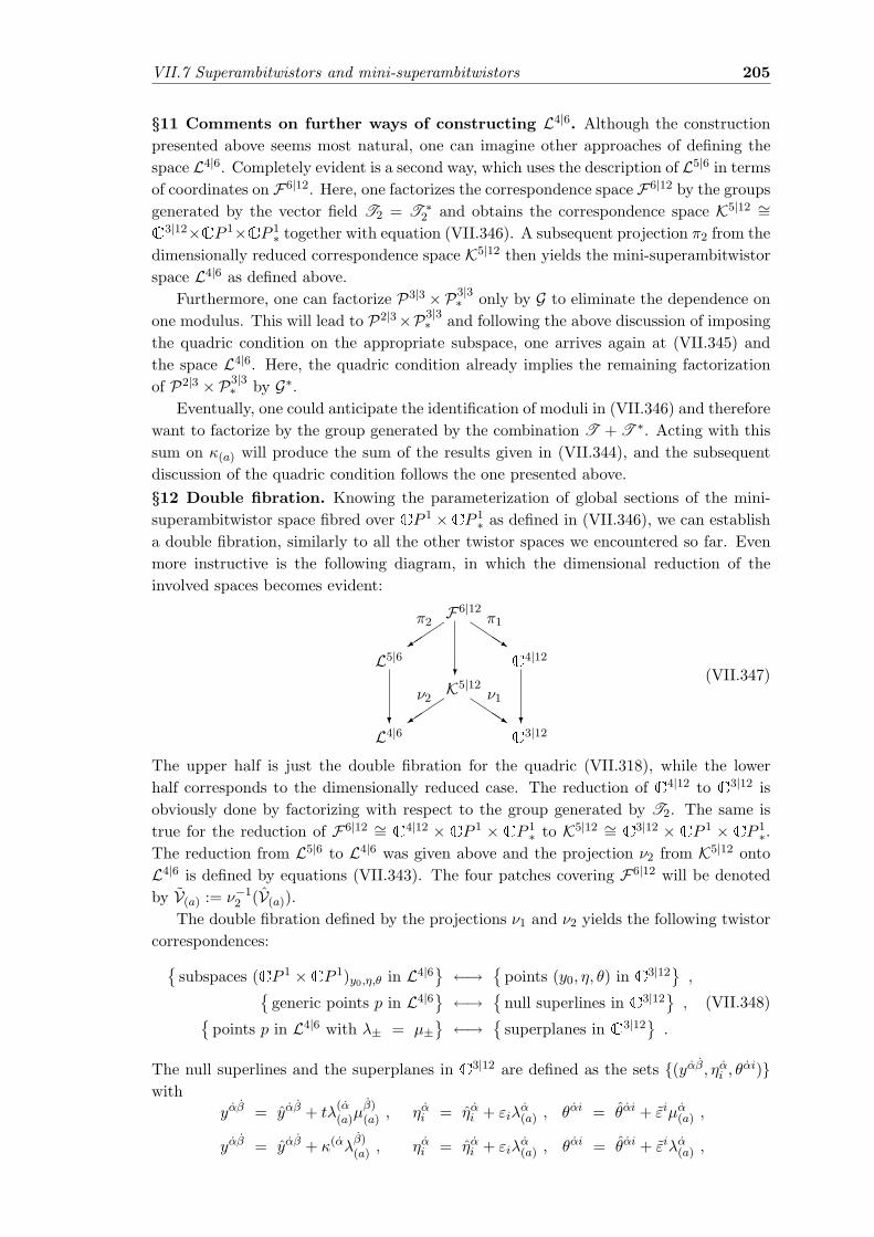
VII.7 Superambitwistors and mini-superambitwistors 205
§11 Comments on further ways of constructing L4|6. Although the constructionpresented above seems most natural, one can imagine other approaches of defining thespace L4|6. Completely evident is a second way, which uses the description of L5|6 in termsof coordinates on F6|12. Here, one factorizes the correspondence space F6|12 by the groupsgenerated by the vector field T2 = T ∗
2 and obtains the correspondence space K5|12 ∼=C3|12×CP 1×CP 1
∗ together with equation (VII.346). A subsequent projection π2 from thedimensionally reduced correspondence space K5|12 then yields the mini-superambitwistorspace L4|6 as defined above.
Furthermore, one can factorize P3|3 ×P3|3∗ only by G to eliminate the dependence on
one modulus. This will lead to P2|3×P3|3∗ and following the above discussion of imposing
the quadric condition on the appropriate subspace, one arrives again at (VII.345) andthe space L4|6. Here, the quadric condition already implies the remaining factorizationof P2|3 ×P3|3
∗ by G∗.Eventually, one could anticipate the identification of moduli in (VII.346) and therefore
want to factorize by the group generated by the combination T + T ∗. Acting with thissum on κ(a) will produce the sum of the results given in (VII.344), and the subsequentdiscussion of the quadric condition follows the one presented above.§12 Double fibration. Knowing the parameterization of global sections of the mini-superambitwistor space fibred over CP 1 ×CP 1
∗ as defined in (VII.346), we can establisha double fibration, similarly to all the other twistor spaces we encountered so far. Evenmore instructive is the following diagram, in which the dimensional reduction of theinvolved spaces becomes evident:
L4|6
L5|6
C3|12
C4|12
K5|12
F6|12
´´+
QQQs
´´+
QQQs
? ?
?
π2 π1
ν2 ν1
(VII.347)
The upper half is just the double fibration for the quadric (VII.318), while the lowerhalf corresponds to the dimensionally reduced case. The reduction of C4|12 to C3|12 isobviously done by factorizing with respect to the group generated by T2. The same istrue for the reduction of F6|12 ∼= C4|12 × CP 1 × CP 1
∗ to K5|12 ∼= C3|12 × CP 1 × CP 1∗.
The reduction from L5|6 to L4|6 was given above and the projection ν2 from K5|12 ontoL4|6 is defined by equations (VII.343). The four patches covering F6|12 will be denotedby V(a) := ν−1
2 (V(a)).The double fibration defined by the projections ν1 and ν2 yields the following twistor
correspondences:
subspaces (CP 1 ×CP 1)y0,η,θ in L4|6 ←→ points (y0, η, θ) in C3|12
,
generic points p in L4|6 ←→ null superlines in C3|12
,
points p in L4|6 with λ± = µ± ←→
superplanes in C3|12
.
(VII.348)
The null superlines and the superplanes in C3|12 are defined as the sets (yαβ, ηαi , θαi)
withyαβ = yαβ + tλ
(α(a)µ
β)(a) , ηα
i = ηαi + εiλ
α(a) , θαi = θαi + εiµα
(a) ,
yαβ = yαβ + κ(αλβ)(a) , ηα
i = ηαi + εiλ
α(a) , θαi = θαi + εiλα
(a) ,

206 Twistor Geometry
where t, κα, εi and εi are an arbitrary complex number, a complex commuting two-spinorand two three-vectors with Graßmann-odd components, respectively. Note that in thelast line, λα± = µα±, and we could also have written
(yαβ, ηαi , θαi) with yαβ = yαβ +κ(αµ
β)(a) , ηα
i = ηαi +εiµ
α(a) , θαi = θαi + εiµα
(a) .
The vector fields spanning the tangent spaces to the leaves of the fibration ν2 are forgeneric values of µ± and λ± given by
W (a) := µα(a)λ
β(a)∂(αβ) ,
Di(a) := λβ
(a)Diβ
:= λβ(a)
(∂
∂ηβi
+ θαi∂(αβ)
),
D(a)i := µα
(a)Dαi := µα(a)
(∂
∂θαi+ ηβ
i ∂(αβ)
),
(VII.349)
where the derivatives ∂(αβ) have been defined in (IV.77) and (IV.78). At µ± = λ±,however, the fibres of the fibration L4|6 over CP 1 × CP 1
∗ loose one bosonic dimension.As the space K5|12 is a manifold, this means that this dimension has to become tangentto the projection ν2. In fact, one finds that over CP 1
∆, besides the vector fields given in(VII.349), also the vector fields
W±β
= µα±∂(αβ) = λα
±∂(αβ) (VII.350)
annihilate the coordinates on L4|6. Therefore, the leaves to the projection ν2 : K5|12 →L4|6 are of dimension 2|6 for µ± = λ± and of dimension 1|6 everywhere else.§13 Real structure on L4|6. Quite evidently, a real structure on L4|6 is inherited fromthe one on L5|6, and we obtain directly from (VII.325) the action of τM on P2|4 × P2|4
∗ ,which is given by
τM (w1±, λ±α , η±i ; v1
±, µ±α , θi±) :=
(−v1±, µ±α , θi±;−w1±, λ±α , η±i
). (VII.351)
This action descends in an obvious manner to L4|6, which leads to a real structure onthe moduli space C3|12 via the double fibration (VII.347). Thus, we have as the resultingreality condition
yαβ0 = −yβα
0 and ηαi = θαi , (VII.352)
and the identification of the bosonic moduli yαβ with the coordinates on R3 reads as
y110 = −ix0 − ix3 , y12
0 = y210 = −ix1 , y22
0 = −ix0 + ix3 . (VII.353)
The reality condition τM (·) = · is indeed fully compatible with the condition (VII.345)which reduces P2|4 × P2|4
∗ to L4|6. The base space CP 1 × CP 1∗ of the fibration L4|6 is
reduced to a single sphere S2 with real coordinates 12(λ±+µ±) = 1
2(λ±+ λ±) and 12i(λ±−
µ±) = 12i(λ± − λ±), while the diagonal CP 1
∆ is reduced to a circle S1∆ parameterized by
the real coordinates 12(λ± + λ±). The τM -real sections of L4|6 have to satisfy w1± =
τM (w1±) = v1±. Thus, the fibres of the fibration L4|6 → CP 1×CP 1∗, which are of complex
dimension 2|6 over generic points in the base and complex dimension 1|6 over CP 1∆,
are reduced to fibres of real dimension 2|6 and 1|6, respectively. In particular, notethat θi±η±i = η±i θi± = −θi±η±i is purely imaginary and therefore the quadric condition(VII.345) together with the real structure τM implies that w1± = v1± = w1± + 2θi±η±i forλ± = µ± = λ±. Thus, the body
w1± of w1± is purely real and we have w1± =
w1± − θi±η±i
and v1± =w1± + θi±η±i on the diagonal S1
∆.

VII.7 Superambitwistors and mini-superambitwistors 207
§14 Interpretation of the involved real geometries. For the best-known twistor cor-respondences, i.e. the correspondence (VII.45), its dual and the correspondence (VII.129),there is a nice description in terms of flag manifolds, see e.g. the diagrams (VII.74),(VII.75) and (VII.132) as well as the discussion in [284]. For the spaces involved in thetwistor correspondences including mini-twistor spaces, one has a similarly nice interpreta-tion after restricting to the real situation. For simplicity, we reduce our considerations tothe bodies33 of the involved geometries, as the extension to corresponding supermanifoldsis quite straightforward.
Let us first discuss the double fibration for the mini-twistor space, cf. (VII.275),
P2|N C3|2N
K5|2Nν2 ν1¡¡ª
@@R
(VII.354)
and assume that we have imposed a suitable reality condition on the sections of P2|N →CP 1, the details of which are not important. We follow again the usual discussion of thereal case and leave the coordinates on the sphere complex.
As correspondence space on top of the doublefibration, we have thus the space R3×S2, whichwe can understand as the set of oriented lines34
in R3 with one marked point. Clearly, the pointof such a line is given by an element of R3, andthe direction of this line in R3 is parameterizedby a point on S2. The mini-twistor space P2 ∼=O(2) now is simply the space of all lines in R3
[126]. Similarly to the case of flag manifolds,the projections ν1 and ν2 in (VII.354) become therefore obvious. For ν1, simply dropthe line and keep the marked point. For ν2, drop the marked point and keep the line.Equivalently, we can understand ν2 as moving the marked point on the line to its shortestpossible distance from the origin. This leads to the space TS2 ∼= O(2), where the S2
parameterizes again the direction of the line, which can subsequently be still movedorthogonally to this direction, and this freedom is parameterized by the tangent planesto S2, which are isomorphic to R2.
Now in the case of the fibration which is in-cluded in (VII.347), we impose the reality condi-tion (VII.351) on the fibre coordinates of L4. Inthe real case, the correspondence space K5 be-comes the space R3 × S2 × S2 and this is thespace of two oriented lines in R3 intersecting ina point. More precisely, this is the space of twooriented lines in R3 each with one marked point,for which the two marked points coincide. The
projections ν1 and ν2 in (VII.347) are then interpreted as follows. For ν1, simply drop thetwo lines and keep the marked point. For ν2, fix one line and move the marked point (theintersection point) together with the second line to its shortest distance to the origin.
33i.e. drop the fermionic directions34not only the ones through the origin

208 Twistor Geometry
Thus, the space L4 is the space of configurations in R3, in which a line has a commonpoint with another line at its shortest distance to the origin.
Let us summarize all the above findings in the following table:
Space Relation to R3
R3 marked points in R3
R3 × S2 oriented lines with a marked point in R3
P2 ∼= O(2) oriented lines in R3 (with a marked point at shortest dis-tance to the origin.)
R3 × S2 × S2 two oriented lines with a common marked point in R3
L4 two oriented lines with a common marked point at shortestdistance from one of the lines to the origin in R3
§15 Remarks concerning a topological B-model on L4|6. The space L4|6 is notwell-suited as a target space for a topological B-model since it is not a (Calabi-Yau)manifold. However, one clearly expects that it is possible to define an analogous modelsince, if we assume that the conjecture in [202] is correct, such a model should simplybe the mirror of the mini-twistor string theory considered in [63]. This model wouldfurthermore yield some holomorphic Chern-Simons type equations of motion. The latterequations would then define holomorphic L4|6-bundles by an analogue of a holomorphicstructure. These bundles will be introduced in section 4.3 and in our discussion, theysubstitute the holomorphic vector bundles.
Interestingly, the space L4|6 has a property which comes close to vanishing of a firstChern class. Recall that for any complex vector bundle, its Chern classes are Poincaredual to the degeneracy cycles of certain sets of sections (this is a Gauß-Bonnet formula).More precisely, to calculate the first Chern class of a rank r vector bundle, one considersr generic sections and arranges them into an r× r matrix L. The degeneracy loci on thebase space are then given by the zero locus of det(L). Clearly, this calculation can betranslated directly to L4|6.
We will now show that L4|6 and L5|6 have equivalent degeneracy loci, i.e. they areequal up to a principal divisor, which, if we were speaking of ordinary vector bundles,would not affect the first Chern class. Our discussion simplifies considerably if we restrictour attention to the bodies of the two supertwistor spaces and put all the fermioniccoordinates to zero. Instead of the ambitwistor spaces, it is also easier to consider thevector bundles P3×P3∗ and P2×P2∗ over CP 1×CP 1
∗, respectively, with the appropriatelyrestricted sets of sections. Furthermore, we will stick to our inhomogeneous coordinatesand perform the calculation only on the patch U(1), but all this directly translates intohomogeneous, patch-independent coordinates. The matrices to be considered are
LL5 =
x1α1 λ+
α x1α2 λ+
α x1α3 λ+
α x1α4 λ+
α
x2α1 λ+
α x2α2 λ+
α x2α3 λ+
α x2α4 λ+
α
xα11 µ+
α xα12 µ+
α xα13 µ+
α xα14 µ+
α
xα21 µ+
α xα22 µ+
α xα23 µ+
α xα24 µ+
α
, LL4 =
yαβ
1 λ+α λ+
βyαβ2 λ+
α λ+
β
yαβ1 µ+
α µ+
βyαβ2 µ+
α µ+
β
,
and one computes the degeneracy loci for generic moduli to be given by the equations
(λ+ − µ+)2 = 0 and (λ+ − µ+)(λ+ − %+) = 0 (VII.355)

VII.7 Superambitwistors and mini-superambitwistors 209
on the bases of L5 and L4, respectively. Here, %+ is a rational function of µ+ and thereforeit is obvious that both degeneracy cycles are equivalent.
When dealing with degenerated twistor spaces, one usually retreats to the correspon-dence space endowed with some additional symmetry conditions [195]. It is conceivablethat a similar procedure will help to define the topological B-model in our case. Also,defining a suitable blow-up of L4|6 over CP 1
∆ could be the starting point for finding anappropriate action.
VII.7.4 The Penrose-Ward transform using mini-ambitwistor spaces
§16 L4|6-bundles. Because the mini-superambitwistor space is only a fibration and not amanifold, there is no notion of holomorphic vector bundles over L4|6. However, our spaceis close enough to a manifold to translate all the necessary terms in a simple manner.
Let us fix the covering U of the total space of the fibration L4|6 to be given bythe patches V(a) introduced above. Furthermore, define S to be the sheaf of smoothGL(n,C)-valued functions on L4|6 and H to be its subsheaf consisting of holomorphicGL(n,C)-valued functions on L4|6, i.e. smooth and holomorphic functions which dependonly on the coordinates given in (VII.343) and λ(a), µ(a).
We define a complex L4|6-bundle of rank n by a Cech 1-cocycle fab ∈ Z1(U, S) onL4|6 in full analogy with transition functions defining ordinary vector bundles, see sectionII.2.3. If the 1-cocycle is an element of Z1(U, H), we speak of a holomorphic L4|6-bundle.Two L4|6-bundles given by Cech 1-cocycles fab and f ′ab are called topologically equi-valent (holomorphically equivalent) if there is a Cech 0-cochain ψa ∈ C0(U, S) (a Cech0-cochain ψa ∈ C0(U, H)) such that fab = ψ−1
a f ′abψb. An L4|6-bundle is called trivial(holomorphically trivial) if it is topologically equivalent (holomorphically equivalent) tothe trivial L4|6-bundle given by fab = 1ab.
In the corresponding discussion of Cech cohomology on ordinary manifolds, one canachieve independence of the covering if the patches of the covering are all Stein manifolds.An analogous argument should be also applicable here, but for our purposes, it is enoughto restrict to the covering U.
Besides the Cech description, it is also possible to introduce an equivalent Dolbeaultdescription, which will, however, demand an extended notion of Dolbeault cohomologyclasses.§17 The Penrose-Ward transform. With the double fibration contained in (VII.347),it is not hard to establish the corresponding Penrose-Ward transform, which is essentiallya dimensional reduction of the four-dimensional case presented in section 4.1.
On L4|6, we start from a trivial rank n holomorphic L4|6-bundle defined by a 1-cocycle fab which becomes a holomorphically trivial vector bundle upon restriction toany subspace (CP 1 ×CP 1)y,η,θ→L4|6. The pull-back of the L4|6-bundle along ν2 is thevector bundle E with transition functions ν∗2fab satisfying by definition
W (a)ν∗2fab = Di(a)ν
∗2fab = D
(a)i ν∗2fab = 0 , (VII.356)
at generic points of L4|6 and for λ± = µ±, we have
W(a)α ν∗2fab = Di
(a)ν∗2fab = D
(a)i ν∗2fab = 0 . (VII.357)
Restricting the bundle E to a subspace (CP 1×CP 1)y,η,θ→L4|6 ⊂ F5|12 yields a splittingof the transition function ν∗2fab
ν∗2fab = ψ−1a ψb , (VII.358)

210 Twistor Geometry
where ψa are again GL(n,C)-valued functions on V(a) which are holomorphic. Fromthis splitting together with (VII.356), one obtains at generic points of L4|6 (we will discussthe situation over CP 1
∆ shortly) that
ψaDi(a)ψ
−1a = ψbD
i(a)ψ
−1b =: λα
(a)Aiα ,
ψaD(a)i ψ−1
a = ψbD(a)i ψ−1
b =: µα(a)Aαi ,
ψaW(a)ψ−1
a = ψbW(a)ψ−1
b =: µα(a)λ
β(a)Bαβ ,
(VII.359)
where Bαβ is a superfield which decomposes into a gauge potential and a Higgs field Φ:
Bαβ := A(αβ) + i2εαβΦ . (VII.360)
The zeroth order component in the superfield expansion of Φ will be the seventh realscalar joining the six scalars of N = 4 SYM in four dimensions, which are the zerothcomponent of the superfield Φij defined in
Dαi +Aαi, Dβj +Aβj =: −2εαβΦij . (VII.361)
Thus, as mentioned above, the Spin(7) R-symmetry group of N = 8 SYM theory in threedimensions will not be manifest in this description.
The equations (VII.359) are equivalent to the linear system
µα(a)λ
β(a)(∂(αβ) + Bαβ)ψa = 0 ,
λα(a)(D
iα + Ai
α)ψa = 0 ,
µα(a)(Dαi +Aαi)ψa = 0 .
(VII.362)
To discuss the corresponding compatibility conditions, we introduce the following differ-ential operators:
∇iα := Di
α + Aiα , ∇αi := Dαi +Aαi ,
∇αβ := ∂(αβ) + Bαβ .(VII.363)
We thus arrive at
∇iα, ∇j
β+ ∇i
β, ∇j
α = 0 , ∇αi,∇βj+ ∇βi,∇αj = 0 ,
∇αi, ∇j
β − 2δj
i∇αβ = 0 ,(VII.364)
and one clearly sees that equations (VII.364) are indeed equations (VII.333) after a di-mensional reduction C4 → C3 and defining Φ := A2. (Recall that we are reducing thecoordinates by x2.) As it is well known, the supersymmetry (and the R-symmetry) ofN = 4 SYM theory are enlarged by this dimensional reduction and we therefore obtainedindeed N = 8 SYM theory on C3.
Let us now examine how the special case λ± = µ± fits into the picture. One im-mediately notes that a transition function ν∗2fab, which satisfies (VII.356) is of the form
fab = fab(yαβλ(a)α λ
(a)
β, yαβµ
(a)α µ
(a)
β, λ
(a)α , µ
(a)α ) , (VII.365)
and thus the condition (VII.357) is obviously fulfilled for λ± = µ±. This implies inparticular that for λ± = µ±, nothing peculiar happens, and it suffices to consider thelinear system (VII.362).
VII.7 Superambitwistors and mini-superambitwistors 211
Following the above analysis in a straightforward manner for λ± = µ±, one arrives at alinear system which contains singular operators on CP 1
∆ and the compatibility conditionsof this system cannot be pushed forward from the correspondence space K5|12 down toC3|12. As mentioned above, we can ignore this point, as it will be equivalent to consideringthe linear system (VII.362) over CP 1
∆.To sum up, we obtained a correspondence between holomorphic L4|6-bundles which
become holomorphically trivial vector bundles upon reduction to any subspace (CP 1 ×CP 1)y,η,θ→L4|6 and solutions to the three-dimensional N = 8 SYM equations. As thiscorrespondence arises by a dimensional reduction of a correspondence which is one-to-one, it is rather evident that also in this case, we have a bijection between both theholomorphic L4|6-bundles and the solutions after factorizing with respect to holomorphicequivalence and gauge equivalence, respectively.
§18 Yang-Mills-Higgs theory in three dimensions. One can translate the discussionof the ambitwistor space in VII.3.3 to the three-dimensional situation, giving rise toa Penrose-Ward transform between holomorphic L4 bundles and the Yang-Mills-Higgsequations. First of all, recall from section IV.2.5, §30 the appropriate Yang-Mills-Higgsequations obtained by dimensional reduction are
∇(αβ)F(αβ)(γδ) = [φ,∇(γδ)φ] and 4φ := ∇(αβ)∇(αβ)φ = 0 , (VII.366)
while the self-dual and anti-self-dual Yang-Mills equations correspond after the dimen-sional reduction to two Bogomolny equations which read
F(αβ)(γδ) = ε(αβ)(γδ)(εζ)∇(εζ)φ and F(αβ)(γδ) = −ε(αβ)(γδ)(εζ)∇(εζ)φ , (VII.367)
respectively. Using the decomposition F(αβ)(γδ) = εαγfβδ + εβδfαγ , the above two equa-tions can be simplified to
fαβ = i2∇(αβ)φ and fαβ = − i
2∇(αβ)φ . (VII.368)
Analogously to the four-dimensional case, we start from a vector bundle E over the spaceC3 ×C3 with coordinates p(αβ) and q(αβ); additionally we introduce the coordinates
y(αβ) = 12(p(αβ) + q(αβ)) and h(αβ) = 1
2(p(αβ) − q(αβ)) (VII.369)
and a gauge potential
A = Ap
(αβ)dp(αβ) + Aq
(αβ)dq(αβ) = Ay
(αβ)dy(αβ) + Ah
(αβ)dh(αβ) (VII.370)
on E. The differential operators we will consider in the following are obtained fromcovariant derivatives by dimensional reduction and take, e.g., the shape
∇y
αβ=
∂
∂y(αβ)+ [Ay
(αβ)+ i
2εαβφy, · ] . (VII.371)
We now claim that the Yang-Mills-Higgs equations (VII.366) are equivalent to the equa-tions
[∇p
αβ,∇p
γδ] = ∗[∇p
αβ,∇p
γδ] +O(h2) ,
[∇q
αβ,∇q
γδ] = − ∗ [∇q
αβ,∇q
γδ] +O(h2) ,
[∇p
αβ,∇q
γδ] = O(h2) ,
(VII.372)

212 Twistor Geometry
where we can use ∗[∇p,q
αβ,∇p,q
γδ] = εαβγδεζ∇εζ
p,qφp,q. These equations can be simplified inthe coordinates (y, h) to equations similar to (VII.151), which are solved by the fieldexpansion
Ah(αβ)
= −12F y,0
(αβ)(γδ)h(γδ) − 1
3h(γδ)∇y,0
(γδ)ε(αβ)(εζ)(στ)(∇
(στ)y,0 φ)h(εζ) ,
φh = 12∇y,0
(γδ)φy,0h(γδ) + 1
6h(γδ)∇y,0
(γδ)ε(αβ)(εζ)(στ)F y,0
(εζ)(στ)h(αβ) ,
Ay
(αβ)= Ay,0
(αβ)− ε(αβ)(εζ)(στ)(∇
(στ)y,0 φy,0)h(εζ) − 1
2h(γδ)∇y,0
(γδ)(F y,0
(αβ)(εζ))h(εζ) ,
φy = φy,0 + 12ε(αβ)(εζ)(στ)F y,0
(εζ)(στ)h(αβ) + 1
2h(γδ)∇y,0
(γδ)(∇(αβ)φ
y,0)h(αβ) ,
(VII.373)
if and only if the Yang-Mills-Higgs equations (VII.366) are satisfied.
Thus, solutions to the Yang-Mills-Higgs equations (VII.366) correspond to solutionsto equations (VII.372) on C3 × C3. Recall that solutions to the first two equationsof (VII.372) correspond in the twistor description to holomorphic vector bundles overP2×P2∗ . Furthermore, the expansion of the gauge potential (VII.373) is an expansion ina second order infinitesimal neighborhood of diag(C3×C3). As we saw in the constructionof the mini-superambitwistor space L4|6, the diagonal for which h(αβ) = 0 corresponds toL4 ⊂ P2×P2∗ . The neighborhoods of this diagonal will then correspond to sub-thickeningsof L4 inside P2 ×P2∗ , i.e. for µ± = λ±, we have the additional nilpotent coordinate ξ. Inother words, the sub-thickening of L4 in P2 ×P2∗ is obtained by turning one of the fibercoordinates of P2 × P2 over CP 1
∆ into a nilpotent even coordinate (in a suitable basis).Then we can finally state the following:
Gauge equivalence classes of solutions to the three-dimensional Yang-Mills-Higgsequations are in one-to-one correspondence with gauge equivalence classes of holomorphicL4-bundles over a third order sub-thickening of L4, which become holomorphically trivialvector bundles when restricted to a CP 1 ×CP 1 holomorphically embedded into L4.
VII.8 Solution generating techniques
In this section, we will discuss solution generating techniques which are related to thetwistorial description of field theories.
The Atiyah-Drinfeld-Hitchin-Manin (ADHM) construction of instantons [13] reducesthe self-duality equations to a simple set of matrix equations. This construction has beenshown to be complete, i.e. all instanton solutions can be obtained by this algorithm. Theoriginal idea was to find an instanton bundle over P3 (a topologically trivial holomorphicvector bundle, which becomes holomorphically trivial upon restriction to any CP 1
x ⊂ P3)from a so-called monad. Nevertheless, a very nice interpretation in terms of D-braneconfigurations has been found later on [295, 84, 85], see also [83, 274]. Furthermore,supersymmetric extensions of the ADHM construction have been proposed [256, 282].
The corresponding reduction to the three-dimensional Bogomolny equations is givenby the Nahm construction [200] with a D-brane interpretation developed in [75]. Acorresponding superextension was proposed in [176], and we will present this extensionin section VII.8.4.
We will present further solution generating techniques in section VIII.3.2.

VII.8 Solution generating techniques 213
VII.8.1 The ADHM construction from monads
In discussing the ADHM construction from monads, we follow essentially the presenta-tions in [284] and [94]. The technique of obtaining vector bundles from monads stemsoriginally from Horrocks [132], see also [12].§1 Monads. A monad M over a manifold M is a triple of vector bundles A, B,C overM , which fits into the sequence of vector bundles
Aα−→ B
β−→ C , (VII.374)
and thus the linear maps α and β satisfy βα = 0. The vector bundle E = kerβ/imα iscalled the cohomology of the monad.
The rank and the total Chern class of the cohomology E of the monad M constructedabove can be derived from the corresponding data of the triple A,B,C via the formulæ
rkE = rkB − rkA− rkC ,
c(E) = c(B)c(A)−1c(C)−1 .(VII.375)
§2 Annihilator. The annihilator U0 ⊂ V of a subspace U of a symplectic vector space35
V is given by those vectors v ∈ V , which vanish upon pairing with any element of U andapplying the symplectic form:
U0 := v ∈ V |ω(v, u) = 0 for all u ∈ U . (VII.376)
§3 The instanton monad. Let us now construct a monad M, which yields an instantonbundle as its cohomology. For simplicity, we will restrict ourselves to the gauge groupSU(2), but via embeddings, it is possible to generalize this discussion to gauge groupsSU(n), SO(n) and Sp(n).
Note that by introducing a symplectic form ω on a vector bundle B, B can be identifiedwith its own dual. Furthermore, A will be dual to C and α to β. Thus, we can reducethe data defining our monad M to A, (B,ω) and α. For our construction, we choose A
to be Ok(−1) over CP 3 and B is the trivial bundle C2k+2 → CP 3.It now remains to specify α. For this, take two complex vector spaces V = C2k+2 and
W = Ck with a symplectic form ω on V , on both of which we have antilinear maps τ ,with τ2
W = 1 (a complex conjugation) and τ2V = −1 (induced from the real structure on
CP 3), the latter being compatible with the symplectic form ω: ω(τv1, τv2) = ω(v1, v2)and the induced Hermitian form h(v1, v2) = ω(v1, τv2) for v1,2 ∈ V shall be positivedefinit. Additionally, we assume a map
α : W → V with α = AiZi = Aαλα + Aαωα , (VII.377)
where (Zi) := (ωα, λα) will become the homogeneous coordinates on the twistor spaceCP 3 and Aα, Aα are constant linear maps from W to V . The map α satisfies the com-patibility condition τα(Z)w = α(τZ)τw with the maps τ . Since α is linear in Z, wecan also see it as a homomorphism of vector bundles α : W (−1) → V × CP 3, whereW (−1) = W ⊗OCP 3(−1). From the map α∨ : V ∨ = V → W∨, we obtain the monad M
W (−1) α−→ V ×CP 3 α∨−→ W∨(1) , (VII.378)
35A symplectic vector space is a vector space equipped with a symplectic form ω. That is, ω is a
nondegenerate, skew-symmetric bilinear form.

214 Twistor Geometry
where W∨(1) is the space W ⊗ (OCP 3(−1))∨.We impose now two additional conditions on the linear map α. First, the space
UZ := αW is of dimension k and second, for all Z 6= 0, UZ is a subset of U0Z . The latter
condition is automatically satisfied for k = 1. For k > 1, this amounts to the matrixequation αT ωα = 0. The instanton bundle over36 CP 3 is then given by the resultingcohomology
EZ := U0Z/UZ (VII.379)
of M. Since both U0Z and UZ are independent of the scaling, we have EZ = EtZ and
therefore the family of all EZ is indeed a vector bundle E over CP 3. In particular, sincedimUZ = k and dimU0
Z = k + 2, we have dimEZ = 2, which is the desired result foran SU(2)-instanton bundle. The symplectic form ω on V induces a symplectic form ω onEZ , which renders the latter bundles structure group to SL(2,C).
One can verify that the bundle E constructed in this manner is in fact an instantonbundle [12], and via the Penrose-Ward transform, one obtains the corresponding self-dualgauge potential.
§4 The picture over the moduli space. Instead of constructing the vector spacesV and W over the twistor space CP 3 fibered over S4, we can discuss them directlyover the space S4. To this end, define V and W as before and choose τ to be thecomplex conjugation on W . The symplectic form ω on V is given by a skew-symmetrictri-band matrix of dimension (2k + 2)× (2k + 2) with entries ±1. The reality conditionτα(Z)w = α(τZ)τw on the map α can now be restated in the following way: Let usdenote the components of the matrix B by Bα
i,j . Then for fixed values of m, n, the2× 2-matrix Bα
2m+β−1,nshould be a quaternion. Applying the same argument to C, we
arrive at a representation of the map α in terms of a (k + 1) × k-dimensional matrix ofquaternions
∆ = A− Cx . (VII.380)
The remaining condition that α(Zi)W should be of dimension k for Zi 6= 0 amounts to thefact that ∆(x)∆(x) is nonsingular and real for each x, where ∆ is the conjugate transposeof ∆. This condition is equivalent to the so-called ADHM equations, which will arise inthe following section. One can easily “supersymmetrize” the above considerations, byconsidering a supertwistor space CP 3|N and adding appropriate linear terms to (VII.377)and (VII.380).
VII.8.2 The ADHM construction in the context of D-branes
§5 The D5-D9-brane system. As stated in the introduction to this section, the ADHMalgorithm for constructing instanton solutions has found a nice interpretation in thecontext of string theory. We start from a configuration of k D5-branes bound to a stackof n D9-branes, which – upon dimensional reduction – will eventually yield a configurationof k D(-1)-branes inside a stack of n D3-branes.
§6 D5-D5 strings. From the perspective of the D5-branes, the N = 2 supersymmetryof type IIB superstring theory is broken down to N = (1, 1) on the six-dimensionalworldvolume of the D5-brane, which is BPS. The fields in the ten-dimensional Yang-Mills multiplet are rearranged into an N = 2 vector multiplet (φa, Aαα, χi
α, µαi ), where
36Usually in this discussion, one considers the twistor space CP 3 of S4, and imposes the restrictions
only for Zi 6= 0.

VII.8 Solution generating techniques 215
the indices i = 1, . . . , 4, a = 1, . . . 6 and α, α = 1, 2 label the representations of theLorentz group SO(5, 1) ∼ SU(4) and the R-symmetry group SO(4) ∼ SU(2)L × SU(2)R,respectively. Thus, φ and A denote bosons, while χ and µ refer to fermionic fields.
Note that the presence of the D9-branes will furtherbreak supersymmetry down to N = (0, 1) and there-fore the above multiplet splits into the vector mul-tiplet (φa, µ
αi ) and the hypermultiplet (Aαα, χi
α). Inthe following, we will discuss the field theory on theD5-branes in the language of N = (0, 1) supersym-metry.
Let us now consider the vacuum moduli space ofthis theory which is called the Higgs branch. This isthe sector of the theory, where the D-field, i.e. theauxiliary field for the N = (0, 1) vector multiplet,vanishes37. Therefore, we can restrict our analysis inthe following to a few terms of the action. From theYang-Mills part describing the vector multiplet, wehave the contribution 4π2α′2
∫d6x tr k
12D2
µν , wherewe also introduce the notation Dµν = tr 2(~σσµν) · ~D. The hypermultiplet leads to anadditional contribution of
∫d6x tr ki ~D · ~σα
βAαβAαα. Note that we will use a bar insteadof the dagger to simplify notation. However, this bar must not be confused with complexconjugation.
§7 D5-D9 strings. It remains to include the contributions from open strings havingone end on a D5-brane and the other one on a D9-brane. These additional degrees offreedom are aware of both branes and therefore form hypermultiplets under N = (0, 1)supersymmetry. One of the hypermultiplets is in the (k,n) representation of U(k)×U(n),while the other one transforms as (k, n). We denote them by (wα, ψi) and (wα, ψi),where wα and wα and ψi and ψi denote four complex scalars and eight Weyl spinors,respectively. The contribution to the D-terms is similar to the hypermultiplet consideredabove:
∫d6x tr ki ~D · ~σα
βwβwα.
§8 The D-flatness condition. Collecting all the (algebraic) contributions of the D-fieldto the action and varying them yields the equations of motion
α′2 ~D =i
16π2~σα
β(wβwα + AαβAαα) . (VII.381)
After performing the dimensional reduction of the D5-brane to a D(-1)-brane, the condi-tion that ~D vanishes is precisely equivalent to the ADHM constraints.
§9 The zero-dimensional Dirac operator. Spelling out all possible indices on ourfields, we have Aααpq and wupα, where p, q = 1, . . . , k denote indices of the representationk of the gauge group U(k) while u = 1, . . . , n belongs to the n of U(n). Let us introducethe new combinations of indices r = u⊕ p⊗α = 1, . . . , n + 2k together with the matrices
(arqα) =
(wuqα
Aααpq
), (aαr
q ) =(wα
qu Aααpq
)and (bβ
rq) =
(0
δαβδpq
), (VII.382)
37This is often referred to as the D-flatness condition.

216 Twistor Geometry
which are of dimension (n + 2k)× 2k, 2k× (n + 2k) and (n + 2k)× 2k, respectively. Nowwe are ready to define a (n + 2k) × 2k dimensional matrix, the zero-dimensional Diracoperator of the ADHM construction, which reads
∆rpα(x) = arpα + bαrpxαα , (VII.383)
and we put ∆αrp := (∆rpα)∗. Written in the new components (VII.382), the ADHM
constraints amounting to the D-flatness condition read ~σαβ(aβaα) = 0, or, more explicitly,
aαaβ + aβaα = 0 , (VII.384)
where we defined as usual aα = εαβ aβ. All further conditions, which are sometimes alsosummarized under ADHM constraints, are automatically satisfied due to our choice ofbαrp and the reality properties of our fields.
§10 Construction of solutions. The kernel of the zero-dimensional Dirac operatoris generally of dimension n, as this is the difference between its numbers of rows andcolumns. It is spanned by vectors, which can be arranged to a complex matrix Uru whichsatisfies
∆αrp Uru = 0 . (VII.385)
Upon demanding that the frame Uru is orthonormal, i.e. that U ruUrv = δuv, we can
construct a self-dual SU(n)-instanton configuration from
(Aαα)uv = U ru∂ααUrv . (VII.386)
Usually, one furthermore introduces the auxiliary matrix f via
f = 2(wαwα + (Aαα + xαα ⊗ 1k)2)−1 , (VII.387)
which fits in the factorization condition ∆αrp ∆rqβ = δα
β(f−1)pq. Note that the latter
condition is equivalent to the ADHM constraints (VII.384) arising from (VII.381). Thematrix f allows for an easy computation of the field strength
Fµν = 4Ubσµνf bU (VII.388)
and the instanton number
− 116π2
∫d4x tr nF 2
µν =1
16π2
∫d4x ¤2 tr n log f . (VII.389)
Note that the self-duality of Fµν in (VII.388) is evident from the self-duality property ofσµν .
VII.8.3 Super ADHM construction and super D-branes
§11 Superspace formulation of SYM theories. First, recall from section IV.2 thatone can formulate the equations of motion of N = 4 super Yang-Mills theory and self-dual Yang-Mills theory with arbitrary N both in terms of ordinary fields on R4 (or itscomplexification C4) and in terms of superfields on certain superspaces having R4 astheir body. For N = 4 SYM theory, the appropriate superspace is R4|16 (or C4|16),while for N -extended SDYM theory, one has to use R4|2N (or C4|2N ). One can find anEuler operator, which easily shows the equivalence of the superfield formulation with theformulation in terms of ordinary fields.

VII.8 Solution generating techniques 217
§12 Superbrane system. For the super ADHM construction, let us consider k D5|8-branes inside n D9|8-branes. To describe this scenario, it is only natural to extendthe fields arising from the strings in this configuration to superfields on C10|8 and theappropriate subspaces, respectively. In particular, we will extend the fields wα and Aαα
entering into the D-flatness condition in the purely bosonic setup to superfields livingon C6|8. However, since supersymmetry is broken down to four copies of N = 1 dueto the presence of the two stacks of D-branes, these superfields can only be linear inthe Graßmann variables. From the discussion in [120], we can then even state what thesuperfield expansion should look like:
wα =wα + ψiηiα and Aαα =
Aαα + χi
αηiα . (VII.390)
§13 Super ADHM equations. The D-flatness condition we arrive at after followingthe above discussion of the field theories involved in the D-brane configurations readsagain
α′2 ~D =i
16π2~σα
β(wβwα + AαβAαα) = 0 , (VII.391)
but here, all the fields are true superfields. After performing the dimensional reductionof the D9|8-D5|8-brane configuration to one containing D3|8- and D(-1|8)-branes, andarranging the resulting field content according to (VII.382), we can construct the zero-dimensional super Dirac operator
∆riα = ariα + bαrix
Rαα =
ariα + bα
rixRαα + cj
riηjα , (VII.392)
where (xααR , ηα
i ) are coordinates on the (anti-)chiral superspace C4|8. That is, from thepoint of view of the full superspace C4|16 with coordinates (xαα, θiα, ηα
i ), we have xααR =
xαα + θiαηαi . The ADHM constraints are now turned into the super ADHM constraints,
which were discussed in [256] for the first time, see also [7] for a related recent discussion.Explicitly, these super constraints (VII.384) read here
aα
a
β +aβ
aα = 0 ,
aαci − ci
aα = 0 , cicj − cjci = 0 . (VII.393)
The additional sign in the equations involving ci arises from ordering and extracting theGraßmann variables ηα
i as well as the definition ciηαi = ηα
i ci = −ciηαi .
§14 Construction of solutions. As proven in [256, 280], this super ADHM constructiongives rise to solutions to the N = 4 supersymmetrically extended self-dual Yang-Millsequations in the form of the super gauge potentials
Aαα = U∂ααU and A iα = UDi
αU , (VII.394)
where U and U are again zero modes of ∆ and ∆ and furthermore satisfy UU = 1.That is, the super gauge potentials in (VII.394) satisfy the constraint equations of N = 4self-dual Yang-Mills theory (IV.64).
One might be tempted to generalize the Dirac operator in (VII.392) to higher ordersin the Graßmann variables, but this is unnatural both from the point of view of brokensupersymmetry due to the presence of D-branes and from the construction of instantonbundles via monads (the original idea which gave rise to the ADHM construction). Be-sides this, higher powers of Graßmann variables will render the super ADHM equationsinsufficient for producing solutions to the self-dual Yang-Mills equations38. Note also
38In [82], a Dirac operator with higher powers is mentioned, but it is not used to obtain solutions in
the way we do.

218 Twistor Geometry
that this construction leads to solutions of the N = 4 SDYM equations, for which theHiggs fields tend to zero as x → ∞. Since the Higgs-fields describe the motion of theD3-brane in the ambient ten-dimensional space, this merely amounts to a choice of coor-dinates: The axes of the remaining six directions go through both “ends” of the stack ofD3-branes at infinity. For a discussion of the construction of solutions which do not tendto zero but to a constant value ∼ σ3 see [82] and references therein.
The fact that solutions to the N = 4 SDYM equations in general do not satisfy theN = 4 SYM equations does not spoil our interpretation of such solutions as D(-1|8)-branes, since in our picture, N = 4 supersymmetry is broken down to four copies ofN = 1 supersymmetry. Note furthermore that N = 4 SYM theory and N = 4 SDYMtheory can be seen as different weak coupling limits of one underlying field theory [297].
VII.8.4 The D-brane interpretation of the Nahm construction
Before presenting its super extension, let us briefly recollect the ordinary Nahm con-struction [200] starting from its D-brane interpretation [75] and [124], see also [274]. Forsimplicity, we restrict ourselves to the case of SU(2)-monopoles, but a generalization ofour discussion to gauge groups of higher rank is possible and rather straightforward.
§15 The D3-D1-brane system.We start in ten-dimensional typeIIB superstring theory with a pairof D3-branes extended in the di-rections 1, 2, 3 and located at x4 =±1, xM = 0 for M > 4. Considernow a bound state of these D3-branes with k D1-branes extend-ing along the x4-axis and endingon the D3-branes. As in the case of the ADHM construction, we can look at this config-uration from two different points of view.
From the perspective of the D3-branes, the effective field theory on their worldvolumeis N = 4 super Yang-Mills theory. The D1-branes bound to the D3-branes and endingon them impose a BPS condition, which amounts to the Bogomolny equations in threedimensions
DaΦ = 12εabcFbc , (VII.395)
where a, b, c = 1, 2, 3. The end of the D1-branes act as magnetic charges in the worldvol-ume of the D3-branes, and they can therefore be understood as magnetic monopoles [51],whose field configuration (Φ, Aa) satisfy the Bogomolny equations. These monopoles arestatic solutions of the underlying Born-Infeld action.
From the perspective of the D1-branes, the effective field theory is first N = (8, 8)super Yang-Mills theory in two dimensions, but supersymmetry is broken by the presenceof the two D3-branes to N = (4, 4). As before, one can write down the correspondingD-terms [274] and impose a D-flatness condition:
D =∂Xa
∂x4+ [A4, X
a]− 12εabc[Xb, Xc] + R = 0 , (VII.396)
where the Xa are the scalar fields corresponding to the directions in which the D3-branesextend. The R-term is proportional to δ(x4 ± 1) and allow for the D1-branes to end on

VII.8 Solution generating techniques 219
the D3-branes. They are related to the so-called Nahm boundary conditions, which wedo not discuss. The theory we thus found is simply self-dual Yang-Mills theory, reducedto one dimension.§16 Nahm equations. By imposing temporal gauge A4 = 0, we arrive at the Nahmequations
∂Xa
∂s− 1
2εabc[Xb, Xc] = 0 for − 1 < s < 1 , (VII.397)
where we substituted s = x4. From solutions to these (integrable) equations, we canconstruct the one-dimensional Dirac operator
∆αβ = (12)αβ ⊗ ∂
∂s+ σ(αβ)
a (xa −Xa) . (VII.398)
The equations (VII.397) are analogously to the ADHM equations the condition for ∆∆to commute with the Pauli matrices, or equivalently, to have an inverse f :
∆∆ = 12 ⊗ f−1 . (VII.399)
§17 Construction of solutions. The normalized zero modes U of the Dirac operator∆ satisfying
∆(s)U = 0 ,
∫ 1
−1ds U(s)U(s) = 1 (VII.400)
then give rise to solutions to the Bogomolny equations (VII.395) via the definitions
Φ(x, t) =∫ 1
−1ds U(s)sU(s) and Aa(x, t) =
∫ 1
−1ds U(s)∂aU(s) . (VII.401)
The verification of this statement is straightforward when using the identity
U(s)U(s′) = δ(s− s′)−−→∆(s)f(s, s′)←−∆(s′) . (VII.402)
Note that all the fields considered above stem from D1-D1 strings. The remaining D1-D3strings are responsible for imposing the BPS condition and the Nahm boundary conditionsfor the Xa at s = ±1.§18 Super Nahm construction. The superextension of the Nahm construction is ob-tained analogously to the superextension of the ADHM construction by extending theDirac operator (VII.398) according to
∆αβ = (12)αβ ⊗ ∂
∂s+ σ(αβ)
a (xa −Xa) + (η(αi χβ)i) . (VII.403)
The fields χαi are Weyl-spinors and arise from the D1-D1 strings. (More explicitly,consider a bound state of D7-D5-branes, which dimensionally reduces to our D3-D1-brane system. The spinor χαi is the spinor χi
α we encountered before when discussingthe N = (0, 1) hypermultiplet on the D5-brane.)

220 Twistor Geometry

Chapter VIII
Matrix Models
It is essentially three matrix models which received the most attention from string theo-rists during the last years. First, there is the Hermitian matrix model, which appeared inthe early nineties in the context of two-dimensional gravity and c = 1 non-critical stringtheory, see [103] and references therein. It experienced a renaissance in 2002 by the workof Dijkgraaf and Vafa [78]. Furthermore, there are the two matrix models which arerelated to dimensional reductions of ten-dimensional super Yang-Mills theory, the BFSSmatrix model [20] and the IKKT matrix model [140], see also [5]. The latter two areconjectured to yield non-perturbative and in particular background independent defini-tions of M-theory and type IIB superstring theory, respectively. The same aim underliesthe work of Smolin [262], in which the simplest possible matrix model, the cubic matrixmodel (CMM), was proposed as a fundamental theory.
In this chapter, we will furthermore present the results of [176], in which two pairs ofmatrix models were constructed in the context of twistor string theory.
VIII.1 Matrix models obtained from SYM theory
For the comparison with the twistor matrix models presented later, let us review someaspects of the BFSS and the IKKT matrix models. The motivation for both these modelswas to find a non-perturbative definition of string theory and M-theory, respectively.
VIII.1.1 The BFSS matrix model
In their famous paper [20], Banks, Fishler, Shenkar and Susskind conjectured that M-theory in the infinite momentum frame (IMF, see e.g. [34]) is exactly described by largeN supersymmetric matrix quantum mechanics.
§1 Matrix quantum mechanics. The Lagrangian for matrix quantum mechanics withMinkowski time is given by
L = tr(
12 Φ2 − U(Φ)
), (VIII.1)
where Φ is a Hermitian N × N matrix. This Lagrangian is invariant under time-independent SU(N) rotations. To calculate further, it is useful to decompose Φ intoeigenvalues and angular degrees of freedom by using Φ(t) = Ω†(t)Λ(t)Ω(t), where Λ(t)is a diagonal matrix with the eigenvalues of Φ(t) as its entries and Ω(t) ∈ SU(N). Wecan furthermore rewrite tr Φ2 = tr Λ2 + tr [Λ, ΩΩ†]2 and decompose ΩΩ† using symmet-ric, antisymmetric and diagonal generators with coefficients αij , βij and αi, respectively.After performing the trace, the Lagrangian reads as
L =∑
i
(12 λ2
i + U(λi))
+ 12
∑
i<j
(λi − λj)2(α2ij + β2
ij) . (VIII.2)

222 Matrix Models
The integration measure of the path integral is transformed to DΦ = DΩ∆2(Λ)Πidλi,where ∆(Λ) =
∏i<j(λi−λj) is the so-called Vandermonde determinant. The correspond-
ing Hamiltonian reads as
H = − 12β2∆(Λ)
∑
i
d2
dλ2i
∆(Λ) +∑
i
U(λi) +∑
i<j
Π2ij + Π2
ij
(λi − λj)2, (VIII.3)
where Πij and Πij are the momenta conjugate to αij and βij . For more details, see [153].§2 BFSS action. The action of the BFSS model, describing N D0-branes, can be ob-tained by dimensional reduction of 10-dimensional N = 1 super Yang-Mills theory withgauge group U(N) to 0 + 1 dimensions in temporal gauge A0 = 0:
S = 12g
∫dt
[tr XiXi + 2θT θ +
12
tr [Xi, Xj ]2 − 2θT γi[θ, Xi]]
. (VIII.4)
Here, the Xi are nine Hermitian N ×N matrices and θ is a Majorana-Weyl spinor. Notethat the bosonic part of the BFSS Lagrangian is a matrix quantum mechanics Lagrangian.Putting all the fermions to zero, one obtains the bosonic equations of motion
Xi = −[[Xi, Xj ], Xj ] . (VIII.5)
Restricting to the special class of classical (vacuum) solutions which satisfy [Xi, Xj ] =0, the matrices are simultaneously diagonalizable and for gauge group U(N) we can inter-pret such solutions as a stack of N D0-branes, whose positions in the normal directionsare given by the eigenvalues of the Xi.
The remaining classical solutions to (VIII.5) do not annihilate the positive-definitepotential term and are thus no vacuum solutions. They break supersymmetry, and inparticular, correspond to D0-branes, whose worldvolumes are smeared out in the normaldirections.§3 The BFSS model on a circle. To describe D0-branes in a spacetime, which has beencompactified in one direction normal to the worldvolume of the D0-branes, we considerinfinitely many copies of a D0-brane configuration and mod out the lattice symmetrygroup afterwards. A good reference here is [272].
To describe the copies of the D0-brane configuration, we extend the N×N -dimensionalmatrices Xi to ∞×∞-dimensional matrices Xi
nm which are divided into N ×N -dimen-sional blocks, specified by the indices n,m ∈ Z. We furthermore impose the conditionXmn = −X†
nm on the blocks. The new Lagrangian then reads
L =12g
[tr Xi
mnXinm +
12
tr (XimqX
jqn −Xj
mqXiqn)(Xi
nrXjrm −Xj
nrXirm)
]. (VIII.6)
The periodicity condition from compactifying the X1-direction on a circle with radiusR translates into the following conditions on the matrices Xi
mn:
Ximn = Xi
(m−1)(n−1), i > 1 (VIII.7)
X1mn = X1
(m−1)(n−1), m 6= n (VIII.8)
X1mm = X1
(m−1)(m−1) + 2πR1. (VIII.9)
The first equation renders all blocks on diagonals equal for i > 1, the second equationdoes the same for some of the diagonals of X1. The third equation shifts subsequent

VIII.1 Matrix models obtained from SYM theory 223
blocks on the principal diagonal for i = 1 by an amount of 2πR, the circumference of thecircle. Anti-Hermiticity of the Xi
mn implies furthermore (Xin)† = −Xi−n. We thus arrive
at
X1 =
. . ....
......
. . .· · · X1
0 − 2πR1 X11 X1
2 · · ·· · · X1
−1 X10 X1
1 · · ·· · · X1
−2 X1−1 X1
0 + 2πR1 · · ·. . .
......
.... . .
(VIII.10)
Rewriting the Lagrangian (VIII.6) in terms of Xin gives the description of D0-branes
moving in a compactified spacetime. Expansions around the classical vacuum [Xi, Xj ] = 0lead to the expected mass terms proportional to the distance of the branes plus thewinding contribution 2πRn, similarly to our discussion of T-duality in section V.2.3.
Note that this matrix quantum mechanics is automatically a second quantized for-malism as it allows for an arbitrary number of D0-branes. This analysis can also be easilygeneralized to more than one compact dimension [271].
§4 Reconstruction of spatial dimensions. Let us consider the following correspon-dence:
φ(x) =∑
n
φneinx/R ↔
...φ−1
φ0
φ1...
(VIII.11)
where R = 12πR . Then X1 is a matrix representation of the covariant derivative along the
compactified direction:
(i∂1 + A1(x))φ(x) ↔ X1 ~φ (VIII.12)
where A1(x) is a gauge potential whose Fourier modes are identified with X1n:
A1(x) =∑
n
A1neinx/R =
∑n
X1neinx/R. (VIII.13)
Here, the derivative leads to the inhomogeneous terms ∼ 2πn1 and the gauge field givesrise to the remaining components.
To return to the dual space, we can consider an analogous Fourier decomposition ofY i(x) =
∑n Xi
neinx/R, with which we can rewrite the BFSS Lagrangian as
L =∫
dx1
2πR
12g
[tr Y iY i + + tr A1A1 − tr (∂1Y
i − i[A1, Y i])2 +12
tr [Y i, Y j ]2]
.
By integrating over x1, we obtain again the Lagrangian (VIII.6).This result corresponds to T-duality in the underlying string theory and describes k
D1-branes wrapped around a compact circle of radius R′ = 12πR . Using this construction,
we can reduce the infinite-dimensional matrices of the model to finite dimensional onesby introducing an additional integral.
Altogether, we have identified the degrees of freedom of a compact U(∞) matrix modelwith the degrees of freedom of a U(N) gauge potential on a circle S1 with a radius dualto R. In this manner, one can successively reconstruct all spatial dimensions.

224 Matrix Models
VIII.1.2 The IKKT matrix model
The IKKT model was proposed in [140] by Ishibashi, Kawai, Kitazawa and Tsuchiya. Itis closely related to the BFSS model, but while the latter is conjectured to give rise to adescription of M-theory, the former should capture aspects of the type IIB superstring.§5 Poisson brackets. A super Poisson structure has already been introduced in sectionIII.2.1, §8. Here, we want to be more explicit and consider a two-dimensional Riemannsurface Σ, i.e. the worldsheet of a string. On Σ, we define
X,Y := 1√gεab∂aX∂bY , (VIII.14)
where√
g is the usual factor containing the determinant of the worldsheet metric and εab
is the antisymmetric tensor in two dimensions.§6 Schild-type action. Using the above Poisson brackets, we can write down the Schildaction, which has been shown to be equivalent1 to the usual Green-Schwarz action (V.29)of the type IIB superstring in the Nambu-Goto form. It reads as
SSchild =∫
d2σ√
g(α
(14Xµ, Xν2 − i
2 ψΓµXµ, ψ) + β)
. (VIII.15)
§7 N = 2 supersymmetry. The Schild action is invariant under an N = 2 (world-sheet) supersymmetry similarly to the Green-Schwarz action (V.29). Here, the symmetryalgebra is
δ1ψ = −12σµνΓµνε , δ1Xµ = iεΓµψ ,
δ2ψ = ξ , δ2Xµ = 0 ,(VIII.16)
whereσµν = εab∂aXµ∂bXν . (VIII.17)
§8 Quantization. From the Schild action (VIII.15), one can construct a matrix modelby the following (quantization) prescription:
·, · → −i[·, ·] and∫
d2σ√
g → tr . (VIII.18)
This is consistent, and crucial properties of the trace like
tr [X,Y ] = 0 and tr (X[Y, Z]) = tr (Z[X, Y ]) (VIII.19)
are also fulfilled after performing the inverse transition to (VIII.18).§9 The matrix model. Applying the rules (VIII.18) to the Schild action (VIII.15), wearrive at
SIKKT = α
(−1
4tr [Aµ, Aν ]2 − 1
2tr
(ψγµ[Aµ, ψ]
))+ β tr1 . (VIII.20)
Here, Aµ and ψ are bosonic and fermionic anti-Hermitian matrices, respectively. Exceptfor the term containing β, this action can also be obtained by dimensional reduction often-dimensional SYM theory to a point.
There is a remnant of the gauge symmetry, which is given by the adjoint action ofthe gauge group on the matrices:
Aµ 7→ gAµg−1 and ψ 7→ gψg−1 . (VIII.21)
The N = 2 supersymmetry (VIII.16) is directly translated into
δ1ψ = i2 [Aµ, Aν ]Γµνε , δ1Aµ = iεΓµψ ,
δ2ψ = ξ , δ2Aµ = 0 .(VIII.22)
1This equivalence is demonstrated by using the equation for√
g in the Schild action.

VIII.2 Further matrix models 225
§10 Equations of motion. The equations of motion for the bosonic part for ψ = 0 are
[Aµ, [Aµ, Aν ]] = 0. (VIII.23)
One can interpret classical vacuum solutions, which are given by matrices Aµ satisfying[Aµ, Aν ] = 0, in terms of D(-1)-branes, similar to the interpretation of such solutions inthe BFSS model in terms of D0-branes: The dimension of the fundamental representationspace of the gauge group underlying the IKKT model (formally infinity) is the number ofD(-1)-branes in the picture and the diagonal entries of the matrices Aµ, after simultaneousdiagonalization, correspond to their positions in ten-dimensional spacetime.
VIII.2 Further matrix models
VIII.2.1 Dijkgraaf-Vafa dualities and the Hermitian matrix model
§1 Preliminary remarks. Four years ago, Dijkgraaf and Vafa showed in three papers[78, 79, 80] that one can compute the effective superpotential in certain supersymmetricgauge theories by performing purely perturbative calculations in matrix models. Whilethese computations were motivated by string theory dualities, a proof was given in [80]using purely field theoretical methods.
§2 Chain of dualities. The chain of dualities used in string theory to obtain a connec-tion between supersymmetric gauge theories and Hermitian matrix models is presentede.g. in [80]. One starts from a N = 2 supersymmetric gauge theory geometrically engi-neered within type IIB superstring theory. By adding a tree-level superpotential, whichtranslates into a deformation of the Calabi-Yau geometry used in the geometric engineer-ing, one breaks the supersymmetry of the gauge theory further down to N = 1. Theengineered open string description can now be related to a closed string description viaa large N duality, in which the Calabi-Yau geometry undergoes a geometric transition(cf. the conifold transition in section II.3.3, §16) and the D-branes are turned into cer-tain 3-form fluxes H. In this description, the effective superpotential is just given bythe integral
∫X H ∧ Ω, where X is the new Calabi-Yau geometry. Introducing a basis
of homology cycles, one can rewrite this integral in terms of a prepotential F0 deter-mined by the Calabi-Yau geometry. It is furthermore known that the computation ofF0 reduces to a calculation within closed topological string theory, which in turn is con-nected to an open topological string theory via essentially the same large N duality, weused for switching between the open and closed ten-dimensional strings of the geometricengineering picture above. The open topological string reduced now not only to a holo-morphic Chern-Simons theory, but under certain conditions, only zero-modes survive andwe arrive at a Hermitian matrix model, which is completely soluble.
In the subsequently discussed variations of this gauge theory/matrix model correspon-dence, several matrix models appeared, which shall be briefly introduced in the following.
§3 The Hermitian matrix model. The partition function of the Hermitian matrixmodel is given by
Z =1
vol(G)
∫dΦ e−
1gs
tr W (Φ), (VIII.24)
where Φ is a Hermitian N × N matrix, W (Φ) is a polynomial in Φ and vol(G) is thevolume of the gauge group. One can switch to an eigenvalue formulation analogously

226 Matrix Models
to the above discussed case of matrix quantum mechanics. Here, the partition functionsreads
Z =∫ N∏
i=1
dλi ∆(λ)2e−1gs
PNi=1 W (λi) , (VIII.25)
where ∆(λ) is the usual Vandermonde determinant. The effective action is found viaexponentiating the contribution of the Vandermonde determinant, which yields
Seff =1gs
N∑
i=1
W (λi)− 2∑
i<j
log(λi − λj) . (VIII.26)
This action describes N repelling eigenvalues moving in the potential W (λ) and thecorresponding equations of motion read as
∂Seff
∂λi= 0 =
1gs
W ′(λi)− 2∑
j 6=i
1λi − λj
. (VIII.27)
§4 The unitary matrix model. The partition function of the unitary matrix model isformally the same as the one of the Hermitian matrix model,
Z =1
vol(U(N))
∫
U(N)dU e−
1gs
tr W (U), (VIII.28)
but now the matrices U are unitary N ×N matrices. The eigenvalue formulation of thepartition function reads now
Z =∫ N∏
k=1
dαk
∏
i<j
sin2
(αi − αj
2
)e−
1gs
PNi=1 W (αk)
, (VIII.29)
which is due to the fact that the Vandermonde determinant became periodic, as weidentified U = exp(iΦ) where Φ is a Hermitian matrix. After regularizing the expression,one obtains the sine-term.
The corresponding equations of motion of the effective action are
W ′(αi)− 2gs
∑
j 6=i
cot(
αi − αj
2
)= 0 , (VIII.30)
and this system describes a Dyson gas of eigenvalues moving on the unit circle.The so-called Gross-Witten model is the unitary matrix model with potential
W (U) =ε
2gstr (U + U−1) =
ε
gscos(Φ) . (VIII.31)
§5 The holomorphic matrix model. To introduce the holomorphic matrix model,which is proposed as the true matrix model underlying the Dijkgraaf-Vafa conjecture anda cure for several of its problems in [168], we need the following definitions:
Let Mat(N,C) be the set of complex N × N matrices and pM (λ) = det(λ1 − M)the characteristic polynomial of the matrix M . Let M be the subset of matrices inMat(N,C) with distinct roots. This implies that elements of M are diagonalizable.The set of eigenvalues of a matrix M ∈ M is called the spectrum of M : σ(M) =λ1, . . . , λN. Choose a submanifold Γ ⊂M with dimR(Γ) = dimC(M) = N2 and definefurthermore the symplectic form on MN (C) as w = ∧i,jdMij , where the indices are takenin lexicographic order to fix the sign.

VIII.2 Further matrix models 227
Given a potential W (t) =∑
m tmzm, tm ∈ C, the partition function for the holomor-phic matrix model is defined as
ZN (Γ, t) := N∫
Γwe−N tr W (M) . (VIII.32)
For its eigenvalue representation, we choose an open curve γ : R → C without self-intersections and a corresponding subset of matrices Γ(γ) := M ∈M|σ(M) ⊂ γ. Afterintegrating out a group volume, giving rise to a new normalization constant N ′ we arriveat
ZN (Γ(γ), t) = N ′∫
γdλ1 . . .dλN
∏
i6=j
(λi − λj)e−NPN
j=1 W (λi). (VIII.33)
VIII.2.2 Cubic matrix models and Chern-Simons theory
§6 Action and equations of motion. In [262, 261, 180], the simplest nontrivial ma-trix model has been examined and proposes as a fundamental theory. The field contentconsists of a single field A, which is a matrix with Lie-algebra valued entries. For conve-nience, we decompose A according to A = Aaτ
a, where Aa ∈ Mat(N,R) and the τa aregenerators of some (super-)Lie algebra2 g. Its action is given by:
S[A] = trMat(N,R) Aβα[Aγ
β, Aαγ ] = trg Aj
i [Akj , A
ik] = 1
3φabc trMat(N,R) Aa[Ab, Ac] ,
(VIII.34)where we introduced the usual structure constants φabc = 3
2 trg τa[τ b, τ c] of the Lie algebrag. The indices α, β, γ belong to the representation of g, while the indices i, j, k are indicesfor matrices in Mat(N,R).
This action has two symmetries: one by adjoint action of elements of the groupgenerated by g, the other one by adjoint action of the group GL(N,R).
The equations of motion, defining the classical solutions, are
φabc[Xb, Xc] = 0 . (VIII.35)
By choosing different backgrounds (i.e., compactifications etc.) and different Liealgebras g one can obtain several standard matrix models as BFSS or IKKT, as wewill briefly discuss in §8.§7 Example g = su(2). Let us consider the example g = su(2), which reproduces in thelarge matrix limit and after triple toroidal compactification Chern-Simons field theoryon a 3-torus. The structure constants are given by φabc = iεabc. We expand around aclassical solution Xi, i ∈ 1, 2, 3 of (VIII.35):
SX [A] := S[X + A]− S[A] = iεabc
(trAa[Xb, Ac] +
13
trAa[Ab, Ac])
. (VIII.36)
Now we use the usual trick of toroidal compactification described in section VIII.1.1, §4to compactify this system on the three-torus. For this, the large N limit is taken in aspecial manner. We split the remaining N ×N matrices in M ×M blocks in such a waythat
trMat(N,R) Aia =
n∑
k=−n
trMat(M,R) Ai(k) (VIII.37)
2For a super Lie algebra, the commutator and the trace have to be replaced by the supercommutator
and the supertrace, respectively, in the following discussion.

228 Matrix Models
and T = (2n+1)lPl is constant in the limiting process, lPl → 0 being an arbitrary lengthscale. Next, we identify Xi with the covariant derivative on the dual space and constructnew functions a(x) as:
Xi = ∂i + ai, ai(x) :=∞∑
k=−∞eikx/RAi(k) . (VIII.38)
In the dual picture, the infinite trace becomes a finite trace and an integral over the torus,as discussed above. So we eventually obtain:
S = εijk
∫
T 3
d3x
(2πR′)3tr
(ai∂jak + 4
3ai[aj , ak])
(VIII.39)
This can be regarded as the action for U(M) or GL(M,R) Chern-Simons theory on a3-torus.
An interesting point about this example is that, after performing BRST quantization[180], the one-loop effective action contains the quadric interaction term of the IKKTmodel.
§8 Cubic matrix model and the IKKT and BFSS models. It was claimed in[15] that the IKKT model is naturally contained in the CMM (VIII.34) with algebrag = osp(1|32). Furthermore, the field content and the N = 2 SUSY of the IKKTmodel was identified with the field content and the supersymmetries of the CMM. Thisidentification is two-to-one, i.e. the CMM contains twice the IKKT in distinct “chiral”sectors.
The CMM was also considered in [16], but in this case, a connection to the BFSSmodel was found. Here, one starts from an embedding of the SO(10, 1)-Poincare algebra inosp(1|32), and switches to the IMF leaving SO(9) as a symmetry group. After integratingout some fields, the effective action is identical to the BFSS action.
VIII.3 Matrix models from twistor string theory
VIII.3.1 Construction of the matrix models
§1 Preliminary remarks. In this section, we construct four different matrix models.We start with dimensionally reducing N = 4 SDYM theory to a point, which yields thefirst matrix model. The matrices here are just finite-dimensional matrices from the Liealgebra of the gauge group U(n). The second matrix model we consider results from adimensional reduction of hCS theory on P3|4
ε to a subspace P1|4ε ⊂ P3|4
ε . We obtain aform of matrix quantum mechanics with a complex “time”. This matrix model is linkedby a Penrose-Ward transform to the first matrix model.
By considering again N = 4 SDYM theory, but on noncommutative spacetime, weobtain a third matrix model. Here, we have finite-dimensional matrices with operatorentries which can be realized as infinite-dimensional matrices acting on the tensor productof the gauge algebra representation space and the Fock space. The fourth and last matrixmodel is obtained by rendering the fibre coordinates in the vector bundle P3|4
ε → CP 1|4
noncommutative. In the operator formulation, this again yields a matrix model withinfinite-dimensional matrices and there is also a Penrose-Ward transform which rendersthe two noncommutative matrix models equivalent.

VIII.3 Matrix models from twistor string theory 229
In a certain limit, in which the ranks of the gauge groups U(n) and GL(n,C) of theSDYM and the hCS matrix model tend to infinity, one expects them to become equivalentto the respective matrix models obtained from noncommutativity.
Dimensional reductions of holomorphic Chern-Simons theory on purely bosonic localCalabi-Yau manifolds have been studied recently in [39, 38], where also D-brane inter-pretations of the models were given.§2 Matrix model of N = 4 SDYM theory. We start from the Lagrangian in theaction (IV.63) of N = 4 supersymmetric self-dual Yang-Mills theory in four dimensionwith gauge group U(n). One can dimensionally reduce this theory to a point by assumingthat all the fields are independent of x ∈ R4. This yields the matrix model action
SSDYMMM = tr
(Gαβ
(−1
2εαβ[Aαα, Aββ])
+ ε2εijklχ
αijk[Aαα, χαl]
+ ε4εijklφ
ij [Aαα, [Aαα, φkl]] + εijklφijχαkχl
α
),
(VIII.40)
which is invariant under the adjoint action of the gauge group U(n) on all the fields. Thissymmetry is the remnant of gauge invariance. The corresponding equations of motionread
εαβ[Aαα, Aββ] = 0 ,
[Aαα, χαi] = 0 ,12 [Aαα, [Aαα, φij ]] = − ε
2χαi, χjα ,
[Aαα, χαijk] = +2ε [φij , χkα, ] ,
εαγ [Aαα, Gijkl
γδ] = +εχi
α, χjkl
δ − ε [φij , [Aαδ, φ
kl]] .
(VIII.41)
These equations can certainly also be obtained by dimensionally reducing equations(IV.62) to a point. On the other hand, the equations of motion of N = 4 SDYM theoryare equivalent to the constraint equations (IV.64) which are defined on the superspaceR4|8. Therefore, (VIII.41) are equivalent to the equations
[Aαα, Aββ] = εαβFαβ , ∇iαAββ = εαβF i
β , ∇iα,∇j
β = εαβF ij (VIII.42)
obtained from (IV.64) by dimensional reduction to the supermanifold3 R0|8.Recall that the IKKT matrix model [140] can be obtained by dimensionally reducing
N = 1 SYM theory in ten dimensions or N = 4 SYM in four dimensions to a point. Inthis sense, the above matrix model is the self-dual analogue of the IKKT matrix model.§3 Matrix model from hCS theory. So far, we have constructed a matrix modelfor N = 4 SDYM theory, the latter being defined on the space (R4|8, gε) with ε = −1corresponding to Euclidean signature and ε = +1 corresponding to Kleinian signatureof the metric on R4. The next step is evidently to ask what theory corresponds to thematrix model introduced above on the twistor space side.
Recall that for two signatures on R4 we use the supertwistor spaces
P3|4ε
∼= Σ1ε ×R4|8 (VIII.43)
whereΣ1−1 := CP 1 and Σ1
+1 := H2 (VIII.44)
3Following the usual nomenclature of superlines and superplanes, this would be a “superpoint”.

230 Matrix Models
and the two-sheeted hyperboloid H2 is considered as a complex space. As was discussedin section 3.1, the equations of motion (VIII.41) of the matrix model (VIII.40) can beobtained from the constraint equations (IV.64) by reducing the space R4|8 to the su-permanifold R0|8 and expanding the superfields contained in (VIII.42) in the Graßmannvariables ηα
i . On the twistor space side, this reduction yields the orbit spaces
Σ1ε ×R0|8 = P3|4
ε /G , (VIII.45)
where G is the group of translations generated by the bosonic vector fields ∂∂xαα . Equiv-
alently, one can define the spaces P1|4ε as the orbit spaces
P1|4ε := P3|4
ε /G 1,0 , (VIII.46)
where G 1,0 is the complex Abelian group generated by the vector fields ∂∂zα±
. These
spaces with ε = ±1 are covered by the two patches U ε± ∼= C1|4 and they are obviouslydiffeomorphic to the spaces (VIII.45), i.e.
P1|4ε
∼= Σ1ε ×R0|8 (VIII.47)
due to the diffeomorphism (VIII.43). In the coordinates (z3±, η±i ) on P1|4ε and (λ±, ηα
i ) onΣ1
ε ×R0|8, the diffeomorphism is defined e.g. by the formulæ
η11 =
η+1 − z3
+η+2
1 + z3+z3
+
=z3−η−1 − η−21 + z3−z3−
, η12 =
η+2 + z3
+η+1
1 + z3+z3
+
=z3−η−2 + η−11 + z3−z3−
,
η13 =
η+3 − z3
+η+4
1 + z3+z3
+
=z3−η−3 − η−41 + z3−z3−
, η14 =
η+4 + z3
+η+3
1 + z3+z3
+
=z3−η−4 + η−31 + z3−z3−
,
(VIII.48)
in the Euclidean case ε = −1. Thus, we have a dimensionally reduced twistor correspon-dence between the spaces P1|4
ε and R0|8
P1|4ε R0|8
R0|8 × Σ1ε
π2 π1¡¡ª
@@R
(VIII.49)
where the map π2 is the diffeomorphism (VIII.47). It follows from (VIII.49) that we havea correspondence between points η ∈ R0|8 and subspaces CP 1
η of P1|4ε .
Holomorphic Chern-Simons theory on P3|4ε with the action (VII.194) is defined by a
gauge potential A0,1 taking values in the Lie algebra of GL(n,C) and constrained by theequations V i±(V ±
a yA0,1) = 0, V i±yA0,1 = 0 for a = 1, 2, 3. After reduction to P1|4ε , A0,1
splits into a gauge potential and two complex scalar fields taking values in the normalbundle C2 ⊗O(1) to the space P1|4
ε →P3|4ε . In components, we have
A0,1Σ± = dλ±Aλ± and A±α 7→ X±
α on U ε± , (VIII.50)
where both X±α and Aλ± are Lie algebra valued superfunctions on the subspaces U ε± of
P1|4ε . The integral over the chiral subspace P
3|4ε ⊂ P3|4
ε should be evidently substitutedby an integral over the chiral subspace P
1|4ε ⊂ P1|4
ε . This dimensional reduction of thebosonic coordinates becomes even clearer with the help of the identity
dλ± ∧ dλ± ∧ dz1± ∧ dz2
± ∧ E1± ∧ E2
± = dλ± ∧ dλ± ∧ dx11 ∧ dx12 ∧ dx21 ∧ dx22 . (VIII.51)

VIII.3 Matrix models from twistor string theory 231
Altogether, the dimensionally reduced action reads
ShCS,red :=∫
P1|4ε
ω ∧ tr εαβXα
(∂Xβ +
[A0,1
Σ ,Xβ
]), (VIII.52)
where the form ω is a restriction of the form Ω from (VII.186) and has components
ω± := Ω|Uε± = ±dλ±dη±1 . . .dη±4 (VIII.53)
and thus takes values in the bundle O(−2). Note furthermore that ∂ here is the Dolbeaultoperator on Σ1
ε and the integral in (VIII.52) is well-defined since the Xα take values inthe bundles O(1). The corresponding equations of motion are given by
[X1,X2] = 0 , (VIII.54a)
∂Xα + [A0,1Σ ,Xα] = 0 . (VIII.54b)
The gauge symmetry is obviously reduced to the transformations
Xα 7→ ϕ−1Xαϕ and A0,1Σ 7→ ϕ−1A0,1
Σ ϕ + ϕ−1∂ϕ , (VIII.55)
where ϕ is a smooth GL(n,C)-valued function on P1|4ε . The matrix model given by
(VIII.52) and the field equations (VIII.54) can be understood as matrix quantum me-chanics with a complex “time” λ ∈ Σ1
ε.Both the matrix models obtained by dimensional reductions of N = 4 supersym-
metric SDYM theory and hCS theory are (classically) equivalent. This follows from thedimensional reduction of the formulæ (VII.205) defining the Penrose-Ward transform.The reduced superfield expansion is fixed by the geometry of P1|4
ε and reads explicitly as
X+α = λα
+ Aαα + η+i χi
α + γ+12! η+
i η+j λα
+ φijαα + (VIII.56a)
+γ2+
13! η+
i η+j η+
k λα+ λβ
+ χijk
ααβ+ γ3
+14! η+
i η+j η+
k η+l λα
+ λβ+ λγ
+ Gijkl
ααβγ,
Aλ+= γ2
+η+i η+
j φij − γ3+η+
i η+j η+
k λα+ χijk
α + (VIII.56b)
+2γ4+η+
i η+j η+
k η+l λα
+ λβ+Gijkl
αβ,
where all component fields are independent of x ∈ R4. One can substitute this expansioninto the action (VIII.52) and after a subsequent integration over P1|4
ε , one obtains theaction (VIII.40) up to a constant multiplier, which is the volume4 of Σ1±.
§4 Noncommutative star product in spinor notation. Noncommutative field the-ories have received much attention recently, as they were found to arise in string theoryin the presence of D-branes and a constant NS B-field background [255, 87, 268].
There are two completely equivalent ways of introducing a noncommutative deforma-tion of classical field theory: a star-product formulation and an operator formalism. Inthe first approach, one simply deforms the ordinary product of classical fields (or theircomponents) to the noncommutative star product which reads in spinor notation as
(f ? g)(x) := f(x) exp(
i2
←−−∂ααθααββ−→∂ββ
)g(x) (VIII.57)
4In the Kleinian case, this volume is naıvely infinite, but one can regularize it by utilizing a suitable
partition of unity.

232 Matrix Models
with θααββ = −θββαα and in particular
xαα ? xββ − xββ ? xαα = iθααββ . (VIII.58)
In the following, we restrict ourselves to the case of a self-dual (κ = 1) or an anti-self-dual(κ = −1) tensor θααββ and choose coordinates such that
θ1122 = −θ2211 = −2iκεθ and θ1221 = −θ2112 = 2iεθ . (VIII.59)
The formulation of noncommutative N = 4 SDYM theory on (R4θ, gε) is now achieved
by replacing all products in the action (IV.63) by star products. For example, the non-commutative field strength will read
Fααββ = ∂ααAββ − ∂ββAαα + Aαα ? Aββ −Aββ ? Aαα . (VIII.60)
§5 Operator formalism. For the matrix reformulation of our model, it is necessaryto switch to the operator formalism, which trades the star product for operator-valuedcoordinates xαα satisfying
[xαα, xββ] = iθααββ . (VIII.61)
This defines the noncommutative spaceR4θ and on this space, derivatives are inner deriva-
tions of the Heisenberg algebra (VIII.61):
∂
∂x11f := − 1
2κεθ[x22, f ] ,
∂
∂x22f := +
12κεθ
[x11, f ] ,
∂
∂x12f := +
12εθ
[x21, f ] ,∂
∂x12f := − 1
2εθ[x12, f ] .
(VIII.62)
The obvious representation space for the algebra (VIII.61) is the two-oscillator Fock spaceH which is created from a vacuum state |0, 0〉. This vacuum state is annihilated by theoperators
a1 = i(
1− ε
2x21 +
1 + ε
2x12
),
a2 = −i(
1− κε
2x22 +
1 + κε
2x11
) (VIII.63)
and all other states of H are obtained by acting with the corresponding creation operatorson |0, 0〉. Thus, coordinates as well as fields are to be regarded as operators in H.
Via the Moyal-Weyl map [255, 87, 268], any function Φ(x) in the star-product formu-lation can be related to an operator-valued function Φ(x) acting in H. This yields theoperator equivalent of star multiplication and integration
f ? g 7→ f g and∫
d4x f 7→ (2πθ)2 trHf , (VIII.64)
where trH signifies the trace over the Fock space H.We now have all the ingredients for defining noncommutativeN = 4 super SDYM the-
ory in the operator formalism. Starting point is the analogue of the covariant derivativeswhich are given by the formulæ
X11 = − 12κεθ
x22 ⊗ 1n + A11 , X22 =1
2κεθx11 ⊗ 1n + A22 ,
X12 =1
2εθx21 ⊗ 1n + A12 , X21 = − 1
2εθx12 ⊗ 1n + A21 .

VIII.3 Matrix models from twistor string theory 233
These operators act on the tensor product of the Fock space H and the representationspace of the Lie algebra of the gauge group U(n). The operator-valued field strength hasthen the form
Fααββ = [Xαα, Xββ] + iθααββ ⊗ 1n , (VIII.65)
where the tensor θααββ has components
θ1122 = −θ2211 = iκε
2θ, θ1221 = −θ2112 = −i
ε
2θ, (VIII.66)
Recall that noncommutativity restricts the set of allowed gauge groups and we thereforehad to choose to work with U(n) instead of SU(n).
The action of noncommutative SDYM theory on (R4θ, gε) reads
SN=4ncSDYM = trH tr
(− 1
2εαβGαβ([Xαα, Xββ] + iθααββ ⊗ 1n
)
+ ε2εijkl
˜χαijk[Xαα, χαl] + ε2εijklφ
ij [Xαα, [Xαα, φkl]] + εijklφijχαkχl
α
).
(VIII.67)
For κ = +1, the term containing θααββ vanishes after performing the index sums. Notefurthermore that in the limit of n → ∞ for the gauge group U(n), one can render theordinary N = 4 SDYM matrix model (VIII.40) equivalent to noncommutative N = 4SDYM theory defined by the action (VIII.67). This is based on the fact that there is anisomorphism of spaces C∞ ∼= H and Cn ⊗H.§6 Noncommutative hCS theory. The natural question to ask at this point is whetherone can translate the Penrose-Ward transform completely into the noncommutative sit-uation and therefore obtain a holomorphic Chern-Simons theory on a noncommutativesupertwistor space. For the Penrose-Ward transform in the purely bosonic case, theanswer is positive (see e.g. [151, 270, 172, 173]).
In the supersymmetric case, by defining the correspondence space as (R4|8θ , gε) × Σ1
ε
with the coordinate algebra (VIII.61) and unchanged algebra of Graßmann coordinates,we arrive together with the incidence relations in (VII.161) at noncommutative coordi-nates5 on the twistor space P3|4
ε,θ satisfying the relations
[z1±, z2
±] = 2(κ− 1)ελ±θ , [ˆz1±, ˆz2
±] = −2(κ− 1)ελ±θ ,
[z1+, ˆz1
+] = 2(κε− λ+λ+)θ , [z1−, ˆz1
−] = 2(κελ−λ− − 1)θ ,
[z2+, ˆz2
+] = 2(1− εκλ+λ+)θ , [z2−, ˆz2
−] = 2(λ−λ− − εκ)θ ,
(VIII.68)
with all other commutators vanishing. Here, we clearly see the advantage of choosing aself-dual deformation tensor κ = +1: the first line in (VIII.68) becomes trivial. We willrestrict our considerations to this case6 in the following.
Thus, we see that the coordinates zα and zα are turned into sections zα and ˆzα ofthe bundle O(1) which are functions on P1|4
ε and take values in the space of operatorsacting on the Fock space H. The derivatives along the bosonic fibres of the fibrationP3|4
ε → P1|4ε are turned into inner derivatives of the algebra (VIII.68):
∂
∂ ˆz1±f =
ε
2θγ± [z1
±, f ] ,∂
∂ ˆz2±f =
12θ
γ± [z2±, f ] . (VIII.69)
5Observe that the coordinates on Σ1ε stay commutative.
6Recall, however, that the singularities of the moduli space of self-dual solutions are not resolved when
choosing a self-dual deformation tensor.

234 Matrix Models
Together with the identities (VII.181), we can furthermore derive
ˆV ±1 f = − ε
2θ[z2±, f ] and ˆV ±
2 f = − ε
2θ[z1±, f ] . (VIII.70)
The formulæ (VIII.70) allow us to define the noncommutatively deformed version ofthe hCS action (VII.203):
SnchCS :=∫
P1|4ε
ω ∧ trH ⊗ tr(A2∂A1 − A1∂A2
)+ 2A0,1
Σ
[A1, A2
]− , (VIII.71)
− ε
2θ
(A1
[z1, A0,1
Σ
]− A0,1
Σ
[z1, A1
]+ A0,1
Σ
[z2, A2
]− A2
[z2, A0,1
Σ
]),
where P1|4ε is again the chiral subspace of P1|4
ε for which ηi± = 0, ω is the form defined in(VIII.53) and trH and tr denote the traces over the Fock space H and the representationspace of gl(n,C), respectively. The hats indicate that the components of the gaugepotential A0,1 are now operators with values in the Lie algebra gl(n,C).
We can simplify the above action by introducing the operators
X 1± = − ε
2θz2± ⊗ 1n + A±1 and X 2
± = − ε
2θz1± ⊗ 1n + A±2 (VIII.72)
which yields
SnchCS =∫
P1|4ε
ω ∧ trH ⊗ tr εαβXα
(∂Xβ + [A0,1
Σ , Xβ])
, (VIII.73)
where the Xα take values in the bundle O(1), so that the above integral is indeed welldefined. Note that in the matrix model (VIII.52), we considered matrices taking values inthe Lie algebra gl(n,C), while the fields Xα and A0,1
Σ in the model (VIII.73) take valuesin gl(n,C)⊗ End(H) and can be represented by infinite-dimensional matrices.§7 String field theory. The form of the matrix model action given by (VIII.73) isidentical to an action recently given as a cubic string field theory for open N = 2 strings[174]. Let us comment on that point in more detail.
First of all, recall cubic string field theory action from section V.2.4 which reads as
S = 12
∫ (A ? QA+ 23A ?A ?A)
. (VIII.74)
To qualify as a string field, A is a functional of the embedding map Φ from the stringparameter space to the string target space. For the case at hand, we take
Φ : [0, π]×G → P3|4ε , (VIII.75)
where σ ∈ [0, π] parameterizes the open string and G 3 v provides the appropriateset of Graßmann variables on the worldsheet. Expanding Φ(σ, v) = φ(σ) + vψ(σ), thismap embeds the N = 2 spinning string into supertwistor space. Next, we recollectφ = (zα = xααλα, ηi = ηα
i λα, λ, λ) and allow the string to vibrate only in the zα-directions but keep the G-even zero modes of (ηi, λ, λ), so that the string field dependson zα(σ), ηi, λ, λ;ψαα(σ) only [174]. Note that with ψ and η, we have two types offermionic fields present, since we are implicitly working in the doubly supersymmetricdescription of superstrings [265], which we will briefly discuss in section 4.2. Therefore,the two fermionic fields are linked via a superembedding condition. We employ a suitableBRST operator Q = D + ∂, where D = ψα1λα∂σxαα ∈ O(1) and ∂ ∈ O(0) are type

VIII.3 Matrix models from twistor string theory 235
(0, 1) vector fields on the fibres and the base of P3|4ε , respectively, and split the string
field accordingly, A = AD + A∂ . With a holomorphic integration measure on P3|4ε , the
Chern-Simons action (VII.194) projects to [174]
S =∫
P1|4ε
ω ∧ 〈 tr (AD ? ∂AD + 2AD ? DA∂ + 2A∂ ?AD ?AD〉 . (VIII.76)
Note that the string fields AD and A∂ are fermionic, i.e. they behave in the action as ifthey were forms multiplied with the wedge product. Furthermore, the above-mentionedZ-grading of all the ingredients of this action has to be adjusted appropriately. Givingan expansion in ηi for these string fields similar to the one in (VII.205a) and (VII.205b),one recovers the super string field theory proposed by Berkovits and Siegel [30]. Its zeromodes describe self-dual N = 4 SDYM theory.
By identifying Q + AQ with X , ∂ with ∂λ and A∂ with A0,1Σ and adjusting the Z2-
grading of the fields, one obtains the action7 (VIII.73) from (VIII.76). Therefore, wecan e.g. translate solution generating techniques which are at hand for our matrix modelimmediately to the string field theory (VIII.76).
VIII.3.2 Classical solutions to the noncommutative matrix model
Simple classical solutions of N = 4 noncommutative SDYM theory can be obtained byconsidering only the helicity ±1 part of the field content and putting all other fieldsto zero.8 Solutions with all the fields being nontrivial can then be recovered by eitheracting with supersymmetry transformations on the previously obtained seed solutionsor by a supersymmetric extension of the dressing method [23]. After considering thesimple example of Abelian instantons, we will present two solution generating techniquesinspired by twistor methods similar to the ones presented in [229].
§8 Abelian instantons. We start from the simplest case and consider Abelian instan-tons9, i.e. let us choose the gauge group to be U(1). Contrary to commutative spaces,this gauge group allows for instantons in the noncommutative setting. In some cases,problematic singularities in the moduli space of instantons are resolved by noncommu-tativity, but this will not be the case for self-dual instantons on a space with self-dualdeformation.
The equations of motion for helicity ±1 derived from (VIII.73) read for this choice
εαβ [Xαα, Xββ] = 0 and [Xαα, Gαγ ] = 0 . (VIII.77)
The first equation can be reduced to components and is then spelled out as
[X11, X21] = [X12, X22] = 0 ,
[X11, X22]− [X21, X12] = 0 .(VIII.78)
A trivial solution of these equations is the following:
X11 = ix22 , X12 = ix21 , X22 = ix11 , X21 = ix12 , (VIII.79)
7Note that ∂Q + Q∂ = 0.8This situation can also be obtained by taking holomorphic Chern-Simons theory on a thickening of
ordinary twistor space as discussed in [244] as a starting point for constructing the matrix model.9Instantons on noncommutative spaces were first discussed in [205], cf. also [137], appendix B.

236 Matrix Models
where the factors of i were included to have anti-Hermitian gauge potentials satisfying
X12 = X†21
and X22 = −X†11
, (VIII.80)
cf. equations (VII.113). These solutions can now be used as seed solutions for the dressingmethod. In the two-oscillator Fock space H, we introduce the projector on the vacuum
P0 = |0, 0〉〈0, 0| , (VIII.81)
and two shift operators S and S† satisfying
S†S = 1 , SS† = 1− P0 , P0S = S†P0 = 0 . (VIII.82)
Then a new solution of (VIII.78) is given by˜Xαα = SXααS† , (VIII.83)
where Xαα is given in (VIII.79). In fact, one can show that this method generates allpossible solutions if we allow for a more general projector P0.
To obtain a seed solution to the second equation in (VIII.77), we consider this equationin components:
[x22, G11] + [x21, G21] = 0 , [x12, G11] + [x11, G21] = 0 ,
[x12, G12] + [x11, G22] = 0 , [x22, G12] + [x21, G22] = 0 .
Additionally, when constructing a solution, we have to guarantee Gαβ = Gβα. Oneeasily observes that the problem of finding solutions to (VIII.84) decomposes into findingsolutions to the left two equations and solutions to the right two equations and we choosethe trivial solutions
G11 = x11 + c1x22 , G11 = x21 + c3x
12 ,
G12 = G21 = x12 + x21 , G12 = G21 = x11 + x22 ,
G22 = x22 + c2x11 , G11 = x12 + c4x
21 ,
(VIII.84)
respectively, where the ci are arbitrary complex constants. An appropriate reality con-dition on the field Gαβ demands, however, that c∗1 = −c2 and c3 = c∗4. Note that bothsolutions can be linearly combined.
With the help of the shift operators S and S†, one can construct the “dressed” solution
˜Gαβ = SGαβS† . (VIII.85)
§9 Supersymmetric ADHM construction. Although the solutions obtained aboveby “educated guessing” can be made more interesting by supersymmetry transformations,the procedure to obtain further such solutions would be rather cumbersome. Therefore,we will turn our attention in the following to more sophisticated solution generatingtechniques.
Besides a supersymmetric extension of the dressing method [23], the most obviouscandidate is the supersymmetric extension of the ADHM construction, see section VII.8.3.The self-dual gauge potential obtained from this construction will have components whichare superfunctions, and the component expansion is the one given in (IV.70).
Although this method seems to be nicely suited for constructing solutions, it provesto be rather difficult to restrict to a nontrivial field content for the helicity ±1 fields.An extension of well-known bosonic solutions, as e.g. the ’t Hooft instanton, to solutionsincluding a nontrivial field Gαβ can be done in principle but requires an unreasonableeffort in calculations. Therefore we discard this ansatz.

VIII.3 Matrix models from twistor string theory 237
§10 Infinitesimal deformations. A nicer and more interesting way of systematicallyobtaining solutions for the auxiliary field Gαβ is found by observing that the equationsof motion for Gαβ with vanishing spinors and scalar fields coincide with the linearizedequations of motion10 for δGαβ:
∇ααδGαβ = ∇ααGαβ = 0 . (VIII.86)
Thus, it is sufficient for our purposes to find solutions for δGαβ and render them sub-sequently finite. This can be easily achieved by considering perturbations of the repre-sentant of the Cech cohomology class corresponding to a given holomorphic structure∂ +A0,1 as we will show in the following.
For this, let us start from a gauge potentialA0,1 and perform the gauge transformation(VII.94). The result is a gauge potential with components (A±α ,Ai±), which satisfy theconstraint equation of supersymmetric self-dual Yang-Mills theory (IV.64). Let us recallthat these constraint equation are the compatibility conditions of the linear system
(V +α +A+
α )ψ± = 0 , ∂λ±ψ± = 0 , (V i+ +Ai
+)ψ± = 0 , (VIII.87)
on U+ and a similar one on U−. Therefore, we can write
A+α = ψ±V +
α ψ−1± , Aλ+
= ψ±∂λ+ψ−1± = 0 , Ai
+ = ψ±V i+ψ−1
± ,
A−α = ψ±V −α ψ−1
± , Aλ− = ψ±∂λ−ψ−1± = 0 , Ai
− = ψ±V i−ψ−1
± ,(VIII.88)
for some regular matrix valued functions ψ±. On the overlap U+ ∩ U−, we have thegluing condition ψ+D±
I ψ−1+ = ψ−D±
I ψ−1− , where D±
I = (V ±α , ∂λ± , V i±). This condition is
equivalent to DI(ψ−1+ ψ−) = 0. Thus, we obtained an element f+− := ψ−1
+ ψ− of the firstCech cohomology set, which contains the same information as the original gauge potentialA0,1, which was an element of a Dolbeault cohomology group11. The function f+− is thetransition function of a holomorphic vector bundle over P3|4
ε , and, when obtained froman anti-Hermitian gauge potential, this function satisfies the reality condition
f+−(x, λ+, η) = (f+−(τ(x, λ+, η)))† . (VIII.89)
An infinitesimal deformation12 of f+− 7→ f+− + δf+− leads to infinitesimal deforma-tions of the functions ψ±:
f+− + δf+− = (ψ+ + δψ+)−1(ψ− + δψ−) = (ψ−1+ − ψ−1
+ δψ+ψ−1+ )(ψ− + δψ−)
⇒ δf+− = f+−ψ−1− δψ− − ψ−1
+ δψ+f+− . (VIII.90)
It is convenient to introduce the auxiliary function ϕ+− := ψ+(δf+−)ψ−1− , which may
be written as the difference ϕ+− = φ+ − φ− of two regular matrix valued functions φ±,holomorphic in λ±. Note, however, that there is a freedom of assigning sections constantin λ± to either φ+ or φ−, which corresponds to a (partial) choice of the gauge. We cannow write δψ± = −φ±ψ± and from the functions φ±, we can reconstruct the variation ofthe components of the gauge potential:
δA+α = δψ±V +
α ψ−1± + ψ±V +
α δ(ψ−1± ) = ∇+
α φ± , (VIII.91a)
δAi+ = δψ±V i
+ψ−1± + ψ±V i
+δ(ψ−1± ) = ∇i
+φ± , (VIII.91b)
where we wrote ∇+α = V +
α + [A+α , ·] and ∇i
+ = V i+ + [Ai
+, ·] for the covariant derivatives.
10The linearized equations of motion are obtained from the noncommutative version of (IV.62) by
considering a finite gauge potential while all other fields in the supermultiplet are only infinitesimal.11One should stress that the actual transition from the Dolbeault- to the Cech description can be done
directly without using the gauge transformation (VII.94), which we included only for convenience sake.12See also [298, 229].

238 Matrix Models
§11 The ansatz and transverse gauge. As an ansatz to endow any bosonic self-dualgauge potential Aαα with a nontrivial auxiliary field Gαβ, we choose
δf+− = η1η2η3η4R(x, λ) = η1η2η3η4[K, f+−] , (VIII.92)
where K ∈ gl(n,C). Using the commutator is important to guarantee that the splittingf+− = ψ−1
+ ψ− persists after the deformation. Equations (VIII.91a) and (VIII.91b) willmoreover lead to additional components in the η-expansion of the gauge potentials, whichmatch the appearances of Gαβ in (IV.70), i.e. this ansatz will give rise to terms of orderη4 in A±α and of order η3 in Ai±. Note at this point that although it produces a finitefield, this deformation is infinitesimal, as it leads to nilpotent expressions for δf+−, δψ±and δ(ψ−1
± ).To recover the physical field content, we have to obtain the potentials Aαα and Ai
α
(which are extracted from Aα and Ai) in transverse gauge. Therefore, we carefully haveto choose the splitting ϕ+− = φ+ − φ−. First note that different splittings are given by
ϕ+− = φ+ − φ− = (φ+ + φ0)− (φ− + φ0) =: φ+ − φ− , (VIII.93)
and our task is to find a suitable function φ0. With our choice of R, i.e. with R beinghomogeneous of order four in the ηα
i , and starting from ∇i+ = V i
+ we can simply use
φ0 := −14ηα
i Aiα . (VIII.94)
Its additive contribution to the new potential Aiα is ∂i
αφ0 (as φ0 is independent of λ±)and therefore13
ηαi Ai
α = ηαi Ai
α + ηαi ∂i
αφ0 = ηαi Ai
α − ηαi Ai
α = 0 . (VIII.95)
This procedure gives obviously rise to additional terms of order η4 in A±α and of order η3
in Ai± only. Since our gauge potential is now in transverse gauge, we know for sure that itis of the form (IV.70), and thus one can consistently extract the physical field content bycomparing the expansions. In particular, it is not necessary to worry about higher ordersin η than the ones considered here, as the field content is already completely defined atthird order in η, cf. (IV.70). With our ansatz, we therefore are certain to obtain a solutionof the form (Aαα 6= 0, χαi = 0, φij = 0, χαijk = 0, Gαβ 6= 0).
Note that the method described above directly translates to the noncommutativesetting.
§12 Dressed Penrose-Ward transform. Recalling the dressing method, one is led tofinding a solution to the equation ∂ααGαβ = 0 by a Penrose transform14 and insertingthe dressing factors accounting for a non-Abelian gauge group appropriately. Thus, letus start (in the commutative setting) from the gauge group U(N) and choose a gaugepotential Aαα = 0 as a seed solution for the dressing method. The equation of motionfor the auxiliary field Gαβ then reduces to ∇ααGαβ = ∂ααGαβ, and the solutions to thisequation are given by
Gαβ =∮
γ
dλ+
2πiλα
+λβ+f(Zq) , (VIII.96)
13Note that D := ηαi ∂i
α satisfies DD = hD, when acting on functions which are homogeneous in the ηαi
of degree h.14See also the discussion of the Penrose transform in section VII.1.3.

VIII.3 Matrix models from twistor string theory 239
where f(Zq) is a Lie algebra valued function, which is of homogeneity −4 in the twistorcoordinates (Zq) = (xααλα, λα), cf. the discussion of elementary states in section VII.1.3,§12. Furthermore, f(Zq) has two distinct poles (without counting the multiplicities).The curve γ is chosen in such a way that it separates the poles from each other. Thatthis is in fact a solution of the given equation is easily seen by pulling the derivative ∂αα
into the integral and noting that λα+∂ααzβ = λα
+λ+α δβ
α = 0.
When dressing the seed solution of Aαα to a nontrivial solution λα+Aαα = ψ+V +
α ψ−1+ =
ψ−V +α ψ−1
− , we have to adapt equation (VIII.96) in the following way:
Gαβ =∮
γ
dλ+
2πiλα
+λβ+ψ+f(Zq)ψ−1
+ . (VIII.97)
Again, this is a solution since differentiating under the integral yields
∂ααGαβ =∮
γ
dλ+
2πiλβ
+(V +α ψ+)f(Zq)ψ−1
+ + ψ+f(Zq)(V +α ψ−1
+ )
=∮
γ
dλ+
2πiλα
+λβ+[f(Zq), Aαα]
= [Gαβ, Aαα] . (VIII.98)
From the above calculation, one also sees that one is free to choose any combination ofψ± and ψ−1
± around the function f(Zq).
§13 Noncommutative example. Let us now turn to the noncommutative case, andcomplement the noncommutative BPST instanton with a solution for the auxiliary field.We start from the noncommutative BPST instanton on Euclidean spacetime (ε = −1) asdescribed e.g. in15 [133]. The gauge potential reads
A11 =
−
([−1][0] − 1
)x22
2θi
[0][−1]
0 −(
[2][1] − 1
)x22
2θ
, A22 = −A†
11,
A21 =
x12
2θ
([−1][0] − 1
)0
x22
[0][−1]x12
2θ
([2][1] − 1
) , A12 = A†
21,
(VIII.99)
where we introduced the shorthand notation [n] :=√
r2 + Λ2 + 2nθ with r2 = x11x22 −x21x12. The parameter Λ can be identified with the size of the instanton. Moreover, wehave the useful identities
x11[n] = [n− 1]x11 , x12[n] = [n− 1]x12 ,
x21[n] = [n + 1]x21 , x22[n] = [n + 1]x22(VIII.100)
which can be verified by interpreting r2 as the number operator N plus a constant term,and then have it act on an arbitrary state, decomposed into eigenstates of N .
15For doing the calculations in the following, we used the computer algebra software Mathematica
together with the “Operator Linear Algebra Package” by Liu Zhao and the “Grassmann” package by
Matthew Headrick.

240 Matrix Models
The corresponding matrix-valued functions ψ+, ψ−1− and f+− read
ψ+ = − 1Λ
([−1] 0
0 [+1]
) (−x12x21 + Λ2 + λ+x12x22 −x12x11 + λ+(x12)2
x21x22 − λ+(x22)2 x22x11 + Λ2 − λ+x12x22
),
ψ−1− = − 1
Λ
([−1] 0
0 [+1]
) −x12x21 + Λ2 + x11x21
λ+−x11x12 + (x11)2
λ+
x22x21 − (x21)2
λ+x22x11 + Λ2 − x11x21
λ+
,
f+− =1Λ2
[1]2 − λ+x12x22 − x21x11
λ++ 2x21x12 − (x11)2
λ+− λ+(x12)2 + 2x11x12
(x21)2
λ++ λ+(x22)2 − 2x21x22 [−1]2 − 2x11x22 + λ+x12x22 + x21x11
λ+
.
Additionally we use
ψ−1+ =
(Λ2 + x11x22 − λ+x22x12 −λ+(x12)2 + x12x11
λ+(x22)2 − x21x22 Λ2 − x21x12 + λx22x12
). (VIII.101)
As an ansatz for f(Zq), we choose the simple form
f(z1+, z2
+, λ+) =z1+
λ2+(1 + λ+)
σ3 . (VIII.102)
Note that it is not possible, to have the noncommutative coordinates zα appear in aholomorphic way in the denominator. This is due to the fact that the zα are operators ona Fock space, for which only infinite-dimensional representations exists. Therefore, theinverse of holomorphic functions of zα does not exist in general.
The singularities at λ+ = 0 and λ+ = −1 are separated by a circle γ of radius r < 1around λ+ = 0. Thus, the equations (VIII.96) reduce to
G11 = 〈f(Zq)〉−3 , G12 = −〈f(Zq)〉−2 ,
G21 = −〈f(Zq)〉−2 , G22 = 〈f(Zq)〉−1 ,(VIII.103)
where 〈·〉n denotes the nth coefficient in a Laurent series. The undressed field Gαβ0 is then
easily obtained and has as the only non-vanishing components Gαβ0 = Gαβ3
0 σ3 with
G1230 = x11 and G223
0 = (x11 − x12) . (VIII.104)
The “dressed” solution on the other hand are determined by equation (VIII.97), whichreduces to
G11 = 〈ψ+f(Zq)ψ−1+ 〉−3 , G12 = −〈ψ+f(Zq)ψ−1
+ 〉−2 ,
G21 = −〈ψ+f(Zq)ψ−1+ 〉−2 , G22 = 〈ψ+f(Zq)ψ−1
+ 〉−1 .(VIII.105)
Performing the calculation and decomposing the field according to Gαβ = Gαβaσa, we

VIII.3 Matrix models from twistor string theory 241
arrive at the following expressions:
G11k = 0
G120 = − θ(3Λ2x11 + 2(x11)2x22 − 4x21x11x12)
G121 = Λ2θx21 + (Λ2 − 2θ)(x11)2x12 + (Λ2 + 4θ)x21x11x22 − x21(x11)2(x12)2 + x21(x11)2(x22)2
G122 = i(Λ2θx21 − (Λ2 − 2θ)(x11)2x12 + (Λ2 + 4θ)x21x11x22 + x21(x11)2(x12)2 + x21(x11)2(x22)2)
G123 = Λ2(Λ2 + θ)x11 + (Λ2 − 2θ)(x11)2x22 − (Λ2 + 4θ)x21x11x12 − 2x21(x11)2x12x22
G220 = θ(4θx12 − Λ2(3x11 + x12)− 2(x11)2x22 + 4x11x12x22 + 4x21x11x12)
G221 = θ(−8θx22 + Λ2(x21 + x22)) + (x11)2(x22)3 − (x11)2(x12)2x22−2θ(x11(x12)2 − x11(x22)2 + (x11)2x12 + (2i)x22(x11 − x22)− 2x21x11x22)−x21(x11)2(x12)2 + x21(x11)2(x22)2 + Λ2(x11(x22)2 + (x11)2x12 + x21x11x22 − x21x12x22)
G222 = (i)(θ(−8θx22 + Λ2(x21 + x22)) + (x11)2(x22)3 + (x11)2(x12)2x22 + 2θ(x11(x12)2+
x11(x22)2 + (x11)2x12 − (2i)x22(x11 − x22) + 2x21x11x22)+
x21(x11)2(x12)2 + x21(x11)2(x22)2 + Λ2(x11(x22)2 − (x11)2x12 + x21x11x22 − x21x12x22))
G223 = Λ4(x11 − x12)− 4θ2x12 + Λ2θ(x11 + x12) + (Λ2 − 2θ)(x11)2x22 + Λ2x21(x12)2−(Λ2 + 8θ)x11x12x22 − (Λ2 + 4θ)x21x11x12 − 2((x11)2x12(x22)2 + x21(x11)2x12x22) .
§14 Reality conditions for Gαβ. Solutions constructed from the two algorithms wediscussed do not necessarily satisfy any reality condition. Imposing a reality conditiona priori which would guarantee a real field Gαβ as an outcome of the constructionsalways complicates the calculations. Instead, it is possible to adjust the fields after allcalculations are performed.
The easiest way to obtain the conditions which one should impose on Gαβ is theobservation that this field appears in the form Gαβ fαβ in the Lagrangian. Thus the
reality condition on Gαβ has to be the same as for fαβ to ensure that the Lagrangian is
either purely real or purely imaginary. From A11 = −A†22
and A12 = A†21
one concludes
that f11 = −f †22
and f12 = f †21
. Therefore, we impose the following conditions:
G11 = −(G22
)†and G12 =
(G21
)†, (VIII.106)
or, extracting an anti-Hermitian generator σa of the gauge group:
G11a =(G22a
)†and G12a = −
(G21a
)†. (VIII.107)
Given a complex solution Gαβ, we can now construct a real solution Gαβr by
G11ar := 1
2
(G11a + (G22a)†
), G12a
r := 12
(G12a − (G12a)†
),
G22ar := 1
2
(G22a + (G11a)†
),
(VIII.108)
which satisfies by construction the equations of motion, as one easily checks by pluggingthese linear combinations into the equations of motion.
VIII.3.3 String theory perspective
§15 Holomorphically embedded submanifolds and their normal bundles. Recallthat the equations
zα± = xααλ±α and η±i = ηα
i λ±α (VIII.109)

242 Matrix Models
describe a holomorphic embedding of the space CP 1 into the supertwistor space P3|4.That is, for fixed moduli xαα and ηα
i , equations (VIII.109) yield a projective line CP 1x,η
inside the supertwistor space. The normal bundle to any CP 1x,η→P3|4 is N 2|4 = C2 ⊗
O(1)⊕C4 ⊗ΠO(1) and we have
h0(CP 1x,η,N 2|4) = dimCH0(CP 1
x,η,N 2|4) = 4|8 . (VIII.110)
Furthermore, there are no obstructions to the deformation of the CP1|0x,η inside P3|4 since
h1(CP 1x,η,N 2|4) = 0|0.
On the other hand, one can fix only the even moduli xαα and consider a holomorphicembedding CP
1|4x →P3|4 defined by the equations
zα± = xααλ±α . (VIII.111)
Recall that the normal bundle to CP1|0x →P3|0 is the rank two vector bundle O(1)⊕O(1).
In the supercase, the formal definition of the normal bundle by the short exact sequence
0 → TCP 1|4 → TP3|4|CP 1|4 → N 2|0 → 0 (VIII.112)
yields that N 2|0 = TP3|4|CP 1|4/TCP 1|4 is a rank two holomorphic vector bundle overCP 1|4 which is (in the real case) locally spanned by the vector fields γ±V ±
α , where V ±α
is the complex conjugate of V ±α . A global section of N 2|0 over U± ∩CP 1|4 is of the form
s± = Tα±γ±V ±α . Obviously, the transformation of the components Tα± from patch to patch
is given by Tα+ = λ+Tα−, i.e. N 2|0 = O(1)⊕O(1).
§16 Topological D-branes and the matrix models. The interpretation of the matrixmodel (VIII.52) is now rather straightforward. For gauge group GL(n,C), it describes astack of n almost space-filling D(1|4)-branes, whose fermionic dimensions only extend inthe holomorphic directions of the target space P3|4
ε . These D-branes furthermore wrap aCP
1|4x →P3|4
ε .We can use the expansion Xα = X 0
α + X iαηi + X ij
α ηiηj + . . . on any patch of CP 1|4 toexamine the equations of motion (VII.204a) more closely:
[X 01 ,X 0
2 ] = 0 ,
[X i1,X 0
2 ] + [X 01 ,X i
2] = 0 ,
X i1,X j
2 − X j1 ,X i
2+ [X ij1 ,X 0
2 ] + [X 01 ,X ij
2 ] = 0 ,
. . .
(VIII.113)
Clearly, the bodies X 0α of the Higgs fields can be diagonalized simultaneously, and the
diagonal entries describe the position of the D(1|4)-brane in the normal directions of theambient space P3|4
ε . In the fermionic directions, this commutation condition is relaxedand thus, the D-branes can be smeared out in these directions even in the classical case.
§17 Interpretation within N = 2 string theory. Recall from section V.2.5 that thecritical N = 2 string has a four-dimensional target space and its open string effectivefield theory is self-dual Yang-Mills theory (or its noncommutative deformation [175] inthe presence of a B-field). It has been argued [260] that, after extending the N = 2 stringeffective action in a natural way to recover Lorentz invariance, the effective field theorybecomes the full N = 4 supersymmetrically extended SDYM theory, and we will adoptthis point of view in the following.

VIII.3 Matrix models from twistor string theory 243
D-branes within critical N = 2 string theory were already discussed in V.4.5, §15;recall from there that the low-energy effective action on such a D-brane is SDYM theorydimensionally reduced to its worldvolume. Thus, we have a first interpretation of ourmatrix model (VIII.40) in terms of a stack of n D0- or D(0|8)-branes in N = 2 string the-ory, and the topological D(1|4)-brane is the equivalent configuration in B-type topologicalstring theory.
As usual, turning on a B-field background will give rise to noncommutative deforma-tions of the ambient space, and therefore the matrix model (VIII.73) describes a stack ofn D4-branes in N = 2 string theory within such a background.
The moduli superspaces R4|8θ and R0|8 for both the noncommutative and the ordinary
matrix model can therefore be seen as chiral D(4|8)- and D(0|8)-branes, respectively, withN = 4 self-dual Yang-Mills theory as the appropriate (chiral) low energy effective fieldtheory.
VIII.3.4 SDYM matrix model and super ADHM construction
§18 The pure matrix model. While a solution to the N = 4 SDYM equationswith gauge group U(n) and second Chern number c2 = k describes a bound state of k
D(-1|8)-branes with n D(3|8)-branes at low energies, the SDYM matrix model obtainedby a dimensional reduction of this situation describes a bound state between k + n D(-1|8)-branes. This implies that there is only one type of strings, i.e. those having bothends on the D(-1|8)-branes. In the ADHM construction, one can simply account for thisfact by eliminating the field content which arose previously from the open strings havingone endpoint on a D(-1|8)-brane and the other one on a D(3|8)-brane. That is, we putwuqα and ψi to zero.
In fact, the remaining ADHM constraints read
~σαβ(AαβAαα) = 0 , (VIII.114)
and one can use the reality conditions together with the definition of the ordinary sigmamatrices to show that these equations are equivalent to
εαβ[Aαα, Aββ] = 0 , (VIII.115)
which are simply the matrix-SDYM equations (VIII.41) with fields with more than oneR-symmetry index put to zero. The missing fermionic equations follow from this equationvia the expansion (VII.390), the latter being determined by the expansion of superfieldsfor both the full and the self-dual super Yang-Mills theories. Thus, we recovered theequations of motion of the matrix model (VIII.40) in the ADHM construction as expectedfrom the interpretation via D-branes.
§19 Extension of the matrix model. It is now conceivable that the D3-D(-1)-brane16
system explaining the ADHM construction can be carried over to the supertwistor spaceP3|4. That is we take a D1-D5-brane system and analyze it either via open D5-D5strings with excitations corresponding in the holomorphic Chern-Simons theory to gaugeconfigurations with non-trivial second Chern character or by looking at the D1-D1 andthe D1-D5 strings. The latter point of view will give rise to a holomorphic Chern-Simonsanalogue of the ADHM configuration, as we will show in the following.
16For simplicity, let us suppress the fermionic dimensions of the D-branes in the following.

244 Matrix Models
The action for the D1-D1 strings is evidently our hCS matrix model (VIII.52). Toincorporate the D1-D5 strings, we can use an action proposed by Witten in [297]17
∫dλΩη tr (β∂α + βA0,1
Σ α) , (VIII.116)
where the fields α and β take values in the line bundles O(1) and they transform in thefundamental and antifundamental representation of the gauge group GL(n,C), respec-tively.
The equations of motion of the total matrix model which is the sum of (VIII.52) and(VIII.116) are then modified to
∂Xα + [A0,1Σ ,Xα] = 0 ,
[X1,X2] + αβ = 0 ,
∂α +A0,1Σ α = 0 and ∂β + βA0,1
Σ = 0 .
(VIII.117)
Similarly to the Higgs fields Xα and the gauge potential A0,1Σ , we can give a general field
expansion for β and α = β:
β+ = λα+wα + ψiη+
i + γ+12!η
+i η+
j λα+ρij
α + γ2+
13!η
+i η+
j η+k λα
+λβ+σijk
αβ
+ γ3+
14!η
+i η+
j η+k η+
l λα+λβ
+λγ+τ ijkl
αβγ,
α+ = λα+εαβwβ
+ + ψiη+i + . . . .
(VIII.118)
Applying the equations of motion, one learns that the fields beyond linear order in theGraßmann variables are composite fields:
ρijα = wαφij , σijk
αβ= 1
2w(αχijk
β)and τ ijkl
αβγ= 1
3w(αGijkl
βγ). (VIII.119)
We intentionally denoted the zeroth order components of α and β by λαwα and λαwα,respectively, since this expansion together with the field equations (VIII.117) are indeedthe (super) ADHM equations
~σαβ(wβwα + AααAαβ) = 0 , (VIII.120)
which are equivalent to the condition that ∆∆ = 12 ⊗ f−1. Recall, however, that forsuperfields with components beyond linear order in the Graßmann fields, the super ADHMequations do not yield solutions to the supersymmetric self-dual Yang-Mills equations.Therefore, we additionally have to put these fields to zero in the Higgs fields Xα and thegauge potential A0,1
Σ (which automatically does the same for the fields α and β).This procedure seems at first slightly ad-hoc, but again it becomes quite natural,
when recalling that for the ADHM D-brane configuration, supersymmetry is broken fromN = 4 to four times N = 1. Furthermore, the fields which are put to zero give rise tothe potential terms in the action, and thus, we can regard putting these fields to zero asan additional “D-flatness condition” arising on the topological string side.
With this additional constraint, our matrix model (VIII.52) together with the exten-sion (VIII.116) is equivalent to the ADHM equations and therefore it is in the same sense
17In fact, he uses this action to complement the hCS theory in such a way that it will give rise to
full Yang-Mills theory on the moduli space. For this, he changes the parity of the fields α and β to be
fermionic.

VIII.3 Matrix models from twistor string theory 245
dual to holomorphic Chern-Simons theory on the full supertwistor space P3|4, in whichthe ADHM construction is dual to SDYM theory.
Summarizing, the D3-D(-1)-brane system can be mapped via an extended Penrose-Ward-transform to a D5-D1-brane system in topological string theory. The arising superSDYM theory on the D3-brane corresponds to hCS theory on the D5-brane, while thematrix model describing the effective action on the D(-1)-brane corresponds to our hCSmatrix model on a topological D1-brane. The additional D3-D(-1) strings completing thepicture from the perspective of the D(-1)-brane can be directly translated into additionalD5-D1 strings on the topological side. The ADHM equations can furthermore be obtainedfrom an extension of the hCS matrix model on the topological D1-brane with a restrictionon the field content.§20 D-branes in a nontrivial B-field background. Except for the remarks on theN = 2 string, we have not yet discussed the matrix model which we obtained fromdeforming the moduli space R4|8 to a noncommutative spacetime.
In general, noncommutativity is interpreted as the presence of a Kalb-Ramond B-field background in string theory. Thus, solutions to the noncommutative SDYM theory(VIII.67) on R4|8
θ are D(-1|8)-branes bound to a stack of space-filling D(3|8)-branes inthe presence of a B-field background. This distinguishes the commutative from thenoncommutative matrix model: The noncommutative matrix model is now dual to theADHM equations, instead of being embedded like the commutative one.
The matrix model on holomorphic Chern-Simons theory describes analogously a topo-logical almost space-filling D(5|4)-brane in the background of a B-field. Note that a non-commutative deformation of the target space P3|4
ε does not yield any inconsistencies inthe context of the topological B-model. Such deformations have been studied e.g. in [150]and [138], see also [166].
On the one hand, we found two pairs of matrix models, which are dual to each other(as the ADHM equations are dual to the SDYM equations). On the other hand, we expectboth pairs to be directly equivalent to one another in a certain limit, in which the rankof the gauge group of the commutative matrix model tends to infinity. The implicationsof this observation might reveal some further interesting features.
VIII.3.5 Dimensional reductions related to the Nahm equations
After the discussion of the ADHM construction in the previous section, one is led to tryto also translate the D-brane interpretation of the Nahm construction to some topologicalB-model on a Calabi-Yau supermanifold. This is in fact possible, but since the D-braneconfiguration is somewhat more involved, we will refrain from presenting many details.In the subsequent discussion, we strongly rely on results from [229] presented in sectionVII.6, where further details complementing our rather condensed presentation can befound. In this section, we will constrain our considerations to real structures yieldingEuclidean signature, i.e. ε = −1.§21 The superspaces Q3|4 and Q3|4. We want to consider a holomorphic Chern-Simonstheory which describes magnetic monopoles and their superextensions. For this, we startfrom the holomorphic vector bundle
Q3|4 = O(2)⊕O(0)⊕C4 ⊗ΠO(1) (VIII.121)
of rank 2|4 over the Riemann sphere CP 1. This bundle is covered by two patches V± onwhich we have the coordinates λ± = w±2 on the base space and w±1 , w±3 in the bosonic

246 Matrix Models
fibres. On the overlap V+ ∩ V−, we have thus18
w1+ = (w2
+)2w1− , w2
+ =1
w2−, w3
+ = w3− . (VIII.122)
The coordinates on the fermionic fibres of Q3|4 are the same as the ones on P3|4, i.e. wehave η±i with i = 1, . . . 4, satisfying η+
i = λ+η−i on V+ ∩ V−. From the Chern classes ofthe involved line bundles, we clearly see that Q3|4 is a Calabi-Yau supermanifold.
Note that holomorphic sections of the vector bundle Q3|4 are parameterized by ele-ments (y(αβ), y4, ηα
i ) of the moduli space C4|8 according to
w1± = yαβλ±α λ±
β, w3
± = y4 , η±i = ηαi λ±α with λ± = w2
± . (VIII.123)
Let us now deform and restrict the sections of Q3|4 by identifying the modulus y4
with −γ±λ±α λ±βyαβ, where the coordinates λα were defined in (VII.51). We still have
w3+ = w3− on the overlap V+ ∩ V−, but w3 no longer describes a section of a holomorphic
line bundle. It is rather a section of a smooth line bundle, which we denote by O(0).This deformation moreover reduces the moduli space from C4|8 to C3|8. We will denotethe resulting total bundle by Q3|4.§22 Field theories and dimensional reductions. First, we impose a reality conditionon Q3|4 which is (for the bosonic coordinates) given by
τ(w1±, w2
±) =(− w1±
(w2±)2,− 1
w2±
)and τ(w3
±) = w3± , (VIII.124)
cf. (VII.271), and keep as usual the coordinate w2± on the base CP 1 complex. Thenw1± remains complex, but w3± becomes real. In the identification with the real moduli(x1, x3, x4) ∈ R3, we find that
y11 = −(x3 + ix4) = −y22 and w3± = x1 = −y12 . (VIII.125)
Thus, the space Q3|4 reduces to a Cauchy-Riemann (CR) manifold19, which we labelby Q3|4
−1 = K5|8. This space has been extensively studied in [229], and it was foundthere that a partial holomorphic Chern-Simons theory obtained from a certain naturalintegrable distribution on K5|8 is equivalent to the supersymmetric Bogomolny modelon R3. Furthermore, it is evident that the complexification of this partial holomorphicChern-Simons theory is holomorphic Chern-Simons theory on our space Q3|4. This theorydescribes holomorphic structures ∂A on a vector bundle E over Q3|4, i.e. a gauge potentialA0,1 satisfying ∂A0,1 +A0,1 ∧ A0,1 = 0.
There are now three possibilities for (bosonic) dimensional reductions
Q3|4 = O(2)⊕O(0)⊕C4⊗ΠO(1) →
P2|4 := O(2)⊕C4 ⊗ΠO(1)Q2|4 := O(0)⊕C4 ⊗ΠO(1)CP 1|4 := C4 ⊗ΠO(1)
, (VIII.126)
which we want to discuss in the following.The dimensional reduction of the holomorphic Chern-Simons theory to the space
P2|4 has been studied in [229]. It yields a holomorphic BF-theory, see section IV.3.3, §12,
18The labelling of coordinates is chosen to become as consistent as possible with [229].19Roughly speaking, a CR manifold is a complex manifold with additional real directions.

VIII.3 Matrix models from twistor string theory 247
where the scalar B-field originates as the component ∂∂w3
±yA0,1 of the gauge potential A0,1
on E → Q3|4. This theory is also equivalent to the above-mentioned super Bogomolnymodel on R3. It is furthermore the effective theory on a topological D3-brane and – via aPenrose-Ward transform – can be mapped to static BPS gauge configurations on a stackof D3-branes in type IIB superstring theory. These gauge configurations have been shownto amount to BPS D1-branes being suspended between the D3-branes and extending intheir normal directions. Therefore, the holomorphic BF-theory is the topological analogueof the D3-brane point of view of the D3-D1-brane system.
From the above discussion, the field theory arising from the reduction to Q2|4 isalso evident. Note that considering this space is equivalent to considering Q3|4 with theadditional restriction y11 = y22 = 0. Therefore, we reduced the super Bogomolny modelfrom R3 to R1, and we arrive at a (partially) holomorphic BF-theory, which is equivalentto self-dual Yang-Mills theory in one dimension. Since this theory yields precisely thegauge-covariant Nahm equations, we conclude that this is the D1-brane point of view ofthe D3-D1-brane system.
The last reduction proposed above is the one to CP 1|4. This amounts to a reductionof the super Bogomolny model from R3 to a point, i.e. SDYM theory in zero dimensions.Thus, we arrive again at the matrix models (VIII.52) and (VIII.40) discussed previously.It is interesting to note that the matrix model cannot tell whether it originated from thespace P3|4 or Q3|4.
§23 The Nahm construction from topological D-branes. In the previous para-graph, we saw that both the physical D3-branes and the physical D1-branes correspondto topological D3-branes wrapping either the space P2|4 ⊂ Q3|4 or Q2|4 ⊂ Q3|4. Thebound system of D3-D1-branes therefore corresponds to a bound system of D3-D3-branesin the topological picture. The two D3-branes are separated by the same distance20 asthe physical ones in the normal direction NP2|4 ∼= O(2) in Q3|4. It is important to stress,however, that since supersymmetry is broken twice by the D1- and the D3-branes, in thetopological picture, we have to put to zero all fields except for (Aa, Φ, χi
α).
It remains to clarify the role of the Nahm boundary conditions in detail. In [75], thiswas done by considering a D1-brane probe in a T-dualized configuration consisting ofD7- and D5-branes. This picture evidently cannot be translated into twistor space. Itwould be interesting to see explicitly what the boundary conditions correspond to in thetopological setup. Furthermore, it could be enlightening to study the topological analogueof the Myers effect, which creates a funnel at the point where the physical D1-branes endon the physical D3-branes. Particularly the core of this “bion” might reveal interestingfeatures in the topological theory.
§24 Summary of D-brane equivalences. We gave an interpretation of the matrixmodels derived from holomorphic Chern-Simons theory in terms of D-brane configura-tions within B-type topological string theory. During this discussion, we establishedconnections between topological branes and physical D-branes of type IIB superstringtheory, whose worldvolume theory had been reduced by an additional BPS condition dueto the presence of a further physical brane. Let us summarize the correspondences in the
20In our presentation of the Nahm construction, we chose this distance to be 1 − (−1) = 2.

248 Matrix Models
following table:
D(5|4)-branes in P3|4 ↔ D(3|8)-branes in R4|8
D(3|4)-branes wrapping P2|4 in P3|4 or Q3|4 ↔ static D(3|8)-branes in R4|8
D(3|4)-branes wrapping Q2|4 in ˆQ3|4 ↔ static D(1|8)-branes in R4|8
D(1|4)-branes in P3|4ε ↔ D(-1|8)-branes in R4|8 .
It should be stressed that the fermionic parts of all the branes in P3|4ε and Q3|4 only
extend into holomorphic directions. It is straightforward to add to this list the diagonalline bundle D2|4, which is obtained from P3|4 by imposing the condition21 z1± = z2± onthe local sections
D(3|4)-branes wrapping D2|4 in P3|4 ↔ D(1|8)-branes in R4|8 .
21or an appropriate modification in the Euclidean case

Chapter IX
Conclusions and Open Problems
IX.1 Summary
Let us briefly summarize the results presented in this thesis, grouped according to thepapers they were first published in.
§1 Non-anticommutative deformations of superspaces. One can define a non-anti-commutative deformation of N = 4 super Yang-Mills theory by using the correspondingconstraint equations. A Seiberg-Witten map can be motivated in that context.
Using Drinfeld twist techniques, one can make manifest the twisted supersymmetry onnon-anticommutative superspaces. This twisted supersymmetry can take over the role ofordinary supersymmetry in the definition of chiral rings, supersymmetric Ward-Takahashiidentities and probably even non-renormalization theorems. These constructions basedon twisted supersymmetry may prove to be very useful in explicit calculations withinnon-anticommutative field theories, similarly to their cousins in ordinary supersymmetricfield theories.
§2 Twistor string theory. The concept of marrying twistor geometry and Calabi-Yaugeometry using the supertwistor space CP 3|4 looks very promising. One can carry overthe whole Penrose-Ward transform to the case of supertwistors and describe solutionsto the N = 4 self-dual Yang-Mills equations in terms of solutions to the holomorphicChern-Simons equations on CP 3|4.
Fattened complex manifolds (or exotic supermanifolds) arising naturally from thesupertwistor spaceCP 3|4 can be used to describe certain bosonic subsectors ofN = 4 self-dual Yang-Mills theory. Furthermore, the concept of exotic Calabi-Yau supermanifoldsfits nicely into the framework of ordinary Calabi-Yau supermanifolds
The mini-twistor space O(2) can be supersymmetrically extended to a Calabi-Yausupermanifold. The topological B-model with this space as its target space is equivalentto the supersymmetrically extended Bogomolny equations in three dimensions.
A corresponding mini-superambitwistor space can be defined, although this space isneither the total space of a vector bundle nor a manifold. Nevertheless, this space isstill a fibration and has all the necessary features for a Penrose-Ward transform betweencertain generalized bundles over this fibration and solutions to the N = 8 Yang-Mills-Higgs equations in three dimensions.
Also matrix models can be consistently defined via dimensional reduction of both thetopological B-model on the supertwistor space CP 3|4 and its equivalent N = 4 self-dualYang-Mills theory in four dimensions. One can interpret these matrix models in termsof topological D-branes, (bound states of) D-branes in type IIB superstring theory andD-branes within critical N = 2 string theory. Furthermore, one can extend the matrixmodels obtained from the topological B-model to be equivalent to the ADHM or eventhe Nahm equations. This extension allows furthermore for establishing a Penrose-Ward

250 Conclusions and Open Problems
transform between D-brane systems in type IIB on the one side and topological B-braneson the other side.
IX.2 Directions for future research
In the derivation of the above results, several questions were raised, which can be takenas starting point for quite interesting future research.
§1 Non-anticommutative deformations of superspaces. In the definition of non-anticommutative N = 4 super Yang-Mills theory, it would be clearly interesting to seewhether this definition yields compatible results with the canonical definition of non-anticommutative field theories by inserting star-products into a superfield action. Forthis, one could either reduce the amount of supersymmetry, or restrict the deformationtensor such that it fits with the formulation of N = 4 super Yang-Mills theory in thelanguage of N = 1 superspace.
Furthermore, it would be very interesting to substantiate the definition of a Seiberg-Witten map in the non-anticommutative setting. In [245], some arguments in favor ofsuch a map were given; however, these arguments are clearly not sufficient.
It would also be illuminating to explore the connection of the constraint equationsand the underlying linear system of partial differential equations. This system couldsubsequently be used to generalize solution generating techniques (as e.g. the dressingand splitting methods) available for the corresponding linear system in the undeformedcase.
Within the framework of Drinfeld twists, clearly the study of twist-deformed super-conformal invariance following the discussion of twisted conformal invariance in [196],could potentially yield further interesting results.
Moreover, our results on Drinfeld twists for non-anticommutative superspaces mayprove valuable for introducing a non-anticommutative deformation of supergravity. Build-ing upon the discussion presented in [10], one could try to construct a local version of thetwisted supersymmetry.
Also, Seiberg’s naturalness argument should be verified or at least be motivatedstronger in the non-anticommutative setting to clarify the apparent inconsistency bet-ween the non-renormalization theorem conjectured in [136] and the further results forone-loop calculations in the literature.
§2 Twistor string theory. There remain essentially two open questions concerning thegeneral supertwistor correspondence and its application within topological string theory.First, it would be desirable to find an appropriate action functional for holomorphicChern-Simons theory on the superambitwistor space L5|6. Up to now, there have beentwo attempts in this direction [199, 193, 194], but a more direct construction would bedesirable. Also, one could use the Penrose-Ward transform built upon the supertwistorcorrespondence to establish or strengthen the long-sought relation between the N = 2and N = 4 topological strings.
The results on the supertwistor correspondence over exotic supermanifolds and inparticular the results on the extension of Yau’s theorem suggest that these space are quitenatural to consider as target spaces within topological string theory. One could try toestablish mirror symmetry conjectures between certain exotic Calabi-Yau supermanifoldsto enrich the set of examples of such a conjecture.

IX.2 Directions for future research 251
Partially holomorphic Chern-Simons theory leads naturally to studying twistor corre-spondences for further geometries, as shown also in the section discussing matrix modelsfor the Nahm equations. Other examples are certainly the Cauchy-Riemann manifoldsand the deformations of the mini-supertwistor space corresponding to turning on massterms in the Bogomolny equations. The most interesting question is certainly whetherone can use partially holomorphic geometry in the context of topological M-theory [77].
The construction of the mini-superambitwistor space L4|6 leads to a number of in-teresting questions. First of all, one should find out, how to construct the topologicalB-model, which has this space as a target space and its holomorphic Chern-Simons-typeequivalent theory. Second, one should substantiate the mirror conjecture between themini-supertwistor space P2|4 and the mini-superambitwistor space L5|6, which naturallyarises due to a similar conjecture between the supertwistor space P3|4 and the superam-bitwistor space L5|6. As a third point, one might try to find the analogous constructionof an action for holomorphic Chern-Simons theory on the mini-superambitwistor spaceto the one proposed by Movshev [199]. This might shed more light on the relevance andusefulness of both the constructions of L4|6 and the action in [199].
In the area of matrix models within twistor string theory, one should first examinein more detail the topological D-brane configuration yielding the Nahm equations. Inparticular, it is desirable to obtain more results on the Myers effect and the core of the“bion” in the topological setting. Second, one could imagine to strengthen and extendthe relations between D-branes in type IIB superstring theory and the topological D-branes in the B-model. In the latter theory, the strong framework of derived categories(see e.g. [11]) might then be carried over in some form to the full ten-dimensional stringtheory. Eventually, it might also be interesting to look at the mirror of the presentedconfigurations within the topological A-model.

252 Conclusions and Open Problems

Appendices
A. Further definitions
In this appendix, we recall the notions of some elementary mathematical objects. Itturned out that the web page of Wikipedia1 is a surprisingly useful reference for lookingup further mathematical definitions.§1 Morphisms. Given two groupoids G1,+1 and G2, +2, a map f : G1 → G2 is calleda homomorphism if it satisfies
∀a, b ∈ G1 : f(a +1 b) = f(a) +2 f(b) . (A.1)
A bijective, injective, surjective homomorphism is called isomorphism, monomorphism,epimorphism. If the groupoids are identical: (G1, +1) = (G2, +2) then the map is anautomorphism.§2 Groups and representations. A representation of a group G is a homomorphismfrom G to the space of linear transformations on a vector space. A faithful representationis a representation which is furthermore isomorphic to G . The fundamental representa-tion of a group is its lowest dimensional faithful representation. The trivial representationof G maps the whole group to the identity map 1 on some vector space. A representa-tion is irreducible if it cannot be decomposed into block diagonal form. All reduciblerepresentations can be built of the irreducible representations.
Given an element g of a group G, the stabilizer subgroup of g (also called the isotropygroup or little group) is the subgroup Gg of G leaving g invariant:
Gg := x ∈ G|x · g = g . (A.2)
§3 Short exact sequence. A sequence of groups
. . . Aifi−→ Ai+1
fi+1−→ Ai+2 . . . (A.3)
is called exact if the image of fi is equal to the kernel of fi+1. A short exact sequence isan exact sequence of the form
0 −→ Af−→ B
g−→ C −→ 0 . (A.4)
It follows that f is a monomorphism and g is an epimorphism. Furthermore, if A,B, C
are vector bundles over a manifold M then B = C ⊕A.
B. Conventions
§1 Metric conventions. Our Minkowski metric follows the “east coast convention”, i.e.it is mostly +.
1http://en.wikipedia.org

254 Appendices
§2 Interior product. For the interior product of a vector V with a one-form A, we usethe notation V yA := 〈V,A〉. A second common notation for this product is iV A.
§3 Dual space. Following Grothendieck, we denote the dual of a space X, i.e. the spaceof linear maps X → K, by X∨.
§4 Commutators and parity. We use square brackets [·] for the commutator, curlybrackets · for the anticommutator and a combination of both [·] for the graded orsupercommutator:
[A,B] := A.B−B.A , A,B := A.B+B.A , [A,B] := A.B−(−1)ABB.A , (B.1)
where A ∈ 0, 1 denotes the Graßmann parity of A and . denotes a product definedbetween A and B.
§5 Lie Algebra and gauge field conventions. Almost all the fields in this thesis livein the adjoint representation of a gauge group: (T a)bc = (fa)bc. For this, we fix the tracetr (T aT b) = −δab and choose the generators of the gauge group to be anti-Hermitian:[T a, T b] = fab
cTc (note that fa
bc = fabc = fabc = . . .). For the field strength, we use the
definition Fµν = ∂µAν − ∂νAµ + [Aµ, Aν ] and the covariant derivative of a field in theadjoint representation is Dµψ = ∂µψ+[Aµ, ψ]. In terms of gauge components, this reads:F a
µν = ∂µAν − ∂νAµ + fabcA
bµAc
ν and (Dµλ)a = ∂µλa + fabcA
bµλb.
§6 SUSY conventions and identities. We follow essentially the conventions of Wessand Bagger [287]. Indices are raised with the epsilon tensors according to ψα = εαβψβ,ψα = εαβψβ. We choose ε12 = ε12 = −ε12 = −ε12 = −1 which implies the relationεαβεβγ = δγ
α, and a similar one for dotted indices. Short hand notations are: ψχ =ψαχα = χαψα = χψ and ψχ = ψαχα. Derivatives with respect to Graßmann variablesare defined in the following manner:
−→∂ αθβ = δβ
α and θβ←−∂ α = −δβα, together with the
super Leibniz rule for differential operators ∂(fg) = (∂f)g+(−1)∂ff(∂g), where a denotesagain the Graßmann parity of a, i.e. a = 0 for bosonic a and a = 1 for fermionic a.
C. Dictionary: homogeneous ↔ inhomogeneous coordinates
This appendix is a complement to the discussion of chapter VII and provides informationon how to switch between homogeneous and inhomogeneous coordinates on twistor space.
§1 The Riemann sphere CP 1. The sphere S2 is diffeomorphic to the complex projec-tive space CP 1. Let us recall from section II.1.1, §3 that this space can be parametrizedglobally by complex homogeneous coordinates λ1 and λ2 which are not simultaneouslyzero (in projective spaces, the origin is excluded). Therefore the Riemann sphere CP 1
can be covered by two coordinate patches
U+ = [λ1, λ2] |λ1 6= 0 and U− = [λ1, λ2] |λ2 6= 0 , (C.1)
with coordinates
λ+ :=λ2
λ1
on U+ and λ− :=λ1
λ2
on U− . (C.2)
On the intersection U+ ∩ U−, we have λ+ = 1/λ−.

C. Dictionary: homogeneous ↔ inhomogeneous coordinates 255
§2 Line bundles A global section of the holomorphic line bundle O(n) over CP 1 existsonly for n ≥ 0. Over U±, it is represented by a polynomial p
(n)± of degree n in the
coordinates λ± with p(n)+ = λn
+p(n)− on U+ ∩ U−. The explicit expansion will look like
p(n)+ = a0 + a1λ+ + a2λ
2+ + . . . + anλn
+ ,
p(n)− = a0λ
n− + . . . + an−2λ
2− + an−1λ− + an ,
(C.3)
and, multiplying the expansion in λ+ by λn1
(or the expansion in λ− by λn2), one obtains
a homogeneous polynomial of degree n:
a0λn1
+ a1λn−11
λ2 + . . . + an−1λ1λn−12
+ anλn2
=: Qα1...αnλα1 . . . λαn . (C.4)
§3 Gauge potentials. Now let us consider the expansion (VII.205a) and (VII.205b) ofthe super gauge potentials of hCS theory on the supertwistor space. We get the followinglist of objects:
η+i O(1) ηi = λ1η
+i
γ+ O(−1)⊗ O(−1) γ =1
λ1λ1
γ+
(=
1
λαλα
)
A+α O(1) Aα = λ1 A+
α
Aλ+O(−2) A3 =
1λ1λ1
Aλ+.
This implies the following expansions in homogeneous coordinates:
Aα = λα Aαα(xR) + ηiχiα(xR) + γ 1
2! ηiηj λα φijαα(xR) + (C.5a)
+γ2 13! ηiηjηk λα λβ χijk
ααβ(xR) + γ3 1
4! ηiηjηkηl λα λβ λγ Gijkl
ααβγ(xR) ,
A3 = γ2 12! ηiηj φij(xR) + γ3 1
3! ηiηjηk λα χijkα (xR) + (C.5b)
+γ4 14! ηiηjηkηl λ
α λβGijkl
αβ(xR) .
§4 Equations of motion. For rewriting the equations of motion in terms of this gaugepotential, we also need to rewrite the vector fields (VII.174a) and V ±
3 = ∂∂λ±
in homoge-neous coordinates. The vector fields along the fibres are easily rewritten, analogously tothe corresponding components of the gauge potential. The vector field on the sphere canbe calculated by considering Aλ+
dλ+ = A3Θ3. This implies Θ3 = λ1dλ2 − λ2dλ1, whichhas a dual vector field V3 defined by V3y Θ3 = 1. Altogether, we obtain the basis
Vα = λα ∂
∂xααR
and V3 = −γλα ∂
∂λα. (C.6)
The field equations (VII.204a) and (VII.204b) now take the form
VαAβ − VβAα + [Aα, Aβ] = 0 ,
V3Aα − VαA3 + [A3, Aα] = 0 ,(C.7)
and yield the same equations (IV.62) for the physical fields.

256 Appendices
D. Map to (a part of) “the jungle of TOE”

E. The quintic and the Robinson congruence 257
To put the different theories mentioned in this thesis into context, the opposite map to asmall part of “the jungle of the theory of everything” might be helpful. The abbreviationsused are the following:
CS Chern-Simons theory N number of supersymmetriesCY Calabi-Yau manifold SB super Bogomolny modeld number of dimensions SDYM self-dual Yang-Mills theoryeqs equations SLAG special Lagrangian manifold
Gaußian M Gaußian measure ST string theoryhCS holomorphic CS theory SUGRA supergravityMM matrix model SYM super Yang-Mills theory
Furthermore, let us briefly comment on some of the arrows in the map. Type IIA and typeIIB superstring theory are linked by T-duality and the embedded topological models arerelated via mirror symmetry. The arrow from type IIB to itself is so-called S-duality. Theconnection between holomorphic Chern-Simons theory and self-dual Yang-Mills theory isthe Penrose-Ward transform discussed extensively in this thesis. Most of the other linkscorrespond to dimensional reductions or to taking certain weak coupling limits.
E. The quintic and the Robinson congruence
On the title page and on the back of this thesis there are two pictures representingthe essential geometries encountered in this thesis: Calabi-Yau geometry and twistorgeometry. The first is a cross-section of the quintic hypersurface, the second representsthe Robinson congruence.
§1 The quintic. To plot a cross-section through the quintic with Mathematica, we firstmod out the projective symmetry and arrive at
z1 + z2 + z3 + z4 + 1 = 0 , (E.1)
with zi ∈ C. Furthermore, we assume constant values for z3 and z4 and put them tozero. The remaining real four-dimensional object is then projected into three-dimensionalspace by adding the real and imaginary parts of z2 = u + iv as a function of z1 = r + is.The source code reads:
NSq[z_,n_]:=Abs[z]^(1/5)*Exp[I (Arg[z]+n*2*Pi)/5];
u[r_,s_,n_]:=2*Re[NSq[(1-(r+I s)^5),n]];
v[r_,s_,n_]:=2*Im[NSq[(1-(r+I s)^5),n]];
P=ParametricPlot3D[r,s,(u[r,s,1]+v[r,s,1]),
r,s,(u[r,s,2]+v[r,s,2]),r,s,(u[r,s,3]+v[r,s,3]),
r,s,(u[r,s,4]+v[r,s,4]),r,s,(u[r,s,5]+v[r,s,5]),
r,-1,1,s,-1,1]
In the notebook, we first defined a function NSq(z, n) for the nth of the five 5th rootsof a complex number z. Then we defined z2(z1) for the five roots and plot all of them ina single frame.

258 Appendices
§2 The Robinson congruence. As discussed in section VII.1.1, a null twistor corre-sponds to a geodesic in Minkowski space. A non-null twistor Zi, on the other hand, givesrise to a subspace of the dual twistor space (CP 3)∨ via
S = Wi ∈ (CP 3)∨|ZiWi = 0 . (E.2)
The intersection of this space with the space of null twistors PTN is a three-dimensionalspace, which parameterizes a spacetime filling family of geodesics in the compactifiedspacetime M . By taking a time slice and projecting the tangent vectors in M onto thistime slice, we recover Penrose’s picture of this Robinson congruence: A set of nested tori,with an axis in their middle as printed on the back of this thesis. The null axis correspondsto a null twistor and the time evolution is a movement of the whole configuration alongthis axis, while the twisted tangent vectors on the tori rotate. This observation originallygave rise to the name twistor. For more details on this picture and its relation to theHopf fibration, see [17].
The Mathematica source code for generating the three-dimensional projection reads:
r[theta_,omega_,phi_]:=2(-Tan[theta]Cos[omega+phi]+Sec[theta])/
(1+Tan[theta]Sin[omega+phi]Sin[omega+phi])
P[theta_]:=ParametricPlot3D[r[theta,u,phi]Cos[phi],
r[theta,u,phi]Sin[phi],-r[theta,u,phi]Tan[theta]Sin[u+phi],
u,0,2 Pi,phi,0,2 Pi];
Show[P[0.2],P[0.5],P[1.2],
PlotRange->-3.5,3.5,-1,3.5,-1,1,
ViewPoint->0,-2.6,0.9]

Bibliography
[1] M. Aganagic, R. Gopakumar, S. Minwalla, and A. Strominger, Unstable solitons in non-commutative gauge theory, JHEP 04 (2001) 001 [hep-th/0009142].
[2] M. Aganagic and C. Vafa, Mirror symmetry and supermanifolds, hep-th/0403192.
[3] R. Ahl Laamara, A. Belhaj, L. B. Drissi, and E. H. Saidi, On local Calabi-Yau supermani-folds and their mirrors, hep-th/0601215.
[4] C.-H. Ahn, Mirror symmetry of Calabi-Yau supermanifolds, Mod. Phys. Lett. A 20 (2005)407-418 [hep-th/0407009].
[5] H. Aoki, S. Iso, H. Kawai, Y. Kitazawa, T. Tada, and A. Tsuchiya, IIB matrix model, Prog.Theor. Phys. Suppl. 134 (1999) 47-83 [hep-th/9908038].
[6] T. Araki, K. Ito, and A. Ohtsuka, Supersymmetric gauge theories on noncommutative su-perspace, Phys. Lett. B 573 (2003) 209-216 [hep-th/0307076].
[7] T. Araki, T. Takashima, and S. Watamura, On a superfield extension of the ADHM con-struction and N = 1 super instantons, JHEP 08 (2005) 065 [hep-th/0506112].
[8] P. Argyres, Introduction to supersymmetry, lecture notes, available online athttp://www.physics.uc.edu/ argyres/661/index.html.
[9] P. Aschieri, M. Dimitrijevic, F. Meyer, and J. Wess, Noncommutative geometry and gravity,hep-th/0510059.
[10] P. Aschieri et al., A gravity theory on noncommutative spaces, Class. Quant. Grav. 22(2005) 3511-3532 [hep-th/0504183].
[11] P. S. Aspinwall, D-branes on Calabi-Yau manifolds, hep-th/0403166.
[12] M. F. Atiyah, Geometry of Yang-Mills fields, Pisa, Italy: Sc. Norm. Sup. (1979) 98 P.(Lezioni Fermiane).
[13] M. F. Atiyah, N. J. Hitchin, V. G. Drinfeld, and Y. I. Manin, Construction of instantons,Phys. Lett. A 65 (1978) 185-187.
[14] M. F. Atiyah and R. S. Ward, Instantons and algebraic geometry, Commun. Math. Phys.55 (1977) 117-124.
[15] T. Azuma, Investigation of matrix theory via super Lie algebra, hep-th/0103003.
[16] M. Bagnoud, L. Carlevaro, and A. Bilal, Supermatrix models for M-theory based onosp(1|32, R), Nucl. Phys. B 641 (2002) 61-92 [hep-th/0201183].
[17] P. Baird, An introduction to twistors, available online athttp://www.math.jussieu.fr/helein/encyclopaedia/baird-twistors.pdf.
[18] R. Banerjee, B. Chakraborty, and K. Kumar, Noncommutative gauge theories and Lorentzsymmetry, Phys. Rev. D 70 (2004) 125004 [hep-th/0408197].
[19] R. Banerjee, C. Lee, and S. Siwach, Higher derivative realization of the super-Poincare andsuperconformal algebras in the non-(anti)commutative superspace, hep-th/0511205.
[20] T. Banks, W. Fischler, S. H. Shenker, and L. Susskind, M theory as a matrix model: Aconjecture, Phys. Rev. D 55 (1997) 5112-5128 [hep-th/9610043].
[21] L. Baulieu and A. Tanzini, Topological symmetry of forms, N = 1 supersymmetry and S-duality on special manifolds, hep-th/0412014.
[22] K. Becker, M. Becker, and A. Strominger, Five-branes, membranes and nonperturbativestring theory, Nucl. Phys. B 456 (1995) 130-152 [hep-th/9507158].
[23] A. A. Belavin and V. E. Zakharov, Yang-Mills equations as inverse scattering problem,Phys. Lett. B 73 (1978) 53-57.
[24] A. Belhaj, L. B. Drissi, J. Rasmussen, E. H. Saidi, and A. Sebbar, Toric Calabi-Yau super-manifolds and mirror symmetry, J. Phys. A 38 (2005) 6405-6418 [hep-th/0410291].
[25] A. V. Belitsky, S. Vandoren, and P. van Nieuwenhuizen, Yang-Mills and D-instantons,Class. Quant. Grav. 17 (2000) 3521-3570 [hep-th/0004186].

260 Bibliography
[26] D. Berenstein and S.-J. Rey, Wilsonian proof for renormalizability of N = 1/2 supersym-metric field theories, Phys. Rev. D 68 (2003) 121701 [hep-th/0308049].
[27] F. A. Berezin, The method of second quantization, Pure Appl. Phys. 24 (1966) 1-228.
[28] F. A. Berezin, A. A. Kirillov, and D. Leites, Introduction to superanalysis, Dordrecht,Netherlands: Reidel (1987) 424 p. (Mathematical Physics and Applied Mathematics, 9).
[29] M. Berg, C. DeWitt-Morette, S. Gwo, and E. Kramer, The Pin groups in physics: C, P,and T, Rev. Math. Phys. 13 (2001) 953-1034 [math-ph/0012006].
[30] N. Berkovits and W. Siegel, Covariant field theory for self-dual strings, Nucl. Phys. B 505(1997) 139-152 [hep-th/9703154].
[31] N. Berkovits and E. Witten, Conformal supergravity in twistor-string theory, JHEP 08(2004) 009 [hep-th/0406051].
[32] M. Bershadsky, S. Cecotti, H. Ooguri, and C. Vafa, Kodaira-Spencer theory of gravity andexact results for quantum string amplitudes, Commun. Math. Phys. 165 (1994) 311-428[hep-th/9309140].
[33] M. Bershadsky, C. Vafa, and V. Sadov, D-Branes and topological field theories, Nucl. Phys.B 463 (1996) 420-434 [hep-th/9511222].
[34] A. Bilal, M(atrix) theory: A pedagogical introduction, Fortsch. Phys. 47 (1999) 5-28 [hep-th/9710136].
[35] A. Bilal, Introduction to supersymmetry, hep-th/0101055.
[36] M. Blau and G. Thompson, Topological gauge theories of antisymmetric tensor fields, Ann.Phys. 205 (1991) 130-172.
[37] E. B. Bogomolny, Stability of classical solutions, Sov. J. Nucl. Phys. 24 (1976) 449.
[38] G. Bonelli, L. Bonora, and A. Ricco, Conifold geometries, matrix models and quantumsolutions, hep-th/0511152.
[39] G. Bonelli, L. Bonora, and A. Ricco, Conifold geometries, topological strings and multi-matrix models, Phys. Rev. D 72 (2005) 086001 [hep-th/0507224].
[40] L. Brink and J. H. Schwarz, Local complex supersymmetry in two-dimensions, Nucl. Phys.B 121 (1977) 285.
[41] L. Brink, J. H. Schwarz, and J. Scherk, Supersymmetric Yang-Mills Theories, Nucl. Phys.B 121 (1977) 77.
[42] R. Britto and B. Feng, N = 1/2 Wess-Zumino model is renormalizable, Phys. Rev. Lett.91 (2003) 201601 [hep-th/0307165].
[43] R. Britto, B. Feng, and S.-J. Rey, Deformed superspace, N = 1/2 supersymmetry and(non)renormalization theorems, JHEP 07 (2003) 067 [hep-th/0306215].
[44] R. Britto, B. Feng, and S.-J. Rey, Non(anti)commutative superspace, UV/IR mixing andopen Wilson lines, JHEP 08 (2003) 001 [hep-th/0307091].
[45] C. Brouder, B. Fauser, A. Frabetti, and R. Oeckl, Quantum field theory and Hopf algebracohomology, J. Phys. A:Math. Gen. 37 (2004) 5895-5927.
[46] I. Brunner, M. R. Douglas, A. E. Lawrence, and C. Romelsberger, D-branes on the quintic,JHEP 08 (2000) 015 [hep-th/9906200].
[47] R. L. Bryant, Pseudo-Riemannian metrics with parallel spinor fields and vanishing Riccitensor, Semin. Congr. 4, Soc. Math. France, Paris(2000) 53-94 [math.DG/0004073].
[48] I. L. Buchbinder, Progress in study of N = 4 SYM effective action, hep-th/0402089.
[49] I. L. Buchbinder and S. M. Kuzenko, Ideas and methods of supersymmetry and supergravity:Or a walk through superspace, Bristol, UK: IOP (1998) 656 p.
[50] D. Burns, Some background and examples in deformation theory, in: “Complex ManifoldTechniques in Theoretical Physics”, Eds. D. Lerner and P. Sommers, Pitman (1979).
[51] C. G. Callan and J. M. Maldacena, Brane dynamics from the Born-Infeld action, Nucl.Phys. B 513 (1998) 198-212 [hep-th/9708147].

Bibliography 261
[52] C. Callender and N. Huggett, Physics meets philosophy at the Planck scale: Contemporarytheories in quantum gravity, Cambridge, UK: Univ. Pr. (2001) 365 p.
[53] X. Calmet and A. Kobakhidze, Noncommutative general relativity, Phys. Rev. D 72 (2005)045010 [hep-th/0506157].
[54] C. Camacho, Neighborhoods of analytic varieties in complex manifolds, math.cv/0208058.
[55] P. Candelas, X. C. De La Ossa, P. S. Green, and L. Parkes, A pair of Calabi-Yau manifoldsas an exactly soluble superconformal theory, Nucl. Phys. B 359 (1991) 21-74.
[56] P. Cartier, C. DeWitt-Morette, M. Ihl, and C. Samann, Supermanifolds - Application tosupersymmetry, in: “Multiple facets of quantization and supersymmetry: Michael Marinovmemorial volume”, Eds. M. Olshanetsky and A. Vainshtein, p.412, World Scientific, 2002[math-ph/0202026]
[57] M. Chaichian, P. P. Kulish, K. Nishijima, and A. Tureanu, On a Lorentz-invariant interpre-tation of noncommutative space-time and its implications on noncommutative QFT, Phys.Lett. B 604 (2004) 98-102 [hep-th/0408069].
[58] M. Chaichian, K. Nishijima, and A. Tureanu, An interpretation of noncommutative fieldtheory in terms of a quantum shift, Phys. Lett. B 633 (2006) 129-133 [hep-th/0511094].
[59] M. Chaichian, P. Presnajder, and A. Tureanu, New concept of relativistic invariance in NCspace-time: Twisted Poincare symmetry and its implications, Phys. Rev. Lett. 94 (2005)151602 [hep-th/0409096].
[60] G. Chalmers and W. Siegel, The self-dual sector of QCD amplitudes, Phys. Rev. D 54(1996) 7628-7633 [hep-th/9606061].
[61] V. Chari and A. Pressley, A guide to quantum groups, Cambridge, UK: Univ. Pr. (1994)651 p.
[62] S.-S. Chern and J. Simons, Characteristic forms and geometric invariants, Annals Math.99 (1974) 48-69.
[63] D.-W. Chiou, O. J. Ganor, Y. P. Hong, B. S. Kim, and I. Mitra, Massless and massivethree dimensional super Yang-Mills theory and mini-twistor string theory, Phys. Rev. D 71(2005) 125016 [hep-th/0502076].
[64] D.-W. Chiou, O. J. Ganor, and B. S. Kim, A deformation of twistor space and a chiralmass term in N = 4 super Yang-Mills theory, hep-th/0512242.
[65] S. R. Coleman and J. Mandula, All possible symmetries of the S matrix, Phys. Rev. 159(1967) 1251-1256.
[66] A. Connes, C* algebras and differential geometry, Compt. Rend. Acad. Sci. (Ser. I Math. )A 290 (1980) 599-604 [hep-th/0101093].
[67] A. Connes, M. R. Douglas, and A. Schwarz, Noncommutative geometry and matrix theory:Compactification on tori, JHEP 02 (1998) 003 [hep-th/9711162].
[68] J. R. David, Tachyon condensation in the D0/D4 system, JHEP 10 (2000) 004 [hep-th/0007235].
[69] J. de Boer, P. A. Grassi, and P. van Nieuwenhuizen, Non-commutative superspace fromstring theory, Phys. Lett. B 574 (2003) 98-104 [hep-th/0302078].
[70] A. De Castro, E. Ivanov, O. Lechtenfeld, and L. Quevedo, Non-singlet Q-deformation ofthe N = (1, 1) gauge multiplet in harmonic superspace, hep-th/0510013.
[71] C. Devchand and V. Ogievetsky, Interacting fields of arbitrary spin and N > 4 supersym-metric self-dual Yang-Mills equations, Nucl. Phys. B 481 (1996) 188-214 [hep-th/9606027].
[72] B. S. DeWitt, Supermanifolds, Cambridge, UK: Univ. Pr. (Cambridge monographs onmathematical physics) (2nd ed.), 1992.
[73] O. DeWolfe, A. Giryavets, S. Kachru, and W. Taylor, Type IIA moduli stabilization, JHEP07 (2005) 066 [hep-th/0505160].
[74] P. Di Francesco, P. Mathieu, and D. Senechal, Conformal field theory, New York, USA:Springer (1997) 890 p.

262 Bibliography
[75] D.-E. Diaconescu, D-branes, monopoles and Nahm equations, Nucl. Phys. B 503 (1997)220-238 [hep-th/9608163].
[76] D.-E. Diaconescu, Enhanced D-brane categories from string field theory, JHEP 06 (2001)016 [hep-th/0104200].
[77] R. Dijkgraaf, S. Gukov, A. Neitzke, and C. Vafa, Topological M-theory as unification ofform theories of gravity, hep-th/0411073.
[78] R. Dijkgraaf and C. Vafa, Matrix models, topological strings, and supersymmetric gaugetheories, Nucl. Phys. B 644 (2002) 3-20 [hep-th/0206255].
[79] R. Dijkgraaf and C. Vafa, On geometry and matrix models, Nucl. Phys. B 644 (2002) 21-39[hep-th/0207106].
[80] R. Dijkgraaf and C. Vafa, A perturbative window into non-perturbative physics, hep-th/0208048.
[81] M. Dimitrijevic and J. Wess, Deformed bialgebra of diffeomorphisms, hep-th/0411224.[82] N. Dorey, V. V. Khoze, and M. P. Mattis, Multi-instanton calculus in N = 2 supersymmetric
gauge theory. II: Coupling to matter, Phys. Rev. D 54 (1996) 7832-7848 [hep-th/9607202].[83] N. Dorey, T. J. Hollowood, V. V. Khoze, and M. P. Mattis, The calculus of many instantons,
Phys. Rept. 371 (2002) 231-459 [hep-th/0206063].[84] M. R. Douglas, Branes within branes, hep-th/9512077.[85] M. R. Douglas, Gauge fields and D-branes, J. Geom. Phys. 28 (1998) 255-262 [hep-
th/9604198].[86] M. R. Douglas and C. M. Hull, D-branes and the noncommutative torus, JHEP 02 (1998)
008 [hep-th/9711165].[87] M. R. Douglas and N. A. Nekrasov, Noncommutative field theory, Rev. Mod. Phys. 73
(2001) 977-1029 [hep-th/0106048].[88] V. G. Drinfeld, Quasi-Hopf algebras, Lengingrad Math. J. 1 (1990) 1419-1457.[89] G. V. Dunne, Aspects of Chern-Simons theory, hep-th/9902115.[90] M. Eastwood, Supersymmetry, twistors, and the Yang-Mills equations, Trans. Amer. Math.
Soc. 301 (1987) 615–635.[91] M. Eastwood and C. LeBrun, Fattening complex manifolds: curvature and Kodaira-Spencer
maps, J. Geom. Phys. 8 (1992) 123–146.[92] M. Eastwood and C. R. LeBrun, Thickening and supersymmetric extensions of complex
manifolds, Amer. J. Math. 108 (1986) 1177–1192.[93] K. Eppley and E. Hannah, The necessity of quantizing the gravitational field, Foundations
of Physics 7, 51-68.[94] P. M. N. Feehan, Geometry of the moduli space of self-dual connections over the four-sphere,
PhD Thesis, Columbia University (1992).[95] A. Ferber, Supertwistors and conformal supersymmetry, Nucl. Phys. B 132 (1978) 55.[96] S. Ferrara and M. A. Lledo, Some aspects of deformations of supersymmetric field theories,
JHEP 05 (2000) 008 [hep-th/0002084].[97] S. Ferrara and E. Sokatchev, Non-anticommutative N = 2 super-Yang-Mills theory with
singlet deformation, Phys. Lett. B 579 (2004) 226-234 [hep-th/0308021].[98] J. Frauendiener and R. Penrose, Twistors and General Relativity, in: “Mathematics Un-
limited - 2001 and beyond”, Eds. B. Enquist and W. Schmidt, Springer-Verlag, Heidelberg2001.
[99] D. S. Freed, Classical Chern-Simons theory. Part 1, Adv. Math. 113 (1995) 237-303 [hep-th/9206021].
[100] M. K. Gaillard, Pauli-Villars regularization of globally supersymmetric theories, Phys. Lett.B 347 (1995) 284-290 [hep-th/9412125].
[101] S. J. Gates, M. T. Grisaru, M. Rocek, and W. Siegel, Superspace, or one thousand and onelessons in supersymmetry, Front. Phys. 58 (1983) 1-548 [hep-th/0108200].

Bibliography 263
[102] P. H. Ginsparg, Applied conformal field theory, hep-th/9108028.[103] P. H. Ginsparg and G. W. Moore, Lectures on 2-D gravity and 2-D string theory, hep-
th/9304011.[104] S. Giombi et al., Orbifolding the twistor string, Nucl. Phys. B 719 (2005) 234-252 [hep-
th/0411171].[105] D. Gluck, Y. Oz, and T. Sakai, D-branes in N = 2 strings, JHEP 08 (2003) 055 [hep-
th/0306112].[106] C. Gonera, P. Kosinski, P. Maslanka, and S. Giller, Space-time symmetry of noncommuta-
tive field theory, Phys. Lett. B 622 (2005) 192-197 [hep-th/0504132].[107] H. Grauert, Uber Modifikationen und exzeptionelle analytische Mengen, Math. Ann. 146
(1962) 331.[108] M. B. Green, J. H. Schwarz, and E. Witten, Superstring theory. Vol. 1: Introduction, Cam-
bridge, UK: Univ. Pr. (1987) 469 p (Cambridge Monographs On Mathematical Physics).[109] M. B. Green, J. H. Schwarz, and E. Witten, Superstring theory. Vol. 2: Loop amplitudes,
anomalies and phenomenology, Cambridge, UK: Univ. Pr. (1987) 596 p (Cambridge Mono-graphs On Mathematical Physics).
[110] M. B. Green and J. H. Schwarz, Properties of the covariant formulation of superstringtheories, Nucl. Phys. B 243 (1984) 285.
[111] B. R. Greene, String theory on Calabi-Yau manifolds, hep-th/9702155.[112] P. Griffiths, The extension problem in complex analysis. II. Embeddings with positive normal
bundle, Amer. J. Math. 88 (1966) 366.[113] P. Griffiths and J. Harris, Principles of algebraic geometry, A. Wiley, 1978.[114] M. T. Grisaru, S. Penati, and A. Romagnoni, Two-loop renormalization for nonanticom-
mutative N = 1/2 supersymmetric WZ model, JHEP 08 (2003) 003 [hep-th/0307099].[115] M. T. Grisaru, S. Penati, and A. Romagnoni, Non(anti)commutative SYM theory: Renor-
malization in superspace, JHEP 02 (2006) 043 [hep-th/0510175].[116] D. J. Gross and N. A. Nekrasov, Dynamics of strings in noncommutative gauge theory,
JHEP 10 (2000) 021 [hep-th/0007204].[117] R. Haag, J. T. Lopuszanski, and M. Sohnius, All possible generators of supersymmetries of
the S matrix, Nucl. Phys. B 88 (1975) 257.[118] F. Hadrovich, Twistor Primer, available online at
http://users.ox.ac.uk/∼tweb/00004/index.shtml.[119] J. P. Harnad, J. Hurtubise, M. Legare, and S. Shnider, Constraint equations and field
equations in supersymmetric N = 3 Yang-Mills theory, Nucl. Phys. B 256 (1985) 609.[120] J. P. Harnad and S. Shnider, Constraints and field equations for ten-dimensional super
Yang-Mills theory, Commun. Math. Phys. 106 (1986) 183.[121] R. Hartshorne, Algebraic geometry, Springer, 1977.[122] J. A. Harvey, Magnetic monopoles, duality, and supersymmetry, hep-th/9603086.[123] J. A. Harvey and G. W. Moore, On the algebras of BPS states, Commun. Math. Phys. 197
(1998) 489-519 [hep-th/9609017].[124] K. Hashimoto and S. Terashima, Stringy derivation of Nahm construction of monopoles,
JHEP 09 (2005) 055 [hep-th/0507078].[125] A. Hatcher, Algebraic topology, Cambridge Univ. Pr., 2002.[126] N. J. Hitchin, Monopoles and geodesics, Commun. Math. Phys. 83 (1982) 579-602.[127] N. J. Hitchin, G. B. Segal, and R. S. Ward, Integrable systems: Twistors, loop groups, and
Riemann surfaces, Proceedings, Conference, Oxford, UK, September 1997, Oxford, UK:Clarendon (1999) 136 p.
[128] K. Hori, Trieste lectures on mirror symmetry, spring school on superstrings and relatedmatter, 2002.
[129] K. Hori, A. Iqbal, and C. Vafa, D-branes and mirror symmetry, hep-th/0005247.

264 Bibliography
[130] K. Hori, S. Katz, A. Klemm, R. Pandharipande, R. Thomas, C. Vafa, R. Vakil, and E. Za-slow, Mirror symmetry, Clay Mathematics Monographs 1. Providence, RI: American Math-ematical Society (AMS), 2003.
[131] G. T. Horowitz, Exactly soluble diffeomorphism invariant theories, Commun. Math. Phys.125 (1989) 417.
[132] G. Horrocks, Vector bundles on the punctured spectrum of a local ring, Proc. London Math.Soc. (3) 14 (1964) 689–713.
[133] Z. Horvath, O. Lechtenfeld, and M. Wolf, Noncommutative instantons via dressing andsplitting approaches, JHEP 12 (2002) 060 [hep-th/0211041].
[134] P. S. Howe and G. G. Hartwell, A Superspace survey, Class. Quant. Grav. 12 (1995) 1823-1880.
[135] A. D. Hwang, A beginner’s guide to holomorphic manifolds, available online.[136] M. Ihl and C. Samann, Drinfeld-twisted supersymmetry and non-anticommutative super-
space, JHEP 01 (2006) 065 [hep-th/0506057].[137] M. Ihl and S. Uhlmann, Noncommutative extended waves and soliton-like configurations in
N = 2 string theory, Int. J. Mod. Phys. A 18 (2003) 4889-4932 [hep-th/0211263].[138] A. Iqbal, N. Nekrasov, A. Okounkov, and C. Vafa, Quantum foam and topological strings,
hep-th/0312022.[139] J. Isenberg, P. B. Yasskin, and P. S. Green, Non-self-dual gauge fields, Phys. Lett. B 78
(1978) 462-464.[140] N. Ishibashi, H. Kawai, Y. Kitazawa, and A. Tsuchiya, A large-N reduced model as super-
string, Nucl. Phys. B 498 (1997) 467-491 [hep-th/9612115].[141] E. Ivanov, O. Lechtenfeld, and B. Zupnik, Nilpotent deformations of N = 2 superspace,
JHEP 02 (2004) 012 [hep-th/0308012].[142] T. A. Ivanova and A. D. Popov, Dressing symmetries of holomorphic BF theories, J. Math.
Phys. 41 (2000) 2604-2615 [hep-th/0002120].[143] T. A. Ivanova and A. D. Popov, Cech, Dolbeault and de Rham cohomologies in Chern-
Simons and BF theories, hep-th/0101150.[144] C. V. Johnson, D-brane primer, hep-th/0007170.[145] D. Joyce, Lectures on Calabi-Yau and special Lagrangian geometry, math.DG/0108088.[146] K. Junemann and B. Spendig, D-brane scattering of N = 2 strings, Phys. Lett. B 520
(2001) 163-169 [hep-th/0108069].[147] S. Kachru, S. Katz, A. E. Lawrence, and J. McGreevy, Open string instantons and super-
potentials, Phys. Rev. D 62 (2000) 026001 [hep-th/9912151].[148] H. Kajiura, Y. Matsuo, and T. Takayanagi, Exact tachyon condensation on noncommutative
torus, JHEP 06 (2001) 041 [hep-th/0104143].[149] A. Kapustin, Lectures on mirror symmetry, derived categories, and D-branes,
math.AG/0308173.[150] A. Kapustin, Topological strings on noncommutative manifolds, Int. J. Geom. Meth. Mod.
Phys. 1 (2004) 49-81 [hep-th/0310057].[151] A. Kapustin, A. Kuznetsov, and D. Orlov, Noncommutative instantons and twistor trans-
form, Commun. Math. Phys. 221 (2001) 385-432 [hep-th/0002193].[152] S. Katz, A. Klemm, and C. Vafa, Geometric engineering of quantum field theories, Nucl.
Phys. B 497 (1997) 173-195 [hep-th/9609239].[153] I. R. Klebanov, String theory in two-dimensions, hep-th/9108019.[154] F. Klein, Vorlesungen uber hohere Geometrie, Springer, Berlin, 1926.[155] F. Klein, Zur Theorie der Liniencomplexe des ersten und zweiten Grades, Math. Ann. 2
(1870) 198-226.[156] D. Klemm, S. Penati, and L. Tamassia, Non(anti)commutative superspace, Class. Quant.
Grav. 20 (2003) 2905-2916 [hep-th/0104190].

Bibliography 265
[157] Y. Kobayashi and S. Sasaki, Lorentz invariant and supersymmetric interpretation of non-commutative quantum field theory, hep-th/0410164.
[158] F. Koch and E. Tsouchnika, Construction of θ-Poincare algebras and their invariants onM(θ), Nucl. Phys. B 717 (2005) 387-403 [hep-th/0409012].
[159] A. Konechny and A. Schwarz, Theory of (k ⊕ l|q)-dimensional supermanifolds, Sel. math.,New Ser. 6 (2000) 471.
[160] A. Konechny and A. Schwarz, On (k ⊕ l|q)-dimensional supermanifolds, hep-th/9706003.
[161] M. Kontsevich, Rozansky-Witten invariants via formal geometry, dg-ga/9704009.
[162] B. Kostant, Graded manifolds, graded Lie theory, and prequantization, in: “Bonn 1975,Proceedings, Differential Geometrical Methods In Mathematical Physics”, Berlin 1977, 177-306.
[163] M. Kotrla and J. Niederle, Supertwistors and superspace, Czech. J. Phys. B 35 (1985) 602.
[164] S. Kovacs, N = 4 supersymmetric Yang-Mills theory and the AdS/SCFT correspondence,hep-th/9908171.
[165] P. Kraus, A. Rajaraman, and S. H. Shenker, Tachyon condensation in noncommutativegauge theory, Nucl. Phys. B 598 (2001) 169-188 [hep-th/0010016].
[166] M. Kulaxizi and K. Zoubos, Marginal deformations of N = 4 SYM from open/closed twistorstrings, Nucl. Phys. B 738 (2006) 317-349 [hep-th/0410122].
[167] S. P. Kumar and G. Policastro, Strings in twistor superspace and mirror symmetry, Phys.Lett. B 619 (2005) 163-170 [hep-th/0405236].
[168] C. I. Lazaroiu, Holomorphic matrix models, JHEP 05 (2003) 044 [hep-th/0303008].
[169] C. R. LeBrun, Twistor CR manifolds and three-dimensional conformal geometry, Trans.Amer. Math. Soc. 284 (1984) 601–616.
[170] C. R. LeBrun, Thickenings and gauge fields, Classical Quantum Gravity 3 (1986) 1039–1059.
[171] O. Lechtenfeld, Mathematics and physics of N = 2 strings, hep-th/9912281.
[172] O. Lechtenfeld and A. D. Popov, Noncommutative ’t Hooft instantons, JHEP 03 (2002)040 [hep-th/0109209].
[173] O. Lechtenfeld and A. D. Popov, Noncommutative monopoles and Riemann-Hilbert prob-lems, JHEP 01 (2004) 069 [hep-th/0306263].
[174] O. Lechtenfeld and A. D. Popov, Supertwistors and cubic string field theory for open N = 2strings, Phys. Lett. B 598 (2004) 113-120 [hep-th/0406179].
[175] O. Lechtenfeld, A. D. Popov, and B. Spendig, Open N = 2 strings in a B-field back-ground and noncommutative self-dual Yang-Mills, Phys. Lett. B 507 (2001) 317-326 [hep-th/0012200].
[176] O. Lechtenfeld and C. Samann, Matrix models and D-branes in twistor string theory, JHEP03 (2006) 002 [hep-th/0511130].
[177] J. Leiterer, The Penrose transform for bundles nontrivial on the general line, Math. Nachr.112 (1983) 35–67.
[178] D. A. Leites, Introduction to the theory of supermanifolds, Russian Math. Survey 35:1(1980) 1-64.
[179] U. Lindstrom, M. Rocek, and R. von Unge, Ricci-flat supertwistor spaces, hep-th/0509211.
[180] E. R. Livine and L. Smolin, BRST quantization of matrix Chern-Simons theory, hep-th/0212043.
[181] London Mathematical Society, Workshop on Twistor String Theory, Oxford 10-14 January2005, webpage: http://www.maths.ox.ac.uk/∼lmason/Tws/.
[182] J. Lukierski and W. J. Zakrzewski, Euclidean supersymmetrization of instantons and self-dual monopoles, Phys. Lett. B 189 (1987) 99.

266 Bibliography
[183] J. Lukierski and M. Woronowicz, New Lie-algebraic and quadratic deformations ofMinkowski space from twisted Poincare symmetries, Phys. Lett. B 633 (2006) 116-124[hep-th/0508083].
[184] O. Lunin and S.-J. Rey, Renormalizability of non(anti)commutative gauge theories withN = 1/2 supersymmetry, JHEP 09 (2003) 045 [hep-th/0307275].
[185] D. Lust, Intersecting brane worlds: A path to the standard model?, Class. Quant. Grav. 21(2004) S1399-1424 [hep-th/0401156].
[186] J. D. Lykken, Introduction to supersymmetry, hep-th/9612114.
[187] J. M. Maldacena, The large N limit of superconformal field theories and supergravity, Adv.Theor. Math. Phys. 2 (1998) 231-252 [hep-th/9711200].
[188] M. Manetti, Lectures on deformations of complex manifolds, available online at:http://www.mat.uniroma1.it/people/manetti/.
[189] Y. I. Manin, Gauge field theory and complex geometry, Springer Verlag, 1988.
[190] N. Marcus, The N = 2 open string, Nucl. Phys. B 387 (1992) 263-279 [hep-th/9207024].
[191] N. Marcus, A Tour through N=2 strings, hep-th/9211059.
[192] E. J. Martinec, M-theory and N = 2 strings, hep-th/9710122.
[193] L. J. Mason, Twistor actions for non-self-dual fields: A derivation of twistor-string theory,JHEP 10 (2005) 009 [hep-th/0507269].
[194] L. J. Mason and D. Skinner, An ambitwistor Yang-Mills Lagrangian, hep-th/0510262.
[195] L. J. Mason and N. M. J. Woodhouse, Integrability, self-duality, and twistor theory, Claren-don Press, Oxford, 1996.
[196] P. Matlock, Non-commutative geometry and twisted conformal symmetry, Phys. Rev. D 71(2005) 126007 [hep-th/0504084].
[197] P. Mayr, Geometric construction of N = 2 gauge theories, Fortsch. Phys. 47 (1999) 39-63[hep-th/9807096].
[198] S. Minwalla, M. Van Raamsdonk, and N. Seiberg, Noncommutative perturbative dynamics,JHEP 02 (2000) 020 [hep-th/9912072].
[199] M. Movshev, Yang-Mills theory and a superquadric, hep-th/0411111.
[200] W. Nahm, A simple formalism for the BPS monopole, Phys. Lett. B 90 (1980) 413.
[201] M. Nakahara, Geometry, topology and physics, Adam Hilger, 1990.
[202] A. Neitzke and C. Vafa, N = 2 strings and the twistorial Calabi-Yau, hep-th/0402128.
[203] A. Neitzke and C. Vafa, Topological strings and their physical applications, hep-th/0410178.
[204] N. Nekrasov, H. Ooguri, and C. Vafa, S-duality and topological strings, JHEP 10 (2004)009 [hep-th/0403167].
[205] N. Nekrasov and A. Schwarz, Instantons on noncommutative R4 and (2,0) superconformalsix dimensional theory, Commun. Math. Phys. 198 (1998) 689-703 [hep-th/9802068].
[206] N. A. Nekrasov, Noncommutative instantons revisited, Commun. Math. Phys. 241 (2003)143-160 [hep-th/0010017].
[207] A. Neveu and J. H. Schwarz, Factorizable dual model of pions, Nucl. Phys. B 31 (1971)86-112.
[208] L. Nirenberg, A complex Frobenius theorem, Proc. Conf. Analytic Functions, I. (PrincetonUniversity Press, N.J., 1957), p. 172..
[209] V. A. Novikov, M. A. Shifman, A. I. Vainshtein, and V. I. Zakharov, Instanton effects insupersymmetric theories, Nucl. Phys. B 229 (1983) 407.
[210] R. Oeckl, Untwisting noncommutative Rd and the equivalence of quantum field theories,Nucl. Phys. B 581 (2000) 559-574 [hep-th/0003018].
[211] H. Ooguri, Y. Oz, and Z. Yin, D-branes on Calabi-Yau spaces and their mirrors, Nucl.Phys. B 477 (1996) 407-430 [hep-th/9606112].

Bibliography 267
[212] H. Ooguri and C. Vafa, Self-duality and N = 2 string magic, Mod. Phys. Lett. A 5 (1990)1389-1398.
[213] H. Ooguri and C. Vafa, The C-deformation of gluino and non-planar diagrams, Adv. Theor.Math. Phys. 7 (2003) 53-85 [hep-th/0302109].
[214] L. A. Pando Zayas and A. A. Tseytlin, 3-branes on resolved conifold, JHEP 11 (2000) 028[hep-th/0010088].
[215] J. Park and S.-J. Rey, Supertwistor orbifolds: Gauge theory amplitudes and topologicalstrings, JHEP 12 (2004) 017 [hep-th/0411123].
[216] R. Penrose, Twistor algebra, J. Math. Phys. 8 (1967) 345.
[217] R. Penrose and W. Rindler, Spinors and space-time. Vols. 1 & 2, Cambridge UniversityPress, Cambridge, 1984 & 1985.
[218] J. Polchinski, String theory. Vol. 1: An introduction to the bosonic string, Cambridge, UK:Univ. Pr. (1998) 402 p.
[219] J. Polchinski, String theory. Vol. 2: Superstring theory and beyond, Cambridge, UK: Univ.Pr. (1998) 531 p.
[220] J. Polchinski, Effective field theory and the Fermi surface, hep-th/9210046.
[221] J. Polchinski, What is string theory?, hep-th/9411028.
[222] J. Polchinski, Dirichlet-branes and Ramond-Ramond charges, Phys. Rev. Lett. 75 (1995)4724-4727 [hep-th/9510017].
[223] J. Polchinski, Lectures on D-branes, hep-th/9611050.
[224] G. Policastro, D. T. Son, and A. O. Starinets, The shear viscosity of strongly coupled N = 4supersymmetric Yang-Mills plasma, Phys. Rev. Lett. 87 (2001) 081601 [hep-th/0104066].
[225] A. D. Popov, Holomorphic Chern-Simons-Witten theory: From 2D to 4D conformal fieldtheories, Nucl. Phys. B 550 (1999) 585-621 [hep-th/9806239].
[226] A. D. Popov, Self-dual Yang-Mills: Symmetries and moduli space, Rev. Math. Phys. 11(1999) 1091-1149 [hep-th/9803183].
[227] A. D. Popov, Holomorphic analogs of topological gauge theories, Phys. Lett. B 473 (2000)65-72 [hep-th/9909135].
[228] A. D. Popov and C. Samann, On supertwistors, the Penrose-Ward transform and N = 4super Yang-Mills theory, Adv. Theor. Math. Phys. 9 (2005) 931 [hep-th/0405123].
[229] A. D. Popov, C. Samann, and M. Wolf, The topological B-model on a mini-supertwistorspace and supersymmetric Bogomolny monopole equations, JHEP 10 (2005) 058 [hep-th/0505161].
[230] A. D. Popov and R. J. Szabo, Quiver gauge theory of nonabelian vortices and noncommu-tative instantons in higher dimensions, hep-th/0504025.
[231] A. D. Popov and M. Wolf, Topological B-model on weighted projective spaces and self- dualmodels in four dimensions, JHEP 09 (2004) 007 [hep-th/0406224].
[232] K. Popper, Objective knowledge. An evolutionary approach, Oxford University Press, 1979.
[233] M. K. Prasad and C. M. Sommerfield, An exact classical solution for the ’t Hooft monopoleand the Julia-Zee dyon, Phys. Rev. Lett. 35 (1975) 760-762.
[234] QMUL workshop, From twistors to amplitudes, London 3-5 November 2005, webpage:http://www.strings.ph.qmul.ac.uk/∼andreas/FTTA/.
[235] B. A. Qureshi, Twisted supersymmetry, fermion-boson mixing and removal of UV-IR mix-ing, hep-th/0602040.
[236] P. Ramond, Dual theory for free fermions, Phys. Rev. D 3 (1971) 2415-2418.
[237] J. H. Rawnsley, Flat partial connections and holomorphic structures in smooth vector bun-dles, Proc. Amer. Math. Soc. 73 (1979) 391.
[238] R. Ricci, Super Calabi-Yau’s and special lagrangians, hep-th/0511284.
[239] M. Rocek and N. Wadhwa, On Calabi-Yau supermanifolds, hep-th/0408188.

268 Bibliography
[240] M. Rocek and N. Wadhwa, On Calabi-Yau supermanifolds. II, hep-th/0410081.
[241] A. Romagnoni, Renormalizability of N = 1/2 Wess-Zumino model in superspace, JHEP 10(2003) 016 [hep-th/0307209].
[242] C. Rovelli, Loop quantum gravity, Living Rev. Relativity 1, (1998), 1. URL:http://www.livingreviews.org/lrr-1998-1.
[243] C. Samann, On the mini-superambitwistor space and N = 8 super Yang- Mills theory,hep-th/0508137.
[244] C. Samann, The topological B-model on fattened complex manifolds and subsectors of N = 4self-dual Yang-Mills theory, JHEP 01 (2005) 042 [hep-th/0410292].
[245] C. Samann and M. Wolf, Constraint and super Yang-Mills equations on the deformed su-perspace R
(4|16)~ , JHEP 03 (2004) 048 [hep-th/0401147].
[246] E. Scheidegger, D-Branes on Calabi-Yau spaces, PhD thesis (2001).
[247] A. N. Schellekens, Introduction to conformal field theory, Fortsch. Phys. 44 (1996) 605-705.
[248] A. Schwarz, On the definition of superspace, Theor. Math. Phys. 60 (1984) 657-660.
[249] J. H. Schwarz and P. Van Nieuwenhuizen, Speculations concerning a fermionic substructureof space-time, Lett. Nuovo Cim. 34 (1982) 21-25.
[250] J. H. Schwarz, Introduction to superstring theory, hep-ex/0008017.
[251] N. Seiberg and E. Witten, Comments on string dynamics in six dimensions, Nucl. Phys. B471 (1996) 121-134 [hep-th/9603003].
[252] N. Seiberg, Naturalness versus supersymmetric nonrenormalization theorems, Phys. Lett.B 318 (1993) 469-475 [hep-ph/9309335].
[253] N. Seiberg, Notes on theories with 16 supercharges, Nucl. Phys. Proc. Suppl. 67 (1998)158-171 [hep-th/9705117].
[254] N. Seiberg, Noncommutative superspace, N = 1/2 supersymmetry, field theory and stringtheory, JHEP 06 (2003) 010 [hep-th/0305248].
[255] N. Seiberg and E. Witten, String theory and noncommutative geometry, JHEP 09 (1999)032 [hep-th/9908142].
[256] A. M. Semikhatov, Supersymmetric instanton, JETP Lett. 35 (1982) 560-563.
[257] A. Sen, Stable non-BPS states in string theory, JHEP 06 (1998) 007 [hep-th/9803194].
[258] A. Sen, Non-BPS states and branes in string theory, hep-th/9904207.
[259] S. Sethi, Supermanifolds, rigid manifolds and mirror symmetry, Nucl. Phys. B 430 (1994)31-50 [hep-th/9404186].
[260] W. Siegel, The N = 2 (4) string is self-dual N = 4 Yang-Mills, Phys. Rev. D 46 (1992)3235 [hep-th/9205075].
[261] L. Smolin, The cubic matrix model and a duality between strings and loops, hep-th/0006137.
[262] L. Smolin, M theory as a matrix extension of Chern-Simons theory, Nucl. Phys. B 591(2000) 227-242 [hep-th/0002009].
[263] H. S. Snyder, Quantized space-time, Phys. Rev. 71 (1947) 38-41.
[264] E. Sokatchev, An action for N = 4 supersymmetric self-dual Yang-Mills theory, Phys. Rev.D 53 (1996) 2062-2070 [hep-th/9509099].
[265] D. P. Sorokin, Superbranes and superembeddings, Phys. Rept. 329 (2000) 1-101 [hep-th/9906142].
[266] L. Susskind, The anthropic landscape of string theory, hep-th/0302219.
[267] R. J. Szabo, BUSSTEPP lectures on string theory: An introduction to string theory andD-brane dynamics, hep-th/0207142.
[268] R. J. Szabo, Quantum field theory on noncommutative spaces, Phys. Rept. 378 (2003)207-299 [hep-th/0109162].
[269] J. Tafel, The Riemann-Hilbert problem for the supersymmetric constraint equations, J.Math. Phys. 28 (1987) 240.

Bibliography 269
[270] K. Takasaki, Anti-self-dual Yang-Mills equations on noncommutative spacetime, J. Geom.Phys. 37 (2001) 291-306 [hep-th/0005194].
[271] W. Taylor, D-brane field theory on compact spaces, Phys. Lett. B 394 (1997) 283-287 [hep-th/9611042].
[272] W. Taylor, Lectures on D-branes, gauge theory and M(atrices), hep-th/9801182.
[273] S. Terashima and J.-T. Yee, Comments on noncommutative superspace, JHEP 12 (2003)053 [hep-th/0306237].
[274] D. Tong, TASI lectures on solitons, hep-th/0509216.
[275] C. Vafa, Brane/anti-brane systems and U(N |M) supergroup, hep-th/0101218.
[276] C. Vafa, Superstrings and topological strings at large N, J. Math. Phys. 42 (2001) 2798-2817[hep-th/0008142].
[277] P. Van Nieuwenhuizen, Supergravity, Phys. Rept. 68 (1981) 189-398.
[278] M. Van Raamsdonk and N. Seiberg, Comments on noncommutative perturbative dynamics,JHEP 03 (2000) 035 [hep-th/0002186].
[279] J. C. Varilly, An introduction to noncommutative geometry, physics/9709045.
[280] I. V. Volovich, Super-self-duality for supersymmetric Yang-Mills theory, Phys. Lett. B 123(1983) 329-331.
[281] I. V. Volovich, Supersymmetric Yang-Mills equations as an inverse scattering problem, Lett.Math. Phys. 7 (1983) 517-521.
[282] I. V. Volovich, Supersymmetric Yang-Mills theories and twistors, Phys. Lett. B 129 (1983)429-431.
[283] R. S. Ward, Integrable and solvable systems, and relations among them, Phil. Trans. Roy.Soc. Lond. A 315 (1985) 451-457.
[284] R. S. Ward and R. O. Wells, Twistor geometry and field theory, Cambridge UniversityPress, Cambridge, 1990.
[285] S. Weinberg, The quantum theory of fields. Vol. 3: Supersymmetry, Cambridge, UK: Univ.Pr. (2000) 419 p.
[286] S. Weinberg, Living in the multiverse, hep-th/0511037.
[287] J. Wess and J. Bagger, Supersymmetry and supergravity, Princeton, USA: Univ. Pr. (1992)259 p.
[288] J. Wess and B. Zumino, Supergauge transformations in four dimensions, Nucl. Phys. B 70(1974) 39-50.
[289] R. Wimmer, D0-D4 brane tachyon condensation to a BPS state and its excitation spectrumin noncommutative super Yang-Mills theory, JHEP 05 (2005) 022 [hep-th/0502158].
[290] E. Witten, An interpretation of classical Yang-Mills theory, Phys. Lett. B 77 (1978) 394.
[291] E. Witten, Interacting field theory of open superstrings, Nucl. Phys. B 276 (1986) 291.
[292] E. Witten, Mirror manifolds and topological field theory, hep-th/9112056.
[293] E. Witten, Chern-Simons gauge theory as a string theory, Prog. Math. 133 (1995) 637-678[hep-th/9207094].
[294] E. Witten, String theory dynamics in various dimensions, Nucl. Phys. B 443 (1995) 85-126[hep-th/9503124].
[295] E. Witten, Bound states of strings and p-branes, Nucl. Phys. B 460 (1996) 335-350 [hep-th/9510135].
[296] E. Witten, Parity invariance for strings in twistor space, Adv. Theor. Math. Phys. 8 (2004)779-796 [hep-th/0403199].
[297] E. Witten, Perturbative gauge theory as a string theory in twistor space, Commun. Math.Phys. 252 (2004) 189-258 [hep-th/0312171].
[298] M. Wolf, On hidden symmetries of a super gauge theory and twistor string theory, JHEP02 (2005) 018 [hep-th/0412163].

270 Bibliography
[299] N. M. J. Woodhouse, Real methods in twistor theory, Class. Quant. Grav. 2 (1985) 257.
[300] A. A. Zheltukhin, Lorentz invariant supersymmetric mechanism for non(anti)commutativedeformations of space-time geometry, hep-th/0506127.
[301] A. A. Zheltukhin, Supersymmetric Lorentz invariant deformations of superspaces, gr-qc/0512166.
[302] C.-G. Zhou, On Ricci flat supermanifolds, JHEP 02 (2005) 004 [hep-th/0410047].
[303] B. M. Zupnik, Twist-deformed supersymmetries in non-anticommutative superspaces, Phys.Lett. B 627 (2005) 208-216 [hep-th/0506043].
[304] B. M. Zupnik, Deformations of Euclidean supersymmetries, hep-th/0602034.

Acknowledgements
First of all, I would like to thank Prof. Olaf Lechtenfeld for giving me the opportunityto do my PhD studies here in Hannover, for always being ready to help with advice andexpertise, and for a pleasant collaboration on the paper [176].
I am particularly grateful to my direct supervisor Dr. Alexander Popov, who notonly accompanied and guided essentially all of my scientific steps towards this thesis andbeyond in a thoughtful and selfless way, but also came up with the patience to bear withmy problems in being as precise as possible. He taught me to apply stricter standards toboth my mathematical argumentation and my scientific writing.
Many of the results presented in this thesis are the outcome of joint work with severalpeople, and I would like to express my gratitude to my collaborators Matthias Ihl, OlafLechtenfeld, Alexander Popov and Martin Wolf for fruitful teamworking.
Furthermore, learning and understanding physics and mathematics is always incredi-bly simplified if one has the opportunity to discuss one’s thoughts and ideas with otherpeople, who are willing to share their knowledge and take the time to give helpful com-ments. I therefore would like to thank Hendrik Adorf, Nikolas Akerblom, AlexandraDe Castro, Norbert Dragon, Michael Eastwood, Klaus Hulek, Matthias Ihl, Alexan-der Kling, Petr Kulish, Olaf Lechtenfeld, Guillaume Palacios, Stefan Petersen, Alexan-der Popov, Emanuel Scheidegger, Albert Schwarz, Sebastian Uhlmann, Kirsten Vogeler,Robert Wimmer, Martin Wolf and Boris Zupnik for numerous discussions, helpful sugges-tions on how to improve the publications I was involved in and partly also for proofreadingthis thesis.
I am also very grateful to Prof. Holger Frahm, who kindly agreed to being the secondreviewer of this thesis.
Life clearly does not consist of science alone, and the people at the ITP in Han-nover were largely responsible for my time here being as enjoyable as it was. Manythanks therefore to all of you: Hendrik Adorf, Nikolas Akerblom, Cecilia Albertsson,Alexandra De Castro, Henning Fehrmann, Michael Flohr, Matthias Ihl, Alexander Kling,Michael Klawunn, Marco Krohn, Carsten Luckmann, Oleksiy Maznytsya, Andreas Os-terloh, Guillaume Palacios, Stefan Petersen, Leonardo Quevedo, Sebastian Uhlmann,Kirsten Vogeler, Robert Wimmer and Martin Wolf. In particular, I have to mention inthis list my office buddy Klaus Osterloh, who kept boredom out and introduced the rightamount of excitement into our office.
Finally, I would like to express my deepest gratitude to those this thesis is dedicatedto. There are many wonderful people who taught and are still teaching me in all kinds ofsubjects; from philosophy to science, from music to spirituality, from friendship to love.I would not be appreciating the world’s incredible beauty in the way I do if it had notbeen for them.

Lebenslauf
23.4.1977 geboren in Fulda
1983-1987 Besuch der Bonifatius-Schule Fulda
1987-1988 Besuch der Winfriedschule Fulda
1988-1992 Besuch der Deutschen Schule Thessaloniki
1992-1996 Besuch der Winfriedschule Fulda
1996 Abitur
1996-1997 Zivildienst in Fulda
1997-2000 Studium der Mathematik und Physik an der Universitat Wurzburg
1999 Vordiplom in Mathematik und Physik
2000-2001 Studium der Physik an der University of Texas at Austin
2001 Master of Arts in Physik
1997-2002 Stipendium der Studienstiftung des deutschen Volkes
2001-2002 Besucher am Institute des Hautes Etudes Scientifiques (IHES)und der Ecole Normale Superieure (ENS), Paris
2002-2005 Promotionsstudium der Physik an der Universitat Hannover
2002-2005 Stipendium des Graduiertenkollegs “Quantenfeldtheoretische Methodenin der Teilchenphysik, Gravitation, Statistischen Physik und Quantenoptik”am Institut fur theoretische Physik der Universitat Hannover

Index
A
α-plane . . . . . . . . . . . . . . . . . . . . . . 149, 154, 167, 169
A-twist. . . . . . . . . . . . . . . . . . . . . . . . . . . . . . . .111, 114
Abelian Cech complex. . . . . . . . . . . . . . . . . . . . . . .38
Abelian Cech cohomology . . . . . . . . . . . . . . . . . . . 38
ADHM construction . . 23, 86, 212 ff., 216 – 219,
236, 243, 245
AdS/CFT correspondence . . . . . . . . . 16, 79 f., 122
algebraic variety . . . . . . . . . . . . . . . 26, 44, 121, 166
almost complex manifold. . . . . . . . . . . . . . . . . .27 ff.
almost complex structure . . . . . . . . . . . . . . . . . 27 ff.
almost Hermitian inner product . . . . . . . . . . . . . 29
almost nilpotent algebra . . . . . . . . . . . . . . . . . . . 54 f.
ambitwistor space.22 ff., 34, 60 f., 122, 149, 156,
166, 171, 198 – 203, 205, 208 f., 211 f.,
249 ff.
annihilator . . . . . . . . . . . . . . . . . . . . . . . . . . . . . . . . . 213
anomaly . . . . . . . . . . . . . . . . . . . . . . . . . . . . . . . . . . . 102
anti-chiral ring . . . . . . . . . . . . . . . . . . . . . . . 74, 141 ff.
anti-D-brane . . . . . . . . . . . . . . . . . . . . . . . . . . . . . . . 120
anti-instanton . . . . . . . . . . . . . . . . . . . . . . . . . . . . . . . 86
anti-self-dual . 80, 82 f., 86, 125, 155, 165 f., 170,
198, 204, 211, 232
antilinear involution . . . . . . . . . . . . . . . . 28, 55, 188
Atiyah-Ward ansatz . . . . . . . . . . . . . . . . . . . . . . . . 166
B
β-plane . . . . . . . . . . . . . . . . . . . . 149, 155, 166 f., 169
B-twist . . . . . . . . . . . . . . . . . . . . . . . . . . . . . . . . . . . . 111
Baker-Campbell-Hausdorff formula . . . . . . . . . 136
Bargmann representation. . . . . . . . . . . . . . . . . . .148
Beltrami differential . . . . . . . . . . . . . . . . . . . . 47, 113
Berezin integration . . . . . . . . . . . . . . . 55, 59, 62, 64
Berezinian . . . . . . . . . . . . . . . . . . . . . . . . 54 f., 58, 175
Betti number. . . . . . . . . . . . . . . . . . . . . . . . . . . . . . . .37
BFSS matrix model . . . . . . . . . . . . . . . . . . . . . . . . 221
(β, γ)-system . . . . . . . . . . . . . . . . . . . . . . . . . . . . . . . . 44
bidegree . . . . . . . . . . . . . . . . . . . . . . . . . . . . . . . . . . . . . 28
biholomorphic . . . . . . . . . . . . . . . . . . . . . . 26, 47, 156
body. . . . . . . . . . . . . . . . . . . . . . . . . . . . . . . . . . . .21, 39,
55 f., 58 – 61, 63, 65, 68, 77, 151, 166,
179 f., 184, 188, 190 ff., 200, 206, 216
Bogomolny equations . . 9, 88 ff., 194 – 197, 212,
218 f., 249, 251
Bogomolny model . . . . . 22, 88, 196 ff., 246 f., 257
Born-Infeld action . . . . . . . . . . . . . . . . 116, 126, 218
BPS monopole . . . . . . . . . . . . . . . . . . . . . . . . . . . . 89 f.
BPS multiplet . . . . . . . . . . . . . . . . . . . . . . . . . . . . . . . 52
C
Calabi-Yau . . . . . . . . . . . . . . . . . . . . . . . . . . . . 7, 9, 17,
21 ff., 25, 31, 33, 41 – 44, 46, 50, 59,
64, 66, 91 f., 96, 104, 107, 110, 113 ff.,
117 – 122, 171, 175 ff., 179, 190, 194,
197, 200, 208, 225, 229, 245 f., 249 f.,
257
Calabi-Yau supermanifold . . . 9, 17, 21 f., 44, 50,
59, 64, 114, 122, 171, 175 f., 179, 190,
194, 197, 200, 245 f., 249 f.
canonical bundle . . . . . . . . . . . . . . . . . . . 31 f., 36, 42
canonical complex structure . . . . . . . . . . . . . . . . . 27
canonical quantization prescription . . . . . . . . . 148
Casimir . . . . . . . . . . . . . . . . . . . . . . . . . . 51, 137, 140 f.
Cauchy-Riemann manifold. . . . . . . . . . . . . .41, 251
Cauchy-Riemann structure . . . . . . . . . .39, 41, 191
Cauchy-Riemann vector bundle. . . . . . . . . . . . . .41
Cech cohomology . . . 26, 36 – 39, 47 f., 150, 179,
209, 237
celestial sphere . . . . . . . . . . . . . . . . . . . . . . . . 145, 148
central charge. . . . . . . . . . .51 f., 73, 95 f., 102, 105
Chan-Paton factors . . . . . . . . . . . . . 103, 108 f., 116
characteristic class. . . . . . . . . . . . . . . . . . . . . . . . .33 f.
charge conjugation operator . . . . . . . . . . . .67, 77 f.
Chern character . . . . . . . . . . . . . . 34 f., 85, 117, 243
Chern class. . .17, 31, 33 f., 36, 41 – 44, 59 f., 64,
66, 85, 117 ff., 179, 200, 208, 213, 246
Chern connection . . . . . . . . . . . . . . . . . . . . . . . . . . . 33
Chern number . . . . . . . . 17, 33, 36, 58 f., 200, 243
Chern-Simons theory . . . . . . . . . . . . . . . . . . . . . . . 17,
21 f., 41, 59, 90 ff., 110, 112, 114, 118 f.,
122, 145, 161, 164, 177, 182, 194, 225,
227 – 230, 233, 235, 243, 245 ff., 250 f.,
257
chiral
coordinates . . . . . . . . . . . . . . 57, 128, 139, 199
multiplet . . . . . . . . . . . . . . . . . . . . . . . . 71 f., 109
ring . . . . . . . . . . . . . . . . . . . . 9, 74 f., 141 ff., 249
superfields. . . . . . . . . . . . .71, 73, 81, 127, 129
superpotential . . . . . . . . . . . . . . . . . . . . . . . . . . 73
superspace. . . . . . . . . . . . .57 f., 84, 172 f., 217
Clifford algebra. . . . . . . . . . . . . . . .66 f., 76, 79, 127
closed string . 46, 100 f., 103, 105, 107, 109, 117,
120, 225
clustering . . . . . . . . . . . . . . . . . . . . . . . . . . . . . . . . . . . 75
coboundaries . . . . . . . . . . . . . . . . . . . . . . . . . . . . . . 36 f.
cocycles . . . . . . . . . . . . . . . . . . . . . . . . . . . 36 f., 47, 209
commutators . . 52 f., 95, 124, 128, 130, 132, 194,
233, 254
compatibility conditions . 77, 150, 152, 159, 161,
163, 165, 176 f., 183, 187, 196, 202,
210 f., 237
complex
differential forms . . . . . . . . . . . . . . . . . . . . . . . 28
manifold . 17, 21, 23, 25 – 30, 32 – 38, 41 f.,
46 ff., 58, 61 – 66, 92, 154, 180 ff., 191,
249
projective space . 25 f., 30, 36, 48, 153, 155,
174, 254
structure . . . . 27 – 30, 39, 41 ff., 46 f., 112 f.,
115, 119 f., 169
vector bundle . . . 32 ff., 37, 40, 47, 119, 122,

274 Index
145, 153, 162, 164, 182, 186, 194, 208
complexification . . . . . . . . 27 f., 164, 204, 216, 246
confinement . . . . . . . . . . . . . . . . . . . . . . . . 85, 99, 122
conformal field theory . . . 93 f., 96, 102, 115, 118
conformal supersymmetry . . . . . . . . . . . . . . . . . . . 80
conformal weight . . . . . . . . . . . . . . . . . . . . . . . . . . . . 96
conifold . . . . . . . . . . . . . . . . . . 41, 44 ff., 48, 121, 225
conifold transition . . . . . . . . . . . . . . . . . . . . . . 46, 225
connection . . . . 21, 25, 29 f., 32 f., 37 f., 40 ff., 76,
85, 89, 91 f., 110, 116, 118 f., 158, 163,
182, 186, 194, 197, 225, 228, 247, 250,
257
constraint equations . . . . . . . . . . . . . . . . . . . 7, 9, 18,
21, 77, 81 f., 84 f., 89, 129 ff., 152, 162,
177 f., 184, 196, 217, 229 f., 249 f.
coproduct . . . . . . . . . . . . . . . . . . . . . . . . . . . 135, 137 ff.
covariant derivative.75, 77, 81, 84, 87, 129, 177,
183, 187, 211, 223, 228, 232, 237, 254
current algebra . . . . . . . . . . . . . . . . . . . . . . . . . . . . . . 96
curvature . 30, 32 – 35, 40, 60, 65 f., 77, 81, 85 f.,
92, 114, 117, 119, 163, 184, 187, 197
D
D-brane . . . . . . . . . . . . . 7, 9, 17, 21, 23 f., 48, 99 f.,
108 f., 115 – 122, 124, 212, 214, 216 ff.,
225, 229, 231, 242 – 245, 247, 249 ff.
∂-cohomology group. . . . . . . . . . . . . . . . . . . . . . . . . 36
dark matter paradox . . . . . . . . . . . . . . . . . . . . . . . . 49
deformation of the complex structure . . . . . . . . 46
deformation theory . . . . . . . . . . . . . . . . . 25, 42, 46 f.
deformed conifold . . . . . . . . . . . . . . . . . . . . . . . . . 45 f.
derived category . . . . . . . . . . . . . . . . . . . . . . . . . . . 119
diffeomorphic . . . . . 26, 58 f., 156 f., 161, 230, 254
dimensional reduction . . . . . . . . . . . . . . 9, 17, 21 ff.,
68, 76 – 79, 87 f., 116 f., 119, 151, 180,
189 f., 203 ff., 209 ff., 214 f., 217, 222,
224, 228 – 231, 243, 245 f., 257
Dirac representation . . . . . . . . . . . . . . . . . . . . . . . 67 f.
Dirichlet boundary conditions . . . . . . . . . 100, 120
discriminant locus . . . . . . . . . . . . . . . . . . . . . . . . . . . 42
Dolbeault cohomology . . . 28, 36 f., 113, 209, 237
Dolbeault complex . . . . . . . . . . . . . . . . . . . . . . . . . . 36
Dolbeault operators . . . . . . . . . . . . . . . . . . . . . . . . . 28
double cover . . . . . . . . . . . . . . . . . . . . . . . . . . . . . . . . 66
double fibration . . . . . . . . . . . . . . . . 153, 155 – 158,
161 ff., 167 ff., 172 ff., 182, 185 f., 191,
199, 205 ff., 209
double points . . . . . . . . . . . . . . . . . . . . . . . . . . . . . . . 44
Drinfeld twist . . . . . . . . . . . . . . . . . 18, 137 ff., 249 f.
dual space . . . . . . . . . . . . . . . . . . . . . . . . 223, 228, 254
E
elementary states. . . . . . . . . . . . . . . . . . . . . .149, 239
energy-momentum tensor91, 94 – 97, 101 f., 104
Euclidean super Poincare algebra . . . . . . . . 137 ff.
Euler number. . . . . . . . . . . . . . . . . . . . . . . . . . . .37, 43
Euler operator . . . . 81, 84, 89, 130, 184, 188, 216
exotic
Calabi-Yau supermanifold. . . . . .22, 64, 250
determinant . . . . . . . . . . . . . . . . . . . . . . . . . . . . 64
supermanifold . 21 f., 39, 49, 60 – 66, 179 f.,
249
trace . . . . . . . . . . . . . . . . . . . . . . . . . . . . . . . . . . . 64
exterior derivative . . . . . . . . . . . . . . . . . 28, 193, 197
F
faithful representation . . . . . . . . . . . . . . . . 66 f., 253
fattened complex manifold21, 23, 63, 66, 180 ff.,
249
fibration . . . . . . 22 f., 31 f., 153 – 158, 161 ff., 165,
167 ff., 171 – 174, 182, 185 f., 190 ff.,
199 f., 202 – 207, 209, 233, 249, 258
field strength . . . . . . 33, 72, 76, 80, 82 – 85, 87 f.,
90 f., 116 ff., 127 f., 134, 170, 184, 187,
216, 232 f., 254
first Chern class . 17, 33 f., 36, 41 – 44, 59 f., 64,
66, 117, 179, 208
first Chern number . . . . . . . . . . . . . . . . 17, 58 f., 200
flag manifold . . . . . . . . . . . . . . 21, 26, 158, 167, 207
formal neighborhood . . . . . . . . . . . . . . . . . . . . . . 61 f.
Fubini-Study metric . . . . . . . . . . . . . . . . . . . . . . . . . 30
fundamental representation . . 130, 225, 244, 253
G
gauge
pure gauge . . . . . . . . . . . . . . . . . . . 85, 134, 152
transformation . . . 37, 72, 76, 86, 91 f., 108,
126 f., 130 f., 134, 161, 164 f., 177, 184,
196 ff., 237
gauge transformations . . . 37, 72, 76, 86, 91, 108,
126 f., 130 f., 134, 165, 177, 184, 197 f.
geometric engineering . . . . . . . . . . . . . . . . . 121, 225
germs . . . . . . . . . . . . . . . . . . . . . . . . . . . . . . . . 35, 37, 47
ghost number . . . . . . . . . . . . . . . . . . . . . . . . . . . . . . 113
graded Bianchi identities . . . . . . . . . . . . 81, 89, 129
graviphoton . . . . . . . . . . . . . . . 7, 9, 123, 127 f., 134
Graßmann algebra . . . . . . . . . 53, 55, 60, 175, 181
Graßmann variable52, 54 ff., 58, 64, 67, 71 f., 82,
128, 166, 171, 180, 217, 230, 234, 244,
254
Green-Schwarz action . . . . . . . . . . . . . . . . . 106, 224
Gross-Witten model. . . . . . . . . . . . . . . . . . . . . . . .226
GSO projection . . . . . . . . . . . . . . . . . . 104, 106, 108
H
Heisenberg algebra . . . . . . . . . . . . . . . 123, 148, 232
helicity . . . 51 f., 72, 80, 83, 147 – 150, 169, 235 f.
helicity operator . . . . . . . . . . . . . . . . . . . . . . . . . . . 148
Hermitian connections. . . . . . . . . . . . . . . . . . . . . . .30
Hermitian inner product . . . . . . . . . . . . . . 28 f., 147
Hermitian manifold . . . . . . . . . . . . . . . . . . . . . . 29, 33
Hermitian matrix model . . . . . . . . . . . . . 221, 225 f.
Hermitian structure . . . . . . . . . . . . . . . . . . . . 28 f., 33
hierarchy problem . . . . . . . . . . . . . . . . . . . . . . . . . . . 49
Hodge diamond . . . . . . . . . . . . . . . . . . . . . . . . 42 f., 50
Hodge number . . . . . . . . . . . . . . . . . . . 37, 41 ff., 115
holomorphic
line bundle. . . . . . . . . . . . . . .36, 155, 246, 255

Index 275
map. . . . . . . . . . . . . . . . . . . . . . . . . . . . . . 25 ff., 32
structure25, 28, 32 f., 37, 92, 119, 122, 176,
183, 201 f., 208, 237, 246
vector bundle . . . . . . . . . . . . . . . . . . 9, 21 f., 25,
32 f., 35 – 40, 47, 62 f., 91 f., 119, 145,
148, 150, 153, 155 f., 158 – 162, 164 f.,
170 f., 175, 179, 183, 189 f., 197, 200 ff.,
208 f., 212, 237, 242, 245
vector fields . . . . . . . . . . . . . . . . . . 27, 154, 199
volume form. . .41, 44, 59, 64, 93, 113, 161,
175 f., 179, 183, 186, 190, 197
holomorphic BF-theory . . . . . . . . . . 22, 92 f., 246 f.
holomorphic matrix model . . . . . . . . . . . . . . . .226 f.
holomorphically equivalent . . . . . 26, 36, 160, 209
holonomy group . . . . . . . . . . . . . . . . . . . . . 31, 33, 41
homogeneous coordinates. .25, 30, 36, 43, 148 f.,
153, 155, 166, 169, 171, 174, 208, 213,
254 f.
homotopy lifting property . . . . . . . . . . . . . . 31, 203
Hopf algebra . . . . . . . . . . . . . . . . . . . . . 135, 137, 139
Hopf superalgebra . . . . . . . . . . . . . . . . 135, 137, 139
hyper-Kahler manifold . . . . . . . . . . . . . . . . . . . . . . 31
hypermultiplet . . . . . . . . . . . . . . . . . . . . .52, 215, 219
I
IKKT matrix model . . . . . . . . . . . . . . 221, 224, 229
incidence relation .146 f., 149 f., 153 ff., 167, 172,
191, 199, 233
incident . . . . . . . . . . . . . . . . . . . . . . . . . . . . . 147 ff., 166
infinite momentum frame . . . . . . . . . . . . . . . . . . 221
infinitesimal neighborhood . 61 ff., 166, 170, 179,
212
inhomogeneous coordinates . 25, 30, 36, 43, 149,
153, 155, 166, 174, 208, 254
instanton . . . . . . . . . . . 17, 22, 34, 76, 79, 82, 85 f.,
112, 114, 117 ff., 123, 127, 165, 212 ff.,
216 f., 235 f., 239
instanton number . . . . . . . . . . . . . . . . 85 f., 117, 216
integrability . . . . . . . . . . . . . . . . . . 22, 47, 150 f., 166
integrable . 28 f., 39, 41, 77, 151 f., 191, 194, 219,
246
integrable complex structure . . . . . . . . . . . . . . . . 28
integrable distribution . . . . . . . . . 39, 41, 194, 246
interior product . . . . . . . . . . . . . . . . . . . . . . . 175, 254
involution 28, 55, 68, 147, 154 – 157, 168 f., 174,
188, 201
irreducible representation . . . . . . . . . . . 51, 71, 253
K
K3 manifold . . . . . . . . . . . . . . . . . . . . . . . . . . . . . . . 43 f.
Kahler
form . . . . . . . . . 29 f., 41 f., 60, 112, 117 – 120
manifold. . . . . . . . . . . . . . . .29 ff., 33, 41 ff., 60
metric . . . . . . . . . . . . . . . . 29 f., 42, 66, 73, 112
potential . . . . . . . . . . . . . . . . . . . . . . . . 30, 65, 73
Kac-Moody algebra . . . . . . . . . . . . . . . . . . . . . . . . . 96
Kalb-Ramond . . . . . . . . . . . . . . . . . . . . . . . . . 123, 245
Kaluza-Klein . . . . . . . . . . . . . . . . . . . . . . . . . . . 78, 107
Killing vector . . . . . . . . . . . . . . . . . . . . . . . . . . . . 45, 93
Klein correspondence . . . . . . . . . . . . . . . . . . 145, 148
Klein-Gordon equation . . . . . . . . . . . . . . . . . . . . . 150
Kleinian signature57, 68, 156, 168, 189, 200, 229
Kodaira-Spencer theory . . . . . . . . . . . . . . . . 46, 120
L
Landau-Ginzburg model . . . . . . . . . . . 73, 110, 115
Levi-Civita connection . . . . . . . 29 f., 33, 41 f., 110
Lie algebra . . 53 f., 67, 72, 76, 85, 91 f., 126, 137,
150, 159 f., 227 f., 230, 233 f., 239, 254
light ray . . . . . . . . . . . . . . . . . . . . . . . . 145 – 148, 153
linear space . . . . . . . . . . . . . . . . . . . . . . . . . . . . . . . . 110
linear system . . 77, 150 ff., 159 – 163, 165, 176 f.,
183, 186 ff., 196, 202, 210 f., 237, 250
local trivialization . . . . . . . . . . . . . . . . . . . . . . . . . . . 32
locally free sheaf . . . . . . . . . . . . . . . . . . . . . . . 35, 203
Lorentz
algebra . . . . . . . . . . . . . . . . . . . . . . . . . . . . . . . . . 67
group . . . . . . . . . . . . 66 f., 78, 80, 88, 106, 215
invariance . . . . . . . . . . . . . . . . . . . . 18, 135, 242
low energy effective action. . . . . . . . . . . . . . . . . . . 74
M
M-theory . . . . . . . . . . 103, 108, 124, 221, 224, 251
Mobius transformations . . . . . . . . . . . . . . . . . . . . . 93
Majorana condition . . . . . . . . . . . . . . . . . . . 67 ff., 79
Majorana-Weyl spinor . . . . . . 68, 77, 79, 106, 222
manifold . . . . . . . . . . . . . . 15, 17 f., 21, 23, 25 – 44,
46 ff., 50, 52, 58 – 66, 86, 90 – 93, 96,
99, 101, 104, 107, 110, 113 ff., 117 ff.,
153 – 156, 158, 167 f., 175, 179 – 182,
185, 188, 191 f., 197, 206 – 209, 213,
229, 246, 249, 251, 253, 257
matrix model. . . . . . . . .9, 23 f., 44, 123, 126, 221,
223 – 231, 233 ff., 242 – 245, 247, 249,
251, 257
matrix quantum mechanics 221 ff., 226, 228, 231
maximally supersymmetric Yang-Mills theory79,
118
Maxwell equations . . . . . . . . . . . . . . . . . . . . . . . . . 106
Maxwell theory . . . . . . . . . . . . . . . . . . . . . . . . . . . . . 90
metric. . . . . . . . . . . . . . . . . . . . . . . . . . . . . . . . . . . .29 ff.,
41 f., 46, 50, 57, 59 f., 64 ff., 73, 76, 91,
99 ff., 109 f., 112, 125, 127, 146, 155 f.,
168 f., 188, 192, 200 f., 224, 229, 253
metric compatible . . . . . . . . . . . . . . . . . . . . . . . . . . . 30
mini-superambitwistor space . . . . . 22 ff., 60, 122,
202 f., 205, 212, 249, 251
mini-supertwistor space 22 f., 59, 93, 122, 189 f.,
192, 194, 197, 202, 251
mini-twistor space . . . . . . . . . . . . . . 189 f., 207, 249
minimal model . . . . . . . . . . . . . . . . . 73, 97, 110, 115
minimal supersymmetric standard model . . . . 49
mirror symmetry . . . 50, 99, 114 f., 169, 250, 257
modules . . . . . . . . . . . . . . . . . . . . . . . . . . . . . . . 27, 61 ff.
moduli space . . . . . . . 22, 37, 39, 42, 86, 113, 123,
153, 155 f., 160, 162 ff., 166 ff., 172 ff.,
179 – 182, 185 f., 194, 197 – 200, 206,
214 f., 233, 235, 245 f.

276 Index
monad. . . . . . . . . . . . . . . . . . . . . . . . . . . . . . .212 f., 217
Monge-Ampere equation . . . . . . . . . . . . . . . . . 31, 65
morphisms
automorphism . . . . . . . . . . . . . . . . . 80, 88, 253
epimorphism . . . . . . . . . . . . . . . . . . . . . . . . . . 253
isomorphism . . . . 35, 57, 137, 156, 162, 164,
200, 233, 253
monomorphism . . . . . . . . . . . . . . . . . . . . . . . 253
Moyal-Weyl correspondence . . . . . . . . . . . . . . . . 125
N
N -extended supersymmetry . . . . . . . . . . . . . . . . . 56
N = 2 string theory . . . . . . . . . 99, 109, 120, 242 f.
N = 4 super SDYM theory. . . . . . . . . . . . . . . . .232
N = 4 super Yang-Mills theory. .9, 17 f., 22, 76,
93, 216, 218, 249 f.
N = 8 SYM theory. . . . . . . . . . .79, 86 f., 202, 210
Nahm equations 9, 117, 151, 219, 245, 247, 249,
251
Nambu-Goto . . . . . . . . . . . . . . . . . . . . . 100, 106, 224
Nambu-Goto action . . . . . . . . . . . . . . . . . . . . . . . . 100
Neumann boundary conditions . . . . . . . . . . . . . 100
neutralino . . . . . . . . . . . . . . . . . . . . . . . . . . . . . . . . . . . 49
Neveu-Schwarz . . . . . . . . . . . . . 97, 103 ff., 121, 124
Nijenhuis tensor . . . . . . . . . . . . . . . . . . . . . . . . . . . . . 28
non-anticommutative field theories . 9, 127, 129,
141, 249 f.
non-anticommutative superspace9, 23, 129, 135,
249
non-BPS D-brane . . . . . . . . . . . . . . . . . . . . . . . . . . 120
non-renormalization theorems . . 9, 21, 71, 73 ff.,
142, 249
noncommutative field theories . . . .123, 126, 135,
140, 231
noncommutative gauge theories . . . . . . . . . . .126 f.
noncommutative spacetime. .22, 86, 123 ff., 228,
245
nonlinear sigma model . . . 73, 97, 110 f., 115, 142
normal bundle . . . 47 f., 117, 119, 121, 230, 241 f.
normal ordering . . . . . . . . . . . . . . . . . . . 94, 102, 105
NS5-brane . . . . . . . . . . . . . . . . . . . . . . . . . . . . . . . . . 116
null-twistors . . . . . . . . . . . . . . . . . . . . . . . . . . . . . . . 147
O
O(n) . . . . . . . . . . . . . . . . . . . . . . . . . . . . . . . . . . . 47, 255
open string . . . . . . . . . . . . . . . . . . . . . . . . . . . . . . . . 100,
102 f., 106, 108 f., 112, 114 – 120, 124,
126, 134, 215, 225, 234, 242 f.
operator equation . . . . . . . . . . . . . . . . . . . . . . . . . . . 94
operator formalism . . . . . . . . . . . . . . . . . . 125, 231 f.
operator product expansion . . . . . . . . . . . . 94 – 97
P
parallel transport . . . . . . . . . . . . . . . . . . . . . . . . . . 32 f.
parity. .51, 53 f., 58, 64, 103, 108, 129, 138, 169,
180, 244, 254
parity inverting operator . . . . . . . . . . . . . . . . . . . . 58
partially formal supermanifold . . . . . . . . . . . . 60 ff.
Pauli matrices . . . . . . . . . . . . . . . . . . . . . . . . . . 50, 219
Pauli-Ljubanski vector . . . . . . . . . . . . . . . . . . . . . . 51
Penrose transform . . . . . . . . . . . . . . . . . . . . . 149, 238
Penrose-Ward transform. . . .9, 22 f., 36, 39, 122,
145, 148, 150, 158, 161, 165, 175, 179,
183, 189, 196, 201 ff., 209, 211, 214,
228, 231, 233, 238, 247, 249 f., 257
ΠO(1) . . . . . . . . . . . . . . . . . . . . . . . . . . . . . . . . 171, 178
Poincare algebra . . . . . . . . . 50 ff., 135, 137 ff., 228
Poincare lemma . . . . . . . . . . . . . . . . . . . . . . . . . . . . . 37
Poisson brackets . . . . . . . . . . . . . . . . . . . . . . . . . . . 224
Polyakov action . . . . . . . . . . . . . . . . . . . . . . . . 99, 101
presheaf . . . . . . . . . . . . . . . . . . . . . . . . . . . . . . . . . . . . . 35
primary field . . . . . . . . . . . . . . . . . . . . . . . . . . . . . . . . 96
projective twistor space . . . . . . . . . . . . . . . . . . . . 147
Q
quadric . . 22, 59, 166 – 169, 171, 199, 203 – 206,
228
quantization . .16, 74, 91, 95, 101, 105, 107, 109,
121, 148, 224, 228
quintic . . . . . . . . . . . . . . . . . . . . . . . . . . . . 43, 115, 257
R
Ramond . . . . . . 97, 104 f., 115, 118, 121, 123, 245
real structure. . . . .28, 68 f., 154 f., 157, 164, 168,
174 f., 188, 191 f., 200, 206, 213, 245
Regge slope . . . . . . . . . . . . . . . . . . . . . . . . . . . . . . . . 100
relative deformation . . . . . . . . . . . . . . . . . . . . . . . 46 f.
representation 37, 51 f., 57, 66 ff., 71, 73, 76, 78,
80, 87, 92, 97, 103, 106, 110, 125, 128,
130, 135, 137 – 141, 148, 197, 214 f.,
223, 225, 227 f., 232 ff., 240, 244, 253 f.
resolved conifold . . . . . . . . . . . . . . . . . . 44 f., 48, 121
Ricci form. . . . . . . . . . . . . . . . . . . . . . . . . . . . . . . . . . .31
Ricci tensor . . . . . . . . . . . . . . . . . . . . . . . . . . . . . . . 30 f.
Ricci-flat . . . . . . . . . . . . . . . 17, 31, 41 ff., 59 f., 64 ff.
Riemann sphere . . . . 33, 36, 45, 47, 93, 145, 153,
155 f., 169, 182, 190, 198, 245, 254
Riemann surface . . . . . . . . . . . . . . . . . . . 30, 110, 224
rigid . . . . . . . . . . . . . . 17, 43, 47 f., 50, 94, 121, 151
rigid Calabi-Yau manifold . . . . . . . . . . . . . . . . . . . 43
Robinson congruence . . . . . . . . . . . . . . . . 147, 257 f.
S
scaling dimension . . . . . . . . . . . . . . . . . . . . . . . . . . . 96
Schild action . . . . . . . . . . . . . . . . . . . . . . . . . . . . . . . 224
Seiberg-Witten map . . . 9, 126, 130, 134 f., 249 f.
self-dual Yang-Mills theory . . . . . . . . . . . . 17, 22 f.,
82, 109, 151 f., 155, 180, 217, 219, 229,
237, 242 f., 247, 249, 257
sheaf . 22, 35, 37 f., 40, 47, 52, 56, 58, 61 ff., 113,
150, 175, 180, 182 – 187, 200, 203, 209
short exact sequence . 34, 39, 47, 66, 200, 202 f.,
253
short multiplet . . . . . . . . . . . . . . . . . . . . . . . . . . . . . . 52
sigma model . . . . . . . . . . 73, 97, 109 ff., 114 f., 142
sign rule . . . . . . . . . . . . . . . . . . . . . . . . . . . . . . . . . . . . 53
singular conifold . . . . . . . . . . . . . . . . . . . . . . . . . . . 45 f.
smoothly equivalent . . . . . . . . . . . . . . . . . . . . . 26, 43

Index 277
soliton . . . . . . . . . . . . . . . . . . . . . . . . . . . . . . . . . . . . . 116
solution generating techniques . . 212, 235 f., 250
soul . . . . . . . . . . . . . . . . . . . . . . . . . . . . . . . . 55 f., 58, 60
special Lagrangian submanifold . . . . . . . . . . . . 118
spectral parameter . . . . . . . . . . . . . . . . . . . . . . . . . 152
spin group. . . . . . . . . . . . . . . . . . . . . . . . . . . . . . . . . 66 f.
Spinor21, 56 f., 66 – 69, 71 f., 76 – 84, 87 ff., 106,
111, 128 f., 133, 146 – 150, 152 – 156,
159, 168, 172, 179, 184, 193, 198, 204,
206, 215, 219, 222, 231, 237
spinor parts . . . . . . . . . . . . . . . . . . . . . . . . . . . . . . . . 147
stabilizer subgroup . . . . . . . . . . . . . . . . . . . . 124, 253
star-product formalism . . . . . . . . . . . . . . . . . . . . . 125
Stein manifold . . . . . . . . . . . . . 26, 37, 39, 179, 209
string field theory . . . . . . . . . . . . . . . . 23, 108, 234 f.
string length . . . . . . . . . . . . . . . . . . . . . . . . . . . . . . . 100
string theory . . . . . . . . . . . . . . . . . . . . . . . . . . . . . . 1, 6,
9, 15 – 24, 42 f., 46, 61, 79, 93, 97, 99,
101 f., 104 f., 107 ff., 114 ff., 118, 120,
122 ff., 127 f., 134, 160, 208, 214, 218,
221, 225, 231, 241 ff., 245, 247, 249 ff.,
257
structure sheaf. .22, 35, 52, 56, 61, 63, 175, 180,
182 – 187
sub-thickening . . . . . . . . . . . . . . . . . . . . . . . . . . . . . 212
subsheaf . . . . . . . . . . . . . . . . . . . . . . . . . . . . 35, 38, 209
super
algebra . . . . . . . . . . . . . . . . . . . 53, 135 ff., 139 f.
Bogomolny model . . 22, 88, 196 f., 247, 257
commutative rings . . . . . . . . . . . . . . . . . . 53, 56
commutator . . . . . . . . . . . . . 53, 128, 227, 254
conformal algebra. . . . . . . . . . . . .96, 110, 118
determinant . . . . . . . . . . . . . . . . . . . . 54 f., 64 ff.
domain . . . . . . . . . . . . . . . . . . . . . . . . . . . 58, 60 f.
geometry . . . . . . . . . . . . . . . . . . . . 17, 21, 50, 58
Jacobi identity . . . . . . . . . . . . . . . . . . . . . . . 53 f.
Leibniz rule . . . . . . . . . . . . . . . . . . . . . . . 55, 254
Lie algebra . . . . . . . . . . . . . . . . . . . . . . 53 f., 227
manifold . . . . . . . . . . . . . . . 9, 17, 21 f., 39, 44,
49 f., 52, 56, 58 – 66, 114, 121 f., 166,
171, 175 ff., 179 f., 182, 190, 192, 194,
197, 200, 203, 207, 229 f., 245 f., 249 f.
number . . . . . . . . . . . . . . . . . . . . . . . . . . . 55 f., 62
Poincare algebra. . . . . . . . . . . . . . .51 f., 137 ff.
Poisson structure . . . . . . . . . . . . . . . . . . 54, 224
space . . . . . . . . . . . . . . . . . . . . . . . . . . . . . . . 9, 18,
21, 23, 49 f., 56 – 61, 68, 71 f., 75, 77,
81, 84, 123, 127 ff., 134 f., 139 ff., 152,
171 ff., 192, 199, 216 f., 229, 243, 245,
249 f.
spin . . . . . . . . . . . . . . . . . . . 51, 73, 81, 129, 137
symmetric Yang-Mills theory . . . . . . 79, 118
symmetry. . . . . . . . . . . . . . . . . . . . . . . . . . . . . . .9,
15, 17 ff., 21 ff., 25, 43, 49 ff., 53, 56 ff.,
71 – 77, 79 f., 83, 85 f., 88, 103 – 106,
108 – 112, 116, 120 f., 127 f., 135, 137,
139 – 143, 210, 214 f., 217 f., 222, 224 f.,
235 f., 244, 247, 249 f.
trace . . . . . . . . . . . . . . . . . . . . . . . . . 54, 64 f., 227
vector space . . . . . . . . . . 27, 53 f., 58, 61, 135
supermultiplet . . . . . . . . . . .51 f., 77, 80, 82 ff., 237
superstring revolution . . . . . . . . . . . . . . . . . . . . . . . 99
symplectic form . . . . . . . . . . . . . . . . . . . . . 213 f., 226
symplectic Majorana condition . . . . . . . . . . 67, 69
symplectic vector space . . . . . . . . . . . . . . . . . . . . 213
T
’t Hooft tensors . . . . . . . . . . . . . . . . . . . . . . . . . . . . . 31
T -connection . . . . . . . . . . . . . . . . . . . . . . . . . . . 40, 194
T -differential . . . . . . . . . . . . . . . . . . . . . . . . . . . 40, 195
T-duality. . . . . . . . . . . . . . . . .107 f., 114 f., 223, 257
T -flat vector bundle . . . . . . . . . . . . . . . . . . . . . . . . . 40
tachyon. . . . . . . . . . . . . . . .102 – 106, 109, 120, 123
tachyon condensation. . . . . . . . . . . . . . . . . .102, 123
target space . . . . 7, 9, 17, 22, 59, 61, 99 ff., 103 f.,
106, 108 f., 112 – 117, 120 ff., 124, 171,
200, 208, 234, 242, 245, 249 ff.
tautological line bundle . . . . . . . . . . . . . . . . . . 32, 36
temporal gauge. . . . . . . . . . . . . . . . . . . . . . . .219, 222
Theorem
Chow . . . . . . . . . . . . . . . . . . . . . . . . . . . . . . . . . . 25
Coleman-Mandula . . . . . . . . . . . . . . . . . . . . . . 49
Grothendieck. . . . . . . . . . . . . . . . . . . . . . . . . . . 36
Kodaira . . . . . . . . . . . . . . . . . . . . . . . . . 47 f., 160
Liouville . . . . . . . . . . . . . . . . . . . . . . . . . . . . . . 159
Newlander-Nirenberg . . . . . . . . . . . . . . . . . . . 28
non-renormalization.9, 21, 71, 73 ff., 142 f.,
249 f.
Yau . . . . . . . . . . . 9, 21, 41, 59 f., 65, 119, 250
thick complex manifold . . . . . . . . . . . . . . . . . . . 61 ff.
thickening 49, 61, 63 f., 170 f., 185, 198, 212, 235
topological
A-model . . . . . . . . . . . . . . . . . . . 111 – 114, 251
B-model . . . . . . . . . . . . . 17, 22 f., 25, 46, 59 f.,
91, 93, 110, 112 ff., 119, 122, 164, 171,
179, 200, 208 f., 245, 249, 251
BF-theory . . . . . . . . . . . . . . . . . . . . . . . . . . . . . . 92
field theory . . . . . . . . . . . . . . . . . 91, 110, 112 f.
string 9, 17, 21, 23, 61, 99, 110, 114 f., 119,
225, 243 ff., 250
superspace. . . . . . . . . . . . . . . . . . . . . . . . . . . .60 f.
total Chern character . . . . . . . . . . . . . . . . . . . . . . . 34
total Chern class . . . . . . . . . . . . . . . . . . . . . . . 34, 213
transition function . . . . . . . . . . . . . . . . . . . . . . . . 25 f.,
32, 36, 38 f., 43, 46, 48, 61, 158, 160,
162, 164 f., 170, 175 f., 182 f., 196, 201,
209 f., 237
trivial representation . . . . . . . . . . . . . . . . . . . . . . . 253
trivialization. . . . . . . . . . . . . . . . . . . . . . .32, 161, 177
twist . . . . . . . . . . . . . . . . . . . . . . . . 18, 111, 137 f., 249
Twisted supersymmetry . . 22 f., 116, 135, 139 ff.,
249 f.
twistor . . . . . . . . . . . . . . . . . . . . . . . . . . 1, 6 f., 9, 16 f.,
19, 22 ff., 26, 34, 37, 39, 44, 46, 48,
57, 59 ff., 68, 79, 86, 90, 93, 109, 122,
145 – 150, 152 – 162, 164 – 177, 179 f.,
182, 185, 188 ff., 192, 194, 196 – 205,

278 Index
207 ff., 211 – 214, 221, 228 ff., 233 ff.,
239, 242 f., 245, 247, 249 ff., 255, 257 f.
ambitwistor . 22 ff., 34, 59 ff., 122, 149, 156,
166, 171, 182, 198 – 205, 208 f., 211 f.,
249 ff.
correspondence22, 48, 122, 172 f., 180, 188,
203, 205, 207, 230, 250 f.
dual twistor . . . . . . 148 f., 155, 167, 179, 258
real twistor space . . . . . . . . . . . . 155, 157, 165
space . . . . . . . . . . . . . . 9, 17, 22 ff., 34, 37, 44,
59 ff., 93, 122, 145 – 150, 152 f., 155 –
162, 164 – 167, 169, 171 f., 174 – 177,
179 f., 185, 189 f., 192, 194, 196 – 203,
205, 207 ff., 211 – 214, 229 f., 233, 235,
242 f., 245, 247, 249 ff., 255, 258
string theory9, 16 f., 19, 22 ff., 79, 122, 160,
208, 221, 249 ff.
two-spinors. . . . . . . . . . . . . . . . . . . . .68, 146 f., 154 f.
U
ultrashort multiplet . . . . . . . . . . . . . . . . . . . . . . . . . 52
unitary matrix model . . . . . . . . . . . . . . . . . . . . . . 226
universal cover . . . . . . . . . . . . . . . . . . . . . . . . . . . . . . 66
universal enveloping algebra . . . . . . . . . . . . . . . . 137
UV/IR mixing . . . . . . . . . . . . . . . . . . . . . 18, 123, 127
V
Vandermonde determinant . . . . . . . . . . . . 222, 226
vector multiplet . . . . . . . . . . . . . . . . . 52, 71 f., 214 f.
vector superfield . . . . . . . . . . . . . . . . . . . . . . . 71 f., 81
Virasoro algebra . . . . . . . . . . . . . . . . . . . . 95, 97, 104
W
Ward conjecture . . . . . . . . . . . . . . . . . . . . . . . . . . . 151
Ward-Takahashi identities . . . . . .71, 75, 140, 142
weak coupling . . . . . . . . . . . . . . . . . . . . . 85, 113, 218
weighted projective spaces 26, 43, 59 f., 66, 115,
179
Wess-Zumino gauge . . . . . . . . . . . . . . . . . . . . . . . . . 72
Wess-Zumino model . . . . . . . 73, 75, 129, 141, 143
Weyl representation . . . . . . . . . . . . . . . . . . . . . . . . . 67
Whitney product formula. . . . . . . . . . . . . . .34, 200
Whitney sum bundle . . . . . . . . . . . . . . . . . . . . . . . . 34
winding number . . . . . . . . . . . . . . . . . . . . . . . . 91, 107
Witt algebra . . . . . . . . . . . . . . . . . . . . . . . . . . . . . . . . 95
worldsheet . . 99 – 104, 109, 113 f., 124, 134, 224,
234
Y
Yang-Mills theory . . . . . 9, 17 f., 22 ff., 46, 68, 72,
76 f., 79, 82 f., 85, 87, 91, 93, 109, 116,
118 f., 126, 129, 151 f., 155, 166 f., 178,
180, 198, 216 – 219, 221 f., 229, 237,
242 ff., 247, 249 f., 257
Yang-Mills-Higgs theory . . . . . . . . . . . . . . . . 87, 211
Z
Z2-grading. . . . . . . . . . . . . . . . .21, 49, 52 f., 58, 235


![Twistor theory at fifty: from contour integrals to twistor ... · arXiv:1704.07464v2 [hep-th] 8 Sep 2017 Twistor theory at fifty: from contour integrals to twistor strings Michael](https://static.fdocuments.us/doc/165x107/5af45bab7f8b9a9e598c9549/twistor-theory-at-fty-from-contour-integrals-to-twistor-170407464v2-hep-th.jpg)
![DIFFERENTIAL AND TWISTOR GEOMETRY OF THE QUANTUM … · 2018-11-06 · arXiv:1103.0419v2 [math.QA] 7 Sep 2012 DIFFERENTIAL AND TWISTOR GEOMETRY OF THE QUANTUM HOPF FIBRATION SIMON](https://static.fdocuments.us/doc/165x107/5e97bc44d0287051934740c7/differential-and-twistor-geometry-of-the-quantum-2018-11-06-arxiv11030419v2.jpg)