Aspects of Symmetry, Topology and Anomalies in Quantum Matter
250
Aspects of Symmetry, Topology and Anomalies in Quantum Matter by Juven Chun-Fan Wang Submitted to the Department of Physics in partial fulfillment of the requirements for the degree of Doctor of Philosophy at the MASSACHUSETTS INSTITUTE OF TECHNOLOGY June 2015 © Massachusetts Institute of Technology 2015. All rights reserved. Author ............................................................................ Department of Physics May 18, 2015 Certified by ........................................................................ Xiao-Gang Wen Cecil and Ida Green Professor of Physics Thesis Supervisor Accepted by ....................................................................... Nergis Mavalvala Associate Department Head for Education and Professor of Physics arXiv:1602.05569v1 [cond-mat.str-el] 17 Feb 2016
Transcript of Aspects of Symmetry, Topology and Anomalies in Quantum Matter
Aspects of Symmetry, Topology and Anomalies inQuantum Matter
by
Juven Chun-Fan Wang
Submitted to the Department of Physicsin partial fulfillment of the requirements for the degree of
Doctor of Philosophy
at the
MASSACHUSETTS INSTITUTE OF TECHNOLOGY
June 2015
© Massachusetts Institute of Technology 2015. All rights reserved.
Author . . . . . . . . . . . . . . . . . . . . . . . . . . . . . . . . . . . . . . . . . . . . . . . . . . . . . . . . . . . . . . . . . . . . . . . . . . . .Department of Physics
May 18, 2015
Certified by. . . . . . . . . . . . . . . . . . . . . . . . . . . . . . . . . . . . . . . . . . . . . . . . . . . . . . . . . . . . . . . . . . . . . . . .Xiao-Gang Wen
Cecil and Ida Green Professor of PhysicsThesis Supervisor
Accepted by . . . . . . . . . . . . . . . . . . . . . . . . . . . . . . . . . . . . . . . . . . . . . . . . . . . . . . . . . . . . . . . . . . . . . . .Nergis Mavalvala
Associate Department Head for Education and Professor of Physics
arX
iv:1
602.
0556
9v1
[co
nd-m
at.s
tr-e
l] 1
7 Fe
b 20
16
2
Aspects of Symmetry, Topology and Anomalies inQuantum Matter
by
Juven Chun-Fan Wang
Submitted to the Department of Physicson May 18, 2015, in partial fulfillment of the
requirements for the degree ofDoctor of Philosophy
Abstract
To understand the new physics and richness of quantum many-body system phenomena isone of the stimuli driving the condensed matter community forward. Importantly, the newinsights and solutions for condensed matter theory sometimes come from the developed anddeveloping knowledge of high energy theory, mathematical and particle physics, which isalso true the other way around: Condensed matter physics has been providing crucial hintsand playgrounds for the fundamental laws of high energy physics. In this thesis, we explorethe aspects of symmetry, topology and anomalies in quantum matter with entanglementfrom both condensed matter and high energy theory viewpoints. The focus of our researchis on the gapped many-body quantum systems including symmetry-protected topologicalstates (SPTs) and topologically ordered states (TOs). We first explore the ground statestructures of SPTs and TOs: the former can be symmetry twisted and the latter has ro-bust degeneracy. The Berry phases generated by transporting and overlapping ground statesectors potentially provide universal topological invariants that fully characterize the SPTsand TOs. This framework provides us the aspects of symmetry and topology. We establisha field theory representation of SPT invariants in any dimension to uncover group cohomol-ogy classification and beyond — the former for SPTs with gapless boundary gauge anoma-lies, the latter for SPTs with mixed gauge-gravity anomalies. We study topological ordersin 3+1 dimensions such as Dijkgraaf-Witten models, which support multi-string braidingstatistics; the resulting patterns may be analyzed by the mathematical theory of knots andlinks. We explore the aspects of surface anomalies of bulk gapped states from the bulk-edgecorrespondence: The gauge anomalies of SPTs shed light on the construction of bosonicanomalies including Goldstone-Wilczek type, and also guide us to design a non-perturbativelattice model regularizing the low-energy chiral fermion/gauge theory towards the StandardModel while overcoming the Nielsen-Ninomiya fermion-doubling problem without relyingon Ginsparg-Wilson fermions. We conclude by utilizing aspects of both quantum mechan-ical topology and spacetime topology to derive new formulas analogous to Verlinde’s viageometric-topology surgery. This provides new insights for higher dimensional topologicalstates of matter.
Thesis Supervisor: Xiao-Gang WenTitle: Cecil and Ida Green Professor of Physics
3
4
Acknowledgments
The singularity of human civilization’s development will happen when the interstellar aliens
or Artificial Intelligence arrive and surpass human beings, as warned by S. Hawking and
R. Kurzweil. The singularity of my PhD program had happened fortunately when I started
to work with my supervisor, Prof. Xiao-Gang Wen. The marvelous thing is that no matter
what I am working on, with some good ideas to share or struggling with no clues, Xiao-Gang
always provides great insights and comments. He is like a brilliant careful detective finding
the secret hidden floor in a fully dark museum. There are always more lights, new hints or
directions after our discussions. Maybe the truth is that he actually leads us in building
new floors and creates the beautiful shining garden next to it.
Due to my background and education in diverse fields including condensed matter theory,
high energy physics and some interests in statistical and bio-physics, there are many people
I should acknowledge. Below I would like to acknowledge institutes and affiliated people at
MIT, Perimeter Institute for Theoretical Physics (visited for 2 years), Harvard University,
IAS Tsinghua University (visited in summer 2013) and National Taiwan University, where I
have benefited during my stay and visit. I feel deep appreciation for having had Hong Liu
and Liang Fu as my thesis committee professors, and also to John McGreevy for being a
thesis committee professor at an earlier stage. I must thank Patrick Lee and Senthil Todadri
for teaching me Theory of Solids 8.511-512 and Stat Mech 8.333-334, 8.513, and for many
lunch discussions with CMT faculty/postdoc members. I enjoyed my time at MIT building 4,
6C, 8 and Green Center for Physics. I also deeply thank administrative professors and staff:
Krishna Rajagopal, Catherine Modica, Lesley Keaney, Maria Brennan, Crystal Nurazura
Young, Sean Robinson, Margaret O’Meara, Charles Suggs and Scott Morley. There are
many other MIT professors who taught me, or taught a class together where I was a TA, or
had insightful discussions with me, to name a few: Allan Adams, William Detmold, Peter
Dourmashkin, Jeremy England, Edward Farhi, Jeffrey Goldstone, Jeff Gore, Roman Jackiw,
Robert Jaffe, Pablo Jarillo-Herrero, Mehran Kardar, Wolfgang Ketterle, Young Lee, Leonid
Levitov, Iain Stewart, Jesse Thaler, Frank Wilczek, Barton Zwiebach, and Martin Zwierlein.
I would like to thank them all together. I am honored to have Professors Clifford Taubes,
Eugene Demler, Anton Kapustin, John Preskill, Subir Sachdev, Nathan Seiberg, Edward
Witten, Shing-Tau Yau and Anthony Zee, etc, interacting with me or teaching me some
5
great sciences. My two-year stay at Perimeter Institute has been wonderful, special thanks
to Dmitry Abanin, Ganapathy Baskaran, John Berlinsky, Davide Gaiotto, Sung-Sik Lee, Rob
Myers, and Guifre Vidal, and also to administrators Debbie Guenther and Diana Goncalves.
I also learn from Xiao-Gang’s fellow and IASTU alumni: Xie Chen, Zhencheng Gu, Michael
Levin, Zheng-Xin Liu, Ying Ran, Joel Moore, Brian Swingle, Maissam Barkeshli, Cenke
Xu and Claudio Chamon. It has been wonderful to have graduate students, postdocs and
professors around: special thanks to Tian Lan, Huan He, Janet Hung, Luiz Santos, Peng
Ye, Yidun Wan where we worked projects together; also thanks to Andrea Allais, Guy
Bunin, Kuang-Ting Chen, Ching-Kai Chiu, Lukasz Cincio, Zhehao Dai, Ethan Dyer, Peng
Gao, Tarun Grover, Yingfei Gu, Tim Hsieh, Charles Hsu, Nabil Iqbal, Wenjie Ji, Chao-
Ming Jian, Shenghan Jiang, Wing-Ho Ko, Jaehoon Lee, Hai Lin, Fangzhou Liu, Yuan-
Ming Lu, Raghu Mahajan, Jia-Wei Mei, Max Metlitski, Efstathia Milaraki, Heidar Moradi,
David Mross, Adam Nahum, Rahul Nandkishore, Yusuke Nishida, Andrew Potter, Silviu
Pufu, Yang Qi, Maksym Serbyn, Shu-Heng Shao, Inti Sodemann, Justin Song, Evelyn Tang,
David Vegh, Chong Wang, Zhong Wang, William Witczak-Krempa, Nai-Chang Yeh, Beni
Yoshida, Yizhuang You, Nicole Yunger Halpern, and more. MIT ROCSA and Harvard
Taiwan Student Association deserve my appreciation. Professors from Taiwan deserve my
gratitude: Jiunn-Wei Chen, Pei-Ming Ho, Feng-Li Lin, NTU Center for Condensed Matter
Science and more. It is 100% sure that there are people that I have forgotten to list here
but to whom I am equally grateful. I wish to thank them all together anonymously.
Last but not least, I would like to thank my family, my mom Killy S.C., my sister Lauren
Y.C., and my father C.C. for their support.
Finally, to plan for the future, I hope we can utilize our knowledge and experiences and
build up essential new better kinds of science and technology, and therefore try to save hu-
man civilization from the potential danger caused by the invasions of interstellar aliens or AI.
6
Contents
1 Introduction 27
1.1 Background: Emergence, Reductionism and Many-Body Quantum Physics . . 27
1.1.1 Landau symmetry-breaking orders, quantum orders, SPTs and topo-
logical orders: Classification and characterization . . . . . . . . . . . . 28
1.1.2 Evidence of SPTs and topological orders: Experimental progress . . . 35
1.2 Motivations and Problems . . . . . . . . . . . . . . . . . . . . . . . . . . . . . 36
1.2.1 Symmetry, Topology and Anomalies of Quantum Matter . . . . . . . . 36
1.2.2 Statement of the problems . . . . . . . . . . . . . . . . . . . . . . . . . 38
1.3 Summary of the key results . . . . . . . . . . . . . . . . . . . . . . . . . . . . 41
1.4 Outline of thesis and a list of journal publications . . . . . . . . . . . . . . . . 46
2 Geometric phase, wavefunction overlap, spacetime path integral and topo-
logical invariants 51
2.1 Overview . . . . . . . . . . . . . . . . . . . . . . . . . . . . . . . . . . . . . . 51
2.2 Geometric (Berry’s) phase and the non-Abelian structure . . . . . . . . . . . 52
2.2.1 Geometric (Berry’s) phase . . . . . . . . . . . . . . . . . . . . . . . . . 52
2.2.2 Non-Abelian Geometric (Berry’s) Structure . . . . . . . . . . . . . . . 54
2.3 Quantum Hall Liquids: From one electron to many electrons on the torus to
the effective Chern-Simons theory . . . . . . . . . . . . . . . . . . . . . . . . . 56
2.3.1 One electron to many electrons of FQHs on a 2-torus . . . . . . . . . . 57
2.3.2 The effective Chern-Simons theory and its geometric matrix . . . . . . 58
2.4 Intermission: Summary of different related approaches, mapping class group
and modular SL(𝑑,Z) representation . . . . . . . . . . . . . . . . . . . . . . . 61
2.5 Wavefunction overlap on the Kitaev’s toric code lattice model . . . . . . . . . 64
7
2.6 Spacetime path integral approach for the modular 𝒮 and 𝒯 in 2+1D and
3+1D: group cohomology cocycle . . . . . . . . . . . . . . . . . . . . . . . . . 68
2.6.1 For topological orders . . . . . . . . . . . . . . . . . . . . . . . . . . . 69
2.6.2 For SPTs . . . . . . . . . . . . . . . . . . . . . . . . . . . . . . . . . . 71
2.7 Symmetry-twist, wavefunction overlap and SPT invariants . . . . . . . . . . . 72
3 Aspects of Symmetry 77
3.1 Field theory representation of gauge-gravity SPT invariants, group cohomol-
ogy and beyond: Probed fields . . . . . . . . . . . . . . . . . . . . . . . . . . 77
3.1.1 Partition function and SPT invariants . . . . . . . . . . . . . . . . . . 78
3.1.2 SPT invariants and physical probes . . . . . . . . . . . . . . . . . . . . 83
3.1.3 Correspondence . . . . . . . . . . . . . . . . . . . . . . . . . . . . . . . 85
3.1.4 Cohomology group and cocycle conditions . . . . . . . . . . . . . . . . 88
3.1.5 Summary . . . . . . . . . . . . . . . . . . . . . . . . . . . . . . . . . . 91
3.2 Induced Fractional Quantum Numbers and Degenerate Zero Modes: the
anomalous edge physics of Symmetry-Protected Topological States . . . . . . 91
3.2.1 Matrix Product Operators and Cocycles . . . . . . . . . . . . . . . . . 93
3.2.2 Lattice model . . . . . . . . . . . . . . . . . . . . . . . . . . . . . . . 96
3.2.3 Field Theory . . . . . . . . . . . . . . . . . . . . . . . . . . . . . . . . 102
4 Aspects of Topology 107
4.1 Gapped Domain Walls, Gapped Boundaries and Topological (Bulk and Bound-
ary) Degeneracy . . . . . . . . . . . . . . . . . . . . . . . . . . . . . . . . . . 107
4.1.1 For Abelian TOs: Chern-Simons theory approach . . . . . . . . . . . . 107
4.1.2 For (non-)Abelian TOs: Modular 𝒮, 𝒯 data and the tunneling matrix 120
4.2 Non-Abelian String and Particle Braiding in Topological Order: Modular
SL(3,Z) Representation and 3+1D Twisted Gauge Theory . . . . . . . . . . . 127
4.2.1 Twisted Gauge Theory and Cocycles of Group Cohomology . . . . . . 133
4.2.2 Canonical basis and the generalized twisted quantum double model
𝐷𝜔(𝐺) to 3D triple basis . . . . . . . . . . . . . . . . . . . . . . . . . . 133
4.2.3 Cocycle of ℋ4(𝐺,R/Z) and its dimensional reduction . . . . . . . . . . 137
4.2.4 Representation for S𝑥𝑦𝑧 and T𝑥𝑦 . . . . . . . . . . . . . . . . . . . . . 138
4.2.5 SL(3,Z) Modular Data and Multi-String Braiding . . . . . . . . . . . 145
8

5 Aspects of Anomalies 155
5.1 Chiral Fermionic Adler-Bell-Jackiw Anomalies and Topological Phases . . . . 155
5.2 Bosonic Anomalies . . . . . . . . . . . . . . . . . . . . . . . . . . . . . . . . . 157
5.2.1 Type II Bosonic Anomaly: Fractional Quantum Numbers trapped at
the Domain Walls . . . . . . . . . . . . . . . . . . . . . . . . . . . . . 160
5.2.2 Type III Bosonic Anomaly: Degenerate zero energy modes (projective
representation) . . . . . . . . . . . . . . . . . . . . . . . . . . . . . . . 166
5.2.3 Field theory approach: Degenerate zero energy modes trapped at the
kink of 𝑍𝑁 symmetry-breaking Domain Walls . . . . . . . . . . . . . 166
5.2.4 Type I, II, III class observables: Flux insertion and non-dynamically
“gauging” the non-onsite symmetry . . . . . . . . . . . . . . . . . . . 172
5.3 Lattice Non-Perturbative Hamiltonian Construction of Anomaly-Free Chiral
Fermions and Bosons . . . . . . . . . . . . . . . . . . . . . . . . . . . . . . . . 175
5.3.1 Introduction . . . . . . . . . . . . . . . . . . . . . . . . . . . . . . . . . 175
5.3.2 3𝐿-5𝑅-4𝐿-0𝑅 Chiral Fermion model . . . . . . . . . . . . . . . . . . . 181
5.3.3 From a continuum field theory to a discrete lattice model . . . . . . . 186
5.3.4 Interaction gapping terms and the strong coupling scale . . . . . . . . 192
5.3.5 Topological Non-Perturbative Proof of Anomaly Matching Conditions
= Boundary Fully Gapping Rules . . . . . . . . . . . . . . . . . . . . . 194
5.3.6 Bulk-Edge Correspondence - 2+1D Bulk Abelian SPT by Chern-Simons
theory . . . . . . . . . . . . . . . . . . . . . . . . . . . . . . . . . . . . 195
5.3.7 Anomaly Matching Conditions and Effective Hall Conductance . . . . 199
5.3.8 Anomaly Matching Conditions and Boundary Fully Gapping Rules . 201
5.3.9 General Construction of Non-Perturbative Anomaly-Free chiral mat-
ter model from SPT . . . . . . . . . . . . . . . . . . . . . . . . . . . . 208
5.3.10 Summary . . . . . . . . . . . . . . . . . . . . . . . . . . . . . . . . . . 210
5.4 Mixed gauge-gravity anomalies: Beyond Group Cohomology and mixed gauge-
gravity actions . . . . . . . . . . . . . . . . . . . . . . . . . . . . . . . . . . . 215
6 Quantum Statistics and Spacetime Surgery 217
6.1 Some properties of the spacetime surgery from geometric-topology . . . . . . 218
6.2 2+1D quantum statistics and 2- and 3-manifolds . . . . . . . . . . . . . . . . 219
9
6.2.1 Algebra of world-line operators, fusion, and braiding statistics in 2+1D219
6.2.2 Relations involving 𝒯 . . . . . . . . . . . . . . . . . . . . . . . . . . . 226
6.3 3+1D quantum statistics and 3- and 4-manifolds . . . . . . . . . . . . . . . . 227
6.3.1 3+1D formula by gluing (𝐷3 × 𝑆1) ∪𝑆2×𝑆1 (𝑆2 ×𝐷2) = 𝑆4 . . . . . . . 227
6.3.2 3+1D formulas involving 𝒮𝑥𝑦𝑧 and gluing 𝐷2 × 𝑇 2 with 𝑆4r𝐷2 × 𝑇 2 . 232
6.4 Interplay of quantum topology and spacetime topology: Verlinde formula and
its generalizations . . . . . . . . . . . . . . . . . . . . . . . . . . . . . . . . . . 235
7 Conclusion: Finale and A New View of Emergence-Reductionism 237
10
List of Figures
1-1 Quantum matter: The energy spectra of gapless states, topological orders
and symmetry-protected topological states (SPTs). . . . . . . . . . . . . . . 31
1-2 (a) Gilzparg-Wilson fermions can be viewed as putting gapless states on the
edge of a nontrivial SPT state (e.g. topological insulator). Our approach can
be viewed as putting gapless states on the edge of a trivial SPT state (trivial
insulator) and introduce proper strong interactions to gapped out the mirror
sector (in the shaded region). (b) The equivalence of the boundary gapping
criteria and the ’t Hooft anomaly matching conditions. Our proof is based on
a bulk theory of Abelian SPT described by a 𝐾-matrix Chern-Simons action𝐾𝐼𝐽4𝜋
∫𝑎𝐼∧d𝑎𝐽 . A set of anyons, labeled by a matrix L, with trivial mutual and
self statistics is formulated as L𝑇 ·𝐾−1 · L = 0. This condition is equivalent
to a 1-loop anomaly-matching condition for fermions, or more generally as
t𝑇𝐾t = 0 for both bosons and fermions, where t is a matrix formed by the
charger coupling between matter fields and external gauge fields (as solid lines
and wavy lines respectively in the Feynman diagram). . . . . . . . . . . . . . 45
2-1 (a) The square lattice toric code model with 𝐴𝑣 and 𝐵𝑝 operators. (b) The 𝑒-
string operator with end point 𝑒-charge (𝑍2 charge) excitations on the vertices,
created by a product of∏𝜎𝑧. The 𝑚-string operator with end point 𝑚-charge
(𝑍2 flux) excitations in the plaquette, created by a product of∏𝜎𝑥. See an
introduction to toric code in [69, 21]. . . . . . . . . . . . . . . . . . . . . . . 64
11
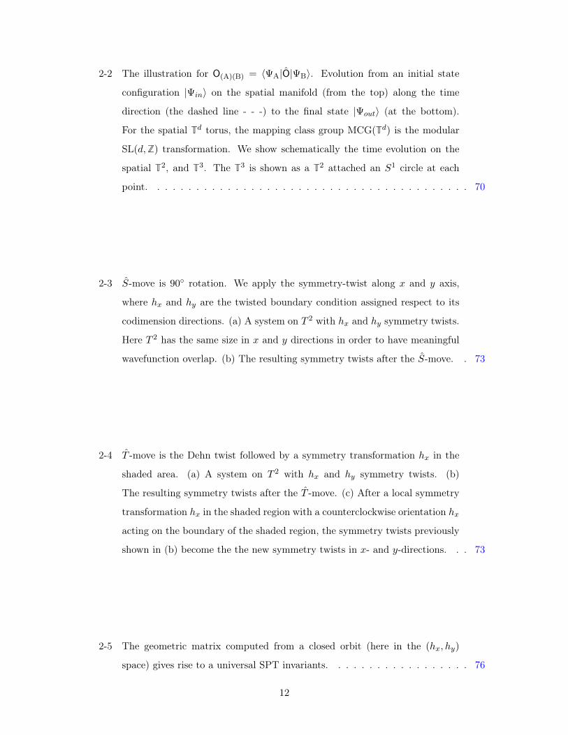
2-2 The illustration for O(A)(B) = ⟨ΨA|O|ΨB⟩. Evolution from an initial state
configuration |Ψ𝑖𝑛⟩ on the spatial manifold (from the top) along the time
direction (the dashed line - - -) to the final state |Ψ𝑜𝑢𝑡⟩ (at the bottom).
For the spatial T𝑑 torus, the mapping class group MCG(T𝑑) is the modular
SL(𝑑,Z) transformation. We show schematically the time evolution on the
spatial T2, and T3. The T3 is shown as a T2 attached an 𝑆1 circle at each
point. . . . . . . . . . . . . . . . . . . . . . . . . . . . . . . . . . . . . . . . . 70
2-3 𝑆-move is 90∘ rotation. We apply the symmetry-twist along 𝑥 and 𝑦 axis,
where ℎ𝑥 and ℎ𝑦 are the twisted boundary condition assigned respect to its
codimension directions. (a) A system on 𝑇 2 with ℎ𝑥 and ℎ𝑦 symmetry twists.
Here 𝑇 2 has the same size in 𝑥 and 𝑦 directions in order to have meaningful
wavefunction overlap. (b) The resulting symmetry twists after the 𝑆-move. . 73
2-4 𝑇 -move is the Dehn twist followed by a symmetry transformation ℎ𝑥 in the
shaded area. (a) A system on 𝑇 2 with ℎ𝑥 and ℎ𝑦 symmetry twists. (b)
The resulting symmetry twists after the 𝑇 -move. (c) After a local symmetry
transformation ℎ𝑥 in the shaded region with a counterclockwise orientation ℎ𝑥
acting on the boundary of the shaded region, the symmetry twists previously
shown in (b) become the the new symmetry twists in 𝑥- and 𝑦-directions. . . 73
2-5 The geometric matrix computed from a closed orbit (here in the (ℎ𝑥, ℎ𝑦)
space) gives rise to a universal SPT invariants. . . . . . . . . . . . . . . . . . 76
12
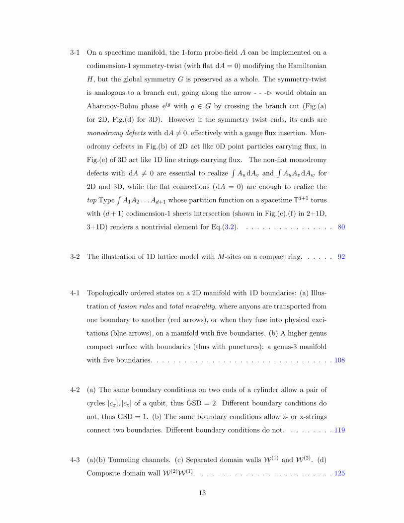
3-1 On a spacetime manifold, the 1-form probe-field 𝐴 can be implemented on a
codimension-1 symmetry-twist (with flat d𝐴 = 0) modifying the Hamiltonian
𝐻, but the global symmetry 𝐺 is preserved as a whole. The symmetry-twist
is analogous to a branch cut, going along the arrow - - -B would obtain an
Aharonov-Bohm phase e𝑖𝑔 with 𝑔 ∈ 𝐺 by crossing the branch cut (Fig.(a)
for 2D, Fig.(d) for 3D). However if the symmetry twist ends, its ends are
monodromy defects with d𝐴 = 0, effectively with a gauge flux insertion. Mon-
odromy defects in Fig.(b) of 2D act like 0D point particles carrying flux, in
Fig.(e) of 3D act like 1D line strings carrying flux. The non-flat monodromy
defects with d𝐴 = 0 are essential to realize∫𝐴𝑢d𝐴𝑣 and
∫𝐴𝑢𝐴𝑣d𝐴𝑤 for
2D and 3D, while the flat connections (d𝐴 = 0) are enough to realize the
top Type∫𝐴1𝐴2 . . . 𝐴𝑑+1 whose partition function on a spacetime T𝑑+1 torus
with (𝑑+1) codimension-1 sheets intersection (shown in Fig.(c),(f) in 2+1D,
3+1D) renders a nontrivial element for Eq.(3.2). . . . . . . . . . . . . . . . . 80
3-2 The illustration of 1D lattice model with 𝑀 -sites on a compact ring. . . . . . 92
4-1 Topologically ordered states on a 2D manifold with 1D boundaries: (a) Illus-
tration of fusion rules and total neutrality, where anyons are transported from
one boundary to another (red arrows), or when they fuse into physical exci-
tations (blue arrows), on a manifold with five boundaries. (b) A higher genus
compact surface with boundaries (thus with punctures): a genus-3 manifold
with five boundaries. . . . . . . . . . . . . . . . . . . . . . . . . . . . . . . . . 108
4-2 (a) The same boundary conditions on two ends of a cylinder allow a pair of
cycles [𝑐𝑥], [𝑐𝑧] of a qubit, thus GSD = 2. Different boundary conditions do
not, thus GSD = 1. (b) The same boundary conditions allow z- or x-strings
connect two boundaries. Different boundary conditions do not. . . . . . . . . 119
4-3 (a)(b) Tunneling channels. (c) Separated domain walls 𝒲(1) and 𝒲(2). (d)
Composite domain wall 𝒲(2)𝒲(1). . . . . . . . . . . . . . . . . . . . . . . . . 125
13
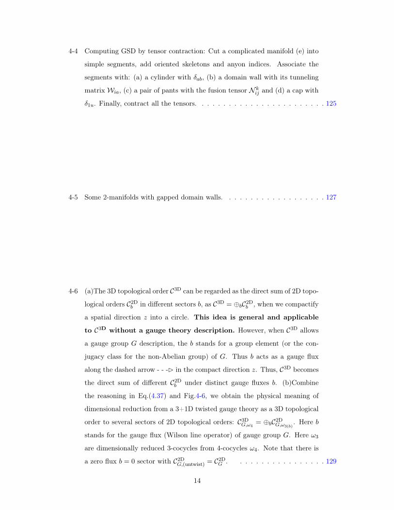
4-4 Computing GSD by tensor contraction: Cut a complicated manifold (e) into
simple segments, add oriented skeletons and anyon indices. Associate the
segments with: (a) a cylinder with 𝛿𝑎𝑏, (b) a domain wall with its tunneling
matrix 𝒲𝑖𝑎, (c) a pair of pants with the fusion tensor 𝒩 𝑘𝑖𝑗 and (d) a cap with
𝛿1𝑢. Finally, contract all the tensors. . . . . . . . . . . . . . . . . . . . . . . . 125
4-5 Some 2-manifolds with gapped domain walls. . . . . . . . . . . . . . . . . . . 127
4-6 (a)The 3D topological order 𝒞3D can be regarded as the direct sum of 2D topo-
logical orders 𝒞2D𝑏 in different sectors 𝑏, as 𝒞3D = ⊕𝑏𝒞2D𝑏 , when we compactify
a spatial direction 𝑧 into a circle. This idea is general and applicable
to 𝒞3D without a gauge theory description. However, when 𝒞3D allows
a gauge group 𝐺 description, the 𝑏 stands for a group element (or the con-
jugacy class for the non-Abelian group) of 𝐺. Thus 𝑏 acts as a gauge flux
along the dashed arrow - - -B in the compact direction 𝑧. Thus, 𝒞3D becomes
the direct sum of different 𝒞2D𝑏 under distinct gauge fluxes 𝑏. (b)Combine
the reasoning in Eq.(4.37) and Fig.4-6, we obtain the physical meaning of
dimensional reduction from a 3+1D twisted gauge theory as a 3D topological
order to several sectors of 2D topological orders: 𝒞3D𝐺,𝜔4= ⊕𝑏𝒞2D𝐺,𝜔3(𝑏)
. Here 𝑏
stands for the gauge flux (Wilson line operator) of gauge group 𝐺. Here 𝜔3
are dimensionally reduced 3-cocycles from 4-cocycles 𝜔4. Note that there is
a zero flux 𝑏 = 0 sector with 𝒞2D𝐺,(untwist) = 𝒞2D𝐺 . . . . . . . . . . . . . . . . . 129
14
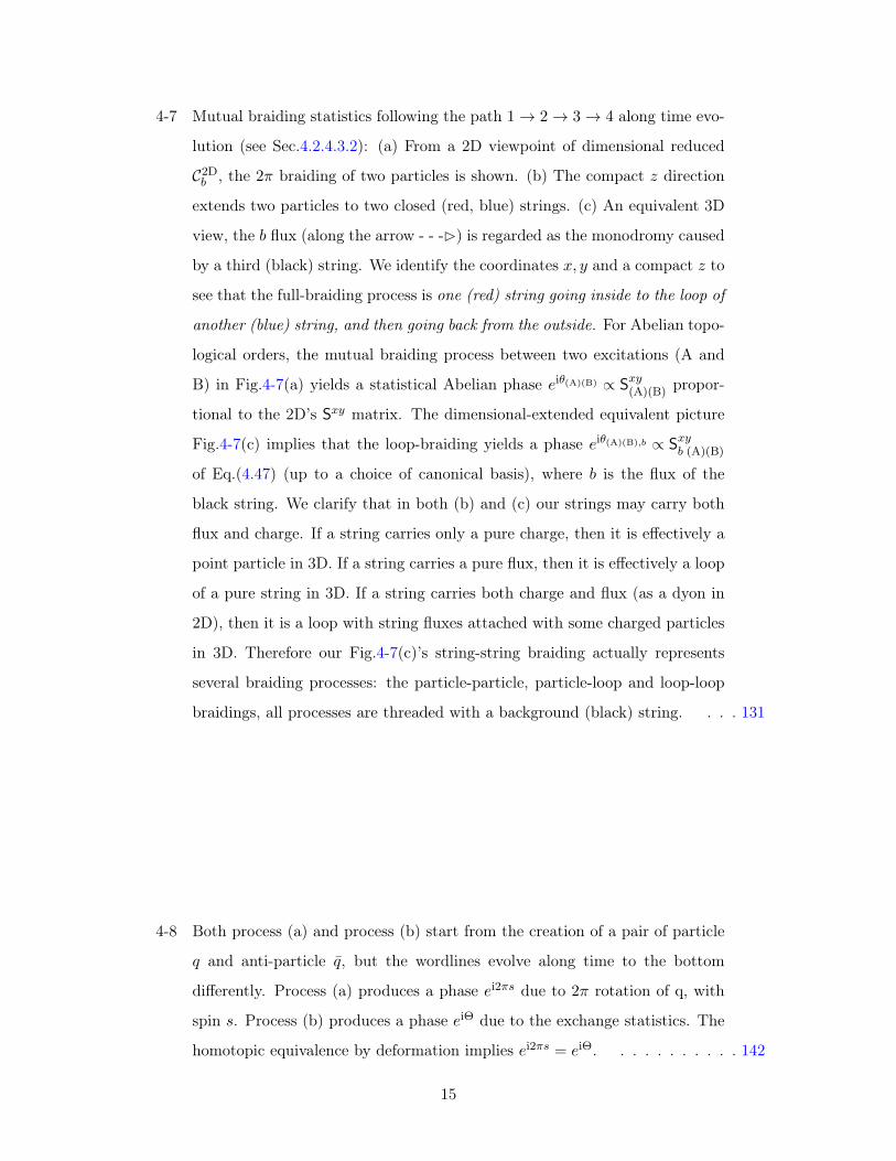
4-7 Mutual braiding statistics following the path 1→ 2→ 3→ 4 along time evo-
lution (see Sec.4.2.4.3.2): (a) From a 2D viewpoint of dimensional reduced
𝒞2D𝑏 , the 2𝜋 braiding of two particles is shown. (b) The compact 𝑧 direction
extends two particles to two closed (red, blue) strings. (c) An equivalent 3D
view, the 𝑏 flux (along the arrow - - -B) is regarded as the monodromy caused
by a third (black) string. We identify the coordinates 𝑥, 𝑦 and a compact 𝑧 to
see that the full-braiding process is one (red) string going inside to the loop of
another (blue) string, and then going back from the outside. For Abelian topo-
logical orders, the mutual braiding process between two excitations (A and
B) in Fig.4-7(a) yields a statistical Abelian phase 𝑒i𝜃(A)(B) ∝ S𝑥𝑦(A)(B) propor-
tional to the 2D’s S𝑥𝑦 matrix. The dimensional-extended equivalent picture
Fig.4-7(c) implies that the loop-braiding yields a phase 𝑒i𝜃(A)(B),𝑏 ∝ S𝑥𝑦𝑏 (A)(B)
of Eq.(4.47) (up to a choice of canonical basis), where 𝑏 is the flux of the
black string. We clarify that in both (b) and (c) our strings may carry both
flux and charge. If a string carries only a pure charge, then it is effectively a
point particle in 3D. If a string carries a pure flux, then it is effectively a loop
of a pure string in 3D. If a string carries both charge and flux (as a dyon in
2D), then it is a loop with string fluxes attached with some charged particles
in 3D. Therefore our Fig.4-7(c)’s string-string braiding actually represents
several braiding processes: the particle-particle, particle-loop and loop-loop
braidings, all processes are threaded with a background (black) string. . . . 131
4-8 Both process (a) and process (b) start from the creation of a pair of particle
𝑞 and anti-particle 𝑞, but the wordlines evolve along time to the bottom
differently. Process (a) produces a phase 𝑒i2𝜋𝑠 due to 2𝜋 rotation of q, with
spin 𝑠. Process (b) produces a phase 𝑒iΘ due to the exchange statistics. The
homotopic equivalence by deformation implies 𝑒i2𝜋𝑠 = 𝑒iΘ. . . . . . . . . . . 142
15
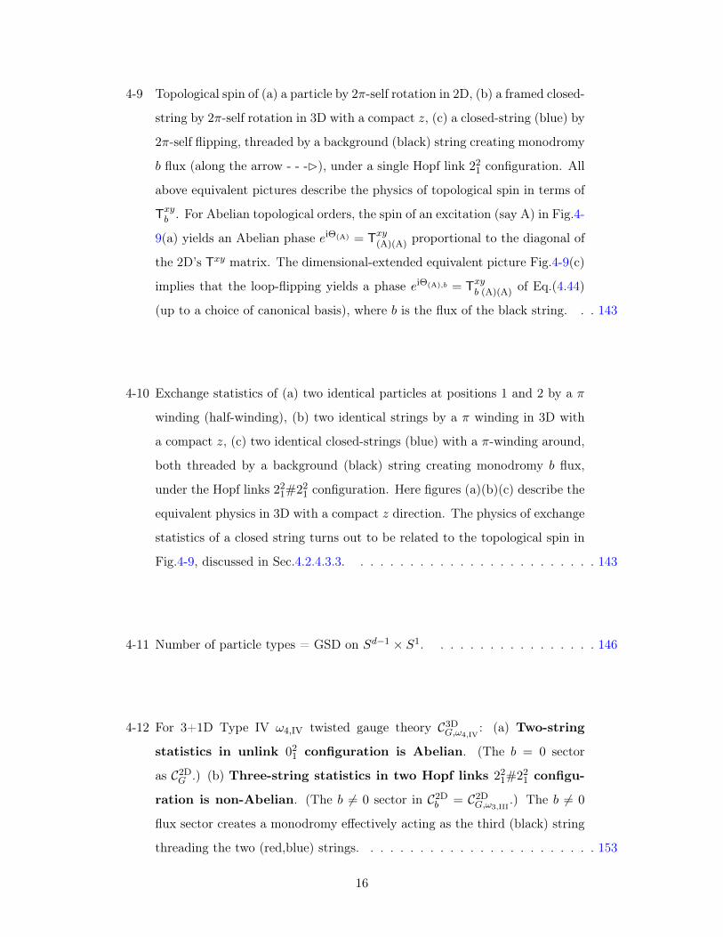
4-9 Topological spin of (a) a particle by 2𝜋-self rotation in 2D, (b) a framed closed-
string by 2𝜋-self rotation in 3D with a compact 𝑧, (c) a closed-string (blue) by
2𝜋-self flipping, threaded by a background (black) string creating monodromy
𝑏 flux (along the arrow - - -B), under a single Hopf link 221 configuration. All
above equivalent pictures describe the physics of topological spin in terms of
T𝑥𝑦𝑏 . For Abelian topological orders, the spin of an excitation (say A) in Fig.4-
9(a) yields an Abelian phase 𝑒iΘ(A) = T𝑥𝑦(A)(A) proportional to the diagonal of
the 2D’s T𝑥𝑦 matrix. The dimensional-extended equivalent picture Fig.4-9(c)
implies that the loop-flipping yields a phase 𝑒iΘ(A),𝑏 = T𝑥𝑦𝑏 (A)(A) of Eq.(4.44)
(up to a choice of canonical basis), where 𝑏 is the flux of the black string. . . 143
4-10 Exchange statistics of (a) two identical particles at positions 1 and 2 by a 𝜋
winding (half-winding), (b) two identical strings by a 𝜋 winding in 3D with
a compact 𝑧, (c) two identical closed-strings (blue) with a 𝜋-winding around,
both threaded by a background (black) string creating monodromy 𝑏 flux,
under the Hopf links 221#221 configuration. Here figures (a)(b)(c) describe the
equivalent physics in 3D with a compact 𝑧 direction. The physics of exchange
statistics of a closed string turns out to be related to the topological spin in
Fig.4-9, discussed in Sec.4.2.4.3.3. . . . . . . . . . . . . . . . . . . . . . . . . 143
4-11 Number of particle types = GSD on 𝑆𝑑−1 × 𝑆1. . . . . . . . . . . . . . . . . 146
4-12 For 3+1D Type IV 𝜔4,IV twisted gauge theory 𝒞3D𝐺,𝜔4,IV: (a) Two-string
statistics in unlink 021 configuration is Abelian. (The 𝑏 = 0 sector
as 𝒞2D𝐺 .) (b) Three-string statistics in two Hopf links 221#221 configu-
ration is non-Abelian. (The 𝑏 = 0 sector in 𝒞2D𝑏 = 𝒞2D𝐺,𝜔3,III.) The 𝑏 = 0
flux sector creates a monodromy effectively acting as the third (black) string
threading the two (red,blue) strings. . . . . . . . . . . . . . . . . . . . . . . . 153
16
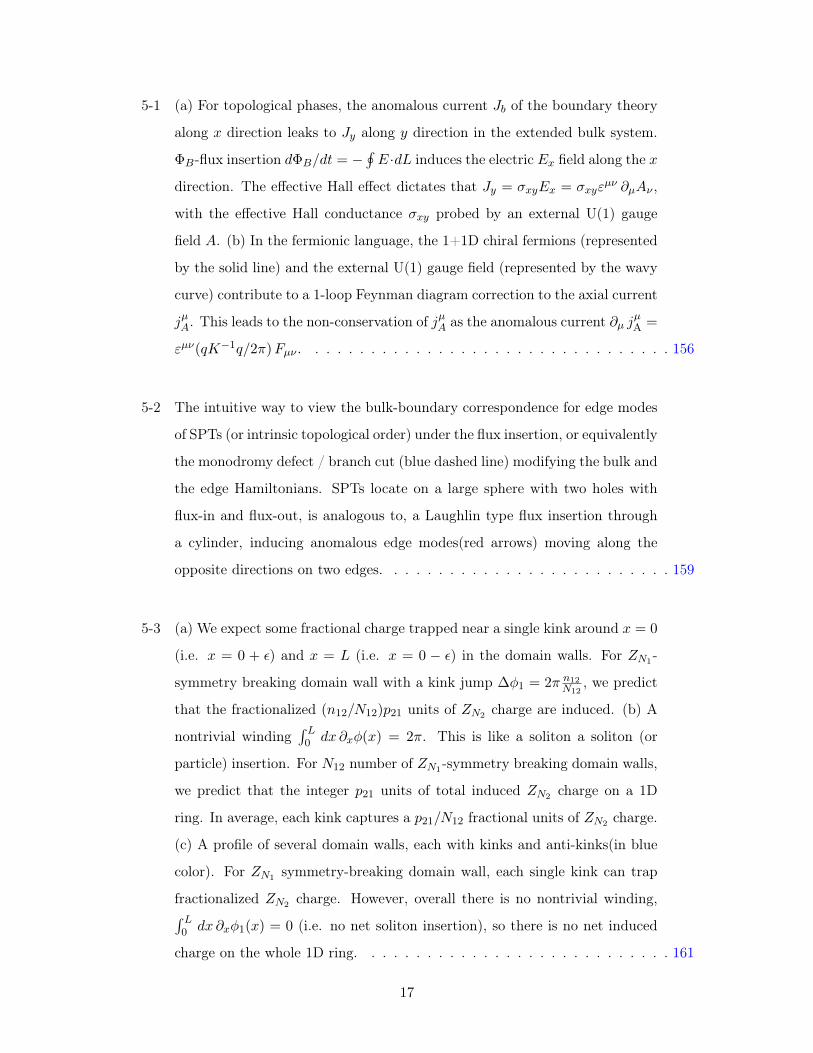
5-1 (a) For topological phases, the anomalous current 𝐽𝑏 of the boundary theory
along 𝑥 direction leaks to 𝐽𝑦 along 𝑦 direction in the extended bulk system.
Φ𝐵-flux insertion 𝑑Φ𝐵/𝑑𝑡 = −∮𝐸 ·𝑑𝐿 induces the electric 𝐸𝑥 field along the 𝑥
direction. The effective Hall effect dictates that 𝐽𝑦 = 𝜎𝑥𝑦𝐸𝑥 = 𝜎𝑥𝑦𝜀𝜇𝜈 𝜕𝜇𝐴𝜈 ,
with the effective Hall conductance 𝜎𝑥𝑦 probed by an external U(1) gauge
field 𝐴. (b) In the fermionic language, the 1+1D chiral fermions (represented
by the solid line) and the external U(1) gauge field (represented by the wavy
curve) contribute to a 1-loop Feynman diagram correction to the axial current
𝑗𝜇𝐴. This leads to the non-conservation of 𝑗𝜇𝐴 as the anomalous current 𝜕𝜇 𝑗𝜇A =
𝜀𝜇𝜈(𝑞𝐾−1𝑞/2𝜋)𝐹𝜇𝜈 . . . . . . . . . . . . . . . . . . . . . . . . . . . . . . . . . 156
5-2 The intuitive way to view the bulk-boundary correspondence for edge modes
of SPTs (or intrinsic topological order) under the flux insertion, or equivalently
the monodromy defect / branch cut (blue dashed line) modifying the bulk and
the edge Hamiltonians. SPTs locate on a large sphere with two holes with
flux-in and flux-out, is analogous to, a Laughlin type flux insertion through
a cylinder, inducing anomalous edge modes(red arrows) moving along the
opposite directions on two edges. . . . . . . . . . . . . . . . . . . . . . . . . . 159
5-3 (a) We expect some fractional charge trapped near a single kink around 𝑥 = 0
(i.e. 𝑥 = 0 + 𝜖) and 𝑥 = 𝐿 (i.e. 𝑥 = 0 − 𝜖) in the domain walls. For 𝑍𝑁1-
symmetry breaking domain wall with a kink jump Δ𝜑1 = 2𝜋 𝑛12𝑁12
, we predict
that the fractionalized (𝑛12/𝑁12)𝑝21 units of 𝑍𝑁2 charge are induced. (b) A
nontrivial winding∫ 𝐿0 𝑑𝑥 𝜕𝑥𝜑(𝑥) = 2𝜋. This is like a soliton a soliton (or
particle) insertion. For 𝑁12 number of 𝑍𝑁1-symmetry breaking domain walls,
we predict that the integer 𝑝21 units of total induced 𝑍𝑁2 charge on a 1D
ring. In average, each kink captures a 𝑝21/𝑁12 fractional units of 𝑍𝑁2 charge.
(c) A profile of several domain walls, each with kinks and anti-kinks(in blue
color). For 𝑍𝑁1 symmetry-breaking domain wall, each single kink can trap
fractionalized 𝑍𝑁2 charge. However, overall there is no nontrivial winding,∫ 𝐿0 𝑑𝑥 𝜕𝑥𝜑1(𝑥) = 0 (i.e. no net soliton insertion), so there is no net induced
charge on the whole 1D ring. . . . . . . . . . . . . . . . . . . . . . . . . . . . 161
17

5-4 In the fermionized language, one can capture the anomaly effect on induced
(fractional) charge/current under soliton background by the 1-loop diagram.[64]
With the solid line — represents fermions, the wavy line :: represents the
external (gauge) field coupling to the induced current 𝐽𝜇 (or charge 𝐽0), and
the dashed line - - represents the scalar soliton (domain walls) background.
Here in Sec.5.2.1.2, instead of fermionizing the theory, we directly address in
the bosonized language to capture the bosonic anomaly. . . . . . . . . . . . . 163
5-5 (a) The induced 2-cocycle from a 2+1D 𝑀3 = 𝑀2 × 𝐼1 topology with a
symmetry-preserving 𝑍𝑁𝑢 flux 𝐴 insertion (b) Here 𝑀2 = 𝑆1 × 𝐼1 is a 2D
spatial cylinder, composed by 𝐴 and 𝐵, with another extra time dimension
𝐼1. Along the 𝐵-line we insert a monodromy defect of 𝑍𝑁1 , such that 𝐴 has
a nontrivial group element value 𝐴 = 𝑔1′𝑔−11 = 𝑔2′𝑔
−12 = 𝑔3′𝑔
−13 ∈ 𝑍𝑁1 . The
induced 2-cocycle 𝛽𝐴(𝐵,𝐶) is a nontrivial element in ℋ2(𝑍𝑁𝑣 × 𝑍𝑁𝑤 ,U(1))
= Z𝑁𝑣𝑤 (here 𝑢, 𝑣, 𝑤 cyclic as 𝜖𝑢𝑣𝑤 = 1), thus which carries a projective
representation. (c) A monodromy defect can viewed as a branch cut induced
by a Φ𝐵 flux insertion (both modifying the Hamiltonians). (d) This means
that when we do dimensional reduction on the compact ring 𝑆1 and view the
reduced system as a 1D line segment, there are 𝑁123 degenerate zero energy
modes (due to the nontrivial projective representation). . . . . . . . . . . . . 168
5-6 The triangulation of a 𝑀3 =𝑀2× 𝐼1 topology (here 𝑀2 is a spatial cylinder
composed by the 𝐴 and 𝐵 direction, with a 𝐼1 time) into three tetrahedra
with branched structures. . . . . . . . . . . . . . . . . . . . . . . . . . . . . . 170
5-7 The 𝑍𝑁1 symmetry breaking domain wall along the red × mark and/or
orange + mark, which induces 𝑁123-fold degenerate zero energy modes. The
situation is very similar to Fig.5-5 (however, there was 𝑍𝑁1 symmetry-
preserving flux insertion). We show that both cases the induced 2-cochain
from calculating path integral ZSPT renders a nontrivial 2-cocycle ofℋ2(𝑍𝑁2×
𝑍𝑁3 ,U(1)) = Z𝑁23 , thus carrying nontrivial projective representation of sym-
metry. . . . . . . . . . . . . . . . . . . . . . . . . . . . . . . . . . . . . . . . . 172
18
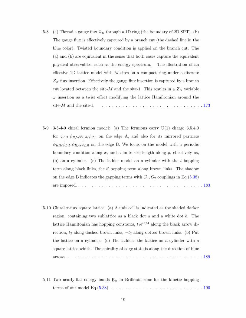
5-8 (a) Thread a gauge flux Φ𝐵 through a 1D ring (the boundary of 2D SPT). (b)
The gauge flux is effectively captured by a branch cut (the dashed line in the
blue color). Twisted boundary condition is applied on the branch cut. The
(a) and (b) are equivalent in the sense that both cases capture the equivalent
physical observables, such as the energy spectrum. The illustration of an
effective 1D lattice model with 𝑀 -sites on a compact ring under a discrete
𝑍𝑁 flux insertion. Effectively the gauge flux insertion is captured by a branch
cut located between the site-𝑀 and the site-1. This results in a 𝑍𝑁 variable
𝜔 insertion as a twist effect modifying the lattice Hamiltonian around the
site-𝑀 and the site-1. . . . . . . . . . . . . . . . . . . . . . . . . . . . . . . 173
5-9 3-5-4-0 chiral fermion model: (a) The fermions carry U(1) charge 3,5,4,0
for 𝜓𝐿,3,𝜓𝑅,5,𝜓𝐿,4,𝜓𝑅,0 on the edge A, and also for its mirrored partners
𝜓𝑅,3,𝜓𝐿,5,𝜓𝑅,4,𝜓𝐿,0 on the edge B. We focus on the model with a periodic
boundary condition along 𝑥, and a finite-size length along 𝑦, effectively as,
(b) on a cylinder. (c) The ladder model on a cylinder with the 𝑡 hopping
term along black links, the 𝑡′ hopping term along brown links. The shadow
on the edge B indicates the gapping terms with 𝐺1, 𝐺2 couplings in Eq.(5.38)
are imposed. . . . . . . . . . . . . . . . . . . . . . . . . . . . . . . . . . . . . . 183
5-10 Chiral 𝜋-flux square lattice: (a) A unit cell is indicated as the shaded darker
region, containing two sublattice as a black dot 𝑎 and a white dot 𝑏. The
lattice Hamiltonian has hopping constants, 𝑡1𝑒𝑖𝜋/4 along the black arrow di-
rection, 𝑡2 along dashed brown links, −𝑡2 along dotted brown links. (b) Put
the lattice on a cylinder. (c) The ladder: the lattice on a cylinder with a
square lattice width. The chirality of edge state is along the direction of blue
arrows. . . . . . . . . . . . . . . . . . . . . . . . . . . . . . . . . . . . . . . . . 189
5-11 Two nearly-flat energy bands E± in Brillouin zone for the kinetic hopping
terms of our model Eq.(5.38). . . . . . . . . . . . . . . . . . . . . . . . . . . . 190
19
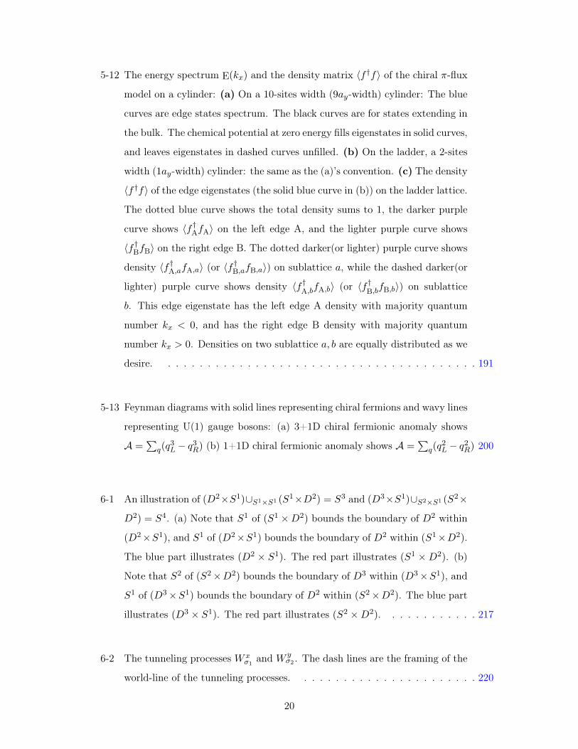
5-12 The energy spectrum E(𝑘𝑥) and the density matrix ⟨𝑓 †𝑓⟩ of the chiral 𝜋-flux
model on a cylinder: (a) On a 10-sites width (9𝑎𝑦-width) cylinder: The blue
curves are edge states spectrum. The black curves are for states extending in
the bulk. The chemical potential at zero energy fills eigenstates in solid curves,
and leaves eigenstates in dashed curves unfilled. (b) On the ladder, a 2-sites
width (1𝑎𝑦-width) cylinder: the same as the (a)’s convention. (c) The density
⟨𝑓 †𝑓⟩ of the edge eigenstates (the solid blue curve in (b)) on the ladder lattice.
The dotted blue curve shows the total density sums to 1, the darker purple
curve shows ⟨𝑓 †A𝑓A⟩ on the left edge A, and the lighter purple curve shows
⟨𝑓 †B𝑓B⟩ on the right edge B. The dotted darker(or lighter) purple curve shows
density ⟨𝑓 †A,𝑎𝑓A,𝑎⟩ (or ⟨𝑓 †B,𝑎𝑓B,𝑎⟩) on sublattice 𝑎, while the dashed darker(or
lighter) purple curve shows density ⟨𝑓 †A,𝑏𝑓A,𝑏⟩ (or ⟨𝑓 †
B,𝑏𝑓B,𝑏⟩) on sublattice
𝑏. This edge eigenstate has the left edge A density with majority quantum
number 𝑘𝑥 < 0, and has the right edge B density with majority quantum
number 𝑘𝑥 > 0. Densities on two sublattice 𝑎, 𝑏 are equally distributed as we
desire. . . . . . . . . . . . . . . . . . . . . . . . . . . . . . . . . . . . . . . . 191
5-13 Feynman diagrams with solid lines representing chiral fermions and wavy lines
representing U(1) gauge bosons: (a) 3+1D chiral fermionic anomaly shows
𝒜 =∑
𝑞(𝑞3𝐿 − 𝑞3𝑅) (b) 1+1D chiral fermionic anomaly shows 𝒜 =
∑𝑞(𝑞
2𝐿 − 𝑞2𝑅) 200
6-1 An illustration of (𝐷2×𝑆1)∪𝑆1×𝑆1 (𝑆1×𝐷2) = 𝑆3 and (𝐷3×𝑆1)∪𝑆2×𝑆1 (𝑆2×
𝐷2) = 𝑆4. (a) Note that 𝑆1 of (𝑆1 ×𝐷2) bounds the boundary of 𝐷2 within
(𝐷2×𝑆1), and 𝑆1 of (𝐷2×𝑆1) bounds the boundary of 𝐷2 within (𝑆1×𝐷2).
The blue part illustrates (𝐷2 × 𝑆1). The red part illustrates (𝑆1 ×𝐷2). (b)
Note that 𝑆2 of (𝑆2×𝐷2) bounds the boundary of 𝐷3 within (𝐷3×𝑆1), and
𝑆1 of (𝐷3×𝑆1) bounds the boundary of 𝐷2 within (𝑆2×𝐷2). The blue part
illustrates (𝐷3 × 𝑆1). The red part illustrates (𝑆2 ×𝐷2). . . . . . . . . . . . 217
6-2 The tunneling processes 𝑊 𝑥𝜎1 and 𝑊 𝑦
𝜎2 . The dash lines are the framing of the
world-line of the tunneling processes. . . . . . . . . . . . . . . . . . . . . . . 220
20
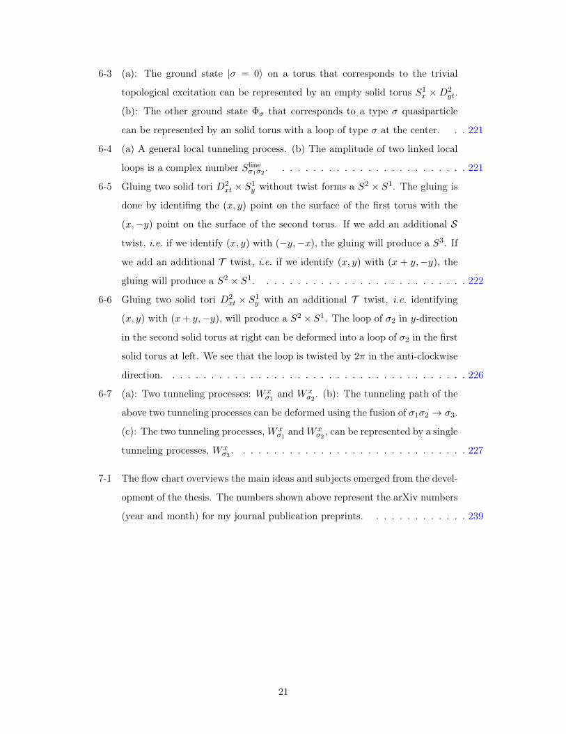
6-3 (a): The ground state |𝜎 = 0⟩ on a torus that corresponds to the trivial
topological excitation can be represented by an empty solid torus 𝑆1𝑥 ×𝐷2
𝑦𝑡.
(b): The other ground state Φ𝜎 that corresponds to a type 𝜎 quasiparticle
can be represented by an solid torus with a loop of type 𝜎 at the center. . . 221
6-4 (a) A general local tunneling process. (b) The amplitude of two linked local
loops is a complex number 𝑆line𝜎1��2 . . . . . . . . . . . . . . . . . . . . . . . . . 221
6-5 Gluing two solid tori 𝐷2𝑥𝑡 × 𝑆1
𝑦 without twist forms a 𝑆2 × 𝑆1. The gluing is
done by identifing the (𝑥, 𝑦) point on the surface of the first torus with the
(𝑥,−𝑦) point on the surface of the second torus. If we add an additional 𝒮
twist, i.e. if we identify (𝑥, 𝑦) with (−𝑦,−𝑥), the gluing will produce a 𝑆3. If
we add an additional 𝒯 twist, i.e. if we identify (𝑥, 𝑦) with (𝑥 + 𝑦,−𝑦), the
gluing will produce a 𝑆2 × 𝑆1. . . . . . . . . . . . . . . . . . . . . . . . . . . 222
6-6 Gluing two solid tori 𝐷2𝑥𝑡 × 𝑆1
𝑦 with an additional 𝒯 twist, i.e. identifying
(𝑥, 𝑦) with (𝑥+ 𝑦,−𝑦), will produce a 𝑆2 × 𝑆1. The loop of 𝜎2 in 𝑦-direction
in the second solid torus at right can be deformed into a loop of 𝜎2 in the first
solid torus at left. We see that the loop is twisted by 2𝜋 in the anti-clockwise
direction. . . . . . . . . . . . . . . . . . . . . . . . . . . . . . . . . . . . . . . 226
6-7 (a): Two tunneling processes: 𝑊 𝑥𝜎1 and 𝑊 𝑥
𝜎2 . (b): The tunneling path of the
above two tunneling processes can be deformed using the fusion of 𝜎1𝜎2 → 𝜎3.
(c): The two tunneling processes, 𝑊 𝑥𝜎1 and𝑊 𝑥
𝜎2 , can be represented by a single
tunneling processes, 𝑊 𝑥𝜎3 . . . . . . . . . . . . . . . . . . . . . . . . . . . . . . 227
7-1 The flow chart overviews the main ideas and subjects emerged from the devel-
opment of the thesis. The numbers shown above represent the arXiv numbers
(year and month) for my journal publication preprints. . . . . . . . . . . . . 239
21

22

List of Tables
1.1 Some properties of SPTs and TOs. . . . . . . . . . . . . . . . . . . . . . . . . 30
1.2 Theory and experiment progress for TOs and SPTs in a simplified timeline.
Here topological insulator in 2D means the Quantum Spin Hall effect (QSH).
Here “exp.” abbreviates the experiment and “theo.” abbreviates the theory. . 35
1.3 Perspective on topological states in terms of symmetry, topology and anomalies. 41
1.4 The interplay of classical, quantum and spacetime topology. . . . . . . . . . . 41
3.1 Some derived results on the correspondence between the spacetime parti-
tion function of probe fields (the second column) and the cocycles of
the cohomology group (the third column) for any finite Abelian group
𝐺 =∏𝑢 𝑍𝑁𝑢 . The first column provides the spacetime dimension: (𝑑+ 1)D.
The even/odd effect means that whether their corresponding cocycles are
nontrivial or trivial(as coboundary) depends on the level 𝑝 and 𝑁 (of the
symmetry group 𝑍𝑁 ) is even/odd. Details are explained in Sec 3.1.4. . . . . 86
3.2 From partition functions of fields to Künneth formula. Here we con-
sider a finite Abelian group 𝐺 =∏𝑢 𝑍𝑁𝑢 . The field theory result can map to
the derived facts about the cohomology group and its cocycles. The first col-
umn provides the spacetime dimension: (𝑑+1)D. Here the level-quantization
is shown in a shorthand way with only 𝑝.. written, the explicit coefficients can
be found. In some row, we abbreviate ℋ1(Z𝑛𝑗 ,R/Z) ≡ ℋ1(Z𝑛𝑗 ). The torsion
product TorZ1 ≡ �Z evokes a wedge product ∧ structure in the corresponding
field theory, while the tensor product ⊗Z evokes appending an extra exterior
derivative ∧d structure in the corresponding field theory. This simple obser-
vation maps the field theoretic path integral to its correspondence in Künneth
formula. . . . . . . . . . . . . . . . . . . . . . . . . . . . . . . . . . . . . . . 87
23
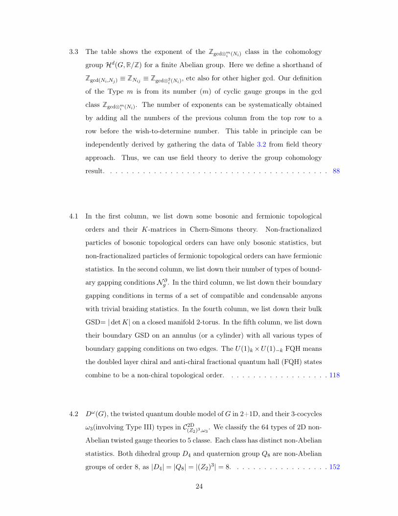
3.3 The table shows the exponent of the Zgcd⊗𝑚𝑖 (𝑁𝑖) class in the cohomology
group ℋ𝑑(𝐺,R/Z) for a finite Abelian group. Here we define a shorthand of
Zgcd(𝑁𝑖,𝑁𝑗) ≡ Z𝑁𝑖𝑗 ≡ Zgcd⊗2𝑖 (𝑁𝑖)
, etc also for other higher gcd. Our definition
of the Type 𝑚 is from its number (𝑚) of cyclic gauge groups in the gcd
class Zgcd⊗𝑚𝑖 (𝑁𝑖). The number of exponents can be systematically obtained
by adding all the numbers of the previous column from the top row to a
row before the wish-to-determine number. This table in principle can be
independently derived by gathering the data of Table 3.2 from field theory
approach. Thus, we can use field theory to derive the group cohomology
result. . . . . . . . . . . . . . . . . . . . . . . . . . . . . . . . . . . . . . . . . 88
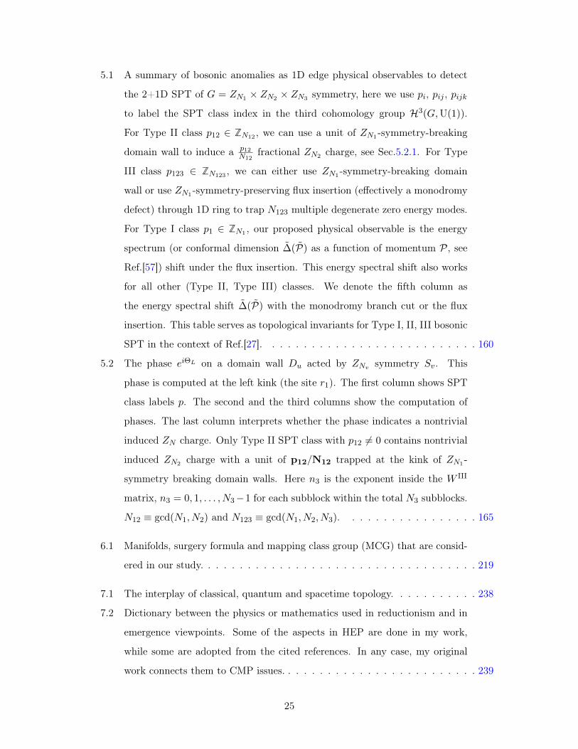
4.1 In the first column, we list down some bosonic and fermionic topological
orders and their 𝐾-matrices in Chern-Simons theory. Non-fractionalized
particles of bosonic topological orders can have only bosonic statistics, but
non-fractionalized particles of fermionic topological orders can have fermionic
statistics. In the second column, we list down their number of types of bound-
ary gapping conditions 𝒩 𝜕𝑔 . In the third column, we list down their boundary
gapping conditions in terms of a set of compatible and condensable anyons
with trivial braiding statistics. In the fourth column, we list down their bulk
GSD= |det𝐾| on a closed manifold 2-torus. In the fifth column, we list down
their boundary GSD on an annulus (or a cylinder) with all various types of
boundary gapping conditions on two edges. The 𝑈(1)𝑘×𝑈(1)−𝑘 FQH means
the doubled layer chiral and anti-chiral fractional quantum hall (FQH) states
combine to be a non-chiral topological order. . . . . . . . . . . . . . . . . . . 118
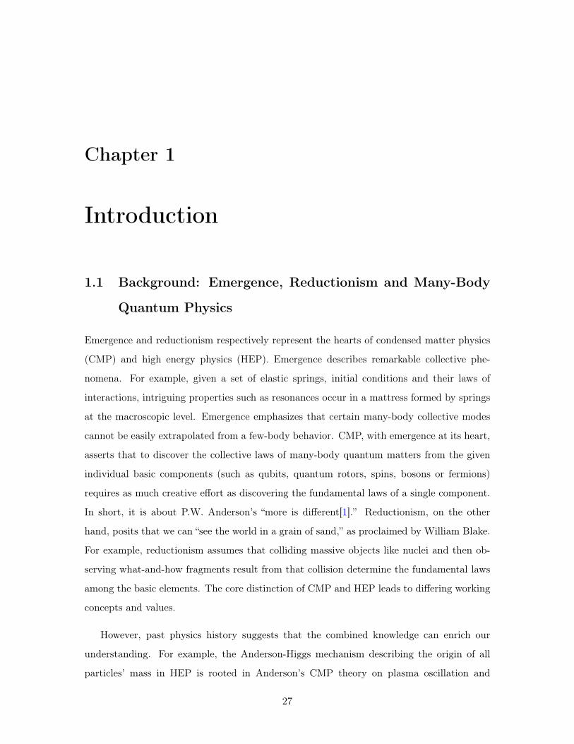
4.2 𝐷𝜔(𝐺), the twisted quantum double model of 𝐺 in 2+1D, and their 3-cocycles
𝜔3(involving Type III) types in 𝒞2D(𝑍2)3,𝜔3. We classify the 64 types of 2D non-
Abelian twisted gauge theories to 5 classe. Each class has distinct non-Abelian
statistics. Both dihedral group 𝐷4 and quaternion group 𝑄8 are non-Abelian
groups of order 8, as |𝐷4| = |𝑄8| = |(𝑍2)3| = 8. . . . . . . . . . . . . . . . . . 152
24
5.1 A summary of bosonic anomalies as 1D edge physical observables to detect
the 2+1D SPT of 𝐺 = 𝑍𝑁1 × 𝑍𝑁2 × 𝑍𝑁3 symmetry, here we use 𝑝𝑖, 𝑝𝑖𝑗 , 𝑝𝑖𝑗𝑘
to label the SPT class index in the third cohomology group ℋ3(𝐺,U(1)).
For Type II class 𝑝12 ∈ Z𝑁12 , we can use a unit of 𝑍𝑁1-symmetry-breaking
domain wall to induce a 𝑝12𝑁12
fractional 𝑍𝑁2 charge, see Sec.5.2.1. For Type
III class 𝑝123 ∈ Z𝑁123 , we can either use 𝑍𝑁1-symmetry-breaking domain
wall or use 𝑍𝑁1-symmetry-preserving flux insertion (effectively a monodromy
defect) through 1D ring to trap 𝑁123 multiple degenerate zero energy modes.
For Type I class 𝑝1 ∈ Z𝑁1 , our proposed physical observable is the energy
spectrum (or conformal dimension Δ(𝒫) as a function of momentum 𝒫, see
Ref.[57]) shift under the flux insertion. This energy spectral shift also works
for all other (Type II, Type III) classes. We denote the fifth column as
the energy spectral shift Δ(𝒫) with the monodromy branch cut or the flux
insertion. This table serves as topological invariants for Type I, II, III bosonic
SPT in the context of Ref.[27]. . . . . . . . . . . . . . . . . . . . . . . . . . . 160
5.2 The phase 𝑒𝑖Θ𝐿 on a domain wall 𝐷𝑢 acted by 𝑍𝑁𝑣 symmetry 𝑆𝑣. This
phase is computed at the left kink (the site 𝑟1). The first column shows SPT
class labels 𝑝. The second and the third columns show the computation of
phases. The last column interprets whether the phase indicates a nontrivial
induced 𝑍𝑁 charge. Only Type II SPT class with 𝑝12 = 0 contains nontrivial
induced 𝑍𝑁2 charge with a unit of p12/N12 trapped at the kink of 𝑍𝑁1-
symmetry breaking domain walls. Here 𝑛3 is the exponent inside the 𝑊 III
matrix, 𝑛3 = 0, 1, . . . , 𝑁3−1 for each subblock within the total 𝑁3 subblocks.
𝑁12 ≡ gcd(𝑁1, 𝑁2) and 𝑁123 ≡ gcd(𝑁1, 𝑁2, 𝑁3). . . . . . . . . . . . . . . . . 165
6.1 Manifolds, surgery formula and mapping class group (MCG) that are consid-
ered in our study. . . . . . . . . . . . . . . . . . . . . . . . . . . . . . . . . . . 219
7.1 The interplay of classical, quantum and spacetime topology. . . . . . . . . . . 238
7.2 Dictionary between the physics or mathematics used in reductionism and in
emergence viewpoints. Some of the aspects in HEP are done in my work,
while some are adopted from the cited references. In any case, my original
work connects them to CMP issues. . . . . . . . . . . . . . . . . . . . . . . . . 239
25

26
Chapter 1
Introduction
1.1 Background: Emergence, Reductionism and Many-Body
Quantum Physics
Emergence and reductionism respectively represent the hearts of condensed matter physics
(CMP) and high energy physics (HEP). Emergence describes remarkable collective phe-
nomena. For example, given a set of elastic springs, initial conditions and their laws of
interactions, intriguing properties such as resonances occur in a mattress formed by springs
at the macroscopic level. Emergence emphasizes that certain many-body collective modes
cannot be easily extrapolated from a few-body behavior. CMP, with emergence at its heart,
asserts that to discover the collective laws of many-body quantum matters from the given
individual basic components (such as qubits, quantum rotors, spins, bosons or fermions)
requires as much creative effort as discovering the fundamental laws of a single component.
In short, it is about P.W. Anderson’s “more is different[1].” Reductionism, on the other
hand, posits that we can “see the world in a grain of sand,” as proclaimed by William Blake.
For example, reductionism assumes that colliding massive objects like nuclei and then ob-
serving what-and-how fragments result from that collision determine the fundamental laws
among the basic elements. The core distinction of CMP and HEP leads to differing working
concepts and values.
However, past physics history suggests that the combined knowledge can enrich our
understanding. For example, the Anderson-Higgs mechanism describing the origin of all
particles’ mass in HEP is rooted in Anderson’s CMP theory on plasma oscillation and
27
superconductivity. The macro-scale inflation theory of the universe of HEP cosmology is
inspired by the micro-scale supercooling phase transition of CMP. There are many more
successful and remarkable examples, such as those examples concerning the interplay of
fractionalization, quantum anomalies and topological non-perturbative aspects of quantum
systems such as quantum Hall states (see [2, 3, 4, 5, 6] for an overview), which we will
gradually explore later. In this thesis, we explore the aspects of symmetry, topology and
anomalies in quantum matter from the intertwining viewpoints of CMP and HEP.
Why do we study quantum matter? Because the quantum matter not only resides in an
outer space (the spacetime we are familiar with at the classical level), but also resides in an
inner but gigantic larger space, the Hilbert space of quantum systems. The Hilbert space ℋ
of a many-body quantum system is enormously huge. For a number of𝑁 spin-12 particles, the
dimension of ℋ grows exponentially as dim(ℋ) = 2𝑁 . Yet we have not taken into account
other degrees of freedom, like orbitals, charges and interactions, etc. So for a merely 1-
mole of atoms with a tiny weight of a few grams, its dimension is dim(ℋ) > 26.02×10²³ !
Hence, studying the structure of Hilbert space may potentially guide us to systematically
explore many mathematical structures both ones we have imagined and ones we have not yet
imagined, and explore the possible old and new emergent principles hidden in all branches
of physics, including CMP, HEP and even astro- or cosmology physics.
In particular, we will take a modest step, focusing on the many-body quantum systems
at zero temperature where there are unique or degenerated bulk ground states well-separated
from energetic excitation with finite energy gaps, while the surfaces of these states exhibit
quantum anomalies. These phases of matter are termed symmetry-protected topological
states (SPTs) and topologically ordered states (TOs).
1.1.1 Landau symmetry-breaking orders, quantum orders, SPTs and topo-
logical orders: Classification and characterization
What are the phases of matter (or the states of matter)? Phases of matter are the collective
behaviors of many-body systems described by some macroscopic scale of parameters. The
important concepts to characterize the “phases” notions are universality, phase transitions,
and fixed points [7]. The universality class means that a large class of systems can exhibit
the same or similar behavior even though their microscopic degrees of freedom can be very
different. By tuning macroscopic scale of parameters such as temperature, doping or pres-
28
sure, the phase can encounter phase transitions. Particularly at the low energy and long
wave length limit, the universal behavior can be controlled by the fixed points of the phase
diagram. Some fixed points sit inside the mid of a phase region, some fixed points are critical
points at the phase transition boundaries. A powerful theory of universality class should
describe the behavior of phases and phase transitions of matter.
Lev Landau established one such a powerful framework in 1930s known as Landau
symmetry-breaking theory [8]. It can describe many phases and phase transitions with
symmetry-breaking orders, including crystal or periodic charge ordering (breaking the con-
tinuous translational symmetry), ferromagnets (breaking the spin rotational symmetry) and
superfluids (breaking the U(1) symmetry of bosonic phase rotation). Landau symmetry-
breaking theory still can be captured by the semi-classical Ginzburg-Landau theory [9, 10].
However, it is now known that there are certain orders at zero temperature beyond
the semi-classical Landau’s symmetry-breaking orders. The new kind of order is referred
as quantum order [11], where the quantum-many body behavior exhibits new phenomena
without the necessity of classical analogy. The full scope of quantum order containing gapless
or gapped excitations is too rich to be properly examined in my thesis. I will focus on the
gapped quantum order: including SPTs [12, 13] and topological orders (TOs) [14, 15]. The
first few examples of TOs are integer quantum Hall states (IQHs) discovered in 1980 [16] and
fractional quantum Hall states (FQHs) in 1982 [17, 18]. Quantum Hall states and TOs are
exotic because they are not distinguished by symmetry-breaking, local order parameters, or
the long-range correlation. These new kinds of orders require a new paradigm going beyond
the old paradigm of Landau’s theory.
Classification and characterization of quantum phases of matter: So what ex-
actly are SPTs and TOs? SPTs and TOs are quantum phases of matter with bulk insulating
gaps while the surfaces are anomalous (such as gapless edge modes) which cannot exist
in its own dimensions. One important strategy to guide us understand or even define the
phases of matter is doing the classification and characterization. By doing classification, we
are counting the number of distinct states (of SPTs and TOs) and giving them a proper
label and a name. For example, giving the spacetime dimension and the symmetry group,
etc; can we determined how many phases there are? By doing characterization, we are list-
ing their properties by physical observables. How can we potentially measure them in the
experiments?
29
Below we organize the key features of SPTs and TOs first, in Table 1.1. There are a
few important concepts for physical measurement we need to introduce: (i) ground state
degeneracy, (ii) entanglement and (topological) entanglement entropy, (iii) fractionalized
charge and fractional statistics.
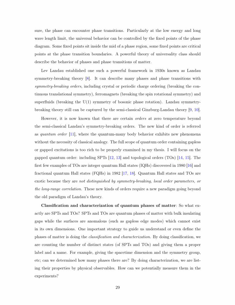
Symmetry-Protected Topological states (SPTs) & Topological Orders (TOs):Short/Long ranged entangled states at zero temperature.↔ Yes/No deformed to trivial product states by local unitary transformations.No/Likely nontrivial topological entanglement entropy.No/Likely bulk fractionalized charge → edge may have fractionalized charges.No/Likely bulk anyonic statistics → edge may have degeneracy.No/Yes (Likely) spatial topology-dependent GSD.No/Yes (Likely) non-Abelian Berry’s phases on coupling const moduli space
Table 1.1: Some properties of SPTs and TOs.
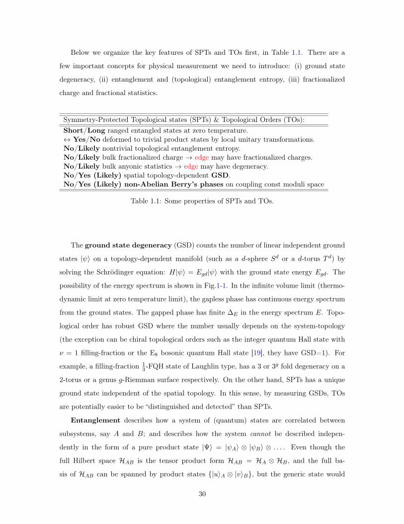
The ground state degeneracy (GSD) counts the number of linear independent ground
states |𝜓⟩ on a topology-dependent manifold (such as a 𝑑-sphere 𝑆𝑑 or a 𝑑-torus 𝑇 𝑑) by
solving the Schrödinger equation: 𝐻|𝜓⟩ = 𝐸𝑔𝑑|𝜓⟩ with the ground state energy 𝐸𝑔𝑑. The
possibility of the energy spectrum is shown in Fig.1-1. In the infinite volume limit (thermo-
dynamic limit at zero temperature limit), the gapless phase has continuous energy spectrum
from the ground states. The gapped phase has finite Δ𝐸 in the energy spectrum 𝐸. Topo-
logical order has robust GSD where the number usually depends on the system-topology
(the exception can be chiral topological orders such as the integer quantum Hall state with
𝜈 = 1 filling-fraction or the E8 bosonic quantum Hall state [19], they have GSD=1). For
example, a filling-fraction 13 -FQH state of Laughlin type, has a 3 or 3𝑔 fold degeneracy on a
2-torus or a genus 𝑔-Riemman surface respectively. On the other hand, SPTs has a unique
ground state independent of the spatial topology. In this sense, by measuring GSDs, TOs
are potentially easier to be “distinguished and detected” than SPTs.
Entanglement describes how a system of (quantum) states are correlated between
subsystems, say 𝐴 and 𝐵; and describes how the system cannot be described indepen-
dently in the form of a pure product state |Ψ⟩ = |𝜓𝐴⟩ ⊗ |𝜓𝐵⟩ ⊗ . . . . Even though the
full Hilbert space ℋ𝐴𝐵 is the tensor product form ℋ𝐴𝐵 = ℋ𝐴 ⊗ ℋ𝐵, and the full ba-
sis of ℋ𝐴𝐵 can be spanned by product states {|𝑢⟩𝐴 ⊗ |𝑣⟩𝐵}, but the generic state would
30
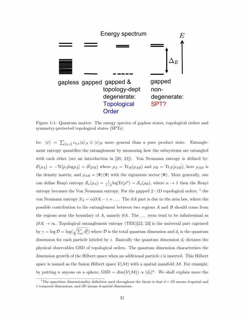
gapless
Energy spectrum
gapped gapped & topology-dept degenerate: Topological Order
gapped non-degenerate: SPT?
Figure 1-1: Quantum matter: The energy spectra of gapless states, topological orders andsymmetry-protected topological states (SPTs).
be: |𝜓⟩ =∑
{𝑢,𝑣} 𝑐𝑢,𝑣|𝑢⟩𝐴 ⊗ |𝑣⟩𝐵 more general than a pure product state. Entangle-
ment entropy quantifies the entanglement by measuring how the subsystems are entangled
with each other (see an introduction in [20, 21]). Von Neumann entropy is defined by:
𝒮(𝜌𝐴) = −Tr[𝜌𝐴log𝜌𝐴] = 𝒮(𝜌𝐵) where 𝜌𝐴 = Tr𝐵(𝜌𝐴𝐵) and 𝜌𝐵 = Tr𝐴(𝜌𝐴𝐵), here 𝜌𝐴𝐵 is
the density matrix, and 𝜌𝐴𝐵 = |Ψ⟩⟨Ψ| with the eigenstate sector |Ψ⟩. More generally, one
can define Renyi entropy 𝒮𝛼(𝜌𝐴) = 11−𝛼 logTr(𝜌𝛼) = 𝒮𝛼(𝜌𝐵), where 𝛼 → 1 then the Renyi
entropy becomes the Von Neumann entropy. For the gapped 2+1D topological orders, 1 the
von Neumann entropy 𝑆𝐴 = 𝛼|𝜕𝐴|−𝛾+ . . . . The 𝜕𝐴 part is due to the area law, where the
possible contribution to the entanglement between two regions 𝐴 and 𝐵 should come from
the regions near the boundary of 𝐴, namely 𝜕𝐴. The . . . term tend to be infinitesimal as
|𝜕𝐴| → ∞. Topological entanglement entropy (TEE)[22, 23] is the universal part captured
by 𝛾 = log𝒟 = log(√∑
𝑖 𝑑2𝑖 ) where 𝒟 is the total quantum dimension and 𝑑𝑖 is the quantum
dimension for each particle labeled by 𝑖. Basically the quantum dimension 𝑑𝑖 dictates the
physical observables GSD of topological orders. The quantum dimension characterizes the
dimension growth of the Hilbert space when an additional particle 𝑖 is inserted. This Hilbert
space is named as the fusion Hilbert space 𝒱(ℳ) with a spatial manifoldℳ. For example,
by putting 𝑛 anyons on a sphere, GSD = dim(𝒱(ℳ)) ∝ (𝑑𝑖)𝑛. We shall explain more the
1The spacetime dimensionality definition used throughout the thesis is that 𝑑+ 1D means 𝑑-spatial and1 temporal dimensions, and 𝑑D means 𝑑-spatial dimensions.
31
meaning of 𝒟 and 𝑑𝑖 later in the chapters.
Fractionalized charge and fractional statistics are introduced in a review of selected
papers in [6], [5]. Due to interactions, the emergent quasi-excitations of the system can
have fractionalized charge and fractional statistics respect to the original unit charge. To
define fractional statistics as a meaningful measurable quantities in many-body systems, it
requires the adiabatic braiding process between quasi-excitations in a gapped phase at zero
temperature. The wavefunction of the whole system will obtain a 𝑒 i𝜃 phase with a fractional
of 2𝜋 value of 𝜃. The excitation with fractional statistics is called anyon.
The first known experimental example exhibits all exotic phenomena of (i) spatial topology-
dependent GSD, (ii) entanglement and TEE, (iii) fractionalized charge and fractional statis-
tics, is the FQHs with 𝜈 = 1/3-filling fraction discovered in 1982 [17, 18]. FQHs is a truly
topologically ordered state. Some of other topological orders and SPTs may not have all
these nontrivial properties. We should summarize them below.
For SPTs:
• Gapped-bulk short ranged entangled states (SREs).
• No topological entanglement entropy.
• No bulk fractionalized charge → edge may carry fractionalized charge
• No bulk anyonic statistics (GSD = 1) → gapped edge may have degeneracy.
• The bulk realizes the symmetry with a global symmetry group 𝐺 onsite (here we
exclude the non-onsite space symmetry such as spatial translation or point group
symmetry, etc; the time reveal symmetry can still be defined as an anti-unitary on-site
symmetry). The symmetry-operator is onsite, if it has the form: 𝑈(𝑔) = ⊗𝑗𝑈𝑗(𝑔), 𝑔 ∈
𝐺. It can be written as the tensor product structure of 𝑈𝑗(𝑔) acting on each site 𝑗.
The boundary realizes the symmetry 𝐺 non-onsite, exhibiting one of the following:
(1) gapless edge modes, or (2) GSD from symmetry breaking gapped boundary, or (3)
GSD from the gapped surface topological order on the boundary.
For intrinsic topological orders:
• Gapped-bulk long ranged entangled states (LREs).
• Robust gapless edge states without the symmetry protection.
32
• (usually) with topological entanglement entropy.
• (usually) Bulk fractionalized charge.
• (usually) Bulk fractionalized statistics.
• (1) Spatial topology-dependent GSD.
• (2) Non-Abelian (Berry) geometric structure on the Hamiltonian’s coupling
constant moduli space.
Some remarks follow: The “usually” quoted above is to exclude some exceptional cases such
as IQHs and E8 QH states. The short ranged entangled (SREs) and long ranged entangled
states (LREs) are distinguished by the local unitary (LU) transformation. SREs can be
deformed to a trivial direct product state in the real space under the LU transformation;
SREs is distinguished from a trivial product state on each site only if there is some symmetry-
protection so that along the path connecting the state to a trivial product state breaks the
symmetry. LREs on the other hand cannot be connected to a trivial product state via
LU transformation even if we remove all the symmetries. Thus the LU transformation is
an important concept which guide us to classify the distinct states in SPTs and TOs by
determining whether two states are connected via LU transformations.
The essences of orders: Apart from the summary on physical comparison of Table 1.1,
we comment that for there are microscopic or field theories, trying to capture the essences of
Landau’s symmetry-breaking order, TOs and SPTs. For example, Landau’s theory and
Bardeen-Cooper-Schrieffer (BCS) theory is powerful for understanding symmetry-
breaking orders, but the essence of symmetry-breaking order is indeed emphasized later
as the long range correlation, symmetry-breaking local order parameters and the long-range
order [see C.N.Yang’s review on the (off-diagonal) long range order[24]]. Then, there are
Laughlin’s theory for FQHs of topological orders, and there are topological quantum field
theory (TQFT) [25, 26] approach of topological phases. But what is the physical essence
of topological orders? After all, Laughlin’s approach focus mainly on the wavefunction,
and TQFT only capture the low energy long-wavelength physics and TQFT may not full
classify or describe topological phases of matter in any dimension. The essence of topological
orders is not the quantized Hall conductance (which will be broken down to non-quantized
if the particle number conservation is broken). The essence of topological orders should
33
not depend on the notion of symmetry. The essence of topological orders is actually the
topological GSD, the non-Abelian geometric phases and the long-range entanglement. For
topological orders, there are degenerate ground states depending on the spatial-topology,
and we can characterize the topological order by adiabatically transporting the ground state
sectors. However, for SPTs, unfortunately we do not have the concept of non-Abelian
geometric phases. How do we capture the essence of SPTs? There are indeed such a tool we
can develop, named symmetry-twist [27, 28, 29]. The essence of SPTs can be captured by
twisting the symmetry, namely we can modify the boundary conditions on some branch cut
acting on the Hamiltonian by modifying the Hamiltonian along the cut. This will transport
the original state to another unique ground state different by a U(1) phase. We can obtain
the U(1) phase by overlapping the the two states. Importantly, this U(1) phase will be
a universal SPT invariant only if we close the orbit in the symmetry-twist phase space by
transporting the states to the original state. Moreover, regarding the low energy field theory
of SPT, the quantum field theory (QFT) formulation of SPT is not transparent as the usual
TQFT for topological orders without symmetry (only gauge redundancy). We will present
these issues in Chap.3.
Further illumination on SPTs and topological orders can be found in review articles listed
in Sec.1.4 under [30, 31, 32, 33, 15].
34
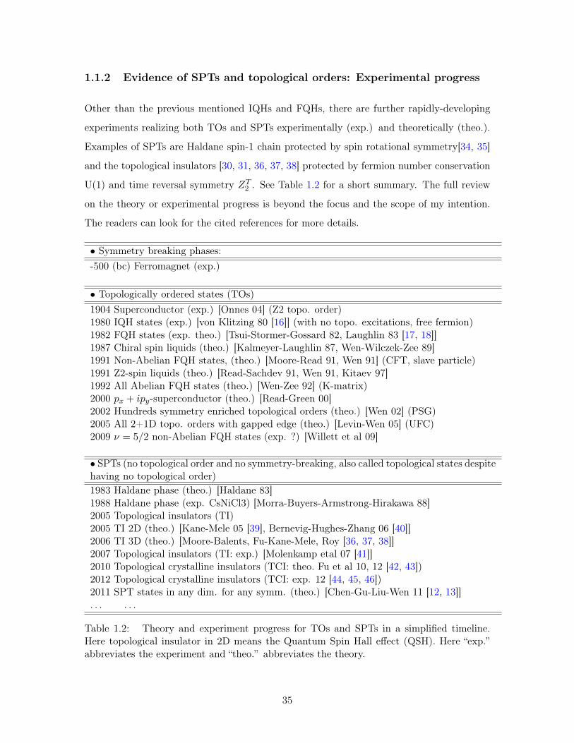
1.1.2 Evidence of SPTs and topological orders: Experimental progress
Other than the previous mentioned IQHs and FQHs, there are further rapidly-developing
experiments realizing both TOs and SPTs experimentally (exp.) and theoretically (theo.).
Examples of SPTs are Haldane spin-1 chain protected by spin rotational symmetry[34, 35]
and the topological insulators [30, 31, 36, 37, 38] protected by fermion number conservation
U(1) and time reversal symmetry 𝑍𝑇2 . See Table 1.2 for a short summary. The full review
on the theory or experimental progress is beyond the focus and the scope of my intention.
The readers can look for the cited references for more details.
∙ Symmetry breaking phases:-500 (bc) Ferromagnet (exp.)
∙ Topologically ordered states (TOs)1904 Superconductor (exp.) [Onnes 04] (Z2 topo. order)1980 IQH states (exp.) [von Klitzing 80 [16]] (with no topo. excitations, free fermion)1982 FQH states (exp. theo.) [Tsui-Stormer-Gossard 82, Laughlin 83 [17, 18]]1987 Chiral spin liquids (theo.) [Kalmeyer-Laughlin 87, Wen-Wilczek-Zee 89]1991 Non-Abelian FQH states, (theo.) [Moore-Read 91, Wen 91] (CFT, slave particle)1991 Z2-spin liquids (theo.) [Read-Sachdev 91, Wen 91, Kitaev 97]1992 All Abelian FQH states (theo.) [Wen-Zee 92] (K-matrix)2000 𝑝𝑥 + 𝑖𝑝𝑦-superconductor (theo.) [Read-Green 00]2002 Hundreds symmetry enriched topological orders (theo.) [Wen 02] (PSG)2005 All 2+1D topo. orders with gapped edge (theo.) [Levin-Wen 05] (UFC)2009 𝜈 = 5/2 non-Abelian FQH states (exp. ?) [Willett et al 09]
∙ SPTs (no topological order and no symmetry-breaking, also called topological states despitehaving no topological order)1983 Haldane phase (theo.) [Haldane 83]1988 Haldane phase (exp. CsNiCl3) [Morra-Buyers-Armstrong-Hirakawa 88]2005 Topological insulators (TI)2005 TI 2D (theo.) [Kane-Mele 05 [39], Bernevig-Hughes-Zhang 06 [40]]2006 TI 3D (theo.) [Moore-Balents, Fu-Kane-Mele, Roy [36, 37, 38]]2007 Topological insulators (TI: exp.) [Molenkamp etal 07 [41]]2010 Topological crystalline insulators (TCI: theo. Fu et al 10, 12 [42, 43])2012 Topological crystalline insulators (TCI: exp. 12 [44, 45, 46])2011 SPT states in any dim. for any symm. (theo.) [Chen-Gu-Liu-Wen 11 [12, 13]]. . . . . .
Table 1.2: Theory and experiment progress for TOs and SPTs in a simplified timeline.Here topological insulator in 2D means the Quantum Spin Hall effect (QSH). Here “exp.”abbreviates the experiment and “theo.” abbreviates the theory.
35
1.2 Motivations and Problems
1.2.1 Symmetry, Topology and Anomalies of Quantum Matter
With the background knowledge on quantum matter, let us now motivate in a colloquial style
of colloquium on how the symmetry, topology and anomalies can be involved in quantum
matter. This overview can guide us to pose new questions and the statement of the problems
in the next in Sec.1.2.2.
Symmetry, in everyday terms, means the system stays invariant under certain transfor-
mation. To describes the states of matter governed by symmetry, Ginzburg-Landau (G-L)
theory [8] semi-classically dictates the global symmetry realized onsite and locally. How-
ever, quantum wavefunctions become fuzzy due to Heisenberg’s uncertainty principle and
spread non-onsite. The symmetry operation can also act non-onsite — the symmetry con-
cept is enriched when understood at a fully quantum level. This new concept of non-onsite
symmetry can be realized on the boundary of some bulk gapped insulating phases, it un-
earths many missing states buried beneath G-L theory. States are identified via local-unitary
transformations, distinct new states are termed SPTs [12, 13].
Anomalies are phenomena that cannot be realized in their own spacetime dimensions.
A classical analogy is that two-dimensional (2D) waves propagate on the surface of the ocean
require some extended dimension, the 3D volume of bulk water. Similarly, quantum anoma-
lies describe the anomalous boundary physics at the quantum level [4] — the obstruction
to regularizing classical symmetries on the boundary quantized lattice without an extended
bulk. One of the earlier attempts on connecting quantum anomalies and topological defects
are done by Jackiw [6] and Callan-Harvey [47]. In their work, the use of field theory is
implicitly assumed to represent many-body quantum system. In my work, I will directly
establish the quantum anomalies realized on a discretized regularized lattice of many-body
quantum system.
The field theory regularization at high energy in HEP corresponds to the short distance
lattice cutoff in CMP. Using the lattice cutoff as a mean of regularization, we have the
advantage of distinguishing different types of global symmetry operations, namely onsite and
non-onsite. We learn that the quantum variables of onsite symmetry can be promoted to
dynamical ones and thus can be easily “gauged.” In contrast, non-onsite symmetry manifests
36
“short-range or long-range entangle” properties, hence hard to be gauged: it is an anomalous
symmetry. By realizing that such an obstruction to gauging a global symmetry coincides
with the ’t Hooft anomalies [48], we are led to the first lesson:
“The correspondence between non-onsite global symmetries and gauge anomalies.”
The correspondence is explicit at the weak gauge coupling. Ironically, we find that gauge
anomalies need only to be global symmetry anomalies. Gauge symmetries are not sym-
metries but redundancies; only global symmetries are real symmetries. Meanwhile, the
non-onsite symmetry is rooted in the SPT boundary property. Thus we realize the second
lesson:
“The correspondence between gauge anomalies and SPT boundary modes [49, 50].”
Topology, in colloquial terms, people may mistakenly associate the use of topology
with the twisting or the winding of electronic bands. More accurately, the topology should
be defined as a global property instead of local geometry, robust against any local pertur-
bations even those breaking all symmetries. Thus topological insulators and SPTs are not
really topological, due to their lack of robustness against short-range perturbations break-
ing their symmetry (see also Table 1.4). Our key observation is that since the boundary
gapless modes and anomalous global symmetries of SPTs are tied to gauge anomalies, the
further robust boundary gapless modes of intrinsic topological orders must be associated to
some anomalies requiring no global symmetry. We realize these anomalies violate space-
time diffeomorphism covariance on their own dimensions. This hints at our third lesson:
“The correspondence between gravitational anomalies and TO’s boundary modes [49, 51].”
Prior to our recent work [52], the previous two-decades-long study of topological orders in
the CMP community primarily focuses on 2D topological orders using modular SL(2,Z) data
[15]. Imagine a bulk topological phase of matter placed on a donut as a 2-torus; we deform
its space and then reglue it back to maintain the same topology. This procedure derives the
mapping class group MCG of a 2-torus 𝑇 2, which is the modular group MCG(𝑇 2)=SL(2,Z)
generated by an 𝒮 matrix via 90∘ rotation and a 𝒯 matrix via the Dehn twist. Modular
SL(2,Z) data capture the non-Abeliang geometric phases of ground states [53] and describe
the braiding statistics of quasiparticle excitations. Clearly topological orders can exist in
37

higher dimensional spacetime, such as 3+1D, what are their excitations and how to charac-
terize their braiding statistics? This is an ongoing open research direction.
Regularizing chiral fermion or chiral gauge theory on the lattice non-perturbatively is a
long-standing challenge, due to Nielsen-Ninomiya’s no-go theorem on the fermion-doubling
problem [54]. Mysteriously our particle physics Standard model is a chiral gauge theory, thus
the no-go theorem is a big challenge for us to bypass for understanding non-perturbative
strong interacting regime of particle physics. Fermion-doubling problem in the free fermion
language is basically saying that the energy band cross the zero energy even times in the
momentum 𝑘-space of Brillouin zone due to topological reason, thus with equal number
of left-right moving chiral modes — the fermions are doubled. It suggests that the HEP
no-go theorem is rooted in the CMP thinking. Providing that our enhanced understanding
through topological states of matter, can we tackle this challenge?
Moreover, the nontrivial bulk braiding statistics of excitations and the boundary quan-
tum anomalies have certain correspondence. Will the study of the bulk-edge correspondence
of TOs/SPTs not only guide us to understand exotic phases in CMP, but also resolve the
non-perturbative understanding of particle physics contents, the Standard Model and be-
yond in HEP problems?
1.2.2 Statement of the problems
The above discussion in Sec.1.2.1 had outlined our thinking and the strategy to solve certain
physics issues. But what exactly are the physics issues and problems? Here let us be more
specific and pin down them straightforwardly and clearly. In my thesis, I attempt to address
the six questions Q.I-VI below and analytically formulate an answer to them:
(Q.I). SPT invariant and its field-theory representation [29, 55]: Topological or-
ders (TOs) and SPTs are very different. For TOs, there are topology-dependent degenerate
ground states on a topology-nontrivial manifold (such as 𝑑-torus 𝑇 𝑑). We can transport the
ground states and determine the non-Abelian geometric phases generated in the coupling
constant moduli-space. More conveniently, we can overlap the wavefunctions to obtain the
amplitude data. These are the universal topological invariant of TOs. How about SPTs?
The challenge is that, with symmetry-protection and without symmetry-breaking, there is
only a unique ground state. Can we obtain the universal SPT invariants? If it is obtainable
from a lattice model, then, is there a field-theory representation of SPT invariants? Can
38
we recover the group-cohomology classification of SPT and more beyond than that using
continuous field theory approach?
(Q.II). Bosonic anomalies [56, 57]: Quantum anomalies occur in our real-world physics,
such as pion decaying to two photons via Adler-Bell-Jackiw chiral anomaly [58, 59]. Anoma-
lies also constrain beautifully on the Standard Model of particle physics, in particular to
the Glashow-Weinberg-Salam theory, via anomaly-cancellations of gauge and gravitational
couplings. The above two familiar examples of anomalies concern chiral fermions and con-
tinuous symmetry (e.g. U(1), SU(2), SU(3) in the weak coupling limit). Out of curiosity, we
ask: “Are there concrete examples of quantum anomalies for bosons instead? And anomalies
for discrete symmetries? Can they be formulated by a continuous field theory and a reg-
ularized lattice model? Are they potentially testable experimentally in the lab in the near
future?”
(Q.III). Topological gapping criteria. Topological degeneracy on a manifold with
gapped domain walls and boundaries [60, 61]: By now 2D topological orders are well-
studied. We understand the proper label of a single 2D topological order by a set of “topo-
logical invariants” or “topological order parameters”— the aforementioned modular SL(2,Z)
𝒮, 𝒯 matrices and the chiral central charge 𝑐−. The 𝒮, 𝒯 matrices can be derived from
geometric phases and encode the quasiparticle (or anyon) statistics. Non-zero chiral cen-
tral charge 𝑐− implies the topological gapless edge modes. However, it is less known how
separate topological orders are related. To this end, it is essential to study the following
circumstance: there are several domains in the system and each domain contains a topolog-
ical order, while the whole system is gapped. In this case, different topological orders are
connected by gapped domain walls. Under what criteria can two topological orders be con-
nected by a gapped domain wall, and how many different types of gapped domain walls are
there? Since a gapped boundary is a gapped domain wall between a nontrivial topological
order and the vacuum, we can meanwhile address that under what criteria can topological
orders allow gapped boundaries? When a topologically ordered system has a gapped bulk,
gapped domain walls and gapped boundaries, how to calculate its GSD on any orientable
manifold?
(Q.IV). Define lattice chiral fermion/gauge theory non-perturbatively [50]: The
Standard Model is a chiral gauge theory with chiral fermions — where the weak-interaction
39
gauge fields couple to the right-hand and the left-hand fermions differently. We know the
perturbative Lagrangian definition of the Standard Model since 1970. However, we do
not know whether the Standard Model can be regularized on the lattice, due to the Nielsen-
Ninomiya fermion-doubling no go theorem. And we do not have a non-perturbative definition
of Standard Model as a Hamiltonian quantum mechanical theory. We ask: “Whether there is
a local short-range finite quantum Hamiltonian system realizing onsite symmetry G defined
on a spatial lattice with a continuous time, such that its low energy physics produces a
anomaly-free chiral matter theory of symmetry G?”
(Q.V). String and particle exotic braiding statistics [52, 62]: Higher dimensional
topological orders are the new research frontier and are mostly not yet systematically ex-
plored. In 3+1D, the excitations can involve not only particle excitations but also string
excitations. We can ask: How to (at least partially) classify and characterize 3+1D topo-
logical orders? How to characterize the braiding statistics of strings and particles? How to
formulate or construct certain 3+1D topological orders on the lattice? What is the physical
interpretation of braiding statistics data?
(Q.VI). Topological invariants, as quantum statistics derived from spacetime
surgery [Chap.6]: We have mentioned that the mapping class group data from overlap-
ping the wavefunction from a spatial manifold mapped back to another wavefunction on
the same spatial manifold, such as the modular SL(2,Z) data 𝒮 and 𝒯 matrices on 𝑇 2-
torus, provide the universal topological invariants for topological orders (TOs). Now, we
can digest that, the (projective) representations of these modular transformation and the
mapping class group encode the information of TOs, thus encode the information of quan-
tum topology. However, it seems that the mapping class group, or more generally the spatial
topology dictates certain hidden rules governing the quantum topology. We can ask: How
the spacetime topology and the quantum topology are related or associated with each other?
Can the spacetime topology constrains the existence of certain quantum phases? Reversely,
or more profoundly and philosophically, can the quantum topology constrains the existence
of specific spacetime topology?
40
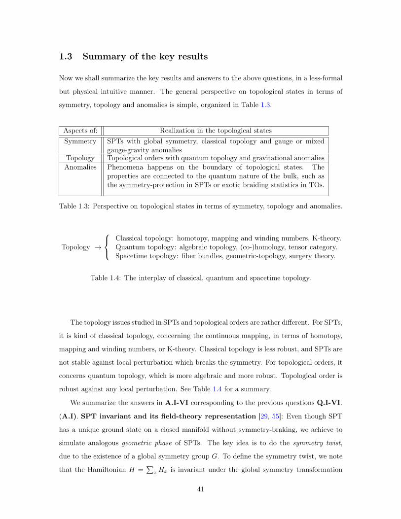
1.3 Summary of the key results
Now we shall summarize the key results and answers to the above questions, in a less-formal
but physical intuitive manner. The general perspective on topological states in terms of
symmetry, topology and anomalies is simple, organized in Table 1.3.
Aspects of: Realization in the topological statesSymmetry SPTs with global symmetry, classical topology and gauge or mixed
gauge-gravity anomaliesTopology Topological orders with quantum topology and gravitational anomaliesAnomalies Phenomena happens on the boundary of topological states. The
properties are connected to the quantum nature of the bulk, such asthe symmetry-protection in SPTs or exotic braiding statistics in TOs.
Table 1.3: Perspective on topological states in terms of symmetry, topology and anomalies.
Topology →
⎧⎨⎩Classical topology: homotopy, mapping and winding numbers, K-theory.Quantum topology: algebraic topology, (co-)homology, tensor category.Spacetime topology: fiber bundles, geometric-topology, surgery theory.
Table 1.4: The interplay of classical, quantum and spacetime topology.
The topology issues studied in SPTs and topological orders are rather different. For SPTs,
it is kind of classical topology, concerning the continuous mapping, in terms of homotopy,
mapping and winding numbers, or K-theory. Classical topology is less robust, and SPTs are
not stable against local perturbation which breaks the symmetry. For topological orders, it
concerns quantum topology, which is more algebraic and more robust. Topological order is
robust against any local perturbation. See Table 1.4 for a summary.
We summarize the answers in A.I-VI corresponding to the previous questions Q.I-VI.
(A.I). SPT invariant and its field-theory representation [29, 55]: Even though SPT
has a unique ground state on a closed manifold without symmetry-braking, we achieve to
simulate analogous geometric phase of SPTs. The key idea is to do the symmetry twist,
due to the existence of a global symmetry group 𝐺. To define the symmetry twist, we note
that the Hamiltonian 𝐻 =∑
𝑥𝐻𝑥 is invariant under the global symmetry transformation
41
𝑈 =∏
all sites 𝑈𝑥, namely 𝐻 = 𝑈𝐻𝑈−1. If we perform the symmetry transformation 𝑈 ′ =∏𝑥∈𝜕𝑅 𝑈𝑥 only near the boundary of a region 𝑅 (say on one side of 𝜕𝑅), the local term 𝐻𝑥
of 𝐻 in the Hamiltonian near the boundary of 𝑅 will be modified: 𝐻𝑥 → 𝐻 ′𝑥|𝑥 near 𝜕𝑅. It is
important to remark that the original symmetry 𝑈(𝑔) is local, unitary and onsite and has
a tensor product structure, but the symmetry-twist transformation is not unitary and not
a symmetry transformation. Instead, the symmetry-twist operation is a modification to the
original Hamiltonian. In short,
𝑈(𝑔) = ⊗𝑗𝑈𝑗(𝑔), 𝑈(𝑔)𝐻𝑈(𝑔)−1 = 𝐻, 𝑔 ∈ 𝐺.
𝐻 =∑𝑥
𝐻𝑥sym.twst along 𝜕𝑅−→
∑𝑥 ∈𝜕𝑅
𝐻𝑥 +∑𝑥∈𝜕𝑅
𝐻 ′𝑥|𝑥 near 𝜕𝑅 (1.1)
Suppose the branch cut 𝜕𝑅 is between the sites indices 𝑥0,𝑗 and 𝑥1,𝑗 varying 𝑗 while
moving along the 𝜕𝑅, and suppose the interacting Hamiltonian are nearest neighbored
interacting with the local term 𝐻𝑥𝑖,𝑥𝑗 . We stress that the symmetry twist can be per-
formed as part of symmetry transformation to modify 𝐻 ′𝑥 as 𝐻𝑥0,𝑗 ,𝑥1,𝑗 → 𝐻 ′
𝑥0,𝑗 ,𝑥1,𝑗 ≡
𝑈𝑥1,𝑗 (𝑔)𝐻𝑥0,𝑗 ,𝑥1,𝑗𝑈𝑥1,𝑗 (𝑔)−1, however the symmetry twist maintains 𝐻𝑥1,𝑗 ,𝑥2,𝑗 → 𝐻𝑥1,𝑗 ,𝑥2,𝑗 .
Thus overall the symmetry twist is not a symmetry transformation but a modification on
𝐻 to 𝐻 ′.
The above is a lattice Hamiltonian approach. Can we interpret in terms of a continuous
field theory perspective? For systems that realize topological orders, we can adiabatically
deform the ground state |Ψ𝑔.𝑠.(𝑔)⟩ of parameters 𝑔 via:
⟨Ψ𝑔.𝑠.(𝑔 + 𝛿𝑔)|Ψ𝑔.𝑠.(𝑔)⟩ ≃ . . .Z0 . . . (1.2)
to detect the volume-independent universal piece of spacetime partition function, Z0, which
reveals non-Abelian geometric phase of ground states. We can use Z0 with the symmetry
twist to probe the SPTs. A symmetry twist implies a change along a codimension-1 surface,
which modifies the SPT partition function from Z0 to Z0(sym.twist). Just like the geometric
phases of the degenerate ground states characterize topological orders [51], we believe that
Z0(sym.twist), on different spacetime manifolds and for different symmetry twists, fully
characterizes SPTs. The symmetry twist is similar to gauging the on-site symmetry except
that the symmetry twist is non-dynamical. We can use the gauge connection 1-form 𝐴 to
42
describe the corresponding symmetry twists, with probe-fields 𝐴 coupling to the matter
fields of the system. So we can write
Z0(sym.twist) = eiS0(sym.twist) = eiS0(𝐴). (1.3)
Here S0(𝐴) is the SPT invariant that we search for. This is a partition function of classical
probe fields, or a topological response theory, obtained by integrating out the matter fields
of SPTs path integral [29, 55].
(A.II). Bosonic anomalies [56, 57]: We classify and characterize several types of bosonic
anomalies found on the boundary of bosonic SPTs, as an example on 1+1D edge. One has
induced fractional quantum numbers via symmetry-breaking (similar to Jackiw-Rebbi [63]
and Goldstone-Wilczek [64] effects); one has degenerate zero modes (carrying the projective
representation protected by the unbroken part of the symmetry) either near the 0D kink of
a symmetry-breaking domain wall, or on a symmetry-preserving 1D system dimensionally
reduced from a thin 2D tube with a monodromy defect 1D line embedded. More generally,
the energy spectrum and conformal dimensions of gapless edge modes under an external
gauge flux insertion (or twisted by a branch cut, i.e., a monodromy defect line) through the
1D ring can distinguish many SPT classes. The last one exhibits the many-body Aharonov-
Bohm (A-B) effect [57]. The aforementioned edge properties are explicitly formulated in
terms of (i) a long wavelength continuum field theory involving scalar chiral bosons [65,
66, 67, 56], for a generic finite Abelian symmetry group 𝐺 =∏𝑢 𝑍𝑁𝑢 . We can express the
multiplet (non-)chiral boson action S𝑒𝑑𝑔𝑒 =∫𝐾𝐼𝐽4𝜋 𝑑𝑡𝑑𝑥 𝜕𝑡𝜑𝐼𝜕𝑥𝜑𝐽 with a 𝐾-matrix: 𝐾 =(
0 11 0
)⊕(0 11 0
)⊕(0 11 0
)⊕ . . . , and a multiplet of scalar bosons: 𝜑𝐼 = (𝜑1, 𝜑
′1, 𝜑2, 𝜑
′2, . . . ) with
chiral-anti-chiral pair of scalar modes (𝜑𝑢, 𝜑′𝑢). One of our key formulas is the symmetry
operator 𝑆 completing the group cohomology classification,
𝑆 =∏
𝑢,𝑣,𝑤∈{1,2,3}
exp[ i 2𝜋𝑁𝑢
∫ 𝐿
0𝑑𝑥 (
1
2𝜋𝜕𝑥𝜑
′𝑢 +
𝑝I
2𝜋𝜕𝑥𝜑𝑢
+ 𝜖𝑢𝑣𝑝II
2𝜋𝜕𝑥𝜑𝑣 +
𝑝III𝑁1𝑁2𝑁3
(2𝜋)2𝑁123𝜖𝑢𝑣𝑤𝜑𝑤(𝑥) · 𝜕𝑥𝜑𝑣(𝑥))
], (1.4)
where 𝑝I, 𝑝II, 𝑝III are nontrivial SPT class indices. Here our discrete formulations: (ii) Matrix
Product Operators and (iii) discrete quantum lattice models provide crucial insights to derive
(i) the field theory formulation. The symmetry transformation can be readily checked by
43
calculating 𝑆𝜑𝐼𝑆−1 with the commutation relations given above. Our lattice approach yields
a regularization with anomalous non-onsite symmetry for the field theory description.
(A.III). Topological gapping criteria. Topological degeneracy on a manifold with
gapped domain walls and boundaries [60, 61]. The observation in the third lesson
guides us to study, under what mechanisms, would edge modes protected to be gapless: (i)
the chirality, associated with perturbative gravitational anomalies and gauge anomalies; (ii)
the global symmetry protection; (iii) the bulk nontrivial statistics [60, 68]: even for non-
chiral states, global gravitational anomalies can protect gapless edge modes [61]. Conversely,
to determine the edge mode gapping criteria of TOs, we use both TQFT [60] as well as using
SL(2,Z) modular data and category theory [61]. Once the boundary modes are gapped, we
can introduce the new concept of boundary degeneracy for ground states on a generic (open
or closed) manifold of gapped boundaries and domain walls [60, 68], which provides richer
information than the old concept of bulk degeneracy on a closed manifold. Intuitively a
gapped boundary is labeled by a set of anyons where they share trivial self and mutual
braiding statistics. We can call this set of particles as condensible particles. In the Abelian
TOs, this set of anyons, with the fusion as operator, form a mathematical group structure
like a lattice.2 We derive the GSD for TOs on a manifold with gapped boundaries, here in
an intuitive simplified level, as the order of a quotient group between two lattices of Hilbert
space,
GSD =
lattice of condensible anyons
lattice of condensible non-fractionalized particles
, (1.5)
subject to the implicit constraint on neutrality condition of anyon transporting between all
gapped boundaries. Our generic result of boundary GSD recovers the known result of bulk
GSD for a level 𝑘 or 𝐾-matrix Chern-Simons theory (𝑘 = 3 for a filling-fraction 13 -FQH
state discussed in Sec.1.1.1) with
GSD = 𝑘𝑔, or | det𝐾|𝑔.
on a genus 𝑔-Riemman surface. We predict that the 𝑍2 toric code [69] and 𝑍2 double-semion
model (more generally, the 𝑍𝑘 gauge theory and the 𝑈(1)𝑘 × 𝑈(1)−𝑘 non-chiral fractional
quantum Hall state at even integer 𝑘) can be numerically and experimentally distinguished,
by measuring their boundary degeneracy on an annulus or a cylinder. For a more generic
2For experts in Chern-Simons TQFT, it is the Chern-Simons quantized lattice Hilbert space.
44
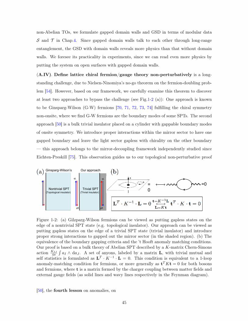
non-Abelian TOs, we formulate gapped domain walls and GSD in terms of modular data
𝒮 and 𝒯 in Chap.4. Since gapped domain walls talk to each other through long-range
entanglement, the GSD with domain walls reveals more physics than that without domain
walls. We foresee its practicality in experiments, since we can read even more physics by
putting the system on open surfaces with gapped domain walls.
(A.IV). Define lattice chiral fermion/gauge theory non-perturbatively is a long-
standing challenge, due to Nielsen-Ninomiya’s no-go theorem on the fermion-doubling prob-
lem [54]. However, based on our framework, we carefully examine this theorem to discover
at least two approaches to bypass the challenge (see Fig.1-2 (a)): One approach is known
to be Ginsparg-Wilson (G-W) fermions [70, 71, 72, 73, 74] fulfilling the chiral symmetry
non-onsite, where we find G-W fermions are the boundary modes of some SPTs. The second
approach [50] is a bulk trivial insulator placed on a cylinder with gappable boundary modes
of onsite symmetry. We introduce proper interactions within the mirror sector to have one
gapped boundary and leave the light sector gapless with chirality on the other boundary
— this approach belongs to the mirror-decoupling framework independently studied since
Eichten-Preskill [75]. This observation guides us to our topological non-perturbative proof
qL
qR
qL
qR
Our approach Ginsparg-Wilson’s
Trivial SPT (Trivial insulator)
Nontrivial SPT (Topological insulator)
=0
=0
Figure 1-2: (a) Gilzparg-Wilson fermions can be viewed as putting gapless states on theedge of a nontrivial SPT state (e.g. topological insulator). Our approach can be viewed asputting gapless states on the edge of a trivial SPT state (trivial insulator) and introduceproper strong interactions to gapped out the mirror sector (in the shaded region). (b) Theequivalence of the boundary gapping criteria and the ’t Hooft anomaly matching conditions.Our proof is based on a bulk theory of Abelian SPT described by a 𝐾-matrix Chern-Simonsaction 𝐾𝐼𝐽
4𝜋
∫𝑎𝐼 ∧ d𝑎𝐽 . A set of anyons, labeled by a matrix L, with trivial mutual and
self statistics is formulated as L𝑇 · 𝐾−1 · L = 0. This condition is equivalent to a 1-loopanomaly-matching condition for fermions, or more generally as t𝑇𝐾t = 0 for both bosonsand fermions, where t is a matrix formed by the charger coupling between matter fields andexternal gauge fields (as solid lines and wavy lines respectively in the Feynman diagram).
[50], the fourth lesson on anomalies, on
45
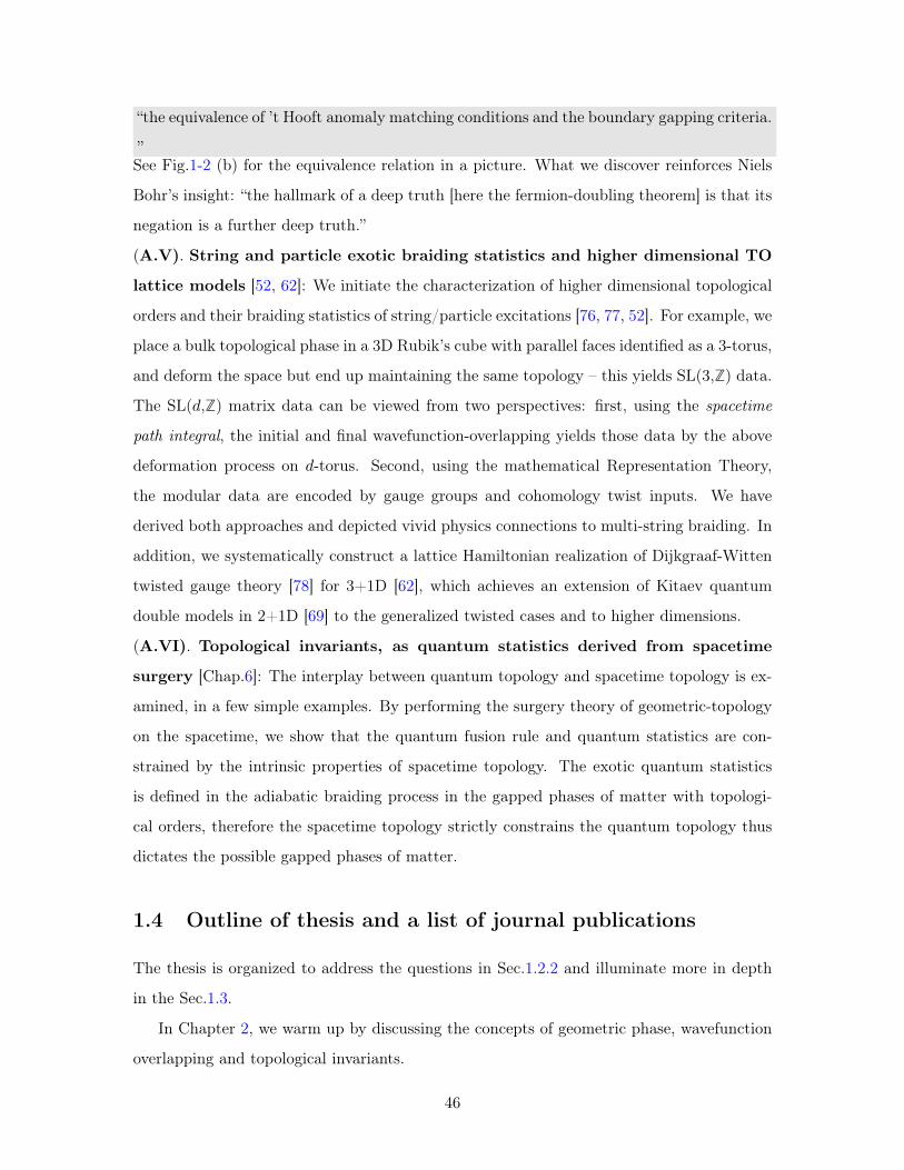
“the equivalence of ’t Hooft anomaly matching conditions and the boundary gapping criteria.
”See Fig.1-2 (b) for the equivalence relation in a picture. What we discover reinforces Niels
Bohr’s insight: “the hallmark of a deep truth [here the fermion-doubling theorem] is that its
negation is a further deep truth.”
(A.V). String and particle exotic braiding statistics and higher dimensional TO
lattice models [52, 62]: We initiate the characterization of higher dimensional topological
orders and their braiding statistics of string/particle excitations [76, 77, 52]. For example, we
place a bulk topological phase in a 3D Rubik’s cube with parallel faces identified as a 3-torus,
and deform the space but end up maintaining the same topology – this yields SL(3,Z) data.
The SL(𝑑,Z) matrix data can be viewed from two perspectives: first, using the spacetime
path integral, the initial and final wavefunction-overlapping yields those data by the above
deformation process on 𝑑-torus. Second, using the mathematical Representation Theory,
the modular data are encoded by gauge groups and cohomology twist inputs. We have
derived both approaches and depicted vivid physics connections to multi-string braiding. In
addition, we systematically construct a lattice Hamiltonian realization of Dijkgraaf-Witten
twisted gauge theory [78] for 3+1D [62], which achieves an extension of Kitaev quantum
double models in 2+1D [69] to the generalized twisted cases and to higher dimensions.
(A.VI). Topological invariants, as quantum statistics derived from spacetime
surgery [Chap.6]: The interplay between quantum topology and spacetime topology is ex-
amined, in a few simple examples. By performing the surgery theory of geometric-topology
on the spacetime, we show that the quantum fusion rule and quantum statistics are con-
strained by the intrinsic properties of spacetime topology. The exotic quantum statistics
is defined in the adiabatic braiding process in the gapped phases of matter with topologi-
cal orders, therefore the spacetime topology strictly constrains the quantum topology thus
dictates the possible gapped phases of matter.
1.4 Outline of thesis and a list of journal publications
The thesis is organized to address the questions in Sec.1.2.2 and illuminate more in depth
in the Sec.1.3.
In Chapter 2, we warm up by discussing the concepts of geometric phase, wavefunction
overlapping and topological invariants.
46
In Chapter 3, on Aspects of Symmetry, we address the issue in Q.I and A.I on the
procedure to do the symmetry-twist, on the SPT invariant derived from the lattice model or
and its field-theory representation. We also address part of the issues in Q.II and A.II on
bosonic anomalies and their SPT invariants and SPT observables. The reason we discuss part
of anomaly issue here is that remarkably the anomalous edge global symmetry corresponds
to the (gauge) anomalies. The global symmetry can be coupled to a weakly-coupling gauge
fields or external probe fields. So anomalous symmetries manifest quantum anomalies. The
issues of anomalous symmetry and anomalies are intertwined.
In Chapter 4, on Aspects of Topology, we work out Q.III and A.III, topological gapping
criteria, topological degeneracy on a manifold with gapped domain walls and boundaries.
We tackle the challenge of Q.V and A.V on string and particle exotic braiding statistics and
TO lattice models in 3+1D.
In Chapter 5, on Aspects of Anomalies, we address Q.IV and A.IV on a non-perturbative
definition of lattice chiral fermion/gauge theory. Other part of discussions are extension of
previous topics from Q.I and A.I on SPT field-theory representation with mixed gauge-
gravity anomalies, and Q.II and A.II on bosonic anomalies.
In Chapter 6, we address the issue in Q.VI and A.VI on quantum statistics data as
topological invariants derived from spacetime surgery. We formulate the constraints of
braiding statistics and fusion analogous to Verlinde’s formula in 2+1D and 3+1D. This
approach should be applicable to any spacetime dimension. A more complete study will be
reported elsewhere in the future publication.
Review articles: For a colloquium overview of topological insulators and supercon-
ductors can be found in [30, 31]. An earlier version of overview on topological phases is
in [32]. An intuitive but less-formal guide to topological insulators and SPTs can be found
in [33]. A more recent review on topological order is in [15]. Obviously I must thank S.
Coleman’s wonderful book [2] and its inspiration on my thesis and its title. Two impor-
tant reviews on quantum field theory and anomalies: Treiman-Witten-Jackiw-Zumino[4]
and Farhi-Jackiw[3].
Part of the thesis is the overview and the summary for part of the work published
elsewhere.
1. Juven Wang and Xiao-Gang Wen. Boundary Degeneracy of Topological Order. Phys.Rev.,
B91(12):125124, 2015. ArXiv e-prints 1212.4863. [60]
47
2. Peng Ye and Juven Wang. Symmetry-protected topological phases with charge and
spin symmetries: Response theory and dynamical gauge theory in two and three di-
mensions. Phys.Rev., B88(23):235109, 2013. ArXiv e-prints 1306.3695. [67]
3. Juven Wang and Xiao-Gang Wen. A Lattice Non-Perturbative Hamiltonian Con-
struction of 1+1D Anomaly-Free Chiral Fermions and Bosons - on the equiva- lence of
the anomaly matching conditions and the boundary fully gapping rules. 2013. ArXiv
e-prints 1307.7480. [50]
4. Luiz H. Santos and Juven Wang. Symmetry-protected many-body Aharonov- Bohm
effect. Phys.Rev., B89(19):195122, 2014. ArXiv e-prints 1310.8291[57]
5. Juven Wang, Luiz H. Santos, and Xiao-Gang Wen. Bosonic Anomalies, Induced Frac-
tional Quantum Numbers and Degenerate Zero Modes: the anomalous edge physics
of Symmetry-Protected Topological States. 2014. ArXiv e-prints 1403.5256 [56]
6. Juven Wang and Xiao-Gang Wen. Non-Abelian string and particle braiding in topo-
logical order: Modular SL(3,Z) representation and (3+1) -dimensional twisted gauge
theory. Phys.Rev., B91(3):035134, 2015. ArXiv e-prints 1404.7854 [52]
7. Juven C. Wang, Zheng-Cheng Gu, and Xiao-Gang Wen. Field theory represen- tation
of gauge-gravity symmetry-protected topological invariants, group coho- mology and
beyond. Phys.Rev.Lett., 114(3):031601, 2015. ArXiv e-prints 1405.7689 [79]
8. Tian Lan, Juven C. Wang, and Xiao-Gang Wen. Gapped Domain Walls, Gapped
Boundaries and Topological Degeneracy. Phys.Rev.Lett., 114(7):076402, 2015. ArXiv
e-prints 1408.6514 [61]
9. Yidun Wan, Juven C. Wang, and Huan He. Twisted Gauge Theory Model of Topo-
logical Phases in Three Dimensions. 2014. ArXiv e-prints 1409.3216 [62]
10. Zheng-Cheng Gu, Juven C. Wang, and Xiao-Gang Wen. Multi-kink topolog- ical terms
and charge-binding domain-wall condensation induced symmetry- protected topologi-
cal states: Beyond Chern-Simons/BF theory. 2015 ArXiv e-prints 1503.01768 [55]
11. Juven C. Wang, Clifford H. Taubes, Xiao-Gang Wen and Shing-Tung Yau. Quantum
statistics and spacetime surgery: Fusion algebra, braiding statistics, and mapping class
group (to appear)
48

and other work to appear in near-future publications.
49

50
Chapter 2
Geometric phase, wavefunction
overlap, spacetime path integral and
topological invariants
2.1 Overview
In this chapter, we work through the familiar concept of geometric phase, firstly emphasized
by Berry. The hint and the similar idea have been noticed by Pancharatnam, Aharonov-
Bohm and others that there is an extra geometric phase in addition to the familiar dynam-
ical phase when we perform the adiabatic evolution on the physical system governed by
Hamiltonian. What Berry emphasized is that when the adiabatic evolution trajectory in
the Hamiltonian coupling constant space is closed, then this trajectory-dependent geometric
phase is a physical measurable invariant quantity— this particular geometric phase is invari-
ant in a sense of gauge invariance. Wilczek-Zee noticed the non-Abelian geometric matrix
for adiabatically evolving degenerate states. Wen had the insights to discover topological
orders (TOs) and its GSD for quantum Hall fluids and apply the non-Abelian geometric
matrix together with Chern-Simons theory of Witten’s TQFT to characterize and classify
TOs. Here we digest the development of these ideas in a coherent physical way, and will
develop this approach further to study TOs and SPTs in any dimensions in Chap.3, 4 and
6.
51
2.2 Geometric (Berry’s) phase and the non-Abelian structure
2.2.1 Geometric (Berry’s) phase
Start with the study of wavefunction Ψ(𝜏(𝑡)) evolving under the time-dependent Hamilto-
nian 𝐻 = 𝐻(𝜏(𝑡)) of some time-dependent coupling constant 𝜏 . In general, for a series of 𝜏𝛼
parameters, we will simply denote them as the parameter 𝜏 . Our goal is determine Ψ(𝜏(𝑡))
by solving
𝐻|Ψ(𝜏(𝑡))⟩ = i~ 𝜕𝑡|Ψ(𝜏(𝑡))⟩.
Let us assume Ψ(𝜏(𝑡)) starts at 𝑡 = 0 from an energy-eigenstate Ψ(𝜏(0)) = 𝜑(𝜏(0)) ≡
𝜑𝐸0(𝜏(𝑡)) with an eigen-energy 𝐸0. At every moment we can still find a set of eigenstate
𝜑(𝜏(𝑡)) as bases following 𝐻(𝜏(𝑡))𝜑(𝜏(𝑡)) = 𝐸(𝜏(𝑡))𝜑(𝜏(𝑡)).
We consider the adiabatic evolution (without sudden exchange energy with external
environment), here in the sense that the time scale 𝑑𝑡 of changing the energy 𝑑𝐸 are bounded
between two other scales. One scale is the energy gap of higher/lower excitations, defined
as Δ ≃ Δ𝑗 ≡ |𝐸𝑗 −𝐸0|. The other scale is the energy splitting 𝛿 between nearly degenerate
ground states around the energy scale 𝐸0.1 The adiabatic evolution requires that the energy
changes at the unit time: d𝐸d𝑡 × unit time ≡ 𝜖 and the rate of change for a unit energy:
d𝐸d𝑡·unit energy ≡ 1/𝑇 are bounded by:
Δ≫ 𝑇−1 ≃ 𝜖, or equivalently Δ−1 ≪ 𝑇 ≃ 𝜖−1. (2.1)
How the scale 𝛿 is set in depends on the physics we look for. If we like to focus on a single
eigenstate without being interfered by other nearly degenerate states, then we will have to
set a finer condition: Δ > 𝛿 ≫ 𝑇−1 ≃ 𝜖, or equivalently, Δ−1 < 𝛿−1 ≪ 𝑇 ≃ 𝜖−1. Indeed,
this is difficult, and it will be easier if we start with an isolated eigenstate instead of the
troublesome nearly degenerate states! However, one interesting piece of physics emerges
when we consider the nearly degenerate states together. We will explore in Sec.2.2.2, the
geometric phase becomes non-Abelian if we are in the time scale where all nearly degenerate
1 A deep side remark: For some miraculous situation, say, ground states of certain many-body systemssuch as topological orders, the degenerate states are topologically robust to stay together as nearly degeneratein the energy spectrum. However, to hold the nearly degenerate into an exact degeneracy requires someextra symmetry. This extra symmetry may not be robust against local perturbation, and this symmetry isnot required for topological orders. In other words, the topological ground state degeneracy is not an exactdegeneracy, but only an approximate degeneracy !
52
states are important:
Δ≫ 𝑇−1 ≃ 𝜖≫ 𝛿, or equivalently Δ−1 ≪ 𝑇 ≃ 𝜖−1 ≪ 𝛿−1. (2.2)
Now let us stick to the simplest condition Eq.(2.1) for a moment with an isolated eigen-
state. We will generalize it to degenerate states in Sec.2.2.2. In this adiabatic evolution,
it is reasonable to write a generic wavefunction Ψ(𝜏(𝑡)) = e−i~∫ 𝑡0 d𝑠𝐸0(𝑠) · e i𝛾 · 𝜑(𝜏(𝑡)). The
first piece is dynamical phase which exists even for a time-independent Hamiltonian. The
second piece e i𝛾 can be solved, and one finds the geometric phase:
𝛾 =
∫ 𝜏(𝑡)
𝜏(0)d𝜏𝛼⟨𝜑(𝜏(𝑡))| i 𝜕
𝜕𝜏𝛼|𝜑(𝜏(𝑡))⟩ (2.3)
Several properties of 𝛾 are derived:
(i) 𝛾 is a pure phase, 𝛾 ∈ R because ⟨𝜑| dd𝜏 |𝜑⟩ is an imaginary number. The wavefunction
maintains unitary in the same eigenstate.
(ii) It has no explicit ~-dependence. So we may say the geometric phase remains even at
the classical limit ~→ 0.
(iii) It is geometric and trajectory-dependent. But it has no explicit time-dependent and it
is parametrization independent to 𝜏 , thus 𝛾 does not change no matter how fast or slow
the process is as long as the process stays adiabatic. In contrast, the dynamical phase is
explicitly time-dependent.
(iv) It can be written in terms of gauge potential as𝐴 ≡ 𝐴𝛼d𝜏𝛼 = ⟨𝜑(𝜏(𝑡))| i 𝜕𝜕𝜏𝛼 |𝜑(𝜏(𝑡))⟩d𝜏
𝛼,
so 𝛾 =∫ 𝜏(𝑡)𝜏(0) 𝐴 =
∫ 𝜏(𝑡)𝜏(0) d𝜏
𝛼 𝐴(𝜏)𝛼. In the most general case, 𝐴 is a connection on a U(1)-
bundle with a base-manifold in the 𝜏 -parameter space. If the U(1)-bundle is trivial, the
connection 𝐴 becomes a Lie-algebra valued 1-form, more specifically a 1-form gauge field.
(v) A choice of eigenbasis up to U(1) phase becomes the gauge transformation, if we change
the eigenstate by a unitary transformation 𝜑′(𝜏) = Ω(𝜏)𝜑(𝜏) where Ω−1Ω = Ω†Ω = 1, then
the gauge field 𝐴′ = 𝐴 + i(dΩ)Ω−1 ⇒ 𝐴′𝛼 = 𝐴𝛼 + i( 𝜕
𝜕𝜏𝛼Ω)Ω−1. For a single energy level,
Ω(𝜏) = e i𝑓(𝜏), so the gauge field is transformed as 𝐴′ = 𝐴− d𝑓 .
(vi) A universal feature of the geometric phase 𝛾 arises, if the trajectory is closed with an
enclosed region 𝑅. Namely, because∮d𝑓 = 0, the 𝛾 does not depend on the choices
of eigenbasis and the basis (“gauge”) transformation. If there are multiple parameters
of 𝜏𝛼 = (𝜏1, 𝜏2, . . . ), we further define the field strength as: 𝐹𝛼𝛽 = 𝜕𝛼𝐴𝛽 − 𝜕𝛽𝐴𝛼 =
53
i(⟨ 𝜕𝜑𝜕𝜏𝛼 |𝜕𝜑𝜕𝜏𝛽⟩ − ⟨ 𝜕𝜑
𝜕𝜏𝛽| 𝜕𝜑𝜕𝜏𝛼 ⟩), so
𝛾enclosed =
∮𝜕𝑅𝐴 =
∮𝜕𝑅𝐴(𝜏)𝛼d𝜏
𝛼 =
∫𝑅𝐹 =
∫𝑅𝐹𝛼𝛽 d𝜏
𝛼 ∧ d𝜏𝛽 (2.4)
However, we stress and clarify that the 1-form “gauge field” 𝐴 and the 2-form “field-strength
curvature” 𝐹 here are not those in the usual dynamical gauge theory, since it lives in the
probed coupling constant 𝜏 with values determined by semi-classical external probes.
(vii) We can rewrite the geometric phase 𝛾 in terms of Kubo formula or the linear response
theory form. Insert a complete eigenbasis identity matrix 𝐼 =∑
𝐸𝑗|𝜑𝐸𝑗 ⟩⟨𝜑𝐸𝑗 | into the 𝐹𝛼𝛽-
term (be aware, not just for the single eigenstate or nearly degenerate states with energy
𝐸0(𝜏(𝑡)), but the whole energy spectrum 𝐸𝑗) and then use the analogous Hellmann-Feynman
relation ⟨𝜑𝐸𝑗 | 𝜕𝐻𝜕𝜏𝛼 |𝜑𝐸0⟩+ (𝐸𝑗 − 𝐸0)⟨𝜑𝐸𝑗 |𝜕𝜑𝐸0𝜕𝜏𝛼 ⟩, plug in Eq.(2.4), we obtain:
𝛾enclosed = i
∫𝑅(⟨𝜕𝜑𝐸0
𝜕𝜏𝛼|𝜕𝜑𝐸0
𝜕𝜏𝛽⟩ − ⟨𝜕𝜑𝐸0
𝜕𝜏𝛽|𝜕𝜑𝐸0
𝜕𝜏𝛼⟩)d𝜏𝛼 ∧ d𝜏𝛽 (2.5)
= i
∫𝑅
∑𝑗
⟨𝜑𝐸0 | 𝜕𝐻𝜕𝜏𝛼 |𝜑𝐸𝑗 ⟩⟨𝜑𝐸𝑗 | 𝜕𝐻𝜕𝜏𝛽 |𝜑𝐸0⟩ − ⟨𝜑𝐸0 | 𝜕𝐻𝜕𝜏𝛽 |𝜑𝐸𝑗 ⟩⟨𝜑𝐸𝑗 | 𝜕𝐻𝜕𝜏𝛼 |𝜑𝐸0⟩(𝐸𝑗 − 𝐸0)2
d𝜏𝛼 ∧ d𝜏𝛽. (2.6)
We will comment more on the deeper meanings of Eq.(2.5) and Eq.(2.6) after introducing
the more general non-Abelian geometric matrix structure (also called non-Abelian Berry
phase or non-Abelian gauge structure) emerged in degenerate energy states.
2.2.2 Non-Abelian Geometric (Berry’s) Structure
We can generalize the approach above to the case with 𝑁 -fold degenerate energy states of
energy 𝐸0, firstly performed by Wilczek and Zee [53]. For degenerate states |𝜑𝐸0,𝑎⟩ ≡ |𝜑𝑎⟩
with 𝑎 = 1, . . . , 𝑁 , we define the 1-form gauge field as
𝐴 = 𝐴𝑏𝑎,𝛼d𝜏𝛼 = ⟨𝜑𝑎(𝜏)| i
𝜕
𝜕𝜏𝛼|𝜑𝑏(𝜏)⟩d𝜏𝛼 (2.7)
We can prove that 𝐴𝑎𝑏 is Hermitian: 𝐴𝑎𝑏 = 𝐴*𝑏𝑎. If the coupling 𝜏 is defined to be real,
we have 𝐴 = 𝐴†. The gauge transformation becomes an Ω(𝜏) transformation between
degenerate states: |𝜑′𝑎⟩ = Ω𝑎𝑏|𝜑𝑏⟩. We find 𝐴′𝑏𝑎,𝛼 = Ω𝑏𝑑𝐴𝑑𝑐(Ω
−1)𝑐𝑎 + i( 𝜕𝜕𝜏𝛼Ω𝑏𝑐)(Ω
−1)𝑐𝑎,
namely,
𝐴′ = Ω𝐴Ω−1 + i(dΩ)(Ω−1). (2.8)
54
(viii) 𝛾 as a rank-𝑁 matrix : The geometric meaning of Eq.(2.4) still holds for non-Abelian
geometric structure, where 𝛾 now becomes a rank-𝑁 matrix 𝛾𝑏𝑎 for 𝑁 -degenerate states
at 𝐸0. The geometric phase factor e i𝛾 for Schrödinger equation becomes a non-Abelian
rank-𝑁 matrix:
[e i𝛾 ]𝑏𝑎 = P[e i∫𝐴𝛼 d𝜏𝛼 ]𝑏𝑎 (2.9)
with the path ordering P. For 𝑁 -degenerate states, we can generalize Eq.(2.5) and Eq.(2.6)
by replacing |𝜑𝐸0⟩ by |𝜑𝐸0,𝑎⟩ = |𝜑𝐸0,𝑎⟩. The modification of Eq.(2.6) requires a higher order
perturbation theory to fix the singular 𝑂((𝐸𝑗−𝐸0)−2) piece, but the term written in Eq.(2.6)
still exists for 𝐸𝑗 = 𝐸0.
(ix) We remark that the meanings of Eq.(2.5) and Eq.(2.6) are rather different. First,
Eq.(2.5) only evaluates the single eigenstate |𝜑𝐸0⟩ or nearly degenerate states |𝜑𝐸0,𝑖⟩ with
the same energy 𝐸0, and study its-trajectory enclosed region 𝑅’s local curvature 𝐹 in the
Hamiltonian coupling constant space. Second, the form in Eq.(2.6) with a second-order
perturbation form 𝑂((𝐸𝑗 − 𝐸0)−2) is associated to the fact that the curvature 𝐹 has a
second-order derivative. However, Eq.(2.6) also gather extra information about the nearby
higher/lower energy excitations |𝜑𝐸𝑗 ⟩, the variation of the full Hamiltonian 𝜕𝐻𝜕𝜏𝛼 , and how
dense these excitations with energy 𝐸𝑗 are around 𝐸0 in the spectrum.
We stress that, from Eq.(2.5) and Eq.(2.6) and the remark (ix),
Geometric phase captures important properties encoded in the target eigenstates, (such
as degenerate ground states, say |𝜑𝐸0,𝑖⟩) as in Eq.(2.4) and (2.5). Moreover, geometric
phase also encodes information about the nearby excitation states, as in Eq.(2.6). In
Chap.4 we will utilize this fact to compute the Abelian or non-Abelian braiding statistics
of energetic excitations of strings and particles by studying the geometric phase or
non-Abelian geometric structure of degenerate ground states. Non-Abelian geometric
structure only means that 𝛾 is a matrix, the braiding statistics can still be Abelian or
non-Abelian statistics.
We remark on the parametrization of the parameter space:
55
The usual gauge theory has a form 𝐴 = 𝐴𝜇(𝑥)d𝑥𝜇 with explicit spacetime dependence
𝑥𝜇, for a gauge group 𝐺, then the 𝐴 is a connection of a 𝐺-bundle. The “gauge field”
𝐴 = 𝐴(𝜏)𝛼d𝜏𝛼 we study depends on the Hamiltonian coupling constant 𝜏 space. The
“gauge group’ depends on the accidental global symmetry of degenerate ground states.
such as U(𝑁) = U(1)×SU(𝑁) for 𝑁 -fold degeneracy. The state |Ψ⟩ lives in the Hilbert
space.
2.3 Quantum Hall Liquids: From one electron to many elec-
trons on the torus to the effective Chern-Simons theory
Here we like to introduce an additional idea, to use the Berry phase and geometric matrix
structure to characterize and classify 2D quantum Hall liquids. For an interacting system
with 𝑁 electrons described by the toy-model Hamiltonian [80]:
𝐻 = −1
2
~2
𝑚𝑒
𝑁∑𝑖
(𝜕��𝑖 − i��(��𝑖))2 +
∑𝑖<𝑗
𝑉𝐾(��𝑖 − ��𝑗), (2.10)
with a higher order derivative interacting potential 𝑉𝐾(��) ≡∑𝐾
𝑛=1 𝑣𝑛(−1)𝑛𝜕𝑛𝑧 𝛿(𝑧)𝜕𝑛𝑧 . The
coordinates of 𝑖-th electron is 𝑧𝑖 ≡ 𝑥𝑖 + i𝑦𝑖. On the other hand, Laughlin wavefunction was
proposed to be an ansatz for the FQHs with a filling fraction 𝜈 = 1/𝐾:
Ψ𝐾({𝑧𝑖}) =[∏
(𝑧𝑖 − 𝑧𝑗)𝐾]e− 1
4ℓ2𝐵
∑|𝑧𝑖|2
, (2.11)
with ℓ𝐵 =√
~𝑐/𝑒𝐵 and 2𝜋ℓ2𝐵𝐵 = ℎ𝑐/𝑒 = Φ0 as a unit flux. It is an only approximate
ansatz for the real system, because it does not take into account a finite size system with
a finite radius confining potential and the Coulomb interactions. However, the Laughlin
wavefunction turns out to be an exact ground state of the above Hamiltonian on a 2D
plane for an appropriate vector potential �� = 12(−𝐵𝑦,𝐵𝑥) in a symmetric gauge and the
background magnetic field 𝐵. More generally, we can consider a single or multilayer many-
body electronic systems as a FQHs described by a wavefunction with a 𝐾𝐼𝐽 𝐾-matrix data,
Ψ𝐾𝐼𝐽({𝑧𝑖}) =
[∏(𝑧
(𝐼)𝑖 − 𝑧
(𝐽)𝑗 )𝐾𝐼𝐽
]e− 1
4ℓ2𝐵
∑(𝐼),𝑖 |𝑧
(𝐼)𝑖 |2
. (2.12)
56
It is believed that the generic system with this type of wavefunction and their phases at long
wavelength / low energy can be encoded into an effective action of Abelian Chern-Simons
theory:
𝑆 =𝐾𝐼𝐽
4𝜋
∫𝑎𝐼 ∧ d𝑎𝐽 . (2.13)
For example, one can check physics observables such as the Hall conductance:
𝜎𝑥𝑦 = 𝜈𝑒2
ℎ= (
𝑛ℎ
𝑒𝐵)𝑒2
ℎ=𝑛𝑒
𝐵=𝑞 ·𝐾−1𝑞
2𝜋
𝑒2
~. (2.14)
Here 𝑞 is the charge coupling to the external electromagnetic field. Below we would like to
study the Berry’s geometric phase and matrix by putting the TO systems on a 2-torus 𝑇 2.
We will discuss both the many electron Hamiltonian pictures and the effective Chern-Simons
theory picture to capture the geometric matrix. One crucial remark we will come back to
justify is that, in order to characterize and classify topological states of matter:
It is important to study the geometric matrix 𝛾 of a wavefunction on a spatial manifold
with nontrivial topology, such as a 𝑇 𝑑 torus. We will see that while the U(1) geometric
phase arises for a contractible closed trajectory of 𝜏(𝑡), the geometric matrix may only
arise for a non-contractible closed trajectory. A non-contractible closed trajectory in
the Hamiltonian coupling constant 𝜏 space occurs when the different coupling constants
are identified as the same family of Hamiltonian, due to the spatial nontrivial-topology
manifold.
2.3.1 One electron to many electrons of FQHs on a 2-torus
Haldane-Rezayi [81] gave an explicit one-electron wavefunction under magnetic field on 𝑇 2,
which can be generalized to many electrons wavefunction. Let us say the 𝑇 2 identifies the
coordinate 𝑧 = 𝑥+ i𝑦 to 𝑧 ∼ 𝑧 + 1 and 𝑧 ∼ 𝑧 + 𝜏 . Consider 𝐻 = −12
~2𝑚𝑒
(𝜕�� − i��(��))2, with
the uniform external magnetic field in the Landau gauge �� = (𝐴𝑥, 𝐴𝑦) = (−𝐵𝑦, 0). At the
lowest Landau level, the degenerate ground states have the following form:
Ψ(𝑧) = Ψ(𝑥, 𝑦) = 𝑓(𝑧)e−𝐵2𝑦2 , (2.15)
where 𝑓(𝑧) includes an odd elliptic theta function 𝜃𝛼(𝑧 | 𝜏) =∑
𝑛∈Z exp[i𝜋𝜏(𝑛 + 𝛼)2 +
i2𝜋(𝑛+ 𝛼)𝑧] on a 2-torus geometry. The wavefunction boundary conditions constrained by
57
𝑧 ∼ 𝑧 + 1 and 𝑧 ∼ 𝑧 + 𝜏 gives rise to a relation 𝐵 = 2𝜋𝑁𝜑
𝜏𝑦between the external 𝐵 field and
an integer 𝑁𝜑 which counts the total number of flux quanta penetrating through the torus.
For many electrons on a 2-torus, we can generalize the wavefunction to:
Ψ({𝑧 i}) = Ψ({𝑥𝑖, 𝑦𝑖}) = 𝑓({𝑧𝑖})e−
𝜋𝑁𝜑𝜏𝑦
∑𝑦2𝑖 (2.16)
The detailed studies of wavefunction of many electrons can be found in in Ref.[80]. To
induce non-contractible loop in the Hamiltonian coupling constant space, we can imagine
the periodicity of the spatial 𝑇 2 torus also gives the identification of different Hamiltonian
coupling constants, for example, by threading the 𝐵 flux with some periodic values through
the torus. To study the Berry phase of non-Abelian geometric matrix for many-body wave-
function seems more difficult [80]. Instead, we can define the modified translation operator,
called magnetic translation operator, to incorporate the flux effect into translation. The non-
commutative features of magnetic translation operators capture similar physics like Berry
phase. However, in the next we will study the geometric matrix directly, by implementing
an effective low energy field theory to capture the essential degrees of freedom at ground
states.
2.3.2 The effective Chern-Simons theory and its geometric matrix
In the beginning of this section, we mention that TOs and topological states of matter of
many electrons can be captured by a Chern-Simons (CS) theory Eq.(2.13), one can add an
additional kinetic Maxwell term 14𝑓𝐼 ∧ *𝑓𝐼 where 𝑓𝐼 = d𝑎𝐼 to introduce dynamics. Such an
approach is firstly used in [14] for a level-𝑘 CS theory to study chiral spin liquids, then later
it is generalized to study a generic Abelian FQHs by a 𝐾𝐼𝐽 -matrix CS theory [82]. For a
𝑇 2 torus of the size 𝐿1 × 𝐿2, we can express 𝑎𝐼𝑖(𝑥) =𝜃𝐼𝑖(𝑥)𝐿𝑖
+ ��𝐼𝑖(𝑥) with global and local
degrees of freedom respectively. Here 𝑥 ≡ (𝑥0, 𝑥1, 𝑥2), 𝑥0 = 𝑡 and 𝑖 = 0, 1, 2 for spacetime
coordinates. The gauge invariant physical observable e i∮𝑎𝐼𝑖𝑑𝑥 = e i𝜃𝐼𝑖 is from the global
part, and 𝜃𝐼𝑖 is compact. We can choose a temporal gauge 𝑎𝐼0 = 0, then the action becomes:
𝑆 =∫d𝑡𝐾𝐼𝐽
4𝜋 (𝜃𝐼1𝜃𝐽2 − 𝜃𝐼2𝜃𝐽1) + 12𝑚
𝑖𝑗𝜃𝐼𝑖𝜃𝐽2 + 𝑆(��), where the first part concerns the global
𝜃𝐼𝑖, the 𝑆(��) concerns the local ��𝐼𝑖. The kinetic term with 𝑚𝑖𝑗 = 𝑚𝑖𝑗(𝜏) ≡ 𝑔00(𝜏)𝑔𝑖𝑗(𝜏)
depends on the coupling constant 𝜏 from microscopic interactions of many-body systems or
58
lattice models. The Hamiltonian in the effective 𝜃𝐼𝑖 degrees of freedom is:
𝐻 =−12(𝑚(𝜏))−1
𝑖𝑗
∑𝐼
(𝜕𝜃𝐼𝑖 − iA𝜃𝐼𝑖)(𝜕𝜃𝐼𝑗 − iA𝜃𝐼𝑗), (2.17)
where A𝜃𝐼𝑖 depends on 𝜃, 𝜏 and the 𝐾 matrix, and we intentionally omit the local excitation
𝐻(��). We can do a coordinate transformation (𝜃𝐼1, 𝜃𝐼2)→ (𝑋𝐼 , 𝑌𝐼), so that the Hamiltonian
can be rewritten as: 𝐻 = −12
∑𝐼(𝜕𝑋𝐼
− iA𝐼𝑋)2 + (𝜕𝑌𝐼 − iA𝐼𝑌 )
2. We can view 𝜏 = Re𝜏 +
iIm𝜏 ≡ 𝜏𝑋 + i𝜏𝑌 , the compact periodicity is adjusted and identified as
(𝜃𝐼1, 𝜃𝐼2) ∼ (𝜃𝐼1 + 2𝜋, 𝜃𝐼2) ∼ (𝜃𝐼1, 𝜃𝐼2 + 2𝜋) ∼ (𝜃𝐼1 + 2𝑛𝜋, 𝜃𝐼2 + 2𝑚𝜋); 𝑛,𝑚 ∈ Z.
(𝑋𝐼 , 𝑌𝐼) ∼ (𝑋𝐼 + 1, 𝑌𝐼) ∼ (𝑋𝐼 + 𝜏𝑋 , 𝑌𝐼 + 𝜏𝑌 ) ∼ (𝑋𝐼 + 𝜏𝑋 , 𝑌𝐼 + 𝜏𝑌 ). (2.18)
And we know the ground state wavefunction for this field theory Hamiltonian is in the same
form as Haldane-Rezayi’s one-electron Hamiltonian in Sec.2.3.1, we learn:
One-electron ground state wavefunction under an external magnetic field 𝐵 on 𝑇 2 has
the equivalent form as the ground state wavefunction of the effective level-𝐾 Chern-
Simons field theory by adding the kinetic Maxwell term, where 𝐾 = 𝐵 Im𝜏2𝜋 , or more
precisely for the general 𝐾-matrix: (𝐴𝐼𝑋 , 𝐴𝐼𝑌 ) =2𝜋𝜏𝑌𝐾𝐼𝐽(−𝑌𝐽 , 0), so 𝐵𝐼 = (∇×𝐴)𝐼 =
2𝜋𝜏𝑌𝐾𝐼𝐼 . The kinetic Maxwell term gives dynamics to the Hamiltonian field theory, while
its mass matrix 𝑚(𝜏) depends on the coupling constant 𝜏 .
Because of the periodicity of 𝜃𝐼𝑖, we can identify a set of Hamiltonian of the different
coupling constants (𝜏𝑋 , 𝜏𝑌 ) as the same family. Namely,
(𝜃1, 𝜃2)→ (𝜃′1, 𝜃′2) = (𝜃1 − 𝜃2, 𝜃2), then (𝑚′(𝜏))−1 = (𝑚(𝜏 + 1))−1 (2.19)
(𝜃1, 𝜃2)→ (𝜃′1, 𝜃′2) = (𝜃2,−𝜃1), then (𝑚′(𝜏))−1 = (𝑚(1/𝜏))−1 (2.20)
More generally 𝜏 → 𝑎𝜏+𝑏𝑐𝜏+𝑑 with 𝑎, 𝑏, 𝑐, 𝑑 ∈ Z and det( 𝑎 𝑏𝑐 𝑑 ) = 1, so 𝜏 is generated by the
SL(2,Z) group. The full ground state |Φ𝑛(𝑎 | 𝜏)⟩ can be solved from Eq.(2.17) 𝐻 +𝐻(��) in
a good basis with a GSD = | det𝐾|-number of independent states (𝑛 = 1, . . . , |det𝐾|), so
|Φ𝑛(𝑎 | 𝜏)⟩ can be expressed in terms of global part |𝜓𝑛(𝜃 | 𝜏)⟩ and local part |Φ𝑛(�� | 𝜏)⟩, so
59
|Φ𝑛(𝑎 | 𝜏)⟩ = |𝜓𝑛(𝜃 | 𝜏)⟩|Φ𝑛(�� | 𝜏)⟩. One can compute the geometric matrix 𝛾𝑛𝑙 and obtain:
e i𝛾𝑛𝑙(𝜏′,𝜏) ≡ ⟨Φ𝑛(𝜏)|Φ𝑙(𝜏 ′)⟩ · P[exp[i
∫ 𝜏(𝑡)=𝜏 ′
𝜏(0)=𝜏d𝜏⟨Φ𝑛(𝜏)|
𝜕
𝜕𝜏|Φ𝑙(𝜏)⟩]]
= ⟨𝜓𝑛(𝜏)|𝜓𝑙(𝜏 ′)⟩ · P[exp[i∫ 𝜏(𝑡)=𝜏 ′
𝜏(0)=𝜏d𝜏⟨𝜓𝑛(𝜏)|
𝜕
𝜕𝜏|𝜓𝑙(𝜏)⟩]]e iΘ
globalΦ
= ⟨𝜓𝑛(𝜏)|𝜓𝑙(𝜏 ′)⟩ · e iΘ0 . (2.21)
The first line is generic true by definition. Remarkably the second line is true if 𝜏 and
𝜏 ′ couplings are identified as the same family of Hamiltonian,2 namely, identified by the
SL(2,Z) group; the end of the computation shows that,
When 𝜏 → 𝜏 ′ is generated and identified by SL(2,Z) group, then the geometric matrix
e i𝛾𝑛𝑙(𝜏′,𝜏) contains the universal piece contributed by a matrix ⟨𝜓𝑛(𝜏)|𝜓𝑙(𝜏 ′)⟩ (the non-
Abelian geometric matrix). On the other hand, the remained contribution is simply a
path-dependent non-universal U(1) factor: e iΘ0 .Moreover,
We can use the generators of SL(2,Z) group to extract the geometric matrix data:
𝒯𝑛𝑙 = ⟨𝜓𝑛(𝜏)|𝜓𝑙(𝜏 + 1)⟩ and 𝒮𝑛𝑙 = ⟨𝜓𝑛(𝜏)|𝜓𝑙(−𝜏−1)⟩, which takes the inner product of
two wavefunctions from two different Hamiltonian identified in the same family and in
the same Hilbert space.In [82], it is checked that
“The braiding statistics of anyon excitations (computed by using Chern-Simons theory by
adding source terms: 𝑎𝜇𝑗𝜇 with 𝑗𝜇 contains the anyonic charge vector 𝑞)” coincides with
“the non-Abelian Berry’s geometric phase / matrix calculation for the degenerate ground
states using a non-contractible loop trajectory in the coupling constant space 𝜏 . At least
for Abelian CS theory, both results agrees on 𝒮����
= 1√|det𝐾|
exp[i2𝜋��𝐾−1 ��] up to a total
U(1) phase.”This result shows that ground states indeed encode information of higher energy quasi-
excitations such as their braiding statistics, and this also agrees with the observation made
in the remark after (ix) in Sec.2.2.2.
2And if the parallel transport of ⟨Φ𝑛(𝜏)| 𝜕𝜕𝜏
|Φ𝑙(𝜏)⟩ adjusts its basis to absorb the non-Abelian matrix.
60

2.4 Intermission: Summary of different related approaches,
mapping class group and modular SL(𝑑,Z) representation
From the study of geometric phase insights above, we are able to take several routes to
extend this geometric phase/matrix idea further. First route, is to, instead of taking (i)
inner product of two wavefunctions of two different Hamiltonians, we can directly take (ii)
wavefunction overlap between two different ground states of the same Hamiltonians. This
is proposed as the wavefunction overlap approach [51, 83].
Wavefunction overlap: Given two independent states of degenerate ground states |𝜓𝛼⟩
and |𝜓𝛽⟩, with any element �� as the transformation of the wavefunction which is induced by
the automorphism group AMG of the spatial manifold ℳ (a way of mapping the manifold
to itself while preserving all of its structure): AMG(ℳ). We can compute the projective
representation of 𝑂𝛼,𝛽 by:
⟨𝜓𝛼|��|𝜓𝛽⟩ = e−#𝑉 ·𝑂𝛼,𝛽 · . . . (2.22)
The first term e−#𝑉 is the volume-dependent term due to the overlapping factor depends
on the number of lattice sites 𝑁lattice by: #𝑁lattice ∝ #𝑉 where all these # are non-universal
numbers. The . . . terms are non-universal subleading terms e𝑂(1/𝑉 ) approaches to 1 as
𝑉 → ∞. More specifically, for topological orders with gappable boundaries, it is possible
to use the 0-th homotopy group of the AMG(ℳ): the mapping class group MCG(ℳ) =
𝜋0[AMG(ℳ)] to fully characterize topological orders [51, 83]. We will give one explicit
analytic example using toric code, in Sec.2.5.
Spacetime path integral or partition function: Second route, instead of taking
an adiabatic evolution by tuning the Hamiltonian coupling constants, we can compute the
spacetime path integral between two wavefunctions under time evolution. In this case,
the Hamiltonian coupling constants need not to be tuned. Actually we need not to know
the Hamiltonian, but just know the spacetime path integral. Indeed this will be the main
approach of my thesis, outlined in Sec.2.6.
Symmetry-twist and wavefunction overlap for SPT: Just like Berry phase ap-
proach which tunes and modifies the Hamiltonian, the modification of Hamiltonian is also
a useful tool if there is only a unique ground state, such as SPTs. We will combine the
wavefunction overlap for different SPT Hamiltonians related by symmetry-twist in Sec.2.7.
61
The discussion here follows Ref.[28, 29, 55].
MCG: Let us summarize the particular MCG of 𝑇 𝑑 torus which we will focus on exten-
sively [52].
MCG(T𝑑) = SL(𝑑,Z). (2.23)
For 3D, the mapping class group SL(3,Z) is generated by the modular transformation S𝑥𝑦𝑧
and T𝑥𝑦:
S𝑥𝑦𝑧 =
⎛⎜⎜⎜⎝0 0 1
1 0 0
0 1 0
⎞⎟⎟⎟⎠ , T𝑥𝑦 =
⎛⎜⎜⎜⎝1 1 0
0 1 0
0 0 1
⎞⎟⎟⎟⎠ . (2.24)
For 2D, the mapping class group SL(2,Z) is generated by the modular transformation
S𝑥𝑦 and T𝑥𝑦:
S𝑥𝑦𝑧 =
⎛⎝0 −1
1 0
⎞⎠ , T𝑥𝑦 =
⎛⎝1 1
0 1
⎞⎠ . (2.25)
In the case of the unimodular group, there are the unimodular matrices of rank 𝑁 forms
GL(𝑁,Z). SU and TU have determinant det(SU) = −1 and determinant det(TU) = 1 for
any general 𝑁 :
SU =
⎛⎜⎜⎜⎜⎜⎜⎜⎜⎜⎝
0 0 0 . . . (−1)𝑁
1 0 0 . . . 0
0 1 0 . . . 0...
.... . . . . .
...
0 0 0 . . . 0
⎞⎟⎟⎟⎟⎟⎟⎟⎟⎟⎠, TU =
⎛⎜⎜⎜⎜⎜⎜⎜⎜⎜⎝
1 1 0 . . . 0
0 1 0 . . . 0
0 0 1 . . . 0...
......
. . ....
0 0 0 . . . 1
⎞⎟⎟⎟⎟⎟⎟⎟⎟⎟⎠. (2.26)
Note that det(SU) = −1 in order to generate both determinant 1 and −1 matrices. For the
SL(𝑁,Z) modular transformation, we denote their generators as S and T for a general 𝑁
62
with det(S) = det(T) = 1:
S =
⎛⎜⎜⎜⎜⎜⎜⎜⎜⎜⎝
0 0 0 . . . (−1)𝑁−1
1 0 0 . . . 0
0 1 0 . . . 0...
.... . . . . .
...
0 0 0 . . . 0
⎞⎟⎟⎟⎟⎟⎟⎟⎟⎟⎠, T = TU. (2.27)
Here for simplicity, let us denote S𝑥𝑦𝑧 as S3D, S𝑥𝑦 as S2D, T𝑥𝑦 = T3D = T2D. Recall that
SL(3,Z) is fully generated by generators S3D and T3D. Some relations of S and T are:
S2D = (T−13DS3D)
3(S3DT3D)2S3DT
−13D. (2.28)
By dimensional reduction (note T2D = T3D), we expect that,
S42D = (S2DT3D)6 = 1, (S2DT3D)
3 = 𝑒2𝜋i8𝑐−S22D = 𝑒
2𝜋i8𝑐−𝐶. (2.29)
𝑐− carries the information of central charges. The complex U(1) factor 𝑒2𝜋i8𝑐− implies that
the representation is projective. We can express
R ≡
⎛⎜⎜⎜⎝0 1 0
−1 1 0
0 0 1
⎞⎟⎟⎟⎠ = (T3DS3D)2T−1
3DS23DT
−13DS3DT3DS3D. (2.30)
One can check that
S3DS†3D = S33D = R6 = (S3DR)
4 = (RS3D)4 = 1, (2.31)
(S3DR2)4 = (R2S3D)
4 = (S3DR3)3 = (R3S3D)
3 = 1, (2.32)
(S3DR2S3D)
2R2 = R2(S3DR2S3D)
2 (mod 3). (2.33)
Such expressions are known in the mathematic literature, part of them are listed in Ref.[84].
For the sake of clarity on the notation, we will use �� (𝑆, S, 𝑇 or T, etc) for the real-
space operation on the wavefunction. We will use the mathcal notation 𝑂 (𝒮, 𝒯 , etc) for
its projective representation in the ground state basis.
63
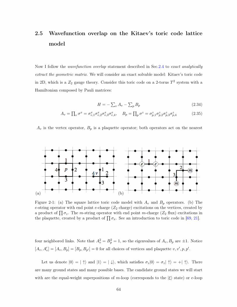
2.5 Wavefunction overlap on the Kitaev’s toric code lattice
model
Now I follow the wavefunction overlap statement described in Sec.2.4 to exact analytically
extract the geometric matrix. We will consider an exact solvable model: Kitaev’s toric code
in 2D, which is a 𝑍2 gauge theory. Consider this toric code on a 2-torus 𝑇 2 system with a
Hamiltonian composed by Pauli matrices:
𝐻 = −∑
𝑣 𝐴𝑣 −∑
𝑝𝐵𝑝 (2.34)
𝐴𝑣 =∏𝑣 𝜎
𝑥 = 𝜎𝑥𝑣,1𝜎𝑥𝑣,2𝜎
𝑥𝑣,3𝜎
𝑥𝑣,4, 𝐵𝑝 =
∏𝑝 𝜎
𝑧 = 𝜎𝑧𝑝,1𝜎𝑧𝑝,2𝜎
𝑧𝑝,3𝜎
𝑧𝑝,4 (2.35)
𝐴𝑣 is the vertex operator, 𝐵𝑝 is a plaquette operator; both operators act on the nearest
(a) (b)
Figure 2-1: (a) The square lattice toric code model with 𝐴𝑣 and 𝐵𝑝 operators. (b) The𝑒-string operator with end point 𝑒-charge (𝑍2 charge) excitations on the vertices, created bya product of
∏𝜎𝑧. The 𝑚-string operator with end point 𝑚-charge (𝑍2 flux) excitations in
the plaquette, created by a product of∏𝜎𝑥. See an introduction to toric code in [69, 21].
four neighbored links. Note that 𝐴2𝑣 = 𝐵2
𝑝 = 1, so the eigenvalues of 𝐴𝑣, 𝐵𝑝 are ±1. Notice
[𝐴𝑣, 𝐴′𝑣] = [𝐴𝑣, 𝐵𝑝] = [𝐵𝑝, 𝐵𝑝′ ] = 0 for all choices of vertices and plaquette 𝑣, 𝑣′, 𝑝, 𝑝′.
Let us denote |0⟩ = | ↑⟩ and |1⟩ = | ↓⟩, which satisfies 𝜎𝑧|0⟩ = 𝜎𝑧| ↑⟩ = +| ↑⟩. There
are many ground states and many possible bases. The candidate ground states we will start
with are the equal-weight superpositions of 𝑚-loop (corresponds to the |𝜉⟩ state) or 𝑒-loop
64
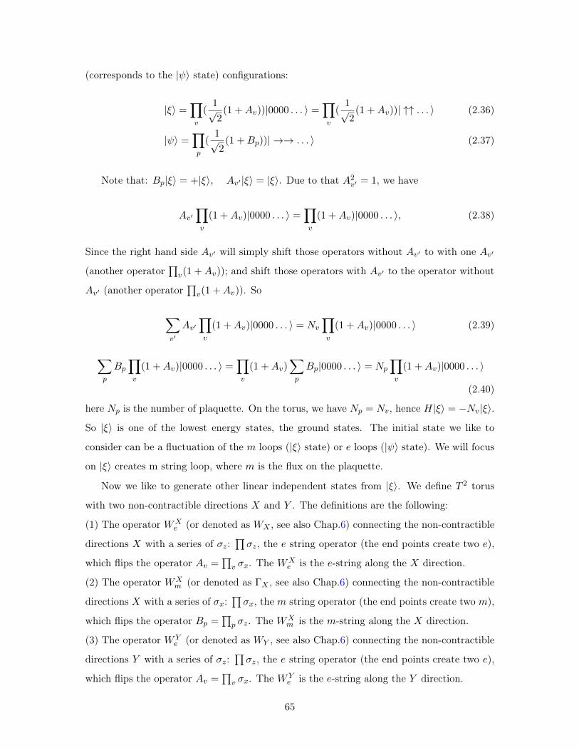
(corresponds to the |𝜓⟩ state) configurations:
|𝜉⟩ =∏𝑣
(1√2(1 +𝐴𝑣))|0000 . . . ⟩ =
∏𝑣
(1√2(1 +𝐴𝑣))| ↑↑ . . . ⟩ (2.36)
|𝜓⟩ =∏𝑝
(1√2(1 +𝐵𝑝))| →→ . . . ⟩ (2.37)
Note that: 𝐵𝑝|𝜉⟩ = +|𝜉⟩, 𝐴𝑣′ |𝜉⟩ = |𝜉⟩. Due to that 𝐴2𝑣′ = 1, we have
𝐴𝑣′∏𝑣
(1 +𝐴𝑣)|0000 . . . ⟩ =∏𝑣
(1 +𝐴𝑣)|0000 . . . ⟩, (2.38)
Since the right hand side 𝐴𝑣′ will simply shift those operators without 𝐴𝑣′ to with one 𝐴𝑣′
(another operator∏𝑣(1 +𝐴𝑣)); and shift those operators with 𝐴𝑣′ to the operator without
𝐴𝑣′ (another operator∏𝑣(1 +𝐴𝑣)). So
∑𝑣′
𝐴𝑣′∏𝑣
(1 +𝐴𝑣)|0000 . . . ⟩ = 𝑁𝑣
∏𝑣
(1 +𝐴𝑣)|0000 . . . ⟩ (2.39)
∑𝑝
𝐵𝑝∏𝑣
(1 +𝐴𝑣)|0000 . . . ⟩ =∏𝑣
(1 +𝐴𝑣)∑𝑝
𝐵𝑝|0000 . . . ⟩ = 𝑁𝑝
∏𝑣
(1 +𝐴𝑣)|0000 . . . ⟩
(2.40)
here 𝑁𝑝 is the number of plaquette. On the torus, we have 𝑁𝑝 = 𝑁𝑣, hence 𝐻|𝜉⟩ = −𝑁𝑣|𝜉⟩.
So |𝜉⟩ is one of the lowest energy states, the ground states. The initial state we like to
consider can be a fluctuation of the 𝑚 loops (|𝜉⟩ state) or 𝑒 loops (|𝜓⟩ state). We will focus
on |𝜉⟩ creates m string loop, where 𝑚 is the flux on the plaquette.
Now we like to generate other linear independent states from |𝜉⟩. We define 𝑇 2 torus
with two non-contractible directions 𝑋 and 𝑌 . The definitions are the following:
(1) The operator 𝑊𝑋𝑒 (or denoted as 𝑊𝑋 , see also Chap.6) connecting the non-contractible
directions 𝑋 with a series of 𝜎𝑧:∏𝜎𝑧, the 𝑒 string operator (the end points create two 𝑒),
which flips the operator 𝐴𝑣 =∏𝑣 𝜎𝑥. The 𝑊𝑋
𝑒 is the 𝑒-string along the 𝑋 direction.
(2) The operator 𝑊𝑋𝑚 (or denoted as Γ𝑋 , see also Chap.6) connecting the non-contractible
directions 𝑋 with a series of 𝜎𝑥:∏𝜎𝑥, the 𝑚 string operator (the end points create two 𝑚),
which flips the operator 𝐵𝑝 =∏𝑝 𝜎𝑧. The 𝑊𝑋
𝑚 is the 𝑚-string along the 𝑋 direction.
(3) The operator 𝑊 𝑌𝑒 (or denoted as 𝑊𝑌 , see also Chap.6) connecting the non-contractible
directions 𝑌 with a series of 𝜎𝑧:∏𝜎𝑧, the 𝑒 string operator (the end points create two 𝑒),
which flips the operator 𝐴𝑣 =∏𝑣 𝜎𝑥. The 𝑊 𝑌
𝑒 is the 𝑒-string along the 𝑌 direction.
65
(4) The operator 𝑊 𝑌𝑚 (or denoted as Γ𝑌 in Chap.6) connecting the non-contractible direc-
tions 𝑌 with a series of 𝜎𝑥:∏𝜎𝑥, the 𝑚 string operator (the end points create two 𝑚),
which flips the operator 𝐵𝑝 =∏𝑝 𝜎𝑧. The 𝑊 𝑌
𝑚 is the 𝑚-string along the 𝑌 direction.
Note that [𝑊𝑋𝑚 ,𝑊
𝑌𝑚 ] = [𝑊𝑋
𝑒 ,𝑊𝑌𝑒 ] = 0. 𝑊𝑋
𝑚𝑊𝑌𝑒 = −𝑊 𝑌
𝑒 𝑊𝑋𝑚 , and𝑊 𝑌
𝑚𝑊𝑋𝑒 = −𝑊𝑋
𝑒 𝑊𝑌𝑚 .
Let us start from the superposition of fluctuating𝑚-loop state of |𝜉⟩ =∏𝑣(
1√2(1+𝐴𝑣))|0000 . . . ⟩.
It is important to note that
𝑊𝑋𝑒 |𝜉⟩ = |𝜉⟩, 𝑊 𝑌
𝑒 |𝜉⟩ = |𝜉⟩ (2.41)
adding a non-contractible 𝑒-loop 𝑊𝑋𝑒 along 𝑥 direction on superposed fluctuating 𝑚-loop
state gives the same state |𝜉⟩. However, adding a non-contractible 𝑚-loop 𝑊𝑋𝑚 on |𝜉⟩
gives different state. We require an even number of 𝜎𝑧, 𝜎𝑥 overlapping on the 𝑊𝑋𝑒 |𝜉⟩ =∏
𝜎𝑧∏𝑣(1 +
∏𝑣 𝜎𝑥)|0000 . . . ⟩ =
∏𝑣(1 +
∏𝑣 𝜎𝑥)
∏𝜎𝑧|0000 . . . ⟩ = |𝜉⟩.
Let us choose 𝑊𝑋𝑒 ,𝑊
𝑋𝑚 operator as the chosen measurements from all the Hilbert space
operators; we wish to simultaneously diagonalize the two operators in the eigenstate basis.
Meanwhile we wish to define the trivial vacuum ground state |I⟩ as the state where there is
only trivial measurement observed by the 𝑊𝑋𝑒 ’s 𝑒 loop and 𝑊𝑋
𝑚 ’s 𝑚 loop along the 𝑥 direc-
tion. Namely, there is no 𝑒 or 𝑚-string non-contractible loop along the 𝑦 direction. The goal
is to find a relation between |I⟩ and |𝜉⟩: |I⟩ =∑𝑐(𝑛1, 𝑛2, 𝑛3, 𝑛4) (𝑊𝑋
𝑚 )𝑛1 (𝑊 𝑌𝑚 )𝑛2(𝑊𝑋
𝑒 )𝑛3
(𝑊 𝑌𝑒 )𝑛4 |𝜉⟩ which satisfies 𝑊𝑋
𝑒 |I⟩ = |I⟩ and 𝑊𝑋𝑚 |I⟩ = |I⟩. It turns out that our |𝜉⟩ as the su-
perposition of the fluctuating 𝑚 loop states is important to determine |I⟩. We will find that
|I⟩ simply be the superposition of the |𝜉⟩ and the state with a non-contractible
𝑚-loop winding around the 𝑥-direction:
|I⟩ = 1√2(|𝜉⟩+𝑊𝑋
𝑚 |𝜉⟩). (2.42)
66

To prove this, define |(𝑎, 𝑏)⟩ = (𝑊𝑋𝑚 )𝑎(𝑊 𝑌
𝑚 )𝑏|𝜉⟩:
𝑊𝑋𝑚 |(𝑎, 𝑏)⟩ = (𝑊𝑋
𝑚 )𝑎+1(𝑊 𝑌𝑚 )𝑏|𝜉⟩ = |(𝑎+ 1, 𝑏)⟩ (2.43)
𝑊 𝑌𝑚 |(𝑎, 𝑏)⟩ = |(𝑎, 𝑏+ 1)⟩ (2.44)
𝑊𝑋𝑒 |(𝑎, 𝑏)⟩ = (−1)𝑏(𝑊𝑋
𝑚 )𝑎+1(𝑊 𝑌𝑚 )𝑏(𝑊𝑋
𝑒 )|𝜉⟩ = (−1)𝑏|(𝑎, 𝑏)⟩ (2.45)
𝑊 𝑌𝑒 |(𝑎, 𝑏)⟩ = (−1)𝑎|(𝑎, 𝑏)⟩ (2.46)
Here 𝑊𝑋𝑒 |𝜉⟩ = |𝜉⟩ is a nontrivial step. We have contractible loop states |𝜉⟩ = Γ(𝜎𝑥)|00 . . . ⟩,
and 𝑊𝑋𝑒 (𝜎𝑧)Γ(𝜎𝑥)|00 . . . ⟩ ∝ Γ(𝜎𝑥)|00 . . . ⟩. This should imply that 𝑊𝑋
𝑒 |𝜉⟩ = 𝑊 𝑌𝑒 |𝜉⟩ = |𝜉⟩
if we have the 𝑚-loop superposed state being acted by 𝑒-non-contractible loop along any
direction on an even lattice site system.
Define: |(±, 𝑏)⟩ ≡ 1√2(|(0, 𝑏)⟩±|(1, 𝑏)⟩) we see that𝑊𝑋
𝑒 |(±, 𝑏)⟩ = (−1)𝑏|(±, 𝑏)⟩,𝑊𝑋𝑚 |(±, 𝑏)⟩
= ±|(±, 𝑏)⟩ so 𝑊𝑋𝑒 |(+, 0)⟩ =𝑊𝑋
𝑚 |(+, 0)⟩ = |(+, 0)⟩.
|I⟩ ≡ |(+, 0)⟩ = 1√2(|𝜉⟩+𝑊𝑋
𝑚 |𝜉⟩) (2.47)
Now, |I⟩ has no non-contractible 𝑒,𝑚 along 𝑦 direction detectible by 𝑊𝑋𝑒 ,𝑊
𝑋𝑚 . So all we
need to do is creating 𝑒 and 𝑚 along 𝑦 direction by 𝑊 𝑌𝑒 for 𝑒 and 𝑊 𝑌
𝑚 for 𝑚.
|I⟩ = 1√2(|(0, 0)⟩+ |(1, 0)⟩) = 1√
2(|𝜉⟩+𝑊𝑋
𝑚 |𝜉⟩) (2.48)
|𝑒⟩ =𝑊 𝑌𝑒 |I⟩ =
1√2(|(0, 0)⟩ − |(1, 0)⟩) = 1√
2(|𝜉⟩ −𝑊𝑋
𝑚 |𝜉⟩) (2.49)
|𝑚⟩ =𝑊 𝑌𝑚 |I⟩ =
1√2(|(0, 1)⟩+ |(1, 1)⟩) = 1√
2(𝑊 𝑌
𝑚 |𝜉⟩+𝑊𝑋𝑚𝑊
𝑌𝑚 |𝜉⟩) (2.50)
|𝑒𝑚⟩ =𝑊 𝑌𝑒 𝑊
𝑌𝑚 |I⟩ =
1√2(|(0, 1)⟩ − |(1, 1)⟩) = 1√
2(𝑊 𝑌
𝑚 |𝜉⟩ −𝑊𝑋𝑚𝑊
𝑌𝑚 |𝜉⟩). (2.51)
Now we can do the modular SL(2,Z) transformation 𝒮 which sends (𝑥, 𝑦)→ (−𝑦, 𝑥).
𝒮|I⟩ = 1√2(|(0, 0)⟩+ |(0, 1)⟩) = 1
2(|I⟩+ |𝑒⟩+ |𝑚⟩+ |𝑒𝑚⟩) (2.52)
𝒮|𝑒⟩ = 1√2(|(0, 0)⟩ − |(0, 1)⟩) = 1
2(|I⟩+ |𝑒⟩ − |𝑚⟩ − |𝑒𝑚⟩) (2.53)
𝒮|𝑚⟩ = 1√2(|(−1, 0)⟩+ |(−1, 1)⟩) = 1
2(|I⟩ − |𝑒⟩+ |𝑚⟩ − |𝑒𝑚⟩) (2.54)
𝒮|𝑒𝑚⟩ = 1√2(|(−1, 0)⟩ − |(−1, 1)⟩) = 1
2(|I⟩ − |𝑒⟩ − |𝑚⟩+ |𝑒𝑚⟩). (2.55)
67
Clearly, we have now obtained the ideal 𝒮 matrix in the ideal quasi-particle basis using the
wave function overlap approach:
𝒮 =
⎛⎜⎜⎜⎜⎜⎜⎝⟨I|𝒮|I⟩ ⟨I|𝒮|𝑒⟩ ⟨I|𝒮|𝑚⟩ ⟨I|𝒮|𝑒𝑚⟩
⟨𝑒|𝒮|I⟩ ⟨𝑒|𝒮|𝑒⟩ ⟨𝑒|𝒮|𝑚⟩ ⟨𝑒|𝒮|𝑒𝑚⟩
⟨𝑚|𝒮|I⟩ ⟨𝑚|𝒮|𝑒⟩ ⟨𝑚|𝒮|𝑚⟩ ⟨𝑚|𝒮|𝑒𝑚⟩
⟨𝑒𝑚|𝒮|I⟩ ⟨𝑒𝑚|𝒮|𝑒⟩ ⟨𝑒𝑚|𝒮|𝑚⟩ ⟨𝑒𝑚|𝒮|𝑒𝑚⟩
⎞⎟⎟⎟⎟⎟⎟⎠ =1
2
⎛⎜⎜⎜⎜⎜⎜⎝1 1 1 1
1 1 −1 −1
1 −1 1 −1
1 −1 −1 1
⎞⎟⎟⎟⎟⎟⎟⎠ . (2.56)
This can also be obtained as minimal entangled states (MES), through another approach
by entanglement entropy [85].
Comparison: The final comment is that the adiabatic Berry phase / geometric
matrix calculation has the drawbacks of requiring tuning Hamiltonian coupling constants
thus demanding to access a large class of systems; but it has the advantages of dealing
with non-translational-symmetry, non-periodic and non-lattice system. On the other hand,
the wavefunction overlap has advantages of fixing a single Hamiltonian with different
degenerate ground states; but it has the drawbacks of restricting to translational-symmetry,
periodic and equal-size-lattice system and to the given symmetry of lattice systems (usually
easier to extract 𝒮 but harder to extract 𝒯 ) [85]. There is also a drawback that in general
there is a volume-dependent factor ⟨𝜓𝛼|��|𝜓𝛽⟩ = e−#𝑉 · 𝑂𝛼,𝛽 · . . . , although in our square-
lattice toric code example, we did not observe the volume-dependent term in 𝒮, but it indeed
occurs in 𝒯 , at least for square and triangle lattice studied in [83].
2.6 Spacetime path integral approach for the modular 𝒮 and
𝒯 in 2+1D and 3+1D: group cohomology cocycle
Below we will describe the spacetime path integral approach with discretized lattice trian-
gulation of spacetime. There are two versions, one is for topological order where degrees
of freedom live on the links (Sec.2.6.1) while gauge theory summing over all possible gauge
configurations, the other is SPTs where degrees of freedom live on the sites (Sec.2.6.2). In
short, on any closed manifold, the former has |ZTO| ≥ 1, but the former is restricted to
|ZSPT| = 1.
68
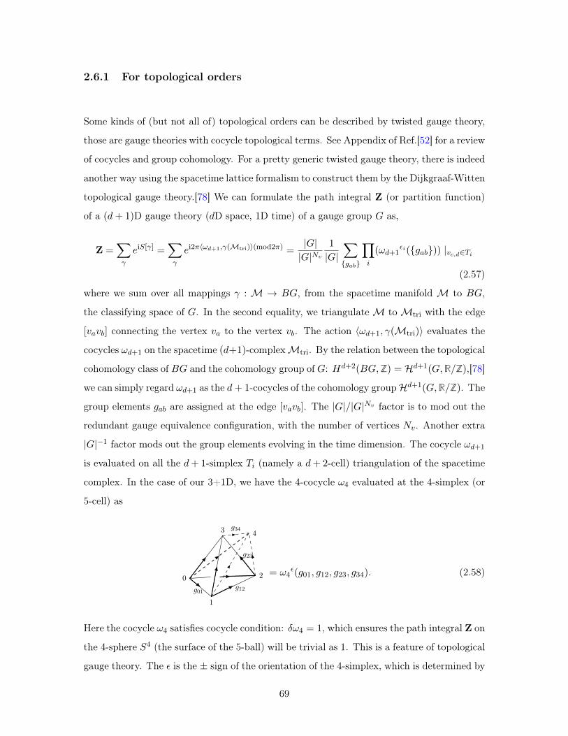
2.6.1 For topological orders
Some kinds of (but not all of) topological orders can be described by twisted gauge theory,
those are gauge theories with cocycle topological terms. See Appendix of Ref.[52] for a review
of cocycles and group cohomology. For a pretty generic twisted gauge theory, there is indeed
another way using the spacetime lattice formalism to construct them by the Dijkgraaf-Witten
topological gauge theory.[78] We can formulate the path integral Z (or partition function)
of a (𝑑+ 1)D gauge theory (𝑑D space, 1D time) of a gauge group 𝐺 as,
Z =∑𝛾
𝑒i𝑆[𝛾] =∑𝛾
𝑒i2𝜋⟨𝜔𝑑+1,𝛾(ℳtri)⟩(mod2𝜋) =|𝐺||𝐺|𝑁𝑣
1
|𝐺|∑{𝑔𝑎𝑏}
∏𝑖
(𝜔𝑑+1𝜖𝑖({𝑔𝑎𝑏})) |𝑣𝑐,𝑑∈𝑇𝑖
(2.57)
where we sum over all mappings 𝛾 : ℳ → 𝐵𝐺, from the spacetime manifold ℳ to 𝐵𝐺,
the classifying space of 𝐺. In the second equality, we triangulate ℳ to ℳtri with the edge
[𝑣𝑎𝑣𝑏] connecting the vertex 𝑣𝑎 to the vertex 𝑣𝑏. The action ⟨𝜔𝑑+1, 𝛾(ℳtri)⟩ evaluates the
cocycles 𝜔𝑑+1 on the spacetime (𝑑+1)-complexℳtri. By the relation between the topological
cohomology class of 𝐵𝐺 and the cohomology group of 𝐺: 𝐻𝑑+2(𝐵𝐺,Z) = ℋ𝑑+1(𝐺,R/Z),[78]
we can simply regard 𝜔𝑑+1 as the 𝑑+ 1-cocycles of the cohomology groupℋ𝑑+1(𝐺,R/Z). The
group elements 𝑔𝑎𝑏 are assigned at the edge [𝑣𝑎𝑣𝑏]. The |𝐺|/|𝐺|𝑁𝑣 factor is to mod out the
redundant gauge equivalence configuration, with the number of vertices 𝑁𝑣. Another extra
|𝐺|−1 factor mods out the group elements evolving in the time dimension. The cocycle 𝜔𝑑+1
is evaluated on all the 𝑑+ 1-simplex 𝑇𝑖 (namely a 𝑑+ 2-cell) triangulation of the spacetime
complex. In the case of our 3+1D, we have the 4-cocycle 𝜔4 evaluated at the 4-simplex (or
5-cell) as
0
1
2
3 4
𝑔01 𝑔12
𝑔23
𝑔34
= 𝜔4𝜖(𝑔01, 𝑔12, 𝑔23, 𝑔34). (2.58)
Here the cocycle 𝜔4 satisfies cocycle condition: 𝛿𝜔4 = 1, which ensures the path integral Z on
the 4-sphere 𝑆4 (the surface of the 5-ball) will be trivial as 1. This is a feature of topological
gauge theory. The 𝜖 is the ± sign of the orientation of the 4-simplex, which is determined by
69
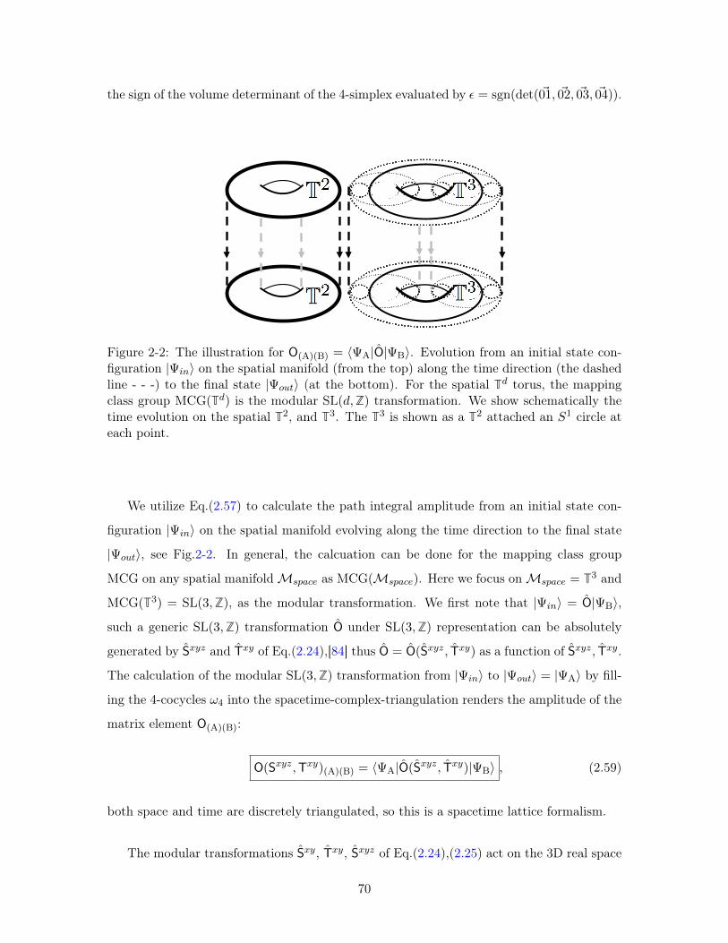
the sign of the volume determinant of the 4-simplex evaluated by 𝜖 = sgn(det(01, 02, 03, 04)).
Figure 2-2: The illustration for O(A)(B) = ⟨ΨA|O|ΨB⟩. Evolution from an initial state con-figuration |Ψ𝑖𝑛⟩ on the spatial manifold (from the top) along the time direction (the dashedline - - -) to the final state |Ψ𝑜𝑢𝑡⟩ (at the bottom). For the spatial T𝑑 torus, the mappingclass group MCG(T𝑑) is the modular SL(𝑑,Z) transformation. We show schematically thetime evolution on the spatial T2, and T3. The T3 is shown as a T2 attached an 𝑆1 circle ateach point.
We utilize Eq.(2.57) to calculate the path integral amplitude from an initial state con-
figuration |Ψ𝑖𝑛⟩ on the spatial manifold evolving along the time direction to the final state
|Ψ𝑜𝑢𝑡⟩, see Fig.2-2. In general, the calcuation can be done for the mapping class group
MCG on any spatial manifoldℳ𝑠𝑝𝑎𝑐𝑒 as MCG(ℳ𝑠𝑝𝑎𝑐𝑒). Here we focus onℳ𝑠𝑝𝑎𝑐𝑒 = T3 and
MCG(T3) = SL(3,Z), as the modular transformation. We first note that |Ψ𝑖𝑛⟩ = O|ΨB⟩,
such a generic SL(3,Z) transformation O under SL(3,Z) representation can be absolutely
generated by S𝑥𝑦𝑧 and T𝑥𝑦 of Eq.(2.24),[84] thus O = O(S𝑥𝑦𝑧, T𝑥𝑦) as a function of S𝑥𝑦𝑧, T𝑥𝑦.
The calculation of the modular SL(3,Z) transformation from |Ψ𝑖𝑛⟩ to |Ψ𝑜𝑢𝑡⟩ = |ΨA⟩ by fill-
ing the 4-cocycles 𝜔4 into the spacetime-complex-triangulation renders the amplitude of the
matrix element O(A)(B):
O(S𝑥𝑦𝑧,T𝑥𝑦)(A)(B) = ⟨ΨA|O(S𝑥𝑦𝑧, T𝑥𝑦)|ΨB⟩ , (2.59)
both space and time are discretely triangulated, so this is a spacetime lattice formalism.
The modular transformations S𝑥𝑦, T𝑥𝑦, S𝑥𝑦𝑧 of Eq.(2.24),(2.25) act on the 3D real space
70
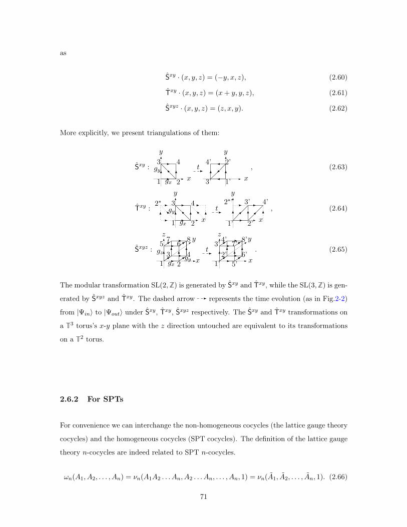
as
S𝑥𝑦 · (𝑥, 𝑦, 𝑧) = (−𝑦, 𝑥, 𝑧), (2.60)
T𝑥𝑦 · (𝑥, 𝑦, 𝑧) = (𝑥+ 𝑦, 𝑦, 𝑧), (2.61)
S𝑥𝑦𝑧 · (𝑥, 𝑦, 𝑧) = (𝑧, 𝑥, 𝑦). (2.62)
More explicitly, we present triangulations of them:
S𝑥𝑦 :
1
3
2
4
𝑥
𝑦
𝑔𝑥
𝑔𝑦 𝑡
1’3’
2’4’
𝑥
𝑦
, (2.63)
T𝑥𝑦 :
1
3
2
42*
𝑥
𝑦
𝑔𝑥
𝑔𝑦 𝑡
1’
3’
2’
4’2*’
𝑥
𝑦
, (2.64)
S𝑥𝑦𝑧 :
1
5
23 4
67 8
𝑥
𝑦𝑧
𝑔𝑥𝑔𝑦
𝑔𝑧 𝑡
1’
3’
5’2’ 6’
7’4’ 8’
𝑥
𝑦𝑧
. (2.65)
The modular transformation SL(2,Z) is generated by S𝑥𝑦 and T𝑥𝑦, while the SL(3,Z) is gen-
erated by S𝑥𝑦𝑧 and T𝑥𝑦. The dashed arrow represents the time evolution (as in Fig.2-2)
from |Ψ𝑖𝑛⟩ to |Ψ𝑜𝑢𝑡⟩ under S𝑥𝑦, T𝑥𝑦, S𝑥𝑦𝑧 respectively. The S𝑥𝑦 and T𝑥𝑦 transformations on
a T3 torus’s 𝑥-𝑦 plane with the 𝑧 direction untouched are equivalent to its transformations
on a T2 torus.
2.6.2 For SPTs
For convenience we can interchange the non-homogeneous cocycles (the lattice gauge theory
cocycles) and the homogeneous cocycles (SPT cocycles). The definition of the lattice gauge
theory 𝑛-cocycles are indeed related to SPT 𝑛-cocycles.
𝜔𝑛(𝐴1, 𝐴2, . . . , 𝐴𝑛) = 𝜈𝑛(𝐴1𝐴2 . . . 𝐴𝑛, 𝐴2 . . . 𝐴𝑛, . . . , 𝐴𝑛, 1) = 𝜈𝑛(𝐴1, 𝐴2, . . . , 𝐴𝑛, 1). (2.66)
71
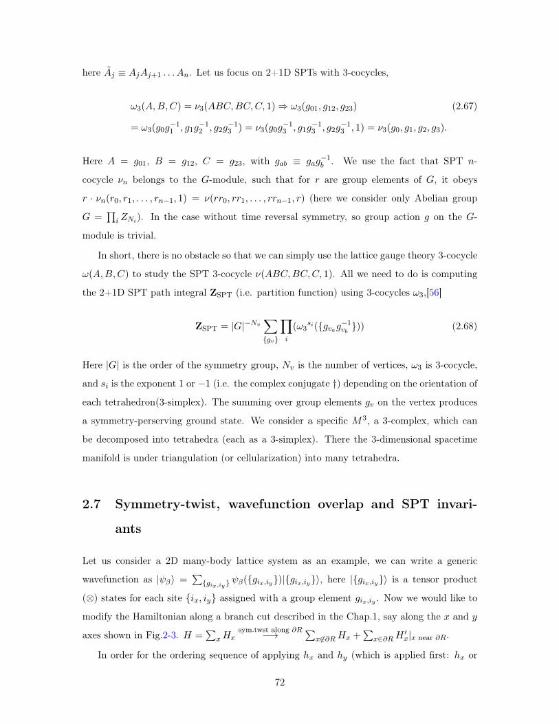
here 𝐴𝑗 ≡ 𝐴𝑗𝐴𝑗+1 . . . 𝐴𝑛. Let us focus on 2+1D SPTs with 3-cocycles,
𝜔3(𝐴,𝐵,𝐶) = 𝜈3(𝐴𝐵𝐶,𝐵𝐶,𝐶, 1)⇒ 𝜔3(𝑔01, 𝑔12, 𝑔23) (2.67)
= 𝜔3(𝑔0𝑔−11 , 𝑔1𝑔
−12 , 𝑔2𝑔
−13 ) = 𝜈3(𝑔0𝑔
−13 , 𝑔1𝑔
−13 , 𝑔2𝑔
−13 , 1) = 𝜈3(𝑔0, 𝑔1, 𝑔2, 𝑔3).
Here 𝐴 = 𝑔01, 𝐵 = 𝑔12, 𝐶 = 𝑔23, with 𝑔𝑎𝑏 ≡ 𝑔𝑎𝑔−1𝑏 . We use the fact that SPT 𝑛-
cocycle 𝜈𝑛 belongs to the 𝐺-module, such that for 𝑟 are group elements of 𝐺, it obeys
𝑟 · 𝜈𝑛(𝑟0, 𝑟1, . . . , 𝑟𝑛−1, 1) = 𝜈(𝑟𝑟0, 𝑟𝑟1, . . . , 𝑟𝑟𝑛−1, 𝑟) (here we consider only Abelian group
𝐺 =∏𝑖 𝑍𝑁𝑖). In the case without time reversal symmetry, so group action 𝑔 on the 𝐺-
module is trivial.
In short, there is no obstacle so that we can simply use the lattice gauge theory 3-cocycle
𝜔(𝐴,𝐵,𝐶) to study the SPT 3-cocycle 𝜈(𝐴𝐵𝐶,𝐵𝐶,𝐶, 1). All we need to do is computing
the 2+1D SPT path integral ZSPT (i.e. partition function) using 3-cocycles 𝜔3,[56]
ZSPT = |𝐺|−𝑁𝑣∑{𝑔𝑣}
∏𝑖
(𝜔3𝑠𝑖({𝑔𝑣𝑎𝑔−1
𝑣𝑏})) (2.68)
Here |𝐺| is the order of the symmetry group, 𝑁𝑣 is the number of vertices, 𝜔3 is 3-cocycle,
and 𝑠𝑖 is the exponent 1 or −1 (i.e. the complex conjugate †) depending on the orientation of
each tetrahedron(3-simplex). The summing over group elements 𝑔𝑣 on the vertex produces
a symmetry-perserving ground state. We consider a specific 𝑀3, a 3-complex, which can
be decomposed into tetrahedra (each as a 3-simplex). There the 3-dimensional spacetime
manifold is under triangulation (or cellularization) into many tetrahedra.
2.7 Symmetry-twist, wavefunction overlap and SPT invari-
ants
Let us consider a 2D many-body lattice system as an example, we can write a generic
wavefunction as |𝜓𝛽⟩ =∑
{𝑔𝑖𝑥,𝑖𝑦} 𝜓𝛽({𝑔𝑖𝑥,𝑖𝑦})|{𝑔𝑖𝑥,𝑖𝑦}⟩, here |{𝑔𝑖𝑥,𝑖𝑦}⟩ is a tensor product
(⊗) states for each site {𝑖𝑥, 𝑖𝑦} assigned with a group element 𝑔𝑖𝑥,𝑖𝑦 . Now we would like to
modify the Hamiltonian along a branch cut described in the Chap.1, say along the 𝑥 and 𝑦
axes shown in Fig.2-3. 𝐻 =∑
𝑥𝐻𝑥sym.twst along 𝜕𝑅−→
∑𝑥 ∈𝜕𝑅𝐻𝑥 +
∑𝑥∈𝜕𝑅𝐻
′𝑥|𝑥 near 𝜕𝑅.
In order for the ordering sequence of applying ℎ𝑥 and ℎ𝑦 (which is applied first: ℎ𝑥 or
72
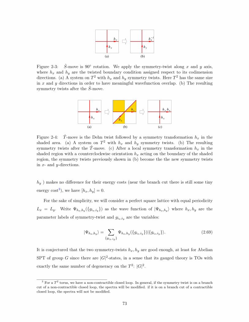
(a) (b)
h
h
x
y
h
h
y
x−1
Figure 2-3: 𝑆-move is 90∘ rotation. We apply the symmetry-twist along 𝑥 and 𝑦 axis,where ℎ𝑥 and ℎ𝑦 are the twisted boundary condition assigned respect to its codimensiondirections. (a) A system on 𝑇 2 with ℎ𝑥 and ℎ𝑦 symmetry twists. Here 𝑇 2 has the same sizein 𝑥 and 𝑦 directions in order to have meaningful wavefunction overlap. (b) The resultingsymmetry twists after the 𝑆-move.
h
h
x
y h y
h x
(a) (b)
h x
(c)
h y h x
Figure 2-4: 𝑇 -move is the Dehn twist followed by a symmetry transformation ℎ𝑥 in theshaded area. (a) A system on 𝑇 2 with ℎ𝑥 and ℎ𝑦 symmetry twists. (b) The resultingsymmetry twists after the 𝑇 -move. (c) After a local symmetry transformation ℎ𝑥 in theshaded region with a counterclockwise orientation ℎ𝑥 acting on the boundary of the shadedregion, the symmetry twists previously shown in (b) become the the new symmetry twistsin 𝑥- and 𝑦-directions.
ℎ𝑦 ) makes no difference for their energy costs (near the branch cut there is still some tiny
energy cost3), we have [ℎ𝑥, ℎ𝑦] = 0.
For the sake of simplicity, we will consider a perfect square lattice with equal periodicity
𝐿𝑥 = 𝐿𝑦. Write Ψℎ𝑥,ℎ𝑦({𝑔𝑖𝑥,𝑖𝑦}) as the wave function of |Ψℎ𝑥,ℎ𝑦⟩ where ℎ𝑥, ℎ𝑦 are the
parameter labels of symmetry-twist and 𝑔𝑖𝑥,𝑖𝑦 are the variables:
|Ψℎ𝑥,ℎ𝑦⟩ =∑
{𝑔𝑖𝑥,𝑖𝑦}
Ψℎ𝑥,ℎ𝑦({𝑔𝑖𝑥,𝑖𝑦})|{𝑔𝑖𝑥,𝑖𝑦}⟩. (2.69)
It is conjectured that the two symmetry-twists ℎ𝑥, ℎ𝑦 are good enough, at least for Abelian
SPT of group 𝐺 since there are |𝐺|2-states, in a sense that its gauged theory is TOs with
exactly the same number of degeneracy on the 𝑇 2: |𝐺|2.
3 For a 𝑇 2 torus, we have a non-contractible closed loop. In general, if the symmetry twist is on a branchcut of a non-contractible closed loop, the spectra will be modified. if it is on a branch cut of a contractibleclosed loop, the spectra will not be modified.
73

Naively, we may guess the wavefunction overlap for SL(2,Z) transformation are:
⟨𝜓𝛼|S|𝜓𝛽⟩?=
∑{𝑔𝑖𝑥,𝑖𝑦}
𝜓*𝛼({𝑔𝑖𝑥,𝑖𝑦})𝜓𝛽({𝑔𝑖−1
𝑦 ,𝑖𝑥}), ⟨𝜓𝛼|T|𝜓𝛽⟩
?=
∑{𝑔},𝑖𝑥,𝑖𝑦
𝜓*𝛼({𝑔𝑖𝑥,𝑖𝑦})𝜓𝛽({𝑔𝑖𝑥+𝑖𝑦 ,𝑖𝑦}).
(2.70)
However, this form is close to the answer, but not entirely correct. Here 𝛼 and 𝛽 should
specify the data of symmetry twists. Moreover, because of the SL(2,Z) transformation on
the spatial 𝑇 2 torus, the symmetry twists 𝛼 and 𝛽 should also be constrained and related.
The symmetry twists 𝛼 and 𝛽 should be the same symmetry twists after taking into account
the SL(2,Z) transformation. This means that we will overlap two wavefunctions in the same
family of Hamiltonian, both twisted by the same symmetry-twist.
The state |Ψℎ𝑥,ℎ𝑦⟩ changes under the modular transformation. Let us define
|Ψ𝑆ℎ𝑥,ℎ𝑦⟩ =
∑{𝑔𝑖𝑥,𝑖𝑦}
Ψℎ𝑥,ℎ𝑦({𝑔−𝑖𝑦 ,𝑖𝑥})|{𝑔𝑖𝑥,𝑖𝑦}⟩ =∑
{𝑔𝑖𝑥,𝑖𝑦}
Ψℎ𝑥,ℎ𝑦({𝑔𝑆·(𝑖𝑥,𝑖𝑦)})|{𝑔𝑖𝑥,𝑖𝑦}⟩,
|Ψ𝑇ℎ𝑥,ℎ𝑦⟩ =
∑{𝑔𝑖𝑥,𝑖𝑦}
Ψℎ𝑥,ℎ𝑦({𝑔𝑖𝑥+𝑖𝑦 ,𝑖𝑦})|{𝑔𝑖𝑥,𝑖𝑦}⟩ =∑
{𝑔𝑖𝑥,𝑖𝑦}
Ψℎ𝑥,ℎ𝑦({𝑔𝑇 ·(𝑖𝑥,𝑖𝑦)})|{𝑔𝑖𝑥,𝑖𝑦}⟩. (2.71)
We note that the state |Ψ𝑆ℎ𝑥,ℎ𝑦⟩ and the state |Ψℎ′𝑥,ℎ
′𝑦⟩ have the same symmetry twists if
(ℎ′𝑥, ℎ′𝑦) = (ℎ−1
𝑦 , ℎ𝑥). Thus we can define a matrix
𝑆(ℎ′𝑥,ℎ′𝑦),(ℎ𝑥,ℎ𝑦) = 𝛿ℎ′𝑥,ℎ−1𝑦𝛿ℎ′𝑦 ,ℎ𝑥⟨Ψℎ′𝑥,ℎ
′𝑦|Ψ𝑆
ℎ𝑥,ℎ𝑦⟩ = 𝛿(ℎ′𝑥,ℎ′𝑦),𝑆·(ℎ𝑥,ℎ𝑦)⟨Ψℎ′𝑥,ℎ
′𝑦|Ψ𝑆
ℎ𝑥,ℎ𝑦⟩. (2.72)
However, |Ψ𝑇ℎ𝑥,ℎ𝑦⟩ and |Ψℎ′𝑥,ℎ
′𝑦⟩ always have different branch cuts of the symmetry twists (see
Fig. 2-4(b)). To make their symmetry twists comparable, we perform an additional local
symmetry transformation ℎ𝑥 in the shaded region Fig. 2-4(b), which changes |Ψ𝑇ℎ𝑥,ℎ𝑦⟩ to
|Ψ𝑇ℎ𝑥,ℎ𝑦⟩. Now |Ψ𝑇
ℎ𝑥,ℎ𝑦⟩ and |Ψℎ′𝑥,ℎ
′𝑦⟩ have the same symmetry twists if (ℎ′𝑥, ℎ′𝑦) = (ℎ𝑥, ℎ𝑦ℎ𝑥)
(see Fig. 2-4(c)). Thus we define a matrix
𝑇(ℎ′𝑥,ℎ′𝑦),(ℎ𝑥,ℎ𝑦) = 𝛿ℎ′𝑥,ℎ𝑥ℎ𝑦𝛿ℎ′𝑦 ,ℎ𝑥⟨Ψℎ′𝑥,ℎ′𝑦|Ψ𝑇
ℎ𝑥,ℎ𝑦⟩ = 𝛿(ℎ′𝑥,ℎ′𝑦),𝑇 ·(ℎ𝑥,ℎ𝑦)⟨Ψℎ′𝑥,ℎ
′𝑦|Ψ𝑇
ℎ𝑥,ℎ𝑦⟩. (2.73)
There is an additional operation called group actions ��(𝑔), which sends group ele-
ments to other elements in conjugacy class: ℎ → 𝑔ℎ𝑔−1. In general, ��(𝑔)|Ψ(ℎ𝑥,ℎ𝑦)⟩ =
𝑈(𝑔ℎ𝑥𝑔−1,𝑔ℎ𝑦𝑔−1),(ℎ𝑥,ℎ𝑦)|Ψ𝑔ℎ𝑥𝑔−1,𝑔ℎ𝑦𝑔−1⟩. The factor 𝑈ℎ𝑥,ℎ𝑦(𝑔) is a U(1) phase occurs when
74

evolving |Ψ(ℎ𝑥,ℎ𝑦)⟩ to |Ψ𝑔ℎ𝑥𝑔−1,𝑔ℎ𝑦𝑔−1⟩ state. The nontrivial geometric matrix element is:
��(𝑔)(ℎ′𝑥,ℎ′𝑦),(ℎ𝑥,ℎ𝑦) = 𝛿ℎ′𝑥,𝑔ℎ𝑥𝑔−1𝛿ℎ′𝑦 ,𝑔ℎ𝑦𝑔−1⟨Ψ(𝑔ℎ𝑥𝑔−1,𝑔ℎ𝑦𝑔−1)|��(𝑔)|Ψ(ℎ𝑥,ℎ𝑦)⟩
= 𝛿ℎ′𝑥,𝑔ℎ𝑥𝑔−1𝛿ℎ′𝑦 ,𝑔ℎ𝑦𝑔−1𝑈ℎ𝑥,ℎ𝑦(𝑔). (2.74)
More generally, for any combination of SL(2,Z) transformation, we find that 4
��(ℎ′𝑥,ℎ′𝑦),(ℎ𝑥,ℎ𝑦)
= 𝛿(ℎ′𝑥,ℎ′𝑦),𝜎𝑥·��𝑡·𝜎𝑥·(ℎ𝑥,ℎ𝑦)⟨Ψℎ′𝑥,ℎ′𝑦|Ψ𝑂
ℎ𝑥,ℎ𝑦⟩ , (2.75)
here |Ψ𝑂ℎ𝑥,ℎ𝑦⟩ is obtained from
∑{𝑔𝑖𝑥,𝑖𝑦}Ψℎ𝑥,ℎ𝑦({𝑔��·(𝑖𝑥,𝑖𝑦)})|{𝑔𝑖𝑥,𝑖𝑦}⟩ subject to an additional
change on a shaded area in order to have the same branch-cut configuration as |Ψℎ𝑥,ℎ𝑦⟩.
In general, there are an area dependent factor with non-universal constants 𝑐𝑆 , 𝑐𝑇 :
𝑆(ℎ′𝑥,ℎ′𝑦),(ℎ𝑥,ℎ𝑦) = e−𝑐𝑆𝐿2+𝑜(1/𝐿)𝛿(ℎ′𝑥,ℎ′𝑦),𝑆·(ℎ𝑥,ℎ𝑦)
𝒮(ℎ𝑥,ℎ𝑦),
𝑇(ℎ′𝑥,ℎ′𝑦),(ℎ𝑥,ℎ𝑦) = e−𝑐𝑇𝐿2+𝑜(1/𝐿)𝛿(ℎ′𝑥,ℎ′𝑦),𝑇 ·(ℎ𝑥,ℎ𝑦)
𝒯(ℎ𝑥,ℎ𝑦),
��(𝑔)(ℎ′𝑥,ℎ′𝑦),(ℎ𝑥,ℎ𝑦) = 𝛿ℎ′𝑥,𝑔ℎ𝑥𝑔−1𝛿ℎ′𝑦 ,𝑔ℎ𝑦𝑔−1𝑈ℎ𝑥,ℎ𝑦(𝑔). (2.76)
Importantly the 𝑈 move has no additional volume-dependent factor because it is a group
action which does not deform through any diffeomorphism or MCG elements. Our goal
is to extract the geometric matrix: 𝒮(ℎ𝑥,ℎ𝑦), 𝒯(ℎ𝑥,ℎ𝑦), 𝑈ℎ𝑥,ℎ𝑦(𝑔). However, such geometric
matrices are not yet universal enough. When (ℎ′𝑥, ℎ′𝑦) = (ℎ𝑥, ℎ𝑦), the complex phases
𝑆ℎ𝑥,ℎ𝑦 , 𝑇ℎ𝑥,ℎ𝑦 , 𝑈ℎ𝑥,ℎ𝑦(ℎ𝑡) are not well defined, since they depend on the choices of the phases
of |Ψ(ℎ𝑥,ℎ𝑦)⟩ and |Ψ(ℎ′𝑥,ℎ′𝑦)⟩. To obtain the universal geometric matrix, we need to send
|Ψ(ℎ𝑥,ℎ𝑦)⟩ back to |Ψ(ℎ𝑥,ℎ𝑦)⟩— the product of 𝑆ℎ𝑥,ℎ𝑦 , 𝑇ℎ𝑥,ℎ𝑦 , 𝑈ℎ𝑥,ℎ𝑦(ℎ𝑡) around a closed orbit
(ℎ𝑥, ℎ𝑦) → (ℎ′𝑥, ℎ′𝑦) → · · · → (ℎ𝑥, ℎ𝑦) is universal (see Fig. 2-5). We believe that those
products for various closed orbits completely characterize the 2+1D SPTs. The same idea
applies to SPTs in any dimension.
4Here 𝜎𝑥 ·��𝑡 ·𝜎𝑥 ·(ℎ𝑥, ℎ𝑦) is defined as(0 11 0
)��𝑡
(0 11 0
)( ℎ𝑥ℎ𝑦
). In particular, 𝜎𝑥 ·𝑆𝑡 ·𝜎𝑥 = 𝑆 and 𝜎𝑥 ·𝑇 𝑡 ·𝜎𝑥 = 𝑇 .
It is checked by considering the invariant inner product form (ℎ𝑦, ℎ𝑥) · (��, 𝑦) = (ℎ′𝑦, ℎ
′𝑥) · (𝑥′, 𝑦′)
75
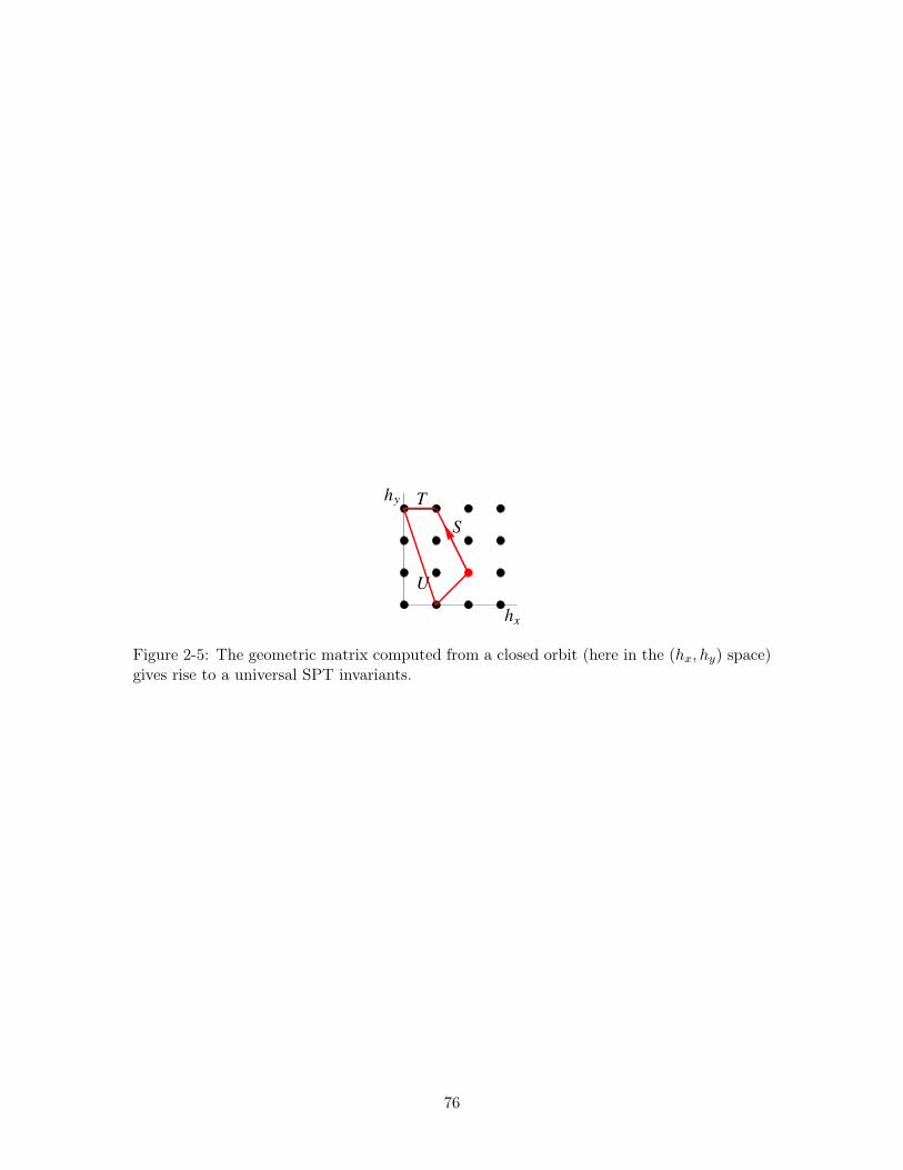
hy
hx
S
T
U
Figure 2-5: The geometric matrix computed from a closed orbit (here in the (ℎ𝑥, ℎ𝑦) space)gives rise to a universal SPT invariants.
76
Chapter 3
Aspects of Symmetry
In Sec.3.1, we extend the idea of symmetry-twist as a similar way of gauging and a way
to couple to external probed field, therefore we can develop an effective probed field action
and partition functions for SPT. In Sec.3.2, we express SPT invariants in terms of physical
observables such as fractional quantum numbers and degenerate zero modes.
3.1 Field theory representation of gauge-gravity SPT invari-
ants, group cohomology and beyond: Probed fields
Gapped systems without symmetry breaking[9, 86] can have intrinsic topological order.
However, even without symmetry breaking and without topological order, gapped systems
can still be nontrivial if there is certain global symmetry protection, known as Symmetry-
Protected Topological states (SPTs). Their non-trivialness can be found in the gapless /
topological boundary modes protected by a global symmetry, which shows gauge or grav-
itational anomalies.[49, 87, 56, 88, 89, 90, 50, 91, 92, 51] More precisely, they are short-
range entangled states which can be deformed to a trivial product state by local unitary
transformation[93, 94] if the deformation breaks the global symmetry. Examples of SPTs
are Haldane spin-1 chain protected by spin rotational symmetry[34, 35] and the topological
insulators protected by fermion number conservation and time reversal symmetry.
While some classes of topological orders can be described by topological quantum field
theories (TQFT),[26, 25] it is less clear how to systematically construct field theory with a
global symmetry to classify or characterize SPTs for any dimension. This challenge origi-
77
nates from the fact that SPTs is naturally defined on a discretized spatial lattice or on a
discretized spacetime path integral by a group cohomology construction[12, 78] instead of
continuous fields. Group cohomology construction of SPTs also reveals a duality between
some SPTs and the Dijkgraaf-Witten topological gauge theory.[78, 95]
Some important progresses have been recently made to tackle the above question. For
example, there are 2+1D Chern-Simons theory, non-linear sigma models, and an orbifolding
approach implementing modular invariance on 1D edge modes. The above approaches have
their own benefits, but they may be either limited to certain dimensions, or be limited to
some special cases. Thus, the previous works may not fulfill all SPTs predicted from group
cohomology classifications.
In this work, we will provide a more systematic way to tackle this problem, by construct-
ing topological response field theory and topological invariants for SPTs (SPT invariants) in
any dimension protected by a symmetry group 𝐺. The new ingredient of our work suggests a
one-to-one correspondence between the continuous semi-classical probe-field partition func-
tion and the discretized cocycle of cohomology group, ℋ𝑑+1(𝐺,R/Z), predicted to classify
𝑑 + 1D SPTs with a symmetry group 𝐺. Moreover, our formalism can even attain SPTs
beyond group cohomology classifications.[91, 92]
3.1.1 Partition function and SPT invariants
For systems that realize topological orders, we can adiabatically deform the ground state
|Ψ𝑔.𝑠.(𝑔)⟩ of parameters 𝑔 via:
⟨Ψ𝑔.𝑠.(𝑔 + 𝛿𝑔)|Ψ𝑔.𝑠.(𝑔)⟩ ≃ . . .Z0 . . . (3.1)
to detect the volume-independent universal piece of partition function, Z0, which reveals
non-Abelian geometric phase of ground states. For systems that realize SPTs, however,
their fixed-point partition functions Z0 always equal to 1 due to its unique ground state on
any closed topology. We cannot distinguish SPTs via Z0. However, due to the existence of
a global symmetry, we can use Z0 with the symmetry twist To define the symmetry twist,
we note that the Hamiltonian 𝐻 =∑
𝑥𝐻𝑥 is invariant under the global symmetry transfor-
mation 𝑈 =∏
all sites 𝑈𝑥, namely 𝐻 = 𝑈𝐻𝑈−1. If we perform the symmetry transformation
𝑈 ′ =∏𝑥∈𝜕𝑅 𝑈𝑥 only near the boundary of a region 𝑅 (say on one side of 𝜕𝑅), the local term
78
𝐻𝑥 of 𝐻 will be modified: 𝐻𝑥 → 𝐻 ′𝑥|𝑥 near 𝜕𝑅. Such a change along a codimension-1 surface
is called a symmetry twist, see Fig.3-1(a)(d), which modifies Z0 to Z0(sym.twist). Just
like the geometric phases of the degenerate ground states characterize topological orders,
we believe that Z0(sym.twist), on different spacetime manifolds and for different symmetry
twists, fully characterizes SPTs.
The symmetry twist is similar to gauging the on-site symmetry[95] except that the
symmetry twist is non-dynamical. We can use the gauge connection 1-form 𝐴 to describe
the corresponding symmetry twists, with probe-fields 𝐴 coupling to the matter fields of the
system. So we can write
Z0(sym.twist) = eiS0(sym.twist) = eiS0(𝐴). (3.2)
Here S0(𝐴) is the SPT invariant that we search for. Eq.(3.2) is a partition function of
classical probe fields, or a topological response theory, obtained by integrating out the
matter fields of SPTs path integral. Below we would like to construct possible forms of
S0(𝐴) based on the following principles: (1) S0(𝐴) is independent of spacetime metrics (i.e.
topological), (2) S0(𝐴) is gauge invariant (for both large and small gauge transformations),
and (3) “Almost flat” connection for probe fields.
U(1) SPTs– Let us start with a simple example of a single global U(1) symmetry. We
can probe the system by coupling the charge fields to an external probe 1-form field 𝐴
(with a U(1) gauge symmetry), and integrate out the matter fields. In 1+1D, we can
write down a partition function by dimensional counting: Z0(sym.twist) = exp[ i 𝜃2𝜋
∫𝐹 ]
with 𝐹 ≡ d𝐴, this is the only term allowed by U(1) gauge symmetry 𝑈 †(𝐴 − id)𝑈 ≃
𝐴 + d𝑓 with 𝑈 = ei𝑓 . More generally, for an even (𝑑 + 1)D spacetime, Z0(sym.twist) =
exp[ i 𝜃
( 𝑑+12
)!(2𝜋)𝑑+12
∫𝐹 ∧ 𝐹 ∧ . . .]. Note that 𝜃 in such an action has no level-quantization
(𝜃 can be an arbitrary real number). Thus this theory does not really correspond to any
nontrivial class, because any 𝜃 is smoothly connected to 𝜃 = 0 which represents a trivial
SPTs.
In an odd dimensional spacetime, such as 2+1D, we have Chern-Simons coupling for
the probe field action Z0(sym.twist) = exp[ i 𝑘4𝜋
∫𝐴 ∧ d𝐴]. More generally, for an odd
(𝑑+1)D, Z0(sym.twist) = exp[ i 2𝜋𝑘( 𝑑+2
2)!(2𝜋)(𝑑+2)/2
∫𝐴 ∧ 𝐹 ∧ . . .], which is known to have level-
quantization 𝑘 = 2𝑝 with 𝑝 ∈ Z for bosons, since U(1) is compact. We see that only quantized
79
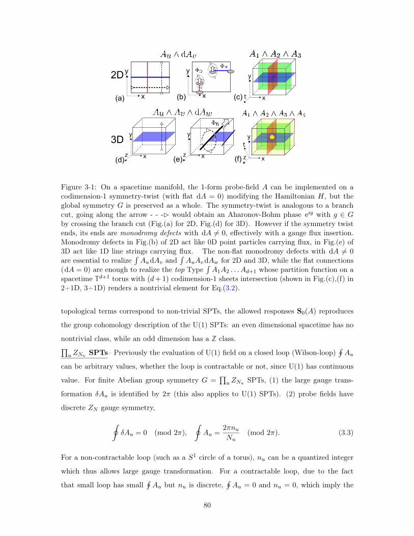
!
"
!
"
#
2D
3D
(a) (b) (c)
(d) (e)
!
"
(f)
!
"
#
!
"
#
$
!
"
#
Figure 3-1: On a spacetime manifold, the 1-form probe-field 𝐴 can be implemented on acodimension-1 symmetry-twist (with flat d𝐴 = 0) modifying the Hamiltonian 𝐻, but theglobal symmetry 𝐺 is preserved as a whole. The symmetry-twist is analogous to a branchcut, going along the arrow - - -B would obtain an Aharonov-Bohm phase e𝑖𝑔 with 𝑔 ∈ 𝐺by crossing the branch cut (Fig.(a) for 2D, Fig.(d) for 3D). However if the symmetry twistends, its ends are monodromy defects with d𝐴 = 0, effectively with a gauge flux insertion.Monodromy defects in Fig.(b) of 2D act like 0D point particles carrying flux, in Fig.(e) of3D act like 1D line strings carrying flux. The non-flat monodromy defects with d𝐴 = 0are essential to realize
∫𝐴𝑢d𝐴𝑣 and
∫𝐴𝑢𝐴𝑣d𝐴𝑤 for 2D and 3D, while the flat connections
(d𝐴 = 0) are enough to realize the top Type∫𝐴1𝐴2 . . . 𝐴𝑑+1 whose partition function on a
spacetime T𝑑+1 torus with (𝑑+1) codimension-1 sheets intersection (shown in Fig.(c),(f) in2+1D, 3+1D) renders a nontrivial element for Eq.(3.2).
topological terms correspond to non-trivial SPTs, the allowed responses S0(𝐴) reproduces
the group cohomology description of the U(1) SPTs: an even dimensional spacetime has no
nontrivial class, while an odd dimension has a Z class.∏𝑢 𝑍𝑁𝑢 SPTs– Previously the evaluation of U(1) field on a closed loop (Wilson-loop)
∮𝐴𝑢
can be arbitrary values, whether the loop is contractable or not, since U(1) has continuous
value. For finite Abelian group symmetry 𝐺 =∏𝑢 𝑍𝑁𝑢 SPTs, (1) the large gauge trans-
formation 𝛿𝐴𝑢 is identified by 2𝜋 (this also applies to U(1) SPTs). (2) probe fields have
discrete 𝑍𝑁 gauge symmetry,
∮𝛿𝐴𝑢 = 0 (mod 2𝜋),
∮𝐴𝑢 =
2𝜋𝑛𝑢𝑁𝑢
(mod 2𝜋). (3.3)
For a non-contractable loop (such as a 𝑆1 circle of a torus), 𝑛𝑢 can be a quantized integer
which thus allows large gauge transformation. For a contractable loop, due to the fact
that small loop has small∮𝐴𝑢 but 𝑛𝑢 is discrete,
∮𝐴𝑢 = 0 and 𝑛𝑢 = 0, which imply the
80

curvature d𝐴 = 0, thus 𝐴 is flat connection locally.
(i). For 1+1D, the only quantized topological term is: Z0(sym.twist) = exp[ i 𝑘II∫𝐴1𝐴2].
Here and below we omit the wedge product ∧ between gauge fields as a conventional notation.
Such a term is gauge invariant under transformation if we impose flat connection d𝐴1 =
d𝐴2 = 0, since 𝛿(𝐴1𝐴2) = (𝛿𝐴1)𝐴2+𝐴1(𝛿𝐴2) = (d𝑓1)𝐴2+𝐴1(d𝑓2) = −𝑓1(d𝐴2)−(d𝐴1)𝑓2 =
0. Here we have abandoned the surface term by considering a 1+1D closed bulk spacetime
ℳ2 without boundaries.
∙ Large gauge transformation: The invariance of Z0 under the allowed large gauge trans-
formation via Eq.(3.3) implies that the volume-integration of∫𝛿(𝐴1𝐴2) must be invariant
mod 2𝜋, namely (2𝜋)2𝑘II𝑁1
= (2𝜋)2𝑘II𝑁2
= 0 (mod 2𝜋). This rule implies the level-quantization.
∙ Flux identification: On the other hand, when the 𝑍𝑁1 flux from 𝐴1, 𝑍𝑁2 flux from 𝐴2
are inserted as 𝑛1, 𝑛2 multiple units of 2𝜋/𝑁1, 2𝜋/𝑁2, we have 𝑘II∫𝐴1𝐴2 = 𝑘II
(2𝜋)2
𝑁1𝑁2𝑛1𝑛2.
We see that 𝑘II and 𝑘′II = 𝑘II +𝑁1𝑁22𝜋 give rise to the same partition function Z0. Thus they
must be identified (2𝜋)𝑘II ≃ (2𝜋)𝑘II + 𝑁1𝑁2, as the rule of flux identification. These two
rules impose
Z0(sym.twist) = exp[ i 𝑝II𝑁1𝑁2
(2𝜋)𝑁12
∫ℳ2
𝐴1𝐴2], (3.4)
with 𝑘II = 𝑝II𝑁1𝑁2
(2𝜋)𝑁12, 𝑝II ∈ Z𝑁12 . We abbreviate the greatest common divisor (gcd)
𝑁12...𝑢 ≡ gcd(𝑁1, 𝑁2, . . . , 𝑁𝑢). Amazingly we have independently recovered the formal group
cohomology classification predicted as ℋ2(∏𝑢 𝑍𝑁𝑢 ,R/Z) =
∏𝑢<𝑣 Z𝑁𝑢𝑣 .
(ii). For 2+1D, we can propose a naive Z0(sym.twist) by dimensional counting, exp[ i 𝑘III∫𝐴1𝐴2𝐴3],
which is gauge invariant under the flat connection condition. By the large gauge transfor-
mation and the flux identification, we find that the level 𝑘III is quantized,thus
Z0(sym.twist) = exp[ i 𝑝III𝑁1𝑁2𝑁3
(2𝜋)2𝑁123
∫ℳ3
𝐴1𝐴2𝐴3], (3.5)
named as Type III SPTs with a quantized level 𝑝III ∈ Z𝑁123 . The terminology “Type”
is introduced and used in Ref.[96] and [52]. As shown in Fig.3-1, the geometric way to
understand the 1-form probe field can be regarded as (the Poincare-dual of) codimension-1
sheet assigning a group element 𝑔 ∈ 𝐺 by crossing the sheet as a branch cut. These sheets
can be regarded as the symmetry twists[?, ?] in the SPT Hamiltonian formulation. When
three sheets (𝑦𝑡, 𝑥𝑡, 𝑥𝑦 planes in Fig.3-1(c)) with nontrivial elements 𝑔𝑗 ∈ 𝑍𝑁𝑗 intersect
81
at a single point of a spacetime T3 torus, it produces a nontrivial topological invariant in
Eq.(3.2) for Type III SPTs.
There are also other types of partition functions, which require to use the insert flux
d𝐴 = 0 only at the monodromy defect (i.e. at the end of branch cut, see Fig.3-1(b)) to
probe them:
Z0(sym.twist) = exp[ i𝑝
2𝜋
∫ℳ3
𝐴𝑢d𝐴𝑣], (3.6)
where 𝑢, 𝑣 can be either the same or different gauge fields. They are Type I, II actions:
𝑝I,1∫𝐴1d𝐴1, 𝑝II,12
∫𝐴1d𝐴2, etc. In order to have e i 𝑝II
2𝜋
∫ℳ3 𝐴1 d𝐴2 invariant under the large
gauge transformation, 𝑝II must be integer. In order to have e i 𝑝I2𝜋
∫ℳ3 𝐴1 d𝐴1 well-defined,
we separate 𝐴1 = 𝐴1 + 𝐴𝐹1 to the non-flat part 𝐴1 and the flat part 𝐴𝐹1 . Its partition
function becomes e i 𝑝I2𝜋
∫ℳ3 𝐴
𝐹1 d𝐴1 . The invariance under the large gauge transformation of
𝐴𝐹1 requires 𝑝I to be quantized as integers. We can further derive their level-classification
via Eq.(3.3) and two more conditions:
∫����∫ d𝐴𝑣 = 0 (mod 2𝜋),
∫����∫ 𝛿d𝐴𝑣 = 0. (3.7)
The first means that the net sum of all monodromy-defect fluxes on the spacetime manifold
must have integer units of 2𝜋. Physically, a 2𝜋 flux configuration is trivial for a discrete
symmetry group 𝑍𝑁𝑣 . Therefore two SPT invariants differ by a 2𝜋 flux configuration on their
monodromy-defect should be regarded as the same one. The second condition means that
the variation of the total flux is zero. From the above two conditions for flux identification,
we find the SPT invariant Eq.(3.6) describes the 𝑍𝑁1 SPTs 𝑝I ∈ Z𝑁1 = ℋ3(𝑍𝑁1 ,R/Z) and
the 𝑍𝑁1 × 𝑍𝑁2 SPTs 𝑝II ∈ Z𝑁12 ⊂ ℋ3(𝑍𝑁1 × 𝑍𝑁2 ,R/Z).
(iii). For 3+1D, we derive the top Type IV partition function that is independent of
spacetime metrics:
Z0(sym.twist) = exp[i𝑝IV𝑁1𝑁2𝑁3𝑁4
(2𝜋)3𝑁1234
∫ℳ4
𝐴1𝐴2𝐴3𝐴4], (3.8)
where d𝐴𝑖 = 0 to ensure gauge invariance. The large gauge transformation 𝛿𝐴𝑖 of Eq.(3.3),
and flux identification recover 𝑝IV ∈ Z𝑁1234 ⊂ ℋ4(∏4𝑖=1 𝑍𝑁𝑖 ,R/Z). Here the 3D SPT in-
variant is analogous to 2D, when the four codimension-1 sheets (𝑦𝑧𝑡, 𝑥𝑧𝑡, 𝑦𝑧𝑡, 𝑥𝑦𝑧-branes
82
in Fig.3-1(f)) with flat 𝐴𝑗 of nontrivial element 𝑔𝑗 ∈ 𝑍𝑁𝑗 intersect at a single point on
spacetime T4 torus, it renders a nontrivial partition function for the Type IV SPTs.
Another response is for Type III 3+1D SPTs:
Z0(sym.twist) = exp[i∫ℳ4
𝑝III𝑁1𝑁2
(2𝜋)2𝑁12𝐴1𝐴2d𝐴3], (3.9)
which is gauge invariant only if d𝐴1 = d𝐴2 = 0. Based on Eq.(3.3),(3.7), the invariance
under the large gauge transformations requires 𝑝III ∈ Z𝑁123 . Eq.(3.9) describes Type III
SPTs: 𝑝III ∈ Z𝑁123 ⊂ ℋ4(∏3𝑖=1 𝑍𝑁𝑖 ,R/Z).
Yet another response is for Type II 3+1D SPTs:
Z0(sym.twist) = exp[i∫ℳ4
𝑝II𝑁1𝑁2
(2𝜋)2𝑁12𝐴1𝐴2d𝐴2]. (3.10)
The above is gauge invariant only if we choose 𝐴1 and 𝐴2 such that d𝐴1 = d𝐴2d𝐴2 = 0.
We denote 𝐴2 = 𝐴2+𝐴𝐹2 where 𝐴2d𝐴2 = 0, d𝐴𝐹2 = 0,
∮𝐴2 = 0 mod 2𝜋/𝑁2, and
∮𝐴𝐹2 = 0
mod 2𝜋/𝑁2. Note that in general d𝐴2 = 0, and Eq.(3.10) becomes ei∫ℳ4
𝑝II𝑁1𝑁2(2𝜋)2𝑁12
𝐴1𝐴𝐹2 d𝐴2 .
The invariance under the large gauge transformations of 𝐴1 and 𝐴𝐹2 and flux identification
requires 𝑝II ∈ Z𝑁12 = ℋ4(∏2𝑖=1 𝑍𝑁𝑖 ,R/Z) of Type II SPTs. For Eq.(3.9),(3.10), we have
assumed the monodromy line defect at d𝐴 = 0 is gapped ; for gapless defects, one will need
to introduce extra anomalous gapless boundary theories.
3.1.2 SPT invariants and physical probes
–
Top types: The SPT invariants can help us to design physical probes for their SPTs, as
observables of numerical simulations or real experiments. Let us consider:
Z0(sym.twist)= exp[i𝑝∏𝑑+1
𝑗=1 𝑁𝑗
(2𝜋)𝑑𝑁123...(𝑑+1)
∫𝐴1𝐴2 . . . 𝐴𝑑+1], a generic top type
∏𝑑+1𝑗=1 𝑍𝑁𝑗 SPT
invariant in (𝑑+ 1)D, and its observables.
∙ (1). Induced charges: If we design the space to have a topology (𝑆1)𝑑, and add the unit
symmetry twist of the 𝑍𝑁1 , 𝑍𝑁2 , . . . , 𝑍𝑁𝑑to the 𝑆1 in 𝑑 directions respectively:
∮𝑆1 𝐴𝑗 =
2𝜋/𝑁𝑗 . The SPT invariant implies that such a configuration will carry a 𝑍𝑁𝑑+1charge
𝑝𝑁𝑑+1
𝑁123...(𝑑+1).
∙ (2).Degenerate zero energy modes: We can also apply dimensional reduction to probe
SPTs. We can design the 𝑑D space as (𝑆1)𝑑−1 × 𝐼, and add the unit 𝑍𝑁𝑗 symmetry twists
83
along the 𝑗-th 𝑆1 circles for 𝑗 = 3, . . . , 𝑑 + 1. This induces a 1+1D 𝑍𝑁1 × 𝑍𝑁2 SPT
invariant exp[ i 𝑝 𝑁12𝑁123...(𝑑+1)
𝑁1𝑁22𝜋𝑁12
∫𝐴1𝐴2] on the 1D spatial interval 𝐼. The 0D boundary of
the reduced 1+1D SPTs has degenerate zero modes that form a projective representation
of 𝑍𝑁1 × 𝑍𝑁2 symmetry.[56] For example, dimensionally reducing 3+1D SPTs Eq.(3.8) to
this 1+1D SPTs, if we break the 𝑍𝑁3 symmetry on the 𝑍𝑁4 monodromy defect line, gapless
excitations on the defect line will be gapped. A 𝑍𝑁3 symmetry-breaking domain wall on
the gapped monodromy defect line will carry degenerate zero modes that form a projective
representation of 𝑍𝑁1 × 𝑍𝑁2 symmetry.
∙ (3).Gapless boundary excitations: For Eq.(3.8), we design the 3D space as 𝑆1 ×𝑀2, and
add the unit 𝑍𝑁4 symmetry twists along the 𝑆1 circle. Then Eq.(3.8) reduces to the 2+1D
𝑍𝑁1 × 𝑍𝑁2 × 𝑍𝑁3 SPT invariant exp[ i 𝑝IV𝑁123𝑁1234
𝑁1𝑁2𝑁32𝜋𝑁123
∫𝐴1𝐴2𝐴3] labeled by 𝑝IV
𝑁123𝑁1234
∈
Z𝑁123 ⊂ ℋ3(𝑍𝑁1×𝑍𝑁2×𝑍𝑁3 ,R/Z). Namely, the 𝑍𝑁4 monodromy line defect carries gapless
excitations identical to the edge modes of the 2+1D 𝑍𝑁1×𝑍𝑁2×𝑍𝑁3 SPTs if the symmetry
is not broken.
Lower types: Take 3+1D SPTs of Eq.(3.9) as an example, there are at least two ways to design
physical probes. First, we can design the 3D space as 𝑀2 × 𝐼, where 𝑀2 is punctured with
𝑁3 identical monodromy defects each carrying 𝑛3 unit 𝑍𝑁3 flux, namely∫����∫ d𝐴3 = 2𝜋𝑛3
of Eq.(3.7). Eq.(3.9) reduces to exp[ i 𝑝III𝑛3𝑁1𝑁2
(2𝜋)𝑁12
∫𝐴1𝐴2], which again describes a 1+1D
𝑍𝑁1 × 𝑍𝑁2 SPTs, labeled by 𝑝III𝑛3 of Eq.(3.4) in ℋ2(𝑍𝑁1 × 𝑍𝑁2 ,R/Z) = Z𝑁12 . This again
has 0D boundary-degenerate-zero-modes.
Second, we can design the 3D space as 𝑆1×𝑀2 and add a symmetry twist of 𝑍𝑁1 along
the 𝑆1:∮𝑆1 𝐴1 = 2𝜋𝑛1/𝑁1, then the SPT invariant Eq.(3.9) reduces to exp[ i 𝑝III 𝑛1𝑁2
(2𝜋)𝑁12
∫𝐴2d𝐴3],
a 2+1D 𝑍𝑁2 × 𝑍𝑁3 SPTs labeled by 𝑝III 𝑛1𝑁2
𝑁12of Eq.(3.6).
∙ (4).Defect braiding statistics and fractional charges: These∫𝐴d𝐴 types in Eq.(3.6), can
be detected by the nontrivial braiding statistics of monodromy defects, such as the parti-
cle/string defects in 2D/3D. Moreover, a 𝑍𝑁1 monodromy defect line carries gapless exci-
tations identical to the edge of the 2+1D 𝑍𝑁2 × 𝑍𝑁3 SPTs. If the gapless excitations are
gapped by 𝑍𝑁2-symmetry-breaking, its domain wall will induce fractional quantum numbers
of 𝑍𝑁3 charge,[56] similar to Jackiw-Rebbi[63] or Goldstone-Wilczek[64] effect.
U(1)𝑚 SPTs– It is straightforward to apply the above results to U(1)𝑚 symmetry. Again,
we find only trivial classes for even (𝑑+1)D. For odd (𝑑+1)D, we can define the lower type
action: Z0(sym.twist) = exp[ i 2𝜋𝑘( 𝑑+2
2)!(2𝜋)(𝑑+2)/2
∫𝐴𝑢 ∧ 𝐹𝑣 ∧ . . .]. Meanwhile we emphasize
84
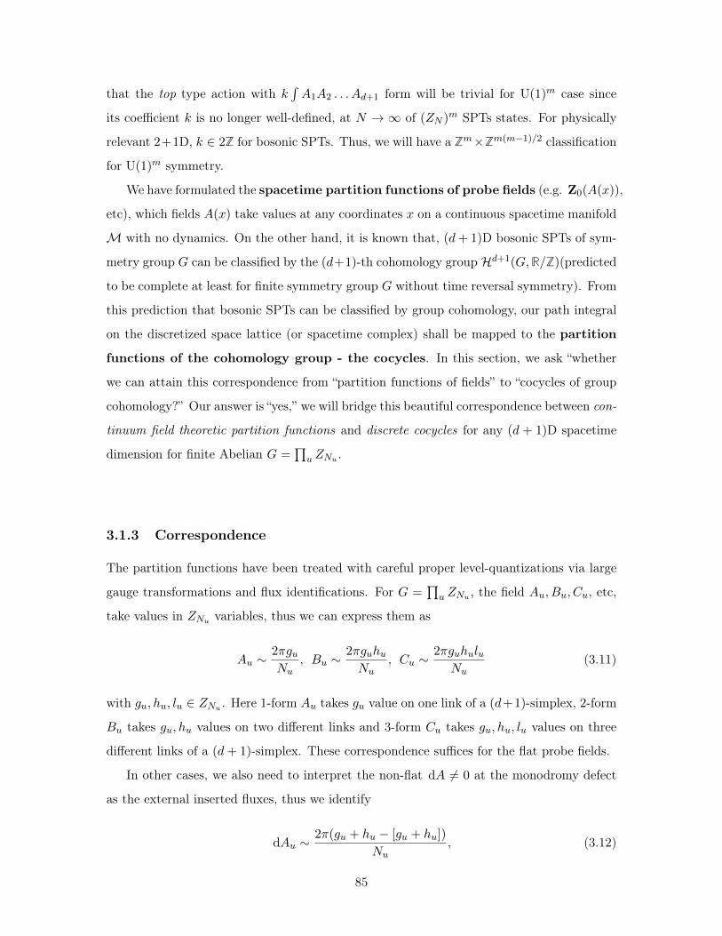
that the top type action with 𝑘∫𝐴1𝐴2 . . . 𝐴𝑑+1 form will be trivial for U(1)𝑚 case since
its coefficient 𝑘 is no longer well-defined, at 𝑁 → ∞ of (𝑍𝑁 )𝑚 SPTs states. For physically
relevant 2+1D, 𝑘 ∈ 2Z for bosonic SPTs. Thus, we will have a Z𝑚×Z𝑚(𝑚−1)/2 classification
for U(1)𝑚 symmetry.
We have formulated the spacetime partition functions of probe fields (e.g. Z0(𝐴(𝑥)),
etc), which fields 𝐴(𝑥) take values at any coordinates 𝑥 on a continuous spacetime manifold
ℳ with no dynamics. On the other hand, it is known that, (𝑑+ 1)D bosonic SPTs of sym-
metry group 𝐺 can be classified by the (𝑑+1)-th cohomology group ℋ𝑑+1(𝐺,R/Z)(predicted
to be complete at least for finite symmetry group 𝐺 without time reversal symmetry). From
this prediction that bosonic SPTs can be classified by group cohomology, our path integral
on the discretized space lattice (or spacetime complex) shall be mapped to the partition
functions of the cohomology group - the cocycles. In this section, we ask “whether
we can attain this correspondence from “partition functions of fields” to “cocycles of group
cohomology?” Our answer is “yes,” we will bridge this beautiful correspondence between con-
tinuum field theoretic partition functions and discrete cocycles for any (𝑑 + 1)D spacetime
dimension for finite Abelian 𝐺 =∏𝑢 𝑍𝑁𝑢 .
3.1.3 Correspondence
The partition functions have been treated with careful proper level-quantizations via large
gauge transformations and flux identifications. For 𝐺 =∏𝑢 𝑍𝑁𝑢 , the field 𝐴𝑢, 𝐵𝑢, 𝐶𝑢, etc,
take values in 𝑍𝑁𝑢 variables, thus we can express them as
𝐴𝑢 ∼2𝜋𝑔𝑢𝑁𝑢
, 𝐵𝑢 ∼2𝜋𝑔𝑢ℎ𝑢𝑁𝑢
, 𝐶𝑢 ∼2𝜋𝑔𝑢ℎ𝑢𝑙𝑢
𝑁𝑢(3.11)
with 𝑔𝑢, ℎ𝑢, 𝑙𝑢 ∈ 𝑍𝑁𝑢 . Here 1-form 𝐴𝑢 takes 𝑔𝑢 value on one link of a (𝑑+1)-simplex, 2-form
𝐵𝑢 takes 𝑔𝑢, ℎ𝑢 values on two different links and 3-form 𝐶𝑢 takes 𝑔𝑢, ℎ𝑢, 𝑙𝑢 values on three
different links of a (𝑑+ 1)-simplex. These correspondence suffices for the flat probe fields.
In other cases, we also need to interpret the non-flat d𝐴 = 0 at the monodromy defect
as the external inserted fluxes, thus we identify
d𝐴𝑢 ∼2𝜋(𝑔𝑢 + ℎ𝑢 − [𝑔𝑢 + ℎ𝑢])
𝑁𝑢, (3.12)
85
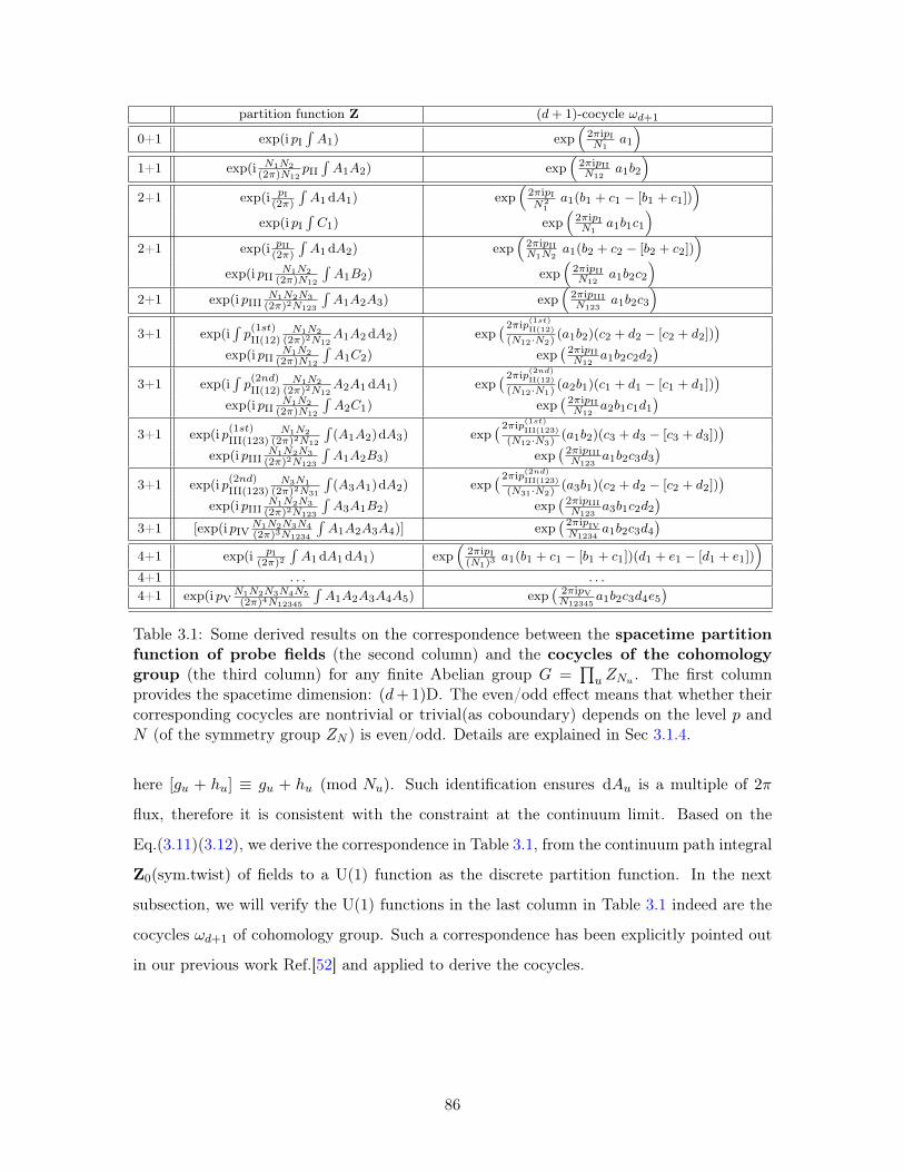
partition function Z (𝑑+ 1)-cocycle 𝜔𝑑+1
0+1 exp(i 𝑝I∫𝐴1) exp
(2𝜋i𝑝I𝑁1
𝑎1
)1+1 exp(i 𝑁1𝑁2
(2𝜋)𝑁12𝑝II
∫𝐴1𝐴2) exp
(2𝜋i𝑝II𝑁12
𝑎1𝑏2
)2+1 exp(i 𝑝I
(2𝜋)
∫𝐴1d𝐴1) exp
(2𝜋i𝑝I𝑁2
1𝑎1(𝑏1 + 𝑐1 − [𝑏1 + 𝑐1])
)exp(i 𝑝I
∫𝐶1) exp
(2𝜋i𝑝I𝑁1
𝑎1𝑏1𝑐1
)2+1 exp(i 𝑝II
(2𝜋)
∫𝐴1d𝐴2) exp
(2𝜋i𝑝II𝑁1𝑁2
𝑎1(𝑏2 + 𝑐2 − [𝑏2 + 𝑐2]))
exp(i 𝑝II𝑁1𝑁2
(2𝜋)𝑁12
∫𝐴1𝐵2) exp
(2𝜋i𝑝II𝑁12
𝑎1𝑏2𝑐2
)2+1 exp(i 𝑝III
𝑁1𝑁2𝑁3
(2𝜋)2𝑁123
∫𝐴1𝐴2𝐴3) exp
(2𝜋i𝑝III𝑁123
𝑎1𝑏2𝑐3
)3+1 exp(i
∫𝑝(1𝑠𝑡)II(12)
𝑁1𝑁2
(2𝜋)2𝑁12𝐴1𝐴2d𝐴2) exp
( 2𝜋i𝑝(1𝑠𝑡)
II(12)(𝑁12·𝑁2)
(𝑎1𝑏2)(𝑐2 + 𝑑2 − [𝑐2 + 𝑑2]))
exp(i 𝑝II𝑁1𝑁2
(2𝜋)𝑁12
∫𝐴1𝐶2) exp
( 2𝜋i𝑝II𝑁12
𝑎1𝑏2𝑐2𝑑2)
3+1 exp(i∫𝑝(2𝑛𝑑)II(12)
𝑁1𝑁2
(2𝜋)2𝑁12𝐴2𝐴1d𝐴1) exp
( 2𝜋i𝑝(2𝑛𝑑)
II(12)(𝑁12·𝑁1)
(𝑎2𝑏1)(𝑐1 + 𝑑1 − [𝑐1 + 𝑑1]))
exp(i 𝑝II𝑁1𝑁2
(2𝜋)𝑁12
∫𝐴2𝐶1) exp
( 2𝜋i𝑝II𝑁12
𝑎2𝑏1𝑐1𝑑1)
3+1 exp(i 𝑝(1𝑠𝑡)III(123)𝑁1𝑁2
(2𝜋)2𝑁12
∫(𝐴1𝐴2)d𝐴3) exp
( 2𝜋i𝑝(1𝑠𝑡)
III(123)(𝑁12·𝑁3)
(𝑎1𝑏2)(𝑐3 + 𝑑3 − [𝑐3 + 𝑑3]))
exp(i 𝑝III𝑁1𝑁2𝑁3
(2𝜋)2𝑁123
∫𝐴1𝐴2𝐵3) exp
( 2𝜋i𝑝III𝑁123
𝑎1𝑏2𝑐3𝑑3)
3+1 exp(i 𝑝(2𝑛𝑑)III(123)𝑁3𝑁1
(2𝜋)2𝑁31
∫(𝐴3𝐴1)d𝐴2) exp
( 2𝜋i𝑝(2𝑛𝑑)
III(123)(𝑁31·𝑁2)
(𝑎3𝑏1)(𝑐2 + 𝑑2 − [𝑐2 + 𝑑2]))
exp(i 𝑝III𝑁1𝑁2𝑁3
(2𝜋)2𝑁123
∫𝐴3𝐴1𝐵2) exp
( 2𝜋i𝑝III𝑁123
𝑎3𝑏1𝑐2𝑑2)
3+1 [exp(i 𝑝IV𝑁1𝑁2𝑁3𝑁4
(2𝜋)3𝑁1234
∫𝐴1𝐴2𝐴3𝐴4)] exp
( 2𝜋i𝑝IV𝑁1234
𝑎1𝑏2𝑐3𝑑4)
4+1 exp(i 𝑝I(2𝜋)2
∫𝐴1d𝐴1d𝐴1) exp
(2𝜋i𝑝I(𝑁1)3
𝑎1(𝑏1 + 𝑐1 − [𝑏1 + 𝑐1])(𝑑1 + 𝑒1 − [𝑑1 + 𝑒1]))
4+1 . . . . . .
4+1 exp(i 𝑝V𝑁1𝑁2𝑁3𝑁4𝑁5
(2𝜋)4𝑁12345
∫𝐴1𝐴2𝐴3𝐴4𝐴5) exp
( 2𝜋i𝑝V𝑁12345
𝑎1𝑏2𝑐3𝑑4𝑒5)
Table 3.1: Some derived results on the correspondence between the spacetime partitionfunction of probe fields (the second column) and the cocycles of the cohomologygroup (the third column) for any finite Abelian group 𝐺 =
∏𝑢 𝑍𝑁𝑢 . The first column
provides the spacetime dimension: (𝑑+1)D. The even/odd effect means that whether theircorresponding cocycles are nontrivial or trivial(as coboundary) depends on the level 𝑝 and𝑁 (of the symmetry group 𝑍𝑁 ) is even/odd. Details are explained in Sec 3.1.4.
here [𝑔𝑢 + ℎ𝑢] ≡ 𝑔𝑢 + ℎ𝑢 (mod 𝑁𝑢). Such identification ensures d𝐴𝑢 is a multiple of 2𝜋
flux, therefore it is consistent with the constraint at the continuum limit. Based on the
Eq.(3.11)(3.12), we derive the correspondence in Table 3.1, from the continuum path integral
Z0(sym.twist) of fields to a U(1) function as the discrete partition function. In the next
subsection, we will verify the U(1) functions in the last column in Table 3.1 indeed are the
cocycles 𝜔𝑑+1 of cohomology group. Such a correspondence has been explicitly pointed out
in our previous work Ref.[52] and applied to derive the cocycles.
86
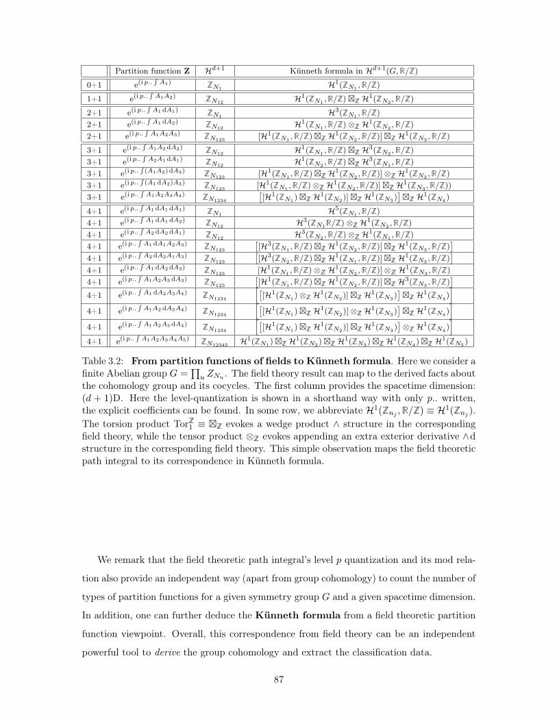
Partition function Z ℋ𝑑+1 Künneth formula in ℋ𝑑+1(𝐺,R/Z)
0+1 e(i 𝑝..∫𝐴1) Z𝑁1
ℋ1(Z𝑁1,R/Z)
1+1 e(i 𝑝..∫𝐴1𝐴2) Z𝑁12
ℋ1(Z𝑁1,R/Z)�Z ℋ1(Z𝑁2
,R/Z)
2+1 e(i 𝑝..∫𝐴1 d𝐴1) Z𝑁1
ℋ3(Z𝑁1,R/Z)
2+1 e(i 𝑝..∫𝐴1 d𝐴2) Z𝑁12
ℋ1(Z𝑁1,R/Z)⊗Z ℋ1(Z𝑁2
,R/Z)
2+1 e(i 𝑝..∫𝐴1𝐴2𝐴3) Z𝑁123
[ℋ1(Z𝑁1,R/Z)�Z ℋ1(Z𝑁2
,R/Z)]�Z ℋ1(Z𝑁3,R/Z)
3+1 e(i 𝑝..∫𝐴1𝐴2 d𝐴2) Z𝑁12
ℋ1(Z𝑁1,R/Z)�Z ℋ3(Z𝑁2
,R/Z)
3+1 e(i 𝑝..∫𝐴2𝐴1 d𝐴1) Z𝑁12
ℋ1(Z𝑁2,R/Z)�Z ℋ3(Z𝑁1
,R/Z)
3+1 e(i 𝑝..∫(𝐴1𝐴2)d𝐴3) Z𝑁123
[ℋ1(Z𝑁1,R/Z)�Z ℋ1(Z𝑁2
,R/Z)]⊗Z ℋ1(Z𝑁3,R/Z)
3+1 e(i 𝑝..∫(𝐴1 d𝐴2)𝐴3) Z𝑁123
[ℋ1(Z𝑁1,R/Z)⊗Z ℋ1(Z𝑁2
,R/Z)]�Z ℋ1(Z𝑁3,R/Z))
3+1 e(i 𝑝..∫𝐴1𝐴2𝐴3𝐴4) Z𝑁1234
[[ℋ1(Z𝑁1
)�Z ℋ1(Z𝑁2)]�Z ℋ1(Z𝑁3
)]�Z ℋ1(Z𝑁4
)
4+1 e(i 𝑝..∫𝐴1 d𝐴1 d𝐴1) Z𝑁1
ℋ5(Z𝑁1,R/Z)
4+1 e(i 𝑝..∫𝐴1 d𝐴1 d𝐴2) Z𝑁12
ℋ3(Z𝑁1R/Z)⊗Z ℋ1(Z𝑁2
,R/Z)
4+1 e(i 𝑝..∫𝐴2 d𝐴2 d𝐴1) Z𝑁12
ℋ3(Z𝑁2,R/Z)⊗Z ℋ1(Z𝑁1
,R/Z)
4+1 e(i 𝑝..∫𝐴1 d𝐴1𝐴2𝐴3) Z𝑁123
[[ℋ3(Z𝑁1
,R/Z)�Z ℋ1(Z𝑁2,R/Z)]�Z ℋ1(Z𝑁3
,R/Z)]
4+1 e(i 𝑝..∫𝐴2 d𝐴2𝐴1𝐴3) Z𝑁123
[[ℋ3(Z𝑁2
,R/Z)�Z ℋ1(Z𝑁1,R/Z)]�Z ℋ1(Z𝑁3
,R/Z)]
4+1 e(i 𝑝..∫𝐴1 d𝐴2 d𝐴3) Z𝑁123
[ℋ1(Z𝑁1,R/Z)⊗𝑍 ℋ1(Z𝑁2
,R/Z)]⊗𝑍 ℋ1(Z𝑁3,R/Z)
4+1 e(i 𝑝..∫𝐴1𝐴2𝐴3 d𝐴3) Z𝑁123
[[ℋ1(Z𝑁1
,R/Z)�Z ℋ1(Z𝑁2,R/Z)]�Z ℋ3(Z𝑁3
,R/Z)]
4+1 e(i 𝑝..∫𝐴1 d𝐴2𝐴3𝐴4) Z𝑁1234
[[[ℋ1(Z𝑁1
)⊗Z ℋ1(Z𝑁2)]�Z ℋ1(Z𝑁3
)]�Z ℋ1(Z𝑁4
)]
4+1 e(i 𝑝..∫𝐴1𝐴2 d𝐴3𝐴4) Z𝑁1234
[[[ℋ1(Z𝑁1
)�Z ℋ1(Z𝑁2)]⊗Z ℋ1(Z𝑁3
)]�Z ℋ1(Z𝑁4
)]
4+1 e(i 𝑝..∫𝐴1𝐴2𝐴3 d𝐴4) Z𝑁1234
[[[ℋ1(Z𝑁1
)�Z ℋ1(Z𝑁2)]�Z ℋ1(Z𝑁3
)]⊗Z ℋ1(Z𝑁4
)]
4+1 e(i 𝑝..∫𝐴1𝐴2𝐴3𝐴4𝐴5) Z𝑁12345
ℋ1(Z𝑁1)�Z ℋ1(Z𝑁2
)�Z ℋ1(Z𝑁3)�Z ℋ1(Z𝑁4
)�Z ℋ1(Z𝑁5)
Table 3.2: From partition functions of fields to Künneth formula. Here we consider afinite Abelian group 𝐺 =
∏𝑢 𝑍𝑁𝑢 . The field theory result can map to the derived facts about
the cohomology group and its cocycles. The first column provides the spacetime dimension:(𝑑 + 1)D. Here the level-quantization is shown in a shorthand way with only 𝑝.. written,the explicit coefficients can be found. In some row, we abbreviate ℋ1(Z𝑛𝑗 ,R/Z) ≡ ℋ1(Z𝑛𝑗 ).The torsion product TorZ
1 ≡ �Z evokes a wedge product ∧ structure in the correspondingfield theory, while the tensor product ⊗Z evokes appending an extra exterior derivative ∧dstructure in the corresponding field theory. This simple observation maps the field theoreticpath integral to its correspondence in Künneth formula.
We remark that the field theoretic path integral’s level 𝑝 quantization and its mod rela-
tion also provide an independent way (apart from group cohomology) to count the number of
types of partition functions for a given symmetry group 𝐺 and a given spacetime dimension.
In addition, one can further deduce the Künneth formula from a field theoretic partition
function viewpoint. Overall, this correspondence from field theory can be an independent
powerful tool to derive the group cohomology and extract the classification data.
87
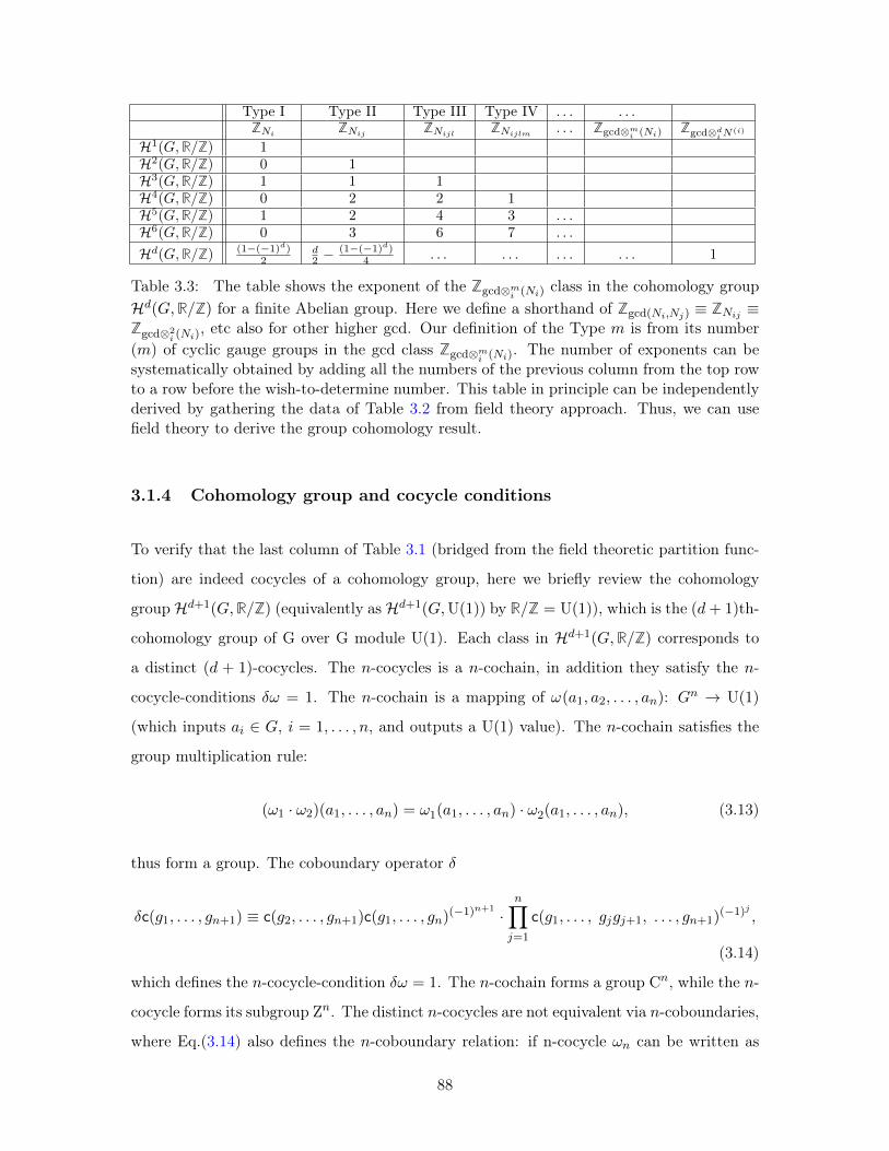
Type I Type II Type III Type IV . . . . . .Z𝑁𝑖
Z𝑁𝑖𝑗Z𝑁𝑖𝑗𝑙
Z𝑁𝑖𝑗𝑙𝑚. . . Zgcd⊗𝑚
𝑖 (𝑁𝑖) Zgcd⊗𝑑𝑖 𝑁
(𝑖)
ℋ1(𝐺,R/Z) 1ℋ2(𝐺,R/Z) 0 1ℋ3(𝐺,R/Z) 1 1 1ℋ4(𝐺,R/Z) 0 2 2 1ℋ5(𝐺,R/Z) 1 2 4 3 . . .ℋ6(𝐺,R/Z) 0 3 6 7 . . .
ℋ𝑑(𝐺,R/Z) (1−(−1)𝑑)2
𝑑2 −
(1−(−1)𝑑)4 . . . . . . . . . . . . 1
Table 3.3: The table shows the exponent of the Zgcd⊗𝑚𝑖 (𝑁𝑖) class in the cohomology group
ℋ𝑑(𝐺,R/Z) for a finite Abelian group. Here we define a shorthand of Zgcd(𝑁𝑖,𝑁𝑗) ≡ Z𝑁𝑖𝑗 ≡Zgcd⊗2
𝑖 (𝑁𝑖), etc also for other higher gcd. Our definition of the Type 𝑚 is from its number
(𝑚) of cyclic gauge groups in the gcd class Zgcd⊗𝑚𝑖 (𝑁𝑖). The number of exponents can be
systematically obtained by adding all the numbers of the previous column from the top rowto a row before the wish-to-determine number. This table in principle can be independentlyderived by gathering the data of Table 3.2 from field theory approach. Thus, we can usefield theory to derive the group cohomology result.
3.1.4 Cohomology group and cocycle conditions
To verify that the last column of Table 3.1 (bridged from the field theoretic partition func-
tion) are indeed cocycles of a cohomology group, here we briefly review the cohomology
groupℋ𝑑+1(𝐺,R/Z) (equivalently asℋ𝑑+1(𝐺,U(1)) by R/Z = U(1)), which is the (𝑑+ 1)th-
cohomology group of G over G module U(1). Each class in ℋ𝑑+1(𝐺,R/Z) corresponds to
a distinct (𝑑 + 1)-cocycles. The 𝑛-cocycles is a 𝑛-cochain, in addition they satisfy the 𝑛-
cocycle-conditions 𝛿𝜔 = 1. The 𝑛-cochain is a mapping of 𝜔(𝑎1, 𝑎2, . . . , 𝑎𝑛): 𝐺𝑛 → U(1)
(which inputs 𝑎𝑖 ∈ 𝐺, 𝑖 = 1, . . . , 𝑛, and outputs a U(1) value). The 𝑛-cochain satisfies the
group multiplication rule:
(𝜔1 · 𝜔2)(𝑎1, . . . , 𝑎𝑛) = 𝜔1(𝑎1, . . . , 𝑎𝑛) · 𝜔2(𝑎1, . . . , 𝑎𝑛), (3.13)
thus form a group. The coboundary operator 𝛿
𝛿c(𝑔1, . . . , 𝑔𝑛+1) ≡ c(𝑔2, . . . , 𝑔𝑛+1)c(𝑔1, . . . , 𝑔𝑛)(−1)𝑛+1 ·
𝑛∏𝑗=1
c(𝑔1, . . . , 𝑔𝑗𝑔𝑗+1, . . . , 𝑔𝑛+1)(−1)𝑗 ,
(3.14)
which defines the 𝑛-cocycle-condition 𝛿𝜔 = 1. The 𝑛-cochain forms a group C𝑛, while the 𝑛-
cocycle forms its subgroup Z𝑛. The distinct 𝑛-cocycles are not equivalent via 𝑛-coboundaries,
where Eq.(3.14) also defines the 𝑛-coboundary relation: if n-cocycle 𝜔𝑛 can be written as
88
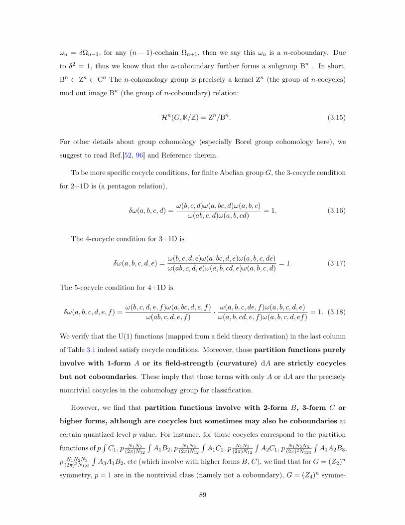
𝜔𝑛 = 𝛿Ω𝑛−1, for any (𝑛 − 1)-cochain Ω𝑛+1, then we say this 𝜔𝑛 is a 𝑛-coboundary. Due
to 𝛿2 = 1, thus we know that the 𝑛-coboundary further forms a subgroup B𝑛 . In short,
B𝑛 ⊂ Z𝑛 ⊂ C𝑛 The 𝑛-cohomology group is precisely a kernel Z𝑛 (the group of 𝑛-cocycles)
mod out image B𝑛 (the group of 𝑛-coboundary) relation:
ℋ𝑛(𝐺,R/Z) = Z𝑛/B𝑛. (3.15)
For other details about group cohomology (especially Borel group cohomology here), we
suggest to read Ref.[52, 96] and Reference therein.
To be more specific cocycle conditions, for finite Abelian group 𝐺, the 3-cocycle condition
for 2+1D is (a pentagon relation),
𝛿𝜔(𝑎, 𝑏, 𝑐, 𝑑) =𝜔(𝑏, 𝑐, 𝑑)𝜔(𝑎, 𝑏𝑐, 𝑑)𝜔(𝑎, 𝑏, 𝑐)
𝜔(𝑎𝑏, 𝑐, 𝑑)𝜔(𝑎, 𝑏, 𝑐𝑑)= 1. (3.16)
The 4-cocycle condition for 3+1D is
𝛿𝜔(𝑎, 𝑏, 𝑐, 𝑑, 𝑒) =𝜔(𝑏, 𝑐, 𝑑, 𝑒)𝜔(𝑎, 𝑏𝑐, 𝑑, 𝑒)𝜔(𝑎, 𝑏, 𝑐, 𝑑𝑒)
𝜔(𝑎𝑏, 𝑐, 𝑑, 𝑒)𝜔(𝑎, 𝑏, 𝑐𝑑, 𝑒)𝜔(𝑎, 𝑏, 𝑐, 𝑑)= 1. (3.17)
The 5-cocycle condition for 4+1D is
𝛿𝜔(𝑎, 𝑏, 𝑐, 𝑑, 𝑒, 𝑓) =𝜔(𝑏, 𝑐, 𝑑, 𝑒, 𝑓)𝜔(𝑎, 𝑏𝑐, 𝑑, 𝑒, 𝑓)
𝜔(𝑎𝑏, 𝑐, 𝑑, 𝑒, 𝑓)· 𝜔(𝑎, 𝑏, 𝑐, 𝑑𝑒, 𝑓)𝜔(𝑎, 𝑏, 𝑐, 𝑑, 𝑒)𝜔(𝑎, 𝑏, 𝑐𝑑, 𝑒, 𝑓)𝜔(𝑎, 𝑏, 𝑐, 𝑑, 𝑒𝑓)
= 1. (3.18)
We verify that the U(1) functions (mapped from a field theory derivation) in the last column
of Table 3.1 indeed satisfy cocycle conditions. Moreover, those partition functions purely
involve with 1-form 𝐴 or its field-strength (curvature) d𝐴 are strictly cocycles
but not coboundaries. These imply that those terms with only 𝐴 or d𝐴 are the precisely
nontrivial cocycles in the cohomology group for classification.
However, we find that partition functions involve with 2-form 𝐵, 3-form 𝐶 or
higher forms, although are cocycles but sometimes may also be coboundaries at
certain quantized level 𝑝 value. For instance, for those cocycles correspond to the partition
functions of 𝑝∫𝐶1, 𝑝 𝑁1𝑁2
(2𝜋)𝑁12
∫𝐴1𝐵2, 𝑝 𝑁1𝑁2
(2𝜋)𝑁12
∫𝐴1𝐶2, 𝑝 𝑁1𝑁2
(2𝜋)𝑁12
∫𝐴2𝐶1, 𝑝 𝑁1𝑁2𝑁3
(2𝜋)2𝑁123
∫𝐴1𝐴2𝐵3,
𝑝 𝑁1𝑁2𝑁3(2𝜋)2𝑁123
∫𝐴3𝐴1𝐵2, etc (which involve with higher forms 𝐵, 𝐶), we find that for 𝐺 = (𝑍2)
𝑛
symmetry, 𝑝 = 1 are in the nontrivial class (namely not a coboundary), 𝐺 = (𝑍4)𝑛 symme-
89
try, 𝑝 = 1, 3 are in the nontrivial class (namely not a coboundary). However, for 𝐺 = (𝑍3)𝑛
symmetry of all 𝑝 and 𝐺 = (𝑍4)𝑛 symmetry at 𝑝 = 2, are in the trivial class (namely a
coboundary), etc. This indicates an even-odd effect, sometimes these cocycles are non-
trivial, but sometimes are trivial as coboundary, depending on the level 𝑝 is even/odd and
the symmetry group (𝑍𝑁 )𝑛 whether 𝑁 is even/odd. Such an even/odd effect also bring
complication into the validity of nontrivial cocycles, thus this is another reason
that we study only field theory involves with only 1-form 𝐴 or its field strength
d𝐴. The cocycles composed from 𝐴 and d𝐴 in Table 3.1 are always nontrivial
and are not coboundaries.
We finally point out that the concept of boundary term in field theory (the surface
or total derivative term) is connected to the concept of coboundary in the cohomol-
ogy group. For example,∫(d𝐴1)𝐴2𝐴3 are identified as the coboundary of the linear
combination of∫𝐴1𝐴2(d𝐴3) and
∫𝐴1(d𝐴2)𝐴3. Thus, by counting the number of distinct
field theoretic actions (not identified by boundary term) is precisely counting the num-
ber of distinct field theoretic actions (not identified by coboundary). Such an observation
matches the field theory classification to the group cohomology classification. Furthermore,
we can map the field theory result to the Künneth formula listed via the correspondence:
∫𝐴1 ∼ ℋ1(Z𝑁1 ,R/Z) (3.19)∫
𝐴1d𝐴1 ∼ ℋ3(Z𝑁1 ,R/Z) (3.20)∫𝐴1d𝐴1d𝐴1 ∼ ℋ5(Z𝑁1 ,R/Z) (3.21)
TorZ1 ≡ �Z ∼ ∧ (3.22)
⊗Z ∼ ∧d (3.23)∫𝐴1 ∧𝐴2 ∼ ℋ1(Z𝑁1 ,R/Z)�Z ℋ1(Z𝑁2 ,R/Z) (3.24)∫𝐴1 ∧ d𝐴2 ∼ ℋ1(Z𝑁1 ,R/Z)⊗Z ℋ1(Z𝑁2 ,R/Z) (3.25)
. . .
To summarize, in this section, we show that, at lease for finite Abelian symmetry group
𝐺 =∏𝑘𝑖=1 𝑍𝑁𝑖 , field theory can be systematically formulated, via the level-quantization
developed earlier, we can count the number of classes of SPTs. Explicit examples are or-
90
ganized in Table 3.1 where we show that our field theory approach can exhaust all bosonic
SPT classes (at least as complete as) in group cohomology:
ℋ2(𝐺,R/Z) =∏
1≤𝑖<𝑗≤𝑘Z𝑁𝑖𝑗 (3.26)
ℋ3(𝐺,R/Z) =∏
1≤𝑖<𝑗<𝑙≤𝑘Z𝑁𝑖 × Z𝑁𝑖𝑗 × Z𝑁𝑖𝑗𝑙
(3.27)
ℋ4(𝐺,R/Z) =∏
1≤𝑖<𝑗<𝑙<𝑚≤𝑘(Z𝑁𝑖𝑗 )
2 × (Z𝑁𝑖𝑗𝑙)2 × Z𝑁𝑖𝑗𝑙𝑚
(3.28)
. . .
and we also had addressed the correspondence between field theory and Künneth formula.
3.1.5 Summary
– The recently-found SPTs, described by group cohomology, have SPT invariants in terms
of pure gauge actions (whose boundaries have pure gauge anomalies[49, 50, 56, 88, 89]).
We have derived the formal group cohomology results from an easily-accessible field theory
set-up. For beyond-group-cohomology SPT invariants, while ours of bulk-onsite-unitary
symmetry are mixed gauge-gravity actions, those of other symmetries (e.g. anti-unitary-
symmetry time-reversal Z𝑇2 ) may be pure gravity actions.[92] SPT invariants can also be
obtained via cobordism theory,[91, 92, 90] or via gauge-gravity actions whose boundaries
realizing gauge-gravitational anomalies. We have incorporated this idea into a field theoretic
framework, which should be applicable for both bosonic and fermionic SPTs and for more
exotic states awaiting future explorations.
3.2 Induced Fractional Quantum Numbers and Degenerate
Zero Modes: the anomalous edge physics of Symmetry-
Protected Topological States
We will now focus on 2+1D bulk/1+1D edge and go further to consider the edge modes of
lattice Hamiltonian with 𝐺 = 𝑍𝑁1 × 𝑍𝑁2 × 𝑍𝑁3 symmetry on a compact ring with 𝑀 sites
91
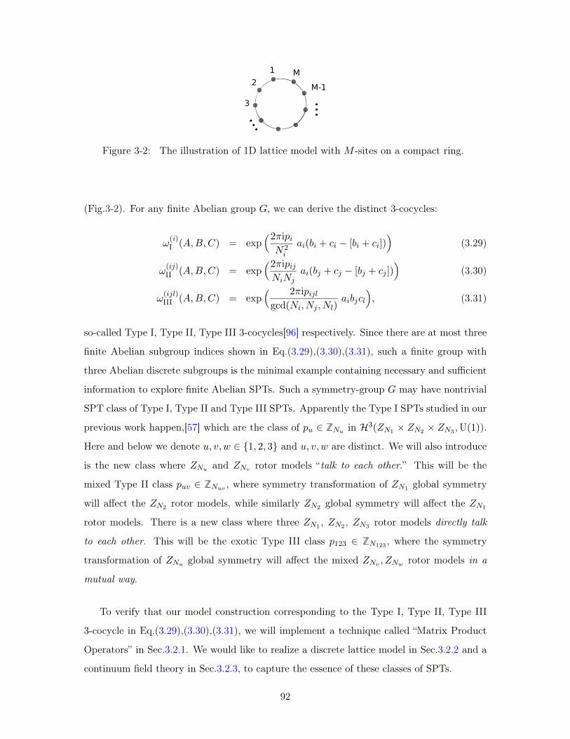
1
2M
M-1
3
......
Figure 3-2: The illustration of 1D lattice model with 𝑀 -sites on a compact ring.
(Fig.3-2). For any finite Abelian group 𝐺, we can derive the distinct 3-cocycles:
𝜔(𝑖)I (𝐴,𝐵,𝐶) = exp
(2𝜋i𝑝𝑖𝑁2𝑖
𝑎𝑖(𝑏𝑖 + 𝑐𝑖 − [𝑏𝑖 + 𝑐𝑖]))
(3.29)
𝜔(𝑖𝑗)II (𝐴,𝐵,𝐶) = exp
(2𝜋i𝑝𝑖𝑗𝑁𝑖𝑁𝑗
𝑎𝑖(𝑏𝑗 + 𝑐𝑗 − [𝑏𝑗 + 𝑐𝑗 ]))
(3.30)
𝜔(𝑖𝑗𝑙)III (𝐴,𝐵,𝐶) = exp
( 2𝜋i𝑝𝑖𝑗𝑙gcd(𝑁𝑖, 𝑁𝑗 , 𝑁𝑙)
𝑎𝑖𝑏𝑗𝑐𝑙
), (3.31)
so-called Type I, Type II, Type III 3-cocycles[96] respectively. Since there are at most three
finite Abelian subgroup indices shown in Eq.(3.29),(3.30),(3.31), such a finite group with
three Abelian discrete subgroups is the minimal example containing necessary and sufficient
information to explore finite Abelian SPTs. Such a symmetry-group 𝐺 may have nontrivial
SPT class of Type I, Type II and Type III SPTs. Apparently the Type I SPTs studied in our
previous work happen,[57] which are the class of 𝑝𝑢 ∈ Z𝑁𝑢 in ℋ3(𝑍𝑁1 × 𝑍𝑁2 × 𝑍𝑁3 ,U(1)).
Here and below we denote 𝑢, 𝑣, 𝑤 ∈ {1, 2, 3} and 𝑢, 𝑣, 𝑤 are distinct. We will also introduce
is the new class where 𝑍𝑁𝑢 and 𝑍𝑁𝑣 rotor models “talk to each other.” This will be the
mixed Type II class 𝑝𝑢𝑣 ∈ Z𝑁𝑢𝑣 , where symmetry transformation of 𝑍𝑁1 global symmetry
will affect the 𝑍𝑁2 rotor models, while similarly 𝑍𝑁2 global symmetry will affect the 𝑍𝑁1
rotor models. There is a new class where three 𝑍𝑁1 , 𝑍𝑁2 , 𝑍𝑁3 rotor models directly talk
to each other. This will be the exotic Type III class 𝑝123 ∈ Z𝑁123 , where the symmetry
transformation of 𝑍𝑁𝑢 global symmetry will affect the mixed 𝑍𝑁𝑣 , 𝑍𝑁𝑤 rotor models in a
mutual way.
To verify that our model construction corresponding to the Type I, Type II, Type III
3-cocycle in Eq.(3.29),(3.30),(3.31), we will implement a technique called “Matrix Product
Operators” in Sec.3.2.1. We would like to realize a discrete lattice model in Sec.3.2.2 and a
continuum field theory in Sec.3.2.3, to capture the essence of these classes of SPTs.
92
3.2.1 Matrix Product Operators and Cocycles
There are various advantages to put a quantum system on a discretize lattice, better than
viewing it as a continuum field theory. For example, one advantage is that the sym-
metry transformation can be regularized so to understand its property such as onsite or
non-onsite. Another advantage is that we can simulate our model by considering a dis-
cretized finite system with a finite dimensional Hilbert space. For our purpose, to regu-
larize a quantum system on a discrete lattice, we will firstly use the matrix product op-
erators (MPO) formalism (see Ref.[97] and Reference therein) to formulate our symmetry
transformations corresponding to non-trivial 3-cocycles in the third cohomology group in
ℋ3(𝑍𝑁1 × 𝑍𝑁2 ,U(1)) = Z𝑁1 × Z𝑁2 × Z𝑁12 .
First we formulate the unitary operator 𝑆 as the MPO:
𝑆 =∑{𝑗,𝑗′}
tr[𝑇𝑗1𝑗′1𝛼1𝛼2𝑇
𝑗2𝑗′2𝛼2𝛼3 . . . 𝑇
𝑗𝑀 𝑗′𝑀𝛼𝑀𝛼1 ]|𝑗′1, . . . , 𝑗′𝑀 ⟩⟨𝑗1, . . . , 𝑗𝑀 |. (3.32)
with the its coefficient taking the trace (tr) of a series of onsite tensor 𝑇 (𝑔) on a lattice,
and input a state |𝑗1, . . . , 𝑗𝑀 ⟩ and output another state |𝑗′1, . . . , 𝑗′𝑀 ⟩. 𝑇 = 𝑇 (𝑔) is a ten-
sor with multi-indices and with dependency on a group element 𝑔 ∈ 𝐺 for a symmetry
group. This is the operator formalism of matrix product states (MPS). Here physical indices
𝑗1, 𝑗2, . . . , 𝑗𝑀 and 𝑗′1, 𝑗′2, . . . , 𝑗
′𝑀 are labeled by input/output physical eigenvalues (here 𝑍𝑁
rotor angle), the subindices 1, 2, . . . ,𝑀 are the physical site indices. There are also virtual
indices 𝛼1, 𝛼2, . . . , 𝛼𝑀 which are traced in the end. Summing over all the operation from
{𝑗, 𝑗′} indices, we shall reproduce the symmetry transformation operator 𝑆. What MPO
really helps us is that
by contracting MPO tensors 𝑇 (𝑔) of 𝐺-symmetry transformation 𝑆 (here 𝑔 ∈ 𝐺) in differ-
ent sequence on the effective 1D lattice of SPT edge modes, it can reveal the nontrivial
projective phase corresponds to the nontrivial 3-cocycles of the cohomology group.
To find out the projective phase 𝑒𝑖𝜃(𝑔𝑎,𝑔𝑏,𝑔𝑐), below we use the facts of tensors 𝑇 (𝑔𝑎),
𝑇 (𝑔𝑏), 𝑇 (𝑔𝑐) acting on the same site with group elements 𝑔𝑎, 𝑔𝑏, 𝑔𝑐. We know a generic
projective relation:
𝑇 (𝑔𝑎 · 𝑔𝑏) = 𝑃 †𝑔𝑎,𝑔𝑏
𝑇 (𝑔𝑎)𝑇 (𝑔𝑏)𝑃𝑔𝑎,𝑔𝑏 . (3.33)
93
Here 𝑃𝑔𝑎,𝑔𝑏 is the projection operator. We contract three tensors in two different orders,
(𝑃𝑔𝑎,𝑔𝑏⊗𝐼3)𝑃𝑔𝑎𝑔𝑏,𝑔𝑐 ≃ 𝑒i𝜃(𝑔𝑎,𝑔𝑏,𝑔𝑐)(𝐼1 ⊗ 𝑃𝑔𝑏,𝑔𝑐)𝑃𝑔𝑎,𝑔𝑏𝑔𝑐 . (3.34)
The left-hand-side contracts the 𝑎, 𝑏 first then with the 𝑐, while the right-hand-side contracts
the 𝑏, 𝑐 first then with the 𝑎. Here ≃ means the equivalence is up to a projection out of
un-parallel states. We can derive 𝑃𝑔𝑎,𝑔𝑏 by observing that 𝑃𝑔𝑎,𝑔𝑏 inputs one state and outputs
two states.
For Type I SPT class, this MPO formalism has been done quite carefully in Ref.[97],[57].
Here we generalize it to other SPTs, below we input a group element with 𝑔 = (𝑘1, 𝑘2, 𝑘3)
and 𝑘1 ∈ 𝑍𝑁1 , 𝑘2 ∈ 𝑍𝑁2 , 𝑘3 ∈ 𝑍𝑁3 . Without losing generality, we focus on the symmetry
Type I index 𝑝1 ∈ Z𝑁1 , Type II index 𝑝12 ∈ Z𝑁12 , Type III index 𝑝123 ∈ Z𝑁123 . By index
relabeling, we can fulfill all SPT symmetries within the classification.
We propose our 𝑇 (𝑔) tensor for Type I, [97, 57] II symmetry with 𝑝1 ∈ Z𝑁1 , 𝑝12 ∈ Z𝑁12
as
(𝑇 𝜑(1)𝑖𝑛 ,𝜑
(1)𝑜𝑢𝑡,𝜑
(2)𝑖𝑛 ,𝜑
(2)𝑜𝑢𝑡)
(𝑝1,𝑝12)
𝜙(1)𝛼 ,𝜙
(1)𝛽 ,𝜙
(2)𝛼 ,𝜙
(2)𝛽 ,𝑁1
(2𝜋𝑘1𝑁1
) = 𝛿(𝜑(1)𝑜𝑢𝑡 − 𝜑
(1)𝑖𝑛 −
2𝜋𝑘1𝑁1
)𝛿(𝜑(2)𝑜𝑢𝑡 − 𝜑
(2)𝑖𝑛 )
·∫
d𝜙(1)𝛼 𝑑𝜙
(1)𝛽 |𝜙
(1)𝛽 ⟩⟨𝜙
(1)𝛼 |𝛿(𝜙
(1)𝛽 − 𝜑
(1)𝑖𝑛 )𝑒i𝑝1𝑘1(𝜙
(1)𝛼 −𝜑(1)𝑖𝑛 )𝑟/𝑁1
·∫
d𝜙(2)𝛼 𝑑𝜙
(2)𝛽 |𝜙
(2)𝛽 ⟩⟨𝜙
(2)𝛼 |𝛿(𝜙
(2)𝛽 − 𝜑
(2)𝑖𝑛 )𝑒i𝑝12𝑘1(𝜙
(2)𝛼 −𝜑(2)𝑖𝑛 )𝑟/𝑁1 . (3.35)
We propose the Type III 𝑇 (𝑔) tensor with 𝑝123 ∈ Z𝑁123 as
(𝑇 𝜑(1)𝑖𝑛 ,𝜑
(1)𝑜𝑢𝑡,𝜑
(2)𝑖𝑛 ,𝜑
(2)𝑜𝑢𝑡,𝜑
(3)𝑖𝑛 ,𝜑
(3)𝑜𝑢𝑡)
(𝑝123)
𝜙(1)𝛼 ,𝜙
(1)𝛽 ,𝜙
(2)𝛼 ,𝜙
(2)𝛽 ,𝜙
(3)𝛼 ,𝜙
(3)𝛽 ,𝑁1,𝑁2,𝑁3
(2𝜋𝑘1𝑁1
,2𝜋𝑘2𝑁2
,2𝜋𝑘3𝑁3
)
=∏
𝑢,𝑣,𝑤∈{1,2,3}
∫d𝜙(𝑢)
𝛼 |𝜑(𝑢)𝑖𝑛 ⟩⟨𝜙
(𝑢)𝛼 | exp[i 𝑝123𝜖𝑢𝑣𝑤𝑘𝑢
(𝜙(𝑣)𝛼 𝜑
(𝑤)𝑖𝑛 )𝑟
𝑁𝑢
𝑁1𝑁2𝑁3
2𝜋𝑁123] · |𝜑(𝑢)𝑜𝑢𝑡⟩⟨𝜑
(𝑢)𝑖𝑛 |. (3.36)
Here we consider a lattice with both 𝜑(𝑢), 𝜙(𝑢) as 𝑍𝑁𝑢 rotor angles. The tilde notation 𝜑(𝑢),
𝜙(𝑢), for example on 𝜑(2), means that the variables are in units of 2𝜋𝑁12
, but not in 2𝜋𝑁2
unit
(The reason will become explicit later when we regularize the Hamiltonian on a lattice in
Sec.3.2.2).
Take Eq.(3.35), by computing the projection operator 𝑃𝑔𝑎,𝑔𝑏 via Eq.(3.33), we derive the
94

projective phase from Eq.(3.34):
𝑒i𝜃(𝑔𝑎,𝑔𝑏,𝑔𝑐) = 𝑒i𝑝12𝜋𝑁𝑚𝑐
𝑚𝑎+𝑚𝑏−[𝑚𝑎+𝑚𝑏]𝑁𝑁 = 𝜔
(𝑖)I (𝑚𝑐,𝑚𝑎,𝑚𝑏) (3.37)
which the complex projective phase indeed induces the Type I 3-cocycle 𝜔(𝑖)I (𝑚𝑐,𝑚𝑎,𝑚𝑏) of
Eq.(3.29) in the third cohomology group ℋ3(𝑍𝑁 ,U(1)) = Z𝑁 . (Up to the index redefinition
𝑝1 → −𝑝1.) We further derive the projective phase as Type II 3-cocycle of Eq.(3.30),
𝑒i𝜃(𝑔𝑎,𝑔𝑏,𝑔𝑐) = 𝑒i𝑝12(
2𝜋𝑚(1)𝑐
𝑁1)((𝑚
(2)𝑎 +𝑚
(2)𝑏 )−[𝑚
(2)𝑎 +𝑚
(2)𝑏 ]𝑁2
)/𝑁2 = 𝜔
(𝑖𝑗)II (𝑚3,𝑚1,𝑚2) (3.38)
up to the index redefinition 𝑝12 → −𝑝12. Here [𝑚𝑎 +𝑚𝑏]𝑁 with subindex 𝑁 means taking
the value module 𝑁 .
Take Eq.(3.36), we can also derive the projective phase 𝑒i𝜃(𝑔𝑎,𝑔𝑏,𝑔𝑐) of Type III 𝑇 (𝑔) tensor
as
𝑒i𝜃(𝑔𝑎,𝑔𝑏,𝑔𝑐) = 𝑒i2𝜋𝑝123𝜖𝑢𝑣𝑤
(𝑚
(𝑢)𝑐
𝑁𝑢
𝑚(𝑣)𝑎
𝑁𝑣
𝑚(𝑤)𝑏
𝑁𝑤
)𝑁1𝑁2𝑁3
𝑁123 ≃ 𝜔(𝑢𝑣𝑤)III (𝑚𝑐,𝑚𝑎,𝑚𝑏). (3.39)
Adjust 𝑝123 index (i.e. setting only the 𝑝123 index in 𝑚(1)𝑐 𝑚
(2)𝑎 𝑚
(3)𝑏 to be nonzero, while
others 𝑝213 = 𝑝312 = 0), and compute Eq.(3.34) with only 𝑝123 index, we can recover the
projective phase reveals Type III 3-cocycle in Eq.(3.31).
By Eq.(3.32), we verify that 𝑇 (𝑔) of Type I, II in Eq.(3.35) renders the symmetry
transformation operator 𝑆(𝑝1,𝑝12)𝑁1
:
𝑆(𝑝1,𝑝12)𝑁1
=
𝑀∏𝑗=1
𝑒i2𝜋𝐿(1)𝑗 /𝑁1 · exp[i 𝑝1
𝑁1(𝜑
(1)𝑗+1 − 𝜑
(1)𝑗 )𝑟] · exp[i
𝑝12𝑁1
(𝜑(2)𝑗+1 − 𝜑
(2)𝑗 )𝑟]. (3.40)
here 𝑗 are the site indices, from 1 to 𝑀 shown in Fig.3-2.
By Eq.(3.32), we verify that 𝑇 (𝑔) of Type III in Eq.(3.36) renders the symmetry trans-
formation operator 𝑆(𝑝123)𝑁1,𝑁2,𝑁3
:
𝑆(𝑝123)𝑁1,𝑁2,𝑁3
=𝑀∏𝑗=1
(𝑀∏
𝑢,𝑣,𝑤∈{1,2,3}
𝑒i2𝜋𝐿(𝑢)𝑗 /𝑁𝑢 ·𝑊 III
𝑗,𝑗+1). (3.41)
95
with
𝑊 III𝑗,𝑗+1 ≡
∏𝑢,𝑣,𝑤∈{1,2,3}
𝑒
(i𝑁1𝑁2𝑁32𝜋𝑁123
𝜖𝑢𝑣𝑤𝑝123𝑁𝑢
(𝜑(𝑣)𝑗+1𝜑
(𝑤)𝑗
)). (3.42)
For both Eq.(3.40) and Eq.(3.41), there is an onsite piece ⟨𝜑(𝑢)𝑗 |𝑒𝑖2𝜋𝐿
(𝑢)𝑗 /𝑁𝑢 |𝜑(𝑢)𝑗 ⟩ and also ex-
tra non-onsite symmetry transformation parts: namely, exp[i 𝑝1𝑁1(𝜑
(1)𝑗+1−𝜑
(1)𝑗 )𝑟], exp[i𝑝12𝑁1
(𝜑(2)𝑗+1−
𝜑(2)𝑗 )𝑟], and 𝑊 III
𝑗,𝑗+1. We introduce an angular momentum operator 𝐿(𝑢)𝑗 conjugate to 𝜑(𝑢)𝑗 ,
such that the 𝑒𝑖2𝜋𝐿(𝑢)𝑗 /𝑁𝑢 shifts the rotor angle by 2𝜋
𝑁𝑢unit, from |𝜑(𝑢)𝑗 ⟩ to |𝜑(𝑢)𝑗 + 2𝜋
𝑁𝑢⟩. The
subindex 𝑟 means that we further regularize the variable to a discrete compact rotor angle.
Meanwhile 𝑝1 = 𝑝1 mod 𝑁1, 𝑝12 = 𝑝12 mod 𝑁12 and 𝑝123 = 𝑝123 mod 𝑁123, these
demonstrate that our MPO construction fulfills all classes. So far we have achieved the
SPT symmetry transformation operators Eq.(3.40),(3.41) via MPO. Other technical deriva-
tions on MPO formalism are preserved in Supplemental Materials.
3.2.2 Lattice model
To construct a lattice model, we require the minimal ingredients: (i) 𝑍𝑁𝑢 operators (with
𝑍𝑁𝑢 variables). (ii) Hilbert space (the state-space where 𝑍𝑁𝑢 operators act on) consists
with 𝑍𝑁𝑢 variables-state. Again we denote 𝑢 = 1, 2, 3 for 𝑍𝑁1 ,𝑍𝑁2 ,𝑍𝑁3 symmetry. We can
naturally choose the 𝑍𝑁𝑢 variable 𝜔𝑢 ≡ 𝑒i 2𝜋/𝑁𝑢 , such that 𝜔𝑁𝑢𝑢 = 1. Here and below we will
redefine the quantum state and operators from the MPO basis in Sec.3.2.1 to a lattice basis
via:
𝜑(𝑢)𝑗 → 𝜑𝑢,𝑗 , 𝐿
(𝑢)𝑙 → 𝐿𝑢,𝑙. (3.43)
The natural physical states on a single site are the 𝑍𝑁𝑢 rotor angle state |𝜑𝑢 = 0⟩, |𝜑𝑢 =
2𝜋/𝑁𝑢⟩, . . . , |𝜑𝑢 = 2𝜋(𝑁𝑢 − 1)/𝑁𝑢⟩.
One can find a dual state of rotor angle state |𝜑𝑢⟩, the angular momentum |𝐿𝑢⟩, such
that the basis from |𝜑𝑢⟩ can transform to |𝐿𝑢⟩ via the Fourier transformation, |𝜑𝑢⟩ =∑𝑁𝑢−1𝐿𝑢=0
1√𝑁𝑢𝑒i𝐿𝑢𝜑𝑢 |𝐿𝑢⟩. One can find two proper operators 𝜎(𝑢), 𝜏 (𝑢) which make |𝜑𝑢⟩ and
|𝐿𝑢⟩ their own eigenstates respectively. With a site index 𝑗 (𝑗 = 1, ...,𝑀), we can project
𝜎(𝑢)𝑗 , 𝜏
(𝑢)𝑗 operators into the rotor angle |𝜑𝑢,𝑗⟩ basis, so we can derive 𝜎(𝑢)𝑗 , 𝜏
(𝑢)𝑗 operators as
96
𝑁𝑢 ×𝑁𝑢 matrices. Their forms are :
𝜎(𝑢)𝑗 =
⎛⎜⎜⎜⎜⎜⎜⎝1 0 0 0
0 𝜔𝑢 0 0
0 0. . . 0
0 0 0 𝜔𝑁𝑢−1𝑢
⎞⎟⎟⎟⎟⎟⎟⎠𝑗
= ⟨𝜑𝑢,𝑗 |𝑒i𝜑(𝑢)𝑗 |𝜑𝑢,𝑗⟩,
𝜏(𝑢)𝑗 =
⎛⎜⎜⎜⎜⎜⎜⎜⎜⎜⎝
0 0 0 . . . 0 1
1 0 0 . . . 0 0
0 1 0 . . . 0 0
0 0 1 . . . 0 0... 0 0 . . . 1 0
⎞⎟⎟⎟⎟⎟⎟⎟⎟⎟⎠𝑗
= ⟨𝜑𝑢,𝑗 |𝑒i2𝜋��(𝑢)𝑗 /𝑁 |𝜑𝑢,𝑗⟩. (3.44)
Operators and variables satisfy the analogue property mentioned in Ref.[57], such as (𝜏 (𝑢))𝑁𝑢𝑗 =
(𝜎(𝑢))𝑁𝑢𝑗 = I, 𝜏 (𝑢)†𝑗 𝜎
(𝑢)𝑗 𝜏
(𝑢)𝑗 = 𝜔𝑢 𝜎
(𝑢)𝑗 . It also enforces the canonical conjugation relation on
𝜑(𝑢) and ��(𝑢) operators, i.e. [𝜑(𝑢)𝑗 , ��
(𝑣)𝑙 ] = i 𝛿(𝑗,𝑙)𝛿(𝑢,𝑣) with the symmetry group index 𝑢, 𝑣
and the site indices 𝑗, 𝑙. Here |𝜑⟩ and |𝐿⟩ are eigenstates of 𝜑 and �� operators respectively.
The linear combination of all |𝜑1⟩ |𝜑2⟩ |𝜑3⟩ states form a complete 𝑁1 × 𝑁2 × 𝑁3-
dimensional Hilbert space on a single site.
3.2.2.1 symmetry transformations
Type I, II 𝑍𝑁1 × 𝑍𝑁2 symmetry transformations
Firstly we warm up with a generic 𝑍𝑁 lattice model realizing the SPT edge modes on
a 1D ring with 𝑀 sites (Fig.3-2). The SPT edge modes have a special non-onsite symme-
try transformation, which means that its symmetry transformation cannot be written as a
tensor product form on each site, thus 𝑈(𝑔)non-onsite = ⊗𝑖𝑈𝑖(𝑔). In general, the symmetry
transformation contain a onsite part and another non-onsite part. The trivial class of SPT
(trivial bulk insulator) with unprotected gapped edge modes can be achieved by a simple
Hamiltonian as −𝜆∑𝑀
𝑗=1(𝜏𝑗 + 𝜏 †𝑗 ). (Notice that for the simplest 𝑍2 symmetry, the 𝜏𝑗 op-
erator reduces to a spin operator (𝜎𝑧)𝑗 .) The simple way to find an onsite operator which
this Hamiltonian respects and which acts at each site is the∏𝑀𝑗=1 𝜏𝑗 , a series of 𝜏𝑗 . On
the other hand, to capture the non-onsite symmetry transformation, we can use a domain
97
wall variable in Ref.[57], where the symmetry transformation contains information stored
non-locally between different sites (here we will use the minimum construction: symmetry
stored non-locally between two nearest neighbored sites). We propose this non-onsite sym-
metry transformation 𝑈𝑗,𝑗+1 with a domain wall (𝑁dw)𝑗,𝑗+1 operator acting non-locally on
site 𝑗 and 𝑗 + 1 as,
𝑈𝑗,𝑗+1 ≡ exp(i𝑝
𝑁
2𝜋
𝑁(𝛿𝑁dw)𝑗,𝑗+1
)≡ exp[i
𝑝
𝑁(𝜑1,𝑗+1 − 𝜑1,𝑗)𝑟], (3.45)
The justification of non-onsite symmetry operator Eq.(3.45) realizing SPT edge symme-
try is based on MPO formalism already done in Sec.3.2.1. The domain wall operator
(𝛿𝑁dw)𝑗,𝑗+1 counts the number of units of 𝑍𝑁 angle between sites 𝑗 and 𝑗 + 1, so indeed
(2𝜋/𝑁)(𝛿𝑁dw)𝑗,𝑗+1= (𝜑1,𝑗+1 − 𝜑1,𝑗)𝑟. The subindex 𝑟 means that we need to further regu-
larize the variable to a discrete 𝑍𝑁 angle. Here we insert a 𝑝 index, which is just an available
free index with 𝑝 = 𝑝 mod 𝑁 . From Sec.3.2.1, 𝑝 is indeed the classification index for the
𝑝-th of Z𝑁 class in the third cohomology group ℋ3(𝑍𝑁 ,U(1)) = Z𝑁 .
Now the question is how should we fully regularize this 𝑈𝑗,𝑗+1 operator into terms of 𝑍𝑁
operators 𝜎†𝑗 and 𝜎𝑗+1. We see the fact that the 𝑁 -th power of 𝑈𝑗,𝑗+1 renders a constraint
𝑈𝑁𝑗,𝑗+1 = (exp[i𝜑1,𝑗 ]† exp[i𝜑1,𝑗+1])𝑝 = (𝜎†𝑗𝜎𝑗+1)
𝑝. (3.46)
(Since exp[ i𝜑1,𝑗 ]𝑎𝑏 = ⟨𝜑𝑎|𝑒 i𝜑𝑗 |𝜑𝑏⟩ = 𝜎𝑎𝑏,𝑗 .) More explicitly, we can write it as a polynomial
ansatz 𝑈𝑗,𝑗+1 = exp[ i𝑁
∑𝑁−1𝑎=0 𝑞𝑎 (𝜎
†𝑗𝜎𝑗+1)
𝑎]. The non-onsite symmetry operator 𝑈𝑗,𝑗+1 re-
duces to a problem of solving polynomial coefficients 𝑞𝑎 by the constraint Eq.(3.46). Indeed
we can solve the constraint explicitly, thus the non-onsite symmetry transformation operator
acting on a 𝑀 -site ring from 𝑗 = 1, . . . ,𝑀 is derived:
𝑈𝑗,𝑗+1 = 𝑒−i 2𝜋
𝑁2 𝑝
{(𝑁−1
2 )I+∑𝑁−1
𝑎=1
(𝜎†𝑗𝜎𝑗+1)
𝑎
(𝜔𝑎−1)
}. (3.47)
For a lattice SPTs model with 𝐺 = 𝑍𝑁1 ×𝑍𝑁2 , we can convert MPO’s symmetry trans-
formation Eq.(3.40) to a lattice variable via Eq.(3.47). We obtain the 𝑍𝑁𝑢 symmetry trans-
98
formation (here and below 𝑢, 𝑣 ∈ {1, 2}, 𝑢 = 𝑣):
∙ 𝑆(𝑝𝑢,𝑝𝑢𝑣)𝑁𝑢
≡𝑀∏𝑗=1
𝑒i2𝜋𝐿𝑢,𝑗/𝑁𝑢 · exp[i 𝑝𝑢𝑁𝑢
(𝜑𝑢,𝑗+1 − 𝜑𝑢,𝑗)𝑟] · exp[i𝑝𝑢𝑣𝑁𝑢
(𝜑𝑣,𝑗+2 − 𝜑𝑣,𝑗)𝑟]
=
𝑀∏𝑗=1
𝜏(𝑢)𝑗 · 𝑈 (𝑁𝑢,𝑝𝑢)
𝑗,𝑗+1 · 𝑈 (𝑁𝑢,𝑝𝑢𝑣)𝑗,𝑗+2 =
𝑀∏𝑗=1
𝜏(𝑢)𝑗 · 𝑒
(−i 2𝜋
𝑁2𝑢𝑝𝑢
{(𝑁𝑢−1
2 )I+∑𝑁𝑢−1
𝑎=1
(𝜎(𝑢)†𝑗
𝜎(𝑢)𝑗+1
)𝑎
((𝜔𝑢)𝑎−1)
})
·𝑒(−i 2𝜋
𝑁𝑢𝑣𝑁𝑢𝑝𝑢𝑣
{(𝑁𝑢𝑣−1
2)I+
∑𝑁𝑢𝑣−1𝑎=1
(��(𝑣)†𝑗
��(𝑣)𝑗+2
)𝑎
𝜔𝑎𝑢𝑣−1
}). (3.48)
The operator is unitary, i.e. 𝑆(𝑝𝑢,𝑝𝑢𝑣)𝑁𝑢
𝑆(𝑝𝑢,𝑝𝑢𝑣)†𝑁𝑢
= 1. Here 𝜎𝑀+𝑗 ≡ 𝜎𝑗 . The intervals of rotor
angles are
𝜑1,𝑗 ∈ {𝑛2𝜋
𝑁1|𝑛 ∈ Z}, 𝜑2,𝑗 ∈ {𝑛
2𝜋
𝑁2|𝑛 ∈ Z}, 𝜑1,𝑗 , 𝜑2,𝑗 ∈ {𝑛
2𝜋
𝑁12|𝑛 ∈ Z}. (3.49)
where 𝜑1,𝑗 is 𝑍𝑁1 angle, 𝜑2,𝑗 is 𝑍𝑁2 angle, 𝜑1,𝑗 and 𝜑2,𝑗 are 𝑍𝑁12 angles (recall gcd (𝑁1, 𝑁2) ≡
𝑁12). There are some remarks on our above formalism:
(i) First, the 𝑍𝑁1 , 𝑍𝑁2 symmetry transformation Eq.(3.48) including both the Type I indices
𝑝1, 𝑝2 and also Type II indices 𝑝12 and 𝑝21. Though 𝑝1, 𝑝2 are distinct indices, but 𝑝12 and
𝑝21 indices are the same index, 𝑝12+ 𝑝21 → 𝑝12. The invariance 𝑝12+ 𝑝21 describes the same
SPT symmetry class.
(ii) The second remark, for Type I non-onsite symmetry transformation (with 𝑝1 and 𝑝2)
are chosen to act on the nearest-neighbor sites (NN: site-𝑗 and site-𝑗 + 1); but the Type II
non-onsite symmetry transformation (with 𝑝12 and 𝑝21) are chosen to be the next nearest-
neighbor sites (NNN: site-𝑗 and site-𝑗+2). The reason is that we have to avoid the nontrivial
Type I and Type II symmetry transformations cancel or interfere with each other. Though
in the Sec.3.2.3, we will reveal that the low energy field theory description of non-onsite
symmetry transformations for both NN and NNN having the same form in the continuum
limit. In the absence of Type I index, we can have Type II non-onsite symmetry transfor-
mation act on nearest-neighbor sites.
(iii) The third remark, the domain wall picture mentioned in Eq.(3.45) for Type II 𝑝12 class
still hold. But here the lattice regularization is different for terms with 𝑝12, 𝑝21 indices. In
order to have distinct 𝑍gcd (𝑁1,𝑁2) class with the identification 𝑝12 = 𝑝12 mod 𝑁12. We will
expect that, performing the 𝑁𝑢 times 𝑍𝑁𝑢 symmetry transformation on the Type II 𝑝𝑢𝑣
99
non-onsite piece, renders a constraint
(𝑈(𝑁𝑢,𝑝𝑢𝑣)𝑗,𝑗+2 )𝑁𝑢 = (��
(𝑣)†𝑗 ��
(𝑣)𝑗+2)
𝑝𝑢𝑣 , (3.50)
To impose the identification 𝑝12 = 𝑝12 mod 𝑁12 and 𝑝21 = 𝑝21 mod 𝑁12 so that we
have distinct 𝑍gcd (𝑁1,𝑁2) classes for the Type II symmetry class (which leads to impose the
constraint (��(1)𝑗 )𝑁12 = (��
(2)𝑗 )𝑁12 = I), we can regularize the ��(1)𝑗 , ��(2)𝑗 operators in terms
of 𝑍gcd (𝑁1,𝑁2) variables. With 𝜔12 ≡ 𝜔21 ≡ 𝑒𝑖 2𝜋𝑁12 , we have 𝜔𝑁12
12 = 1. The ��(𝑢)𝑗 matrix
has 𝑁𝑢 × 𝑁𝑢 components, for 𝑢 = 1, 2. It is block diagonalizable with 𝑁𝑢𝑁12
subblocks, and
each subblock with 𝑁12 ×𝑁12 components. Our regularization provides the nice property:
𝜏(1)†𝑗 ��
(1)𝑗 𝜏
(1)𝑗 = 𝜔12 𝜎
(1)𝑗 and 𝜏 (2)†𝑗 ��
(2)𝑗 𝜏
(2)𝑗 = 𝜔12 𝜎
(2)𝑗 . Use the above procedure to regularize
Eq.(3.40) on a discretized lattice and solve the constraint Eq.(3.50), we obtain an explicit
form of lattice-regularized symmetry transformations Eq.(3.48). For more details on our
lattice regularization, see Supplemental Materials.
Type III symmetry transformations
To construct a Type III SPT with a Type III 3-cocycle Eq.(3.31), the key observation
is that the 3-cocycle inputs, for example, 𝑎1 ∈ 𝑍𝑁1 , 𝑏2 ∈ 𝑍𝑁2 , 𝑐3 ∈ 𝑍𝑁3 and outputs a U(1)
phase. This implies that the 𝑍𝑁1 symmetry transformation will affect the mixed 𝑍𝑁2 , 𝑍𝑁3
rotor models, etc. This observation guides us to write down the tensor 𝑇 (𝑔) in Eq.(3.36)
and we obtain the symmetry transformation 𝑆(𝑝)𝑁 = 𝑆
(𝑝123)𝑁1,𝑁2,𝑁3
as Eq.(3.41):
∙ 𝑆(𝑝123)𝑁1,𝑁2,𝑁3
=𝑀∏𝑗=1
(𝑀∏
𝑢,𝑣,𝑤∈{1,2,3}
𝜏(𝑢)𝑗 ·𝑊 III
𝑗,𝑗+1). (3.51)
There is an onsite piece 𝜏𝑗 ≡ ⟨𝜑𝑗 |𝑒𝑖2𝜋𝐿(𝑢)𝑗 /𝑁 |𝜑𝑗⟩ and also an extra non-onsite symmetry
transformation part 𝑊 III𝑗,𝑗+1. This non-onsite symmetry transformation 𝑊 III
𝑗,𝑗+1, acting on
the site 𝑗 and 𝑗+1, is defined by the following, and can be further regularized on the lattice:
∙ 𝑊 III𝑗,𝑗+1 =
∏𝑢,𝑣,𝑤∈{1,2,3}
(𝜎(𝑣)†𝑗 𝜎
(𝑣)𝑗+1
)𝜖𝑢𝑣𝑤𝑝123 log(𝜎(𝑤)𝑗
)𝑁𝑣𝑁𝑤
2𝜋𝑁123 . (3.52)
here we separate 𝑍𝑁1 ,𝑍𝑁2 ,𝑍𝑁3 non-onsite symmetry transformation to 𝑊 III𝑗,𝑗+1;𝑁1
, 𝑊 III𝑗,𝑗+1;𝑁2
,
100
𝑊 III𝑗,𝑗+1;𝑁3
respectively. Eq.(3.51),(3.52) are fully regularized in terms of 𝑍𝑁 variables on a
lattice, although they contain anomalous non-onsite symmetry operators.
3.2.2.2 lattice Hamiltonians
We had mentioned the trivial class of SPT Hamiltonian (the class of 𝑝 = 0) for 1D gapped
edge:
𝐻(0)𝑁 = −𝜆
𝑀∑𝑗=1
(𝜏𝑗 + 𝜏 †𝑗 ) (3.53)
Apparently, the Hamiltonian is symmetry preserving respect to 𝑆(0)𝑁 ≡
∏𝑀𝑗=1 𝜏𝑗 , i.e. 𝑆(0)
𝑁 𝐻(0)𝑁
(𝑆(0)𝑁 )−1 = 𝐻
(0)𝑁 . In addition, this Hamiltonian has a symmetry-preserving gapped ground
state.
To extend our lattice Hamiltonian construction to 𝑝 = 0 class, intuitively we can view the
nontrivial SPT Hamiltonians as close relatives of the trivial Hamiltonian (which preserves
the onsite part of the symmetry transformation with 𝑝 = 0), which satisfies the symmetry-
preserving constraint, i.e.
𝑆(𝑝)𝑁 𝐻
(𝑝)𝑁 (𝑆
(𝑝)𝑁 )−1 = 𝐻
(𝑝)𝑁 , (3.54)
More explicitly, to construct a SPT Hamiltonian of 𝑍𝑁1 × 𝑍𝑁2 × 𝑍𝑁3 symmetry obeying
translation and symmetry transformation invariant (here and below 𝑢, 𝑣, 𝑤 ∈ {1, 2, 3} and
𝑢, 𝑣, 𝑤 are distinct):
∙ [𝐻(𝑝𝑢,𝑝𝑢𝑣 ,𝑝𝑢𝑣𝑤)𝑁1,𝑁2,𝑁3
, 𝑇 ] = 0, ∙ [𝐻(𝑝𝑢,𝑝𝑢𝑣 ,𝑝𝑢𝑣𝑤)𝑁1,𝑁2,𝑁3
, 𝑆(𝑝)𝑁 ] = 0 (3.55)
Here 𝑇 is a translation operator by one lattice site, satisfying 𝑇 †𝑋𝑗 𝑇 = 𝑋𝑗+1, 𝑗 = 1, ...,𝑀,
for any operator 𝑋𝑗 on the ring such that 𝑋𝑀+1 ≡ 𝑋1. Also 𝑇 satisfies 𝑇𝑀 = I. We can
immediately derive the following SPT Hamiltonian satisfying the rules,
∙ 𝐻(𝑝𝑢,𝑝𝑢𝑣 ,𝑝𝑢𝑣𝑤)𝑁1,𝑁2,𝑁3
≡ −𝜆𝑀∑𝑗=1
𝑁−1∑ℓ=0
(𝑆(𝑝)𝑁
)−ℓ(𝜏𝑗 + 𝜏 †𝑗 )
(𝑆(𝑝)𝑁
)ℓ+ . . . , (3.56)
where we define our notations: 𝑆(𝑝)𝑁 ≡
∏𝑢,𝑣,𝑤∈{1,2,3} 𝑆
(𝑝𝑢,𝑝𝑢𝑣 ,𝑝𝑢𝑣𝑤)𝑁𝑢
and 𝜏𝑗 ≡ 𝜏(1)𝑗 ⊗ I𝑁2×𝑁2 ⊗
I𝑁3×𝑁3+I𝑁1×𝑁1⊗𝜏(2)𝑗 ⊗I𝑁3×𝑁3+I𝑁1×𝑁1⊗I𝑁2×𝑁2⊗𝜏
(3)𝑗 . Here 𝜏𝑗 is a matrix of (𝑁1 ×𝑁2 ×𝑁3)
×(𝑁1 ×𝑁2 ×𝑁3)-components. The tower series of sum over power of (𝑆(𝑝)𝑁 ) over (𝜏𝑗 + 𝜏 †𝑗 )
will be shifted upon 𝑆(𝑝)𝑁 𝐻
(𝑝)𝑁 (𝑆
(𝑝)𝑁 )−1, but the overall sum of this Hamiltonian is a symmetry-
101
preserving invariant.
3.2.3 Field Theory
From a full-refualrized lattice model in the previous section, we attempt to take the low
energy limit to realize its corresponding field theory, by identifying the commutation relation
[𝜑(𝑢)𝑗 , ��
(𝑣)𝑙 ] = i 𝛿(𝑗,𝑙)𝛿(𝑢,𝑣) (here 𝑗, 𝑙 are the site indices, 𝑢, 𝑣 ∈ {1, 2, 3} are the 𝑍𝑁1 , 𝑍𝑁2 , 𝑍𝑁3
rotor model indices) in the continuum as
[𝜑𝑢(𝑥1),1
2𝜋𝜕𝑥𝜑
′𝑣(𝑥2)] = i 𝛿(𝑥1 − 𝑥2)𝛿(𝑢,𝑣) (3.57)
which means the 𝑍𝑁1 , 𝑍𝑁2 , 𝑍𝑁3 lattice operators 𝜑(1)𝑗 , ��(1)𝑙 , 𝜑(2)𝑗 , ��
(2)𝑙 , 𝜑(3)𝑗 , ��
(3)𝑙 and field
operators 𝜑1, 𝜑′1, 𝜑2, 𝜑′2, 𝜑3, 𝜑′3 are identified by
𝜑(𝑢)𝑗 → 𝜑𝑢(𝑥𝑗), ��
(𝑢)𝑙 →
1
2𝜋𝜕𝑥𝜑
′𝑢(𝑥𝑙). (3.58)
We view 𝜑𝑢 and 𝜑′𝑢 as the dual rotor angles as before, the relation follows as Sec.3.2.3. We
have no difficulty to formulate a K matrix multiplet chiral boson field theory (non-chiral
‘doubled’ version of Ref.[?]’s action) as
SSPT,𝜕ℳ2 =1
4𝜋
∫𝑑𝑡 𝑑𝑥
(𝐾𝐼𝐽𝜕𝑡𝜑𝐼𝜕𝑥𝜑𝐽 − 𝑉𝐼𝐽𝜕𝑥𝜑𝐼𝜕𝑥𝜑𝐽
)+ . . . . (3.59)
requiring a rank-6 symmetric 𝐾-matrix,
𝐾SPT =(0 11 0
)⊕(0 11 0
)⊕(0 11 0
). (3.60)
with a chiral boson multiplet 𝜑𝐼(𝑥) = (𝜑1(𝑥), 𝜑′1(𝑥), 𝜑2(𝑥), 𝜑
′2(𝑥), 𝜑3(𝑥), 𝜑
′3(𝑥)). The
commutation relation Eq.(3.57) becomes: [𝜑𝐼(𝑥1),𝐾𝐼′𝐽𝜕𝑥𝜑𝐽(𝑥2)] = 2𝜋i𝛿𝐼𝐼′𝛿(𝑥1 − 𝑥2). The
continuum limit of Eq.(3.48) becomes
∙ 𝑆(𝑝𝑢,𝑝𝑢𝑣)𝑁𝑢
= exp[i𝑁𝑢
(
∫ 𝐿
0𝑑𝑥 𝜕𝑥𝜑
′𝑢+𝑝𝑢
∫ 𝐿
0𝑑𝑥 𝜕𝑥𝜑𝑢+0
∫ 𝐿
0𝑑𝑥 𝜕𝑥𝜑
′𝑣+𝑝𝑢𝑣
∫ 𝐿
0𝑑𝑥 𝜕𝑥𝜑𝑣)]
(3.61)
Notice that we carefully input a tilde on some 𝜑𝑣 fields. We stress the lattice regularization
of 𝜑𝑣 is different from 𝜑𝑣, see Eq.(3.49), which is analogous to ��(1), ��(2) and 𝜎(1), 𝜎(2) in
102
Sec.3.2.2.1. We should mention two remarks: First, there are higher order terms beyond
SSPT,𝜕ℳ2 ’s quadratic terms when taking continuum limit of lattice. At the low energy limit,
it shall be reasonable to drop higher order terms. Second, in the nontrivial SPT class (some
topological terms 𝑝𝑖 = 0, 𝑝𝑖𝑗 = 0), the det(𝑉 ) = 0 and all eigenvalues are non-zeros, so
the edge modes are gapless. In the trivial insulating class (all topological terms 𝑝 = 0), the
det(𝑉 ) = 0, so the edge modes may be gapped (consistent with Sec.3.2.2.2). Use Eq.(3.57),
we derive the 1D edge global symmetry transformation 𝑆(𝑝𝑢,𝑝𝑢𝑣)𝑁𝑢
, for example, 𝑆(𝑝1,𝑝12)𝑁1
and
𝑆(𝑝2,𝑝21)𝑁2
,
𝑆(𝑝1,𝑝12)𝑁1
⎛⎜⎜⎜⎜⎜⎜⎝𝜑1(𝑥)
𝜑′1(𝑥)
𝜑2(𝑥)
𝜑′2(𝑥)
⎞⎟⎟⎟⎟⎟⎟⎠(𝑆(𝑝1,𝑝12)𝑁1
)−1 =
⎛⎜⎜⎜⎜⎜⎜⎝𝜑1(𝑥)
𝜑′1(𝑥)
𝜑2(𝑥)
𝜑′2(𝑥)
⎞⎟⎟⎟⎟⎟⎟⎠+2𝜋
𝑁1
⎛⎜⎜⎜⎜⎜⎜⎝1
𝑝1
0
𝑝12
⎞⎟⎟⎟⎟⎟⎟⎠. (3.62)
𝑆(𝑝2,𝑝21)𝑁2
⎛⎜⎜⎜⎜⎜⎜⎝𝜑1(𝑥)
𝜑′1(𝑥)
𝜑2(𝑥)
𝜑′2(𝑥)
⎞⎟⎟⎟⎟⎟⎟⎠(𝑆(𝑝2,𝑝21)𝑁2
)−1 =
⎛⎜⎜⎜⎜⎜⎜⎝𝜑1(𝑥)
𝜑′1(𝑥)
𝜑2(𝑥)
𝜑′2(𝑥)
⎞⎟⎟⎟⎟⎟⎟⎠+2𝜋
𝑁2
⎛⎜⎜⎜⎜⎜⎜⎝0
𝑝21
1
𝑝2
⎞⎟⎟⎟⎟⎟⎟⎠.
We can see how 𝑝12, 𝑝21 identify the same index by doing a 𝑀 matrix with 𝑀 ∈ SL(4,Z)
transformation on the K matrix Chern-Simons theory, which redefines the 𝜑 field, but still
describe the same theory. That means: 𝐾 → 𝐾 ′ = 𝑀𝑇𝐾𝑀 and 𝜑 → 𝜑′ = 𝑀−1𝜑, and so
the symmetry charge vector 𝑞 → 𝑞′ =𝑀−1𝑞. By choosing
𝑀 =
( 1 0 0 0𝑝1 1 𝑝21 00 0 1 0𝑝12 0 𝑝2 1
), then the basis is changed to
𝐾 ′ =
( 2𝑝1 1 𝑝12+𝑝21 01 0 0 0
𝑝12+𝑝21 0 2𝑝2 10 0 1 0
), 𝑞′1 =
(1000
), 𝑞′2 =
(0010
).
The theory labeled by 𝐾SPT, 𝑞1, 𝑞2 is equivalent to the one labeled by 𝐾 ′, 𝑞′1, 𝑞′2. Thus we
show that 𝑝12+ 𝑝21 → 𝑝12 identifies the same index. There are other ways using the gauged
or probed-field version of topological gauge theory (either on the edge or in the bulk) to
identify the gauge theory’s symmetry transformation,[67] or the bulk braiding statistics to
determine this Type II classification 𝑝12 mod(gcd(𝑁1, 𝑁2)).
The nontrivial fact that when 𝑝12 = 𝑁12 is a trivial class, the symmetry transformation
103
in Eq.(3.62) may not go back to the trivial symmetry under the condition∫ 𝐿0 𝑑𝑥 𝜕𝑥𝜑1 =∫ 𝐿
0 𝑑𝑥 𝜕𝑥𝜑2 = 2𝜋, implying a soliton can induce fractional charge (for details see Sec.5.2.1).
Our next goal is deriving Type III symmetry transformation Eq.(3.41). By taking the
continuum limit of
𝜖(𝑢=1,2,3)(𝑣)(𝑤)𝜑𝑗+1,(𝑣)𝑖𝑛 𝜑
𝑗,(𝑤)𝑖𝑛 →
(𝜕𝑥𝜑
(𝑣)𝑖𝑛 (𝑥)𝜑
(𝑤)𝑖𝑛 (𝑥)− 𝜕𝑥𝜑(𝑤)𝑖𝑛 (𝑥)𝜑
(𝑣)𝑖𝑛 (𝑥)
)(3.63)
we can massage the continuum limit of Type III symmetry transformation Eq.(3.41) to
(gcd(𝑁1, 𝑁2, 𝑁3) ≡ 𝑁123)
𝑆(𝑝123)𝑁1,𝑁2,𝑁3
=∏
𝑢,𝑣,𝑤∈{1,2,3}
exp[ i𝑁𝑢
(
∫ 𝐿
0𝑑𝑥 𝜕𝑥𝜑
′𝑢)]· exp
[i𝑁1𝑁2𝑁3
2𝜋𝑁123
𝑝123𝑁𝑢
∫ 𝐿
0𝑑𝑥 𝜖𝑢𝑣𝑤𝜕𝑥𝜑𝑣(𝑥)𝜑𝑤(𝑥)
].
(3.64)
Here 𝑢, 𝑣, 𝑤 ∈ {1, 2, 3} are the label of the symmetry group 𝑍𝑁1 , 𝑍𝑁2 , 𝑍𝑁3 ’s indices. Though
this Type III class is already known in the group cohomology sense, this Type III field
theory symmetry transformation result is entirely new and not yet been well-explored in the
literature, especially not yet studied in the field theory in the SPT context. Our result is an
extension along the work of Ref.[66],[67].
The commutation relation leads to
[𝜑𝐼(𝑥𝑖),𝐾𝐼′𝐽𝜑𝐽(𝑥𝑗)] = −2𝜋i 𝛿𝐼𝐼′ ℎ(𝑥𝑖 − 𝑥𝑗). (3.65)
Here ℎ(𝑥𝑖−𝑥𝑗) ≡ ℎ(𝑥𝑖−𝑥𝑗)−1/2, where ℎ(𝑥) is the Heaviside step function, with ℎ(𝑥) = 1
for 𝑥 ≥ 0 and ℎ(𝑥) = 0 for 𝑥 < 0. And ℎ(𝑥) is ℎ(𝑥) shifted by 1/2, i.e. ℎ(𝑥) = 1/2
for 𝑥 ≥ 0 and ℎ(𝑥) = −1/2 for 𝑥 < 0. The shifted 1/2 value is for consistency condition
for the integration-by-part and the commutation relation. Use these relations, we derive
the global symmetry transformation 𝑆(𝑝123)𝑁1,𝑁2,𝑁3
acting on the rotor fields 𝜑𝑢(𝑥), 𝜑′𝑢(𝑥) (here
𝑢 ∈ {1, 2, 3}) on the 1D edge by
(𝑆(𝑝123)𝑁1,𝑁2,𝑁3
)𝜑𝑢(𝑥)(𝑆(𝑝123)𝑁1,𝑁2,𝑁3
)−1
= 𝜑𝑢(𝑥) +2𝜋
𝑁𝑢(3.66)
(𝑆(𝑝123)𝑁1,𝑁2,𝑁3
)𝜑′𝑢(𝑥)(𝑆(𝑝123)𝑁1,𝑁2,𝑁3
)−1
= 𝜑′𝑢(𝑥)− 𝜖𝑢𝑣𝑤𝑄2𝜋
𝑁𝑣(2𝜑𝑤(𝑥)−
(𝜑𝑤(𝐿) + 𝜑𝑤(0))
2) (3.67)
104

where one can define a Type III symmetry charge 𝑄 ≡ 𝑝123𝑁1𝑁2𝑁32𝜋𝑁123
. Here the 1D edge is on
a compact circle with the length 𝐿, here 𝜑𝑤(𝐿) are 𝜑𝑤(0) taking value at the position 𝑥 = 0
(also 𝑥 = 𝐿). (In the case of infinite 1D line, we shall replace 𝜑𝑤(𝐿) by 𝜑𝑤(∞) and replace
𝜑𝑤(0) by 𝜑𝑤(−∞). ) But 𝜑𝑤(𝐿) may differ from 𝜑𝑤(0) by 2𝜋𝑛 with some number 𝑛 if there
is a nontrivial winding, i.e.
𝜑𝑤(𝐿) = 𝜑𝑤(0) + 2𝜋𝑛 = 2𝜋𝑛𝑤𝑁𝑤
+ 2𝜋𝑛, (3.68)
where we apply the fact that 𝜑𝑤(0) is a 𝑍𝑁𝑤 rotor angle. So Eq.(3.67) effectively results in a
shift +𝜖𝑢𝑣𝑤𝑝123𝑁𝑢𝑁123
(2𝜋𝑛𝑤 + 𝜋𝑁𝑤𝑛) and a rotation 𝜖𝑢𝑣𝑤𝑄 2𝜋𝑁𝑣
(2𝜑𝑤(𝑥)). Since 𝑁𝑢𝑁123
is neces-
sarily an integer, the symmetry transformation (𝑆(𝑝123)𝑁1,𝑁2,𝑁3
)𝜑′𝑢(𝑥)(𝑆(𝑝123)𝑁1,𝑁2,𝑁3
)−1
will shift by
a 2𝜋 multiple if 𝑝123 𝑁𝑢𝑁123
𝑁𝑤𝑛 is an even integer.
By realizing the field theory symmetry transformation, we have obtained all classes
of SPT edge field theory within the group cohomology ℋ3(𝑍𝑁1 × 𝑍𝑁2 × 𝑍𝑁3 ,U(1)) with
𝑝𝑢 ∈ Z𝑁𝑢 , 𝑝𝑢𝑣 ∈ Z𝑁𝑢𝑣 , 𝑝123 ∈ Z𝑁123 .
105

106
Chapter 4
Aspects of Topology
In Sec.4.1, we study the topological boundary gapping criteria (or boundary fully gapping
rules). For Abelian TOs, we apply Chern-Simons theory approach shown in Sec.4.1.1. For
non-Abelian TOs, we apply modular 𝒮, 𝒯 data and introduce a new mathematical object
called, the tunneling matrix approach shown in Sec.4.1.2. In Sec.4.2, we study the string and
particle braiding statistics in topological order, based on the modular SL(3,Z) Representation
and 3+1D twisted gauge theory.
4.1 Gapped Domain Walls, Gapped Boundaries and Topolog-
ical (Bulk and Boundary) Degeneracy
4.1.1 For Abelian TOs: Chern-Simons theory approach
4.1.1.1 Physical Concepts
We start by considering a topologically ordered system on a compact spatial manifold with
boundaries, where each boundary have 𝑁 branches of gapless edge modes. Suppose the
manifold has total 𝜂 boundaries, we label each boundary as 𝜕𝛼, with 1 ≤ 𝛼 ≤ 𝜂. Let us
focus on the case that the manifold is homeomorphic to a sphere with 𝜂 punctures (Fig. 4-
1(a)), we will comment on cases with genus or handles (Fig. 4-1(b)) later.
If particles condense on the boundary due to the interactions of edge modes, it can intro-
duce mass gap to the edge modes. (Note that throughout our study, we regard particles as
non-fractionalized particles such as electrons, and we regard quasiparticles as fractionalized
particles such as anyons. From now on, we will use electron as the synonym of particle for
107
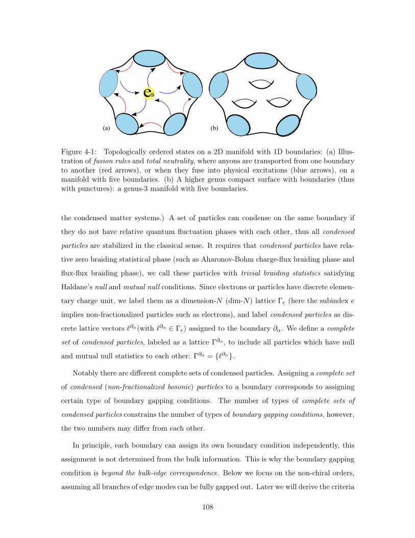
es
(a) (b)
Figure 4-1: Topologically ordered states on a 2D manifold with 1D boundaries: (a) Illus-tration of fusion rules and total neutrality, where anyons are transported from one boundaryto another (red arrows), or when they fuse into physical excitations (blue arrows), on amanifold with five boundaries. (b) A higher genus compact surface with boundaries (thuswith punctures): a genus-3 manifold with five boundaries.
the condensed matter systems.) A set of particles can condense on the same boundary if
they do not have relative quantum fluctuation phases with each other, thus all condensed
particles are stabilized in the classical sense. It requires that condensed particles have rela-
tive zero braiding statistical phase (such as Aharonov-Bohm charge-flux braiding phase and
flux-flux braiding phase), we call these particles with trivial braiding statistics satisfying
Haldane’s null and mutual null conditions. Since electrons or particles have discrete elemen-
tary charge unit, we label them as a dimension-𝑁 (dim-𝑁) lattice Γ𝑒 (here the subindex 𝑒
implies non-fractionalized particles such as electrons), and label condensed particles as dis-
crete lattice vectors ℓ𝜕𝛼(with ℓ𝜕𝛼 ∈ Γ𝑒) assigned to the boundary 𝜕𝛼. We define a complete
set of condensed particles, labeled as a lattice Γ𝜕𝛼 , to include all particles which have null
and mutual null statistics to each other: Γ𝜕𝛼 = {ℓ𝜕𝛼}.
Notably there are different complete sets of condensed particles. Assigning a complete set
of condensed (non-fractionalized bosonic) particles to a boundary corresponds to assigning
certain type of boundary gapping conditions. The number of types of complete sets of
condensed particles constrains the number of types of boundary gapping conditions, however,
the two numbers may differ from each other.
In principle, each boundary can assign its own boundary condition independently, this
assignment is not determined from the bulk information. This is why the boundary gapping
condition is beyond the bulk-edge correspondence. Below we focus on the non-chiral orders,
assuming all branches of edge modes can be fully gapped out. Later we will derive the criteria
108
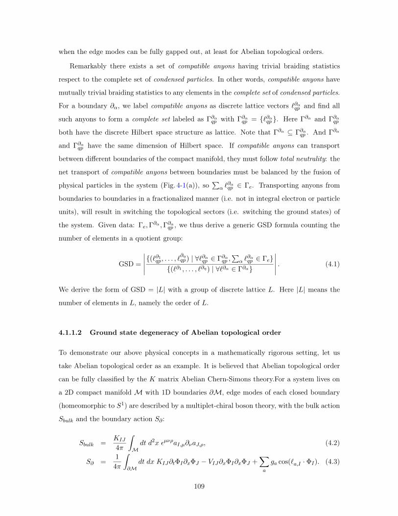
when the edge modes can be fully gapped out, at least for Abelian topological orders.
Remarkably there exists a set of compatible anyons having trivial braiding statistics
respect to the complete set of condensed particles. In other words, compatible anyons have
mutually trivial braiding statistics to any elements in the complete set of condensed particles.
For a boundary 𝜕𝛼, we label compatible anyons as discrete lattice vectors ℓ𝜕𝛼𝑞𝑝 and find all
such anyons to form a complete set labeled as Γ𝜕𝛼𝑞𝑝 with Γ𝜕𝛼𝑞𝑝 = {ℓ𝜕𝛼𝑞𝑝 }. Here Γ𝜕𝛼 and Γ𝜕𝛼𝑞𝑝
both have the discrete Hilbert space structure as lattice. Note that Γ𝜕𝛼 ⊆ Γ𝜕𝛼𝑞𝑝 . And Γ𝜕𝛼
and Γ𝜕𝛼𝑞𝑝 have the same dimension of Hilbert space. If compatible anyons can transport
between different boundaries of the compact manifold, they must follow total neutrality: the
net transport of compatible anyons between boundaries must be balanced by the fusion of
physical particles in the system (Fig. 4-1(a)), so∑
𝛼 ℓ𝜕𝛼𝑞𝑝 ∈ Γ𝑒. Transporting anyons from
boundaries to boundaries in a fractionalized manner (i.e. not in integral electron or particle
units), will result in switching the topological sectors (i.e. switching the ground states) of
the system. Given data: Γ𝑒,Γ𝜕𝛼 ,Γ𝜕𝛼𝑞𝑝 , we thus derive a generic GSD formula counting the
number of elements in a quotient group:
GSD =
{(ℓ𝜕1𝑞𝑝, . . . , ℓ
𝜕𝜂𝑞𝑝) | ∀ℓ𝜕𝛼𝑞𝑝 ∈ Γ𝜕𝛼𝑞𝑝 ,
∑𝛼 ℓ
𝜕𝛼𝑞𝑝 ∈ Γ𝑒}
{(ℓ𝜕1 , . . . , ℓ𝜕𝜂) | ∀ℓ𝜕𝛼 ∈ Γ𝜕𝛼}
. (4.1)
We derive the form of GSD = |𝐿| with a group of discrete lattice 𝐿. Here |𝐿| means the
number of elements in 𝐿, namely the order of 𝐿.
4.1.1.2 Ground state degeneracy of Abelian topological order
To demonstrate our above physical concepts in a mathematically rigorous setting, let us
take Abelian topological order as an example. It is believed that Abelian topological order
can be fully classified by the 𝐾 matrix Abelian Chern-Simons theory.For a system lives on
a 2D compact manifold ℳ with 1D boundaries 𝜕ℳ, edge modes of each closed boundary
(homeomorphic to 𝑆1) are described by a multiplet-chiral boson theory, with the bulk action
𝑆𝑏𝑢𝑙𝑘 and the boundary action 𝑆𝜕 :
𝑆𝑏𝑢𝑙𝑘 =𝐾𝐼𝐽
4𝜋
∫ℳ𝑑𝑡 𝑑2𝑥 𝜖𝜇𝜈𝜌𝑎𝐼,𝜇𝜕𝜈𝑎𝐽,𝜌, (4.2)
𝑆𝜕 =1
4𝜋
∫𝜕ℳ
𝑑𝑡 𝑑𝑥 𝐾𝐼𝐽𝜕𝑡Φ𝐼𝜕𝑥Φ𝐽 − 𝑉𝐼𝐽𝜕𝑥Φ𝐼𝜕𝑥Φ𝐽 +∑𝑎
𝑔𝑎 cos(ℓ𝑎,𝐼 · Φ𝐼). (4.3)
109
Here 𝐾𝐼𝐽 and 𝑉𝐼𝐽 are symmetric integer 𝑁 ×𝑁 matrices, 𝑎𝐼,𝜇 is the 1-form emergent gauge
field’s 𝐼-th component in the multiplet. In terms of edge modes Φ𝐼 with 𝐼 = 1, 2, . . . , 𝑁 ,
this means that there are 𝑁 branches of edge modes. The sine-Gordon term cos(ℓ𝑎,𝐼 ·Φ𝐼) is
derived from a local Hermitian gapping term, 𝑒iℓ𝑎,𝐼 ·Φ𝐼 + 𝑒−iℓ𝑎,𝐼 ·Φ𝐼 ∝ cos(ℓ𝑎,𝐼 · Φ𝐼), where ℓ𝑎
has 𝑁 components under index 𝐼 with integer coefficients.
In this work, we investigate the question how generic 𝑔 cos(ℓ𝑎,𝐼 ·Φ𝐼) terms can fully gap
edge modes, by turning on large 𝑔 coupling interactions. We emphasize that the pertur-
bative relevancy/irrelevancy of cos(ℓ𝑎,𝐼 · Φ𝐼) in the renormalization group (RG) language
is immaterial to our large 𝑔 coupling limit, since there can have energy gap induced by
non-perturbative effects at the strong interaction. Therefore in this work we will include all
possible ℓ𝑎 terms regardless their RG relevancy.
4.1.1.3 Canonical quantization of 𝐾 matrix Abelian Chern-Simons theory edge
modes
In order to understand the energy spectrum or GSD of the edge theory, we study the
‘quantum’ theory, by canonical quantizing the boson field Φ𝐼 . Since Φ𝐼 is the compact
phase of a matter field, its bosonization has zero mode 𝜑0𝐼 and winding momentum 𝑃𝜑𝐽 , in
addition to non-zero modes:
Φ𝐼(𝑥) = 𝜑0𝐼 +𝐾−1𝐼𝐽 𝑃𝜑𝐽
2𝜋
𝐿𝑥+ i
∑��=0
1
𝑛𝛼𝐼,𝑛𝑒
−i𝑛𝑥 2𝜋𝐿 . (4.4)
The periodic boundary size is 𝐿. The conjugate momentum field of Φ𝐼(𝑥) is Π𝐼(𝑥) =
𝛿𝐿𝛿(𝜕𝑡Φ𝐼)
= 12𝜋𝐾𝐼𝐽𝜕𝑥Φ𝐽 . This yields the conjugation relation for zero modes: [𝜑0𝐼 , 𝑃𝜑𝐽 ] = i 𝛿𝐼𝐽 ,
and a generalized Kac-Moody algebra for non-zero modes: [𝛼𝐼,𝑛, 𝛼𝐽,𝑚] = 𝑛𝐾−1𝐼𝐽 𝛿𝑛,−𝑚. We
thus have canonical quantized fields: [Φ𝐼(𝑥1),Π𝐽(𝑥2)] = i 𝛿𝐼𝐽𝛿(𝑥1 − 𝑥2).
4.1.1.4 Braiding Statistics and Boundary Fully Gapping Rules
Let us first intuitively argue the properties of ℓ𝑎 as condensed particles on the edge from
cos(ℓ𝑎,𝐼 · Φ𝐼) of Eq.(4.3). Let us also determine the set of lattice spanned by the discrete
integer ℓ𝑎 vectors: Γ𝜕 = {ℓ𝑎}. We shall name Γ𝜕 as the boundary gapping lattice. Here
𝑎 labels the 𝑎-th vector in Γ𝜕 . From the bulk-edge correspondence, the edge condensed
110
particles labeled by the ℓ𝑎 vector can be mapped to some bulk non-fractionalized particle
excitations ℓ𝑎. It is well-known that the braiding process between two bulk excitations ℓ𝑎
and ℓ𝑏 of Eq.(4.2) causes a mutual-braiding statistical phase term to the whole wavefunction:
exp[i𝜃𝑎𝑏] = exp[i 2𝜋 ℓ𝑎,𝐼𝐾−1𝐼𝐽 ℓ𝑏,𝐽 ]. (4.5)
We will also denote ℓ𝑎,𝐼𝐾−1𝐼𝐽 ℓ𝑏,𝐽 ≡ ℓ𝑇𝑎𝐾
−1ℓ𝑏. On the other hand, the self-exchange process
between two identical excitations ℓ𝑎 of Eq.(4.2) causes a self-braiding statistical phase term
to the whole wavefunction:
exp[i𝜃𝑎𝑎/2] = exp[i𝜋 ℓ𝑎,𝐼𝐾−1𝐼𝐽 ℓ𝑎,𝐽 ]. (4.6)
Without any global symmetry constraint, then any gapping term is allowed. Below we argue
what are the list of properties that the gapping term satisfies to fully gap the edge modes:
(i) Bosonic self-statistics: ∀ℓ𝑎 ∈ Γ𝜕 , ℓ𝑎,𝐼𝐾−1𝐼𝐽 ℓ𝑎,𝐽 ∈ 2Z even integers. This means that the
self-statistics of ℓ𝑎 is bosonic, with a multiple 2𝜋 phase.
(ii) Local: ∀ℓ𝑎, ℓ𝑏 ∈ Γ𝜕 , ℓ𝑎,𝐼𝐾−1𝐼𝐽 ℓ𝑏,𝐽 ∈ Z integers. Winding one ℓ𝑎 around another ℓ𝑏 yields a
bosonic phase, namely a multiple 2𝜋 statistical phase. The bosonic statistics can be viewed
as the local condition.
(iii) Localizing condensate at the classical value without being eliminated by self or mutual
quantum fluctuation: ∀ℓ𝑎, ℓ𝑏 ∈ Γ𝜕 , ℓ𝑎,𝐼𝐾−1𝐼𝐽 ℓ𝑏,𝐽 = 0, so that Zstatistics ∼ exp[i𝜃𝑎𝑏] = 1, the
condensation is stabilized and survives in the classical sense.
(iv) For the cos(ℓ𝑎,𝐼 ·Φ𝐼) term, ℓ𝑎 must be excitations of non-fractionalized particle degrees
of freedom, since it lives on the ‘physical’ boundary, so ℓ𝑎 ∈ Γ𝑒 lattice, where
Γ𝑒 = {∑𝐽
𝑐𝐽𝐾𝐼𝐽 | 𝑐𝐽 ∈ Z}. (4.7)
This rule imposes an integer charge 𝑞𝐼𝐾−1𝐼𝐽 ℓ𝑎,𝐽 in the bulk, and an integer charge 𝑄𝐼 =∫ 𝐿
012𝜋𝜕𝑥Φ𝐼𝑑𝑥 = 𝐾−1
𝐼𝐽 𝑃𝜑𝐽 = 𝐾−1𝐼𝐽 ℓ𝑎,𝐽 for each branch of edge mode 𝐼 on the boundary. Here
𝑞𝐼 is the charge vector coupling to an external field 𝐴𝜇 of gauge or global symmetry, by
adding 𝐴𝜇𝑞𝐼𝐽𝜇𝐼 to the 𝑆𝑏𝑢𝑙𝑘, which corresponds to 𝑞𝐼𝐴𝜇𝜕𝜇Φ𝐼 in the 𝑆𝜕 .
(v) Completeness: we define Γ𝜕 is a complete set, by including every possible term ℓ𝑐 that
has the self null braiding statistics and has the mutually null braiding statistics respect to
111
all the elements ℓ𝑎 ∈ Γ𝜕 . Namely, mathematically we have ∀ℓ𝑐 ∈ Γ𝑒, if ℓ𝑇𝑐 𝐾−1ℓ𝑐 = 0 and
ℓ𝑇𝑐 𝐾−1ℓ𝑎 = 0 for ∀ℓ𝑎 ∈ Γ𝜕 , then ℓ𝑐 ∈ Γ𝜕 must be true. Otherwise Γ𝜕 is not complete.
(vi) The system is non-chiral. We require the same number of left moving modes and right
moving modes to fully gap out the edge modes.
In Sec.4.1.1.5 we will use the bulk braiding statistics property of ℓ𝑎 to determine the
gapped edge stability caused by cos(ℓ𝑎,𝐼 · Φ𝐼) of Eq.(4.3). We leave a derivation that these
properties above are sufficient conditions in Sec.4.1.1.5.
Indeed the above rules (i)(ii)(iii)(iv)(v)(vi) can be simplified to a set of rules which we
call Boundary Fully Gapping Rules.
4.1.1.4.1 Boundary Fully Gapping Rules For an Abelian topological order described
by a bulk Chern-Simons theory of Eq.(4.2) and a boundary theory of Eq.(4.3), we can add
a set of proper interaction terms cos(ℓ𝑎,𝐼 ·Φ𝐼) on the boundary to gap out the edge modes.
We will term that the Boundary Fully Gapping Rules, which summarize all the above rules
(i)(ii)(iii)(iv)(v)(vi) to determine the gapping term ℓ𝑎 ∈ Γ𝜕 . Here ℓ𝑎 is some integer vector,
namely for every component ℓ𝑎,𝐼 ∈ Z. The Γ𝜕 satisfies:
(1) Null and mutual null conditions: ∀ℓ𝑎, ℓ𝑏 ∈ Γ𝜕 , ℓ𝑎,𝐼𝐾−1𝐼𝐽 ℓ𝑏,𝐽 = 0. This implies self statis-
tics and mutual statistics are bosonic, and the excitation is local. Localized fields are not
eliminated by self or mutual quantum fluctuations, so the condensation survives in the clas-
sical sense.
(2) The dimensions of the lattice Γ𝜕 is 𝑁/2, where 𝑁 must be an even integer. Namely, the
Chern-Simons lattice Γ𝜕 assigned to a boundary 𝜕 is spanned by 𝑁/2 linear independent
vectors ℓ𝑎. Mathematically, we write Γ𝜕 = {∑
𝑎=1,2,...,𝑁/2
𝐼𝑎ℓ𝑎,𝐼 | 𝐼𝑎 ∈ Z}.
(3) The system is non-chiral. The signature of 𝐾 matrix (defined as the number of pos-
itive eigenvalues − the number of negative eigenvalues, as 𝑛𝐿 − 𝑛𝑅) must be zero. The
non-chiral edge modes implies a measurable observable, the thermal Hall conductance, to
be zero 𝜅𝑥𝑦 = (𝑛𝐿 − 𝑛𝑅)𝜋2𝑘2𝐵3ℎ 𝑇 = 0. Again, 𝑁 = 𝑛𝐿 + 𝑛𝑅 is even.
There is an extra rule, which will be important later when we try to reproduce the bulk
112
GSD from the boundary GSD:
(4) ‘Physical’ excitation: ℓ𝑎 ∈ Γ𝑒 = {∑
𝐽 𝑐𝐽𝐾𝐼𝐽 | 𝑐𝐽 ∈ Z}. Namely, ℓ𝑎 is an excitation of
non-fractionalized particle degree of freedom, since it lives on the ‘physical’ boundary.
4.1.1.4.2 Comments Here are some comments for the above rules.Since any linear com-
binations of ℓ𝑎 ∈ Γ𝑒 still satisfy (1)(2)(3), we can regard Γ𝜕 as an infinite discrete lattice
group generated by some basis vectors ℓ𝑎.
Physically, the rule (3) excludes some violating examples such as odd rank (denoted as
rk)𝐾 matrix with the chiral central charge 𝑐− = 𝑐𝐿−𝑐𝑅 = 0 or the thermal Hall conductance
𝜅𝑥𝑦 = 0, which universally has gapless chiral edge modes. For instance, the dim-1 boundary
gapping lattice: {𝑛(𝐴,𝐵,𝐶) | 𝑛 ∈ Z} of 𝐾3×3 = diag(1, 1,−1), with 𝐴2 + 𝐵2 − 𝐶2 = 0,
satisfies the rules (1)(2), but cannot fully gap out chiral edge modes.
4.1.1.5 Hamiltonian and Energy Gap
Here we will justify the Boundary Fully Gapping Rules in Sec.4.1.1.4 is sufficient to fully
gap the edge modes. Our approach is to explicitly calculate the mass gap for the zero energy
mode and its higher excitations. We will show that if the Boundary Fully Gapping Rules
hold, there are stable mass gaps for all edge modes.
We consider the even-rank symmetric 𝐾 matrix, satisfying the rule (3), so the non-chiral
system with even number of edge modes can potentially be gappable.
To determine the mass gap of the boundary modes, and to examine the gap in the
large system size limit 𝐿 → ∞, we will take the large 𝑔 coupling limit of the Hamilto-
nian: −𝑔𝑎∫ 𝐿0 𝑑𝑥 cos(ℓ𝑎,𝐼 · Φ𝐼) →
12𝑔𝑎(ℓ𝑎,𝐼 · Φ𝐼)
2𝐿. By exactly diagonalizing the quadratic
Hamiltonian,
𝐻 ≃ (
∫ 𝐿
0𝑑𝑥 𝑉𝐼𝐽𝜕𝑥Φ𝐼𝜕𝑥Φ𝐽) +
1
2
∑𝑎
𝑔𝑎(ℓ𝑎,𝐼 · Φ𝐼)2𝐿+ . . . , (4.8)
with a Φ mode expansion Eq.(4.4), we obtain the energy spectra from its eigenvalues. We
realize that:
∙ Remark 1: If we include all the interaction terms allowed by Boundary Full Gapping
113
Rules, we can turn on the energy gap of zero modes (𝑛 = 0) as well as the Fourier modes
(non-zero modes 𝑛 = 0). The energy spectrum is in the form of
𝐸𝑛 =(√
Δ2 +#(2𝜋𝑛
𝐿)2 + . . .
), (4.9)
where Δ is the mass gap. Here # means some numerical factor. We emphasize the energy
of Fourier modes (𝑛 = 0) behaves towards zero modes at long wave-length low energy limit
(𝐿 → ∞). Such spectra become continuous at 𝐿 → ∞ limit, which is the expected energy
behavior.
∙ Remark 2: If we include the incompatible interaction term, e.g. ℓ𝑎 and ℓ′ where
ℓ𝑇𝑎𝐾−1ℓ′ = 0, while the interaction terms contain
∑𝑎 𝑔𝑎 cos(ℓ𝑎 ·Φ)+ 𝑔′ cos(ℓ′ ·Φ), we obtain
the unstable energy spectrum:
𝐸𝑛 =(√
Δ2𝑚 +#(
2𝜋𝑛
𝐿)2 +
∑𝑎
#𝑔𝑎 𝑔′(𝐿
𝑛)2 + . . .+ . . .
). (4.10)
The energy spectra exhibits an instability of the system, because at low energy limit (𝐿→
∞), the spectra become discontinuous (from 𝑛 = 0 to 𝑛 = 0) and jump to infinity as long
as there are incompatible cosine terms (i.e. 𝑔𝑎 · 𝑔′ = 0). The dangerous behavior of (𝐿/𝑛)2
implies the quadratic expansion analysis may not describe the full physics. In that case,
the dangerous behavior invalidates localizing of Φ field at a minimum. This invalidates the
energy gap, and the unstable system potentially seeks to become gapless phases.
∙ Remark 3: We provide an alternative way to study the energy gap stability. We include
the full cosine interaction term for the lowest energy states, namely the zero and winding
modes:
cos(ℓ𝑎,𝐼 · Φ𝐼)→ cos(ℓ𝑎,𝐼 · (𝜑0𝐼 +𝐾−1𝐼𝐽 𝑃𝜑𝐽
2𝜋
𝐿𝑥)). (4.11)
The stability of the energy gap can be understood from under what criteria we can safely
expand the cosine term to extract the leading quadratic terms by only keeping the zero
modes, namely cos(ℓ𝑎,𝐼 · Φ𝐼) ≃ 1 − 12(ℓ𝑎,𝐼 · 𝜑0𝐼)
2 + . . . . The naive reason is the following:
if one does not decouple the winding mode 𝑃𝜑𝐽 term, there is a complicated 𝑥 dependence
in 𝑃𝜑𝐽2𝜋𝐿 𝑥 along the 𝑥 integration. The non-commuting algebra [𝜑0𝐼 , 𝑃𝜑𝐽 ] = i𝛿𝐼𝐽 results in
the challenge for this cosine expansion. This challenge can be resolved by requiring ℓ𝑎,𝐼𝜑0𝐼
114
and ℓ𝑎,𝐼′𝐾−1𝐼′𝐽𝑃𝜑𝐽 commute in Eq.(4.11),
[ℓ𝑎,𝐼𝜑0𝐼 , ℓ𝑎,𝐼′𝐾−1𝐼′𝐽𝑃𝜑𝐽 ] = ℓ𝑎,𝐼𝐾
−1𝐼′𝐽ℓ𝑎,𝐼′ (i𝛿𝐼𝐽) = (ℓ𝑎,𝐽𝐾
−1𝐼′𝐽ℓ𝑎,𝐼′)(i) = 0. (4.12)
In fact this is the Boundary Full Gapping Rule (1) for the self null statistics — the triv-
ial self statistics rule among the interaction gapping terms. We can interpret that there
is no quantum fluctuation destabilize the semi-classical particle condensation. With this
commuting criterion, we can safely expand Eq.(4.11) by the trigonometric identity as
cos(ℓ𝑎,𝐼𝜑0𝐼) cos(ℓ𝑎,𝐼𝐾−1𝐼𝐽 𝑃𝜑𝐽
2𝜋
𝐿𝑥)− sin(ℓ𝑎,𝐼𝜑0𝐼) sin(ℓ𝑎,𝐼𝐾
−1𝐼𝐽 𝑃𝜑𝐽
2𝜋
𝐿𝑥). (4.13)
Then we integrate over the circumference 𝐿. First, we notice that ℓ𝑎,𝐼𝐾−1𝐼𝐽 𝑃𝜑𝐽 takes integer
values due to ℓ𝑎,𝐼 ∈ Γ𝑒 and 𝑃𝜑𝐽 ∈ Z. Further we notice that due to the periodicity of
both cos(. . . 𝑥) and sin(. . . 𝑥) in the region [0, 𝐿), so both 𝑥-integrations over [0, 𝐿) vanish.
However, the exception is ℓ𝑎,𝐼 ·𝐾−1𝐼𝐽 𝑃𝜑𝐽 = 0, then cos(ℓ𝑎,𝐼𝐾
−1𝐼𝐽 𝑃𝜑𝐽
2𝜋𝐿 𝑥) = 1. We derive:
𝑔𝑎
∫ 𝐿
0𝑑𝑥 Eq.(4.11) = 𝑔𝑎𝐿 cos(ℓ𝑎,𝐼 · 𝜑0𝐼)𝛿(ℓ𝑎,𝐼 ·𝐾−1
𝐼𝐽 𝑃𝜑𝐽,0). (4.14)
The Kronecker-delta function 𝛿(ℓ𝑎,𝐼 ·𝐾−1𝐼𝐽 𝑃𝜑𝐽
,0) = 1 indicates that there is a nonzero contribu-
tion if and only if ℓ𝑎,𝐼 ·𝐾−1𝐼𝐽 𝑃𝜑𝐽 = 0.
So far we have shown that when the self-null braiding statistics ℓ𝑇𝐾−1ℓ = 0 is true, we
have the desired cosine potential expansion via the zero mode quadratic expansion at the
large 𝑔𝑎 coupling, 𝑔𝑎∫ 𝐿0 𝑑𝑥 cos(ℓ𝑎,𝐼 ·Φ𝐼) ≃ −𝑔𝑎𝐿
12(ℓ𝑎,𝐼 ·𝜑0𝐼)
2+ . . . . If we include not enough
gapping terms (less than 𝑁/2 terms), we cannot fully gap all edge modes. On the other
hand, if we include more than the Boundary Full Gapping Rules (more than 𝑁/2 terms with
incompatible terms), there is a disastrous behavior in the spectrum (see Remark 2). We
need to include the mutual-null braiding statistics ℓ𝑇𝑎𝐾−1ℓ𝑏 = 0 so that the energy gap is
stable.
The quadratic Hamiltonian includes both the kinetic and the leading-order of the po-
tential terms:(2𝜋)2
4𝜋𝐿𝑉𝐼𝐽𝐾
−1𝐼𝑙1𝐾−1𝐽𝑙2𝑃𝜑𝑙1𝑃𝜑𝑙2 +
∑𝑎
𝑔𝑎𝐿1
2(ℓ𝑎,𝐼 · 𝜑0𝐼)2 (4.15)
By solving the quadratic simple harmonic oscillators, we can show the nonzero energy gaps
115
of zero modes. The mass matrix can be properly diagonalized, since there are only conjugate
variables 𝜑0𝐼 , 𝑃𝜑,𝐽 in the quadratic order. The energy gap is of the order one finite gap,
independent of the system size 𝐿,
Δ ≃ 𝑂(√2𝜋 𝑔𝑎ℓ𝑎,𝑙1ℓ𝑎,𝑙2𝑉𝐼𝐽𝐾
−1𝐼𝑙1𝐾−1𝐽𝑙2
). (4.16)
In the diagonalized basis of the Hamiltonian Eq.(4.15), the energy gap Δ𝐼 has the component
𝐼-dependence.
More precisely, we find the dimension of independent gapping terms Γ𝜕 = {ℓ𝑎} must
be 𝑁/2, namely satisfying Boundary Full Gapping Rules (2). The number of left and right
moving modes must be the same, namely satisfying the non-chiral criterion in Boundary
Full Gapping Rules (3). To summarize, by calculating the stability of energy gap, we have
thus demonstrated that the Boundary Full Gapping Rules (1)(2)(3) are sufficient to ensure
that the energy gap is stable at large 𝑔 coupling.
Due to the periodicity of 𝜑0 , its conjugate variable 𝑃𝜑 forms a discrete quantized lat-
tice. This is consistent with the discrete Hilbert space of the ground states, forming the
Chern-Simons quantized lattice detailed in Sec.4.1.1.6. We will apply this idea to count the
ground state degeneracy of the Chern-Simons theory on a closed manifold or a compact
manifold with gapped boundaries. The Boundary Full Gapping Rules (4) will be required
for computing the boundary GSD and the bulk GSD.
4.1.1.6 Hilbert Space
Since 𝜑0 is periodic, so 𝑃𝜑 forms a discrete lattice. We now impose the rule (4), so cos(ℓ𝑎,𝐼 ·
𝜑0𝐼) are hopping terms along condensed particle vector ℓ𝑎,𝐼 in sublattice of Γ𝑒 in the 𝑃𝜑
lattice. We can show that rule (4) is essential to derive the bulk GSD by computing the
boundary GSD under gluing the boundaries.
Let 𝑃 𝑞𝑝𝜑 represents some compatible anyon ℓ𝑞𝑝 which is mutual null to condensed particles
ℓ by ℓ𝑇𝐾−1𝑃 𝑞𝑝𝜑 = ℓ𝑇𝐾−1ℓ𝑞𝑝 = 0. By the rule (1), thus it means that the compatible anyon
ℓ𝑞𝑝 parallels along some ℓ vector. However, ℓ𝑞𝑝 lives on the quasiparticle lattice, i.e. the unit
integer lattice of the 𝑃𝜑 lattice. So ℓ𝑞𝑝 is parametrized by 1| gcd(ℓ𝑎)|
ℓ𝑎,𝐽 , with the greatest
common divisor defined as | gcd(ℓ𝑎)| ≡ gcd(|ℓ𝑎,1|, |ℓ𝑎,2|, . . . , |ℓ𝑎,𝑁 |).
Now let us consider the Hilbert space of ground states in terms of 𝑃𝜑 lattice. For the
116
Hilbert space of ground states, we will neglect the kinetic term 𝐻𝑘𝑖𝑛 = (2𝜋)2
4𝜋𝐿 𝑉𝐼𝐽𝐾−1𝐼𝑙1𝐾
−1𝐽𝑙2𝑃𝜑𝑙1
𝑃𝜑𝑙2 of the order 𝑂(1/𝐿) as 𝐿→∞. Recall we label the 𝛼-th boundary of a compact spatial
manifold with 𝜂 punctures as 𝜕𝛼, where 𝛼 = 1, . . . , 𝜂. Note that 𝑎 is the index for 𝑎-th ℓ
vector: ℓ𝜕𝛼𝑎 ∈ Γ𝜕𝛼 . If we choose the proper basis ℓ vector, based on the rule (2), we have
𝑎 = 1, . . . , 𝑁/2. For the 𝛼-th boundary 𝜕𝛼, a complete set of condensed particles forms the
boundary gapping lattice:
Γ𝜕𝛼 = {∑
𝑎=1,...,𝑁/2
𝐼𝜕𝛼𝑎 ℓ𝜕𝛼𝑎,𝐼 | 𝐼𝜕𝛼𝑎 ∈ Z}. (4.17)
Recall 𝐼 is the 𝐼-th branch of 𝐾𝑁×𝑁 matrix, 𝐼 = 1, . . . , 𝑁 .
A complete set of compatible anyon vectors ℓ𝑞𝑝 forms the Hilbert space of the winding
mode 𝑃𝜑 lattice:
Γ𝜕𝛼𝑞𝑝 = {ℓ𝜕𝛼𝑞𝑝,𝐼} = {∑
𝑎=1,...,𝑁/2
𝑗𝜕𝛼𝑎ℓ𝜕𝛼𝑎,𝐼
| gcd(ℓ𝜕𝛼𝑎 )|| 𝑗𝜕𝛼𝑎 ∈ Z}, (4.18)
or simply the anyon hopping lattice. Note Γ𝜕𝛼 , Γ𝜕𝛼𝑞𝑝 are infinite Abelian discrete lattice group.
Anyon fusion rules and the total neutrality condition essentially means the bulk physical
charge excitation can fuse from or split to multiple anyon charges. The rules constrain the
set of 𝑗𝜕𝛼𝑎 values to be limited on the Γ𝑒 lattice.
To be more precise mathematically, the anyon fusion rules and the total neutrality con-
dition constrain the direct sum of the anyon hopping lattice Γ𝜕𝛼𝑞𝑝 , with 𝛼 = 1, . . . , 𝜂 over all 𝜂
boundaries, must be on the Γ𝑒 lattice. We define such a constrained anyon hopping lattice
as 𝐿𝑞𝑝⋂ 𝑒:
𝐿𝑞𝑝⋂𝑒 ≡ {
𝜂⨁𝛼=1
𝑁/2∑𝑎=1
𝑗𝜕𝛼𝑎ℓ𝜕𝛼𝑎,𝐼
| gcd(ℓ𝜕𝛼𝑎 )|| ∀𝑗𝜕𝛼𝑎 ∈ Z, ∃ 𝑐𝐽 ∈ Z,
𝜂∑𝛼=1
𝑁/2∑𝑎=1
𝑗𝜕𝛼𝑎ℓ𝜕𝛼𝑎,𝐼
| gcd(ℓ𝜕𝛼𝑎 )|=
𝑁∑𝐽=1
𝑐𝐽𝐾𝐼𝐽}. (4.19)
4.1.1.6.1 Number of types of boundary gapping conditions As we exactly solve
the number of types of boundary gapping lattices, we find that for rk(𝐾) = 2, we obtain
two boundary gapping lattices. However, when we consider boundary gapping conditions,
117
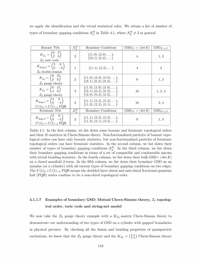
we apply the identification and the trivial statistical rules. We obtain a list of number of
types of boundary gapping conditions 𝒩 𝜕𝑔 in Table 4.1, where 𝒩 𝜕
𝑔 = 2 in general.
Bosonic TOs 𝒩 𝜕𝑔 Boundary Conditions GSD𝑇 2 = |det𝐾| GSD𝑆1×𝐼1
𝐾𝑍2=
(0 22 0
)𝑍2 toric code
2 {(1, 0), (2, 0), . . . },{(0, 1), (0, 2), . . . } 4 1, 2
𝐾diag,2 =
(2 00 −2
)𝑍2 double-semion
1 {(1, 1), (2, 2), . . . } 4 2
𝐾𝑍3=
(0 33 0
)𝑍3 gauge theory
2 {(1, 0), (2, 0), (3, 0), . . . },{(0, 1), (0, 2), (0, 3), . . . } 9 1, 3
𝐾𝑍4=
(0 44 0
)𝑍4 gauge theory
3{(1, 0), (2, 0), (3, 0), . . . },{(0, 1), (0, 2), (0, 3), . . . },{(2, 0), (0, 2), (2, 2), . . . }
16 1, 2, 4
𝐾diag,4 =
(4 00 −4
)𝑈(1)4 × 𝑈(1)−4 FQH
2 {(1, 1), (2, 2), (3, 3), . . . },{(1, 3), (2, 2), (3, 1), . . . } 16 2, 4
Fermionic TOs 𝒩 𝜕𝑔 Boundary Conditions GSD𝑇 2 = |det𝐾| GSD𝑆1×𝐼1
𝐾diag,3 =
(3 00 −3
)𝑈(1)3 × 𝑈(1)−3 FQH
2 {(1, 1), (2, 2), (3, 3), . . . },{(1, 2), (2, 1), (3, 3), . . . } 9 1, 3
Table 4.1: In the first column, we list down some bosonic and fermionic topological ordersand their 𝐾-matrices in Chern-Simons theory. Non-fractionalized particles of bosonic topo-logical orders can have only bosonic statistics, but non-fractionalized particles of fermionictopological orders can have fermionic statistics. In the second column, we list down theirnumber of types of boundary gapping conditions 𝒩 𝜕
𝑔 . In the third column, we list downtheir boundary gapping conditions in terms of a set of compatible and condensable anyonswith trivial braiding statistics. In the fourth column, we list down their bulk GSD= | det𝐾|on a closed manifold 2-torus. In the fifth column, we list down their boundary GSD on anannulus (or a cylinder) with all various types of boundary gapping conditions on two edges.The 𝑈(1)𝑘×𝑈(1)−𝑘 FQH means the doubled layer chiral and anti-chiral fractional quantumhall (FQH) states combine to be a non-chiral topological order.
4.1.1.7 Examples of boundary GSD: Mutual Chern-Simons theory, 𝑍𝑘 topolog-
ical order, toric code and string-net model
We now take the 𝑍𝑘 gauge theory example with a 𝐾𝑍𝑘-matrix Chern-Simons theory to
demonstrate our understanding of two types of GSD on a cylinder with gapped boundaries
in physical pictures. By checking all the fusion and braiding properties of quasiparticle
excitations, we know that the 𝑍𝑘 gauge theory and the 𝐾𝑍𝑘=
(0 𝑘𝑘 0
)Chern-Simons theory
118
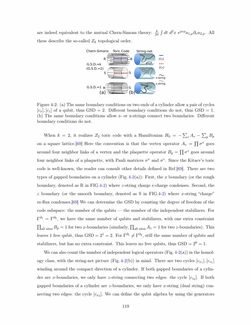
are indeed equivalent to the mutual Chern-Simons theory: 𝑘2𝜋
∫𝑑𝑡 𝑑2𝑥 𝜖𝜇𝜈𝜌𝑎1,𝜇𝜕𝜈𝑎2,𝜌. All
these describe the so-called 𝑍𝑘 topological order.
(a) (b)
G.S.D.=k
G.S.D.=1
Toric Code String-netChern-Simons
(G.S.D.=2)
RR
R S
S S
[Cx]
[Cz]
z-string
x-string
Figure 4-2: (a) The same boundary conditions on two ends of a cylinder allow a pair of cycles[𝑐𝑥], [𝑐𝑧] of a qubit, thus GSD = 2. Different boundary conditions do not, thus GSD = 1.(b) The same boundary conditions allow z- or x-strings connect two boundaries. Differentboundary conditions do not.
When 𝑘 = 2, it realizes 𝑍2 toric code with a Hamiltonian 𝐻0 = −∑
𝑣 𝐴𝑣 −∑
𝑝𝐵𝑝
on a square lattice.[69] Here the convention is that the vertex operator 𝐴𝑣 =∏𝜎𝑥 goes
around four neighbor links of a vertex and the plaquette operator 𝐵𝑝 =∏𝜎𝑧 goes around
four neighbor links of a plaquette, with Pauli matrices 𝜎𝑥 and 𝜎𝑧. Since the Kitaev’s toric
code is well-known, the reader can consult other details defined in Ref.[69]. There are two
types of gapped boundaries on a cylinder (Fig. 4-2(a)): First, the 𝑥 boundary (or the rough
boundary, denoted as R in FIG.4-2) where 𝑧-string charge 𝑒-charge condenses. Second, the
𝑧 boundary (or the smooth boundary, denoted as S in FIG.4-2) where 𝑥-string “charge”
𝑚-flux condenses.[69] We can determine the GSD by counting the degree of freedom of the
code subspace: the number of the qubits — the number of the independent stabilizers. For
Γ𝜕1 = Γ𝜕2 , we have the same number of qubits and stabilizers, with one extra constraint∏all sites𝐵𝑝 = 1 for two 𝑥-boundaries (similarly,
∏all sites𝐴𝑣 = 1 for two 𝑧-boundaries). This
leaves 1 free qubit, thus GSD = 21 = 2. For Γ𝜕1 = Γ𝜕2 , still the same number of qubits and
stabilizers, but has no extra constraint. This leaves no free qubits, thus GSD = 20 = 1.
We can also count the number of independent logical operators (Fig. 4-2(a)) in the homol-
ogy class, with the string-net picture (Fig. 4-2(b)) in mind. There are two cycles [𝑐𝑥1 ], [𝑐𝑧1 ]
winding around the compact direction of a cylinder. If both gapped boundaries of a cylin-
der are 𝑥-boundaries, we only have 𝑧-string connecting two edges: the cycle [𝑐𝑧2 ]. If both
gapped boundaries of a cylinder are 𝑧-boundaries, we only have 𝑥-string (dual string) con-
necting two edges: the cycle [𝑐𝑥2 ]. We can define the qubit algebra by using the generators
119
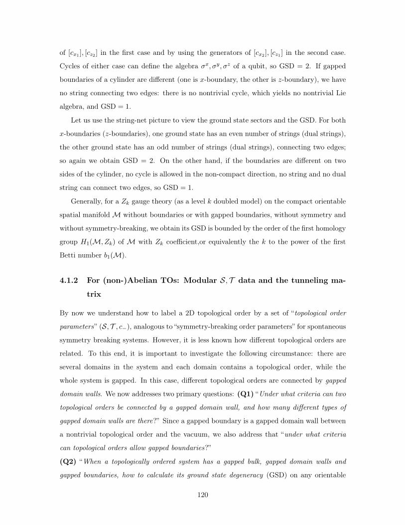
of [𝑐𝑥1 ], [𝑐𝑧2 ] in the first case and by using the generators of [𝑐𝑥2 ], [𝑐𝑧1 ] in the second case.
Cycles of either case can define the algebra 𝜎𝑥, 𝜎𝑦, 𝜎𝑧 of a qubit, so GSD = 2. If gapped
boundaries of a cylinder are different (one is 𝑥-boundary, the other is 𝑧-boundary), we have
no string connecting two edges: there is no nontrivial cycle, which yields no nontrivial Lie
algebra, and GSD = 1.
Let us use the string-net picture to view the ground state sectors and the GSD. For both
𝑥-boundaries (𝑧-boundaries), one ground state has an even number of strings (dual strings),
the other ground state has an odd number of strings (dual strings), connecting two edges;
so again we obtain GSD = 2. On the other hand, if the boundaries are different on two
sides of the cylinder, no cycle is allowed in the non-compact direction, no string and no dual
string can connect two edges, so GSD = 1.
Generally, for a 𝑍𝑘 gauge theory (as a level 𝑘 doubled model) on the compact orientable
spatial manifoldℳ without boundaries or with gapped boundaries, without symmetry and
without symmetry-breaking, we obtain its GSD is bounded by the order of the first homology
group 𝐻1(ℳ, 𝑍𝑘) of ℳ with 𝑍𝑘 coefficient,or equivalently the 𝑘 to the power of the first
Betti number 𝑏1(ℳ).
4.1.2 For (non-)Abelian TOs: Modular 𝒮, 𝒯 data and the tunneling ma-
trix
By now we understand how to label a 2D topological order by a set of “topological order
parameters” (𝒮, 𝒯 , 𝑐−), analogous to “symmetry-breaking order parameters” for spontaneous
symmetry breaking systems. However, it is less known how different topological orders are
related. To this end, it is important to investigate the following circumstance: there are
several domains in the system and each domain contains a topological order, while the
whole system is gapped. In this case, different topological orders are connected by gapped
domain walls. We now addresses two primary questions: (Q1) “Under what criteria can two
topological orders be connected by a gapped domain wall, and how many different types of
gapped domain walls are there?” Since a gapped boundary is a gapped domain wall between
a nontrivial topological order and the vacuum, we also address that “under what criteria
can topological orders allow gapped boundaries?”
(Q2) “When a topologically ordered system has a gapped bulk, gapped domain walls and
gapped boundaries, how to calculate its ground state degeneracy (GSD) on any orientable
120
manifold?”
We have partially achieved results from Abelian TOs and GSD with gapped boundaries.
Here we will take another approach to generalize our theory to non-Abelian TOs and GSD
with gapped domain walls.
4.1.2.1 Main result
Consider two topological orders, Phases𝐴 and𝐵, described by (𝒮𝐴, 𝒯 𝐴, 𝑐𝐴−) and (𝒮𝐵, 𝒯 𝐵, 𝑐𝐵−).
Suppose there are 𝑁 and 𝑀 types of anyons in Phase 𝐴 and Phase 𝐵, then the ranks of
their modular matrices are 𝑁 and 𝑀 respectively. If 𝐴 and 𝐵 are connected by a gapped
domain wall, firstly their central charges must be the same 𝑐𝐴− = 𝑐𝐵−. Next we find that the
domain wall can be labeled by a 𝑀 ×𝑁 tunneling matrix 𝒲 whose entries are fusion-space
dimensions 𝒲𝑖𝑎 satisfying the commuting condition (4.21), and the stable condition (4.22):
𝒲𝑖𝑎 ∈ Z, (4.20)
𝒮𝐵𝒲 =𝒲𝒮𝐴, 𝒯 𝐵𝒲 =𝒲𝒯 𝐴, (4.21)
𝒲𝑖𝑎𝒲𝑗𝑏 ≤∑𝑘𝑐
(𝒩𝐵)𝑘𝑖𝑗𝒲𝑘𝑐(𝒩𝐴)𝑐𝑎𝑏 . (4.22)
Z denotes the set of non-negative integers. 𝑎, 𝑏, 𝑐, . . . and 𝑖, 𝑗, 𝑘, . . . are anyon indices for
Phases 𝐴,𝐵. (𝒩𝐴)𝑐𝑎𝑏 and (𝒩𝐵)𝑘𝑖𝑗 are fusion tensors of Phases 𝐴,𝐵.
(4.20)(4.21)(4.22) is a set of necessary conditions a gapped domain wall must satisfy, i.e.,
if there is no non-zero solution of 𝒲, the domain wall must be gapless. We conjecture that
they are also sufficient for a gapped domain wall to exist. In the examples studied, 𝒲 are
in one-to-one correspondence with gapped domain walls. However, for some complicated
examples, a 𝒲 matrix may correspond to more than one type of gapped domain wall. This
indicates that some additional data are needed to completely classify gapped domain walls.
As a first application of our result, we give a general method to compute the GSD in
the presence of gapped domain walls on any orientable 2D surface. A simple case is the
GSD on a disk drilled with two holes (equivalently a sphere with 3 circular boundaries, see
Fig. 4-5(c)). The gapped boundaries are labeled by three vectors (one-row or one-column
matrices) 𝒲(1),𝒲(2),𝒲(3). The GSD is∑
𝑖𝑗𝑘𝒲(1)𝑖1 𝒲
(2)𝑗1 𝒩 𝑘
𝑖𝑗𝒲(3)1𝑘 .
For gapped boundaries, our criteria can be understood via dimension reduction, i.e.,
121
shrinking a 1D gapped boundary𝒲 to a (composite 1) anyon 𝑞𝒲 = ⊕𝑎𝒲1𝑎𝑎. If the system is
on a 2D surface𝑀2 drilled with 𝑛 gapped boundaries𝒲(1), . . . ,𝒲(𝑛), then the GSD is the di-
mension of the fusion space with anyons 𝑞𝒲(1) , . . . , 𝑞𝒲(𝑛) , GSD = dim[𝒱(𝑀2, 𝑞𝒲(1) , . . . , 𝑞𝒲(𝑛))].
Since gapped domain walls talk to each other through long-range entanglement, the
GSD with domain walls reveals more physics than that without domain walls. We foresee
its practicality in experiments, since we can read even more physics by putting the system
on open surfaces with gapped domain walls. Below we shall properly introduce 𝒮, 𝒯 and 𝒲
matrices.
4.1.2.2 Modular 𝒮, 𝒯 matrices
𝒮 and 𝒯 are unitary matrices indexed by anyon types {1, 𝑎, 𝑏, 𝑐, . . . }. 1 labels the trivial
anyon type. The anti-quasiparticle of 𝑎 is denoted by 𝑎*.
𝒯 describes the self statistics. It is diagonal 𝒯𝑎𝑏 = e i𝜃𝑎𝛿𝑎𝑏, where e i𝜃𝑎 is the phase
factor when exchanging two anyons 𝑎. For the trivial type, 𝒯11 = e i𝜃1 = 1. 𝒮 describes the
mutual statistics. 𝒮𝑎𝑏 is the amplitude of the following process with proper normalization
factors: first create a pair of 𝑎𝑎* and a pair of 𝑏𝑏*, then braid 𝑎 around 𝑏, and finally
annihilate the two pairs. 𝒮 is symmetric, 𝒮𝑎𝑏 = 𝒮𝑏𝑎. If 𝑏 = 1, the process is just creation
and annihilation, and 𝒮𝑎1 > 0. 𝒮 and 𝒯 form a projective representation of the modular
group: 𝒮4 = 𝐼, (𝒮𝒯 )3 = e2𝜋 i𝑐−/8𝒮2, where 𝐼 denotes the identity matrix.
The anti-quasiparticle can be read from 𝒮2, (𝒮2)𝑎𝑏 = 𝛿𝑎*𝑏. The fusion tensor 𝒩 𝑐𝑎𝑏 can be
calculated via the Verlinde formula:
𝒩 𝑐𝑎𝑏 =
∑𝑚
𝒮𝑎𝑚𝒮𝑏𝑚𝒮𝑐𝑚𝒮1𝑚
∈ Z. (4.23)
Gapped domain walls– Below we demonstrate the physical meanings of the gapped do-
main wall conditions (4.20)(4.21)(4.22). First we put Phase 𝐴 and Phase 𝐵 on a sphere
𝑆2, separated by a gapped domain wall. Note that there can be many types of domain
walls separating the same pair of phases 𝐴 and 𝐵. What data characterize those dif-
ferent types of domain walls? We fix the domain wall type, labeled by 𝑊 , and trap
an anyon 𝑎* in Phase 𝐴, an anyon 𝑖 in Phase 𝐵 and. This configuration is denoted by
(𝑆2, 𝑖,𝑊, 𝑎*). The states with such a configuration may be degenerate and the degenerate
1The concepts of trapping anyons, composite anyon types and fusion spaces are discussed in [98]
122
subspace is the fusion space 𝒱(𝑆2, 𝑖,𝑊, 𝑎*). Here we propose using the fusion-space dimen-
sions 𝒲𝑖𝑎 ≡ dim[𝒱(𝑆2, 𝑖,𝑊, 𝑎*)] ∈ Z to characterize the gapped domain wall 𝑊 . Below we
will replace the abstract label 𝑊 by the concrete data 𝒲.
There are non-local operators 𝑂𝑊,𝑖𝑎* that create a pair 𝑎𝑎* in Phase 𝐴, and then tunnel
𝑎 through the domain wall to an anyon 𝑖 in Phase 𝐵, 𝑂𝑊,𝑖𝑎* |𝜓𝑆2,𝑊 ⟩ ∈ 𝒱(𝑆2, 𝑖,𝑊, 𝑎*),
where |𝜓𝑆2,𝑊 ⟩ is the ground state. Since we care about the fusion states rather than
the operators themselves, we would take the equivalent class [𝑂𝑊,𝑖𝑎* ] = {𝑈𝑊,𝑖𝑎* |(𝑂𝑊,𝑖𝑎* −
𝑈𝑊,𝑖𝑎*)|𝜓𝑆2,𝑊 ⟩ = 0}. We call [𝑂𝑊,𝑖𝑎* ] as tunneling channels, which correspond to fusion
states in 𝒱(𝑆2, 𝑖,𝑊, 𝑎*). Therefore, the fusion space dimension 𝒲𝑖𝑎 is the number of lin-
early independent tunneling channels. So we also refer to 𝒲 as the “tunneling matrix.”
We can compute the dimension of the fusion space 𝒱(𝑆2, 𝑖,𝑊, 𝑎*) by first creating a
pair 𝑎𝑎* in Phase 𝐴, then tunneling 𝑎 through the domain wall. In the channel where the
tunneling does not leave any topological quasiparticle on the domain wall, 𝑎 in Phase 𝐴 will
become a composite anyon 𝑞𝒲,𝑎 = ⊕𝑖𝒲𝑖𝑎𝑖 in Phase 𝐵. Thus the fusion-space dimension
𝒲𝑖𝑎 is also the number of tunneling channels from, 𝑎 of Phase A, to, 𝑖 of Phase 𝐵. So we
also refer to 𝒲 as the “tunneling matrix.”
The commuting condition (4.21) dictates the consistency of anyon statistics in presence
of gapped domain walls. Since modular 𝒮, 𝒯 matrices encode the anyon statistics, we require
that 𝒲 should commute with them as (4.21): 𝒮𝐵𝒲 =𝒲𝒮𝐴, 𝒯 𝐵𝒲 =𝒲𝒯 𝐴.
We may as well create a pair 𝑖𝑖* in Phase 𝐵 and tunnel 𝑖* to 𝑎*. 𝒲† describes such
tunneling in the opposite direction (i.e., 𝒲 : 𝐴 → 𝐵, 𝒲† : 𝐵 → 𝐴). 𝒲† and 𝒲 contains
the same physical data. To be consistent, tunneling 𝑖* to 𝑎* should give the same fusion-
space dimension, (𝒲†)𝑎*𝑖* = 𝒲𝑖*𝑎* = 𝒲𝑖𝑎. This is guaranteed by 𝒲(𝒮𝐴)2 = (𝒮𝐵)2𝒲 and
(𝒮2)𝑎𝑏 = 𝛿𝑎*𝑏.
The fusion spaces with four anyons further provide us consistence conditions of𝒲. To see
this, first notice that there are generalised tunneling channels, [𝑂𝑊,𝑖𝑎*,𝑥], which, in addition
to tunneling 𝑎 to 𝑖, also create quasiparticle 𝑥 on the domain wall. If we combine the
tunneling channels [𝑂𝑊,𝑖𝑎*,𝑥] and [𝑂𝑊,𝑗𝑏*,𝑥* ], we can create fusion states with a domain wall
𝑊 and four anyons 𝑖, 𝑗, 𝑎*, 𝑏*, as Fig. 4-3(a). In other words, [𝑂𝑊,𝑖𝑎*,𝑥𝑂𝑊,𝑗𝑏*,𝑥* ] form a basis
of the fusion space 𝒱(𝑆2, 𝑖, 𝑗,𝑊, 𝑎*, 𝑏*). Let 𝒦𝑥𝑖𝑎 denote the number of tunneling channels
[𝑂𝑊,𝑖𝑎*,𝑥], and we know that dim𝒱(𝑆2, 𝑖, 𝑗,𝑊, 𝑎*, 𝑏*) =∑
𝑥𝒦𝑥𝑖𝑎𝒦𝑥*𝑗𝑏 . However, the tunneling
process as Fig. 4-3(b), i.e., fusing 𝑎, 𝑏 to 𝑐, using [𝑂𝑊,𝑘𝑐* ] to tunnel 𝑐 to 𝑘 and splitting 𝑘 to
123
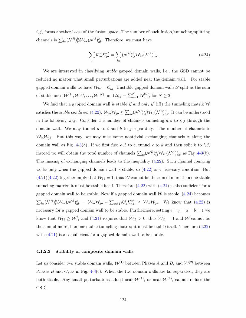
𝑖, 𝑗, forms another basis of the fusion space. The number of such fusion/tunneling/splitting
channels is∑
𝑘𝑐(𝒩𝐵)𝑘𝑖𝑗𝒲𝑘𝑐(𝒩𝐴)𝑐𝑎𝑏. Therefore, we must have
∑𝑥
𝒦𝑥𝑖𝑎𝒦𝑥*𝑗𝑏 =
∑𝑘𝑐
(𝒩𝐵)𝑘𝑖𝑗𝒲𝑘𝑐(𝒩𝐴)𝑐𝑎𝑏. (4.24)
We are interested in classifying stable gapped domain walls, i.e., the GSD cannot be
reduced no matter what small perturbations are added near the domain wall. For stable
gapped domain walls we have 𝒲𝑖𝑎 = 𝒦1𝑖𝑎. Unstable gapped domain walls 𝒰 split as the sum
of stable ones 𝒲(1),𝒲(2), . . . ,𝒲(𝑁), and 𝒰𝑖𝑎 =∑𝑁
𝑛=1𝒲(𝑛)𝑖𝑎 , for 𝑁 ≥ 2.
We find that a gapped domain wall is stable if and only if (iff) the tunneling matrix 𝒲
satisfies the stable condition (4.22): 𝒲𝑖𝑎𝒲𝑗𝑏 ≤∑
𝑘𝑐(𝒩𝐵)𝑘𝑖𝑗𝒲𝑘𝑐(𝒩𝐴)𝑐𝑎𝑏. It can be understood
in the following way. Consider the number of channels tunneling 𝑎, 𝑏 to 𝑖, 𝑗 through the
domain wall. We may tunnel 𝑎 to 𝑖 and 𝑏 to 𝑗 separately. The number of channels is
𝒲𝑖𝑎𝒲𝑗𝑏. But this way, we may miss some nontrivial exchanging channels 𝑥 along the
domain wall as Fig. 4-3(a). If we first fuse 𝑎, 𝑏 to 𝑐, tunnel 𝑐 to 𝑘 and then split 𝑘 to 𝑖, 𝑗,
instead we will obtain the total number of channels∑
𝑘𝑐(𝒩𝐵)𝑘𝑖𝑗𝒲𝑘𝑐(𝒩𝐴)𝑐𝑎𝑏, as Fig. 4-3(b).
The missing of exchanging channels leads to the inequality (4.22). Such channel counting
works only when the gapped domain wall is stable, so (4.22) is a necessary condition. But
(4.21)(4.22) together imply that𝒲11 = 1, thus𝒲 cannot be the sum of more than one stable
tunneling matrix; it must be stable itself. Therefore (4.22) with (4.21) is also sufficient for a
gapped domain wall to be stable. Now if a gapped domain wall 𝒲 is stable, (4.24) becomes∑𝑘𝑐(𝒩𝐵)𝑘𝑖𝑗𝒲𝑘𝑐(𝒩𝐴)𝑐𝑎𝑏 = 𝒲𝑖𝑎𝒲𝑗𝑏 +
∑𝑥 =1𝒦𝑥𝑖𝑎𝒦𝑥
*𝑗𝑏 ≥ 𝒲𝑖𝑎𝒲𝑗𝑏. We know that (4.22) is
necessary for a gapped domain wall to be stable. Furthermore, setting 𝑖 = 𝑗 = 𝑎 = 𝑏 = 1 we
know that 𝒲11 ≥ 𝒲211 and (4.21) requires that 𝒲11 > 0, thus 𝒲11 = 1 and 𝒲 cannot be
the sum of more than one stable tunneling matrix; it must be stable itself. Therefore (4.22)
with (4.21) is also sufficient for a gapped domain wall to be stable.
4.1.2.3 Stability of composite domain walls
Let us consider two stable domain walls, 𝒲(1) between Phases 𝐴 and 𝐵, and 𝒲(2) between
Phases 𝐵 and 𝐶, as in Fig. 4-3(c). When the two domain walls are far separated, they are
both stable. Any small perturbations added near 𝒲(1), or near 𝒲(2), cannot reduce the
GSD.
124
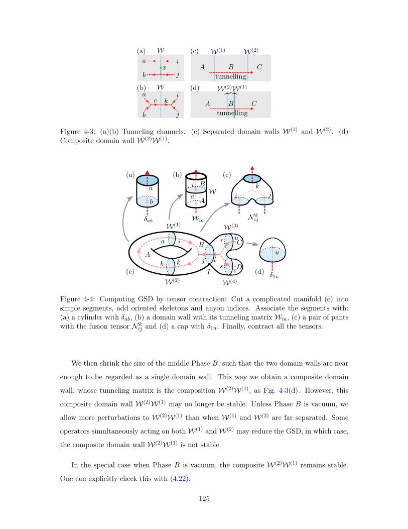
Figure 4-3: (a)(b) Tunneling channels. (c) Separated domain walls 𝒲(1) and 𝒲(2). (d)Composite domain wall 𝒲(2)𝒲(1).
Figure 4-4: Computing GSD by tensor contraction: Cut a complicated manifold (e) intosimple segments, add oriented skeletons and anyon indices. Associate the segments with:(a) a cylinder with 𝛿𝑎𝑏, (b) a domain wall with its tunneling matrix 𝒲𝑖𝑎, (c) a pair of pantswith the fusion tensor 𝒩 𝑘
𝑖𝑗 and (d) a cap with 𝛿1𝑢. Finally, contract all the tensors.
We then shrink the size of the middle Phase 𝐵, such that the two domain walls are near
enough to be regarded as a single domain wall. This way we obtain a composite domain
wall, whose tunneling matrix is the composition 𝒲(2)𝒲(1), as Fig. 4-3(d). However, this
composite domain wall 𝒲(2)𝒲(1) may no longer be stable. Unless Phase 𝐵 is vacuum, we
allow more perturbations to 𝒲(2)𝒲(1) than when 𝒲(1) and 𝒲(2) are far separated. Some
operators simultaneously acting on both𝒲(1) and𝒲(2) may reduce the GSD, in which case,
the composite domain wall 𝒲(2)𝒲(1) is not stable.
In the special case when Phase 𝐵 is vacuum, the composite 𝒲(2)𝒲(1) remains stable.
One can explicitly check this with (4.22).
125
4.1.2.4 GSD in the presence of gapped domain walls
Below we derive the GSD, for a 2D system containing several topological orders separated by
loop-like gapped domain walls. Domain walls cut a whole 2D system into several segments.
Without losing generality, let us consider an example in Fig. 4-4 with topological orders,
Phases 𝐴,𝐵,𝐶,𝐷, and four nontrivial domain walls, 𝒲(1),𝒲(2),𝒲(3),𝒲(4), on a manifold
Fig. 4-4(e). We first add extra trivial domain walls 𝒲 = 𝐼, so that all segments between
domain walls are reduced to simpler topologies: caps, cylinders or pants. We also add
oriented skeletons to the manifold, and put anyon indices on both sides of the domain walls,
shown in Fig. 4-4(e). Next, see Fig. 4-4(a)(b)(c)(d), for the segments with oriented skeletons
and anyon indices, we associate certain tensors: caps with 𝛿1𝑢, cylinders with 𝛿𝑎𝑏, pants with
𝒩 𝑘𝑖𝑗 in the corresponding topological order, and domain walls with their tunneling matrices
𝒲𝑖𝑎. We may reverse the orientation and at the same time replace the index 𝑎 with 𝑎*.
Finally we multiply these tensors together and contract all the anyon indices. Physically
such tensor contraction computes the total number of winding channels of anyons, which
exactly counts the number of ground states, thus the GSD.
Systems with gapped boundaries are included in our method; just imagine that there
are vacuum on caps connected to the boundaries, e.g., Phases 𝐶,𝐷 in Fig. 4-4(e) can be
vacuum. Dimensions of generic fusion spaces can also be calculated, by putting the anyon
𝑎 on the cap and associating the tensor 𝛿𝑎𝑢 instead of 𝛿1𝑢.
We derive GSD on exemplary manifolds:
1. A stable domain wall 𝒲 on the sphere: GSD =𝒲11 = 1.
2. A domain wall 𝒲 on the torus: GSD = Tr(𝒲). Several domain walls 𝒲(1), . . . ,𝒲(𝑛)
on the torus, in Fig. 4-5(a): GSD = Tr(𝒲(1) · · ·𝒲(𝑛)). In particular, Tr[𝒲(1)(𝒲(2))†]
counts the types of 0D defects between 1D gapped domain walls 𝒲(1),𝒲(2).
3. A sphere with punctures: A cylinder with two gapped boundaries 𝒲𝐿 and 𝒲𝑅, in
Fig. 4-5(b): GSD =∑
𝑎𝒲𝐿𝑎1𝒲𝑅
1𝑎. A pair of pants with three gapped boundaries𝒲(1),
𝒲(2) and 𝒲(3), in Fig. 4-5(c): GSD =∑
𝑖𝑗𝑘𝒲(1)𝑖1 𝒲
(2)𝑗1 𝒩 𝑘
𝑖𝑗𝒲(3)1𝑘 .
4. The rocket graph in Fig. 4-4(e): GSD =∑
𝑎,𝑖,𝑗,𝑘,𝑟,𝑠
𝒲(1)𝑖𝑎 𝒲
(2)𝑎𝑘 (𝒩
𝐵)𝑘𝑖𝑗(𝒩𝐵)𝑗𝑟𝑠𝒲(3)𝑟1 𝒲
(4)𝑠1 .
126
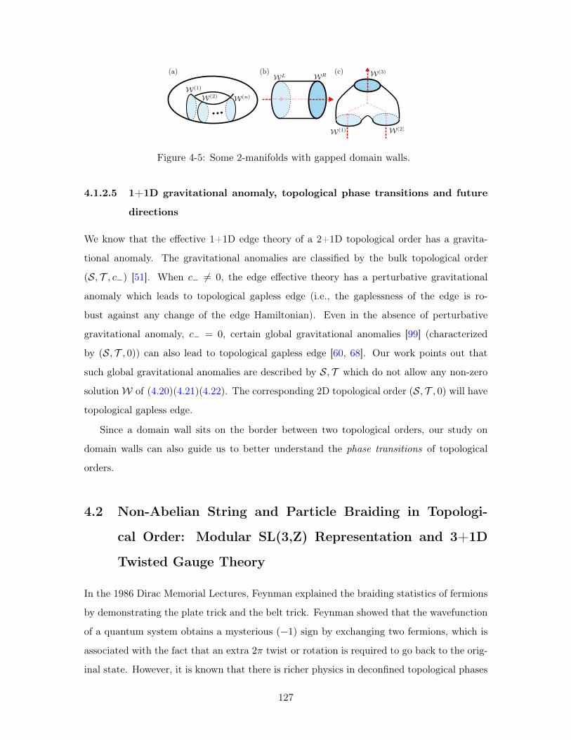
Figure 4-5: Some 2-manifolds with gapped domain walls.
4.1.2.5 1+1D gravitational anomaly, topological phase transitions and future
directions
We know that the effective 1+1D edge theory of a 2+1D topological order has a gravita-
tional anomaly. The gravitational anomalies are classified by the bulk topological order
(𝒮, 𝒯 , 𝑐−) [51]. When 𝑐− = 0, the edge effective theory has a perturbative gravitational
anomaly which leads to topological gapless edge (i.e., the gaplessness of the edge is ro-
bust against any change of the edge Hamiltonian). Even in the absence of perturbative
gravitational anomaly, 𝑐− = 0, certain global gravitational anomalies [99] (characterized
by (𝒮, 𝒯 , 0)) can also lead to topological gapless edge [60, 68]. Our work points out that
such global gravitational anomalies are described by 𝒮, 𝒯 which do not allow any non-zero
solution𝒲 of (4.20)(4.21)(4.22). The corresponding 2D topological order (𝒮, 𝒯 , 0) will have
topological gapless edge.
Since a domain wall sits on the border between two topological orders, our study on
domain walls can also guide us to better understand the phase transitions of topological
orders.
4.2 Non-Abelian String and Particle Braiding in Topologi-
cal Order: Modular SL(3,Z) Representation and 3+1D
Twisted Gauge Theory
In the 1986 Dirac Memorial Lectures, Feynman explained the braiding statistics of fermions
by demonstrating the plate trick and the belt trick. Feynman showed that the wavefunction
of a quantum system obtains a mysterious (−1) sign by exchanging two fermions, which is
associated with the fact that an extra 2𝜋 twist or rotation is required to go back to the orig-
inal state. However, it is known that there is richer physics in deconfined topological phases
127
of 2+1D and 3+1D spacetime. (Here 𝑑+1D is 𝑑-dimensional space and 1-dimensional time,
while 𝑑D is 𝑑-dimensional space.) In 2+1D, there are “anyons” with exotic braiding statistics
for point particles [5]. In 3+1D, Feynman only had to consider bosonic or fermionic statis-
tics for point particles, without worrying about anyonic statistics. Nonetheless, there are
string-like excitations, whose braiding process in 3+1D can enrich the statistics of deconfined
topological phases. In this work, we aim to systematically address the string and particle
braiding statistics in deconfined gapped phases of 3+1D topological orders. Namely, we aim
to determine what statistical phase the wavefunction of the whole system gains under the
string and particle braiding process.
Since the discovery of 2+1D topological orders, we have now gained quite systematic ways
to classify and characterize them, by using the induced representations of the mapping class
group of the T2 torus (the modular group SL(2,Z) and the gauge/Berry phase structure
of ground states and the topology-dependent ground state degeneracy, using the unitary
fusion categories, and using simple current algebra, a pattern of zeros, and field theories.
Our better understanding of topologically ordered states also holds the promises of applying
their rich quantum phenomena, including fractional statistics and non-Abelian anyons, to
topological quantum computation.
However, our understanding of 3+1D topological orders is in its infancy and far from
systematic. This motivates our work attempting to address:
Q1: “How do we (at least partially) classify and characterize 3D topological orders?”
By classification, we mean counting the number of distinct phases of topological orders and
giving them a proper label. By characterization, we mean to describe their properties in
terms of physical observables. Here our approach to studying 𝑑D topological orders is to
simply generalize the above 2D approach, to use the ground state degeneracy (GSD) on
𝑑-torus T𝑑 = (𝑆1)𝑑, and the associated representations of the mapping class group (MCG)
of T𝑑 (recently proposed in Refs.[51]),
MCG(T𝑑) = SL(𝑑,Z). (4.25)
For 3D, the mapping class group SL(3,Z) is generated by the modular transformation S𝑥𝑦𝑧
128
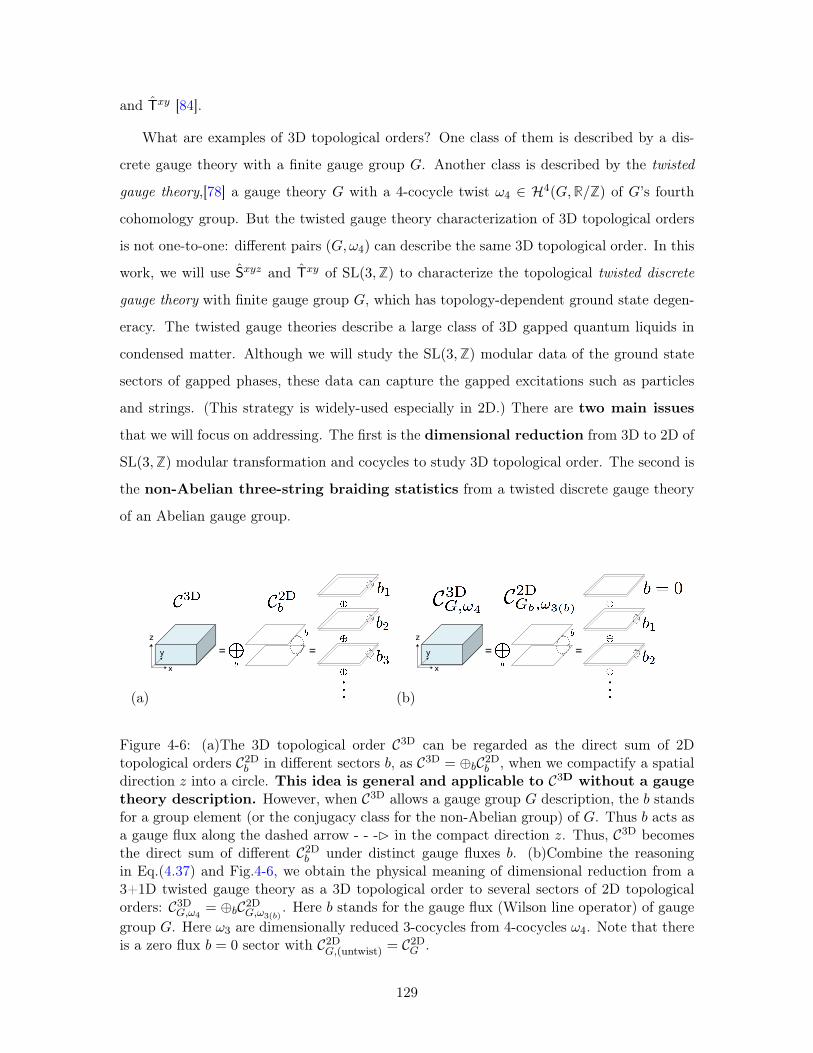
and T𝑥𝑦 [84].
What are examples of 3D topological orders? One class of them is described by a dis-
crete gauge theory with a finite gauge group 𝐺. Another class is described by the twisted
gauge theory,[78] a gauge theory 𝐺 with a 4-cocycle twist 𝜔4 ∈ ℋ4(𝐺,R/Z) of 𝐺’s fourth
cohomology group. But the twisted gauge theory characterization of 3D topological orders
is not one-to-one: different pairs (𝐺,𝜔4) can describe the same 3D topological order. In this
work, we will use S𝑥𝑦𝑧 and T𝑥𝑦 of SL(3,Z) to characterize the topological twisted discrete
gauge theory with finite gauge group 𝐺, which has topology-dependent ground state degen-
eracy. The twisted gauge theories describe a large class of 3D gapped quantum liquids in
condensed matter. Although we will study the SL(3,Z) modular data of the ground state
sectors of gapped phases, these data can capture the gapped excitations such as particles
and strings. (This strategy is widely-used especially in 2D.) There are two main issues
that we will focus on addressing. The first is the dimensional reduction from 3D to 2D of
SL(3,Z) modular transformation and cocycles to study 3D topological order. The second is
the non-Abelian three-string braiding statistics from a twisted discrete gauge theory
of an Abelian gauge group.
(a)
!
"
#
= =
(b)
!
"
#
= =
Figure 4-6: (a)The 3D topological order 𝒞3D can be regarded as the direct sum of 2Dtopological orders 𝒞2D𝑏 in different sectors 𝑏, as 𝒞3D = ⊕𝑏𝒞2D𝑏 , when we compactify a spatialdirection 𝑧 into a circle. This idea is general and applicable to 𝒞3D without a gaugetheory description. However, when 𝒞3D allows a gauge group 𝐺 description, the 𝑏 standsfor a group element (or the conjugacy class for the non-Abelian group) of 𝐺. Thus 𝑏 acts asa gauge flux along the dashed arrow - - -B in the compact direction 𝑧. Thus, 𝒞3D becomesthe direct sum of different 𝒞2D𝑏 under distinct gauge fluxes 𝑏. (b)Combine the reasoningin Eq.(4.37) and Fig.4-6, we obtain the physical meaning of dimensional reduction from a3+1D twisted gauge theory as a 3D topological order to several sectors of 2D topologicalorders: 𝒞3D𝐺,𝜔4
= ⊕𝑏𝒞2D𝐺,𝜔3(𝑏). Here 𝑏 stands for the gauge flux (Wilson line operator) of gauge
group 𝐺. Here 𝜔3 are dimensionally reduced 3-cocycles from 4-cocycles 𝜔4. Note that thereis a zero flux 𝑏 = 0 sector with 𝒞2D𝐺,(untwist) = 𝒞
2D𝐺 .
129
(⋆1) Dimensional Reduction from 3D to 2D: for SL(3,Z) modular S, T matrices
and cocycles - For the first issue, our general philosophy is as follows:
“Since 3D topological orders are foreign and unfamiliar to us, we will dimensionally reduce
3D topological orders to several sectors of 2D topological orders in the Hilbert space of ground
states (not in the real space, see Fig.4-6). Then we will be able to borrow the more familiar
2D topological orders to understand 3D topological orders.”
We will compute the matrices S𝑥𝑦𝑧 and T𝑥𝑦 that generate the SL(3,Z) representation in the
quasi-(particle or string)-excitations basis of 3+1D topological order. We find an explicit
expression of S𝑥𝑦𝑧 and T𝑥𝑦, in terms of the gauge group 𝐺 and the 4-cocycle 𝜔4, for both
Abelian and non-Abelian gauge groups. We note that SL(3,Z) contains a subgroup SL(2,Z),
which is generated by S𝑥𝑦 and T𝑥𝑦.
In the most generic cases of topological orders (potentially without a gauge group de-
scription), the matrices S𝑥𝑦 and T𝑥𝑦 can still be block diagonalized as the sum of several
sectors in the quasi-excitations basis, each sector carrying an index of 𝑏,
S𝑥𝑦 = ⊕𝑏S𝑥𝑦𝑏 , T𝑥𝑦 = ⊕𝑏T𝑥𝑦𝑏 , (4.26)
The pair (S𝑥𝑦𝑏 ,T𝑥𝑦𝑏 ), generating an SL(2,Z) representation, describes a 2D topological order
𝒞2D𝑏 . This leads to a dimension reduction of the 3D topological order 𝒞3D:
𝒞3D = ⊕𝑏𝒞2D𝑏 . (4.27)
In the more specific case, when the topological order allows a gauge group 𝐺 description
which we focus on here, we find that the 𝑏 stands for a gauge flux for group 𝐺 (that is, 𝑏 is
a group element for an Abelian 𝐺, while 𝑏 is a conjugacy class for a non-Abelian 𝐺).
The physical picture of the above dimensional reduction is the following (see Fig.4-6): If
we compactify one of the 3D spatial directions (say the 𝑧 direction) into a small circle, the
3D topological order 𝒞3D can be viewed as a direct sum of 2D topological orders 𝒞2D𝑏 with
(accidental) degenerate ground states at the lowest energy.
130
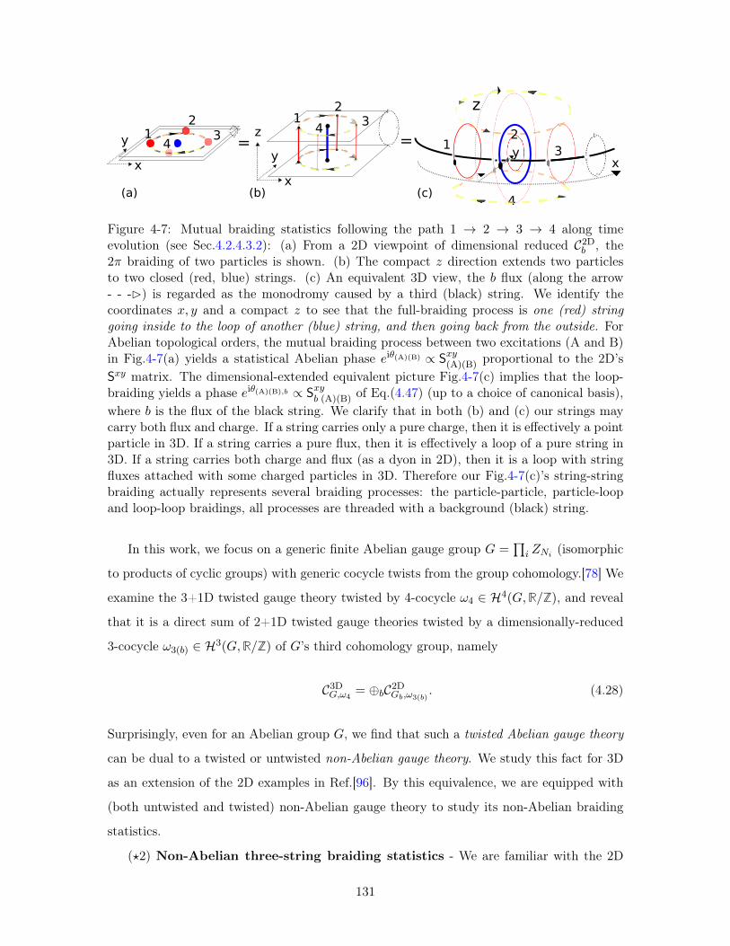
1 34
x
y
z
yx
z
1 3
4
2=
x
y
(a)
=
(b) (c)
12
34
2
Figure 4-7: Mutual braiding statistics following the path 1 → 2 → 3 → 4 along timeevolution (see Sec.4.2.4.3.2): (a) From a 2D viewpoint of dimensional reduced 𝒞2D𝑏 , the2𝜋 braiding of two particles is shown. (b) The compact 𝑧 direction extends two particlesto two closed (red, blue) strings. (c) An equivalent 3D view, the 𝑏 flux (along the arrow- - -B) is regarded as the monodromy caused by a third (black) string. We identify thecoordinates 𝑥, 𝑦 and a compact 𝑧 to see that the full-braiding process is one (red) stringgoing inside to the loop of another (blue) string, and then going back from the outside. ForAbelian topological orders, the mutual braiding process between two excitations (A and B)in Fig.4-7(a) yields a statistical Abelian phase 𝑒i𝜃(A)(B) ∝ S𝑥𝑦(A)(B) proportional to the 2D’sS𝑥𝑦 matrix. The dimensional-extended equivalent picture Fig.4-7(c) implies that the loop-braiding yields a phase 𝑒i𝜃(A)(B),𝑏 ∝ S𝑥𝑦𝑏 (A)(B) of Eq.(4.47) (up to a choice of canonical basis),where 𝑏 is the flux of the black string. We clarify that in both (b) and (c) our strings maycarry both flux and charge. If a string carries only a pure charge, then it is effectively a pointparticle in 3D. If a string carries a pure flux, then it is effectively a loop of a pure string in3D. If a string carries both charge and flux (as a dyon in 2D), then it is a loop with stringfluxes attached with some charged particles in 3D. Therefore our Fig.4-7(c)’s string-stringbraiding actually represents several braiding processes: the particle-particle, particle-loopand loop-loop braidings, all processes are threaded with a background (black) string.
In this work, we focus on a generic finite Abelian gauge group 𝐺 =∏𝑖 𝑍𝑁𝑖 (isomorphic
to products of cyclic groups) with generic cocycle twists from the group cohomology.[78] We
examine the 3+1D twisted gauge theory twisted by 4-cocycle 𝜔4 ∈ ℋ4(𝐺,R/Z), and reveal
that it is a direct sum of 2+1D twisted gauge theories twisted by a dimensionally-reduced
3-cocycle 𝜔3(𝑏) ∈ ℋ3(𝐺,R/Z) of 𝐺’s third cohomology group, namely
𝒞3D𝐺,𝜔4= ⊕𝑏𝒞2D𝐺𝑏,𝜔3(𝑏)
. (4.28)
Surprisingly, even for an Abelian group 𝐺, we find that such a twisted Abelian gauge theory
can be dual to a twisted or untwisted non-Abelian gauge theory. We study this fact for 3D
as an extension of the 2D examples in Ref.[96]. By this equivalence, we are equipped with
(both untwisted and twisted) non-Abelian gauge theory to study its non-Abelian braiding
statistics.
(⋆2) Non-Abelian three-string braiding statistics - We are familiar with the 2D
131
braiding statistics: there is only particle-particle braiding, which yields bosonic, fermionic
or anyonic statistics by braiding a particle around another particle. We find that the 3D
topological order introduces both particle-like and string-like excitations. We aim to address
the question:
Q2: “How do we characterize the braiding statistics of strings and particles in 3+1D topo-
logical orders?”
The possible braiding statistics in 3D learned in the past literature are as follows:
(i) Particle-particle braiding, which can only be bosonic or fermionic due to the absence of
nontrivial braid group in 3D for point particles.
(ii) Particle-string braiding, which is the Aharonov-Bohm effect of Z𝑁 gauge theory, where a
particle such as a Z𝑁 charge braiding around a string (or a vortex line) as Z𝑁 flux, obtaining
a 𝑒i2𝜋𝑁 phase of statistics.
(iii) String-string braiding, where a closed string (a red loop), shown in Fig.4-7(c) excluding
the background black string, wraps around a blue loop. The related idea known as loop-loop
braiding forming the loop braid group has been proposed mathematically.
However, we will address some extra new braiding statistics among three closed strings:
(iv) Three-string braiding, shown in Fig.4-7(c), where a closed string (a red loop) wraps
around another closed string (a blue loop) but the two loops are both threaded by a third
loop (the black string). This braiding configuration is discovered recently by Ref.[76], also
a related work in Ref.[77] for a twisted Abelian gauge theory.
The new ingredient of our work on braiding statistics can be summarized as follows: We
consider the string and particle braiding of general twisted gauge theories with the most
generic finite Abelian gauge group 𝐺 =∏𝑢 𝑍𝑁𝑢 , labeled by the data (𝐺,𝜔4). We provide
a 3D to 2D dimensional reduction approach to realize the three-string braiding statistics
of Fig.4-7. We first show that the SL(2,Z) representations (S𝑥𝑦𝑏 ,T𝑥𝑦𝑏 ) fully encode this
particular type of Abelian three-closed-string statistics shown in Fig.4-7. We further find
that, for a twisted gauge theory with an Abelian (𝑍𝑁 )4 group, certain 4-cocycles (called
as Type IV 4-cocycles) will make the twisted theory to be a non-Abelian theory. More
precisely, while the two-string braiding statistics of unlink is Abelian, the three-
string braiding statistics of Hopf links, obtained from threading the two strings
132
with the third string, will become non-Abelian. We also demonstrate that (S𝑥𝑦𝑏
encodes this three-string braiding statistics.
4.2.1 Twisted Gauge Theory and Cocycles of Group Cohomology
In this section, we aim to address the question:
Q3: “How to formulate or construct certain 3+1D topological orders on the lattice?”
We will consider 3+1D twisted discrete gauge theories. Our motivation to study the
discrete gauge theory is that it is topological and exhibits Aharonov-Bohm phenomena.
One approach to formulating a discrete gauge theory is the lattice gauge theory.[100] A
famous example in both high energy and condensed matter communities is the 𝑍2 discrete
gauge theory in 2+1D (also called the 𝑍2 toric code, 𝑍2 spin liquids, 𝑍2 topological order).
Kitaev’s toric code and quantum double model[69] provides a simple Hamiltonian,
𝐻 = −∑𝑣
𝐴𝑣 −∑𝑝
𝐵𝑝, (4.29)
where a space lattice formalism is used, and 𝐴𝑣 is the vertex operator acting on the vertex
𝑣, 𝐵𝑝 is the plaquette (or face) term to ensure the zero flux condition on each plaquette.
Both 𝐴𝑣 and 𝐵𝑝 consist of only Pauli spin operators for the 𝑍2 model. Such ground states of
the Hamiltonian are found to be 𝑍2 gauge theory with |𝐺|2 = 4-fold topological degeneracy
on the T2 torus. Its generalization to a twisted 𝑍2 gauge theory is the 𝑍2 double-semions
model, captured by the framework of the Levin-Wen string-net model [101, 11].
4.2.2 Canonical basis and the generalized twisted quantum double model
𝐷𝜔(𝐺) to 3D triple basis
In Chap.??, we have formulated a Dijkgraaf-Witten topological gauge theory as higher di-
mensional TOs. Thus we have answered the question Q3 using the spacetime-lattice path
integral. Our next goal is to construct its Hamiltonian on the space lattice, and to find a
good basis representing its quasi-excitations, such that we can efficiently read the informa-
tion of O(S𝑥𝑦𝑧,T𝑥𝑦) in this canonical basis. We will outline the twisted quantum double model
generalized to 3D as the exactly soluble model in the next subsection, where the canonical
basis can diagonalize its Hamiltonian.
133
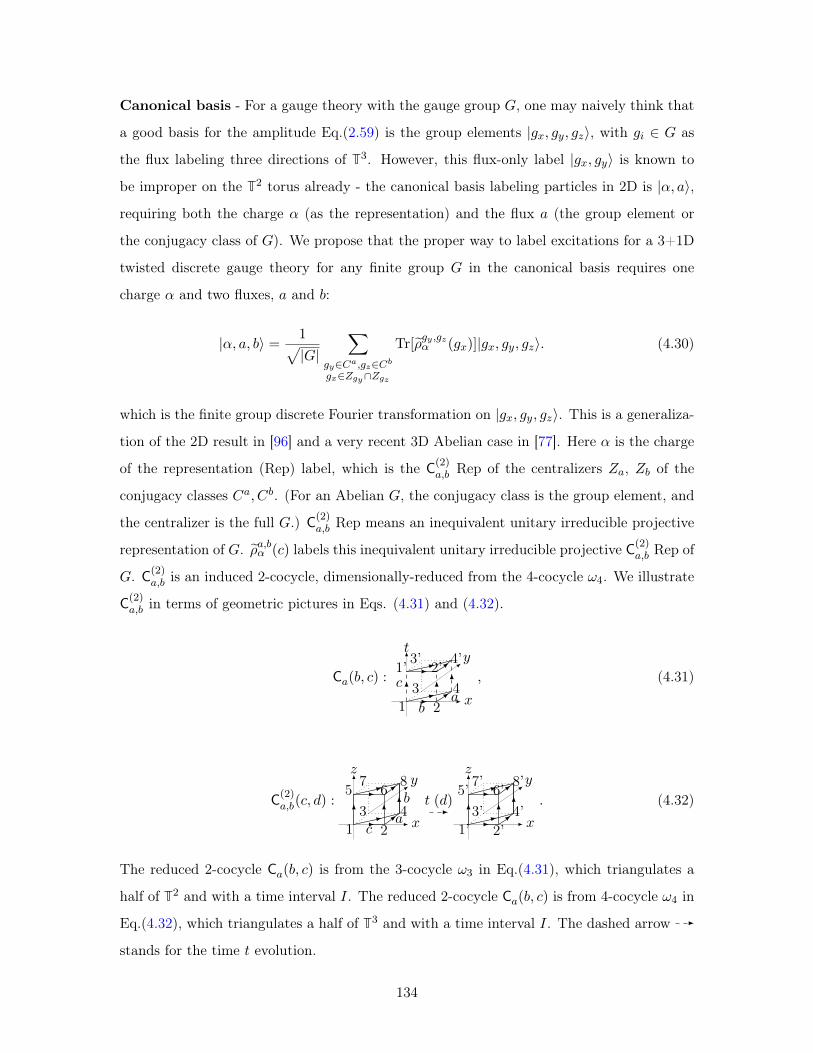
Canonical basis - For a gauge theory with the gauge group 𝐺, one may naively think that
a good basis for the amplitude Eq.(2.59) is the group elements |𝑔𝑥, 𝑔𝑦, 𝑔𝑧⟩, with 𝑔𝑖 ∈ 𝐺 as
the flux labeling three directions of T3. However, this flux-only label |𝑔𝑥, 𝑔𝑦⟩ is known to
be improper on the T2 torus already - the canonical basis labeling particles in 2D is |𝛼, 𝑎⟩,
requiring both the charge 𝛼 (as the representation) and the flux 𝑎 (the group element or
the conjugacy class of 𝐺). We propose that the proper way to label excitations for a 3+1D
twisted discrete gauge theory for any finite group 𝐺 in the canonical basis requires one
charge 𝛼 and two fluxes, 𝑎 and 𝑏:
|𝛼, 𝑎, 𝑏⟩ = 1√|𝐺|
∑𝑔𝑦∈𝐶𝑎,𝑔𝑧∈𝐶𝑏
𝑔𝑥∈𝑍𝑔𝑦∩𝑍𝑔𝑧
Tr[𝜌𝑔𝑦 ,𝑔𝑧𝛼 (𝑔𝑥)]|𝑔𝑥, 𝑔𝑦, 𝑔𝑧⟩. (4.30)
which is the finite group discrete Fourier transformation on |𝑔𝑥, 𝑔𝑦, 𝑔𝑧⟩. This is a generaliza-
tion of the 2D result in [96] and a very recent 3D Abelian case in [77]. Here 𝛼 is the charge
of the representation (Rep) label, which is the C(2)𝑎,𝑏 Rep of the centralizers 𝑍𝑎, 𝑍𝑏 of the
conjugacy classes 𝐶𝑎, 𝐶𝑏. (For an Abelian 𝐺, the conjugacy class is the group element, and
the centralizer is the full 𝐺.) C(2)𝑎,𝑏 Rep means an inequivalent unitary irreducible projective
representation of 𝐺. 𝜌𝑎,𝑏𝛼 (𝑐) labels this inequivalent unitary irreducible projective C(2)𝑎,𝑏 Rep of
𝐺. C(2)𝑎,𝑏 is an induced 2-cocycle, dimensionally-reduced from the 4-cocycle 𝜔4. We illustrate
C(2)𝑎,𝑏 in terms of geometric pictures in Eqs. (4.31) and (4.32).
C𝑎(𝑏, 𝑐) :
1
1’
23 4
2’3’ 4’
𝑥
𝑦𝑡
𝑐𝑎
𝑏
, (4.31)
C(2)𝑎,𝑏(𝑐, 𝑑) :
1
5
23 4
67 8
𝑥
𝑦𝑧
𝑏
𝑎𝑐
𝑡 (𝑑)
1’
5’
2’3’ 4’
6’7’ 8’
𝑥
𝑦𝑧
. (4.32)
The reduced 2-cocycle C𝑎(𝑏, 𝑐) is from the 3-cocycle 𝜔3 in Eq.(4.31), which triangulates a
half of T2 and with a time interval 𝐼. The reduced 2-cocycle C𝑎(𝑏, 𝑐) is from 4-cocycle 𝜔4 in
Eq.(4.32), which triangulates a half of T3 and with a time interval 𝐼. The dashed arrow
stands for the time 𝑡 evolution.
134
The 𝜌𝑔𝑦 ,𝑔𝑧𝛼 (𝑔𝑥) values are determined by the C(2)𝑎,𝑏 projective representation formula:
𝜌𝑎,𝑏𝛼 (𝑐)𝜌𝑎,𝑏𝛼 (𝑑) = C(2)𝑎,𝑏(𝑐, 𝑑)𝜌𝑎,𝑏𝛼 (𝑐𝑑). (4.33)
The trace term Tr[𝜌𝑔𝑦 ,𝑔𝑧𝛼 (𝑔𝑥)] is called the character in the math literature. One can view
the charge 𝛼𝑥 along 𝑥 direction, the flux 𝑎, 𝑏 along the 𝑦, 𝑧.
We first recall that, in 2D, a reduced 2-cocycle C𝑎(𝑏, 𝑐) comes from a slant product
𝑖𝑎𝜔(𝑏, 𝑐) of 3-cocycles, [96] [96] which is geometrically equivalent to filling three 3-cocycles
in a triangular prism of Eq.(4.31). This is known to present the projective representation𝜌𝑎𝛼(𝑏)𝜌𝑎𝛼(𝑐) = C𝑎(𝑏, 𝑐)𝜌𝑎𝛼(𝑏𝑐), because the induced 2-cocycle belongs to the second cohomology
group ℋ2(𝐺,R/Z).[102] (See its explicit triangulation and a novel use of the projective
representation in Sec VI.B. of Ref.[56].)
Similarly, in 3D, a reduced 2-cocycle C𝑎(𝑏, 𝑐) comes from doing twice of the slant products
of 4-cocycles forming the geometry of Eq.(4.32), and renders
C(2)𝑎,𝑏 = 𝑖𝑏(C𝑎(𝑐, 𝑑)) = 𝑖𝑏(𝑖𝑎𝜔(𝑐, 𝑑)), (4.34)
presenting the C(2)𝑎,𝑏-projective representation in Eq.(4.33), where 𝜌𝑎,𝑏𝛼 (𝑐): (𝑍𝑎, 𝑍𝑏)→GL (𝑍𝑎, 𝑍𝑏)
can be written as a matrix in the general linear (GL) group. This 3D generalization for the
canonical basis in Eq.(4.30) is not only natural, but also consistent to 2D when we turn off
the flux along 𝑧 direction (e.g. set 𝑏 = 0). which reduces 3D’s |𝛼, 𝑎, 𝑏⟩ to |𝛼, 𝑎⟩ in the 2D case.
Generalizing 2D twisted quantum double model 𝐷𝜔(𝐺) to 3D: twisted quantum
triple model? – A natural way to combine the Dijkgraaf-Witten theory with Kitaev’s quan-
tum double model Hamiltonian approach will enable us to study the Hamiltonian formalism
for the twisted gauge theory, which is achieved in Ref.[103],[102] for 2+1D, named as the
twisted quantum double model. In 2D, the widely-used notation 𝐷𝜔(𝐺) implies the twisted
quantum double model with its gauge group 𝐺 and its cocycle twist 𝜔. It is straightforward
to generalize their results to 3+1D.
To construct the Hamiltonian on the 3D spatial lattice, we follow [103] with the form
of the twisted quantum double model Hamiltonian of Eq.(4.29) and put the system on
the T3 torus. However, some modification for 3D are adopted: the vertex operator 𝐴𝑣 =
|𝐺|−1∑
[𝑣𝑣′]=𝑔∈𝐺𝐴𝑔𝑣 acts on the vertices of the lattice by lifting the vertex point 𝑣 to 𝑣′
135
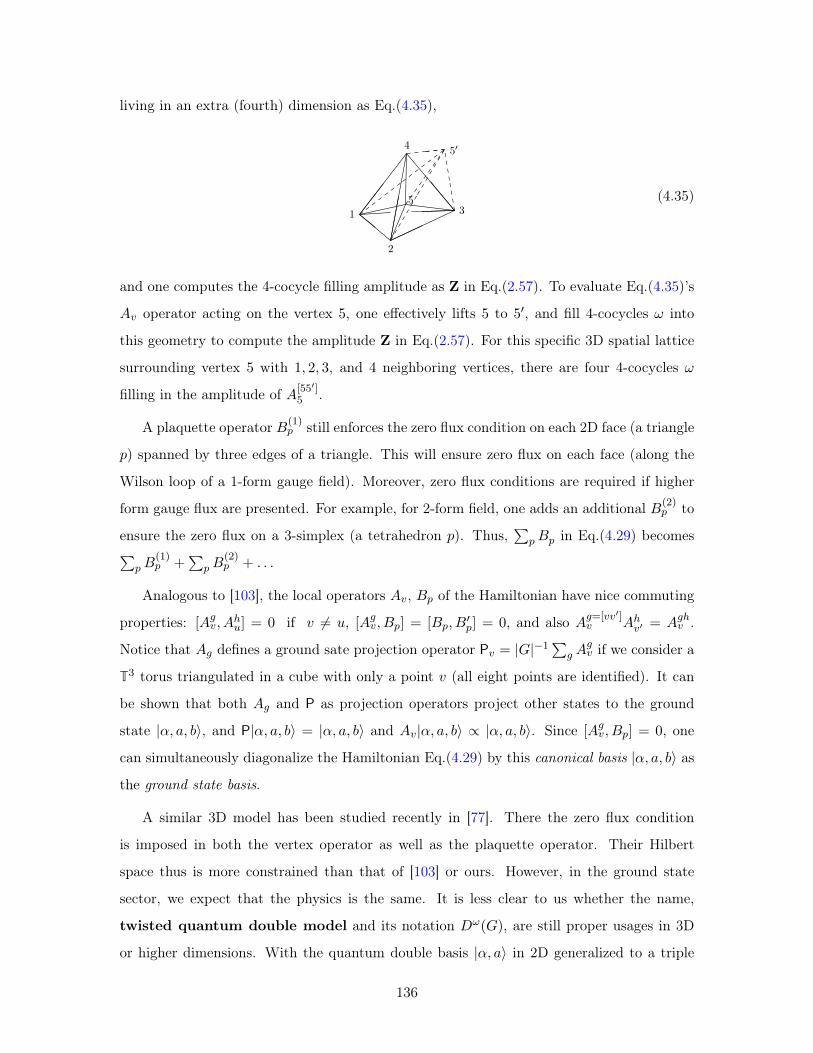
living in an extra (fourth) dimension as Eq.(4.35),
1
2
3
45′
5 (4.35)
and one computes the 4-cocycle filling amplitude as Z in Eq.(2.57). To evaluate Eq.(4.35)’s
𝐴𝑣 operator acting on the vertex 5, one effectively lifts 5 to 5′, and fill 4-cocycles 𝜔 into
this geometry to compute the amplitude Z in Eq.(2.57). For this specific 3D spatial lattice
surrounding vertex 5 with 1, 2, 3, and 4 neighboring vertices, there are four 4-cocycles 𝜔
filling in the amplitude of 𝐴[55′]5 .
A plaquette operator 𝐵(1)𝑝 still enforces the zero flux condition on each 2D face (a triangle
𝑝) spanned by three edges of a triangle. This will ensure zero flux on each face (along the
Wilson loop of a 1-form gauge field). Moreover, zero flux conditions are required if higher
form gauge flux are presented. For example, for 2-form field, one adds an additional 𝐵(2)𝑝 to
ensure the zero flux on a 3-simplex (a tetrahedron 𝑝). Thus,∑
𝑝𝐵𝑝 in Eq.(4.29) becomes∑𝑝𝐵
(1)𝑝 +
∑𝑝𝐵
(2)𝑝 + . . .
Analogous to [103], the local operators 𝐴𝑣, 𝐵𝑝 of the Hamiltonian have nice commuting
properties: [𝐴𝑔𝑣, 𝐴ℎ𝑢] = 0 if 𝑣 = 𝑢, [𝐴𝑔𝑣, 𝐵𝑝] = [𝐵𝑝, 𝐵′𝑝] = 0, and also 𝐴
𝑔=[𝑣𝑣′]𝑣 𝐴ℎ𝑣′ = 𝐴𝑔ℎ𝑣 .
Notice that 𝐴𝑔 defines a ground sate projection operator P𝑣 = |𝐺|−1∑
𝑔 𝐴𝑔𝑣 if we consider a
T3 torus triangulated in a cube with only a point 𝑣 (all eight points are identified). It can
be shown that both 𝐴𝑔 and P as projection operators project other states to the ground
state |𝛼, 𝑎, 𝑏⟩, and P|𝛼, 𝑎, 𝑏⟩ = |𝛼, 𝑎, 𝑏⟩ and 𝐴𝑣|𝛼, 𝑎, 𝑏⟩ ∝ |𝛼, 𝑎, 𝑏⟩. Since [𝐴𝑔𝑣, 𝐵𝑝] = 0, one
can simultaneously diagonalize the Hamiltonian Eq.(4.29) by this canonical basis |𝛼, 𝑎, 𝑏⟩ as
the ground state basis.
A similar 3D model has been studied recently in [77]. There the zero flux condition
is imposed in both the vertex operator as well as the plaquette operator. Their Hilbert
space thus is more constrained than that of [103] or ours. However, in the ground state
sector, we expect that the physics is the same. It is less clear to us whether the name,
twisted quantum double model and its notation 𝐷𝜔(𝐺), are still proper usages in 3D
or higher dimensions. With the quantum double basis |𝛼, 𝑎⟩ in 2D generalized to a triple
136
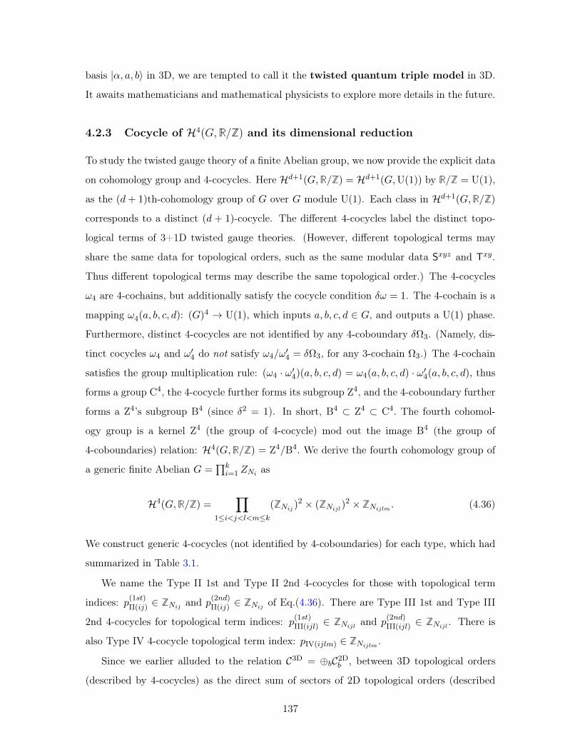
basis |𝛼, 𝑎, 𝑏⟩ in 3D, we are tempted to call it the twisted quantum triple model in 3D.
It awaits mathematicians and mathematical physicists to explore more details in the future.
4.2.3 Cocycle of ℋ4(𝐺,R/Z) and its dimensional reduction
To study the twisted gauge theory of a finite Abelian group, we now provide the explicit data
on cohomology group and 4-cocycles. Here ℋ𝑑+1(𝐺,R/Z) = ℋ𝑑+1(𝐺,U(1)) by R/Z = U(1),
as the (𝑑+ 1)th-cohomology group of 𝐺 over 𝐺 module U(1). Each class in ℋ𝑑+1(𝐺,R/Z)
corresponds to a distinct (𝑑 + 1)-cocycle. The different 4-cocycles label the distinct topo-
logical terms of 3+1D twisted gauge theories. (However, different topological terms may
share the same data for topological orders, such as the same modular data S𝑥𝑦𝑧 and T𝑥𝑦.
Thus different topological terms may describe the same topological order.) The 4-cocycles
𝜔4 are 4-cochains, but additionally satisfy the cocycle condition 𝛿𝜔 = 1. The 4-cochain is a
mapping 𝜔4(𝑎, 𝑏, 𝑐, 𝑑): (𝐺)4 → U(1), which inputs 𝑎, 𝑏, 𝑐, 𝑑 ∈ 𝐺, and outputs a U(1) phase.
Furthermore, distinct 4-cocycles are not identified by any 4-coboundary 𝛿Ω3. (Namely, dis-
tinct cocycles 𝜔4 and 𝜔′4 do not satisfy 𝜔4/𝜔
′4 = 𝛿Ω3, for any 3-cochain Ω3.) The 4-cochain
satisfies the group multiplication rule: (𝜔4 · 𝜔′4)(𝑎, 𝑏, 𝑐, 𝑑) = 𝜔4(𝑎, 𝑏, 𝑐, 𝑑) · 𝜔′
4(𝑎, 𝑏, 𝑐, 𝑑), thus
forms a group C4, the 4-cocycle further forms its subgroup Z4, and the 4-coboundary further
forms a Z4’s subgroup B4 (since 𝛿2 = 1). In short, B4 ⊂ Z4 ⊂ C4. The fourth cohomol-
ogy group is a kernel Z4 (the group of 4-cocycle) mod out the image B4 (the group of
4-coboundaries) relation: ℋ4(𝐺,R/Z) = Z4/B4. We derive the fourth cohomology group of
a generic finite Abelian 𝐺 =∏𝑘𝑖=1 𝑍𝑁𝑖 as
ℋ4(𝐺,R/Z) =∏
1≤𝑖<𝑗<𝑙<𝑚≤𝑘(Z𝑁𝑖𝑗 )
2 × (Z𝑁𝑖𝑗𝑙)2 × Z𝑁𝑖𝑗𝑙𝑚
. (4.36)
We construct generic 4-cocycles (not identified by 4-coboundaries) for each type, which had
summarized in Table 3.1.
We name the Type II 1st and Type II 2nd 4-cocycles for those with topological term
indices: 𝑝(1𝑠𝑡)II(𝑖𝑗) ∈ Z𝑁𝑖𝑗 and 𝑝(2𝑛𝑑)II(𝑖𝑗) ∈ Z𝑁𝑖𝑗 of Eq.(4.36). There are Type III 1st and Type III
2nd 4-cocycles for topological term indices: 𝑝(1𝑠𝑡)III(𝑖𝑗𝑙) ∈ Z𝑁𝑖𝑗𝑙and 𝑝
(2𝑛𝑑)III(𝑖𝑗𝑙) ∈ Z𝑁𝑖𝑗𝑙
. There is
also Type IV 4-cocycle topological term index: 𝑝IV(𝑖𝑗𝑙𝑚) ∈ Z𝑁𝑖𝑗𝑙𝑚.
Since we earlier alluded to the relation 𝒞3D = ⊕𝑏𝒞2D𝑏 , between 3D topological orders
(described by 4-cocycles) as the direct sum of sectors of 2D topological orders (described
137
by 3-cocycles), we wish to see how the dimensionally-reduced 3-cocycle from 4-cocycles
can hint at the 𝒞2D𝑏 theory of 2D. The geometric interpretation of the induced 3-cocycle
C𝑏(𝑎, 𝑐, 𝑑) ≡ 𝑖𝑏𝜔4(𝑎, 𝑐, 𝑑) is derived from the 4-cocycle 𝜔4:
C𝑏(𝑎, 𝑐, 𝑑) :
1 24
8
𝑥
𝑦𝑧
𝑏
𝑎𝑐
𝑡 (𝑑)
1’ 2’4’
8’
𝑥
𝑦𝑧
(4.37)
The combination of Eq.(4.37) (with four 4-cocycles filling) times the contribution of Eq.(4.31)
(with three 3-cocycles filling) will produce Eq.(4.32) with twelve 4-cocycles filling. Luckily,
the Type II and III 𝜔4 have a simpler form of C𝑏(𝑎, 𝑐, 𝑑) = 𝜔4(𝑎, 𝑏, 𝑐, 𝑑)/𝜔4(𝑏, 𝑎, 𝑐, 𝑑), while
the reduced form of Type IV 𝜔4 is more involved.
This indeed promisingly suggests the relation in Eq.(4.28), 𝒞3D𝐺,𝜔4= ⊕𝑏𝒞2D𝐺,𝜔3(𝑏)
with 𝐺𝑏 =
𝐺 the original group. If we view 𝑏 as the gauge flux along the 𝑧 direction, and compactify 𝑧
into a circle, then a single winding around 𝑧 acts as a monodromy defect carrying the gauge
flux 𝑏 (group elements or conjugacy classes).This implies a geometric picture in Fig.4-6.
One can tentatively write down a relation,
𝒞3D𝐺,𝜔4= 𝒞2D𝐺,1(untwist) ⊕𝑏 =0 𝒞2D𝐺,𝜔3(𝑏)
. (4.38)
There is a zero flux 𝑏 = 0 sector 𝒞2D𝐺,1(untwist) (with 𝜔3 = 1) where the 2D gauge theory with
𝐺 is untwisted. There are other direct sums of 𝒞2D𝐺,𝜔3(𝑏)with nonzero 𝑏 flux insertion that
have twisted 𝜔3(𝑏).
However, different cocycles can represent the same topological order with the equivalent
modular data, in the next section, we should examine this Eq.(4.38) more carefully not in
terms of cocycles, but in terms of the modular data S𝑥𝑦𝑧 and T𝑥𝑦.
4.2.4 Representation for S𝑥𝑦𝑧 and T𝑥𝑦
Q4: “What are the generic expressions of SL(3,Z) modular data?”
First, in Sec.2.6, we apply the cocycle approach using the spacetime path integral with
SL(3,Z) transformation acting along the time evolution to formulate the SL(3,Z) modular
data, and then in Sec 4.2.4.2 we use the more powerful Representation (Rep) Theory to
determine the general expressions of those data in terms of (𝐺,𝜔4).
138
4.2.4.1 Path Integral and Cocycle approach
The cocycles approach uses the spacetime lattice formalism, where we triangulate the
spacetime complex of a 4-manifold ℳ = T3 × 𝐼, (a T3 torus times a time interval 𝐼) of
Eq.(2.63),(2.64),(2.65) into 4-simplices. We then apply the path integral Z in Eq.(2.57) and
the amplitude form in Eq.(2.59) to obtain
T𝑥𝑦(A)(B) = ⟨ΨA|T𝑥𝑦|ΨB⟩, (4.39)
S𝑥𝑦(A)(B) = ⟨ΨA|S𝑥𝑦|ΨB⟩, (4.40)
S𝑥𝑦𝑧(A)(B) = ⟨ΨA|S𝑥𝑦𝑧|ΨB⟩, (4.41)
GSD = Tr[P] =∑𝐴
⟨ΨA|P|ΨA⟩. (4.42)
Here |ΨA⟩ and |ΨB⟩ are ground state bases on the T𝑑 torus, for example, they are |𝛼, 𝑎⟩
(with 𝛼 charge and 𝑎 flux) in 2+1D and |𝛼, 𝑎, 𝑏⟩ (with 𝛼 charge and 𝑎, 𝑏 fluxes) in 3+1D.
We also include the data of GSD, where the P is the projection operator to ground states
discussed in Sec.4.2.2. In the case of d-D GSD on T𝑑 (e.g. 3D GSD on T3), we simply
compute the Z amplitude filling in T𝑑×𝑆1 = T𝑑+1. There is no short cut here except doing
explicit calculations.
4.2.4.2 Representation Theory approach
The cocycle approach in Sec.4.2.4.1 provides nice physical intuition about the modular trans-
formation process. However, the calculation is tedious. There is a powerful approach simply
using Representation Theory, we will present the general formula of S𝑥𝑦𝑠, T𝑥𝑦, S𝑥𝑦 data in
terms of (𝐺,𝜔4) directly. The three steps are outlined as follows:
(i) Obtain the Eq.(4.34)’s C(2)𝑎,𝑏 by doing the slant product twice from 4-cocycle 𝜔4, or tri-
angulating Eq.4.31. (ii) Derive 𝜌𝑎,𝑏𝛼 (𝑐) of C(2)𝑎,𝑏-projective representation in Eq.(4.33), which𝜌𝑎,𝑏𝛼 (𝑐) is a general linear matrix.
(iii) Write the modular data in the canonical basis |𝛼, 𝑎, 𝑏⟩, |𝛽, 𝑐, 𝑑⟩ of Eq.(4.30).
After some long computations, we find the most general formula S𝑥𝑦𝑧 for a group 𝐺
139
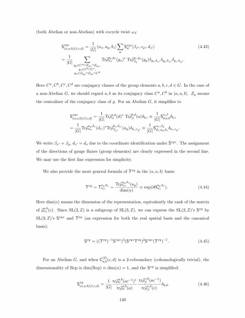
(both Abelian or non-Abelian) with cocycle twist 𝜔4:
S𝑥𝑦𝑧(𝛼,𝑎,𝑏)(𝛽,𝑐,𝑑) =1
|𝐺|⟨𝛼𝑥, 𝑎𝑦, 𝑏𝑧|
∑𝑤
S𝑥𝑦𝑧𝑤 |𝛽𝑥′ , 𝑐𝑦′ , 𝑑𝑧′⟩ (4.43)
=1
|𝐺|∑
𝑔𝑦∈𝐶𝑎∩𝑍𝑔𝑧∩𝑍𝑔𝑥 ,
𝑔𝑧∈𝐶𝑏∩𝐶𝑐,𝑔𝑥∈𝑍𝑔𝑦∩𝑍𝑔𝑧∩𝐶𝑑
Tr𝜌𝑔𝑦 ,𝑔𝑧𝛼𝑥 (𝑔𝑥)* Tr𝜌𝑔𝑧 ,𝑔𝑥𝛽𝑦
(𝑔𝑦)𝛿𝑔𝑥,ℎ𝑧′ 𝛿𝑔𝑦 ,ℎ𝑥′ 𝛿𝑔𝑧 ,ℎ𝑦′ .
Here 𝐶𝑎, 𝐶𝑏, 𝐶𝑐, 𝐶𝑑 are conjugacy classes of the group elements 𝑎, 𝑏, 𝑐, 𝑑 ∈ 𝐺. In the case of
a non-Abelian 𝐺, we should regard 𝑎, 𝑏 as its conjugacy class 𝐶𝑎, 𝐶𝑏 in |𝛼, 𝑎, 𝑏⟩. 𝑍𝑔 means
the centralizer of the conjugacy class of 𝑔. For an Abelian 𝐺, it simplifies to
S𝑥𝑦𝑧(𝛼,𝑎,𝑏)(𝛽,𝑐,𝑑) =1
|𝐺|Tr𝜌𝑎,𝑏𝛼 (𝑑)* Tr𝜌𝑏,𝑑𝛽 (𝑎)𝛿𝑏,𝑐 ≡
1
|𝐺|S𝛼,𝛽𝑑,𝑎,𝑏𝛿𝑏,𝑐
=1
|𝐺|Tr𝜌𝑎𝑦 ,𝑏𝑧𝛼𝑥 (𝑑𝑧′)
*Tr𝜌𝑏𝑧 ,𝑑𝑧′𝛽𝑥′(𝑎𝑦)𝛿𝑏𝑧 ,𝑐𝑦′ ≡
1
|𝐺|S𝛼𝑥,𝛽𝑦𝑑𝑥,𝑎𝑦 ,𝑏𝑧
𝛿𝑏𝑧 ,𝑐𝑦′ .
We write 𝛽𝑥′ = 𝛽𝑦, 𝑑𝑧′ = 𝑑𝑥 due to the coordinate identification under S𝑥𝑦𝑧. The assignment
of the directions of gauge fluxes (group elements) are clearly expressed in the second line.
We may use the first line expression for simplicity.
We also provide the most general formula of T𝑥𝑦 in the |𝛼, 𝑎, 𝑏⟩ basis:
T𝑥𝑦 = T𝑎𝑦 ,𝑏𝑧𝛼𝑥 =
Tr𝜌𝑎𝑦 ,𝑏𝑧𝛼𝑥 (𝑎𝑦)
dim(𝛼)≡ exp(iΘ𝑎𝑦 ,𝑏𝑧
𝛼𝑥 ). (4.44)
Here dim(𝛼) means the dimension of the representation, equivalently the rank of the matrix
of 𝜌𝑎,𝑏𝛼𝑥 (𝑐). Since SL(2,Z) is a subgroup of SL(3,Z), we can express the SL(2,Z)’s S𝑥𝑦 by
SL(3,Z)’s S𝑥𝑦𝑧 and T𝑥𝑦 (an expression for both the real spatial basis and the canonical
basis):
S𝑥𝑦 = ((T𝑥𝑦)−1S𝑥𝑦𝑧)3(S𝑥𝑦𝑧T𝑥𝑦)2S𝑥𝑦𝑧(T𝑥𝑦)−1. (4.45)
For an Abelian 𝐺, and when C(2)𝑎,𝑏(𝑐, 𝑑) is a 2-coboundary (cohomologically trivial), the
dimensionality of Rep is dim(Rep) ≡ dim(𝛼) = 1, and the S𝑥𝑦 is simplified:
S𝑥𝑦(𝛼,𝑎,𝑏)(𝛽,𝑐,𝑑) =1
|𝐺|tr𝜌𝑎,𝑏𝛼 (𝑎𝑐−1)*
tr𝜌𝑎,𝑏𝛼 (𝑎)
tr𝜌𝑐,𝑑𝛽 (𝑎𝑐−1)
tr𝜌𝑐,𝑑𝛽 (𝑐)𝛿𝑏,𝑑. (4.46)
140
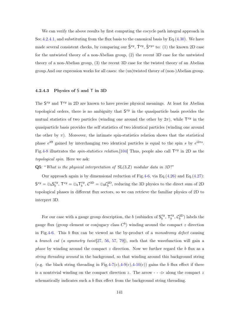
We can verify the above results by first computing the cocycle path integral approach in
Sec.4.2.4.1, and substituting from the flux basis to the canonical basis by Eq.(4.30). We have
made several consistent checks, by comparing our S𝑥𝑦, T𝑥𝑦, S𝑥𝑦𝑧 to: (1) the known 2D case
for the untwisted theory of a non-Abelian group, (2) the recent 3D case for the untwisted
theory of a non-Abelian group, (3) the recent 3D case for the twisted theory of an Abelian
group.And our expression works for all cases: the (un)twisted theory of (non-)Abelian group.
4.2.4.3 Physics of S and T in 3D
The S𝑥𝑦 and T𝑥𝑦 in 2D are known to have precise physical meanings. At least for Abelian
topological orders, there is no ambiguity that S𝑥𝑦 in the quasiparticle basis provides the
mutual statistics of two particles (winding one around the other by 2𝜋), while T𝑥𝑦 in the
quasiparticle basis provides the self statistics of two identical particles (winding one around
the other by 𝜋). Moreover, the intimate spin-statistics relation shows that the statistical
phase 𝑒iΘ gained by interchanging two identical particles is equal to the spin 𝑠 by 𝑒i2𝜋𝑠.
Fig.4-8 illustrates the spin-statistics relation.[104] Thus, people also call T𝑥𝑦 in 2D as the
topological spin. Here we ask:
Q5: “What is the physical interpretation of SL(3,Z) modular data in 3D?”
Our approach again is by dimensional reduction of Fig.4-6, via Eq.(4.26) and Eq.(4.27):
S𝑥𝑦 = ⊕𝑏S𝑥𝑦𝑏 , T𝑥𝑦 = ⊕𝑏T𝑥𝑦𝑏 , 𝒞3D = ⊕𝑏𝒞2D𝑏 , reducing the 3D physics to the direct sum of 2D
topological phases in different flux sectors, so we can retrieve the familiar physics of 2D to
interpret 3D.
For our case with a gauge group description, the 𝑏 (subindex of S𝑥𝑦𝑏 , T𝑥𝑦𝑏 , 𝒞2D𝑏 ) labels the
gauge flux (group element or conjugacy class 𝐶𝑏) winding around the compact 𝑧 direction
in Fig.4-6. This 𝑏 flux can be viewed as the by-product of a monodromy defect causing
a branch cut (a symmetry twist [27, 56, 57, 79]), such that the wavefunction will gain a
phase by winding around the compact 𝑧 direction. Now we further regard the 𝑏 flux as a
string threading around in the background, so that winding around this background string
(e.g. the black string threading in Fig.4-7(c),4-9(c),4-10(c)) gains the 𝑏 flux effect if there
is a nontrivial winding on the compact direction 𝑧. The arrow - - -B along the compact 𝑧
schematically indicates such a 𝑏 flux effect from the background string threading.
141
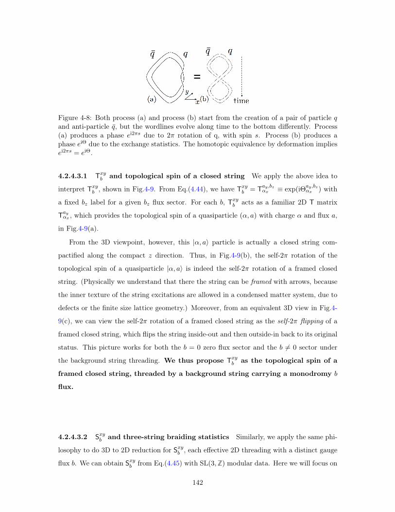
=
Figure 4-8: Both process (a) and process (b) start from the creation of a pair of particle 𝑞and anti-particle 𝑞, but the wordlines evolve along time to the bottom differently. Process(a) produces a phase 𝑒i2𝜋𝑠 due to 2𝜋 rotation of q, with spin 𝑠. Process (b) produces aphase 𝑒iΘ due to the exchange statistics. The homotopic equivalence by deformation implies𝑒i2𝜋𝑠 = 𝑒iΘ.
4.2.4.3.1 T𝑥𝑦𝑏 and topological spin of a closed string We apply the above idea to
interpret T𝑥𝑦𝑏 , shown in Fig.4-9. From Eq.(4.44), we have T𝑥𝑦𝑏 = T𝑎𝑦 ,𝑏𝑧𝛼𝑥 ≡ exp(iΘ𝑎𝑦 ,𝑏𝑧
𝛼𝑥 ) with
a fixed 𝑏𝑧 label for a given 𝑏𝑧 flux sector. For each 𝑏, T𝑥𝑦𝑏 acts as a familiar 2D T matrix
T𝑎𝑦𝛼𝑥 , which provides the topological spin of a quasiparticle (𝛼, 𝑎) with charge 𝛼 and flux 𝑎,
in Fig.4-9(a).
From the 3D viewpoint, however, this |𝛼, 𝑎⟩ particle is actually a closed string com-
pactified along the compact 𝑧 direction. Thus, in Fig.4-9(b), the self-2𝜋 rotation of the
topological spin of a quasiparticle |𝛼, 𝑎⟩ is indeed the self-2𝜋 rotation of a framed closed
string. (Physically we understand that there the string can be framed with arrows, because
the inner texture of the string excitations are allowed in a condensed matter system, due to
defects or the finite size lattice geometry.) Moreover, from an equivalent 3D view in Fig.4-
9(c), we can view the self-2𝜋 rotation of a framed closed string as the self-2𝜋 flipping of a
framed closed string, which flips the string inside-out and then outside-in back to its original
status. This picture works for both the 𝑏 = 0 zero flux sector and the 𝑏 = 0 sector under
the background string threading. We thus propose T𝑥𝑦𝑏 as the topological spin of a
framed closed string, threaded by a background string carrying a monodromy 𝑏
flux.
4.2.4.3.2 S𝑥𝑦𝑏 and three-string braiding statistics Similarly, we apply the same phi-
losophy to do 3D to 2D reduction for S𝑥𝑦𝑏 , each effective 2D threading with a distinct gauge
flux 𝑏. We can obtain S𝑥𝑦𝑏 from Eq.(4.45) with SL(3,Z) modular data. Here we will focus on
142
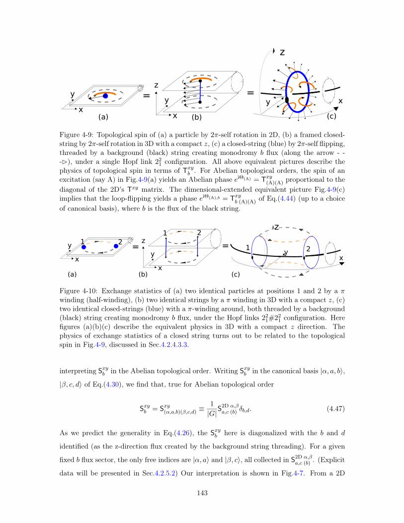
x
y
z
x
z
yx
y
(a) (b) (c)
= =
Figure 4-9: Topological spin of (a) a particle by 2𝜋-self rotation in 2D, (b) a framed closed-string by 2𝜋-self rotation in 3D with a compact 𝑧, (c) a closed-string (blue) by 2𝜋-self flipping,threaded by a background (black) string creating monodromy 𝑏 flux (along the arrow - --B), under a single Hopf link 221 configuration. All above equivalent pictures describe thephysics of topological spin in terms of T𝑥𝑦𝑏 . For Abelian topological orders, the spin of anexcitation (say A) in Fig.4-9(a) yields an Abelian phase 𝑒iΘ(A) = T𝑥𝑦(A)(A) proportional to thediagonal of the 2D’s T𝑥𝑦 matrix. The dimensional-extended equivalent picture Fig.4-9(c)implies that the loop-flipping yields a phase 𝑒iΘ(A),𝑏 = T𝑥𝑦𝑏 (A)(A) of Eq.(4.44) (up to a choiceof canonical basis), where 𝑏 is the flux of the black string.
1 2
x
y
z
yx
z
1 2=
x
y
(a)
=
(b) (c)
1 2
Figure 4-10: Exchange statistics of (a) two identical particles at positions 1 and 2 by a 𝜋winding (half-winding), (b) two identical strings by a 𝜋 winding in 3D with a compact 𝑧, (c)two identical closed-strings (blue) with a 𝜋-winding around, both threaded by a background(black) string creating monodromy 𝑏 flux, under the Hopf links 221#221 configuration. Herefigures (a)(b)(c) describe the equivalent physics in 3D with a compact 𝑧 direction. Thephysics of exchange statistics of a closed string turns out to be related to the topologicalspin in Fig.4-9, discussed in Sec.4.2.4.3.3.
interpreting S𝑥𝑦𝑏 in the Abelian topological order. Writing S𝑥𝑦𝑏 in the canonical basis |𝛼, 𝑎, 𝑏⟩,
|𝛽, 𝑐, 𝑑⟩ of Eq.(4.30), we find that, true for Abelian topological order
S𝑥𝑦𝑏 = S𝑥𝑦(𝛼,𝑎,𝑏)(𝛽,𝑐,𝑑) ≡1
|𝐺|S2D 𝛼,𝛽𝑎,𝑐 (𝑏) 𝛿𝑏,𝑑. (4.47)
As we predict the generality in Eq.(4.26), the S𝑥𝑦𝑏 here is diagonalized with the 𝑏 and 𝑑
identified (as the z-direction flux created by the background string threading). For a given
fixed 𝑏 flux sector, the only free indices are |𝛼, 𝑎⟩ and |𝛽, 𝑐⟩, all collected in S2D 𝛼,𝛽𝑎,𝑐 (𝑏) . (Explicit
data will be presented in Sec.4.2.5.2) Our interpretation is shown in Fig.4-7. From a 2D
143
viewpoint, S𝑥𝑦𝑏 gives the full 2𝜋 braiding statistics data of two quasiparticle |𝛼, 𝑎⟩ and |𝛽, 𝑐⟩
excitations in Fig.4-7(a). However, from the 3D viewpoint, the two particles are actually
two closed strings compactified along the compact 𝑧 direction. Thus, the full-2𝜋 braiding of
two particles in Fig.4-7(a) becomes that of two closed-strings in Fig.4-7(b). More explicitly,
an equivalent 3D view in Fig.4-7(c), we identify the coordinates 𝑥, 𝑦, 𝑧 carefully to see such a
full-braiding process is that one (red) string going inside to the loop of another (blue) string,
and then going back from the outside.
The above picture works again for both the 𝑏 = 0 zero flux sector as well as the 𝑏 = 0 sec-
tor under the background string threading. When 𝑏 = 0, the third (black) background string
in Fig.4-7(c) threading through the two (red, blue) strings. The third (black) string creates
the monodromy defect/branch cut on the background, and carrying 𝑏 flux along 𝑧 acting on
two (red, blue) strings which have nontrivial winding on the third string. This three-string
braiding was first emphasized in a recent paper,[76] here we make further connection to the
data S𝑥𝑦𝑏 and understand its physics in a 3D to 2D under 𝑏 flux sectors.
We have proposed and shown that S𝑥𝑦𝑏 can capture the physics of three-
string braiding statistics with two strings threaded by a third background string
causing 𝑏 flux monodromy, where the three strings have the linking configuration
as the connected sum of two Hopf links 221#221.
4.2.4.3.3 Spin-Statistics relation for closed strings Since a spin-statistics relation
for 2D particles is shown by Fig.4-8, we may wonder, by using our 3D to 2D reduction
picture, whether a spin-statistics relation for a closed string holds?
To answer this question, we should compare the topological spin picture of T𝑥𝑦𝑏 = T𝑎𝑦 ,𝑏𝑧𝛼𝑥
≡ exp(iΘ𝑎𝑦 ,𝑏𝑧𝛼𝑥 ) to the exchange statistic picture of two closed strings in Fig.4-10. Fig.4-10
essentially takes a half-braiding of the S𝑥𝑦𝑏 process of Fig.4-7, and considers doing half-
braiding on the same excitations in |𝛼, 𝑎, 𝑏⟩ = |𝛽, 𝑐, 𝑑⟩. In principle, one can generalize
the framed worldline picture of particles in Fig.4-8 to the framed worldsheet picture of
closed-strings. (ps. The framed worldline is like a worldsheet, the framed worldsheet is
like a worldvolume.) This interpretation shows that the topological spin of Fig.4-9 and the
exchange statistics of Fig.4-10 carry the same data, namely
T𝑥𝑦𝑏 = T𝑎𝑦 ,𝑏𝑧𝛼𝑥 = (S2D 𝛼𝑥,𝛼𝑥
𝑎𝑦 ,𝑎𝑦 (𝑏𝑧))12 or (S2D 𝛼𝑥,𝛼𝑥
𝑎𝑦 ,𝑎𝑦 (𝑏𝑧))12* (4.48)
144
from the data of Eq.(4.44),(4.47). The equivalence holds, up to a (complex conjugate *) sign
caused by the orientation of the rotation and the exchange.
In Sec.(4.2.5.2), we will show, for the twisted gauge theory of Abelian topological orders,
such an interpretation Eq.4.48 is correct and agrees with our data. We term this as the
spin-statistics relation for a closed string.
In this section, we have obtained the explicit formulas of S𝑥𝑦𝑧, T𝑥𝑦, S𝑥𝑦 in Sec.4.2.4.1,4.2.4.2,
and as well as captured the physical meanings of S𝑥𝑦𝑏 , T𝑥𝑦𝑏 in Sec.4.2.4.3.3. Before conclud-
ing, we note that the full understanding of S𝑥𝑦𝑧 seems to be intriguingly related to the 3D
nature. It is not obvious to us that the use of 3D to 2D reduction can capture all physics of
S𝑥𝑦𝑧. We will come back to comment this issue in the Sec.5.3.10.
4.2.5 SL(3,Z) Modular Data and Multi-String Braiding
4.2.5.1 Ground state degeneracy and Particle, String types
We now proceed to study the topology-dependent ground state degeneracy (GSD), modular
data S, T of 3+1D twisted gauge theory with finite group 𝐺 =∏𝑖 𝑍𝑁𝑖 . We shall comment
that the GSD on T2 of 2D topological order counts the number of quasi-particle excitations,
which from the Representation (Rep) Theory is simply counting the number of charges 𝛼
and fluxes 𝑎 forming the quasi-particle basis |𝛼, 𝑎⟩ spanned the ground state Hilbert space.
In 2D, GSD counts the number of types of quasi-particles (or anyons) as well as
the number of basis |𝛼, 𝑎⟩. For higher dimension, GSD on T𝑑 of 𝑑-D topological order
still counts the number of canonical basis |𝛼, 𝑎, 𝑏, . . . ⟩, however, may over count the
number of types of particles (with charge), strings (with flux), etc excitations. From
a untwisted 𝑍𝑁 field theory perspective, the fluxed string may be described by a 2-form
𝐵 field, and the charged particle may be described by a 1-form 𝐴 field, with a BF action∫𝐵𝑑𝐴. As we can see the fluxes 𝑎, 𝑏 are over-counted.
We suggest that counting the number of types of particles of 𝑑-dimensions is equivalent
to Fig.4-11 process, where we dig a ball 𝐵𝑑 with a sphere 𝑆𝑑−1 around the particle 𝑞,
which resides on 𝑆𝑑. And we connect it through a 𝑆1 tunnel to its anti-particle 𝑞. This
process causes creation-annihilation from vacuum, and counts how many types of 𝑞 sectors
145
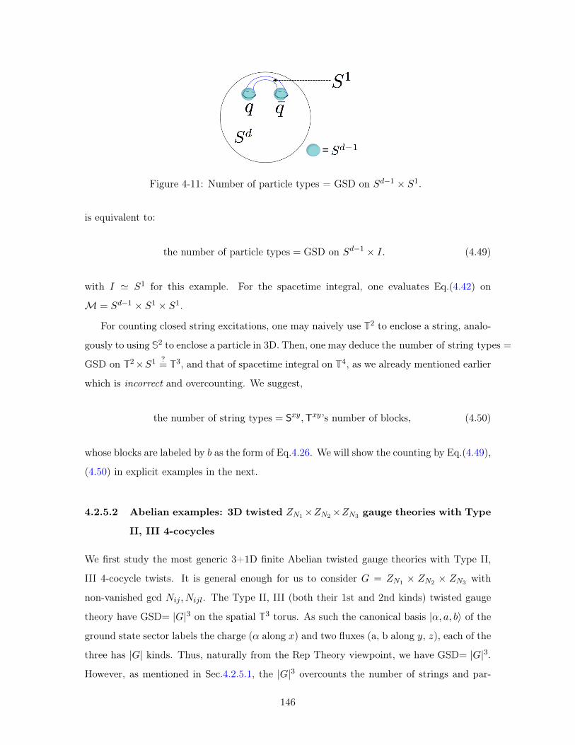
=
Figure 4-11: Number of particle types = GSD on 𝑆𝑑−1 × 𝑆1.
is equivalent to:
the number of particle types = GSD on 𝑆𝑑−1 × 𝐼. (4.49)
with 𝐼 ≃ 𝑆1 for this example. For the spacetime integral, one evaluates Eq.(4.42) on
ℳ = 𝑆𝑑−1 × 𝑆1 × 𝑆1.
For counting closed string excitations, one may naively use T2 to enclose a string, analo-
gously to using S2 to enclose a particle in 3D. Then, one may deduce the number of string types =
GSD on T2×𝑆1 ?= T3, and that of spacetime integral on T4, as we already mentioned earlier
which is incorrect and overcounting. We suggest,
the number of string types = S𝑥𝑦,T𝑥𝑦’s number of blocks, (4.50)
whose blocks are labeled by 𝑏 as the form of Eq.4.26. We will show the counting by Eq.(4.49),
(4.50) in explicit examples in the next.
4.2.5.2 Abelian examples: 3D twisted 𝑍𝑁1×𝑍𝑁2×𝑍𝑁3 gauge theories with Type
II, III 4-cocycles
We first study the most generic 3+1D finite Abelian twisted gauge theories with Type II,
III 4-cocycle twists. It is general enough for us to consider 𝐺 = 𝑍𝑁1 × 𝑍𝑁2 × 𝑍𝑁3 with
non-vanished gcd 𝑁𝑖𝑗 , 𝑁𝑖𝑗𝑙. The Type II, III (both their 1st and 2nd kinds) twisted gauge
theory have GSD= |𝐺|3 on the spatial T3 torus. As such the canonical basis |𝛼, 𝑎, 𝑏⟩ of the
ground state sector labels the charge (𝛼 along 𝑥) and two fluxes (a, b along 𝑦, 𝑧), each of the
three has |𝐺| kinds. Thus, naturally from the Rep Theory viewpoint, we have GSD= |𝐺|3.
However, as mentioned in Sec.4.2.5.1, the |𝐺|3 overcounts the number of strings and par-
146
ticles. By using Eq.(4.49),(4.50), we find there are |𝐺| types of particles and |𝐺| types of
strings. The canonical basis |𝛼, 𝑎, 𝑏⟩ (GSD on T3) counts twice the flux sectors. Several
remarks follow:
(1) For an untwisted gauge theory (topological term 𝑝.. = 0), which is the direct product of
𝑍𝑁 gauge theory or 𝑍𝑁 toric code, its statistics has the form exp(∑𝑘
2𝜋i𝑁𝑘
(𝛽𝑘𝑎𝑘−𝛼𝑘𝑑𝑘))
and
exp(∑𝑘
2𝜋i𝑁𝑘
𝛼𝑘 · 𝑎𝑘). This shall be described by the BF theory of
∫𝐵𝑑𝐴 action. With 𝛼, 𝛽
as the charge of particles (1-form gauge field 𝐴), 𝑎, 𝑏 as the flux of string(2-form gauge field
𝐵). This essentially describes the braiding between a pure-particle and a pure-string.
(2) Both S𝑥𝑦, T𝑥𝑦 have block diagonal forms as S𝑥𝑦𝑏 , T𝑥𝑦𝑏 respect to the 𝑏 flux (along 𝑧)
correctly reflects what Eq.(4.26) preludes already.
(3) T𝑥𝑦 is in SL(3,Z) canonical basis automatically and full-diagonal, but S𝑥𝑦 may not be in
the canonical basis for each blocks of S𝑥𝑦𝑏 , due to its SL(2,Z) nature. We can find the proper
basis in each 𝑏 block. Nevertheless, the eigenvalues of S𝑥𝑦 are still proper and invariant
regardless any basis.
(4) Characterization of topological orders: We can further compare the 3D S𝑥𝑦𝑏 data
to SL(2,Z)’s data of 2D S𝑥𝑦 of ℋ3(𝐺,R/Z). All of the dimensional reduction of these data
(S𝑥𝑦𝑏 and T𝑥𝑦𝑏 ) agree with 3-cocycle (induced from 4-cocycle 𝜔4). Gathering all data, we
conclude that Eq.(4.38) becomes explicitly. For example, Type II twists for 𝐺 = (𝑍2)2 as,
𝒞3D(𝑍2)2,1= 4𝒞2D(𝑍2)2,1
(4.51)
𝒞3D(𝑍2)2, 𝜔4,II = 𝒞2D(𝑍2)2
⊕ 𝒞2D(𝑍2)2,𝜔3,I⊕ 2𝒞2D(𝑍2)2,𝜔3,II
(4.52)
Such a Type II 𝜔4,II can produce a 𝑏 = 0 sector of (𝑍2 toric code ⊗ 𝑍2 toric code) of 2D as
𝒞2D(𝑍2)2, some 𝑏 = 0 sector of (𝑍2 double-semions ⊗ 𝑍2 toric code) as 𝒞2D(𝑍2)2,𝜔3,I
and another
𝑏 = 0 sector 𝒞2D(𝑍2)2,𝜔3,II, for example. This procedure can be applied to other types of cocycle
twists.
(5) Classification of topological orders:
We shall interpret the decomposition in Eq.(4.38) as the implication of classification. Let
147
us do the counting of number of phases in the simplest example of Type II, 𝐺 = 𝑍2 × 𝑍2
twisted theory. There are four types in (𝑝(1𝑠𝑡)II(12), 𝑝
2𝑛𝑑II(12)) ∈ ℋ
4(𝐺,R/Z) = (Z2)2. However,
we find there are only two distinct topological orders out of four. One is the trivial
(𝑍2)2 gauge theory as Eq.(4.51), the other is the nontrivial type as Eq.(4.52). There are
two ways to see this, (i) from the full S𝑥𝑦𝑧, T𝑥𝑦 data. (ii) viewing the sector of S𝑥𝑦𝑏 , T𝑥𝑦𝑏under distinct fluxes 𝑏, which is from a ℋ3(𝐺,R/Z) perspective. We should beware that in
principle tagging particles, strings or gauge groups is not allowed, so one can identify many
seemingly-different orders by relabeling their excitations.
(6) Spin-statistics relation of closed strings in Eq.(4.48) is verified to be correct here,
while we take the complex conjugate in Eq.(4.48). This is why we draw the orientation of
Fig.4-9,4-10 oppositely. Interpreting T𝑥𝑦 as the topological spin also holds.
(7) Cyclic relation for S𝑥𝑦𝑧 in 3D: For all the above data (Type II, Type III), there is a
special cyclic relation for S𝛼,𝛽𝑎,𝑏,𝑑 when the charge labels are equal 𝛼 = 𝛽 (e.g. for pure fluxes
𝛼 = 𝛽 = 0, namely for pure strings):
S𝛼,𝛼𝑎,𝑏,𝑑 · S𝛼,𝛼𝑏,𝑑,𝑎 · S
𝛼,𝛼𝑑,𝑎,𝑏 = 1. (4.53)
However, such a cyclic relation does not hold (even at the zero charge) for S2D 𝛼,𝛽𝑎,𝑐 (𝑏) , namely
S2D 𝛼,𝛽𝑎,𝑐 (𝑏) · S
2D 𝛼,𝛽𝑐,𝑏 (𝑎) · S
2D 𝛼,𝛽𝑏,𝑎 (𝑐) = 1 in general. Some other cyclic relations are studied recently in
Ref.[105, 106], for which we have not yet made detailed comparisons but the perspectives
may be different. In Ref.[106], their cyclic relation is determined by triple linking numbers
associated with the membrane operators. In Ref.[105], their cyclic relation is related to the
loop braiding of Fig.4-7, which has its relevancy instead to S2D 𝛼,𝛽𝑎,𝑐 (𝑏) , not our cyclic relation
of S𝛼,𝛽𝑎,𝑏,𝑑 for 3D.
4.2.5.3 Non-Abelian examples: 3D twisted (𝑍𝑛)4 gauge theories with Type IV
4-cocycle
We now study a more interesting example, a generic 3+1D finite Abelian twisted gauge
theory with Type IV 4-cocycle twists with 𝑝𝑖𝑗𝑙𝑚 = 0. For generality, our formula also
incorporates Type IV twists together with the aforementioned Type II, III twists. So all
4-cocycle twists will be discussed in this subsection. Differ from the previous example of
148
Abelian topological order with Abelian statistics in Sec.4.2.5.2, we will show Type IV 4-
cocycle 𝜔4,IV will cause the gauge theory becomes non-Abelian, having non-Abelian statistics
even if the original 𝐺 is Abelian. Our inspiration rooted in a 2D example for Type III
3-cocycle twist will cause a similar effect, discovered in Ref.[96]. In general, one can con-
sider 𝐺 = 𝑍𝑁1 × 𝑍𝑁2 × 𝑍𝑁3 × 𝑍𝑁4 with non-vanished gcd 𝑁1234; however, we will focus on
𝐺 = (𝑍𝑛)4 with 𝑁1234 = 𝑛, with 𝑛 is prime for simplicity. From ℋ4(𝐺,R/Z) = Z21
𝑛 , we have
𝑛21 types of theories, while 𝑛20 are Abelian gauge theories, and 𝑛20 · (𝑛−1) types with Type
IV 𝜔4 show non-Abelian statistics.
Ground state degeneracy (GSD)-
We compute the GSD of gauge theories with a Type IV twist on the spatial T3 torus,
truncated from = |𝐺|3 = |𝑛4|3 = 𝑛12 to:
GSDT3,IV =(𝑛8 + 𝑛9 − 𝑛5
)+
(𝑛10 − 𝑛7 − 𝑛6 + 𝑛3
)(4.54)
≡ GSD𝐴𝑏𝑒𝑙T3,IV + GSD𝑛𝐴𝑏𝑒𝑙
T3,IV (4.55)
(We derive the above only for a prime 𝑛. The GSD truncation is less severe and is in between
GSDT3,IV and |𝐺|3 for a non-prime 𝑛.) As such, the canonical basis |𝛼, 𝑎, 𝑏⟩ of the ground
state sector on T3 no longer has |𝐺|3 labels with the |𝐺| number charge and two pairs of |𝐺|×
|𝐺| number of fluxes as in Sec.4.2.5.2. This truncation is due to the nature of non-Abelian
physics of Type IV 𝜔4,IV twisted. We explain our notation in Eq.(4.55); the (𝑛)𝐴𝑏𝑒𝑙 indicates
the contribution from (non-)Abelian excitations. From the Rep Theory viewpoint, we can
recover the truncation back to |𝐺|3 by carefully reconstructing the quantum dimension of
excitations. We obtain
|𝐺|3 =(GSD𝐴𝑏𝑒𝑙
T3,IV)+(GSD𝑛𝐴𝑏𝑒𝑙
T3,IV)· 𝑛2 (4.56)
= {𝑛4 + 𝑛5 − 𝑛} · 𝑛4 · (1)2+{(𝑛4)2 − 𝑛5 − 𝑛4 + 𝑛} · 𝑛2 · (𝑛)2
= {Flux𝐴𝑏𝑒𝑙IV } · 𝑛4 · (dim1)2 + {Flux𝑛𝐴𝑏𝑒𝑙IV } · 𝑛2 · (dim𝑛)
2
The dim𝑚 means the dimension of Rep as dim(Rep) is 𝑚, which is also the quantum di-
mension of excitations. Here we have a dimension 1 for Abelian and 𝑛 for non-Abelian.
In summary, we understand the decomposition precisely in terms of each (non-)Abelian
149
contribution as follows:⎧⎪⎪⎪⎪⎪⎪⎨⎪⎪⎪⎪⎪⎪⎩
flux sectors = |𝐺|2 = |𝑛4|2 = Flux𝐴𝑏𝑒𝑙IV + Flux𝑛𝐴𝑏𝑒𝑙IV
GSDT3,IV = GSD𝐴𝑏𝑒𝑙T3,IV + GSD𝑛𝐴𝑏𝑒𝑙
T3,IV
dim(Rep)2 = 12, 𝑛2
Numbers of charge Rep = 𝑛4, 𝑛2.
(4.57)
Actually, the canonical basis |𝛼, 𝑎, 𝑏⟩ (GSD on T3) still works, the sum of Abelian Flux𝐴𝑏𝑒𝑙IV
and non-Abelian Flux𝑛𝐴𝑏𝑒𝑙IV counts the flux number of 𝑎, 𝑏 as the unaltered |𝐺|2. The charge
Rep 𝛼 is unchanged with a number of |𝐺| = 𝑛4 for Abelian sector with a rank-1 matrix
(1-dim linear or projective) representation, however, the charge Rep 𝛼 is truncated to a
smaller number 𝑛2 for non-Abelian sector also with a larger rank-n matrix (n-dim projective)
representation.
Another view on GSDT3,IV can be inspired by a generic formula like Eq.(4.26)
GSDℳ′×𝑆1 = ⊕𝑏GSD𝑏,ℳ′ =∑𝑏
GSD𝑏,ℳ′ , (4.58)
where we sum over GSD in all different 𝑏 flux sectors, with 𝑏 flux along 𝑆1. Here we can
take ℳ′ × 𝑆1 = T3 and ℳ′ = T2. For non-Type IV (untwisted, Type II, III) 𝜔4 case, we
have |𝐺| sectors of 𝑏 flux and each has GSD𝑏,T2 = |𝐺|2. For Type IV 𝜔4 case 𝐺 = (𝑍𝑛)4
with a prime 𝑛, we have
GSDT3,IV = |𝐺|2 + (|𝐺| − 1) · |𝑍𝑛|2 · (1 · |𝑍𝑛|3 + (|𝑍𝑛|2 − 1) · 𝑛)
= 𝑛8 + (𝑛4 − 1) · 𝑛2 · (1 · 𝑛3 + (𝑛3 − 1) · 𝑛). (4.59)
As we expect, the first part is from the zero flux 𝑏 = 0, which is the normal untwisted 2+1D
(𝑍𝑛)4 gauge theory (toric code) as 𝒞2𝐷(𝑍𝑛)4
with |𝐺|2 = 𝑛8 on 2-torus. The remaining (|𝐺|−1)
copies are inserted with nonzero flux (𝑏 = 0) as 𝒞2𝐷(𝑍𝑛)4,𝜔3with Type III 3-cocycle twists of
Table ??. In some case but not all cases, 𝒞2𝐷(𝑍𝑛)4,𝜔3is 𝒞2𝐷
(𝑍𝑛)untwist×(𝑍𝑛)3twist,𝜔3. In either case,
the GSD𝑏,T2 for 𝑏 = 0 has the same decomposition always equivalent to a untwisted 𝑍𝑛
gauge theory with 𝐺𝑆𝐷T2 = 𝑛2 direct product with
GSDT2,𝜔3,III = (1 · 𝑛3 + (𝑛3 − 1) · 𝑛) ≡ GSD𝐴𝑏𝑒𝑙T2,𝜔3,III
+ GSD𝑛𝐴𝑏𝑒𝑙T2,𝜔3,III
, (4.60)
150
which we generalize the result derived for 2+1D Type III 𝜔3 twisted theory with 𝐺 = (𝑍2)3
in Ref.[96] to 𝐺 = (𝑍𝑛)3 of a prime 𝑛.
To summarize, from the GSD counting, we already foresee there exist non-Abelian
strings in 3+1D Type IV twisted gauge theory, with a quantum dimension 𝑛.
Those non-Abelian strings (fluxes) carries dim(Rep) = 𝑛 non-Abelian charges. Since charges
are sourced by particles, those non-Abelian strings are not pure strings but attached
with non-Abelian particles. (For a projection perspective from 3D to 2D, a nonAbelain
string of 𝒞3D is a non-Abelain dyon with both charge and flux of 𝒞2D𝑏 .)
Some remarks follow:
(1) Dimensional reduction from 3D to 2D sectors with 𝑏 flux: From the above
S𝑥𝑦𝑧,T𝑥𝑦, there is no difficulty deriving S𝑥𝑦 from Eq.(4.45). From all these modular data
S𝑥𝑦𝑏 ,T𝑥𝑦𝑏 data, we find consistency with the dimensional reduction of 3D topological order
by comparison with induced 3-cocycle 𝜔3 from 𝜔4. Let us consider a single specific example,
given the Type IV 𝑝1234 = 1 and other zero Type II,III indices 𝑝.. = 𝑝... = 0,
𝒞3D(𝑍2)4,𝜔4,IV= ⊕𝑏𝒞2D𝑏 = 𝒞2D(𝑍2)4
⊕ 10 𝒞2D(𝑍2)×(𝑍2)3(𝑖𝑗𝑙),𝜔
(𝑖𝑗𝑙)3,III⊕ 5𝒞2D(𝑍2)4,𝜔3,III×𝜔3,III×...
= 𝒞2D(𝑍2)4⊕ 10 𝒞2D(𝑍2)×(𝐷4)
⊕ 5𝒞2D(𝑍2)4,𝜔3,III×𝜔3,III×...
The 𝒞2D(𝑍2)4again is the normal (𝑍2)
4 gauge theory at 𝑏 = 0. The 10 copies of 𝒞2D(𝑍2)×(𝐷4)
have an untwisted dihedral 𝐷4 gauge theory (|𝐷4| = 8) product with the normal (𝑍2) gauge
theory. The duality to 𝐷4 theory in 2D can be expected,[107] see Table 4.2. (As a byproduct
of our work, we go beyond Ref.[107] to give the complete classification of all twisted 2D 𝜔3 of
𝐺 = (𝑍2)3 and their corresponding topological orders and twisted quantum double 𝐷𝜔(𝐺)
in Appendices of [52].) The remaining 5 copies 𝒞2D(𝑍2)4,𝜔3,III×𝜔3,III×... must contain the twist
on the full group (𝑍2)4, not just its subgroup. This peculiar feature suggests the following
remark.
(2) Sometimes there may exist a duality between a twisted Abelian gauge theory and a
untwisted non-Abelian gauge theory,[107] one may wonder whether one can find a dual non-
Abelian gauge theory for 𝒞3D(𝑍2)4,𝜔4,IV? We find that, however, 𝒞3D(𝑍2)4,𝜔4,IV
cannot be dual
to a normal gauge theory (neither Abelian nor non-Abelian), but must be a
twisted (Abelian or non-Abelian) gauge theory. The reason is more involved. Let us
151
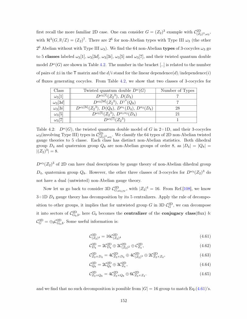
first recall the more familiar 2D case. One can consider 𝐺 = (𝑍2)3 example with 𝒞2D(𝑍2)3,𝜔3
,
with ℋ3(𝐺,R/Z) = (Z2)7. There are 26 for non-Abelian types with Type III 𝜔3 (the other
26 Abelian without with Type III 𝜔3). We find the 64 non-Abelian types of 3-cocycles 𝜔3 go
to 5 classes labeled 𝜔3[1], 𝜔3[3𝑑], 𝜔3[3𝑖], 𝜔3[5] and 𝜔3[7], and their twisted quantum double
model 𝐷𝜔(𝐺) are shown in Table 4.2. The number in the bracket [..] is related to the number
of pairs of ±i in the T matrix and the 𝑑/𝑖 stand for the linear dependence(𝑑)/independence(𝑖)
of fluxes generating cocycles. From Table 4.2, we show that two classes of 3-cocycles for
Class Twisted quantum double 𝐷𝜔(𝐺) Number of Types𝜔3[1] 𝐷𝜔3[1](𝑍2
3), 𝐷(𝐷4) 7𝜔3[3𝑑] 𝐷𝜔3[3𝑑](𝑍2
3), 𝐷𝛾4(𝑄8) 7𝜔3[3𝑖] 𝐷𝜔3[3𝑖](𝑍2
3), 𝐷(𝑄8), 𝐷𝛼1(𝐷4), 𝐷𝛼2(𝐷4) 28𝜔3[5] 𝐷𝜔3[5](𝑍2
3), 𝐷𝛼1𝛼2(𝐷4) 21𝜔3[7] 𝐷𝜔3[7](𝑍2
3) 1
Table 4.2: 𝐷𝜔(𝐺), the twisted quantum double model of 𝐺 in 2+1D, and their 3-cocycles𝜔3(involving Type III) types in 𝒞2D(𝑍2)3,𝜔3
. We classify the 64 types of 2D non-Abelian twistedgauge theories to 5 classe. Each class has distinct non-Abelian statistics. Both dihedralgroup 𝐷4 and quaternion group 𝑄8 are non-Abelian groups of order 8, as |𝐷4| = |𝑄8| =|(𝑍2)
3| = 8.
𝐷𝜔3(𝑍2)3 of 2D can have dual descriptions by gauge theory of non-Abelian dihedral group
𝐷4, quaternion group 𝑄8. However, the other three classes of 3-cocycles for 𝐷𝜔3(𝑍2)3 do
not have a dual (untwisted) non-Abelian gauge theory.
Now let us go back to consider 3D 𝒞3D𝐺,𝜔4,IV, with |𝑍2|4 = 16. From Ref.[108], we know
3+1D 𝐷4 gauge theory has decomposition by its 5 centralizers. Apply the rule of decompo-
sition to other groups, it implies that for untwisted group 𝐺 in 3D 𝒞3D𝐺 , we can decompose
it into sectors of 𝒞2D𝐺𝑏,𝑏, here 𝐺𝑏 becomes the centralizer of the conjugacy class(flux) 𝑏:
𝒞3D𝐺 = ⊕𝑏𝒞2D𝐺𝑏,𝑏. Some useful information is:
𝒞3D(𝑍2)4= 16𝒞2D(𝑍2)4
(4.61)
𝒞3D𝐷4= 2𝒞2D𝐷4
⊕ 2𝒞2D(𝑍2)2⊕ 𝒞2D𝑍4
, (4.62)
𝒞3D𝑍2×𝐷4= 4𝒞2D𝑍2×𝐷4
⊕ 4𝒞2D(𝑍2)3⊕ 2𝒞2D𝑍2×𝑍4
, (4.63)
𝒞3D𝑄8= 2𝒞2D𝑄8
⊕ 3𝒞2D𝑍4, (4.64)
𝒞3D𝑍2×𝑄8= 4𝒞2D𝑍2×𝑄8
⊕ 6𝒞2D𝑍2×𝑍4. (4.65)
and we find that no such decomposition is possible from |𝐺| = 16 group to match Eq.(4.61)’s.
152
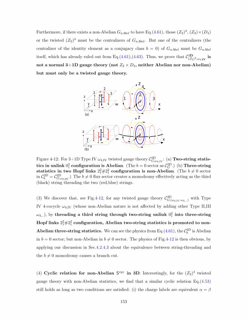
Furthermore, if there exists a non-Abelian 𝐺𝑛𝐴𝑏𝑒𝑙 to have Eq.(4.61), those (𝑍2)4, (𝑍2)×(𝐷4)
or the twisted (𝑍2)4 must be the centralizers of 𝐺𝑛𝐴𝑏𝑒𝑙. But one of the centralizers (the
centralizer of the identity element as a conjugacy class 𝑏 = 0) of 𝐺𝑛𝐴𝑏𝑒𝑙 must be 𝐺𝑛𝐴𝑏𝑒𝑙
itself, which has already ruled out from Eq.(4.61),(4.63). Thus, we prove that 𝒞3D(𝑍2)4,𝜔4,IVis
not a normal 3+1D gauge theory (not 𝑍2 ×𝐷4, neither Abelian nor non-Abelian)
but must only be a twisted gauge theory.
12
34
x
y
zy
x
z
1 3
4
2
=
(a)
x
y
zy
x
z
(b)
=
Figure 4-12: For 3+1D Type IV 𝜔4,IV twisted gauge theory 𝒞3D𝐺,𝜔4,IV: (a) Two-string statis-
tics in unlink 021 configuration is Abelian. (The 𝑏 = 0 sector as 𝒞2D𝐺 .) (b) Three-stringstatistics in two Hopf links 221#221 configuration is non-Abelian. (The 𝑏 = 0 sectorin 𝒞2D𝑏 = 𝒞2D𝐺,𝜔3,III
.) The 𝑏 = 0 flux sector creates a monodromy effectively acting as the third(black) string threading the two (red,blue) strings.
(3) We discover that, see Fig.4-12, for any twisted gauge theory 𝒞3D𝐺,(𝜔4,IV·𝜔4,..)with Type
IV 4-cocycle 𝜔4,IV (whose non-Abelian nature is not affected by adding other Type II,III
𝜔4,..), by threading a third string through two-string unlink 021 into three-string
Hopf links 221#221 configuration, Abelian two-string statistics is promoted to non-
Abelian three-string statistics. We can see the physics from Eq.(4.61), the 𝒞2D𝑏 is Abelian
in 𝑏 = 0 sector; but non-Abelian in 𝑏 = 0 sector. The physics of Fig.4-12 is then obvious, by
applying our discussion in Sec.4.2.4.3 about the equivalence between string-threading and
the 𝑏 = 0 monodromy causes a branch cut.
(4) Cyclic relation for non-Abelian S𝑥𝑦𝑧 in 3D: Interestingly, for the (𝑍2)4 twisted
gauge theory with non-Abelian statistics, we find that a similar cyclic relation Eq.(4.53)
still holds as long as two conditions are satisfied: (i) the charge labels are equivalent 𝛼 = 𝛽
153
and (ii) 𝛿𝑎∈{𝑏,𝑑,𝑏𝑑} · 𝛿𝑑∈{𝑎,𝑏,𝑎𝑏} · 𝛿𝑏∈{𝑑,𝑎,𝑑𝑎} = 1. However, Eq.(4.53) is modified with a factor
depending on the dimensionality of Rep 𝛼:
S𝛼,𝛼𝑎,𝑏,𝑑 · S𝛼,𝛼𝑏,𝑑,𝑎 · S
𝛼,𝛼𝑑,𝑎,𝑏 · |dim(𝛼)|−3 = 1. (4.66)
This identity should hold for any Type IV non-Abelian strings. This is a cyclic relation of
3D nature, instead of a dimensional-reducing 2D nature of S2D 𝛼,𝛽𝑎,𝑐 (𝑏) in Fig.4-7.
So far we had obtain some string-particle braiding identity via the representation theory
and the twisted lattice gauge theory model (of Dijkgraaf-Witten topological gauge theory).
In Chap.6, we will explore more possible identities through another more unified approach:
geometric-topology surgery theory and quantum partition functions.
154
Chapter 5
Aspects of Anomalies
We review chiral fermionic Adler-Bell-Jackiw anomalies and quantum Hall states in Sec.5.1.
The we develop and construct the physical systems with bosonic anomalies in Sec.5.2. We
then attempt to construct a non-perturbative lattice chiral fermion/gauge theory by tackling
the Nielson-Ninomya fermion-doubling no-go theorem in Sec.5.3. With the understanding of
fermionic and bosonic anomalies in topological states of matter, we examine some examples
of mixed gauge-gravity anomalies in Sec.5.4 — by constructing mixed gauge-gravity actions
whose boundaries realize mixed gauge-gravity anomalies. Those mixed gauge-gravity ac-
tions can be regarded as effective probe field actions for SPTs beyond-Group-Cohomology
classification.
5.1 Chiral Fermionic Adler-Bell-Jackiw Anomalies and Topo-
logical Phases
First we present a chiral fermionic anomaly (ABJ anomalies[58, 59]) of a continuous U(1)
symmetry realized in topological phases in condensed matter, in contrast to the bosonic
anomalies of discrete symmetries studied in the next.
Specifically we consider an 1+1D U(1) quantum anomaly realization through 1D edge
of U(1) quantum Hall state, such as in Fig.5-1. We can formulate a Chern-Simons action
𝑆 =∫ (
𝐾4𝜋 𝑎∧ 𝑑𝑎+
𝑞2𝜋𝐴∧ 𝑑𝑎
)with an internal statistical gauge field 𝑎 and an external U(1)
electromagnetic gauge field 𝐴. Its 1+1D boundary is described by a (singlet or multiplet-
)chiral boson theory of a field Φ (Φ𝐿 on the left edge, Φ𝑅 on the right edge). Here the
155
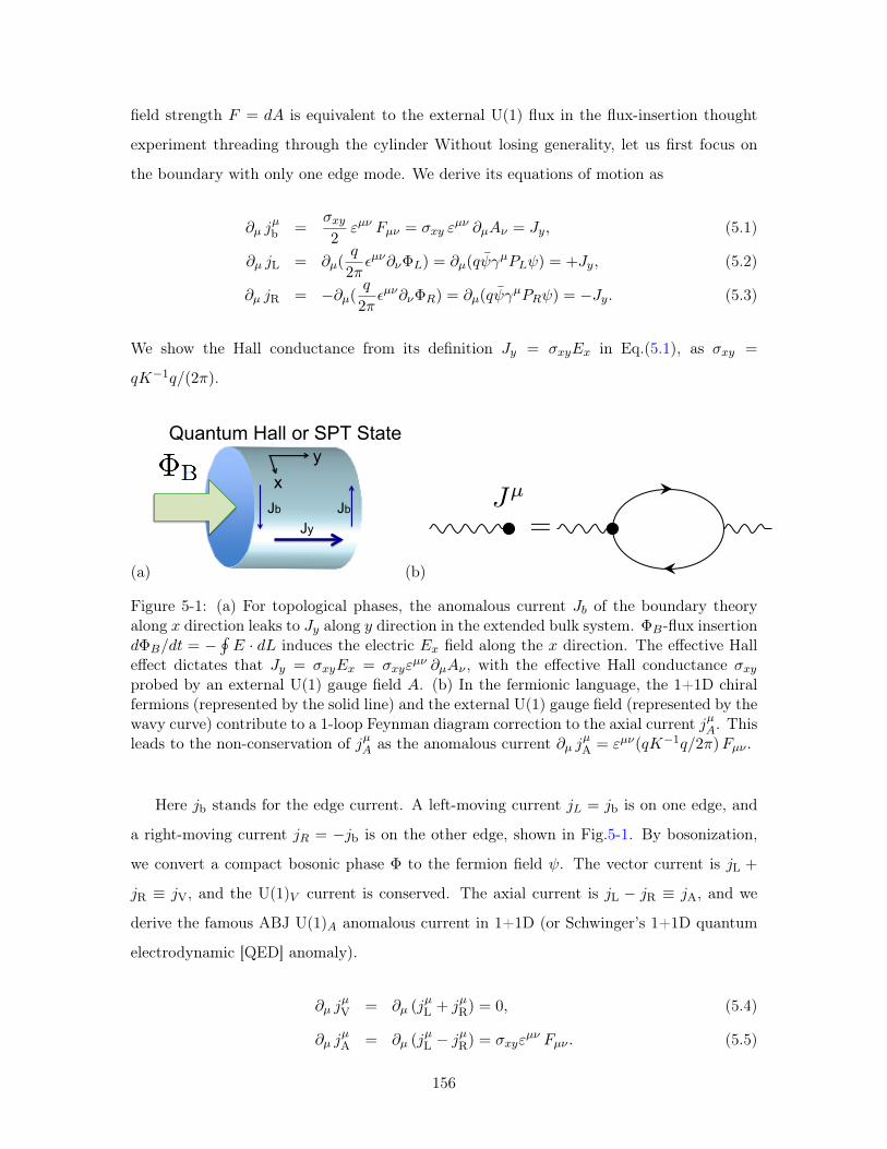
field strength 𝐹 = 𝑑𝐴 is equivalent to the external U(1) flux in the flux-insertion thought
experiment threading through the cylinder Without losing generality, let us first focus on
the boundary with only one edge mode. We derive its equations of motion as
𝜕𝜇 𝑗𝜇b =
𝜎𝑥𝑦2𝜀𝜇𝜈 𝐹𝜇𝜈 = 𝜎𝑥𝑦 𝜀
𝜇𝜈 𝜕𝜇𝐴𝜈 = 𝐽𝑦, (5.1)
𝜕𝜇 𝑗L = 𝜕𝜇(𝑞
2𝜋𝜖𝜇𝜈𝜕𝜈Φ𝐿) = 𝜕𝜇(𝑞𝜓𝛾
𝜇𝑃𝐿𝜓) = +𝐽𝑦, (5.2)
𝜕𝜇 𝑗R = −𝜕𝜇(𝑞
2𝜋𝜖𝜇𝜈𝜕𝜈Φ𝑅) = 𝜕𝜇(𝑞𝜓𝛾
𝜇𝑃𝑅𝜓) = −𝐽𝑦. (5.3)
We show the Hall conductance from its definition 𝐽𝑦 = 𝜎𝑥𝑦𝐸𝑥 in Eq.(5.1), as 𝜎𝑥𝑦 =
𝑞𝐾−1𝑞/(2𝜋).
(a)
y x
Jb Jb Jy
Quantum Hall or SPT State
(b)
Jµ
=
Figure 5-1: (a) For topological phases, the anomalous current 𝐽𝑏 of the boundary theoryalong 𝑥 direction leaks to 𝐽𝑦 along 𝑦 direction in the extended bulk system. Φ𝐵-flux insertion𝑑Φ𝐵/𝑑𝑡 = −
∮𝐸 · 𝑑𝐿 induces the electric 𝐸𝑥 field along the 𝑥 direction. The effective Hall
effect dictates that 𝐽𝑦 = 𝜎𝑥𝑦𝐸𝑥 = 𝜎𝑥𝑦𝜀𝜇𝜈 𝜕𝜇𝐴𝜈 , with the effective Hall conductance 𝜎𝑥𝑦
probed by an external U(1) gauge field 𝐴. (b) In the fermionic language, the 1+1D chiralfermions (represented by the solid line) and the external U(1) gauge field (represented by thewavy curve) contribute to a 1-loop Feynman diagram correction to the axial current 𝑗𝜇𝐴. Thisleads to the non-conservation of 𝑗𝜇𝐴 as the anomalous current 𝜕𝜇 𝑗
𝜇A = 𝜀𝜇𝜈(𝑞𝐾−1𝑞/2𝜋)𝐹𝜇𝜈 .
Here 𝑗b stands for the edge current. A left-moving current 𝑗𝐿 = 𝑗b is on one edge, and
a right-moving current 𝑗𝑅 = −𝑗b is on the other edge, shown in Fig.5-1. By bosonization,
we convert a compact bosonic phase Φ to the fermion field 𝜓. The vector current is 𝑗L +
𝑗R ≡ 𝑗V, and the U(1)𝑉 current is conserved. The axial current is 𝑗L − 𝑗R ≡ 𝑗A, and we
derive the famous ABJ U(1)𝐴 anomalous current in 1+1D (or Schwinger’s 1+1D quantum
electrodynamic [QED] anomaly).
𝜕𝜇 𝑗𝜇V = 𝜕𝜇 (𝑗
𝜇L + 𝑗𝜇R) = 0, (5.4)
𝜕𝜇 𝑗𝜇A = 𝜕𝜇 (𝑗
𝜇L − 𝑗
𝜇R) = 𝜎𝑥𝑦𝜀
𝜇𝜈 𝐹𝜇𝜈 . (5.5)
156
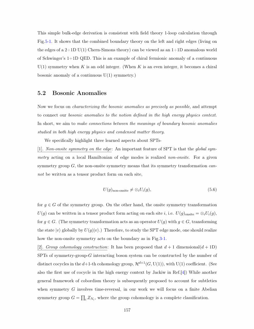
This simple bulk-edge derivation is consistent with field theory 1-loop calculation through
Fig.5-1. It shows that the combined boundary theory on the left and right edges (living on
the edges of a 2+1D U(1) Chern-Simons theory) can be viewed as an 1+1D anomalous world
of Schwinger’s 1+1D QED. This is an example of chiral fermionic anomaly of a continuous
U(1) symmetry when 𝐾 is an odd integer. (When 𝐾 is an even integer, it becomes a chiral
bosonic anomaly of a continuous U(1) symmetry.)
5.2 Bosonic Anomalies
Now we focus on characterizing the bosonic anomalies as precisely as possible, and attempt
to connect our bosonic anomalies to the notion defined in the high energy physics context.
In short, we aim to make connections between the meanings of boundary bosonic anomalies
studied in both high energy physics and condensed matter theory.
We specifically highlight three learned aspects about SPTs-
[1]. Non-onsite symmetry on the edge: An important feature of SPT is that the global sym-
metry acting on a local Hamiltonian of edge modes is realized non-onsite. For a given
symmetry group 𝐺, the non-onsite symmetry means that its symmetry transformation can-
not be written as a tensor product form on each site,
𝑈(𝑔)non-onsite = ⊗𝑖𝑈𝑖(𝑔), (5.6)
for 𝑔 ∈ 𝐺 of the symmetry group. On the other hand, the onsite symmetry transformation
𝑈(𝑔) can be written in a tensor product form acting on each site 𝑖, i.e. 𝑈(𝑔)onsite = ⊗𝑖𝑈𝑖(𝑔),
for 𝑔 ∈ 𝐺. (The symmetry transformation acts as an operator 𝑈(𝑔) with 𝑔 ∈ 𝐺, transforming
the state |𝑣⟩ globally by 𝑈(𝑔)|𝑣⟩.) Therefore, to study the SPT edge mode, one should realize
how the non-onsite symmetry acts on the boundary as in Fig.3-1.
[2]. Group cohomology construction: It has been proposed that 𝑑 + 1 dimensional(𝑑 + 1D)
SPTs of symmetry-group-𝐺 interacting boson system can be constructed by the number of
distinct cocycles in the 𝑑+1-th cohomology group,ℋ𝑑+1(𝐺,U(1)), with U(1) coefficient. (See
also the first use of cocycle in the high energy context by Jackiw in Ref.[4]) While another
general framework of cobordism theory is subsequently proposed to account for subtleties
when symmetry 𝐺 involves time-reversal, in our work we will focus on a finite Abelian
symmetry group 𝐺 =∏𝑖 𝑍𝑁𝑖 , where the group cohomology is a complete classification.
157
[3]. Surface anomalies: It has been proposed that the edge modes of SPTs are the source
of gauge anomalies, while that of intrinsic topological orders are the source of gravitational
anomalies.[49] SPT boundary states are known to show at least one of three properties:
∙(1) symmetry-preserving gapless edge modes,
∙(2) symmetry-breaking gapped edge modes,
∙(3) symmetry-preserving gapped edge modes with surface topological order.
We shall now define the meaning of quantum anomaly in a language appreciable by both
high energy physics and condensed matter communities -
The quantum anomaly is an obstruction of a symmetry of a theory to be fully-regularized for
a full quantum theory as an onsite symmetry on the UV-cutoff lattice in the same spacetime
dimension.According to this definition, to characterize our bosonic anomalies, we will find several pos-
sible obstructions to regulate the symmetry at the quantum level:
⋆ Obstruction of onsite symmetries: Consistently we will find throughout our examples to
fully-regularize our SPTs 1D edge theory on the 1D lattice Hamiltonian requires the non-
onsite symmetry, namely, realizing the symmetry anomalously. The non-onsite symmetry
on the edge cannot be “dynamically gauged” on its own spacetime dimension, thus this also
implies the following obstruction.
⋆ Obstruction of the same spacetime dimension: We will show that the physical observables
for gapless edge modes (the case ∙(1)) are their energy spectral shifts[57] under symmetry-
preserving external flux insertion through a compact 1D ring. The energy spectral shift is
caused by the Laughlin-type flux insertion of Fig.5-2. The flux insertion can be equivalently
regarded as an effective branch cut modifying the Hamiltonian (blue dashed line in Fig.5-
2) connecting from the edge to an extra dimensional bulk. Thus the spectral shifts also
indicate the transportation of quantum numbers from one edge to the other edge. This can
be regarded as the anomaly requiring an extra dimensional bulk.
⋆ Non-perturbative effects: We know that the familiar Adler-Bell-Jackiw anomaly of chiral
fermions,[58, 59] observed in the pion decay in particle-physics can be captured by the
perturbative 1-loop Feynman diagram. However, importantly, the result is non-perturbative,
being exact from low energy IR to high energy UV. This effect can be further confirmed
via Fujikawa’s path integral method non-perturbatively. Instead of the well-known chiral
fermionic anomalies, do we have bosonic anomalies with these non-perturbative effects?
158
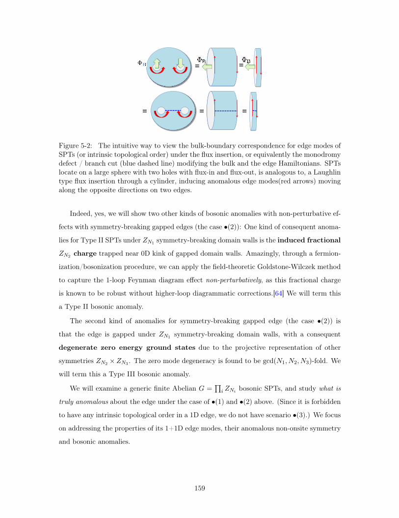
=
= = =
=
Figure 5-2: The intuitive way to view the bulk-boundary correspondence for edge modes ofSPTs (or intrinsic topological order) under the flux insertion, or equivalently the monodromydefect / branch cut (blue dashed line) modifying the bulk and the edge Hamiltonians. SPTslocate on a large sphere with two holes with flux-in and flux-out, is analogous to, a Laughlintype flux insertion through a cylinder, inducing anomalous edge modes(red arrows) movingalong the opposite directions on two edges.
Indeed, yes, we will show two other kinds of bosonic anomalies with non-perturbative ef-
fects with symmetry-breaking gapped edges (the case ∙(2)): One kind of consequent anoma-
lies for Type II SPTs under 𝑍𝑁1 symmetry-breaking domain walls is the induced fractional
𝑍𝑁2 charge trapped near 0D kink of gapped domain walls. Amazingly, through a fermion-
ization/bosonization procedure, we can apply the field-theoretic Goldstone-Wilczek method
to capture the 1-loop Feynman diagram effect non-perturbatively, as this fractional charge
is known to be robust without higher-loop diagrammatic corrections.[64] We will term this
a Type II bosonic anomaly.
The second kind of anomalies for symmetry-breaking gapped edge (the case ∙(2)) is
that the edge is gapped under 𝑍𝑁1 symmetry-breaking domain walls, with a consequent
degenerate zero energy ground states due to the projective representation of other
symmetries 𝑍𝑁2 ×𝑍𝑁3 . The zero mode degeneracy is found to be gcd(𝑁1, 𝑁2, 𝑁3)-fold. We
will term this a Type III bosonic anomaly.
We will examine a generic finite Abelian 𝐺 =∏𝑖 𝑍𝑁𝑖 bosonic SPTs, and study what is
truly anomalous about the edge under the case of ∙(1) and ∙(2) above. (Since it is forbidden
to have any intrinsic topological order in a 1D edge, we do not have scenario ∙(3).) We focus
on addressing the properties of its 1+1D edge modes, their anomalous non-onsite symmetry
and bosonic anomalies.
159
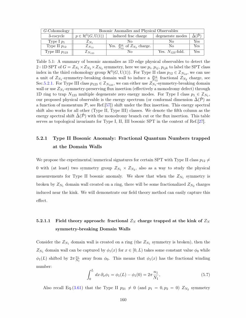
𝐺-Cohomology Bosonic Anomalies and Physical Observables3-cocycle 𝑝 ∈ ℋ3(𝐺,U(1)) induced frac charge degenerate modes Δ(𝒫)Type I 𝑝1 Z𝑁1
No No YesType II 𝑝12 Z𝑁12 Yes. 𝑝12
𝑁12of 𝑍𝑁2 charge. No Yes
Type III 𝑝123 Z𝑁123No Yes. 𝑁123-fold. Yes
Table 5.1: A summary of bosonic anomalies as 1D edge physical observables to detect the2+1D SPT of 𝐺 = 𝑍𝑁1×𝑍𝑁2×𝑍𝑁3 symmetry, here we use 𝑝𝑖, 𝑝𝑖𝑗 , 𝑝𝑖𝑗𝑘 to label the SPT classindex in the third cohomology group ℋ3(𝐺,U(1)). For Type II class 𝑝12 ∈ Z𝑁12 , we can usea unit of 𝑍𝑁1-symmetry-breaking domain wall to induce a 𝑝12
𝑁12fractional 𝑍𝑁2 charge, see
Sec.5.2.1. For Type III class 𝑝123 ∈ Z𝑁123 , we can either use 𝑍𝑁1-symmetry-breaking domainwall or use 𝑍𝑁1-symmetry-preserving flux insertion (effectively a monodromy defect) through1D ring to trap 𝑁123 multiple degenerate zero energy modes. For Type I class 𝑝1 ∈ Z𝑁1 ,our proposed physical observable is the energy spectrum (or conformal dimension Δ(𝒫) asa function of momentum 𝒫, see Ref.[57]) shift under the flux insertion. This energy spectralshift also works for all other (Type II, Type III) classes. We denote the fifth column as theenergy spectral shift Δ(𝒫) with the monodromy branch cut or the flux insertion. This tableserves as topological invariants for Type I, II, III bosonic SPT in the context of Ref.[27].
5.2.1 Type II Bosonic Anomaly: Fractional Quantum Numbers trapped
at the Domain Walls
We propose the experimental/numerical signatures for certain SPT with Type II class 𝑝12 =
0 with (at least) two symmetry group 𝑍𝑁1 × 𝑍𝑁2 , also as a way to study the physical
measurements for Type II bosonic anomaly. We show that when the 𝑍𝑁1 symmetry is
broken by 𝑍𝑁1 domain wall created on a ring, there will be some fractionalized 𝑍𝑁2 charges
induced near the kink. We will demonstrate our field theory method can easily capture this
effect.
5.2.1.1 Field theory approach: fractional 𝑍𝑁 charge trapped at the kink of 𝑍𝑁
symmetry-breaking Domain Walls
Consider the 𝑍𝑁1 domain wall is created on a ring (the 𝑍𝑁1 symmetry is broken), then the
𝑍𝑁1 domain wall can be captured by 𝜑1(𝑥) for 𝑥 ∈ [0, 𝐿) takes some constant value 𝜑0 while
𝜑1(𝐿) shifted by 2𝜋 𝑛1𝑁1
away from 𝜑0. This means that 𝜑1(𝑥) has the fractional winding
number: ∫ 𝐿
0𝑑𝑥 𝜕𝑥𝜑1 = 𝜑1(𝐿)− 𝜑1(0) = 2𝜋
𝑛1𝑁1
, (5.7)
Also recall Eq.(3.61) that the Type II 𝑝21 = 0 (and 𝑝1 = 0, 𝑝2 = 0) 𝑍𝑁2 symmetry
160
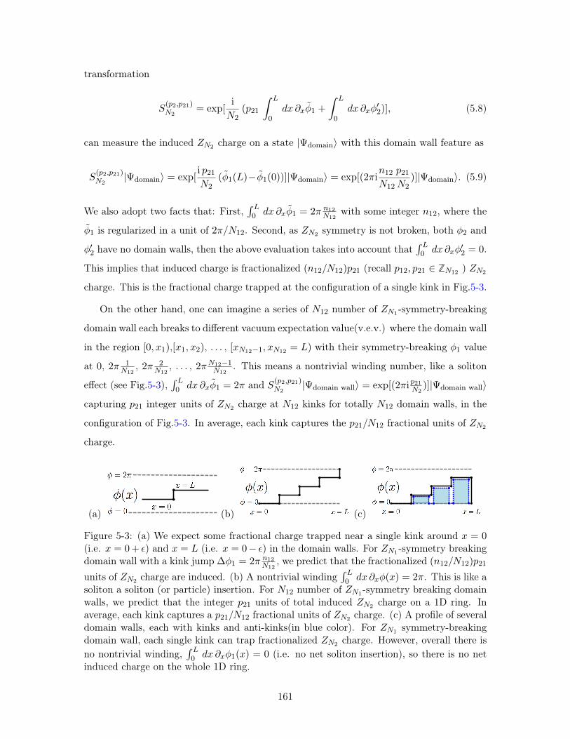
transformation
𝑆(𝑝2,𝑝21)𝑁2
= exp[i𝑁2
(𝑝21
∫ 𝐿
0𝑑𝑥 𝜕𝑥𝜑1 +
∫ 𝐿
0𝑑𝑥 𝜕𝑥𝜑
′2)], (5.8)
can measure the induced 𝑍𝑁2 charge on a state |Ψdomain⟩ with this domain wall feature as
𝑆(𝑝2,𝑝21)𝑁2
|Ψdomain⟩ = exp[i 𝑝21𝑁2
(𝜑1(𝐿)−𝜑1(0))]|Ψdomain⟩ = exp[(2𝜋i𝑛12 𝑝21𝑁12𝑁2
)]|Ψdomain⟩. (5.9)
We also adopt two facts that: First,∫ 𝐿0 𝑑𝑥 𝜕𝑥𝜑1 = 2𝜋 𝑛12
𝑁12with some integer 𝑛12, where the
𝜑1 is regularized in a unit of 2𝜋/𝑁12. Second, as 𝑍𝑁2 symmetry is not broken, both 𝜑2 and
𝜑′2 have no domain walls, then the above evaluation takes into account that∫ 𝐿0 𝑑𝑥 𝜕𝑥𝜑
′2 = 0.
This implies that induced charge is fractionalized (𝑛12/𝑁12)𝑝21 (recall 𝑝12, 𝑝21 ∈ Z𝑁12 ) 𝑍𝑁2
charge. This is the fractional charge trapped at the configuration of a single kink in Fig.5-3.
On the other hand, one can imagine a series of 𝑁12 number of 𝑍𝑁1-symmetry-breaking
domain wall each breaks to different vacuum expectation value(v.e.v.) where the domain wall
in the region [0, 𝑥1),[𝑥1, 𝑥2), . . . , [𝑥𝑁12−1, 𝑥𝑁12 = 𝐿) with their symmetry-breaking 𝜑1 value
at 0, 2𝜋 1𝑁12
, 2𝜋 2𝑁12
, . . . , 2𝜋𝑁12−1𝑁12
. This means a nontrivial winding number, like a soliton
effect (see Fig.5-3),∫ 𝐿0 𝑑𝑥 𝜕𝑥𝜑1 = 2𝜋 and 𝑆(𝑝2,𝑝21)
𝑁2|Ψdomain wall⟩ = exp[(2𝜋i 𝑝21𝑁2
)]|Ψdomain wall⟩
capturing 𝑝21 integer units of 𝑍𝑁2 charge at 𝑁12 kinks for totally 𝑁12 domain walls, in the
configuration of Fig.5-3. In average, each kink captures the 𝑝21/𝑁12 fractional units of 𝑍𝑁2
charge.
(a) (b) (c)
Figure 5-3: (a) We expect some fractional charge trapped near a single kink around 𝑥 = 0(i.e. 𝑥 = 0+ 𝜖) and 𝑥 = 𝐿 (i.e. 𝑥 = 0− 𝜖) in the domain walls. For 𝑍𝑁1-symmetry breakingdomain wall with a kink jump Δ𝜑1 = 2𝜋 𝑛12
𝑁12, we predict that the fractionalized (𝑛12/𝑁12)𝑝21
units of 𝑍𝑁2 charge are induced. (b) A nontrivial winding∫ 𝐿0 𝑑𝑥 𝜕𝑥𝜑(𝑥) = 2𝜋. This is like a
soliton a soliton (or particle) insertion. For 𝑁12 number of 𝑍𝑁1-symmetry breaking domainwalls, we predict that the integer 𝑝21 units of total induced 𝑍𝑁2 charge on a 1D ring. Inaverage, each kink captures a 𝑝21/𝑁12 fractional units of 𝑍𝑁2 charge. (c) A profile of severaldomain walls, each with kinks and anti-kinks(in blue color). For 𝑍𝑁1 symmetry-breakingdomain wall, each single kink can trap fractionalized 𝑍𝑁2 charge. However, overall there isno nontrivial winding,
∫ 𝐿0 𝑑𝑥 𝜕𝑥𝜑1(𝑥) = 0 (i.e. no net soliton insertion), so there is no net
induced charge on the whole 1D ring.
161
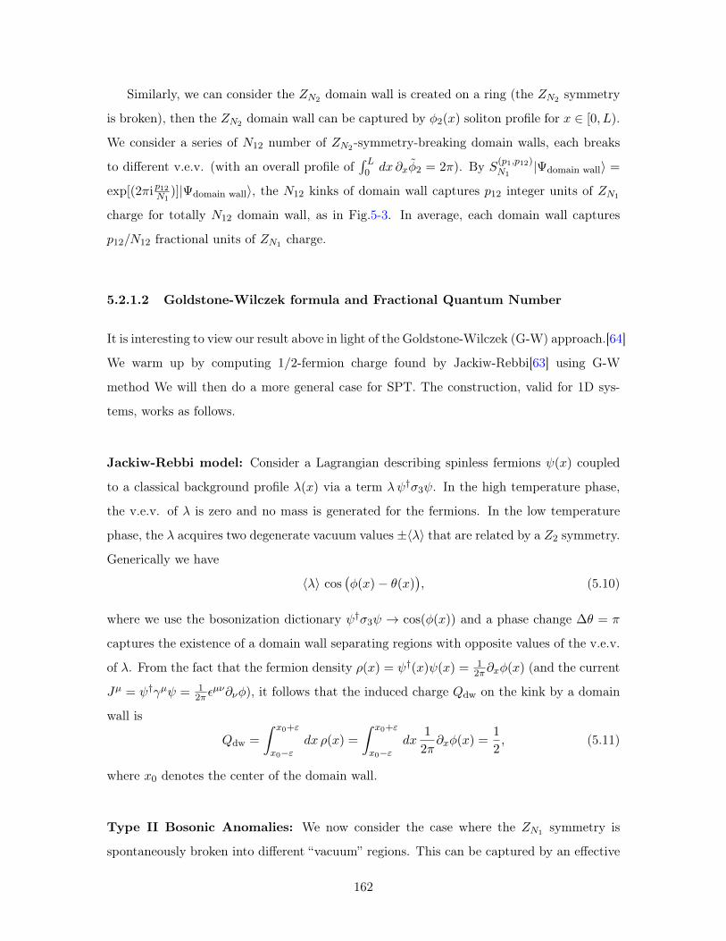
Similarly, we can consider the 𝑍𝑁2 domain wall is created on a ring (the 𝑍𝑁2 symmetry
is broken), then the 𝑍𝑁2 domain wall can be captured by 𝜑2(𝑥) soliton profile for 𝑥 ∈ [0, 𝐿).
We consider a series of 𝑁12 number of 𝑍𝑁2-symmetry-breaking domain walls, each breaks
to different v.e.v. (with an overall profile of∫ 𝐿0 𝑑𝑥 𝜕𝑥𝜑2 = 2𝜋). By 𝑆(𝑝1,𝑝12)
𝑁1|Ψdomain wall⟩ =
exp[(2𝜋i 𝑝12𝑁1)]|Ψdomain wall⟩, the 𝑁12 kinks of domain wall captures 𝑝12 integer units of 𝑍𝑁1
charge for totally 𝑁12 domain wall, as in Fig.5-3. In average, each domain wall captures
𝑝12/𝑁12 fractional units of 𝑍𝑁1 charge.
5.2.1.2 Goldstone-Wilczek formula and Fractional Quantum Number
It is interesting to view our result above in light of the Goldstone-Wilczek (G-W) approach.[64]
We warm up by computing 1/2-fermion charge found by Jackiw-Rebbi[63] using G-W
method We will then do a more general case for SPT. The construction, valid for 1D sys-
tems, works as follows.
Jackiw-Rebbi model: Consider a Lagrangian describing spinless fermions 𝜓(𝑥) coupled
to a classical background profile 𝜆(𝑥) via a term 𝜆𝜓†𝜎3𝜓. In the high temperature phase,
the v.e.v. of 𝜆 is zero and no mass is generated for the fermions. In the low temperature
phase, the 𝜆 acquires two degenerate vacuum values ±⟨𝜆⟩ that are related by a 𝑍2 symmetry.
Generically we have
⟨𝜆⟩ cos(𝜑(𝑥)− 𝜃(𝑥)
), (5.10)
where we use the bosonization dictionary 𝜓†𝜎3𝜓 → cos(𝜑(𝑥)) and a phase change Δ𝜃 = 𝜋
captures the existence of a domain wall separating regions with opposite values of the v.e.v.
of 𝜆. From the fact that the fermion density 𝜌(𝑥) = 𝜓†(𝑥)𝜓(𝑥) = 12𝜋𝜕𝑥𝜑(𝑥) (and the current
𝐽𝜇 = 𝜓†𝛾𝜇𝜓 = 12𝜋 𝜖
𝜇𝜈𝜕𝜈𝜑), it follows that the induced charge 𝑄dw on the kink by a domain
wall is
𝑄dw =
∫ 𝑥0+𝜀
𝑥0−𝜀𝑑𝑥 𝜌(𝑥) =
∫ 𝑥0+𝜀
𝑥0−𝜀𝑑𝑥
1
2𝜋𝜕𝑥𝜑(𝑥) =
1
2, (5.11)
where 𝑥0 denotes the center of the domain wall.
Type II Bosonic Anomalies: We now consider the case where the 𝑍𝑁1 symmetry is
spontaneously broken into different “vacuum” regions. This can be captured by an effective
162
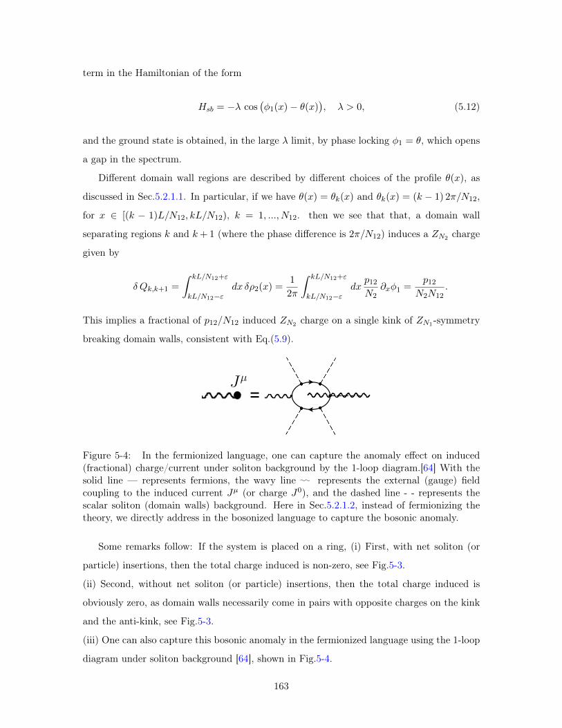
term in the Hamiltonian of the form
𝐻𝑠𝑏 = −𝜆 cos(𝜑1(𝑥)− 𝜃(𝑥)
), 𝜆 > 0, (5.12)
and the ground state is obtained, in the large 𝜆 limit, by phase locking 𝜑1 = 𝜃, which opens
a gap in the spectrum.
Different domain wall regions are described by different choices of the profile 𝜃(𝑥), as
discussed in Sec.5.2.1.1. In particular, if we have 𝜃(𝑥) = 𝜃𝑘(𝑥) and 𝜃𝑘(𝑥) = (𝑘 − 1) 2𝜋/𝑁12,
for 𝑥 ∈ [(𝑘 − 1)𝐿/𝑁12, 𝑘𝐿/𝑁12), 𝑘 = 1, ..., 𝑁12. then we see that that, a domain wall
separating regions 𝑘 and 𝑘+1 (where the phase difference is 2𝜋/𝑁12) induces a 𝑍𝑁2 charge
given by
𝛿 𝑄𝑘,𝑘+1 =
∫ 𝑘𝐿/𝑁12+𝜀
𝑘𝐿/𝑁12−𝜀𝑑𝑥 𝛿𝜌2(𝑥) =
1
2𝜋
∫ 𝑘𝐿/𝑁12+𝜀
𝑘𝐿/𝑁12−𝜀𝑑𝑥
𝑝12𝑁2
𝜕𝑥𝜑1 =𝑝12
𝑁2𝑁12.
This implies a fractional of 𝑝12/𝑁12 induced 𝑍𝑁2 charge on a single kink of 𝑍𝑁1-symmetry
breaking domain walls, consistent with Eq.(5.9).
=
1
I. PLOTS
v1
v2
v4
v3
v′3
FIG. 1: The topology of the action of Agv3 .
g1
g2
g4
g3
g′3
FIG. 2: The topology of the action of Agv3 . Jµ
Figure 5-4: In the fermionized language, one can capture the anomaly effect on induced(fractional) charge/current under soliton background by the 1-loop diagram.[64] With thesolid line — represents fermions, the wavy line :: represents the external (gauge) fieldcoupling to the induced current 𝐽𝜇 (or charge 𝐽0), and the dashed line - - represents thescalar soliton (domain walls) background. Here in Sec.5.2.1.2, instead of fermionizing thetheory, we directly address in the bosonized language to capture the bosonic anomaly.
Some remarks follow: If the system is placed on a ring, (i) First, with net soliton (or
particle) insertions, then the total charge induced is non-zero, see Fig.5-3.
(ii) Second, without net soliton (or particle) insertions, then the total charge induced is
obviously zero, as domain walls necessarily come in pairs with opposite charges on the kink
and the anti-kink, see Fig.5-3.
(iii) One can also capture this bosonic anomaly in the fermionized language using the 1-loop
diagram under soliton background [64], shown in Fig.5-4.
163
(iv) A related phenomena has also been examined recently where fractionalized boundary
excitations cause that the symmetry-broken boundary cannot be proliferated to restore the
symmetry.
5.2.1.3 Lattice approach: Projective phase observed at Domain Walls
Now we would like to formulate a fully regularized lattice approach to derive the induced
fractional charge, and compare to the complementary field theory done in Sec.5.2.1.1 and
Goldstone-Wilczek approach in Sec.5.2.1.2. Recall that in the case of a system with onsite
symmetry, such as 𝑍𝑁 rotor model on a 1D ring with a simple Hamiltonian of∑
𝑗(𝜎𝑗 +𝜎†𝑗),
there is an on-site symmetry transformation 𝑆 =∏𝑗 𝜏𝑗 acting on the full ring. We can
simply take a segment (from the site 𝑟1 to 𝑟2) of the symmetry transformation defined as
a 𝐷 operator 𝐷(𝑟1, 𝑟2) ≡∏𝑟2𝑗=𝑟1
𝜏𝑗 . The 𝐷 operator does the job to flip the measurement
on ⟨𝜎ℓ⟩. What we mean is that ⟨𝜓|𝜎ℓ|𝜓⟩ and ⟨𝜓′|𝜎ℓ|𝜓′⟩ ≡ ⟨𝜓|𝐷†𝜎ℓ𝐷|𝜓⟩ = 𝑒𝑖2𝜋/𝑁 ⟨𝜓|𝜎ℓ|𝜓⟩
are distinct by a phase 𝑒𝑖2𝜋/𝑁 as long as ℓ ∈ [𝑟1, 𝑟2]. Thus 𝐷 operator creates domain wall
profile.
For our case of SPT edge modes with non-onsite symmetry studied here, we are readily
to generalize the above and take a line segment of non-onsite symmetry transformation with
symmetry 𝑍𝑁𝑢 (from the site 𝑟1 to 𝑟2) and define it as a 𝐷𝑁𝑢 operator, 𝐷𝑁𝑢(𝑟1, 𝑟2) ≡∏𝑟2𝑗=𝑟1
𝜏(𝑢)𝑗
∏𝑟2𝑗=𝑟1
𝑈𝑗,𝑗+1𝑊𝐼𝐼𝐼𝑗,𝑗+1 (from the expression of 𝑆𝑁𝑢 , with the onsite piece 𝜏 (𝑢)𝑗 and
the non-onsite piece 𝑈𝑗,𝑗+1 in Eq.(3.48) and 𝑊𝑗,𝑗+1 in Eq.(3.52)). This 𝐷 operator effectively
creates domain wall on the state with a kink (at the 𝑟1) and anti-kink (at the 𝑟2) feature,
such as in Fig.5-3. The total net charge on this type of domain wall (with equal numbers
of kink and anti-kinks) is zero, due to no net soliton insertion (i.e. no net winding, so∫ 𝐿0 𝜕𝑥𝜑𝑑𝑥 = 0). However, by well-separating kinks and anti-kinks, we can still compute
the phase gained at each single kink. We consider the induced charge measurement by
𝑆(𝐷|𝜓⟩), which is (𝑆𝐷𝑆†)𝑆|𝜓⟩ = 𝑒i(Θ0+Θ)𝐷|𝜓⟩, where Θ0 is from the initial charge (i.e.
𝑆|𝜓⟩ ≡ 𝑒iΘ0 |𝜓⟩) and Θ is from the charge gained on the kink. The measurement of symmetry
𝑆 producing a phase 𝑒iΘ, implies a nontrivial induced charge trapped at the kink of domain
walls. We compute the phase at the left kink on a domain wall for all Type I, II, III SPT
classes, and summarize them in Table 5.2.
164
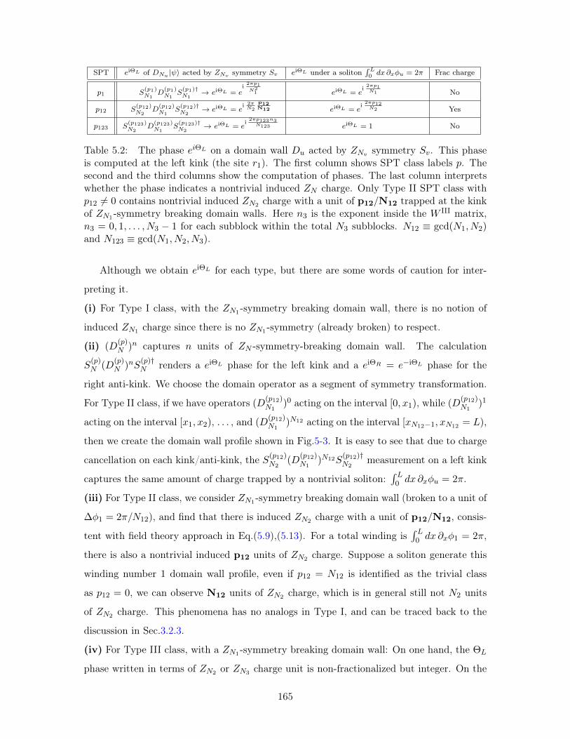
SPT 𝑒iΘ𝐿 of 𝐷𝑁𝑢 |𝜓⟩ acted by 𝑍𝑁𝑣 symmetry 𝑆𝑣 𝑒iΘ𝐿 under a soliton∫ 𝐿0 𝑑𝑥 𝜕𝑥𝜑𝑢 = 2𝜋 Frac charge
𝑝1 𝑆(𝑝1)𝑁1
𝐷(𝑝1)𝑁1
𝑆(𝑝1)†𝑁1
→ 𝑒iΘ𝐿 = 𝑒i 2𝜋𝑝1
𝑁21 𝑒iΘ𝐿 = 𝑒
i 2𝜋𝑝1𝑁1 No
𝑝12 𝑆(𝑝12)𝑁2
𝐷(𝑝12)𝑁1
𝑆(𝑝12)†𝑁2
→ 𝑒iΘ𝐿 = 𝑒i 2𝜋𝑁2
p12N12 𝑒iΘ𝐿 = 𝑒
i 2𝜋𝑝12𝑁2 Yes
𝑝123 𝑆(𝑝123)𝑁2
𝐷(𝑝123)𝑁1
𝑆(𝑝123)†𝑁2
→ 𝑒iΘ𝐿 = 𝑒i 2𝜋𝑝123𝑛3
𝑁123 𝑒iΘ𝐿 = 1 No
Table 5.2: The phase 𝑒𝑖Θ𝐿 on a domain wall 𝐷𝑢 acted by 𝑍𝑁𝑣 symmetry 𝑆𝑣. This phaseis computed at the left kink (the site 𝑟1). The first column shows SPT class labels 𝑝. Thesecond and the third columns show the computation of phases. The last column interpretswhether the phase indicates a nontrivial induced 𝑍𝑁 charge. Only Type II SPT class with𝑝12 = 0 contains nontrivial induced 𝑍𝑁2 charge with a unit of p12/N12 trapped at the kinkof 𝑍𝑁1-symmetry breaking domain walls. Here 𝑛3 is the exponent inside the 𝑊 III matrix,𝑛3 = 0, 1, . . . , 𝑁3 − 1 for each subblock within the total 𝑁3 subblocks. 𝑁12 ≡ gcd(𝑁1, 𝑁2)and 𝑁123 ≡ gcd(𝑁1, 𝑁2, 𝑁3).
Although we obtain 𝑒iΘ𝐿 for each type, but there are some words of caution for inter-
preting it.
(i) For Type I class, with the 𝑍𝑁1-symmetry breaking domain wall, there is no notion of
induced 𝑍𝑁1 charge since there is no 𝑍𝑁1-symmetry (already broken) to respect.
(ii) (𝐷(𝑝)𝑁 )𝑛 captures 𝑛 units of 𝑍𝑁 -symmetry-breaking domain wall. The calculation
𝑆(𝑝)𝑁 (𝐷
(𝑝)𝑁 )𝑛𝑆
(𝑝)†𝑁 renders a 𝑒iΘ𝐿 phase for the left kink and a 𝑒iΘ𝑅 = 𝑒−iΘ𝐿 phase for the
right anti-kink. We choose the domain operator as a segment of symmetry transformation.
For Type II class, if we have operators (𝐷(𝑝12)𝑁1
)0 acting on the interval [0, 𝑥1), while (𝐷(𝑝12)𝑁1
)1
acting on the interval [𝑥1, 𝑥2), . . . , and (𝐷(𝑝12)𝑁1
)𝑁12 acting on the interval [𝑥𝑁12−1, 𝑥𝑁12 = 𝐿),
then we create the domain wall profile shown in Fig.5-3. It is easy to see that due to charge
cancellation on each kink/anti-kink, the 𝑆(𝑝12)𝑁2
(𝐷(𝑝12)𝑁1
)𝑁12𝑆(𝑝12)†𝑁2
measurement on a left kink
captures the same amount of charge trapped by a nontrivial soliton:∫ 𝐿0 𝑑𝑥 𝜕𝑥𝜑𝑢 = 2𝜋.
(iii) For Type II class, we consider 𝑍𝑁1-symmetry breaking domain wall (broken to a unit of
Δ𝜑1 = 2𝜋/𝑁12), and find that there is induced 𝑍𝑁2 charge with a unit of p12/N12, consis-
tent with field theory approach in Eq.(5.9),(5.13). For a total winding is∫ 𝐿0 𝑑𝑥 𝜕𝑥𝜑1 = 2𝜋,
there is also a nontrivial induced p12 units of 𝑍𝑁2 charge. Suppose a soliton generate this
winding number 1 domain wall profile, even if 𝑝12 = 𝑁12 is identified as the trivial class
as 𝑝12 = 0, we can observe N12 units of 𝑍𝑁2 charge, which is in general still not 𝑁2 units
of 𝑍𝑁2 charge. This phenomena has no analogs in Type I, and can be traced back to the
discussion in Sec.3.2.3.
(iv) For Type III class, with a 𝑍𝑁1-symmetry breaking domain wall: On one hand, the Θ𝐿
phase written in terms of 𝑍𝑁2 or 𝑍𝑁3 charge unit is non-fractionalized but integer. On the
165
other hand, we will find in Sec.5.2.3.1 that the 𝑍𝑁2 , 𝑍𝑁3 symmetry transformation surpris-
ingly no longer commute. So there is no proper notion of induced 𝑍𝑁2 , 𝑍𝑁3 charge at all in
the Type III class.
5.2.2 Type III Bosonic Anomaly: Degenerate zero energy modes (pro-
jective representation)
We apply the tools we develop to study the physical measurements for Type III bosonic
anomaly.
5.2.3 Field theory approach: Degenerate zero energy modes trapped at
the kink of 𝑍𝑁 symmetry-breaking Domain Walls
We propose the experimental/numerical signature for certain SPT with Type III symmetric
class 𝑝123 = 0 under the case of (at least) three symmetry group 𝑍𝑁1 × 𝑍𝑁2 × 𝑍𝑁3 . Under
the presence of a 𝑍𝑁1 symmetry-breaking domain wall (without losing generality, we can
also assume it to be any 𝑍𝑁𝑢), we can detect that the remained unbroken symmetry 𝑍𝑁2 ,
𝑍𝑁3 carry projective representation. More precisely, under the 𝑍𝑁1 domain-wall profile,
∫ 𝐿
0𝑑𝑥 𝜕𝑥𝜑1 = 𝜑1(𝐿)− 𝜑1(0) = 2𝜋
𝑛1𝑁1
, (5.13)
we compute the commutator between two unbroken symmetry operators Eq.(3.64):
𝑆(𝑝231)𝑁2
𝑆(𝑝312)𝑁3
= 𝑆(𝑝312)𝑁3
𝑆(𝑝231)𝑁2
𝑒i 2𝜋 𝑛1𝑁123
𝑝123 ⇒ [log𝑆(𝑝231)𝑁2
, log𝑆(𝑝312)𝑁3
] = i2𝜋 𝑛1𝑁123
𝑝123, (5.14)
where we identify the index (𝑝231 + 𝑝312) → 𝑝123 as the same one. This non-commutative
relation Eq.(5.14) indicates that 𝑆(𝑝231)𝑁2
and 𝑆(𝑝312)𝑁3
are not in a linear representation, but
in a projective representation of 𝑍𝑁2 , 𝑍𝑁3 symmetry. This is analogous to the commutator
[𝑇𝑥, 𝑇𝑦] of magnetic translations 𝑇𝑥, 𝑇𝑦 along 𝑥, 𝑦 direction on a T2 torus for a filling fraction
1/𝑘 fractional quantum hall state (described by U(1)𝑘 level-𝑘 Chern-Simons theory):
𝑒i𝑇𝑥𝑒i𝑇𝑦 = 𝑒i𝑇𝑦𝑒i𝑇𝑥𝑒i 2𝜋/𝑘 ⇒ [𝑇𝑥, 𝑇𝑦] = −i 2𝜋/𝑘, (5.15)
where one studies its ground states on a T2 torus with a compactified 𝑥 and 𝑦 direction
gives 𝑘-fold degeneracy. The k degenerate ground states are |𝜓𝑚⟩ with 𝑚 = 0, 1, . . . , 𝑘 − 1,
166
while |𝜓𝑚⟩ = |𝜓𝑚+𝑘⟩. The ground states are chosen to satisfy: 𝑒i𝑇𝑥 |𝜓𝑚⟩ = 𝑒i2𝜋𝑚𝑘 |𝜓𝑚⟩,
𝑒i𝑇𝑦 |𝜓𝑚⟩ = |𝜓𝑚+1⟩. Similarly, for Eq.(5.14) we have a T2 torus compactified in 𝜑2 and 𝜑3
directions, such that:
(i) There is a 𝑁123-fold degeneracy for zero energy modes at the domain wall. We can count
the degeneracy by constructing the orthogonal ground states: consider the eigenstate |𝜓𝑚⟩
of unitary operator 𝑆(𝑝231)𝑁2
, it implies that 𝑆(𝑝231)𝑁2
|𝜓𝑚⟩ = 𝑒i 2𝜋 𝑛1𝑁123
𝑝123𝑚|𝜓𝑚⟩. 𝑆(𝑝312)𝑁3
|𝜓𝑚⟩ =
|𝜓𝑚+1⟩. As long as gcd(𝑛1 𝑝123, 𝑁123) = 1, we have 𝑁123-fold degeneracy of |𝜓𝑚⟩ with
𝑚 = 0, . . . , 𝑁123 − 1.
(ii) Eq.(5.14) means the symmetry is realized projectively for the trapped zero energy modes
at the domain wall.
We observe these are the signatures of Type III bosonic anomaly. This Type III anomaly
in principle can be also captured by the perspective of decorated Z𝑁1 domain walls with
projective Z𝑁2 × Z𝑁3-symmetry.
5.2.3.1 Cocycle approach: Degenerate zero energy modes from 𝑍𝑁 symmetry-
preserving monodromy defect (branch cut) - dimensional reduction
from 2D to 1D
In Sec.5.2.3.1, we had shown the symmetry-breaking domain wall would induce degener-
ate zero energy modes for Type III SPT. In this section, we will further show that, a
symmetry-preserving 𝑍𝑁1 flux insertion (or a monodromy defect or branch cut modifying
the Hamiltonian as in Ref.[57],[27]) can also have degenerate zero energy modes. This is the
case that, see Fig.5-5, when we put the system on a 2D cylinder and dimensionally reduce it
to a 1D line along the monodromy defect. In this case there is no domain wall, and the 𝑍𝑁1
symmetry is not broken (but only translational symmetry is broken near the monodromy
defect / branch cut).
In the below discussion, we will directly use 3-cocycles 𝜔3 from cohomology group
ℋ3(𝐺,U(1)) to detect the Type III bosonic anomaly. For convenience we use the non-
homogeneous cocycles (the lattice gauge theory cocycles), though there is no difficulty to
convert it to homogeneous cocycles (SPT cocycles). The definition of the lattice gauge
theory 𝑛-cocycles are indeed related to SPT 𝑛-cocycles:
𝜔𝑛(𝐴1, 𝐴2, . . . , 𝐴𝑛) = 𝜈𝑛(𝐴1𝐴2 . . . 𝐴𝑛, 𝐴2 . . . 𝐴𝑛, . . . , 𝐴𝑛, 1) = 𝜈𝑛(𝐴1, 𝐴2, . . . , 𝐴𝑛, 1) (5.16)
167
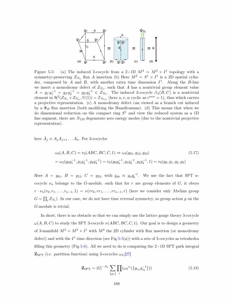
=
A
g2 g2'
g1 g1'
=
g1 g1'
g2 g2'
g3' g3
A
B C B
(a) (b) (c) A
A
= B
(d)
Figure 5-5: (a) The induced 2-cocycle from a 2+1D 𝑀3 = 𝑀2 × 𝐼1 topology with asymmetry-preserving 𝑍𝑁𝑢 flux 𝐴 insertion (b) Here 𝑀2 = 𝑆1 × 𝐼1 is a 2D spatial cylin-der, composed by 𝐴 and 𝐵, with another extra time dimension 𝐼1. Along the 𝐵-linewe insert a monodromy defect of 𝑍𝑁1 , such that 𝐴 has a nontrivial group element value𝐴 = 𝑔1′𝑔
−11 = 𝑔2′𝑔
−12 = 𝑔3′𝑔
−13 ∈ 𝑍𝑁1 . The induced 2-cocycle 𝛽𝐴(𝐵,𝐶) is a nontrivial
element in ℋ2(𝑍𝑁𝑣 ×𝑍𝑁𝑤 ,U(1)) = Z𝑁𝑣𝑤 (here 𝑢, 𝑣, 𝑤 cyclic as 𝜖𝑢𝑣𝑤 = 1), thus which carriesa projective representation. (c) A monodromy defect can viewed as a branch cut inducedby a Φ𝐵 flux insertion (both modifying the Hamiltonians). (d) This means that when wedo dimensional reduction on the compact ring 𝑆1 and view the reduced system as a 1Dline segment, there are 𝑁123 degenerate zero energy modes (due to the nontrivial projectiverepresentation).
here 𝐴𝑗 ≡ 𝐴𝑗𝐴𝑗+1 . . . 𝐴𝑛. For 3-cocycles
𝜔3(𝐴,𝐵,𝐶) = 𝜈3(𝐴𝐵𝐶,𝐵𝐶,𝐶, 1)⇒ 𝜔3(𝑔01, 𝑔12, 𝑔23) (5.17)
= 𝜔3(𝑔0𝑔−11 , 𝑔1𝑔
−12 , 𝑔2𝑔
−13 ) = 𝜈3(𝑔0𝑔
−13 , 𝑔1𝑔
−13 , 𝑔2𝑔
−13 , 1) = 𝜈3(𝑔0, 𝑔1, 𝑔2, 𝑔3)
Here 𝐴 = 𝑔01, 𝐵 = 𝑔12, 𝐶 = 𝑔23, with 𝑔𝑎𝑏 ≡ 𝑔𝑎𝑔−1𝑏 . We use the fact that SPT 𝑛-
cocycle 𝜈𝑛 belongs to the 𝐺-module, such that for 𝑟 are group elements of 𝐺, it obeys
𝑟 · 𝜈𝑛(𝑟0, 𝑟1, . . . , 𝑟𝑛−1, 1) = 𝜈(𝑟𝑟0, 𝑟𝑟1, . . . , 𝑟𝑟𝑛−1, 𝑟) (here we consider only Abelian group
𝐺 =∏𝑖 𝑍𝑁𝑖). In our case, we do not have time reversal symmetry, so group action 𝑔 on the
𝐺-module is trivial.
In short, there is no obstacle so that we can simply use the lattice gauge theory 3-cocycle
𝜔(𝐴,𝐵,𝐶) to study the SPT 3-cocycle 𝜈(𝐴𝐵𝐶,𝐵𝐶,𝐶, 1). Our goal is to design a geometry
of 3-manifold 𝑀3 = 𝑀2 × 𝐼1 with 𝑀2 the 2D cylinder with flux insertion (or monodromy
defect) and with the 𝐼1 time direction (see Fig.5-5(a)) with a sets of 3-cocycles as tetrahedra
filling this geometry (Fig.5-6). All we need to do is computing the 2+1D SPT path integral
ZSPT (i.e. partition function) using 3-cocycles 𝜔3,[27]
ZSPT = |𝐺|−𝑁𝑣∑{𝑔𝑣}
∏𝑖
(𝜔3𝑠𝑖({𝑔𝑣𝑎𝑔−1
𝑣𝑏})) (5.18)
168
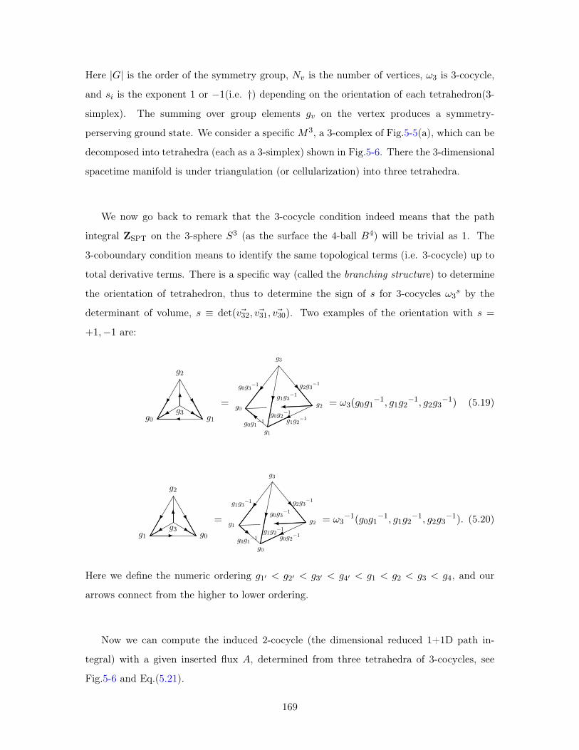
Here |𝐺| is the order of the symmetry group, 𝑁𝑣 is the number of vertices, 𝜔3 is 3-cocycle,
and 𝑠𝑖 is the exponent 1 or −1(i.e. †) depending on the orientation of each tetrahedron(3-
simplex). The summing over group elements 𝑔𝑣 on the vertex produces a symmetry-
perserving ground state. We consider a specific 𝑀3, a 3-complex of Fig.5-5(a), which can be
decomposed into tetrahedra (each as a 3-simplex) shown in Fig.5-6. There the 3-dimensional
spacetime manifold is under triangulation (or cellularization) into three tetrahedra.
We now go back to remark that the 3-cocycle condition indeed means that the path
integral ZSPT on the 3-sphere 𝑆3 (as the surface the 4-ball 𝐵4) will be trivial as 1. The
3-coboundary condition means to identify the same topological terms (i.e. 3-cocycle) up to
total derivative terms. There is a specific way (called the branching structure) to determine
the orientation of tetrahedron, thus to determine the sign of 𝑠 for 3-cocycles 𝜔3𝑠 by the
determinant of volume, 𝑠 ≡ det(𝑣32, 𝑣31, 𝑣30). Two examples of the orientation with 𝑠 =
+1,−1 are:
𝑔0 𝑔1𝑔3
𝑔2
= 𝑔0
𝑔1
𝑔2
𝑔3
𝑔0𝑔1−1 𝑔1𝑔2
−1
𝑔2𝑔3−1
𝑔0𝑔2−1
𝑔1𝑔3−1
𝑔0𝑔3−1
= 𝜔3(𝑔0𝑔1−1, 𝑔1𝑔2
−1, 𝑔2𝑔3−1) (5.19)
𝑔1 𝑔0𝑔3
𝑔2
= 𝑔1
𝑔0
𝑔2
𝑔3
𝑔0𝑔1−1 𝑔0𝑔2
−1
𝑔2𝑔3−1
𝑔1𝑔2−1
𝑔0𝑔3−1
𝑔1𝑔3−1
= 𝜔3−1(𝑔0𝑔1
−1, 𝑔1𝑔2−1, 𝑔2𝑔3
−1). (5.20)
Here we define the numeric ordering 𝑔1′ < 𝑔2′ < 𝑔3′ < 𝑔4′ < 𝑔1 < 𝑔2 < 𝑔3 < 𝑔4, and our
arrows connect from the higher to lower ordering.
Now we can compute the induced 2-cocycle (the dimensional reduced 1+1D path in-
tegral) with a given inserted flux 𝐴, determined from three tetrahedra of 3-cocycles, see
Fig.5-6 and Eq.(5.21).
169
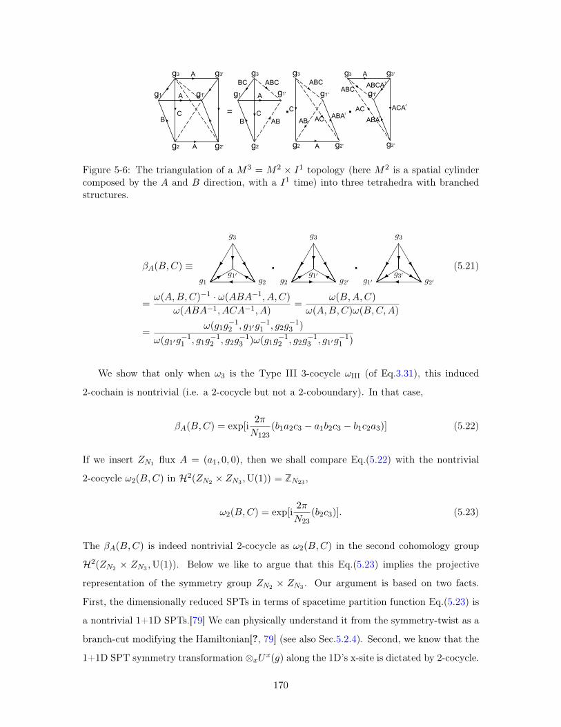
g1 g1'
g2 g2'
g3' g3
A
B C
A
A
g1 g1'
g2
g3
A
B
C
BC
AB
ABC
= . . g1'
g2'
g3' g3 A
AC
ABC
ACA -1
ABCA -1
ABA -1
g1'
g2 g2'
g3
AB
C
ABC
A
AC ABA -1
Figure 5-6: The triangulation of a 𝑀3 = 𝑀2 × 𝐼1 topology (here 𝑀2 is a spatial cylindercomposed by the 𝐴 and 𝐵 direction, with a 𝐼1 time) into three tetrahedra with branchedstructures.
𝛽𝐴(𝐵,𝐶) ≡𝑔1 𝑔2
𝑔1′
𝑔3
�
𝑔2 𝑔2′𝑔1′
𝑔3
�
𝑔1′ 𝑔2′𝑔3′
𝑔3
(5.21)
=𝜔(𝐴,𝐵,𝐶)−1 · 𝜔(𝐴𝐵𝐴−1, 𝐴,𝐶)
𝜔(𝐴𝐵𝐴−1, 𝐴𝐶𝐴−1, 𝐴)=
𝜔(𝐵,𝐴,𝐶)
𝜔(𝐴,𝐵,𝐶)𝜔(𝐵,𝐶,𝐴)
=𝜔(𝑔1𝑔
−12 , 𝑔1′𝑔
−11 , 𝑔2𝑔
−13 )
𝜔(𝑔1′𝑔−11 , 𝑔1𝑔
−12 , 𝑔2𝑔
−13 )𝜔(𝑔1𝑔
−12 , 𝑔2𝑔
−13 , 𝑔1′𝑔
−11 )
We show that only when 𝜔3 is the Type III 3-cocycle 𝜔III (of Eq.3.31), this induced
2-cochain is nontrivial (i.e. a 2-cocycle but not a 2-coboundary). In that case,
𝛽𝐴(𝐵,𝐶) = exp[i2𝜋
𝑁123(𝑏1𝑎2𝑐3 − 𝑎1𝑏2𝑐3 − 𝑏1𝑐2𝑎3)] (5.22)
If we insert 𝑍𝑁1 flux 𝐴 = (𝑎1, 0, 0), then we shall compare Eq.(5.22) with the nontrivial
2-cocycle 𝜔2(𝐵,𝐶) in ℋ2(𝑍𝑁2 × 𝑍𝑁3 ,U(1)) = Z𝑁23 ,
𝜔2(𝐵,𝐶) = exp[i2𝜋
𝑁23(𝑏2𝑐3)]. (5.23)
The 𝛽𝐴(𝐵,𝐶) is indeed nontrivial 2-cocycle as 𝜔2(𝐵,𝐶) in the second cohomology group
ℋ2(𝑍𝑁2 × 𝑍𝑁3 ,U(1)). Below we like to argue that this Eq.(5.23) implies the projective
representation of the symmetry group 𝑍𝑁2 × 𝑍𝑁3 . Our argument is based on two facts.
First, the dimensionally reduced SPTs in terms of spacetime partition function Eq.(5.23) is
a nontrivial 1+1D SPTs.[79] We can physically understand it from the symmetry-twist as a
branch-cut modifying the Hamiltonian[?, 79] (see also Sec.5.2.4). Second, we know that the
1+1D SPT symmetry transformation ⊗𝑥𝑈𝑥(𝑔) along the 1D’s x-site is dictated by 2-cocycle.
170
The onsite tensor 𝑆(𝑔) ≡ ⊗𝑥𝑈𝑥(𝑔) acts on a chain of 1D SPT renders
𝑆(𝑔)|𝛼𝐿, . . . , 𝛼𝑅⟩ =𝜔2(𝛼
−1𝐿 𝑔−1, 𝑔)
𝜔2(𝛼−1𝑅 𝑔−1, 𝑔)
|𝑔𝛼𝐿, . . . , 𝑔𝛼𝑅⟩, (5.24)
where 𝛼𝐿 and 𝛼𝑅 are the two ends of the chain, with 𝑔, 𝛼𝐿, 𝛼𝑅, · · · ∈ 𝐺 all in the symmetry
group. We can derive the effective degree of freedom on the 0D edge |𝛼𝐿⟩ forms a projective
representation of symmetry, we find:
𝑆(𝐵)𝑆(𝐶)|𝛼𝐿⟩ =𝜔2(𝛼
−1𝐿 𝐶−1𝐵−1, 𝐵)𝜔2(𝛼
−1𝐿 𝐶−1, 𝐵)
𝜔2(𝛼−1𝐿 𝐶−1𝐵−1, 𝐵𝐶)
𝑆(𝐵𝐶)|𝛼𝐿⟩ = 𝜔2(𝐵,𝐶)𝑆(𝐵𝐶)|𝛼𝐿⟩
(5.25)
In the last line, we implement the 2-cocycle condition of 𝜔2: 𝛿𝜔2(𝑎, 𝑏, 𝑐) =𝜔2(𝑏,𝑐)𝜔2(𝑎,𝑏𝑐)𝜔2(𝑎𝑏,𝑐)𝜔2(𝑎,𝑏)
= 1.
The projective representation of symmetry transformation 𝑆(𝐵)𝑆(𝐶) = 𝜔2(𝐵,𝐶)𝑆(𝐵𝐶) is
explicitly derived, and the projective phase is the 2-cocycle 𝜔2(𝐵,𝐶) classified byℋ2(𝐺,U(1)).
Interestingly, the symmetry transformations on two ends together will form a linear repre-
sentation, namely 𝑆(𝐵)𝑆(𝐶)|𝛼𝐿, . . . , 𝛼𝑅⟩ = 𝑆(𝐵𝐶)|𝛼𝐿, . . . , 𝛼𝑅⟩.
The same argument holds when 𝐴 is 𝑍𝑁2 flux or 𝑍𝑁3 flux. From Sec.5.2.2, the projective
representation of symmetry implies the nontrivial ground state degeneracy if we view the
system as a dimensionally-reduced 1D line segment as in Fig.5-5(d). From the 𝑁123 factor
in Eq.(5.22), we conclude there is 𝑁123-fold degenerated zero energy modes.
We should make two more remarks:
(i) The precise 1+1D path integral is actually summing over 𝑔𝑣 with a fixed flux 𝐴 as
ZSPT = |𝐺|−𝑁𝑣∑
{𝑔𝑣};fixed 𝐴 𝛽𝐴(𝐵,𝐶), but overall our discussion above still holds.
(ii) We have used 3-cocycle to construct a symmetry-preserving SPT ground state under
𝑍𝑁1 flux insertion. We can see that indeed a 𝑍𝑁1 symmetry-breaking domain wall of Fig.5-
7 can be done in almost the same calculation - using 3-cocycles filling a 2+1D spacetime
complex(Fig.5-7(a)). Although there in Fig.5-7(a), we need to fix the group elements 𝑔1 = 𝑔2
on one side (in the time independent domain wall profile, we need to fix 𝑔1 = 𝑔2 = 𝑔3) and/or
fix 𝑔′1 = 𝑔′2 on the other side. Remarkably, we conclude that both the 𝑍𝑁1-symmetry-
preserving flux insertion and 𝑍𝑁1 symmetry-breaking domain wall both provides
a 𝑁123-fold degenerate ground states (from the nontrivial projective representation for the
𝑍𝑁2 , 𝑍𝑁3 symmetry). The symmetry-breaking case is consitent with Sec.5.2.3.1.
171
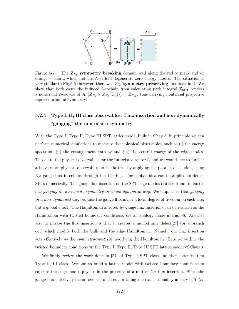
g2 g2'
g1
=
g1 g1'
g2 g2'
g3' g3
(a) (b)
x xx x
x
x
x x x
x
x x
+ + + + + +
+ + g1'
+ + + +
=
x xx xxx
+ + + + + +
(c)
Figure 5-7: The 𝑍𝑁1 symmetry breaking domain wall along the red × mark and/ororange + mark, which induces 𝑁123-fold degenerate zero energy modes. The situation isvery similar to Fig.5-5 (however, there was 𝑍𝑁1 symmetry-preserving flux insertion). Weshow that both cases the induced 2-cochain from calculating path integral ZSPT rendersa nontrivial 2-cocycle of ℋ2(𝑍𝑁2 × 𝑍𝑁3 ,U(1)) = Z𝑁23 , thus carrying nontrivial projectiverepresentation of symmetry.
5.2.4 Type I, II, III class observables: Flux insertion and non-dynamically
“gauging” the non-onsite symmetry
With the Type I, Type II, Type III SPT lattice model built in Chap.3, in principle we can
perform numerical simulations to measure their physical observables, such as (i) the energy
spectrum, (ii) the entanglement entropy and (iii) the central charge of the edge modes.
Those are the physical observables for the “untwisted sectors”, and we would like to further
achieve more physical observables on the lattice, by applying the parallel discussion, using
𝑍𝑁 gauge flux insertions through the 1D ring. The similar idea can be applied to detect
SPTs numerically. The gauge flux insertion on the SPT edge modes (lattice Hamiltonian) is
like gauging its non-onsite symmetry in a non-dynamical way. We emphasize that gauging
in a non-dynamical way because the gauge flux is not a local degree of freedom on each site,
but a global effect. The Hamiltonian affected by gauge flux insertions can be realized as the
Hamiltonian with twisted boundary conditions, see an analogy made in Fig.5-8. Another
way to phrase the flux insertion is that it creates a monodromy defect[27] (or a branch
cut) which modify both the bulk and the edge Hamiltonian. Namely, our flux insertion
acts effectively as the symmetry-twist [79] modifying the Hamiltonian. Here we outline the
twisted boundary conditions on the Type I, Type II, Type III SPT lattice model of Chap.3.
We firstly review the work done in [57] of Type I SPT class and then extends it to
Type II, III class. We aim to build a lattice model with twisted boundary conditions to
capture the edge modes physics in the presence of a unit of 𝑍𝑁 flux insertion. Since the
gauge flux effectively introduces a branch cut breaking the translational symmetry of 𝑇 (as
172
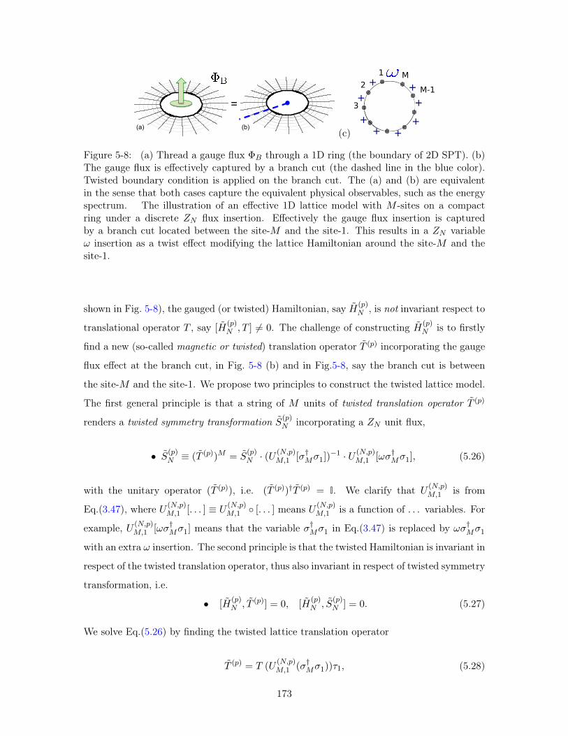
=
(a) (b) (c)
1
2M
M-1
3
-+
+
++ +
+
+
+
Figure 5-8: (a) Thread a gauge flux Φ𝐵 through a 1D ring (the boundary of 2D SPT). (b)The gauge flux is effectively captured by a branch cut (the dashed line in the blue color).Twisted boundary condition is applied on the branch cut. The (a) and (b) are equivalentin the sense that both cases capture the equivalent physical observables, such as the energyspectrum. The illustration of an effective 1D lattice model with 𝑀 -sites on a compactring under a discrete 𝑍𝑁 flux insertion. Effectively the gauge flux insertion is capturedby a branch cut located between the site-𝑀 and the site-1. This results in a 𝑍𝑁 variable𝜔 insertion as a twist effect modifying the lattice Hamiltonian around the site-𝑀 and thesite-1.
shown in Fig. 5-8), the gauged (or twisted) Hamiltonian, say ��(𝑝)𝑁 , is not invariant respect to
translational operator 𝑇 , say [��(𝑝)𝑁 , 𝑇 ] = 0. The challenge of constructing ��(𝑝)
𝑁 is to firstly
find a new (so-called magnetic or twisted) translation operator 𝑇 (𝑝) incorporating the gauge
flux effect at the branch cut, in Fig. 5-8 (b) and in Fig.5-8, say the branch cut is between
the site-𝑀 and the site-1. We propose two principles to construct the twisted lattice model.
The first general principle is that a string of 𝑀 units of twisted translation operator 𝑇 (𝑝)
renders a twisted symmetry transformation 𝑆(𝑝)𝑁 incorporating a 𝑍𝑁 unit flux,
∙ 𝑆(𝑝)𝑁 ≡ (𝑇 (𝑝))𝑀 = 𝑆
(𝑝)𝑁 · (𝑈
(𝑁,𝑝)𝑀,1 [𝜎†𝑀𝜎1])
−1 · 𝑈 (𝑁,𝑝)𝑀,1 [𝜔𝜎†𝑀𝜎1], (5.26)
with the unitary operator (𝑇 (𝑝)), i.e. (𝑇 (𝑝))†𝑇 (𝑝) = I. We clarify that 𝑈 (𝑁,𝑝)𝑀,1 is from
Eq.(3.47), where 𝑈 (𝑁,𝑝)𝑀,1 [. . . ] ≡ 𝑈 (𝑁,𝑝)
𝑀,1 ∘ [. . . ] means 𝑈 (𝑁,𝑝)𝑀,1 is a function of . . . variables. For
example, 𝑈 (𝑁,𝑝)𝑀,1 [𝜔𝜎†𝑀𝜎1] means that the variable 𝜎†𝑀𝜎1 in Eq.(3.47) is replaced by 𝜔𝜎†𝑀𝜎1
with an extra 𝜔 insertion. The second principle is that the twisted Hamiltonian is invariant in
respect of the twisted translation operator, thus also invariant in respect of twisted symmetry
transformation, i.e.
∙ [��(𝑝)𝑁 , 𝑇 (𝑝)] = 0, [��
(𝑝)𝑁 , 𝑆
(𝑝)𝑁 ] = 0. (5.27)
We solve Eq.(5.26) by finding the twisted lattice translation operator
𝑇 (𝑝) = 𝑇 (𝑈(𝑁,𝑝)𝑀,1 (𝜎†𝑀𝜎1))𝜏1, (5.28)
173
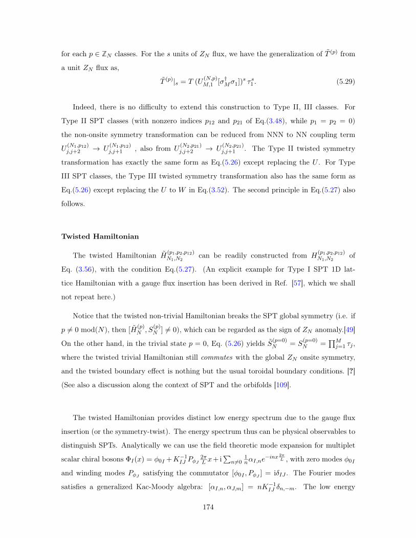
for each 𝑝 ∈ Z𝑁 classes. For the 𝑠 units of 𝑍𝑁 flux, we have the generalization of 𝑇 (𝑝) from
a unit 𝑍𝑁 flux as,
𝑇 (𝑝)|𝑠 = 𝑇 (𝑈(𝑁,𝑝)𝑀,1 [𝜎†𝑀𝜎1])
𝑠 𝜏 𝑠1 . (5.29)
Indeed, there is no difficulty to extend this construction to Type II, III classes. For
Type II SPT classes (with nonzero indices 𝑝12 and 𝑝21 of Eq.(3.48), while 𝑝1 = 𝑝2 = 0)
the non-onsite symmetry transformation can be reduced from NNN to NN coupling term
𝑈(𝑁1,𝑝12)𝑗,𝑗+2 → 𝑈
(𝑁1,𝑝12)𝑗,𝑗+1 , also from 𝑈
(𝑁2,𝑝21)𝑗,𝑗+2 → 𝑈
(𝑁2,𝑝21)𝑗,𝑗+1 . The Type II twisted symmetry
transformation has exactly the same form as Eq.(5.26) except replacing the 𝑈 . For Type
III SPT classes, the Type III twisted symmetry transformation also has the same form as
Eq.(5.26) except replacing the 𝑈 to 𝑊 in Eq.(3.52). The second principle in Eq.(5.27) also
follows.
Twisted Hamiltonian
The twisted Hamiltonian ��(𝑝1,𝑝2,𝑝12)𝑁1,𝑁2
can be readily constructed from 𝐻(𝑝1,𝑝2,𝑝12)𝑁1,𝑁2
of
Eq. (3.56), with the condition Eq.(5.27). (An explicit example for Type I SPT 1D lat-
tice Hamiltonian with a gauge flux insertion has been derived in Ref. [57], which we shall
not repeat here.)
Notice that the twisted non-trivial Hamiltonian breaks the SPT global symmetry (i.e. if
𝑝 = 0 mod(𝑁), then [��(𝑝)𝑁 , 𝑆
(𝑝)𝑁 ] = 0), which can be regarded as the sign of 𝑍𝑁 anomaly.[49]
On the other hand, in the trivial state 𝑝 = 0, Eq. (5.26) yields 𝑆(𝑝=0)𝑁 = 𝑆
(𝑝=0)𝑁 =
∏𝑀𝑗=1 𝜏𝑗 ,
where the twisted trivial Hamiltonian still commutes with the global 𝑍𝑁 onsite symmetry,
and the twisted boundary effect is nothing but the usual toroidal boundary conditions. [?]
(See also a discussion along the context of SPT and the orbifolds [109].
The twisted Hamiltonian provides distinct low energy spectrum due to the gauge flux
insertion (or the symmetry-twist). The energy spectrum thus can be physical observables to
distinguish SPTs. Analytically we can use the field theoretic mode expansion for multiplet
scalar chiral bosons Φ𝐼(𝑥) = 𝜑0𝐼 +𝐾−1𝐼𝐽 𝑃𝜑𝐽
2𝜋𝐿 𝑥+ i
∑��=0
1𝑛𝛼𝐼,𝑛𝑒
−𝑖𝑛𝑥 2𝜋𝐿 , with zero modes 𝜑0𝐼
and winding modes 𝑃𝜑𝐽 satisfying the commutator [𝜑0𝐼 , 𝑃𝜑𝐽 ] = i𝛿𝐼𝐽 . The Fourier modes
satisfies a generalized Kac-Moody algebra: [𝛼𝐼,𝑛, 𝛼𝐽,𝑚] = 𝑛𝐾−1𝐼𝐽 𝛿𝑛,−𝑚. The low energy
174
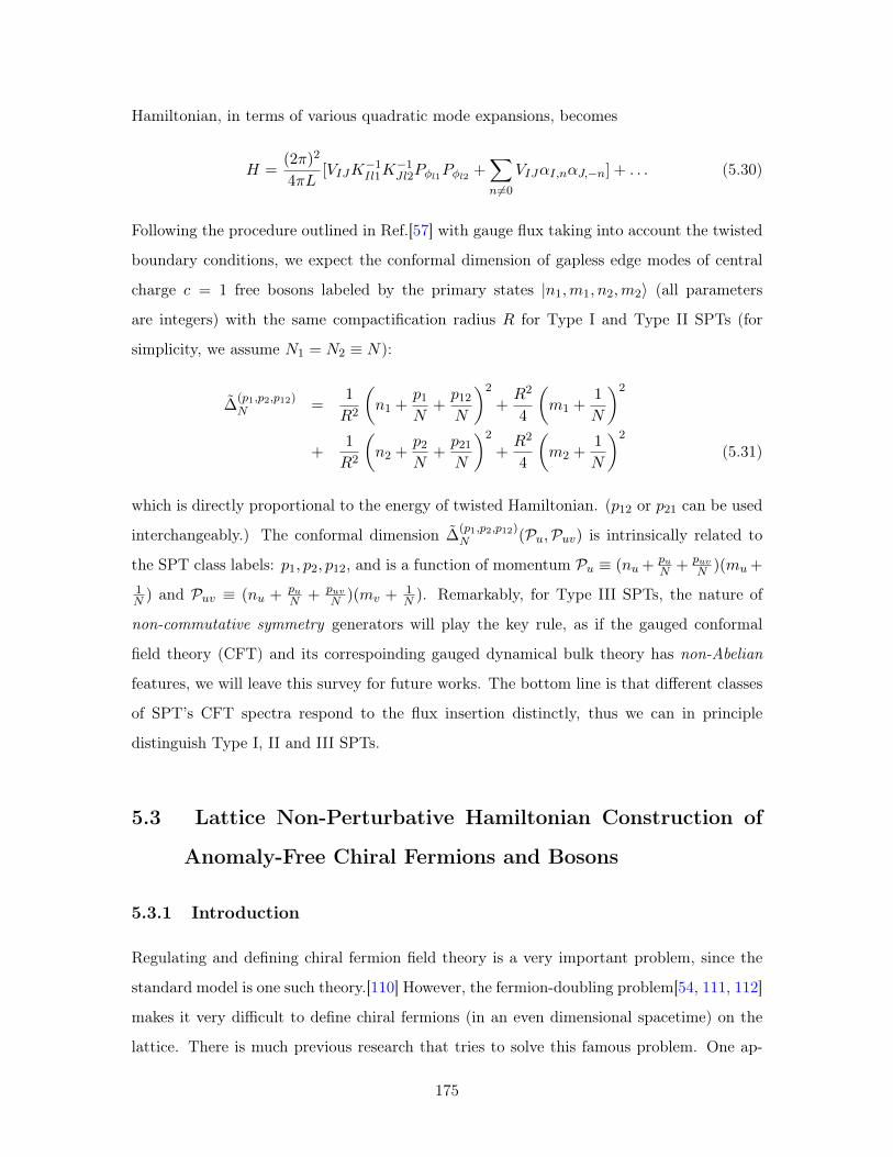
Hamiltonian, in terms of various quadratic mode expansions, becomes
𝐻 =(2𝜋)2
4𝜋𝐿[𝑉𝐼𝐽𝐾
−1𝐼𝑙1𝐾
−1𝐽𝑙2𝑃𝜑𝑙1𝑃𝜑𝑙2 +
∑��=0
𝑉𝐼𝐽𝛼𝐼,𝑛𝛼𝐽,−𝑛] + . . . (5.30)
Following the procedure outlined in Ref.[57] with gauge flux taking into account the twisted
boundary conditions, we expect the conformal dimension of gapless edge modes of central
charge 𝑐 = 1 free bosons labeled by the primary states |𝑛1,𝑚1, 𝑛2,𝑚2⟩ (all parameters
are integers) with the same compactification radius 𝑅 for Type I and Type II SPTs (for
simplicity, we assume 𝑁1 = 𝑁2 ≡ 𝑁):
Δ(𝑝1,𝑝2,𝑝12)𝑁 =
1
𝑅2
(𝑛1 +
𝑝1𝑁
+𝑝12𝑁
)2
+𝑅2
4
(𝑚1 +
1
𝑁
)2
+1
𝑅2
(𝑛2 +
𝑝2𝑁
+𝑝21𝑁
)2
+𝑅2
4
(𝑚2 +
1
𝑁
)2
(5.31)
which is directly proportional to the energy of twisted Hamiltonian. (𝑝12 or 𝑝21 can be used
interchangeably.) The conformal dimension Δ(𝑝1,𝑝2,𝑝12)𝑁 (𝒫𝑢,𝒫𝑢𝑣) is intrinsically related to
the SPT class labels: 𝑝1, 𝑝2, 𝑝12, and is a function of momentum 𝒫𝑢 ≡ (𝑛𝑢+𝑝𝑢𝑁 + 𝑝𝑢𝑣
𝑁 )(𝑚𝑢+
1𝑁 ) and 𝒫𝑢𝑣 ≡ (𝑛𝑢 + 𝑝𝑢
𝑁 + 𝑝𝑢𝑣𝑁 )(𝑚𝑣 +
1𝑁 ). Remarkably, for Type III SPTs, the nature of
non-commutative symmetry generators will play the key rule, as if the gauged conformal
field theory (CFT) and its correspoinding gauged dynamical bulk theory has non-Abelian
features, we will leave this survey for future works. The bottom line is that different classes
of SPT’s CFT spectra respond to the flux insertion distinctly, thus we can in principle
distinguish Type I, II and III SPTs.
5.3 Lattice Non-Perturbative Hamiltonian Construction of
Anomaly-Free Chiral Fermions and Bosons
5.3.1 Introduction
Regulating and defining chiral fermion field theory is a very important problem, since the
standard model is one such theory.[110] However, the fermion-doubling problem[54, 111, 112]
makes it very difficult to define chiral fermions (in an even dimensional spacetime) on the
lattice. There is much previous research that tries to solve this famous problem. One ap-
175
proach is the lattice gauge theory,[113] which is unsuccessful since it cannot reproduce chiral
couplings between the gauge fields and the fermions. Another approach is the domain-wall
fermion.[114, 115] However, the gauge field in the domain-wall fermion approach propa-
gates in one-higher dimension. Another approach is the overlap-fermion,[116, 117] while
the path-integral in the overlap-fermion approach may not describe a finite quantum the-
ory with a finite Hilbert space for a finite space-lattice. There is also the mirror fermion
approach[118, 119, 120, 121] which starts with a lattice model containing chiral fermions in
one original light sector coupled to gauge theory, and its chiral conjugated as the mirror
sector. Then, one tries to include direct interactions or boson mediated interactions[122]
between fermions to gap out the mirror sector only. However, the later works either fail to
demonstrate [123, 124, 125] or argue that it is almost impossible to gap out (i.e. fully open
the mass gaps of) the mirror sector without breaking the gauge symmetry in some mirror
fermion models.[126]
We realized that the previous failed lattice-gauge approaches always assume non-interacting
lattice fermions (apart from the interaction to the lattice gauge field). In this work, we show
that lattice approach actually works if we include direct fermion-fermion interaction with
appropriate strength (i.e. the dimensionaless coupling constants are of order 1).[49, 127] In
other words, a general framework of the mirror fermion approach actually works for con-
structing a lattice chiral fermion theory, at least in 1+1D. Specifically, any anomaly-free
chiral fermion/boson field theory can be defined as a finite quantum system on a 1D lattice
where the (gauge or global) symmetry is realized as an onsite symmetry, provided that we
allow lattice fermion/boson to have interactions, instead of being free. (Here, the “chiral”
theory here means that it “breaks parity 𝑃 symmetry.” Our 1+1D chiral fermion theory
breaks parity 𝑃 and time reversal 𝑇 symmetry. Our insight comes from Ref. [49, 127], where
the connection between gauge anomalies and symmetry-protected topological (SPT) states
(in one-higher dimension) is found.
To make our readers fully appreciate our thinking, we shall firstly define our important
basic notions clearly:
(◇1) Onsite symmetry means that the overall symmetry transformation 𝑈(𝑔) of symmetry
group 𝐺 can be defined as the tensor product of each single site’s symmetry transformation
𝑈𝑖(𝑔), via 𝑈(𝑔) = ⊗𝑖𝑈𝑖(𝑔) with 𝑔 ∈ 𝐺. Nonsite symmetry : means 𝑈(𝑔)non-onsite = ⊗𝑖𝑈𝑖(𝑔).
176
(◇2) Local Hamiltonian with short-range interactions means that the non-zero amplitude of
matter(fermion/boson) hopping/interactions in finite time has a finite range propagation,
and cannot be an infinite range. Strictly speaking, the quasi-local exponential decay (of
kinetic hopping/interactions) is non-local and not short-ranged.
(◇3) finite(-Hilbert-space) system means that the dimension of Hilbert space is finite if the
system has finite lattice sites (e.g. on a cylinder).
Nielsen-Ninomiya theorem[54, 111, 112] states that the attempt to regularize chiral
fermion on a lattice as a local free non-interacting fermion model with fermion number
conservation (i.e. with U(1) symmetry) has fermion-doubling problem[54, 111, 112] in an
even dimensional spacetime. To apply this no-go theorem, however, the symmetry is as-
sumed to be an onsite symmetry.
Ginsparg-Wilson fermion approach copes with this no-go theorem by solving Ginsparg-
Wilson(GW) relation[70, 71] based on the quasi-local Neuberger-Dirac operator,[72, 73, 74]
where quasi-local is strictly non-local. In this work, we show that the quasi-localness of
Neuberger-Dirac operator in the GW fermion approach imposing a non-onsite[97, 57] U(1)
symmetry, instead of an onsite symmetry. (While here we simply summarize the result, one
can read the details of onsite and non-onsite symmetry, and its relation to GW fermion in
[50].) For our specific approach for the mirror-fermion decoupling, we will not implement the
GW fermions (of non-onsite symmetry) construction, instead, we will use a lattice fermions
with onsite symmetry but with particular properly-designed interactions. Comparing GW
fermion to our approach, we see that
• Ginsparg-Wilson(GW) fermion approach obtains “chiral fermions from a local
free fermion lattice model with non-onsite U(1) symmetry (without fermion doublers).”
(Here one regards Ginsparg-Wilson fermion applying the Neuberger-Dirac operator,
which is strictly non-onsite and non-local.)
• Our approach obtains “chiral fermions from local interacting fermion lattice model
with onsite 𝑈(1) symmetry (without fermion doublers), if all U(1) anomalies are can-
ncelled.”
Also, the conventional GW fermion approach discretizes the Lagrangian/the action on
the spacetime lattice, while we use a local short-range quantum Hamiltonian on 1D spatial
lattice with a continuous time. Such a distinction causes some difference. For example, it is
177
known that Ginsparg-Wilson fermion can implement a single Weyl fermion for the free case
without gauge field on a 1+1D space-time-lattice due to the works of Neuberger, Lüscher,
etc. Our approach cannot implement a single Weyl fermion on a 1D space-lattice within
local short-range Hamiltonian. (However, such a distinction may not be important if we are
allowed to introduce a non-local infinite-range hopping.)
Comparison to Eichten-Preskill and Chen-Giedt-Poppitz models: Due to the past
investigations, a majority of the high-energy lattice community believes that the mirror-
fermion decoupling (or lattice gauge approach) fails to realize chiral fermion or chiral gauge
theory. Thus one may challenge us by asking “how our mirror-fermion decoupling model
is different from Eichten-Preskill and Chen-Giedt-Poppitz models?” And “why the recent
numerical attempt of Chen-Giedt-Poppitz fails?[125]” We now stress that, our approach
provides properly designed fermion interaction terms to make things work, due to the recent
understanding to topological gapped boundary conditions[60, 68]:
• Eichten-Preskill(EP)[118] propose a generic idea of the mirror-fermion approach
for the chiral gauge theory. There the perturbative analysis on the weak-coupling and
strong-coupling expansions are used to demonstrate possible mirror-fermion decoupling
phase can exist in the phase diagram. The action is discretized on the spacetime
lattice. In EP approach, one tries to gap out the mirror-fermions via the mass term
of composite fermions that do not break the (gauge) symmetry on lattice. The mass
term of composite fermions are actually fermion interacting terms. So in EP approach,
one tries to gap out the mirror-fermions via the direct fermion interaction that do not
break the (gauge) symmetry on lattice. However, considering only the symmetry of
the interaction is not enough. Even when the mirror sector is anomalous, one can still
add the direct fermion interaction that do not break the (gauge) symmetry. So the
presence of symmetric direct fermion interaction may or may not be able to gap out
the mirror sector. When the mirror sector is anomaly-free, we will show in this paper,
some symmetric interactions are helpful for gapping out the mirror sectors, while other
symmetric interactions are harmful. The key issue is to design the proper interaction
to gap out the mirror section, and considering only symmetry is not enough.
• Chen-Giedt-Poppitz(CGP)[125] follows the EP general framework to deal with
178
a 3-4-5 anomaly-free model with a single U(1) symmetry. All the U(1) symmetry-
allowed Yukawa-Higgs terms are introduced to mediate multi-fermion interactions.
The Ginsparg-Wilson fermion and the Neuberger’s overlap Dirac operator are im-
plemented, the fermion actions are discretized on the spacetime lattice. Again, the
interaction terms are designed only based on symmetry, which contain both helpful
and harmful terms, as we will show.
• Our model in general belongs to the mirror-fermion-decoupling idea. The anomaly-
free model we proposed is named as the 3𝐿-5𝑅-4𝐿-0𝑅 model. Our 3𝐿-5𝑅-4𝐿-0𝑅 is
in-reality different from Chen-Giedt-Poppitz’s 3-4-5 model, since we impliment:
(i) an onsite-symmetry local lattice model: Our lattice Hamiltonian is built on
1D spatial lattice with on-site U(1) symmetry. We neither implement the GW fermion
nor the Neuberger-Dirac operator (both have non-onsite symmetry).
(ii) a particular set of interaction terms with proper strength:
Our multi fermion interaction terms are particularly-designed gapping terms which
obey not only the symmetry but also certain Lagrangian subgroup algebra. Those
interaction terms are called helpful gapping terms, satisfying Boundary Fully Gap-
ping Rules. We will show that the Chen-Giedt-Poppitz’s Yukawa-Higgs terms induce
extra multi-fermion interaction terms which do not satsify Boundary Fully Gap-
ping Rules. Those extra terms are incompatible harmful terms, competing with the
helpful gapping terms and causing the preformed mass gap unstable so preventing the
mirror sector from being gapped out. (This can be one of the reasons for the failure of
mirror-decoupling in Ref.[125].) We stress that, due to a topological non-perturbative
reason, only a particular set of ideal interaction terms are helpful to fully gap the
mirror sector. Adding more or removing interactions can cause the mass gap unstable
thus the phase flowing to gapless states. In addition, we stress that only when the
helpful interaction terms are in a proper range, intermediate strength for dimensionless
coupling of order 1, can they fully gap the mirror sector, and yet not gap the original
sector (details in Sec.5.3.4). Throughout our work, when we say strong coupling for
our model, we really mean intermediate(-strong) coupling in an appropriate range. In
CGP model, however, their strong coupling may be too strong (with their kinetic term
neglected); which can be another reason for the failure of mirror-decoupling.[125]
179
(iii) extra symmetries: For our model, a total even number 𝑁 of left/right moving
Weyl fermions (𝑁𝐿 = 𝑁𝑅 = 𝑁/2), we will add only 𝑁/2 helpful gapping terms under
the constraint of the Lagrangian subgroup algebra and Boundary Fully Gapping
Rules. As a result, the full symmetry of our lattice model is U(1)𝑁/2 (where the gap-
ping terms break U(1)𝑁 down to U(1)𝑁/2). For the case of our 3𝐿-5𝑅-4𝐿-0𝑅 model, the
full U(1)2 symmetry has two sets of U(1) charges, U(1)1st 3-5-4-0 and U(1)2nd 0-4-5-3,
both are anomaly-free and mixed-anomaly-free. Although the physical consideration
only requires the interaction terms to have on-site U(1)1st symmetry, looking for in-
teraction terms with extra U(1) symmetry can help us to identify the helpful gapping
terms and design the proper lattice interactions. CGP model has only a single U(1)1st
symmetry. Here we suggest to improve that model by removing all the interaction
terms that break the U(1)2nd symmetry (thus adding all possible terms that preserve
the two U(1) symmetries) with an intermediate strength.
The plan of our attack is the following. In Sec.5.3.2 we first consider a 3𝐿-5𝑅-4𝐿-0𝑅
anomaly-free chiral fermion field theory model, with a full U(1)2 symmetry: A first 3-5-
4-0 U(1)1st symmetry for two left-moving fermions of charge-3 and charge-4, and for two
right-moving fermions of charge-5 and charge-0. And a second 0-4-5-3 U(1)2nd symmetry
for two left-moving fermions of charge-0 and charge-5, and for two right-moving fermions of
charge-4 and charge-3. If we wish to have a single U(1)1st symmetry, we can weakly break
the U(1)2nd symmetry by adding tiny local U(1)2nd-symmetry breaking term.
We claim that this model can be put on the lattice with an onsite U(1) symmetry, but
without fermion-doubling problem. We construct a 2+1D lattice model by simply using four
layers of the zeroth Landau levels(or more precisely, four filled bands with Chern numbers
[128] −1,+1,−1,+1 on a lattice) right-moving, charge-4 left-moving, charge-0 right-moving,
totally four fermionic modes at low energy on one edge. Therefore, by putting the 2D bulk
spatial lattice on a cylinder with two edges, one can leave edge states on one edge untouched
so they remain chiral and gapless, while turning on interactions to gap out the mirrored
edge states on the other edge with a large mass gap.
[NOTE on usages: Here in our work, U(1) symmetry may generically imply copies of U(1)
symmetry such as U(1)𝑀 , with positive integer 𝑀 . (Topological) Boundary Fully Gap-
ping Rules are defined as the rules to open the mass gaps of the boundary states. (Topolog-
ical) Gapped Boundary Conditions are defined to specify certain boundary types which
180
are gapped (thus topological). There are two kinds of usages of lattices here discussed in our
work: one is the Hamiltonian lattice model to simulate the chiral fermions/bosons. The
other lattice is the Chern-Simons lattice structure of Hilbert space, which is a quantized
lattice due to the level/charge quantization of Chern-Simons theory. ]
5.3.2 3𝐿-5𝑅-4𝐿-0𝑅 Chiral Fermion model
The simplest chiral (Weyl) fermion field theory with U(1) symmetry in 1 + 1D is given by
the action
𝑆Ψ,𝑓𝑟𝑒𝑒 =
∫𝑑𝑡𝑑𝑥 i𝜓†
𝐿(𝜕𝑡 − 𝜕𝑥)𝜓𝐿. (5.32)
However, Nielsen-Ninomiya theorem claims that such a theory cannot be put on a lattice
with unbroken onsite U(1) symmetry, due to the fermion-doubling problem.[54, 111, 112]
While the Ginsparg-Wilson fermion approach can still implement an anomalous single Weyl
fermion on the lattice, our approach cannot (unless we modify local Hamiltonian to infinite-
range hopping non-local Hamiltonian). As we will show, our approach is more restricted,
only limited to the anomaly-free theory. Let us instead consider an anomaly-free 3𝐿-5𝑅-4𝐿-
0𝑅 chiral fermion field theory with an action 𝑆ΨA,𝑓𝑟𝑒𝑒,∫𝑑𝑡𝑑𝑥
(i𝜓†𝐿,3(𝜕𝑡− 𝜕𝑥)𝜓𝐿,3 + i𝜓†
𝑅,5(𝜕𝑡+ 𝜕𝑥)𝜓𝑅,5 + i𝜓†𝐿,4(𝜕𝑡− 𝜕𝑥)𝜓𝐿,4 + i𝜓†
𝑅,0(𝜕𝑡+ 𝜕𝑥)𝜓𝑅,0
),
(5.33)
where 𝜓𝐿,3, 𝜓𝑅,5, 𝜓𝐿,4, and 𝜓𝑅,0 are 1-component Weyl spinor, carrying U(1) charges 3,5,4,0
respectively. The subscript 𝐿(or 𝑅) indicates left(or right) moving along −��(or +��). Al-
though this theory has equal numbers of left and right moving modes, it violates parity and
time reversal symmetry, so it is a chiral theory. Such a chiral fermion field theory is very
special because it is free from U(1) anomaly - it satisfies the anomaly matching condition[48]
in 1 + 1D, which means∑
𝑗 𝑞2𝐿,𝑗 − 𝑞2𝑅,𝑗 = 32 − 52 + 42 − 02 = 0. We ask:
Question 1: “Whether there is a local finite Hamiltonian realizing the above U(1) 3-5-4-0
symmetry as an onsite symmetry with short-range interactions defined on a 1D spatial
lattice with a continuous time, such that its low energy physics produces the anomaly-free
chiral fermion theory Eq.(5.33)?”
Yes. We would like to show that the above chiral fermion field theory can be put on
a lattice with unbroken onsite U(1) symmetry, if we include properly-desgined interactions
181
between fermions. In fact, we propose that the chiral fermion field theory in Eq.(5.33)
appears as the low energy effective theory of the following 2+1D lattice model on a cylinder
(see Fig.5-9) with a properly designed Hamiltonian. To derive such a Hamiltonian, we start
from thinking the full two-edges fermion theory with the action 𝑆Ψ, where the particularly
chosen multi-fermion interactions 𝑆ΨB,𝑖𝑛𝑡𝑒𝑟𝑎𝑐𝑡 will be explained:
𝑆Ψ = 𝑆ΨA,𝑓𝑟𝑒𝑒 + 𝑆ΨB,𝑓𝑟𝑒𝑒 + 𝑆ΨB,𝑖𝑛𝑡𝑒𝑟𝑎𝑐𝑡 =
∫𝑑𝑡 𝑑𝑥
(iΨAΓ
𝜇𝜕𝜇ΨA + iΨBΓ𝜇𝜕𝜇ΨB
+𝑔1((𝜓𝑅,3)(𝜓𝐿,5)(𝜓
†𝑅,4∇𝑥𝜓
†𝑅,4)(𝜓𝑅,0∇𝑥𝜓𝑅,0) + h.c.
)+𝑔2
((𝜓𝐿,3∇𝑥𝜓𝐿,3)(𝜓†
𝑅,5∇𝑥𝜓†𝑅,5)(𝜓𝐿,4)(𝜓𝐿,0) + h.c.
)), (5.34)
The notation for fermion fields on the edge A are ΨA = (𝜓𝐿,3, 𝜓𝑅,5, 𝜓𝐿,4, 𝜓𝑅,0) , and
fermion fields on the edge B are ΨB = (𝜓𝐿,5, 𝜓𝑅,3, 𝜓𝐿,0, 𝜓𝑅,4). (Here a left moving mode in
ΨA corresponds to a right moving mode in ΨB because of Landau level/Chern band chirality,
the details of lattice model will be explained.) The gamma matrices in 1+1D are presented
in terms of Pauli matrices, with 𝛾0 = 𝜎𝑥, 𝛾1 = i𝜎𝑦, 𝛾5 ≡ 𝛾0𝛾1 = −𝜎𝑧, and Γ0 = 𝛾0 ⊕ 𝛾0,
Γ1 = 𝛾1 ⊕ 𝛾1, Γ5 ≡ Γ0Γ1 and Ψ𝑖 ≡ Ψ𝑖Γ0.
In 1+1D, we can do bosonization, where the fermion matter field Ψ turns into bosonic
phase field Φ, more explicitly 𝜓𝐿,3 ∼ 𝑒iΦA3 , 𝜓𝑅,5 ∼ 𝑒iΦ
A5 , 𝜓𝐿,4 ∼ 𝑒iΦ
A4 , 𝜓𝑅,0 ∼ 𝑒iΦ
A0 on A edge,
𝜓𝑅,3 ∼ 𝑒iΦB3 , 𝜓𝐿,5 ∼ 𝑒iΦ
B5 , 𝜓𝑅,4 ∼ 𝑒iΦ
B4 , 𝜓𝐿,0 ∼ 𝑒iΦ
B0 on B edge, up to normal orderings : 𝑒iΦ :
and prefactors,[?] but the precise factor is not of our interest since our goal is to obtain its
non-perturbative lattice realization. So Eq.(5.34) becomes
𝑆Φ = 𝑆ΦA𝑓𝑟𝑒𝑒
+ 𝑆ΦB𝑓𝑟𝑒𝑒
+ 𝑆ΦB𝑖𝑛𝑡𝑒𝑟𝑎𝑐𝑡
=
1
4𝜋
∫𝑑𝑡𝑑𝑥
(𝐾A𝐼𝐽𝜕𝑡Φ
A𝐼 𝜕𝑥Φ
A𝐽 − 𝑉𝐼𝐽𝜕𝑥ΦA
𝐼 𝜕𝑥ΦA𝐽
)+(𝐾B𝐼𝐽𝜕𝑡Φ
B𝐼 𝜕𝑥Φ
B𝐽 − 𝑉𝐼𝐽𝜕𝑥ΦB
𝐼 𝜕𝑥ΦB𝐽
)+
∫𝑑𝑡𝑑𝑥
(𝑔1 cos(ΦB
3 +ΦB5 − 2ΦB
4 + 2ΦB0 ) + 𝑔2 cos(2ΦB
5 − 2ΦB5 +ΦB
4 +ΦB0 )
). (5.35)
Here 𝐼, 𝐽 runs over 3, 5, 4, 0 and 𝐾A𝐼𝐽 = −𝐾B
𝐼𝐽 = diag(1,−1, 1,−1) 𝑉𝐼𝐽 = diag(1, 1, 1, 1)
are diagonal matrices. All we have to prove is that gapping terms, the cosine terms
with 𝑔1, 𝑔2 coupling can gap out all states on the edge B. First, let us understand more
about the full U(1) symmetry. What are the U(1) symmetries? They are transformations
182
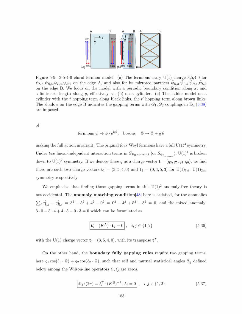
L3 L4
R5 R0
L5 L0
R3 R4 (a) (c)
A AB B
x
y L3 L4
R5
L5 L0
R3 R4 R0 (b)
A B
x
y
Figure 5-9: 3-5-4-0 chiral fermion model: (a) The fermions carry U(1) charge 3,5,4,0 for𝜓𝐿,3,𝜓𝑅,5,𝜓𝐿,4,𝜓𝑅,0 on the edge A, and also for its mirrored partners 𝜓𝑅,3,𝜓𝐿,5,𝜓𝑅,4,𝜓𝐿,0on the edge B. We focus on the model with a periodic boundary condition along 𝑥, anda finite-size length along 𝑦, effectively as, (b) on a cylinder. (c) The ladder model on acylinder with the 𝑡 hopping term along black links, the 𝑡′ hopping term along brown links.The shadow on the edge B indicates the gapping terms with 𝐺1, 𝐺2 couplings in Eq.(5.38)are imposed.
of
fermions 𝜓 → 𝜓 · 𝑒i𝑞𝜃, bosons Φ→ Φ+ 𝑞 𝜃
making the full action invariant. The original four Weyl fermions have a full U(1)4 symmetry.
Under two linear-indepndent interaction terms in 𝑆ΨB,𝑖𝑛𝑡𝑒𝑟𝑎𝑐𝑡 (or 𝑆ΦB𝑖𝑛𝑡𝑒𝑟𝑎𝑐𝑡
), U(1)4 is broken
down to U(1)2 symmetry. If we denote these 𝑞 as a charge vector t = (𝑞3, 𝑞5, 𝑞4, 𝑞0), we find
there are such two charge vectors t1 = (3, 5, 4, 0) and t2 = (0, 4, 5, 3) for U(1)1st, U(1)2nd
symmetry respectively.
We emphasize that finding those gapping terms in this U(1)2 anomaly-free theory is
not accidental. The anomaly matching condition[48] here is satisfied, for the anomalies∑𝑗 𝑞
2𝐿,𝑗 − 𝑞2𝑅,𝑗 = 32 − 52 + 42 − 02 = 02 − 42 + 52 − 32 = 0, and the mixed anomaly:
3 · 0− 5 · 4 + 4 · 5− 0 · 3 = 0 which can be formulated as
t𝑇𝑖 · (𝐾A) · t𝑗 = 0 , 𝑖, 𝑗 ∈ {1, 2} (5.36)
with the U(1) charge vector t = (3, 5, 4, 0), with its transpose t𝑇 .
On the other hand, the boundary fully gapping rules require two gapping terms,
here 𝑔1 cos(ℓ1 · Φ) + 𝑔2 cos(ℓ2 · Φ), such that self and mutual statistical angles 𝜃𝑖𝑗 defined
below among the Wilson-line operators ℓ𝑖, ℓ𝑗 are zeros,
𝜃𝑖𝑗/(2𝜋) ≡ ℓ𝑇𝑖 · (𝐾B)−1 · ℓ𝑗 = 0 , 𝑖, 𝑗 ∈ {1, 2} (5.37)
183
Indeed, here we have ℓ1 = (1, 1,−2, 2), ℓ2 = (2,−2, 1, 1) satisfying the rules. Thus we prove
that the mirrored edge states on the edge B can be fully gapped out.
We will prove the anomaly matching condition is equivalent to find a set of gapping
terms 𝑔𝑎 cos(ℓ𝑎·Φ), satisfies the boundary fully gapping rules, detailed in Sec.5.3.7, 5.3.8.
Simply speaking, the anomaly matching condition (Eq.(5.36)) in 1+1D is equivalent
to (an if and only if relation) the boundary fully gapping rules (Eq.(5.37)) in 1+1D
boundary/2+1D bulk for an equal number of left-right moving modes(𝑁𝐿 = 𝑁𝑅, with
central charge 𝑐𝐿 = 𝑐𝑅). We prove this is true at least for U(1) symmetry case, with the
bulk theory is a 2+1D SPT state and the boundary theory is in 1+1D.
We now propose a lattice Hamiltonian model for this 3𝐿-5𝑅-4𝐿-0𝑅 chiral
fermion realizing Eq.(5.34) (thus Eq.(5.33) at the low energy once the Edge B is gapped
out). Importantly, we do not discretize the action Eq.(5.34) on the spacetime lattice. We
do not use Ginsparg-Wilson(GW) fermion nor the Neuberger-Dirac operator. GW and
Neuberger-Dirac scheme contains non-onsite symmetry which cause the lattice difficult to
be gauged to chiral gauge theory. Instead, the key step is that we implement the on-site
symmetry lattice fermion model. The free kinetic part is a fermion-hopping model which
has a finite 2D bulk energy gap but with gapless 1D edge states. This can be done by using
any lattice Chern insulator.
We stress that any lattice Chern insulator with onsite-symmetry shall work, and we
design one as in Fig.5-9. Our full Hamiltonian with two interacting 𝐺1, 𝐺2 gapping terms is
𝐻 =∑
𝑞=3,5,4,0
(∑⟨𝑖,𝑗⟩
(𝑡𝑖𝑗,𝑞 𝑓
†𝑞 (𝑖)𝑓𝑞(𝑗) + ℎ.𝑐.
)+
∑⟨⟨𝑖,𝑗⟩⟩
(𝑡′𝑖𝑗,𝑞 𝑓
†𝑞 (𝑖)𝑓𝑞(𝑗) + ℎ.𝑐.
))(5.38)
+ 𝐺1
∑𝑗∈B
((𝑓3(𝑗)
)1(𝑓5(𝑗)
)1(𝑓 †4(𝑗)𝑝𝑡.𝑠.
)2(𝑓0(𝑗)𝑝𝑡.𝑠.
)2+ ℎ.𝑐.
)
+𝐺2
∑𝑗∈B
((𝑓3(𝑗)𝑝𝑡.𝑠.
)2(𝑓 †5(𝑗)𝑝𝑡.𝑠.
)2(𝑓4(𝑗)
)1(𝑓0(𝑗)
)1+ ℎ.𝑐.
)
where∑
𝑗∈B sums over the lattice points on the right boundary (the edge B in Fig.5-
9), and the fermion operators 𝑓3, 𝑓5, 𝑓4, 𝑓0 carry a U(1)1st charge 3,5,4,0 and another
U(1)2nd charge 0,4,5,3 respectively. We emphasize that this lattice model has onsite U(1)2
symmetry, since this Hamiltonian, including interaction terms, is invariant under a global
U(1)1st transformation on each site for any 𝜃 angle: 𝑓3 → 𝑓3𝑒i3𝜃, 𝑓5 → 𝑓5𝑒
i5𝜃, 𝑓4 → 𝑓4𝑒i4𝜃,
184
𝑓0 → 𝑓0, and invariant under another global U(1)2nd transformation for any 𝜃 angle: 𝑓3 → 𝑓3,
𝑓5 → 𝑓5𝑒i4𝜃, 𝑓4 → 𝑓4𝑒
i5𝜃, 𝑓0 → 𝑓0𝑒i3𝜃. The U(1)1st charge is the reason why it is named as
3𝐿-5𝑅-4𝐿-0𝑅 model.
As for notations, ⟨𝑖, 𝑗⟩ stands for nearest-neighbor hopping along black links and ⟨⟨𝑖, 𝑗⟩⟩
stands for next-nearest-neighbor hopping along brown links in Fig.5-9. Here 𝑝𝑡.𝑠. stands
for point-splitting. For example, (𝑓3(𝑗)𝑝𝑡.𝑠.)2 ≡ 𝑓3(𝑗)𝑓3(𝑗 + ��). We stress that the full
Hamiltonian (including interactions) Eq.(5.38) is short-ranged and local, because each term
only involves coupling within finite number of neighbor sites. The hopping amplitudes 𝑡𝑖𝑗,3 =
𝑡𝑖𝑗,4 and 𝑡′𝑖𝑗,3 = 𝑡′𝑖𝑗,4 produce bands with Chern number −1, while the hopping amplitudes
𝑡𝑖𝑗,5 = 𝑡𝑖𝑗,0 and 𝑡′𝑖𝑗,5 = 𝑡′𝑖𝑗,0 produce bands with Chern number +1 (see Sec.5.3.3.3).[128] The
ground state is obtained by filling the above four bands.
As Eq.(5.38) contains U(1)1st and an accidental extra U(1)2nd symmetry, we shall ask:
Question 2: “Whether there is a local finite Hamiltonian realizing only a U(1) 3-5-
4-0 symmetry as an onsite symmetry with short-range interactions defined on a 1D
spatial lattice with a continuous time, such that its low energy physics produces the
anomaly-free chiral fermion theory Eq.(5.33)?”
Yes, by adding a small local perturbation to break U(1)2nd 0-4-5-3 symmetry, we can
achieve a faithful U(1)1st 3-5-4-0 symmetry chiral fermion theory of Eq.(5.33). For example,
we can adjust Eq.(5.38)’s 𝐻 → 𝐻 + 𝛿𝐻 by adding:
𝛿𝐻 = 𝐺′𝑡𝑖𝑛𝑦
∑𝑗∈B
((𝑓3(𝑗)𝑝𝑡.𝑠.
)3(𝑓 †5(𝑗)𝑝𝑡.𝑠.
)1(𝑓 †4(𝑗)
)1+ ℎ.𝑐.
)⇔ 𝑔′𝑡𝑖𝑛𝑦
((𝜓𝐿,3∇𝑥𝜓𝐿,3∇2
𝑥𝜓𝐿,3)(𝜓†𝑅,5)(𝜓
†𝐿,4) + h.c.
)⇔ 𝑔′𝑡𝑖𝑛𝑦 cos(3Φ
B3 − ΦB
5 − ΦB4 ) ≡ 𝑔
′𝑡𝑖𝑛𝑦 cos(ℓ
′ · ΦB). (5.39)
Here we have ℓ′ = (3,−1,−1, 0). The 𝑔′𝑡𝑖𝑛𝑦 cos(ℓ′ · ΦB) is not designed to be a gap-
ping term (its self and mutual statistics happen to be nontrivial: ℓ′𝑇 · (𝐾B)−1 · ℓ′ = 0,
ℓ′𝑇 · (𝐾B)−1 · ℓ2 = 0), but this tiny perturbation term is meant to preserve U(1)1st 3-5-4-0
symmetry only, thus ℓ′𝑇 · t1 = ℓ′𝑇 · (𝐾B)−1 · ℓ1 = 0. We must set (|𝐺𝑡𝑖𝑛𝑦′ |/|𝐺|) ≪ 1 with
|𝐺1| ∼ |𝐺2| ∼ |𝐺| about the same magnitude, so that the tiny local perturbation will not
destroy the mass gap.
Without the interaction, i.e. 𝐺1 = 𝐺2 = 0, the edge excitations of the above four bands
produce the chiral fermion theory Eq.(5.33) on the left edge A and the mirror partners on
185
the right edge B. So the total low energy effective theory is non-chiral. In Sec.5.3.3.3, we
will provide an explicit lattice model for this free fermion theory.
However, by turning on the intermediate-strength interaction 𝐺1, 𝐺2 = 0, we claim the
interaction terms can fully gap out the edge excitations on the right mirrored edge B as
in Fig.5-9. To find those gapping terms is not accidental - it is guaranteed by our proof
of equivalence between the anomaly matching condition[48] (as t𝑇𝑖 · (𝐾)−1 · t𝑗 = 0 of
Eq.(5.36) ) and the boundary fully gapping rules[60, 68] (here 𝐺1, 𝐺2 terms can gap out
the edge) in 1 + 1 D. The low energy effective theory of the interacting lattice model with
only gapless states on the edge A is the chiral fermion theory in Eq.(5.33). Since the width
of the cylinder is finite, the lattice model Eq.(5.38) is actually a 1+1D lattice model, which
gives a non-perturbative lattice definition of the chiral fermion theory Eq.(5.33). Indeed, the
Hamiltonian and the lattice need not to be restricted merely to Eq.(5.38) and Fig.5-9, we
stress that any on-site symmetry lattice model produces four bands with the desired Chern
numbers would work. We emphasize again that the U(1) symmetry is realized as an onsite
symmetry in our lattice model. It is easy to gauge such an onsite U(1) symmetry to obtain
a chiral fermion theory coupled to a U(1) gauge field.
5.3.3 From a continuum field theory to a discrete lattice model
We now comment about the mapping from a continuum field theory of the action Eq.(5.33)
to a discretized space Hamiltonian Eq.(5.38) with a continuous time. We do not pursue
Ginsparg-Wilson scheme, and our gapless edge states are not derived from the discretiza-
tion of spacetime action. Instead, we will show that the Chern insulator Hamiltonian in
Eq.(5.38) as we described can provide essential gapless edge states for a free theory (without
interactions 𝐺1, 𝐺2).
Energy and Length Scales: We consider a finite 1+1D quantum system with a pe-
riodic length scale 𝐿 for the compact circle of the cylinder in Fig.5-9. The finite size width
of the cylinder is 𝑤. The lattice constant is 𝑎. The mass gap we wish to generate on the
mirrored edge is Δ𝑚, which causes a two-point correlator has an exponential decay:
⟨𝜓†(𝑟)𝜓(0)⟩ ∼ ⟨𝑒−iΦ(𝑟)𝑒iΦ(0)⟩ ∼ exp(−|𝑟|/𝜉) (5.40)
186
with a correlation length scale 𝜉. The expected length scales follow that
𝑎 < 𝜉 ≪ 𝑤 ≪ 𝐿. (5.41)
The 1D system size 𝐿 is larger than the width 𝑤, the width 𝑤 is larger than the correlation
length 𝜉, the correlation length 𝜉 is larger than the lattice constant 𝑎.
5.3.3.1 Free kinetic part and the edge states of a Chern insulator
5.3.3.2 Kinetic part mapping and RG analysis
The kinetic part of the lattice Hamiltonian contains the nearest neighbor hopping term∑⟨𝑖,𝑗⟩
(𝑡𝑖𝑗,𝑞 𝑓
†𝑞 (𝑖)𝑓𝑞(𝑗)+ℎ.𝑐.
)together with the next-nearest neighbor hopping term
∑⟨⟨𝑖,𝑗⟩⟩
(𝑡′𝑖𝑗,𝑞
ℎ𝑎𝑡𝑓 †𝑞 (𝑖)𝑓𝑞(𝑗) +ℎ.𝑐.), which generate the leading order field theory kinetic term via
𝑡𝑖𝑗𝑓†𝑞 (𝑖)𝑓𝑞(𝑗) ∼ 𝑎 i𝜓†
𝑞𝜕𝑥𝜓𝑞 + . . . , (5.42)
here hopping constants 𝑡𝑖𝑗 , 𝑡′𝑖𝑗 with a dimension of energy [𝑡𝑖𝑗 ] = [𝑡′𝑖𝑗 ] = 1, and 𝑎 is the lattice
spacing with a value [𝑎] = −1. Thus, [𝑓𝑞(𝑗)] = 0 and [𝜓𝑞] =12 . The map from
𝑓𝑞 →√𝑎𝜓𝑞 + . . . (5.43)
contains subleading terms. Subleading terms . . . potentially contain higher derivative ∇𝑛𝑥𝜓𝑞
are only subleading perturbative effects
𝑓𝑞 →√𝑎 (𝜓𝑞 + · · ·+ 𝑎𝑛 𝛼small∇𝑛𝑥𝜓𝑞 + . . . )
with small coefficients of the polynomial of the small lattice spacing 𝑎 via 𝛼small = 𝛼small(𝑎) .
(𝑎/𝐿). We comment that only the leading term in the mapping is important, the full ac-
count for the exact mapping from the fermion operator 𝑓𝑞 to 𝜓𝑞 is immaterial to our model,
because of two main reasons:
∙(i) Our lattice construction is based on several layers of Chern insulators, and the chirality
of each layer’s edge states are protected by a topological number - the first Chern number
𝐶1 ∈ Z. Such an integer Chern number cannot be deformed by small perturbation, thus it
187
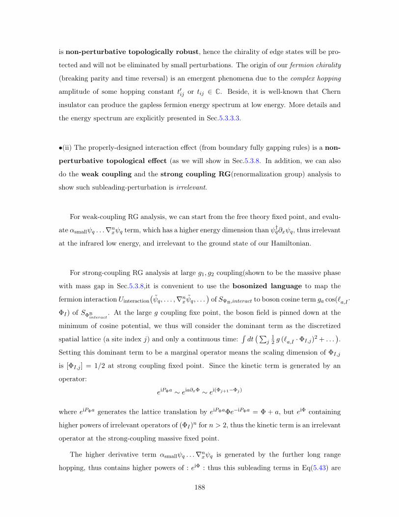
is non-perturbative topologically robust, hence the chirality of edge states will be pro-
tected and will not be eliminated by small perturbations. The origin of our fermion chirality
(breaking parity and time reversal) is an emergent phenomena due to the complex hopping
amplitude of some hopping constant 𝑡′𝑖𝑗 or 𝑡𝑖𝑗 ∈ C. Beside, it is well-known that Chern
insulator can produce the gapless fermion energy spectrum at low energy. More details and
the energy spectrum are explicitly presented in Sec.5.3.3.3.
∙(ii) The properly-designed interaction effect (from boundary fully gapping rules) is a non-
perturbative topological effect (as we will show in Sec.5.3.8. In addition, we can also
do the weak coupling and the strong coupling RG(renormalization group) analysis to
show such subleading-perturbation is irrelevant.
For weak-coupling RG analysis, we can start from the free theory fixed point, and evalu-
ate 𝛼small𝜓𝑞 . . .∇𝑛𝑥𝜓𝑞 term, which has a higher energy dimension than 𝜓†𝑞𝜕𝑥𝜓𝑞, thus irrelevant
at the infrared low energy, and irrelevant to the ground state of our Hamiltonian.
For strong-coupling RG analysis at large 𝑔1, 𝑔2 coupling(shown to be the massive phase
with mass gap in Sec.5.3.8,it is convenient to use the bosonized language to map the
fermion interaction 𝑈interaction(𝜓𝑞, . . . ,∇𝑛𝑥𝜓𝑞, . . .
)of 𝑆ΨB,𝑖𝑛𝑡𝑒𝑟𝑎𝑐𝑡 to boson cosine term 𝑔𝑎 cos(ℓ𝑎,𝐼 ·
Φ𝐼) of 𝑆ΦB𝑖𝑛𝑡𝑒𝑟𝑎𝑐𝑡
. At the large 𝑔 coupling fixe point, the boson field is pinned down at the
minimum of cosine potential, we thus will consider the dominant term as the discretized
spatial lattice (a site index 𝑗) and only a continuous time:∫𝑑𝑡
(∑𝑗12 𝑔 (ℓ𝑎,𝐼 ·Φ𝐼,𝑗)
2 + . . .).
Setting this dominant term to be a marginal operator means the scaling dimension of Φ𝐼,𝑗
is [Φ𝐼,𝑗 ] = 1/2 at strong coupling fixed point. Since the kinetic term is generated by an
operator:
𝑒i𝑃Φ𝑎 ∼ 𝑒i𝑎𝜕𝑥Φ ∼ 𝑒i(Φ𝑗+1−Φ𝑗)
where 𝑒i𝑃Φ𝑎 generates the lattice translation by 𝑒i𝑃Φ𝑎Φ𝑒−i𝑃Φ𝑎 = Φ + 𝑎, but 𝑒iΦ containing
higher powers of irrelevant operators of (Φ𝐼)𝑛 for 𝑛 > 2, thus the kinetic term is an irrelevant
operator at the strong-coupling massive fixed point.
The higher derivative term 𝛼small𝜓𝑞 . . .∇𝑛𝑥𝜓𝑞 is generated by the further long range
hopping, thus contains higher powers of : 𝑒iΦ : thus this subleading terms in Eq(5.43) are
188
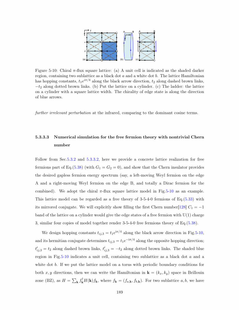
b!
a!
A B
(a) (b) (c)
A B x
y
x
y
Figure 5-10: Chiral 𝜋-flux square lattice: (a) A unit cell is indicated as the shaded darkerregion, containing two sublattice as a black dot 𝑎 and a white dot 𝑏. The lattice Hamiltonianhas hopping constants, 𝑡1𝑒𝑖𝜋/4 along the black arrow direction, 𝑡2 along dashed brown links,−𝑡2 along dotted brown links. (b) Put the lattice on a cylinder. (c) The ladder: the latticeon a cylinder with a square lattice width. The chirality of edge state is along the directionof blue arrows.
further irrelevant perturbation at the infrared, comparing to the dominant cosine terms.
5.3.3.3 Numerical simulation for the free fermion theory with nontrivial Chern
number
Follow from Sec.5.3.2 and 5.3.3.2, here we provide a concrete lattice realization for free
fermions part of Eq.(5.38) (with 𝐺1 = 𝐺2 = 0), and show that the Chern insulator provides
the desired gapless fermion energy spectrum (say, a left-moving Weyl fermion on the edge
A and a right-moving Weyl fermion on the edge B, and totally a Dirac fermion for the
combined). We adopt the chiral 𝜋-flux square lattice model in Fig.5-10 as an example.
This lattice model can be regarded as a free theory of 3-5-4-0 fermions of Eq.(5.33) with
its mirrored conjugate. We will explicitly show filling the first Chern number[128] 𝐶1 = −1
band of the lattice on a cylinder would give the edge states of a free fermion with U(1) charge
3, similar four copies of model together render 3-5-4-0 free fermions theory of Eq.(5.38).
We design hopping constants 𝑡𝑖𝑗,3 = 𝑡1𝑒i𝜋/4 along the black arrow direction in Fig.5-10,
and its hermitian conjugate determines 𝑡𝑖𝑗,3 = 𝑡1𝑒−i𝜋/4 along the opposite hopping direction;
𝑡′𝑖𝑗,3 = 𝑡2 along dashed brown links, 𝑡′𝑖𝑗,3 = −𝑡2 along dotted brown links. The shaded blue
region in Fig.5-10 indicates a unit cell, containing two sublattice as a black dot 𝑎 and a
white dot 𝑏. If we put the lattice model on a torus with periodic boundary conditions for
both 𝑥, 𝑦 directions, then we can write the Hamiltonian in k = (𝑘𝑥, 𝑘𝑦) space in Brillouin
zone (BZ), as 𝐻 =∑
k 𝑓†k𝐻(k)𝑓k, where 𝑓k = (𝑓𝑎,k, 𝑓𝑏,k). For two sublattice 𝑎, 𝑏, we have
189
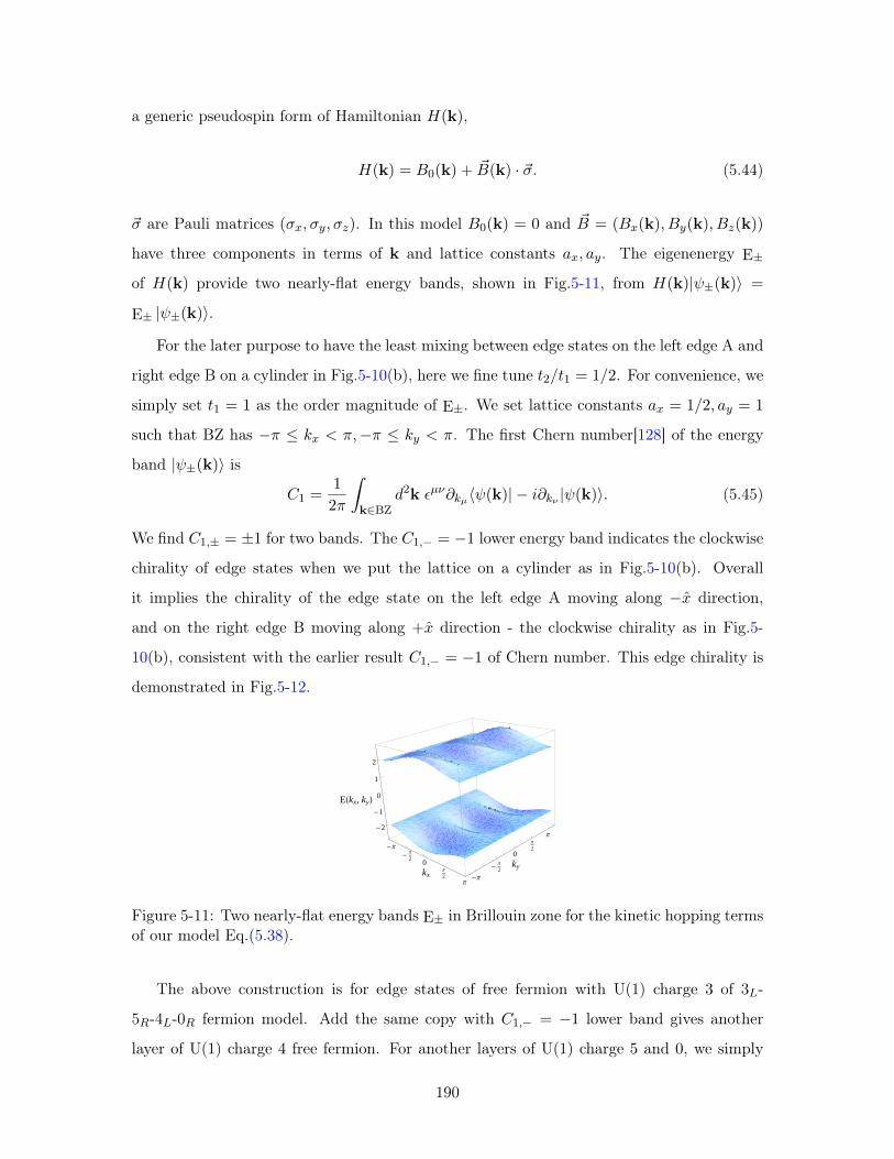
a generic pseudospin form of Hamiltonian 𝐻(k),
𝐻(k) = 𝐵0(k) + ��(k) · ��. (5.44)
�� are Pauli matrices (𝜎𝑥, 𝜎𝑦, 𝜎𝑧). In this model 𝐵0(k) = 0 and �� = (𝐵𝑥(k), 𝐵𝑦(k), 𝐵𝑧(k))
have three components in terms of k and lattice constants 𝑎𝑥, 𝑎𝑦. The eigenenergy E±
of 𝐻(k) provide two nearly-flat energy bands, shown in Fig.5-11, from 𝐻(k)|𝜓±(k)⟩ =
E± |𝜓±(k)⟩.
For the later purpose to have the least mixing between edge states on the left edge A and
right edge B on a cylinder in Fig.5-10(b), here we fine tune 𝑡2/𝑡1 = 1/2. For convenience, we
simply set 𝑡1 = 1 as the order magnitude of E±. We set lattice constants 𝑎𝑥 = 1/2, 𝑎𝑦 = 1
such that BZ has −𝜋 ≤ 𝑘𝑥 < 𝜋,−𝜋 ≤ 𝑘𝑦 < 𝜋. The first Chern number[128] of the energy
band |𝜓±(k)⟩ is
𝐶1 =1
2𝜋
∫k∈BZ
𝑑2k 𝜖𝜇𝜈𝜕𝑘𝜇⟨𝜓(k)| − 𝑖𝜕𝑘𝜈 |𝜓(k)⟩. (5.45)
We find 𝐶1,± = ±1 for two bands. The 𝐶1,− = −1 lower energy band indicates the clockwise
chirality of edge states when we put the lattice on a cylinder as in Fig.5-10(b). Overall
it implies the chirality of the edge state on the left edge A moving along −�� direction,
and on the right edge B moving along +�� direction - the clockwise chirality as in Fig.5-
10(b), consistent with the earlier result 𝐶1,− = −1 of Chern number. This edge chirality is
demonstrated in Fig.5-12.
-Π
-Π
20
Π
2Π
kx -Π
-Π
2
0
Π
2
Π
ky
-2
-1
0
1
2
EHkx, kyL
Figure 5-11: Two nearly-flat energy bands E± in Brillouin zone for the kinetic hopping termsof our model Eq.(5.38).
The above construction is for edge states of free fermion with U(1) charge 3 of 3𝐿-
5𝑅-4𝐿-0𝑅 fermion model. Add the same copy with 𝐶1,− = −1 lower band gives another
layer of U(1) charge 4 free fermion. For another layers of U(1) charge 5 and 0, we simply
190
adjust hopping constant 𝑡𝑖𝑗 to 𝑡1𝑒−i𝜋/4 along the black arrow direction and 𝑡1𝑒i𝜋/4 along the
opposite direction in Fig.5-10, which makes 𝐶1,− = +1. Stack four copies of chiral 𝜋-flux
ladders with 𝐶1,− = −1,+1,−1,+1 provides the lattice model of 3-5-4-0 free fermions with
its mirrored conjugate.
The lattice model so far is an effective 1+1D non-chiral theory. We claim the interaction
terms (𝐺1, 𝐺2 = 0) can gap out the mirrored edge states on the edge B. The simulation
including interactions can be numerically expansive, even so on a simple ladder model. Be-
cause of higher power interactions, one can no longer diagonalize the model in k space as the
case of the quadratic free-fermion Hamiltonian. For interacting case, one may need to apply
exact diagonalization in real space, or density matrix renormalization group (DMRG), which
is powerful in 1+1D. We leave this interacting numerical study for the lattice community or
the future work.
(a) -Π -Π
20 Π
2Π
-2
-1
0
1
2
kx
EHkxL
(b) -Π -Π
20 Π
2Π
-2
-1
0
1
2
kx
EHkxL
(c) -Π - Π
20 Π
2Π
0
12
1
kx
Density X fA† fA\ and X fB
† fB\ on the Edge
Figure 5-12: The energy spectrum E(𝑘𝑥) and the density matrix ⟨𝑓 †𝑓⟩ of the chiral 𝜋-fluxmodel on a cylinder: (a) On a 10-sites width (9𝑎𝑦-width) cylinder: The blue curves areedge states spectrum. The black curves are for states extending in the bulk. The chemicalpotential at zero energy fills eigenstates in solid curves, and leaves eigenstates in dashedcurves unfilled. (b) On the ladder, a 2-sites width (1𝑎𝑦-width) cylinder: the same as the(a)’s convention. (c) The density ⟨𝑓 †𝑓⟩ of the edge eigenstates (the solid blue curve in (b))on the ladder lattice. The dotted blue curve shows the total density sums to 1, the darkerpurple curve shows ⟨𝑓 †A𝑓A⟩ on the left edge A, and the lighter purple curve shows ⟨𝑓 †B𝑓B⟩on the right edge B. The dotted darker(or lighter) purple curve shows density ⟨𝑓 †A,𝑎𝑓A,𝑎⟩ (or⟨𝑓 †B,𝑎𝑓B,𝑎⟩) on sublattice 𝑎, while the dashed darker(or lighter) purple curve shows density⟨𝑓 †
A,𝑏𝑓A,𝑏⟩ (or ⟨𝑓 †
B,𝑏𝑓B,𝑏⟩) on sublattice 𝑏. This edge eigenstate has the left edge A density
with majority quantum number 𝑘𝑥 < 0, and has the right edge B density with majorityquantum number 𝑘𝑥 > 0. Densities on two sublattice 𝑎, 𝑏 are equally distributed as wedesire.
191
5.3.4 Interaction gapping terms and the strong coupling scale
Similar to Sec.5.3.3.2, for the interaction gapping terms of the Hamiltonian, we can do
the mapping based on Eq.(5.43), where the leading terms on the lattice is
𝑔𝑎 cos(ℓ𝑎,𝐼 · Φ𝐼) = 𝑈interaction(𝜓𝑞, . . . ,∇𝑛𝑥𝜓𝑞, . . .
))→ 𝑈point.split.
(𝑓𝑞(𝑗), . . .
(𝑓𝑛𝑞 (𝑗)
)𝑝𝑡.𝑠.
, . . .
)+ 𝛼small . . . (5.46)
Again, potentially there may contain subleading pieces, such as further higher order deriva-
tives 𝛼small∇𝑛𝑥𝜓𝑞 with a small coefficient 𝛼small, or tiny mixing of the different U(1)-charge
flavors 𝛼′small𝜓𝑞1𝜓𝑞2 . . .. However, using the same RG analysis in Sec.5.3.3.2, at both the
weak coupling and the strong coupling fix points, we learn that those 𝛼small terms are only
subleading-perturbative effects which are further irrelevant perturbation at the infrared
comparing to the dominant piece (which is the kinetic term for the weak 𝑔 coupling, but is
replaced by the cosine term for the strong 𝑔 coupling).
One more question to ask is: what is the scale of coupling 𝐺 such that the gapping
term becomes dominant and the B edge states form the mass gaps, but maintaining
(without interfering with) the gapless A edge states?
To answer this question, we first know the absolute value of energy magnitude for each
term in the desired Hamiltonian for our chiral fermion model:
|𝐺 gapping term| & |𝑡𝑖𝑗 , 𝑡′𝑖𝑗 kinetic term| (5.47)
≫ |𝐺 higher order ∇𝑛𝑥 and mixing terms| ≫ |𝑡𝑖𝑗 , 𝑡′𝑖𝑗 higher order 𝜓𝑞 . . .∇𝑛𝑥𝜓𝑞|.
For field theory, the gapping terms (the cosine potential term or the multi-fermion
interactions) are irrelevant for a weak 𝑔 coupling, this implies that 𝑔 needs to be large
enough. Here the 𝑔 ≡ (𝑔𝑎)/𝑎2 really means the dimensionless quantity 𝑔𝑎.
For lattice model, however, the dimensional analysis is very different. Since the 𝐺
coupling of gapping terms and the hopping amplitude 𝑡𝑖𝑗 both have dimension of energy
[𝐺] = [𝑡𝑖𝑗 ] = 1, this means that the scale of the dimensionless quantity of |𝐺|/|𝑡𝑖𝑗 | is
important. (The |𝑡𝑖𝑗 |, |𝑡′𝑖𝑗 | are about the same order of magnitude.)
Presumably we can design the lattice model under Eq.(5.41), 𝑎 < 𝜉 < 𝑤 < 𝐿, such that
their ratios between each length scale are about the same. We expect the ratio of couplings
of |𝐺| to |𝑡𝑖𝑗 | is about the ratio of mass gap Δ𝑚 to kinetic energy fluctuation 𝛿𝐸𝑘 caused by
192
𝑡𝑖𝑗 hopping, thus very roughly
|𝐺||𝑡𝑖𝑗 |∼ Δ𝑚
𝛿𝐸𝑘∼ (𝜉)−1
(𝑤)−1∼ 𝑤
𝜉∼ 𝐿
𝑤∼ 𝜉
𝑎. (5.48)
We expect that the scales at strong coupling 𝐺 is about
|𝐺| & |𝑡𝑖𝑗 | ·𝜉
𝑎(5.49)
this magnitude can support our lattice chiral fermion model with mirror-fermion decoupling.
If 𝐺 is too much smaller than |𝑡𝑖𝑗 | · 𝜉𝑎 , then mirror sector stays gapless. On the other hand,
if |𝐺|/|𝑡𝑖𝑗 | is too much stronger or simply |𝐺|/|𝑡𝑖𝑗 | → ∞ may cause either of two disastrous
cases:
(i) Both edges would be gapped and the whole 2D plane becomes dead without kinetic
hopping, if the correlation length reaches the scale of the cylinder width: 𝜉 & 𝑤.
(ii) The B edge(say at site 𝑛𝑦) becomes completely gapped, but forms a dead overly-high-
energy 1D line decoupled from the remain lattice. The neighbored line (along (𝑛−1)𝑦) next
to edge B experiences no interaction thus may still form mirror gapless states near B. (This
may be another reason why CGP fails in Ref.[125] due to implementing overlarge strong
coupling.)
So either the two cases caused by too much strong |𝐺|/|𝑡𝑖𝑗 | is not favorable. Only |𝐺| &
|𝑡𝑖𝑗 | · 𝜉𝑎 , we can have the mirrored sector at edge 𝐵 gapped, meanwhile keep the chiral
sector at edge 𝐴 gapless. |𝐺||𝑡𝑖𝑗 | is somehow larger than order 1 is what we referred as the
intermediate(-strong) coupling.
|𝐺||𝑡𝑖𝑗 |& 𝑂(1). (5.50)
(Our 𝑂(1) means some finite values, possibly as large as 104, 106, etc, but still finite. And
the kinetic term is not negligible.) The sign of 𝐺 coupling shall not matter, since in the
cosine potential language, either 𝑔1, 𝑔2 greater or smaller than zero are related by sifting the
minimum energy vaccua of the cosine potential.
To summarize, the two key messages in Sec.5.3.3 are:
∙ First, the free-kinetic hopping part of lattice model has been simulated and there gapless
193
energy spectra have been computed shown in Figures. The energy spectra indeed show
the gapless Weyl fermions on each edge. So, the continuum field theory to a lattice model
mapping is immaterial to the subleading terms of Eq.(5.43), the physics is as good or as
exact as we expect for the free kinetic part. We comment that this lattice realization of
quantum hall-like states with chiral edges have been implemented for long in condensed
matter, dated back as early such as Haldane’s work.[?]
∙ Second, by adding the interaction gapping terms, the spectra will be modified from the
mirror gapless edge to the mirror gapped edge. The continuum field theory to a lattice model
mapping based on Eq.(5.43) for the gapping terms in Eq.(5.46) is as good or as exact as the
free kinetic part Eq.(5.42), because the mapping is the same procedure as in Eq.(5.43). Since
the subleading correction for the free and for the interacting parts are further irrelevant
perturbation at the infrared, the non-perturbative topological effect of the gapped edge
contributed from the leading terms remains.
In the next section, we will provide a topological non-perturbative proof to justify
that the 𝐺1, 𝐺2 interaction terms can gap out mirrored edge states, without employing
numerical methods, but purely based on an analytical derivation.
5.3.5 Topological Non-Perturbative Proof of Anomaly Matching Condi-
tions = Boundary Fully Gapping Rules
As Sec.5.3.2,5.3.3 prelude, we now show that Eq.(5.38) indeed gaps out the mirrored edge
states on the edge B in Fig.5-9. This proof will support the evidence that Eq.(5.38) gives
the non-perturbative lattice definition of the 1+1D chiral fermion theory of Eq.(5.33).
In Sec.5.3.6, we first provide a generic way to formulate our model, with a insulating bulk
but with gapless edge states. This can be done through so called the bulk-edge correspon-
dence, namely the Chern-Simons theory in the bulk and the Wess-Zumino-Witten(WZW)
model on the boundary. More specifically, for our case with U(1) symmetry chiral mat-
ter theory, we only needs a U(1)𝑁 rank-𝑁 Abelian K matrix Chern-Simons theory in the
bulk and the multiplet chiral boson theory on the boundary. We can further fermionize the
multiplet chiral boson theory to the multiplet chiral fermion theory.
In Sec.5.3.7, we provide a physical understanding between the anomaly matching con-
ditions and the effective Hall conductance. This intuition will be helpful to understand the
relation between the anomaly matching conditions and Boundary Fully Gapping Rules, to
194
be discussed in Sec.5.3.8.
5.3.6 Bulk-Edge Correspondence - 2+1D Bulk Abelian SPT by Chern-
Simons theory
With our 3𝐿-5𝑅-4𝐿-0𝑅 chiral fermion model in mind, below we will trace back to fill in
the background how we obtain this model from the understanding of symmetry-protected
topological states (SPT). This understanding in the end leads to a more general construction.
We first notice that the bosonized action of the free part of chiral fermions in Eq.(5.35),
can be regarded as the edge states action 𝑆𝜕 of a bulk U(1)𝑁 Abelian K matrix Chern-Simons
theory 𝑆𝑏𝑢𝑙𝑘 (on a 2+1D manifoldℳ with the 1+1D boundary 𝜕ℳ):
𝑆𝑏𝑢𝑙𝑘 =𝐾𝐼𝐽
4𝜋
∫ℳ𝑎𝐼 ∧ 𝑑𝑎𝐽 =
𝐾𝐼𝐽
4𝜋
∫ℳ𝑑𝑡 𝑑2𝑥𝜀𝜇𝜈𝜌𝑎𝐼𝜇𝜕𝜈𝑎
𝐽𝜌 , (5.51)
𝑆𝜕 =1
4𝜋
∫𝜕ℳ
𝑑𝑡 𝑑𝑥 𝐾𝐼𝐽𝜕𝑡Φ𝐼𝜕𝑥Φ𝐽 − 𝑉𝐼𝐽𝜕𝑥Φ𝐼𝜕𝑥Φ𝐽 . (5.52)
Here 𝑎𝜇 is intrinsic 1-form gauge field from a low energy viewpoint. Both indices 𝐼, 𝐽 run
from 1 to 𝑁 . Given 𝐾𝐼𝐽 matrix, it is known the ground state degeneracy (GSD) of this
theory on the T2 torus is GSD = | det𝐾|.Here 𝑉𝐼𝐽 is the symmetric ‘velocity’ matrix, we
can simply choose 𝑉𝐼𝐽 = I, without losing generality of our argument. The U(1)𝑁 gauge
transformation is 𝑎𝐼 → 𝑎𝐼 + 𝑑𝑓𝐼 and Φ𝐼 → Φ𝐼 + 𝑓𝐼 . The bulk-edge correspondence is meant
to have the gauge non-invariances of the bulk-only and the edge-only cancel with each other,
so that the total gauge invariances is achieved from the full bulk and edge as a whole.
We will consider only an even integer 𝑁 ∈ 2Z+. The reason is that only such even
number of edge modes, we can potentially gap out the edge states. (For odd integer 𝑁 , such
a set of gapping interaction terms generically do not exist, so the mirror edge states remain
gapless.)
To formulate 3𝐿-5𝑅-4𝐿-0𝑅 fermion model, as shown in Eq.(5.35), we need a rank-4 K
matrix(1 00 −1
)⊕(1 00 −1
). Generically, for a general U(1) chiral fermion model, we can use a
canonical fermionic matrix
𝐾𝑓𝑁×𝑁 =
(1 00 −1
)⊕(1 00 −1
)⊕(1 00 −1
)⊕ . . . (5.53)
Such a matrix is special, because it describes a more-restricted Abelian Chern-Simons theory
195
with GSD= |det𝐾𝑓𝑁×𝑁 | = 1 on the T2 torus. In the condensed matter language, the uniques
GSD implies it has no long range entanglement, and it has no intrinsic topological order.
Such a state may be wronged to be only a trivial insulator, but actually this is recently-
known to be potentially nontrivial as the symmetry-protected topological states (SPT).
(This paragraph is for readers with interests in SPT: SPT are short-range entangled
states with onsite symmetry in the bulk. For SPT, there is no long-range entanglement,
no fractionalized quasiparticles (fractional anyons) and no fractional statistics in the bulk.
The bulk onsite symmetry may be realized as a non-onsite symmetry on the boundary. If
one gauges the non-onsite symmetry of the boundary SPT, the boundary theory becomes
an anomalous gauge theory.[127] The anomalous gauge theory is ill-defined in its own di-
mension, but can be defined as the boundary of the bulk SPT. However, this understanding
indicates that if the boundary theory happens to be anomaly-free, then it can be defined
non-perturbatively on the same dimensional lattice.)
𝐾𝑓𝑁×𝑁 matrix describe fermionic SPT states, which is described by bulk spin Chern-
Simons theory of |det𝐾| = 1. A spin Chern-Simons theory only exist on the spin manifold,
which has spin structure and can further define spinor bundles. However, there are another
simpler class of SPT states, the bosonic SPT states, which is described by the canonical
form 𝐾𝑏±𝑁×𝑁 with blocks of
(0 11 0
)and a set of all positive(or negative) coefficients E8 lattices
𝐾E8 , namely,
𝐾𝑏0𝑁×𝑁 =
(0 11 0
)⊕(0 11 0
)⊕ . . . . (5.54)
𝐾𝑏±𝑁×𝑁 = 𝐾𝑏0 ⊕ (±𝐾E8)⊕ (±𝐾E8)⊕ . . .
The 𝐾E8 matrix describe 8-multiplet chiral bosons moving in the same direction, thus it
cannot be gapped by adding multi-fermion interaction among themselves. We will neglect
E8 chiral boson states but only focus on 𝐾𝑏0𝑁×𝑁 for the reason to consider only the gappable
states. The K-matrix form of Eq.(5.53),(5.54) is called the unimodular indefinite symmetric
integral matrix.
After fermionizing the boundary action Eq.(5.52) with 𝐾𝑓𝑁×𝑁 matrix, we obtain multi-
plet chiral fermions (with several pairs, each pair contain left-right moving Weyl fermions
196
forming a Dirac fermion).
𝑆Ψ =
∫𝜕ℳ
𝑑𝑡 𝑑𝑥 (iΨAΓ𝜇𝜕𝜇ΨA). (5.55)
with Γ0 =𝑁/2⨁𝑗=1
𝛾0, Γ1 =𝑁/2⨁𝑗=1
𝛾1, Γ5 ≡ Γ0Γ1, Ψ𝑖 ≡ Ψ𝑖Γ0 and 𝛾0 = 𝜎𝑥, 𝛾1 = i𝜎𝑦, 𝛾5 ≡ 𝛾0𝛾1 =
−𝜎𝑧.
Symmetry transformation for the edge states-
The edge states of 𝐾𝑓𝑁×𝑁 and 𝐾𝑏0
𝑁×𝑁 Chern-Simons theory are non-chiral in the sense
there are equal number of left and right moving modes. However, we can make them with
a charged ‘chirality’ respect to a global(or external probed, or dynamical gauge) symmetry
group. For the purpose to build up our ‘chiral fermions and chiral bosons’ model with ‘charge
chirality,’ we consider the simplest possibility to couple it to a global U(1) symmetry with
a charge vector t. (This is the same as the symmetry charge vector of SPT states[66, 67])
Chiral Bosons: For the case of multiplet chiral boson theory of Eq.(5.52), the group
element 𝑔𝜃 of U(1) symmetry acts on chiral fields as
𝑔𝜃 :𝑊U(1)𝜃 = I𝑁×𝑁 , 𝛿𝜑U(1)𝜃 = 𝜃t, (5.56)
With the following symmetry transformation,
𝜑→𝑊U(1)𝜃𝜑+ 𝛿𝜑U(1)𝜃 = 𝜑+ 𝜃t (5.57)
To derive this boundary symmetry transformation from the bulk Chern-Simons theory
via bulk-edge correspondence, we first write down the charge coupling bulk Lagrangian
term, namely q𝐼
2𝜋 𝜖𝜇𝜈𝜌𝐴𝜇𝜕𝜈𝑎𝐼𝜌, where the global symmetry current q𝐼𝐽𝐼𝜇 = q𝐼
2𝜋 𝜖𝜇𝜈𝜌𝜕𝜈𝑎𝐼𝜌 is
coupled to an external gauge field 𝐴𝜇. The bulk U(1)-symmetry current q𝐼𝐽𝐼𝜇 induces a
boundary U(1)-symmetry current 𝑗𝐼𝜇 = q𝐼
2𝜋 𝜖𝜇𝜈𝜕𝜈𝜑𝐼 . This implies the boundary symmetry
operator is 𝑆𝑠𝑦𝑚 = exp(i 𝜃 q𝐼
2𝜋
∫𝜕𝑥𝜑𝐼), with an arbitrary U(1) angle 𝜃 The induced symmetry
transformation on 𝜑𝐼 is:
(𝑆𝑠𝑦𝑚)𝜑𝐼(𝑆𝑠𝑦𝑚)−1 = 𝜑𝐼 − i𝜃
∫𝑑𝑥
q𝑙
2𝜋[𝜑𝐼 , 𝜕𝑥𝜑𝑙] = 𝜑𝐼 + 𝜃(𝐾−1)𝐼𝑙q
𝑙 ≡ 𝜑𝐼 + 𝜃t𝐼 , (5.58)
197
here we have used the canonical commutation relation [𝜑𝐼 , 𝜕𝑥𝜑𝑙] = i (𝐾−1)𝐼𝑙. Compare the
two Eq.(5.57),(5.58), we learn that
t𝐼 ≡ (𝐾−1)𝐼𝑙q𝑙.
The charge vectors t𝐼 and q𝑙 are related by an inverse of the 𝐾 matrix. The generic
interacting or gapping terms[60, 68, 66] for the multiplet chiral boson theory are the sine-
Gordon or the cosine term
𝑆𝜕,gap =
∫𝑑𝑡 𝑑𝑥
∑𝑎
𝑔𝑎 cos(ℓ𝑎,𝐼 · Φ𝐼). (5.59)
If we insist that 𝑆𝜕,gap obeys U(1) symmetry, to make Eq.(5.59) invariant under Eq.(5.58),
we have to impose
ℓ𝑎,𝐼 · Φ𝐼 → ℓ𝑎,𝐼 · (Φ𝐼 + 𝛿𝜑U(1)𝜃)mod 2𝜋
so ℓ𝑎,𝐼 · t𝐼 = 0 ⇒ ℓ𝑎,𝐼 · (𝐾−1)𝐼𝑙 · q𝑙 = 0 . (5.60)
The above generic U(1) symmetry transformation works for bosonic 𝐾𝑏0𝑁×𝑁 as well as
fermionic 𝐾𝑓𝑁×𝑁 .
Chiral Fermions: In the case of fermionic𝐾𝑓𝑁×𝑁 , we will do one more step to fermionize the
multiplet chiral boson theory. Fermionize the free kinetic part from Eq.(5.52) to Eq.(5.55),
as well as the interacting cosine term:
𝑔𝑎 cos(ℓ𝑎,𝐼 · Φ𝐼)→𝑁∏𝐼=1
𝑔𝑎((𝜓𝑞𝐼 )(∇𝑥𝜓𝑞𝐼 ) . . . (∇
|ℓ𝑎,𝐼 |−1𝑥 𝜓𝑞𝐼 )
)𝜖 ≡ 𝑈interaction(𝜓𝑞, . . . ,∇𝑛𝑥𝜓𝑞, . . .
)(5.61)
to multi-fermion interaction. The 𝜖 is defined as the complex conjugation operator which
depends on sgn(ℓ𝑎,𝐼), the sign of ℓ𝑎,𝐼 . When sgn(ℓ𝑎,𝐼) = −1, we define 𝜓𝜖 ≡ 𝜓† and also
for the higher power polynomial terms. Again, we absorb the normalization factor and the
Klein factors through normal ordering of bosonization into the factor 𝑔𝑎. The precise factor
is not of our concern, since our goal is a non-perturbative lattice model. Obviously, the U(1)
symmetry transformation for fermions is
𝜓𝑞𝐼 → 𝜓𝑞𝐼𝑒it𝐼𝜃 = 𝜓𝑞𝐼𝑒
i(𝐾−1)𝐼𝑙·q𝑙.𝜃 (5.62)
198
In summary, we have shown a framework to describe U(1) symmetry chiral fermion/boson
model using the bulk-edge correspondence, the explicit Chern-Siomns/WZW actions are
given in Eq.(5.51), (5.52), (5.55), (5.59), (5.61), and their symmetry realization Eq.(5.58),(5.62)
and constrain are given in Eq.(5.60),(5.60). Their physical properties are tightly associated
to the fermionic/bosonic SPT states.
5.3.7 Anomaly Matching Conditions and Effective Hall Conductance
The bulk-edge correspondence is meant, not only to achieve the gauge invariance by canceling
the non-invariance of bulk-only and boundary-only, but also to have the boundary anomalous
current flow can be transported into the extra dimensional bulk. This is known as Callan-
Harvey effect in high energy physics, Laughlin thought experiment, or simply the quantum-
hall-like state bulk-edge correspondence in condensed matter theory.
The goal of this subsection is to provide a concrete physical understanding of the anomaly
matching conditions and effective Hall conductance :
∙ (i) The anomalous current inflowing from the boundary is transported into the bulk.
We now show that this thinking can easily derive the 1+1D U(1) Adler-Bell-Jackiw(ABJ)
anomaly, or Schwinger’s 1+1D quantum electrodynamics(QED) anomaly.
We will focus on the U(1) chiral anomaly, which is ABJ anomaly[58, 59] type. It is well-
known that ABJ anomaly can be captured by the anomaly factor 𝒜 of the 1-loop polygon
Feynman diagrams (see Fig.5-13). The anomaly matching condition requires
𝒜 = tr[𝑇 𝑎𝑇 𝑏𝑇 𝑐 . . . ] = 0. (5.63)
Here 𝑇 𝑎 is the (fundamental) representation of the global or gauge symmetry algebra, which
contributes to the vertices of 1-loop polygon Feynman diagrams.
For example, the 3+1D chiral anomaly 1-loop triangle diagram of U(1) symmetry in
Fig.5-13(a) with chiral fermions on the loop gives 𝒜 =∑
(𝑞3𝐿 − 𝑞3𝑅). Similarly, the 1+1D
chiral anomaly 1-loop diagram of U(1) symmetry in Fig.5-13(b) with chiral fermions on the
loop gives 𝒜 =∑
(𝑞2𝐿 − 𝑞2𝑅). Here 𝐿,𝑅 stand for left-moving and right-moving modes.
How to derive this anomaly matching condition from a condensed matter theory view-
point? Conceptually, we understand that
199
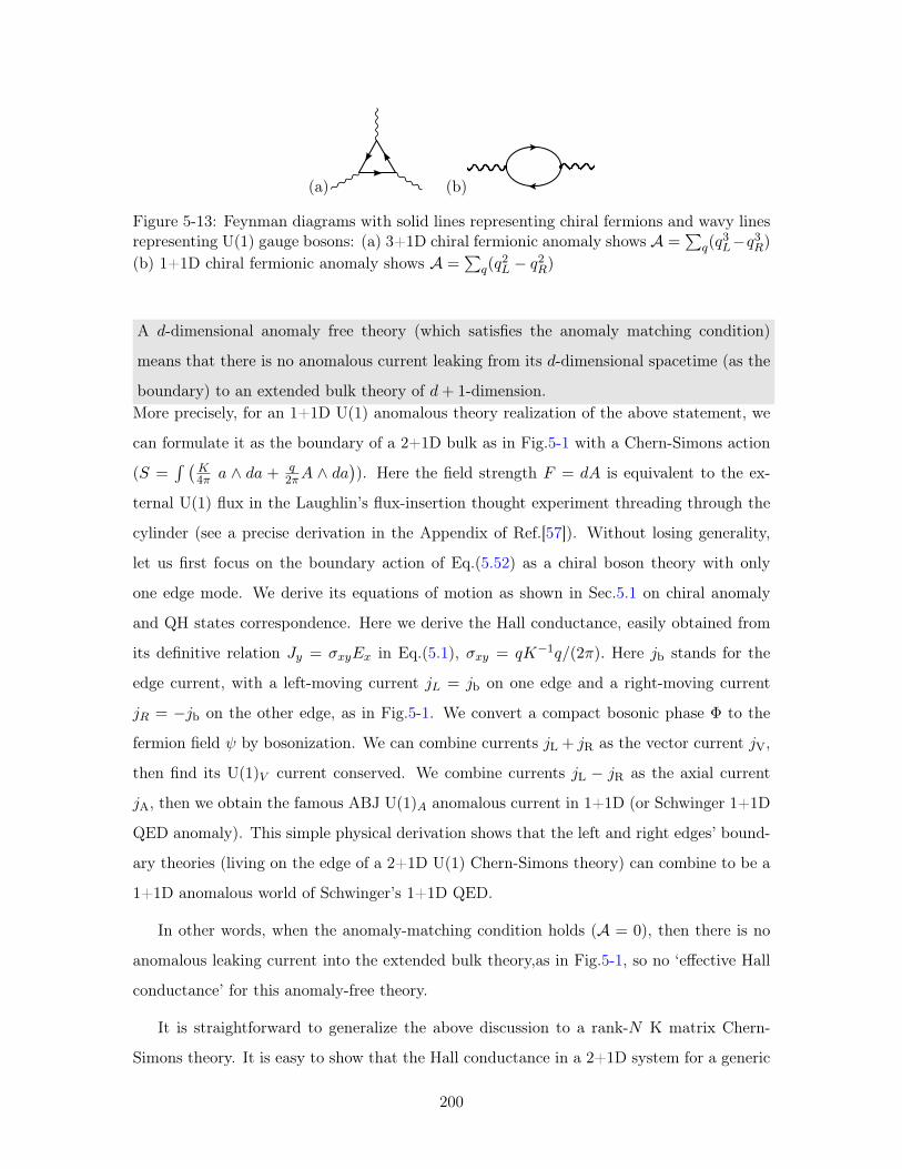
(a) (b)
Figure 5-13: Feynman diagrams with solid lines representing chiral fermions and wavy linesrepresenting U(1) gauge bosons: (a) 3+1D chiral fermionic anomaly shows 𝒜 =
∑𝑞(𝑞
3𝐿−𝑞3𝑅)
(b) 1+1D chiral fermionic anomaly shows 𝒜 =∑
𝑞(𝑞2𝐿 − 𝑞2𝑅)
A 𝑑-dimensional anomaly free theory (which satisfies the anomaly matching condition)
means that there is no anomalous current leaking from its 𝑑-dimensional spacetime (as the
boundary) to an extended bulk theory of 𝑑+ 1-dimension.More precisely, for an 1+1D U(1) anomalous theory realization of the above statement, we
can formulate it as the boundary of a 2+1D bulk as in Fig.5-1 with a Chern-Simons action
(𝑆 =∫ (
𝐾4𝜋 𝑎 ∧ 𝑑𝑎 + 𝑞
2𝜋𝐴 ∧ 𝑑𝑎)). Here the field strength 𝐹 = 𝑑𝐴 is equivalent to the ex-
ternal U(1) flux in the Laughlin’s flux-insertion thought experiment threading through the
cylinder (see a precise derivation in the Appendix of Ref.[57]). Without losing generality,
let us first focus on the boundary action of Eq.(5.52) as a chiral boson theory with only
one edge mode. We derive its equations of motion as shown in Sec.5.1 on chiral anomaly
and QH states correspondence. Here we derive the Hall conductance, easily obtained from
its definitive relation 𝐽𝑦 = 𝜎𝑥𝑦𝐸𝑥 in Eq.(5.1), 𝜎𝑥𝑦 = 𝑞𝐾−1𝑞/(2𝜋). Here 𝑗b stands for the
edge current, with a left-moving current 𝑗𝐿 = 𝑗b on one edge and a right-moving current
𝑗𝑅 = −𝑗b on the other edge, as in Fig.5-1. We convert a compact bosonic phase Φ to the
fermion field 𝜓 by bosonization. We can combine currents 𝑗L + 𝑗R as the vector current 𝑗V,
then find its U(1)𝑉 current conserved. We combine currents 𝑗L − 𝑗R as the axial current
𝑗A, then we obtain the famous ABJ U(1)𝐴 anomalous current in 1+1D (or Schwinger 1+1D
QED anomaly). This simple physical derivation shows that the left and right edges’ bound-
ary theories (living on the edge of a 2+1D U(1) Chern-Simons theory) can combine to be a
1+1D anomalous world of Schwinger’s 1+1D QED.
In other words, when the anomaly-matching condition holds (𝒜 = 0), then there is no
anomalous leaking current into the extended bulk theory,as in Fig.5-1, so no ‘effective Hall
conductance’ for this anomaly-free theory.
It is straightforward to generalize the above discussion to a rank-𝑁 K matrix Chern-
Simons theory. It is easy to show that the Hall conductance in a 2+1D system for a generic
200
𝐾 matrix is (via q𝑙 = 𝐾𝐼𝑙 t𝐼)
𝜎𝑥𝑦 =1
2𝜋q ·𝐾−1 · q =
1
2𝜋t ·𝐾 · t. (5.64)
For a 2+1D fermionic system for 𝐾𝑓 matrix of Eq.(5.53),
𝜎𝑥𝑦 =𝑞2
2𝜋t(𝐾𝑓
𝑁×𝑁 )t =1
2𝜋
∑𝑞
(𝑞2𝐿 − 𝑞2𝑅) =1
2𝜋𝒜. (5.65)
Remarkably, this physical picture demonstrates that we can reverse the logic, starting from
the ‘effective Hall conductance of the bulk system’ to derive the anomaly factor from
the relation
𝒜 (anomaly factor) = 2𝜋𝜎𝑥𝑦 (effective Hall conductance) (5.66)
And from the “no anomalous current in the bulk” means that “𝜎𝑥𝑦 = 0”, we can further
understand “the anomaly matching condition 𝒜 = 2𝜋𝜎𝑥𝑦 = 0.”
For the U(1) symmetry case, we can explicitly derive the anomaly matching condition
for fermions and bosons.
5.3.8 Anomaly Matching Conditions and Boundary Fully Gapping Rules
This subsection is the main emphasis of our work, and we encourage the readers paying extra
attentions on the result presented here. We will first present a heuristic physical argument
on the rules that under what situations the boundary states can be gapped, named as the
Boundary Fully Gapping Rules. We will then provide a topological non-perturbative
proof using the notion of Lagrangian subgroup and the exact sequence, following our pre-
vious work Ref.[60] and the work in Ref.[68]. And we will also provide perturbative RG
analysis, both for strong and weak coupling analysis of cosine potential cases.
5.3.8.1 topological non-perturbative proof
The above physical picture is suggestive, but not yet rigorous enough mathematically. Here
we will formulate some topological non-perturbative proofs for Boundary Fully Gapping
Rules, and its equivalence to the anomaly-matching conditions for the case of U(1)
201
symmetry. The first approach is using the topological quantum field theory(TQFT) along
the logic of Ref.[129]. The new ingredient for us is to find the equivalence of the gapped
boundary to the anomaly-matching conditions.
For a field theory, the boundary condition is defined by a Lagrangian submanifold in
the space of Cauchy boundary condition data on the boundary. For a topological gapped
boundary condition of a TQFT with a gauge group, we must choose a Lagrangian subspace
in the Lie algebra of the gauge group. A subspace is Lagrangian if and only if it is both
isotropic and coisotropic.
Specifically, for W be a linear subspace of a finite-dimensional vector space V. Define
the symplectic complement of W to be the subspace W⊥ as
W⊥ = {𝑣 ∈ V | 𝜔(𝑣, 𝑤) = 0, ∀𝑤 ∈W} (5.67)
Here 𝜔 is the symplectic form, in the matrix form 𝜔 =
⎛⎝ 0 1
−1 0
⎞⎠ with 0 and 1 are the block
matrix of the zero and the identity. The symplectic complement W⊥ satisfies: (W⊥)⊥ = W,
dimW + dimW⊥ = dimV. We have:
∙W is Lagrangian if and only if it is both isotropic and coisotropic, namely, if and only if
W = W⊥. In a finite-dimensional V, a Lagrangian subspace W is an isotropic one whose
dimension is half that of V.
Now let us focus on the K-matrix U(1)𝑁 Chern-Simons theory, the symplectic form 𝜔 is
given by (with the restricted 𝑎‖,𝐼 on 𝜕ℳ )
𝜔 =𝐾𝐼𝐽
4𝜋
∫ℳ(𝛿𝑎‖,𝐼) ∧ 𝑑(𝛿𝑎‖,𝐽). (5.68)
The bulk gauge group U(1)𝑁 ∼= TΛ as the torus, is the quotient space of 𝑁 -dimensional
vector space V by a subgroup Λ ∼= Z𝑁 . Locally the gauge field 𝑎 is a 1-form, which has
values in the Lie algebra of TΛ, we can denote this Lie algebra tΛ as the vector space
tΛ = Λ⊗ R.
Importantly, for topological gapped boundary, 𝑎‖,𝐼 lies in a Lagrangian subspace of tΛ
implies that the boundary gauge group (≡ TΛ0) is a Lagrangian subgroup. We can
rephrase it in terms of the exact sequence for the vector space of Abelian group Λ ∼= Z𝑁
202
and its subgroup Λ0:
0→ Λ0h→ Λ→ Λ/Λ0 → 0. (5.69)
Here 0 means the trivial zero-dimensional vector space and h is an injective map from Λ0 to
Λ. We can also rephrase it in terms of the exact sequence for the vector space of Lie algebra
by 0→ t*(Λ/Λ0)→ t*Λ → t*Λ0
→ 0.
The generic Lagrangian subgroup condition applies to K-matrix with the above sym-
plectic form Eq.(5.68) renders three conditions on W:
∙(𝑖) The subspace W is isotropic with respect to the symmetric bilinear form 𝐾.
∙(𝑖𝑖) The subspace dimension is a half of the dimension of tΛ.
∙(𝑖𝑖𝑖) The signature of 𝐾 is zero. This means that 𝐾 has the same number of positive and
negative eigenvalues.
Now we can examine the if and only if conditions ∙(𝑖),∙(𝑖𝑖),∙(𝑖𝑖𝑖) listed above.
For ∙(𝑖) “The subspace is isotropic with respect to the symmetric bilinear form 𝐾” to be
true, we have an extra condition on the injective h matrix (h with 𝑁 × (𝑁/2) components)
for the 𝐾 matrix:
h𝑇𝐾h = 0 . (5.70)
Since 𝐾 is invertible(det(𝐾) = 0), by defining a 𝑁 × (𝑁/2)-component L ≡ 𝐾h, we have
an equivalent condition:
L𝑇𝐾−1L = 0 . (5.71)
For ∙(𝑖𝑖), “the subspace dimension is a half of the dimension of tΛ” is true if Λ0 is a
rank-𝑁/2 integer matrix.
For ∙(𝑖𝑖𝑖), “the signature of 𝐾 is zero” is true, because our 𝐾𝑏0 and fermionic 𝐾𝑓 matrices
implies that we have same number of left moving modes (𝑁/2) and right moving modes
(𝑁/2), with 𝑁 ∈ 2Z+ an even number.
Lo and behold, these above conditions ∙(𝑖),∙(𝑖𝑖),∙(𝑖𝑖𝑖) are equivalent to the boundary
full gapping rules listed earlier. We can interpret ∙(𝑖) as trivial statistics by either writing
203
in the column vector of h matrix (h ≡(𝜂1, 𝜂2, . . . , 𝜂𝑁/2
)with 𝑁 × (𝑁/2)-components):
𝜂𝑎,𝐼′𝐾𝐼′𝐽 ′𝜂𝑏,𝐽 ′ = 0 . (5.72)
or writing in the column vector of L matrix (L ≡(ℓ1, ℓ2, . . . , ℓ𝑁/2
)with 𝑁 × (𝑁/2)-
components):
ℓ𝑎,𝐼𝐾−1𝐼𝐽 ℓ𝑏,𝐽 = 0 . (5.73)
for any ℓ𝑎, ℓ𝑏 ∈ Γ𝜕 ≡ {∑
𝛼 𝑐𝛼ℓ𝛼,𝐼 |𝑐𝛼 ∈ Z} of boundary gapping lattice(Lagrangian subgroup).
Namely, the boundary gapping lattice Γ𝜕 is basically the 𝑁/2-dimensional vector space of
a Chern-Simons lattice spanned by the 𝑁/2-independent column vectors of L matrix (L ≡(ℓ1, ℓ2, . . . , ℓ𝑁/2
)).
Moreover, we can go a step further to relate the above rules equivalent to the anomaly-
matching conditions. By adding the corresponding cosine potential 𝑔𝑎 cos(ℓ𝑎 · Φ) to the
edge states of U(1)𝑁 Chern-Simons theory, we break the symmetry down to
U(1)𝑁 → U(1)𝑁/2.
What are the remained U(1)𝑁/2 symmetry? By Eq.(5.60), this remained U(1)𝑁/2 symmetry
is generated by a number of 𝑁/2 of t𝑏,𝐼 vectors satisfying ℓ𝑎,𝐼 · t𝑏,𝐼 = 0. We can easily
construct
t𝑏,𝐼 ≡ 𝐾−1𝐼𝐽 ℓ𝑏,𝐽 , t ≡ 𝐾−1L (5.74)
with 𝑁/2 number of them (or define t as the linear-combination of t𝑏,𝐼 ≡∑
𝐼′ 𝑐𝐼𝐼′(𝐾−1𝐼′𝐽ℓ𝑏,𝐽)).
It turns out that U(1)𝑁/2 symmetry is exactly generated by t𝑏,𝐼 with 𝑏 = 1, . . . , 𝑁/2, and
these remained unbroken symmetry with 𝑁/2 of U(1) generators are anomaly-free and
mixed anomaly-free, due to
t𝑎,𝐼′𝐾𝐼′𝐽 ′t𝑏,𝐽 ′ = ℓ𝑎,𝐼′𝐾−1𝐼′𝐽 ′ℓ𝑏,𝐽 ′ = 0 . (5.75)
Indeed, t𝑎 must be anomaly-free, because it is easily notice that by defining an 𝑁 × 𝑁/2
matrix t ≡(t1, t2, . . . , t𝑁/2
)=
(𝜂1, 𝜂2, . . . , 𝜂𝑁/2
)of Eq.(5.70), thus we must have:
t𝑇𝐾t = 0 , where t = h. (5.76)
204
This is exactly the anomaly factor and the effective Hall conductance discussed in Sec.5.3.7.
In summary of the above, we have provided a topological non-perturbative proof that
the Boundary Fully Gapping Rules, and its extension to the equivalence relation to
the anomaly-matching conditions. We emphasize that Boundary Fully Gapping
Rules provide a topological statement on the gapped boundary conditions, which is non-
perturbative, while the anomaly-matching conditions are also non-perturbative in the
sense that the conditions hold at any energy scale, from low energy IR to high energy
UV. Thus, the equivalence between the twos is remarkable, especially that both are non-
perturbative statements (namely the proof we provide is as exact as integer number values
without allowing any small perturbative expansion). Our proof apply to a bulk U(1)𝑁 K
matrix Chern-Simons theory (describing bulk Abelian topological orders or Abelian SPT
states) with boundary multiplet chiral boson/fermion theories.
5.3.8.2 perturbative arguments
Apart from the non-perturbative proof using TQFT, we can use other well-known techniques
to show the boundary is gapped when the Boundary Fully Gapping Rules are satisfied.
it is convenient to map the 𝐾𝑁×𝑁 -matrix multiplet chiral boson theory to 𝑁/2 copies of
non-chiral Luttinger liquids, each copy with an action
∫𝑑𝑡 𝑑𝑥
( 1
4𝜋((𝜕𝑡𝜑𝑎𝜕𝑥𝜃𝑎 + 𝜕𝑥𝜑𝑎𝜕𝑡𝜃𝑎)− 𝑉𝐼𝐽𝜕𝑥Φ𝐼𝜕𝑥Φ𝐽) + 𝑔 cos(𝛽 𝜃𝑎)
)(5.77)
at large coupling 𝑔 at the low energy ground state. Notice that the mapping sends Φ →
Φ′′ = (𝜑1, 𝜑2, . . . , 𝜑𝑁/2, 𝜃1, 𝜃2, . . . , 𝜃𝑁/2) in a new basis, such that the cosine potential only
takes one field 𝜃𝑎 decoupled from the full multiplet. However, this mapping has been shown
to be possible if L𝑇𝐾−1L = 0 is satisfied.
When the mapping is done, we can simply study a single copy of non-chiral Luttinger liq-
uids, and which, by changing of variables, is indeed equivalent to the action of Klein-Gordon
fields with a sine-Gordon cosine potential studied by S. Coleman. We have demonstrated
various ways to show the existence of mass gap of this sine-Gordon action For example,
∙ For non-perturbative perspectives, there is a duality between the quantum sine-Gordon
action of bosons and the massive Thirring model of fermions in 1+1D. In the sense, it is
205
an integrable model, and the Zamolodchikov formula is known and Bethe ansatz can be
applicable. The mass gap is known unambiguously at the large 𝑔.
∙ For perturbative arguments, we can use RG to do weak or strong coupling expansions.
For weak coupling 𝑔 analysis, it is known that choosing the kinetic term as a marginal
term, and the scaling dimension of the normal ordered [cos(𝛽𝜃)] = 𝛽2
2 . In the weak coupling
analysis, 𝛽2 < 𝛽2𝑐 ≡ 4 will flow to the large 𝑔 gapped phases (with an exponentially decaying
correlator) at low energy, while 𝛽2 > 𝛽2𝑐 will have the low energy flow to the quasi-long-range
gapless phases (with an algebraic decaying correlator) at the low energy ground state. At
𝛽 = 𝛽𝑐, it is known to have Berezinsky-Kosterlitz-Thouless(BKT) transition. We find that
our model satisfies 𝛽2 < 𝛽2𝑐 , thus necessarily flows to gapped phases, because the gapping
terms can be written as 𝑔𝑎 cos(𝜃1) + 𝑔𝑏 cos(𝜃2) in the new basis, where both 𝛽2 = 1 < 𝛽2𝑐 .
However, the weak coupling RG may not account the correct physics at large 𝑔.
We also perform the strong coupling 𝑔 RG analysis, by setting the pin-down fields at
large 𝑔 coupling of 𝑔 cos(𝛽𝜃) with the quadratic fluctuations as the marginal operators. We
find the kinetic term changes to an irrelevant operator. And the two-point correlator at
large 𝑔 coupling exponentially decays implies that our starting point is a strong-coupling
fixed point of gapped phase. Such an analysis shows 𝛽-independence, where the gapped
phase is universal at strong coupling 𝑔 regardless the values of 𝛽 and robust against kinetic
perturbation. It implies that there is no instanton connecting different minimum vacua of
large-𝑔 cosine potential for 1+1D at zero temperature for this particular action Eq.(5.77).
In short, from the mapping to decoupled 𝑁/2-copies of non-chiral Luttinger liquids with
gapped spectra together with the anomaly-matching conditions proved, we obtain the rela-
tions:
the U(1)𝑁/2 anomaly-free theory (q𝑇 ·𝐾−1 · q = t𝑇 ·𝐾 · t = 0) with gapping terms
L𝑇𝐾−1L = 0 satisfied.
↕
the 𝐾 matrix multiplet-chirla boson theories with gapping terms L𝑇𝐾−1L = 0 satisfied.
↓
𝑁/2-decoupled-copies of non-Chiral Luttinger liquid actions with gapped energy spectra.
206
5.3.8.3 preserved U(1)𝑁/2 symmetry and a unique ground state
We would like to discuss the symmetry of the system further. As we mention in Sec.5.3.8.1,
the symmetry is broken down from U(1)𝑁 → U(1)𝑁/2 by adding 𝑁/2 gapping terms with
𝑁 = 4. In the case of gapping terms ℓ1 = (1, 1,−2, 2) and ℓ2 = (2,−2, 1, 1), we can
find the unbroken symmetry by Eq.(5.74), where the symmetry charge vectors are t1 =
(1,−1,−2,−2) and t2 = (2, 2, 1,−1). The symmetry vector can have another familiar linear
combination t1 = (3, 5, 4, 0) and t2 = (0, 4, 5, 3), which indeed matches to our original
U(1)1st 3-5-4-0 and U(1)2nd 0-4-5-3 symmetries. Similarly, the two gapping terms can have
another linear combinations: ℓ1 = (3,−5, 4, 0) and ℓ2 = (0, 4,−5, 3). We can freely choose
any linear-independent combination set of the following,
L =
⎛⎜⎜⎜⎜⎜⎜⎝3 0
−5 4
4 −5
0 3
⎞⎟⎟⎟⎟⎟⎟⎠ ,
⎛⎜⎜⎜⎜⎜⎜⎝1 2
1 −2
−2 1
2 1
⎞⎟⎟⎟⎟⎟⎟⎠⇐⇒ t =
⎛⎜⎜⎜⎜⎜⎜⎝3 0
5 4
4 5
0 3
⎞⎟⎟⎟⎟⎟⎟⎠ ,
⎛⎜⎜⎜⎜⎜⎜⎝1 2
−1 2
−2 1
−2 −1
⎞⎟⎟⎟⎟⎟⎟⎠ , . . . .
and we emphasize the vector space spanned by the column vectors of L and t (the comple-
ment space of L’s) will be the entire 4-dimensional vector space Z4.
Now we like to answer:
(Q4) Whether the U(1)𝑁/2 symmetry stays unbroken when the mirror sector becomes gapped
by the strong interactions?
(A4) The answer is Yes. We can check: There are two possibilities that U(1)𝑁/2 symmetry
is broken. One is that it is explicitly broken by the interaction term. This is not true.
The second possibility is that the ground state (of our chiral fermions with the gapped
mirror sector) spontaneously or explicitly break the U(1)𝑁/2 symmetry. This possibility can
be checked by calculating its ground state degeneracy(GSD) on the cylinder with
gapped boundary. Using the method developing in our previous work Ref.[60], also in
Ref.[?, ?], we find GSD=1, there is only a unique ground state. Because there is only one
lowest energy state, it cannot spontaneously or explicitly break the remained symmetry. The
GSD is 1 as long as the ℓ𝑎 vectors are chosen to be the minimal vector, namely the greatest
common divisor(gcd) among each component of any ℓ𝑎 is 1, | gcd(ℓ𝑎,1, ℓ𝑎,2, . . . , ℓ𝑎,𝑁/2)| = 1,
207
such that
ℓ𝑎 ≡(ℓ𝑎,1, ℓ𝑎,2, . . . , ℓ𝑎,𝑁/2)
| gcd(ℓ𝑎,1, ℓ𝑎,2, . . . , ℓ𝑎,𝑁/2)|.
In addition, thanks to Coleman-Mermin-Wagner theorem, there is no spontaneous sym-
metry breaking for any continuous symmetry in 1+1D, due to no Goldstone modes in 1+1D,
we can safely conclude that U(1)𝑁/2 symmetry stays unbroken.
To summarize the whole Sec.5.3.5, we provide both non-perturbative and perturbative
analysis on Boundary Fully Gapping Rules. This applies to a generic K-matrix U(1)𝑁
Abelian Chern-Simons theory with a boundary multiplet chiral boson theory. (This generic
K matrix theory describes general Abelian topological orders including all Abelian SPT
states.)
In addition, in the case when K is unimodular indefinite symmetric integral matrix, for
both fermions 𝐾 = 𝐾𝑓 and bosons 𝐾 = 𝐾𝑏0, we have further proved:
Theorem: The boundary fully gapping rules of 1+1D boundary/2+1D bulk with unbroken
U(1)𝑁/2 symmetry ↔ ABJ’s U(1)𝑁/2 anomaly matching conditions in 1+1D.Similar to our non-perturbative algebraic result on topological gapped boundaries, the ’t
Hooft anomaly matching here is a non-perturbative statement, being exact from IR to
UV, insensitive to the energy scale.
5.3.9 General Construction of Non-Perturbative Anomaly-Free chiral mat-
ter model from SPT
As we already had an explicit example of 3𝐿-5𝑅-4𝐿-0𝑅 chiral fermion model introduced in
Sec.5.3.2,5.3.3.3, and we had paved the way building up tools and notions in Sec.5.3.5, now
we are finally here to present our general model construction. Our construction of non-
perturbative anomaly-free chiral fermions and bosons model with onsite U(1) symmetry is
the following.
Step 1: We start with a 𝐾 matrix Chern-Simons theory as in Eq.(5.51),(5.52) for uni-
modular indefinite symmetric integral 𝐾 matrices, both fermions 𝐾 = 𝐾𝑓 of Eq.(5.53) and
bosons 𝐾 = 𝐾𝑏0 of Eq.(5.54) (describing generic Abelian SPT states with GSD on torus is
|det(𝐾)| = 1.)
Step 2: We assign charge vectors t𝑎 of U(1) symmetry as in Eq.(5.56), which satisfies the
208
anomaly matching condition. We can assign up to 𝑁/2 charge vector t ≡(t1, t2, . . . , t𝑁/2
)with a total U(1)𝑁/2 symmetry with the matching 𝒜 = t𝑇𝐾t = 0 such that the model is
anomaly and mixed-anomaly free.
Step 3: In order to be a chiral theory, it needs to violate the parity symmetry. In our model
construction, assigning 𝑞𝐿,𝑗 = 𝑞𝑅,𝑗 generally fulfills our aims by breaking both parity and
time reversal symmetry.
Step 4: By the equivalence of the anomaly matching condition and boundary fully gapping
rules(proved in Sec.5.3.8.1, a proper choice of gapping terms of Eq.(5.59) can fully gap out
the edge states. For 𝑁𝐿 = 𝑁𝑅 = 𝑁/2 left/right Weyl fermions, there are 𝑁/2 gapping terms
(L ≡(ℓ1, ℓ2, . . . , ℓ𝑁/2
)), and the U(1) symmetry can be extended to U(1)𝑁/2 symmetry by
finding the corresponding 𝑁/2 charge vectors (t ≡(t1, t2, . . . , t𝑁/2
)). The topological
non-perturbative proof found in Sec.5.3.8.1 guarantees the duality relation:
L𝑇 ·𝐾−1 · L = 0t=𝐾−1L←→L=𝐾t
t𝑇 ·𝐾 · t = 0 . (5.78)
Given 𝐾 as a 𝑁×𝑁 -component matrix of 𝐾𝑓 or 𝐾𝑏0, we have L and t are both 𝑁× (𝑁/2)-
component matrices.
So our strategy is that constructing the bulk SPT on a 2D spatial lattice with two edges
(for example, a cylinder in Fig.5-9,Fig.5-1). The low energy edge property of the 2D lat-
tice model has the same continuum field theory[?] as we had in Eq.(5.52), and selectively
only fully gapping out states on one mirrored edge with a large mass gap by adding sym-
metry allowed gapping terms Eq.(5.59), while leaving the other side gapless edge states
untouched.[127]
In summary, we start with a chiral edge theory of SPT states with cos(ℓ𝐼 ·Φ𝐵𝐼 ) gapping
terms on the edge B, which action is
𝑆Φ =1
4𝜋
∫𝑑𝑡𝑑𝑥
(𝐾A𝐼𝐽𝜕𝑡Φ
A𝐼 𝜕𝑥Φ
A𝐽 − 𝑉𝐼𝐽𝜕𝑥ΦA
𝐼 𝜕𝑥ΦA𝐽
)+
1
4𝜋
∫𝑑𝑡𝑑𝑥
(𝐾B𝐼𝐽𝜕𝑡Φ
B𝐼 𝜕𝑥Φ
B𝐽 − 𝑉𝐼𝐽𝜕𝑥ΦB
𝐼 𝜕𝑥ΦB𝐽
)+
∫𝑑𝑡𝑑𝑥
∑𝑎
𝑔𝑎 cos(ℓ𝑎,𝐼 · Φ𝐼).(5.79)
209
We fermionize the action to:
𝑆Ψ =
∫𝑑𝑡 𝑑𝑥 (𝑖ΨAΓ
𝜇𝜕𝜇ΨA + 𝑖ΨBΓ𝜇𝜕𝜇ΨB + 𝑈interaction
(𝜓𝑞, . . . ,∇𝑛𝑥𝜓𝑞, . . .
)).(5.80)
with Γ0, Γ1, Γ5 follow the notations of Eq.(5.55).
The gapping terms on the field theory side need to be irrelevant operators or marginally
irrelevant operators with appropriate strength (to be order 1 intermediate-strength for the
dimensionless lattice coupling |𝐺|/|𝑡𝑖𝑗 | & 𝑂(1)), so it can gap the mirror sector, but it is
weak enough to keep the original light sector gapless.
Use several copies of Chern bands to simulate the free kinetic part of Weyl fermions,
and convert the higher-derivatives fermion interactions 𝑈interaction to the point-splitting
𝑈point.split. term on the lattice, we propose its corresponding lattice Hamiltonian
𝐻 =∑𝑞
(∑⟨𝑖,𝑗⟩
(𝑡𝑖𝑗,𝑞 𝑓
†𝑞 (𝑖)𝑓𝑞(𝑗) + ℎ.𝑐.
)+
∑⟨⟨𝑖,𝑗⟩⟩
(𝑡′𝑖𝑗,𝑞 𝑓
†𝑞 (𝑖)𝑓𝑞(𝑗) + ℎ.𝑐.
))
+∑𝑗∈B
𝑈point.split.
(𝑓𝑞(𝑗), . . .
(𝑓𝑛𝑞 (𝑗)
)𝑝𝑡.𝑠.
, . . .
).
Our key to avoid Nielsen-Ninomiya challenge[54, 111, 112] is that our model has the
properly-desgined interactions.
We have obtained a 1+1D non-perturbative lattice Hamiltonian construction (and realiza-
tion) of anomaly-free massless chiral fermions (and chiral bosons) on one gapless edge.
5.3.10 Summary
We have proposed a 1+1D lattice Hamiltonian definition of non-perturbative anomaly-free
chiral matter models with U(1) symmetry. Our 3𝐿-5𝑅-4𝐿-0𝑅 fermion model is under the
framework of the mirror fermion decoupling approach. However, some importance essences
make our model distinct from the lattice models of Eichten-Preskill[118] and Chen-Giedt-
Poppitz 3-4-5 model.[125] The differences between our and theirs are:
Onsite or non-onsite symmetry. Our model only implements onsite symmetry, which
can be easily to be gauged. While Chen-Giedt-Poppitz model implements Ginsparg-Wilson(GW)
fermion approach with non-onsite symmetry To have GW relation {𝐷, 𝛾5} = 2𝑎𝐷𝛾5𝐷 to
210
be true (𝑎 is the lattice constant), the Dirac operator is non-onsite (not strictly local) as
𝐷(𝑥1, 𝑥2) ∼ 𝑒−|𝑥1−𝑥2|/𝜉 but with a distribution range 𝜉. The axial U(1)𝐴 symmetry is
modified
𝛿𝜓(𝑦) =∑𝑤
i 𝜃𝐴𝛾5(𝑦, 𝑤)𝜓(𝑤), 𝛿𝜓(𝑥) = i 𝜃𝐴𝜓(𝑥)𝛾5
with the operator 𝛾5(𝑥, 𝑦) ≡ 𝛾5 − 2𝑎𝛾5𝐷(𝑥, 𝑦). Since its axial U(1)𝐴 symmetry transfor-
mation contains 𝐷 and the Dirac operator 𝐷 is non-onsite, the GW approach necessarily
implements non-onsite symmetry. GW fermion has non-onsite symmetry in the way that it
cannot be written as the tensor product structure on each site: 𝑈(𝜃𝐴)non-onsite = ⊗𝑗𝑈𝑗(𝜃𝐴),
for 𝑒i𝜃𝐴 ∈ U(1)𝐴. The Neuberger-Dirac operator also contains such a non-onsite symmetry
feature. The non-onsite symmetry is the signature property of the boundary theory of SPT
states. The non-onsite symmetry causes GW fermion diffcult to be gauged to a chiral gauge
theory, because the gauge theory is originally defined by gauging the local (on-site) degrees
of freedom.
Interaction terms. Our model has properly chosen a particular set of interactions satis-
fying the Eq.(5.78), from the Lagrangian subgroup algebra to define a topological gapped
boundary conditions. On the other hand, Chen-Giedt-Poppitz model proposed different
kinds of interactions - all Higgs terms obeying U(1)1st 3-5-4-0 symmetry (Eq.(2.4) of Ref.[125]),
including the Yukawa-Dirac term:
∫𝑑𝑡𝑑𝑥
(g30𝜓
†𝐿,3𝜓𝑅,0𝜑
−3ℎ + g40𝜓
†𝐿,4𝜓𝑅,0𝜑
−4ℎ + g35𝜓
†𝐿,3𝜓𝑅,5𝜑
2ℎ + g45𝜓
†𝐿,4𝜓𝑅,5𝜑
1ℎ + ℎ.𝑐.
),
(5.81)
with Higgs field 𝜑ℎ(𝑥, 𝑡) carrying charge (−1). There are also Yukawa-Majorana term:
∫𝑑𝑡𝑑𝑥
(ig𝑀30𝜓𝐿,3𝜓𝑅,0𝜑
3ℎ + ig𝑀40𝜓𝐿,4𝜓𝑅,0𝜑
4ℎ + ig𝑀35𝜓𝐿,3𝜓𝑅,5𝜑
8ℎ + ig𝑀45𝜓𝐿,4𝜓𝑅,5𝜑
9ℎ + ℎ.𝑐.
),
(5.82)
Notice that the Yukawa-Majorana coupling has an extra imaginary number i in the front,
and implicitly there is also a Pauli matrix 𝜎𝑦 if we write the Yukawa-Majorana term in the
two-component Weyl basis.
The question is: How can we compare between interactions of ours and Ref.[125]’s?
If integrating out the Higgs field 𝜑ℎ, we find that:
(⋆1) Yukawa-Dirac terms of Eq.(5.81) cannot generate any of our multi-fermion interactions
211
of L in Eq.(5.78) for our 3𝐿-5𝑅-4𝐿-0𝑅 model.
(⋆2) Yukawa-Majorana terms of Eq.(5.82) cannot generate any of our multi-fermion inter-
actions of L in Eq.(5.78) for our 3𝐿-5𝑅-4𝐿-0𝑅 model.
(⋆3) Combine Yukawa-Dirac and Yukawa-Majorana terms of Eq.(5.81),(5.82), one can indeed
generate the multi-fermion interactions of L in Eq.(5.78); however, many more multi-fermion
interactions outside of the Lagrangian subgroup (not being spanned by L) are generated.
Those extra unwanted multi-fermion interactions do not obey the boundary fully gapping
rules. As we have shown in Sec.5.3.8.2, those extra unwanted interactions induced by the
Yukawa term will cause the pre-formed mass gap unstable due to the nontrivial braiding
statistics between the interaction terms. This explains why the massless mirror sector
is observed in Ref.[125]. In short, we know that Ref.[125]’s interaction terms are
different from us, and know that the properly-designed interactions are crucial,
and our proposal will succeed the mirror-sector-decoupling even if Ref.[125] fails.
U(1)𝑁 → U(1)𝑁/2 → U(1). We have shown that for a given 𝑁𝐿 = 𝑁𝑅 = 𝑁/2 equal-
number-left-right moving mode theory, the 𝑁/2 gapping terms break the symmetry from
U(1)𝑁 → U(1)𝑁/2. Its remained U(1)𝑁/2 symmetry is unbroken and mixed-anomaly free.
Is it possible to further add interactions to break U(1)𝑁/2 to a smaller symmetry,
such as a single U(1)? For example, breaking the U(1)2nd 0-4-5-3 of 3𝐿-5𝑅-4𝐿-0𝑅 model
to only a single U(1)1st 3-5-4-0 symmetry remained. We argue that it is doable. Adding
any extra explicit-symmetry-breaking term may be incompatible to the original Lagrangian
subgroup and thus potentially ruins the stability of the mass gap. Nonetheless, as long
as we add an extra interaction term(breaking the U(1)2nd symmetry), which is
irrelevant operator with a tiny coupling, it can be weak enough not driving the system
to gapless states. Thus, our setting to obtain 3-5-4-0 symmetry is still quite different from
Chen-Giedt-Poppitz where the universal strong couplings are applied.
We show that GW fermion approach implements the non-onsite symmetry thus GW can
avoid the fermion-doubling no-go theorem (limited to an onsite symmetry) to obtain chiral
fermion states. Remarkably, this also suggests that
The nontrivial edge states of SPT order, such as topological insulators alike, can be obtained
in its own dimension (without the need of an extra dimension to the bulk) by implementing
the non-onsite symmetry as Ginsparg-Wilson fermion approach.
212
To summarize, so far we have realized (see Fig.1-2),
• Nielsen-Ninomiya theorem claims that local free chiral fermions on the lattice with
onsite (U(1) or chiral) symmetry have fermion-doubling problem in even dimensional
spacetime.
• Gilzparg-Wilson(G-W) fermions: quasi-local free chiral fermions on the lattice
with non-onsite U(1) symmetry have no fermion doublers. G-W fermions correspond
to gapless edge states of a nontrivial SPT state.
• Our 3-5-4-0 chiral fermion and general model constructions: local interacting
chiral fermions on the lattice with onsite U(1) symmetry[?] have no fermion-doublers.
Our model corresponds to unprotected gapless edge states of a trivial SPT state (i.e.
a trivial insulator).
We should also clarify that, from SPT classification viewpoint, all our chiral fermion
models are in the same class of 𝐾𝑓 = ( 1 00 −1 ) with t = (1,−1), a trivial class in the fermionic
SPT with U(1) symmetry.[66, 67] All our chiral boson models are in the same class of
𝐾𝑏 = ( 0 11 0 ) with t = (1, 0), a trivial class in the bosonic SPT with U(1) symmetry.[66, 67]
In short, we understand that from the 2+1D bulk theory viewpoint, all our chiral matter
models are equivalent to the trivial class of SPT(trivial bulk insulator) in SPT classification.
However, the 1+1D boundary theories with different U(1) charge vectors t can be regarded
as different chiral matter theories on its own 1+1D.
Proof of a Special Case and some Conjectures
At this stage we already fulfill proposing our models, on the other hand the outcome of
our proposal becomes fruitful with deeper implications. We prove that, at least for 1+1D
boundary/2+1D bulk SPT states with U(1) symmetry, There are equivalence relations be-
tween
(a) “ ’t Hooft anomaly matching conditions satisfied”,
(b) “the boundary fully gapping rules satisfied”,
(c) “the effective Hall conductance is zero,” and
(d) “a bulk trivial SPT (i.e. trivial insulator), with unprotected boundary edge states (real-
izing an onsite symmetry) which can be decoupled from the bulk.”
Rigorously speaking, what we actually prove in Sec.5.3.8.1 is the equivalence of The-
orem: ABJ’s U(1) anomaly matching condition in 1+1D ↔ the boundary fully gapping
213
rules of 1+1D boundary/2+1D bulk with unbroken U(1) symmetry for an equal number of
left-right moving Weyl-fermion modes(𝑁𝐿 = 𝑁𝑅, 𝑐𝐿 = 𝑐𝑅) of 1+1D theory.Note that some
modifications are needed for more generic cases:
(i) For unbalanced left-right moving modes, the number chirality also implies the additional
gravitational anomaly.
(ii) For a bulk with topological order (instead of pure SPT states), even if the boundary
is gappable without breaking the symmetry, there still can be nontrivial signature on the
boundary, such as degenerate ground states (with gapped boundaries) or surface topological
order. This modifies the above specific Theorem to a more general Conjecture: Conjec-
ture: The anomaly matching condition in (𝑑 + 1)D ↔ the boundary fully gapping rules
of (𝑑 + 1)D boundary/(𝑑 + 2)D bulk with unbroken 𝐺 symmetry for an equal number of
left-right moving modes(𝑁𝐿 = 𝑁𝑅) of (𝑑 + 1)D theory, such that the system with arbi-
trary gapped boundaries has a unique non-degenerate ground state(GSD=1),[60] no surface
topological order,no symmetry/quantum number fractionalization[56] and without any non-
trivial(anomalous) boundary signature.
However, for an arbitrary given theory, we do not know “all kinds of anomalies,” and
thus in principle we do not know “all anomaly matching conditions.” However, our work
reveals some deep connection between the “anomaly matching conditions” and the “bound-
ary fully gapping rules.” Alternatively, if we take the following statement as a definition
instead,Proposed Definition: The anomaly matching conditions (all anomalies need
to be cancelled) for symmetry 𝐺 ↔ the boundary fully gapping rules without breaking
symmetry 𝐺 and without anomalous boundary signatures under gapped boundary. then
the Theorem and the Proposed Definition together reveal that The only anomaly type of a
theory with an equal number of left/right-hand Weyl fermion modes and only with a U(1)
symmetry in 1+1D is ABJ’s U(1) anomaly.
Arguably the most interesting future direction is to test our above conjecture for more
general cases, such as other dimensions or other symmetry groups. One may test the above
statements via the modular invariance[68, 109, 130] of boundary theory. It will also be
profound to address, the boundary fully gapping rules for non-Abelian symmetry, and the
anomaly matching condition for non-ABJ anomaly[49, 127] through our proposal.
Though being numerically challenging, it will be interesting to test our models on the lat-
214
tice. Our local spatial-lattice Hamiltonian with a finite Hilbert space, onsite sym-
metry and short-ranged hopping/interaction terms is exactly a condensed matter
system we can realize in the lab. It may be possible in the future we can simulate the
lattice chiral model in the physical instant time using the condensed matter set-up in the
lab (such as in cold atoms system). Such a real-quantum-world simulation may be much
faster than any classical computer or quantum computer.
5.4 Mixed gauge-gravity anomalies: Beyond Group Cohomol-
ogy and mixed gauge-gravity actions
We have discussed the allowed action S0(sym.twist) that is described by pure gauge fields
𝐴𝑗 . We find that its allowed SPTs coincide with group cohomology results. For a curved
spacetime, we have more general topological responses that contain both gauge fields for
symmetry twists and gravitational connections Γ for spacetime geometry. Such mixed gauge-
gravity topological responses will attain SPTs beyond group cohomology. The possibility
was recently discussed in Ref.[91, 92]. Here we will propose some additional new examples
for SPTs with U(1) symmetry.
In 4+1D, the following SPT response exists,
Z0(sym.twist) = exp[i𝑘
3
∫ℳ5
𝐹 ∧ CS3(Γ)]
= exp[i𝑘
3
∫𝒩 6
𝐹 ∧ p1], 𝑘 ∈ Z (5.83)
where CS3(Γ) is the gravitations Chern-Simons 3-form and d(CS3) = p1 is the first Pon-
tryagin class. This SPT response is a Wess-Zumino-Witten form with a surface 𝜕𝒩 6 =ℳ5.
This renders an extra Z-class of 4+1D U(1) SPTs beyond group cohomology. They have
the following physical property: If we choose the 4D space to be 𝑆2 ×𝑀2 and put a U(1)
monopole at the center of 𝑆2:∫𝑆2 𝐹 = 2𝜋, in the large 𝑀2 limit, the effective 2+1D theory
on 𝑀2 space is 𝑘 copies of E8 bosonic quantum Hall states. A U(1) monopole in 4D space
is a 1D loop. By cutting 𝑀2 into two separated manifolds, each with a 1D-loop boundary,
we see U(1) monopole and anti-monopole as these two 1D-loops, each loop carries 𝑘 copies
of E8 bosonic quantum Hall edge modes. Their gravitational response can be detected by
thermal transport with a thermal Hall conductance,𝜅𝑥𝑦 = 8𝑘𝜋2𝑘2𝐵3ℎ 𝑇 .
215
In 3+1D, the following SPT response exists
Z0(sym.twist) = exp[i2
∫ℳ4
𝐹 ∧ 𝑤2], (5.84)
where 𝑤𝑗 is the 𝑗th Stiefel-Whitney (SW) class.1 Let us designℳ4 as a complex manifold,
thus 𝑤2𝑗 = 𝑐𝑗 mod 2. The first Chern class 𝑐1 of the tangent bundle of ℳ4 is also the first
Chern class of the determinant line bundle of the tangent bundle of ℳ4. So if we choose
the U(1) symmetry twist as the determinate line bundle of ℳ4, we can write the above as
(𝐹 = 2𝜋𝑐1): Z0(sym.twist) = exp[i𝜋∫ℳ4 𝑐1 ∧ 𝑐1]. On a 4-dimensional complex manifold, we
have p1 = 𝑐21 − 2𝑐2. Since the 4-manifold CP2 is not a spin manifold, thus 𝑤2 = 0. From∫CP2 p1 = 3, we see that
∫CP2 𝑐1 ∧ 𝑐1 = 1 mod 2. So the above topological response is non-
trivial, and it suggests a Z2-class of 3+1D U(1) SPTs beyond group cohomology. Although
this topological response is non-trivial, however, we do not gain extra 3+1D U(1) SPTs
beyond group cohomology, since exp[ i2
∫𝒩 4 𝐹 ∧ 𝑤2] = exp[ i
4𝜋
∫𝒩 4 𝐹 ∧ 𝐹 ] on any manifold
𝒩 4, and since the level of∫𝐹 ∧𝐹 of U(1)-symmetry is not quantized on any manifold [131].
In the above we propose two mixed gauge-gravity actions, and we rule out the second
example where the bulk action does not correspond to any nontrivial SPTs. Clearly there
are many more types of mixed gauge-gravity anomalies, and there are more examples of
beyond-group-cohomology SPTs one can study by constructing mixed gauge-gravity actions,
for example, those found in Ref.[131].
1To be more precise, we know that wedge product is only defined for differential forms. They are notdefined for SW classes.
216
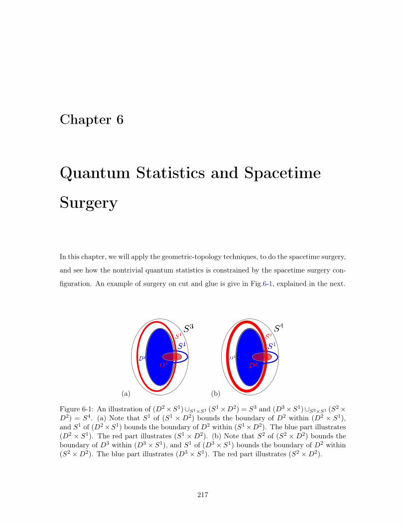
Chapter 6
Quantum Statistics and Spacetime
Surgery
In this chapter, we will apply the geometric-topology techniques, to do the spacetime surgery,
and see how the nontrivial quantum statistics is constrained by the spacetime surgery con-
figuration. An example of surgery on cut and glue is give in Fig.6-1, explained in the next.
(a) (b)
Figure 6-1: An illustration of (𝐷2×𝑆1)∪𝑆1×𝑆1 (𝑆1×𝐷2) = 𝑆3 and (𝐷3×𝑆1)∪𝑆2×𝑆1 (𝑆2×𝐷2) = 𝑆4. (a) Note that 𝑆1 of (𝑆1 × 𝐷2) bounds the boundary of 𝐷2 within (𝐷2 × 𝑆1),and 𝑆1 of (𝐷2×𝑆1) bounds the boundary of 𝐷2 within (𝑆1×𝐷2). The blue part illustrates(𝐷2 × 𝑆1). The red part illustrates (𝑆1 ×𝐷2). (b) Note that 𝑆2 of (𝑆2 ×𝐷2) bounds theboundary of 𝐷3 within (𝐷3 × 𝑆1), and 𝑆1 of (𝐷3 × 𝑆1) bounds the boundary of 𝐷2 within(𝑆2 ×𝐷2). The blue part illustrates (𝐷3 × 𝑆1). The red part illustrates (𝑆2 ×𝐷2).
217
6.1 Some properties of the spacetime surgery from geometric-
topology
We will discuss the surgery on cutting and gluing of 𝑑-manifold ℳ𝑑. We denote that 𝑆𝑑 is
a 𝑑-sphere, 𝐷𝑑 is a 𝑑-ball or called a 𝑑-disk, 𝑇 𝑑 is a 𝑑-torus. The notation for gluing the
boundaries of two manifoldsℳ1 andℳ2 is:
ℳ1 ∪𝐵;𝜙ℳ2. (6.1)
It requires that the boundary ofℳ1 andℳ2 are the same. Namely,
𝜕ℳ1 = −𝜕ℳ2 = 𝐵. (6.2)
We have a extra mapping 𝜙 allowed by diffeomorphism when gluing two manifolds. In
particular, we will focus on a 𝜙 of mapping class group (MCG) in our work. Thus, we can
apply any element of 𝜙 ∈ MCG(𝐵). For 𝜙 = 1 as a trivial identity map, we may simply
denoteℳ1 ∪𝐵ℳ2 =ℳ1 ∪𝐵,𝐼ℳ2.
The connected sum of two 𝑑-dimensional manifoldsℳ1 anℳ2 is denoted as
ℳ1#ℳ2. (6.3)
Say, we cut a ball 𝐷𝑑 (𝐷 for the disk 𝐷𝑑 or the same a ball 𝐵 for the 𝐵𝑑) out of the ℳ1
and ℳ2. Each of the complement space defined as ℳ1r𝐷𝑑 and ℳ2r𝐷𝑑 has a boundary
of a sphere 𝑆𝑑−1. We glue the two manifoldsℳ1 andℳ2 by a cylinder 𝑆𝑑−1× 𝐼 where the
𝐼 is a 1 dimensional interval.
The list of simple (non-exotic) 3-manifolds and 4-manifolds we will focus on those without
boundaries and those with boundaries. Also another list of 2-manifolds (as the boundaries
of 3-manifolds) and 3-manifolds (as the boundaries of 4-manifolds), all are summarized in
Table 6.1.
218
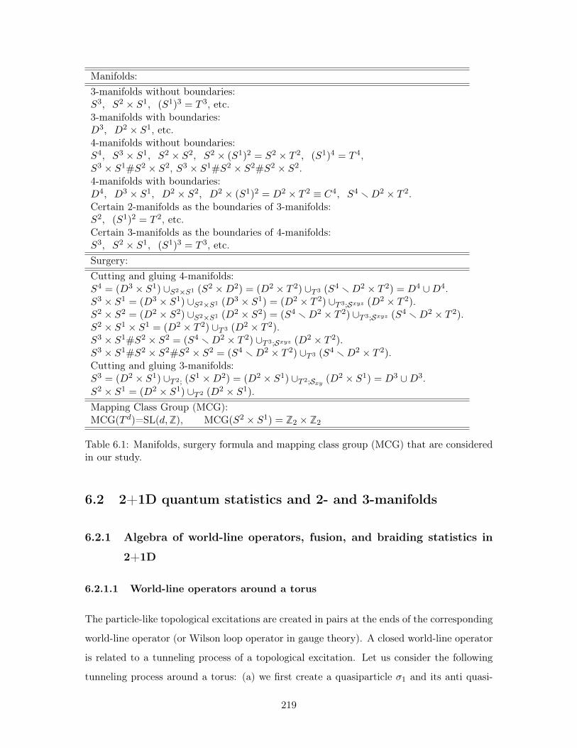
Manifolds:3-manifolds without boundaries:𝑆3, 𝑆2 × 𝑆1, (𝑆1)3 = 𝑇 3, etc.3-manifolds with boundaries:𝐷3, 𝐷2 × 𝑆1, etc.4-manifolds without boundaries:𝑆4, 𝑆3 × 𝑆1, 𝑆2 × 𝑆2, 𝑆2 × (𝑆1)2 = 𝑆2 × 𝑇 2, (𝑆1)4 = 𝑇 4,𝑆3 × 𝑆1#𝑆2 × 𝑆2, 𝑆3 × 𝑆1#𝑆2 × 𝑆2#𝑆2 × 𝑆2.4-manifolds with boundaries:𝐷4, 𝐷3 × 𝑆1, 𝐷2 × 𝑆2, 𝐷2 × (𝑆1)2 = 𝐷2 × 𝑇 2 ≡ 𝐶4, 𝑆4 r𝐷2 × 𝑇 2.Certain 2-manifolds as the boundaries of 3-manifolds:𝑆2, (𝑆1)2 = 𝑇 2, etc.Certain 3-manifolds as the boundaries of 4-manifolds:𝑆3, 𝑆2 × 𝑆1, (𝑆1)3 = 𝑇 3, etc.Surgery:Cutting and gluing 4-manifolds:𝑆4 = (𝐷3 × 𝑆1) ∪𝑆2×𝑆1 (𝑆2 ×𝐷2) = (𝐷2 × 𝑇 2) ∪𝑇 3 (𝑆4 r𝐷2 × 𝑇 2) = 𝐷4 ∪𝐷4.𝑆3 × 𝑆1 = (𝐷3 × 𝑆1) ∪𝑆2×𝑆1 (𝐷3 × 𝑆1) = (𝐷2 × 𝑇 2) ∪𝑇 3;𝒮𝑥𝑦𝑧 (𝐷2 × 𝑇 2).𝑆2 × 𝑆2 = (𝐷2 × 𝑆2) ∪𝑆2×𝑆1 (𝐷2 × 𝑆2) = (𝑆4 r𝐷2 × 𝑇 2) ∪𝑇 3;𝒮𝑥𝑦𝑧 (𝑆4 r𝐷2 × 𝑇 2).𝑆2 × 𝑆1 × 𝑆1 = (𝐷2 × 𝑇 2) ∪𝑇 3 (𝐷2 × 𝑇 2).𝑆3 × 𝑆1#𝑆2 × 𝑆2 = (𝑆4 r𝐷2 × 𝑇 2) ∪𝑇 3;𝒮𝑥𝑦𝑧 (𝐷2 × 𝑇 2).𝑆3 × 𝑆1#𝑆2 × 𝑆2#𝑆2 × 𝑆2 = (𝑆4 r𝐷2 × 𝑇 2) ∪𝑇 3 (𝑆4 r𝐷2 × 𝑇 2).Cutting and gluing 3-manifolds:𝑆3 = (𝐷2 × 𝑆1) ∪𝑇 2; (𝑆
1 ×𝐷2) = (𝐷2 × 𝑆1) ∪𝑇 2;𝒮𝑥𝑦(𝐷2 × 𝑆1) = 𝐷3 ∪𝐷3.
𝑆2 × 𝑆1 = (𝐷2 × 𝑆1) ∪𝑇 2 (𝐷2 × 𝑆1).Mapping Class Group (MCG):MCG(𝑇 𝑑)=SL(𝑑,Z), MCG(𝑆2 × 𝑆1) = Z2 × Z2
Table 6.1: Manifolds, surgery formula and mapping class group (MCG) that are consideredin our study.
6.2 2+1D quantum statistics and 2- and 3-manifolds
6.2.1 Algebra of world-line operators, fusion, and braiding statistics in
2+1D
6.2.1.1 World-line operators around a torus
The particle-like topological excitations are created in pairs at the ends of the corresponding
world-line operator (or Wilson loop operator in gauge theory). A closed world-line operator
is related to a tunneling process of a topological excitation. Let us consider the following
tunneling process around a torus: (a) we first create a quasiparticle 𝜎1 and its anti quasi-
219
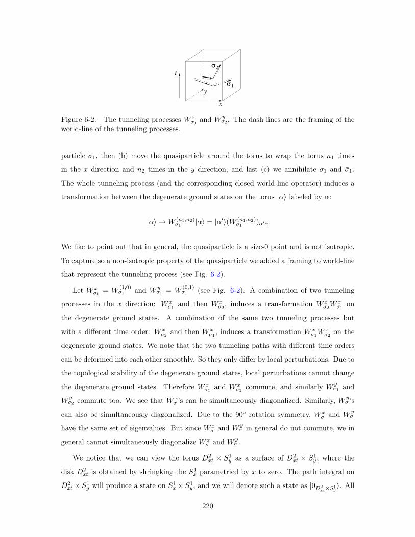
y
x
1
2
t
σ
σ
Figure 6-2: The tunneling processes 𝑊 𝑥𝜎1 and 𝑊 𝑦
𝜎2 . The dash lines are the framing of theworld-line of the tunneling processes.
particle ��1, then (b) move the quasiparticle around the torus to wrap the torus 𝑛1 times
in the 𝑥 direction and 𝑛2 times in the 𝑦 direction, and last (c) we annihilate 𝜎1 and ��1.
The whole tunneling process (and the corresponding closed world-line operator) induces a
transformation between the degenerate ground states on the torus |𝛼⟩ labeled by 𝛼:
|𝛼⟩ →𝑊 (𝑛1,𝑛2)𝜎1 |𝛼⟩ = |𝛼′⟩(𝑊 (𝑛1,𝑛2)
𝜎1 )𝛼′𝛼
We like to point out that in general, the quasiparticle is a size-0 point and is not isotropic.
To capture so a non-isotropic property of the quasiparticle we added a framing to world-line
that represent the tunneling process (see Fig. 6-2).
Let 𝑊 𝑥𝜎1 = 𝑊
(1,0)𝜎1 and 𝑊 𝑦
𝜎1 = 𝑊(0,1)𝜎1 (see Fig. 6-2). A combination of two tunneling
processes in the 𝑥 direction: 𝑊 𝑥𝜎1 and then 𝑊 𝑥
𝜎2 , induces a transformation 𝑊 𝑥𝜎2𝑊
𝑥𝜎1 on
the degenerate ground states. A combination of the same two tunneling processes but
with a different time order: 𝑊 𝑥𝜎2 and then 𝑊 𝑥
𝜎1 , induces a transformation 𝑊 𝑥𝜎1𝑊
𝑥𝜎2 on the
degenerate ground states. We note that the two tunneling paths with different time orders
can be deformed into each other smoothly. So they only differ by local perturbations. Due to
the topological stability of the degenerate ground states, local perturbations cannot change
the degenerate ground states. Therefore 𝑊 𝑥𝜎1 and 𝑊 𝑥
𝜎2 commute, and similarly 𝑊 𝑦𝜎1 and
𝑊 𝑦𝜎2 commute too. We see that 𝑊 𝑥
𝜎 ’s can be simultaneously diagonalized. Similarly, 𝑊 𝑦𝜎 ’s
can also be simultaneously diagonalized. Due to the 90∘ rotation symmetry, 𝑊 𝑥𝜎 and 𝑊 𝑦
𝜎
have the same set of eigenvalues. But since 𝑊 𝑥𝜎 and 𝑊 𝑦
𝜎 in general do not commute, we in
general cannot simultaneously diagonalize 𝑊 𝑥𝜎 and 𝑊 𝑦
𝜎 .
We notice that we can view the torus 𝐷2𝑥𝑡 × 𝑆1
𝑦 as a surface of 𝐷2𝑥𝑡 × 𝑆1
𝑦 , where the
disk 𝐷2𝑥𝑡 is obtained by shringking the 𝑆1
𝑥 parametried by 𝑥 to zero. The path integral on
𝐷2𝑥𝑡 × 𝑆1
𝑦 will produce a state on 𝑆1𝑥 × 𝑆1
𝑦 , and we will denote such a state as |0𝐷2𝑥𝑡×𝑆1
𝑦⟩. All
220
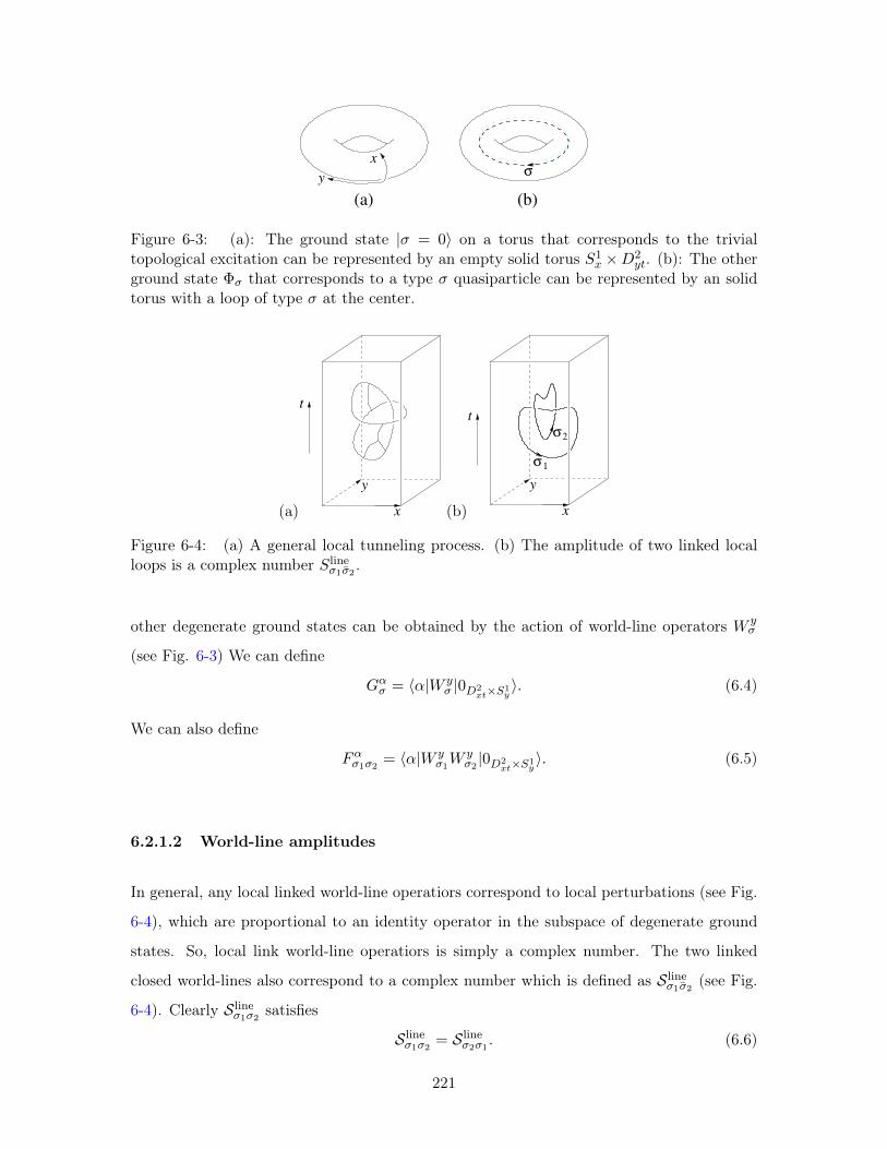
y
x
(b)
σ
(a)
Figure 6-3: (a): The ground state |𝜎 = 0⟩ on a torus that corresponds to the trivialtopological excitation can be represented by an empty solid torus 𝑆1
𝑥 ×𝐷2𝑦𝑡. (b): The other
ground state Φ𝜎 that corresponds to a type 𝜎 quasiparticle can be represented by an solidtorus with a loop of type 𝜎 at the center.
(a)
y
x
t
(b)(c)
x
y
t
σ2
σ1
Figure 6-4: (a) A general local tunneling process. (b) The amplitude of two linked localloops is a complex number 𝑆line
𝜎1��2 .
other degenerate ground states can be obtained by the action of world-line operators 𝑊 𝑦𝜎
(see Fig. 6-3) We can define
𝐺𝛼𝜎 = ⟨𝛼|𝑊 𝑦𝜎 |0𝐷2
𝑥𝑡×𝑆1𝑦⟩. (6.4)
We can also define
𝐹𝛼𝜎1𝜎2 = ⟨𝛼|𝑊 𝑦𝜎1𝑊
𝑦𝜎2 |0𝐷2
𝑥𝑡×𝑆1𝑦⟩. (6.5)
6.2.1.2 World-line amplitudes
In general, any local linked world-line operatiors correspond to local perturbations (see Fig.
6-4), which are proportional to an identity operator in the subspace of degenerate ground
states. So, local link world-line operatiors is simply a complex number. The two linked
closed world-lines also correspond to a complex number which is defined as 𝒮 line𝜎1��2 (see Fig.
6-4). Clearly 𝒮 line𝜎1𝜎2 satisfies
𝒮 line𝜎1𝜎2 = 𝒮 line
𝜎2𝜎1 . (6.6)
221
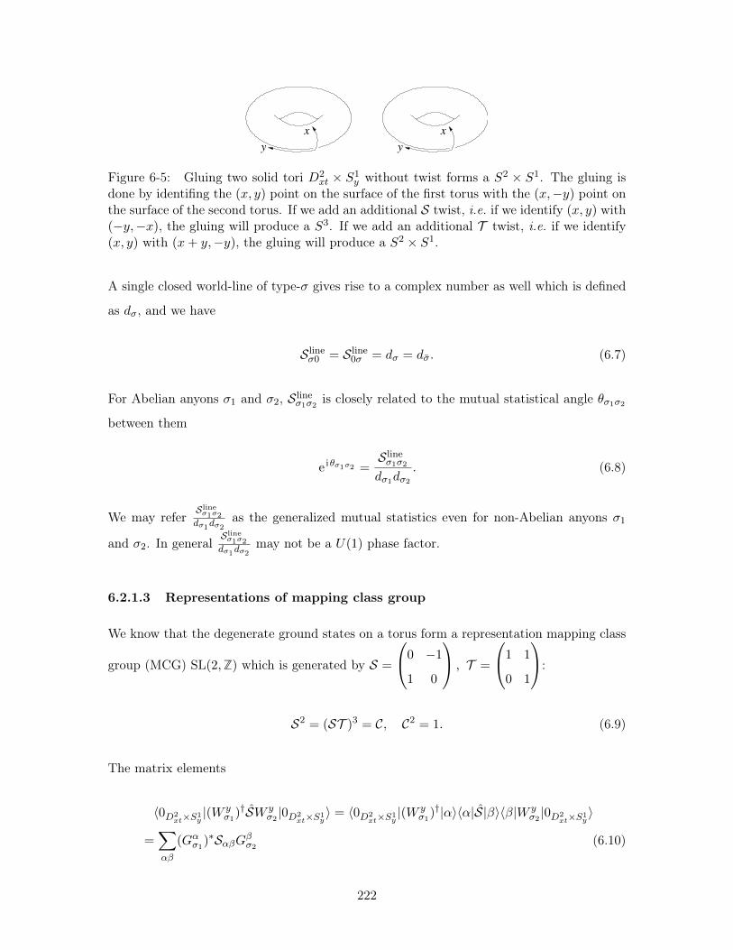
y
x
y
x
Figure 6-5: Gluing two solid tori 𝐷2𝑥𝑡 × 𝑆1
𝑦 without twist forms a 𝑆2 × 𝑆1. The gluing isdone by identifing the (𝑥, 𝑦) point on the surface of the first torus with the (𝑥,−𝑦) point onthe surface of the second torus. If we add an additional 𝒮 twist, i.e. if we identify (𝑥, 𝑦) with(−𝑦,−𝑥), the gluing will produce a 𝑆3. If we add an additional 𝒯 twist, i.e. if we identify(𝑥, 𝑦) with (𝑥+ 𝑦,−𝑦), the gluing will produce a 𝑆2 × 𝑆1.
A single closed world-line of type-𝜎 gives rise to a complex number as well which is defined
as 𝑑𝜎, and we have
𝒮 line𝜎0 = 𝒮 line
0𝜎 = 𝑑𝜎 = 𝑑��. (6.7)
For Abelian anyons 𝜎1 and 𝜎2, 𝒮 line𝜎1𝜎2 is closely related to the mutual statistical angle 𝜃𝜎1𝜎2
between them
e i𝜃𝜎1𝜎2 =𝒮 line𝜎1𝜎2
𝑑𝜎1𝑑𝜎2. (6.8)
We may refer𝒮line𝜎1𝜎2
𝑑𝜎1𝑑𝜎2as the generalized mutual statistics even for non-Abelian anyons 𝜎1
and 𝜎2. In general𝒮line𝜎1𝜎2
𝑑𝜎1𝑑𝜎2may not be a 𝑈(1) phase factor.
6.2.1.3 Representations of mapping class group
We know that the degenerate ground states on a torus form a representation mapping class
group (MCG) SL(2,Z) which is generated by 𝒮 =
⎛⎝0 −1
1 0
⎞⎠ , 𝒯 =
⎛⎝1 1
0 1
⎞⎠:
𝒮2 = (𝒮𝒯 )3 = 𝒞, 𝒞2 = 1. (6.9)
The matrix elements
⟨0𝐷2𝑥𝑡×𝑆1
𝑦|(𝑊 𝑦
𝜎1)†𝒮𝑊 𝑦
𝜎2 |0𝐷2𝑥𝑡×𝑆1
𝑦⟩ = ⟨0𝐷2
𝑥𝑡×𝑆1𝑦|(𝑊 𝑦
𝜎1)†|𝛼⟩⟨𝛼|𝒮|𝛽⟩⟨𝛽|𝑊 𝑦
𝜎2 |0𝐷2𝑥𝑡×𝑆1
𝑦⟩
=∑𝛼𝛽
(𝐺𝛼𝜎1)*𝒮𝛼𝛽𝐺𝛽𝜎2 (6.10)
222
can be computed via the path integral on two solid tori 𝐷2𝑥𝑡×𝑆1
𝑦 , one with a closed world-line
𝑊 𝑦𝜎1 at the center and the other with a closed world-line 𝑊 𝑦
𝜎2 at the center. The two solid
tori are glued along the surface 𝑆1𝑥 × 𝑆1
𝑦 but with a 𝒮 =
⎛⎝0 −1
1 0
⎞⎠ twist (𝑥, 𝑦) → (−𝑦, 𝑥)
(see Fig. 6-5). The resulting space-time is 𝑆3 = 𝐷2𝑥𝑡 × 𝑆1
𝑦 ∪𝐵;𝒮 𝐷2𝑥𝑡 × 𝑆1
𝑦 with two linked
closed world-lines 𝜎1 and 𝜎2 (see Fig. 6-4 which describes two linked closed world-lines).
Here 𝑀 ∪𝐵 𝑁 is the union of 𝑀 and 𝑁 alone the boundary 𝐵 = 𝜕𝑀 = −𝜕𝑁 .
Combined with the above discussion, we find that
𝑍
⎛⎝ 12
⎞⎠ =∑𝛼𝛽
(𝐺𝛼𝜎1)*𝒮𝛼𝛽𝐺𝛽𝜎2 = 𝒮 line
��1𝜎2𝑍(𝑆3)
= 𝒮 line��1𝜎2
∑𝛼𝛽
(𝐺𝛼0 )*𝒮𝛼𝛽𝐺𝛽0 , (6.11)
where 𝑍(𝑆3) is the partition function on 𝑆3, which happen to equal to∑
𝛼𝛽(𝐺𝛼0 )
*𝒮𝛼𝛽𝐺𝛽0 . We
obtain an important relation that connects the representation of MCG and the amplitudes
of local closed world-lines: ∑𝛼𝛽(𝐺
𝛼𝜎1)
*𝒮𝛼𝛽𝐺𝛽𝜎2∑𝛼𝛽(𝐺
𝛼0 )
*𝒮𝛼𝛽𝐺𝛽0= 𝒮 line
��1𝜎2 . (6.12)
Here 𝑆line��1𝜎2 is the amplitude of two linked world-line loops (see Fig. 6-4).
Next, let us consider the partition function on space-time that is formed by disconnected
three manifolds 𝑀 and 𝑁 , which denoted as 𝑀 ⊔𝑁 . We have
𝑍(𝑀 ⊔𝑁) = 𝑍(𝑀)𝑍(𝑁), (6.13)
for fixed-point partition function of topologically ordered state. We divide 𝑀 into two
pieces, 𝑀𝑈 and 𝑀𝐷: 𝑀 = 𝑀𝐷 ∪𝜕𝑀𝐷𝑀𝑈 . We also divide 𝑁 into two pieces, 𝑁𝑈 and 𝑀𝐷:
𝑁 = 𝑁𝐷 ∪𝜕𝑁𝐷𝑁𝑈 . If the boundary of 𝑀𝐷 and 𝑁𝐷 is the same configuration as the sphere
𝑆2 = 𝜕𝑀𝐷 = 𝜕𝑁𝐷 with the same defect configurations on 𝑆2, and if the ground state
degeneracy of this spatial configuration is unique (namely, the dimension of Hilbert space is
223
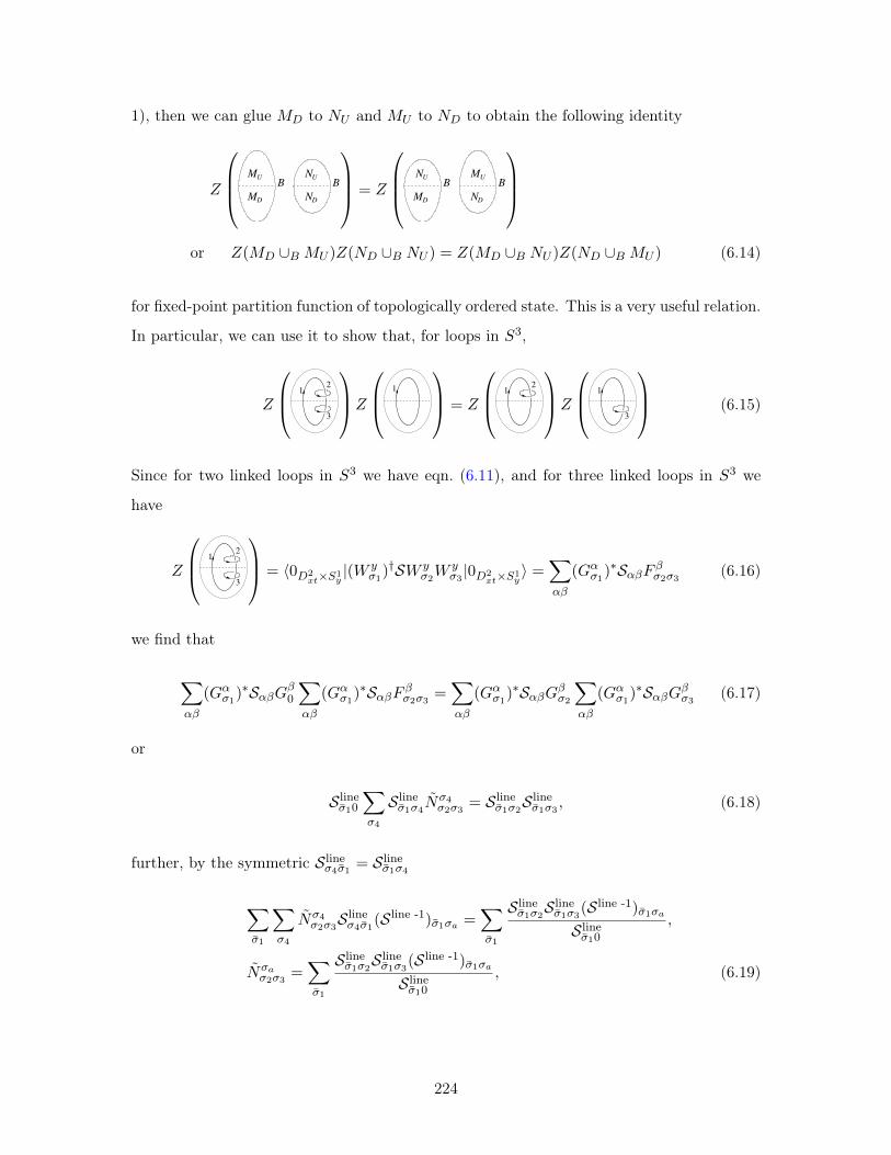
1), then we can glue 𝑀𝐷 to 𝑁𝑈 and 𝑀𝑈 to 𝑁𝐷 to obtain the following identity
𝑍
⎛⎜⎜⎝ M
U
D
B B
ND
NUM
⎞⎟⎟⎠ = 𝑍
⎛⎜⎜⎝ M
U
D
BN
BMU
ND
⎞⎟⎟⎠or 𝑍(𝑀𝐷 ∪𝐵 𝑀𝑈 )𝑍(𝑁𝐷 ∪𝐵 𝑁𝑈 ) = 𝑍(𝑀𝐷 ∪𝐵 𝑁𝑈 )𝑍(𝑁𝐷 ∪𝐵 𝑀𝑈 ) (6.14)
for fixed-point partition function of topologically ordered state. This is a very useful relation.
In particular, we can use it to show that, for loops in 𝑆3,
𝑍
⎛⎜⎝ 12
3
⎞⎟⎠𝑍
⎛⎜⎝ 1
⎞⎟⎠ = 𝑍
⎛⎜⎝ 12
⎞⎟⎠𝑍
⎛⎜⎝ 1
3
⎞⎟⎠ (6.15)
Since for two linked loops in 𝑆3 we have eqn. (6.11), and for three linked loops in 𝑆3 we
have
𝑍
⎛⎜⎝ 12
3
⎞⎟⎠ = ⟨0𝐷2𝑥𝑡×𝑆1
𝑦|(𝑊 𝑦
𝜎1)†𝒮𝑊 𝑦
𝜎2𝑊𝑦𝜎3 |0𝐷2
𝑥𝑡×𝑆1𝑦⟩ =
∑𝛼𝛽
(𝐺𝛼𝜎1)*𝒮𝛼𝛽𝐹 𝛽𝜎2𝜎3 (6.16)
we find that
∑𝛼𝛽
(𝐺𝛼𝜎1)*𝒮𝛼𝛽𝐺𝛽0
∑𝛼𝛽
(𝐺𝛼𝜎1)*𝒮𝛼𝛽𝐹 𝛽𝜎2𝜎3 =
∑𝛼𝛽
(𝐺𝛼𝜎1)*𝒮𝛼𝛽𝐺𝛽𝜎2
∑𝛼𝛽
(𝐺𝛼𝜎1)*𝒮𝛼𝛽𝐺𝛽𝜎3 (6.17)
or
𝒮 line��10
∑𝜎4
𝒮 line��1𝜎4��
𝜎4𝜎2𝜎3 = 𝒮 line
��1𝜎2𝒮line��1𝜎3 , (6.18)
further, by the symmetric 𝒮 line𝜎4��1 = 𝒮 line
��1𝜎4
∑��1
∑𝜎4
��𝜎4𝜎2𝜎3𝒮
line𝜎4��1(𝒮
line -1)��1𝜎𝑎 =∑��1
𝒮 line��1𝜎2𝒮
line��1𝜎3(𝒮
line -1)��1𝜎𝑎𝒮 line��10
,
��𝜎𝑎𝜎2𝜎3 =
∑��1
𝒮 line��1𝜎2𝒮
line��1𝜎3(𝒮
line -1)��1𝜎𝑎𝒮 line��10
, (6.19)
224
where
��𝜎4𝜎2𝜎3 =
∑𝛽
(𝐺−1)𝜎4𝛽 𝐹𝛽𝜎2𝜎3 . (6.20)
The above is the Verlinde formula. Compare to the usual: Verlinde formula
𝒩 𝑐𝑎𝑏 =
∑𝑚
𝒮𝑎𝑚𝒮𝑏𝑚𝒮𝑐𝑚𝒮1𝑚
∈ N. (6.21)
6.2.1.4 Canonical world-line operators and canonical basis
In general the norm of the state 𝑊 𝑦𝜎 |0𝐷2
𝑥𝑡×𝑆1𝑦⟩ is proportional to the length of the world-line
operator. We choose a normalization of the local operators that form the world-line properly,
so that
⟨0𝐷2𝑥𝑡×𝑆1
𝑦|(𝑊 𝑦
𝜎 )†𝑊 𝑦
𝜎 |0𝐷2𝑥𝑡×𝑆1
𝑦⟩
= ⟨0𝐷2𝑥𝑡×𝑆1
𝑦|𝑊 𝑦
��𝑊𝑦𝜎 |0𝐷2
𝑥𝑡×𝑆1𝑦⟩ (6.22)
is independent of the length and the shape of the world-line operator 𝑊 𝑦𝜎 . Here �� is the
anti-particle of 𝜎 and we have assumed that 𝑊 𝑦�� = (𝑊 𝑦
𝜎 )†. For such proper normalized
world-line operators, we conjecture that
⟨0𝐷2𝑥𝑡×𝑆1
𝑦|𝑊 𝑦
��𝑊𝑦𝜎 |0𝐷2
𝑥𝑡×𝑆1𝑦⟩ = 1, (6.23)
assuming ⟨0𝐷2𝑥𝑡×𝑆1
𝑦|0𝐷2
𝑥𝑡×𝑆1𝑦⟩ = 1. In this case, 𝐺𝛼𝜎 = 𝛿𝛼𝜎, and 𝐹𝛼𝜎1𝜎2 = ��𝛼
𝜎1𝜎2 = 𝑁𝛼𝜎1𝜎2 , where
𝑁𝜎3𝜎1𝜎2 are integers which describe the fusion of two topological excitations via the following
fusion algebra
𝜎1𝜎2 = 𝑁𝜎3𝜎2𝜎1𝜎3. (6.24)
To see the relation 𝐹 𝜎3𝜎1𝜎2 = ��𝜎3𝜎1𝜎2 = 𝑁𝜎3
𝜎1𝜎2 , we note that
𝐹 𝜎3𝜎1𝜎2 = ⟨0𝐷2𝑥𝑡×𝑆1
𝑦|𝑊 𝑦
��3𝑊𝑦𝜎1𝑊
𝑦𝜎2 |0𝐷2
𝑥𝑡×𝑆1𝑦⟩. (6.25)
The above can be viewed as a path integral on 𝑆2 × 𝑆1 with three world-lines 𝜎1, 𝜎2, ��3
225
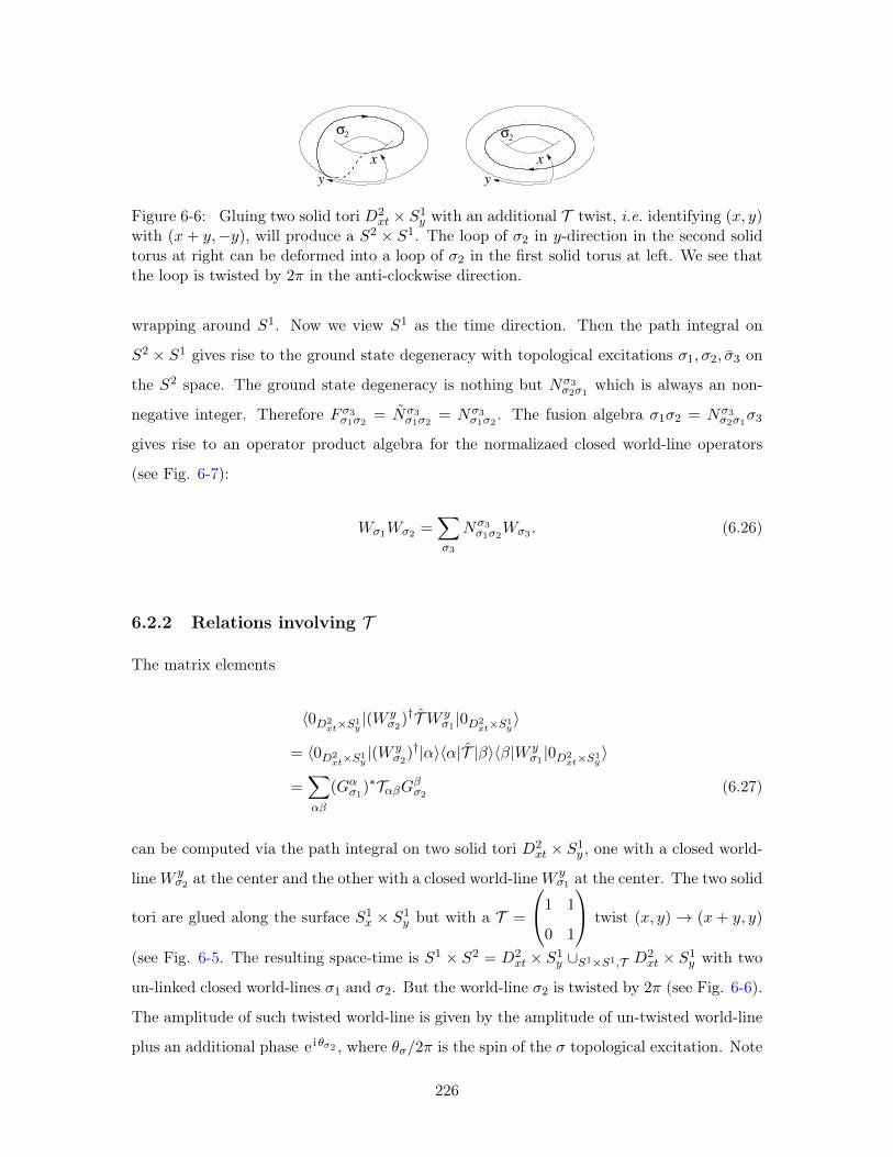
y
x
y
x
σ2σ2
Figure 6-6: Gluing two solid tori 𝐷2𝑥𝑡 × 𝑆1
𝑦 with an additional 𝒯 twist, i.e. identifying (𝑥, 𝑦)with (𝑥+ 𝑦,−𝑦), will produce a 𝑆2 × 𝑆1. The loop of 𝜎2 in 𝑦-direction in the second solidtorus at right can be deformed into a loop of 𝜎2 in the first solid torus at left. We see thatthe loop is twisted by 2𝜋 in the anti-clockwise direction.
wrapping around 𝑆1. Now we view 𝑆1 as the time direction. Then the path integral on
𝑆2 × 𝑆1 gives rise to the ground state degeneracy with topological excitations 𝜎1, 𝜎2, ��3 on
the 𝑆2 space. The ground state degeneracy is nothing but 𝑁𝜎3𝜎2𝜎1 which is always an non-
negative integer. Therefore 𝐹 𝜎3𝜎1𝜎2 = ��𝜎3𝜎1𝜎2 = 𝑁𝜎3
𝜎1𝜎2 . The fusion algebra 𝜎1𝜎2 = 𝑁𝜎3𝜎2𝜎1𝜎3
gives rise to an operator product algebra for the normalizaed closed world-line operators
(see Fig. 6-7):
𝑊𝜎1𝑊𝜎2 =∑𝜎3
𝑁𝜎3𝜎1𝜎2𝑊𝜎3 . (6.26)
6.2.2 Relations involving 𝒯
The matrix elements
⟨0𝐷2𝑥𝑡×𝑆1
𝑦|(𝑊 𝑦
𝜎2)†𝒯𝑊 𝑦
𝜎1 |0𝐷2𝑥𝑡×𝑆1
𝑦⟩
= ⟨0𝐷2𝑥𝑡×𝑆1
𝑦|(𝑊 𝑦
𝜎2)†|𝛼⟩⟨𝛼|𝒯 |𝛽⟩⟨𝛽|𝑊 𝑦
𝜎1 |0𝐷2𝑥𝑡×𝑆1
𝑦⟩
=∑𝛼𝛽
(𝐺𝛼𝜎1)*𝒯𝛼𝛽𝐺𝛽𝜎2 (6.27)
can be computed via the path integral on two solid tori 𝐷2𝑥𝑡 × 𝑆1
𝑦 , one with a closed world-
line𝑊 𝑦𝜎2 at the center and the other with a closed world-line𝑊 𝑦
𝜎1 at the center. The two solid
tori are glued along the surface 𝑆1𝑥 × 𝑆1
𝑦 but with a 𝒯 =
⎛⎝1 1
0 1
⎞⎠ twist (𝑥, 𝑦) → (𝑥 + 𝑦, 𝑦)
(see Fig. 6-5. The resulting space-time is 𝑆1 × 𝑆2 = 𝐷2𝑥𝑡 × 𝑆1
𝑦 ∪𝑆1×𝑆1,𝒯 𝐷2𝑥𝑡 × 𝑆1
𝑦 with two
un-linked closed world-lines 𝜎1 and 𝜎2. But the world-line 𝜎2 is twisted by 2𝜋 (see Fig. 6-6).
The amplitude of such twisted world-line is given by the amplitude of un-twisted world-line
plus an additional phase e i𝜃𝜎2 , where 𝜃𝜎/2𝜋 is the spin of the 𝜎 topological excitation. Note
226
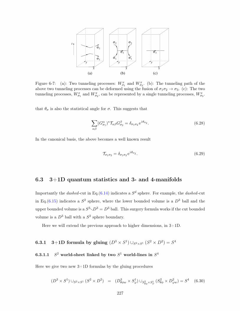
(a) (b) (c)
x
y y
x x
y
t
1
2
3 3
2
1
σ
σ
σ σ
σ
σ
σ1
2
σ
Figure 6-7: (a): Two tunneling processes: 𝑊 𝑥𝜎1 and 𝑊 𝑥
𝜎2 . (b): The tunneling path of theabove two tunneling processes can be deformed using the fusion of 𝜎1𝜎2 → 𝜎3. (c): The twotunneling processes, 𝑊 𝑥
𝜎1 and 𝑊 𝑥𝜎2 , can be represented by a single tunneling processes, 𝑊 𝑥
𝜎3 .
that 𝜃𝜎 is also the statistical angle for 𝜎. This suggests that
∑𝛼𝛽
(𝐺𝛼𝜎1)*𝒯𝛼𝛽𝐺𝛽𝜎2 = 𝛿𝜎1𝜎2 e
i𝜃𝜎2 . (6.28)
In the canonical basis, the above becomes a well known result
𝒯𝜎1𝜎2 = 𝛿𝜎1𝜎2 ei𝜃𝜎2 . (6.29)
6.3 3+1D quantum statistics and 3- and 4-manifolds
Importantly the dashed -cut in Eq.(6.14) indicates a 𝑆𝑑 sphere. For example, the dashed -cut
in Eq.(6.15) indicates a 𝑆2 sphere, where the lower bounded volume is a 𝐷3 ball and the
upper bounded volume is a 𝑆3r𝐷3 = 𝐷3 ball. This surgery formula works if the cut bounded
volume is a 𝐷3 ball with a 𝑆2 sphere boundary.
Here we will extend the previous approach to higher dimensions, in 3+1D.
6.3.1 3+1D formula by gluing (𝐷3 × 𝑆1) ∪𝑆2×𝑆1 (𝑆2 ×𝐷2) = 𝑆4
6.3.1.1 𝑆2 world-sheet linked by two 𝑆1 world-lines in 𝑆4
Here we give two new 3+1D formulas by the gluing procedures
(𝐷3 × 𝑆1) ∪𝑆2×𝑆1 (𝑆2 ×𝐷2) = (𝐷3𝜃𝜑𝑤 × 𝑆1
𝜙) ∪𝑆2𝜃𝜑×𝑆1
𝜙(𝑆2𝜃𝜑 ×𝐷2
𝜙𝑤) = 𝑆4 (6.30)
227
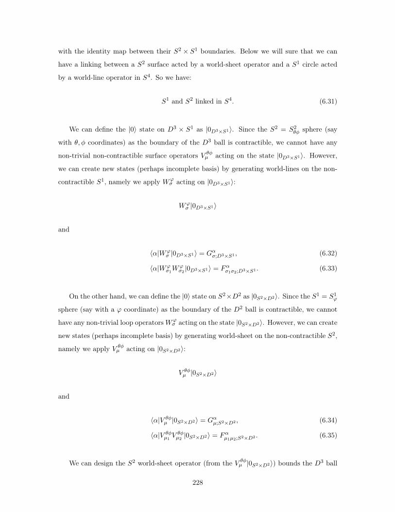
with the identity map between their 𝑆2 × 𝑆1 boundaries. Below we will sure that we can
have a linking between a 𝑆2 surface acted by a world-sheet operator and a 𝑆1 circle acted
by a world-line operator in 𝑆4. So we have:
𝑆1 and 𝑆2 linked in 𝑆4. (6.31)
We can define the |0⟩ state on 𝐷3 × 𝑆1 as |0𝐷3×𝑆1⟩. Since the 𝑆2 = 𝑆2𝜃𝜑 sphere (say
with 𝜃, 𝜑 coordinates) as the boundary of the 𝐷3 ball is contractible, we cannot have any
non-trivial non-contractible surface operators 𝑉 𝜃𝜑𝜇 acting on the state |0𝐷3×𝑆1⟩. However,
we can create new states (perhaps incomplete basis) by generating world-lines on the non-
contractible 𝑆1, namely we apply 𝑊𝜙𝜎 acting on |0𝐷3×𝑆1⟩:
𝑊𝜙𝜎 |0𝐷3×𝑆1⟩
and
⟨𝛼|𝑊𝜙𝜎 |0𝐷3×𝑆1⟩ = 𝐺𝛼𝜎;𝐷3×𝑆1 , (6.32)
⟨𝛼|𝑊𝜙𝜎1𝑊
𝜙𝜎2 |0𝐷3×𝑆1⟩ = 𝐹𝛼𝜎1𝜎2;𝐷3×𝑆1 . (6.33)
On the other hand, we can define the |0⟩ state on 𝑆2×𝐷2 as |0𝑆2×𝐷2⟩. Since the 𝑆1 = 𝑆1𝜙
sphere (say with a 𝜙 coordinate) as the boundary of the 𝐷2 ball is contractible, we cannot
have any non-trivial loop operators𝑊𝜙𝜎 acting on the state |0𝑆2×𝐷2⟩. However, we can create
new states (perhaps incomplete basis) by generating world-sheet on the non-contractible 𝑆2,
namely we apply 𝑉 𝜃𝜑𝜇 acting on |0𝑆2×𝐷2⟩:
𝑉 𝜃𝜑𝜇 |0𝑆2×𝐷2⟩
and
⟨𝛼|𝑉 𝜃𝜑𝜇 |0𝑆2×𝐷2⟩ = 𝐺𝛼𝜇;𝑆2×𝐷2 , (6.34)
⟨𝛼|𝑉 𝜃𝜑𝜇1 𝑉
𝜃𝜑𝜇2 |0𝑆2×𝐷2⟩ = 𝐹𝛼𝜇1𝜇2;𝑆2×𝐷2 . (6.35)
We can design the 𝑆2 world-sheet operator (from the 𝑉 𝜃𝜑𝜇 |0𝑆2×𝐷2⟩) bounds the 𝐷3 ball
228
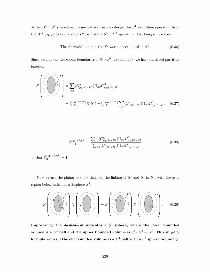
of the 𝐷3 × 𝑆1 spacetime, meanwhile we can also design the 𝑆1 world-line operator (from
the 𝑊𝜙𝜎 |0𝐷3×𝑆1⟩) bounds the 𝐷2 ball of the 𝑆2 ×𝐷2 spacetime. By doing so, we have:
The 𝑆1 world-line and the 𝑆2 world-sheet linked in 𝑆4. (6.36)
Since we glue the two copies boundaries of 𝑆2×𝑆1 via the map I, we have the glued partition
function:
𝑍
⎛⎜⎜⎜⎜⎜⎝
⎞⎟⎟⎟⎟⎟⎠ =∑𝛼𝛽
(𝐺𝛼𝜇1;𝑆2×𝐷2)*I𝛼𝛽𝐺
𝛽𝜎2;𝐷3×𝑆1
= ILink(𝑆2,𝑆1)𝜇1𝜎2 𝑍(𝑆4) = ILink(𝑆2,𝑆1)
𝜇1𝜎2
∑𝛼𝛽
(𝐺𝛼0;𝑆2×𝐷2)*I𝛼𝛽𝐺
𝛽0;𝐷3×𝑆1 , (6.37)
ILink(𝑆2,𝑆1)𝜇1𝜎2 =
∑𝛼𝛽(𝐺
𝛼𝜇1;𝑆2×𝐷2)
*I𝛼𝛽𝐺𝛽𝜎2;𝐷3×𝑆1∑
𝛼𝛽(𝐺𝛼0;𝑆2×𝐷2)*I𝛼𝛽𝐺
𝛽0;𝐷3×𝑆1
(6.38)
so that ILink(𝑆2,𝑆1)00 = 1.
Now we use the gluing to show that, for the linking of 𝑆2 and 𝑆1 in 𝑆4, with the gray
region below indicates a 2-sphere 𝑆2.
𝑍
⎛⎜⎜⎜⎜⎜⎝1
2
3
⎞⎟⎟⎟⎟⎟⎠𝑍
⎛⎜⎜⎜⎜⎜⎝1
⎞⎟⎟⎟⎟⎟⎠ = 𝑍
⎛⎜⎜⎜⎜⎜⎝1
2
⎞⎟⎟⎟⎟⎟⎠𝑍
⎛⎜⎜⎜⎜⎜⎝1
3
⎞⎟⎟⎟⎟⎟⎠ . (6.39)
Importantly the dashed-cut indicates a 𝑆3 sphere, where the lower bounded
volume is a 𝐷4 ball and the upper bounded volume is 𝑆4r𝐷4 = 𝐷4. This surgery
formula works if the cut bounded volume is a 𝐷4 ball with a 𝑆3 sphere boundary.
229
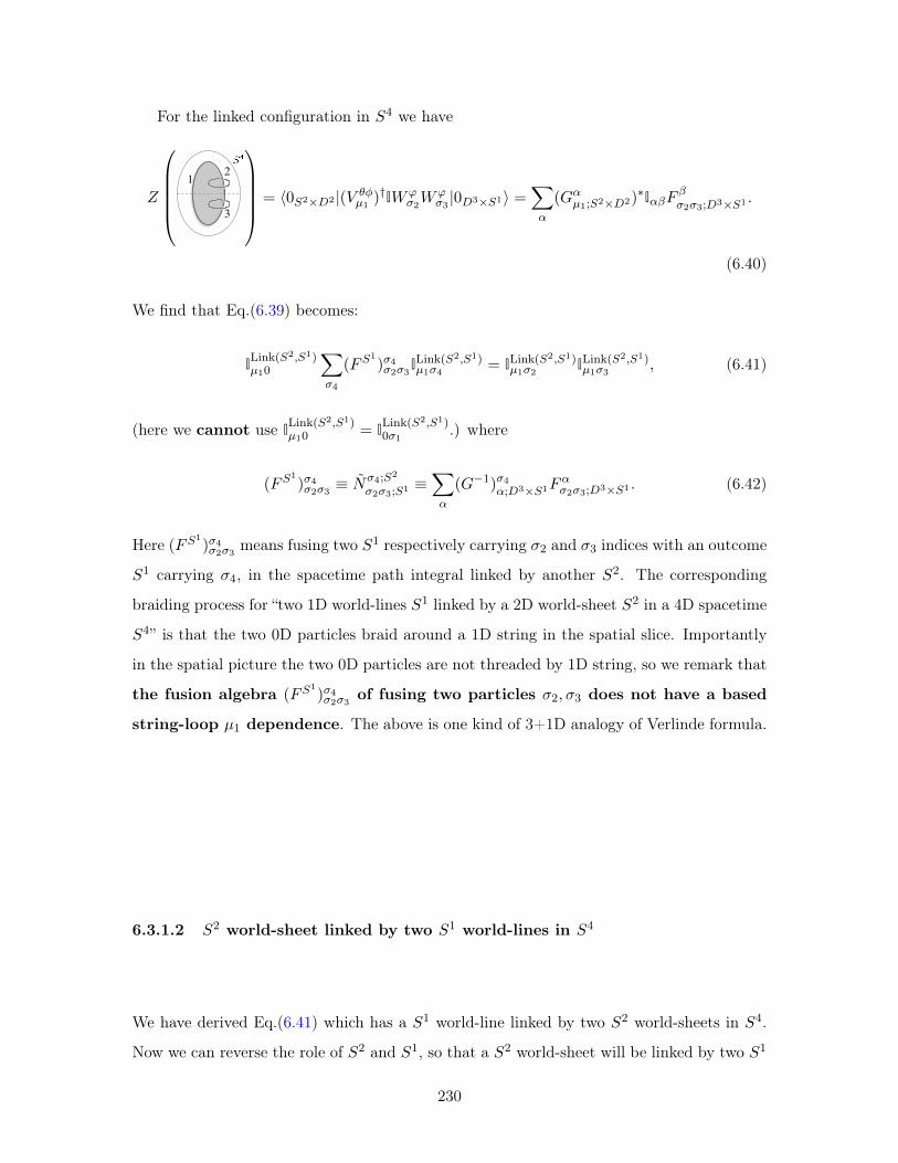
For the linked configuration in 𝑆4 we have
𝑍
⎛⎜⎜⎜⎜⎝1
2
3
⎞⎟⎟⎟⎟⎠ = ⟨0𝑆2×𝐷2 |(𝑉 𝜃𝜑𝜇1 )
†I𝑊𝜙𝜎2𝑊
𝜙𝜎3 |0𝐷3×𝑆1⟩ =
∑𝛼
(𝐺𝛼𝜇1;𝑆2×𝐷2)*I𝛼𝛽𝐹
𝛽𝜎2𝜎3;𝐷3×𝑆1 .
(6.40)
We find that Eq.(6.39) becomes:
ILink(𝑆2,𝑆1)𝜇10
∑𝜎4
(𝐹𝑆1)𝜎4𝜎2𝜎3ILink(𝑆2,𝑆1)
𝜇1𝜎4 = ILink(𝑆2,𝑆1)𝜇1𝜎2 ILink(𝑆2,𝑆1)
𝜇1𝜎3 , (6.41)
(here we cannot use ILink(𝑆2,𝑆1)𝜇10
= ILink(𝑆2,𝑆1)0𝜎1
.) where
(𝐹𝑆1)𝜎4𝜎2𝜎3 ≡ ��
𝜎4;𝑆2
𝜎2𝜎3;𝑆1 ≡∑𝛼
(𝐺−1)𝜎4𝛼;𝐷3×𝑆1𝐹
𝛼𝜎2𝜎3;𝐷3×𝑆1 . (6.42)
Here (𝐹𝑆1)𝜎4𝜎2𝜎3 means fusing two 𝑆1 respectively carrying 𝜎2 and 𝜎3 indices with an outcome
𝑆1 carrying 𝜎4, in the spacetime path integral linked by another 𝑆2. The corresponding
braiding process for “two 1D world-lines 𝑆1 linked by a 2D world-sheet 𝑆2 in a 4D spacetime
𝑆4” is that the two 0D particles braid around a 1D string in the spatial slice. Importantly
in the spatial picture the two 0D particles are not threaded by 1D string, so we remark that
the fusion algebra (𝐹𝑆1)𝜎4𝜎2𝜎3 of fusing two particles 𝜎2, 𝜎3 does not have a based
string-loop 𝜇1 dependence. The above is one kind of 3+1D analogy of Verlinde formula.
6.3.1.2 𝑆2 world-sheet linked by two 𝑆1 world-lines in 𝑆4
We have derived Eq.(6.41) which has a 𝑆1 world-line linked by two 𝑆2 world-sheets in 𝑆4.
Now we can reverse the role of 𝑆2 and 𝑆1, so that a 𝑆2 world-sheet will be linked by two 𝑆1
230
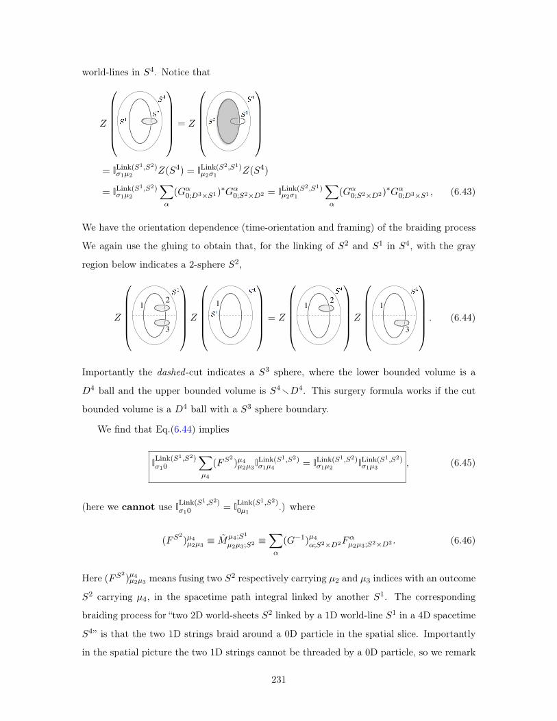
world-lines in 𝑆4. Notice that
𝑍
⎛⎜⎜⎜⎜⎜⎝
⎞⎟⎟⎟⎟⎟⎠ = 𝑍
⎛⎜⎜⎜⎜⎜⎝
⎞⎟⎟⎟⎟⎟⎠= ILink(𝑆1,𝑆2)
𝜎1𝜇2 𝑍(𝑆4) = ILink(𝑆2,𝑆1)𝜇2𝜎1 𝑍(𝑆4)
= ILink(𝑆1,𝑆2)𝜎1𝜇2
∑𝛼
(𝐺𝛼0;𝐷3×𝑆1)*𝐺𝛼0;𝑆2×𝐷2 = ILink(𝑆2,𝑆1)
𝜇2𝜎1
∑𝛼
(𝐺𝛼0;𝑆2×𝐷2)*𝐺𝛼0;𝐷3×𝑆1 , (6.43)
We have the orientation dependence (time-orientation and framing) of the braiding process
We again use the gluing to obtain that, for the linking of 𝑆2 and 𝑆1 in 𝑆4, with the gray
region below indicates a 2-sphere 𝑆2,
𝑍
⎛⎜⎜⎜⎜⎜⎝1
2
3
⎞⎟⎟⎟⎟⎟⎠𝑍
⎛⎜⎜⎜⎜⎜⎝1
⎞⎟⎟⎟⎟⎟⎠ = 𝑍
⎛⎜⎜⎜⎜⎜⎝1
2
⎞⎟⎟⎟⎟⎟⎠𝑍
⎛⎜⎜⎜⎜⎜⎝1
3
⎞⎟⎟⎟⎟⎟⎠ . (6.44)
Importantly the dashed -cut indicates a 𝑆3 sphere, where the lower bounded volume is a
𝐷4 ball and the upper bounded volume is 𝑆4r𝐷4. This surgery formula works if the cut
bounded volume is a 𝐷4 ball with a 𝑆3 sphere boundary.
We find that Eq.(6.44) implies
ILink(𝑆1,𝑆2)𝜎10
∑𝜇4
(𝐹𝑆2)𝜇4𝜇2𝜇3ILink(𝑆1,𝑆2)
𝜎1𝜇4 = ILink(𝑆1,𝑆2)𝜎1𝜇2 ILink(𝑆1,𝑆2)
𝜎1𝜇3 , (6.45)
(here we cannot use ILink(𝑆1,𝑆2)𝜎10
= ILink(𝑆1,𝑆2)0𝜇1
.) where
(𝐹𝑆2)𝜇4𝜇2𝜇3 ≡ ��
𝜇4;𝑆1
𝜇2𝜇3;𝑆2 ≡∑𝛼
(𝐺−1)𝜇4𝛼;𝑆2×𝐷2𝐹
𝛼𝜇2𝜇3;𝑆2×𝐷2 . (6.46)
Here (𝐹𝑆2)𝜇4𝜇2𝜇3 means fusing two 𝑆2 respectively carrying 𝜇2 and 𝜇3 indices with an outcome
𝑆2 carrying 𝜇4, in the spacetime path integral linked by another 𝑆1. The corresponding
braiding process for “two 2D world-sheets 𝑆2 linked by a 1D world-line 𝑆1 in a 4D spacetime
𝑆4” is that the two 1D strings braid around a 0D particle in the spatial slice. Importantly
in the spatial picture the two 1D strings cannot be threaded by a 0D particle, so we remark
231
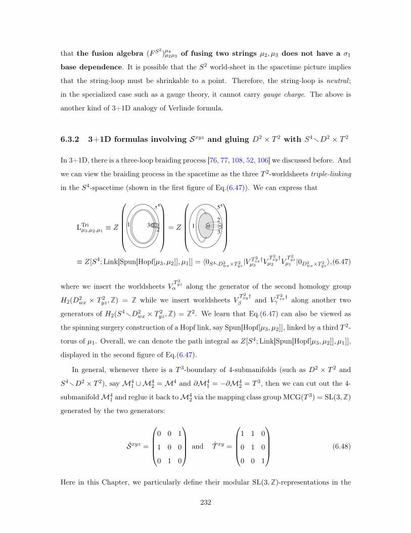
that the fusion algebra (𝐹𝑆2)𝜇4𝜇2𝜇3 of fusing two strings 𝜇2, 𝜇3 does not have a 𝜎1
base dependence. It is possible that the 𝑆2 world-sheet in the spacetime picture implies
that the string-loop must be shrinkable to a point. Therefore, the string-loop is neutral ;
in the specialized case such as a gauge theory, it cannot carry gauge charge. The above is
another kind of 3+1D analogy of Verlinde formula.
6.3.2 3+1D formulas involving 𝒮𝑥𝑦𝑧 and gluing 𝐷2 × 𝑇 2 with 𝑆4r𝐷2 × 𝑇 2
In 3+1D, there is a three-loop braiding process [76, 77, 108, 52, 106] we discussed before. And
we can view the braiding process in the spacetime as the three 𝑇 2-worldsheets triple-linking
in the 𝑆4-spacetime (shown in the first figure of Eq.(6.47)). We can express that
LTri𝜇3,𝜇2,𝜇1 ≡ 𝑍
⎛⎜⎜⎜⎜⎜⎝12
3
⎞⎟⎟⎟⎟⎟⎠ = 𝑍
⎛⎜⎜⎜⎜⎜⎝ 12
3
⎞⎟⎟⎟⎟⎟⎠≡ 𝑍[𝑆4;Link[Spun[Hopf[𝜇3, 𝜇2]], 𝜇1]] = ⟨0𝑆4r𝐷2
𝑤𝑥×𝑇 2𝑦𝑧|𝑉 𝑇 2
𝑧𝑥†𝜇3 𝑉
𝑇 2𝑥𝑦†
𝜇2 𝑉𝑇 2𝑦𝑧
𝜇1 |0𝐷2𝑤𝑥×𝑇 2
𝑦𝑧⟩,(6.47)
where we insert the worldsheets 𝑉𝑇 2𝑦𝑧
𝛼 along the generator of the second homology group
𝐻2(𝐷2𝑤𝑥 × 𝑇 2
𝑦𝑧,Z) = Z while we insert worldsheets 𝑉𝑇 2𝑥𝑦†
𝛽 and 𝑉𝑇 2𝑧𝑥†
𝛾 along another two
generators of 𝐻2(𝑆4r𝐷2
𝑤𝑥 × 𝑇 2𝑦𝑧,Z) = Z2. We learn that Eq.(6.47) can also be viewed as
the spinning surgery construction of a Hopf link, say Spun[Hopf[𝜇3, 𝜇2]], linked by a third 𝑇 2-
torus of 𝜇1. Overall, we can denote the path integral as 𝑍[𝑆4;Link[Spun[Hopf[𝜇3, 𝜇2]], 𝜇1]],
displayed in the second figure of Eq.(6.47).
In general, whenever there is a 𝑇 3-boundary of 4-submanifolds (such as 𝐷2 × 𝑇 2 and
𝑆4r𝐷2 × 𝑇 2), say ℳ41 ∪ℳ4
2 =ℳ4 and 𝜕ℳ41 = −𝜕ℳ4
2 = 𝑇 3, then we can cut out the 4-
submanifoldℳ41 and reglue it back toℳ4
2 via the mapping class group MCG(𝑇 3) = SL(3,Z)
generated by the two generators:
𝒮𝑥𝑦𝑧 =
⎛⎜⎜⎜⎝0 0 1
1 0 0
0 1 0
⎞⎟⎟⎟⎠ and 𝒯 𝑥𝑦 =
⎛⎜⎜⎜⎝1 1 0
0 1 0
0 0 1
⎞⎟⎟⎟⎠ (6.48)
Here in this Chapter, we particularly define their modular SL(3,Z)-representations in the
232
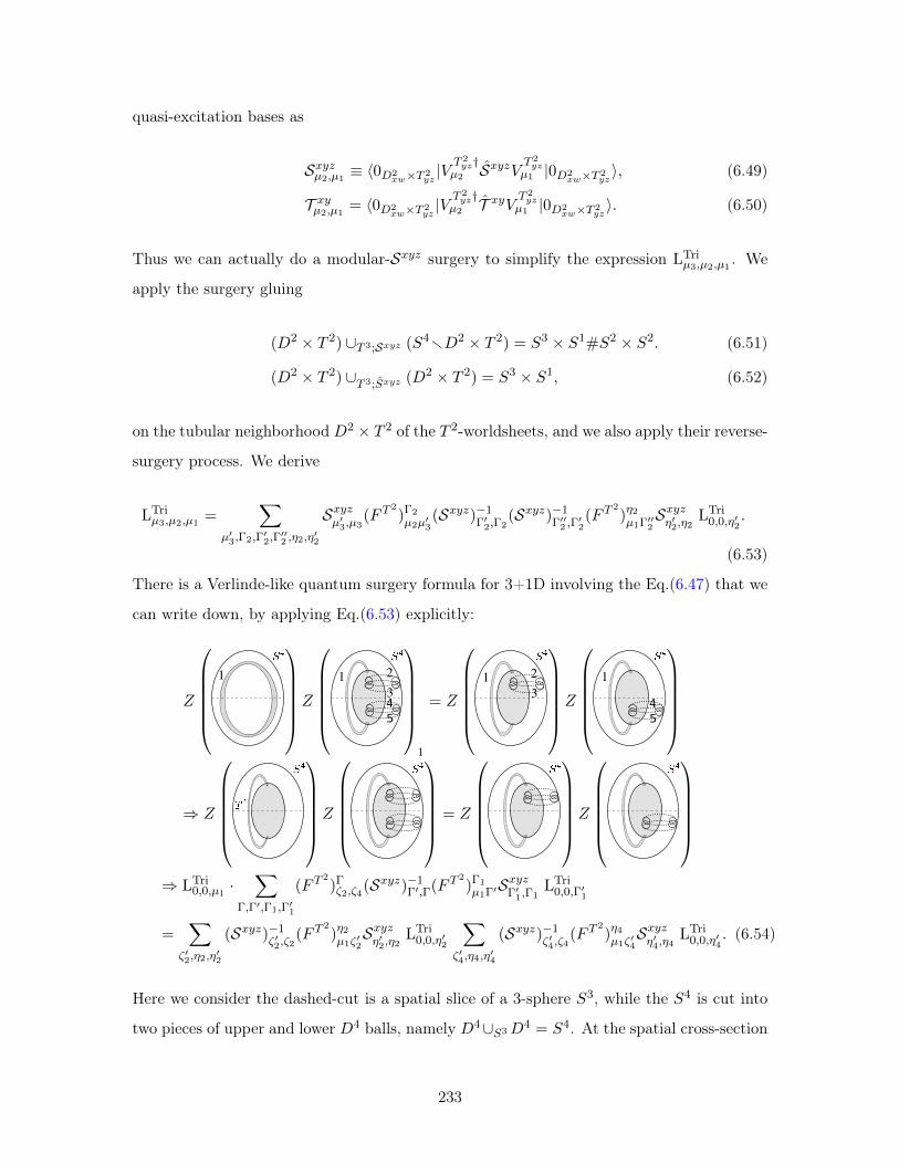
quasi-excitation bases as
𝒮𝑥𝑦𝑧𝜇2,𝜇1 ≡ ⟨0𝐷2𝑥𝑤×𝑇 2
𝑦𝑧|𝑉 𝑇 2
𝑦𝑧†𝜇2 𝒮𝑥𝑦𝑧𝑉 𝑇 2
𝑦𝑧𝜇1 |0𝐷2
𝑥𝑤×𝑇 2𝑦𝑧⟩, (6.49)
𝒯 𝑥𝑦𝜇2,𝜇1 = ⟨0𝐷2𝑥𝑤×𝑇 2
𝑦𝑧|𝑉 𝑇 2
𝑦𝑧†𝜇2 𝒯 𝑥𝑦𝑉 𝑇 2
𝑦𝑧𝜇1 |0𝐷2
𝑥𝑤×𝑇 2𝑦𝑧⟩. (6.50)
Thus we can actually do a modular-𝒮𝑥𝑦𝑧 surgery to simplify the expression LTri𝜇3,𝜇2,𝜇1 . We
apply the surgery gluing
(𝐷2 × 𝑇 2) ∪𝑇 3;𝒮𝑥𝑦𝑧 (𝑆4r𝐷2 × 𝑇 2) = 𝑆3 × 𝑆1#𝑆2 × 𝑆2. (6.51)
(𝐷2 × 𝑇 2) ∪𝑇 3;𝑆𝑥𝑦𝑧 (𝐷2 × 𝑇 2) = 𝑆3 × 𝑆1, (6.52)
on the tubular neighborhood 𝐷2 × 𝑇 2 of the 𝑇 2-worldsheets, and we also apply their reverse-
surgery process. We derive
LTri𝜇3,𝜇2,𝜇1 =
∑𝜇′3,Γ2,Γ′
2,Γ′′2 ,𝜂2,𝜂
′2
𝒮𝑥𝑦𝑧𝜇′3,𝜇3
(𝐹 𝑇2)Γ2
𝜇2𝜇′3(𝒮𝑥𝑦𝑧)−1
Γ′2,Γ2
(𝒮𝑥𝑦𝑧)−1Γ′′2 ,Γ
′2(𝐹 𝑇
2)𝜂2𝜇1Γ′′
2𝒮𝑥𝑦𝑧𝜂′2,𝜂2
LTri0,0,𝜂′2
.
(6.53)
There is a Verlinde-like quantum surgery formula for 3+1D involving the Eq.(6.47) that we
can write down, by applying Eq.(6.53) explicitly:
𝑍
⎛⎜⎜⎜⎜⎜⎝1
⎞⎟⎟⎟⎟⎟⎠𝑍
⎛⎜⎜⎜⎜⎜⎝1 2
345
⎞⎟⎟⎟⎟⎟⎠1
= 𝑍
⎛⎜⎜⎜⎜⎜⎝1 2
3
⎞⎟⎟⎟⎟⎟⎠𝑍
⎛⎜⎜⎜⎜⎜⎝1
45
⎞⎟⎟⎟⎟⎟⎠
⇒ 𝑍
⎛⎜⎜⎜⎜⎜⎝
⎞⎟⎟⎟⎟⎟⎠𝑍
⎛⎜⎜⎜⎜⎜⎝
⎞⎟⎟⎟⎟⎟⎠ = 𝑍
⎛⎜⎜⎜⎜⎜⎝
⎞⎟⎟⎟⎟⎟⎠𝑍
⎛⎜⎜⎜⎜⎜⎝
⎞⎟⎟⎟⎟⎟⎠⇒ LTri
0,0,𝜇1 ·∑
Γ,Γ′,Γ1,Γ′1
(𝐹 𝑇2)Γ𝜁2,𝜁4(𝒮
𝑥𝑦𝑧)−1Γ′,Γ(𝐹
𝑇 2)Γ1𝜇1Γ′𝒮𝑥𝑦𝑧Γ′
1,Γ1LTri0,0,Γ′
1
=∑
𝜁′2,𝜂2,𝜂′2
(𝒮𝑥𝑦𝑧)−1𝜁′2,𝜁2
(𝐹 𝑇2)𝜂2𝜇1𝜁′2𝒮𝑥𝑦𝑧𝜂′2,𝜂2
LTri0,0,𝜂′2
∑𝜁′4,𝜂4,𝜂
′4
(𝒮𝑥𝑦𝑧)−1𝜁′4,𝜁4
(𝐹 𝑇2)𝜂4𝜇1𝜁′4𝒮𝑥𝑦𝑧𝜂′4,𝜂4
LTri0,0,𝜂′4
. (6.54)
Here we consider the dashed-cut is a spatial slice of a 3-sphere 𝑆3, while the 𝑆4 is cut into
two pieces of upper and lower 𝐷4 balls, namely 𝐷4∪𝑆3𝐷4 = 𝑆4. At the spatial cross-section
233
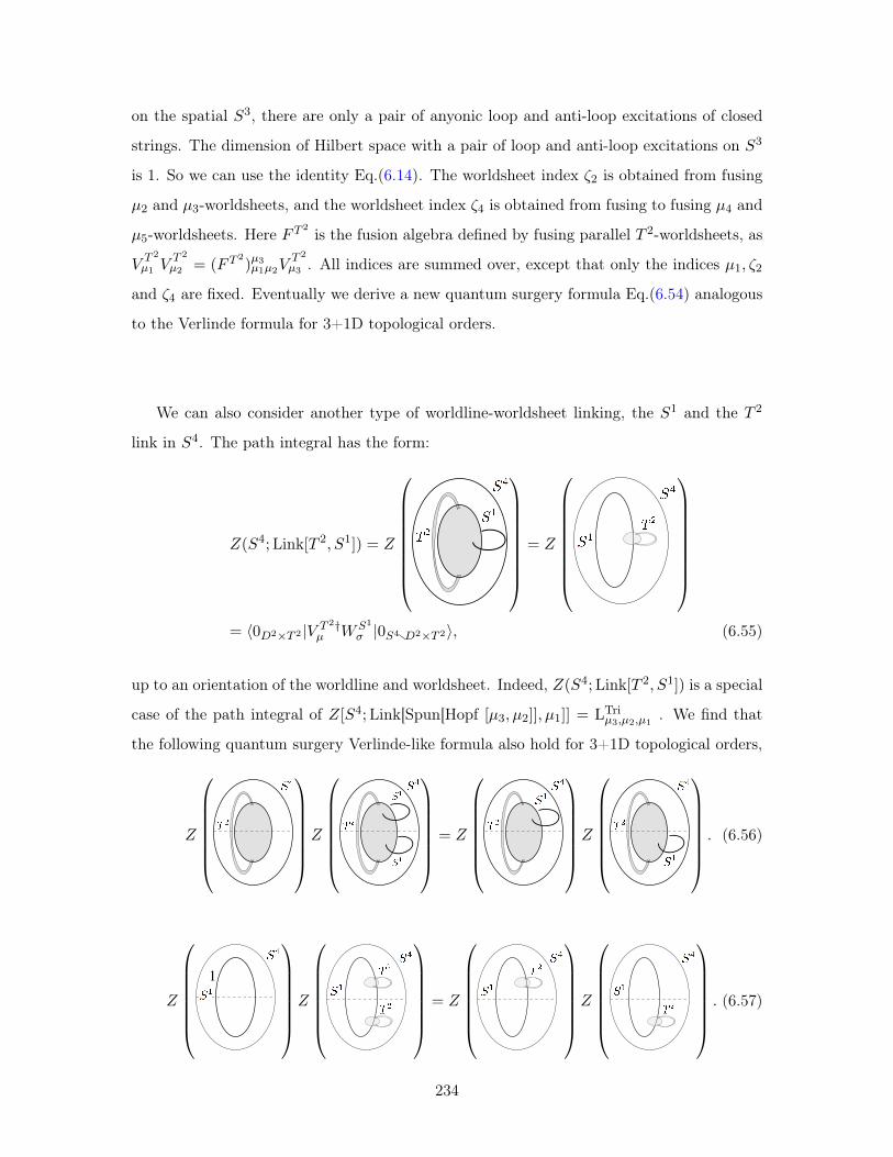
on the spatial 𝑆3, there are only a pair of anyonic loop and anti-loop excitations of closed
strings. The dimension of Hilbert space with a pair of loop and anti-loop excitations on 𝑆3
is 1. So we can use the identity Eq.(6.14). The worldsheet index 𝜁2 is obtained from fusing
𝜇2 and 𝜇3-worldsheets, and the worldsheet index 𝜁4 is obtained from fusing to fusing 𝜇4 and
𝜇5-worldsheets. Here 𝐹 𝑇 2 is the fusion algebra defined by fusing parallel 𝑇 2-worldsheets, as
𝑉𝑇 2
𝜇1 𝑉𝑇 2
𝜇2 = (𝐹 𝑇2)𝜇3𝜇1𝜇2𝑉
𝑇 2
𝜇3 . All indices are summed over, except that only the indices 𝜇1, 𝜁2
and 𝜁4 are fixed. Eventually we derive a new quantum surgery formula Eq.(6.54) analogous
to the Verlinde formula for 3+1D topological orders.
We can also consider another type of worldline-worldsheet linking, the 𝑆1 and the 𝑇 2
link in 𝑆4. The path integral has the form:
𝑍(𝑆4;Link[𝑇 2, 𝑆1]) = 𝑍
⎛⎜⎜⎜⎜⎜⎜⎜⎜⎝
⎞⎟⎟⎟⎟⎟⎟⎟⎟⎠= 𝑍
⎛⎜⎜⎜⎜⎜⎜⎜⎜⎝
⎞⎟⎟⎟⎟⎟⎟⎟⎟⎠= ⟨0𝐷2×𝑇 2 |𝑉 𝑇 2†
𝜇 𝑊𝑆1
𝜎 |0𝑆4r𝐷2×𝑇 2⟩, (6.55)
up to an orientation of the worldline and worldsheet. Indeed, 𝑍(𝑆4;Link[𝑇 2, 𝑆1]) is a special
case of the path integral of 𝑍[𝑆4;Link[Spun[Hopf [𝜇3, 𝜇2]], 𝜇1]] = LTri𝜇3,𝜇2,𝜇1 . We find that
the following quantum surgery Verlinde-like formula also hold for 3+1D topological orders,
𝑍
⎛⎜⎜⎜⎜⎜⎜⎝
⎞⎟⎟⎟⎟⎟⎟⎠𝑍
⎛⎜⎜⎜⎜⎜⎜⎝
⎞⎟⎟⎟⎟⎟⎟⎠ = 𝑍
⎛⎜⎜⎜⎜⎜⎜⎝
⎞⎟⎟⎟⎟⎟⎟⎠𝑍
⎛⎜⎜⎜⎜⎜⎜⎝
⎞⎟⎟⎟⎟⎟⎟⎠ . (6.56)
𝑍
⎛⎜⎜⎜⎜⎜⎜⎝1
⎞⎟⎟⎟⎟⎟⎟⎠𝑍
⎛⎜⎜⎜⎜⎜⎜⎝
⎞⎟⎟⎟⎟⎟⎟⎠ = 𝑍
⎛⎜⎜⎜⎜⎜⎜⎝
⎞⎟⎟⎟⎟⎟⎟⎠𝑍
⎛⎜⎜⎜⎜⎜⎜⎝
⎞⎟⎟⎟⎟⎟⎟⎠ . (6.57)
234
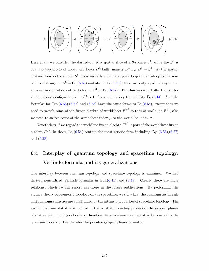
𝑍
⎛⎜⎜⎜⎜⎜⎜⎝
⎞⎟⎟⎟⎟⎟⎟⎠𝑍
⎛⎜⎜⎜⎜⎜⎜⎝
⎞⎟⎟⎟⎟⎟⎟⎠ = 𝑍
⎛⎜⎜⎜⎜⎜⎜⎝
⎞⎟⎟⎟⎟⎟⎟⎠𝑍
⎛⎜⎜⎜⎜⎜⎜⎜⎝
⎞⎟⎟⎟⎟⎟⎟⎟⎠.(6.58)
Here again we consider the dashed-cut is a spatial slice of a 3-sphere 𝑆3, while the 𝑆4 is
cut into two pieces of upper and lower 𝐷4 balls, namely 𝐷4 ∪𝑆3 𝐷4 = 𝑆4. At the spatial
cross-section on the spatial 𝑆3, there are only a pair of anyonic loop and anti-loop excitations
of closed strings on 𝑆3 in Eq.(6.56) and also in Eq.(6.58), there are only a pair of anyon and
anti-anyon excitations of particles on 𝑆3 in Eq.(6.57). The dimension of Hilbert space for
all the above configurations on 𝑆3 is 1. So we can apply the identity Eq.(6.14). And the
formulas for Eqs.(6.56),(6.57) and (6.58) have the same forms as Eq.(6.54), except that we
need to switch some of the fusion algebra of worldsheet 𝐹 𝑇 2 to that of worldline 𝐹𝑆1 , also
we need to switch some of the worldsheet index 𝜇 to the worldline index 𝜎.
Nonetheless, if we regard the worldline fusion algebra 𝐹𝑆1 is part of the worldsheet fusion
algebra 𝐹 𝑇 2 , in short, Eq.(6.54) contain the most generic form including Eqs.(6.56),(6.57)
and (6.58).
6.4 Interplay of quantum topology and spacetime topology:
Verlinde formula and its generalizations
The interplay between quantum topology and spacetime topology is examined. We had
derived generalized Verlinde formulas in Eqs.(6.41) and (6.45). Clearly there are more
relations, which we will report elsewhere in the future publications. By performing the
surgery theory of geometric-topology on the spacetime, we show that the quantum fusion rule
and quantum statistics are constrained by the intrinsic properties of spacetime topology. The
exotic quantum statistics is defined in the adiabatic braiding process in the gapped phases
of matter with topological orders, therefore the spacetime topology strictly constrains the
quantum topology thus dictates the possible gapped phases of matter.
235
236
Chapter 7
Conclusion: Finale and A New View
of Emergence-Reductionism
Thus far we have explored some physical properties and mathematical structures of topo-
logical states of matter of SPTs and topological orders (TOs). We have started from the
very basic notion of quantum mechanical Berry’s geometric phase, to reveal its profound
connection to many-body topological states of matter. For example, we use geometric phase
and geometric matrix to define modular 𝒮 and 𝒯 matrices which connects to the braiding
statistics of quasi-excitations of TOs, or the SPT invariants such as fractionalized charges
and degenerate zero modes from symmetry-twists of SPTs.
One important ingredient of our work is that the constraints of topologies and the mean-
ing of topologies. We can roughly distinguish them into three types: SPT topology (“classi-
cal” topology), TO topology (quantum topology) and spacetime topology. Our understand-
ing now is developed much beyond what was previewed in Chap.1. We summarize in Table
7.1.
One important message is that, when we combine the concepts of SPT topology (a sort of
“classical” topology compared to the TOs) and spacetime topology, we are able to constrain,
characterize and classify the possible types of SPT probes as symmetry-twists having branch
cuts on the spacetime manifold (Chap.3). This way of thinking leads us to regard the SPTs
as having a closer tie to the spacetime topology. SPTs are not merely some quantum matter
by itself, but quantum matter with symmetry-protection tied to the spacetime topology.
237
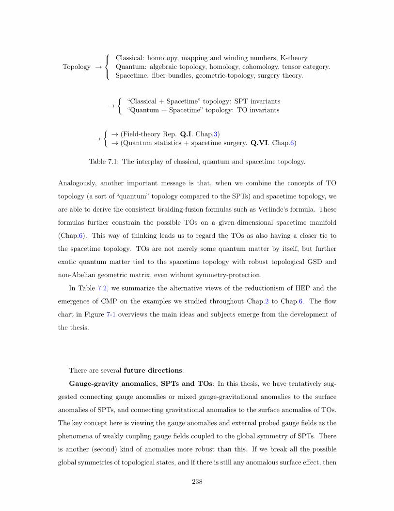
Topology →
⎧⎨⎩Classical: homotopy, mapping and winding numbers, K-theory.Quantum: algebraic topology, homology, cohomology, tensor category.Spacetime: fiber bundles, geometric-topology, surgery theory.
→{
“Classical + Spacetime” topology: SPT invariants“Quantum + Spacetime” topology: TO invariants
→{→ (Field-theory Rep. Q.I. Chap.3)→ (Quantum statistics + spacetime surgery. Q.VI. Chap.6)
Table 7.1: The interplay of classical, quantum and spacetime topology.
Analogously, another important message is that, when we combine the concepts of TO
topology (a sort of “quantum” topology compared to the SPTs) and spacetime topology, we
are able to derive the consistent braiding-fusion formulas such as Verlinde’s formula. These
formulas further constrain the possible TOs on a given-dimensional spacetime manifold
(Chap.6). This way of thinking leads us to regard the TOs as also having a closer tie to
the spacetime topology. TOs are not merely some quantum matter by itself, but further
exotic quantum matter tied to the spacetime topology with robust topological GSD and
non-Abelian geometric matrix, even without symmetry-protection.
In Table 7.2, we summarize the alternative views of the reductionism of HEP and the
emergence of CMP on the examples we studied throughout Chap.2 to Chap.6. The flow
chart in Figure 7-1 overviews the main ideas and subjects emerge from the development of
the thesis.
There are several future directions:
Gauge-gravity anomalies, SPTs and TOs: In this thesis, we have tentatively sug-
gested connecting gauge anomalies or mixed gauge-gravitational anomalies to the surface
anomalies of SPTs, and connecting gravitational anomalies to the surface anomalies of TOs.
The key concept here is viewing the gauge anomalies and external probed gauge fields as the
phenomena of weakly coupling gauge fields coupled to the global symmetry of SPTs. There
is another (second) kind of anomalies more robust than this. If we break all the possible
global symmetries of topological states, and if there is still any anomalous surface effect, then
238
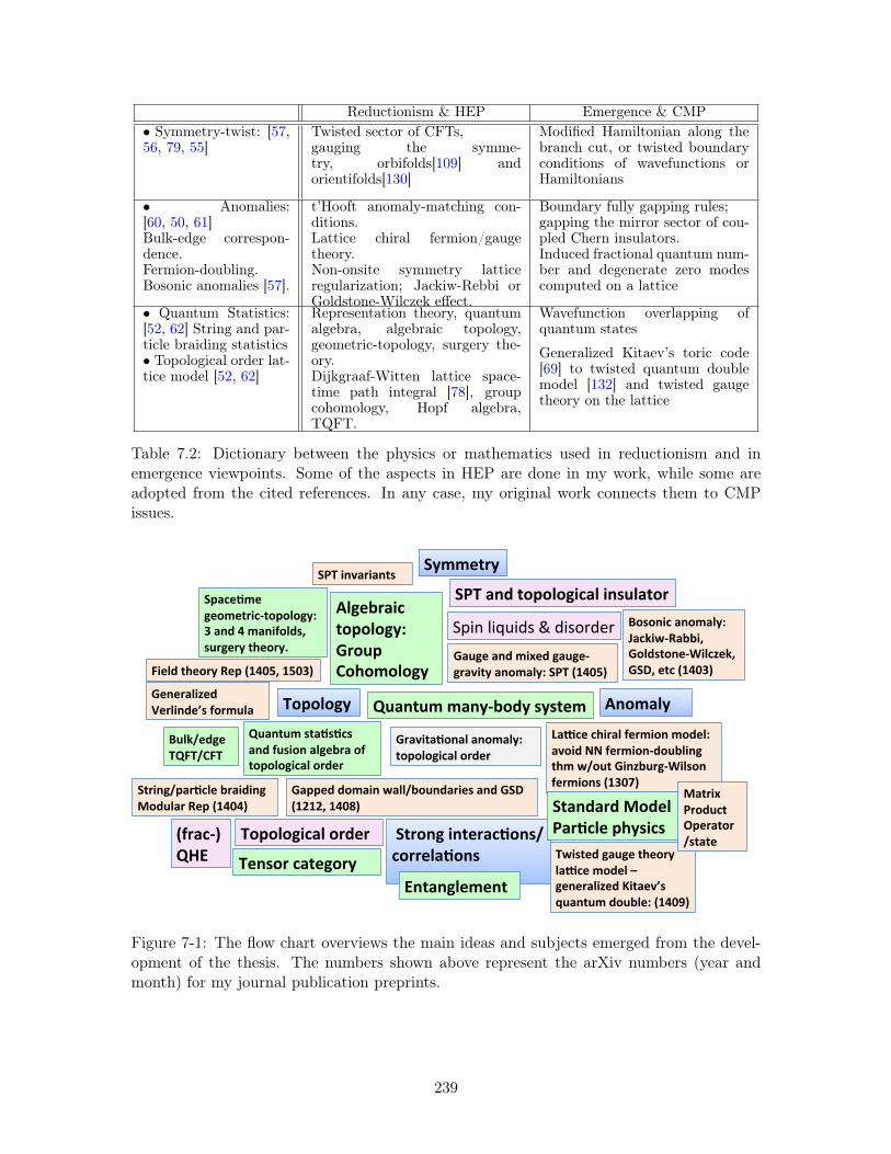
Reductionism & HEP Emergence & CMP∙ Symmetry-twist: [57,56, 79, 55]
Twisted sector of CFTs,gauging the symme-try, orbifolds[109] andorientifolds[130]
Modified Hamiltonian along thebranch cut, or twisted boundaryconditions of wavefunctions orHamiltonians
∙ Anomalies:[60, 50, 61]Bulk-edge correspon-dence.Fermion-doubling.Bosonic anomalies [57].
t’Hooft anomaly-matching con-ditions.Lattice chiral fermion/gaugetheory.Non-onsite symmetry latticeregularization; Jackiw-Rebbi orGoldstone-Wilczek effect.
Boundary fully gapping rules;gapping the mirror sector of cou-pled Chern insulators.Induced fractional quantum num-ber and degenerate zero modescomputed on a lattice
∙ Quantum Statistics:[52, 62] String and par-ticle braiding statistics∙ Topological order lat-tice model [52, 62]
Representation theory, quantumalgebra, algebraic topology,geometric-topology, surgery the-ory.Dijkgraaf-Witten lattice space-time path integral [78], groupcohomology, Hopf algebra,TQFT.
Wavefunction overlapping ofquantum states
Generalized Kitaev’s toric code[69] to twisted quantum doublemodel [132] and twisted gaugetheory on the lattice
Table 7.2: Dictionary between the physics or mathematics used in reductionism and inemergence viewpoints. Some of the aspects in HEP are done in my work, while some areadopted from the cited references. In any case, my original work connects them to CMPissues.
!"##$%&"'
()*)+),"' -.)#/+"'
'!%&).,'0.%$&/12).34'
1)&&$+/2).3'
!*/1$2#$'
,$)#$%&015%)*)+),"6'
7'/.8'9'#/.0:)+83;'
3<&,$&"'%=$)&">''
!?('0.@/&0/.%3'
A0$+8'%=$)&"'B$*'CD9EF;'DFE7G'
H</.%<#'3%/23213'
/.8':<30).'/+,$I&/'):'
%)*)+),01/+')&8$&'
J$.$&/+0K$8'
L$&+0.8$M3':)&#<+/'
J/<,$'/.8'#0N$8',/<,$5
,&/@0%"'/.)#/+"6'!?('CD9EFG'
J&/@0%/2)./+'/.)#/+"6'
%)*)+),01/+')&8$&''
H</.%<#'#/."5I)8"'3"3%$#'
O/P1$'1=0&/+':$�).'#)8$+6''
/@)08'QQ':$�).58)<I+0.,''
%=#'R4)<%'J0.KI<&,5S0+3).''
:$�).3'CD7ETG'J/**$8'8)#/0.'R/++4I)<.8/&0$3'/.8'J!U'
CDVDV;'D9EWG'
X)3).01'/.)#/+"6''
Y/1Z0R5B/II0;''
J)+83%).$5S0+1K$Z;''
J!U;'$%1'CD9E7G'
!%&0.,4*/&21+$'I&/080.,'
[)8<+/&'B$*'CD9E9G'
(R03%$8',/<,$'%=$)&"'
+/P1$'#)8$+'\'
,$.$&/+0K$8']0%/$@M3'
^</.%<#'8)<I+$6'CD9E_G'
()*)+),01/+')&8$&'
!%/.8/&8'[)8$+'
?/&21+$'*="3013'
-+,$I&/01'
%)*)+),"6'
J&)<*'
`)=)#)+),"'
X<+Z4$8,$''
(HA(4`A('
($.3)&'1/%$,)&"'
!"#$%&#'(#)*%+%)#*,-).-%
!?('/.8'%)*)+),01/+'0.3<+/%)&'
C:&/15G''
Hab'
Final
b.%/.,+$#$.%'
[/%&0N''
?&)8<1%'
c*$&/%)&'
43%/%$'
Figure 7-1: The flow chart overviews the main ideas and subjects emerged from the devel-opment of the thesis. The numbers shown above represent the arXiv numbers (year andmonth) for my journal publication preprints.
239
these anomalies do not need to be protected by global symmetries. Thus, they are more
robust than gauge anomalies. They are associated with spacetime diffeomorphism. They
can be viewed as gravitational anomalies — including perturbative gravitational anoma-
lies (computable from a 1-loop Feynman diagram) or non-perturbative global gravitational
anomalies. We understand that so far we have only studied some examples to support this
claim. It will be helpful to find more new examples to test and clarify this claim.
Experimental or numerical realization of phases of matter: It will be important
to find the materialization through correlated quantum magnets, electronic Mott insulators
and ultra-cold atoms. It seems that a complete theory on the classification of interact-
ing SPTs and topological insulators/superconductors is still missing [33]. Several steps of
progress have been made in specific examples. What we are searching for a consistent-
complete theory is like the Ginzburg-Landau’s group theory for symmetry-breaking phases,
and the tensor category theory for 2D TOs. Whether we have the group-cohomology or
cobordism theory or something else to classify SPTs, and what theory we should develop to
fully classify higher-dimensional TOs, are the open challenges to be tackled in the future.
Non-perturbative lattice chiral fermion: We have proposed a simple model for a
non-perturbative lattice chiral fermion model. Currently three main attempts to regularize
the following chiral theory on the lattice are: (i) U(1) chiral fermion [50], (ii) SO(10) chiral
gauge [127] and (iii) U(1)×𝑍2×𝑍𝑇2 interacting topological superconductor theory [133]. Our
anomaly-free proof for U(1) chiral fermions is the most rigorous among the three, thanks to
the bosonization technique in 1D. The possible next step will be concretely proving that an
anomaly-free SM-like chiral gauge theory can be constructed using the mirror-decoupling
set-up, by looking into larger extra symmetries as we did in [50] outside a tentative gauge
group SO(10) or SU(5). One can search for the potential hidden constraints on the param-
eters of SM or modified-SM when it can be defined non-perturbatively on the lattice, such
as the Higgs scale and top quark mass. This may help to address beyond-SM questions,
such as hierarchy or strong CP problems. There is also the possibility of synthesizing the
idea of mirror-fermion decoupling with other HEP theories with extra dimensions, such as
Kaluza-Klein, Einstein-Bergmann and Randall-Sundrum models. The second issue for this
goal is to implement the simplest 1+1D chiral theory on the lattice. The first attempt
can be programming the tensor network code, using 1D Matrix Product States (MPS) or
Density Matrix Renormalization Group (DMRG). If it is possible, the future directions are
240
(1) inventing a new algorithm which can solve a gapless system, going beyond the gapped
one of DMRG, or (2) seeking collaboration with simulation experts in many-body quantum
systems or in lattice QCD. A new algorithm is desirable and profound because the gapless
chiral fermions are highly-entangled states with an entropy 𝑆 ∝ 𝐿𝑑−1 log(𝐿) beyond-the-
area-law (𝐿 is the length dimension in 𝑑-D), which require a new ground state wavefunction
ansatz and a new simulation theory, such as the Multi-scale Entanglement Renormalization
Ansatz (MERA).
More general statements about anomaly-matching conditions and topological
gapping criteria for higher dimensional theory. In Chap.4 and Chap.5, we discuss
the 1+1D statement between anomaly-matching conditions and topological gapping criteria
with U(1)𝑛 symmetry. This concept may hold more generally than the given spacetime
and the given symmetry. It will be remarkable to extend this direction further. It may
be useful to understand the characterization by entanglement entropy (EE), in particular
topological entanglement entropy (TEE). One key feature of topological orders is known
to be their long-range entanglement. TEE shows how quantum wavefunctions can be cor-
related to each other remotely through the entanglement. Up till now, people have been
looking at TEE on the system either at a closed manifold or at the interior without physical
boundaries. Building upon our previous work on gapped boundaries/domain walls [60, 61],
we can investigate EE and TEE on the system on generic open or closed manifolds. It
is an important question, because the gappability of boundary is related to the ’t Hooft
anomaly-matching conditions of gauge anomalies or (perturbative or global) gravitational
anomalies. From the reductionism aspect in HEP, the anomaly-matching is the mechanism
of the anomaly-inflow. However, from the emergence aspect in CMP, the same concept is
analogous to Laughlin’s flux insertion Gedanken-experiment. One can also check how EE
fits into the mirror-fermion decoupling set-up, and whether the gapped mirror sector (set
at the Planck scale) constrains the light sector with nearly gapless fermions. HEP tends to
view gauge theory as governed by “gauge symmetry,” but indeed it has no real symmetries
only redundancies. Ultimately, we can view gauge theory through entanglement. We should
understand how the SM structure can be embedded and ask how new entanglement concepts
beyond EE or TEE can be introduced for strongly-interacting gapless phases.
Topological phase transitions and gapless phases: The topological gapping criteria
for gapped domain walls located between TOs Phases 𝐴 and 𝐵, may be connected to the
241

topological phase transitions between TOs Phases 𝐴 and 𝐵. Topological phase transitions
here may not just include the first order phase transition, but also the second order phase
transition. It will be important to see whether extra conditions should be included to derive
the criteria for the second order phase transitions. This information could provide one of
crucial hints for studying robust gapless phases of matter. Another crucial hints can be the
surface gapless states due to anomalies protected by the bulk state of matter.
Further interplay of the spacetime topology and the states of matter topology:
It is likely the approach on spacetime surgery and the quantum amplitudes can be generalized
to study not just TOs but also SPTs, or more generally symmetry-enriched topological states
(SETs, for topological orders with symmetry-protection). There should be a direct program
generalized by extending Chap. 3 to 6.
Many-body entanglement structure: Throughout the thesis, the hidden concept
of entanglement is used, but we have not yet explicitly studied it in depth. Whether the
result we obtained so far (such as anomaly-matching and gapping criteria, string braiding
statistics and generalized Verlinde formula) can be organized in terms of the fundamental
principles of quantum entanglement structure will be left for future questions.
If we digest the reductionism and emergence viewpoints further, the two views are rather
different, but there is not actually an obvious cut between the two philosophies. The prin-
ciples emerging from a many-body system can be reduced to a few guiding principles and
the basic ingredients of qubits or spins and their interactions can be regarded as the funda-
mental blocks of reductionism (thus, emergence gives rise to reductionism). On the other
hand, it also happens that the fundamental laws of reductionism can be re-arranged and
transformed into another set of formulation where the fundamental ingredients are trans-
formed, too (such as the particle-wave duality; this is sort of reductionism gives rise to
emergence). This reminds us of the importance of complementarity of reductionism and
emergence. We should recall that Niels Bohr’s coat of arms, “opposites are complementary,”
and John Wheeler’s comment on complementarity: “Bohr’s principle of complementarity
is the most revolutionary scientific concept of this century and the heart of his fifty-year
search for the full significance of the quantum idea.” Perhaps to keep the two complemen-
tary viewpoints will guide us to digest the full profundity of the quantum world and the
beyond-quantum world.
242
Bibliography
[1] P. W. Anderson. More is different. Science, 177(4047):393–396, 1972.
[2] Sidney Coleman. Aspects of Symmetry. Cambridge University Press., 1988.
[3] E. Farhi and R. Jackiw. Dynamical Gauge Symmetry Breaking. A Collection OfReprints . 1982.
[4] S.B. Treiman, Edward Witten, R. Jackiw, and B. Zumino. Current Algebra AndAnomalies .
[5] F. Wilczek. Fractional Statistics and Anyon Superconductivity. International journalof modern physics. World Scientific, 1990.
[6] R. Jackiw. Diverse topics in theoretical and mathematical physics. 1995.
[7] Kenneth G. Wilson. The renormalization group: Critical phenomena and the kondoproblem. Rev. Mod. Phys., 47:773–840, Oct 1975.
[8] L. D. Landau. Theory of phase transformations. Phys. Z. Sowjetunion, 11:26 and 545,1937.
[9] V. L. Ginzburg and L. D. Landau. On the theory of superconductivity. Zh. Eksp.Teor. Fiz., 20:1064–1082, 1950.
[10] L. D. Landau and E. M. Lifschitz. Statistical Physics - Course of Theoretical PhysicsVol 5. Pergamon, London, 1958.
[11] X.G. Wen. Quantum Field Theory of Many-body Systems: From the Origin of Soundto an Origin of Light and Electrons. Oxford graduate texts. Oxford University Press,2004.
[12] Xie Chen, Zheng-Cheng Gu, Zheng-Xin Liu, and Xiao-Gang Wen. Symmetry-protected topological orders and the cohomology class of their symmetry group. Phys.Rev. B, 87:155114, 2013.
[13] Xie Chen, Zheng-Cheng Gu, Zheng-Xin Liu, and Xiao-Gang Wen. Symmetry protectedtopological orders in interacting bosonic systems. Science 338, 1604, 2012.
[14] Xiao-Gang Wen. Topological orders in rigid states. Int. J. Mod. Phys. B, 4:239, 1990.
[15] X.-G. Wen. Topological order: from long-range entangled quantum matter to anunification of light and electrons. ArXiv e-prints, October 2012.
243
[16] K. v. Klitzing, G. Dorda, and M. Pepper. New method for high-accuracy determinationof the fine-structure constant based on quantized hall resistance. Phys. Rev. Lett.,45:494–497, Aug 1980.
[17] D. C. Tsui, H. L. Stormer, and A. C. Gossard. Two-dimensional magnetotransport inthe extreme quantum limit. Phys. Rev. Lett., 48:1559–1562, 1982.
[18] R. B. Laughlin. Anomalous quantum hall effect: An incompressible quantum fluidwith fractionally charged excitations. Phys. Rev. Lett., 50:1395–1398, 1983.
[19] Alexei Kitaev. Anyons in an exactly solved model and beyond. Ann. Phys., 321:2,2006.
[20] John Preskill. Lecture notes for physics 229: Quantum information and computation.1998.
[21] J.K. Pachos. Introduction to Topological Quantum Computation. Introduction toTopological Quantum Computation. Cambridge University Press, 2012.
[22] Alexei Kitaev and John Preskill. Topological entanglement entropy. Phys. Rev. Lett.,96:110404, Mar 2006.
[23] Michael Levin and Xiao-Gang Wen. Detecting topological order in a ground statewave function. Phys. Rev. Lett., 96:110405, 2006.
[24] C. N. Yang. Concept of off-diagonal long-range order and the quantum phases of liquidhe and of superconductors. Rev. Mod. Phys., 34:694–704, Oct 1962.
[25] Edward Witten. Topological Quantum Field Theory. Commun.Math.Phys., 117:353,1988.
[26] Edward Witten. Quantum Field Theory and the Jones Polynomial. Com-mun.Math.Phys., 121:351–399, 1989.
[27] X.-G. Wen. Symmetry-protected topological invariants of symmetry-protected topo-logical phases of interacting bosons and fermions. Phys. Rev. B, 89(3):035147, January2014.
[28] L.-Y. Hung and X.-G. Wen. Universal symmetry-protected topological invariants forsymmetry-protected topological states. 2013.
[29] Juven C. Wang, Z.-C. Gu, and X.-G. Wen. Field-Theory Representation of Gauge-Gravity Symmetry-Protected Topological Invariants, Group Cohomology, and Beyond.Phys. Rev. Lett., 114(3):031601, January 2015.
[30] M. Z. Hasan and C. L. Kane. Colloquium: Topological insulators. Reviews of ModernPhysics, 82:3045–3067, October 2010.
[31] X.-L. Qi and S.-C. Zhang. Topological insulators and superconductors. Reviews ofModern Physics, 83:1057–1110, October 2011.
[32] A. M. Turner and A. Vishwanath. Beyond Band Insulators: Topology of Semi-metalsand Interacting Phases. ArXiv e-prints, January 2013.
244
[33] T. Senthil. Symmetry Protected Topological phases of Quantum Matter. ArXiv e-prints, May 2014.
[34] F. D. M. Haldane. Continuum dynamics of the 1-D heisenberg antiferromagnet: Iden-tification with the O(3) nonlinear sigma model. Physics Letters A, 93:464, 1983.
[35] I. Affleck, T. Kennedy, E. H. Lieb, and H. Tasaki. Commun. Math. Phys., 115:477,1988.
[36] J. E. Moore and L. Balents. Topological invariants of time-reversal-invariant bandstructures. Phys. Rev. B, 75(12):121306, 2007.
[37] Liang Fu, C. L. Kane, and E. J. Mele. Topological insulators in three dimensions.Phys. Rev. Lett., 98(10):106803, 2007.
[38] Rahul Roy. Topological phases and the quantum spin hall effect in three dimensions.Phys. Rev. B, 79(19):195322, 2009.
[39] C. L. Kane and E. J. Mele. Z2 topological order and the quantum spin hall effect.Phys. Rev. Lett., 95:146802, 2005.
[40] B. Andrei Bernevig, Taylor L. Hughes, and Shou-Cheng Zhang. Quantum spin halleffect and topological phase transition in hgte quantum wells. Science, 314(5806):1757–1761, 2006.
[41] M. König, S. Wiedmann, C. Brüne, A. Roth, H. Buhmann, L. W. Molenkamp, X.-L.Qi, and S.-C. Zhang. Quantum Spin Hall Insulator State in HgTe Quantum Wells.Science, 318:766–, November 2007.
[42] L. Fu. Topological Crystalline Insulators. Physical Review Letters, 106(10):106802,March 2011.
[43] T. H. Hsieh, H. Lin, J. Liu, W. Duan, A. Bansil, and L. Fu. Topological crystallineinsulators in the SnTe material class. Nature Communications, 3:982, July 2012.
[44] Y. Tanaka, Z. Ren, T. Sato, K. Nakayama, S. Souma, T. Takahashi, K. Segawa,and Y. Ando. Experimental realization of a topological crystalline insulator in SnTe.Nature Physics, 8:800–803, November 2012.
[45] P. Dziawa, B. J. Kowalski, K. Dybko, R. Buczko, A. Szczerbakow, M. Szot,E. Łusakowska, T. Balasubramanian, B. M. Wojek, M. H. Berntsen, O. Tjernberg,and T. Story. Topological crystalline insulator states in Pb1−𝑥Sn𝑥Se. Nature Materi-als, 11:1023–1027, December 2012.
[46] S.-Y. Xu, C. Liu, N. Alidoust, M. Neupane, D. Qian, I. Belopolski, J. D. Denlinger,Y. J. Wang, H. Lin, L. A. Wray, G. Landolt, B. Slomski, J. H. Dil, A. Marcinkova,E. Morosan, Q. Gibson, R. Sankar, F. C. Chou, R. J. Cava, A. Bansil, and M. Z.Hasan. Observation of a topological crystalline insulator phase and topological phasetransition in Pb1−𝑥Sn𝑥Te. Nature Communications, 3:1192, November 2012.
[47] Jr. Callan, Curtis G. and Jeffrey A. Harvey. Anomalies and Fermion Zero Modes onStrings and Domain Walls. Nucl.Phys., B250:427, 1985.
245
[48] Gerard ’t Hooft. Naturalness, chiral symmetry, and spontaneous chiral symmetrybreaking. NATO Sci.Ser.B, 59:135, 1980.
[49] Xiao-Gang Wen. Classifying gauge anomalies through symmetry-protected trivial or-ders and classifying gravitational anomalies through topological orders. Phys.Rev.,D88(4):045013, 2013.
[50] Juven Wang and Xiao-Gang Wen. A Lattice Non-Perturbative Hamiltonian Construc-tion of 1+1D Anomaly-Free Chiral Fermions and Bosons - on the equivalence of theanomaly matching conditions and the boundary fully gapping rules. 2013.
[51] Liang Kong and Xiao-Gang Wen. Braided fusion categories, gravitational anomalies,and the mathematical framework for topological orders in any dimensions. 2014.
[52] Juven Wang and Xiao-Gang Wen. Non-Abelian string and particle braiding in topo-logical order: Modular SL(3,Z) representation and (3+1) -dimensional twisted gaugetheory. Phys.Rev., B91(3):035134, 2015.
[53] Frank Wilczek and A. Zee. Appearance of Gauge Structure in Simple DynamicalSystems. Phys.Rev.Lett., 52:2111–2114, 1984.
[54] Holger Bech Nielsen and M. Ninomiya. Absence of Neutrinos on a Lattice. 1. Proofby Homotopy Theory. Nucl.Phys., B185:20, 1981.
[55] Zheng-Cheng Gu, Juven C. Wang, and Xiao-Gang Wen. Multi-kink topological termsand charge-binding domain-wall condensation induced symmetry-protected topologicalstates: Beyond Chern-Simons/BF theory. 2015.
[56] Juven Wang, Luiz H. Santos, and Xiao-Gang Wen. Bosonic Anomalies, Induced Frac-tional Quantum Numbers and Degenerate Zero Modes: the anomalous edge physicsof Symmetry-Protected Topological States. 2014.
[57] Luiz H. Santos and Juven Wang. Symmetry-protected many-body Aharonov-Bohmeffect. Phys.Rev., B89(19):195122, 2014.
[58] Stephen L. Adler. Axial vector vertex in spinor electrodynamics. Phys.Rev., 177:2426–2438, 1969.
[59] J.S. Bell and R. Jackiw. A PCAC puzzle: pi0 –> gamma gamma in the sigma model.Nuovo Cim., A60:47–61, 1969.
[60] Juven Wang and Xiao-Gang Wen. Boundary Degeneracy of Topological Order.Phys.Rev., B91(12):125124, 2015.
[61] Tian Lan, Juven C. Wang, and Xiao-Gang Wen. Gapped Domain Walls, GappedBoundaries and Topological Degeneracy. Phys.Rev.Lett., 114(7):076402, 2015.
[62] Yidun Wan, Juven C. Wang, and Huan He. Twisted Gauge Theory Model of Topo-logical Phases in Three Dimensions. 2014.
[63] R. Jackiw and C. Rebbi. Solitons with Fermion Number 1/2. Phys.Rev., D13:3398–3409, 1976.
246
[64] Jeffrey Goldstone and Frank Wilczek. Fractional Quantum Numbers on Solitons.Phys.Rev.Lett., 47:986–989, 1981.
[65] Michael Levin and Ady Stern. Phys. Rev. B, 86:115131, 2012.
[66] Y.-M. Lu and A. Vishwanath. Theory and classification of interacting integer topologi-cal phases in two dimensions: A Chern-Simons approach. Phys. Rev. B, 86(12):125119,September 2012.
[67] Peng Ye and Juven Wang. Symmetry-protected topological phases with charge andspin symmetries: Response theory and dynamical gauge theory in two and three di-mensions. Phys.Rev., B88(23):235109, 2013.
[68] Michael Levin. Protected edge modes without symmetry. Phys.Rev., X3(2):021009,2013.
[69] Alexei Yu Kitaev. Fault-tolerant quantum computation by anyons. Annals of Physics,303:2–30, 2003.
[70] Paul H. Ginsparg and Kenneth G. Wilson. A Remnant of Chiral Symmetry on theLattice. Phys.Rev., D25:2649, 1982.
[71] Kenneth G. Wilson. Confinement of Quarks. Phys.Rev., D10:2445–2459, 1974.
[72] Herbert Neuberger. Exactly massless quarks on the lattice. Phys.Lett., B417:141–144,1998.
[73] Herbert Neuberger. More about exactly massless quarks on the lattice. Phys.Lett.,B427:353–355, 1998.
[74] Pilar Hernandez, Karl Jansen, and Martin Luscher. Locality properties of Neuberger’slattice Dirac operator. Nucl.Phys., B552:363–378, 1999.
[75] Estia Eichten and John Preskill. Chiral Gauge Theories on the Lattice. Nucl.Phys.,B268:179, 1986.
[76] Chenjie Wang and Michael Levin. Braiding statistics of loop excitations in threedimensions. Phys.Rev.Lett., 113(8):080403, 2014.
[77] Shenghan Jiang, Andrej Mesaros, and Ying Ran. Generalized Modular Transforma-tions in (3+1)D Topologically Ordered Phases and Triple Linking Invariant of LoopBraiding. Phys.Rev., X4(3):031048, 2014.
[78] Robbert Dijkgraaf and Edward Witten. Topological Gauge Theories and Group Co-homology. Commun.Math.Phys., 129:393, 1990.
[79] Juven C. Wang, Zheng-Cheng Gu, and Xiao-Gang Wen. Field theory representationof gauge-gravity symmetry-protected topological invariants, group cohomology andbeyond. Phys.Rev.Lett., 114(3):031601, 2015.
[80] X.-G. Wen. Modular transformation and bosonic/fermionic topological orders inAbelian fractional quantum Hall states. 2012.
247
[81] F. D. M. Haldane and E. H. Rezayi. Periodic laughlin-jastrow wave functions for thefractional quantized hall effect. Phys. Rev. B, 31:2529–2531, 1985.
[82] E. Keski-Vakkuri and Xiao-Gang Wen. Ground state structure of hierarchical QHstates on torus and modular transformation. Int. J. Mod. Phys. B, 7:4227, 1993.
[83] Heidar Moradi and Xiao-Gang Wen. Universal wave function overlap and universaltopological data from generic gapped ground states. 2014.
[84] H. S. M. Coxeter and W. O. J. Moser. Generators and relations for discrete groups.Berlin-Gottingen-Heidelberg, Springer, 1957.
[85] Y. Zhang, T. Grover, A. Turner, M. Oshikawa, and A. Vishwanath. Quasiparticlestatistics and braiding from ground-state entanglement. Phys. Rev. B, 85(23):235151,June 2012.
[86] L. D. Landau and E. M. Lifschitz. Statistical Physics - Course of Theoretical PhysicsVol 5. Pergamon, London, 1958.
[87] Xiao-Liang Qi, Taylor Hughes, and Shou-Cheng Zhang. Topological Field Theory ofTime-Reversal Invariant Insulators. Phys.Rev., B78:195424, 2008.
[88] Anton Kapustin and Ryan Thorngren. Anomalies of discrete symmetries in threedimensions and group cohomology. Phys.Rev.Lett., 112(23):231602, 2014.
[89] Anton Kapustin and Ryan Thorngren. Anomalies of discrete symmetries in variousdimensions and group cohomology. 2014.
[90] Daniel S. Freed. Short-range entanglement and invertible field theories. 2014.
[91] A. Kapustin. Symmetry Protected Topological Phases, Anomalies, and Cobordisms:Beyond Group Cohomology. 2014.
[92] A. Kapustin. Bosonic Topological Insulators and Paramagnets: A view from cobor-disms. 2014.
[93] F. Verstraete, J. I. Cirac, J. I. Latorre, E. Rico, and M. M. Wolf. Renormalization-group transformations on quantum states. Phys. Rev. Lett., 94:140601, 2005.
[94] Guifre Vidal. Entanglement renormalization. Phys. Rev. Lett., 99:220405, 2007.
[95] M. Levin and Z.-C. Gu. Braiding statistics approach to symmetry-protected topolog-ical phases. Phys. Rev. B, 86:115109, 2012.
[96] Mark de Wild Propitius. Spontaneously broken Abelian Chern-Simons theories.Nucl.Phys., B489:297–359, 1997.
[97] Xie Chen and Xiao-Gang Wen. Chiral symmetry on the edge of 2D symmetry protectedtopological phases. Phys.Rev., B86:235135, 2012.
[98] Tian Lan and Xiao-Gang Wen. Topological quasiparticles and the holographic bulk-edge relation in (2+1) -dimensional string-net models. Phys.Rev., B90(11):115119,2014.
248
[99] Edward Witten. GLOBAL GRAVITATIONAL ANOMALIES. Commun.Math.Phys.,100:197, 1985.
[100] John B. Kogut. An Introduction to Lattice Gauge Theory and Spin Systems.Rev.Mod.Phys., 51:659, 1979.
[101] Michael A. Levin and Xiao-Gang Wen. String net condensation: A Physical mechanismfor topological phases. Phys.Rev., B71:045110, 2005.
[102] Andrej Mesaros and Ying Ran. Classification of symmetry enriched topological phaseswith exactly solvable models. Phys.Rev., B87(15):155115, 2013.
[103] Yuting Hu, Yidun Wan, and Yong-Shi Wu. Twisted quantum double model of topo-logical phases in two dimensions. Phys.Rev., B87(12):125114, 2013.
[104] D. Finkelstein and J. Rubinstein. Connection between spin, statistics, and kinks.J.Math.Phys., 9:1762–1779, 1968.
[105] C. Wang and M. Levin. Braiding statistics of loop excitations in three dimensions.2014.
[106] S. Jiang, A. Mesaros, and Y. Ran. Generalized modular transformations in 3+1Dtopologically ordered phases and triple linking invariant of loop braiding. 2014.
[107] Mark Dirk Frederik de Wild Propitius. Topological interactions in broken gauge the-ories. 1995.
[108] Heidar Moradi and Xiao-Gang Wen. Universal Topological Data for Gapped QuantumLiquids in Three Dimensions and Fusion Algebra for Non-Abelian String Excitations.Phys.Rev., B91(7):075114, 2015.
[109] O. M. Sule, X. Chen, and S. Ryu. Symmetry-protected topological phases and orb-ifolds: Generalized Laughlin’s argument. Phys. Rev. B, 88(7):075125, August 2013.
[110] T.D. Lee and Chen-Ning Yang. Question of Parity Conservation in Weak Interactions.Phys.Rev., 104:254–258, 1956.
[111] Holger Bech Nielsen and M. Ninomiya. Absence of Neutrinos on a Lattice. 2. IntuitiveTopological Proof. Nucl.Phys., B193:173, 1981.
[112] Holger Bech Nielsen and M. Ninomiya. No Go Theorem for Regularizing ChiralFermions. Phys.Lett., B105:219, 1981.
[113] J. B. Kogut. An introduction to lattice gauge theory and spin systems. Rev. Mod.Phys., 51:659 – 713, 1979.
[114] D. B. Kaplan. A Method for Simulating Chiral Fermions on the Lattice. Phys. Lett.B, 288:342, 1992.
[115] Y. Shamir. Chiral fermions from lattice boundaries. Nucl. Phys. B, 406:90, 1993.
[116] M. Lüscher. Abelian chiral gauge theories on the lattice with exact gauge invariance.Nucl. Phys. B, 549(99):295 – 334, 1999.
249
[117] H. Suzuki. Gauge Invariant Effective Action in Abelian Chiral Gauge Theory on theLattice. Prog. Theor. Phys, 101:1147 – 1154, 1999.
[118] E. Eichten and J. Preskill. Chiral gauge theories on the lattice. Nucl. Phys. B, 268:179,1986.
[119] I. Montvay. Mirror fermions in chiral gauge theories. Nucl. Phys. Proc. Suppl.,29BC:159, 1992.
[120] T. Bhattacharya, M. R. Martin, and E. Poppitz. Chiral Lattice Gauge Theories fromWarped Domain Walls and Ginsparg-Wilson Fermions. Phys. Rev. D, 74:085028, 2006.
[121] J. Giedt and E. Poppitz. Chiral Lattice Gauge Theories and The Strong CouplingDynamics of a Yukawa-Higgs Model with Ginsparg-Wilson Fermions. Journal of HighEnergy Physics, 10:76, 2007.
[122] J. Smit. Acta Phys. Pol., B17:531, 1986.
[123] M. Golterman, D. Petcher, and E. Rivas. Absence of Chiral Fermions in the Eichten–Preskill Model. Nucl. Phys. B, 395:596 – 622, 1993.
[124] L. Lin. Nondecoupling of Heavy Mirror-Fermion. Phys. Lett. B, 324:418 – 424, 1994.
[125] C. Chen, J. Giedt, and E. Poppitz. On the decoupling of mirror fermions. Journal ofHigh Energy Physics, 131:1304, 2013.
[126] T. Banks and A. Dabholkar. Decoupling a Fermion Whose Mass Comes from a YukawaCoupling: Nonperturbative Considerations. Phys. Rev. D, 46:4016 – 4028, 1992.
[127] Xiao-Gang Wen. A lattice non-perturbative definition of an SO(10) chiral gauge theoryand its induced standard model. Chin.Phys.Lett., 30:111101, 2013.
[128] D.J. Thouless, M. Kohmoto, M.P. Nightingale, and M. den Nijs. Quantized HallConductance in a Two-Dimensional Periodic Potential. Phys.Rev.Lett., 49:405–408,1982.
[129] Anton Kapustin and Natalia Saulina. Topological boundary conditions in abelianChern-Simons theory. Nucl.Phys., B845:393–435, 2011.
[130] C.-T. Hsieh, O. M. Sule, G. Y. Cho, S. Ryu, and R. G. Leigh. Symmetry-protectedtopological phases, generalized Laughlin argument, and orientifolds. Phys. Rev. B,90(16):165134, October 2014.
[131] Xiao-Gang Wen. Construction of bosonic symmetry-protected-trivial states and theirtopological invariants via 𝐺× 𝑆𝑂(∞) non-linear 𝜎-models. 2014.
[132] Y. Hu, Y. Wan, and Y.-S. Wu. Twisted quantum double model of topological phasesin two dimensions. Phys. Rev. B, 87(12):125114, March 2013.
[133] Yizhuang You, Yoni BenTov, and Cenke Xu. Interacting Topological Superconductorsand possible Origin of 16𝑛 Chiral Fermions in the Standard Model. 2014.
250