UNIVERSITE LIBRE DE BRUXELLESFaculte des Sciences

Departement de PhysiqueService de Physique Mathematique des Interactions Fondamentales

Aspects of higher spin Hamiltoniandynamics: Conformal geometry, duality

and chargesAmaury Leonard

Promoteur: These de doctorat presentee en vue deMarc Henneaux l’obtention du titre deJury: Docteur en SciencesGlenn BarnichXavier BekaertFrank FerrariAxel KleinschmidtMichel Tytgat

Annee academique 2016 - 2017

arX

iv:1

709.

0071

9v2

[m

ath-

ph]

3 O

ct 2

017

A Francois, Christian, Antigone et Gwladys

Contents

Acknowledgements ix

Credits x

Abstract xi

Resume xii

General conventions xiii

Introduction 1

I Review of fundamentals 8

1 Free higher spin gauge fields 91.1 Bosonic fields . . . . . . . . . . . . . . . . . . . . . . . . . . . . . . . . . . . . . . . 9

1.1.1 Flat background space-time . . . . . . . . . . . . . . . . . . . . . . . . . . . 91.1.2 Constantly curved background space-time . . . . . . . . . . . . . . . . . . . 13

1.2 Fermionic fields . . . . . . . . . . . . . . . . . . . . . . . . . . . . . . . . . . . . . . 131.2.1 Flat background space-time . . . . . . . . . . . . . . . . . . . . . . . . . . . 131.2.2 Constantly curved background space-time . . . . . . . . . . . . . . . . . . . 16

2 Hamiltonian formalism for constrained systems 182.1 Dirac formalism . . . . . . . . . . . . . . . . . . . . . . . . . . . . . . . . . . . . . . 18

2.1.1 From Lagrangian to Hamiltonian . . . . . . . . . . . . . . . . . . . . . . . . 182.1.2 Gauge systems . . . . . . . . . . . . . . . . . . . . . . . . . . . . . . . . . . 202.1.3 Second class constraints . . . . . . . . . . . . . . . . . . . . . . . . . . . . . 21

2.2 Illustrations of Dirac formalism . . . . . . . . . . . . . . . . . . . . . . . . . . . . . 222.2.1 Classical electromagnetism . . . . . . . . . . . . . . . . . . . . . . . . . . . 222.2.2 Linearized gravity . . . . . . . . . . . . . . . . . . . . . . . . . . . . . . . . 24

2.3 First order action . . . . . . . . . . . . . . . . . . . . . . . . . . . . . . . . . . . . . 262.3.1 General formalism . . . . . . . . . . . . . . . . . . . . . . . . . . . . . . . . 262.3.2 Illustration of constrained first order formalism: spin 3/2 gauge field on flat

space . . . . . . . . . . . . . . . . . . . . . . . . . . . . . . . . . . . . . . . 292.4 Surface charges . . . . . . . . . . . . . . . . . . . . . . . . . . . . . . . . . . . . . . 31

Appendices 332.A Invertibility of the second class constraints Poisson brackets matrix . . . . . . . . . 332.B Resolution of the momentum constraint . . . . . . . . . . . . . . . . . . . . . . . . 342.C Gauge invariance of the prepotential φkl . . . . . . . . . . . . . . . . . . . . . . . 35

3 Dualities 363.1 Electric-magnetic duality . . . . . . . . . . . . . . . . . . . . . . . . . . . . . . . . 36

3.1.1 Spin 1 . . . . . . . . . . . . . . . . . . . . . . . . . . . . . . . . . . . . . . . 363.1.2 Spin 2 . . . . . . . . . . . . . . . . . . . . . . . . . . . . . . . . . . . . . . . 37

3.2 Twisted self-duality conditions . . . . . . . . . . . . . . . . . . . . . . . . . . . . . 38

iv

3.2.1 Spin 1 . . . . . . . . . . . . . . . . . . . . . . . . . . . . . . . . . . . . . . . 383.2.2 Spin 2 . . . . . . . . . . . . . . . . . . . . . . . . . . . . . . . . . . . . . . . 40

II Bosonic higher spin on flat space 42

4 Conformal curvature in D = 3 434.1 Spin-s diffeomorphism invariance . . . . . . . . . . . . . . . . . . . . . . . . . . . . 43

4.1.1 Riemann tensor . . . . . . . . . . . . . . . . . . . . . . . . . . . . . . . . . . 444.1.2 Einstein tensor . . . . . . . . . . . . . . . . . . . . . . . . . . . . . . . . . . 45

4.2 Spin-s Weyl invariance . . . . . . . . . . . . . . . . . . . . . . . . . . . . . . . . . . 464.2.1 Schouten tensor . . . . . . . . . . . . . . . . . . . . . . . . . . . . . . . . . . 474.2.2 Cotton tensor . . . . . . . . . . . . . . . . . . . . . . . . . . . . . . . . . . . 484.2.3 Spin-2 . . . . . . . . . . . . . . . . . . . . . . . . . . . . . . . . . . . . . . . 494.2.4 Spin-3 . . . . . . . . . . . . . . . . . . . . . . . . . . . . . . . . . . . . . . . 494.2.5 Spin-4 . . . . . . . . . . . . . . . . . . . . . . . . . . . . . . . . . . . . . . . 50

4.3 Cotton tensor as a complete set of Weyl invariants . . . . . . . . . . . . . . . . . . 514.3.1 Spin 3 . . . . . . . . . . . . . . . . . . . . . . . . . . . . . . . . . . . . . . . 514.3.2 Spin 4 . . . . . . . . . . . . . . . . . . . . . . . . . . . . . . . . . . . . . . . 52

4.4 Cotton tensors as a complete set of transverse-traceless symmetric tensors . . . . . 524.4.1 The problem . . . . . . . . . . . . . . . . . . . . . . . . . . . . . . . . . . . 524.4.2 Spin 2 . . . . . . . . . . . . . . . . . . . . . . . . . . . . . . . . . . . . . . . 534.4.3 Higher spin . . . . . . . . . . . . . . . . . . . . . . . . . . . . . . . . . . . . 53

Appendices 554.A Generalized differential . . . . . . . . . . . . . . . . . . . . . . . . . . . . . . . . . . 55

4.A.1 p-forms . . . . . . . . . . . . . . . . . . . . . . . . . . . . . . . . . . . . . . 554.A.2 Beyond fully antisymmetric tensors . . . . . . . . . . . . . . . . . . . . . . . 55

4.B Complete set of gauge invariant functions . . . . . . . . . . . . . . . . . . . . . . . 574.B.1 Generalities . . . . . . . . . . . . . . . . . . . . . . . . . . . . . . . . . . . . 574.B.2 Spin-s Weyl invariance . . . . . . . . . . . . . . . . . . . . . . . . . . . . . . 58

5 Hamiltonian analysis 615.1 Spin-3 . . . . . . . . . . . . . . . . . . . . . . . . . . . . . . . . . . . . . . . . . . . 61

5.1.1 Hamiltonian and constraints . . . . . . . . . . . . . . . . . . . . . . . . . . 625.1.2 Gauge transformations . . . . . . . . . . . . . . . . . . . . . . . . . . . . . . 625.1.3 Momentum constraint . . . . . . . . . . . . . . . . . . . . . . . . . . . . . . 635.1.4 Hamiltonian constraint . . . . . . . . . . . . . . . . . . . . . . . . . . . . . 635.1.5 Hamiltonian action in terms of prepotentials . . . . . . . . . . . . . . . . . 64

5.2 Arbitrary spin . . . . . . . . . . . . . . . . . . . . . . . . . . . . . . . . . . . . . . . 655.2.1 Change of variables and momenta . . . . . . . . . . . . . . . . . . . . . . . 655.2.2 Gauge transformations . . . . . . . . . . . . . . . . . . . . . . . . . . . . . . 665.2.3 Hamiltonian and constraints . . . . . . . . . . . . . . . . . . . . . . . . . . 675.2.4 Solving the momentum constraint . . . . . . . . . . . . . . . . . . . . . . . 685.2.5 Solving the Hamiltonian constraint . . . . . . . . . . . . . . . . . . . . . . . 695.2.6 Hamiltonian Action in terms of prepotentials . . . . . . . . . . . . . . . . . 72

Appendices 745.A Prepotentials for even spins . . . . . . . . . . . . . . . . . . . . . . . . . . . . . . . 74

5.A.1 First Step . . . . . . . . . . . . . . . . . . . . . . . . . . . . . . . . . . . . . 745.A.2 Second Step . . . . . . . . . . . . . . . . . . . . . . . . . . . . . . . . . . . . 755.A.3 Third Step . . . . . . . . . . . . . . . . . . . . . . . . . . . . . . . . . . . . 755.A.4 Summary . . . . . . . . . . . . . . . . . . . . . . . . . . . . . . . . . . . . . 75

5.B Prepotentials for odd spins . . . . . . . . . . . . . . . . . . . . . . . . . . . . . . . 765.B.1 First Step . . . . . . . . . . . . . . . . . . . . . . . . . . . . . . . . . . . . . 765.B.2 Second Step . . . . . . . . . . . . . . . . . . . . . . . . . . . . . . . . . . . . 765.B.3 Third Step . . . . . . . . . . . . . . . . . . . . . . . . . . . . . . . . . . . . 76

5.C Conformally invariant Hamiltonian . . . . . . . . . . . . . . . . . . . . . . . . . . . 78

v

5.C.1 Even spin: s = 2n . . . . . . . . . . . . . . . . . . . . . . . . . . . . . . . . 785.C.2 Odd spin: s = 2n+ 1 . . . . . . . . . . . . . . . . . . . . . . . . . . . . . . 79

6 Twisted self-duality 806.1 Equations of motion in terms of Riemann tensor . . . . . . . . . . . . . . . . . . . 806.2 Covariant twisted self-duality . . . . . . . . . . . . . . . . . . . . . . . . . . . . . . 816.3 Electric and magnetic fields . . . . . . . . . . . . . . . . . . . . . . . . . . . . . . . 82

6.3.1 Definitions . . . . . . . . . . . . . . . . . . . . . . . . . . . . . . . . . . . . 826.3.2 Twisted self-duality in terms of electric and magnetic fields . . . . . . . . . 846.3.3 Getting rid of the Lagrange multipliers . . . . . . . . . . . . . . . . . . . . . 84

6.4 Variational principle . . . . . . . . . . . . . . . . . . . . . . . . . . . . . . . . . . . 856.4.1 Prepotentials . . . . . . . . . . . . . . . . . . . . . . . . . . . . . . . . . . . 856.4.2 Twisted self-duality and prepotentials . . . . . . . . . . . . . . . . . . . . . 856.4.3 Action . . . . . . . . . . . . . . . . . . . . . . . . . . . . . . . . . . . . . . . 85

Appendices 876.A Higher dimensions and twisted self-duality . . . . . . . . . . . . . . . . . . . . . . . 876.B Electric-magnetic duality . . . . . . . . . . . . . . . . . . . . . . . . . . . . . . . . 88

6.B.1 How the symmetries fix the action . . . . . . . . . . . . . . . . . . . . . . . 88

III Toward supersymmetry 90

7 Hypergravity and electric-magnetic duality 917.1 Covariant form of hypergravity . . . . . . . . . . . . . . . . . . . . . . . . . . . . . 92

7.1.1 Action . . . . . . . . . . . . . . . . . . . . . . . . . . . . . . . . . . . . . . . 927.1.2 Gauge symmetries . . . . . . . . . . . . . . . . . . . . . . . . . . . . . . . . 927.1.3 Supersymmetry . . . . . . . . . . . . . . . . . . . . . . . . . . . . . . . . . . 937.1.4 Equations of motion . . . . . . . . . . . . . . . . . . . . . . . . . . . . . . . 93

7.2 Hamiltonian form . . . . . . . . . . . . . . . . . . . . . . . . . . . . . . . . . . . . . 937.2.1 Spin-2 part . . . . . . . . . . . . . . . . . . . . . . . . . . . . . . . . . . . . 937.2.2 Spin-5/2 part . . . . . . . . . . . . . . . . . . . . . . . . . . . . . . . . . . . 94

7.3 Solving the constraints - Prepotentials . . . . . . . . . . . . . . . . . . . . . . . . . 957.4 Supersymmetry transformations in terms of the prepotentials . . . . . . . . . . . . 977.5 Action . . . . . . . . . . . . . . . . . . . . . . . . . . . . . . . . . . . . . . . . . . . 98

Appendices 997.A Technical derivations . . . . . . . . . . . . . . . . . . . . . . . . . . . . . . . . . . . 99

7.A.1 Bosonic prepotential Zmn2 = φmn . . . . . . . . . . . . . . . . . . . . . . . . 997.A.2 Bosonic prepotential Zmn1 = Pmn . . . . . . . . . . . . . . . . . . . . . . . . 1007.A.3 Supersymmetric variation of the fermionic prepotential Σij . . . . . . . . . 101

7.B The spin-(1, 32 ) multiplet . . . . . . . . . . . . . . . . . . . . . . . . . . . . . . . . . 103

7.B.1 Spin 1 . . . . . . . . . . . . . . . . . . . . . . . . . . . . . . . . . . . . . . . 1037.B.2 Spin 3/2 . . . . . . . . . . . . . . . . . . . . . . . . . . . . . . . . . . . . . . 1037.B.3 Supersymmetry . . . . . . . . . . . . . . . . . . . . . . . . . . . . . . . . . . 104

8 Beyond fully symmetric tensors: type (2, 2) 1058.1 Covariant description . . . . . . . . . . . . . . . . . . . . . . . . . . . . . . . . . . . 1058.2 Electric and magnetic fields . . . . . . . . . . . . . . . . . . . . . . . . . . . . . . . 1078.3 Prepotentials - Action . . . . . . . . . . . . . . . . . . . . . . . . . . . . . . . . . . 1088.4 Chiral and non-chiral actions . . . . . . . . . . . . . . . . . . . . . . . . . . . . . . 1108.5 Dimensional reduction . . . . . . . . . . . . . . . . . . . . . . . . . . . . . . . . . . 1108.6 Generalizations . . . . . . . . . . . . . . . . . . . . . . . . . . . . . . . . . . . . . . 110

Appendices 1128.A Equations of motion . . . . . . . . . . . . . . . . . . . . . . . . . . . . . . . . . . . 1128.B Hamiltonian formulation . . . . . . . . . . . . . . . . . . . . . . . . . . . . . . . . . 1138.C Dimensional reduction . . . . . . . . . . . . . . . . . . . . . . . . . . . . . . . . . . 114

vi

IV Surface charges on AdS 115

9 Bose fields 1169.1 Introduction . . . . . . . . . . . . . . . . . . . . . . . . . . . . . . . . . . . . . . . . 1169.2 Spin-3 example . . . . . . . . . . . . . . . . . . . . . . . . . . . . . . . . . . . . . . 116

9.2.1 Hamiltonian and constraints . . . . . . . . . . . . . . . . . . . . . . . . . . 1179.2.2 Gauge transformations . . . . . . . . . . . . . . . . . . . . . . . . . . . . . . 1189.2.3 Boundary conditions . . . . . . . . . . . . . . . . . . . . . . . . . . . . . . . 1199.2.4 Asymptotic symmetries . . . . . . . . . . . . . . . . . . . . . . . . . . . . . 1219.2.5 Charges . . . . . . . . . . . . . . . . . . . . . . . . . . . . . . . . . . . . . . 123

9.3 Arbitrary spin . . . . . . . . . . . . . . . . . . . . . . . . . . . . . . . . . . . . . . . 1259.3.1 Constraints and gauge transformations . . . . . . . . . . . . . . . . . . . . . 1259.3.2 Boundary conditions and asymptotic symmetries . . . . . . . . . . . . . . . 1289.3.3 Charges . . . . . . . . . . . . . . . . . . . . . . . . . . . . . . . . . . . . . . 129

9.4 Summary and further developments . . . . . . . . . . . . . . . . . . . . . . . . . . 130

Appendices 1329.A Notation and conventions . . . . . . . . . . . . . . . . . . . . . . . . . . . . . . . . 1329.B Hamiltonian form of Fronsdal’s action . . . . . . . . . . . . . . . . . . . . . . . . . 133

9.B.1 Spin 3 . . . . . . . . . . . . . . . . . . . . . . . . . . . . . . . . . . . . . . . 1339.B.2 Arbitrary spin . . . . . . . . . . . . . . . . . . . . . . . . . . . . . . . . . . 133

9.C Covariant boundary conditions . . . . . . . . . . . . . . . . . . . . . . . . . . . . . 1359.C.1 Falloff of the solutions of the free equations of motion . . . . . . . . . . . . 1359.C.2 Residual gauge symmetry . . . . . . . . . . . . . . . . . . . . . . . . . . . . 1369.C.3 Initial data at the boundary . . . . . . . . . . . . . . . . . . . . . . . . . . . 137

9.D Conformal Killing tensors . . . . . . . . . . . . . . . . . . . . . . . . . . . . . . . . 1399.E Spin-s charges . . . . . . . . . . . . . . . . . . . . . . . . . . . . . . . . . . . . . . . 141

10 Fermi fields 14310.1 Spin-5/2 example . . . . . . . . . . . . . . . . . . . . . . . . . . . . . . . . . . . . . 143

10.1.1 Hamiltonian and constraints . . . . . . . . . . . . . . . . . . . . . . . . . . 14410.1.2 Gauge transformations . . . . . . . . . . . . . . . . . . . . . . . . . . . . . . 14610.1.3 Boundary conditions . . . . . . . . . . . . . . . . . . . . . . . . . . . . . . . 14710.1.4 Asymptotic symmetries . . . . . . . . . . . . . . . . . . . . . . . . . . . . . 14810.1.5 Charges . . . . . . . . . . . . . . . . . . . . . . . . . . . . . . . . . . . . . . 15110.1.6 Three space-time dimensions . . . . . . . . . . . . . . . . . . . . . . . . . . 151

10.2 Arbitrary spin . . . . . . . . . . . . . . . . . . . . . . . . . . . . . . . . . . . . . . . 15210.2.1 Constraints and gauge transformations . . . . . . . . . . . . . . . . . . . . . 15210.2.2 Boundary conditions and asymptotic symmetries . . . . . . . . . . . . . . . 15410.2.3 Charges . . . . . . . . . . . . . . . . . . . . . . . . . . . . . . . . . . . . . . 156

10.3 Summary and further developments . . . . . . . . . . . . . . . . . . . . . . . . . . 157

Appendices 15910.A Notation and conventions . . . . . . . . . . . . . . . . . . . . . . . . . . . . . . . . 15910.B Covariant boundary conditions . . . . . . . . . . . . . . . . . . . . . . . . . . . . . 161

10.B.1 Falloff of the solutions of the free equations of motion . . . . . . . . . . . . 16110.B.2 Residual gauge symmetry . . . . . . . . . . . . . . . . . . . . . . . . . . . . 16210.B.3 Initial data at the boundary . . . . . . . . . . . . . . . . . . . . . . . . . . . 163

10.C Conformal Killing spinor-tensors . . . . . . . . . . . . . . . . . . . . . . . . . . . . 16510.C.1 Conformal Killing spinor-vectors . . . . . . . . . . . . . . . . . . . . . . . . 16510.C.2 Comments on arbitrary rank . . . . . . . . . . . . . . . . . . . . . . . . . . 16510.C.3 Independent conditions on asymptotic symmetries . . . . . . . . . . . . . . 166

Conclusion 169

vii

This thesis was defended behind closed doors on June 8th and publicly on July 3rd 2017, infront of the following jury at U.L.B., in Brussels:

• President: Prof. Frank Ferrari (Universite Libre de Bruxelles),

• Secretary: Prof. Glenn Barnich (Universite Libre de Bruxelles),

• Advisor: Prof. Marc Henneaux (Universite Libre de Bruxelles),

• Prof. Michel Tytgat (Universite Libre de Bruxelles),

• Dr. Xavier Bekaert (Universite Francois Rabelais),

• Dr. Axel Kleinschmidt (Max-Planck-Institut fur Gravitationsphysik).

Acknowledgements

If the writing of this thesis sometimes proved to be a long and winding path, it could not havebeen completed without the help and support of many people. Among them, the decisive role wascertainly played by my supervisor Marc Henneaux. For the swift efficiency, outstanding clarityand intellectual depth of his direction, advices, suggestions and explanations, for the kind, patientand generous presence he continuously offered during these years, I am eternally grateful.

My deepest thanks also go to Glenn Barnich, Xavier Bekaert, Frank Ferrari, Axel Kleinschmidtand Michel Tytgat, for accepting to constitute my jury and to bring forward the thoughts, com-mentaries and judgement this modest work inspired them. In addition, my gratitude goes to themregarding their long helping presence as elders and colleagues and, for many of them, as professors.

Many more of my colleagues deserve my heartfelt thanks under many regards, not only for theideas, enlightenment and collaboration they bestowed upon me but also, now and then, for theprecious friendship they made me the honor of. Among them, my most appreciative thoughts goto Andrea Campoleoni, Laure-Anne Douxchamps, Victor Lekeu, Gustavo Lucena Gomez, SergioHortner, Blagoje Oblak and Rakibur Rahman.

Beyond the academic universe, I received crucial assistance from as many origins. My affectionis owed without limit to my irreplaceable and unfalteringly loyal friends and brotherly room-mates,Gwladys Lefeuvre, Antigone Germain, Francois Postic and Christian Denaeyer, for sharing withme for four years various places which shall forever be remembered as home to me.

For their brilliant - although too often aloof - company, trusted affection and bond, AntoineLedent and Ismail Zekhnini rank high in the canopy of my thankful thoughts. For his invaluableintellectual understanding, welcoming friendship and moral support, Jonathan Lindgren remainsthe object of my boundless debt. As for Antoine Bourget and Antoine Brix, the thought of theirrole will remain with me as an everlasting symbol of human attachment, closeness of thought andineffable hospitality.

Finally and most essentially, there are those toward whom my debt is primordial and alwaysreplenished and my affection limitless and eternal: my family, my sister and my parents, whoprovided me with the most treasured of all support, which shall always accompany me.

Credits

The original results of this thesis were presented in the following papers, on which we heavily rely:

• C. Bunster, M. Henneaux, S. Hortner and A. Leonard, “Supersymmetric electric-magneticduality of hypergravity,” Phys. Rev. D 90, no. 4, 045029 (2014) [arXiv:1406.3952 [hep-th]].

• M. Henneaux, S. Hortner and A. Leonard, “Higher Spin Conformal Geometry in Three Di-mensions and Prepotentials for Higher Spin Gauge Fields,” JHEP 1601 (2016) 073 [arXiv:1511.07389[hep-th]].

• M. Henneaux, S. Hortner and A. Leonard, “Twisted self-duality for higher spin gauge fieldsand prepotentials,” Phys. Rev. D 94, no. 10, 105027 (2016) [arXiv:1609.04461 [hep-th]].

• A. Campoleoni, M. Henneaux, S. Hortner and A. Leonard, “Higher-spin charges in Hamilto-nian form. I. Bose fields,” JHEP 1610 (2016) 146 [arXiv:1608.04663 [hep-th]].

• A. Campoleoni, M. Henneaux, S. Hortner and A. Leonard, “Higher-spin charges in Hamilto-nian form. II. Fermi fields,” JHEP 1702 (2017) 058 [arXiv:1701.05526 [hep-th]].

• M. Henneaux, V. Lekeu, A. Leonard, “Chiral tensors of mixed Young symmetry,” Phys. Rev.D 95, no.8, 084040 (2017) [arXiv:1612.02772 [hep-th]].

x

Abstract

We have examined the properties of free higher spin gauge fields through an investigation of var-ious aspects of their Hamiltonian dynamics. Over a flat background space-time, the constraintsproduced by the Hamiltonian analysis of these gauge systems were identified and solved throughthe introduction of prepotentials, whose gauge invariance intriguingly contains both linearized gen-eralized diffeomorphisms and linearized generalized Weyl rescalings, which motivated a systematicstudy of conformal invariants for higher spins. We built these invariants with the Cotton tensor,whose properties (tracelessness, symmetry, divergencelessness; completeness, invariance) we estab-lished. With these geometric tools, the Hamiltonian analysis was then brought to completion, anda first order action written down in terms of the prepotentials. This action is observed to exhibitmanifest invariance under electric-magnetic duality; this invariance, together with the gauge free-dom of the prepotentials, actually completely fixes the action. More generally, this action is alsoobserved to be the same as the one obtained through a rewriting of higher spin equations of motionas (non-manifestly covariant) twisted self-duality conditions.

With an interest in supersymmetric extensions, we began to extend this study to fermions.The spin 5/2 massless free field was subjected to a similar analysis, and its prepotential found toshare the conformal gauge invariance observed in the general bosonic case. The spin 2-spin 5/2supermultiplet was considered, and a rigid symmetry of its action, combining an electric-magneticduality rotation of the spin 2 with a chirality rotation of the spin 5/2, was built to commutewith supersymmetry. In another research, we studied the properties of a mixed symmetry chiraltensor field over a flat six-dimensional space-time: the so-called (2, 2) form, who appears in theintriguing (4, 0) six-dimensional supersymmetric theory. Hamiltonian analysis was performed,prepotentials introduced, and the first order action again turned out to be the same as the oneobtained through a rewriting of the equations of motion of the field as (non-manifestly covariant)self-duality conditions.

Finally, we made a study of both fermionic and bosonic higher spin surface charges over a con-stantly curved background space-time. This was realized through the Hamiltonian analysis of thesesystems, the constraints being identified as the generators of gauge transformations. Plugging intothese generators values of the gauge parameters corresponding to improper gauge transformations(imposing a physical variation of the fields), their finite and non-vanishing on-shell values werecomputed and recognized as conserved charges of the theory. Their algebra was checked to beabelian.

Keywords: higher spins, duality, chirality, gauge theory, hamiltonian formalism, conformal ge-ometry, surface charges.

Resume

Nous avons investigue les proprietes des champs de jauge de spin eleve libres a travers une etudede divers aspects de leur dynamique hamiltonienne. Pour des champs se propageant sur un espace-temps plat, les contraintes issues de l’analyse hamiltonienne de ces theories de jauge ont ete iden-tifiees et resolues par l’introduction de prepotentiels, dont l’invariance de jauge comprend, de faconintrigante, a la fois des diffeomorphismes linearises generalises et des transformations d’echelle deWeyl generalisees et linearisees. Cela a motive notre etude systematique des invariants conformespour les spins eleves. Les invariants correspondants ont ete construits a l’aide du tenseur deCotton, dont nous avons etabli les proprietes essentielles (symetrie, conservation, trace nulle; in-variance, completude). Avec ces outils geometriques, l’analyse hamiltonienne a pu etre completeeet une action du premier ordre ecrite en termes des prepotentiels. Nous avons constate que cetteaction possedait une invariance manifeste par dualite electromagnetique; cette invariance, com-binee a l’invariance de jauge des prepotentiels, fixe d’ailleurs uniquement l’action. En outre, defacon generale, cette action s’est revelee etre exactement celle obtenue a travers une reecrituredes equations du mouvement des spins eleves comme des conditions d’auto-dualite tordue (nonmanifestement covariantes).

Avec un interet pour les extensions supersymetriques, nous avons amorce la generalisation decette etude aux champs fermioniques. Le champ de masse nulle libre de spin 5/2 a ete soumisa la meme analyse, et son prepotentiel s’est revele partager l’invariance de jauge conforme dejaobservee dans le cas bosonique general. Le supermultiplet incorporant les spins 2 et 5/2 a ensuiteete considere, et une symetrie rigide de son action, combinant une transformation de dualiteelectromagnetique du spin 2 avec une transformation de chiralite du spin 5/2 a ete construitepour commuter avec la supersymetrie. Dans une autre direction, nous avons etudie les proprietesd’un champ tensoriel chiral de symetrie mixte dans un espace-temps plat a six dimensions: une(2, 2)-forme. Son analyse hamiltonienne a ete realisee, des prepotentiels introduits et l’action depremier ordre obtenue s’est encore une fois revelee etre la meme que celle obtenue a travers unereecriture des equations du mouvement comme des conditions d’auto-chiralite (non manifestementcovariante).

Finalement, nous nous sommes penches sur les charges de surface des champs fermioniques etbosoniques de spin eleve se propageant sur un espace-temps a courbure constante. Cela a ete realisepar une analyse hamiltonienne de ces systemes, les contraintes etant identifiees aux generateursdes transformations de jauge. Injectant dans ces generateurs des valeurs des parametres des trans-formations de jauge correspondant a des transformations impropres de jauge (imposant une reellevariation physique sur les champs) a ensuite permis d’evaluer la valeur de ces generateurs pour deschamps resolvant les equations du mouvement: elle s’est bien revelee finie et non-nulle, constituantles charges de surface de ces theories.

Mots-clefs: spins eleves, dualite, chiralite, theories de jauge, formalisme hamiltonien, geometrieconforme, charges de surface.

General conventions

Our general conventions are as follows.

Symmetrization (denoted by parenthesis) and antisymmetrization (denoted by brackets) arecarried with weight one: A(µν) ≡ 1

2 (Aµν +Aνµ) and A[µν] ≡ 12 (Aµν −Aνµ).

For Minkowski or AdS spacetime, we work with the mostly plus signature − + · · · +. TheAdS radius of curvature is L.

On Minkowski, in dimension D, Greek indices take values from 0 to D − 1 while Latin indicesrun from 1 to D−1 (spatial directions). The covariant trace is denoted by a prime: h′ ≡ hµµ. The

spatial trace is denoted by a bar: h ≡ hkk. Unless otherwize specified, we are in dimension four,D = 4.

The fully antisymmetric Lorentz tensor in dimension four, εµνρσ, satisfies ε0123 = −1 = ε0123.

In D = 4, the Dirac matrices are in a Majorana representation (matrices γµ real, γT0 = −γ0

and γTk = γk where T denotes the transposition; and so 㵆 = γµT = γ0γµγ0).

In addition, γ5 ≡ γ0γ1γ2γ3 = −1/4! εµνρσγµγνγργσ, which implies γ†5 = −γ5, γT5 = −γ5 et

(γ5)2

= −I. Finally, γµν ≡ 12 [γµ, γν ] = γ[µγν] (and δµνραβγ ≡ 6 δ

[µα δνβδ

ρ]γ ), etc.

In the internal plane of the prepotentials associated to the electric and magnetic fields, we useindices a, b and c (and only them). They are equal to one or two. The SO(2) invariant tensorsare εab and δab. The first one is antisymmetric and satisfies ε12 = 1. The second is symmetric anddiagonal, with eigenvalues both equal to one. δab and its inverse are used to lower and raise thiskind of index.

Specific conventions are used in the study of surface charges on AdS, and we explain them inappendices 9.A for bosons and 10.A for fermions.

xiii

Introduction

Higher spin fields arise as the most natural generalization of the familiar fields involved in theStandard Model of particle physics. The particles appearing therein can be seen as correspondingto irreducible representations of the Poincare group of spin equal to 0, 1/2 or 1 (scalar, spinor,vector)1. Linearized general relativity and supergravity are well known to also contain spin 3/2and 2 representations of this group. It seems quite natural to consider particles corresponding toirreducible representations of the Poincare group of arbitrary spin, especially since string theoryis known to incorporate low energy modes that correspond to (increasingly massive) fields ofarbitrarily high spin.

We will particularly be interested in massless representations of the Poincare group, which arethe gauge fields. The presence of a variety of no-go theorems, apparently forbidding the construc-tion of non-trivial, interacting theories involving higher spins2 has long reduced the enthusiasmof such investigations - until the discoveries of the last decades rekindle it: a possibly interactingtheory of great algebraic richness has been developed, if only at the level of its equations of mo-tion34: Vasiliev theory. This theory is actually defined on anti-de Sitter space-time (AdS), whosesymmetry group, different from Poincare, also admits massless representations, and it involves aninfinite tower of fields of arbitrarily high spin. The construction of interacting theories of masslesshigher spin fields over a flat space-time presents considerable difficulties, due the abovementionnedclass of no-go theorems preventing their minimal coupling to gravity or to any form of matter5;nevertheless, attempts exist to circumvent these theorems, notably through non-minimal couplingsinvolving higher derivatives and the consideration of an infinite collection of fields of increasingspin. In any case, massless higher spins are of interest regarding the tensionless, very high energylimit of string theory, whose symmetries also seem to be extremely rich6.

This work, however, focuses specifically on free higher spin gauge fields, whose dynamical andgeometrical features we have attempted to clarify for particular aspects, which may hopefullyprove to be of some use regarding the ultimately far more interesting and complex interactingtheories. Elegant second order covariant equations of motion and Lagrangian action principles havebeen built describing these massless fields of arbitrary spin, constituting the so-called Fronsdalformalism7. Fronsdal’s formalism naturally relies on gauge invariance to describe with Lorentzinvariant tensor fields a system whose physical degrees of freedom form a massless representationof Poincare group. The gauge variations of free higher spin massless fields, which are necessaryin order to remove the overnumerous components of Lorentz tensors, are linearized generalizeddiffeomorphisms.

The dynamical behaviour of gauge systems is not always fully transparent, and it is whywe have been interested in the Hamiltonian analysis of higher spin gauge fields. Hamiltoniananalysis of gauge systems necessarily presents a certain number of subtleties, which revolve aroundthe presence of a specific type of constraint. The phase space of gauge systems, parametrized bycoordinates and their conjugate momenta, is not entirely accessible to the trajectories of the system;

1The complete classifications of the unitary representations of the Poincare group was realized by Wigner in1939 [230].

2See [27] and its references for a review.3See, however, the nonstandard action principle proposed in [36] and the references therein.4This theory was developed by the Lebedev school, see [111–113, 215, 218]. Many reviews exist, among which

[92,28,193,217,123].5See [227,228,191].6See [126].7The elaboration of these results has been a long historical process, from Fierz-Pauli program [105] to the

massive Lagrangians of Singh and Hagen [207, 208] and their massless limit worked out by Fang and Fronsdal[116,103,117,104], over both flat and constantly curved space-time.

1

in addition, even on the “constrained” subdomain of the phase space to which authorized motionis restricted, different points actually correspond to the same physical configuration of the system.The points of the constrained surface which are physically indistinguishable are those which can bemapped onto each other by a gauge transformation, whose generators are precisely the constraints,the tangents to the gauge orbits simply being the symplectic gradient of the constraints8.

As far as free higher spin gauge fields are concerned, the constraints unveiled through theHamiltonian analysis of these theories - taking their Fronsdal second order Lagrangian descriptionas a starting point - take the form of local differential expressions in terms of the Fronsdal fields(or Pauli-Fierz fields)9 and their momenta. For the well-known spin one case - that is, classicalelectromagnetism, these constraints are simply Gauss law, setting the divergence of the conjugatemomentum of the spatial components of the potential to zero. In a four-dimensional space time, thisconstraint is easily solved by the introduction of a second, “dual” potential spatial vector of whichthe spatial momentum is the curl10. In the free spin two case, which is linearized general relativity,Hamiltonian analysis generates constraints on both the Pauli-Fierz field spatial components and itsconjugate momenta, and these constraints have both been solved11, leading to the introduction oftwo prepotentials: spatial symmetric tensor fields of rank two in terms of which the potential fieldand its momenta both identically satisfy the constraints. A remarkable feature appeared in thisinstance12 the gauge invariance of these prepotentials not only included linearized diffeomorphisms,but also linearized Weyl rescalings. Indeed, the general gauge variation of one of these prepotentials(say Zij) was found to be given by:

δgaugeZij = 2 ∂(iξj) + δijλ.

The first part of this variation is simply the first order effect of a diffeomorphism on a variationof the metric around flatness, while the second part is the corresponding first order effect of arescaling of the metric.

The presence of this enlarged, conformal gauge invariance at the level of the prepotentialsturned out to be a general feature, although its conceptual origin remains elusive. Nevertheless,it led us to investigate in greater detail the conformal geometry of higher spins - at the linearizedlevel - in dimension three (which is relevant to study a field theory over a four-dimensional space-time). The interest of such an investigation goes beyond the intriguing conformal gauge invarianceof the Hamiltonian unconstrained variables of higher spins, since conformal higher spin fields havealso been the object of abundant research in the recent past13. To be definite, we consideredfields propagating over a flat four-dimensional space-time, in which Fronsdal’s formalism describeshigher spin bosonic massless fields by fully symmetric Lorentz tensors, making the prepotentialssymmetric spatial fields, in a three-dimensional Euclidean flat space. The generalization of thespin two prepotential gauge invariance for a spin prepotential (Zi1···is) is:

δgaugeZi1···is = s ∂(i1ξi2···is) +s(s− 1)

2δ(i1i2λi3···is).

The constructions of a complete set of invariants under such transformations were a preliminarytask to accomplish before embarking on the Hamiltonian analysis of higher spins. In any dimen-sion, the gauge invariant curvature associated to the first part of this gauge transformation is thegeneralized Riemann tensor (or Freedman-de Wit tensor14) - or, equivalently in three dimensions,the generalized Einstein tensor. It forms a complete set of gauge invariants in the sense that anecessary and sufficient condition for a field to be pure gauge is for its Riemann tensor to vanish;

8In other words, gauge systems are characterized by constraints whose symplectic gradient (i.e. the vectorassociated to their gradient by the symplectic two-form of the phase space) is tangent to the constraint surface.See [94,145].

9The metric-like fields used to describe massless higher spins are sometimes refered to as “potentials” becauseof their gauge content: the physical, gauge invariant variables are the curvatures built from these fields. Thisterminology is the reason why the variables in terms of which these metric-like fields are expressed are called“prepotentials”.

10See [88].11See [146].12This feature is absent from the spin one case because the Pauli-Fierz field does not have enough indices in order

for a possible non-trivial conformal transformation to exist.13See [110,190,108,109,219,201,206,222,179,173,178,223,106,186].14See [79].

2

also, any local gauge invariant function of the field is a function of its Riemann tensor (and ofits derivatives). In dimension four or higher, the corresponding conformal curvature is simply thetraceless part of the Riemann tensor, the so-called Weyl tensor. However, in dimension three,this tensor is identically zero, which leads, in the spin two and three cases, to the constructionof a higher order curvature: the Cotton tensor15. We have extended the known properties of theCotton tensor for spin three16 to all integer spins: in arbitrary dimension, the Cotton tensor is atensor whose symmetry type corresponds to a Young tableau of the following form:

s boxes︷ ︸︸ ︷,

whose derivative projected on the symmetry type associated to a rectangular Young tableau (withtwo rows of length s) gives zero. In three dimensions, it can equivalently be defined as a symmetric,divergenceless and traceless tensor, obtained by taking 2s− 1 derivatives of a spin-s prepotential.It is indeed a complete set of conformal invariants and, in addition, we established that any tensorsharing the algebraic and differential properties of the Cotton tensor is the Cotton tensor of somespin-s prepotential1718.

With these tools in hand, we were able to complete the Hamiltonian analysis of all integer spingauge fields19: the expansion of Fronsdal’s action led us to the spin-s field constraints, and ourknowledge of conformal geometry allowed us to solve these constraints in terms of two prepoten-tial fields, which turned out to be symmetric spatial tensors of rank s, endowed with exactly thepostulated conformal gauge invariance. The emergence of this spin-s Weyl invariance remains asintriguing as it was for the graviton, since we started with Fronsdal’s Lagrangian action, in whichno sign of higher spin conformal gauge symmetry is present, the resolution of the constraints ap-pearing in the Hamiltonian analysis bringing in prepotentials enjoying somewhat unexpectedly thisconformal invariance.

Written in terms of the prepotentials, the Hamiltonian action of higher spins is no longer mani-festly Lorentz invariant. However, it is manifestly invariant under another type of transformationsthat could have a deeper significance: SO(2) electric-magnetic duality rotations. This symme-try stems from the old observation that Maxwell’s equations in the vacuum are invariant underrotations in the internal plane of the electric and magnetic fields:

~E → ~E cos θ − ~B sin θ,~B → ~B cos θ + ~E sin θ.

This is a symmetry of the equations of motion and of their solutions, and it long seemed dubiouswhether it could be extended into an off-shell symmetry, leaving invariant the action from whichthese equations derive, the form these electric-magnetic duality rotations take when acting on thecovariant one-form potential from which the electric and magnetic fields derive being far fromobvious. However, the remarkable discovery was made that when one goes to the Hamiltonianaction and explicitly solves Gauss law by introducing a second potential spatial vector, electric-magnetic duality becomes an apparent symmetry of this action. Indeed, as it turns out, it isrepresented off-shell by a rotation in the internal plane of the two potential vectors, of which theelectric and magnetic fields are simply the curls20. This observation was then extended to thefree graviton, for which, on-shell, SO(2) electric-magnetic duality transformations take the form ofrotations in the internal plane of the Riemann tensor and its dual (i.e. its Hodge dual taken over itsfirst pair of indices); they constitute an on-shell symmetry since the linearized form of Einstein’s

15The peculiarities of thre-dimensional conformal geometry are well-known; see [101]. The Cotton tensor forhigher spins was introduced in [76,190].

16See [76].17We gathered these results in our paper [132].18These results have also been obtained in [21], which studies the conformal geometry in arbitrary dimension for

an arbitrary integer spin, using the ordinary differential (which squares to zero) in the frame-like formalism. Inthis approach, the Schouten tensor is shown to be a component of the conformal one-form connection. The authorsof [170] also derived partial results in the same direction.

19In our papers [132,133].20See [88,81].

3

equations in the vacuum sets the trace of the Riemann tensor to zero, which is equivalent toforcing the dual of the Riemann tensor to satisfy Bianchi algrebraic identity, and reciprocally.Again, the off-shell extension of these transformations is not obviously possible, but it was shownthat the Hamiltonian action of the spin two, written in terms of prepotentials, exhibits manifestelectric-magnetic invariance21.

A rather noteworthy feature of these invariances is that they completely fix the action. Bothfor the spin one and two, the gauge invariance of the two prepotentials (0.0.1) together with theSO(2) electric-magnetic duality invariance under orthogonal rotations in the plane of the twoprepotentials makes the action22 determined, up to constant factors that can be absorbed by aredefinition of the spatial and time scales. In particular, spatial conformal invariance and SO(2)electric-magnetic duality invariance seem to impose Lorentz invariance. This is another puzzlingfact whose ultimate significance is not yet entirely clear, although some have argued this could bea sign that duality invariance is in some sense deeper than Lorentz invariance23.

Although the ultimate reason of this connection remains to be understood, we are left witha first order action whose geometric form is far more simple, transparent and universal than theoriginal Fronsdal Lagrangian action: the kinetic term is simply the contraction of one of theprepotentials with the time derivative of the Cotton tensor of the other, while the Hamiltonian isthe sum of the contraction of each prepotential with the curl of its Cotton tensor:

S[Zaij]

=1

2

∫d4x Za i1···is

εab B

bi1···is − δab εi1jk∂

jBb ki2···is

.

This action finally has one additional interesting aspect: the equations of motions derived fromit can be seen as twisted self-duality conditions24. Twisted self-duality is a general way of rewritingthe equations of motion of higher spin bosonic gauge fields, once they have been brought into ahigher order form in which they simply set the trace of the (generalized) Riemann tensor of thespin-s field to zero25. Since the tracelessness of the Riemann tensor is equivalent to its dual26

being of the same symmetry type as itself (i.e. the symmetry type corresponding to a rectangularYoung tableau in which each line has s boxes), these equations of motion turn out to be equivalentto requiring the dual of the Riemann tensor of the potential field to be, itself, the Riemann tensorof some other, dual potential. The original field and its dual turn out to have the same symmetrytype (i.e. the one associated to a one-row Young tableau) in a four-dimensional space-time, but thisrewriting can be carried over in any dimension. In any case, these twisted self-duality conditionsequate the dual curvature of one potential to the curvature of the other, and reciprocally, up toa sign (since duality squares to minus one in dimension four, self-duality can not be imposed).This is the covariant form of these conditions, but a non-manifestly covariant subset thereof canin fact be isolated, equating the (generalized) electric field of one potential to the (generalized)magnetic field of the other, and reciprocally (again, up to a sign). These equations were shownto be equivalent to the full covariant set. They are not all dynamical, and those of them notcontaining time derivatives are again constraints similar to the Hamiltonian ones. Finally, after amanipulation removing the pure gauge components of the potentials and solving the constraintsby the introduction of prepotentials, this non-covariant form of the twisted self-duality conditionscan be seen to be first order in time and, in reality, exactly the same as the Hamiltonian equationsof motions obtained by starting from Fronsdal’s action.

So far, we have only explored aspects of bosonic fields. Since supersymmetry is generallyexpected to be present in the most interesting theories, an equivalent treatment of fermions shouldbe made. Although we have not been able to completely realize it yet, it seems to lead to resultsstrikingly similar to the integer spin case. The Hamiltonian analysis of the spin s+1/2 massless fieldleads to constraints solved through the introduction of a single prepotential which is a symmetricspatial spinor-tensor Σi1···is whose gauge symmetry again combines both the diffeomorphism-like

21See [146,87,165]. This approach has been applied to other systems, see [144,198,81,150,48,49].22Once the number of derivatives is also fixed, as the bilinear dependence in the prepotentials.23See [52,122].24See our paper [133].25See [76, 24]. This higher order formalism relies on a larger gauge invariance than Fronsdal’s, as the gauge

parameter of spin-s diffeomorphism is no longer subject to a tracelessness condition.26i.e. Its Hodge dual taken over its first pair of antisymmetric indices.

4

and the Weyl rescaling-like transformations:

δgaugeΣi1···is = s ∂(i1ζi2···is) + s γ(i1θi2···is).

Here too, this gauge invariance, together with chirality invariance, seems to completely fix the formof the Hamiltonian action in terms of the prepotential.

In this work, we only expound these general results for the simpler case of the spin 5/227. Be-yond its simplicity, this field presents the interest of being a possible superpartner of the graviton,as an alternative to the well-known spin 3/2. The theory based on this supermultiplet is knownas hypergravity28. By itself, in dimension higher than three, it is the object of its own set of no-gotheorems29, forbidding the introduction of interactions. Of course, as we mentionned earlier, thesetheorems have been circumvented by the work of Lebedev school30. However, the introduction ofinteraction requires to add an infinite number of fields of arbitrarily high spin. More modestly,we have inquired into the symmetries of the free hypergravity. Our Hamiltonian analysis of thespin 5/2, together with the well-known first order formalism of linearized gravity , allowed usto observe that the SO(2) electric-magnetic duality rotations of the spin 2 are actually mirroredthrough supersymmetry in the chirality rotations of the spin 5/2: an appropriate combination ofeach of these two symmetries on its respective field forms a chirality-duality rotation commutingwith supersymmetry.

In a related work31, we have extended our earlier results to another bosonic theory: the so-called (2, 2)-Curtright field32, or (2, 2)-form. It deals with a tensor field of mixed symmetry, havingthe same symmetry as the Riemann tensor of the graviton:

,

and propagates over a six-dimensional flat space-time. Its interest comes from its presence asa key element of a promising supersymmetric system, the (4, 0) theory33. It was argued - by areasoning based on the equations of motion - that the strong coupling limit of theories havingN = 8 supergravity as their low energy effective theory in five space-time dimensions should be asix-dimensional theory involving, besides chiral 2-forms, a chiral (2, 2)-Curtright field in place ofthe standard graviton. More generally, mixed symmetry tensors are also naturally present in themode expansion of String theory - and in the dual formulation of gravity in dimension higher thanfour.

Our study of this field generalizes the well-established results for chiral p-forms34: a first order,non-manifestly covariant action principle that gives directly the chirality condition was constructed.This action principle not only automatically yields the chirality condition, which does not need tobe separately imposed by hand, but it involves solely the p-form gauge potential without auxiliaryfields, making the dynamics quite transparent.

Starting with the second order covariant equations of motion of the (2, 2)-Curtright field, whichset to zero the trace of its gauge invariant curvature (its generalized Riemann tensor), we rewrotethem as covariant self-duality conditions (since duality squares to one in six dimensions, we canconsider non-twisted self-duality). An equivalent non-manifestly covariant subset of these equa-tions was then isolated that was first order in time, equating the electric and magnetic fields of thespatial components of the (2, 2)-Curtright potential (the other remaining non purely spatial com-ponents being removed through some spatial curls). Among these equations, the non-dynamicalones - the constraints - were identified and solved, leading to a prepotential again exhibiting theintriguing conformal gauge invariance. The prepotential turned out to be a spatial tensor of thesame symmetry type as the initial field. Written in terms of the (generalized) Cotton tensor ofthe prepotentials, the non-manifestly covariant self-duality conditions took an elegant and simple

27See our paper [56].28See [6, 31, 32].29See [6, 8].30See note 4.31See our paper [135].32See [75]. Curtright was the first to study gauge fields of mixed symmetry of any type.33See [155–157].34See [107,144].

5

form, equating its time derivative to its curl. An action principle from which these equations couldbe derived, uniquely fixed by chirality and conformal gauge invariance, was written down andfound to be exactly the same as the one obtained by the more cumbersome Hamiltonian analysisof the initial covariant Lagrangian action of the (2, 2)-Curtright field. Again, the simplicity, unicityand the transparency of this action make it a promising start to investigate the supersymmetricextensions of this theory.

Finally, we have undertaken an investigation of the surface charges of higher spin massless fieldsover anti-de Sitter, in arbitrary dimension. It is well-known that the conserved charges associated togauge invariance are surface charges: they correspond to improper gauge transformations, formallyanalogous to unphysical proper gauge transformations but based on an asymptotic behaviour ofthe gauge parameter which actually maps a physical configuration of the system onto a differentone35. For instance, the total energy and angular momentum in general relativity, or color chargesin Yang-Mills theories, are given by surface charges36.

Conserved charges naturally play an important role in the dynamics of any system, and, withtheir generalized diffeomorphism gauge invariance, higher spins offer a fascinating application oftheir analysis. Various studies have already explored this topic37, but they relied on Fronsdal’sformulation of the dynamics and on covariant methods38. We have instead based our computationson the canonical formalism, along the lines developed for general relativity39.

Presenting higher-spin charges in Hamiltonian form may help testing the expected thermody-namical properties of the proposed black hole solutions of Vasiliev’s equations40, in analogy withwhat happened for higher-spin black holes in three space-time dimensions41. Quite generally, thecanonical formalism provides a solid framework for analysing conserved charges and asymptoticsymmetries. One virtue of the Hamiltonian derivation is indeed that the charges are clearly re-lated to the corresponding symmetry. The charges play the dual role of being conserved throughNoether’s theorem, but also of generating the associated symmetry through the Poisson bracket.This follows from the action principle. For these reasons, our work may also be useful to furtherdevelop the understanding of holographic scenarios involving higher-spin fields42.

In four space-time dimensions or higher, several holographic conjectures indeed anticipated acareful analysis of the Poisson algebra of AdS higher-spin charges, which defines the asymptoticsymmetries of the bulk theory to be matched with the global symmetries of the boundary dual.The study of asymptotic symmetries in three dimensions43 proved instead crucial to trigger thedevelopment of a higher-spin AdS3/CFT2 correspondence44. Similarly, asymptotic symmetriesplayed an important role in establishing new links between higher-spin theories and string theory,via the embedding of the previous holographic correspondences in stringy scenarios45.

More precisely, we compute surface charges starting from the rewriting in Hamiltonian formof Fronsdal’s action on Anti de Sitter backgrounds of arbitrary dimension46. This is of coursethe action describing the free dynamics of higher-spin particles; nevertheless we expect that therather compact final expression for the charges47 will continue to apply even in the full non-lineartheory, at least in some regimes and for a relevant class of solutions. This expectation48 is sup-ported by several examples of charges linear in the fields appearing in gravitational theories. It alsoagrees with a previous analysis of asymptotic symmetries of three-dimensional higher-spin gauge

35See [68,195,30,143].36See [10,195,1, 2].37See [15,225,91].38See [16, 18]. There are also investigations of higher spin surface charges in four space-time dimensions within

Vasiliev’s unfolded formulation (see [92,28,217]). In three space-time dimensions higher-spin charges have also beenderived from the Chern-Simons formulation of higher-spin models in both constant-curvature [142,60,188] and flatbackgrounds [4, 125].

39See [195,1, 143,46,129].40See [93,158].41See [127,189,35,57].42See [123].43See [142,60,121,61].44See [119].45See [67,120], and also sect. 6.5 of [193] for a review.46See [104,47,180].47This expression is displayed in (9.2.41) for the spin-3 example and in (9.3.24) for the generic case.48It is further discussed in section 9.4.

6

theories49 based on the perturbative reconstruction of the interacting theory within Fronsdal’sformulation50. Our setup is therefore close to the Lagrangian derivation of higher-spin charges51,while our analysis also proceeds further by showing how imposing boundary conditions greatlysimplifies the form of the charges at spatial infinity. This additional step allows a direct compari-son between the surface charges of the bulk theory and the global charges of the putative boundarydual theories, which fits within the proposed AdS/CFT correspondences.

This work is organized as follows. We begin by reviewing a series of established results onwhich we built our subsequent developments. The first chapters are devoted to a presentation ofthe Fronsdal formalism for free higher spins on a flat or constantly curved space-time (chapter 1),to an overview of the Hamiltonian analysis of gauge systems (constraints, Dirac brackets, charges),including its application to lower spins (chapter 2) and to an exposition of electric-magnetic dualityand twisted self-duality for the free photon and graviton (chapter 3).

We then proceed to expound our contributions. A first part gathers those related to bosonichigher spin fields in a four-dimensional space-time: the construction of the spatial conformalinvariants (chapter 4), their use to compute the Hamiltonian action in terms of prepotentials(chapter 5) and the equivalent description in terms of twisted self-duality conditions (chapter6). The second part deals with two fields whose study opens on supersymmetric extensions: thespin 5/2 field and hypergravity in four dimensions (chapter 7) and the chiral (2, 2)-form in sixdimensions (chapter 8). Finally, the third part covers our computation of the surface charges offree massless higher spins over AdS in arbitrary dimension, for Bose (chapter 9) and Fermi fields(chapter 10).

49See [63].50See [62,115].51See [15]. We compare explicitly the two frameworks in the spin-3 case at the end of section 9.2.5.

7

Part I

Review of fundamentals

8

Chapter 1

Free higher spin gauge fields

In this chapter, we will provide an exposition of the free theory of massless higher spin fields inarbitrary dimension, limiting ourselves, for now, to fields whose symmetries correspond to Youngtableau of one row, that is, to fully symmetric tensor fields. These are the only possible fields in fourspace-time dimensions, but that is not the case for higher dimensions, as we shall succinctly explorefurther on (see chapter 8 for a study of mixed symmetry type tensors in six dimensions). We willnot follow a completely constructive approach, but give arguments along the way to motivate thechoice of fields, equations of motion and action, and show how these indeed contain the expecteddegrees of freedom. We will follow this construction for bosons first, and then for fermions. Finally,the corresponding equations of motion and action on AdS will be covered.

1.1 Bosonic fields

1.1.1 Flat background space-time

The D dimensional Poincare group massless irreducible unitary representations correspond toirreducible unitary representations of the rotation group SO(D − 2). For D = 4 (or even D =5), these can all be described in terms of fully symmetric traceless tensors in the appropriateD − 2 dimensional space (with, say, s indices): hi1···is . For D = 4, such a tensor indeed hastwo independent components, independently from its rank. For space-time dimension superior orequal to six, representations associated with Young tableau with more than one line can also beconsidered, but we shall ignore them at first.

The simplest Lorentz group (non unitary) representation in which to embed such a tensor is,certainly, a symmetric tensor: hµ1···µs . This will be our covariant field. It obviously contains muchmore independent components than the two-dimensional representation of the Poincare little groupwe want to describe, so we will need to give it a certain gauge invariance. The most natural gaugeinvariance is the following:

δhµ1···µs= s ∂(µ1

ξµ2···µs), (1.1.1)

which is indeed the natural generalization of the linearized spin 1 and 2 gauge invariance.If we try to write down gauge invariant equations of motion for such a field, we immediately

encounter a significant difficulty: the only gauge invariant curvature that can be built from such anobject is its generalized Riemann tensor (or Freedmann-de Wit tensor), which involves s deriva-tives:

Rµ1ν1|···|µsνs ≡ 2s ∂[µ1| · · · ∂[µs|h|ν1]···|νs]. (1.1.2)

Equations of motion encoding the relevant degrees of freedom can indeed be expressed in termsof this tensor: requiring its trace (the generalized Ricci tensor) to vanish leads to physical modes(i.e. gauge invariant solutions) that transform in the looked for representation of the Poincaregroup.

However, we are more specifically interested in traditional second order equations of motion,which leads us to define the following object, the Fronsdal tensor :

Fµ1···µs ≡ hµ1···µs − s ∂(µ1∂νhµ2···µs)ν +

s (s− 1)

2∂(µ1

∂µ2h′µ3···µs). (1.1.3)

9

Note that this tensor is fully symmetric, exactly as the field from which it is built. Under ourgauge transformation (1.1.1), this tensor’s variation is given by:

δFµ1···µs=

s (s− 1) (s− 2)

2∂(µ1

∂µ2∂µ3

ξ′µ4···µs). (1.1.4)

For spin 1 or 2, Fronsdal tensor is generally gauge invariant: it is actually equal to the divergenceof the fieldstrength tensor of electromagnetism (for s = 1) and to the linearized Ricci tensor (fors = 2). For spins higher than 2, on the other hand, it is only invariant under gauge transformationswhose parameter is traceless1. This algebraic condition imposed on the gauge parameter is thesource of many subtleties.

We are then led to consider the following gauge transformation:

δhµ1···µs= s ∂(µ1

ξµ2···µs), (1.1.5)

0 = ξ′µ4···µs, (1.1.6)

under which the following equations of motion are indeed invariant:

0 = Fµ1···µs . (1.1.7)

Let us check that the physical modes satisfying these equations are the expected ones. We arenaturally led to make a partial gauge fixing that brings us into a generalized de Donder gauge,setting:

0 = ∂νhνµ2···µs −(s− 1)

2∂(µ2

h′µ3···µs). (1.1.8)

The gauge variation of this quantity is given by ξµ2···µsand can be set to zero. The equations

of motion then imply 0 = hµ1···µs, which brings us on the massless momentum shell. Let us

then consider a Fourier mode (i.e. a mode of the form hµ1···µs(x) = eip·xHµ1···µs

, where x is theposition vector in some orthonormal coordinates of an inertial frame) and let us go to the light-conecoordinate system2 in which the only non-vanishing component of the momentum of our mode isp+. The residual gauge freedom allows us to cancel all the components of Hµ1···µs

with at leastone index in the + direction, which completely fixes the gauge. The covariant gauge condition(1.1.8) then implies that the components of Hµ1···µs

with at least one index in the − direction alsovanish3 and that Hµ1···µs is traceless4.

So, all the gauge invariant solutions of (1.1.7) can be parametrized without redundancy bytraceless Fourier modes Hµ1···µs

(p) (with momentum on the massless shell: p2 = 0) whose onlynon-vanishing components are in the (D− 2)-dimensional transverse (to p) and spatial directions:these indeed form a vector space on which a massless irreducible spin s representation of Poincaregroup would act5.

We can now look for a gauge invariant action principle from which to derive these equationsof motion. Similarly to what happens to linearized gravity, where the contraction of the metricwith its linearized Ricci tensor (whose vanishing is the equations of motion) is not a suitableLagrangian, because the non-tracelessness of the Ricci tensor prevents the gauge variation of thisLagrangian from being a divergence, we need to build an Einstein tensor, which would be anidentically divergenceless curvature. For this, we need a generalized Bianchi identity.

1This is not a fully general statement, since one could limit oneself to requiring the third symmetrized derivativeof the trace of the gauge parameter to vanish. These actually only contain a finite number of modes.

2That is, a coordinate system in which the metric components satisfy η++ = η−− = 0 and η+− 6= 0, the othernon-vanishing components being diagonal and positive.

3This is the form equation (1.1.8) takes if one sets none of its free indices equal to +: the second term vanishes(since the derivative carries a free lower index, and the derivative is non-zero only if this index is +) and the firstone has its contracted index set to − by the divergence.

4By setting only one free index of (1.1.8) equal to +, which suppresses the first term and reduces the second tothe trace of the field.

5To obtain this action, of course, one would have to expand the action in oscillating modes and quantize it, inorder to compute the precise action of the isometry generators on the quantum states. This would allow to checkthat these indeed form the appropriate representation of Poincare group.

10

We can easily see that the following identity holds:

∂νFνµ2···µs −(s− 1)

2∂(µ2F ′µ2···µs) = − (s− 1) (s− 2) (s− 3)

4∂(µ2

∂µ3∂µ4h′′µ5···µs). (1.1.9)

For s = 2, this is just Bianchi identity but, starting from s = 4, we have a non-vanishingright-side. This naturally leads to a second algebraic constraint, this time imposed on the fielditself: we will force its double trace to vanish. This is a necessary condition in order for its secondorder curvature to satisfy a Bianchi identity:

0 = h′′µ5···µs. (1.1.10)

With this condition6 (from which we can infer the vanishing of the double traces of the Fronsdaland Einstein tensor), the identity (1.1.9) leads us to define the Einstein tensor:

Gµ1···µs≡ Fµ1···µs

− s (s− 1)

4η(µ1µ2

F ′µ3···µs). (1.1.11)

It is of course gauge invariant, ant its divergence is proportional to the metric: ∂νGνµ2···µs =

− (s−1)(s−2)4 η(µ2µ3

∂νF ′µ4···µs)ν . Given the tracelessness we already imposed on the gauge param-eter, this leads us to postulate the following lagrangian density:

L =1

2Gµ1···µshµ1···µs

, (1.1.12)

whose gauge variation is indeed proportional to the divergence of ξµ2···µsGµ1···µs .

We have arrived to our gauge invariant action, whose variation gives us the vanishing of theEinstein tensor of the field or, equivalently, of its Fronsdal tensor:

S =1

2

∫d4x Gµ1···µshµ1···µs

, (1.1.13)

0 = h′′µ5···µs, (1.1.14)

which can also be rewritten (through partial integration):

S = − 1

2

∫d4x ∂νhµ1···µs

∂νhµ1···µs − s ∂νhνµ2···µs∂ρh

ρµ2···µs

+ s (s− 1) ∂νhνρµ3···µs∂ρh′µ3···µs − s (s− 1)

2∂ρh′µ3···µs

∂ρh′µ3···µs

− s (s− 1) (s− 2)

4∂νh′νµ4···µs

∂ρh′ρµ4···µs

, (1.1.15)

0 = h′′µ5···µs. (1.1.16)

It can be useful to rewrite all these equations in the index-free notation in which symmetrizationover all free indices is implicit and is carried with a weight equal to the minimal number of termsnecessary to write down (this convention is only used here). The definitions take the form:

δh = ∂ξ, (1.1.17)

F = h − ∂∂ · h + ∂2h′, (1.1.18)

G = F − 1

2ηF ′. (1.1.19)

The traces conditions arise from:

δF = 3 ∂3ξ′, (1.1.20)

∂ · F − 1

2∂F ′ = − 3

2∂3h′′. (1.1.21)

6Which is actually necessary to make the counting of degrees of freedom we performed above, when we madethe final gauge fixing, as the careful reader will have noted.

11

Finally, our gauge-fixing condition was:

0 = ∂ · h − 1

2∂h′. (1.1.22)

To sum things up, we have absorbed the components of a massless irreducible representation ofthe Poincare group of spin s into a symmetric covariant tensor field. By giving it the gauge freedom(1.1.1), it can be subjected to the gauge invariant second order equations of motion (1.1.7), whichprecisely removed the spurious components of the field. These equations of motion can, in turn,be derived from the gauge invariant action (1.1.13) or, equivalently, (1.1.15).

Lower spin

Let us note that this general formalism for describing free higher spin gauge fields over flat space-time in a Lagrangian formalism reduces to well-known ones for lower spin. Indeed, if we plug intothe equations from above the value s = 1, we immediately recover the covariant theory of classicalelectromagnetism in the vacuum, or photon: the field (denoted Aµ in agreement with tradition) isa vector, whose gauge variation is given by the gradient of a scalar function ξ:

δAµ = ∂µξ, (1.1.23)

and its Fronsdal tensor (which is equivalent to its Einstein tensor, since there are no traces to take)and action are:

Fµ = Aµ − ∂µ∂νAν , (1.1.24)

S =1

2

∫d4x AµFµ. (1.1.25)

These equations are identical to the familiar ones, provided we express them in terms of thestrength field tensor Fµν ≡ ∂µAν − ∂νAµ, giving:

Fµ = ∂νFνµ, (1.1.26)

S = − 1

4

∫d4x FµνFµν . (1.1.27)

Entering the value s = 2 similarly generates the free massless spin 2 field theory, the graviton,which is exactly the first order weak field limit of General Relativity. It is described by a symmetrictensor hµν whose gauge variation is:

δhµν = ∂µξν + ∂νξµ, (1.1.28)

which is indeed the linearized expression of a diffeomorphism performed on a variation of the metricfrom a flat one (the metric plugged into General Relativity is gµν ≡ ηµν + hµν , with ηµν beingflat). The expressions for Fronsdal and Einstein tensors are:

Fµν = hµν − 2 ∂(µ∂ρhν)ρ + ∂µ∂νh, (1.1.29)

Gµν = ηµν (∂ρ∂σhρσ − h′) (1.1.30)

+ hµν − 2 ∂(µ∂ρhν)ρ + ∂µ∂νh

′, (1.1.31)

which are exactly those of their corresponding linearized counterparts in General Relativity (Ricciand Einstein tensors, respectively), as appears once we express them in terms of Rµν ≡ hµν −2 ∂(µ∂

ρhν)ρ + ∂µ∂νh:

Fµν = Rµν , (1.1.32)

Gµν = Rµν −1

2ηµνR. (1.1.33)

The action we derive from the previous expressions can be obtained by expanding Einstein-Hilbert action quadratically (the first non-vanishing order) in a metric being a variation of a flatone:

S = − 1

2

∫d4x ∂ρhµν∂ρhµν − 2 ∂ρhρµ∂νh

νµ + 2 ∂µhµν∂νh′ − ∂µh

′∂µh′ . (1.1.34)

12

1.1.2 Constantly curved background space-time

As we saw, the key element in the Lagrangian description of massless higher spins outlined aboveis gauge invariance: it is this gauge invariance (present at the level of the action) which allows usto remove spurious components from the physical degrees of freedom of the field, in order for themto fit into a massless representation of the symmetry group of space-time.

The construction introduced above for fields propagating over a flat background space-time -whose symmetry group is simply Poincare - can actually be very easily extended to a constantlycurved background and, in particular, to anti-de Sitter space-time, AdS.

To be perfectly definite, let us indeed consider this space-time chose curvature is constant andnegative, with a radius of curvature L. The covariant derivatives ∇µ acting on a covariant vectorVµ satisfy the following commutation rule:

[∇µ ,∇ν ]Vρ =1

L2(gνρVµ − gµρVν) . (1.1.35)

This commutation relation shows that the flat space action written above, (1.1.15), can bemodified in a very simple way in order to conserve its full gauge invariance: if we replace thepartial derivatives in it by covariant derivatives, in order for the action to be well-defined7, andif we add a “mass term” appropriately chosen to cancel the additional terms generated by thenon-trivial commutation rule under a gauge variation of the field to be defined shortly, we get:

S = − 1

2

∫d4x√−g ∇νhµ1···µs

∇νhµ1···µs − s ∇νhρµ2···µs∇ρhνµ2···µs

+ s (s− 1) ∇νhνρµ3···µs∇ρh′µ3···µs − s (s− 1)

2∇ρh′µ3···µs

∇ρh′µ3···µs

− s (s− 1) (s− 2)

4∇νh′νµ4···µs

∇ρh′ρµ4···µs

− (s− 1)(d+ s− 3)

L2

[hµ1···µsh

µ1···µs − s(s− 1)

4h′µ3···µs

h′µ3···µs

],

(1.1.36)

0 = h′′µ5···µs, (1.1.37)

where g is the determinant of the space-time metric.This action is easily checked to be invariant under the gauge transformation:

δhµ1···µs= s ∇(µ1

ξµ2···µs), (1.1.38)

0 = ξ′µ4···µs. (1.1.39)

This action, is naturally, valid in any dimension.

1.2 Fermionic fields

1.2.1 Flat background space-time

We follow a completely similar line of development to describe fermionic fields, and we will give theequivalent results. We start with a covariant symmetric tensor-spinor field with s indices, ψµ1···µs

and endow it with a gauge symmetry of the following type (generalizing the spin 3/2):

δψµ1···µs= s ∂(µ1

ζµ2···µs). (1.2.1)

If we try to write down gauge invariant equations of motion for such a field, we again imme-diately encounter the difficulty that the only gauge invariant curvature that can be built fromsuch an object is its generalized Riemann tensor (or Freedmann-de Wit tensor), which involves sderivatives:

Rµ1ν1|···|µsνs ≡ 2s ∂[µ1| · · · ∂[µs|ψ|ν1]···|νs]. (1.2.2)

7The use of partial derivatives over a curved space-time would make the action dependent on the choice ofcoordinate system in which it would be defined. . .

13

We would be interested in a first order curvature, which leads us to define the following object,the Fronsdal tensor :

Fµ1···µs≡ /∂ψµ1···µs

− s ∂(µ1/ψµ2···µs). (1.2.3)

Note that this tensor is fully symmetric, exactly as the field from which it is built. Under ourgauge transformation (1.2.1), this tensor’s variation is given by:

δFµ1···µs = − s (s− 1) ∂(µ1∂µ2/ζµ3···µs). (1.2.4)

For spin 3/2, Fronsdal tensor is generally gauge invariant. However, for spins superior or equalto 5/2, it is only invariant under gauge transformations whose parameter is gamma-traceless8.This algebraic condition imposed on the gauge parameter is, as it was for bosons, the source ofmany subtleties.

We are then led to consider the following gauge transformation:

δψµ1···µs= s ∂(µ1

ζµ2···µs), (1.2.5)

0 = /ζµ3···µs, (1.2.6)

under which the following equations of motion are indeed invariant:

0 = Fµ1···µs. (1.2.7)

Let us check that the physical modes satisfying these equations are the expected ones. Wecan easily access the gamma-traceless gauge, since δ/ψµ2···µs

= /∂ζµ2···µs . This partial gauge fixing

brings the equations of motion (1.2.7) into the form 0 = /∂ψµ1···µs, which shows that we are indeed

on the massless shell. The gamma-trace of this equation gives the divergencelessness of the field:0 = ∂νψνµ2···µs .

We can consider a Fourier mode (i.e. a mode of the form ψµ1···µs= eip·xΨµ1···µs

, where x isthe position vector in some orthonormal coordinates of an inertial frame) and go to the light-conecoordinate system9 in which the only non-vanishing component of the momentum of our mode isp+. The divergenceless condition implies that any component of Ψµ1···µs

with at least one index inthe − direction vanishes. The residual gauge freedom also allows us to cancel all the componentsof Ψµ1···µs with at least one index in the + direction, which completely fixes the gauge.

So, all the gauge invariant solutions of (1.2.7) can be parametrized without redundancy bygamma-traceless Fourier modes Ψµ1···µs

(p) (with momentum on the massless shell: p2 = 0) whoseonly non-vanishing (tensorial) components are in the (D − 2)-dimensional transverse (to p) andspatial directions, satisfying 0 = /pΨµ1···µs

(p): these indeed form a vector space on which a masslessirreducible spin s+ 1/2 representation of Poincare group could act.

We can now look for a gauge invariant action principle from which to derive these equations ofmotion. Similarly to what happens to linearized gravity, where the contraction of the metric withits linearized Ricci tensor (whose vanishing is the equations of motion) is not a suitable Lagrangian,because the non-tracelessness of the Ricci tensor prevents the gauge variation of this Lagrangianfrom being a divergence, we need to build an Einstein tensor (which is already necessary for spin3/2). For this, we need a generalized Bianchi identity.

We can easily see that the following identity holds:

∂νFνµ2···µs− 1

2/∂ /Fµ2···µs

− (s− 1)

2∂(µ2F ′µ3···µs) =

(s− 1) (s− 2)

2∂(µ2

∂µ3/ψ′µ4···µs). (1.2.8)

Starting from s = 3 (spin 7/2), we have a non-vanishing right-side. This naturally leads to asecond algebraic constraint, this time imposed on the field itself: we will force its triple gamma-trace to vanish. This is a necessary condition in order for its first order curvature to satisfy aBianchi identity:

0 = /ψ′µ4···µs

. (1.2.9)

8This is not a fully general statement, since one could limit oneself to requiring the second symmetrized derivativeof the gamma-trace of the gauge parameter to vanish...

9That is, a coordinate system in which the metric components satisfy η++ = η−− = 0.

14

With this condition10 (from which we can infer the vanishing of the triple gamma-traces of theFronsdal and Einstein tensor), the identity (1.2.8) leads us to define the Einstein tensor:

Gµ1···µs≡ Fµ1···µs

− s

2γ(µ1

/Fµ2···µs) −s (s− 1)

4η(µ1µ2

F ′µ3···µs). (1.2.10)

It is of course gauge invariant, ant its divergence is proportional to gamma-matrices:

∂νGνµ2···µs= − (s− 1)

2γ(µ2

∂ν /Fµ3···µs)ν −(s− 1) (s− 2)

4η(µ2µ3

∂νF ′µ4···µs)ν . (1.2.11)

Given the gamma-tracelessness we already imposed on the gauge parameter, this leads us topostulate the following Lagrangian density:

L = − i ψµ1···µsGµ1···µs , (1.2.12)

whose gauge variation is indeed proportional to the divergence of ζµ2···µsGµ1···µs .

We have arrived to our gauge invariant action, whose variation gives us the vanishing of theEinstein tensor of the field or, equivalently, of its Fronsdal tensor:

S = − i

∫d4x ψµ1···µsGµ1···µs

, (1.2.13)

0 = /ψ′µ4···µs

, (1.2.14)

which can also be rewritten (through partial integration):

S = − i

∫d4x

ψµ1···µs /∂ψµ1···µs

+ s /ψµ2···µs /∂/ψµ2···µs

− s (s− 1)

4ψ′µ3···µs /∂ψ′µ3···µs

− s(ψνµ2···µs∂ν /ψµ2···µs

+ /ψµ2···µs

∂νψνµ2···µs

)+s (s− 1)

2

(/ψνµ3···µs

∂νψ′µ3···µs

+ ψ′µ3···µs∂ν /ψνµ3···µs

), (1.2.15)

0 = /ψ′µ4···µs

. (1.2.16)

It can be useful to rewrite all these equations in the index-free notation in which symmetrizationover all free indices is implicit and is carried with a weight equal to the minimal number of termsnecessary to write down (this convention is only used here). The definitions take the form:

δψ = ∂ζ, (1.2.17)

F = /∂ψ − ∂/ψ, (1.2.18)

G = F − 1

2γ/ψ − 1

2ηF ′. (1.2.19)

The traces conditions arise from:

δF = − 2 ∂2/ζ, (1.2.20)

∂ · F − 1

2/∂/ψ − 1

2∂F ′ = ∂2/ψ

′. (1.2.21)

To sum things up, we have absorbed the components of a massless irreducible representation ofthe Poincare group of spin s+ 1/2 into a symmetric covariant tensor field. By giving it the gaugefreedom (1.2.1), it can be subjected to the gauge invariant first order equations of motion (1.2.7),which precisely removed the spurious components of the field. These equations of motion can, inturn, be derived from the gauge invariant action (1.2.13) or, equivalently, (1.2.15).

10Also necessary for the counting of physical modes performed above to be consistent.

15

Lower spin

Plugging s = 0 into the previous expression yields Dirac field of spin 1/2, of course without gaugeinvariance. The field is a spinor ψ and its Lagrangian is L = − i ψ /∂ψ.

With s = 1, we get the massless spin 3/2, the free gravitino propagating over a flat space-time.The field is a spinor-vector ψµ whose gauge variation is the gradient of a spinor:

δψµ = ∂µζ. (1.2.22)

Its Fronsdal and Einstein tensors are:

Fµ = /∂ψµ − ∂µ/ψ, (1.2.23)

Gµ = /∂ψµ − ∂µ/ψ − γµ(∂νψν − /∂/ψ

)(1.2.24)

= γµνρ∂νψρ. (1.2.25)

The last form allows us to see that the general action we wrote above indeed reduces to:

S = − i

∫d4x ψµγ

µνρ∂νψρ. (1.2.26)

It is under this form that this action is more well-known.

1.2.2 Constantly curved background space-time

As we saw, the key element in the Lagrangian description of massless higher spins outlined aboveis gauge invariance: it is this gauge invariance (present at the level of the action) which allows usto remove spurious components from the physical degrees of freedom of the field, in order for themto fit into a massless representation of the symmetry group of space-time.

The construction introduced above for fields propagating over a flat background space-time -whose symmetry group is simply Poincare - can actually be very easily extended to a constantlycurved background and, in particular, to anti-de Sitter space-time, AdS.

To be perfectly definite, let us indeed consider this space-time chose curvature is constant andnegative, with a radius of curvature L. The covariant derivatives Dµ

11 acting on a covariant vectorVµ satisfy the following commutation rule:

[Dµ , Dν ]Vρ =1

L2(gνρVµ − gµρVν) . (1.2.27)

This commutation relation shows that the flat space action written above, (1.2.15), can bemodified in a very simple way in order to conserve its full gauge invariance: if we replace thepartial derivatives in it by covariant derivatives, in order for the action to be well-defined12, andif we add a “mass term” appropriately chosen to cancel the additional terms generated by thenon-trivial commutation rule under a gauge variation of the field to be defined shortly, we get:

S = − i

∫ √−g d4x

ψµ1···µs /Dψµ1···µs + s /ψ

µ2···µs /D/ψµ2···µs− s (s− 1)

4ψ′µ3···µs /Dψ′µ3···µs

− s(ψνµ2···µsDν /ψµ2···µs

+ /ψµ2···µs

Dνψνµ2···µs

)+s (s− 1)

2

(/ψνµ3···µs

Dνψ′µ3···µs

+ ψ′µ3···µsDν /ψνµ3···µs

)+d+ 2(s− 2)

2L

[ψµ1···µs

ψµ1···µs − s /ψµ2···µs/ψµ2···µs − s(s− 1)

4ψ′µ3···µs

ψ′µ3···µs

],

(1.2.28)

0 = /ψ′µ4···µs

. (1.2.29)

where g is the determinant of the space-time metric.

11Which includes the spin connection. See Appendix 10.A for more details.12The use of partial derivatives over a curved space-time would make the action dependent on the choice of

coordinate system in which it would be defined. . .

16

This action is easily checked to be invariant under the gauge transformation:

δhµ1···µs = s

[D(µ1

εµ2···µs) +1

2Lγ(µ1

εµ2···µs)

], (1.2.30)

0 = ξ′µ4···µs. (1.2.31)

This action, is naturally, valid in any dimension.

17

Chapter 2

Hamiltonian formalism forconstrained systems

We are now going to consider the Hamiltonian formalism of constrained systems1, whose trajectoryis limited to a certain subdomain of their phase space and whose equations of motion are notdeterminist: the number of physical degrees of freedom of these systems is in fact smaller than thenumber of variables used to to describe them. The description is redundant and different values ofthe variables used represent the same physical state: this is gauge invariance; the range of value ofsome variables may also be limited. This is precisely the type of system to which belong masslessfields of spin higher or equal to one (photon, gravitino, graviton, etc.). Dirac developed a formalismallowing us to obtain the Hamiltonian formalism of this kind of system.

We will begin by expounding Dirac formalism in full generality, showing how constraints appearwhen one starts with a Lagrangian. We will then consider the two categories of constraints thatcome into play: first class constraints, related to gauge invariance, and second class constraints,which we will explain how to get rid of. In order to keep the development clear, we will presentDirac formalism in the case of system with a finite dimensional phase space.

We will then illustrate this formalism on the simplest gauge theories: the free massless field ofspin one and two. This will allow us to appreciate the efficiency of the procedure just introducedand give us results which we will use in the following chapter.

We will then consider what happens when one studies gauge systems whose action is alreadyfirst order, which is typically the case of massless fermionic fields of spin superior or equal to 3/2.We will also introduce anticommuting Grassman variables and fix their conventions.

In order to be perfectly definite, let us fix a point of nomenclature: in this chapter and thefollowing, what is meant by the number of degrees of freedom is the dimension of the physicallyrelevant phase space. Thus, the number of degrees of freedom of a system will be equal to thenumber of initial conditions that need to be fixed in order to determine its time evolution. Thiswill prevent us from having to deal with “half degrees of freedom” in the case of fermionic systems.

2.1 Dirac formalism

2.1.1 From Lagrangian to Hamiltonian

Generally, when one is given the Lagrangian formulation of a dynamical system (i.e. a functionL(qi, qj

)of the coordinates qi and the velocities qi, where i = 1, . . . , N), one gets to the Hamilto-

nian formulation in two steps: first, one defines the momenta by pi(qj , qj

)≡ ∂L

∂qi ; then, one builds

the Hamiltonian function as H ≡ piqi − L. A priori, the Hamiltonian is a function of coordinatesand velocities, but, as a computation of its differential easily shows, it actually depends on the ve-locities only through the functions

(pi, q

i). We will call the space parametrized by the coordinates

and velocities the configuration space and the one parametrized by the coordinates and momentathe phase space.

1The classic expositions of this topic are [94] and [145].

18

Up to this point, we have considered a fully general Lagrangian. However, once we try toobtain the explicit form of the dependence of H in terms of the coordinates and momenta, twosituations can arise: either the relation defining the momenta is invertible, allowing us to expressthe velocities as functions of the momenta and coordinates (qi = qi

(qj , pj

)), in which case we can

directly obtain the looked for Hamiltonian function H(qj , pj

)as a uniquely defined expression; or

this relation is not invertible. This is the case we are interested in.The non-invertibility of this relation typically corresponds to the case where the matrix ∂2L

∂qi∂qj

is also non invertible, from which we can infer that the equations of motion (i.e. Euler-Lagrange

equations), ∂L∂qi = ∂2L

∂qi∂qj qj + ∂2L

∂qi∂qj qj , do not uniquely determine the accelerations qj in terms of

the coordinates and velocities. In other words, all the coordinates qi can not correspond to degreesof freedom, since their evolution is not uniquely determined: the description of the system we areusing must contain superfluous variables.

Since the application(qj , qj

)→(qj , pj

)is not invertible, the dimension of its image space

must be inferior to that of the initial space (2N), which is the configuration space: let us notethis dimension 2N −K. This means the image space can be defined by K independent constraintsφk(qj , pj

)= 0, k = 1, . . . ,K (in other words, if one expresses the momenta as functions of the

coordinates and velocities, these constraints will be identically satisfied). These constraints are saidto be primary, because they appear immediately once one has defined the momenta. Limited to thesurface defined by the constraints (the constraint surface), the relation between the velocities andmomenta is invertible. The independence of the functions φk requires that any function cancellingon the constraint surface be a linear combination of the constraints2. We will say of an identitysatisfied on the constraint surface that it is weakly satisfied. If it is true over the whole phasespace, we will say that it is strongly satisfied. Weakly satisfied equations will be written with thesymbol ≈ (e.g. two functions coinciding over the constraint surface will satisfy f ≈ g).

As for the Hamiltonian, let us observe that, on the constraint surface, it is uniquely defined.However, if one tries to extend its definition over the whole phase space, we will get a continuousfamily of possible Hamiltonian functions, differing by a linear combination of the constraints. Letus assume, for now, to have picked one of these authorized Hamiltonians, H, keeping in mind thatother possible choices remain, at this point, equivalent.

Let us then turn our attention to the Hamiltonian form of the equations of motion. TheHamiltonian was initially defined uniquely as a function of coordinates and velocities and, in full

generality, its differential is given by δH = qiδpi−(∂L∂qi

)δqi. When one writes the Hamiltonian as

a function of the coordinates and momenta, which is always feasible but not automatically unique,this formula for the differential of H is only valid for variations of the coordinates and momentatangent to the surface constraint. 3. Therefore, the coefficients of δpi and δqi in the differentialof H written above will differ from the partial derivatives of H by a linear combination of thecorresponding partial derivatives of the constraints: qi = ∂H

∂pi+ uk ∂φk

∂piand − ∂L

∂qi = ∂H∂qi + uk ∂φk

∂qi ,

where the uk are Lagrange multipliers. By the Lagrangian equations of motion, ∂L∂qi = d

dt

(∂L∂qi

),

we see that, in Hamiltonian form the equations of motion become:

pi = − ∂H

∂qi− uk

∂φk∂qi

, (2.1.1)

qi =∂H

∂pi+ uk

∂φk∂pi

, (2.1.2)

where uk are arbitrary functions of time: their presence confirms that not all phase space coordi-nates represent physical degrees of freedom, since their time evolution contains arbitrary functions.

As usual, we would like to express these equations of motion in the form of Poisson brackets.If we define these for any pair of phase space functions as f, g = ∂f

∂qi∂g∂pi− ∂g

∂qi∂f∂pi

, and if we also

choose a total Hamiltonian HT defined as HT ≡ H + ukφk, the equations of motion then takethe general form, for any phase space function f , f = f,HT 4, the uk being manipulated by

2The coefficients involved in the linear combination will generally be functions over the full phase space.3Indeed, the configuration space being sent to the constraint surface, all the variations of the coordinates and

velocities must correspond to variations of the coordinates and momenta tangent to the constraint surface.4As long as we restric ourselves to considering this expression on the constraint surface, where the Poisson

brackets containing uk do not need to be considered, since they are multiplied by the constraints.

19

following the formal rules satisfied by the Poisson brackets: additivity, antisymmetry and productlaw 5.

Let us now consider the consistency question: if we are given as initial conditions a point ofphase space on the constraint surface, will the evolution controlled by (2.1.1) and (2.1.2) maintainit there ? In other words, will the constraints be conserved ? Do we have φk = 0 on the constraintsurface, or, equivalently, φk, HT ≈ 0 ? We see that the consistency condition is:

0 ≈ φk, H + ul φk, φl . (2.1.3)

These conditions may take four possible forms. They can be identically satisfied (i.e. be equiv-alent to an identity such as 0 ≈ 0), which will not lead to anything new; they can lead to acontradiction, (e.g. 0 ≈ 1), in which case we must conclude that the initial Lagrangian did notdescribe a consistent system. They can also take a form from which the uk are absent, of thetype ϕ

(qi, pj

)= 0 for a new function ϕ over phase space. The requirement ϕ ≈ 0 will then also

have to be imposed, eventually generating new constraints, calles secondary (because they onlyappear after the equations of motion have been used), which will be noted ϕm = 0 (m = 1, . . . ,M).Finally, we can obtain a condition on the uk, which we shall discuss later.

Once all these consistency conditions have been examined, we are left with a series of primaryand secondary constraints, which will henceforward be treated on an equal footing. They can begathered into a single series of (independent) constraints:φr, r = 1, . . . , J , defining a new constraintsurface. We can also define an extended Hamiltonian, HE , equal to H + urφr (the sum runningnow over both primary and secondary constraints).

Let us introduce an additional element of terminology: a phase space function will be saidto be first class if its Poisson bracket with all the constraints weakly cancels: f, φr ≈ 0. Theconstraints can themselves be first or second class (when their Poisson brackets with the otherconstraints do or do not cancel modulo the constraints).

Let us prove a theorem: the Poisson bracket of two first class functions (R and S) is also firstclass. Indeed, since R,φk ≈ 0 (resp. S, φk ≈ 0), we have R,φk = rlkφl (resp. S, φk =slkφl), from which it follows that R,S , φk = −S, φk , R − φk, R , S = −

slkφl, R

+

rlkφl, S

= −slk φl, R − φlslk, R

+ rlk φl, S+ φl

rlk, S

≈ 0 (by using Jacobi identity6, the

product law and the fact that R et S are first class).

2.1.2 Gauge systems

First class constraints are related to gauge invariance: as soon as a constraint is first class, thesystem considered has a gauge invariance. That is the point we are now going to establish.

We are indeed going (in this section) to take a closer look at a particular instance of constrainedsystem: one in which all constraints are first class. In that case, we have φr, φs = ctrsφt ≈ 0for any r, s. The secondary constraints are of the form φk, H ≈ 0 and φk, φl ≈ 0 and theHamiltonian is automatically first class.

In order to see why we say that such a system has a gauge invariance, let us observe that if wetake as initial conditions in time t a point of phase space (on the constraint surface) and evolveit over an infinitesimal time interval δt, the variation of a phase space function g between theinitial and final points of this infinitesimal trajectory will be given by (from (2.1.1) and (2.1.2)):g (t+ δt) = g (t) + δt g = g (t) + δt g,HT = g (t) + δt g,H + δt uk g, φk, where the uk arearbitrary. If we compare two different time evolutions obtained by picking different values of theuk, we will see that the value of the function g in t+ δt will shift by ∆g (t+ δt) = δt ∆uk g, φk =εk g, φk =

g, εkφk

(where we defined εk ≡ δt∆uk). These two values of g, having evolved from

the same phase space point - and so from the same physical state, must obviously be physicallyindistinguishable. As a corollary, we see that any transformation of the form ∆g =

g, εkφk

(the

parameters εk being arbitrary) must leave the physically relevant information unchanged: this isprecisely what is called a gauge transformation, which we conclude to be generated by primary firstclass functions εkφk. Primary first class constraints are the generators of gauge transformations.

A natural question arises: are the transformations generated by secondary constraints alsogauge transformations (i.e. contact transformations which do not alter the physical state of the

5fg, h = f g, h+ g f, h6f, g, h+ g, h, f+ h, f, g = 0

20

system) ? It seems plausible enough, given the fact that if we look at the commutator of twogauge transformations (generated by the functions εk1φk and εk2φk), we observe it to be a transfor-mation generated by the Poisson bracket of the generating functions of the initial transformations:[δ1, δ2] g =

g, εk1φk

, εl2φl

−g, εk2φk

, εl1φl

= −

εk1φk, ε

l2φl, g−εl2φl, g

, εk1φk

−

g, εk2φk, εl1φl

=g,εk1φk, ε

l2φl

(where we used Jacobi identity, antisymmetry and linearityof Poisson brackets).

It is obvious that the commutator of two gauge transformations is a gauge transformation(the commutator of two transformations without physical modification must be a transformationwithout physical modification): the Poisson bracket of primary constraints must generate a gaugetransformation. By our theorem on the Poisson bracket of first class functions, we know thatthe Poisson bracket of two primary constraints is a first class function. Moreover, the constraintsbeing first class, φk, φl ≈ 0. So, φk, φl is a first class function that cancels on the constraintsurface. In other words, it is a first class constraint, and so a linear combination of the constraints,combination possibly including secondary ones. A similar reasoning will show that secondary firstclass constraints of the form φk, H also generate gauge transformations, since they generatetransformations obtained by commuting time evolution and a gauge transformation generated bythe first class primary constraint φk, which must obviously be a gauge transformation, on the samephysical basis.

If the secondary (first class) constraints indeed generate gauge transformations, we can includetheir action in the dynamical evolution (since their presence will only make explicit the physicalequivalence of the states they relate), and use the extended Hamiltonian HE .

Let us still observe that each first class constraint removes two degrees of freedom: one degreeof freedom is removed directly by the constraint, which decreases by one unit the dimension of thesubdomain of the phase space in which the trajectory must be located; another degree of freedomis showed to be unphysical by the presence of an arbitrary function in the time evolution (on theconstraint surface).

2.1.3 Second class constraints

Let us now consider the more general situation where some of the constraints are second class. Inthis case, the consistency conditions contain some constraints on the ur, of the form (2.1.3): itis a system of J linear inhomogeneous equations (with K unknown: the uk7), whose coefficientsare functions over phase space. We will begin by solving this system (if there is no solution,the system is not consistent): let us consider a particular solution (Ur

(pj , q

i)) and a complete

set of independent solutions of the equations without their inhomogeneous part (V ra(pj , q

i), a =

1, . . . , A): the general solution will then be uk = Uk + vaVka , where the va remain arbitrary. If

we replace uk by this solution in HT , we find a Hamiltonian of the form HT = H + Ukφk +vaV

ka φk ≡ H ′ + vaφa, where H ′ ≡ H + Ukφk et φa ≡ V ka φk

8). The new Hamiltonian H ′

(which of course satisfies H ′ ≈ H) is now first class (indeed, H ′, φr = H,φr +Ukφk, φr

=

H,φr + Uk φk, φr + φkUk, φr

≈ 0 by the definition of Uk), and so are the φa (again,

φa, φr ≈ V ka φk, φr ≈ 0, by the definition of the V ka ) and HT . The φa form a maximalset of first class constraints (since they represent all the independent solutions of the systemV ka φk, φr ≈ 0): we can reorganize the constraints in order to have a list φa, χr, the χr being the(independent) remaining constraints, or the “irreducible” second class constraints (i.e. of which nofirst class linear combination exists).

The total Hamiltonian HT and the dynamical evolution of the system only contain A arbitraryfunctions va (completely unconstrained, since all consistency conditions have already been satis-fied): there is no arbitrary function associated to second class constraints. Indeed, we will see thateach second class constraint is related to the presence of a non physical degree of freedom, and wewill now see how to remove it 9.

We show in Appendix 2.A that the matrix of the Poisson brackets of the irreducible secondclass constraints, χr, χs, is invertible (this matrix being antisymmetric, this implies that it must

7We remind the reader that J and K are respectively the total number of constraints and the number of primaryconstraints.

8The sum over k only ranges over primary constraints.9Contrary to first class constraints, the second class constraints do not imply the presence of an arbitrary function

in the time evolution of the variables, but they still force some of these variables to be expressed as functions of theothers (see below).

21

be of even dimension, and that the number of second class constraints is even): let us note itsinverse Crs. This inverse can be used to define Dirac brackets:

f, gD ≡ f, g − f, χrCrs χs, g . (2.1.4)

The antisymmetry and linearity of this expression are automatic, but Jacobi identity needsto be checked. Moreover, HT being first class, g,HT D ≈ g,HT , and replacing the Poissonbackets by the Dirac brackets does not alter the dynamics. The distinctive property of Diracbracket is that it strongly cancels whenever it is applied to a second class constraint: f, χrD =f, χr − f, χsCst χt, χr = f, χr − f, χs δsr = 0.

That means we can actually work with these brackets on the second class constraint surfaceχr = 0 (which we shall note S and on which one may define an intrinsic coordinate system),completely ignoring the remaining phase space, which can not be done with first class constraints,whose Poisson bracket must be computed in the full phase space before being evaluated on theconstraint surface. Once one restricts oneself to S, one can completely forget the second classconstraints. In conclusion, we see that each second class constraint indeed removes only onedegree of freedom, as opposed to first class constraints, which remove two of them. Since we haveseen that there is always an even number of second class constraints, an even number of physicaldegrees of freedom will be subtracted, and the parity of the initial formal phase space dimensionwill be preserved in the number of dynamical variables physically relevant and non redundant10.

The reasoning followed in this section can naturally be generalized to the case where we woulduse HE rather than HT as Hamiltonian (which, as we argued at the end of the previous section, isthe natural thing to do).

2.2 Illustrations of Dirac formalism

2.2.1 Classical electromagnetism

In order to illustrate the general formalism expounded above, we shall now consider its mostclassical aplication: Maxwell theory of the free electromagnetic field in four-dimensional space-time. Obviously, this is a field theory, and, in the formal developments made above, we onlyconsidered dynamical theories with a finite number of degrees of freedom. However, the transitionis completely straightforward.

The (real-valued) fields are the spatial potential-vector ~A and the spatial scalar potential V

(gathered into a space-time four-vector Aµ ≡(V, ~A

)). The action is given by S =

∫dt L =

∫d4x L,

where L = − 14FµνF

µν (the strength field being Fµν ≡ ∂µAν−∂νAµ). In a non manifestly covariantway, this gives:

L =1

2

∫d3x

‖ ~A+ ~∇V ‖2 − ‖~∇× ~A‖2

, (2.2.1)

whence one extracts the conjugate momenta:

ΠV ≡ δL

δV= 0, (2.2.2)

~Π ≡ δL

δ ~A= ~A+ ~∇V. (2.2.3)

We immediately notice that (2.2.2) gives us a primary constraint. Let us now build the Hamil-tonian:

H =

∫d3x

ΠV V + ~Π · ~A

− L

=

∫d3x

‖~Π‖2

2+‖~∇× ~A‖2

2+ V

(~∇ · ~Π

). (2.2.4)

10This parity is necessary, since a set of initial conditions must contain an even number of independent data fora second order dynamical system.

22

where an integration by part was performed on the last term.Consequently, we have ΠV , H = −~∇.~Π = −Πk

,k, and so the consistency condition imposes the

secondary constraint ~∇ · ~Π = 0. Since these constraints have a vanishing Poisson bracket among

themselves (

ΠV , ~∇ · ~Π

= 0) and with the Hamiltonian (ΠV , H = ~∇·~Π ≈ 0 et~∇ · ~Π, H

= 0),

there are no additional constraints. Moreover, they are all first class, and the Hamiltonian givenby (2.2.4) also is: this is indeed a gauge system.

The counting of degrees of freedom is trivial: we started with eight variable, the Ak, V , Πk

et ΠV . Since we found two first class constraints, we are left with four (= 8 − 2 × 2) physicalphase space dimensions, corresponding to two physically distinguishable configurations (whoseamplitudes and phases - or velocities - are parametrized by the four coordinates of the reducedphase space): the states of helicity ±1.

We then proceed to write the total and extended Hamiltonian:

HT = H +

∫d3x u ΠV , (2.2.5)

HE = HT +

∫d3x v

(~∇ · ~Π

), (2.2.6)

where u and v are arbitrary functions. Let us observe that one could absorb V into v by anappropriate redefinition, when one uses HE , which is very natural in this case, the secondary con-straint manifestly generating a gauge transformation (since it generates transformations obtainedby commuting time evolution with a gauge transformation generated by the primary first classconstraint). The corresponding equations of motion, obtained by taking Poisson brackets withHE , are:

V = u, (2.2.7)

ΠV = − ~∇ · ~Π, (2.2.8)

~A = ~Π − ~∇ (v + V ) , (2.2.9)

~Π = ~∇×(~∇× ~A

). (2.2.10)

In other words, ΠV = 0 and the time evolution of V is given by an arbitrary function: the non-physical nature of the degrees of freedom associated to this pair of variables is manifest (especiallyconsidering the vanishing of their Poisson brackets with all the other variables). Similarly, in a non

local way, by decomposing the fields ~Π and ~A into transverse and longitudinal components, we seethat the longitudinal component of ~Π cancels and that the time evolution of its conjugate variable,the longitudinal component of ~A, is given by an arbitrary function: the associated degrees of free-dom are also clearly non-physical, and we could explicitly remove them, only keeping as variables

the transverse parts of ~Π and ~A and the Hamiltonian H ′ = 12

∫d3x

[‖~Π⊥‖2 + ‖~∇× ~A⊥‖2

]. This

description is free of any gauge invariance, but it is non-local.

To sum things up, we have two first class constraints (ΠV = 0 and ~∇ · ~Π = 0), to whichcorrespond the presence of two arbitrary functions in the time evolution of the remaining, uncon-strained variables. The combinations of these whose time evolution is undetermined are V and ~∇· ~A.

We will be much interested, in generalizing these results to higher spins, in the followingapproach: explicitly removing the variables V and ΠV , and solving the constraint ~∇·~Π = 0, throughthe introduction of a second potential-vector, ~A2 (the initial potential vector being relabelled ~A1),

defined by ~Π = ~∇ × ~A2. Working with ~A2 is equivalent to using a proper coordinate systemon the constraint surface: the new variables, ~A1 and ~A2, are unconstrained, but non uniquelydefined (two vectors ~A2 differing through a gradient are clearly equivalent). In this formalism,the Hamiltonian given by (2.2.4) takes the particularly simple and symmetric form (in which theterms proportional to u and v in HE have disappeared since, in terms of the new variables, theconstraints are identically satisfied):

H =

∫d3x

∥∥∥~∇× ~A1

∥∥∥2

2+

∥∥∥~∇× ~A2∥∥∥2

2

. (2.2.11)

23

The Hamiltonian action then writes:

SH =

∫d4x ~Π · ~A1 −

∫dt H

=

∫d4x

(~∇× ~A2

)· ~A1 −

∥∥∥~∇× ~A1∥∥∥2

2−

∥∥∥~∇× ~A2∥∥∥2

2

. (2.2.12)

If we define the “curvature” (the magnetic field) of each potential as ~Ba ≡ ~∇× ~Aa (a = 1, 2)and introduce the antisymmetric two-dimensional tensor εab (with ε12 = 1) in the plane of the twopotentials, this action can again be written:

SH =1

2

∫d4x

εab ~A

a · ~Bb − δab ~Ba · ~Bb

. (2.2.13)

Except for the relative factor between the kinetic and Hamiltonian parts, this action is com-pletely fixed by its gauge invariance δ ~Aa = ~∇fa and its invariance under the rigid duality rotationin the plane of the two potentials.

2.2.2 Linearized gravity

A completely similar investigation can be made for linearized gravity (i.e. for the free massless spin2 theory)11. Its lagrangian action is:

S =

∫d4x L (2.2.14)

= − 1

2

∫d4x ∂ρhµν∂ρhµν − 2 ∂ρhρµ∂νh

νµ + 2 ∂µhµν∂νh′ − ∂µh

′∂µh′ , (2.2.15)

where h′ ≡ hµµ.The Hamiltonian analysis of this action requires us to break explicit covariance, giving:

S =1

2

∫d4x

hklh

kl − h2 − 4 hkl∂kh0l + 4 h∂kh0k + . . ., (2.2.16)

where the unwritten terms only contain spatial derivatives and h ≡ hkk. This gives the onlynon-vanishing momenta as:

Πkl = hkl − δkl˙h − 2 ∂(khl)0 + 2 δkl∂

mh0m, (2.2.17)

which can easily be inverted to yield:

hkl = Πkl −1

2δklΠ + 2 ∂(khl)0. (2.2.18)

Substituting these and redefining Nk ≡ h0k and N ≡ h00, we get:∫d3x

[Πklhkl − L

]=

∫d3x

[H + NkCk + NC

], (2.2.19)

where:

H =ΠklΠkl

2− Π2

4

+1

2∂mhkl∂

mhkl − ∂mhkm∂lhkl + ∂kh∂lhkl −

1

2∂kh∂

kh, (2.2.20)

Ck = − 2 ∂lΠkl, (2.2.21)

C = ∂k∂lhkl − ∆h. (2.2.22)

11The original study of the Hamiltonian formulation of gravity is [10].

24

The consistency checks (imposing the conservation in time of the primary constraints, whichrequires the vanishing of the Poisson brackets of Π0µ with the Hamiltonian written above) thengive us the secondary constraints, which are just 0 = Ck and 0 = C. The constraints and theHamiltonian are then easily seen to be first class. The gauge transformations generated by theprimary constraints simply show that the variables N and Nk (canonically conjugate to Π0µ)are pure gauge, their value being arbitrary. As for the secondary constraints, they generate thefollowing independent gauge transformations. If we define:

G1 =

∫d3x ξkCk

= 2

∫d3x Πkl∂(kξl), (2.2.23)

G2 =

∫d3x θC

=

∫d3x hkl (∂k∂lθ − δkl∆θ) , (2.2.24)

we easily see that they generate the following gauge transformations (with G ≡ G1 + G2):

δhkl = hkl,G= 2 ∂(kξl), (2.2.25)

δΠkl = Πkl,G= δkl∆θ − ∂k∂lθ. (2.2.26)

Each of these gauge transformation clearly preserves the constraints - which are indeed firstclass.

The counting of degrees of freedom is satisfactory: we started with 20 variables (hµν and Πµν)and we end up with eight first class constraints (0 = Π0µ = Ck = C), removing 16 degrees offreedom and leaving us with a four-dimensional physical phase space, which corresponds with theexpected first order description of the two helicities of a massless spin 2 field.

In a way completely similar to what was done in the case of electromagnetism, we then solvethese secondary constraints12 and simply remove the Nk, N and their conjugate momenta. Themomentum constraint 0 = Ck is easily solved, since it naturally implies that Πkl is the Einsteintensor of some symmetric tensor Pkl (any symmetric divergenceless tensor is the Einstein tensorof some field; see the Appendix 2.B for an explicit derivation):

Πkl = Gkl [Pmn]

= εkmpεlnq∂m∂nP pq

= δkl(∆P − ∂m∂nPmn

)+ 2 ∂(k∂

mPl)m − ∆Pkl − ∂k∂lP . (2.2.27)

The gauge invariance of Pkl is easily identified by observing that the gauge variation of Πkl isprecisely the Einstein tensor of a field of the form δklθ:

δΠkl = Gkl [δmnθ] , (2.2.28)

from which it follows that (the vanishing of its (linearized) Einstein tensor - which, in threedimensions, is equivalent to the vanishing of its (linearized) Riemann tensor - being a necessaryand sufficient condition for a tensor field to be equal to a (linearized) diffeomorphism - that is, thesymmetrized derivative of a vector field) the gauge invariance of Pkl is:

δPkl = 2 ∂(kλl) + δklθ. (2.2.29)

The Hamiltonian constraint 0 = C is slightly more involved to solve. We can start by going intoa gauge where h, the trace of hkl, is equal to zero. Up to a gauge transformation, the constraintthen solves as13:

hkl =1

2ε(k|mn∂

mφn|l) + 2 ∂(kξl). (2.2.30)

12It was done in [146].13This is quite straightforward: a first integration of the vanishing of the double divergence yields ∂lhkl =

εklm∂lvm, which is itself a divergence whose integration gives hkl = εklmv

m+1/2 εlmn∂mφnk. The symmetrization

of this expression over kl finally gives the looked for expression (and the vanishing of the trace of hkl imposes thesymmetry of φkl). The 1/2 factor is introduced for later convenience.

25

The gauge invariance of φkl can be computed (see Appendix 2.C) and is:

δφkl = 2 ∂(kηl) + δklσ. (2.2.31)

The fields Pkl and φkl, which are symmetric spatial tensors in terms of which the constraints areidentically satisfied, are called prepotentials. Let us note that they have the same gauge invariance(with independent parameters), which is precisely the gauge invariance of the metric field (the“potential”) in linearized conformal gravity.

If we substitute these (partially gauge fixed) solutions into our Hamiltonian density H, itbecomes (up to total derivatives):

H = ∆φkl∆φkl − 2 ∂n∂

lφkl∂n∂mφ

km

− 1

2

(∆φ)2

+ ∂k∂lφkl∆φ +1

2

(∂k∂lφkl

)2+ ∆Pkl∆P

kl − 2 ∂n∂lPkl∂

n∂mPkm (2.2.32)

− 1

2

(∆P

)2+ ∂k∂lPkl∆P +

1

2

(∂k∂lPkl

)2. (2.2.33)

We can now look at the kinetic part of the Hamiltonian action, which now takes the form(again, up to boundary terms):∫

d4x Πkl [Pij ] hkl [φmn] =

∫d4x φklB

kl[Pmn

], (2.2.34)

where we have introduced the Cotton tensor:

Bkl [Pmn] ≡ 1

2ε(k|mn∂

m(

∆Pnl) − ∂l)∂rPnr

). (2.2.35)

This tensor is identically traceless and divergenceless, and it vanishes when the field that isplugged into it is a (linearly) conformally flat metric, up to a (linearized) diffeomorphism. It followsfrom these properties that this part of the Hamiltonian action has the same gauge invariance (interms of the prepotentials) as the Hamiltonian.

This action can be rewritten as:

SH =1

2

∫d4x

εabZ

aklBbkl − δab

[GaklGbkl −

1

2GaGb

], (2.2.36)

where Gakl ≡ Gkl[Zaij]

is the Einstein tensor and Bakl ≡ Bkl[Zaij]

the Cotton tensor of one of theprepotentials that we have gathered into a two-components vector:

Zakl ≡(Pklφkl

). (2.2.37)

2.3 First order action

2.3.1 General formalism

For free fermionic field theories, the Lagrangian action is already linear in the time derivativesand, in this case, there is a way to shortcut Dirac formalism, as we are now going to show. Wewill again consider the case of a system with a finite number of degrees of freedom, in order notto overcomplicate notations.

Let us consider a system whose state is described by the (bosonic) variables zA and whoseaction is given by:

S [z] =

∫dtθA (z) zA − H (z)

. (2.3.1)

Such an action can be obtained from a Hamiltonian action in canonical form S [p, q] =∫dt paqa −H (p, q)

by performing a change of variables of the form z = z (p, q). In particular, one should keep in mindthat the number of variables zA gives the total dimension of the phase space, that is, twice the

26

number of canonical coordinates. Therefore, we shall note A = 1, ..., 2N (or again a = 1, ..., N).Each zA should accordingly be seen as representing half a physical configuration.

The action (2.3.1) gives, through its variation, the following equations of motion:

ωAB zB =∂H

∂zA, (2.3.2)

where ωAB ≡ ∂θB∂zA− ∂θA∂zB

is the symplectic 2-form; its inverse (assuming one exists 14: if such is notthe case, it is due to the presence of first class constraints, some of the z variables actually beingarbitrary functions of type uk; see below) will be written ωAB (ωABωBC = δAC). The equations ofmotion then take the form:

zA = ωAB∂H

∂zB. (2.3.3)

(Let us observe that in the case in which the symplectic 2-form takes the canonical form

ω =

(0 −II 0

), if we relabel the phase space coordinates z ≡

(qp

), these equations reproduce

Hamilton equations: p = −∂H∂q et q = ∂H∂p : we are indeed dealing with a general Hamiltonian

formalism.)The time derivative of any phase space function f(z) will be: f = ∂f

∂zAzA = ωAB ∂f

∂zA∂H∂zB

, whichleads us to define the Dirac bracket of two phase space functions f and g as:

f, gD ≡ ωAB ∂f

∂zA∂g

∂zB, (2.3.4)

in order to have f = f,HD. This way, we also have:zA, zB

D

= ωAB .

We did not rely on the general formalism developped above, since Dirac bracket could be definedthrough a more direct path. However, Dirac formalism would have led to the same brackets.Indeed, computing the conjugate momenta from the action (2.3.1) gives ΠA = ∂L

∂zA= θA (z), and

we immediately obtain 2N primary constraints: φA (Π, z) = ΠA − θA (z) = 0. Moreover, theHamiltonian is given by H(z). To study the consistency conditions, let us observe that (remindingourselves that the Poisson bracket is defined as f, gP ≡

∂f∂zA

∂g∂ΠA− ∂g

∂zA∂f∂ΠA

):

φA, H = − ∂H

∂zA, (2.3.5)

φA, φB = ωAB . (2.3.6)

Consequently, when the symplectic 2-form is invertible, all the constraints are second class(since the first class constraints are associated to the null eigenvectors of the matrix of the Poissonbrackets of the constraints), and there are no secondary constraints (the consistency conditionsφA, HP + uB φA, φBP ≈ 0 imposing no new relation on the Π and z). We must then imposestrongly (i.e. before computing Dirac brackets) the constraints (which comes down to substitutingthe θA(z) for the ΠA), and use Dirac brackets, which are (observing that f, φAP = ∂f

∂zA+

∂θA∂zB

∂f∂ΠB

):

f, gD = f, gP − ωAB f, φAP φB , gP

=∂f

∂zA∂g

∂ΠA− ∂g

∂zA∂f

∂ΠA+ ωAB

(∂f

∂zA+∂θA∂zC

∂f

∂ΠC

)(∂g

∂zB+∂θB∂zD

∂g

∂ΠD

)= ωAB

∂f

∂zA∂g

∂zB. (2.3.7)

We indeed recover our previous definition of the Dirac brackets.

A case more relevant for the study of fermionic higher spin gauge fields is, of course, one inwhich some first class constraints are also present, which is embodied by an action of the followingform:

S [z, u] =

∫dtθA (z) zA − ukfk (z) − H (z)

. (2.3.8)

14Which indeed implies the evenness of the number of zA.

27

It is the form the Lagrangian action will take for massless fields of half-integer spin superiorto 1

2 , even though we are currently looking at “bosonic” (i.e. commuting) variables. The uk willmanifestly be unphysical variables: they are Lagrange multipliers imposing the constraints fk = 0.The equations of motions derived from the variation of the action (2.3.8) are (with the same Diracbrackets as those defined by (2.3.4)):

zA =zA, H

D

+ ukzA, fk

D, (2.3.9)

fk = 0. (2.3.10)

The uk are free, unconstrained, arbitrary, and their presence in the equations of motion signalsgauge freedom. In a general way, the evolution of a function of the z will be given by g = g,HD+uk g, fkD: the time evolution is determined by the Hamiltonian, up to a gauge transformationgenerated by the constraints fk and parametrized by the uk. The case we are interested in is theone in which the constraints fk and the Hamiltonian H are first class, that is, gauge invariant onthe constraint surface. The consistency conditions are then identically satisfied.

Let us still observe that the gauge transformations could be identified through a direct ex-amination of the action, since it is gauge invariant. Indeed, two trajectories differing by a gaugetransformation will clearly have the same action, since the extremization of the action can not fixwhich one of these trajectories will be followed. Explicitly, we can check the invariance of the actionunder the transformation δzA =

zA, vkfk

D

= ωAB ∂fk∂zB

vk: the constraints and the Hamiltonianbeing gauge invariant, their gauge variation cancels on the constraint surface and must be a linearcombination of the constraints (δH = h l

k vkfl and δfk = cmklv

lfm). The variation of the kineticterm is:

δ

(∫dt θAz

A

)=

∫dt ωAB z

BδzA

= −∫

dt zAvk∂fk∂zA

= −∫

dt vkfk. (2.3.11)

In order for the action to be invariant, it is enough for the variables uk to transform undera gauge transformation of parameters vk as δuk = vk − hklv

l − cklmulvm, which will give

δS = −∫dt(vkfk + vkfk

)= −

[vkfk

]= 0 (up to “boundary terms”).

In particular, once the gauge symmetries of a first order action have been found, one can directlyidentify which variables are Lagrange multipliers by isolating those whose gauge variation containsa time derivative of the transformation parameters 15.

Finally, let us still remark that each Lagrange multiplier uk removes three degrees of freedomfrom the system: two through the first class constraint it implements and one because it is notitself a dynamical variable (its conjugate momentum vanishes).

In the case which will interest us, we will need to apply this formalism to Grassmann complexvariables, which does not present any significant subtlety, but which requires a careful handling ofnotations. Let us now fix those.

Consider an action of the form:

S[Ψ, Ψ

]=

∫dtθA(Ψ)

ΨA + ˙ΨA θA(Ψ)−H

(Ψ, Ψ

), (2.3.12)

where the ΨA are complex Grassmann variables, their complex conjugate being denoted by a bar.H is a real-valued function.

Its variation is given by:

δS =

∫dt

δΨA

[ωABΨB −

∂LH

∂ΨA

]+

[− ˙ΨAω

AB − ∂RH

∂ΨB

]δΨB

, (2.3.13)

15It is actually a completely logical result, since, the action being first order and gauge invariant, it can not containtime derivatives of the variables (which must then be Lagrange multipliers) whose gauge variation contains a timederivative, because, if it did, the variation of these terms would generate second order derivatives in time that couldnot cancel with anything.

28

where

ωAB =∂LθB

∂ΨA− ∂RθA

∂ΨB. (2.3.14)

Note that we have ωAB = − ωBA. Our symplectic 2-form can now be seen as an anti-hermitianmatrix. A noteworthy consequence of this is that it no longer needs to be even-dimensional inorder to be invertible (typically, it could be a one by one matrix of imaginary value). The phasespace (complex) dimension can indeed be odd.

If we again define the inverse of this 2-form as ωABωBC = δAC , the equations of motion become:

ΨA = ωAB∂LH

∂ΨB, (2.3.15)

− ˙ΨA =∂RH

∂ΨBωBA. (2.3.16)

This suggests to define a Dirac bracket such that F = F,HD. It is:

F,GD =∂RF

∂ΨAωAB

∂LG

∂ΨB− ∂RG

∂ΨAωAB

∂LF

∂ΨB. (2.3.17)

It is antisymmetric and satisfies

ΨA, ΨB

D

= ωAB , the other brackets vanishing identically.

If we add to the action (2.3.12) a term of the form −∫dtua f

a[Ψ] + fa[Ψ]ua

, with Lagrangemultipliers ua, it will generate gauge transformations according to:

δΨA =

ΨA, fa[Ψ]uaD

= ωAB∂Lfa

∂ΨBua . (2.3.18)

Let us still observe the useful fact that, if the kinetic term of the action is quadratic (as will bethe case for free theories), the “momenta” θA are linear in the positions ΨA and we have:

θA =1

2ΨBω

BA , (2.3.19)

θA =1

2ωABΨB = − 1

2ωABΨB . (2.3.20)

In this case, the symplectic 2-form is a (matrix of) c-number. The full initial action can thenbe rewritten:

S =

∫dt

1

2

(ΨA ω

ABΨB − ˙ΨA ωABΨB

)− ua fa[Ψ]− fa

[Ψ]ua −H[Ψ, Ψ]

. (2.3.21)

2.3.2 Illustration of constrained first order formalism: spin 3/2 gaugefield on flat space

Let us consider the following action, where the field ψµ is a spinor-vector:

S = − i

∫d4x ψµγ

µνρ∂νψρ. (2.3.22)

As we saw, this action is invariant under the gauge transformation δψµ = ∂µζ, where ζ is an

arbitrary spinor. Since only δψ0 = ζ contains a time derivative, we are led to assume that, theaction being first order, ψ0 must play the role of a Lagrange multiplier, in agreement with theconsiderations of the previous section.

This is indeed what the explicit decomposition of this action yields:

S =

∫d4x

[1

2

(ψ†kω

klψl − ψ†kωklψl

)− ψ†0F − F†ψ0 − H

],

(2.3.23)

29

where an integration by parts was performed and the following notations are introduced for thesymplectic 2-form, Hamiltonian and constraints, respectively given by:

ωkl = − i γkl, (2.3.24)

H = i ψkγklm∂lψm, (2.3.25)

F = − i γkl∂kψl. (2.3.26)

The symplectic 2-form is indeed anti-hermitian ((ωkl)†

= − ωlk).As far as the counting of the degrees of freedom is concerned, we see that, starting with a spinor-

vector ψµ containing four spinors, we find that one of these is a Lagrange multiplier (ψ0), whichremoves three spinors in total (with one spinorial constraint and one spinorial gauge transformationacting on the remaining three spinors ψk), leaving us with the appropriate 4 − 3 × 1 = 1 spinorencoding the physical degrees of freedom, which indeed corresponds to the first order formalismof a system with two physical states (the states of helicity ±3/2), since a Dirac spinor has fourcomplex components in four dimensions.

Let us now identify the inverse ωkl of the symplectic 2-form, which is easily seen to be equalto:

ωkl = − i δkl +i

2γkγl (2.3.27)

= − i

2δkl +

i

2γkl (2.3.28)

= − i

2γlγk. (2.3.29)

We conclude that the Dirac bracket must be:ψk (~x) , ψ†l (~x′)

D

= − i

2γlγk δ (~x− ~x′) . (2.3.30)

We can now check that the constraints do generate the gauge transformations through theseDirac brackets, noting that, if we rewrite the constraint part of the action containing ψ†k (renamingψ0 as ε, removing the time integral and performing some partial integrations), we get:∫

d3x F†ε = − i

∫d3x ψ†kγ

kl∂lε. (2.3.31)

From that expression, we reach:

δψk (~x) =

ψk (~x) ,

∫d3x′

[F†(~x′)ε(~x′)

+ ε†(~x′)F(~x′)]

D

= ωkl∂L

∂ψ†l (~x)

∫d3x′ F†

(~x′)ε(~x′)

= − i

2γlγk

∂L

∂ψ†l (~x)

∫d3x′

(− i ψ†n

(~x′)γnm∂′mε

(~x′))

= − i

2γlγk

(− i γlm∂mε (~x)

)= ∂kε (~x) . (2.3.32)

This is exactly the transformation under which our action is manifestly invariant (together withan appropriate variation of the Lagrange multiplier), as is immediately seen from its covariant form.

We can also check that this transformation leaves the Hamiltonian and the constraints invariant(up to total derivatives), which shows that they are indeed first class, completing our consistencycheck.

Let us observe that the constraint is easily solved: γkl∂kψl = 0 is equivalent to ∂k(γklψl

)= 0,

from which we extract γklψl = εklm∂lχm, or ψn = − 12εklmγkγn∂lχm.

30

2.4 Surface charges

As we saw in section 2.1.2, first class constraints generate gauge transformations through theirPoisson brackets. The most general general generator of gauge transformations is:

G [u] ≡ ukφk (p, q) . (2.4.1)

where φk ≈ 0 are the constraints.The gauge variation of a phase space function f (p, q) is:

δf = f,G [u] , (2.4.2)

the arbitrary variables uk being the parameters of the gauge transformation.As we saw, a gauge transformation maps onto each other two phase space points corresponding

to the same physical state. Gauge transformations are unphysical, being simply an effect of theuse of a redundant parametrization of the system. Gauge invariance is not, strictly speaking, asymmetry of the system, since a symmetry is the invariance of the dynamics of a system under anon-trivial physical transformation, which maps onto each other physically distinguishable phasespace points.

This appears, in particular, from the fact that no non-trivial conserved quantity is associatedto gauge invariance: its charges are the gauge generators, which, being proportional to the con-straints, vanish on-shell.

However, a more interesting situation arises for systems with a infinite number of degrees offreedom and of gauge invariances16. Indeed, in this case, certain transformations formally similarto gauge transformations can turn out to actually be true symmetries of the system, to whichnon-trivial, non-vanishing conserved charges are associated.

To be definite, let us consider a field theory defined over a four-dimensional space-time, forwhich the phase space is parametrized by coordinates Q(~x) and conjugate momenta P (~x) whichare fields over a three-dimensional manifold - the spatial section of space-time. The constraintsand the gauge parameters will generally be local functions of these fields, and we can note themφ (~x) and u (~x). A gauge generating functional will generically be:

G [u] ≡∫

d3x u (~x)φ (~x) . (2.4.3)

The variation of the canonical variables shall be given as before by Poisson brackets:

δQ (~x) = Q (~x) , G [u]

=δG [uδP (~x)

, (2.4.4)

δP (~x) = P (~x) , G [u]

= − δG [uδQ (~x)

. (2.4.5)

In order for these functional derivatives appearing in the Poisson brackets to be well-defined,it will generally turn out to be necessary to add a surface term to the gauge generator introducedabove, since the constraints will generally consist of derivatives of the canonical variables (see

section 2.2.1 for the electric-magnetic example, in which ~∇ · ~Π (~x) ≈ 0 is seen to be a constraint).In order to compute the Poisson brackets of G, integrations by parts - generating surface terms -will have to be performed to bring it into the following form:

G =

∫d3x A (~x)Q (~x) + B (~x)P (~x)) +

∫d2x . . . (2.4.6)

The surface term prevents the Poisson bracket to be taken, since it does not have a well-definedfunctional derivative in the bulk. So, a gauge generator of the form (2.4.3) can not be used: the

16For further details and illustrations, see [195,30,143]. We follow the exposition of the section 3 of [30].

31

surface term that partial integrations will generate when computing the brackets must be removedfrom it. The correct generator shall be:

G [u] ≡∫

d3x u (~x)φ (~x) −∫

d2x . . . . (2.4.7)

Remarkably, this quantity no longer automaticall vanishes on-shell, since the vanishing of the con-straints (in the bulk) does not force the surface term to be zero. We do not necessarily haveG [u] ≈ 0.

Now, of course, the question arises of the function space to which the u (~x) must be confined:it will naturally be identified with the dual space of the space of the constraints - which is itselfdetermined by the boundary conditions to which the canonical variables are subjected. If theparameters u (~x) are chosen in this set, G [u] will generate proper gauge transformations - that is,physically irrelevant phase space transformations. In this case, G [u] shall still vanish on-shell.

On the other hand, if we pick our gauge parameters u (~x) outside of this dual space - butstill subject to the requirement that the transformation they parametrize map a physical stateonto another physical state (i.e. such that it preserves the boundary conditions of the canonicalvariables) - we will obtain a generator of improper gauge transformations, which shall be truesymmetries of the system, sending a physical state to a different one. In this case, the on-shellvalue of G [u] shall be non-zero and finite: it will be a conserved surface charge, being the on-shellvalue of the generator of a physical symmetry of the system.

32

Appendix

2.A Invertibility of the second class constraints Poisson brack-ets matrix

We are now going to show that the determinant of the second class constraints Poisson brackets(χr, χs), with r and s ranging from 1 to S, does not cancel (even weakly). Let us note thisdeterminant:

D ≡

∣∣∣∣∣∣∣∣∣0 χ1, χ2 . . . χ1, χS

χ2, χ1 0 . . . χ2, χS...

.... . .

...χS , χ1 χS , χ2 . . . 0

∣∣∣∣∣∣∣∣∣ . (2.A.1)

Indeed, let us assume that D ≈ 0: the Poisson brackets matrix would then be of rank T < S(on the constraint surface). Then, it would be possible to find a minor of D of rank T which doesnot cancel. Let us assume, to keep notations simple, that this minor be in the upper left block(T + 1)×T of D, which allows us to build the following non trivial linear combination of the secondclass constraints:

A ≡

∣∣∣∣∣∣∣∣∣χ1 0 χ1, χ2 . . . χ1, χT χ2 χ2, χ1 0 . . . χ2, χT ...

......

. . ....

χT+1 χT+1, χ1 χT+1, χ2 . . . χT+1, χT

∣∣∣∣∣∣∣∣∣ , (2.A.2)

the coefficient of each χs being, once we develop this determinant in terms of its first column, oneof the minors of rank T of D, of which we know that they do not all cancel.

We can also show that A is first class. Indeed, if we take its Poisson bracket with a constraint φ,by applying the product rule, we will obtain a series of terms of two forms, depending on whetherthe Poisson bracket acts on the first column or one of the others. In the first case, either φ is firstclass, and its Poisson bracket with the χs vanishes (weakly), or φ is second class, and is then one ofthe χs, and this term must cancel since it is a minor of rank T +1 of D (which is of rank T ). In thesecond case, we have a determinant whose first column is made of χs, which automatically cancels(weakly). So, we have A, φ ≈ 0, and A is first class, which is impossible, since we assumed theχs to form a minimal set of second class constraints and A is a non trivial linear combination ofthem.

33

2.B Resolution of the momentum constraint

The momentum constraint is ∂kΠkl = 0. It can be solved through Poincare lemma, consideringthe index l as a spectator index:

Πkl = ∂mUmk|l, (2.B.1)

where the tensor Umk|l is antisymmetric in its first pair of indices. The requirement that Πkl besymmetric then imposes 0 = ∂mUm[k|l], which is solved by:

Um[k|l] = ∂nVnm|kl, (2.B.2)

where Vnm|kl = V[nm]|[kl]. Now, any tensor satisfying Umk|l = U[mk]|l will also satisfy Umk|l =3U[mk|l] − 2Um[k|l] which leads to:

Πkl = ∂m∂nWnk|ml, (2.B.3)

where:

Wnk|ml = −(Vnk|ml + Vml|nk

). (2.B.4)

Finally, by double dualization, we define Wnk|lm ≡ εnkpεlmqPpq, where P pq is obviously sym-

metric, obtaining:

Πkl = εnkpεlmq∂k∂lP pq, (2.B.5)

which is precisely the Einstein tensor of P pq.

34

2.C Gauge invariance of the prepotential φkl

For hkl to be pure gauge, we must have:

0 = 2 ε(k|mn∂mφn|l) + 2 ∂(kul). (2.C.1)

The trace of this expression gives ∂kuk = 0, which is solved as uk = − εklm∂lvm. If we redefine

ψkl ≡ φkl − 2 ∂(kvl), we have:

0 = 2 ε(k|mn∂mψn|l). (2.C.2)

The divergence of this equation implies that εkmn∂m(∂lψnl

)= 0, which leads to ∂lψnl = ∂nC.

Using this, we can contract equation (2.C.2) with εkij , yielding:

0 = 4 ∂[i(ψj]l + δ

j]l B), (2.C.3)

where B ≡ 1/2(ψk− k + C

). Integrating this equation (with l as a spectator index) gives:

ψkl = ∂kwl − δklB, (2.C.4)

whose antisymmetrization shows that wl = ∂lt. So:

φkl = 2 ∂(kvl) + ∂k∂lt − δklB, (2.C.5)

which, up to some redefinition of the fields (the double derivative term ∂k∂lt can be eliminated bya redefinition of the vk), is exactly the pure gauge state of linearized conformal gravity:

φkl = 2 ∂(kηl) + δklσ. (2.C.6)

35

Chapter 3

Dualities

3.1 Electric-magnetic duality

3.1.1 Spin 1

Maxwell’s equations in the vacuum are well-known for their invariance under rotations in the planeof the electric and magnetic fields, which is called electric-magnetic duality invariance. Indeed, ina non (manifestly) covariant form, these equations are:

~∇× ~E = − ∂ ~B

∂t, (3.1.1)

~∇× ~B =∂ ~E

∂t, (3.1.2)

~∇ · ~E = 0, (3.1.3)

~∇ · ~B = 0. (3.1.4)

On the other hand, it is not obvious that this symmetry of the equations of motion can be carriedto the level of the action and turned into an off-shell symmetry, with an associated conservedNoether charge. The relevant variables in terms of which to write down a second order actionprinciple for electromagnetism are the potentials obtained by solving equations (3.1.1) and (3.1.4),which are not modified by the presence of charges and currents. Their general solution is:

~E = − ~∇V − ∂ ~A

∂t, (3.1.5)

~B = ~∇× ~A. (3.1.6)

The appropriate Lagrangian action whose extremization yields the remaining two equations is:

SL

[~A, V

]=

1

2

∫d4x

‖ ~E‖2 − ‖ ~B‖2

. (3.1.7)

The first thing that strikes us is that this action is invariant under hyperbolic rotations in theelectric-magnetic plane, not under Euclidean rotations. However, the variables on which this actiondepends are the potential scalar and vector, in terms of which we do not yet know how to expressan electric-magnetic duality rotation. This expression could be built, but it would be non-local.

The most natural way to show that electric-magnetic duality is also a symmetry at the level ofthe action is to go to Hamiltonian formalism, in which duality rotations take a simple and localform. The price of this transition is to lose manifest Lorentz invariance, since the action (3.1.7)can be rewritten in a manifestly covariant form:

SL [Aµ] = − 1

4

∫d4x FµνFµν , (3.1.8)

where Fµν ≡ ∂µAν − ∂νAµ and the prepotential is Aµ ≡(V, ~A

).

36

Indeed, this manifestly covariant form is simply a rewriting of the older form from which westarted, which treats spatial and time-like directions on a different footing. In terms of Fµν ,Maxwell’s equations take the following simple form:

0 = ∂µFµν , (3.1.9)

0 = ∂µFµν , (3.1.10)

where we have introduced the Hodge dual of the strenght field, Fµν ≡ 12 εµνρσF

ρσ. The firstequation is just a rewriting of Ampere’s law and of Gauss law for the electric field - that is, (3.1.2)and (3.1.3) ; the second is a rewriting of Gauss law for the magnetic field and Faraday’s law, or(3.1.1) and (3.1.4). The second equation is equivalent to 0 = ∂[µFνρ], which is also equivalent toFµν = 2 ∂[µAν].

In any case, we already saw that Dirac procedure led to a rewriting of this action in the firstorder form in terms of two spatial vector potentials (the second one being obtained through thesolving of Gauss law, equation (3.1.3), which appears as a secondary first class constraint on theconjugate momentum of the initial potential vector):

SH

[~Aa]

=1

2

∫d4x

εab ~A

a · ~Bb − δab ~Ba · ~Bb

, (3.1.11)

where the index a = 1, 2, ~Ba ≡ ~∇× ~Aa and εab is the antisymmetric tensor defined with ε12 = 1;the dot denotes a time derivative.

This first order action has a manifest gauge invariance under transformations of the form:

δ ~Aa = ~∇λa, (3.1.12)

and an invariance under the rigid transformation:

δ ~Aa = ξ εab~Ab, (3.1.13)

which is precisely electric-magnetic duality, since the ~Ba are precisely the electric and magneticfields.

Bringing the lagrangian second order action of the massless free spin 1 into a first order Hamil-tonian form, in which the constraints have been explicitly solved, makes the off-shell duality invari-ance of the system manifest. This will actually be a general feature, and generalizing this resultto higher spin gauge fields has been one of our results.

3.1.2 Spin 2

A completely similar investigation can be performed for linearized gravity - i.e. for the free masslessspin 2 field over flat space-time - in four dimensions. Here, we can directly consider the covariantformalism. The field - the “potential” - is a symmetric tensor hµν , and its equations of motionare the vanishing of its Ricci tensor Rµν , which is the trace of its Riemann tensor Rµνρσ ≡4 ∂[µ|∂[ρhσ]|ν]: Rµν ≡ Rρµρν .

As in the spin 1 case, where the expression Fµν = 2 ∂[µAν] (for some vectorAµ) was equivalent to∂[µFνρ] = 0 (provided that Fµν be antisymmetric), we see that Rµνρσ = 4 ∂[µ|∂[ρhσ]|ν] is equivalentto ∂[µRνρ]σλ = 0, provided that Rµνρσ have the right algebraic symmetries (antisymmetric in thefirst and second pairs of indices; gives zero when antisymmetrized over three indices). So, if Rµνρσis a tensor whose only required property is to be antisymmetric in the first and second pair of itsindices, the equations of motion the spin 2 are equivalent to:

0 = Rµ[νρσ], (3.1.14)

0 = Rµν[ρσ,λ], (3.1.15)

0 = Rµν , (3.1.16)

the first two equations implying the existence of a “potential” hµν whose equations of motion aregiven by the third equation.

37

Now, if we define the dual of Rµνρσ as Rµνρσ ≡ 12εµνλτR

λτρσ, these equations can be seen to

be equivalent to those:

0 = Rµ[νρσ], (3.1.17)

0 = Rµν[ρσ,λ], (3.1.18)

0 = Rµν . (3.1.19)

Indeed, (3.1.17) is equivalent to (3.1.16), (3.1.19) to (3.1.14) and (3.1.18) to (3.1.15). Let usnote that, together, equations (3.1.17) and (3.1.18) imply the existence of a dual “potential” (ormetric variation), which would be a second symmetric tensor fµν satisfying Rµνρσ = 4 ∂[µ|∂[ρfσ]|ν].

So, we again have equations of motion which are invariant under rotations in the plane ofthe Rµνρσ and Rµνρσ fields (or, equivalently, in the plane of the hµν and fµν fields): this is theelectric-magnetic duality invariance of linearized gravity.

This duality invariance is not a manifest symmetry of the spin 2 Lagrangian action:

SL [hµν ] = − 1

2

∫d4x ∂ρhµν∂ρhµν − 2 ∂ρhρµ∂νh

νµ

+ 2 ∂µhµν∂νh′ − ∂µh

′∂µh′ , (3.1.20)

since it is actually not clear how this transformation, which was defined on the curvatures, shouldact on the field hµν .

However, as we saw, we can perform the Hamiltonian analysis of this action, obtaining itsmomenta and constraints. The explicit solving of these leads to the following first order action:

SH [Zakl] =1

2

∫d4x

εabZ

aklBbkl − δab

[GaklGbkl −

1

2GaGb

], (3.1.21)

where Gakl ≡ Gkl[Zaij]

is the Einstein tensor and Bakl ≡ Bkl[Zaij]

the Cotton tensor of one of thetwo prepotentials Zakl, which are symmetric spatial tensors. This action is invariant (up to surfaceterms) under the gauge transformations:

δZakl = 2 ∂(kλal) + δkl µ

a. (3.1.22)

It also has the looked for invariance under (Euclidean) rotations in the plane of the two prepo-tentials:

δZakl = ξ εabZbkl. (3.1.23)

One can check that, on-shell, this rotation indeed reproduces a rotation in the plane of theRiemann tensor (of the initial field hµν , which can itself be expressed in terms of the prepotentials)and its dual.

3.2 Twisted self-duality conditions

3.2.1 Spin 1

The equations of motion of the free massless spin 1 field Aµ in four dimensions are ∂µFµν [A] = 0,

where Fµν [A] ≡ ∂µAν − ∂νAµ. In terms of Fµν [A], the Hodge dual of Fµν [A], this equation is

equivalent to ∂[µFνρ] = 0, which is itself equivalent to Fµν [A] = ∂µA′ν − ∂νA

′µ for some vector

field A′µ. So, the equations of motion of the field Aµ are equivalent to the requirement that theHodge dual of its strength field be itself the strength field of some other (“dual”) vector field:

0 = ∂µFµν [A]⇔ Fµν [A] = Fµν [A′] . (3.2.1)

If we relabel our two potential vectors Aaµ, with a = 1, 2, with A1µ ≡ Aµ and A2

µ ≡ A′µ, thisequation is easily seen to be identical to (with the convention F aµν ≡ Fµν [Aa]):

F aµν ≡ εabF bµν , (3.2.2)

38

(εab is an antisymmetric tensor satisfying ε12 = 1 and its indices are lowered with a two-dimensionalEuclidean orthogonal metric δab: δ11 = δ22 = 1).

This is of course a set of two equations, but they are actually identical to each other, given the

fact that taking twice the Hodge dual of an antisymmetric tensor changes its sign ( ˜Fµν = − Fµν ,which comes from εµνρσε

ρσλτ = − 4 δλτµν ). The presence of the antisymmetric matrix εab (whichcan not be diagonalized using real numbers) in this equation is the reason why we talk of twistedself-duality conditions.

Finally, let us observe that these equations have a manifest gauge invariance under independentvariations of the two potential vector fields in the form of a gradient:

δAaµ = ∂µλa. (3.2.3)

In any case, we see that the equations of motion of the spin 1 field can be rewritten as suchtwisted self-duality conditions (applied on the strength fields - or curvatures - of the potential fieldand its dual). Let us note that, under this new form, the equations of motion are of first order.

We would like to write down an action principle for the spin 1 from which the extractedequations of motion would immediately be of the form obtained above. They are written in acovariant formalism, but we can also break explicit Lorentz invariance and express them in termsof the spatial electric and magnetic vector fields. Indeed, these are just Ei [A] ≡ F 0i [A] andBi [A] ≡ 1

2εijkFjk [A], and taking the Hodge dual of the strength field of a potential vector is easily

seen to be the same as switching (up to a sign) its electric and magnetic fields. In particular, our

twisted self-duality conditions become (with ~Ea ≡ ~E [Aa] = − ~Aa − ~∇Aa0, etc.):

~Ea = εab~Bb. (3.2.4)

We could be tempted to derive these equations from a Lagrangian density of the form L =~Aa ·

(~Ea − εab ~Bb

). However, such an action is not gauge invariant, since the electric fields ~Ea are

not identically divergenceless off-shell, as the magnetic field is1. This difficulty could be overcomeby taking the curl of our equations of motion, which would make them identically divergenceless,but we have to check that this would not entail a loss of information. In order to see it, let us notethat, if we separate the parts of the electric field depending on ~Aa and Va ≡ A0

a, the equations ofmotion become:

~Aa + εab~Bb = − ~∇V a. (3.2.5)

The curl of these equations is:

0 = ~Ba + εab~∇× ~Bb. (3.2.6)

We can remove the curl from these equations and go back to the previous ones simply byintroducing V a as the two scalar functions whose gradients fill the information loss due to thecurl2.

Under this new form, the equations of motion are identically divergenceless, ensuring that theircontraction with ~Aa will be gauge invariant (up to a total derivative), and we can derive themfrom the action:

S[~Aa]

=1

2

∫d4x εab ~A

a ·(~Bb + εbc

~∇× ~Bc). (3.2.7)

The one-half factor was introduced for normalization and we made an antisymmetric contractionof the equations of motion with the fields (with the εab tensor) in order for the action to be non-zero(up to a surface term).

Performing some contractions and partial integrations (and redefining A2µ to switch its sign),

we see that this action, obtained through a careful examination of the equations of motion, isexactly the action obtained earlier through the Hamiltonian analysis of the spin 1!

1The magnetic field is divergenceless off-shell since it is the curl of the spatial part of Aaµ. The electric field isonly divergenceless on-shell, since the equations of motion equate it (up to a sign) to the magnetic field of the dualpotential.

2Under this form, this equation is actually Ampere’s law, (3.1.2), once Gauss law (3.1.3) has been solved by

introducing a dual potential vector ~A2 whose magnetic field (i.e. its curl) is equal to the electric field of the initialpotential.

39

3.2.2 Spin 2

We saw that the equations of motion of the massless free spin 2 field hµν over a flat four-dimensionalspace are the vanishing of the trace of its Riemann tensor Rµνρσ [h]. As we know, this is equivalent

to the requirement that the Hodge dual Rµνρσ [h] of its Riemann tensor satisfy the algebraic Bianchi

identity, 0 = Rµ[νρσ] [h]. However, this is also equivalent to the requirement that Rµνρσ [h] be itself

the Riemann tensor of some other, dual field h′µν (since, by its definition, Rµνρσ [h] is alreadyantisymmetric in its first and second pairs of indices and satisfies the differential Bianchi identityover its second pair of indices). So, we have the two equivalent forms of the equations of motion:

0 = Rρµρν [h]⇔ Rµνρσ [h] = Rµνρσ [h′] . (3.2.8)

If we relabel our two potential fields haµν , with a = 1, 2, with h1µν ≡ hµν and h2

µν ≡ h′µν , thisequation is easily seen to be identical to (with the convention Raµνρσ ≡ Rµνρσ [ha]):

Raµνρσ ≡ εabRbµνρσ, (3.2.9)

(εab is an antisymmetric tensor satisfying ε12 = 1 and its indices are lowered with a two-dimensionaleuclidean orthogonal metric δab: δ11 = δ22 = 1).

This is of course a set of two equations, but they are actually identical to each other, given

the fact that taking twice the Hodge dual of an antisymmetric tensor changes its sign ( ˜Rµνρσ =− Rµνρσ, which comes from εµνρσε

ρσλτ = − 4 δλτµν ). The presence of the antisymmetric matrix εab(which can not be diagonalized using real numbers) in this equation is the reason why we talk oftwisted self-duality conditions.

Finally, let us observe that these equations have a manifest gauge invariance under independentvariations of the two potential vector fields in the form of a symmetrized gradient (or linearizeddiffeomorphism):

δhaµν = 2 ∂(µξaν). (3.2.10)

In any case, we see that the equations of motion of the spin 2 field can be rewritten as suchtwisted self-duality conditions (applied on the strength fields - or curvatures - of the potential fieldand its dual). Let us note that, under this new form, the equations of motion are of first order.

In order to explore the structure of this new form of the equations of motion - and to build asatisfactory action principle from which to derive them, we shall now lose explicit Lorentz invarianceand introduce the two generalized “electric” and “magnetic fields”:

Eij [h] ≡ 1

4εiklεjmnR

klmn [h]

= εiklεjmn∂k∂mhln

= δij(∆h − ∂k∂lhkl

)+ 2 ∂(i∂

khj)k − ∂i∂jh − ∆hij , (3.2.11)

Bij [h] ≡ 1

2εjklR

kl0i [h]

= εjkl∂khli − εjkl∂i∂

khl0, (3.2.12)

where h ≡ hkk.Such as they are defined - that is, off-shell, these fields have the following properties: the electric

tensor is symmetric and divergenceless; the magnetic field is traceless and transverse on its secondindex. As we see, the electric field is actually the Einstein tensor of the spatial components of thepotential field hµν :

Eij [hµν ] = Gij [hkl] . (3.2.13)

The twisted self-duality conditions (3.2.9) separate into equations with µνρσ equal to klmn orkl0m (the equation where they are equal to 0k0l is the same as the one where they are equal tokl0m...). In the first case, we can see that they are equivalent to:

Eaij = εabBbij . (3.2.14)

40

The other independent component of the equations (3.2.9) can be rewritten as:

Baij = εabRb0i0j

= εab

(hbij − 2 ∂(ih

bj)0 + ∂i∂jh

b00

). (3.2.15)

So, the covariant twisted self-duality conditions (3.2.9) are equivalent to the two sets of con-ditions (3.2.14) and (3.2.15). Actually, as we are going to see, (3.2.15) can be obtained from(3.2.14).

In order to reach this result, let us note (3.2.15) as 0 = Kaij , where:

Kaij = Baij − εab

(hbij − 2 ∂(ih

bj)0 + ∂i∂jh

b00

).

Let us first observe that taking the time derivative of (3.2.14) gives us precisely the curl of(3.2.15) over its first index:

0 = εkli∂lKaij . (3.2.16)

Next, let us notice that (3.2.14) implies that the magnetic fields Baij are symmetric, since theelectric fields to which they are equated are identically symmetric.

So, (3.2.14) implies the symmetry of Kaij in its ij indices, and it also implies the vanishing ofits curl. From this, we can conclude that Kaij vanishes up to the double derivative of a (pair of)scalar(s):

Kaij = ∂i∂jρa. (3.2.17)

But this is precisely the form of the contribution of ha00 to Kaij . Since ha00 only appears in theright-hand side of (3.2.15) and is absent from the electric and magnetic fields, and since we knowit to be pure gauge, we can always redefine it to absorb ρa.

In summary, the equations (3.2.14) do not contain ha00, but if it is chosen appropriately, (3.2.14)implies (3.2.15). So, we can say that (3.2.14) captures the full twisted self-duality conditions.

The equations (3.2.14) are not all dynamical: some of them are constraints. Indeed, by takingthe trace of (3.2.14), we see that, since the magnetic field is identically traceless, they imply thetracelessness of the electric field. However, the electric field is the Einstein tensor of haij , so thatthis constraint is exactly the Hamiltonian constraint we encountered in making the Hamiltoniananalysis of the Pauli-Fierz spin two action (see section 2.2.2). We already saw that its solution isgiven by:

hakl =1

2ε(k|mn∂

mZa n|l) + 2 ∂(kξal), (3.2.18)

in terms of two prepotentials, Zaij , which are symmetric spatial tensors. Their gauge invariance is:

δZakl = 2 ∂(kηal) + δklσ

a. (3.2.19)

Finally we can find an action principle from which to extract (3.2.14). The Lagrangian densityhija(Eaij − εabBbij

)is not satisfactory because it is not gauge invariant, since the magnetic field is

not divergenceless on both its indices off-shell. So, the equations of motion that can be extractedfrom an action principle are not (3.2.14) but their curl on their first index (which is identicallydivergenceless on all its indices). Together with the requirement that Bij be symmetric, the curlof (3.2.14) implies (3.2.14), up to terms that are of the form of the contribution of ha0i to (3.2.14),and which can be absorbed into them. Once the curl of (3.2.14) has been taken, only the spatialcomponents hij appear. So, the action will be:

S =1

2

∫d4x haijε

ikl∂k

(Eajl − εabB

bjl

). (3.2.20)

Written in terms of the prepotentials through equation (3.2.18), this exactly the Hamiltonianaction of the spin computed earlier, (2.2.36).

41

Part II

Bosonic higher spin on flat space

42

Chapter 4

Conformal curvature in D = 3

As we saw, the spin 3/2 and 2 unconstrained Hamiltonian formulation in four dimensions involvesfields - the prepotentials - whose gauge invariance contains both a linearized diffeomorphism and alinearized Weyl rescaling. For the spin 2, for example, we have two prepotentials Zaij whose gaugetransformation is:

δZaij = 2 ∂(iλaj) + δijµ

a. (4.0.1)

The spin 3/2 prepotential χi is a spatial spinor-vector whose gauge invariance is:

δχi = ∂iθ + γiρ. (4.0.2)

These features will actually turn out to be very general, characterizing the first order formula-tion of all free higher spin in any dimension. In order to be able to study the first order formalismof these theories in a straightforward way, it will then be of interest to have a systematic knowledgeof this Weyl invariance.

We will consider conformal invariance in three dimension1, which is of interest for higher spinspropagating over a four-dimensional space-time (whose Hamiltonian variables - the prepotentials- are tensor fields living in a three-dimensional Euclidean space).

We are going to build a complete set of gauge invariant curvature associated to (linearized)Weyl rescaling and diffeomorphism for an arbitrary spin: the Cotton tensor2. This tensor willbe fully symmetric, traceless and divergenceless. Its vanishing will be a necessary and sufficientcondition for the field from which it was built to be pure gauge. Any gauge invariant local functionof the field will be a function of its Cotton tensor. Finally, any symmetric, divergenceless andtraceless tensor field will be the Cotton tensor of some existing field.

The proof of all these properties will require using a generalized Poincare lemma for a general-ized differential, and we give the necessary mathematical results in Appendix 4.A.

4.1 Spin-s diffeomorphism invariance

Let us begin with generalized (linearized) diffeomorphism gauge invariance3, which, for a spin sfield hi1···is , takes the form of the symmetrized derivative of a symmetric tensor ξi2···is :

δhi1···is = s ∂(i1ξi2···is). (4.1.1)

From now on, we will refer to such a gauge transformation as a spin s diffeomorphism. Pleasenote that in this section the gauge parameters are not constrained by an tracelessness requirement.

We are going to build a complete set of curvatures invariant under these gauge transformations.We will fist define these in arbitrary dimension, where they are the components of the Riemanntensor, and then consider the three dimensional case, where they reduce to the Einstein tensor.

1The peculiarity of dimension three for conformal invariance is well known - see e.g. [101].2The Cotton tensor was introduced for general spins in [76, 190] and [132] (where it was denoted B), and used

extensively in three-dimensional higher spin models in [33, 34,184,185,170,168,167].3The results expounded in this section were established in [79].

43

4.1.1 Riemann tensor

In terms of the differential complex defined in Appendix 4.A, the field and the gauge parameterbelong to the complex - noted Ωs - of tensor fields whose symmetry type is given by Young diagramswith at most s columns (and whose rows are all of length s, with the possible exception of thelast): in the language of this Appendix, the field h is of type Y ss and the gauge parameter ξ oftype Y s−1

s4. Diagrammatically, we have:

ξ v

s− 1 boxes︷ ︸︸ ︷≡ Y s−1

s , (4.1.2)

h v

s boxes︷ ︸︸ ︷≡ Y ss . (4.1.3)

We saw that a nilpotent differential d(s): Yps → Y p+1

s could be defined over such a family offields, satisfying:

0 = ds+1(s) . (4.1.4)

In terms of this generalized exterior derivative, the gauge transformation of the field can bewritten in an index-free form as:

δh = s d(s)ξ. (4.1.5)

Now, the cohomology of d(s) is empty when d(s) acts on well-filled tensors5, whose Youngdiagram is rectangular (all its rows being of length s). The field h is precisely such a tensor6.So, we see that a necessary and sufficient condition for the spin-s field to be pure gauge is forits sth (generalized) exterior derivative to vanish (and, of course, the sth derivative of h is gaugeinvariant). This leads us to define the Riemann tensor of the field as:

R ≡ 2s ds(s)h. (4.1.6)

In components, this gives:

Ri1j1i2j2···isjs ≡ 2s ∂[i1|∂[i2| · · · ∂[is|h|j1]|j2]|···|js], (4.1.7)

where the antisymmetrizations are to be carried on each pair of indices (ik, jk) (k = 1, . . . , s).Remarkably, we see that the Riemann tensor (or Freedmann-de Wit tensor) of the spin s

involves s derivatives of the field.The Riemann tensor has the following Young symmetry:

R ∼

s boxes︷ ︸︸ ︷. (4.1.8)

The nilpotency of degree s the differential (i.e. the fact that is satisfies ds+1(s) = 0) implies that

the Riemann tensor fulfills the Bianchi identity:

0 = d(s)R, (4.1.9)

or, more explicitly:

0 = ∂[k1Ri1j1]i2j2···isjs . (4.1.10)

On the other hand, we see that R is also well-filled (its symmetry type is Y 2ss ), so that the

cohomology of d(s) acting on it is also empty. From this, we can immediately conclude that any

4The Young diagram Y ps has k rows of length s and one (the last) of length l, where p = sk + l, k and l beingintegers, with l strictly smaller than s.

5More precisely, there is no closed but not exact well-filled tensor - that is, a well-filled tensor annihilated bydk

(s), for some positive power k strictly smaller than s+ 1, which would be equal to ds+1−k

(s)acting on some tensor

of appropriate symmetry.6The complex ΩN with N = s was, of course, chosen so that h be well-filled. . .

44

tensor with the algebraic symmetries of the Riemann tensor fulfilling the Bianchi identity will bethe Riemann tensor of some field:

d(s)R = 0⇒ ∃h, R = ds(s)h. (4.1.11)

In conclusion, we have the following lemmas:

Lemma 1 The Riemann tensor R [h] of a spin s field, defined by (4.1.7), has the Young symmetry(4.1.8) and satisfies the Bianchi identity (4.1.10). It is invariant under spin-s diffeomorphism ofh (given by (4.1.1)). Moreover, a necessary and sufficient condition for h to be pure gauge is thatits Riemann tensor vanish.

Lemma 2 For any tensor R of Young symmetry (4.1.8) satisfying the Bianchi identity (4.1.10),there exists a symmetric tensor h of which it is the Riemann tensor.

4.1.2 Einstein tensor

In dimension three, the Riemann tensor can be dualized (through the Levi-Civita volume form)over each of its antisymmetric pairs of indices, giving the Einstein tensor:

Gk1···ks ≡ 2−s εk1i1j1εk2i2j2 · · · εksisjsRi1j1i2j2···isjs

= εk1i1j1εk2i2j2 · · · εksisjs∂i1∂i2 · · · ∂ishj1j2···js . (4.1.12)

In an index free notation, one can also write:

G ≡ ∗R, (4.1.13)

where ∗ means the dual has been taken on each pair of indices.The expression of the Einstein tensor in terms of the Riemann is invertible, giving:

Ri1j1i2j2···isjs = εk1i1j1εk2i2j2 · · · εksisjsGk1k2···ks , (4.1.14)

(we can also write this equation in the compact form R = ∗G).The Einstein tensor is a fully symmetric tensor, its associate Young diagram being:

G ∼

s boxes︷ ︸︸ ︷. (4.1.15)

The Bianchi identity satisfied by the Riemann tensor, (4.1.10), is easily seen to be equivalentto the “contracted Bianchi identity” of the Einstein tensor, which demands its divergencelessness:

0 = ∂i1Gi1i2·is . (4.1.16)

Since the Einstein tensor is equivalent to the Riemann tensor and Bianchi identity for theRiemann tensor is equivalent to the divergencelessness of the Einstein tensor, the previous theoremsfor the Riemann tensor immediately transpose themselves to the Einstein tensor.

Corollary 1 The Einstein tensor G [h] of a spin s field, defined by (4.1.12), is fully symmetric inits s indices and divergenceless. It is invariant under spin-s diffeomorphism of h (given by (4.1.1)).Moreover, a necessary and sufficient condition for h to be pure gauge is that its Einstein tensorvanish.

Corollary 2 For any tensor G symmetric and divergenceless, there exists a symmetric tensor h(of same rank) of which it is the Einstein tensor.

45

Consequences of the tracelessness of the Einstein tensor

Finally, let us make the following observation, which will be useful later. If we take n traces of theEinstein tensor of h, we obtain a symmetric divergenceless tensor with s− 2n indices. The dual ofthis tensor has the following algebraic symmetry:

∗G[n] v

(s− 2n) boxes︷ ︸︸ ︷, (4.1.17)

where the dual is explicitly given by:(∗G[n]

)i2n+1j2n+1i2n+2j2n+2···isjs

= εk2n+1i2n+1j2n+1εk2n+2i2n+2j2n+2 · · · εksisjsG[n]k2n+1k2n+2···ks .(4.1.18)

All the traces of the Einstein tensor are divergenceless, so that their dual satisfies Bianchiidentity:

0 = ∂[k2n+1

(∗G[n]

)i2n+1j2n+1]i2n+2j2n+2···isjs

. (4.1.19)

However, this identity applies to a tensor whose Young diagram has s − 2n columns. Thismeans that ∗G[n] is annihilated by a differential of nilpotency degree s− 2n+ 1:

0 = d(s−2n) ∗G[n]. (4.1.20)

For this differential, ∗G[n] is still well-filled, so that we can conclude, by the absence of coho-mology, that:

∗G[n] = ds−2n(s−2n)Ψ, (4.1.21)

where Ψ is a symmetric tensor with s− 2n indices.In particular, this means that the vanishing of the nth trace of the Einstein tensor is equivalent

to Ψ being closed (0 = ds−2n(s−2n)Ψ). But, as far as d(s−2n) is concerned, Ψ is well-filled, so that this

leads to Ψ = d(s−2n)Π, where Π is a fully symmetric tensor of rank s− 3n.

4.2 Spin-s Weyl invariance

Let us now consider a spin s field endowed with a larger set of gauge transformations, includinggeneralized linearized Weyl rescaling - which we will call spin-s Weyl transformations. The gaugesymmetry will then be:

δhi1·is = s ∂(i1ξi2·is) +s (s− 1)

2δ(i1i2λi3···is), (4.2.1)

where, once more, we stress that there are no conditions on the traces of the parameters.Since we already saw that the most general invariant under the first part of these transforma-

tions was the Riemann tensor, we know that an invariant under the full variation (4.2.1) will be afunction of the Riemann tensor. Let therefore take a look at the transformation of the Riemanntensor under a spin-s Weyl transformation:

δRi1j1i2j2···isjs = 2ss(s− 1)

2Π(∂i1···isδ(j1j2λj3···js)

), (4.2.2)

where the projection operator Π carries the antisymmetrizations within each pair of indices (ik, jk).The variation of the Riemann tensor is clearly pure trace since all its terms contain a δmn factorwith a pair of indices in (i1, j1, i2, j2, · · · , is, js). Therefore, the Weyl tensor, which is the trace-freepart of the Riemann tensor, is Weyl invariant. As the Riemann tensor, it contains s derivativesof the spin-s field. In dimension D ≥ 4, the Weyl tensor vanishes if and only if the spin-s field ispure gauge taking into account all the gauge symmetries of conformal spin s, i.e. those of (4.2.1)7.

7This is well known for s = 2 and was established in [76] for s = 3. The demonstration proceeds along the samelines for s > 3.

46

However, we are more specifically interested in the three dimensional case, which is less directbecause the Weyl tensor vanishes identically8. In order to encode the Weyl invariants, we will needto build a new, higher order tensor.

4.2.1 Schouten tensor

In three dimensions, the Einstein tensor completely captures the spin-s diffeomorphism invariance,so that we can look for our Weyl invariant as a function of the Einstein tensor. Under a spin-sWeyl transformation, the Einstein tensor transforms as:

δGi1···is =s(s− 1)

2

(−∂(i1∂i2µi3···is) + δ(i1i2∆µi3···is)

)(4.2.3)

where:

µi3···is = εi3j3k3 · · · εisjsks∂j3 · · · ∂jsλk3···ks . (4.2.4)

The tensor µi3···is fulfills ∂i3µi3···is = 0 and conversely, any tensor that fulfills that equationcan be written as in (4.2.4) with λk3···ks completely symmetric9.

The Schouten tensor Si1···is is then defined through:

Si1···is = Gi1···is

+

[ n2 ]∑n=1

an δ(i1i2 · · · δi2n−1i2nG[n]i2n+1···is), (4.2.5)

where the terms added to Gi1···is to define Si1···is involve the successive higher traces of Gi1···isand are recursively adjusted in such a way that the Schouten tensor fulfill the crucial property oftransforming as:

δSi1i2···is = −s(s− 1)

2∂(i1∂i2νi3···is), (4.2.6)

under spin-s Weyl transformations, where ν is related to µ as follows:

νi3···is = µi3···is

+

[ n2 ]−1∑n=1

bnδ(i3i4 · · · δi2n+1i2n+2µ

[n]i2n+3···is). (4.2.7)

One finds that the coefficients an are explicitly given by:

an =(−1)n

4ns

n!

(s− n− 1)!

(s− 2n)!, (n ≥ 1) (4.2.8)

and that the coefficients bn are then:

8 The vanishing of the Weyl tensor in three dimensions is a well-known fact. It is a direct consequence of theidentities valid in three dimensions

Ri1j1i2j2···isjs

=1

4εi1j1k1ε

k1m1n1εi2j2k2εk2m2n2Rm1n1m2n2···msns

=1

4εi1j1k1εi2j2k2ε

k1m1n1εk2m2n2Rm1n1m2n2···msns

=1

2εi1j1k1εi2j2k2δ

k1k2R[2]m3n3···msns

−εi1j1k1εi2j2k2Rk1k2

[1] m3n3···msns

showing that the Riemann tensor is entirely expressible in terms of its trace R[1]k1k2|k3j3···ksjs =

δj1j2Rk1j1k2j2···ksjs and thus that its traceless part is zero. Here, R[2]m3n3···msnsis the double trace

δk1k2R[1]k1k2|m3n3···msns.

9This follows again from the cohomological theorem 1 of Appendix 4.A (see [96,97]) applied now to the differentialoperator d(s−2) defined in the space of tensors with s−2 columns, which fulfills ds−1

(s−2)= 0. µ is actually the Einstein

tensor of λ.

47

bn = an(s− 2n)(s− 2n− 1)

s(s− 1), (n ≥ 1) (4.2.9)

The recursive procedure amounts to successively eliminating the terms ∆µi3···is , ∆µi5···is in-volving the Laplacian by adding symmetrized products of δij ’s with multiple traces of the Einsteintensors, with suitable coefficients that are determined uniquely.

In terms of the variables Si1i2···is and νi3i4···is , the Bianchi identity and the condition ∂i3µi3i4···is

= 0 read respectively:

∂i1Si1i2···is − (s− 1)∂(i2 Si3···is) = 0 (4.2.10)

and

∂i1νi1i2···is−2 +

s− 3

3∂(i2 νi3···is−2) = 0. (4.2.11)

The easiest way to prove these important relations is to observe that they follow uniquelyfrom the requirement of invariance under (4.2.6), in much the same way as the Bianchi identity∂i1G

i1i2···is = 0 and the condition ∂i3µi3i4···is = 0 are the unique identity and condition compatible

with the transformation (4.2.3) within the class

∂i1Gi1i2···is + a∂(i2Gi3···is) + bδ(i2i3∂i4 ¯Gi5···is) + · · · = 0,

∂i3µi3i4···is + k∂(i4 µi5···is) + `δ(i4i5∂i6 ¯µi7···is) + · · · = 0

(invariance under (4.2.3) forces a = b = · · · = k = ` = · · · = 0).

4.2.2 Cotton tensor

In index-free notations, the transformation of the Schouten tensor reads:

δS = − s (s− 1)

2d2

(s)ν. (4.2.12)

Indeed, ν is a symmetric tensor with s− 2 indices and S is a symmetric tensor with s indices.In its original formulation, the Cotton tensor C is defined as ds−1

(s) S. It is a tensor of mixed

symmetry type (s, s− 1):

C v

s boxes︷ ︸︸ ︷︸ ︷︷ ︸

s− 1 boxes

. (4.2.13)

It is invariant under spin-s Weyl transformations as it follows from ds+1(s) = 0:

δC = ds−1(s) δS = − s (s− 1)

2ds+1

(s) ν = 0. (4.2.14)

It contains 2s−1 derivatives of the spin-s-field hi1···is . As a consequence of the Bianchi identity(4.2.10), it can be verified to be traceless on the last index of the first row with any other index(i.e., one gets zero when the last index of the first row is contracted with any other index).

In the dual representation on the first s − 1 indices of C which we shall adopt, the Cottontensor Bi1···is is explicitly given by:

Bi1i2···is = εi1j1k1εi2j2k2 · · · εis−1js−1ks−1

∂j1∂j2 · · · ∂js−1S isk1k2···ks−1

. (4.2.15)

This tensor is manifestly symmetric in its first s − 1 indices. Symmetry in is−1, is is a directconsequence of the Bianchi identity (4.2.10) (this is equivalent to the tracelessness property of Cjust mentioned). Hence, the tensor Bi1···is is fully symmetric i.e., is of symmetry type:

48

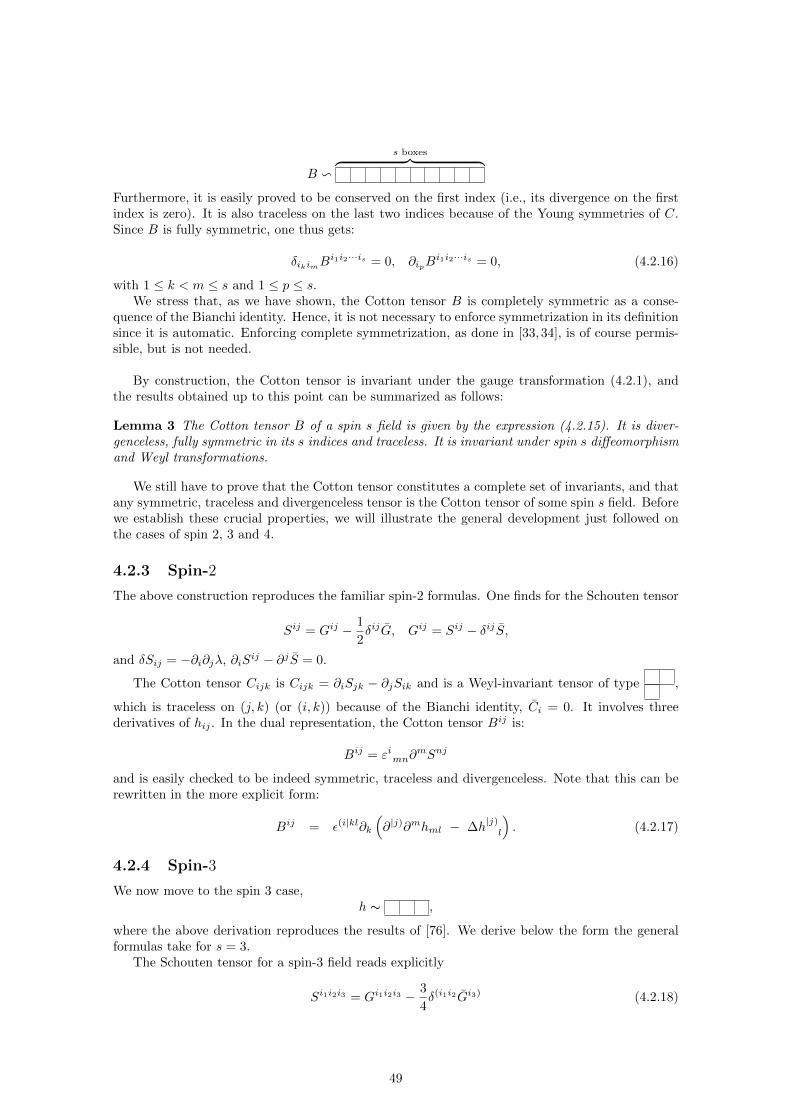
B v

s boxes︷ ︸︸ ︷Furthermore, it is easily proved to be conserved on the first index (i.e., its divergence on the firstindex is zero). It is also traceless on the last two indices because of the Young symmetries of C.Since B is fully symmetric, one thus gets:

δikimBi1i2···is = 0, ∂ipB

i1i2···is = 0, (4.2.16)

with 1 ≤ k < m ≤ s and 1 ≤ p ≤ s.We stress that, as we have shown, the Cotton tensor B is completely symmetric as a conse-

quence of the Bianchi identity. Hence, it is not necessary to enforce symmetrization in its definitionsince it is automatic. Enforcing complete symmetrization, as done in [33, 34], is of course permis-sible, but is not needed.

By construction, the Cotton tensor is invariant under the gauge transformation (4.2.1), andthe results obtained up to this point can be summarized as follows:

Lemma 3 The Cotton tensor B of a spin s field is given by the expression (4.2.15). It is diver-genceless, fully symmetric in its s indices and traceless. It is invariant under spin s diffeomorphismand Weyl transformations.

We still have to prove that the Cotton tensor constitutes a complete set of invariants, and thatany symmetric, traceless and divergenceless tensor is the Cotton tensor of some spin s field. Beforewe establish these crucial properties, we will illustrate the general development just followed onthe cases of spin 2, 3 and 4.

4.2.3 Spin-2

The above construction reproduces the familiar spin-2 formulas. One finds for the Schouten tensor

Sij = Gij − 1

2δijG, Gij = Sij − δijS,

and δSij = −∂i∂jλ, ∂iSij − ∂jS = 0.

The Cotton tensor Cijk is Cijk = ∂iSjk − ∂jSik and is a Weyl-invariant tensor of type ,

which is traceless on (j, k) (or (i, k)) because of the Bianchi identity, Ci = 0. It involves threederivatives of hij . In the dual representation, the Cotton tensor Bij is:

Bij = εimn∂mSnj

and is easily checked to be indeed symmetric, traceless and divergenceless. Note that this can berewritten in the more explicit form:

Bij = ε(i|kl∂k

(∂|j)∂mhml − ∆h

|j)l

). (4.2.17)

4.2.4 Spin-3

We now move to the spin 3 case,h ∼ ,

where the above derivation reproduces the results of [76]. We derive below the form the generalformulas take for s = 3.

The Schouten tensor for a spin-3 field reads explicitly

Si1i2i3 = Gi1i2i3 − 3

4δ(i1i2Gi3) (4.2.18)

49

Its trace is equal to Si = − 14 Gi so that the inverse formula to (4.2.18) is Gi1i2i3 = Si1i2i3 −

3 δ(i1i2 Si3). The Schouten tensor transforms as

δSi1i2i3 = − 3 ∂(i1∂i2µi3) (4.2.19)

under Weyl transformations, where µi is given by

µi = εijk∂jλk (4.2.20)

and fulfills ∂kµk = 0.

The Bianchi identity implies ∂iSi = 0 and can equivalently be written in terms of Si1i2i3 as

∂i1Si1i2i3 − ∂i2 Si3 − ∂i3 Si2 = 0 (4.2.21)

According to the above general definition, the Cotton tensor C = d2(3)S is explicitly given by

Ci1j1|i2j2|i3 = ∂i1∂i2Sj1j2i3 − ∂j1∂i2Si1j2i3−∂i1∂j2Sj1i2i3 + ∂j1∂j2Si1i2i3

and has Young symmetry type:

C v .

In the dual representation, the Cotton tensor Bk1k2k3 reads

Bk1k2k3 = εk1i1j1εk2i2j2∂i1∂i2Sk3

j1j2(4.2.22)

and, using the Bianchi identity (4.2.21) and its consequence ∂jSj = 0, is easily seen to be equal to

Bk1k2k3 = 3∂(i1∂i2 Si3) −∆Si1i2i3 (4.2.23)

an expression that is manifestly symmetric. Transverseness and tracelessness follow again from theBianchi identity (4.2.21).

4.2.5 Spin-4

We now write the formulas in the spin-4 case. The Schouten tensor is

Si1i2i3i4 = Gi1i2i3i4 − δ(i1i2Gi3i4) +1

8δ(i1i2δi3i4) ¯G (4.2.24)

and transforms asδSi1i2i3i4 = − 6 ∂(i1∂i2νi3i4) (4.2.25)

under Weyl transformations, with νij = µij − 16 δij µ.

In terms of the Schouten tensor, the Bianchi identity reads

∂i1Si1i2i3i4 − ∂i2 Si3i4 − ∂i3 Si2i4 − ∂i4 Si2i3 = 0 (4.2.26)

and one has ∂iνij + 1

3∂j ν = 0.

The spin-4 Weyl invariant Cotton tensor is d3(4)S. Writing the explicit formulas directly in the

dual representation, one finds

Bk1k2k3k4 = εk1i1j1εk2i2j2εk3i3j3∂i1∂i2∂i3Sk4

j1j2j3. (4.2.27)

Again, the symmetry in (k1, k2, k3) is manifest, while the symmetry in the last index k4 with anyother index is a consequence of the Bianchi identity (4.2.26). The Cotton tensor is transverse andtraceless,

∂iBijkl = 0, Bij = 0. (4.2.28)

50

4.3 Cotton tensor as a complete set of Weyl invariants

The Cotton tensor is quite important because it is not only gauge invariant, but it also completelycaptures higher spin Weyl invariance. By this, we mean that any function of the higher spin fieldand its derivatives that is invariant under higher spin diffeomorphisms and Weyl transformationsis necessarily a function of the Cotton tensor and its derivatives,

δξ,λf([h]) = 0 ⇒ f = f([B]). (4.3.1)

Equivalently, a necessary and sufficient condition for a spin-s field to be pure gauge (equal tozero up to spin-s diffeomorphisms and Weyl transformations) is that its Cotton tensor vanishes.

The first version of this property is demonstrated in Appendix 4.B. We show here how to provethe second version10:

Lemma 4 A necessary and sufficient condition of a spin-s field to be pure gauge (with the gaugesymmetry (4.2.1)) is that its Cotton tensor vanish.

Assume, then, that the Cotton tensor B (or equivalently, C) is equal to zero. Using thecohomological theorem 1 of Appendix 4.A11, one gets:

C = ds−1(s) S = 0⇒ S = −d2

(s)ν (4.3.2)

for some ν. The Bianchi identity implies that one can choose ν in such a way that the correspondingtensor µ fulfills ∂i1µ

i3···is = 0 and so, can be written as in (4.2.4) for some completely symmetricλk3···ks . This implies in turn that R[h− λ ? δ] = 0, or equivalently ds(s)(h− λ ? δ) = 0. Here, λ ? δstands for the Weyl transformation term δ(i1i2λi3···is). Using again the cohomological theorem 1of Appendix 4.A12, one finally obtains:

h = d(s)ξ + λ ? δ, (4.3.3)

i.e., h is pure gauge. Conversely, if h is pure gauge, the Cotton tensor vanishes. We can thusconclude that a necessary and sufficient condition for the spin-s field to be pure gauge is that itsCotton tensor vanishes.

We illustrate explicitly the derivations in the spin-3 and spin-4 cases.

4.3.1 Spin 3

Consider a spin-3 field hi1i2i3 with vanishing Cotton tensor. According to the theorem 1 of Ap-pendix 4.A13, the Schouten tensor reads

Si1i2i3 = −∂(i1∂i2µi3) (4.3.4)

for some µi. We want to prove that µi can be chosen so that ∂iµi = 0. From the Bianchi identity,

one gets

∂i∂j(∂kµk) = 0

It follows that ∂kµk is at most linear in the coordinates,

∂kµk = a+ bkx

k

Define µk = 13ax

k+ 12ckijx

ixj where ckij = ckji, c(kij) = 0 and ckkj = bj . [Such a ckij exists. It has

the Young symmetry in the dual conventions where symmetry is manifest while antisymmetry

is not. The trace of such a tensor is unconstrained and so can be taken to be equal to bj .] By

10We were kindly informed by Xavier Bekaert that the property “Cotton tensor = 0 ⇔ spin-s field is diffeomor-phism and Weyl pure gauge” can also be viewed as a consequence as the cohomological theorems of [206] on therepresentations of the conformal group, see [22,23]. We are grateful to him for this information.

11See [96,97].12See [96,97].13See [96,97].

51

construction, ∂kµk = ∂kµ

k and ∂(i1∂i2 µi3) = 0, so that Si1i2i3 = −∂(i1∂i2(µi3) − µi3)), implying

that we can assume that µk in (4.3.4) fulfills ∂kµk = 0, which will be done from now on. We then

have µk = εkij∂iλj for some λj , and so the Einstein tensor of hijk is equal to the Einstein tensor of3 δ(ijλk), implying hijk = 3 ∂(iξjk) + 3 δ(ijλk) for some ξi, as announced in the general discussionabove.

4.3.2 Spin 4

We now illustrate the produre for the spin-4 field. The vanishing of the Cotton tensor impliesagain (theorem 1 of Appendix 4.A14),

Si1i2i3i4 = −∂(i1∂i2νi3i4) (4.3.5)

for some νi3i4 . The Bianchi identity yields then

∂(i∂jNk) = 0, Nk ≡ ∂mνkm +1

3∂kν. (4.3.6)

This does not imply that Nk = 0 since, as for spin-3, there are non trivial solutions of the equation∂(i∂jNk) = 0. These solutions have been analyzed in section 6 of [98]. The space of solutions isfinite-dimensional; one easily gets from the equation that the third derivatives of Nk vanish, sothat Nk is at most quadratic in the xi’s,

Nk = ak + bk|mxm + ck|mnx

mxn,

for some constants ak, bk|m and ck|mn = ck|nm which have the respective symmetry , ⊗ ,and ⊗ . Now, let

νkm = ρ(akxm + amxk) + σkm|rsxrxs + θkm|rspx

rxsxp

where the constants ρ, σkm|rs (with symmetry ⊗ ) and θkm|rsp (with symmetry ⊗) are chosen such that (i) σ(km|ij) = 0, θ(km|ij)p = 0 so that ∂(i∂j νkm) = 0; and (ii)

Nk = Nk. This is always possible since this second condition restricts only the traces, which areleft free by the first condition. Then, by substracting νkm from νkm, one sees that one can assumeNk = 0. This implies that the corresponding µkm can be assumed to fulfill ∂mµ

km = 0 and thusis equal to µkm = εkrsεmpq∂r∂pλsq for some λsq = λqs. Therefore, the Einstein tensor of hijkm isequal to the Einstein tensor of δ(ijλkm), implying that

hijkm = 4 ∂(iξjkm) + 6 δ(ijλkm),

which is the result that we wanted to prove.

4.4 Cotton tensors as a complete set of transverse-tracelesssymmetric tensors

We have proven so far the vanishing of its Cotton tensor was a necessary and sufficient conditionfor a spin-s field to be conformally flat. Let us now establish that a tensor that has the propertiesof the Cotton tensor is the Cotton tensor of an existing field:

Lemma 5 For any symmetric, divergenceless and traceless tensor B with s indices, there exists asymmetric tensor of same rank of which B is the Cotton tensor.

4.4.1 The problem

We have recalled with corollary 2 of section 4.1.2 that if a completely symmetric tensor Gi1···is

fulfills the equation∂i1G

i1i2···is = 0, (4.4.1)

14See [96,97].

52

then there exists hi1···is such that G = G[h].We want to address the question: let Bi1i2···is be a completely symmetric tensor that is both

transverse∂i1B

i1i2···is = 0, (4.4.2)

and traceless,δi1i2B

i1i2i3···is = 0, (4.4.3)

Does there exist a totally symmetric tensor Zi1···is such that Bi1i2···is is the Cotton tensor ofZi1···is?

We prove here that the answer is affirmative, starting with the spin-2 case.

4.4.2 Spin 2

The Cotton tensor Bij is dual to Cijk = −Cjik on the first index. The tracelessness condition on

Bij implies that Cijk has Young symmetry type , while the symmetry in (i, j) of Bij implies

that Cijk is traceless. The divergenceless condition on Bij implies then, by Poincare lemma (kbeing a “spectator” index) that

Cijk = ∂iSjk − ∂jSik (4.4.4)

where Sik is not a priori symmetric. However, the ambiguity in Sik is Sik → Sik + ∂iTk, andusing this ambiguity, the condition C[ijk] = 0 and Poincare lemma, one easily sees that Sik can beassumed to be symmetric. Then, the tracelessness condition implies the Bianchi identity ∂iS

ij −∂jS = 0 for Sij (or ∂iG

ij = 0 for Gij), from which follows the existence of Zij such that S = S[Z]and thus B = B[Z]. This establishes the result.

4.4.3 Higher spin

The same steps work for higher spins. For instance, for spin 3, the reasoning proceeds as follows:

• Define Ci1j1|i2j2|k from Bijk by dualizing on the first two indices, with k “spectator”,

Ci1j1|i2j2|k = εi1i2iεj1j2jδkmBijm (4.4.5)

• Because Bijm is completely symmetric and traceless, Ci1i2|j1j2|k has Young symmetry type

and is traceless on k and any other of its indices.

• The transverse condition on Bijk is equivalent to d(2)C = 0 where d(2) is acting on C as if

it was a collection of tensors of type parametrized by k. The Poincare lemma implies

then the existence of a tensor Rijk such that

Ci1j1|i2j2|k = ∂[i1∂[j1Ri2]j2]k (4.4.6)

where the antisymmetrizations are on the pairs of indices (i1, i2) and (j1, j2). At this stage,the tensor R has a component S that is completely symmetric S ∼ ,

Si2j2k =1

3(Ri2j2k +Rj2ki2 +Rki2j2) (4.4.7)

= S(i2j2k) (4.4.8)

and a component T that has Young symmetry type ,

Tijk = Tkji − Tkij (4.4.9)

3Tkji = Tijk + Tikj (4.4.10)

withTi2j2k = 2Ri2j2k −Rkj2i2 −Rki2j2 (4.4.11)

53

Explicitly,

Ri2j2k = Si2j2k +1

3Ti2j2k. (4.4.12)

The change from T to T corresponds to the change of conventions in which either antisym-metry or symmetry is manifest. We shall call T the “Curtright tensor”.

• The tensor Ri2j2k is not completely determined by Ci1j1|i2j2|k since one may add to it

Ri2j2k → Ri2j2k + ∂i2µj2k + ∂j2µi2k (4.4.13)

without violating (4.4.6). This is the only ambiguity.

• Furthermore, the condition Ci1j1|[i2j2|k] = 0 is easily verified to imply that the strength fieldof the Curtright tensor is equal to zero, so that T is pure gauge and can be set equal to zeroby a gauge transformation of the type (4.4.13). Therefore, one can assume

Ci1j1|i2j2|k = ∂[i1∂[j1Si2]j2]k (4.4.14)

with S completely symmetric.

• The residual gauge symmetry after T has been set equal to zero is given by

Sijk → Sijk + ∂(i∂jµk) (4.4.15)

(which is still present because the gauge symmetries of the Curtright tensor are reducible).

• Finally, the tracelessness condition of C on k and any other index yields

∂[i1Ui2]j = 0 (4.4.16)

whereUij = ∂kSijk − ∂iSj − ∂jSi (4.4.17)

is such that Uij = 0 is the Bianchi identity for the Schouten tensor (see (4.2.21)). Now,(4.4.16) implies

Uij = ∂i∂jρ (4.4.18)

for some ρ ( cohomology of d(2) for d(2) with d3(2) = 0). On the other hand, Uij transforms as

Uij → Uij − 3∂i∂j(∂kµk) (4.4.19)

under (4.4.15). This enables one to chose S to obey the Bianchi identity of the Schoutentensor (take µk such that 3∂kµ

k = ρ), implying the existence of Zijk such that S = S[Z]and hence B = B[Z]. [Note that δU = 0 when ∂kµ

k = 0, as it should.] This ends thedemonstration of the property that we wanted to prove.

54

Appendix

4.A Generalized differential

4.A.1 p-forms

If we consider tensor fields over a flat manifold of dimension D - on which ordinary partial deriva-tives provide us with a satisfactory connection, we know that, if we limit ourselves to fully antisym-metric (covariant) tensors (also called p-forms, p being their number of indices), not only can wedefine an internal product over this space (that associates to a p-form and a q-form a (p+ q)-formin an associative way), turning it into a graded Grassmann algebra, but we can also define a uniqueexterior derivative d that send p-forms to (p+ 1)-forms and which satisfies a series of properties(its action on a 0-form, which is a scalar function, gives the gradient of this function; it obeysLeibnitz rule when acting on a product of p-forms; . . . ). It can be explicitly built in the followingway: if ω is a p-form with components ωi1...is

15, its exterior derivative will be the (p+ 1)-form dωwith components given by (dω)i1...ip+1

= (p+ 1) ∂[i1ωi2...ip+1].The most remarkable feature of this differential operator is, of course, that it squares to zero:

d2 = 0. This naturally leads us to look at the cohomology of d, that is, to ask whether there existp-forms annihilated by d which are not themselves the exterior derivative of a (p− 1)-form. Inother words, are there closed p-forms that are not exact ? As is well-known, as long as we considerantisymmetric tensor fields over a manifold which has the topology of RD, the answer turns out tobe negative for forms of non-zero degree (for p = 0, the kernel of d - which is the set of constantfunctions, R - is also the cohomology of d, since 0-forms can not be obtained by taking the exteriorderivative of anything).

The precise notation of the cohomology is the following: Hp (d) is the set of closed p-formsmodulo exact ones. We then have the following result over RD:

0 = Hp (d) for p ≥ 1, (4.A.1)

R = H0 (d) . (4.A.2)

These results are of particular interest when one considers the spin 1 massless field, the photon,whose potential is a one-form A (that is, a vector field). Its curvature is the strength field two-formF which is the exterior derivative of the potential: F ≡ dA. Since the physically observable objectis the strength field, one easily identifies the gauge invariance of the potential as the kernel of d ofform degree one, which, thanks to the absence of cohomology, is the set of exact one-forms, or theset of external derivative of zero-form. In other words, a gauge variation of the potential is givenby δA = df , f being a scalar function.

In addition, a necessary and sufficient condition for a two-form F to be the strength field tensorof a potential is that its exterior derivative should vanish, dF = 0⇔ ∃A such that F = dA.

4.A.2 Beyond fully antisymmetric tensors

The construction outlined above applies to fully antisymmetric tensors, whose Young diagramconsists of a single column. We are now going to give the results of interest concerning thegeneralization of the concept of exterior derivative to tensors of more complex symmetry16.

15Which means that in the corresponding base of 1-forms ei, we have ω = ωi1...isei1⊗. . .⊗

eip .16These tools have been introduced in [97,98]. See also [25,187] for a general discussion of cohomological techniques

adapted to tensor fields with mixed Young symmetry of general type.

55

In full generality, one should consider an arbitrary sequence of Young diagrams Y p, p being apositive integer and the number of boxes of Y p. The exterior derivative would send tensor fields ofsymmetry given by Y p to tensor fields of symmetry given by Y p+1. However, we do not need suchan elaborate construction, and we will limit ourselves to the following type of sequence: we will onlyconsider Young diagrams with a maximal number of columns, say N . In addition, we will requirethese Young diagrams to have rows with exactly N boxes, except for the last one. In other words,we are interested in Young diagrams of the form (N, . . . , N, l) ≡

(Nk, l

), with 0 ≤ l ≤ N − 1. d

will simply be the composition of the projector on the appropriate Young diagram with the partialderivative.

So, we have in mind tensor fields over RD whose symmetry is given by Young diagrams of thefollowing structure:

N boxes︷ ︸︸ ︷. (4.A.3)

(In the diagram shown above, N = 5, k = 4 and l = 3).We can then arrange these diagrams in a sequence Y pN , p being the number of boxes (equiva-

lently, Y pN ≡(Nk, l

), where p = Nk + l, with 0 ≤ k and 0 ≤ l ≤ N − 1). If we denote by Yp

N theprojector of tensors with p indices on the space of tensors whose symmetry is given by the Youngdiagram Y pN , our external derivative is given by:

d(N) ≡ Yp+1N ∂ : Y pN → Y p+1

N . (4.A.4)

The set of tensor fields over RD of symmetry type Y pN for any p (for a given N) will be denotedby ΩN

(RD). We defined an internal derivative acting on it, and we could easily define an internal

product over it, turning it into a graded (by p) Grassmann algebra. It is also called a differentialN -complex, for reasons that we are going to explain.

Since partial derivatives commute and indices are antisymmetrized in each column, and wehave no more than N columns, taking N+1 times the generalized exterior derivative d must resultin the antisymmetrization of two partial derivatives, giving zero. So, we have:

0 = dN+1(N) . (4.A.5)

As before, this suggests to consider cohomologies. We would like to find Hp(k)

(ΩN

(RD), d(N)

),

which is the set of tensor fields of symmetry type Y pN annihilated by dk(N) modulo those which are

the image of tensor fields of symmetry type Y p+k−N−1n through the action of dN+1−k

(N) .

Contrarily to the simple N = 1 case of the p-forms, which was developed above, this cohomologyis not generally empty for non zero p. However, it is empty as long as we consider well-filled tensors,whose Young diagram is rectangular. Equivalently, Hp

(k)

(ΩN

(RD), d(N)

)is empty if N divides p

without rest. Thus, we have the following theorem (whose proof can be carried on through theexplicit construction of the relevant homotopies):

Theorem 1 HmN(k)

(ΩN

(RD), d(N)

)= 0, ∀m ≥ 1.

As for H0(k)

(ΩN

(RD), d(N)

), one can easily convince oneself that it consists solely of the real

polynomials function on RD of degree strictly less than k.

56

4.B Complete set of gauge invariant functions

4.B.1 Generalities

Let ϕA be some fields invariant under some gauge symmetries,

δξϕA = kAα ξ

α + kAiα ∂iξα + kAijα ∂i∂jξ

α (4.B.1)

where for definiteness, we have assumed that the gauge parameters and their derivatives up tosecond order appear in the gauge transformations. The discussion would proceed in the same wayif there were higher derivatives present in (4.B.1). We also assume that the coefficients kAα , kAiαand kAijα do not involve the fields, so that the gauge transformations are of zeroth order in thefields (and of course linear in the gauge parameters).

We consider local functions, i.e., functions f(ϕA, ∂iϕA, · · · , ∂i1∂i2 · · · ∂ikϕA) of the fields and

their derivatives up to some finite but unspecified order. That unspecified order can depend on f .We denote such local funtions as f([ϕA)]). Among the local functions, the gauge invariant onesare particularly important. In our linear theories, non trivial (i.e., not identically constant) localfunctions that are gauge invariant exist. For instance, the components of the (linearized) Riemanntensor are local gauge invariant functions under the (linearized) diffeomorphisms. [Gauge symme-tries that involve the fields might not allow for non trivial local gauge invariant functions. Thisoccurs for example in the case of full diffeomorphism invariance where even the scalar curvature(say) transforms under change of coordinates, δξR = ξi∂iR (transport term).]

The local functions are functions on the “jet spaces” Jk, which can be viewed, in the freetheories investigated here, as the vector spaces with coordinates given by the field componentsϕA and their successive derivatives up to order k. The gauge orbits obtained by integrating thegauge transformations are m-dimensional planes in those vector spaces Jk, where m is the numberof independent gauge parameter components and their derivatives (effectively) appearing in thegauge transformations of the fields and their derivatives up to order k.

For instance, for a free spin 3-field in 3 dimensions, J0 has dimension 10 because there are10 independent undifferentiated field components hijk. The gauge orbits have also dimension 10since there are 18 independent derivatives ∂kξij of the gauge parameters but only 10 of them, thesymmetrized ones ∂(kξij) effectively appear in the gauge transformations. Accordingly, J0 is a singlegauge orbit. Similarly, J1 has dimension 10+30 = 40, the new coordinates being the 30 derivatives∂mhijk of the fields. There are 36 independent second derivatives of the gauge parameters but only30 of them effectively act in the gauge transformations of the ∂mhijk. The jet space J1 reducesagain to a single gauge orbit. This is also true for J2. It is only in the jet spaces Jk with k ≥ 3that the gauge orbits have a dimension strictly smaller than the dimension of the correspondingjet spaces. For J3, which has dimension 10 (number of undifferentiated field components hijk)+30 (number of ∂mhijk) +60 (number of ∂m∂nhijk) +100 (number of ∂m∂n∂qhijk) = 200, thegauge orbits have dimension 10 (number of effective ∂kξij) +30 (number of effective ∂k∂mξij) +60(number of ∂k∂m∂qξij , which are all effective) +90 (number of ∂k∂m∂q∂rξij , which are all effective)= 190. Accordingly, the quotient space of J3 by the 190-dimensional planes generated by the gaugetransformations has dimension 10, which is – as it should – the number of independent componentsof the Riemann tensor, which has Young symmetry

.

Without loss of generality, we can assume that the gauge invariant functions vanish whenthe fields ϕA and their derivatives vanish (just substract from f the gauge invariant constantf(0, 0, · · · , 0)).

A set of gauge invariant functions f∆ is said to form a complete set if any gauge invariantfunction f can be expressed as a function of the f∆, δξf = 0 ⇒ f = f(f∆). There might berelations among the f∆’s (redundancy) but this will not be of concern to us. In the linear theoriesconsidered here, we can construct complete sets of gauge invariant functions that are linear in thefields and their derivatives.

Consider a definite jet space Jk, with k fixed but arbitrary. Let f∆ be a complete set of

gauge invariant functions. The functions f(k)∆ in this complete set that involve derivatives of the

fields up to order k are defined in Jk. They provide a coordinate system of the linear quotient

57

space of Jk by the gauge orbits Ok (in case of redundancy, one must take a subset of independent

f(k)∆ ). If this were not the case, one could find a gauge invariant function in Jk not expressible in

terms of the functions in the complete set. The trivial orbit of the pure gauge field configurationsis the orbit of 0, on which the gauge invariant functions have been adjusted to vanish. It followsfrom these observations that a set f∆ of gauge invariant functions is a complete set if and onlyif the condition f∆ = 0 implies that the fields are pure gauge.

4.B.2 Spin-s Weyl invariance

We now turn to the proof that a complete set of invariants for higher spin conformal fields in threedimensions is given by the Cotton tensor and its successive derivatives. As we just shown, this isequivalent to the statement that the vanishing of the Cotton tensor implies that the spin-s field ispure gauge.

To determine a complete set of invariants, we reformulate the problem as a problem of cohomogyin the successive jet spaces augmented by new fermionic variables, “the ghosts”, and decomposethe successive derivatives in irreducible representations of GL(3). This approach is standard andhas been developed successively in the case of spin-s diffeormorphism invariance for spin 1 [95,11,12,42–44,96,130], spin 2 [39] and spin s [26].

Weyl invariance for spin-2 was treated in [40]. By the same techniques as those developedin that reference, one first takes care of spin-s diffeomorphism invariance and concludes thatdiffeomorphism invariance forces the local functions to be functions of the Riemann tensor and itsderivatives, or, what is the same in D = 3, of the Schouten tensor and its derivatives, f = f([S]).Spin-s Weyl invariance becomes then the condition δνf = 0 for δνSi1···is = −∂(i1i2νi3···is) (for

convenience, we absorb the factor s(s−1)2 in a redefinition of ν). Furthermore, neither the Schouten

tensor nor the gauge parameter ν are independent since their divergences are constrained by(4.2.10) and (4.2.11).

To investigate the problem of Weyl invariance, we shall first consider the problem δνf = 0 forδνSi1···is = −∂(i1i2νi3···is) for unconstrained S and ν. We shall then analyse the implications of theconstraints (4.2.10) and (4.2.11) on the divergences.

We thus consider the problem of computing the cohomology at “ghost number” zero of thedifferential γ defined by

γSi1···is = ∂(i1i2Ci3···is), γCi1···is−2= 0 (4.B.2)

We introduce a derivative degree that gives weight zero to the ghosts and weight two to theSchouten tensor.

At derivative degree 0, we have only the ghosts in the cohomology, but these are at ghostnumber one, so there is no cohomology at ghost number zero. At derivative degree 1, there isagain no cohomology at ghost number zero for a similar reason. The ghost-number-zero variables(Schouten tensor) appear only in derivative degree 2 and higher.

At derivative degree 2, the second derivatives of the ghosts transform in the representation

s− 2 boxes︷ ︸︸ ︷⊗

=

s boxes︷ ︸︸ ︷

⊕

s− 1 boxes︷ ︸︸ ︷

⊕

s− 2 boxes︷ ︸︸ ︷while the undifferentiated Schouten tensor components transform in the representation

s boxes︷ ︸︸ ︷.

58

It follows that the undifferentiated Schouten tensor components form contractible pairs with thederivatives of the ghosts transforming in the same representation and disappear from the cohomol-ogy. There is no cohomology at ghost number zero. The same story proceeds in the same way,with the derivatives of the Schouten tensor being all “eaten” through contractible pairs with thecorresponding derivatives of the ghosts and no cohomology at ghost number zero, with non trivialgenerators at ghost number one left over, up to derivative degree s. There one finds for the ghosts:

s− 2 boxes︷ ︸︸ ︷⊗

s boxes︷ ︸︸ ︷=

2s− 2 boxes︷ ︸︸ ︷

⊕

2s− 3 boxes︷ ︸︸ ︷⊕ · · ·

⊕

s+ 1 boxes︷ ︸︸ ︷

⊕

s boxes︷ ︸︸ ︷(4.B.3)

and exactly the same decomposition for the representation in which the derivatives of order s− 2of the Schouten tensor transform,

s boxes︷ ︸︸ ︷⊗

s− 2 boxes︷ ︸︸ ︷.

There is exact matching and the generators of derivatives order s form contractible pairs and donot contribute to the cohomology.

At higher derivative order, it is now some of the derivatives of the Schouten tensor that areunmatched, namely those which contain the Cotton tensor

s boxes︷ ︸︸ ︷︸ ︷︷ ︸

s− 1 boxes

since these representations (and only those) cannot arise in the decomposition of the derivativesof the ghosts of order t > s

s− 2 boxes︷ ︸︸ ︷⊗

t > s boxes︷ ︸︸ ︷(the lower line can have at most length s− 2 as shown by (4.B.3)).

Accordingly, we can conclude that the γ-cohomology of the differential defined by (4.B.2), withunconstrained variables, is given at ghost number zero by the functions f([C]) of the Cotton tensorand its derivatives.

We did not take into account so far the constraints (4.2.10) and (4.2.11) that the Schoutentensor should obey the Bianchi identity and that the divergence of the ghost is also determinedby its trace. One must verify that the derivatives of the Schouten tensor that were trivial in theγ-cohomology because they had an independent ghost partner equal to their γ-variation, eithervanish on account of the constraints or, if they do not vanish, that their ghost partner in the trivialpair also remains different from zero so that both elements in the trivial pair continue being trivial.

It is easy to convince oneself that this is the case. The derivatives of the Schouten tensorthat remain non-zero after the Bianchi identity has been taken into account may be assumed

59

not to involve a contraction of one derivative index ∂i with an index of the Schouten tensor,since such terms can be eliminated using the Bianchi identity. In fact, once we have eliminatedsuch contractions, the remaining derivatives are unconstrained. A similar situation holds on theghost side. If the γ-variation of a derivative of the Schouten tensor without such contractionsinvolves the ghosts and so is not γ-closed before the constraints are taken into account, it willremain so after the constraints are taken into account because its γ-variation necessarily produceindependent derivatives of the ghosts without such contractions (in addition to possible terms withsuch contractions coming from possible traces).

60

Chapter 5

Hamiltonian analysis

Now equipped with the knowledge we have acquired on higher spin conformal geometry, we areready to make a systematic study of the Hamiltonian dynamics of free massless higher spin fieldsover a flat four dimensional space-time.

Indeed, similarly to what happened with the well-known lower spin cases (which we studiedin section 2.2.1 and 2.2.2), and as can be implied from the general theory of gauge systems (aswe saw in section 2.1.2), we will find out that massless higher spin have a constrained first orderformalism, whose constrains will be solved in a very natural way through the use of conformalcurvatures.

In order to keep the logic visible, we will begin with an extensive study of the spin-3 case,before moving on to the arbitrary spin. The development will be along the same lines in each case:expand Fronsdal action (1.1.13) in order to extract the momenta and compute the Hamiltonianand the constraints; then, check that these are first class (that the constraints generate gaugetransformations, which preserve both the constraints and the Hamiltonian); eventually, solve theconstraints through the introduction of prepotentials in terms of which the Hamiltonian action willbe rewritten.

The more technical features observed in the case of spin one or two (sections 2.2.1 and 2.2.2)will also reappear: the prepotentials will be two spatial symmetric tensors, of the same rank asthe initial field, and they will enjoy a gauge invariance including both diffeomorphism and Weylrescaling.

5.1 Spin-3

Our starting point is the Lagrangian formulation introduced for arbitrary spin in section 1.1.1.The spin-3 field is described by a symmetric covariant tensor field hµνρ with the gauge symmetry:

δhµνρ = 3 ∂(µξνρ), (5.1.1)

where ξµν is a symmetric traceless tensor: ξ′ = 0. The field itself is unconstrained.With such a gauge invariance, we can build the second order gauge invariant curvature (which

is the Fronsdal tensor, defined for any spin in (1.1.3)):

Fµνρ = hµνρ − 3 ∂σ∂(µhνρ)σ + 3 ∂(µ∂νh′ρ). (5.1.2)

The equations of motion of the spin-3 are the vanishing of this tensor, and they can be seen tofollow from the following gauge invariant action (introduced for an arbitrary spin in (1.1.15)):

S = − 1

2

∫d4x ∂σhµνρ∂σhµνρ − 3 ∂σhσµν∂ρh

ρµν + 6 ∂ρhρµν∂µh′ν

− 3 ∂µh′ν∂

µh′ν − 3

2∂νh′ν∂µh

′µ. (5.1.3)

61

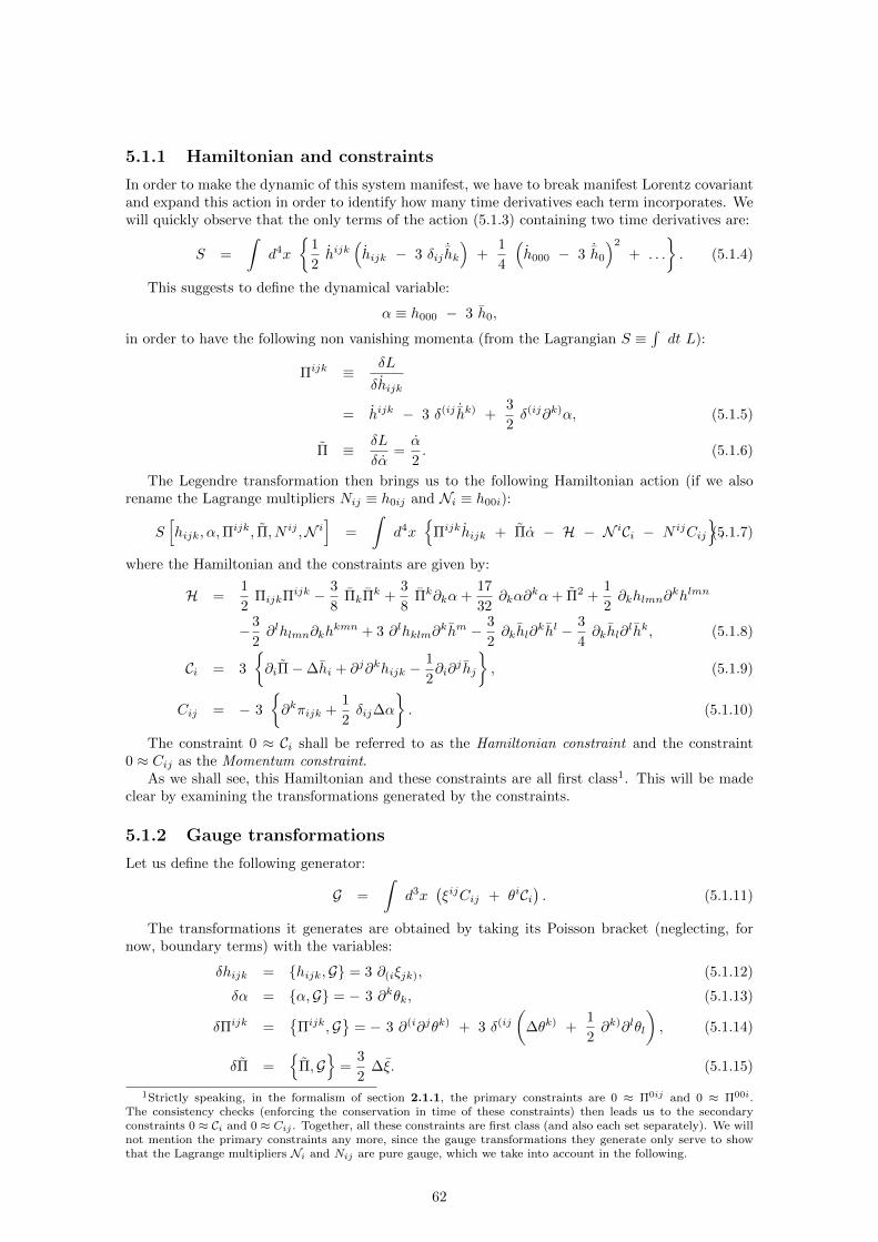
5.1.1 Hamiltonian and constraints

In order to make the dynamic of this system manifest, we have to break manifest Lorentz covariantand expand this action in order to identify how many time derivatives each term incorporates. Wewill quickly observe that the only terms of the action (5.1.3) containing two time derivatives are:

S =

∫d4x

1

2hijk

(hijk − 3 δij

˙hk

)+

1

4

(h000 − 3 ˙h0

)2

+ . . .

. (5.1.4)

This suggests to define the dynamical variable:

α ≡ h000 − 3 h0,

in order to have the following non vanishing momenta (from the Lagrangian S ≡∫dt L):

Πijk ≡ δL

δhijk

= hijk − 3 δ(ij ˙hk) +3

2δ(ij∂k)α, (5.1.5)

Π ≡ δL

δα=α

2. (5.1.6)

The Legendre transformation then brings us to the following Hamiltonian action (if we alsorename the Lagrange multipliers Nij ≡ h0ij and Ni ≡ h00i):

S[hijk, α,Π

ijk, Π, N ij ,N i]

=

∫d4x

Πijkhijk + Πα − H − N iCi − N ijCij

,(5.1.7)

where the Hamiltonian and the constraints are given by:

H =1

2ΠijkΠijk − 3

8ΠkΠk +

3

8Πk∂kα+

17

32∂kα∂

kα+ Π2 +1

2∂khlmn∂

khlmn

−3

2∂lhlmn∂kh

kmn + 3 ∂lhklm∂khm − 3

2∂khl∂

khl − 3

4∂khl∂

lhk, (5.1.8)

Ci = 3

∂iΠ−∆hi + ∂j∂khijk −

1

2∂i∂

j hj

, (5.1.9)

Cij = − 3

∂kπijk +

1

2δij∆α

. (5.1.10)

The constraint 0 ≈ Ci shall be referred to as the Hamiltonian constraint and the constraint0 ≈ Cij as the Momentum constraint.

As we shall see, this Hamiltonian and these constraints are all first class1. This will be madeclear by examining the transformations generated by the constraints.

5.1.2 Gauge transformations

Let us define the following generator:

G =

∫d3x

(ξijCij + θiCi

). (5.1.11)

The transformations it generates are obtained by taking its Poisson bracket (neglecting, fornow, boundary terms) with the variables:

δhijk = hijk,G = 3 ∂(iξjk), (5.1.12)

δα = α,G = − 3 ∂kθk, (5.1.13)

δΠijk =

Πijk,G

= − 3 ∂(i∂jθk) + 3 δ(ij

(∆θk) +

1

2∂k)∂lθl

), (5.1.14)

δΠ =

Π,G

=3

2∆ξ. (5.1.15)

1Strictly speaking, in the formalism of section 2.1.1, the primary constraints are 0 ≈ Π0ij and 0 ≈ Π00i.The consistency checks (enforcing the conservation in time of these constraints) then leads us to the secondaryconstraints 0 ≈ Ci and 0 ≈ Cij . Together, all these constraints are first class (and also each set separately). We willnot mention the primary constraints any more, since the gauge transformations they generate only serve to showthat the Lagrange multipliers Ni and Nij are pure gauge, which we take into account in the following.

62

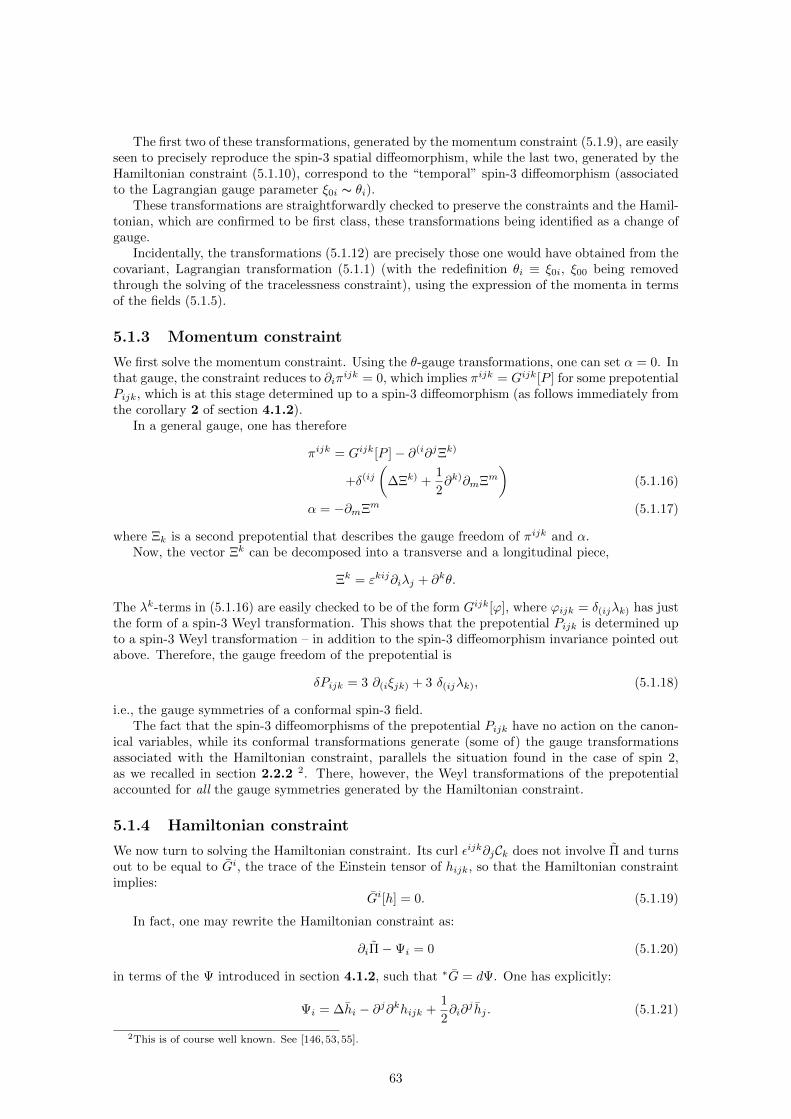
The first two of these transformations, generated by the momentum constraint (5.1.9), are easilyseen to precisely reproduce the spin-3 spatial diffeomorphism, while the last two, generated by theHamiltonian constraint (5.1.10), correspond to the “temporal” spin-3 diffeomorphism (associatedto the Lagrangian gauge parameter ξ0i ∼ θi).

These transformations are straightforwardly checked to preserve the constraints and the Hamil-tonian, which are confirmed to be first class, these transformations being identified as a change ofgauge.

Incidentally, the transformations (5.1.12) are precisely those one would have obtained from thecovariant, Lagrangian transformation (5.1.1) (with the redefinition θi ≡ ξ0i, ξ00 being removedthrough the solving of the tracelessness constraint), using the expression of the momenta in termsof the fields (5.1.5).

5.1.3 Momentum constraint

We first solve the momentum constraint. Using the θ-gauge transformations, one can set α = 0. Inthat gauge, the constraint reduces to ∂iπ

ijk = 0, which implies πijk = Gijk[P ] for some prepotentialPijk, which is at this stage determined up to a spin-3 diffeomorphism (as follows immediately fromthe corollary 2 of section 4.1.2).

In a general gauge, one has therefore

πijk = Gijk[P ]− ∂(i∂jΞk)

+δ(ij

(∆Ξk) +

1

2∂k)∂mΞm

)(5.1.16)

α = −∂mΞm (5.1.17)

where Ξk is a second prepotential that describes the gauge freedom of πijk and α.Now, the vector Ξk can be decomposed into a transverse and a longitudinal piece,

Ξk = εkij∂iλj + ∂kθ.

The λk-terms in (5.1.16) are easily checked to be of the form Gijk[ϕ], where ϕijk = δ(ijλk) has justthe form of a spin-3 Weyl transformation. This shows that the prepotential Pijk is determined upto a spin-3 Weyl transformation – in addition to the spin-3 diffeomorphism invariance pointed outabove. Therefore, the gauge freedom of the prepotential is

δPijk = 3 ∂(iξjk) + 3 δ(ijλk), (5.1.18)

i.e., the gauge symmetries of a conformal spin-3 field.The fact that the spin-3 diffeomorphisms of the prepotential Pijk have no action on the canon-

ical variables, while its conformal transformations generate (some of) the gauge transformationsassociated with the Hamiltonian constraint, parallels the situation found in the case of spin 2,as we recalled in section 2.2.2 2. There, however, the Weyl transformations of the prepotentialaccounted for all the gauge symmetries generated by the Hamiltonian constraint.

5.1.4 Hamiltonian constraint

We now turn to solving the Hamiltonian constraint. Its curl εijk∂jCk does not involve Π and turnsout to be equal to Gi, the trace of the Einstein tensor of hijk, so that the Hamiltonian constraintimplies:

Gi[h] = 0. (5.1.19)

In fact, one may rewrite the Hamiltonian constraint as:

∂iΠ−Ψi = 0 (5.1.20)

in terms of the Ψ introduced in section 4.1.2, such that ∗G = dΨ. One has explicitly:

Ψi = ∆hi − ∂j∂khijk +1

2∂i∂

j hj . (5.1.21)

2This is of course well known. See [146,53,55].

63

Therefore, the equations Gi = 0 ⇔ dΨ = 0 and dΠ − Ψ = 0 are two equivalent versions of theHamiltonian constraint3.

The form Gi = 0 is more amenable to solution because it falls precisely under the lemma 5of section 4.4. According to what we proved in section 4.4, it implies the existence of a (second)prepotential Φijk such that the Einstein tensor of h is the Cotton tensor of that prepotential,

Gijk[h] = Bijk[Φ]. (5.1.22)

A particular solution of (5.1.22) is given by

hijk = −∆Φijk +3

4δ(ij4Φk)

−3

4δ(ij∂

r∂sΦk)rs +3

10δ(ij∂k)∂

rΦr. (5.1.23)

The last term in (5.1.23) is not necessary but included so that δhijk = 0 under Weyl transfor-mation of Φ.

Now, what are the ambiguities? It is clear that the spin-3 field hijk is determined by (5.1.22) upto a spin-3 diffeomorphism, so that the general solution of (5.1.22) is given by (5.1.23) plus ∂(iujk)

where ujk may be thought of as another prepotential that drops out because of gauge invariance.Conversely, the prepotential Φijk itself is determined by (5.1.22), i.e., by its Cotton tensor, up toa diffeomorphism and a Weyl rescaling,

δΦijk = 3 ∂(iξ′jk) + 3 δ(ijλ

′k) (5.1.24)

with independent gauge parameters ξ′ij and λ′j . Thus, we see that the resolution of the Hamiltonianconstraints also introduces a prepotential possessing the gauge symmetries of a conformal spin-3field. Note that we have adjusted the ambiguity in the dependence of hijk on Φijk in such a waythat the conformal spin-3 transformations of the prepotential leave hijk invariant, while the spin-3diffeomorphisms of the prepotential induce particular spin-3 diffeomorphisms of hijk, as is the casefor spin 2 [146,53,55].

Once hijk is determined, one may work one’s way up to the constraint and solve for Π in termsof the prepotential. One finds

Π = − 1

8∂i∂j∂kΦijk +

3

404∂iΦi (5.1.25)

The use of conformal techniques to solve the Hamiltonian constraint is somewhat reminiscentof the approach to the initial value problem for full general relativity developed in [10,80,231].

5.1.5 Hamiltonian action in terms of prepotentials

When their expressions in terms of the prepotentials is substituted for the fields and the momenta,the Hamiltonian action (5.1.7) takes the following form:

S =1

2

∫d4x

εabZ

aijkB

bijk − δab

(GaijkGbijk −

3

4GaiGbi

), (5.1.26)

where the prepotentials were gathered into a two-vector (Zaijk) ≡ (Pijk,Φijk) (a = 1, 2) and εaband δab are respectively the Levi-Civita tensor and the Euclidean metric in the internal plane ofthe two prepotentials, while Gaijk ≡ Gijk[Za] and Baijk ≡ Bijk[Za]. In terms of the prepotentials,

the action possesses exactly the same structure as the action for spin 2 (2.2.36) 4.The kinetic term in the action is manifestly invariant under the gauge symmetries of the pre-

potentials. The Hamiltonian is manifestly invariant under the spin-3 diffeomorphisms, since itinvolves the Einstein tensors of the prepotentials. It is also invariant under spin-3 Weyl transfor-mations up to a surface term, as it can easily be verified.

3Let us rephrase the argument, in order to be perfectly clear: the vanishing of the trace of the Einstein tensor ofh is equivalent to the vanishing of dΨ. Because of the absence of cohomology, this is equivalent to Ψ being exact,that is, equal to dΠ for some scalar Π - which is precisely what the Hamiltonian constraint requires.

4This expression was, as we said, originally obtained in [53]

64

In terms of the prepotentials, the equations of motion read

Baijk = εabεilm∂lB m

b jk (5.1.27)

and equate the time derivative of the Cotton tensor of one prepotential to the “curl” of the Cottontensor of the other (defined as the right-hand side of (5.1.27)).

5.2 Arbitrary spin

Again, our starting point is the Lagrangian formulation introduced for arbitrary spin in section1.1.1. The spin-s field is described by a symmetric covariant tensor field hµ1···µs

with the gaugesymmetry:

δhµ1···µs= s ∂(µ1

ξµ2···µs), (5.2.1)

where ξµ1···µsis a symmetric traceless tensor: ξ′µ3···µs

= 0. The field itself is subjected to theconstraint that its double trace vanish: h′′µ5···µs

= 0.The equations of motion of the spin-s are the vanishing of its Fronsdal tensor (1.1.3), and they

can be seen to follow from the following gauge invariant action (this is exactly (1.1.15)):

S = − 1

2

∫d4x ∂νhµ1···µs∂

νhµ1···µs − s ∂νhνµ2···µs∂ρhρµ2···µs

+ s (s− 1) ∂νhνρµ3···µs∂ρh′µ3···µs − s (s− 1)

2∂ρh′µ3···µs

∂ρh′µ3···µs

− s (s− 1) (s− 2)

4∂νh′νµ4···µs

∂ρh′ρµ4···µs

. (5.2.2)

5.2.1 Change of variables and momenta

We have to break explicit Lorentz invariance and expand this action, to obtain its Hamiltonianformalism. In order to do that, one has to solve the double-trace constraint on the field h; one canchoose e.g. to encode the independent components of the spin-s field in the traceful spatial tensorshi1···is , h0i2···is , h00i3···is and h000i4···is . The remaining components of the field are dependent onthose and are recursively checked to be equal:

h0...0k2n+1...ks = n h[n−1]00k2n+1...ks

− (n− 1) h[n]k2n+1...ks

,

h0...0k2n+2...ks = n h[n−1]000k2n+2...ks

− (n− 1) h[n]0k2n+2...ks

. (5.2.3)

Within this set one has to distinguish between canonical variables - having conjugate momentasuch that the Legendre transformation is invertible - and Lagrange multipliers. Comparison withwhat happened for the spin 3 and the observation that combinations whose gauge variation (5.2.2)does not contain time derivatives are canonical variables leads to the conclusion that these are thespatial components hi1···is of the field and:

αi4···is ≡ h000i4···is − 3 h0i4···is . (5.2.4)

The remaining independent components of the covariant field are Lagrange multipliers (seetheir gauge transformations in (5.2.13) and (5.2.14)). We denote them as

Ni2···is ≡ h0i2···is , (5.2.5)

Ni3···is ≡ h00i3···is . (5.2.6)

The expansion of the action (5.2.2) confirms our choice of variables, the time derivatives of theLagrange multipliers indeed being absent. The non vanishing momenta are (with the Lagrangian

65

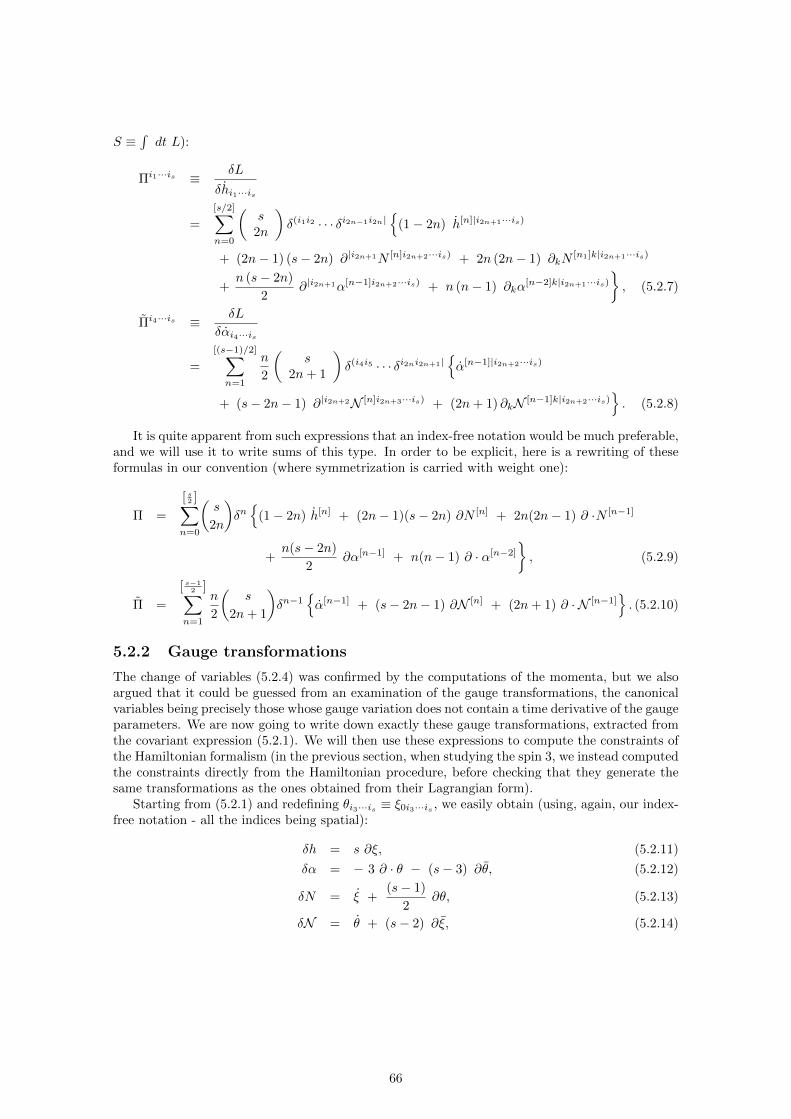
S ≡∫dt L):

Πi1···is ≡ δL

δhi1···is

=

[s/2]∑n=0

(s

2n

)δ(i1i2 · · · δi2n−1i2n|

(1− 2n) h[n]|i2n+1···is)

+ (2n− 1) (s− 2n) ∂|i2n+1N [n]i2n+2···is) + 2n (2n− 1) ∂kN[n1]k|i2n+1···is)

+n (s− 2n)

2∂|i2n+1α[n−1]i2n+2···is) + n (n− 1) ∂kα

[n−2]k|i2n+1···is)

, (5.2.7)

Πi4···is ≡ δL

δαi4···is

=

[(s−1)/2]∑n=1

n

2

(s

2n+ 1

)δ(i4i5 · · · δi2ni2n+1|

α[n−1]|i2n+2···is)

+ (s− 2n− 1) ∂|i2n+2N [n]i2n+3···is) + (2n+ 1) ∂kN [n−1]k|i2n+2···is). (5.2.8)

It is quite apparent from such expressions that an index-free notation would be much preferable,and we will use it to write sums of this type. In order to be explicit, here is a rewriting of theseformulas in our convention (where symmetrization is carried with weight one):

Π =

[ s2 ]∑

n=0

(s

2n

)δn

(1− 2n) h[n] + (2n− 1)(s− 2n) ∂N [n] + 2n(2n− 1) ∂ ·N [n−1]

+n(s− 2n)

2∂α[n−1] + n(n− 1) ∂ · α[n−2]

, (5.2.9)

Π =

[ s−12 ]∑

n=1

n

2

(s

2n+ 1

)δn−1

α[n−1] + (s− 2n− 1) ∂N [n] + (2n+ 1) ∂ · N [n−1]

. (5.2.10)

5.2.2 Gauge transformations

The change of variables (5.2.4) was confirmed by the computations of the momenta, but we alsoargued that it could be guessed from an examination of the gauge transformations, the canonicalvariables being precisely those whose gauge variation does not contain a time derivative of the gaugeparameters. We are now going to write down exactly these gauge transformations, extracted fromthe covariant expression (5.2.1). We will then use these expressions to compute the constraints ofthe Hamiltonian formalism (in the previous section, when studying the spin 3, we instead computedthe constraints directly from the Hamiltonian procedure, before checking that they generate thesame transformations as the ones obtained from their Lagrangian form).

Starting from (5.2.1) and redefining θi3···is ≡ ξ0i3···is , we easily obtain (using, again, our index-free notation - all the indices being spatial):

δh = s ∂ξ, (5.2.11)

δα = − 3 ∂ · θ − (s− 3) ∂θ, (5.2.12)

δN = ξ +(s− 1)

2∂θ, (5.2.13)

δN = θ + (s− 2) ∂ξ, (5.2.14)

66

and, using the expression of the momenta in terms of the fields (5.2.7) and (5.2.8):

δΠ =

[s/2]∑n=0

(s

2n

)δn

(n− 1) (s− 2n) (s− 2n− 1)

2∂2θ[n]

+ n[(n− 1) (2n− 1) ∂ · ∂ · θ[n−2] + n4 θ[n−1]

+(4n− 3) (s− 2n)

2∂∂ · θ[n−1]

], (5.2.15)

δΠ =

[ s−12 ]∑

n=1

n

2

(s

2n+ 1

)δn−1

2 (n− 1) (2n+ 1) ∂ · ∂ · ξ[n−1] + (2n+ 1)4 ξ[n]

+ (s− 2n− 1)[(4n+ 1) ∂∂ · ξ[n] + (s− 2n− 2) ∂2ξ[n+1]

]. (5.2.16)

Note that the parameters ξ and θ appearing in these equations are traceful spatial symmetrictensors with respectively s− 1 and s− 2 indices.

These variations indeed confirm, again, the identification of N and N as the Lagrange multi-pliers.

5.2.3 Hamiltonian and constraints

The Legendre transformation made with the momenta given by (5.2.9) and (5.2.10) on the La-grangian action (5.2.2) will bring it into the Hamiltonian (constrained) form:

S[h, α,Π, Π, N,N

]=

∫d4x

Πh + Πα − H − NC − NC

, (5.2.17)

where the Hamiltonian density H and the constraints C and C only depend on the canonicalvariables.

The variations obtained above from the expression of the momenta (5.2.9)-(5.2.10) and theLagrangian gauge transformations (5.2.1) allow us to directly identify the constraints, withouthaving to compute them explicitly from the Legendre transformation. We will follow this way(and not compute the Hamiltonian either, even though we will later obtain its precise form interms of the prepotentials through invariance arguments).

The gauge transformations must be realized by taking the Poisson bracket of the variables withthe gauge transformations generator, which is precisely the constraints contracted with the gaugeparameters (see section 2.1.2). If we define:

G ≡∫

d3x (ξC + θC) , (5.2.18)

we expect the gauge transformations of the variables to be given by:

δh = h,G =δGδΠ

, (5.2.19)

δα = α,G =δGδΠ

, (5.2.20)

δΠ = Π,G = − δGδh, (5.2.21)

δΠ =

Π,G

= − δGδα. (5.2.22)

The identification of these variations with those computed in the previous section naturally

67

leads to the following expression for the constraints:

C = 3 ∂Π + (s− 3) δ ∂ · Π

−[s/2]∑n=1

n

(s

2n

)δn−1

n h[n] + (n− 2) (2n− 1) ∂ · ∂ · h[n−1]

+(4n− 3) (s− 2n)

2∂∂ · h[n] +

(s− 2n) (s− 2n− 1)

2∂2h[n+1]

, (5.2.23)

C = − s ∂ ·Π

−[ s−1

2 ]∑n=1

n

(s

2n+ 1

)δn

(2n+ 1)

24 α[n−1] + (n− 1) (2n+ 1) ∂ · ∂ · α[n−2]

+(s− 2n− 1) (4n+ 1)

2∂∂ · α[n−1] +

(s− 2n− 1) (s− 2n− 2)

2∂2α[n]

.

(5.2.24)

Let us again draw attention to the fact that each of these expressions is actually a symmetrictensor with s− 2 (for (5.2.23)) or s− 1 indices (for (5.2.24)).

In analogy with the spin 2 case, we will call the constraint (5.2.23) - which is the generator of“temporal” diffeomorphism, given by (5.2.15) - the Hamiltonian constraint, while the constraint(5.2.24) - which is the generator of “spatial” diffeomorphism (5.2.11) - shall be referred to as themomentum constraint.

5.2.4 Solving the momentum constraint

We first solve the momentum constraint (5.2.24). This constraint reads (switching back, for con-venience, to an explicit index notation) :

∂kπki2···is + “more” = 0 (5.2.25)

where “more” stands for terms that are linear in the second order derivatives of αi4···is , whichone can set to zero by a suitable gauge transformation. In the gauges where “more” vanishes, theconstraint reduces to

∂kπki2···is = 0, (5.2.26)

the general solution of which is given by πi1···is = Gi1···is [P ], according to our corollary 2 of section4.1.2. Here Gi1···is [P ] is the Einstein tensor of some prepotential Pi1···is which is totally symmetric.Its explicit expression is given by (4.1.12).

For fixed momentum πi1···is , the prepotential Pi1···is is determined up to a spin-s diffeomor-phism. However, there is a residual gauge freedom in the above gauges, so that πi1···is is notcompletely fixed. It is straightforward but somewhat tedious to check that the residual gauge sym-metry is accounted for by a spin-s Weyl transformation of the prepotential Pi1···is , which thereforeenjoys all the gauge symmetries of a conformal spin-s field.

These results extend what was found earlier for spins 25 (see Section 2.2.2) and 3 6 (see Section5.1.3). It is instructive to exhibit explicitly the formulas in the case of spin 4, which illustrates allthe points and still yields readable expressions.

The momentum constraint reads in this case

0 = 4 ∂nπklmn + 6 δ(kl∆αm)

− 10 δ(kl∂m)∂nαn. (5.2.27)

and the gauge freedom is:

δπklmn = − 12 ∂(k∂lΞmn)

+ 12 δ(kl(∆Ξmn) + ∂m∂

pΞn)p

)+ 4 δ(klδmn)

(2 ∆Ξ + 3 ∂p∂qΞpq

), (5.2.28)

δαk = − 6 ∂lΞkl − 2 ∂kΞ. (5.2.29)

5In [146]6In [132]

68

The residual gauge transformations in the gauge 3 ∆αk − 5 ∂k∂lαl = 0, which eliminates the

α-terms from the constraint, must fulfill

0 = − 18 ∂l∆Ξkl + 4 ∂k∆Ξ + 30 ∂k∂l∂mΞlm.

The divergence of this equation gives (after acting with ∆−1) 3 ∂k∂lΞkl + ∆Ξ = 0. Substitutingthis finding in the previous equation yields, after acting again with ∆−1, 3 ∂l

(Ξkl + 1

3 δklΞ)

= 0.This is the divergence of a symmetric tensor, so the solution is the double divergence of a tensorwith the symmetry of the Riemann tensor:

Ξkl +1

3δklΞ = ∂m∂nΘmknl. (5.2.30)

Therefore, one has

Ξkl = ∂m∂nΘmknl −1

6δkl∂

m∂nΘ npmp . (5.2.31)

This class of gauge transformations can be checked to give a zero variation not only to the contri-bution of αk to the constraint but in fact also to αk itself.

We can dualize Θklmn = εklpεmnqθpq, with a symmetric θkl, to obtain:

Ξkl =5

6δkl(∆θ − ∂m∂nθmn

)+ 2 ∂(k∂

mθl)m − ∂k∂lθ − ∆θkl. (5.2.32)

The gauge transformation of πklmn with this parameter is found then to be exactly the Einsteintensor of a Weyl diffeomorphism

δπklmn = Gklmn[12 δ(pqθrs)

]. (5.2.33)

Once the spin-4 momentum constraint has been brought in the standard form ∂kπklmn = 0 bypartial gauge fixing, it can be solved by the familiar techniques recalled at the beginning of thissection for general s. From the corollary 2 of section 4.1.2, the general solution of the equation∂kπklmn = 0 is indeed the Einstein tensor of a symmetric tensor Pklmn, which is the prepotentialfor the momenta:

πklmn = Gklmn [P ] .

Since the gauge freedom of πklmn is given by the Einstein tensor of a Weyl transformation, thegauge freedom of the prepotential Pklmn will be given by a spin-4 Weyl transformation and a spin-4diffeomorphism:

δPklmn = 4 ∂(kξlmn) + 6 δ(klλmn), (5.2.34)

the first term corresponding to all the transformations of the prepotential leaving πklmn invariantand the second to those realizing on it a residual gauge transformation.

The solution in a general gauge will be given by these expressions to which are added generalgauge transformation terms, parametrized by further prepotentials that drop from the action bygauge invariance and which are usually not considered for that reason.

5.2.5 Solving the Hamiltonian constraint

We now solve the Hamiltonian constraint. The functions Ci2···is are linear in the second orderderivatives of the spin-s field hi1···is and linear in the first order derivatives of the conjugatemomenta Πi4···is . One may rewrite these constraints in the equivalent form (suppressing indices)

Ψ− d(s−2)Π = 0 (5.2.35)

where Ψ is the function of the second order derivatives of the spin-s field with Young symmetry

Ψ ∼

(s−2) boxes︷ ︸︸ ︷,

69

introduced in 4.1.2, such that ∗G ≡∗G[1] = ds−2(s−2)Ψ, where ∗ denotes here the dual on all indices

(on which no trace was taken).The properties of d(s−2) were recalled in 4.A: this differential is nilpotent, ds−1

(s−2) = 0, and

its cohomology is empty when it acts on a symmetric tensor with s − 2 indices, such as Ψ. Thisimplies that the equation (5.2.35) is completely equivalent to ds−2

(s−2)Ψ = 0, i.e., G[1][h] = 0. As we

have recalled, this equation implies in turn the existence of a prepotential Φ for h (continuing toomit indices) such that the Einstein tensor of h is equal to the Cotton tensor of Φ: any symmetric,traceless and divergenceless tensor (a category to which belongs a traceless Einstein tensor) is theCotton tensor of some field - this is our lemma 5 of section 4.4. Once h is expressed in terms ofΦ, the expression ds−2

(s−2)Ψ[Φ] identically vanishes, implying according to the generalized algebraic

Poincare lemma of theorem 1 of Appendix 4.A7 that one can write Ψ[Φ] = d(s−2)Π[Φ], for some

Π[Φ].This completely solves the Hamiltonian constraint in terms of the prepotential Φi1···is . By

construction, this prepotential has the gauge symmetry of a conformal spin-s field.The procedure is direct for spins 1, where there is no Hamiltonian constraint, and 2, where one

gets directly G[1][h] = 0 without having to differentiate. It was detailed for spin 3 in section 5.1.4.It is again instructive to illustrate it explicitly for the spin 4 field, where the formulas remainreadable.

The hamiltonian constraint for the spin 4 is:

Ckl ≡ 3 ∂(kΠl) + δkl∂mΠm

− 6(

∆hkl − ∂m∂nhklmn + ∂(k∂mhl)m + ∂k∂l

¯h)

− 4 δkl∆¯h = 0, (5.2.36)

The gauge freedom of hklmn and Πk is:

δΠk = 6 ∆ξk + 10 ∂k∂lξl, (5.2.37)

δhklmn = 4 ∂(kξlmn). (5.2.38)

One can equivalently rewrite the constraint as

Ckl −1

6δklC ≡ 3 ∂(kΠl) − 6 Ψkl = 0, (5.2.39)

where C is the trace of Ckl and

Ψkl ≡ ∆hkl − ∂m∂nhklmn

+ ∂(k∂mhl)m + ∂k∂l

¯h. (5.2.40)

One has

εkmpεlnq∂m∂nΨpq = Gkl [h] . (5.2.41)

where Gkl is the trace of the Einstein tensor Gklmn [h] of hklmn. So, one gets:

Gkl [h] = − 1

6εkmpεlnq∂

m∂nCpq. (5.2.42)

with Cpq ≡ Cpq − 16 δ

pqC.The Hamiltonian constraint implies Gkl [h] = 0. Therefore, the lemma 5 of section 4.4 yields

Gijkl [h] = Bijkl [Φ] for some prepotential Φklmn, where Bijkl is the Cotton tensor. Explicitly,

hijkl [Φ] = ε(i|mn∂m

[− ∆Φn|jkl) +

1

2δ|jk∆Φnl)

− 1

2δ|jk∂

p∂qΦnl)pq

]+ 4 ∂(iωjkl), (5.2.43)

7See [96,97].

70

where we have added a spin-4 diffeomorphism term parametrized by ωjkl.Direct substitution gives then

Ψij = ∂(i|[3 ∆ωj) + 5 ∂|j)∂

kωk

− 1

8ε|j)mn∂

m(∂k∆Φnk + ∂p∂q∂kΦnkpq

)]. (5.2.44)

from which one derives, using the constraint, the following expression for Πi,

Πi = 6 ∆ωi + 10 ∂i∂kωk

− 1

4εimn∂

m(∂k∆Φnk + ∂p∂q∂kΦnkpq

), (5.2.45)

One could in fact add a solution κi of the equation ∂(iκj) = 0 (Killing equation) to Πi but we do notconsider this possibility here by assuming for instance appropriate boundary conditions (vanishingof all fields at infinity eliminates κi ∼ Ci + µijx

j , where Ci and µij = −µji are constants).

The expression for the spin-s field hi1···is in terms of the prepotential Φi1···is contains s − 1derivatives in order to match the number of derivatives (s) of the Einstein tensor G[h] with thenumber of derivatives (2s − 1) of the Cotton tensor B[Φ]. This number is odd (even) when s iseven (odd) and therefore, in order to match the indices of hi1···is with those of ∂k1 · · · ∂ks−1

Φj1···js ,one needs one εijk when s is even and no εijk when it is odd, together with products of δij ’s.

Even Spins

We first turn to the even s case. We recall that in the spin-2 case, a particular solution is givenby (2.2.30):

hij = ε(i|kl∂kΦl |j). (5.2.46)

The gauge freedom of the prepotential is given by

δΦij = δijσ + 2 ∂(iρj), (5.2.47)

which generates the particular diffeomorphism δhij = ∂(iθj) of the field, where θi = εikl∂kρl (it is a

diffeomorphism whose parameter is divergenceless). The generalization of this formula to generaleven spin s = 2n is given in Appendix 5.A.

Let us also reexamine the expression of the spin 4 field hijkl in terms of its prepotential φijkl.One has

hijkl = ε(i|mn∂m

[− ∆Φn|jkl) +

1

2δ|jk∆Φnl)

− 1

2δ|jk∂

p∂qΦnl)pq

]. (5.2.48)

The gauge freedom of the prepotential is given by:

δΦijkl = 4 ∂(iρjkl) + 6 δ(ijσkl), (5.2.49)

which implies:δhijkl = ∂(iθjkl), (5.2.50)

where

θijk = ε(i|mn∂mµn|jk), (5.2.51)

µijk = − 3 ∆ρijk +1

2δ(ij

[∆ρk) − ∂p∂qρk)pq

− 4 ∂pσk)p

]. (5.2.52)

In fact, as discussed in Appendix 5.A, the expression (5.2.48) is, up to a multiplicative factor, theonly one (with the requested number of derivatives) that implies that a gauge variation of Φ givesa gauge variation of h.

71

Odd Spins

In the odd spin case, the number of derivatives on the prepotential is even, so that the expressionrelating h to Φ does not involve the Levi-Civita tensor. The expression for the spin-3 field in termsof its prepotential is explicitly given by (this is the formula (5.1.23)):

hijk = −∆Φijk +3

4δ(ij∆Φk)

−3

4δ(ij∂

r∂sΦk)rs +3

10δ(ij∂k)∂

rΦr. (5.2.53)

We repeat that the last term in (5.2.53) is actually not necessary but included so that δhijk = 0under Weyl transformations of Φ. One easily verifies that a gauge transformation of the prepotentialinduces a gauge transformation of the spin-3 field.

The expression of hi1···is in terms of Φi1···is is given in Appendix 5.B for general odd spin.

5.2.6 Hamiltonian Action in terms of prepotentials

The resolution of the constraints led us to the introduction of two prepotentials, which are symmet-ric spatial tensors, free of any trace constraint. We shall naturally gather them into a two-vector(Zai1···is) ≡ (Pi1···is ,Φi1···is) (a = 1, 2). Their gauge transformations are:

δZai1···is = s ∂(i1ρai2···is) +

s (s− 1)

2δ(i1i2σ

ai3···is). (5.2.54)

The elimination of the canonical variables in terms of the prepotentials in the action is a ratherburdensome task. However, the derivation can be considerably short-cut by invariance arguments.

The action will actually be:

S[Z] =

∫d4x

1

2εabZ

ai1···isB

b i1···is − δab

[ s2 ]∑k=0

akG[k]a i1···is−2kG

[k]bi1···is−2k

(5.2.55)

where G[k]a i1···is−2n stands for the k-th trace of the Einstein tensor Ga i1···is [Z] of the prepotentialZai1···is and Ba i1···is for its Cotton tensor. The ak are explicitly given by

ak = (−)k n!

(n− k)!k!

(2n− k − 1)! (2n− 1)!!

2k (2n− 1)! (2n− 2k − 1)!!

1

2

for even spin s = 2n, and

ak = (−)k n!

(n− k)!k!

(2n− k)! (2n+ 1)!!

2k (2n)! (2n− 2k + 1)!!

1

2

for odd spin s = 2n+ 1. We derive these expressions in Appendix 5.C.

Let us now see why the Hamiltonian action of the spin s in terms of the prepotentials must beequal to this expression.

The kinetic term in the action is quadratic in the prepotentials Φ and P and involves 2s −1 spatial derivatives, and one time derivative. Furthermore, it must be invariant under spin-sdiffeomorphisms and spin-s Weyl transformations of both prepotentials. This implies, makingintegrations by parts if necessary, that the kinetic term has necessarily the form of the kinetic termof the action (5.2.55): only the overall factor is free, and it can easily be fixed by comparison ofone term computed in each case.

Similarly, the Hamiltonian is the integral of a quadratic expression in the prepotentials Φand P involving 2s spatial derivatives. By spin-s diffeomorphism invariance, it can be writtenas the integral of a quadratic expression in their Einstein tensors and their successive traces –or equivalently, the Schouten tensors and their successive traces. A lengthy but conceptuallydirect computation then shows that the coefficients ak must be given by the expression writtenabove: they are in fact uniquely determined up to an overall factor, so that the Hamiltonian takes

72

necessarily the form of the second term of (5.2.55), but with δab that might be replaced by a diagonalµab with eigenvalues different from 1. Conformal invariance can not lift this indetermination.

However, we will see in the next chapter that the equations of motion derived from the action(5.2.55) - twisted self-duality conditions - are actually consequences of Fronsdal equations (1.1.7)(see section 6.4.3). This requires that the Hamiltonian analysis of Fronsdal action (5.2.2) can notbe in contradiction with the action (5.2.55), and this can only be the case if µab = δab.

The equations of motion following from the action (5.2.55) are:

Ba i1···is = εab εi1j1k1

∂j1Bb k1i2···is . (5.2.56)

Indeed, the action (5.2.55) can actually rewritten directly as the contraction of the prepotentialswith these equations of motion. A careful examination of the ak coefficients and a comparison oftheir value with those appearing in the definition of the Schouten tensor will show that the actioncan actually be rewritten:

S[Zaij]

=1

2

∫d4x Za i1···is

εab B

bi1···is − δab εi1jk∂

jBb ki2···is

. (5.2.57)

73

Appendix

5.A Prepotentials for even spins

We give in this appendix the form of the spin-s field hi1···is in terms of the corresponding prepo-tential Φi1···is when s is even. The case of an odd s is treated in Appendix 5.B.

Because of the gauge symmetries, the expression h[Φ] is not unique. To any solution, one mayadd a gauge transformation term. Our particular solution corresponds to a definite choice.

Our strategy is as follows: (i) First, one writes the most general form for h in terms of Φcompatible with the index structure and the fact that it contains s−1 derivatives. (ii) Second, onefixes the coefficients of the various terms such that a gauge transformation of Φ induces a gaugetransformation of h. This turns out to completely fix h[Φ] up to an overall multiplicative constant.(iii) Third, one fixes that multiplicative constant through the condition G[h[Φ]] = B[Φ], which weimpose and verify in a convenient gauge for Φ.

5.A.1 First Step

A generic term in the expression for hi1···is in terms of Φi1···is involves one Levi-Civita tensor whens is even, as well as s−1 derivatives of Φ. It can also contain a product of p δijik ’s with free indicesamong i1, i2, · · · , is. Hence a generic term takes the form

δi1i2 · · · δi2p−1i2p εk1k2k3 ∂m1· · · ∂ms−1

Φj1···js (5.A.1)

for some p such that 0 ≤ p ≤ n − 1 where s = 2n (p cannot be equal to n since the Levi-Civitasymbol must necessarily carry a free index, see below, so that there must be at least one freeindex left). Among the indices k1, k2, k3,m1, · · · ,ms−1, j1, j2, · · · , js, there are s−2p indices equalto the remaining ia’s, and the other indices are contracted with δab’s. There is also an implicitsymmetrization over the free indices ia, taken as before to be of weight one.

The structure of the indices of the Levi-Civita symbol is very clear: because of the symmetries,one index is a free index ib, one index is contracted with a derivative operator, and one index iscontracted with an index of Φ. Furthermore, if an index mb on the derivatives is equal to one ofthe free indices ib, then, the term can be removed by a gauge transformation. This means thatapart from one index contracted with an index of the Levi-Civita tensor, the remaining indices onthe derivative operators are necessarily contracted either among themselves to produce Laplaciansor with indices of Φ. In other words, the remaining free indices, in number s− 2p− 1 are carriedby Φ. One index on Φ is contracted with one index of the Levi-Civita tensor as we have seen, andthe other indices on Φ, in number 2p, are contracted either among themselves to produce traces orwith the indices carried by the derivative operators. Thus, if we know the number of traces thatoccur in Φ, say q, the structure of the term (5.A.1) is completely determined,

δi1i2 · · · δi2p−1i2p εt

i2p+1k ∂k∂j1 · · · ∂j2p−2q∆n−1−p+qΦ

[q]i2p+2···istj1···j2p−2q

, (5.A.2)

or, in symbolic form,δp (ε · ∂·) (∂ · ∂·)p−q ∆n−1−p+qΦ[q] (5.A.3)

One has 0 ≤ q ≤ p and complete symmetrisation on the free indices ib is understood.Accordingly, the expression for hi1···is in terms of Φi1···is reads

h =

n−1∑p=0

p∑q=0

ap,q δp (ε · ∂·) (∂ · ∂·)p−q ∆n−1−p+qΦ[q]. (5.A.4)

74

where the coefficients ap,q are determined next.

5.A.2 Second Step

By requesting that a gauge transformation of Φi1i2···is induces a gauge transformation of hi1···is ,the coefficients ap,q are found to be given by

ap,q = 2−p (−)q (n− 1)! (2n− p− 1)! (2n− 1)!!

q! (p− q)! (n− p− 1)! (2n− 1)! (2n− 2p− 1)!!a (5.A.5)

where the multiplicative constant a is undetermined at this stage. The double factorial of an oddnumber 2k + 1 is equal to the product of all the odd numbers up to 2k + 1,

(2k + 1)!! = 1 · 3 · 5 · · · (2k − 1)(2k + 1)

The computation is fastidious but conceptually straightforward and left to the reader.

5.A.3 Third Step

Finally, we fix the remaining coefficient a by imposing that G[h[Φ]] = B[Φ]. This is most conve-niently done in the gauge

∂i1Φi1···is = 0, Φi1i1i3···is = 0 (5.A.6)

(transverse, traceless gauge). This gauge is permissible given that the gauge transformations ofthe prepotential involves both spin-s diffeomorphisms and spin-s Weyl transformations. In thatgauge, the Cotton tensor reduces to

B [Φ]i1i2···is = − ε(i1|jk ∂j ∆2n−1Φk |i2···is) (5.A.7)

or in symbolic form,

B [Φ] = − (ε · ∂·) ∆2n−1Φ, (5.A.8)

while hi1···is is also divergenceless and traceless (which shows, incidentally, that on the G[h] = 0surface, one may impose both conditions also on h) and its Einstein tensor, expressed in terms ofΦ, becomes

G [h [Φ]]i1···is = (−)n

∆nh [Φ]i1···is

= (−)na ε(i1|jk ∂

j ∆2n−1Φk |i2···is)

i.e.,

G [h [Φ]] = (−)na ε · ∂ ·∆2n−1Φ. (5.A.9)

This shows thata = −(−)n (5.A.10)

and completes the determination of h in terms of its prepotential Φ.

5.A.4 Summary

The field h expression in terms of its prepotential is given by:

h =

n−1∑p=0

p∑q=0

ap,q δp (ε · ∂·) (∂ · ∂·)p−q ∆n−1−p+qΦ[q], (5.A.11)

where the coefficients are equal to:

ap,q = 2−p (−)q+n+1 (n− 1)! (2n− p− 1)! (2n− 1)!!

q! (p− q)! (n− p− 1)! (2n− 1)! (2n− 2p− 1)!!. (5.A.12)

75

5.B Prepotentials for odd spins

The procedure for odd spins follows the same steps, but now there is no Levi-civita tensor involvedin the expression h[Φ] since there is an even number of derivatives.

5.B.1 First Step

A generic term in the expression for hi1···is in terms of Φi1···is involves s − 1 derivatives of Φ. Itcan also contain a product of p δijik ’s with free indices among i1, i2, · · · , is. Hence a generic termtakes the form

δi1i2 · · · δi2p−1i2p ∂m1· · · ∂ms−1

Φj1···js (5.B.1)

for some p such that 0 ≤ p ≤ n where s = 2n+ 1. Among the indices m1, · · · ,ms−1, j1, j2, · · · , js,there are s−2p indices equal to the remaining ia’s, and the other indices are contracted with δab’s.There is also an implicit symmetrization over the free indices ia.

Again, if an index mb on the derivatives is equal to one of the free indices ib, then, the term canbe removed by a gauge transformation. This means that the indices on the derivative operatorsare necessarily contracted either among themselves to produce Laplacians or with indices of Φ. Inother words, the remaining free indices, in number s − 2p are carried by Φ. The other indices onΦ, in number 2p, are contracted either among themselves to produce traces or with the indicescarried by the derivative operators. Thus, if we know the number of traces that occur in Φ, say q,the structure of the term (5.B.1) is completely determined, as in the even spin case

δi1i2 · · · δi2p−1i2p ∂j1 · · · ∂j2p−2q∆n−p+qΦ

[q]i2p+1···isj1···j2p−2q

, (5.B.2)

or, in a more compact way:

δp (∂ · ∂·)p−q ∆n−p+qΦ[q]. (5.B.3)

One has 0 ≤ q ≤ p and complete symmetrisation on the free indices ib is understood.Accordingly, the expression for hi1···is in terms of Φi1···is reads

h =

n∑p=0

p∑q=0

ap,q δp (∂ · ∂·)p−q ∆n−p+qΦ[q]. (5.B.4)

where the coefficients ap,q are determined in the second step.

5.B.2 Second Step

By requesting that a gauge transformation of Φi1i2···is induces a gauge transformation of hi1···is ,the coefficients ap,q are found to be given up to an overall multiplicative constant a by

ap,q = (−)q

2−pn! (2n− p)! (2n+ 1)!!

q! (p− q)! (n− p)! (2n)! (2n− 2p+ 1)!!a. (5.B.5)

The computation is again somewhat fastidious but conceptually straightforward and left to thereader.

5.B.3 Third Step

Finally, we fix the remaining coefficient a by imposing that G[h[Φ]] = B[Φ]. This is most conve-niently done in the transverse, traceless gauge for Φ

∂i1Φi1···is = 0, Φi1i1i3···is = 0 (5.B.6)

which is again permissible. In that gauge, the Cotton tensor reduces to

D [Φ] = (ε · ∂·) ∆2nΦ. (5.B.7)

while the Einstein tensor of h[Φ] becomes

G [h [Φ]] = (−)na ε · ∂ ·∆2nΦ. (5.B.8)

76

This leads to

a = (−)n. (5.B.9)

and completes the determination of h in terms of its prepotential Φ.

77

5.C Conformally invariant Hamiltonian

We will use an index-free notation in this Appendix. Also, in order to avoid confusion, we shalluse the symbol Γ to note gauge variation.

We want to determine the form of the Hamiltonian density H - quadratic in the field andcontaining 2s − 1 derivatives - of a prepotential Z - which is a symmetric tensor with s indices -invariant (up to total derivatives) under a gauge variation:

ΓZ = s ∂ρ +s (s− 1)

2δσ. (5.C.1)

The first part of this gauge invariance, diffeomorphism invariance, forces the Hamiltonian den-sity to be of the form:

H =1

2

[s/2]∑k=0

akG[k] · · ·G[k]. (5.C.2)

We can then use the second part of the gauge invariance, Weyl invariance, to fix the coefficientsak (up to a global factor).

The variation of the Einstein tensor of Z under a Weyl transformation is:

ΓG =s (s− 1)

2

[δ∆µ − ∂2µ

], (5.C.3)

where µ is the Einstein tensor of σ, so that it is traceless.

5.C.1 Even spin: s = 2n

The variation of the trace of the Einstein tensor is:

ΓG[k] =s (s− 1)

2

[δ∆µ − ∂2µ

][k]

= (3k + 2n (n− 1) − 2 (n− k) (n− k − 1)) ∆µ[k−1] + (n− k) (2n− 2k − 1) δ∆µ[k]

− k ∆µ[k−1] − (n− k) (2n− 2k − 1) ∂2µ[k] (5.C.4)

where we have used the divergencelessness of µ.The variation of the Hamiltonian density under a Weyl transformation will be, up to a total

divergence:

ΓH =

n∑k=0

ak G[k] · ΓG[k]

=

n∑k=0

(3k − k + 2n (n− 1) − 2 (n− k) (n− k − 1)) ak G[k] ·∆µ[k−1]

+

n∑k=0

(n− k) (2n− 2k − 1) ak G[k+1] ·∆µ[k] + . . .

=

n∑k=0

(3k − k + 2n (n− 1) − 2 (n− k) (n− k − 1)) ak G[k] ·∆µ[k−1]

+

n∑k=1

(n− k + 1) (2n− 2k + 1) ak−1 G[k] ·∆µ[k−1] + . . . (5.C.5)

In order for it to vanish, we need:

0 = (3k − k + 2n (n− 1) − 2 (n− k) (n− k − 1)) ak

+ (n− k + 1) (2n− 2k + 1) ak−1, (5.C.6)

from k = 1 to n. This implies:

ak = − (n− k + 1) (2n− 2k + 1)

2k (2n− k)ak−1. (5.C.7)

78

The solution of this recursion relation is:

ak = (−)k n!

(n− k)!k!

(2n− k − 1)! (2n− 1)!!

2k (2n− 1)! (2n− 2k − 1)!!. (5.C.8)

5.C.2 Odd spin: s = 2n+ 1

The variation of the trace of the Einstein tensor is:

ΓG[k] =s (s− 1)

2

[δ∆µ − ∂2µ

][k]

= (3k + 2k + 2n (n− 1) − 2 (n− k) (n− k − 1)) ∆µ[k−1] + (n− k) (2n− 2k + 1) δ∆µ[k]

− k ∆µ[k−1] − (n− k) (2n− 2k − 1) ∂2µ[k] (5.C.9)

where we have used the divergencelessness of µ.The variation of the hamiltonian density under a Weyl transformation will be, up to a total

divergence:

ΓH =

n∑k=0

ak G[k] · ΓG[k]

=2n (2n− 1)

2

[δ∆µ − ∂2µ

][k]

=

n∑k=0

(3k + 2k − k + 2n (n− 1) − 2 (n− k) (n− k − 1)) ak G[k] ·∆µ[k−1]

+

n∑k=0

(n− k) (2n− 2k + 1) ak G[k+1] ·∆µ[k] + . . .

=

n∑k=0

(3k + 2k − k + 2n (n− 1) − 2 (n− k) (n− k − 1)) ak G[k] ·∆µ[k−1]

+

n∑k=1

(n− k + 1) (2n− 2k + 3) ak−1 G[k] ·∆µ[k−1] + . . . (5.C.10)

In order for it to vanish, we need:

0 = (3k + 2k − k + 2n (n− 1) − 2 (n− k) (n− k − 1)) ak

+ (n− k + 1) (2n− 2k + 3) ak−1, (5.C.11)

from k = 1 to n. This implies:

ak = − (n− k + 1) (2n− 2k + 3)

2k (2n− k + 1)ak−1. (5.C.12)

The solution of this recursion relation is:

ak = (−)k n!

(n− k)!k!

(2n− k)! (2n+ 1)!!

2k (2n)! (2n− 2k + 1)!!. (5.C.13)

79

Chapter 6

Twisted self-duality

We recalled that the equations of motion of the spin one (section 3.2.1) and two (section 3.2.2)are actually equivalent to the requirement that the dual of their gauge invariant curvature be itselfthe curvature of a dual field. This requirement is the so-called twisted self-duality condition.

As we are going to see, the equations of motion of all higher spin can be rewritten as twistedself-duality conditions. Duality conditions, however, are better expressed in terms of Riemanntensor (introduced in section 4.1.1), which is why we will begin by introducing a formalism inwhich no trace constraint is used to describe higher spin. We will then consider twisted self-dualityconditions, first in a covariant form, before showing that a first order in time derivative subsetof these equations is equivalent to the full set. We will then write down an action principle fromwhich to extract these conditions, which will turn out to be precisely the Hamiltonian actionderived earlier.

6.1 Equations of motion in terms of Riemann tensor

As we saw in section 1.1.1, higher spin can be described by second order equations of motionprovided trace constraints are imposed on both the field and the gauge parameters. On the otherhand, we saw that (section 4.1.1, if the gauge parameter is not subject to a trace constraint, thegauge invariant curvature of a spin-s field contains s derivatives of this field: it is the generalizedRiemann tensor, which is simply computed by antisymmetrizing a derivative with each index ofthe field:

Rµ1ν1···µsνs = 2s ∂[µ1| · ∂[µs|h|ν1]···|νs]. (6.1.1)

So, let us consider a symmetric tensor hµ1···µswith a gauge variation:

δhµ1···µs= s ∂(µ1

ξµ2···µs), (6.1.2)

where ξµ2···µsis free of any tracelessness condition1.

In analogy with the spin-2 case, we are interested in the consequences of the vanishing of thetrace of its Riemann tensor - the generalized Ricci tensor. It is given by:

R′ν1ν2µ3ν3µ4ν4···µsνs ≡ ηµ1µ2Rµ1ν1µ2ν2···µsνs

= 2s−2 ∂[µ3| · ∂[µs|hν1ν2|ν3]···|νs]

− 2 ∂(ν1∂ρhν2)ρ|ν3]···|νs] + ∂ν1∂ν2h

′|ν3]···|νs]

= 2s−2 ∂[µ3| · ∂[µs|Fν1ν2|ν3]···|νs], (6.1.3)

where Fµ1···µsis the Fronsdal tensor (defined by equation (1.1.3)), which is precisely the curvature

that can be built for a description of the spin-s field where the gauge parameter is traceless.So, if we consider a field with an unconstrained gauge parameter, and we impose on it the

following equations of motion:0 = R′ν1ν2µ3ν3µ4ν4···µsνs , (6.1.4)

1This treatment was introduced in [24,76].

80

we see that this is equivalent to:0 = ds−2

(s) F , (6.1.5)

in the language of the generalized differential introduced in Appendix 4.A, which satisfies ds+1(s) = 0,

and has empty cohomology when acting on a symmetric tensor with s indices like Fronsdal tensorF . So, this is also equivalent to:

F = d3(s)f, (6.1.6)

for a symmetric tensor f with s− 3 indinces. Explicitly, we can rewrite this as:

Fµ1···µs= ∂(µ1

∂µ2∂µ3

fµ4···µs). (6.1.7)

We see that this expression has precisely the form of the variation of Fronsdal tensor under agauge transformation whose gauge parameter has a trace proportional with f (equation (1.1.4)).

This shows that, starting from a field with unconstrained gauge parameter, imposing the van-ishing of the trace of its Riemann tensor is the same as imposing the vanishing of its Fronsdaltensor up to a traceful gauge transformation. Making a partial gauge fixing can then bring usinto a gauge where Fronsdal tensor actually vanishes and leaves us with a residual gauge freedomcontaining only traceless parameters.

There are, in fact, a few more subtleties in this rewriting of the equations than is suggestedhere, and we refer the reader to [24,76] for a more detailed and rigorous treatment.

6.2 Covariant twisted self-duality

We have just seen that higher spin could be described by a symmetric tensor field hµ1···µsendowed

with the gauge invariance (6.1.2), the gauge parameter ξµ2···µsbeing traceful. The equations of

motion are of order s, and they set the trace of the Einstein tensor of the field to zero:

0 = R′ν1ν2µ3ν3···µsνs [h] . (6.2.1)

Now, if we define the dual of the Riemann tensor of h as the Hodge dual of the Riemann overone of its pairs of indices:

∗Rµ1ν1···µsνs [h] ≡ 1

2εµ1ν1ρ1σ1

Rρ1σ1µ2ν2···µsνs [h] , (6.2.2)

we can make the immediate observation that the tracelessness of the Riemann tensor is equivalentto its dual satisfying the cyclic identity (Bianchi algebraic identity) over its first three indices:

0 = R′ν1ν2µ3ν3µ4ν4···µsνs [h]⇔ 0 = ∗R[µ1ν1µ2]ν2···µsνs [h] . (6.2.3)

However, since ∗R is already antisymmetric in each of its pairs of indices (µi, νi)2, its satisfying

the cyclic identity is equivalent to its having the same symmetry type as the Riemann tensor:

0 = R′ν1ν2µ3ν3µ4ν4···µsνs [h]⇔ ∗Rµ1ν1···µsνs [h] ∼

s boxes︷ ︸︸ ︷. (6.2.4)

On the other hand, by its definition, the tensor ∗R already satisfies the differential Bianchiidentity on each of its pairs of indices, except the first. But, on-shell, since ∗R becomes invariantunder a permutation of its pairs of indices (which is a consequence of its having the symmetry type(6.2.4)), it also satisfies Bianchi identity on its first pair of indices (µ1ν1). In other words, the dualof the Riemann tensor satisfies:

0 = d(s) ∗R [h] , (6.2.5)

where we used the generalized differential defined in Appendix 4.A. ∗R being a “well-filled” tensor,this is equivalent to:

∗R [h] = ds(s)f, (6.2.6)

2And since it already satisfies the cyclic identity on each triplet of indices not including the first two, µ1ν2.

81

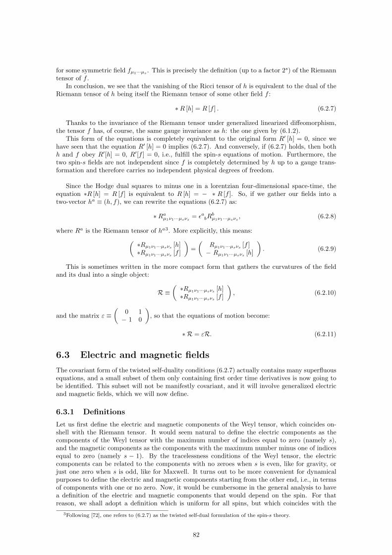
for some symmetric field fµ1···µs . This is precisely the definition (up to a factor 2s) of the Riemanntensor of f .

In conclusion, we see that the vanishing of the Ricci tensor of h is equivalent to the dual of theRiemann tensor of h being itself the Riemann tensor of some other field f :

∗R [h] = R [f ] . (6.2.7)

Thanks to the invariance of the Riemann tensor under generalized linearized diffeomorphism,the tensor f has, of course, the same gauge invariance as h: the one given by (6.1.2).

This form of the equations is completely equivalent to the original form R′ [h] = 0, since wehave seen that the equation R′ [h] = 0 implies (6.2.7). And conversely, if (6.2.7) holds, then bothh and f obey R′[h] = 0, R′[f ] = 0, i.e., fulfill the spin-s equations of motion. Furthermore, thetwo spin-s fields are not independent since f is completely determined by h up to a gauge trans-formation and therefore carries no independent physical degrees of freedom.

Since the Hodge dual squares to minus one in a lorentzian four-dimensional space-time, theequation ∗R [h] = R [f ] is equivalent to R [h] = − ∗ R [f ]. So, if we gather our fields into atwo-vector ha ≡ (h, f), we can rewrite the equations (6.2.7) as:

∗Raµ1ν1···µsνs = εabRbµ1ν1···µsνs , (6.2.8)

where Ra is the Riemann tensor of ha3. More explicitly, this means:(∗Rµ1ν1···µsνs [h]∗Rµ1ν1···µsνs [f ]

)=

(Rµ1ν1···µsνs [f ]− Rµ1ν1···µsνs [h]

). (6.2.9)

This is sometimes written in the more compact form that gathers the curvatures of the fieldand its dual into a single object:

R ≡(∗Rµ1ν1···µsνs [h]∗Rµ1ν1···µsνs [f ]

), (6.2.10)

and the matrix ε ≡(

0 1− 1 0

), so that the equations of motion become:

∗ R = εR. (6.2.11)

6.3 Electric and magnetic fields

The covariant form of the twisted self-duality conditions (6.2.7) actually contains many superfluousequations, and a small subset of them only containing first order time derivatives is now going tobe identified. This subset will not be manifestly covariant, and it will involve generalized electricand magnetic fields, which we will now define.

6.3.1 Definitions

Let us first define the electric and magnetic components of the Weyl tensor, which coincides on-shell with the Riemann tensor. It would seem natural to define the electric components as thecomponents of the Weyl tensor with the maximum number of indices equal to zero (namely s),and the magnetic components as the components with the maximum number minus one of indicesequal to zero (namely s − 1). By the tracelessness conditions of the Weyl tensor, the electriccomponents can be related to the components with no zeroes when s is even, like for gravity, orjust one zero when s is odd, like for Maxwell. It turns out to be more convenient for dynamicalpurposes to define the electric and magnetic components starting from the other end, i.e., in termsof components with one or no zero. Now, it would be cumbersome in the general analysis to havea definition of the electric and magnetic components that would depend on the spin. For thatreason, we shall adopt a definition which is uniform for all spins, but which coincides with the

3Following [72], one refers to (6.2.7) as the twisted self-dual formulation of the spin-s theory.

82

standard conventions given above only for even spins. It makes the Schwarzschild field “electric”,but the standard electric field of electromagnetism is viewed as “magnetic”. Since the electric(magnetic) components of the curvature of the spin-s field are the magnetic (electric) componentsof the curvature of the dual spin-s field, this is just a matter of convention, but this conventionmay be confusing when confronted with the standard Maxwell terminology.

Before providing definitions, we recall that the curvature Ri1j1···isjs of the three-dimensional“spin-s field” hi1···is given by the spatial components of the spacetime spin-s field hµ1···µs is com-pletely equivalent to its Einstein tensor (introduced in section 4.1.2) defined as:

Gi1···is =1

2sεi1j1k1 · · · εisjsksRj1k1···jsks . (6.3.1)

This tensor is completely symmetric and identically conserved,

∂i1Gi1i2···is = 0 (6.3.2)

In the sequel, when we shall refer to the Einstein tensor of the spin s field, we shall usually meanthis three-dimensional Einstein tensor (the four-dimensional Einstein tensor vanishes on-shell).

We now define precisely the electric and magnetic fields off-shell as follows:

• The electric field E i1···is of the spin-s field hµ1···µs is equal to the Einstein tensor Gi1···is ofits spatial components hi1···is ,

E i1···is = Gi1···is (6.3.3)

By construction, the electric field fully captures the spatial curvature and involves only thespatial components of the spin-s field. It is completely symmetric and conserved,

E i1···is = E(i1···is), ∂i1E i1i2···is = 0 (6.3.4)

• The magnetic field Bi1···is of the spin-s field hµ1···µsis equivalent to the components with

one zero of the space-time curvature tensor and is defined through

Bi1···is =1

2s−1R j2k2···jsks

0i1εi2j2k2 · · · εisjsks (6.3.5)

It contains one time (and s − 1 space) derivatives of the spatial components hi1···is , and sderivatives of the mixed components h0i2···is . The magnetic field is symmetric in its last s−1indices. It is also transverse on each index,

∂i1Bi1i2···is = 0, ∂i2Bi1i2···is = 0, (6.3.6)

and traceless on the first index and any other index,

δi1i2Bi1i2···is = 0. (6.3.7)

It is useful to make explicit the dependence of the magnetic field – or equivalently, R0i1j2k2···jsks– on h0i2···is . One finds

R0i1j2k2···jsks = ∂i1

(ds−1

(s−1)N)j2k2···jsks

+ “more” (6.3.8)

where “more” involves only spatial derivatives of hi1···is and where Ni1···is−1stands for

h0i1···is−1 , i.e., Ni1···is−1 ≡ h0i1···is−1 .

Similar definitions apply to the dual spin-s field fλ1···λs.

The electric and magnetic fields possess additional properties on-shell. First, the electric fieldis traceless as a result of the equation R′00i5···is −

12δ

00R′′i5···is = 0,

δi1i2E i1i2···is = 0. (6.3.9)

Second, the magnetic field is symmetric as a result of the equation R′0i4i5···is = 0,

Bi1···is = B(i1···is) = 0. (6.3.10)

We also note that there are no other independent components of the space-time curvature tensoron-shell, since components with more than one zero can be expressed in terms of components withone or no zero through the equations of motion.

83

6.3.2 Twisted self-duality in terms of electric and magnetic fields

It is clear that the twisted self-duality conditions (6.2.7) with all indices being taken to be spatialread (

E i1i2···is [h]E i1i2···is [f ]

)=

(Bi1i2···is [f ]−Bi1i2···is [h]

). (6.3.11)

It turns out that these equations are completely equivalent to the full set of twisted self-dualityconditions. This is not surprising since the components of the curvature tensor with two or morezeroes are not independent on-shell from the components with one or no zero. The fact that(6.3.11) completely captures all the equations of motion will be an automatic consequence of oursubsequent analysis and so we postpone its proof to later (Section 6.4.3 below, where the actionprinciple from which these equations derive is shown to be the same as the one obtained earlier byHamiltonian analysis).

6.3.3 Getting rid of the Lagrange multipliers

While a generic component of the curvature may contain up to s time derivatives, the twistedself-duality conditions (6.3.11) contain only the first-order time derivatives hi1···is and fi1···is . Onecan give the fields hi1···is and fi1···is as Cauchy data on the spacelike hypersurface x0 = 0. Thesubsequent values of these fields are determined by the twisted self-duality conditions up to gaugeambiguities. The Cauchy data hi1···is and fi1···is cannot be taken arbitrarily but must be such thattheir respective electric fields are both traceless since this follows from E = ±B and the fact thatthe magnetic field is traceless. The constraints are equivalent to the condition that the traces ofthe Einstein tensors of both h and f should be zero,

Gi1···is−2 [h] = 0, Gi1···is−2 [f ] = 0 (6.3.12)

The twisted self-duality conditions involve also the mixed components h0i2···is and f0i2···is .These are pure gauge variables, which act as Lagrange multipliers for constraints in the Hamiltonianformalism. It is useful for the subsequent discussion to get rid of them. Since they occur only inthe magnetic fields, and through a gradient, this can be achieved by simply taking a curl on thefirst index. Explicitly, from the twisted self-duality conditions (6.3.11) rewritten as

Ea i1···is = εab Bb i1···is (6.3.13)

(Ea i1···is ≡ E i1···is [ha], Ba i1···is ≡ Bi1···is [ha], a = 1, 2, (ha) = (h, f), εab = −εba, ε12 = 1), followsobviously the equation

εjki1∂kEa i1···is = εab εjki1∂

kBb i1···is (6.3.14)

which does not involve the mixed components h0i2···is or f0i2···is any more.The equations (6.3.14) are physically completely equivalent to (6.3.13). Indeed, it follows from

(6.3.14) thatEa i1···is = εab Bb i1···is (6.3.15)

where Bb i1···is differs from the true magnetic field Bb i1···is by an arbitrary gradient in i1, or, interms of the corresponding curvature components

Ra0i1j2k2···jsks = Ra0i1j2k2···jsks + ∂i1µaj2k2···jsks (6.3.16)

for some arbitrary µaj2k2···jsks with Young symmetry type

s− 1 boxes︷ ︸︸ ︷.

Now, the cyclic identity fulfilled by the curvature implies ∂[i1µaj2k2]···jsks = 0, i.e., in index-free

notation, d(s−1)µa = 0, and this yields µa = ds−1

(s−1)νa for some symmetric νaj2···js (see the Appendix

4.A). Comparing with (6.3.8), we see that this is just the ambiguity in Ra0i1j2k2···jsks due to thepresence of ha0j2···js . Therefore, one can absorb µaj2k2···jsks in a redefinition of the pure gaugevariables ha0j2···js and get thereby the equations (6.3.13).

It is in the form (6.3.14) that we shall derive the twisted self-duality conditions from a variationalprinciple.

84

6.4 Variational principle

6.4.1 Prepotentials

The searched-for variational principle involves as basic dynamical variables not the fields hai1···is ,which are constrained, but rather “prepotentials” that solve the constraints (6.3.12) and can bevaried freely in the action. The general solution of the constraint equation Ga i1···is−2 = 0 was, ofcourse, worked out in the previous chapter, since it is exactly the Hamiltonian constraint solvedin section 5.2.5: it implies the existence of prepotentials Zai1···is from which hai1···is derives, suchthat the Einstein tensor Ga i1···is of hai1···is is equal to the Cotton tensor Ba i1···is of Zai1···is .

The Cotton tensor Ba i1···is was defined by equation (4.2.15). It involves 2s − 1 derivatives ofthe prepotentials and possesses the property of being invariant under spin-s diffeomorphisms andWeyl symmetries,

δZai1···is = s∂(i1ρai2···is) +

s(s− 1)

2δ(i1i2σ

ai3···is). (6.4.1)

It is symmetric, transverse and traceless.Because of the gauge symmetries, the solution of the equation Ga i1···is [h] = Ba i1···is [Z] for

hai1···is involves ambiguities. To any given solution ha[Z] one can add an arbitrary variation ofhai1···is under spin-s diffeomorphisms. Furthermore Zai1···is and Zai1···is + δZai1···is (with δZai1···isgiven by (6.4.1)) yield ha[Z]’s that differ by a spin-s diffeomorphism.

The expression for the spin-s fields hai1···is in terms of the prepotentials Zai1···is was computedearlier. It is given in the Appendix 5.A for even spin and in the Appendix 5.B for odd spin.

6.4.2 Twisted self-duality and prepotentials

In terms of the prepotentials, the electric fields are given by:

Ea i1···is = Bai1···is [Z], (6.4.2)

while the magnetic fields have the property

ε i1kj ∂kBa ji2···is = Bai1···is [Z]. (6.4.3)

It follows that the twisted self-duality conditions (6.3.14) take the form

εi1jk∂jBa ki2···is [Z] = εabB

bi1···is [Z] (6.4.4)

in terms of the prepotentials: the curl of the Cotton tensor of one prepotential is equal to (±) thetime derivative of the other.

6.4.3 Action

In their form (6.4.4), the twisted self-duality conditions are easily checked to derive from thefollowing variational principle:

S[Z] =

∫d4x

[1

2εabZ

a i1···isBbi1···is − H

](6.4.5)

where the Hamiltonian is:

H = δab

[ s2 ]∑k=0

akG[k]a i1···is−2kG

[k]bi1···is−2k

. (6.4.6)

This is precisely the action obtained by the Hamiltonian analysis of Fronsdal covariant La-grangian action for the spin-s (see section 5.2.6). The coefficient ak have the same value as then,being uniquely determined (up to a global factor) by the gauge invariance of the prepotentials,(6.4.1). The kinetic term indeed produces the right-hand side of (6.4.4), and the global factor ofthe Hamiltonian can be checked by computing one term the left-hand side of (6.4.4) and comparingit with the corresponding term in the variation of the Hamiltonian.

85

Since we have started this chapter with Fronsdal description of higher spins and end up withthis action as an equivalent description of its field, we can conclude that the action proposed insection 5.2.6 was indeed the Hamiltonian action of the spin-s field.

We will examine again in Appendix 6.B exactly how the symmetries constraint this action. Inparticular, we will see that this action enjoys, in addition to the gauge invariance of its fields (theprepotentials), an invariance under rigid rotations in the plane of its two prepotentials, which isprecisel the off-shell form of electric-magnetic duality rotations, hereby generalized to all higherspin.

86

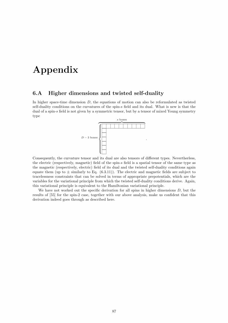
Appendix

6.A Higher dimensions and twisted self-duality

In higher space-time dimension D, the equations of motion can also be reformulated as twistedself-duality conditions on the curvatures of the spin-s field and its dual. What is new is that thedual of a spin-s field is not given by a symmetric tensor, but by a tensor of mixed Young symmetrytype

D − 3 boxes

s boxes︷ ︸︸ ︷.

Consequently, the curvature tensor and its dual are also tensors of different types. Nevertherless,the electric (respectively, magnetic) field of the spin-s field is a spatial tensor of the same type asthe magnetic (respectively, electric) field of its dual and the twisted self-duality conditions againequate them (up to ± similarly to Eq. (6.3.11)). The electric and magnetic fields are subject totracelessness constraints that can be solved in terms of appropriate prepotentials, which are thevariables for the variational principle from which the twisted self-duality conditions derive. Again,this variational principle is equivalent to the Hamiltonian variational principle.

We have not worked out the specific derivation for all spins in higher dimensions D, but theresults of [55] for the spin-2 case, together with our above analysis, make us confident that thisderivation indeed goes through as described here.

87

6.B Electric-magnetic duality

We saw earlier that the equations of motion of the spin one (section 3.1.1) and two (section 3.1.2)possess a duality invariance under SO(2) rotations in the plane of their (generalized) electric andmagnetic fields4. However, these rotations - called electric-magnetic duality transformations - arenot an apparent symmetry of their Lagrangian action - it is not even clear how to express theseduality transformations at the level of the field variables, Aµ or hµν . In order to make the off-shellform of these duality rotations explicit, it was necessary to go to the Hamiltonian formalism, wherethey appeared to be simply an SO(2) rotation in the plane of the two prepotentials (obtained bysolving the momentum and Hamiltonian constraints), under which the first order action was indeedinvariant.

The first order description developed in this chapter for all higher spin - which is equivalentto their Hamiltonian formalism, developed in the last chapter - precisely offers the possibility toextend these observations to all spin.

In D = 4 spacetime dimensions, the spin-s field hµ1···µs and its dual fµ1···µs are tensors ofthe same type, as we have seen (section 6.2). The equations enjoy then SO(2) electric-magneticduality invariance that rotates the field and its dual in the internal two-dimensional space thatthey span5. This comes over and above the twisted self-duality reformulation.

When one goes to the non-covariant formalism in which twisted self-duality conditions becomefirst order in time (section 6.3), the form (6.3.11) of the equations of motion obviously conservethis invariance under rotations in the h− f plane. Once the constraint part of these equations issolved and the prepotentials are introduced, it clearly appears that the SO(2) electric-magneticduality invariance amounts to perform rotations in the internal space of the prepotentials Zai1···is- since the prepotentials are such that their respective Cotton tensors are equal to the Einsteintensors of the spatial components of the h and f fields (or, equivalently, to the electric fields ofthe h and f fields). Again, the two prepotentials have the same type in D = 4: they are fullysymmetric (spatial) tensors.

We saw that the equations of motion in terms of the prepotentials (6.4.4) derived from theaction principle (6.4.5), which is also the Hamiltonian action of the spin-s. It is clear that thisaction is invariant under SO(2) rotations of the prepotentials Za.

Thus, the prepotential reformulation makes it obvious that SO(2) electric-magnetic dualityinvariance is a manifest off-shell symmetry, and not just a symmetry of the equations of motion.

6.B.1 How the symmetries fix the action

The Hamiltonian action principle of the spin-s in terms of its prepotentials - or the action fromwhich the first order in time twisted self-duality conditions can be extracted - is actually uniquelyfixed by its invariance under gauge transformations of the prepotentials (which combine spatialgeneralized linearized diffeomorphism with traceful parameters and generalized linearized Weylrescaling) and under electric-magnetic duality transformations, or SO(2) rotations in the plane ofthe two prepotentials6

This action is:

S[Z] =

∫d4x

[1

2εabB

a i1···isZbi1···is − H

](6.B.1)

where the Hamiltonian is:

H = δab

[ s2 ]∑k=0

akG[k]a i1···is−2kG

[k]bi1···is−2k

. (6.B.2)

The gauge invariance of the prepotentials is:

δZai1···is = s ∂(i1ρai2···is) +

s(s− 1)

2δ(i1i2σ

ai3···is). (6.B.3)

4This can also be described - and were introduced in section 3.1.1 and 3.1.2 - as rotation in the plane of thecurvature tensor and its Hodge dual.

5The equations of motion (6.2.9) are obviously invariant under rotations in the h− f plane.6These gauge and duality invariance only fix the action provided the quadratic presence of the prepotentials and

the number of spatial and time-like derivatives present are fixed. The global factors of the Hamiltonian and kineticterms remain, of course, undetermined.

88

The kinetic term in the action is manifestly invariant under the gauge symmetries of the prepo-tentials, because the Cotton tensor is both invariant under (6.B.3) and traceless. The Hamiltonianis manifestly invariant under the spin-s diffeomorphisms, since it involves the Einstein tensors ofthe prepotentials. It is also invariant under spin-s Weyl transformations up to a surface term, sinceits coefficients were precisely adjusted (and uniquely fixed, up to a global factor) in this purpose.

The action is furthermore manifestly invariant under SO(2) electric-magnetic duality rotationsin the internal plane of the prepotentials (we go back to the different naming of the two prepotentials(Zai1···is) ≡ (Pi1···is ,Φi1···is)):

Φ′i1···is = cos θΦi1···is − sin θPi1···is , (6.B.4)

P ′i1···is = cos θPi1···is + sin θΦi1···is , (6.B.5)

since it involves only the SO(2) invariant tensors εab and δab. As recalled in the introduction,exhibiting duality symmetry in the case of spin two was in fact the main motivation of [146] forsolving the constraints and introducing the prepotentials.

The gauge symmetries combined with duality invariance constrain the form of the action ina very powerful way. Indeed, the most general invariant quadratic kinetic term involving 2sderivatives of the prepotentials, among which one is a time derivative, is a multiple of the abovekinetic term. Similarly, the most general invariant quadratic Hamiltonian involving 2s spatialderivatives of the prepotentials is a mutiple of the above Hamiltonian7. By rescaling appropriatelythe time if necessary, one can therefore bring the action to the above form, which is consequently themost general gauge and duality invariant quadratic action with the required number of derivatives.

7SO(2) electric-magnetic duality invariance forces us to contract the prepotentials with SO(2) invariant tensors,either εab or δab, and it is easily seen that we need an antisymmetric tensor in the kinetic term and a symmetricone in the Hamiltonian, other choices leading to boundary terms.

89

Part III

Toward supersymmetry

90

Chapter 7

Hypergravity andelectric-magnetic duality

We have, up to this point, only considered free bosonic fields over flat space, whose dynamic andgeometry we have systematically studied: based on our investigation of higher spin three dimen-sional Euclidean conformal geometry (chapter 4), we have obtained the Hamiltonian formulation ofthese theories (chapter 5) and expressed their equations of motion as twisted self-duality conditions(chapter 6).

However, a large part of the physical interest of these bosonic theories comes from the possibilityof giving them a supersymmetric extension. We will not be able to explore thoroughly this vastand fascinating field in the present work, and we will limit ourselves to the opening of two pathwaysthat could lead to a better understanding of theories of significant interest.

In this chapter, we will begin to include fermions into the picture developed in the previous partin a very straightforward way, by considering the Hamiltonian analysis of a supermultiplet. Thesimplest supermultiplet including higher spin fields is the so-called hypergravity1, which pairs thegraviton with a spin-5/2 field2, as opposed to the well-known supergravity, in which the superpart-ner of the spin-2 is a spin-3/2 field. Hypergravity has been much less studied than supergravityfor the basic reason that the introduction of interactions seems impossible in the former, due towell-known no-go theorems 3.

Nevertheless, more recent investigations have led to the promising construction of possibleinteracting theories incorporating the spin-2 and 5/2 gauge fields, in addition to an infinite numberof other ones 4, so that the dynamic and symmetries of hypergravity might after all deserve someattention.

We will particularly be interested, here, into the way the electric-magnetic duality invariance ofthe spin two theory (reviewed in section 3.1.2) can be extended into a symmetry of hypergravitythat commutes with the supersymmetric (rigid) transformations that rotate the spin-2 and 5/2 fielsinto each other. Since we saw that electic-magnetic duality only becomes a manifest symmetryof the action in first order formalism, this suggests to make the Hamiltonian analysis of the spin-5/2 theory, which will show that the properties of the bosonic systems seem to still be present inthe fermionic ones: the solving of the Hamiltonian constraints leads to prepotentials whose gaugesymmetry includes both diffeomorphism and Weyl rescalings.

Remarkably, supersymmetry will map the two prepotentials of the graviton (the “momentum”and “field” prepotentials) into the single prepotential of the spin-5/2 in such a way that an electric-magnetic duality rotation of the graviton will be mapped by supersymmetry onto a chiral rotationof the fermion. In particular, this will allow us to combine an electric-magnetic duality transfor-mation of the boson with a chirality rotation of the fermion into a symmetry commuting withsupersymmetry. This generalizes similar results well-established for the “classic” supergravity5

1The “hyper” here refers to the fact that the fermionic superpartern has spin superior to the bosonic one. Thistermionology can be misleading, since hypersymmetry is a term often used to describe a symmetry whose parameteris a spinor-vector, as opposed to supersymmetry, for which it is a spinor.

2This theory has originally been studied in [6, 31,32].3See [6, 8]. Interactions can still be introduced in three spacetime dimensions, see [9]4This is the work of Lebedev school, see [111–113,215,218]. For a recent review: [27,92]5See [50].

91

We will begin by recalling the covariant formulation of hypergravity. We then turn in Section7.2 to the Hamiltonian formulation of the theory as this is necessary to manifestly exhibit duality.Section 7.3 provides the solution of the constraints of the Hamiltonian formulation in terms of theprepotentials. In Section 7.4, we write the supersymmetry transformations for the prepotentials. InSection 7.5, we give the expression of the action in terms of the prepotentials. The more technicalderivations are relegated to Appendix 7.A.

For comparison, we have also included an appendix 7.B which pursues the similar dualityanalysis for the spin-(1, 3/2) system.

7.1 Covariant form of hypergravity

7.1.1 Action

The action describing the combined system of a free spin-2 massless field, described by a symmetrictensor field hµν = hνµ, with a free spin-5/2 massless field, described by a symmetric spinor-rensorfield ψµν = ψνµ, is the sum of the actions of these two fields, introduced in equations (1.1.15) and(1.2.15) for an arbitrary spin:

S[hµν , ψµν ] =

∫d4x

(L2 + L 5

2

)(7.1.1)

where

L2 = − 1

2∂ρhµν∂ρhµν − 2 ∂ρhρµ∂νh

νµ + 2 ∂µhµν∂νh′ − ∂µh

′∂µh′ , (7.1.2)

and

L 52

= − i

ψµν /∂ψµν − 4 ψµργρ∂

νψµν + 2 ψµργρ /∂/ψµ + 2 ψµργρ∂µψ′ − 1

2ψ′ /∂ψ′

.

(7.1.3)

This fermionic action is not exactly the action introduced in (1.2.15), because we are now usinga spin-5/2 which is a “real” field (since we pair it with a real bosonic field into a supermultiplet):ψµν is taken to be a Majorana spinor-tensor. This allows us to rewrite a certain number of termsin (1.2.15) (through partial integrations), in order to get to (7.1.3).

7.1.2 Gauge symmetries

The action (7.1.1) is invariant under linearized diffeomorphisms

δgaugehµν = ∂µξν + ∂νξµ. (7.1.4)

and gauge transformations of the spin-5/2 field,

δgaugeψµν = ∂µζν + ∂νζµ, (7.1.5)

where the “spin-3/2” gauge parameter ζµ is γ-traceless,

/ζ = 0. (7.1.6)

Because of the tracelessness condition, one can express ζ0 in terms of ζk,

ζ0 = −γ0γkζk. (7.1.7)

There are three independent fermionic gauge symmetries.

92

7.1.3 Supersymmetry

The action is also invariant under rigid supersymmetry, which reads,

δSUSYhµν = 8i εψµν , (7.1.8)

δSUSYψµν = (∂µhνρ + ∂νhµρ) γρε − 2 ∂ρhµνγ

ρε

+(εµλσρ∂

λh σν + ενλσρ∂

λh σµ

)γργ5ε. (7.1.9)

The supersymmetry parameter ε is a constant spinor.

7.1.4 Equations of motion

The equations of motion can be written as

Rµν = 0 (7.1.10)

Fµν = 0 (7.1.11)

where Rµν is the linearized Ricci tensor of the spin-26 (see section 1.1.1) and Fµν the Fronsdaltensor of the spin-5/2 (see section 1.2.1). These tensors are given by:

Rµν = hµν − 2 ∂(µ∂ρhν)ρ + ∂µ∂νh

′, (7.1.12)

Fµν = /∂ψµν − 2 ∂(µ/ψν). (7.1.13)

The equations of motion and the action are invariant under electric-magnetic duality rotationsin the internal two-dimensional space spanned by the Riemann tensor Rµνρσ = 4 ∂[µ|∂[ρhσ]|ν] ofthe spin-2 and its dual (see section 3.1.2).

They are also invariant under chirality rotations of the spinor fields:

δchiralhµν = 0, δchiralψµν = λγ5ψµν (7.1.14)

That the action is invariant under chirality rotations is manifest. To display explicitly its electric-magnetic duality invariance, one must go to the first-order formalism and introduce prepotentialsfor the spin-two field. Supersymmetry forces one to then introduce prepotentials for the spin-five-half partner, as we now discuss. We will also see that a definite chirality rotation must accompanya duality transformation if duality is to commute with supersymmetry.

7.2 Hamiltonian form

7.2.1 Spin-2 part

As we recalled in section 2.2.2, the action of the graviton takes the canonical form:

S2 [Zakl] =1

2

∫d4x

εabZ

aklBbkl − δab

[GaklGbkl −

1

2GaGb

], (7.2.1)

where the prepotentials Zakl are related to the field hkl and its conjugate momenta Πkl (the variablesh0µ are Lagrange multipliers and do not have independent conjugate momenta; in this prepotentialformalism, they are absent) through:

Pkl = εkmpεlnq∂m∂nΦpq, (7.2.2)

hkl =1

2ε(k|mn∂

mφn|l) + 2 ∂(kξl), (7.2.3)

where the two prepotentials were renamed according to Zakl ≡ (Pkl, φkl).The gauge invariance of these prepotentials is given by:

δZakl = 2 ∂(kλl) + δklµa. (7.2.4)

The ξk are pure gauge.

6Note that Rµν is both the trace of the linearized Riemann tensor of the spin-2 and its Fronsdal tensor; seesection 1.1.1

93

7.2.2 Spin-5/2 part

We turn now to the spin-5/2 action. Its Hamiltonian formulation has been performed in [7, 37]but our treatment differs from these earlier works in that we do not fix the gauge at any stageand solve the (first-class) constraints through the introduction of prepotentials on which the fieldsdepend locally.

The action for the spin-five-half field, being already of first order, is almost in canonical form(see section 2.3.1 for the general formalism). Because there are gauge symmetries, some of thecomponents of ψµν are Lagrange multipliers for the corresponding first class constraints, whilethe other components define the phase space of the system. What differentiates the Lagrangemultipliers from the standard phase space variables is that the gauge variations of the formercontain the time derivatives ζm of the gauge parameters ζm, while the gauge variations of thelatter do not involve ζm.

To bring the action for the spin-five-half field to canonical form, we make the redefinition

Ξ = ψ00 − 2 γ0γkψ0k, (7.2.5)

ψ0k = ψ0k, (7.2.6)

ψmn = ψmn. (7.2.7)

One then has the following transformation rules,

δgaugeΞ = − 2 γkγl∂kζl (7.2.8)

δgaugeψ0k = ∂0ζk + γ0γl∂kζl (7.2.9)

δgaugeψkl = ∂kζl + ∂lζk, (7.2.10)

from which one immediately identifies the ψ0k components as the Lagrange multipliers. Indeed,the action takes the form:

S 52[Ξ, ψmn, ψ0k] =

∫d4x ΘA(ψB)ψA − H (ψB) + ψT0kFk (ψB), (7.2.11)

with (ψA) ≡ (Ξ, ψmn) and where the Hamiltonian H, the constraint functions Fk and the sym-plectic potential ΘA are explicitly given by,

H = − 3i

4Ξγk∂kΞ +

i

2ψklγm∂mψkl − 2i ψklγk∂

mψlm − i ψklγk∂lΞ

+ i ψklγk∂lψ +i

2Ξγk∂kψ −

i

4ψγl∂lψ + i ψklγ

lγmγn∂mψkn, (7.2.12)

Fk = i[∂kΞ − 2 ∂lψkl + ∂kψ + γkγ

l∂lΞ + 2 γlγm∂lψkm

− γkγl∂lψ + 2 γkγ

l∂mψlm], (7.2.13)

ΘΞ =i

4ΞT − i

2ψT , (7.2.14)

Θkl =i

2ψTkl −

i

4ψT δkl −

i

2ψTkmγ

mγl −i

2ψTlmγ

mγk. (7.2.15)

Here and from now on, ψ denotes the spatial trace ψ = ψkk. The action (7.2.11) is the searched-foraction in canonical form because the symplectic form ω = dΘ is non-degenerate and yields thefollowing brackets between the canonical variables,

Ξ (~x) ,Ξ (~x′)D = − 5i

4δ (~x− ~x′) , (7.2.16)

Ξ (~x) , ψkl (~x′)D =

i

4δkl δ (~x− ~x′) , (7.2.17)

ψkl (~x) , ψmn (~x′)D = δ (~x− ~x′)[− i

4(δkmδln + δknδlm) +

i

4δklδmn

+i

8(δkmγln + δknγlm + δlmγkn + δlnγkm)

].

(7.2.18)

94

These brackets would appear as Dirac brackets had one introduced conjugate momenta for thefermionic variables ψA and eliminated the corresponding second class constraints that expressthese momenta in terms of the ψA through the Dirac bracket procedure - hence the notation , D.The variables ψ0k are the Lagrange multipliers for the first-class constraints Fk = 0, which areeasily verified to generate the fermionic gauge transformations (7.2.8) and (7.2.10) through theDirac bracket.

7.3 Solving the constraints - Prepotentials

The fermionic constraint (7.2.13) can be rewritten in the simpler form

∂kΞ + ∂kψ + 2γij∂iψkj = 0 (7.3.1)

Indeed, if one multiplies (7.3.1) with k replaced by l by the invertible operator i(δlk + γkγ

l), one

gets Fk = 0. The equation (7.3.1) itself can be rewritten as ∂i(δikΞ + δikψ + 2γijψkj

)= 0, which

by virtue of the Poincare lemma implies

δikΞ + δikψ + 2γijψkj = ∂rA[ir]k (7.3.2)

for some tensor A[ir]k = −A[ri]

k, which can be decomposed into irreducible components as

A[ir]k = δika

r − δrkai + εirmmmk

with mmk = mkm. The equation (7.3.2) can be solved to yield ψij and Ξ in terms of ak and mij

as

2ψlk =1

2γlγm

(∂ka

m − 1

3δmk ∂qa

q + εqms∂qmsk

)−∂kal +

1

3δlk∂qa

q + ε qsl ∂qmsk (7.3.3)

Ξ = −2

3∂qa

q − ψ (7.3.4)

Now, the right-hand side of (7.3.3) is not symmetric in general, while ψlk is symmetric. The system

of equations (7.3.2) is overdetermined. A symmetric solution of (7.3.2) exists if and only if A[ir]k –

or equivalently, aq and mij – fulfills the constraints expressing that ψlk = ψkl. This condition is adifferential constraint which can be rewritten, by virtue of the Poincare lemma, as

akδql − alδ

qk +

1

2(γlγmδ

qk − γkγmδ

ql ) a

m − 1

3γlka

q

+ε qsl msk − ε qs

k msl +1

2γlγmε

qmsmsk −1

2γkγmε

qmsmsl

= ∂pBqplk (7.3.5)

for some tensor Bqplk antisymmetric in l, k and q, p, Bqplk = −Bqpkl = −Bpqlk . Trading each anti-symmetric pair for one single index using the Levi-Civita tensor, this tensor Bqplk is equivalent toa tensor Bij , B

lkqp ∼ εlkiεqpjBij , which can be decomposed into a symmetric part Σij and anantisymmetric part εijkV

k. The system (7.3.5) is a system of 9 linear spinorial equations for the9 spinorial unknows aq and mij = mji. We leave it to the reader to verify that this system can besolved uniquely for aq and mij in terms of the first derivatives of Σij and V k, which are thereforeunconstrained. Next, one substitutes the resulting expressions in (7.3.3) and (7.3.4), allowing in ad-dition for a general gauge transformation term in which one absorbs all gauge transformation termsinvolving Σij and V k through redefinitions. Then one finally gets the searched-for expressions

Ξ = 4Σ + ∂a∂bΣab − 2γkγl∂kvl (7.3.6)

ψij = δij4Σ− δij∂a∂bΣab − 24Σij −(γia∂

a∂bΣjb + γja∂a∂bΣib

)+(γia4Σaj + γja4Σai

)+ ∂ivj + ∂jvi (7.3.7)

95

of the fields Ξ and ψij in terms of a spin 5/2 prepotential Σij = Σji and a spin 3/2 prepotentialvi (in which V k has been completely absorbed). As a consistency check, it is easy to verifythat these expressions identically fulfill the spinorial constraint (7.3.1), as they should. Note thatthe prepotential vi drops out from gauge-invariant expressions and plays for that reason a lessfundamental role. It is similar to the prepotential ui for the graviton. One can easily verify thatthe expressions are invariant under the gauge symmetries of the prepotential Σij

δΣij = ∂iµj + ∂jµi + γiηj + γjηi (7.3.8)

where µi and ηi are arbitrary. Indeed, one finds δΞ = 0 and δψij = 0 provided one transformssimultaneously the other prepotential vi as

δvi = 24µi + γia∂a∂bµb − γia4µa − γa∂aηi + γi∂

aηa. (7.3.9)

Note that the special choice ηi = γiφ yields the Weyl rescaling 2φδij of the prepotential Σij , which istherefore contained among the gauge symmetries. The gauge transformations (7.3.8) are redundantsince one gets δΣij = 0 for µi = γiε and ηi = −∂iε. There are thus 3 × 4 (components of thevector-spinor µi) plus 3×4 (components of the vector-spinor ηi) minus 1×4 (reducibility relations)= 5 × 4 = 20 independant gauge parameters. The gauge transformations of the prepotentials viare mere shifts vi → vi + ωi where ωi are arbitrary vector-spinors. These prepotentials containtherefore no degree of freedon and can be set for instance equal to zero. The gauge transformations(7.3.8) are the only gauge symmetries of the prepotential Σij , as can be seen by mere counting.There are 6×4 = 24 components of the tensor-spinor Σij . These are unconstrained, but the gaugefreedom removes as we have just seen 20 components, leaving 4 independent arbitrary functionsneeded to describe the physical helicities of a massless spin-5/2 field. Another way to reach thesame conclusion goes as follows. One may rewrite (7.3.7) in terms of the Schouten tensor Sij [Σ]of Σij ,

Sij [Σ] =1

2(∂i∂

mΣmj + ∂j∂mΣmi −4Σij − ∂i∂jΣ)

−1

4(∂m∂nΣmn −4Σ) δij ,

asψij = 4Sij − 2γ ai Saj − 2γ aj Sai + ∂ivj + ∂j vi (7.3.10)

withvi = vi − 2∂mΣmi + ∂iΣ + γ ai ∂

bΣab − γ ai ∂aΣ (7.3.11)

which transforms asδvi = γk(∂iηk − ∂kηi) + 3γ km

i ∂mηk (7.3.12)

under (7.3.8). Similarly, one findsΞ = 4S − 2γkγl∂kvl. (7.3.13)

The Schouten tensor Sij [Σ] is invariant under linearized diffeomorphisms and “sees” only the γ-transformations. One finds explicitly

δSij [Σ] =

(−∂i∂j +

1

24)γkηk(

1

2(γi∂j + γj∂i)−

1

2δijγ

m∂m

)∂kηk

+1

2γk∂k (∂iηj + ∂jηi)

−1

2(γi4ηj + γj4ηi) (7.3.14)

under (7.3.8). Now, if ψij and Ξ are both equal to zero, one finds that the Schouten tensor is givenby

8Sij = −2∂mvmδij + ∂m(γ mj vi + γ m

i vj)

+∂i(γmj vm + vj) + ∂j(γ

mi vm + vi)

(7.3.15)

96

with vi constrained byγkγl∂kvl + ∂kvk = 0; (7.3.16)

By virtue of the Poincare lemma, the general solution of (7.3.16) is given by

vk = −7γm∂kηm + 8γk∂mηm − 9γm∂mηk + 5γ st

k ∂sηt (7.3.17)

for some arbitrary ηk. But then, (7.3.15) has exactly the form (7.3.14) of a γ-gauge transformation.This means that one can set the Schouten tensor Sij [Σ] – and hence also the Riemann tensor of Σijsince the number of dimensions is three – equal to zero by a γ-gauge transformation. This impliesthat in that γ-gauge, the tensor Σij itself is given by ∂iµj + ∂jµi, or, in general, by (7.3.8) if onedoes not impose any γ-gauge condition. This shows that (7.3.8) exhausts indeed the most generalgauge freedom. In parallel to what was found for the spin-2 prepotentials, the gauge symmetriesof the spin- 5

2 prepotential take the same form as the gauge symmetries of the free conformal spin5/2 field theory in 4 dimensions [110]. To make the comparison it should be borne in mind thatin [110], the redundancy in the gauge parameters is fixed by imposing the condition γiµi = 0. Ofcourse, two physically different theories may have the same gauge symmetries. It is neverthelessquite remarkable that gauge conformal invariance should emerge automatically when one requireselectric-magnetic duality invariance to be manifest. This is yet another evidence for the subtleinterplay between duality invariance and spacetime symmetry.

7.4 Supersymmetry transformations in terms of the prepo-tentials

A somewhat tedious but direct computation shows that the supersymmetry transformations of thebosonic prepotentials are given by

δΦij = −8iεχij (7.4.1)

andδPij = −8iεγ5χij . (7.4.2)

Here,

χij =1

2(εjmn∂

mΣ ni + εimn∂

mΣ nj

−εlmnγ lj ∂

mΣ ni − εlmnγ l

i ∂mΣ n

j ) (7.4.3)

transforms under gauge transformations of Σij in the same way as the bosonic prepotentials, i.e.,

δχij = ∂iαj + ∂iαj + δijβ,

for some αi and β. The details are given in Appendix 7.A. Similarly, one finds,

δΣij = 2γ5γ0(Φij − γ5Pij)ε, (7.4.4)

where again the gauge transformations match. Formulas (7.4.1), (7.4.2) and (7.4.4) are the analogsfor the spin-(2, 5/2) multiplet of the formulas (7.B.12), (7.B.14) and (7.B.16) giving the supersym-metry transformations of the prepotentials of the spin-(1, 3/2) multiplet. Even though the relation-ship between the original fields and the prepotentials is rather different for the two systems - theyinvolve only first-order derivatives for the lower spin multiplet, but also second-order derivativesfor the higher spin multiplet -, the final formulas giving the supersymmetry transformation rulesare remarkably similar and simple. In both cases, the transformation of the fermionic prepotentialinvolves the combination Mij ≡ Φij − γ5Pij (or Mi ≡ A2

i − γ5A1i ) of the two bosonic prepotentials

that transforms under duality asδdualMij = − α γ5Mij

(or δdualMi = − α γ5Mi). At the same time, the transformation of the first bosonic prepotentialΦij (or A1

i ) involves the function χij (or ψi) of the fermionic prepotential that has identical gaugetransformation properties as Φij (or A1

i ), while the transformation of the second prepotentialinvolves −γ5 times it.

97

7.5 Action

The action for the combined spin-(2, 5/2) system can be written in terms of the prepotentials. Onefinds by direct substitution,

S[Zaij ,Σij ] =

∫dt

[∫d3 x

(1

2εabBija Zbij + ΘAψA

)−H

], (7.5.1)

with

H =

∫d3x

[1

2

(GaklGbkl −

1

4GaGb

)δab +H

]. (7.5.2)

Here, B ija ≡ B ij [Za] (respectively G ij

a ≡ G ij [Za]) is the co-Cotton tensor (respectively, the Riccitensor) constructed out of the prepotential Zaij [53], whereas ΘA(Ξ(Σ), ψ(Σ)) and H(Ξ(Σ), ψ(Σ))are the functions of the second and third order derivatives of the prepotential Σij obtained bymerely substituting (7.3.6) and (7.3.7) in (7.2.14), (7.2.15) and (7.2.12). The action (7.5.1) ismanifestly separately invariant under duality rotations of the bosonic prepotentials Zaij :

δdualZ1ij = αZ2

ij , δdualZ2ij = −αZ1

ij (7.5.3)

and chirality rotations of the prepotential Σij ,

δchiralΣij = λγ5Σij , (7.5.4)

which implies δchiralψij = λγ5ψij . As such, neither the duality rotations (with untransformingfermions) nor the chirality transformations (with untransforming bosons) commute with super-symmetry. One can, however, extend the duality transformation to the fermionic prepotential insuch a way that duality and supersymmetry commute. This is done by combining the duality ro-tations of the bosonic superpotentials with a chirality transformation of the fermionic prepotentialof amplitude −α,

δdualΣjk = −α γ5Σjk. (7.5.5)

98

Appendix

7.A Technical derivations

7.A.1 Bosonic prepotential Zmn2 = φmn

The supersymmetry transformation rule of the graviton is

δhij = 8iεψij = 8iε[δij∆Σ− δij∂a∂bΣab

− 2∆Σij − γia∂a∂bΣjb − γja∂a∂bΣib+ γja∆Σai + γia∆Σaj + ∂iεj + ∂jεi

](7.A.1)

On the other handδhij = ∂rεirsδφ

sj + ∂rεjrsδφ

si + ∂iδvj + ∂jδvi. (7.A.2)

In order to compare these two expressions and find out the form of the supersymmetry transfor-mation of the graviton prepotential, δφij , it is useful to recast (7.A.1) in the form

δhij = −8iε[∂rεirsχ

sj + ∂rεjrsχ

si + ∂iηj + ∂jηi

](7.A.3)

This can be accomplished by setting

χjs =1

2

[εjmn∂

mΣns + εsmn∂mΣnj − εlmnγ l

j ∂mΣ n

s − εlmnγ ls ∂

mΣ nj

], (7.A.4)

and

εj = ηj −1

2∂jΣ +

3

2∂rΣjr +

1

2∂lγjlΣ +

1

2γal∂lΣja −

1

2∂rγjaΣra. (7.A.5)

Thus one concludes that, up to a gauge transformation,

δΦij = −8iεχij (7.A.6)

= −4iε(εjmn∂mΣ n

i + εimn∂mΣ n

j − εlmnγ lj ∂

mΣ ni − εlmnγ l

i ∂mΣ n

j ) (7.A.7)

and

δvi = −8iεηi (7.A.8)

= −8iε(εi +1

2∂iΣ−

3

2∂nΣin −

1

2∂rγirΣ +

1

2γis∂rΣ

sr − 1

2∂rγsrΣ

si ) (7.A.9)

Note that the field χij defined by (7.A.4) transforms as

δχij = ∂iαj + ∂jαi + δijβ (7.A.10)

with

αi =1

2

(εimn − εlmnγ l

i

)∂mµn + γ5ηi (7.A.11)

andβ = εlmnγ

l∂mηn (7.A.12)

under the gauge transformations (7.3.8) of the prepotential Σij .

99

7.A.2 Bosonic prepotential Zmn1 = Pmn

Using δhij = 8iεψij and the equation of motion of the hypergraviton

γρ∂ρψµν − ∂µγρψρν − ∂νγρψρµ = 0 (7.A.13)

one may write the supersymmetry transformation of the extrinsic curvature Kij = − 12 (∂0hij −

∂ih0j − ∂jh0i) asδKij = −2iεεmklγ5γkl [∂mψij − ∂iψmj − ∂jψmi] . (7.A.14)

Substituting the expression of ψij in terms of the fermionic prepotential Σij , one then finds

δKij = − 4iεγ0[δijγk∂

k (∆Σ − ∂m∂nΣmn) − 2 γk∂k∆ij

+ 2 γm∂i∂m∂nΣnj + 2 γm∂j∂

m∂nΣni + γkim∂k∆Σmj

+ γkjm∂k∆Σmi + γkjm∂

m∂n∂iΣnk + γkim∂

m∂n∂jΣnk]. (7.A.15)

As a corrolary, we get:

δK = − 4iεγ0[γk∂

k∆Σ + γm∂i∂m∂nΣni

]. (7.A.16)

and thus

δΠij = − δKij + δijδK

= 4iεγ0[− 2 δijγk∂

k∂m∂nΣmn − 2 γk∂k∆Σij + 2 γm∂i∂

m∂nΣnj

+ 2 γm∂j∂m∂nΣni − εikmγ

0γ5∂k∆Σmj − εjkmγ

0γ5∂k∆Σmi

+ εikmγ0γ5∂

k∂n∂jΣnm + εjkmγ

0γ5∂k∂n∂iΣ

nm]

(7.A.17)

Now, knowing the supersymmetry transformation δΦij = −8iεχij of the prepotential Φij andcomparing with the spin-1-spin-3/2 system, it is natural to guess that the supersymmetry trans-formation of the other bosonic prepotential Pij is simply

δPij = 8iεγ5χij (7.A.18)

To prove this claim, it suffices to compute δΠij from its definition in terms of Pij and (7.A.18),and verify that the resulting expression coincides with (7.A.17). The computation is direct. Onefinds

δΠij = − 8iεγ5 εiklεjmn∂k∂mχln

= − 4iεγ5

[εiklεjmnε

lrs∂k∂m∂rΣns + εiklεjmnε

nrs∂k∂m∂rΣls

− εiklεjmnεprsγnp∂k∂m∂rΣsl − εiklεjmnεprsγ

lp∂k∂m∂rΣsn]

= − 4iεγ5

[εjmn∂

k∂m∂iΣnk + εikl∂

k∂m∂jΣl

m − εjmn∂m∆Σ n

i − εikl∂k∆Σ l

j

− 2 δijεprsγnp∆∂rΣsn + 2 δijεprsγ

np∂n∂m∂rΣsm − εprsγ

np∂n∂i∂rΣsj

− εprsγjp∂n∂i∂rΣsn − εprsγip∂j∂

m∂rΣsm − εprsγmp∂j∂m∂

rΣsi

+ εprsγip∆∂rΣsj + εprsγjp∆∂rΣsi + εprsγnp∂j∂i∂

rΣsn

+ εprsγnp∂j∂i∂

rΣsn] . (7.A.19)

Using the identity γnp = γ0γ5εnpqγq, this expression becomes

δΠij = − 4iεγ0[− εjmnγ

0γ5∂k∂m∂iΣ

nk − εiklγ

0γ5∂k∂m∂jΣ

lm + εjmnγ

0γ5∂m∆Σ n

i

+ εiklγ0γ5∂

k∆Σ lj − 2 δijγr∂

r (∆Σ − ∂n∂mΣnm)

− 2 γr∂j∂m∂rΣim − 2 γr∂

n∂i∂rΣnj + 2 γr∆∂

rΣij + 2 γr∂j∂i∂rΣ] .(7.A.20)

The term 2γr∂j∂i∂rΣ− 2δijγr∂

r∆Σ is a gauge transformation of Πij , and can be removed, giving:

δΠij = − 4iεγ0[− εjmnγ

0γ5∂k∂m∂iΣ

nk − εiklγ

0γ5∂k∂m∂jΣ

lm + εjmnγ

0γ5∂m∆Σ n

i

+ εiklγ0γ5∂

k∆Σ lj + 2 δijγr∂

r∂n∂mΣnm + 2 γr∆∂rΣij

− 2 γr∂j∂m∂rΣim − 2 γr∂

n∂i∂rΣnj ] , (7.A.21)

which is exactly (7.A.17). This proves the correctness of (7.A.18).

100

7.A.3 Supersymmetric variation of the fermionic prepotential Σij

One can rewrite the supersymmetry transformation for ψµν as:

δψij = (∂ihjρ + ∂jhiρ)γρε− 2 ∂ρhijγ

ρε+ (εiλσρ∂λh σ

j + εjλσρ∂λh σ

i )γργ5ε

= δΠψij + δhψij , (7.A.22)

where:

δΠψij = (∂ihj0 + ∂jhi0)γ0ε− 2 ∂0hijγ0ε+ (εi0km∂

0h kj + εj0km∂

0h ki

−εi0km∂kh 0j − εj0km∂kh 0

i )γmγ5ε,

δhψij = (∂ihjk + ∂jhik)γkε − 2 ∂khijγkε+ (εikl0∂

kh lj + εjkl0∂

kh li )γ0γ5ε. (7.A.23)

We compute δΠψij and δhψij separately.

Term depending on the prepotential Z1mn = Pmn

Let us first focus on the term involving the extrinsic curvature. Adding to it the gauge transfor-mation δψij = (∂ihj0 + ∂jhi0)γ0ε− (εi0km∂jh

k0 + εj0km∂ihk0)γmγ5ε yields:

δΠψij = 2 (∂ihj0 + ∂jhi0 − ∂0hij)γ0ε+ (εi0km∂

0h kj − εi0km∂kh 0

j − εi0km∂jhk0

+εj0km∂0h ki − εj0km∂kh 0

i − εj0km∂ihk0)γmγ5ε

= 4 Kijγ0ε− 2 ε0ikmK

kj γ

mγ5ε− 2 ε0jkmKki γ

mγ5ε

= 4 (− Πij +Π

2δij)γ

0ε+ 2ε0ikmΠ kj γ

mγ5ε+ 2 ε0jkmΠ ki γ

mγ5ε. (7.A.24)

Using:

− 4 Πij + 2 Πδij = − 4 εiabεjcd∂a∂cP bd + 2 δijεmabε

mcd∂

a∂cP bd

= − 4 εiabεjcd∂a∂cP bd + εixyεjxyεmabε

mcd∂

a∂cP bd

= − 2 εiabεjcd∂a∂cP bd − εjmbεmcd∂i∂cP bd − εimbεmcd∂j∂cP bd

+εjmaεmcd∂

a∂cP di + εimaε

mcd∂

a∂cP dj , (7.A.25)

one finds:

δΠψij = −[2εiabεjcd∂

a∂cP bd − εjmaεmcd∂a∂cP di − εimaεmcd∂a∂cP d

j

]γ0ε

+2[ε0jnmεiabε

ncd∂

a∂cP bd + ε0inmεjabεncd∂

a∂cP bd]γmγ5ε

−εjmbεmcd∂i∂cP bdγ0ε− εimbεmcd∂j∂cP bdγ0ε, (7.A.26)

and by dropping again a gauge transformation for ψij the following supersymmetry transformationrule may be derived for χij :

δχ bj = 2∂mP

bj γ

mγ5ε− εjcd∂cP bdγ0ε− εbcd∂cPjdγ0ε. (7.A.27)

Term depending on the Z2mn = φmn prepotential

We turn now to δhψij . Expressing it in terms of the prepotential φmn gives:

δhψij = (∂ihjk + ∂jhik)γkε− 2 ∂khijγkε+ (εikl0∂

kh lj + εjkl0∂

kh li )γ0γ5ε

= ∂i(∂lεjlmφ

mk + ∂lεklmφ

mj)γ

kε+ ∂j(∂lεilmφ

mk + ∂lεklmφ

mi )γ

kε

−2 ∂k(∂lεilmφmj + ∂lφmi )γ

kε+ εikl0∂k(∂mεjmnφ

nl + ∂mεlmnφnj)γ

0γ5ε

+εjkl0∂k(∂mεimnφ

nl + ∂mεlmnφni)γ

0γ5ε

(7.A.28)

which, up to a gauge transformation, contributes to the supersymmetry transformation rule of χijas follows:

δχjm = −2∂kφjmγkε− (∂nεjnpφ

pm + ∂nεmnpφ

pj)γ

0γ5ε (7.A.29)

101

Finally, by adding up (7.A.27) and (7.A.29) the complete supersymmetry transformation rule forthe fermionic prepotential χij is obtained:

δχij = −2 ∂k(φij + Pijγ5)γkε+ εicd∂c(φdjγ5 − P d

j )γ0ε

+εjcd∂c(φdiγ5 − P d

i )γ0ε (7.A.30)

Using the identity εlxyγli = (δixγy−δiyγx)γ0γ5 in (7.A.4), one can see immediatly that this implies

the following transformation rule for the prepotential Σij ,

δΣij = 2 γ5γ0(φij − γ5Pij)ε (7.A.31)

102

7.B The spin-(1, 32) multiplet

7.B.1 Spin 1

The covariant action of the Maxwell field

S1[Aµ] = − 1

4

∫d4x FµνF

µν (7.B.1)

can be recast in a manifestly duality-invariant form by going to the first-order formalism andintroducing a second vector potential A2

i through the resolution of Gauss’ contraint [88] (see section2.2.1). One finds, in duality covariant notations:

I =1

2

∫dx0d3x

(εab ~B

a · ~Ab − δab ~Ba · ~Bb). (7.B.2)

Here, εab is given by εab = −εba, ε12 = +1 and

~Ba = ~∇× ~Aa,

with A1i ≡ Ai. The action (7.B.2) is invariant under rotations in the (1, 2) plane (“electric-magnetic

duality rotations”) , (~A1

~A2

)≡ ~A −→ eαε ~A (7.B.3)

because εab and δab are invariant tensors. In infinitesimal form,

δdualA1k = α A2

k, (7.B.4)

δdualA2k = − α A1

k. (7.B.5)

The action (7.B.2) is also invariant under U(1)× U(1) gauge transformations,

Aak −→ Aak + ∂kΛa.

7.B.2 Spin 3/2

The covariant action of the spin 3/2 is given by the expression (see section 1.2.1):

S3/2 = i

∫d4x ψµγ

µνρ∂νψρ (7.B.6)

which is invariant under the gauge transformation δψµ = ∂µε. This first-order action is already incanonical form, with ψk being self-conjugate canonical variables and ψ0 the Lagrange multiplierfor the constraint

0 = γkl∂kψl. (7.B.7)

The general solution of the constraint (7.B.7) (see section 2.3.2) reads [50]:

ψk = − 1

2εlmnγlγk∂mχn, (7.B.8)

where χk is a vector-spinor, which is the prepotential for the spin-3/2 field. The ambiguity in χkis given by [50],

δgaugeχk = ∂kη + γ0γ5γkε, (7.B.9)

where η and ε are arbitrary spinor fields. As observed in [50], these are the same gauge symmetriesas those of a conformal spin-3/2 field.

103

7.B.3 Supersymmetry

The supersymmetry transformations for the (1, 3/2)-multiplet read

δSUSYAµ = i εψµ, (7.B.10)

δSUSYψµ =1

4Fµνγ

νε +1

4Fµνγ5γ

νε. (7.B.11)

and are easily verified to leave the covariant action S1 + S3/2 invariant. The supersymmetrytransformations can be rewritten in terms of the prepotentials (Aak, χk). From the supersymmetrytransformation of the photon field (7.B.10), one immediately deduces that:

δSUSYA1k = i εψk, (7.B.12)

where ψk is now to be viewed as the function (7.B.8) of the prepotential χk. Similarly, a directcomputation shows that the supersymmetry transformation of the momentum Πk conjugate toAk ≡ A1

k ( minus the original electric field) is

δSUSYΠk = − i

2εklmεγ5∂lψm +

i

2εγ0γklm∂lψm

= − i εklmεγ5∂lψm. (7.B.13)

Since Πk = εklm∂lA2m, one gets

δSUSYA2k = − i εγ5ψk (7.B.14)

(up to a gauge transformation that can be set to zero). Finally, one easily derives from (7.B.11)

δSUSYψk = − 1

4Wkγ

0ε

+1

4εklmW

mγ5γlε. (7.B.15)

where we have defined Wk ≡ Πk − Bkγ5. It follows that, again up to a gauge transformation ofthe prepotential that can be set to zero,

δSUSYχk =

1

2

(A2k − A1

kγ5

)γ0ε

=1

2Mkγ

0ε (7.B.16)

withMk ≡ A2

k − A1kγ5 . (7.B.17)

The transformations (7.B.12), (7.B.14) and (7.B.16) are the searched-for supersymmetry transfor-mations in terms of the prepotentials. We close by noting that the duality rotations (7.B.4) and(7.B.5) with δχ = 0, and the chirality rotations

δchiralχk = λ γ5χk (7.B.18)

with δA1k = δA2

k = 0, separately leave the action invariant. None of these transformationscommutes with supersymmetry. However, the combined duality-chirality transformation (7.B.4),(7.B.5) and (7.B.18) with λ = −α commutes with supersymmetry. This is because Mk transformsas

δdualMk = − α γ5Mk (7.B.19)

under duality. In the case of extended supersymmetry, duality acting only on the vector fields willnot commute either with supersymmetry, but again it can be redefined to do so with one of thesupersymmetries.

104

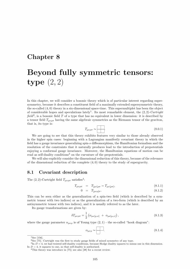
Chapter 8

Beyond fully symmetric tensors:type (2, 2)

In this chapter, we will consider a bosonic theory which is of particular interest regarding super-symmetry, because it describes a constituent field of a maximally extended supersymmetric theory,the so-called (4, 0) theory in a six-dimensional space-time. This supermultiplet has been the objectof considerable hopes and speculations lately1. Its most remarkable element, the (2, 2)-Curtrightfield2, is a bosonic field T of a type that has no equivalent in lower dimension: it is described bya tensor field Tµνρσ having the same algebraic symmetries as the Riemann tensor of the graviton,that is, its type is:

Tµνρσ ∼ . (8.0.1)

We are going to see that this theory exhibits features very similar to those already observedin the higher spin cases: beginning with a Lagrangian manifestly covariant theory in which thefield has a gauge invariance generalizing spin-s diffeomorphism, the Hamiltonian formalism and theresolution of the constraints that it naturally produces lead to the introduction of prepotentialsenjoying a conformal gauge invariance. Moreover, the Hamiltonian equations of motion can beread as self-duality conditions3 on the curvature of the prepotentials.

We will also explicitly consider the dimensional reduction of this theory, because of the relevanceof the dimensional reduction of the complete (4, 0) theory to the study of supergravity.

8.1 Covariant description

The (2, 2)-Curtright field Tµνρσ satisfies4:

Tµνρσ = T[µν]ρσ = Tµν[ρσ], (8.1.1)

0 = T[µνρ]σ. (8.1.2)

This can be seen either as the generalization of a spin-two field (which is described by a sym-metric tensor with two indices) or as the generalization of a two-form (which is described by anantisymmetric tensor with two indices), and it is usually referred to as the later.

Its gauge transformations are given by:

δTµνρσ =1

2

(αµν[ρ,σ] + αρσ[µ,ν]

), (8.1.3)

where the gauge parameter αµνρ is of Young type (2, 1) - the so-called “hook diagram”:

αµνρ ∼ . (8.1.4)

1See [156].2See [75]. Curtright was the first to study gauge fields of mixed symmetry of any type.3In D = 4, we had twisted self-duality conditions, because Hodge duality squares to minus one in this dimension.

In D = 4, it squares to one, so that self-duality is authorized.4This theory was introduce in [75]; see also [38] for a recent review.

105

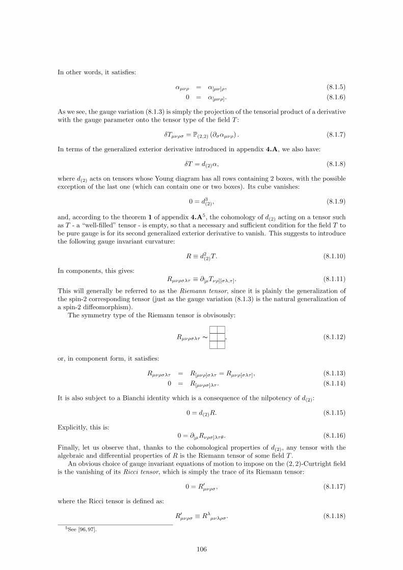
In other words, it satisfies:

αµνρ = α[µν]ρ, (8.1.5)

0 = α[µνρ]. (8.1.6)

As we see, the gauge variation (8.1.3) is simply the projection of the tensorial product of a derivativewith the gauge parameter onto the tensor type of the field T :

δTµνρσ = P(2,2) (∂σαµνρ) . (8.1.7)

In terms of the generalized exterior derivative introduced in appendix 4.A, we also have:

δT = d(2)α, (8.1.8)

where d(2) acts on tensors whose Young diagram has all rows containing 2 boxes, with the possibleexception of the last one (which can contain one or two boxes). Its cube vanishes:

0 = d3(2), (8.1.9)

and, according to the theorem 1 of appendix 4.A5, the cohomology of d(2) acting on a tensor suchas T - a “well-filled” tensor - is empty, so that a necessary and sufficient condition for the field T tobe pure gauge is for its second generalized exterior derivative to vanish. This suggests to introducethe following gauge invariant curvature:

R ≡ d2(2)T. (8.1.10)

In components, this gives:Rµνρσλτ ≡ ∂[µTνρ][σλ,τ ]. (8.1.11)

This will generally be referred to as the Riemann tensor, since it is plainly the generalization ofthe spin-2 corresponding tensor (just as the gauge variation (8.1.3) is the natural generalization ofa spin-2 diffeomorphism).

The symmetry type of the Riemann tensor is obvisously:

Rµνρσλτ ∼ , (8.1.12)

or, in component form, it satisfies:

Rµνρσλτ = R[µνρ]σλτ = Rµνρ[σλτ ], (8.1.13)

0 = R[µνρσ]λτ . (8.1.14)

It is also subject to a Bianchi identity which is a consequence of the nilpotency of d(2):

0 = d(2)R. (8.1.15)

Explicitly, this is:0 = ∂[µRνρσ]λτθ. (8.1.16)

Finally, let us observe that, thanks to the cohomological properties of d(2), any tensor with thealgebraic and differential properties of R is the Riemann tensor of some field T .

An obvious choice of gauge invariant equations of motion to impose on the (2, 2)-Curtright fieldis the vanishing of its Ricci tensor, which is simply the trace of its Riemann tensor:

0 = R′µνρσ, (8.1.17)

where the Ricci tensor is defined as:

R′µνρσ ≡ Rλµνλρσ. (8.1.18)

5See [96,97].

106

Its Young symmetry type is:

R′µνρσ ∼ . (8.1.19)

These equations of motion can actually be seen to derive from a variational principle, in whichthe gauge invariant Lagrangian is:

L = − 5

2δµ1...µ5ν1...ν5 M

ν1ν2ν3µ1µ2

M ν4ν5µ3µ4µ5

, (8.1.20)

where Mµνρστ = ∂[µTνρ]στ and δµ1...µ5ν1...ν5 = δµ1

[ν1· · · δµ5

ν5].

The construction outlined above offers additional possibilities of development in space-timedimension D = 2 + 2p (p even) where chiral p-forms exist. In our case, p = 2 and D = 6 is ofinterest, since our field generalizes a 2-form. Its Riemann tensor can naturally be subjected to aself-chirality condition, if one defines its dual as:

∗Rµνρσλτ ≡1

3!εµνραβγR

αβγσλτ . (8.1.21)

This dual tensor ∗R is not necessarily of the same symmetry type as R. However, a necessaryand sufficient condition for it to be so is for the trace of R to vanish, R′ = 0. In this case, ∗R,since it would also satisfy Bianchi identity, shall be the Riemann tensor of a field such as T . So,we can reformulate the equations of motion (8.1.19) as demanding that the dual of the Riemanntensor of T be itself the dual tensor of some field having the same algebraic symmetries and gaugeinvariance as T , which shall be the dual of T .

Since in D = 6 duality squares to one, (∗)2= 1, we can actually identify this dual field be

simply equal to T , and the equations of motion then take the elegant form of self-duality conditions:

R = ∗R. (8.1.22)

There is a mismatch between the number of equations (8.1.22), namely 175, and the num-ber of components of the (2, 2)-tensor field, namely 105. But the equations (8.1.22) are not allindependent.

We are now going to identify a complete subset of these equations which shall actually be offirst order in time derivative, but whose Lorentz invariance shall not be manifest. We will thensearch for a variational principle from which to extract them.

It is of course sufficient that the searched-for variational principle yields a system of equationsequivalent to (8.1.22).

8.2 Electric and magnetic fields

To identify such a subset derivable from a variational principle, we introduce the electric and mag-netic fields. The electric field contains the components of the curvature tensor with the maximumnumber of indices equal to the time direction 0, namely, two, E ijkl ∼ R0ij0kl, or what is the sameon-shell, the components of the curvature with no index equal to zero.

However, in 5 dimensions, the curvature tensor Rpijqkl is completely determined by the Einsteintensor, which is its spatial double Hodge dual:

Gijkl =1

(3!)2Rabcdefε ij

abc εdefkl (8.2.1)

= Rijkl − 2 δ[i[k

¯Rj]l] +

1

3δi[kδ

jl]

¯R, (8.2.2)

(the Weyl tensor identically vanishes).One then defines explicitly the electric field as:

E ijkl ≡ Gijkl. (8.2.3)

107

Here, Rijkl = Rmijmkl,¯Rjl = Rmijmil and

¯R = Rmijmij are the successive traces. Similar

conventions will be adopted below for the traces of the tensors that appear. The electric field hasthe (2, 2) Young symmetry and is identically transverse, ∂iE ijkl = 0. It is also traceless on-shell,

E ik ≡ E ijklδjl = 0. (8.2.4)

The magnetic field contains the components of the curvature tensor with only one index equalto 0,

Bijkl ≡1

3!R abc

0ij εabckl. (8.2.5)

It is identically traceless, Bjl ≡ Bijklδik = 0, and transverse on the second pair of indices,∂kBijkl = 0. On-shell, it has the (2, 2) Young symmetry.

The self-duality equation (8.1.22) implies:

E ijrs − Bijrs = 0. (8.2.6)

Conversely, the equation (8.2.6) implies all the components of the self-duality equation (8.1.22).This is verified in appendix 8.A by repeating the argument of [53] (recalled here in section 3.2.2)given there for a (2)-tensor, which is easily adapted to a (2, 2)-tensor. We have thus replaced theself-duality conditions (8.1.22) by a smaller, equivalent, subset. One central feature of this subsetis that it is expressed in terms of spatial objects.

Note that the trace condition (8.2.4) directly follows by taking the trace of (8.2.6) since themagnetic field is traceless. It appears as a constraint on the initial conditions because it does notinvolve the time derivatives of Tijrs. There is no analogous constraint in the p-form case.

Since the number of components of the electric field is equal to the number of spatial componentsTijrs of the (2, 2)-tensor Tαβλµ, one might wonder whether the equations (8.2.6) can be derivedfrom an action principle in which the basic variables would be the Tijrs. This does not work,however. Indeed, while the electric field involves only the spatial components Tijrs of the gaugefield, the magnetic field involves also the gauge component T0jrs, through an exterior derivative.One must therefore get rid of T0jrs.

To get equations that involve only the spatial components Tijrs, we proceed as in the 2-formcase and take the curl of (8.2.6), i.e.

εmnijk∂k(E rsij − B rs

ij

)= 0, (8.2.7)

eliminating thereby the gauge components T0jrs. We also retain the equation (8.2.4), which is aconsequence of (8.2.6) involving only the electric field. There is no loss of physical informationin going from (8.2.6) to the system (8.2.4), (8.2.7). Indeed, as shown in appendix 8.A, if (8.2.4)and (8.2.7) are fulfilled, one recovers (8.2.6) up to a term that can be absorbed in a redefinitionof T0jrs. The use of (8.2.4) is crucial in the argument. It is in the form (8.2.4), (8.2.7) that theself-duality equations can be derived from a variational principle.

8.3 Prepotentials - Action

To achieve the goal of constructing the action for the chiral tensor, we first solve the constraint(8.2.4) by introducing a prepotential Zijrs for Tijrs. Prepotentials were defined for gravity in [144](see section 2.2.2) and generalized to arbitrary symmetric tensor gauge fields in [132, 133] (seesection 5.2). The introduction of a prepotential for the mixed tensor Tijrs proceeds along similarlines.

Explicitly, the prepotential Zijrs provides a parametrization of the most general (2, 2) tensorfield Tijrs that solves the constraint (8.2.4). One has:

Tijrs = P(2,2)

(1

3!ε kmnij ∂kZmnrs

)+ gauge transf., (8.3.1)

which is a direct generalisation of the formula given in [146] for a (2)-tensor (see our equation(2.2.30)). The prepotential is determined up to the gauge symmetries:

δZijrs = P(2,2) (∂iξrsj + λirδjs) (8.3.2)

108

where ξrsj is a (2, 1)-tensor parametrizing the “linearized spin-(2, 2) diffeomorphisms” of the pre-potential and λir a symmetric tensor parametrizing its “linearized spin-(2, 2) Weyl rescalings”.

Because the Weyl tensor of a (2, 2)-tensor identically vanishes, the relevant tensor that controlsWeyl invariance is the “Cotton tensor”, defined as

Bijkl =1

3!εijabc∂

aSbckl , (8.3.3)

where:

Sijkl ≡ Gijkl − 2 δ

[i[kG

j]l] +

1

3δi[kδ

jl]

¯G (8.3.4)

is the “Schouten tensor”, which has the key property of transforming as:

δSijkl = − 4

27∂[j∂[kλ

i]l] (8.3.5)

under Weyl rescalings. In terms of our generalized exterior derivative (see appendix 4.A), thismeans:

δS = d(2)λ, (8.3.6)

where the tensors are of the symmetry type:

λ ∼ , S ∼ . (8.3.7)

The complete set of gauge invariants under (8.3.2) is, tanks to the cohomological properties of d(2),the tensor:

C ≡ d(2)S, (8.3.8)

or, in components:Cabckl ≡ ∂[aSbc]kl. (8.3.9)

Its symmetry type is:

C ∼ . (8.3.10)

Since we are in a five dimensional space, we can naturally dualize it over its first three indices,getting to the aforementioned Cotton tensor B. This is a straightforward generalization of whatwas done for completely symmetric tensors in section 4.2.

The Cotton tensor Bijkl is a (2, 2)-tensor which is gauge invariant under (8.3.2), as well asidentically transverse (this is a consequence of Bianchi identity d(2)C = 0) and traceless (this is aconsequence of the Young symmetry of C), ∂iB

ijrs = 0 = Bijrsδjs. Furthermore, a necessary andsufficient condition for Zijrs to be pure gauge is that its Cotton tensor vanishes.

The relation (8.3.1) implies that

E ijrs[T [Z]] ≡ Gijrs[T [Z]] = Bijrs[Z]. (8.3.11)

The relation (8.3.1) gives the most general solution for Tijrs subject to the constraint that E ijrsis traceless (this is proved in [132] - see our section 5.2.5 - for general higher spins described bycompletely symmetric tensors, and is easily extended to tensors with mixed Young symmetry). 6

It follows from (8.3.1) that

1

2εmnijk∂kB rs

ij = Bmnrs[Z] (8.3.12)

and therefore, in terms of the prepotential Zijrs, the self-duality condition (8.2.7) reads

1

2εmnijk∂kB

rsij [Z]− Bmnrs[Z] = 0, (8.3.13)

6We note that in three dimensions, the analogous relations on the Cotton tensor for symmetric gauge fields have anice supersymmetric interpretation [168,167,169]. It would be of interest to explore whether a similar interpretationholds here.

109

an equation that we can rewrite as

Lmnrs|ijpqZijpq = 0 (8.3.14)

where the differential operator Lmnrs|ijpq contains four derivatives and can easily be read off from(8.3.14). The operator Lmnrs|ijpq is symmetric, so that one can form the action

S[Z] =1

2

∫d6xZmnrs

(Lmnrs|ijpqZijpq

)(8.3.15)

=1

2

∫d6xZmnrs

(Bmnrs[Z]− 1

2εmnijk∂kB

rsij [Z]

)which yields (8.3.14) as equations of motion. Given that Z ∼ ∂−1T , this action contains the correctnumber of derivatives of T , namely two, and has therefore the correct dimension.

8.4 Chiral and non-chiral actions

The action (8.3.15) is our central result. Although not manifestly so, it is covariant. One way tosee this is to observe that (8.3.15) can be derived from the manifestly covariant (2, 2)-Curtrightaction for a (2, 2)-field [75, 38] rewritten in Hamiltonian form. As explained in appendix 8.B ,this action involves the spatial components Tijrs and their conjugate momenta πijrs as canonicallyconjugate dynamical variables, while the temporal components T0ijk and T0i0j play the role ofLagrange multipliers for the “momentum constraint”:

Cijk ≡ ∂lπijlk ≈ 0 (8.4.1)

and the “Hamiltonian constraint”:Cij ≡ E ikjk [T ] ≈ 0. (8.4.2)

These constraints can be solved by introducing two prepotentials Z(1)ijrs and Z

(2)ijrs. As for a

chiral 2-form [29], the linear change of variables:

(Z(1)ijrs, Z

(2)ijrs)→ (Z+

ijrs = Z(1)ijrs + Z

(2)ijrs, Z

−ijrs = Z

(1)ijrs − Z

(2)ijrs) (8.4.3)

splits the action as a sum of two independent terms, one for Z+ijrs and one for Z−ijrs. The Poincare

generators also split similarly, one for Z+ijrs and one for Z−ijrs, which transform separately. The

action (8.3.15) is the action for Z+ijrs obtained though this decomposition procedure, with the

identification Z+ijrs ≡ Zijrs. This second method for obtaining the action for a chiral (2, 2) tensor

shows as a bonus how a non-chiral (2, 2)-tensor dynamically splits as the sum of a chiral (2, 2)-tensorand an anti-chiral (2, 2)-tensor.

8.5 Dimensional reduction

Upon reduction from 5 + 1 to 4 + 1 dimensions, the prepotential Zijrs decomposes into a (2, 2)-tensor, a (2, 1)-tensor and a (2)-tensor. Using part of the Weyl symmetry, one can set the (2)-tensor equal to zero, leaving one with a (2, 2)-tensor and a (2, 1)-tensor which are exactly theprepotentials of the pure Pauli-Fierz theory in 4 + 1 dimensions [55], with the same action andgauge symmetries (see appendix 8.C). It is this remarkable connection between the (2, 2)-self-dualtheory in 6 spacetime dimensions and pure (linearized) gravity in 5 spacetime dimensions that isat the heart of the work [155,156]. We have shown here that the connection holds not just for theequations of motion, but also for the actions themselves.

8.6 Generalizations

The extension to more general two-column Young symmetry tensors is direct. The “critical dimen-sions” where one can impose self-duality conditions on the curvature are those where chiral p-forms

110

exist. The first colum of the Young tableau characterizing the Young symmetry must have p boxes,and the second column has then a number q ≤ p of boxes. So, in D = 6 spacetime dimensions,one has also the interesting case of (2, 1)-tensors, also considered in [155,156]. This case is treatedalong lines identical to those described here. For the next case – D = 10 spacetime dimensions–, the first column must have length 4, and the second colum has length q ≤ 4, an interestingexample being the (2, 2, 2, 2)-tensors. Again, the extension to this two-column symmetry case isdirect, as in all higher spacetime dimensions D = 14, 18, 22, 26, · · · .

The extension to more than two column Young symmetries is more subtle but proceeds asin [133], by relying on the crucial property demonstrated in [24], where it was shown that thesecond-order Fronsdal-Crurtright type equations can be replaced by equations on the curvatures,which involves higher order derivatives. The self-duality conditions can then be derived from anaction principle involving the appropriate prepotentials. The action is obtained by combining theabove derivation with the methods of [133] for introducing prepotentials.

The present analysis can be developed in various directions. First, following [155, 156], itwould be of great interest to consider the supersymmetric extensions of the 6-dimensional chiraltheory and to determine how the fermionic prepotentials enter the picture [50,56]. The attractive(4, 0)-theory of [155, 156] deserves a particular effort in this respect. Second, the inclusion ofsources, which would be dyonic by the self-duality condition, and the study of the correspondingquantization conditions, would also be worth understanding [82,202,51].

Finally, we note that we restricted the analysis to flat Minkowski space. The trivial topologyof Rn enabled us to integrate the differential equations for the prepotentials without encounteringobstructions, using the Poincare lemma of [96, 97]. The consideration of Minkowski space is notoptional at this stage since the coupling of a single higher spin field to curved backgrounds isproblematic. It is known how to surpass the problems only in the context of the Vasiliev theory,which requires an infinite number of fields [217,220,27,92,174]. Important ingredients to extend theanalysis of the present article to nonlinear backgrounds are expected to include the cohomologicalconsiderations of [29], the nonlinear extension of the higher spin Cotton tensors [170], as well asduality in cosmological backgrounds [165,164,152].

111

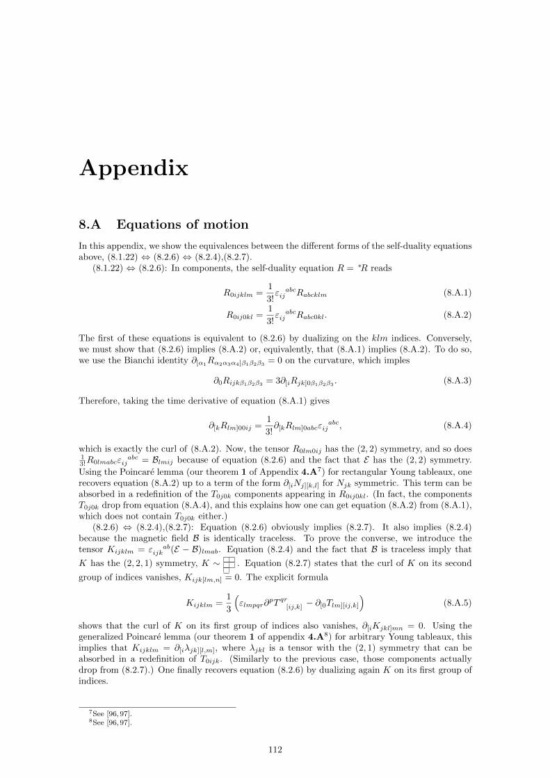
Appendix

8.A Equations of motion

In this appendix, we show the equivalences between the different forms of the self-duality equationsabove, (8.1.22) ⇔ (8.2.6) ⇔ (8.2.4),(8.2.7).

(8.1.22) ⇔ (8.2.6): In components, the self-duality equation R = ∗R reads

R0ijklm =1

3!ε abcij Rabcklm (8.A.1)

R0ij0kl =1

3!ε abcij Rabc0kl. (8.A.2)

The first of these equations is equivalent to (8.2.6) by dualizing on the klm indices. Conversely,we must show that (8.2.6) implies (8.A.2) or, equivalently, that (8.A.1) implies (8.A.2). To do so,we use the Bianchi identity ∂[α1

Rα2α3α4]β1β2β3= 0 on the curvature, which imples

∂0Rijkβ1β2β3= 3∂[iRjk]0β1β2β3

. (8.A.3)

Therefore, taking the time derivative of equation (8.A.1) gives

∂[kRlm]00ij =1

3!∂[kRlm]0abcε

abcij , (8.A.4)

which is exactly the curl of (8.A.2). Now, the tensor R0lm0ij has the (2, 2) symmetry, and so does13!R0lmabcε

abcij = Blmij because of equation (8.2.6) and the fact that E has the (2, 2) symmetry.

Using the Poincare lemma (our theorem 1 of Appendix 4.A7) for rectangular Young tableaux, onerecovers equation (8.A.2) up to a term of the form ∂[iNj][k,l] for Njk symmetric. This term can beabsorbed in a redefinition of the T0j0k components appearing in R0ij0kl. (In fact, the componentsT0j0k drop from equation (8.A.4), and this explains how one can get equation (8.A.2) from (8.A.1),which does not contain T0j0k either.)

(8.2.6) ⇔ (8.2.4),(8.2.7): Equation (8.2.6) obviously implies (8.2.7). It also implies (8.2.4)because the magnetic field B is identically traceless. To prove the converse, we introduce thetensor Kijklm = ε ab

ijk (E − B)lmab. Equation (8.2.4) and the fact that B is traceless imply that

K has the (2, 2, 1) symmetry, K ∼ . Equation (8.2.7) states that the curl of K on its second

group of indices vanishes, Kijk[lm,n] = 0. The explicit formula

Kijklm =1

3

(εlmpqr∂

pT qr[ij,k] − ∂[0Tlm][ij,k]

)(8.A.5)

shows that the curl of K on its first group of indices also vanishes, ∂[iKjkl]mn = 0. Using thegeneralized Poincare lemma (our theorem 1 of appendix 4.A8) for arbitrary Young tableaux, thisimplies that Kijklm = ∂[iλjk][l,m], where λjkl is a tensor with the (2, 1) symmetry that can beabsorbed in a redefinition of T0ijk. (Similarly to the previous case, those components actuallydrop from (8.2.7).) One finally recovers equation (8.2.6) by dualizing again K on its first group ofindices.

7See [96,97].8See [96,97].

112

8.B Hamiltonian formulation

The Lagrangian for a non-chiral (2, 2) tensor Tµνρσ is given by [38]

L = −5

2δµ1...µ5ν1...ν5 M

ν1ν2ν3µ1µ2

M ν4ν5µ3µ4µ5

, (8.B.1)

where Mµνρστ = ∂[µTνρ]στ and δµ1...µ5ν1...ν5 = δµ1

[ν1· · · δµ5

ν5]. The associated Hamiltonian action is

SH =

∫dt d5x

(πijklT

ijkl −H− nijk Cijk − nij Cij), (8.B.2)

where the Hamiltonian is

H = Hπ +HT (8.B.3)

Hπ = 3

(πijklπijkl − 2πijπij +

1

3π2

)(8.B.4)

HT =5

2δi1...i5j1...j5

M j1j2j3i1i2

M j4j5i3i4i5

. (8.B.5)

The components nijk = −4Tij0k and nij = 6T0i0j of T with some indices equal to zero only appearas Lagrange multipliers for the constraints

Cijk ≡ ∂lπijlk = 0 (8.B.6)

Cij ≡ E ikjk [T ] = 0. (8.B.7)

Those constraints are solved by introducing two prepotentials Z(1)ijkl and Z

(2)ijkl through

πijkl = Gijkl[Z(1)] (8.B.8)

Tijkl =1

3P(2,2)

(ε abcij ∂aZ

(2)bckl

). (8.B.9)

In terms of prepotentials, we have up to a total derivative

πijklTijkl = 2Z

(1)ijklD

ijkl[Z(2)] (8.B.10)

Hπ = 3Gijkl[Z(1)]Sijkl[Z(1)] (8.B.11)

HT = 3Gijkl[Z(2)]Sijkl[Z(2)]. (8.B.12)

Again up to a total derivative, one has Gijkl[Z]Sijkl[Z] = 13!Zijklε

ijabc∂aDkl

bc [Z]. Therefore,

defining the prepotentials Z±ijkl = Z(1)ijkl ± Z

(2)ijkl, the action splits into two parts, S[Z+, Z−] =

S+[Z+] − S−[Z−]. The action S+[Z+] is exactly the action (8.3.15) provided in the text fora chiral tensor, while S−[Z−] is the analog action for an anti-chiral tensor (which differs fromequation (8.3.15) only by the sign of the second term).

113

8.C Dimensional reduction

The prepotential decomposes into three tensors,

ZIJKL −→ Zijkl, Zijk5, Zi5j5. (8.C.1)

(For the purposes of this appendix, uppercase indices run from 1 to 5 while lowercase indices runfrom 1 to 4.) The (2, 2)-tensor and the (2, 1)-tensor are identified with the two prepotentials Pijkland Φijk for linearized gravity in 4 + 1 dimensions [55] as

Zijkl = 12√

3Pijkl, Zijk5 = −3√

3Φijk. (8.C.2)

The (2)-tensor Zi5j5 transforms under the Weyl symmetries (8.3.2) as δZi5j5 = 13 (λij +δijλ55) and

can therefore be set to zero. Remaining gauge transformations on Z must respect this choice: thisrestricts the gauge parameters to λij = −δijλ55 and ξi55 = 0. The surviving gauge parametersare then λ55, λi5, ξijk and ξ5ij . (Note that ξij5 = −2ξ5[ij] is not independent, due to the cyclicidentity ξ[IJK] = 0.) The map with the gauge parameters of [55] is

χijk = − ξijk

24√

3, Sij =

ξ5(ij)

12√

3, Aij = −

ξ5[ij]

12√

3

ξ =2λ55

9√

3, Bi =

2λi5

9√

3. (8.C.3)

This shows that field content and gauge symmetries match. For the comparison of the actions, oneneeds the following expressions for the reduction of the Cotton tensor:

D klij = − 2√

3εijab∂

a(Eklb + δb[kEl]) (8.C.4)

D k5ij = 2

√3 εijab∂

a(Rkb − 1

3δkbR) (8.C.5)

D j5i5 =

1√3εiabc∂

a(Ebcj + δjbEc), (8.C.6)

where Rij [P ] and Eijk[Φ] are defined as

Rij [P ] =1

(3!)2εiabcεjdef∂a∂fPbcde (8.C.7)

Eijk[Φ] =1

2.3!εijdeεkabc∂a∂eΦbcd (8.C.8)

and the traces are R = Rii, Ei = Eijj . Using these formulas, one recovers the action of [55] for

linearized gravity in 4 + 1 dimensions in the prepotential formalism.

114

Part IV

Surface charges on AdS

115

Chapter 9

Bose fields

9.1 Introduction

In theories with a gauge freedom, conserved quantities associated with the gauge symmetry aregiven by surface integrals (see section 2.4). We are now going to make a systematic investigation ofthese surface charges in the case of higher spin massless fields over AdS, through their Hamiltoniananalysis. Similarly to the flat space case considered above, this will lead us to first class constraintsgenerating gauge transformations.

These gauge transformations will have to be given a boundary term in order for their Poissonbracket with the fields to make sense. On-shell, the bulk part of these generators will identicallyvanish, since it is proportional to the constraints. On the other hand, the boundary term willprecisely give us the value of higher spin charges, provided the values plugged into the fields andgauge parameters appearing in it are carefully chosen. The fields will have to be given their on-shellvalue, so that their asymptotic behaviour will have to be evaluated through a (asymptotic) resolu-tion of Fronsdal equations of motion. As for the gauge parameters, they will have to correspond tovariations of the fields preserving their on-shell asymptotic behaviour while changing their physicalcontent.

This chapter is organised as follows: in order to highlight the key points of our analysis ofhigher-spin charges, we begin by discussing in section 9.2 the simplest example given by a spin-3field. We detail the Hamiltonian description of the free dynamics and we provide boundary con-ditions on the canonical variables that secure finiteness of charges. In section 5.2 we move toarbitrary spin: we first identify the Hamiltonian constraints that generate Fronsdal’s gauge trans-formations and then the associated charges. We eventually present boundary conditions inspiredby the behaviour at spatial infinity of the solutions of the free equations of motion (recalled inAppendix 9.C) and we verify that they give finite charges. We conclude summarising our resultsand discussing their expected regime of applicability. Other appendices provide a summary of ourconventions (Appendix 9.A) and more details on various results used in the main text (appendices9.B, 9.D and 9.E).

The next chapter is devoted to symmetric massless fermionic fields [65].

9.2 Spin-3 example

To compute surface charges within the canonical formalism, we first rewrite in Hamiltonian formthe Fronsdal action for a spin-3 field on an Anti de Sitter background of dimension d. The chargesare then identified with the boundary terms that enter the generator of gauge transformations andwe propose boundary conditions on fields and deformation parameters that secure their finiteness.The final expression for the charges is given in section 9.2.5, where we also compare our outcomewith other results in literature.

116

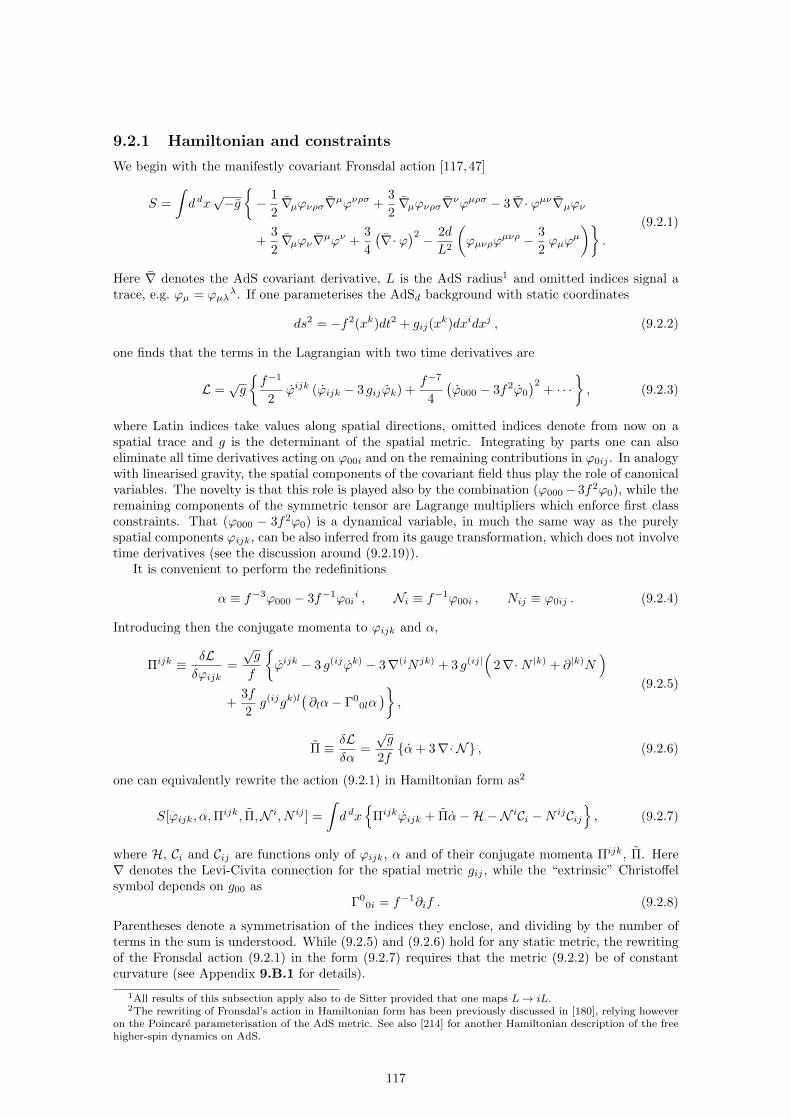
9.2.1 Hamiltonian and constraints

We begin with the manifestly covariant Fronsdal action [117,47]

S =

∫d dx√−g− 1

2∇µϕνρσ∇µϕνρσ +

3

2∇µϕνρσ∇νϕµρσ − 3 ∇· ϕµν∇µϕν

+3

2∇µϕν∇µϕν +

3

4

(∇· ϕ

)2 − 2d

L2

(ϕµνρϕ

µνρ − 3

2ϕµϕ

µ

).

(9.2.1)

Here ∇ denotes the AdS covariant derivative, L is the AdS radius1 and omitted indices signal atrace, e.g. ϕµ = ϕµλ

λ. If one parameterises the AdSd background with static coordinates

ds2 = −f2(xk)dt2 + gij(xk)dxidxj , (9.2.2)

one finds that the terms in the Lagrangian with two time derivatives are

L =√g

f−1

2ϕijk (ϕijk − 3 gijϕk) +

f−7

4

(ϕ000 − 3f2ϕ0

)2+ · · ·

, (9.2.3)

where Latin indices take values along spatial directions, omitted indices denote from now on aspatial trace and g is the determinant of the spatial metric. Integrating by parts one can alsoeliminate all time derivatives acting on ϕ00i and on the remaining contributions in ϕ0ij . In analogywith linearised gravity, the spatial components of the covariant field thus play the role of canonicalvariables. The novelty is that this role is played also by the combination (ϕ000− 3f2ϕ0), while theremaining components of the symmetric tensor are Lagrange multipliers which enforce first classconstraints. That (ϕ000 − 3f2ϕ0) is a dynamical variable, in much the same way as the purelyspatial components ϕijk, can be also inferred from its gauge transformation, which does not involvetime derivatives (see the discussion around (9.2.19)).

It is convenient to perform the redefinitions

α ≡ f−3ϕ000 − 3f−1ϕ0ii , Ni ≡ f−1ϕ00i , Nij ≡ ϕ0ij . (9.2.4)

Introducing then the conjugate momenta to ϕijk and α,

Πijk ≡ δLδϕijk

=

√g

f

ϕijk − 3 g(ijϕk) − 3∇(iN jk) + 3 g(ij|

(2∇·N |k) + ∂|k)N

)+

3f

2g(ijgk)l

(∂lα− Γ0

0lα)

,

(9.2.5)

Π ≡ δLδα

=

√g

2fα+ 3∇· N , (9.2.6)

one can equivalently rewrite the action (9.2.1) in Hamiltonian form as2

S[ϕijk, α,Πijk, Π,N i, N ij ] =

∫d dx

Πijkϕijk + Πα−H−N iCi −N ijCij

, (9.2.7)

where H, Ci and Cij are functions only of ϕijk, α and of their conjugate momenta Πijk, Π. Here∇ denotes the Levi-Civita connection for the spatial metric gij , while the “extrinsic” Christoffelsymbol depends on g00 as

Γ00i = f−1∂if . (9.2.8)

Parentheses denote a symmetrisation of the indices they enclose, and dividing by the number ofterms in the sum is understood. While (9.2.5) and (9.2.6) hold for any static metric, the rewritingof the Fronsdal action (9.2.1) in the form (9.2.7) requires that the metric (9.2.2) be of constantcurvature (see Appendix 9.B.1 for details).

1All results of this subsection apply also to de Sitter provided that one maps L→ iL.2The rewriting of Fronsdal’s action in Hamiltonian form has been previously discussed in [180], relying however

on the Poincare parameterisation of the AdS metric. See also [214] for another Hamiltonian description of the freehigher-spin dynamics on AdS.

117

The Hamiltonian in (9.2.7) reads explicitly

H = f

1√g

[1

2Πijk

(Πijk −

3

dgijΠk

)+ Π2

]+

3

2dΠi(∂iα− Γ0

0iα)

+√g

[1

2∇iϕjkl∇iϕjkl −

3

2∇iϕjkl∇jϕikl + 3∇· ϕij∇iϕj −

3

2∇iϕj∇iϕj −

3

4(∇· ϕ)

2

+2d

L2

(ϕijkϕ

ijk − 3

2ϕiϕ

i

)+ Γ0

0i

(3ϕijk∇jϕk −

3

2ϕi∇ · ϕ− 9

4Γ0

0jϕiϕj)

+5d− 3

8d∂iα∂

iα+d

L2α2 +

3(d+ 1)

8dgijΓ0

0i

(2α∂jα− Γ0

0jα2) ]

. (9.2.9)

The constraints are a generalisation of the Hamiltonian constraint in linearised gravity (but notehere the dependence on the additional momentum Π),

Ci = 3

∂iΠ−

√g

2

[2 (∆ϕi −∇· ∇· ϕi) +∇i∇· ϕ

− 4d− 1

L2ϕi − 3 Γ0

0j∇iϕj + 3 Γ00iΓ

00jϕ

j

],

(9.2.10)

and a generalisation of the constraint that generates spatial diffeomorphisms,

Cij = − 3

∇·Πij +

√g

2gij

(∆− d− 1

L2

)α

+√g

[Γ0

0(i∇j)α− Γ00iΓ

00jα+

1

2gijg

klΓ00k

(∂lα− Γ0

0lα)]

.

(9.2.11)

One can verify the absence of secondary constraints and that (9.2.10) and (9.2.11) are of first class.A simple way to convince oneself of these statements is to check that they provide the correctcounting of local degrees of freedom (see e.g. § 1.4.2 of [145]):

# d.o.f. =(d+ 1)!

3!(d− 2)!+ 1︸ ︷︷ ︸

canonical variables/2

−[

(d− 1)d

2+ (d− 1)

]︸ ︷︷ ︸

first-class constraints

=(d− 3)(d− 2)(d+ 2)

3!. (9.2.12)

The right-hand side is the dimension of a representation of so(d−2) labelled by a single-row Youngtableau with three boxes, as it is appropriate to describe a massless spin-3 particle in d space-timedimensions.

9.2.2 Gauge transformations

Being of first class, the constraints Ci = 0 and Cij = 0 generate gauge transformations. Thesecorrespond to the variation

δϕµνρ = 3 ∇(µΛνρ) (9.2.13)

that, in the covariant language, leaves the action (9.2.1) invariant provided that Λµν be traceless.In the canonical formalism, the generator of gauge transformations is

G[ξij , λi] =

∫d d−1x

(ξijCij + λiCi

)+Q1[ξij ] +Q2[λi] , (9.2.14)

where Q1 and Q2 are the boundary terms that one has to add in order that G[ξ, λ] admit welldefined functional derivatives, i.e. that its variation be again a bulk integral:

δG =

∫d d−1x

(AijkδΠ

ijk +Bijkδϕijk + CδΠ +Dδα). (9.2.15)

From (9.2.15) one can read the gauge transformations of the canonical variables as

δϕijk = ϕijk,G[ξ, λ] = Aijk , δΠijk = Πijk,G[ξ, λ] = −Bijk , (9.2.16a)

δα = α,G[ξ, λ] = C , δΠ = Π,G[ξ, λ] = −D . (9.2.16b)

118

The boundary terms Q1[ξ] and Q2[λ] give the asymptotic charges (see e.g. [195, 30]). Sensibleboundary conditions on the canonical variables must then be chosen such that the charges be finitewhen evaluated on deformation parameters which generate transformations preserving the givenboundary conditions.

Inserting the definitions (9.2.10) and (9.2.11) of the constraints in (9.2.14) and taking intoaccount that the background has constant curvature, one obtains

Aijk = 3∇(iξjk) , (9.2.17a)

Bijk = 3√g

∇(i∇jλk)− g(ij|

[(∆− 2(d− 1)

L2

)λ|k) +

1

2

(∇|k)+ 3 Γ0

0|k))∇· λ

], (9.2.17b)

C = − 3∇· λ , (9.2.17c)

D = − 3

2

√g

[(∆− 2d

L2

)ξ − Γ0

0i

(2∇· ξi + ∂iξ

)]. (9.2.17d)

The boundary terms generated by the integrations by parts putting the variation of G[ξ, λ] in theform (9.2.15) must be cancelled by the variations δQ1 and δQ2 of the charges. Being linear in thefields, these variations are integrable and yield:3

Q1[ξij ] = 3

∫d d−2Si

ξjkΠijk +

√g

2

[ξ∇iα− α∇iξ + Γ0

0j

(2 ξij + gijξ

)α]

, (9.2.18a)

Q2[λi] = 3

∫d d−2Si

− λiΠ +

√g

2

[2λj∇iϕj − 2λj∇· ϕij + λi∇· ϕ

− 2ϕj∇iλj + 2ϕijk∇jλk −∇· λϕi − 3 Γ00jλ

iϕj]

. (9.2.18b)

In presenting Q1 and Q2 we also adjusted the integration constants so that the charges vanish forthe zero solution.

Expanding (9.2.13) in components and comparing with (9.2.17a) and (9.2.17c), one can alsoidentify the deformation parameter ξij with the spatial components of the covariant gauge param-eter, while λi is related to Λµν by

λi = − 2f Λ0i . (9.2.19)

The remaining component of the covariant gauge parameter, Λ00, is proportional to gijξij thanks

to the Fronsdal constraint gµνΛµν = 0 that allows the cancellation of time derivatives in the gaugevariation of (ϕ000 − 3f2ϕ0). The other components of (9.2.13) give the gauge transformations ofthe Lagrange multipliers:

δNij = ξij + f(∇(iλj) − Γ0

0(iλj)), (9.2.20a)

δNi = λi + f(∂iξ − 2 Γ0

0iξ − 2 Γ00jξi

j). (9.2.20b)

Substituting the previous variations in the definitions of the momenta one can finally check theconsistency of (9.2.17b) and (9.2.17d) with Fronsdal’s gauge transformations. Notice that timederivatives only appear in the gauge transformations of Lagrange multipliers, in agreement withthe general results discussed e.g. in § 3.2.2 of [145]. This confirms once more our splitting of thecovariant field into canonical variables and Lagrange multipliers.

9.2.3 Boundary conditions

We now have to set boundary conditions on the canonical variables and restrict the deformationparameters to those that generate gauge transformations preserving them. Since we deal with thelinearised theory, we can actually fully specify the space of solutions of the equations of motion.

3Here dd−2Si ≡ dd−2x ni, where ni and dd−2x are respectively the normal and the product of differentials of thecoordinates on the d−2 sphere at infinity (e.g. d2x = dθdφ for d = 4, so that d2Si does not include the determinantof the intrinsic metric that appears in the full volume element).

119

We then extract boundary conditions from the behaviour at spatial infinity of the solutions in aconvenient gauge, with the expectation that the regime of applicability of both the charges (9.2.18)and the following fall-off conditions will extend even beyond the linearised regime (see section 9.4for an ampler discussion of this strategy).

In Appendix 9.C we recall the falloff at the boundary of the two branches of solutions of thesecond-order equations of motion imposed by the covariant action principle. In a coordinate systemin which the AdS metric reads

ds2 =dr2

r2+ r2 ηIJdx

IdxJ , (9.2.21)

the solutions in the subleading branch behave at spatial infinity (r →∞) as

ϕIJK = r3−d TIJK(xM ) +O(r1−d) , (9.2.22a)

ϕrIJ = O(r−d) , (9.2.22b)

ϕrrI = O(r−d−3) , (9.2.22c)

ϕrrr = O(r−d−6) . (9.2.22d)

We remark that capital Latin indices denote all directions which are transverse to the radial one(including time) and that here and in the following we set the AdS radius to L = 1. The fieldequations further impose that TIJK be conserved and traceless:

∂KTIJK = ηJKTIJK = 0 . (9.2.23)

We take (9.2.22) and (9.2.23) as the definition of our boundary conditions.In the case of spin 2 included in the discussion of section 9.3.2, for which the complete theory is

known in closed form (AdS gravity), the boundary conditions generally considered in the literatureagree with the behaviour of the solutions in the subleading branch [143, 46, 129]. Since in thiscase finiteness of the charges and consistency have been completely checked, we also adopt hereboundary conditions defined by the subleading branch, which is the direct generalisation of theseprevious works. It would be of interest to extend the analysis to more general asymptotics, as donefor scalar fields in [139,148,140], but we leave this question for future work. Furthermore, for d = 3the boundary conditions (9.2.22) agree with those in eq. (3.9) of [63], which have been derived fromthe Chern-Simons formulation of the full interacting theory of a spin-3 field with gravity.4

From (9.2.22) one directly gets the behaviour at spatial infinity of half of the canonical variables.Denoting the coordinates that parameterise the d− 2 sphere at infinity by Greek letters from thebeginning of the alphabet, one obtains

ϕαβγ = r3−d Tαβγ +O(r1−d) , α = − 2

rdT000 +O(r−d−2) , (9.2.24a)

ϕrαβ = O(r−d) , ϕrrα = O(r−d−3) , ϕrrr = O(r−d−6) . (9.2.24b)

To fix the behaviour of α we used the trace constraint on TIJK , which implies δαβT0αβ = T000.The boundary conditions on the momenta follow from the substitution of (9.2.24) in (9.2.5) and(9.2.6):

Πrαβ =d+ 1

r4T0αβ +O(r−6) , Π = O(r−4) , (9.2.25a)

Παβγ = O(r−7) , Πrrα = O(r−3) , Πrrr = O(1) . (9.2.25b)

In the formulae above we displayed explicitly only the terms which contribute to the charges (seesection 9.2.5). We expressed everything in terms of the components of the conserved boundarycurrent TIJK , but Tαβγ , T000 and T0

αβ can be considered only as convenient labels to denote the

4Actually in [63] the trace of ϕrIJ is even O(r−d−2) for the following reason: in the interacting theory – at leastin d = 3 – the fall-off conditions (9.2.22) are not preserved by asymptotic symmetries unless the fields also satisfythe equations of motion up to an order in r which depends on the highest spin appearing in the model. As we shallsee, these additional specifications are anyway irrelevant to compute charges.

120

boundary values of, respectively, ϕαβγ , α and Πrαβ . The covariant boundary conditions (9.2.22)would also fix the falloff of the Lagrange multipliers. The resulting conditions, however, wouldcorrespond to a particular choice of gauge, while – as noticed in three space-time dimensions[141, 57] – the freedom in the choice of the Lagrange multipliers is instrumental in fitting somephysically relevant solutions within the boundary conditions (see also [14]). We postpone to futurework a detailed analysis of this issue, especially because this freedom does not affect charges.

9.2.4 Asymptotic symmetries

As a next step we identify asymptotic symmetries, that are the gauge transformations preservingboundary conditions. Our goal is to specify appropriate deformation parameters in the generatorof gauge transformations (9.2.14). We begin however by selecting covariant gauge transformationscompatible with the fall-off conditions (9.2.22), to later identify the corresponding deformationparameters using e.g. (9.2.19).

Asymptotic symmetries contain at least the “higher-rank isometries” of the AdS space, i.e. thegauge transformations leaving the vacuum solution gµν = gAdS

µν and ϕµνρ = 0 invariant. These aregenerated by traceless AdS Killing tensors, satisfying

∇(µΛνρ) = 0 , gµνΛµν = 0 , (9.2.26)

where the latter condition is the usual Fronsdal constraint. These equations have been studied

e.g. in [211, 26, 15]: they admit (d−2)(d+1)(d+2)(d+3)12 independent solutions, obtained as traceless

combinations of symmetrised products of AdS Killing vectors [211]. This guarantees that non-trivial asymptotic symmetries do exist. We shall also notice that – as far as the free theory ind > 3 is concerned – asymptotic and exact Killing tensors only differ in terms that do not contributeto surface charges. It is nevertheless instructive to specify asymptotic Killing tensors in a unifiedframework that applies for any d ≥ 3.

In Appendix 9.C.2 we recall the behaviour at the spatial boundary of traceless AdS Killingtensors in the coordinates (9.2.21). We assume that asymptotic Killing tensors have the sameleading behaviour at r →∞, that is

ΛIJ = χIJ(xK) +

∞∑n= 1

r−2n χIJ(n)(xK) , (9.2.27a)

ΛrI = r wI(xK) +

∞∑n= 1

r1−2n wI(n)(xK) , (9.2.27b)

Λrr = r2 u(xK) +

∞∑n= 1

r2−2n u(n)(xK) , (9.2.27c)

and we now analyse the constraints imposed by the preservation of boundary conditions. Noticethat Λrr and the trace of ΛIJ are not independent: Fronsdal’s constraint gives

Λrr = −r4 ηIJΛIJ . (9.2.28)

As a result χIJ in (9.2.27a) is traceless, while the trace of χIJ(n+1) is proportional to u(n).

For any value of the space-time dimension d, the variation δϕIJK induced by (9.2.27) decaysslower at spatial infinity than the boundary conditions (9.2.22):

δϕIJK = 3 r4∂(IχJK) + 2 η(IJwK)

+O(r2) . (9.2.29)

The expression between parentheses must therefore vanish; this requires that χIJ be a tracelessconformal Killing tensor for the Minkowski metric ηIJ (see e.g. [99]),5

∂(IχJK) −2

d+ 1η(IJ ∂ · χK) = 0 , ηIJχ

IJ = 0 , (9.2.30)

5For simplicity we fixed the coordinates (9.2.21) such that the boundary metric is the flat Minkowski metric, but(9.2.30) is invariant under conformal rescalings of the boundary metric. See e.g. [63] for a discussion of this issue inthe d = 3 example, that can be extended verbatim to d > 3.

121

and that wI be fixed as

wI = − 1

d+ 1∂ · χI . (9.2.31)

As recalled in Appendix 9.D, when d > 3 the equations (9.2.30) – here defined in d− 1 dimensions –admit the same number of independent solutions as the equations (9.2.26). It is therefore notsurprising that their solutions can be extended to solutions of the Killing equation (9.2.26), providedone fixes the subleading components of the gauge parameter in terms of χIJ . As a result, in thelinearised theory asymptotic Killing tensors coincide with traceless Killing tensors of the AdS spaceup to a certain order in r, except in d = 3 where the equations (9.2.30) admit locally infinitelymany solutions.

To prove the previous statement, let us look at the variations of the other components with atleast one transverse index:

δϕrIJ =

∞∑n= 1

r3−2n−2nχ

(n)IJ − 2 ηIJχ

(n) + 2 ∂(Iw(n−1)J)

, (9.2.32a)

δϕrrI =

∞∑n= 1

r−2n−4nw

(n)I − ∂Iχ(n)

. (9.2.32b)

The leading order must cancel for any d and this requires

χ(1)IJ = − 1

d+ 1

(∂(I∂ · χJ) −

1

dηIJ∂ · ∂ · χ

), w

(1)I =

1

4d(d+ 1)∂I∂ · ∂ · χ . (9.2.33)

Substituting in δϕIJk one discovers that the first subleading order in (9.2.29) vanishes as wellprovided that

∂(I∂J∂ · χK) −3

2dη(IJ∂K)∂ · ∂ · χ = 0 . (9.2.34)

This identity is shown to follow from (9.2.30) in Appendix 9.D.The subleading orders can be analysed in a similar way. From (9.2.32) one sees that the

boundary conditions (9.2.22b) and (9.2.22c) are preserved provided that for 1 < n < d+12 one has

χ(n)IJ =

(−1)n(d− 1)!

4n−1n!(d+ n− 2)!(d+ 1)

(∂I∂J −

1

d+ n− 1ηIJ

)n−2∂ · ∂ · χ, (9.2.35a)

w(n)I =

(−1)n+1(d− 1)!

4nn!(d+ n− 1)!(d+ 1)n−1∂I∂ · ∂ · χ . (9.2.35b)

Computing three divergences of the conformal Killing equation (9.2.30) one finds however

(d− 1) ∂ · ∂ · χ = 0 , (9.2.36)

so that all w(n)I with n > 1 and all χ

(n)IJ with n > 2 vanish when d > 1. This also implies u(n) = 0

for n ≥ 1 thanks to the trace constraint (9.2.28) and, in its turn, that the condition (9.2.22d) is

preserved (χ(2)IJ does not vanish but it is traceless).

The variation of the transverse component thus reduces to

δϕIJK =1

8d(d+ 1)∂I∂J∂K∂ · ∂ · χ+O(r3−d) . (9.2.37)

The term written explicitly must vanish in all space-time dimensions except d = 3 and, indeed, inAppendix 9.D we prove that (9.2.30) implies

(d− 3) ∂I∂J∂K∂ · ∂ · χ = 0 . (9.2.38)

In d = 3 this identity is not available and one has two options: if one wants to solve the Killingequation (9.2.26) one has to impose the cancellation of the triple gradient of ∂ · ∂ ·χ and the addi-tional condition is satisfied only on a finite dimensional subspace of the solutions of the conformalKilling equation (9.2.30). If one is instead interested only in preserving the boundary conditions(9.2.22), which is the only option when the background is not exact AdS space, a shift of ϕIJK at

122

O(1) is allowed. The corresponding variation of the surface charges is at the origin of the centralcharge that appears in the algebra of asymptotic symmetries (see sect. 3.4 of [63]).

To summarise: parameterising the AdSd background as in (9.2.21), linearised6 covariant gaugetransformations preserving the boundary conditions (9.2.22) are generated by

ΛIJ = χIJ − r−2

d+ 1

(∂(I∂ · χJ) − 1

dηIJ∂ · ∂ · χ

)+

r−4

8d(d+ 1)∂I∂J∂ · ∂ · χ (9.2.39a)

+O(r−d−3) ,

ΛrI = − r

d+ 1∂ · χI +

r−1

4d(d+ 1)∂I∂ · ∂ · χ+O(r−d−2) , (9.2.39b)

Λrr =r2

d(d+ 1)∂ · ∂ · χ+O(r−d−1) , (9.2.39c)

where χIJ satisfies the conformal Killing equation (9.2.30), whose general solution is recalled in(9.D.3). In section 9.2.2 we have seen that the deformation parameter ξij has to be identified withthe spatial components of the covariant gauge parameter Λµν , while the deformation parameter λi

is related to Λµν by (9.2.19). Combining this information with (9.2.39), one sees that asymptoticsymmetries are generated by deformation parameters behaving as

ξαβ = χαβ +O(r−2) , λα = − 2r χ0α +O(r−1) , (9.2.40a)

ξrα = O(r) , ξrr = O(r2) , λr = O(r2) . (9.2.40b)

As in (9.2.24), Greek letters from the beginning of the alphabet denote coordinates on the d − 2sphere at infinity and we specified the dependence on χIJ only in the terms that contribute tosurface charges. In particular, as for gravity, when d > 3 the charges are insensitive to thedifferences between asymptotic and exact Killing tensors, corresponding the unspecified subleadingorders in (9.2.39).

9.2.5 Charges

Having proposed boundary conditions on both canonical variables (see (9.2.24) and (9.2.25)) anddeformation parameters (see (9.2.40)), we can finally evaluate the asymptotic charges (9.2.18). Inthe coordinates (9.2.21), the normal to the d− 2 sphere at infinity is such that nr = 1 and nα = 0.At the boundary the charges thus simplify as

limr→∞

Q1[ξij ] = 3

∫d d−2x

ξαβΠrαβ+

√g

2grrgαβ

(ξαβ∂rα− α∇rξαβ + Γ0

0rξαβα

), (9.2.41a)

limr→∞

Q2[λi] = 3

∫d d−2x

√g grrgαβ

λγ∇rϕαβγ + λγΓδrαϕβγδ − ϕαβγ∇rλγ

. (9.2.41b)

The terms which survive in the limit give a finite contribution to the charges; one can make thismanifest by substituting their boundary values so as to obtain

limr→∞

Q1 = 3(d+ 1)

∫d d−2x

(χαβT0αβ + χ00T000

), (9.2.42a)

limr→∞

Q2 = 6(d+ 1)

∫d d−2xχ0αT00α , (9.2.42b)

where we used the trace constraints on both χIJ and TIJK . When one sums both charges, theresult partly covariantises in the indices transverse to the radial direction:

Q ≡ limr→∞

(Q1 +Q2) = 3(d+ 1)

∫d d−2xχIJT0IJ . (9.2.43)

6A similar analysis has been performed in d = 3 including interactions [63]. These introduce a dependence onthe boundary values of the fields in (9.2.39), while asymptotic Killing tensors are still in one-to-one correspondencewith the solutions of the conformal Killing equation.

123

The boundary charge thus obtained is manifestly conserved: it is the spatial integral of the timecomponent of a conserved current since

JI ≡ χJKTIJK ⇒ ∂ · J = ∂(IχJK)TIJK + χJK∂ · TJK = 0 , (9.2.44)

where the conservation holds thanks to (9.2.23) and (9.2.30). We recovered in this way the standardpresentation of the global charges of the boundary theories entering the higher-spin realisations ofthe AdS/CFT correspondence (see e.g. sect. 2 of [123] for a review).

In three space-time dimensions, the rewriting (9.2.43) exhibits the chiral splitting of chargesthat one obtains in the Chern-Simons formulation with a suitable choice of the boundary valueof the Lagrange multipliers [142, 60, 57]. Introducing the light-cone coordinates x± = t ± φ, oneobtains

Qd=3 = 12

∫dφ(χIJT+IJ + χIJT−IJ

)= 12

∫dφ(χ++T+++ + χ−−T−−−

)= 12

∫dφ(χ(x+)T (x+) + χ(x−)T (x−)

),

(9.2.45)

where we took advantage of the form of the general solutions of (9.2.23) and (9.2.30), see e.g. (9.D.4).The separation in Q1 and Q2 does not correspond, however, to the splitting in left and right-movingcomponents since

limr→∞

Q1 = 6

∫dφ (χ+ χ)(T + T ) , lim

r→∞Q2 = 6

∫dφ (χ− χ)(T − T ) . (9.2.46)

The analysis of the linearised theory allowed us to recover the expression (9.2.45) that alsoholds in the non-linear theory [142,60], in line with our general expectations. Note, however, thatin d > 3 the asymptotic symmetries (9.2.39) leave the charges (9.2.43) invariant, while in d = 3only a variation of (9.2.45) which is independent of T and T is allowed. Since the variation of thecharges is generated by the charges themselves [45] as

δξ2Q[ξ1] = Q[ξ1], Q[ξ2] , (9.2.47)

one concludes that – although the linearised theory suffices to identify the charges – their algebradoes depend on interactions. As discussed in section 9.4, this phenomenon is anyway not apeculiarity of higher-spin theories. For an explicit example of the correlation between algebras ofcharges and interactions we refer to [63] where, assuming the expression (9.2.45) for spin-3 chargesin d = 3, their algebra has been computed by including the first interaction vertices in a weak-fieldexpansion in the spin-3 field.

We conclude this section by explicitly comparing our results with the higher-spin charges derivedfrom Fronsdal’s action in [15] within the covariant approach of [16,18].7 In the latter context, thespin-3 charges are given by the integral on a closed d−2 surface of the on-shell closed (d−2)-form

k[Λ] =1

2(d− 2)!k[µν][Λ] εµνρ3···ρddx

ρ3 · · · dxρd , (9.2.48)

with

k[µν][Λ] =√−gϕρσ

[µ∇ν]Λρσ + ϕρ∇[µΛν]ρ + Λρσ∇[µϕν]ρσ

+ Λρ[µ|(

2 ∇|ν]ϕρ + ∇ρϕ|ν] − 2 ∇· ϕ|ν]ρ)

.(9.2.49)

Here we went back to a manifestly covariant notation as in (9.C.2), while square brackets denote anantisymmetrisation. The closure of k[Λ] – from which conservation of the charges follows – requiresthat the traceless parameter Λµν satisfies the Killing tensor equation (9.2.26). By integrating(9.2.48) on a d− 2 sphere at fixed time and radial distance from the origin and using (9.2.19), oneobtains ∫

d d−2Si k0i[Λ] = − 1

3(Q1[ξ] +Q2[λ]) +

∫d d−2Si

√g(Ki

1 +Ki2

). (9.2.50)

7See also Appendix D of [18], where the methods of [16, 18] are applied to Hamiltonian actions to discuss theequivalence between canonical and covariant derivations of surface charges.

124

One thus recovers the canonical charges (9.2.18) plus a contribution that vanishes after integrationsince

Ki1 = ∇j

[λ[iϕj] − f−1

(λ[iN j] − 4 ξk[iN j]

k

)](9.2.51)

is a total derivative on the sphere, while

Ki2 =− 3

f

(gijNkl − gklN ij

)∇(jΛkl) +

3

f

(ϕijk − gijϕk + f−1gijN k

)∇(0Λjk)

− 3

2f2

(gijα+ 2f−1

(N ij + gijN

))∇(0Λ0j) +N i ∇· Λ0

(9.2.52)

vanishes identically for parameters that satisfy (9.2.26). The deformation parameters in (9.2.18)satisfy the Killing tensor equation (9.2.26) at leading order, so that eq. (9.2.50) implies thatthe covariant and canonical expressions for the charges coincide asymptotically. Similarly, theconstraint on the Λµν in (9.2.49) can be imposed only asymptotically to capture the infinitely manyconserved charges that we exhibited in three space-time dimensions (see e.g. [17] for a discussionof 3d gravity in the covariant context).

9.3 Arbitrary spin

In this section we extend most of the previous results to arbitrary spin. To simplify expressionswe resort to an index-free notation: we omit indices and we denote e.g. the n-th trace of the fieldϕµ1···µs

by ϕ[n]. Symmetrised gradients and divergences are denoted by ∇ and ∇·, while in termswhich are quadratic in the fields a contraction of all free indices is understood. A summary of ourconventions is presented in Appendix 9.A.

9.3.1 Constraints and gauge transformations

In Fronsdal’s formulation of the dynamics, a spin-s particle is described by a symmetric tensor ofrank s with vanishing double trace [117]. The action can be cast in the form

S =

∫d dx√−g− 1

2∇µϕ∇µϕ+

s

2∇µϕν∇νϕµ −

(s

2

)∇· ϕµ∇µϕ[1] +

1

2

(s

2

)∇µϕ[1]∇µϕ[1]

+3

4

(s

3

)∇· ϕ[1]∇· ϕ[1] − (s− 1)(d+ s− 3)

L2ϕ

(ϕ− 1

2

(s

2

)g ϕ[1]

), (9.3.1)

where ϕ[1] denotes a trace and omitted indices are understood to be contracted as e.g. in

∇µϕν∇νϕµ ≡ ∇µϕνρ1··· ρs−1∇νϕµρ1··· ρs−1 . (9.3.2)

The action (9.3.1) is invariant under the transformations

δϕ = s ∇Λ , Λ[1] = 0 , (9.3.3)

where, as in (9.2.13), a symmetrisation of the indices carried by the gradient and the gauge pa-rameter is understood.

By splitting the covariant field in time and spatial components one can solve the double-traceconstraint; one can choose e.g. to encode the independent components of the spin-s field in thetraceful spatial tensors ϕi1···is , ϕ0i1···is−1

, ϕ00i1···is−2and ϕ000i1···is−3

. Within this set one has todistinguish between canonical variables and Lagrange multipliers. As discussed in section 9.2.2,combinations whose variations (9.3.3) do not contain time derivatives are canonical variables havingconjugate momenta such that the Legendre transformation is invertible. These are the spatialcomponents ϕi1···is of the field and

αi1···is−3≡ f−3ϕ000i1···is−3

− 3f−1gklϕ0i1···is−3kl , (9.3.4)

where f denotes the lapse in a static parametrisation of the AdS metric as in (9.2.4). The re-maining independent components of the covariant field are Lagrange multipliers (see their gaugetransformations in (9.B.6)). We denote them as

Ni1···is−2≡ f−1ϕ00i1···is−2

, Ni1···is−1≡ ϕ0i1···is−1

. (9.3.5)

125

As showed in [180], one can then rewrite the action (9.3.1) in the form

S =

∫d dx

Π ϕ+ Π α−H−N Cs−2 −N Cs−1

, (9.3.6)

where H and the tensorial densities Cs−1 and Cs−2 only depend on the canonical variables andtheir conjugate momenta. The latter are related to the other fields by

Π =

√g

f

[ s2 ]∑

n=0

(s

2n

)gn

(1− 2n)ϕ[n] + (2n− 1)(s− 2n)∇N [n] + 2n(2n− 1)∇·N [n−1]

+n(s− 2n)

2f(∇α[n−1] − Γα[n−1]

)+ n(n− 1)f

(∇· α[n−2] − Γ · α[n−2]

), (9.3.7)

Π =

√g

f

[ s−12 ]∑

n=1

n

2

(s

2n+ 1

)gn−1

α[n−1] + (s− 2n− 1)∇N [n] + (2n+ 1)∇· N [n−1]

, (9.3.8)

where we denoted by Γ the “extrinsic” Christoffel symbol Γ00i defined in (9.2.8). For instance,

Γα[n−1] stands for the symmetrisation of the index carried by Γ00i with the free indices in the

(n− 1)-th trace of the tensor α.The computation of surface charges does not require knowledge of the Hamiltonian H. For this

reason we refer to [180] for an account of the Hamiltonian form of Fronsdal’s action (in Poincarecoordinates) and we focus on the constraints, which are relevant for our analysis. As in thespin-3 case, the constraints Cs−1 = 0 and Cs−2 = 0 are of first class and there are no secondaryconstraints [180]. Consequently, they can be reconstructed from the gauge transformations theygenerate, i.e. from (9.3.3). More specifically, one can compute

G[ξ, λ] =

∫dd−1x (ξ Cs−1 + λ Cs−2) +Q1[ξ] +Q2[λ] (9.3.9)

by integrating the variations

δϕ =δG[ξ, λ]

δΠ, δΠ = −δG[ξ, λ]

δϕ, δα =

δG[ξ, λ]

δΠ, δΠ = −δG[ξ, λ]

δα, (9.3.10)

that one can derive from (9.3.3). In the previous expressions ξ and λ are tensors of rank s− 1 ands− 2, like the constraints with whom they are contracted.

Following this procedure, one obtains for the time-like spin-s diffeomorphisms,

Cs−2 = − s∇·Π−√g[ s−1

2 ]∑n=0

(s

2n+ 1

)gnn

[(2n+ 1)4+mn

2α[n−1]

+ (n− 1)(2n+ 1)∇· ∇· α[n−2] + (s− 2n− 1)4n+ 1

2∇∇· α[n−1] +

(s− 2n− 1

2

)∇2α[n]

+ (2n+ 1) Γk

((n− 1)∇· α[n−2] k +

1

2∇kα[n−1]

)+ (s− 2n− 1)

(2n+ 1

2Γ∇· α[n−1]

+(n+ 1)Γk∇α[n−1] k − 4n+ 3

2Γ Γ · α[n−1]

)− (2n+ 1)(n− 1) ΓkΓl α

[n−2] kl

− 2n+ 1

2(Γ · Γ)α[n−1]

]+ (n+ 1)

(s− 2n− 1

2

)(Γ∇α[n] − Γ2α[n−1]

), (9.3.11)

where 4 ≡ gij∂i∂j and the mass coefficients in the first line read

mn =− (2n+ 1) [(s− 2n− 1)(d+ s− 2n− 5) + (d+ 4s− 11)− 2n(2n− 1)]

+ 2(n+ 1)(s− 2n− 1) .(9.3.12)

In several contributions we displayed some indices in order to avoid ambiguities as e.g. in

gn Γk∇α[n−1] k ≡ gii · · · gii︸ ︷︷ ︸n times

Γ00k∇iαkis−2n−2 l2n−2 g

ll · · · gll︸ ︷︷ ︸n− 1 times

. (9.3.13)

126

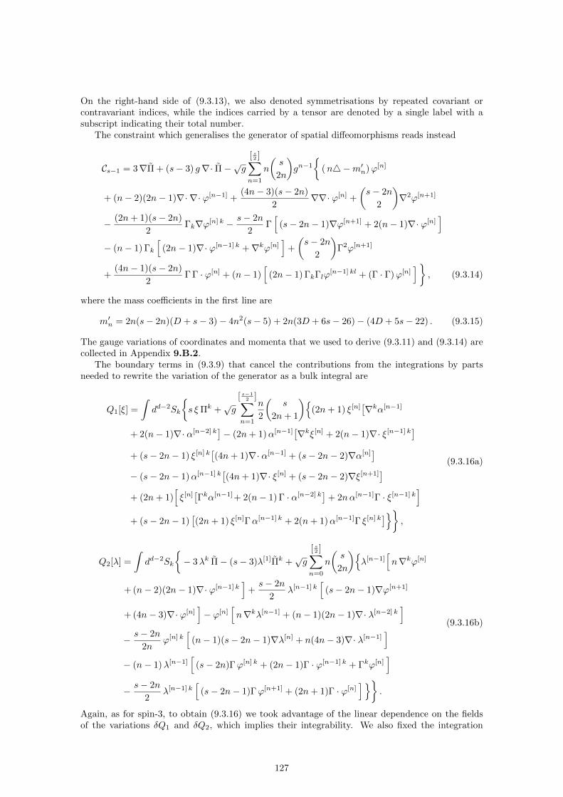
On the right-hand side of (9.3.13), we also denoted symmetrisations by repeated covariant orcontravariant indices, while the indices carried by a tensor are denoted by a single label with asubscript indicating their total number.

The constraint which generalises the generator of spatial diffeomorphisms reads instead

Cs−1 = 3∇Π + (s− 3) g∇· Π−√g[ s2 ]∑

n=1

n

(s

2n

)gn−1

(n4−m′n)ϕ[n]

+ (n− 2)(2n− 1)∇· ∇· ϕ[n−1] +(4n− 3)(s− 2n)

2∇∇· ϕ[n] +

(s− 2n

2

)∇2ϕ[n+1]

− (2n+ 1)(s− 2n)

2Γk∇ϕ[n] k − s− 2n

2Γ[

(s− 2n− 1)∇ϕ[n+1] + 2(n− 1)∇· ϕ[n]]

− (n− 1) Γk

[(2n− 1)∇· ϕ[n−1] k +∇kϕ[n]

]+

(s− 2n

2

)Γ2ϕ[n+1]

+(4n− 1)(s− 2n)

2Γ Γ · ϕ[n] + (n− 1)

[(2n− 1) ΓkΓlϕ

[n−1] kl + (Γ · Γ)ϕ[n]]

, (9.3.14)

where the mass coefficients in the first line are

m′n = 2n(s− 2n)(D + s− 3)− 4n2(s− 5) + 2n(3D + 6s− 26)− (4D + 5s− 22) . (9.3.15)

The gauge variations of coordinates and momenta that we used to derive (9.3.11) and (9.3.14) arecollected in Appendix 9.B.2.

The boundary terms in (9.3.9) that cancel the contributions from the integrations by partsneeded to rewrite the variation of the generator as a bulk integral are

Q1[ξ] =

∫dd−2Sk

s ξΠk +

√g

[ s−12 ]∑

n=1

n

2

(s

2n+ 1

)(2n+ 1) ξ[n]

[∇kα[n−1]

+ 2(n− 1)∇· α[n−2] k]− (2n+ 1)α[n−1]

[∇kξ[n] + 2(n− 1)∇· ξ[n−1] k

]+ (s− 2n− 1) ξ[n] k

[(4n+ 1)∇· α[n−1] + (s− 2n− 2)∇α[n]

]− (s− 2n− 1)α[n−1] k

[(4n+ 1)∇· ξ[n] + (s− 2n− 2)∇ξ[n+1]

]+ (2n+ 1)

[ξ[n][Γkα[n−1]+ 2(n− 1) Γ · α[n−2] k

]+ 2nα[n−1]Γ · ξ[n−1] k

]+ (s− 2n− 1)

[(2n+ 1) ξ[n]Γα[n−1] k + 2(n+ 1)α[n−1]Γ ξ[n] k

],

(9.3.16a)

Q2[λ] =

∫dd−2Sk

− 3λk Π− (s− 3)λ[1]Πk +

√g

[ s2 ]∑

n=0

n

(s

2n

)λ[n−1]

[n∇kϕ[n]

+ (n− 2)(2n− 1)∇· ϕ[n−1] k]

+s− 2n

2λ[n−1] k

[(s− 2n− 1)∇ϕ[n+1]

+ (4n− 3)∇· ϕ[n]]− ϕ[n]

[n∇kλ[n−1] + (n− 1)(2n− 1)∇· λ[n−2] k

]− s− 2n

2nϕ[n] k

[(n− 1)(s− 2n− 1)∇λ[n] + n(4n− 3)∇· λ[n−1]

]− (n− 1)λ[n−1]

[(s− 2n)Γϕ[n] k + (2n− 1)Γ · ϕ[n−1] k + Γkϕ[n]

]− s− 2n

2λ[n−1] k

[(s− 2n− 1)Γϕ[n+1] + (2n+ 1)Γ · ϕ[n]

].

(9.3.16b)

Again, as for spin-3, to obtain (9.3.16) we took advantage of the linear dependence on the fieldsof the variations δQ1 and δQ2, which implies their integrability. We also fixed the integration

127

constants to zero on the zero solution.8 The resulting Q1 and Q2 are the surface charges: in thefollowing we shall introduce boundary conditions on the canonical variables and on deformationparameters generating asymptotic symmetries. In section 9.3.3 we shall show how these conditionssimplify asymptotically (9.3.16) and we shall verify that the resulting spin-s charges are finite andnon-vanishing.

9.3.2 Boundary conditions and asymptotic symmetries

As in the spin-3 case, we derive boundary conditions on the canonical variables from the falloffat spatial infinity of the solutions of Fronsdal’s equation in a convenient gauge, adopting thesubleading branch. This is recalled in Appendix 9.C: in the coordinates (9.2.21), the relevantsolutions behave at spatial infinity (r →∞) as

ϕI1···Is = r3−d TI1···Is(xM ) +O(r1−d) , (9.3.17a)

ϕr···rI1···Is−k= O(r3−d−3k) , (9.3.17b)

where capital Latin indices denote again directions transverse to the radial one. The symmetricboundary tensor TI1···Is is a traceless conserved current :

∂JϕJI1···Is−1= ηJKϕJKI1···Is−2

= 0 . (9.3.18)

For s = 2 the fall-off conditions on hIJ and hrI agree with those proposed for non-linear Einsteingravity in eq. (2.2) of [129]. Our hrr decays instead faster at infinity; the mismatch can beinterpreted anyway as a radial gauge fixing, as discussed in sect. 2.1 of [63]. For d = 3, (9.3.17)also agrees with the boundary conditions in eq. (5.3) of [63], with the same provisos as thosediscussed for the spin-3 case in section 9.2.3.

From (9.3.17) one obtains the boundary conditions on half of the canonical variables:

ϕα1···αs = r3−d Tα1···αs +O(r1−d) , (9.3.19a)

ϕr···rα1···αs−k= O(r3−d−3k) , (9.3.19b)

αα1···αs−3= −2 r−d T000α1···αs−3

+O(r−d−2) , (9.3.19c)

αr···rα1···αs−3−k= O(r−d−3k) , (9.3.19d)

where Greek indices from the beginning of the alphabet denote angular coordinates on the d − 2sphere. The boundary conditions on the momenta are determined by making use of (9.3.17) in thedefinitions (9.3.7) and (9.3.8):

Πr···rα1···αs−k =

O(r−1−2(s−k)) , k = 2m− 2 ,

O(r−2(s−k)) , k = 2m− 1 ,(9.3.20a)

Πr···rα1···αs−3−k =

O(r2−2(s−k)) , k = 2m− 2 ,

O(r3−2(s−k)) , k = 2m− 1 ,(9.3.20b)

with m a positive integer. For arbitrary spin, the components actually contributing to the chargesare only Πrα1···αs−1 and Πrα1···αs−4 , whose dependence on the boundary current TI1···Is is detailed,respectively, in (9.E.10) and (9.E.13).

The deformation parameters that generate, via (9.3.9) and (9.3.10), gauge transformationspreserving the boundary conditions behave at spatial infinity as

ξα1···αs−1 = χα1···αs−1 +O(r−2) , ξr···rα1···αs−1−k = O(rk) , (9.3.21a)

λα1···αs−2 = −2 r χ0α1···αs−2r +O(r−1) , λr···rα1···αs−2−k = O(r1+k) , (9.3.21b)

8The latter operation requires some care in d = 3, where it is customary to assign the negative energy M = −1/8Gto AdS3. To this end, one can either introduce an integration constant in (9.3.16) for s = 2 or declare that thevacuum is identified by a corresponding non-trivial TIJ in the boundary conditions specified below in (9.3.17).This modification of the background metric does not affect the final expression for the charges (9.3.24), since itintroduces only corrections that vanish at the boundary. It however allows a direct match with the conventions ofthe Chern-Simons formulation [142,60] (see e.g. (9.3.26)).

128

where χI1···Is−1 is a traceless conformal Killing tensor for the Minkowski metric ηIJ [99], satisfying

∂(I1χI2···Is) −s− 1

d+ 2(s− 2)− 1η(I1I2 ∂ · χI3···Is) = 0 , ηJKχ

JKI1···Is−3 = 0 . (9.3.22)

The conditions (9.3.21) and (9.3.22) can be derived as for the spin-3 case discussed in section 9.2.4.We refrain from detailing the analysis of asymptotic symmetries also for arbitrary spin becauseonly the information on the leading terms displayed in (9.3.21) is relevant for the computationof charges. The existence of non-trivial asymptotic symmetries – in which part of the subleadingterms in (9.3.21) are fixed in order to preserve (9.3.17) – is again guaranteed by the existenceof traceless Killing tensors for the AdS background (see e.g. [211, 26, 15]). The latter solve theequations

∇(µ1Λµ2···µs) = 0 , Λρρµ1···µs−3

= 0 , (9.3.23)

and generate gauge transformations preserving the vacuum solution ϕµ1···µs = 0, which is triviallyincluded in the boundary conditions (9.3.17).

9.3.3 Charges

The computation of asymptotic charges for arbitrary integer spin s is performed following similarsteps to those for the spin-3 case, although with the contribution of terms that vanish for s = 3, inboth charges and momenta. Using the coordinates (9.2.21) and the asymptotic behaviour of thecanonical variables (9.3.19)–(9.3.21) one sees that the only terms that contribute to (9.3.16) at theboundary are

limr→∞

Q1[ξ] = s

∫dd−2x

ξΠr +

√g

[ s−12 ]∑

n=1

n

2

(s− 1

2n

)ξ[n]

[∇rα[n−1] − Γrα[n−1]

+ 2(n− 1)∇ · α[n−2] r]− α[n−1]

[∇rξ[n] + 2(n− 1)∇ · ξ[n−1] r

] (9.3.24a)

and

limr→∞

Q2[λ] =

∫dd−2x

− (s− 3)λ[1]Πr+

√g

[ s2 ]∑

n=0

n

(s

2n

)λ[n−1]

[(n− 2)(2n− 1)∇· ϕ[n−1] r

+n∇rϕ[n]]− ϕ[n]

[n∇rλ[n−1] + (n− 1)

((2n− 1)∇ · λ[n−2] r + Γrλ[n−1]

)], (9.3.24b)

where, as in (9.2.41), all omitted indices (including those involved in traces) take values in thed− 2 sphere at infinity.

The explicit form of these contributions in terms of the boundary current and of the boundaryconformal Killing tensor that generate asymptotic symmetries is (see Appendix 9.E for details)

limr→∞

Q1 = C

∫dd−2x

[(s−1)/2]∑n=0

(s− 1

2n

)(χ[n])αs−2n−1(T [n])0αs−2n−1 , (9.3.25a)

limr→∞

Q2 = C

∫dd−2x

[s/2]∑n=1

(s− 1

2n− 1

)(χ[n−1])0αs−2n(T [n])αs−2n

, (9.3.25b)

with C = s(d + 2s− 5). For better clarity, we specified the number of angular indices omitted in(9.3.24), and we recall that traces are understood to follow from contractions with the metric gαβon the d− 2 sphere. Taking advantage of the trace constraints on both TIs and χIs−1 , the sum ofthe two charges partly covariantises in the indices transverse to the radial direction as in (9.2.43):

Q ≡ limr→∞

(Q1 +Q2) = C

∫dd−2x

s−1∑n=0

(s− 1

n

)χ

n︷︸︸︷0···0αs−n−1T0···0︸︷︷︸

n+1

αs−n−1

= s(d+ 2s− 5)

∫dd−2xχIs−1T0Is−1

.

(9.3.26)

129

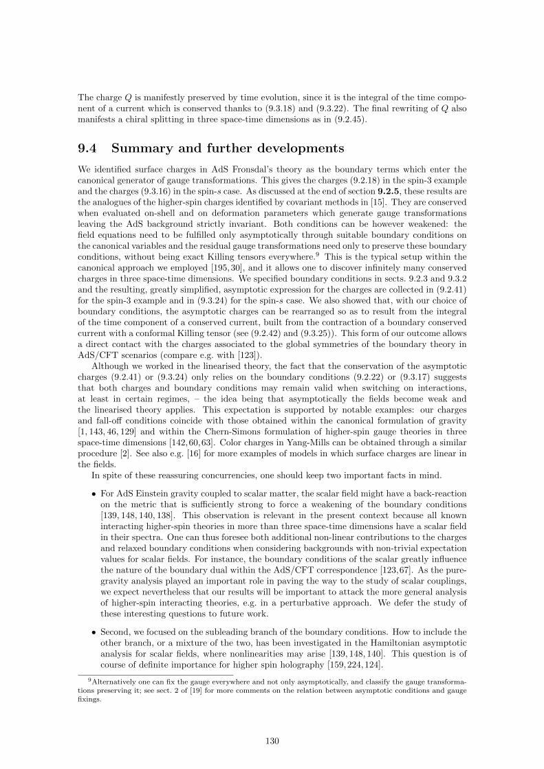
The charge Q is manifestly preserved by time evolution, since it is the integral of the time compo-nent of a current which is conserved thanks to (9.3.18) and (9.3.22). The final rewriting of Q alsomanifests a chiral splitting in three space-time dimensions as in (9.2.45).

9.4 Summary and further developments

We identified surface charges in AdS Fronsdal’s theory as the boundary terms which enter thecanonical generator of gauge transformations. This gives the charges (9.2.18) in the spin-3 exampleand the charges (9.3.16) in the spin-s case. As discussed at the end of section 9.2.5, these results arethe analogues of the higher-spin charges identified by covariant methods in [15]. They are conservedwhen evaluated on-shell and on deformation parameters which generate gauge transformationsleaving the AdS background strictly invariant. Both conditions can be however weakened: thefield equations need to be fulfilled only asymptotically through suitable boundary conditions onthe canonical variables and the residual gauge transformations need only to preserve these boundaryconditions, without being exact Killing tensors everywhere.9 This is the typical setup within thecanonical approach we employed [195, 30], and it allows one to discover infinitely many conservedcharges in three space-time dimensions. We specified boundary conditions in sects. 9.2.3 and 9.3.2and the resulting, greatly simplified, asymptotic expression for the charges are collected in (9.2.41)for the spin-3 example and in (9.3.24) for the spin-s case. We also showed that, with our choice ofboundary conditions, the asymptotic charges can be rearranged so as to result from the integralof the time component of a conserved current, built from the contraction of a boundary conservedcurrent with a conformal Killing tensor (see (9.2.42) and (9.3.25)). This form of our outcome allowsa direct contact with the charges associated to the global symmetries of the boundary theory inAdS/CFT scenarios (compare e.g. with [123]).

Although we worked in the linearised theory, the fact that the conservation of the asymptoticcharges (9.2.41) or (9.3.24) only relies on the boundary conditions (9.2.22) or (9.3.17) suggeststhat both charges and boundary conditions may remain valid when switching on interactions,at least in certain regimes, – the idea being that asymptotically the fields become weak andthe linearised theory applies. This expectation is supported by notable examples: our chargesand fall-off conditions coincide with those obtained within the canonical formulation of gravity[1, 143, 46, 129] and within the Chern-Simons formulation of higher-spin gauge theories in threespace-time dimensions [142,60,63]. Color charges in Yang-Mills can be obtained through a similarprocedure [2]. See also e.g. [16] for more examples of models in which surface charges are linear inthe fields.

In spite of these reassuring concurrencies, one should keep two important facts in mind.

• For AdS Einstein gravity coupled to scalar matter, the scalar field might have a back-reactionon the metric that is sufficiently strong to force a weakening of the boundary conditions[139, 148, 140, 138]. This observation is relevant in the present context because all knowninteracting higher-spin theories in more than three space-time dimensions have a scalar fieldin their spectra. One can thus foresee both additional non-linear contributions to the chargesand relaxed boundary conditions when considering backgrounds with non-trivial expectationvalues for scalar fields. For instance, the boundary conditions of the scalar greatly influencethe nature of the boundary dual within the AdS/CFT correspondence [123,67]. As the pure-gravity analysis played an important role in paving the way to the study of scalar couplings,we expect nevertheless that our results will be important to attack the more general analysisof higher-spin interacting theories, e.g. in a perturbative approach. We defer the study ofthese interesting questions to future work.

• Second, we focused on the subleading branch of the boundary conditions. How to include theother branch, or a mixture of the two, has been investigated in the Hamiltonian asymptoticanalysis for scalar fields, where nonlinearities may arise [139, 148, 140]. This question is ofcourse of definite importance for higher spin holography [159,224,124].

9Alternatively one can fix the gauge everywhere and not only asymptotically, and classify the gauge transforma-tions preserving it; see sect. 2 of [19] for more comments on the relation between asymptotic conditions and gaugefixings.

130

Even when the surface integrals are determined by the linear theory without nonlinear correc-tions, the interactions play a crucial role in the study of the asymptotic symmetry algebra. Thiscan be seen in many ways. For instance, the Poisson bracket of charges, that is their algebra, canbe derived from their variation under gauge transformations preserving the boundary conditions.However, as shown in sects. 9.2.4 and 9.3.2, in the linearised theory the charges are left invariantby asymptotic symmetries in all space-time dimensions except d = 3 (but there the variation onlygives rise to a central term in the algebra). The fact that one must include interactions in order toderive the asymptotic symmetry algebra is not a higher-spin feature, though. In general relativity,although the surface charges are correctly reproduced by the linear theory, one has to know howthe metric transforms under diffeomorphisms (and not only under their linearised version) in orderto obtain the algebra of asymptotic symmetries (see e.g. [46,45]). A similar phenomenon arises forcolor charges in Yang-Mills theory.

This mechanism is also clearly displayed by the comparison between sects. 9.2.4 and 9.3.2and the similar analysis performed in d = 3 in [63], where the effect of gravitational couplingsand of the self-interactions of higher-spin fields manifests itself in the non-linear variations of thelinear charges. Similarly, higher-spin Lie algebras emerge when considering commutators of gaugetransformations induced by cubic vertices and restricted to gauge parameters that at linearisedlevel leave the AdS background invariant [41, 166]. It will be interesting to compare this analysiswith that of surface charges developed in this and the related papers [15,65]. Note that the analysisof asymptotic symmetries in [67,193] also involves ingredients that go beyond the linearised regime,like the full knowledge of the higher-spin gauge algebra on which the bulk theory is built upon.

Let us finally point out other possible extensions. Our results apply to any space-time dimensionbut they do not cover all possible bosonic higher-spin gauge theories. When d > 4, mixed symmetryfields (see e.g. [58] for a review) are a new possibility. In AdS they loose almost all gauge symmetriesthey display in flat space, but the remaining ones should give rise to conserved charges generalisingthose discussed in this chapter. An analysis along the lines we followed for symmetric fields maystart from the actions of [59], which constitutes at present the closest generalisation of the Fronsdalaction known in closed form. Partially massless fields [86,89,232] are other gauge fields which canbe defined on constant curvature backgrounds and have less gauge symmetry than Fronsdal’s fields.This generalisation comprises gauge fields that do not propagate unitarily on AdS. It would beinteresting to investigate whether one can define in this case boundary conditions allowing fornon-trivial residual symmetries and supporting consequently non-trivial conserved charges. Howsuch charges, if they exist, would fit with the classical instability of the partially massless theorieswould also deserve to be understood.

131

Appendix

9.A Notation and conventions

We adopt the mostly-plus convention for the space-time metric and we denote by d the dimensionof space-time. The AdS radius L is defined as

[∇µ , ∇ν ]Vρ =1

L2(gνρVµ − gµρVν) . (9.A.1)

In the static coordinates (9.2.2) the spatial metric satisfies (9.A.1) as the full space-time metricprovided one substitutes everywhere µ, ν → i, j.

We distinguish between four types of indices, depending on whether the time and/or radial co-ordinates are included or not. Greek letters from the middle of the alphabet include all coordinates,small Latin letters include all coordinates except t, capital Latin letters include all coordinates ex-cept r, while Greek letters from the beginning of the alphabet denote angular coordinates on theunit d− 2 sphere. In summary:

µ, ν, . . . ∈ t, r, φ1, . . . , φd−2 , i, j, . . . ∈ r, φ1, . . . , φd−2 ,

I, J, . . . ∈ t, φ1, . . . , φd−2 , α, β, . . . ∈ φ1, . . . , φd−2 . (9.A.2)

Indices between parentheses (or square brackets) are meant to be (anti)symmetrised with weightone, i.e. one divides the (anti)symmetrised expression by the number of terms that appear in it,so that the (anti)symmetrisation of a (anti)symmetric tensor is a projection.

In section 9.2 omitted indices denote a trace, whose precise meaning depends on the context:in covariant expressions a contraction with the full space-time metric gµν is understood, whilecontractions with the spatial metric gij or with the boundary metric gIJ are understood in formulaedisplaying the corresponding types of indices.

In most of section 9.3 we omit instead all indices: in linear expressions we elide all free indices,which are meant to be symmetrised, while in expressions quadratic in the fields omitted indicesare meant to be contracted. In order to avoid ambiguities, however, in some terms we displayexplicitly a pair of contracted indices, continuing to elide the remaining ones. Traces, symmetrisedgradients and divergences are denoted by

ϕ[n] ≡ ϕµ1···µs−2nλ1···λn

λ1···λn , ∇ϕ ≡ ∇(µ1ϕµ2···µs+1) , ∇ · ϕ ≡ ∇λϕλµ1···µs−1 . (9.A.3)

We recalled here covariant expressions as an example, but contractions may also run only overspatial or transverse indices depending on the context. Similar shortcuts are adopted to denotesymmetrisations or contractions with the “extrinsic” Christoffel symbol (9.2.8):

Γϕ ≡ Γ00(i1ϕi2···is+1) , Γ · ϕ ≡ gklΓ0

0kϕli1···is−1. (9.A.4)

In Appendix 9.C and in some expressions of section 9.3 we reinstate indices with the followingconvention: repeated covariant or contravariant indices denote a symmetrisation, while a couple ofidentical covariant and contravariant indices denotes as usual a contraction. Moreover, the indicescarried by a tensor are substituted by a single label with a subscript indicating their total number.For instance, the combinations in (9.A.3) may also be presented as

ϕ[n] = ϕµs−2n , ∇ϕ = ∇µϕµs , ∇ · ϕ ≡ ∇λϕλµs−1 . (9.A.5)

Finally, our Hamiltonian conventions are [q, p] = 1 and F = [F,H].

132

9.B Hamiltonian form of Fronsdal’s action

This appendix collects some additional details on the rewriting of spin-3 Fronsdal’s action inHamiltonian form and on the derivation of first class constraints in the spin-s case.

9.B.1 Spin 3

Integrating by parts the time derivative, one can eliminate on any static background all terms withNi and Nij which appear in the expansion in components of the Fronsdal action (9.2.1). This isbecause the lapse does not depend on time, so that this step of the computation works as in flatspace. Eliminating time derivatives from Ni and Nij , however, does not suffice to identify themas Lagrange multipliers: one must also verify that they enter linearly the action. The cancellationof the quadratic terms requires instead that the metric (9.2.2) be of constant curvature since ingeneral

S = SFronsdal +

∫d dx

3√g

2f

f

(R0ij

0 − 1

L2gij

)(2Nkϕijk −N iϕj − gijNα

)+ 4

[N ij [∇k ,∇i]Njk +

d

L2

(NijN

ij +N2)−R0ij

0(N i

kNjk + 2N ijN + gijN2

)]−[N i[∇j ,∇i]N j +

2d

L2NiN i −R0ij

0(3N iN j + gijNiN i

)],

(9.B.1)

where SFronsdal is the same action as (9.2.7), with the same H, Ci and Cij , while Rµνρσ denotes

the Riemann tensor of the background. In obtaining this result we used only

Γ000 = Γ0

ij = Γi0j = 0 , Γi00 = f2gijΓ00j (9.B.2)

together with (9.2.8), which hold for a generic static metric.The first line in (9.B.1) would provide an additional contribution to the constraints, that

vanishes on a constant curvature background on account of

Rµνρσ = − 1

L2(gµρgνσ − gµσgνρ) . (9.B.3)

The second and third lines must instead vanish and this requires (9.B.3). The missing cancellationof the terms quadratic in Ni and Nij is the counterpart of the loss of the gauge symmetry (9.2.13)on arbitrary backgrounds. Correspondingly, in the canonical formalism one obtains first classconstraints only on constant curvature backgrounds.

9.B.2 Arbitrary spin

In order to reconstruct the canonical generator of gauge transformations (9.3.9) by integrating(9.3.10), one has to reconstruct the gauge transformations of the canonical variables from Fronsdal’scovariant gauge transformation (9.3.3). To this end, one has to set a map between the componentsof the covariant gauge parameter Λµ1···µs−1

and the deformation parameters ξi1···is−1and λi1···is−2

that enter (9.3.9). To obtain dimensions compatible with the action (9.3.6) and to agree with thespin-3 example, we choose

ξi1···is−1 = Λi1···is−1 , λi1···is−2 = 2f−1Λ0 i1···is−2 . (9.B.4)

The other components of the covariant gauge parameter are not independent from the ones abovedue to Fronsdal’s constraint.

Combining (9.3.3) with (9.B.4) one obtains the following variations for the canonical variablesand their traces:

δϕ[n] = 2n∇· ξ[n−1] + (s− 2n)∇ξ[n] , (9.B.5a)

δα[n] = −(2n+ 3)∇· λ[n] − (s− 2n− 3)∇λ[n+1] . (9.B.5b)

133

The gauge transformations of the Lagrange multipliers and their traces are obtained in a similarfashion:

δN [n] = ξ[n] + nf∇· λ[n−1] − Γ · λ[n−1]

+s− 2n− 1

2f∇λ[n] − Γλ[n]

, (9.B.6a)

δN [n] = λ[n] + 2fn∇· ξ[n] − (2n+ 1) Γ · ξ[n]

+ (s− 2n− 2)f

∇ξ[n+1] − 2 Γ ξ[n+1]

.

(9.B.6b)

Substituting (9.B.5) and (9.B.6) in the definitions of the momenta (9.3.7) and (9.3.8) one obtains

δΠ =√g

[ s2 ]∑

n=0

(s

2n

)gn

(n− 1)

(s− 2n

2

)∇2λ[n] + n

[(n− 1)(2n− 1)∇· ∇· λ[n−2]

+

(n4− n(s− 2n)(D + s− 2n− 3) + (2n− 1)(D + 2s− 2n2 + 4n− 8)

L2

)λ[n−1]

+(4n− 3)(s− 2n)

2∇∇· λ[n−1] +

s− 2n

2Γ(

(s− 2n− 1)∇λ[n] + (2n+ 1)∇· λ[n−1])

+ (n− 1) Γk

((s− 2n)∇λ[n−1] k + (2n− 1)∇· λ[n−2] k +∇kλ[n−1]

)], (9.B.7)

δΠ =√g

[ s−12 ]∑

n=1

n

2

(s

2n+ 1

)gn−1

2(n− 1)(2n+ 1)∇· ∇· ξ[n−1]

+ (2n+ 1)

[4− (s− 2n− 1)(D + s− 2n− 4) + 2(D + 2s− 2n2 + 3n− 7)

L2

]ξ[n]

+ (s− 2n− 1)[

(4n+ 1)∇∇· ξ[n] + (s− 2n− 2)∇2ξ[n+1]]

− (s− 2n− 1) Γ[

(s− 2n− 2)∇ξ[n+1] + 2(n+ 1)∇· ξ[n]]

− (2n+ 1) Γk

[(s− 2n− 1)∇ξ[n] k + 2n∇· ξ[n−1] k +∇kξ[n]

]. (9.B.8)

To derive (9.B.7) and (9.B.8) we used identities that are valid only on a constant-curvature space-time, as

∇iΓ00j + Γ0

0iΓ00j =

1

L2gij (9.B.9)

which follows from (9.B.3). We also commuted covariant derivatives using, for instance,

[∇k,∇ ]λ[n−1] k = − 1

L2

(D + s− 2n− 3)λ[n−1] − (s− 2n− 1)gλ[n]

. (9.B.10)

134

9.C Covariant boundary conditions

In this appendix we recall the falloff at the boundary of AdSd of the solutions of Fronsdal’s equationsof motion (see also e.g. [182,177,159]). To achieve this goal we partially fix the gauge freedom, andwe also exhibit the fall-off conditions on the parameters of the residual gauge symmetry (whichinclude the traceless Killing tensors of AdSd).

We set the AdS radius to L = 1 and we work in the Poincare patch parameterised as

ds2 =1

z2

(dz2 + ηIJdx

IdxJ)

(9.C.1)

In these coordinates the spatial boundary is at z → 0. All results can be easily translated in thecoordinates (9.2.21) used in the main body of the text (z = 1/r), in which the boundary is atr → ∞. We denote by capital Latin indices all directions transverse to the radial one (includingtime).

9.C.1 Falloff of the solutions of the free equations of motion

We wish to study the space of solutions of the Fronsdal equation in AdSd [117, 47] which, in theindex-free notation of section 9.3, reads

ϕ− s ∇(∇ · ϕ− s− 1

2∇ϕ[1]

)− s2 + (d− 6)s− 2(d− 3)

L2ϕ− 2

L2

(s

2

)g ϕ[1] = 0 (9.C.2)

To this end it is convenient to partially fix the gauge freedom (9.3.3) by imposing ∇ · ϕ = 0 andϕ[1] = 0. This gauge is reachable on-shell,10 as it is proven e.g. in sect. 3.1 of [182]. The previousstatement amounts to say that the space of solutions (modulo gauge transformations) of (9.C.2)is equivalent to the space of solutions of the Fierz system[

−(s2 + (d− 6)s− 2(d− 3)

)]ϕ = 0 , (9.C.3a)

∇ · ϕ = 0 , (9.C.3b)

ϕ[1] = 0 , (9.C.3c)

which also describes the propagation of a free massless particle of spin s in the AdSd background[175]. Actually the conditions (9.C.3b) and (9.C.3c) do not fix completely the gauge: the Fierzsystem admits gauge transformations still of the form δϕ = s∇Λ, but with gauge parametersconstrained as

[− (s− 1)(d+ s− 3) ] Λ = 0 , (9.C.4a)

∇ · Λ = 0 , (9.C.4b)

Λ[1] = 0 . (9.C.4c)

To analyse the falloff at the boundary of the solutions of the conditions (9.C.3), one has to treatseparately field components with a different number of indices along the z direction. We denotethem as

ϕzkIs−k≡ ϕz···z I1···Is−k

. (9.C.5)

The divergence constraint (9.C.3b) then gives

(z∂z − (d− 2))ϕzµs−1+ z ∂IϕIµs−1

= 0 , (9.C.6)

where Greek letters denote indices that take values in all space-time dimensions (including z). Thetrace constraint (9.C.3c) gives instead

ϕzzµs−2 + ηIJϕIJµs−2 = 0 . (9.C.7)

10In flat space one easily sees that one can reach the gauge ∂ · ϕ = ϕ[1] = 0 only on-shell: imposing ϕ[1] = 0implies ∂ · ξ = 0, but the divergence of the field, which now transforms as δ∂ · ϕ = ξ, is not divergenceless. In thegauge ϕ[1] = 0 the solutions of the equations of motion satisfy however ϕ− s ∂∂ · ϕ = 0; taking a divergence oneobtains ∂ · ∂ · ϕ = 0 allowing to reach the desired gauge.

135

Using (9.C.6) and (9.C.7) the components of the equation of motion (9.C.3a) read[z2∂2

z − (d− 2(s− k + 1)) z∂z − (d+ k − 3)(2s− k − 2)]ϕzkIs−k

+ z2ϕzkIs−k− 2(s− k) z ∂Iϕzk+1Is−k−1

+ (s− k)(s− k − 1) ηIIϕzk+2Is−k−2= 0 ,

(9.C.8)

where now = ηIJ∂I∂J and repeated covariant or contravariant indices denote a symmetrisation,see e.g. (9.A.5).

Eq. (9.C.6) implies ϕzkIs−k∼ z∆+k; substituting this ansatz in (9.C.8) the terms in the second

line are subleading for z → 0 and the first line vanishes provided that

ϕz···z I1···Is−k∼ z∆±+ k with

∆+ = d− 3

∆− = 2− 2s. (9.C.9)

For s = 0 one recovers the asymptotic behaviour of the conformally coupled scalar of mass m2 =−2(d − 3) that enters the Vasiliev equations. For higher spins the subleading ∆+ branch givesthe boundary conditions usually considered within the AdS/CFT correspondence [123, 193] andadopted in the text, while the ∆− branch has been considered in a holographic setup in [159,224,124].

9.C.2 Residual gauge symmetry

The constraints (9.C.4) force the gauge parameters to have a precise fall off at the boundary, whichcan be determined as above. The divergence and trace constraints give again

(z∂z − (d− 2)) Λzµs−2+ z ∂IΛIµs−2

= 0 , (9.C.10a)

Λzzµs−3 + ηIJΛIJµs−3 = 0 . (9.C.10b)

Eq. (9.C.10a) implies ΛzkIs−k−1∼ zΘ+k and using the relations above in (9.C.4a) one gets[

z2∂2z − (d− 2(s− k)) z∂z − (d+ k − 1)(2s− k − 2) + z2

]ΛzkIs−k−1

− 2(s− k − 1) z∂IΛzk+1Is−k−2+ (s− k − 1)(s− k − 2) ηIIΛzk+2Is−k−3

= 0 .(9.C.11)

This equation is identical to (9.C.8), apart from the shift s→ s− 1 and a modification in the massterms which implies that the first line vanishes asymptotically when

ξz···z I1···Is−k−1∼ zΘ±+ k with

Θ+ = d− 1

Θ− = 2− 2s. (9.C.12)

We solved a second order equation and, as a result, we obtained two allowed asymptotic be-haviours for the gauge parameters. On the contrary, the Killing equation (9.3.23) is of first orderand Killing tensors admit only a given boundary falloff. To fix it, notice that the AdS backgroundis left invariant by the same set of gauge transformations in both Fronsdal’s and Fierz’s formu-lations: the gauge parameters are traceless in both setups and a traceless Killing tensor is alsodivergenceless thanks to

gαα∇αΛαµs−2= −s− 2

2gαα∇µΛααµs−2 = 0 . (9.C.13)

Traceless Killing tensors must therefore display one of the two boundary behaviours above. TheKilling equation ∇µξµs−1

= 0 branches in components as

[z∂z + (2s− k − 2)] ΛzkIs−k−1=s− k − 1

k + 1

[−z ∂IΛzk+1Is−k−2

+ (s− k − 2)ηIIΛzk+2Is−k−3

].

(9.C.14)The right-hand side is subleading, and one thus sees that Killing tensors belong to the Θ− branchof (9.C.12).

136

9.C.3 Initial data at the boundary

In this subsection we recall the constraints on the initial data at the boundary imposed by diver-gence and trace constraints, and how the number of independent components is further reduced bythe residual gauge symmetry. To this end we denote the leading contributions in the ∆+ branchby

ϕIs = z∆+TIs(xJ) +O(z∆++2

), (9.C.15a)

ϕzkIs−k= z∆++k t

(k)Is−k

(xJ) +O(z∆++k+2

), 1 ≤ k ≤ s , (9.C.15b)

and the leading contributions in the ∆− branch by

ϕIs = z∆−ΦIs(xJ) +O(z∆−+2

), (9.C.16a)

ϕzkIs−k= z∆−+k φ

(k)Is−k

(xJ) +O(z∆−+k+2

), 1 ≤ k ≤ s . (9.C.16b)

The subleading terms can be expressed in terms of the leading ones via the field equations (seee.g. [177]).

The tensors TIs and ΦIs are boundary fields of conformal dimensions, respectively, ∆c = d+s−3and ∆s = 2 − s. They thus correspond to the conserved currents and shadow fields of [176].11

Note that ∆c + ∆s = d− 1, i.e. the sum of conformal dimensions is equal to the dimension of theboundary. Therefore the coupling ΦIsTIs is conformally invariant. In the AdS/CFT jargon ΦIs isa source and TIs is the corresponding vev.

The trace constraint (9.C.7) then implies that all tensors on the right-hand side of (9.C.15) and(9.C.16) are traceless, since the trace of ϕzkIs−k

is subleading with respect to the traceless part.The divergence constraint (9.C.6) has instead different consequences in the two branches: in the∆+ branch of vevs one obtains

∂ · TIs−1 = 0 , (9.C.17a)

t(k+1)Is−k−1

= −1

k∂ · t(k)

Is−k−1, 1 ≤ k ≤ s , (9.C.17b)

while in the ∆− branch of sources one obtains

φ(k+1)Is−k−1

=1

d+ 2s− k − 5∂ · φ(k)

Is−k−1, 0 ≤ k ≤ s , (9.C.18)

where φ(0)Is≡ ΦIs and where divergences are meant to involve sums only over indices transverse to

z. Eq. (9.C.17a) shows that, as expected from its conformal weight, T is a conserved current. Upto this point t(1) is instead an arbitrary tensor (but we still have to consider the residual gaugesymmetry), while all other tensors in (9.C.15) are not independent. In the other branch the onlyindependent tensor is instead Φ, whose number of independent components is the same as thoseof T plus t(1).

The residual gauge symmetry is generated by

ΛzkIs−k−1= zΘ++k ξ

(k)Is−k−1

(xJ) +O(zΘ++k+2

), (9.C.19)

orΛzkIs−k−1

= zΘ−+k ε(k)Is−k−1

(xJ) +O(zΘ−+k+2

). (9.C.20)

In the following we shall often denote ξ(0) by ξ and ε(0) by ε. As for the fields, the trace constraint(9.C.10b) imposes that all tensors in (9.C.19) and (9.C.20) be traceless. For gauge parameters the

11If one performs a dilatation xµ → λxµ the tensor ϕI1···Is transforms as ϕI′s = λ−sϕIs , while on the right-hand

side of (9.C.15a) or (9.C.16a) one has z′∆± = λ∆±z∆± . As a result, T and Φ must transform as TI′s = λ−(∆++s)TIsand ΦI′s = λ−(∆−+s)ΦIs , from where one reads the conformal dimensions. To obtain a direct matching between the

exponents ∆± and the conformal dimensions, one can contract all indices with the (inverse) vielbein eµM = z−1 δµM

as e.g. in [159].

137

divergence constraint (9.C.10a) has instead the same form in both branches:

ξ(k+1)Is−k−2

= − 1

k + 2∂ · ξ(k)

Is−k−2, 0 ≤ k ≤ s− 1 , (9.C.21a)

ε(k+1)Is−k−2

=1

d+ 2s− k − 5∂ · ε(k)

Is−k−2, 0 ≤ k ≤ s− 1 . (9.C.21b)

This means that only the tensors ξIs−1 and εIs−1 are independent.The components of the field transform as

δϕzkIs−k= k

[∂z +

2s− k − 1

z

]Λzk−1Is−k

+ (s− k)

[∂IΛzkIs−k−1

− s− k − 1

zηIIΛzk+1Is−k−2

].

(9.C.22)In the Θ+ branch the first contribution is leading and gives

δϕzkIs−k= k(d+ 2s− 3)zd−3+kξ

(k−1)Is−k

+O(zd−1+k) . (9.C.23)

These gauge transformations act naturally on vevs, where they induce

δTIs = 0 , δt(1)Is−1

= (d+ 2s− 3)ΛIs−1. (9.C.24)

The tensor t(1) is thus a Stueckelberg field that can be eliminated using the residual symmetrygenerated by ξ and the solution is fully specified by the conserved current T .

In the Θ− branch the coefficient of the leading contribution vanishes, and one obtains

δϕzkIs−k=

z2−2s+k

d+ 2s− 5

[kε(k−1)

Is−k+ (s− k)(d+ 2(s− k)− 5) ∂Iε

(k)Is−k−1

− (s− k)(s− k − 1)(d+ 2s− k − 5) ηIIε(k+1)Is−k−2

]+O(z4−2s+k) ,

(9.C.25)

where we used the second-order equation (9.C.11) to express the subleading contributions inΛzk−1Is−k

in terms of the leading ones. These gauge transformations act naturally on sources,where they induce

δΦIs = s ∂IεIs−1 −s(s− 1)

(d− 1) + 2(s− 2)ηII∂ · εIs−2

(9.C.26)

and similar transformations on the φ(k) = φ(k)(Φ). To obtain (9.C.26) we used (9.C.21b) toeliminate ε(1). This gauge freedom reduces the number of independent components of ΦIs suchthat it becomes identical to that of the conserved current TIs . Moreover, the gauge transformations(9.C.26) leave invariant the coupling ΦIsTIs .

To summarise, the solutions of the field equations are specified asymptotically either by atraceless and conserved current TIs or by a traceless tensor ΦIs subjected to the gauge symmetry(9.C.26). These tensors enter the components transverse to z as in (9.C.15a) and (9.C.16a), whileall other components of the spin-s field are expressed in terms of them via the field equations (orset to zero by the residual gauge symmetry (9.C.22)).

138

9.D Conformal Killing tensors

In this appendix we recall the structure of the general solution of the conformal Killing equations(9.3.22) and we present it explicitly in the rank-2 case. We also prove the identities (9.2.34) and(9.2.38), that we used in the analysis of asymptotic symmetries in the spin-3 example.

General solution of the rank-2 conformal Killing equation

When d − 1 > 2, the solutions of the conformal Killing tensor equation (9.3.22) are in one-to-one correspondence with rectangular traceless Young tableaux with two rows of s− 1 boxes ind + 1 dimensions [99], that we denote by s, s. For instance, a generic conformal Killing vector,vI = aI−ωI|JxJ +λxI +bK

(2xIx

K − δIKx2), can be cast in the form vI = ΦMV

M |N ΨIN , where

underlined indices take value in the (d+ 1)-dimensional ambient space R2,d−1 and

V I|J =

0 2bJ λ−2bI ωI|J −aI−λ aJ 0

, ΦI =

−x2/2xI1

, ΨIJ =

−xIδIJ0

. (9.D.1)

A similar characterisation of traceless conformal Killing tensors exists for any value of the rank [99].In particular, the pattern of tensors in d− 1 dimensions that specify the solution follows from thedecomposition of a traceless s, s tensor in d+ 1 dimensions (using the branching rules discussede.g. in § 8.8.A of [20]). In the rank-2 case one obtains

2, 2o(d+1) = (2, 2+ 2 2, 1+ 3 2+ 1, 1+ 2 1+ 1)o(d−1) . (9.D.2)

Correspondingly, the general solution of (9.2.30) is

χIJ = aIJ +

(b(IxJ) −

1

d− 1ηIJ b · x

)+ ωIJ|K x

K + λ

(xIxJ −

1

d− 1ηIJ x

2

)+ ρK|(IxJ)x

K +

(2 cK(IxJ)x

K − cIJ x2 − 2

d− 1ηIJcKLx

KxL)

+ ΩIJ|KL xKxL

+

(2 bKxIxJx

K− b(IxJ)x2 − 1

d− 1ηIJ(b · x)x2

)+(2 ωKL|(IxJ)x

KxL+ ωIJ|KxKx2

)+ cKL

(4xIxJx

KxL − 4 δK(IxJ)xLx2 + δKIδ

LJ x

4). (9.D.3)

All tensors in this expression are irreducible and traceless, so that e.g. ωIJ|K is symmetric in itsfirst two indices and satisfies ω(IJ|K) = 0.

When d− 1 = 2, the general solution depends instead on two chiral functions for any value ofthe rank. Introducing the light-coordinates x± = t± φ, eqs. (9.3.22) are solved by

χ+···+ = χ(x+) , χ+···+−···− = 0 , χ−···− = χ(x−) . (9.D.4)

Proof of eqs. (9.2.34) and (9.2.38)

We wish to prove that the rank-2 conformal Killing equation (9.2.30) implies the identities (9.2.34)and (9.2.38), which entail the cancellation of the first two subleading orders in δϕIJK . The followingproof is independent on the space-time dimension, but when d > 3 one could also verify theseidentities by acting with the differential operators they involve on (9.D.3).

As a first step, one can act with a derivative on the conformal Killing equation, and rewritethe result as follows

0 = ∂M

(∂(IχJK) −

2

d+ 1η(IJ ∂ · χK)

)= 2

(∂(M∂IχJK) −

2

d+ 1η(MI ∂J∂ · χK)

)− ∂(I∂JχK)M −

1

d+ 1

(η(IJ|∂M∂ · χ|K) − 2 ηM(I∂J∂ · χK) − η(IJ∂K)∂ · χM

).

(9.D.5)

The first term on the right-hand side vanishes since it is the symmetrisation of the left-hand side.As a result, one discovers that the second line vanishes as well.

139

To prove (9.2.34) one needs another identity obtained in a similar fashion:

0 = 3 ∂M∂N

(∂(IχJK) −

2

d+ 1η(IJ ∂ · χK)

)= 10

(∂(M∂N∂IχJK) −

2

d+ 1η(MN ∂I∂J∂ · χK)

)− ∂I∂J∂KχMN (9.D.6)

+2

d+ 1

η(IJ|∂M∂N∂ · χ|K) − 2

(ηM(I∂J|∂N∂ · χ|K) + ηN(I∂J|∂M∂ · χ|K)

)− η(IJ∂K)∂(M∂ · χN) + 2

(ηM(I∂J∂K)∂ · χN + ηN(I∂J∂K)∂ · χM

)+ ηMN∂(I∂J∂ · χK)

.

The first term on the right-hand side – with a symmetrisation over five indices – vanishes againbecause it is the symmetrisation of the left-hand side. To reach this expression we also used theidentity derived from (9.D.5).

One can finally contract the result with ηMN obtaining (recall that χMN is traceless):

(d− 1) ∂(I∂J∂ · χK) − η(IJ|∂|K)∂ · ∂ · ∂ · χ− ∂ · χ|K)

= 0 . (9.D.7)

By computing two divergences of the conformal Killing equation (9.2.30) one also obtains

∂ · χI = −d− 3

2d∂I ∂ · ∂ · χ , (9.D.8)

so that (9.D.7) implies (9.2.34) for d > 1.To prove the identity (9.2.38), it is convenient to compute two gradients of (9.2.34) and to

manipulate the resulting expression as in the previous subsection:

0 = 3 ∂M∂N

(∂(I∂J∂ · χK) −

3

2dη(IJ∂K)∂ · ∂ · χ

)= 5

(∂(M∂N∂I∂J∂ · χK) −

3

2dη(MN∂I∂J∂K)∂ · ∂ · χ

)− 2 ∂I∂J∂K∂(M∂ · χN) (9.D.9)

+3

4d

ηMN∂I∂J∂K + 3

(ηM(I∂J∂K)∂N + ηN(I∂J∂K)∂M

)− 3 η(IJ∂K)∂M∂N

∂ · ∂ · χ .

The first term on the right-hand side vanishes. Contracting the remaining addenda with ηMN andtaking into account (9.2.36) one obtains (9.2.38).

140

9.E Spin-s charges

This appendix is dedicated to provide the reader with some details of the computation of theasymptotic charges in the general case of spin s. As mentioned in section 9.3, taking into accountthe boundary conditions on canonical variables and deformation parameters (9.3.19)–(9.3.21) onesees that the finite contributions to the charges come from the terms

limr→∞

Q1[ξ] =

∫dd−2x

A1(Π) +B1(α)

, lim

r→∞Q2[λ] =

∫dd−2x

A2(Π) +B2(ϕ)

, (9.E.1)

where

A1(Π) ≡ s ξΠr , (9.E.2a)

B1(α) ≡ s√g[ s−1

2 ]∑n=1

n

2

(s− 1

2n

)ξ[n]

[∇rα[n−1] + 2(n− 1)∇ · αr[n−2]

]− α[n−1]

[∇rξ[n] + 2(n− 1)∇ · ξr[n−1] − Γrξ[n]

], (9.E.2b)

A2(Π) ≡ (3− s)λ[1]Πr , (9.E.2c)

B2(ϕ) ≡ √g[ s2 ]∑

n=0

n

(s

2n

)λ[n−1]

[n∇rϕ[n] + (n− 2)(2n− 1)∇ · ϕr[n−1]

]− ϕ[n]

[n∇rλ[n−1] + (n− 1)

((2n− 1)∇ · λr[n−2] + Γrλ[n−1]

)]. (9.E.2d)

At this stage, differently from (9.3.24), the omitted indices in the expressions above still include allcoordinates except time as in (9.3.16). Along the way we shall show that the contributions fromradial components are actually subleading; eventually all omitted indices can thus be consideredto be valued on the d− 2 sphere at infinity as indicated in section 9.3.3.

The contribution of the terms in B1 and B2 is computed in a straightforward fashion using theboundary conditions (9.3.19) and (9.3.21). As an example, let us consider the first term in B1,that is

√g ξ[n]∇rα[n−1]. Displaying explicitly the free indices on each tensor as in Appendix 9.C,

one obtains

√g grrξis−2n−1∇rαis−2n−1 =

√g grr

s−2n−1∑k=0

(s− 2n− 1

k

)ξrkαs−k−1∇rαrkαs−k−1

. (9.E.3)

We recall that small Latin indices include all coordinates except time, while Greek indices fromthe beginning of the alphabet do not include neither time nor radial directions. We also resortedto a collective notation for the radial indices as in (9.C.5). Expanding the covariant derivative andusing the boundary conditions one gets

∇rαrkαs−k−1−2n∼ −2(3− d− k − s) r1−d−3k−2n , (9.E.4)

and so √g grrξrkαs−k−1−2n∇rαrkαs−k−1−2n

∼ −2(3− d− k − s) r−2k . (9.E.5)

Clearly the only finite contribution when r →∞ comes from the term k = 0 in (9.E.3). This is ageneral feature that one also encounters in the analysis of the other contributions in B1 (and moregenerally in (9.E.1)). One can compute them along similar lines and find

B1 = C

[ s−12 ]∑

n=1

n(s− 1)!

(2n)!(s− 2n− 1)!χ

2n︷︸︸︷0···0αs−2n−1T00···0︸︷︷︸

2n

αs−2n−1, (9.E.6)

with C ≡ s(d+ 2s− 5).Now let us turn to A1: from (9.3.20) and (9.3.21) one sees that, similarly to e.g. (9.E.5), the

only finite contribution in ξΠr comes from the term ξαs−1Πrαs−1 . Its computation is however less

141

direct since one has to take into account the definition (9.3.7) of the momentum. To illustrate thispoint, consider the first term in Πrα1···αs−1

:

Πrαs−1 =

√g

f

[ s2 ]∑

n=0

(s

2n

)(2n− 1)(s− 2n)(gαα)n

[∇rNαs−2n−1

+ (s− 2n− 1)∇αNrαs−2n−2

]D1(n) + · · · ,

(9.E.7)

where we have introduced the degeneracy factor D1(n) ≡ 1(2n+1)!!

(s

2n+1

)−1, which counts the

number of equivalent terms after the symmetrisation over free indices. Expanding the covariantderivative and taking advantage of the trace constraint in (9.3.22) one finds

∇rNαs−2n−1∼ (4− d− s) r2−d−2n T00···0︸︷︷︸

2n

αs−2n−1, (9.E.8a)

∇αNrαs−2n−2 ∼ − r2−d−2n T00···0︸︷︷︸2n

αs−2n−2 , (9.E.8b)

so that

Πrαs−1∼

[ s2 ]∑

n=0

(s

2n

)(2n− 1)(s− 2n)D1(n)(5− d− 2s+ 2n) r−2 (gαα)nT00···0︸︷︷︸

2n

as−2n−1. (9.E.9)

Repeating the analysis for the other relevant terms in Πrα1···αs−1one gets

Πrαs−1∼ − s(d+ 2s− 5) r−2

[s/2]∑n=0

D1(n)

(s− 1

2n

)(n− 1) (gαα)nT00···0︸︷︷︸

2n

αs−2n−1(9.E.10)

and after contracting with the deformation parameter

s ξαs−1Πrαs−1 ∼ −C

[s/2]∑n=0

D1(n)I1(n)

(s− 1

2n

)(n− 1)χ

2n︷︸︸︷0···0αs−2n−1T00···0︸︷︷︸

2n

αs−2n−1, (9.E.11)

where C is the same factor as in (9.E.6), while I1(n) =(s−12n

)(2n − 1)!! is a different degeneracy

factor that takes into account the number of non-equivalent terms in Πrαs−1 that give the samecontribution after contraction with ξαs−1

– owing to the complete symmetric character of the latter.Then by adding up (9.E.6) and (9.E.11) one gets

limr→∞

Q1 = C

∫dd−2x

[(s−1)/2]∑n=0

(s− 1

2n

)[n− (n− 1)

2nn!(2n− 1)!!

(2n)!

]χ

2n︷︸︸︷0···0αs−2n−1T00···0︸︷︷︸

2n

αs−2n−1

(9.E.12)thus recovering (9.3.25a) thanks to the identity (2n)! = 2nn!(2n− 1)!! (and taking into accountthe trace constraints defined in (9.3.18) and (9.3.22)).

A similar analysis yields

Πrαs−4 ∼ − C2r−2(s−4)−1

[ s+12 ]∑

n=2

D2(n)

(s− 1

2n− 1

)n− 1

s− 2n+ 1(gαα)n−2(T [n])αs−2n (9.E.13)

from where one obtains

λis−4Πris−4 ∼ C[(s+1)/2]∑n=2

(s− 1

2n− 1

)D2(n)I2(n)

(n− 1)

s− 2n+ 1χ

2n−1︷︸︸︷0···0αs−2nT0···0︸︷︷︸

2n

αs−2n , (9.E.14)

In the expressions above we have introduced the combinatorial factors

D2(n) =2n−2(n− 2)!(s− 2n+ 1)!

(s− 3)!, I2(n) =

(s− 4

2n− 4

)(2n− 5)!! , (9.E.15)

and (9.E.14) allows one to finally derive (9.3.25b), again taking into account the trace constraintsin (9.3.18) and (9.3.22).

142

Chapter 10

Fermi fields

We are now going to extend the results of the previous chapter to fermions. In a completelysimilar fashion, we first need to cast the Fang-Fronsdal action in Hamiltonian form. Given that theaction is of first order in the derivatives, this step essentially requires to distinguish the dynamicalvariables from the Lagrange multipliers enforcing the first-class constraints that generate the gaugesymmetry. In flat space this analysis has been performed in [7] for fields of arbitrary half-integerspins and revisited in the spin-5/2 case in [37] and more recently in [56] (see our chapter 5).Hamiltonian actions involving a different field content – inspired by the frame formulation ofgeneral relativity – have also been considered for higher-spin fermions in both flat [8] and (A)dSbackgrounds [214]. Here we extend the presentation of the spin-5/2 action in [7, 56] to AdS and(partly) to higher spins.

Once the constraints have been determined, we build the canonical generators of gauge trans-formations, which contain boundary terms. These boundary terms are non-vanishing in the caseof “improper gauge transformations” [30] – i.e., transformations that take the form of gauge trans-formations but produce a non-trivial effect on the physical system because they do not go to zerofast enough at infinity – and are identified with the higher-spin surface charges. Improper gaugetransformations are determined by boundary conformal Killing spinor-tensors (precisely definedin the text by definite equations), up to proper gauge transformations. Hence, to each conformalKilling spinor-tensor of the boundary is associated a well-defined higher-spin surface charge.

To illustrate the logic of the procedure, in section 10.1 we first detail the rewriting in canonicalform of the AdS Fang-Fronsdal action for a spin-5/2 Dirac field. We then provide boundary con-ditions on the dynamical variables and on the parameters of the gauge transformations preservingthem. We finally use this information to evaluate the charges at spatial infinity and we concludeby discussing the peculiarities of the three-dimensional case. In section 10.2 we move to arbitraryhalf-integer spin: first of all we observe that, for the sake of computing charges, it is sufficientto know the form of the constraints in flat space. We therefore bypass a detailed Hamiltoniananalysis of the AdS theory and we build surface charges from flat-space constraints. We thenpresent boundary conditions on the dynamical variables inspired by the behaviour at spatial infin-ity of the solutions of the free equations of motion (recalled in Appendix 10.B) and we verify thatthey guarantee finiteness of the charges. We conclude with a summary of our results and with anumber of appendices. Appendix 10.A recalls our conventions while Appendix 10.C discusses theconformal Killing spinor-tensors which play a crucial role in the study of charges and asymptoticsymmetries.

10.1 Spin-5/2 example

To apply the techniques developed within the canonical formalism to compute surface charges, webegin by rewriting the AdS Fang-Fronsdal action in a manifestly Hamiltonian form. The chargesare then identified with the boundary terms that enter the canonical generator of improper gaugetransformations. Finally, we propose boundary conditions on the dynamical variables and on thedeformation parameters that give finite asymptotic charges.

143

10.1.1 Hamiltonian and constraints

Our starting point is the Fang-Fronsdal action1 for a massless spin-5/2 Dirac field on AdSd [104],described by a complex-valued spinor-tensor ψαµν which is symmetric in its base-manifold indicesµ, ν (see also e.g. the review [114] and our section 1.2.2):2

S = −i∫ddx√−gψµν /Dψµν + 2 ψµνγ

νγλγρDλψρµ − 1

2ψ /Dψ + ψµνγ

µDνψ + ψD· /ψ

− 2(ψµνDµ/ψν + ψµνγ

µD· ψν)

+d

2L

(ψµνψµν − 2 ψµνγ

νγρψµρ −1

2ψψ

). (10.1.1)

Spinor indices will always be omitted, while D stands for the AdS covariant derivative (10.A.3),L is the AdS radius,3 slashed symbols denote contractions with γµ and omitted indices signal atrace, so that e.g. /ψµ = γνψµν and ψ = gµνψµν . In the previous formulae we employed “curved”γ matrices, which are related to “flat” ones as γµ = eµAγ

A, where eµA is the inverse vielbein. Ourconventions are also detailed in Appendix 10.A. The action (10.1.1) is invariant under the gaugetransformations

δψµν = 2

(D(µεν) +

1

2Lγ(µεν)

)(10.1.2)

generated by a γ-traceless spinor-vector. In (10.1.2) and in the following, parentheses denote asymmetrisation of the indices they enclose and dividing by the number of terms in the sum isunderstood.

Being of first order, the action (10.1.1) is almost already in canonical form. However, one wouldlike to distinguish the actual phase-space variables from the Lagrange multipliers that enforce thefirst-class constraints associated to the gauge symmetry (10.1.2). In flat space the rewriting incanonical form of the Fang-Fronsdal action for a spin-5/2 Majorana field in d = 4 has beenpresented in [7,37,56] (see our chapter 7); to extend it to Dirac fields on Anti de Sitter backgroundsof generic dimension, we parameterise the AdS metric with the static coordinates

ds2 = −f2(xk)dt2 + gij(xk)dxidxj . (10.1.3)

We also choose the local frame such that the non-vanishing components of the vielbein and thespin connection are

e0 = fdt , ei = ejidxj , ω0i = eij∂jfdt . (10.1.4)

To separate dynamical variables and Lagrange multipliers within the components of ψµν , we recallthat time derivatives of the gauge parameter can only appear in the gauge variations of Lagrangemultipliers (see e.g. § 3.2.2 of [145], and our section 2.3.1). This criterion allows one to identify thedynamical variables with the spatial components ψij of the covariant field and with the combination

Ξ = f−2ψ00 − 2 γ0γiψ0i . (10.1.5)

The remaining components of ψµν play instead the role of Lagrange multipliers. The covariantgauge variation (10.1.2) breaks indeed into

δψij = 2

(∇(iεj) +

1

2Lγ(iεj)

), (10.1.6a)

δΞ = − 2 /∇/ε +d+ 1

L/ε , (10.1.6b)

δψ0i = εi + f2γ0

(∇i/ε −

1

2/Γεi − Γi /ε −

1

2L(εi + γi/ε)

), (10.1.6c)

1Actions for spin-5/2 gauge fields in four dimensional Minkowski space have also been presented independentlyin [200,31].

2The sign in front of the mass-like term is conventional. One can change it provided one also changes the signof the L−1 terms in the gauge transformation (10.1.2), consistently with the option to send γµ → −γµ. See section10.1.6 for a discussion of the effect of this transformation (when d = 3).

3All results of this subsection apply also to de Sitter provided that one maps L→ iL.

144

where we remark that Latin indices are restricted to spatial directions, while ∇ is the covariantderivative for the spatial metric gij and Γi denotes the Christoffel symbol Γ0

0i. The latter dependson g00 as

Γi = f−1∂if . (10.1.7)

Moreover, from now on slashed symbols denote contractions involving only spatial indices, e.g./ε = γiεi. The cancellation of time derivatives in (10.1.6b) follows from Fronsdal’s constraint onthe gauge parameter:4

γµεµ = 0 ⇒ ε0 = f2γ0γiεi . (10.1.8)

The previous splitting of the fields is confirmed by the option to cast the action (10.1.1) in thefollowing canonical form:

S =

∫ddx

1

2

(Ψ†A ω

ABΨB − Ψ†A ωABΨB

)− ψ†0k F

k[Ψ]−F†k [Ψ†]ψ0k −H[Ψ,Ψ†]

, (10.1.9)

where we collected the phase-space variables by defining

ΨA =

(ψklΞ

), ωAB =

(ωkl|mn ωkl|•

ω•|mn ω•|•

). (10.1.10)

The kinetic term is specified by the symplectic 2-form5 ωAB with components

ωkl|mn = i√g

(gk(mgn)l − 2 γ(kgl)(mγn) − 1

2gklgmn

), (10.1.11a)

ωkl|• = ω•|kl = − i

2

√g gkl , (10.1.11b)

ω•|• =i

2

√g , (10.1.11c)

where√g involves only the determinant of the spatial metric. The symplectic 2-form satisfies

ωAB = −(ωBA

)†and its inverse ωAB – which enters the definition of the Dirac brackets given

below – reads

ωkl|mn =i√g

(− gk(mgn)l +

2

dγ(kgl)(mγn) +

1

dgklgmn

), (10.1.12a)

ωkl|• = ω•|kl =i

d√ggkl , (10.1.12b)

ω•|• = − i√g

d+ 1

d. (10.1.12c)

The constraints enforced by the Lagrange multipliers ψ0k are instead

Fk = i√g

2(∇· ψk − γk∇· /ψ − /∇/ψk

)−∇kψ + γk /∇ψ −∇kΞ− γk /∇Ξ

+d

2L(2 /ψk + γkψ − γkΞ)

,

(10.1.13)

while the Hamiltonian reads

H = i f√g

(ψkl /∇ψkl +

1

2Γmψklγ

mψkl)− 3

2

(Ξ /∇Ξ +

1

2ΓkΞγkΞ

)+ 2

(ψklγ

kγmγn∇mψnl +1

2Γmψklγ

kγmγnψnl

)− 1

2

(ψ /∇ψ +

1

2Γkψγ

kψ

)− 2

(ψkl∇k /ψl + ψklγ

k∇· ψl + Γmψklγkψlm

)+(ψklγ

k∇lψ + ψ∇· /ψ + Γkψ /ψk)

−(Ξ∇· /ψ + ψklγ

k∇lΞ + ΓkΞ/ψk)

+1

2

(Ξ /∇ψ + ψ /∇Ξ + ΓkΞγkψ

)− 3

4Γk(Ξγkψ − ψγkΞ

)+

d

4L

(2 ψklψ

kl − 4 /ψk /ψk − ψψ − 3 ΞΞ + Ξψ + ψΞ

).

(10.1.14)

4The rewriting of the gauge variations in (10.1.6) also relies on the identities ωt0kγk = f Γkγk and Γk00 = f2gklΓl,

that hold thanks to (10.1.3) and (10.1.4), while Γ000 = Γ0

kl = Γk0l = 0.5With respect to section 2.3.1 – which recalls some general facts about first-order Grassmanian actions like

(10.1.9) – the symplectic 2-form has here implicit spinor indices and should incorporate a spatial delta function:ΩAB (~x, ~x′) = ωABδ (~x− ~x′).

145

Note that integrating by parts withinH generates contributions in Γk due to the overall dependenceon f(xk). The terms collected within each couple of parentheses in (10.1.14) give an hermitiancontribution to the action thanks to this mechanism.

Following the steps outlined in section 2.3.1 (to which we refer for more details), the knowledgeof the symplectic 2-form allows to derive the Dirac brackets between fields:

ψkl(~x), ψ†mn(~x ′)D =i√g

(− gk(mgn)l +

2

dγ(kgl)(mγm) +

1

dgklgmn

)δ(~x− ~x ′) , (10.1.15a)

ψkl(~x),Ξ†(~x ′)D = Ξ(~x), ψ†kl(~x′)D =

i

d√ggkl δ(~x− ~x ′) , (10.1.15b)

Ξ(~x),Ξ†(~x ′)D = − i√g

d+ 1

dδ(~x− ~x ′) . (10.1.15c)

These are the same expressions as in flat space (compare e.g. with sect. 3 of [56] or with ourChapter 7). This was to be expected since the AdS action differs from the Minkowski one onlythrough its mass term and its covariant derivatives (which are modified only by the addition ofalgebraic terms), neither of which modifies the kinetic term, containing one time derivative.

10.1.2 Gauge transformations

The action (10.1.1) is invariant under (10.1.2) for a γ-traceless εµ and this induces the variations(10.1.6a) and (10.1.6b) for the variables which are dynamically relevant. The constraints (10.1.13)that we have just obtained are of first class on AdS (see (10.1.20) below), and they generate thesegauge transformations through their Dirac brackets with the fields.

The canonical generator of gauge transformations is indeed

G[λk, λ† l] =

∫dd−1x

(λ† kFk + F†k λk

)+Q[λk, λ† l] , (10.1.16)

where Q is the boundary term one has to add in order that G admit well defined functionalderivatives, i.e. that its variation be again a bulk integral [30]:

δG =

∫dd−1x

(δψ†klA

kl + δΞ†B +A†klδψkl +B†δΞ). (10.1.17)

The gauge variations of the dynamical variables are recovered from the Dirac brackets with theconstraint, including its surface addition, as follows:

δψkl = ψkl,GD = ωkl|mnAmn + ωkl|•B , (10.1.18a)

δΞ = Ξ,GD = ω•|klAkl + ω•|•B , (10.1.18b)

where the ωAB are the components of the inverse of the symplectic 2-form, given in (10.1.12).Inserting into (10.1.16) the constraints (10.1.13), one obtains

Akl = i√g

2(∇(kλl) − γ(k∇l)/λ− γ(k /∇λl)

)+ gkl

(/∇/λ−∇·λ

)− d

2L

(2 γ(kλl) + gkl/λ

),

B = i√g

−∇ · λ− /∇/λ+

d

2L/λ

. (10.1.19)

Substituting the values of ωAB from (10.1.12), one gets back the gauge transformations (10.1.6)(for ψkl and Ξ) with the identification λk = εk.

The variations (10.1.18) leave the constraints and the Hamiltonian invariant up to the con-straints themselves:

δFi = 0 , δH = −(δψ†0k − ε

†k

)Fk −F† k

(δψ0k − εk

). (10.1.20)

On the one hand, when combined with the variation of the kinetic term, these relations just reflectthe gauge invariance of the Fang-Fronsdal action (10.1.1) on AdS.6 On the other hand, given the

6The variation of the constraints vanishes provided that the spatial metric be of constant curvature. To reproducethe variation of H in (10.1.20) one has instead to impose that the full space-time metric be of constant curvature.

146

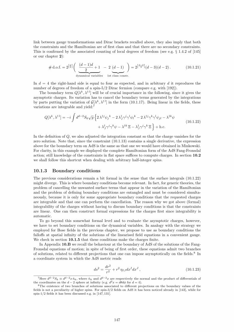
link between gauge transformations and Dirac brackets recalled above, they also imply that boththe constraints and the Hamiltonian are of first class and that there are no secondary constraints.This is confirmed by the associated counting of local degrees of freedom (see e.g. § 1.4.2 of [145]or our chapter 2):

# d.o.f. = 2[ d2 ](

(d− 1)d

2+ 1︸ ︷︷ ︸

dynamical variables

− 2 (d− 1)︸ ︷︷ ︸1st class constr.

)= 2[ d−2

2 ](d− 3)(d− 2) . (10.1.21)

In d = 4 the right-hand side is equal to four as expected, and in arbitrary d it reproduces thenumber of degrees of freedom of a spin-5/2 Dirac fermion (compare e.g. with [192]).

The boundary term Q[λk, λ† l] will be of crucial importance in the following, since it gives theasymptotic charges. Its variation has to cancel the boundary terms generated by the integrationsby parts putting the variation of G[λk, λ† l] in the form (10.1.17). Being linear in the fields, thesevariations are integrable and yield:7

Q[λk, λ† l] = −i∫dd−2Sk

√g

2λ†jψjk − 2λ†jγ

jγlψlk − 2λ†jγkγlψjl − λ†kψ

+ λ†jγjγkψ − λ†k Ξ− λ†jγjγk Ξ

+ h.c.

(10.1.22)

In the definition of Q, we also adjusted the integration constant so that the charge vanishes for thezero solution. Note that, since the constraint (10.1.13) contains a single derivative, the expressionabove for the boundary term on AdS is the same as that one we would have obtained in Minkowski.For clarity, in this example we displayed the complete Hamiltonian form of the AdS Fang-Fronsdalaction; still knowledge of the constraints in flat space suffices to compute charges. In section 10.2we shall follow this shortcut when dealing with arbitrary half-integer spins.

10.1.3 Boundary conditions

The previous considerations remain a bit formal in the sense that the surface integrals (10.1.22)might diverge. This is where boundary conditions become relevant. In fact, for generic theories, theproblem of cancelling the unwanted surface terms that appear in the variation of the Hamiltonianand the problem of defining boundary conditions are entangled and must be considered simulta-neously, because it is only for some appropriate boundary conditions that the requested chargesare integrable and that one can perform the cancellation. The reason why we got above (formal)integrability of the charges without having to discuss boundary conditions is that the constraintsare linear. One can then construct formal expressions for the charges first since integrability isautomatic.

To go beyond this somewhat formal level and to evaluate the asymptotic charges, however,we have to set boundary conditions on the dynamical variables. In analogy with the strategy weemployed for Bose fields in the previous chapter, we propose to use as boundary conditions thefalloffs at spatial infinity of the solutions of the linearised field equations in a convenient gauge.We check in section 10.1.5 that these conditions make the charges finite.

In Appendix 10.B we recall the behaviour at the boundary of AdS of the solutions of the Fang-Fronsdal equations of motion; in spite of being of first order, these equations admit two branchesof solutions, related to different projections that one can impose asymptotically on the fields.8 Ina coordinate system in which the AdS metric reads

ds2 =dr2

r2+ r2 ηIJdx

IdxJ , (10.1.23)

7Here dd−2Sk ≡ dd−2x nk, where nk and dd−2x are respectively the normal and the product of differentials ofthe coordinates on the d− 2 sphere at infinity (e.g. d2x = dθdφ for d = 4).

8The existence of two branches of solutions associated to different projections on the boundary values of thefields is not a peculiarity of higher spins. For spin-3/2 fields on AdS it has been noticed already in [143], while forspin-1/2 fields it has been discussed e.g. in [147,131].

147

the solutions in the subleading branch behave at spatial infinity (r →∞) as

ψIJ = r52−dQIJ(xK) +O(r

32−d) , (10.1.24a)

ψrI = O(r−d−12 ) , (10.1.24b)

ψrr = O(r−d−72 ) . (10.1.24c)

We remark that capital Latin indices denote all directions which are transverse to the radial one(including time) and that here and in the following we set the AdS radius to L = 1. The fieldequations further impose that QIJ satisfies the following conditions:

∂JQIJ = γJQIJ = 0 , (10.1.25a)

(1 + γr)QIJ = 0 , (10.1.25b)

where a hat indicates “flat” γ matrices, that do not depend on the point where the expressions areevaluated. For instance, γr = δrAγ

A. Eqs. (10.1.24) and (10.1.25) define our boundary conditions.In the case of spin 3/2 included in the discussion of section 10.2.2, the boundary conditions

dictated by the subleading solution of the linearised e.o.m. agree with those considered for N = 1AdS supergravity in four dimensions [143].9 This theory is known in closed form, and finiteness ofthe charges and consistency have been completely checked. Moreover, the agreement in the spin-3/2 sector extends a similar matching between the subleading falloffs of linearised solutions andthe boundary conditions generally considered in literature for gravity (see the previous chapter).These are our main motivations to adopt the boundary conditions defined by subleading linearisedsolutions for arbitrary values of the spin. See also section 10.1.6, where we show how the conditionsabove allow one to match results previously obtained in the Chern-Simons formulation of three-dimensional higher-spin gauge theories [73,136,128,210,78,66].

Since the action is of first order, the constraints (10.1.13) only depend on the dynamical vari-ables ψij and Ξ, that somehow play both the role of coordinates and momenta. The boundaryconditions (10.1.24) and (10.1.25), obtained from the covariant field equations, can therefore beeasily converted in boundary conditions on the canonical variables:

ψαβ = r52−dQαβ +O(r

32−d) , Ξ = − r 1

2−dQ00 +O(r−d−12 ) , (10.1.26a)

ψrα = O(r−d−12 ) , ψrr = O(r−d−

72 ) . (10.1.26b)

In the formulae above we displayed explicitly only the terms which contribute to the charges(see section 10.1.5) and we used Greek letters from the beginning of the alphabet to indicatethe coordinates that parameterise the d − 2 sphere at infinity. Furthermore, we used the γ-traceconstraint (10.1.25a) to fix the boundary value of Ξ.

10.1.4 Asymptotic symmetries

In order to specify the deformation parameters that enter the charge (10.1.22), we now identifyall gauge transformations preserving the boundary conditions of section 10.1.3. We begin byselecting covariant gauge transformations compatible with the fall-off conditions (10.1.24), andthen we translate the result in the canonical language.

Asymptotic symmetries contain at least gauge transformations leaving the vacuum solutionψµν = 0 invariant. These are generated by γ-traceless Killing spinor-tensors of the AdS background,which satisfy the conditions

D(µεν) +1

2γ(µεν) = 0 , γµεµ = 0 , (10.1.27)

and generalise the Killing spinors that are considered in supergravity theories (see [171] for adiscussion of the Killing spinors of AdSd along the lines we shall follow for higher spins). Weare not aware of any classification of γ-traceless Killing spinor-tensors of AdS spaces of arbitrary

9This is actually true up to a partial gauge fixing allowing one to match the falloffs of the radial component. Werefer to section 10.2.2 for more details.

148

dimension, but they have been discussed for d = 4 [67] and they are expected to be in one-to-onecorrespondence with the generators of the higher-spin superalgebras classified in [221]. In section10.C we shall also show that the number of independent solutions of (10.1.27) is the same as thatof its flat limit, whose general solution is given by (10.C.7). These arguments indicate that – asfar as the free theory is concerned – non-trivial asymptotic symmetries exist in any space-timedimension and we are going to classify them from scratch in the current spin-5/2 example. Alongthe way we shall observe that, when d > 3, asymptotic and exact Killing spinor-tensors only differin terms that do not contribute to surface charges.

To identify the gauge transformations that preserve the boundary conditions (10.1.24), one hasto analyse separately the variations of components with different numbers of radial indices. In thecoordinates (10.1.23), if one fixes the local frame as

erA = −1

rδrA , eI

J = ωIrJ = r δI

J , ωµνr = ωIJK = 0 , (10.1.28)

one obtains the conditions

δψIJ = 2(∂(IεJ) +

r

2γ(I| (1− γr) ε|J)

)+ 2 r3 ηIJεr = O(r

52−d) , (10.1.29)

δψrI =1

r

(r∂r −

4 + γr2

)εI +

(∂I +

r

2γI (1− γr)

)εr = O(r−d−

12 ) , (10.1.30)

δψrr =2

r

(r∂r +

2− γr2

)εr = O(r−d−

72 ) . (10.1.31)

Fronsdal’s γ-trace constraint /ε = 0 implies instead

γrεr = r−2 γIεI , (10.1.32)

thus showing that the radial component of the gauge parameter, εr, is not independent. It isanyway convenient to start analysing the conditions above from (10.1.31), which is a homogeneousequation solved by

εr = r−12 λ+(xk) + r−

32 λ−(xk) +O(r−d−

52 ) , with γrλ± = ±λ± . (10.1.33)

Substituting in (10.1.30) one obtains

εI = r52 ζ+

I + r32 ζ−I +

r12

2

(∂Iλ

+ + γIλ−)+

r−12

2∂Iλ− +O(r

12−d) , (10.1.34)

where the new boundary spinor-vectors that specify the solution satisfy

γrζ±I = ± ζ±I . (10.1.35)

The gauge parameter is further constrained by (10.1.29) and (10.1.32). The latter equationimplies

/ζ+ ≡ γIζ+

I = 0 , λ+ = /ζ−, (10.1.36)

and the differential conditions

/∂λ+ = −(d+ 1)λ− , /∂λ− = 0 . (10.1.37)

As shown in Appendix 10.C.3, the relations (10.1.37) are however not independent from theconstraints imposed by (10.1.29), so that we can ignore them for the time being. We stress thatin the equations above and in the rest of this subsection, contractions and slashed symbols onlyinvolve sums over transverse indices and flat γ matrices, so that /∂λ± = γI∂Iλ

±. Eq. (10.1.29)implies instead

δψIJ = 2 r52

(∂(IζJ)

+ + γ(IζJ)− + ηIJλ

+)

+ 2 r32

(∂(IζJ)

− + ηIJλ−)

+ r12

(∂I∂Jλ

+ + 2 γ(I∂J)λ−)+ r−

12 ∂I∂Jλ

− = O(r52−d) .

(10.1.38)

149

The cancellation of the two leading orders requires

λ+ = − 1

d− 1

(∂ · ζ+ + /ζ

−)

= −1

d∂ · ζ+ , λ− = − 1

d− 1∂ · ζ− , (10.1.39)

plus the differential conditions presented below in (10.1.41). In Appendix 10.C.3 we prove thatthese constraints also force the cancellation of the second line in (10.1.38) when d > 3. At theend of this subsection we shall instead comment on how to interpret the additional terms that oneencounters when d = 3.

To summarise: parameterising the AdSd background as in (10.1.23) and fixing the local frameas in (10.1.28), linearised covariant gauge transformations preserving the boundary conditions(10.1.24) are generated by

εI = r12 ζ+I + r−

12 ζ−I − r−

32

2d

(∂I∂ · ζ+ +

d

d− 1γI∂ · ζ−

)− r−

52

2(d− 1)∂I∂ · ζ−

+O(r−32−d) , (10.1.40a)

εr = −r32

d∂ · ζ+ − r

12

d− 1∂ · ζ− +O(r−d−

12 ) , (10.1.40b)

where the spinor-vectors ζ±I are subjected the chirality projections (10.1.35) and satisfy10

∂(IζJ)+ − 1

d− 1ηIJ ∂ · ζ+ = − γ(IζJ)

− +1

d− 1ηIJ γ · ζ− , (10.1.41a)

∂(IζJ)− − 1

d− 1ηIJ ∂ · ζ− = 0 , (10.1.41b)

γ · ζ+ = 0 , (10.1.41c)

γ · ζ− = −1

d∂ · ζ+ . (10.1.41d)

The left-hand sides of (10.1.41a) and (10.1.41b) have the same structure as the bosonic conformalKilling-vector equation in d−1 space-time dimensions. For this reason we call here the solutions of

(10.1.41) “conformal Killing spinor-vectors”. When d > 3 there are 2[ d−12 ](d− 2)(d+ 1) indepen-

dent solutions that we display in Appendix 10.C, while when d = 3 the space of solutions actuallybecomes infinite dimensional (see section 10.1.6).

As discussed in section 10.1.2, Fang-Fronsdal’s gauge parameters coincide with the deforma-tion parameters entering the charge (10.1.22). Asymptotic symmetries are therefore generated bydeformation parameters behaving as

λα = r12 ζ+α +O(r−

12 ) , λr = O(r

32 ) . (10.1.42)

As in (10.1.26), Greek letters from the beginning of the alphabet denote coordinates on the d− 2sphere at infinity and we specified only the terms that contribute to surface charges.

To conclude this subsection, we remark that an infinite number of solutions is not the uniquepeculiarity of the three-dimensional setup: in this case one indeed obtains

δψIJ = −r− 1

2

2∂I∂J∂ · ζ− +O(r−

32 ) (10.1.43)

even considering gauge parameters that satisfy (10.1.40) and (10.1.41). One can deal with thisvariation in two ways: if one wants to solve the Killing equation (10.1.27), one has to impose thecancellation of ∂I∂J∂ · ζ− and the additional condition is satisfied only on a finite dimensionalsubspace of the solutions of (10.1.41). If one is instead interested only in preserving the boundaryconditions (10.1.26), which is the only option when the background is not exact AdS space, a shift

of ψIJ at O(r−12 ) is allowed. In analogy with what happens for Bose fields [63] (see the previous

chapter), the corresponding variation of the surface charges is at the origin of the central chargethat appears in the algebra of asymptotic symmetries. In d = 3 the spinor-vector ζ−I enteringthe variation (10.1.43) indeed depends on the spinor-vector ζ+I entering the charges (see section10.1.6).

10These conditions also allow (10.1.40) to satisfy the γ-trace constraint (10.1.32), which is not manifest in theparameterisation of the solution we have chosen.

150

10.1.5 Charges

Having proposed boundary conditions on both canonical variables (see (10.1.26)) and deforma-tion parameters (see (10.1.42)), we can finally obtain the asymptotic charges. In the coordinates(10.1.23), the normal to the d − 2 sphere at infinity is such that nr = 1 and nα = 0. At theboundary the charge (10.1.22) thus simplifies as

limr→∞

Q[λk, λ† l] = i

∫dd−2x

√g

2λ†αγrγβψαβ − λ†αγαγr (ψ − Ξ)

+ h.c. (10.1.44)

The terms which survive in the limit give a finite contribution to the charge; one can make thismanifest by substituting their boundary values (where we drop the label + on ζ+I to avoid confu-sion) so as to obtain

Q = 2i

∫dd−2x

ζIQ0I + Q0I ζ

I. (10.1.45)

This presentation of Q relies on the γ-trace constraints on both QIJ and ζI and on the chiralityconditions (1 + γr)QIJ = 0 and (1 − γr)ζI = 0. Remarkably, the result partly covariantises inthe indices transverse to the radial direction. The boundary charge thus obtained is manifestlyconserved: it is the spatial integral of the time component of a conserved current since

JI ≡ 2i QIJζJ + h.c. ⇒ ∂ · J = 2i(∂IQIJζJ + QIJ∂(IζJ)

)+ h.c. = 0 , (10.1.46)

where conservation holds thanks to (10.1.25a) and (10.1.41a). Eq. (10.1.45) naturally extendsthe standard presentation of the bosonic global charges of the boundary theories entering thehigher-spin realisations of the AdS/CFT correspondence (see e.g. sect. 2.5 of [64]).

10.1.6 Three space-time dimensions

We conclude our analysis of the spin-5/2 example by evaluating the charge (10.1.45) in threespace-time dimensions, where several peculiarities emerge and we can compare our findings withthe results obtained in the Chern-Simons formulation of supergravity [13, 137] and higher-spintheories [73,136,128,210,78,66].

To proceed, it is convenient to introduce the light-cone coordinates x± = t±φ on the boundary.Two inequivalent representations of the Clifford algebra, characterised by γ0γ1 = ±γ2, are availablein d = 3. Since we conventionally fixed e.g. the relative sign in the gauge variation (10.1.2), weshall analyse them separately by choosing

γ± =

(0 20 0

), γ∓ =

(0 0−2 0

), γr =

(1 00 −1

). (10.1.47)

Equivalently, one could fix the representation of the Clifford algebra once for all and analyse theeffects of a simultaneous sign flip in the gauge variation (10.1.2) and in the chirality projections(10.1.25b) and (10.1.35).

One can exhibit the peculiar form of surface charges in d = 3 by studying the general solutionsof the conditions (10.1.25) and (10.1.41) on QIJ and ζI . The constraints on QIJ are solved by

Q∓∓ =

(0

Q(x∓)

), Q+− = Q±± =

(00

), (10.1.48)

where the signs are selected according to the conventions in (10.1.47). Note that the divergenceconstraint is satisfied by suitable left or right-moving functions as for bosons, but the interplaybetween the γ-trace constraint (10.1.25a) and the chirality projection (10.1.25b) forces one of thetwo chiral functions to vanish. Similarly, the constraints on ζ±I are solved by

ζ(+)∓ =

(ζ(x∓)

0

), ζ(−)∓ =

1

3

(0

∂∓ζ(x∓)

), ζ(+)± = ζ(−)± =

(00

), (10.1.49)

where we enclosed between parentheses the label denoting the chirality, which appears in thecovariant ζ±I of section 10.1.4.

151

When considering the representation of the Clifford algebra with γ0γ1 = ±γ2, the charge(10.1.45) therefore takes the form

Qd=3 = 2i

∫dφ ζ∗(x∓)Q(x∓) + c.c. , (10.1.50)

so that a single Fang-Fronsdal field is associated to infinitely many asymptotic conserved charges,corresponding to the modes of an arbitrary function which is either left or right-moving. Onthe contrary, a bosonic Fronsdal field is associated to both left and right-moving charges [63,64]. From the Chern-Simons perspective, the counterpart of this observation is the option todefine supergravity theories with different numbers of left and right supersymmetries [3]. Onecan similarly define higher-spin gauge theories in AdS3 by considering the difference of two Chern-Simons actions based on different supergroups (modulo some constraints on the bosonic subalgebra– see e.g. sect. 2.1 of [61]), while models with identical left and right sectors are associated to aneven numbers of Fang-Fronsdal fields.

10.2 Arbitrary spin

We are now going to generalise the results of the previous section to a spin s + 1/2 Dirac field,omitting the details that are not necessary to compute surface charges. As discussed at the end ofsection 10.1.2, these can be directly computed from the flat-space Hamiltonian constraints (whichdiffer from the AdSd ones through algebraic terms) and the boundary conditions of fields and gaugeparameters. We will focus on these two elements.

10.2.1 Constraints and gauge transformations

Our starting point is again the Fang-Fronsdal action for a massless spin s + 1/2 Dirac field onAdSd [104]:

S = −i∫ddx√−g

1

2ψ /Dψ +

s

2/ψ /D/ψ − 1

4

(s

2

)ψ′ /Dψ′ +

(s

2

)ψ′D · /ψ − s ψD/ψ

+d+ 2(s− 2)

4L

(ψψ − s /ψ/ψ − 1

2

(s

2

)ψ′ψ′

)+ h.c.

(10.2.1)

The conventions are the same as in the spin-5/2 example (we will use the same static parametri-sation of AdSd, etc., from section 10.1), except that we will now leave all indices (tensorial andspinorial) implicit. The field is a complex-valued spinor-tensor ψαµ1···µs

= ψα(µ1···µs), which is fullysymmetric in its s base-manifold indices µ1, . . . , µs. It will generally be denoted by ψ and itssuccessive traces will be indicated by primes or by an exponent in brackets: ψ[k] is the kth trace,while we often use ψ′ to denote a single trace.

The novelty of the general case is that there is an algebraic constraint on the field in addition tothat on the gauge parameter: its triple γ-trace is required to vanish, /ψ′ = 0. The only algebraicallyindependent components of the field have therefore zero, one or two tensorial indices in the timedirection: ψk1···ks , ψ0k2···ks and ψ00k3···ks .

The action (10.2.1) is invariant under gauge transformations

δψ = s

(Dε+

1

2Lγ ε

)(10.2.2)

generated by a γ-traceless spinor-tensor of rank s−1. In (10.2.2) and in the following, a symmetri-sation of all free indices is implicit, and dividing by the number of terms in the sum is understood.

Similarly to the spin-5/2 analysis, we note that the action (10.2.1) is almost already in canonicalform. To identify the Lagrange multipliers which enforce the first-class constraints associated tothe gauge symmetry (10.2.2), one can again select combinations whose gauge variation containstime derivatives of the gauge parameter. This leads to identify the dynamical variables with thespatial components ψk1...ks of the covariant field and with the combination

Ξk1···ks−2= f−2ψ00k1···ks−2

− 2 γ0γjψ0jk1···ks−2. (10.2.3)

152

The remaining independent components of the covariant fields, ψ0k1···ks−1 ≡ Nk1···ks−1 , play insteadthe role of Lagrange multipliers. The covariant gauge variation (10.2.2) breaks indeed into (withall contractions and omitted free indices being from now on purely spatial):

δψ = s

(∇ε+

1

2Lγε

), (10.2.4a)

δΞ = − 2 /∇/ε − (s− 2)∇ε′ + 1

2L[ 2 (d+ 1 + 2 (s− 2)) /ε − (s− 2) γε′ ] , (10.2.4b)

δN = ε+ f2γ0

[(s− 1)∇/ε −

1

2/Γε− (s− 1) Γ /ε −

1

2L(ε+ (s− 1) γ/ε)

]. (10.2.4c)

This choice of variables is further confirmed by injecting it back into the action (10.2.1), and usingthe Fronsdal constraint that sets the triple γ-trace of the field to zero, which leads to the followingidentities

ψ0···0k2n+1···ks = f2n[nΞ

[n−1]k2n+1···ks + 2nγ0 /N

[n−1]k2n+1···ks − (n− 1)ψ

[n]k2n+1···ks

], (10.2.5a)

ψ0···0k2n+2···ks = f2n[nγ0/Ξ

[n−1]k2n+2···ks + (2n+ 1)N

[n]k2n+2···ks − nγ

0/ψ[n]k2n+2···ks

]. (10.2.5b)

This brings the action into the canonical form

S =

∫ddx

1

2

(Ψ†A ω

ABΨB − Ψ†A ωABΨB

)−N†F [Ψ]−F†[Ψ†]N −H[Ψ,Ψ†]

, (10.2.6)

where we collected the phase-space variables by defining

ΨA =

(ψk1...ksΞk3...ks

), ωAB =

(ωk1···ks|l1···ls ωk1···ks|• i3···is

ω•j3...js|l1...ls ω•j3...js|• i3...is

). (10.2.7)

We will not exhibit all terms (symplectic 2-form, Hamiltonian, etc.) of this action, but only thosewhich are necessary to compute surface charges, that is the constraints. These have s− 1 implicitspatial indices symmetrised with weight one and read

F = −i√g

2

[s/2]∑n=0

(s

2n

)2nγ gn−1

[/∇Ξ[n−1] + (s− 2n)∇/Ξ[n−1]

+ 2 (n− 1)∇· /Ξ[n−2]

− /∇ψ[n] + (s− 2n)∇/ψ[n]+ 2n∇ · /ψ[n−1]

]+ (s− 2n) gn

[2n∇· Ξ[n−1]

+ (s− 2n− 1)∇Ξ[n] + 2 (n− 1)∇· ψ[n] + (s− 2n− 1)∇ψ[n+1] + 2 /∇/ψ[n]]

+ · · ·

(10.2.8)

The dots stand for algebraic contributions coming from the mass term in the action and possiblecontributions in Γi, which do not contribute to the surface charge.

Through their Dirac brackets (built from the inverse of the symplectic 2-form), these constraintsgenerate the gauge transformations (10.2.4a) and (10.2.4b), under which the Hamiltonian and theconstraints are invariant (which confirms that they are first class). The canonical generator ofgauge transformations is again

G[λ, λ†] =

∫dd−1x

(λ†F + F†λ

)+Q[λ, λ†] , (10.2.9)

where Q is the boundary term one has to add in order that G admits well defined functionalderivatives, i.e. that its variation be again a bulk integral:

δG =

∫dd−1x

(δψ†A+ δΞ†B +A†δψ +B†δΞ

). (10.2.10)

To compute surface charges we are only interested in Q (whose expression is independent ofthe terms we omitted in the constraint (10.2.8)). Its variation has to cancel the boundary termsgenerated by the integrations by parts putting the variation of G in the form (10.2.10). Being linear

153

in the fields, these variations are integrable and yield (we display explicitly the index k contractedwith dd−2Sk.):

Q[λ, λ†] =i

2

∫dd−2Sk

√g

[s/2]∑n=0

(s

2n

)2n[/λ†[n−1]

γk(

Ξ[n−1] − ψ[n])

+ (s− 2n) /λ†[n−1]k

(/ψ

[n]+ /Ξ

[n−1])

+ 2 (n− 1) /λ†[n−1]

/Ξ[n−2]k

+ 2n /λ†[n−1]

/ψ[n−1]k

]+ (s− 2n)

[(s− 2n− 1)λ†[n]k

(Ξ[n] + ψ[n+1]

)+ 2nλ†[n]Ξ[n−1]k

+ 2 (n− 1)λ†[n]ψ[n]k + 2λ†[n]γk /ψ[n]]

+ h.c.

(10.2.11)

In the definition of Q, we again adjusted the integration constant so that the charge vanishes forthe zero solution.

10.2.2 Boundary conditions and asymptotic symmetries

As in the spin-5/2 example, we derive boundary conditions on the dynamical variables from thefalloff at spatial infinity of the solutions of the Fang-Fronsdal equations in a convenient gauge,adopting the subleading branch. As shown in Appendix 10.B, with the parameterisation (10.1.4)of the local frame the relevant solutions behave at spatial infinity (r →∞) as

ψI1···Is = r52−dQI1···Is(xM ) +O(r

32−d) , (10.2.12a)

ψr···rI1···Is−n= O(r

52−d−3n) , (10.2.12b)

where capital Latin indices denote directions transverse to the radial one as in section 10.1.3.From now on we also set again L = 1. The boundary spinor-tensor QI1···Is is fully symmetric asthe Fang-Fronsdal field and satisfies

∂ · Q = /Q = 0 , (10.2.13a)

(1 + γr)Q = 0 , (10.2.13b)

where we omitted free transverse indices. Eqs. (10.2.12) and (10.2.13) define our boundary condi-tions. For s = 1 and d = 4 the requirements on ψI agree with those proposed for non-linear N = 1supergravity in eq. (V.1) of [143]. Our ψr decays instead faster at infinity, but the leading termthat we miss in (10.2.12b) can be eliminated using the residual gauge freedom parameterised bythe function a(t, θ, φ) in eq. (V.5) of [143]. In conclusion, on a gravitino our boundary conditionsagree with those considered in non-linear supergravity up to a partial gauge fixing that does notaffect the charges.

The covariant boundary conditions (10.2.12) fix the behaviour at spatial infinity of the dynam-ical variables as

ψα1···αs= r

52−dQα1···αs

+O(r32−d) , (10.2.14a)

ψr···rα1···αs−n = O(r52−d−3n) , (10.2.14b)

Ξα1···αs−2= − r 1

2−dQ00α1···αs−2+O(r−d−

12 ) , (10.2.14c)

Ξr···rα1···αs−n−2= O(r

12−d−3n) , (10.2.14d)

where Greek indices from the beginning of the alphabet denote angular coordinates in the d − 2sphere at infinity. Moreover, we displayed only the dependence on the boundary values of the fieldsin the terms that actually contribute to surface charges.

The next step in the procedure we illustrated in section 10.1 requires to identify all gaugetransformations that do not spoil the boundary conditions (10.2.14). We are now going to providenecessary conditions for the preservation of the asymptotic form of the fields, which generalise thosegiven for s = 2 in (10.1.40) and (10.1.41). A proof that they are also sufficient (along the lines of theproof presented for s = 2 in Appendix 10.C.3) will be given elsewhere. We stress, however, that

154

the rank-s counterparts of (10.1.40) and (10.1.41) also characterise the exact γ-traceless Killingspinor-tensors of AdSd, which satisfy

Dε+1

2γ ε = 0 , /ε = 0 . (10.2.15)

The general solution of these equations is provided in Appendix 10.C for s = 2. It shows that thenumber of independent solutions is the same as in the flat-space limit, where Killing spinor-tensorsare easily obtained (see (10.C.9)). In the following we assume that this concurrence holds forarbitrary values of the spin and, hence, that the conditions we are going to present admit as manyindependent solutions as integration constants in (10.C.9).

To characterise the gauge parameters which generate asymptotic symmetries, one has to analyseseparately the variations of components with different numbers of radial indices. We continue toomit transverse indices and we denote them as

ψn ≡ ψr···rI1···Is−n. (10.2.16)

Similarly, we denote by εn the component of the gauge parameter with n radial indices. With thechoice (10.1.4) for the local frame, the variations of the field components must satisfy

δψn =n

r

(r∂r −

2(2s− 3n+ 1) + γr

2

)εn−1 + (s− n)

(∂ +

r

2γ (1− γr)

)εn

+ 2

(s− n

2

)r3η εn+1 = O(r

52−d−3n) .

(10.2.17)

The constraint /ψ′ = 0 actually implies that one can focus only on the variations of ψ0, ψ1 and ψ2,since all other components are not independent. One also has to consider the constraint /ε = 0,which implies

γrεn+1 = r−2/εn (10.2.18)

and shows that the only independent component of the gauge parameter is the purely transverseone, that is ε0 ≡ εI1···Is−1

.The equations (10.2.17) require11

ε0 = r2(s−1)(r

12 ζ+ + r−

12 ζ−

)+

s−1∑k=1

r2(s−k−1)(r

12αk + r−

12 βk

)+O(r

12−d) (10.2.19)

together with the chirality projections

(1∓ γr)ζ± = 0 (10.2.20)

and similar restrictions on the subleading components: (1− γr)αk = (1 + γr)βk = 0. The γ-traceconstraint on the gauge parameter is then satisfied by

ε2n = (−1)ns−n−1∑k=n

r2(s−2n−k−1)(r

12α

[n]k + r−

12 β

[n]k

)+O(r

12−d−6n) , (10.2.21a)

ε2n+1 = (−1)ns−n−2∑k=n

r2(s−2n−k)−5(r

12 /β

[n]k − r

− 12 /α

[n]k

)+O(r−d−

52−6n) . (10.2.21b)

11This can be shown e.g. by considering the redundant variation of ψs ≡ ψr···r, which gives a homogeneousequation for εs−1 ≡ εr···r as in section 10.1.4. One can then fix recursively the r-dependence of all other componentsof the gauge parameter.

155

Substituting these expressions in (10.2.17) one obtains

δψ0 = s r2(s−1)r

12

[∂ζ+ + γζ− + (s− 1) η /ζ

−]

+ r−12

[∂ζ− − (s− 1) η /α1

]+ s

s−1∑k=1

r2(s−k−1)r

12 [∂αk + γβk + (s− 1) η /βk] + r−

12

[∂βk − (s− 1) η /αk+1

], (10.2.22a)

δψ1 =

s−1∑k=1

r2(s−k)−3r

12 [−2k αk + (s− 1) (∂/βk−1 − γ/αk)− (s− 1)(s− 2) η α′k]

+ r−12

[−2k βk − (s− 1)

(∂/αk + (s− 2)η β ′k

)]. (10.2.22b)

In complete analogy with the analysis of section 10.1.4, the cancellation of the first line in(10.2.22a) requires

∂ζ+ − s− 1

d+ 2s− 4η ∂ · ζ+ + γ ζ− = 0 , (10.2.23a)

∂ζ− − s− 1

d+ 2s− 5η ∂ · ζ− = 0 , (10.2.23b)

γ · ζ+ = 0 , (10.2.23c)

γ · ζ− +1

d+ 2s− 4∂ · ζ+ = 0 . (10.2.23d)

These conditions generalise the conformal Killing equations (10.1.41) to arbitrary values of therank. Their general solution is given below in (10.2.28) when d = 3, while for d > 3 it will be givenelsewhere. Still, as anticipated, the detailed analysis of the s = 2 case presented in Appendix 10.Cmakes us confident that the equations (10.2.23) admit a number of independent solutions equal tothe number of integration constants in (10.C.9).

The subleading orders in (10.2.22) allow instead to fix the subleading components of the gaugeparameter in terms of ζ±. For instance, one can manipulate these expressions to obtain therecursion relations presented in Appendix 10.C.3. Let us stress that, in analogy with what weobserved for s = 2, (10.2.22a) and (10.2.22b) provide a set of equations that are compatible only ifone takes into account the constraints (10.2.23). We do not have yet a proof of the latter statement,but the analysis given for s = 2 in Appendix 10.C gives strong indications that this is a robustassumption.

The deformation parameters that generate gauge transformations preserving the boundaryconditions can then be related to Fang-Fronsdal’s gauge parameters by comparing the Lagrangianfield equations with their rewriting in (2.3.15) and (2.3.18). In particular, the Dirac brackets withthe constraints can be inferred from the terms with Lagrange multipliers contained in the equationsexpressing the time derivatives of the dynamical variables in terms of the spatial derivatives of ψµν .This shows that the gauge parameter can be identified with the canonical deformation parameteralso for arbitrary values of the spin. As a result, the latter behaves at spatial infinity as

λα1···αs−1 = r12 ζ+α1···αs−1 +O(r−

12 ) , λr···rα1···αs−n−1 = O(r

12 +n) , (10.2.24)

where ζ+ satisfies the conformal Killing equations (10.2.23) and, as in (10.2.14), Greek indicesfrom the beginning of the alphabet denote angular coordinates in the d− 2 sphere at infinity.

10.2.3 Charges

Having proposed boundary conditions on both canonical variables (see (10.2.14)) and deformationparameters (see (10.2.24)), we can finally evaluate the asymptotic charges. The charge (10.2.11)simplifies at the boundary as

limr→∞

Q[λ, λ†] = i

∫dd−2x

√g

[s/2]∑n=0

(s

2n

)n /λ†[n−1]

γr(

Ξ[n−1] − ψ[n])

+ (s− 2n)λ†[n]γr /ψ[n]

+ h.c. ,

(10.2.25)

156

where all implicit indices are now purely spatial and transverse and we dropped the label + on ζ+

to avoid confusion.The terms which survive in the limit give a finite contribution to the charge; one can make this

manifest by substituting their boundary values so as to obtain

Q = s i

∫dd−2x

ζI2...IsQ0I2...Is + Q0I2...Is ζ

I2...Is, (10.2.26)

where we used the γ-trace constraints on both Q and ζ and the chirality conditions (1 + γr)Q = 0and (1− γr)ζ = 0. The result partly covariantises in the indices transverse to the radial directionas in the spin-5/2 example, thus making the conservation of the charge manifest. It is indeed thespatial integral of the current JI = ζK2...KsQIK2...Ks

+ h.c., which is conserved thanks to (10.2.13a)and (10.2.23).

In three space-time dimensions the charge (10.2.26) is actually given by a left or right-movingfunction also for arbitrary half-integer values of the spin. As in section 10.1.6, one can dealwith the two inequivalent representations of the Clifford algebra by choosing the γ matrices as in(10.1.47). The constraints on Q are then solved by

Q∓···∓ =

(0

Q(x∓)

), Q±···± = Q+···+−···− =

(00

), (10.2.27)

where different signs correspond to the choices γ0γ1 = ±γ2. Similarly, the conformal Killingequations (10.2.23) are solved by

ζ(+)∓···∓ =

(ζ(x∓)

0

), ζ(−)∓···∓ =

1

2s− 1

(0

∂∓ζ(x∓)

), (10.2.28a)

ζ(±)±···± = ζ(±)+···+−···− =

(00

), (10.2.28b)

where we enclosed again between parentheses the label denoting the chirality of the spinor-tensors.The charge (10.2.26) takes therefore the form

Qd=3 = s i

∫dφ ζ∗(x∓)Q(x∓) + c.c. , (10.2.29)

which generalises the result for the spin-5/2 case discussed in section 10.1.6.

10.3 Summary and further developments

We have explicitly constructed higher-spin charges for fermionic gauge fields of arbitrary spin onAdS backgrounds in any number of spacetime dimensions, extending our analogous work on bosonicgauge fields [64] (see the previous chapter). We have followed Hamiltonian methods. The chargesappear as the surface integrals that must be added to the terms proportional to the constraintsin order to make the generators of gauge transformations well-defined as phase-space generators.These integrals are finite with the boundary conditions that we have given, which crucially involvechirality-type projections generalising those of [143]. Improper gauge transformations – associatedto non-vanishing surface integrals – are determined by conformal Killing spinor-tensors of theboundary, and the corresponding charges take a simple, boundary-covariant expression in terms ofthem – even though the intermediate computations are sometimes rather involved. While bosonichigher-spin charges have been derived also following other approaches [15,225,91], to our knowledgeour treatment provides the first presentation of fermionic higher-spin charges that applies to anynumber of space-time dimensions

We confined our analysis to the linearised theory, which suffices to derive the charges. In thiscontext, however, the charges are abelian and their Dirac brackets vanish (modulo possible centralextensions in d = 3). To uncover a non abelian algebra, one must evaluate the brackets in thenon-linear theory, since the bulk terms do play a role in that computation. A similar situationoccurs for Yang-Mills gauge theories, where the surface terms giving the charges coincide withthose of the abelian theory. The non-abelian structure appears when one computes the algebra

157

of the charges, a step which involves the full theory (or, generically, at least the first non-linearcorrections in a weak field expansion [63]).

By working within the linearised theory, we have been able to associate conserved charges toany gauge field of given spin, although the spectra of interacting higher-spin theories are typicallyvery constrained. We also worked with Dirac fields, that can be defined for any d, but the Majoranaand/or Weyl projections that one may need to consistently switch on interactions can be easilyimplemented in our approach. In general, we have not found obstructions to define non-trivialhigher-spin charges in any number of space-time dimensions and for arbitrary multiplicities ofany value of the spin, consistently with the chance to define higher-spin algebras with fermionicgenerators in any dimension [67,221]. Possible constraints could emerge from interactions, but letus point out that once one starts considering half-integer higher spins, more exotic options thanstandard supersymmetry may become available. For instance, one can define higher-spin theorieswith increasing multiplicities for the fermionic fields without introducing any obvious pathology –apart from difficulties in identifying a superconformal subalgebra within their algebra of asymptoticsymmetries (see e.g. [67, 66]) – or try to define “hypersymmetric” theories (see e.g. [56]) – withfermionic gauge symmetries but without any gravitino at all. To analyse these phenomena itwill be very interesting to combine our current results with those obtained for Bose fields [64],and to analyse the effect of interactions on the algebra of surface charges, e.g. introducing themperturbatively in a weak field expansion (see [41, 166, 63] for related work restricted to bosonicmodels).

158

Appendix

10.A Notation and conventions

We adopt the mostly-plus signature for the space-time metric gµν and we often distinguish amongtime and spatial components by breaking space-time indices as µ = (0, i). Tangent-space indicesare collectively denoted by capital Latin letters, but when we separate time and spatial directionswe use the same letters as for the indices on the base manifold, i.e. A = (0, i). The γ matrices thensatisfy

γA, γB = ηAB , (γ0)† = − γ0 , (γi)† = γi , (10.A.1)

where the hat differentiates them from their curved counterparts involving the inverse vielbein:

γµ = eµA γA . (10.A.2)

For instance, with the choice (10.1.4) for the local frame one has γ0 = fγ0. Similarly, the Diracconjugate is defined as ψ = ψ†γ0, while the γ matrices displayed explicitly in the Fronsdal action(see e.g. (10.1.1) or (10.2.1)) are curved ones.

The space-time covariant derivative acts on a spin s+ 1/2 field as

Dρψµ1···µs = ∂ρψµ1···µs +1

8ωρ

AB [γA, γB ]ψµ1···µs− sΓλρ(µ1

ψµ2···µs)λ , (10.A.3)

and it satisfies Dµγν = 0. In the definition we omitted spinor indices as in the rest of the chapter.Moreover, indices between parentheses are meant to be symmetrised with weight one, i.e. onedivides the symmetrised expression by the number of terms that appears in it. The spatial covariantderivative ∇ is defined exactly as in (10.A.3), but with indices constrained to take values only alongspatial directions. It also satisfies ∇iγj = 0.

On an (A)dS background the commutator of two covariant derivatives reads

[Dµ, Dν ]ψρ1···ρs =s

L2

(gν(ρ1ψρ2···ρs)µ − gµ(ρ1ψρ2···ρs)ν

)− 1

2L2γµνψρ1···ρs , (10.A.4)

where γµν = 12 [γµ, γν ]. This relation defines the (A)dS radius L and suffices to fix the mass term

in the Fronsdal action (10.2.1).When expanding tensors in components, we actually distinguish among four types of indices,

depending on whether the time and/or radial coordinates are included or not. Greek letters fromthe middle of the alphabet include all coordinates, small Latin letters include all coordinates exceptt, capital Latin letters include all coordinates except r, while Greek letters from the beginning ofthe alphabet denote the angular coordinates on the unit d− 2 sphere. In summary:

µ, ν, . . . ∈ t, r, φ1, . . . , φd−2 , i, j, . . . ∈ r, φ1, . . . , φd−2 ,I, J, . . . ∈ t, φ1, . . . , φd−2 , α, β, . . . ∈ φ1, . . . , φd−2 . (10.A.5)

Slashed symbols always denote a contraction with a γ matrix, whose precise meaning dependson the context: the contraction may be with the full γµ or with its spatial counterpart γi. Insection 10.1 omitted indices denote a trace that, similarly, may result from a contraction with thefull space-time metric gµν or with the spatial metric gij . In most of section 10.2 we omit insteadall indices, which are always assumed to be fully symmetrised according to the conventions givenabove. Traces are instead denoted by an exponent between square brackets, so that, for instance,

ψ[n] ≡ ψµ1···µs−2nλ1···λn

λ1···λn , Dψ ≡ D(µ1ψµ2···µs+1) , γ ψ ≡ γ(µ1

ψµ2···µs+1) . (10.A.6)

159

In Appendix 10.B we reinstate indices with the following convention: repeated covariant or con-travariant indices denote a symmetrisation, while a couple of identical covariant and contravariantindices denotes as usual a contraction. Moreover, the indices carried by a tensor are substitutedby a single label with a subscript indicating their total number. For instance, the combinations in(10.A.6) may also be presented as

ψ[n] = ψµs−2n, Dψ = Dµψµs

, γ ψ ≡ γµψµs. (10.A.7)

160

10.B Covariant boundary conditions

In this appendix we recall the falloff at the boundary of AdSd of the solutions of the Fang-Fronsdalequations of motion (see also [181]). To achieve this goal we partially fix the gauge freedom, andwe also exhibit the falloffs of the parameters of the residual gauge symmetry (which include theγ-traceless Killing spinor-tensors of AdSd).

We set the AdS radius to L = 1 and we work in the Poincare patch parameterised as

ds2 =1

z2

(dz2 + ηIJdx

IdxJ). (10.B.1)

We also fix the local frame as

eµA =

1

zδµA , ωI

zJ =1

zδIJ , ωz

µν = ωIJK = 0 , (10.B.2)

where we take advantage of the form of the vielbein to identify “flat” and “curved” indices. Inthese coordinates the spatial boundary is at z → 0. All results can be easily translated in thecoordinates (10.1.3) used in the main body of the text, in which the boundary is at r → ∞. Wedenote by capital Latin indices all directions transverse to the radial one (including time).

10.B.1 Falloff of the solutions of the free equations of motion

We wish to study the solutions of the Fang-Fronsdal equation on a constant-curvature backgroundof dimension d [104] which, in the index-free notation of section 10.2, reads

i

(/Dψ − sD/ψ +

d+ 2(s− 2)

2ψ +

s

2γ /ψ

)= 0 . (10.B.3)

To this end it is convenient to partially fix the gauge freedom (10.2.2) by setting to zero the γ-traceof the field (see [79] or sect. 2.2 of the review [192] for a discussion of this partial gauge fixing inflat space). This leads to the system of equations

i

(/D +

d+ 2(s− 2)

2

)ψ = 0 , (10.B.4a)

/ψ = 0 . (10.B.4b)

These conditions also imply that the divergence of the field vanishes: taking the γ-trace of the firstequation one indeed obtains

0 = γµ /Dψµ = − /D/ψ + 2D · ψ , (10.B.5)

that implies D · ψ = 0 thanks to the second equation. Imposing (10.B.4b) does not fix completelythe gauge freedom: eqs. (10.B.4) admit a residual gauge symmetry with parameters constrainedas (

/D +d+ 2(s− 1)

2

)ε = 0 , (10.B.6a)

D · ε = 0 , (10.B.6b)

/ε = 0 , (10.B.6c)

where the cancellation of the divergence follows from the other two conditions as above.12

To analyse the falloff at z → 0 of the solutions of (10.B.4) one has to treat separately fieldcomponents with a different number of indices along the z direction. We denote them as

ψznIs−n ≡ ψz···zI1···Is−n . (10.B.7)

12Eqs. (10.B.6) manifestly guarantee that gauge transformations of the form (10.2.2) preserve the γ-trace con-straint (10.B.4b). The divergence constraint (10.B.5) is also preserved thanks to

δ D · ψ =

(+

1

2/D −

(s− 1)(2d+ 2s− 5)

2

)ε =

(/D −

d+ 2s− 3

2

)(/D +

d+ 2(s− 1)

2

)ε .

161

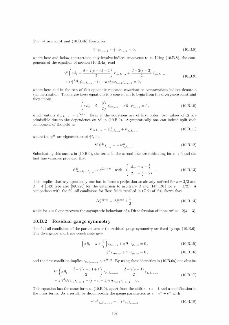
The γ-trace constraint (10.B.4b) then gives

γz ψzµs−1+ γ · ψµs−1

= 0 , (10.B.8)

where here and below contractions only involve indices transverse to z. Using (10.B.8), the com-ponents of the equation of motion (10.B.4a) read

γz(z ∂z −

d− 2(s− n)− 1

2

)ψznIs−n

+d+ 2(s− 2)

2ψznIs−n

+ z γJ∂JψznIs−n− (s− n) γIψzn+1Is−n−1

= 0 ,

(10.B.9)

where here and in the rest of this appendix repeated covariant or contravariant indices denote asymmetrisation. To analyse these equations it is convenient to begin from the divergence constraintthey imply, (

z ∂z − d+3

2

)ψzµs−1

+ z ∂ · ψµs−1= 0 , (10.B.10)

which entails ψznIs−n∼ z∆+n. Even if the equations are of first order, two values of ∆ are

admissible due to the dependence on γz in (10.B.9). Asymptotically one can indeed split eachcomponent of the field as

ψznIs−n = ψ+znIs−n

+ ψ−znIs−n, (10.B.11)

where the ψ± are eigenvectors of γz, i.e.

γzψ±znIs−n= ∓ψ±znIs−n

. (10.B.12)

Substituting this ansatz in (10.B.9), the terms in the second line are subleading for z → 0 and thefirst line vanishes provided that

ψ±z···z I1···Is−n∼ z∆±+n with

∆+ = d− 5

2

∆− = 32 − 2s

. (10.B.13)

This implies that asymptotically one has to force a projection as already noticed for s = 3/2 andd = 4 [143] (see also [69, 226] for the extension to arbitrary d and [147, 131] for s = 1/2). Acomparison with the fall-off conditions for Bose fields recalled in (C.9) of [64] shows that

∆Fermi± = ∆Bose

± ± 1

2, (10.B.14)

while for s = 0 one recovers the asymptotic behaviour of a Dirac fermion of mass m2 = −2(d− 3).

10.B.2 Residual gauge symmetry

The fall-off conditions of the parameters of the residual gauge symmetry are fixed by eqs. (10.B.6).The divergence and trace constraints give(

z ∂z − d+3

2

)εzµs−2 + z ∂ · εµs−2 = 0 , (10.B.15)

γz εzµs−2+ γ · εµs−2

= 0 , (10.B.16)

and the first condition implies εznjs−n−1 ∼ zΘ+n. By using these identities in (10.B.6a) one obtains

γz(z ∂z −

d− 2(s− n) + 1

2

)εznIs−n−1

+d+ 2(s− 1)

2εznIs−n−1

+ z γJ∂JεznIs−n−1 − (s− n− 1) γIεzn+1Is−n−2 = 0 .

(10.B.17)

This equation has the same form as (10.B.9), apart from the shift s→ s− 1 and a modification inthe mass terms. As a result, by decomposing the gauge parameters as ε = ε+ + ε− with

γzε±znIs−n−1= ∓ ε±znIs−n−1

(10.B.18)

162

and following the same steps as above one obtains

ε±z···z I1···Is−n−1∼ zΘ±+n with

Θ+ = d− 1

2

Θ− = 32 − 2s

. (10.B.19)

A comparison with the fall-off conditions in (C.12) of [64] shows that

ΘFermi± = ΘBose

± ± 1

2(10.B.20)

also for gauge parameters.One can compare these results with the conditions satisfied by a gauge transformation preserv-

ing the AdS background, for which

δψ = s

(Dε+

1

2γ ε

)= 0 , /ε = 0 . (10.B.21)

These constraints also imply D · ε = 0. Expanding (10.B.21) one obtains(z ∂z + (2s− n− 2) +

1

2γz)εznIs−n−1 = O(zΘ+n+1) . (10.B.22)

This equation is analysed more in detail in section 10.2.2; here it is worth noting that the solutionsin the Θ− branch of (10.B.19) also solve (10.B.22).

10.B.3 Initial data at the boundary

In this subsection we display the constraints on the initial data at the boundary imposed by theequations of motion and the γ-trace constraint, and how the number of independent componentsis further reduced by the residual gauge symmetry. First of all, note that the solutions of (10.B.4)are generically of the form

ψzmIs−m=

∞∑n=0

z∆++m+nq(m,n)Is−m

(xk) or ψzmIs−m=

∞∑n=0

z∆−+m+nρ(m,n)Is−m

(xk) , (10.B.23)

where all spinor-tensors in the series have a definite (alternating) chirality:13

γzq(m,n) = (−1)n+1q(m,n) , γzρ(m,n) = (−1)nρ(m,n) . (10.B.24)

The γ-trace constraint (10.B.8) then allows one to solve all components ψznIs−nwith n ≥ 1 in

terms of the purely transverse one, ψIs . The equation of motion (10.B.9) finally fixes the subleadingcomponents of ψIs in terms of the leading one.

Within the admissible fall-off conditions, the ∆+ branch is the one which is relevant for theanalysis of surface charges. We denote its leading contributions in ψIs as

ψIs = z∆+Q−Is(xK) + z∆++1Q+Is

(xK) +O(z∆++2) , (1∓ γz)Q±Is = 0 . (10.B.25)

For completeness, we shall also analyse the constraints imposed on the leading contributions in the∆− branch, denoted as

ψIs = z∆−Ψ+Is

(xK) + z∆−+1Ψ−Is(xJ) +O(z∆−+2) , (1∓ γz)Ψ±Is = 0 . (10.B.26)

The spinor-tensors Q−Is and Ψ+Is

are boundary fields of opposite chirality (or, when the dimensionof the boundary is odd, Dirac fields with different eigenvalues of γz) of conformal dimensions,respectively, ∆c = d + s − 5

2 and ∆s = 32 − s. They thus correspond to the fermionic conserved

currents and shadows fields of [181].14

13The components of e.g. the q(m,n)Is−n

can be considered as spinors defined on the (d− 1)-dimensional boundary of

AdS. When d is odd, (10.B.24) is a chirality projection. When d is even, a priori the boundary values of ψIJ wouldbe collected in a couple of Dirac spinors and (10.B.24) selects one of them.

14If one performs a dilatation xµ → λxµ then ψI′s = λ−sψIs , while on the right-hand side of (10.B.25) or (10.B.26)

one has z′∆± = λ∆±z∆± . As a result, both Q and Ψ must transform as QI′s = λ−(∆++s)QIs , from where one reads

the conformal dimensions. To compare them with eqs. (5.8) and (6.6) of [181], consider that dhere = (d+ 1)there.

163

Combining the e.o.m. (or, equivalently, the divergence constraint) and the γ-trace constraintgives

∂JQ−JIs−1= 0 , γJQ−JIs−1

= ηJKQ+JKIs−2

= 0 . (10.B.27)

Eq. (10.B.9) also allows one to fix the γ-traceless component of Q+ as(Q+Is

)Tr ≡ Q+Is− s

d+ 2s− 3γI /Q

+Is−1

= − 1

d+ 2s− 3/∂Q−Is . (10.B.28)

The γ-trace of Q+ remains free as the divergenceless part of Q−. In the ∆− branch the γ-traceconstraint similarly imposes

γJΨ+JIs−1

= ηJKΨ−JKIs−2= 0 . (10.B.29)

The full γ-traceless Ψ+ remains instead unconstrained, while all Ψ− is now fixed as

Ψ−Is = − 1

d+ 2s− 5

(/∂Ψ+

Is− s

d+ 2s− 4γI ∂ ·Ψ

+Is−1

). (10.B.30)

Note that, in analogy with Bose field [64], the total number of independent data that asymptoticallycan be chosen arbitrarily15 is the same in both branches, even if they are distributed in differentways in (10.B.25) and (10.B.26).

The number of independent initial data is further reduced by the residual gauge symmetry.The components of the field vary as

z δψznIs−n= n

(z ∂z + 2s− n− 1 +

γz

2

)εzn−1Is−n

+s− n

2γI(1− γz) εznIs−n−1

+ (s− n)(z ∂IεznIs−n−1

− (s− n− 1)ηIIεzn+1Is−n−2

).

(10.B.31)

Gauge transformations generated by

εznIs−n−1 = zΘ++n ξ(n)Is−n−1

(xK) +O(zΘ++n+1) , (1 + γz) ξ(n)Is−n−1

= 0 , (10.B.32)

naturally act on the ∆+ branch of solutions of the e.o.m.: they allow to set to zero the ψznIs−n

components with n ≥ 1 (and therefore also /Q+), while they leave Q− invariant. On the other

hand, gauge transformations generated by

εznIs−n−1 = zΘ−+n ε(n)Is−n−1

(xK) +O(zΘ−+n+1) , (1− γz) ε(n)Is−n−1

= 0 , (10.B.33)

naturally act on the ∆− branch and they affect the leading contribution as

δΨ+Is

= s ∂IεIs−1− s

d+ 2s− 3

(γI/∂εIs−1

+ (s− 1)ηII∂ · εIs−2

), (10.B.34)

where we defined ε ≡ ε(0) and the variation is γ-traceless as it should. This gauge freedom reducesthe number of independent components Ψ+ such that it becomes identical to that of the conservedcurrent Q−. It also leaves the coupling i

(Ψ+Q− + Q−Ψ+

)invariant.

15Of course, regularity in the bulk should fix the vev in terms of the source. We do not discuss this issue here aswe focus on the asymptotic behaviour of the theory. Integration in the bulk necessitates the full theory beyond thelinear terms.

164

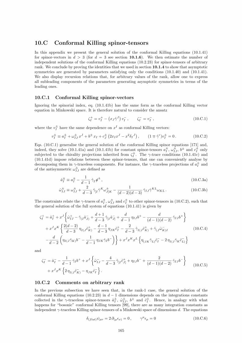
10.C Conformal Killing spinor-tensors

In this appendix we present the general solution of the conformal Killing equations (10.1.41)for spinor-vectors in d > 3 (for d = 3 see section 10.1.6). We then estimate the number ofindependent solutions of the conformal Killing equations (10.2.23) for spinor-tensors of arbitraryrank. We conclude by proving the identities that we used in section 10.1.4 to show that asymptoticsymmetries are generated by parameters satisfying only the conditions (10.1.40) and (10.1.41).We also display recursion relations that, for arbitrary values of the rank, allow one to expressall subleading components of the parameters generating asymptotic symmetries in terms of theleading ones.

10.C.1 Conformal Killing spinor-vectors

Ignoring the spinorial index, eq. (10.1.41b) has the same form as the conformal Killing vectorequation in Minkowski space. It is therefore natural to consider the ansatz

ζ+I = v+

I −(xJ γ

J)v−I , ζ−I = v−I , (10.C.1)

where the v±I have the same dependence on xI as conformal Killing vectors:

v±I ≡ a±I + ω±IJ x

J + b± xI + c±J(2xIx

J − x2δIJ), (1∓ γr)v±I = 0 . (10.C.2)

Eqs. (10.C.1) generalise the general solution of the conformal Killing spinor equations [171] and,indeed, they solve (10.1.41a) and (10.1.41b) for constant spinor-tensors a±I , ω±IJ , b± and c±I onlysubjected to the chirality projections inherited from ζ±I . The γ-trace conditions (10.1.41c) and(10.1.41d) impose relations between these spinor-tensors, that one can conveniently analyse bydecomposing them in γ-traceless components. For instance, the γ-traceless projections of a±I andof the antisymmetric ω±IJ are defined as

a±I ≡ a±I −

1

d− 1γI /a

± , (10.C.3a)

ω±IJ ≡ ω±IJ +

2

d− 3γ[I γ

Kω±J]K −1

(d− 2)(d− 3)γIJ γ

KLωKL . (10.C.3b)

The constraints relate the γ-traces of a±I , ω±IJ and c±I to other spinor-tensors in (10.C.2), such thatthe general solution of the full system of equations (10.1.41) is given by

ζ+I = a+

I + xJω+IJ − γ(I a

−J) +

d+ 1

d− 3γ[I a

−J] +

d

d− 1ηIJb

+ − d

(d− 1)(d− 2)γIJb

+

+ xJxK

2(d− 2)

d− 3ηI(J c

+K) −

d− 1

d− 3ηJK c

+I −

2

d− 3γI(J c

+K) + γ(J ω

−K)I

− d

d− 2

(ηI(J γK)b

− − 1

d− 1ηJK γIb

−)

+ xJxKxLη(JK γL)c

−I − 2 ηI(J γK c

−L)

(10.C.4)

and

ζ−I = a−I −1

d− 1γIb

+ + xJω−IJ −

4

d− 3γ[I c

+J] + ηIJb

− +2

(d− 1)(d− 2)γIJb

−

+ xJxK

2 ηI(J c−K) − ηJK c

−I

.

(10.C.5)

10.C.2 Comments on arbitrary rank

In the previous subsection we have seen that, in the rank-1 case, the general solution of theconformal Killing equations (10.2.23) in d − 1 dimensions depends on the integrations constantscollected in the γ-traceless spinor-tensors a±I , ω±IJ , b± and c±I . Hence, in analogy with whathappens for “bosonic” conformal Killing tensors [99], there are as many integration constants asindependent γ-traceless Killing spinor-tensors of a Minkowski space of dimensions d. The equations

δ(flat)ψµν = 2 ∂(µεν) = 0 , γµεµ = 0 (10.C.6)

165

are indeed solved by

εµ = Aµ +Bµνxν , γµAµ = γµBµν = B(µν) = 0 , (10.C.7)

and the number of independent components of the constants Aµ and Bµν in d dimensions equatesthat of a±I , ω±IJ , b± and c±I in d − 1 dimensions. This indicates that the number of independentγ-traceless Killing spinor-tensors on AdS and Minkowski backgrounds is the same (at least up torank 1).

The pattern of independent spinor-tensors entering (10.C.2) can be understood from the branch-ing rules for representations of the orthogonal group (see e.g. § 8.8.A of [20]). Denoting a Youngtableau with s boxes in the first row and k boxes in the second by s, k, a γ-traceless s, k-projected spinor-tensor in d+1 dimensions decomposes in a sum of two-row projected spinor-tensorsin d dimensions as16

s, kd =

s∑r=k

k∑l=0

n(d)r, ld−1 , (10.C.8)

where the multiplicity factor n(d) is equal to 1 when d is odd and to 2 when d is even. Applyingthis rule to Aµ and Bµν , one recovers the spinor-tensors entering (10.C.2). When d is odd, the± doubling in (10.C.2) allows to reproduce the components of a Dirac εµ from two sets of Weylspinor-tensors. When d is even, the doubling accounts for the factor n(d) in (10.C.8).

A full derivation of the solutions of the conformal Killing equations (10.2.23) will be givenelsewhere (see also [153] for related work based on superspace techniques). Here we assume that thepattern emerged in the rank 0 and 1 examples extends to arbitrary values of the rank. Accordingly,we assume that, for d > 3, the number of independent γ-traceless Killing spinor-tensors on AdSand Minkowski backgrounds is the same. In the limit L→∞ the solutions of the Killing equations(10.2.15) are given by

εµ1···µs =

s∑k=0

Aµ1···µs|ν1···νkxν1 · · ·xνk , γρAρ µ2···µs|ν1···νk = A(µ1···µs|µs+1)ν1···νk−1

= 0 . (10.C.9)

Their number is therefore equal to the number of components of a γ-traceless (Weyl) spinor-tensorin d+ 1 dimensions with the symmetries of a rectangular s, s Young tableau, that is to

dimO(d+1)s, s = 2[ d2 ] (d+ s− 2)!(d+ s− 3)!(d+ 2s− 1)

s!(s+ 1)!(d− 1)!(d− 3)!. (10.C.10)

10.C.3 Independent conditions on asymptotic symmetries

Identities involving conformal Killing spinor-vectors

In order to verify that the conditions (10.1.40) and (10.1.41) on the gauge parameter εµ fullycharacterise asymptotic symmetries for spin-5/2 fields, one has to prove that (10.1.37) holds andthat the second line in (10.1.38) vanishes. This requires

d− 1

d/∂∂ · ζ+ + (d+ 1) ∂ · ζ− = 0 , (10.C.11)

/∂∂ · ζ− = 0 , (10.C.12)

d− 1

d∂I∂J∂ · ζ+ + 2 γ(I∂J)∂ · ζ− = 0 , (10.C.13)

∂I∂J∂ · ζ− = 0 . (10.C.14)

We wish to prove that the identities above follow from (10.1.41). One can obtain scalarsfrom these equations only by computing a double divergence or a divergence and a γ-trace (since

16This rule can be also checked by considering that the number of components of a s, k-projected γ-tracelessDirac spinor-tensor in d dimensions is (see e.g. (A.39) of [58])

dimO(d)s, k = 2[ d2 ] (s− k + 1)

(s+ 1)!k!

(d+ s− 3)!(d+ k − 4)!

(d− 2)!(d− 4)!(d+ s+ k − 2) .

166

the Killing equations are traceless). Eliminating /ζ±

via (10.1.41c) and (10.1.41d), the doubledivergences of (10.1.41a) and (10.1.41b) become, respectively,

d− 1

d∂ · ζ+ + /∂∂ · ζ− = 0 , (10.C.15)

d− 2

d− 1∂ · ζ− = 0 . (10.C.16)

Computing a divergence and a γ-trace one obtains instead

d− 1

d/∂∂ · ζ+ + (d+ 1)∂ · ζ− = 0 , (10.C.17)

d− 1

d∂ · ζ+ − (d− 3)/∂∂ · ζ− = 0 . (10.C.18)

Eq. (10.C.17) directly shows that (10.C.11) is not independent from (10.1.41). Moreover, combining(10.C.15) and (10.C.18), for d > 2 one obtains

∂ · ζ+ = ∂ · ζ− = /∂∂ · ζ− = 0 , (10.C.19)

so that (10.C.12) is not independent as well. All in all, this implies that the γ-trace constraint(10.1.37) is satisfied when the conformal Killing equations (10.1.41) hold.

One can prove (10.1.41b)⇒ (10.C.14) by acting with a gradient on (10.1.41b) and manipulatingthe result as in Appendix D of [64]:

0 = 2 ∂K

(∂(IζJ)

− − 1

d− 1ηIJ ∂ · ζ−

)= 3

(∂(I∂JζK)

− − 2

d− 1η(IJ∂K)∂ · ζ−

)− ∂I∂JζK− +

4

d− 1ηK(I∂J)∂ · ζ−

= 3

(∂(I∂JζK)

− − 1

d− 1η(IJ∂K)∂ · ζ−

)− ∂I∂JζK− +

2

d− 1ηK(I∂J)∂ · ζ−

− 1

d− 1ηIJ∂K∂ · ζ− .

(10.C.20)

The terms between parentheses in the last step vanish independently because they are the sym-metrisation of the first line. Contracting the other three terms with ∂K one then obtains (ford > 1)

(d− 3)∂I∂J∂ · ζ− + ηIJ∂ · ζ− = 0 . (10.C.21)

The last addendum vanishes thanks to (10.C.16) (double divergence of (10.1.41b)), so that (10.C.14)is satisfied when d > 3. In d = 3 the missing cancellation originates the variation of surface chargesdiscussed at the end of section 10.1.4.

One can prove that (10.C.12) is not independent in a similar way. First of all, let us manipulate(10.1.41a) (here combined with (10.1.41d)) as in (10.C.20):

0 = 2 ∂K

(∂(IζJ)

+ − 1

dηIJ ∂ · ζ+ + γ(IζJ)

−)

= 3

(∂(I∂JζK)

+ − 2

dη(IJ∂K)∂ · ζ+ + 2 γ(I∂JζK)

−)− ∂I∂JζK+ +

4

dηK(I∂J)∂ · ζ+

− 2 γ(I∂J)ζK− − 2 γK∂(IζJ)

−

= 3

(∂(I∂JζK)

+ − 1

dη(IJ∂K)∂ · ζ+ + γ(I∂JζK)

−)− ∂I∂JζK+ +

2

dηK(I∂J)∂ · ζ+

− 1

dηIJ∂K∂ · ζ+ + γ(I|∂Kζ|J)

− − γ(I∂J)ζK− − γK∂(IζJ)

− .

(10.C.22)

The terms between parentheses in the last step vanish because they are the symmetrisation of thefirst line. The remaining contributions thus yield another vanishing combination, whose contractionwith ∂K gives

d− 2

d∂I∂J∂ · ζ+ + γ(I∂J)∂ · ζ− −γ(IζJ)

− + /∂∂(IζJ)− = 0 . (10.C.23)

167

One can show that /∂∂(IζJ)− vanishes using first (10.1.41b) and then (10.C.19). The term γ(IζJ)

−

is instead proportional to the second contribution, since the divergence of (10.1.41b) implies

ζI− = −d− 3

d− 1∂I∂ · ζ− . (10.C.24)

All in all, (10.C.23) becomes

d− 2

d− 1

(d− 1

d∂I∂J∂ · ζ+ + 2 γ(I∂J)∂ · ζ−

)= 0 , (10.C.25)

thus completing the proof that (10.C.13) is not independent from (10.1.41). Note that – in contrastwith the proof of (10.C.14) – this is true also in d = 3, as it is necessary to obtain a variation ofψIJ satisfying the boundary conditions of section 10.1.3.

Asymptotic Killing spinor-tensors

In order to show that asymptotic symmetries are generated by gauge parameters of the form(10.2.19) that are fully characterised by ζ±, one should express the spinor-tensors αk and βk interms of the former. This can be done by imposing the cancellation of the variations (10.2.22).The first variation vanishes provided that

∂αk + γ βk + (s− 1) η /βk = 0 , (10.C.26a)

∂βk−1 − (s− 1) η /αk = 0 , (10.C.26b)

while δψ1 vanishes provided that

2k βk + (s− 1) (∂/αk + (s− 2) η β ′k) = 0 , (10.C.27a)

2k αk − (s− 1) (∂/βk−1 − γ /αk − (s− 2) η α′k) = 0 . (10.C.27b)

The last two equations allow one to fix recursively all αk and βk in terms of α0 = ζ+ and β0 = ζ−

(considering also that the γ-trace constraint (10.2.18) implies /α[k]k = β

[k+1]k = 0). Consistency with

(10.C.26) is not manifest; yet, in analogy with what we proved above for s = 2, it must follow from(10.2.23). Assuming compatibility of the full system of equations, one can first solve (10.C.26b)by taking successive traces so as to obtain

/α[n]k =

k−n−1∑j=0

C(n, j) ηj

2(n+ j + 1) ∂ · β[n+j]k−1 + (s− 2(n+ j + 1)) ∂β

[n+j+1]k−1

, (10.C.28)

C(n, j) =(−1)j n!(s− 2n− 2)!(d+ 2(s− n)− 2j − 7)!!

2j+1(n+ j + 1)!(s− 2n− 2j − 2)!(d+ 2(s− n)− 5)!!. (10.C.29)

Combining this result with (10.C.27b) one gets

αk =s− 1

2k

∂/βk−1 −

1

2(d+ 2s− 5)γ(2 ∂ · βk−1 + (s− 2) ∂β ′k−1

)+

k−1∑j=1

A(j, k)ηj[2j ∂ · /β[j−1]

k−1 + /∂β[j]k−1 + (s− 2j − 1) ∂/β

[j]k−1

]− (2j + 1)(s− 2j − 1)

2(j + 1)(d+ 2s− 2j − 5)ηjγ

[2(j + 1) ∂ · β[j]

k−1 + (s− 2j − 2) ∂β[j+1]k−1

](10.C.30)

with

A(j, k) =(−1)j(s− 1)!(d+ 2s− 2j − 5)!!

k 2j+1j!(s− 2j − 1)!(d+ 2s− 5)!!. (10.C.31)

In a similar fashion, (10.C.27a) gives directly

βk =

k∑j=0

B(j, k) ηj

2j ∂ · /α[j−1]k + (s− 2j − 1) ∂/α

[j]k

, (10.C.32)

B(j, k) =(−1)j+1(s− 1)!

2j+1(s− 2j − 1)!∏jl=0 [l(d+ 2s− 2l − 5) + k]

. (10.C.33)

168

Conclusion

We have covered, in this work, a series of topics revolving around the Hamiltonin analysis of freehigher spin gauge fields, gathering a few results along the way. Let us go through them one lasttime:

• We have obtained a complete set of (linearized) conformal invariants for three-dimensionalbosonic fields of arbitrary spin, in the form of the Cotton tensor, whose properties we proved:it is a symmetric, traceless and divergenceless tensor, and it fully captures conformal cur-vature, as a necessary and sufficient condition for a higher spin field to be conformally flatis for its Cotton tensor to vanish; equivalently, any conformally invariant local function of ahigher spin field is a function of its Cotton tensor and derivatives thereof. Finally, we showedthat any tensor sharing the algebraic and differential properties of the Cotton tensor is theCotton tensor of some higher spin field. This study should be extended to higher dimensionsand to fields of mixed symmetry, and also to fermionic fields.

• This construction allowed us to perform the Hamiltonian analysis of any bosonic higher spingauge field over a flat background space-time in four dimensions. Beginning from Fronsdal’saction, momenta, Hamiltonian and constraints were identified. The constraints were thensolved through the introduction of prepotentials, which happen to exhibit conformal gaugeinvariance. Incidentally, this gauge freedom, together with explicit SO(2) electric-magneticduality invariance, completely fixes the Hamiltonian action written in terms of the prepo-tentials. Here too, an extension of this analysis to fields of mixed symmetry in arbitrarydimension and to fermions would be quite interesting.

• This Hamiltonian action can actually also be seen as the one directly associated to a rewritingof higher spins equations of motion as twisted self-duality conditions. These conditions firstappear as sth order covariant equations, but a complete first order subset of them can beextracted, equating the electric field of the particle to the magnetic field of its dual, andreciprocally (up to a sign). This kind of formalism could also be largely generalized.

• We have modestly begun to expand these investigations to fermions, with a Hamiltonianstudy of four-dimensional (free) hypergravity, which selects as the superpartner of the gravi-ton a spin 5/2 field. The Hamiltonian analysis of this first fermionic higher spin was realizedand its constraints solved, leading to a prepotential also enjoying conformal gauge invariance.The prepotential formalism turned out, as expected, to provide the appropriate frameworkto study how supersymmetry and electric-magnetic duality (a symmetry of the graviton’saction) combined. The study of fermionic fields of arbitrary spin would be natural next step.

• We have also begun to go beyond the realm of fully symmetric bosonic fields, by studying achiral (2, 2)-form in six dimensions, which appears to be an essential part of the maximallyextended supersymmetric (4, 0) theory. We rewrote the equations of motion of this mixed-symmetry field as twisted self-duality conditions, first in a manifestly covariant form andthen in a first order form, which led us to the prepotential Hamiltonian action of this field,again exhibiting conformal gauge invariance. The rest of the fields intervening in the (4, 0)theory should be submitted to the same treatment, to improve our grasp on this fascinatingtheory.

• Finally, we turned our attention to AdS in a computation of the surface charges of higherspin gauge fields over a constantly curved space-time of arbitrary dimension, through the

169

Hamiltonian analysis of these theories. Explicit expressions were written down for thesecharges, for both bosonic and fermionic fields, in terms of the asymptotic values of the fieldsand of the parameters of improper gauge transformations. These charges could prove to beuseful in the study of the thermodynamic properties of some possibly black hole-like exactsolutions of Vasiliev’s equations.

As this final overview hopefully suggests, higher spins remain, more than ever, a fascinatingand open field of research in mathematical physics.

170

Bibliography

[1] L. F. Abbott and S. Deser, “Stability of Gravity with a Cosmological Constant,” Nucl. Phys.B 195 (1982) 76.

[2] L. F. Abbott and S. Deser, “Charge Definition in Nonabelian Gauge Theories,” Phys. Lett.B 116 (1982) 259.

[3] A. Achucarro and P. K. Townsend, “Extended Supergravities in d = (2+1) as Chern-SimonsTheories,” Phys. Lett. B 229 (1989) 383.

[4] H. Afshar, A. Bagchi, R. Fareghbal, D. Grumiller and J. Rosseel, “Spin-3 Gravity in Three-Dimensional Flat Space,” Phys. Rev. Lett. 111 (2013) no.12, 121603 [arXiv:1307.4768 [hep-th]].

[5] S. Ananth, L. Brink and S. Majumdar, “Exceptional versus superPoincare algebra as thedefining symmetry of maximal supergravity,” arXiv:1601.02836 [hep-th].

[6] C. Aragone and S. Deser, “Consistency Problems of Hypergravity,” Phys. Lett. B 86, 161(1979).

[7] C. Aragone and S. Deser, “Hamiltonian Form for Massless Higher Spin Fermions,” Phys. Rev.D 21, 352 (1980).

[8] C. Aragone and S. Deser, “Higher Spin Vierbein Gauge Fermions and Hypergravities,” Nucl.Phys. B 170, 329 (1980).

[9] C. Aragone and S. Deser, “Hypersymmetry in D = 3 of Coupled Gravity Massless Spin 5/2System,” Class. Quant. Grav. 1, L9 (1984).

[10] R. L. Arnowitt, S. Deser and C. W. Misner, “The Dynamics of general relativity,” Gen. Rel.Grav. 40 (2008) 1997 [gr-qc/0405109] (reprint of Chapter 7, pp.227-264, of “Gravitation: anintroduction to current research”, L. Witten, ed., Wiley, New York, 1962).

[11] G. Bandelloni, “Yang-Mills Cohomology in Four-dimensions,” J. Math. Phys. 27 (1986) 2551;

[12] G. Bandelloni, “Nonpolynomial Yang-mills Local Cohomology,” J. Math. Phys. 28 (1987)2775.

[13] M. Banados, K. Bautier, O. Coussaert, M. Henneaux and M. Ortiz, “Anti-de Sitter / CFTcorrespondence in three-dimensional supergravity,” Phys. Rev. D 58 (1998) 085020 [hep-th/9805165].

[14] M. Banados, R. Canto and S. Theisen, “Higher spin black holes in three dimensions: Remarkson asymptotics and regularity,” Phys. Rev. D 94 (2016) no.2, 024002 [arXiv:1601.05827 [hep-th]].

[15] G. Barnich, N. Bouatta and M. Grigoriev, “Surface charges and dynamical Killing tensorsfor higher spin gauge fields in constant curvature spaces,” JHEP 0510 (2005) 010 [hep-th/0507138].

[16] G. Barnich and F. Brandt, “Covariant theory of asymptotic symmetries, conservation lawsand central charges,” Nucl. Phys. B 633 (2002) 3 [hep-th/0111246].

171

[17] G. Barnich, F. Brandt and K. Claes, “Asymptotically anti-de Sitter space-times: Symmetriesand conservation laws revisited,” Nucl. Phys. Proc. Suppl. 127 (2004) 114 [gr-qc/0306112].

[18] G. Barnich and G. Compere, “Surface charge algebra in gauge theories and thermodynamicintegrability,” J. Math. Phys. 49 (2008) 042901 [arXiv:0708.2378 [gr-qc]].

[19] G. Barnich and C. Troessaert, “Supertranslations call for superrotations,” PoS (2010) 010[Ann. U. Craiova Phys. 21 (2011) S11] [arXiv:1102.4632 [gr-qc]].

[20] A. O. Barut and R. Raczka, “Theory of group representations and applications” (Warszawa,Poland: Polish Scientific Publishers, 1977).

[21] T. Basile, R. Bonezzi and N. Boulanger, “The Schouten tensor as a connection in the unfoldingof 3D conformal higher-spin fields” [arXiv:1701.08645 [hep-th]]

[22] M. Beccaria, X. Bekaert and A. A. Tseytlin, “Partition function of free conformal higher spintheory,” JHEP 1408 (2014) 113 [arXiv:1406.3542 [hep-th]].

[23] X. Bekaert, talk given at the conference on “String Field Theory and Related Aspects”(Chengdu, China, May 2015).

[24] X. Bekaert and N. Boulanger, “On geometric equations and duality for free higher spins,”Phys. Lett. B 561 (2003) 183 doi:10.1016/S0370-2693(03)00409-X [hep-th/0301243].

[25] X. Bekaert and N. Boulanger, “Tensor gauge fields in arbitrary representations of GL(D,R):Duality and Poincare lemma,” Commun. Math. Phys. 245 (2004) 27 [hep-th/0208058].

[26] X. Bekaert and N. Boulanger, “Gauge invariants and Killing tensors in higher-spin gaugetheories,” Nucl. Phys. B 722 (2005) 225 [hep-th/0505068].

[27] X. Bekaert, N. Boulanger and P. Sundell, “How higher-spin gravity surpasses the spintwo barrier: no-go theorems versus yes-go examples,” Rev. Mod. Phys. 84, 987 (2012)[arXiv:1007.0435 [hep-th]].

[28] X. Bekaert, S. Cnockaert, C. Iazeolla and M. A. Vasiliev, “Nonlinear higher spin theories invarious dimensions,” hep-th/0503128.

[29] X. Bekaert and M. Henneaux, Int. J. Theor. Phys. 38 (1999) 1161.

[30] R. Benguria, P. Cordero and C. Teitelboim, “Aspects of the Hamiltonian Dynamics of In-teracting Gravitational Gauge and Higgs Fields with Applications to Spherical Symmetry,”Nucl. Phys. B 122 (1977) 61.

[31] F. A. Berends, J. W. van Holten, P. van Nieuwenhuizen and B. de Wit, “On Spin 5/2 GaugeFields,” Phys. Lett. B 83, 188 (1979) [Erratum-ibid. 84B, 529 (1979)].

[32] F. A. Berends, J. W. van Holten, B. de Wit and P. van Nieuwenhuizen, “On Spin 5/2 GaugeFields,” J. Phys. A 13, 1643 (1980).

[33] E. A. Bergshoeff, O. Hohm and P. K. Townsend, “On Higher Derivatives in 3D Gravity andHigher Spin Gauge Theories,” Annals Phys. 325 (2010) 1118 [arXiv:0911.3061 [hep-th]].

[34] E. A. Bergshoeff, M. Kovacevic, J. Rosseel, P. K. Townsend and Y. Yin, “A spin-4 analog of3D massive gravity,” Class. Quant. Grav. 28 (2011) 245007 [arXiv:1109.0382 [hep-th]];

[35] J. de Boer and J. I. Jottar, “Thermodynamics of higher spin black holes in AdS3,” JHEP1401 (2014) 023 [arXiv:1302.0816 [hep-th]].

[36] R. Bonezzi, N. Boulanger, E. Sezgin, P. Sundell, “An Action for Matter Coupled Higher SpinGravity in Three Dimensions” JHEP 1605 (2016) 003

[37] A. Borde, “Hamiltonian Formalism For The Spin 5/2 Gauge Field,” Phys. Rev. D 26, 407(1982).

172

[38] N. Boulanger and S. Cnockaert, “Consistent deformations of [p,p] type gauge field theories,”JHEP 0403 (2004) 031.

[39] N. Boulanger, T. Damour, L. Gualtieri and M. Henneaux, “Inconsistency of interacting, multi-graviton theories,” Nucl. Phys. B 597 (2001) 127 [hep-th/0007220].

[40] N. Boulanger and M. Henneaux, “A Derivation of Weyl gravity,” Annalen Phys. 10 (2001)935 [hep-th/0106065].

[41] N. Boulanger, D. Ponomarev, E. D. Skvortsov and M. Taronna, “On the uniqueness of higher-spin symmetries in AdS and CFT,” Int. J. Mod. Phys. A 28 (2013) 1350162 [arXiv:1305.5180[hep-th]].

[42] F. Brandt, N. Dragon and M. Kreuzer, “All consistent Yang-Mills anomalies,” Phys. Lett. B231 (1989) 263;

[43] F. Brandt, N. Dragon and M. Kreuzer, “Completeness and Nontriviality of the Solutions ofthe Consistency Conditions,” Nucl. Phys. B 332 (1990) 224;

[44] F. Brandt, N. Dragon and M. Kreuzer, “Lie Algebra Cohomology,” Nucl. Phys. B 332 (1990)250.

[45] J. D. Brown and M. Henneaux, “On the Poisson Brackets of Differentiable Generators inClassical Field Theory,” J. Math. Phys. 27 (1986) 489.

[46] J. D. Brown and M. Henneaux, “Central Charges in the Canonical Realization of AsymptoticSymmetries: An Example from Three-Dimensional Gravity,” Commun. Math. Phys. 104(1986) 207.

[47] I. L. Buchbinder, A. Pashnev and M. Tsulaia, “Lagrangian formulation of the massless higherinteger spin fields in the AdS background,” Phys. Lett. B 523 (2001) 338 [hep-th/0109067].

[48] C. Bunster and M. Henneaux, “Sp(2n,R) electric-magnetic duality as off-shell symmetry ofinteracting electromagnetic and scalar fields,” PoS HRMS 2010, 028 (2010) [arXiv:1101.6064[hep-th]].

[49] C. Bunster and M. Henneaux, “The Action for Twisted Self-Duality,” Phys. Rev. D 83 (2011)125015 doi:10.1103/PhysRevD.83.125015 [arXiv:1103.3621 [hep-th]].

[50] C. Bunster and M. Henneaux, “Supersymmetric electric-magnetic duality as a manifest sym-metry of the action for super-Maxwell theory and linearized supergravity,” Phys. Rev. D 86,065018 (2012) [arXiv:1207.1761 [hep-th]].

[51] C. Bunster and M. Henneaux, “Sources for Generalized Gauge Fields,” Phys. Rev. D 88(2013) 085002

[52] C. Bunster and M. Henneaux, “Duality invariance implies Poincare invariance,” Phys. Rev.Lett. 110, 011603 (2013) [arXiv:1208.6302 [hep-th]].

[53] C. Bunster, M. Henneaux and S. Hortner, “Gravitational Electric-Magnetic Duality, GaugeInvariance and Twisted Self-Duality,” J. Phys. A: Math. Theor. 46 214016 (2013) [arXiv:1207.1840 [hep-th]].

[54] C. Bunster, M. Henneaux and S. Hortner, “Duality-invariant bimetric formulation of linearizedgravity,” Rom. J. Phys. 58 (2013) 5-6, 502 [arXiv:1301.5496 [hep-th]].

[55] C. Bunster, M. Henneaux and S. Hortner, “Twisted Self-Duality for Linearized Gravity in Ddimensions,” Phys. Rev. D 88, 064032 (2013) [arXiv:1306.1092 [hep-th]].

[56] C. Bunster, M. Henneaux, S. Hortner and A. Leonard, “Supersymmetric electric-magneticduality of hypergravity,” Phys. Rev. D 90, no. 4, 045029 (2014) [arXiv:1406.3952 [hep-th]].

[57] C. Bunster, M. Henneaux, A. Perez, D. Tempo and R. Troncoso, “Generalized Black Holes inThree-dimensional Spacetime,” JHEP 1405 (2014) 031 [arXiv:1404.3305 [hep-th]].

173

[58] A. Campoleoni, “Metric-like Lagrangian Formulations for Higher-Spin Fields of Mixed Sym-metry,” Riv. Nuovo Cim. 33 (2010) 123 [arXiv:0910.3155 [hep-th]].

[59] A. Campoleoni and D. Francia, “Maxwell-like Lagrangians for higher spins,” JHEP 1303(2013) 168 doi:10.1007/JHEP03(2013)168 [arXiv:1206.5877 [hep-th]].

[60] A. Campoleoni, S. Fredenhagen, S. Pfenninger and S. Theisen, “Asymptotic symme-tries of three-dimensional gravity coupled to higher-spin fields,” JHEP 1011 (2010) 007[arXiv:1008.4744 [hep-th]].

[61] A. Campoleoni, S. Fredenhagen and S. Pfenninger, “Asymptotic W-symmetries in three-dimensional higher-spin gauge theories,” JHEP 1109 (2011) 113 [arXiv:1107.0290 [hep-th]].

[62] A. Campoleoni, S. Fredenhagen, S. Pfenninger and S. Theisen, “Towards metric-like higher-spin gauge theories in three dimensions,” J. Phys. A 46 (2013) 214017 [arXiv:1208.1851 [hep-th]].

[63] A. Campoleoni and M. Henneaux, “Asymptotic symmetries of three-dimensional higher-spingravity: the metric approach,” JHEP 1503 (2015) 143 [arXiv:1412.6774 [hep-th]].

[64] A. Campoleoni, M. Henneaux, S. Hortner and A. Leonard, “Higher-spin charges in Hamilto-nian form. I. Bose fields,” JHEP 1610 (2016) 146 [arXiv:1608.04663 [hep-th]]

[65] A. Campoleoni, M. Henneaux, S. Hortner and A. Leonard, “Higher-spin charges in Hamilto-nian form. II. Fermi fields,” JHEP 1702 (2017) 058 [arXiv:1701.05526 [hep-th]]

[66] C. Candu, C. Peng and C. Vollenweider, “Extended supersymmetry in AdS3 higher spintheories,” JHEP 1412 (2014) 113 [arXiv:1408.5144 [hep-th]].

[67] C. M. Chang, S. Minwalla, T. Sharma and X. Yin, “ABJ Triviality: from Higher Spin Fieldsto Strings,” J. Phys. A 46 (2013) 214009 [arXiv:1207.4485 [hep-th]].

[68] G. Compere, “Symmetries and conservation laws in Lagrangian gauge theories with applica-tions to the mechanics of black holes and to gravity in three dimensions,” arXiv:0708.3153[hep-th].

[69] S. Corley, “The Massless gravitino and the AdS / CFT correspondence,” Phys. Rev. D 59(1999) 086003 [hep-th/9808184].

[70] E. Cremmer and B. Julia, “The SO(8) Supergravity,” Nucl. Phys. B 159 (1979) 141.doi:10.1016/0550-3213(79)90331-6

[71] E. Cremmer, B. Julia, H. Lu and C. N. Pope, “Dualization of dualities. 1.,” Nucl. Phys. B523 (1998) 73 doi:10.1016/S0550-3213(98)00136-9 [hep-th/9710119].

[72] E. Cremmer, B. Julia, H. Lu and C. N. Pope, “Dualisation of dualities. II: Twisted self-dualityof doubled fields and superdualities,” Nucl. Phys. B 535 (1998) 242 [arXiv:hep-th/9806106].

[73] T. Creutzig, Y. Hikida and P. B. Ronne, “Higher spin AdS3 supergravity and its dual CFT,”JHEP 1202 (2012) 109 [arXiv:1111.2139 [hep-th]].

[74] T. Curtright, “Massless Field Supermultiplets With Arbitrary Spin,” Phys. Lett. B 85 (1979)219.

[75] T. Curtright, “Generalized Gauge Fields,” Phys. Lett. B 165 (1985) 304.

[76] T. Damour and S. Deser, “’Geometry’ of Spin 3 Gauge Theories,” Annales Poincare Phys.Theor. 47 (1987) 277.

[77] T. Damour, M. Henneaux and H. Nicolai, “E(10) and a ’small tension expansion’ of M theory,”Phys. Rev. Lett. 89 (2002) 221601 doi:10.1103/PhysRevLett.89.221601 [hep-th/0207267].

[78] S. Datta and J. R. David, “Supersymmetry of classical solutions in Chern-Simons higher spinsupergravity,” JHEP 1301 (2013) 146 [arXiv:1208.3921 [hep-th]].

174

[79] B. de Wit and D. Z. Freedman, “Systematics of Higher Spin Gauge Fields,” Phys. Rev. D 21(1980) 358.

[80] S. Deser, “Covariant Decomposition and the Gravitational Cauchy Problem,” Ann. Inst. HenriPoincare 7 (1967) 149.

[81] S. Deser, A. Gomberoff, M. Henneaux and C. Teitelboim, “Duality, selfduality, sourcesand charge quantization in Abelian N form theories,” Phys. Lett. B 400 (1997) 80 [hep-th/9702184].

[82] S. Deser, A. Gomberoff, M. Henneaux and C. Teitelboim, “P-brane dyons and electric mag-netic duality,” Nucl. Phys. B 520 (1998) 179.

[83] S. Deser, R. Jackiw and S. Templeton, “Topologically Massive Gauge Theories,” Annals Phys.140 (1982) 372 [Annals Phys. 185 (1988) 406] [Annals Phys. 281 (2000) 409].

[84] S. Deser, E. Joung and A. Waldron, “Partial Masslessness and Conformal Gravity,” J. Phys.A 46 (2013) 214019 doi:10.1088/1751-8113/46/21/214019 [arXiv:1208.1307 [hep-th]].

[85] S. Deser, J. H. Kay and K. S. Stelle, “Hamiltonian Formulation of Supergravity,” Phys. Rev.D 16, 2448 (1977).

[86] S. Deser and R. I. Nepomechie, “Gauge Invariance Versus Masslessness in De Sitter Space,”Annals Phys. 154 (1984) 396.

[87] S. Deser and D. Seminara, “Duality invariance of all free bosonic and fermionic gauge fields,”Phys. Lett. B 607, 317 (2005) [hep-th/0411169].

[88] S. Deser, C. Teitelboim, “Duality Transformations of Abelian and Nonabelian Gauge Fields,”Phys. Rev. D 13, 1592 (1976).

[89] S. Deser and A. Waldron, “Partial masslessness of higher spins in (A)dS,” Nucl. Phys. B 607(2001) 577 [hep-th/0103198].

[90] S. Deser and A. Waldron, “PM = EM: Partially Massless Duality Invariance,” Phys. Rev. D87 (2013) 087702 doi:10.1103/PhysRevD.87.087702 [arXiv:1301.2238 [hep-th]].

[91] V. E. Didenko, N. G. Misuna and M. A. Vasiliev, “Charges in nonlinear higher-spin theory,”arXiv:1512.07626 [hep-th].

[92] V. E. Didenko and E. D. Skvortsov, “Elements of Vasiliev theory,” arXiv:1401.2975 [hep-th].

[93] V. E. Didenko and M. A. Vasiliev, “Static BPS black hole in 4d higher-spin gauge theory,”Phys. Lett. B 682 (2009) 305 Erratum: [Phys. Lett. B 722 (2013) 389] [arXiv:0906.3898[hep-th]].

[94] P. A. M. Dirac Lectures on quantum mechanics (Dover Publications, 2001)

[95] J. A. Dixon, “Cohomology And Renormalization Of Gauge Theories. I,II, III.,” unpublishedpreprints (1976-1979); J. A. Dixon, “Calculation of BRS cohomology with spectral sequences,”Commun. Math. Phys. 139, 495 (1991).

[96] M. Dubois-Violette, M. Henneaux, M. Talon and C. M. Viallet, “General solution of theconsistency equation,” Phys. Lett. B 289 (1992) 361 [hep-th/9206106].

[97] M. Dubois-Violette and M. Henneaux, “Generalized cohomology for irreducible tensor fieldsof mixed Young symmetry type,” Lett. Math. Phys. 49 (1999) 245 [math/9907135].

[98] M. Dubois-Violette and M. Henneaux, “Tensor fields of mixed Young symmetry type and Ncomplexes,” Commun. Math. Phys. 226 (2002) 393 [math/0110088 [math-qa]].

[99] M. G. Eastwood, “Higher symmetries of the Laplacian,” Annals Math. 161 (2005) 1645 [hep-th/0206233].

175

[100] J. Ehlers, Dissertation Hamburg University (1957);J. Ehlers, “Transformation of static exterior solutions of Einstein’s gravitational field equationsinto different solutions by means of conformal mappings”, in “Les Theories relativistes de lagravitation”, Colloques Internationaux du CNRS 91, 275 (1962)

[101] L. P. Eisenhart, Riemannian Geometry, Princeton University Press (Princeton, NJ: 1925)

[102] J. Engquist, E. Sezgin and P. Sundell, “On N=1, N=2, N=4 higher spin gauge theories infour-dimensions,” Class. Quant. Grav. 19 (2002) 6175 [hep-th/0207101].

[103] J. Fang and C. Fronsdal, “Massless Fields with Half Integral Spin,” Phys. Rev. D 18, 3630(1978).

[104] J. Fang and C. Fronsdal, “Massless, Half Integer Spin Fields in De Sitter Space,” Phys. Rev.D 22 (1980) 1361.

[105] M. Fierz and W. Pauli, “On relativistic wave equations for particles of arbitrary spin in anelectromagnetic field,” Proc. Roy. Soc. Lond., vol. A173, pp. 211–232, 1939.

[106] I. Florakis, D. Sorokin and M. Tsulaia, “Higher Spins in Hyperspace,” JHEP 1407 (2014)105 [arXiv:1401.1645 [hep-th]].

[107] R. Floreanini and R. Jackiw, “Selfdual Fields as Charge Density Solitons,” Phys. Rev. Lett.59 (1987) 1873.

[108] E. S. Fradkin and V. Y. Linetsky, “Cubic Interaction in Conformal Theory of Integer HigherSpin Fields in Four-dimensional Space-time,” Phys. Lett. B 231 (1989) 97.

[109] E. S. Fradkin and V. Y. Linetsky, “A Superconformal Theory of Massless Higher Spin Fieldsin D = (2+1),” Ann. Phys. (NY) 198 (1990) 293.

[110] E. S. Fradkin and A. A. Tseytlin, “Conformal Supergravity,” Phys. Rept. 119, 233 (1985).

[111] E. S. Fradkin and M. A. Vasiliev, “Candidate to the Role of Higher Spin Symmetry,” AnnalsPhys. 177, 63 (1987).

[112] E. S. Fradkin and M. A. Vasiliev, “Cubic Interaction in Extended Theories of Massless HigherSpin Fields,” Nucl. Phys. B 291, 141 (1987).

[113] E. S. Fradkin and M. A. Vasiliev, “On the Gravitational Interaction of Massless Higher SpinFields,” Phys. Lett. B 189, 89 (1987).

[114] D. Francia and A. Sagnotti, “Free geometric equations for higher spins,” Phys. Lett. B 543(2002) 303 doi:10.1016/S0370-2693(02)02449-8 [hep-th/0207002].

[115] S. Fredenhagen and P. Kessel, “Metric- and frame-like higher-spin gauge theories in threedimensions,” J. Phys. A 48 (2015) 035402 [arXiv:1408.2712 [hep-th]].

[116] C. Fronsdal, “Massless Fields with Integer Spin,” Phys. Rev. D 18 (1978) 3624.

[117] C. Fronsdal, “Singletons and Massless, Integral Spin Fields on de Sitter Space (ElementaryParticles in a Curved Space. 7),” Phys. Rev. D 20 (1979) 848.

[118] C. Fronsdal, “Massless Particles, Orthosymplectic Symmetry And Another Type Of Kaluza-klein Theory,” In *Fronsdal, C. ( Ed.): Essays On Supersymmetry*, 163-265 and Calif. Univ.Los Angeles - UCLA-85-TEP-10 (85,REC.JUN.) 111 P. (508632) (SEE BOOK INDEX)

[119] M. R. Gaberdiel and R. Gopakumar, “Minimal Model Holography,” J. Phys. A 46 (2013)214002 [arXiv:1207.6697 [hep-th]].

[120] M. R. Gaberdiel and R. Gopakumar, “Higher Spins & Strings,” JHEP 1411 (2014) 044[arXiv:1406.6103 [hep-th]].

[121] M. R. Gaberdiel and T. Hartman, “Symmetries of Holographic Minimal Models,” JHEP1105 (2011) 031 [arXiv:1101.2910 [hep-th]].

176

[122] O. A. Gelfond and M. A. Vasiliev, “Symmetries of higher-spin current interactions in fourdimensions,” arXiv:1510.03488 [hep-th].

[123] S. Giombi, “TASI Lectures on the Higher Spin - CFT duality,” arXiv:1607.02967 [hep-th].

[124] S. Giombi, I. R. Klebanov, S. S. Pufu, B. R. Safdi and G. Tarnopolsky, “AdS Description ofInduced Higher-Spin Gauge Theory,” JHEP 1310 (2013) 016 [arXiv:1306.5242 [hep-th]].

[125] H. A. Gonzalez, J. Matulich, M. Pino and R. Troncoso, “Asymptotically flat spacetimes inthree-dimensional higher spin gravity,” JHEP 1309 (2013) 016 [arXiv:1307.5651 [hep-th]].

[126] D. J. Gross, “High-Energy Symmetries of String Theory,” Phys. Rev. Lett. 60 (1988) 1229.doi:10.1103/PhysRevLett.60.1229

[127] M. Gutperle and P. Kraus, “Higher Spin Black Holes,” JHEP 1105 (2011) 022[arXiv:1103.4304 [hep-th]].

[128] K. Hanaki and C. Peng, “Symmetries of Holographic Super-Minimal Models,” JHEP 1308(2013) 030 [arXiv:1203.5768 [hep-th]].

[129] M. Henneaux, “Asymptotically Anti-de Sitter Universes In D = 3, 4 And Higher Dimensions,”Proceedings of the Fourth Marcel Grossman Meeting on General Relativity, 1986.

[130] M. Henneaux, “Remarks on the renormalization of gauge invariant operators in Yang-Millstheory,” Phys. Lett. B 313 (1993) 35 [Phys. Lett. B 316 (1993) 633] [hep-th/9306101].

[131] M. Henneaux, “Boundary terms in the AdS / CFT correspondence for spinor fields,” In *Tbil-isi 1998, Mathematical methods in modern theoretical physics* 161-170 [hep-th/9902137].

[132] M. Henneaux, S. Hortner and A. Leonard, “Higher Spin Conformal Geometry in ThreeDimensions and Prepotentials for Higher Spin Gauge Fields,” JHEP 1601 (2016) 073doi:10.1007/JHEP01(2016)073 [arXiv:1511.07389 [hep-th]].

[133] M. Henneaux, S. Hortner and A. Leonard, “Twisted self-duality for higher spin gauge fieldsand prepotentials,” Phys. Rev. D 94, no. 10, 105027 (2016)

[134] M. Henneaux, A. Kleinschmidt and H. Nicolai, “Real forms of extended Kac-Moody sym-metries and higher spin gauge theories,” Gen. Rel. Grav. 44 (2012) 1787 doi:10.1007/s10714-012-1369-9 [arXiv:1110.4460 [hep-th]].

[135] M. Henneaux, V. Lekeu, A. Leonard, “Chiral tensors of mixed Young symmetry,” Phys. Rev.D 95, no.8, 084040 (2017)

[136] M. Henneaux, G. Lucena Gomez, J. Park and S. J. Rey, “Super- W(infinity) AsymptoticSymmetry of Higher-Spin AdS3 Supergravity,” JHEP 1206 (2012) 037 [arXiv:1203.5152 [hep-th]].

[137] M. Henneaux, L. Maoz and A. Schwimmer, “Asymptotic dynamics and asymptotic sym-metries of three-dimensional extended AdS supergravity,” Annals Phys. 282 (2000) 31 [hep-th/9910013].

[138] M. Henneaux, C. Martinez, R. Troncoso and J. Zanelli, “Black holes and asymptotics of 2+1gravity coupled to a scalar field,” Phys. Rev. D 65 (2002) 104007 [hep-th/0201170].

[139] M. Henneaux, C. Martinez, R. Troncoso and J. Zanelli, “Asymptotically anti-de Sitter space-times and scalar fields with a logarithmic branch,” Phys. Rev. D 70 (2004) 044034 [hep-th/0404236].

[140] M. Henneaux, C. Martinez, R. Troncoso and J. Zanelli, “Asymptotic behavior and Hamilto-nian analysis of anti-de Sitter gravity coupled to scalar fields,” Annals Phys. 322 (2007) 824[hep-th/0603185].

[141] M. Henneaux, A. Perez, D. Tempo and R. Troncoso, “Chemical potentials in three-dimensional higher spin anti-de Sitter gravity,” JHEP 1312 (2013) 048 [arXiv:1309.4362 [hep-th]].

177

[142] M. Henneaux and S. -J. Rey, “Nonlinear W∞ as Asymptotic Symmetry of Three-DimensionalHigher Spin Anti-de Sitter Gravity,” JHEP 1012 (2010) 007 [arXiv:1008.4579 [hep-th]].

[143] M. Henneaux and C. Teitelboim, “Asymptotically anti-De Sitter Spaces,” Commun. Math.Phys. 98 (1985) 391.

[144] M. Henneaux and C. Teitelboim, “Dynamics Of Chiral (selfdual) p-Forms,” Phys. Lett. B206, 650 (1988).

[145] M. Henneaux and C. Teitelboim, Quantization of gauge systems (Princeton University Press,1994)

[146] M. Henneaux and C. Teitelboim, “Duality in linearized gravity,” Phys. Rev. D 71, 024018(2005) [arXiv:gr-qc/0408101].

[147] M. Henningson and K. Sfetsos, “Spinors and the AdS / CFT correspondence,” Phys. Lett.B 431 (1998) 63 [hep-th/9803251].

[148] T. Hertog and K. Maeda, “Black holes with scalar hair and asymptotics in N = 8 supergrav-ity,” JHEP 0407 (2004) 051 [hep-th/0404261].

[149] J. Hietarinta, “Supersymmetry Generators of Arbitrary Spin,” Phys. Rev. D 13, 838 (1976).

[150] C. Hillmann, “E(7)(7) invariant Lagrangian of d=4 N=8 supergravity,” JHEP 1004, 010(2010) [arXiv:0911.5225 [hep-th]].

[151] K. Hinterbichler and A. Joyce, “Manifest Duality for Partially Massless Higher Spins,”arXiv:1608.04385 [hep-th].

[152] S. Hortner, “A deformation of the Curtright action,” Phys. Rev. D 95, 024039 (2017)arXiv:1610.07225 [hep-th].

[153] P. S. Howe and U. Lindstrom, “Super-Laplacians and their symmetries,” arXiv:1612.06787[hep-th].

[154] P. S. Howe and P. C. West, “The Complete N=2, D=10 Supergravity,” Nucl. Phys. B 238(1984) 181;

[155] C. M. Hull, “Strongly coupled gravity and duality,” Nucl. Phys. B 583 (2000) 237.

[156] C. M. Hull, “Symmetries and compactifications of (4,0) conformal gravity,” JHEP 0012(2000) 007.

[157] C. M. Hull, “Duality in gravity and higher spin gauge fields,” JHEP 0109 (2001) 027.

[158] C. Iazeolla and P. Sundell, “Families of exact solutions to Vasiliev’s 4D equations withspherical, cylindrical and biaxial symmetry,” JHEP 1112 (2011) 084 [arXiv:1107.1217 [hep-th]].

[159] E. Joung and J. Mourad, “Boundary action of free AdS higher-spin gauge fields and theholographic correspondence,” JHEP 1206 (2012) 161 [arXiv:1112.5620 [hep-th]].

[160] B. Julia, “Group disintegrations”, in “Superspace and Supergravity”, Hawking, S.W., andRocek, M., eds., Nuffield Gravity Workshop, Cambridge, England, June 22 - July 12, 1980(Cambridge University Press, Cambridge, U.K.; New York, U.S.A., 1981).

[161] B. Julia, “Infinite Lie algebras in physics”, Proc. Johns Hopkins Workshop on “Current Prob-lems in Particle Physics, Unified Theories and Beyond” (Baltimore: Johns Hopkins University,1984) p. 23, preprint LPTENS-81-14.

[162] B. Julia, “Kac-Moody symmetry of gravitation and supergravity”, Lectures in AppliedMathematics vol 21 (Providence, RI: American Mathematical Society, 1985) p. 355, preprintLPTENS-82-22.

178

[163] B. L. Julia, “Dualities in the classical supergravity limits: Dualizations, dualities and adetour via (4k+2)-dimensions,” In *Cargese 1997, Strings, branes and dualities* 121-139[hep-th/9805083].

[164] B. L. Julia, “Electric-magnetic duality beyond four dimensions and in general relativity,”hep-th/0512320.

[165] B. Julia, J. Levie and S. Ray, “Gravitational duality near de Sitter space,” JHEP 0511, 025(2005) [hep-th/0507262];

[166] E. Joung and M. Taronna, “Cubic-interaction-induced deformations of higher-spin symme-tries,” JHEP 1403 (2014) 103 [arXiv:1311.0242 [hep-th]].

[167] S. M. Kuzenko, “Higher spin super-Cotton tensors and generalisations of the linear-chiralduality in three dimensions,” arXiv:1606.08624 [hep-th];

[168] S. M. Kuzenko and D. X. Ogburn, “Off-shell higher spin supermultiplets in three dimensions,”arXiv:1603.04668 [hep-th].

[169] S. M. Kuzenko and M. Tsulaia, “Off-shell massive N=1 supermultiplets in three dimensions,”arXiv:1609.06910 [hep-th].

[170] H. Linander and B. E. W. Nilsson, “The non-linear coupled spin 2 - spin 3 Cotton equationin three dimensions,” arXiv:1602.01682 [hep-th].

[171] H. Lu, C. N. Pope and P. K. Townsend, “Domain walls from anti-de Sitter space-time,”Phys. Lett. B 391 (1997) 39 [hep-th/9607164].

[172] N. Marcus and J. H. Schwarz, “Field Theories That Have No Manifestly Lorentz InvariantFormulation,” Phys. Lett. 115B (1982) 111;

[173] R. Marnelius, “Lagrangian conformal higher spin theory,” arXiv:0805.4686 [hep-th].

[174] R. R. Metsaev, “Cubic interaction vertices of totally symmetric and mixed symmetry masslessrepresentations of the Poincare group in D = 6 space-time,” Phys. Lett. B 309 (1993) 39.

[175] R. R. Metsaev, “Lowest eigenvalues of the energy operator for totally (anti)symmetric mass-less fields of the n-dimensional anti-de Sitter group,” Class. Quant. Grav. 11 (1994) L141.

[176] R. R. Metsaev, “Shadows, currents and AdS,” Phys. Rev. D 78 (2008) 106010[arXiv:0805.3472 [hep-th]].

[177] R. R. Metsaev, “CFT adapted gauge invariant formulation of arbitrary spin fields in AdSand modified de Donder gauge,” Phys. Lett. B 671 (2009) 128 [arXiv:0808.3945 [hep-th]].

[178] R. R. Metsaev, “Gauge invariant two-point vertices of shadow fields, AdS/CFT, and confor-mal fields,” Phys. Rev. D 81, 106002 (2010) [arXiv:0907.4678 [hep-th]].

[179] R. R. Metsaev, “Ordinary-derivative formulation of conformal totally symmetric arbitraryspin bosonic fields,” JHEP 1206 (2012) 062 [arXiv:0709.4392 [hep-th]].

[180] R. R. Metsaev, “Extended Hamiltonian Action for Arbitrary Spin Fields in Flat And AdSSpaces,” J. Phys. A 46 (2013) 214021 [arXiv:1112.0976 [hep-th]].

[181] R. R. Metsaev, “CFT adapted approach to massless fermionic fields, AdS/CFT, andfermionic conformal fields,” arXiv:1311.7350 [hep-th].

[182] A. Mikhailov, “Notes on higher spin symmetries,” hep-th/0201019.

[183] H. Nicolai, “A Hyperbolic Lie algebra from supergravity,” Phys. Lett. B 276, 333 (1992).

[184] B. E. W. Nilsson, “Towards an exact frame formulation of conformal higher spins in threedimensions,” arXiv:1312.5883 [hep-th].

179

[185] B. E. W. Nilsson, “On the conformal higher spin unfolding equation for a three-dimensionalself-interacting scalar field,” arXiv:1506.03328 [hep-th].

[186] T. Nutma and M. Taronna, “On conformal higher spin wave operators,” JHEP 1406 (2014)066 [arXiv:1404.7452 [hep-th]].

[187] P.J. Olver, “Differential Hyperforms”, University of Minnesota, Mathematics Report 82-101(1982).

[188] P. Ouyang, “Toward Higher Spin dS3/CFT2,” arXiv:1111.0276 [hep-th].

[189] A. Perez, D. Tempo and R. Troncoso, “Higher spin gravity in 3D: Black holes, global chargesand thermodynamics,” Phys. Lett. B 726 (2013) 444 [arXiv:1207.2844 [hep-th]].

[190] C. N. Pope and P. K. Townsend, “Conformal Higher Spin in (2+1)-dimensions,” Phys. Lett.B 225 (1989) 245.

[191] M. Porrati, “Universal Limits on Massless High-Spin Particles,” Phys. Rev., vol. D78, p.065016, 2008.

[192] R. Rahman, “Higher Spin Theory - Part I,” PoS ModaveVIII (2012) 004 [arXiv:1307.3199[hep-th]].

[193] R. Rahman and M. Taronna, “From Higher Spins to Strings: A Primer,” arXiv:1512.07932[hep-th].

[194] W. Rarita and J. Schwinger, “On a theory of particles with half integral spin,” Phys. Rev.60, 61 (1941).

[195] T. Regge and C. Teitelboim, “Role of Surface Integrals in the Hamiltonian Formulation ofGeneral Relativity,” Annals Phys. 88 (1974) 286.

[196] L. J. Romans, “Selfduality for Interacting Fields: Covariant Field Equations for Six-dimensional Chiral Supergravities,” Nucl. Phys. B 276, 71 (1986).

[197] J. H. Schwarz, “Covariant Field Equations of Chiral N=2 D=10 Supergravity,” Nucl. Phys.B 226 (1983) 269;

[198] J. H. Schwarz and A. Sen, “Duality symmetric actions,” Nucl. Phys. B 411, 35 (1994)[arXiv:hep-th/9304154].

[199] J. H. Schwarz and P. C. West, “Symmetries and Transformations of Chiral N=2 D=10Supergravity,” Phys. Lett. 126B (1983) 301.

[200] J. Schwinger, “Particles, sources, and fields” (Addison Wesley, Reading, Mass., 1970).

[201] A. Y. Segal, “Conformal higher spin theory,” Nucl. Phys. B 664 (2003) 59 [hep-th/0207212].

[202] N. Seiberg and W. Taylor, “Charge Lattices and Consistency of 6D Supergravity,” JHEP1106 (2011) 001.

[203] A. Sen, JHEP 1607 (2016) 017.

[204] E. Sezgin and P. Sundell, “Higher spin N=8 supergravity,” JHEP 9811 (1998) 016 [hep-th/9805125].

[205] E. Sezgin and P. Sundell, “Supersymmetric Higher Spin Theories,” J. Phys. A 46 (2013)214022 [arXiv:1208.6019 [hep-th]].

[206] O. V. Shaynkman, I. Y. Tipunin and M. A. Vasiliev, “Unfolded form of conformal equationsin M dimensions and o(M + 2) modules,” Rev. Math. Phys. 18 (2006) 823 [hep-th/0401086].

[207] L. P. S. Singh and C. R. Hagen, “Lagrangian formulation for arbitrary spin. 1. The bosoncase” Phys. Rev. D9, 898 (1974)

180

[208] L. P. S. Singh and C. R. Hagen, “Lagrangian formulation for arbitrary spin. 2. The fermioncase,” Phys. Rev. D 9, 910 (1974).

[209] P. Sundell and Y. Yin, “New classes of bi-axially symmetric solutions to four-dimensionalVasiliev higher spin gravity,” arXiv:1610.03449 [hep-th].

[210] H. S. Tan, “Exploring Three-dimensional Higher-Spin Supergravity based on sl(N |N − 1)Chern-Simons theories,” JHEP 1211 (2012) 063 [arXiv:1208.2277 [hep-th]].

[211] G. Thompson, “Killing tensors in spaces of constant curvature,” J. Math. Phys. 27 (1986)2693.

[212] A. G. Tumanov and P. West, “E11 must be a symmetry of strings and branes,”arXiv:1512.01644 [hep-th]

[213] A. G. Tumanov and P. West, “E11 in 11D,” arXiv:1601.03974 [hep-th].

[214] M. A. Vasiliev, “Linearized Curvatures for Auxiliary Fields in the De Sitter Space,” Nucl.Phys. B 307 (1988) 319.

[215] M. A. Vasiliev, “Consistent equation for interacting gauge fields of all spins in (3+1)-dimensions,” Phys. Lett. B 243, 378 (1990).

[216] M. A. Vasiliev, “More on equations of motion for interacting massless fields of all spins in(3+1)-dimensions,” Phys. Lett. B 285 (1992) 225.

[217] M. A. Vasiliev, “Higher spin gauge theories in four-dimensions, three-dimensions, and two-dimensions,” Int. J. Mod. Phys. D 5 (1996) 763 [hep-th/9611024].

[218] M. A. Vasiliev, “Higher spin gauge theories: Star product and AdS space,” In *Shifman,M.A. (ed.): The many faces of the superworld* 533-610 [hep-th/9910096].

[219] M. A. Vasiliev, “Conformal higher spin symmetries of 4-d massless supermultiplets andosp(L,2M) invariant equations in generalized (super)space,” Phys. Rev. D 66 (2002) 066006[hep-th/0106149].

[220] M. A. Vasiliev, “Higher spin gauge theories in any dimension,” Comptes Rendus Physique 5(2004) 1101.

[221] M. A. Vasiliev, “Higher spin superalgebras in any dimension and their representations,”JHEP 0412 (2004) 046 [hep-th/0404124].

[222] M. A. Vasiliev, “On Conformal, SL(4,R) and Sp(8,R) Symmetries of 4d Massless Fields,”Nucl. Phys. B 793 (2008) 469 [arXiv:0707.1085 [hep-th]].

[223] M. A. Vasiliev, “Bosonic conformal higher-spin fields of any symmetry,” Nucl. Phys. B 829(2010) 176 [arXiv:0909.5226 [hep-th]].

[224] M. A. Vasiliev, “Holography, Unfolding and Higher-Spin Theory,” J. Phys. A 46 (2013)214013 [arXiv:1203.5554 [hep-th]].

[225] M. A. Vasiliev, “Invariant Functionals in Higher-Spin Theory,” arXiv:1504.07289 [hep-th].

[226] A. Volovich, “Rarita-Schwinger field in the AdS / CFT correspondence,” JHEP 9809 (1998)022 [hep-th/9809009].

[227] S.Weinberg, “Photons and Gravitons in s Matrix Theory: Derivation of Charge Conservationand Equality of Gravitational and Inertial Mass,” Phys. Rev., vol. 135, pp. B1049–B1056, 1964.

[228] S.Weinberg and E.Witten, “Limits on Massless Particles,” Phys. Lett., vol. B96, p. 59, 1980.

[229] P. C. West, “E(11) and M theory,” Class. Quant. Grav. 18, 4443 (2001) [hep-th/0104081].

[230] E. P. Wigner, “On Unitary Representations of the Inhomogeneous Lorentz Group,” AnnalsMath., vol. 40, pp. 149–204, 1939. [Reprint: Nucl. Phys. Proc. Suppl.6,9(1989)].

181

[231] J. W. York, Jr., “Gravitational degrees of freedom and the initial-value problem,” Phys. Rev.Lett. 26 (1971) 1656.

[232] Y. M. Zinoviev, “On massive high spin particles in AdS,” hep-th/0108192.

182