ASEN 5050 SPACEFLIGHT DYNAMICS Intro to Perturbations
70
ASEN 5050 SPACEFLIGHT DYNAMICS Intro to Perturbations Prof. Jeffrey S. Parker University of Colorado – Boulder Lecture 17: Intro to Perturbations 1
-
Upload
bethany-walters -
Category
Documents
-
view
54 -
download
6
description
ASEN 5050 SPACEFLIGHT DYNAMICS Intro to Perturbations. Prof. Jeffrey S. Parker University of Colorado – Boulder. Announcements. STK LAB 2 Alan will be in ITLL 2B10 Fri 2-3 STK Lab 2 will be due 10/17, right when the mid-term exam starts. Homework #5 is due right now! CAETE by Friday 10/17 - PowerPoint PPT Presentation
Transcript of ASEN 5050 SPACEFLIGHT DYNAMICS Intro to Perturbations
ASEN 5050SPACEFLIGHT DYNAMICS
Intro to Perturbations
Prof. Jeffrey S. Parker
University of Colorado – Boulder
Lecture 17: Intro to Perturbations 1

Announcements
Lecture 17: Intro to Perturbations 2

Concept Quiz 11
Lecture 17: Intro to Perturbations 3
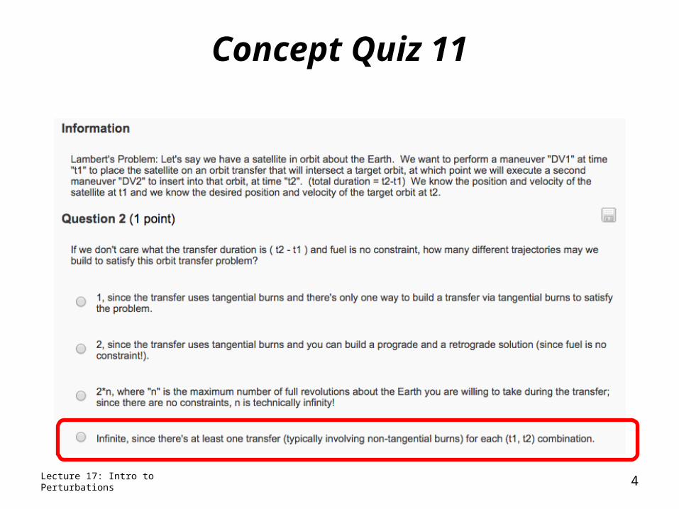
Concept Quiz 11
Lecture 17: Intro to Perturbations 4

Concept Quiz 11
Lecture 17: Intro to Perturbations 5
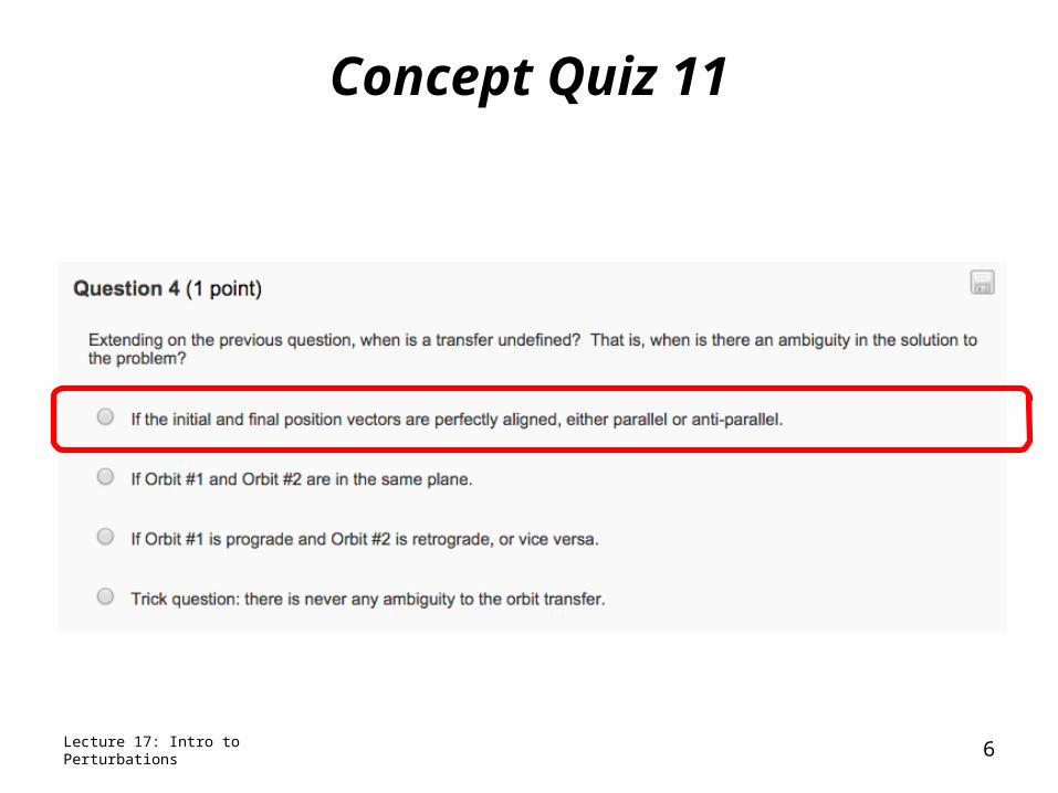
Concept Quiz 11
Lecture 17: Intro to Perturbations 6
Space News
Lecture 17: Intro to Perturbations 7
• Anyone watch the ISS?• Anyone see the lunar eclipse?• There’s an event in 1.5 weeks that is directly related
to the lunar eclipse we just had. Anyone have an idea what the event is?
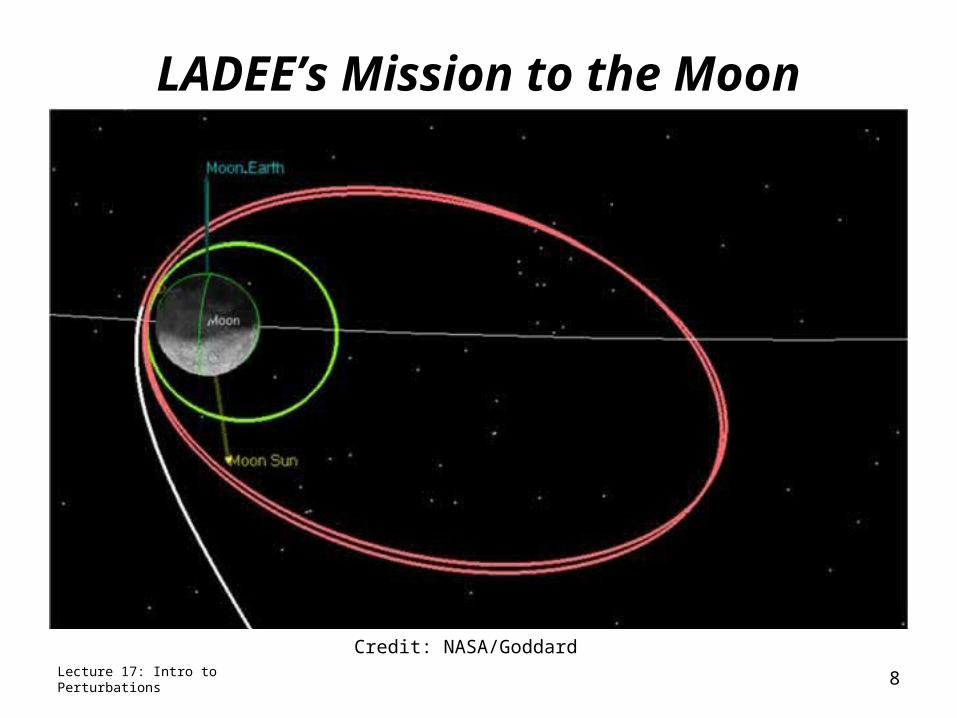
LADEE’s Mission to the Moon• Earth phasing orbits, followed by lunar phasing orbits
Lecture 17: Intro to Perturbations
Credit: NASA/Goddard
8
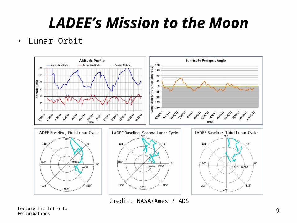
LADEE’s Mission to the Moon• Lunar Orbit
Lecture 17: Intro to Perturbations
Credit: NASA/Ames / ADS
9
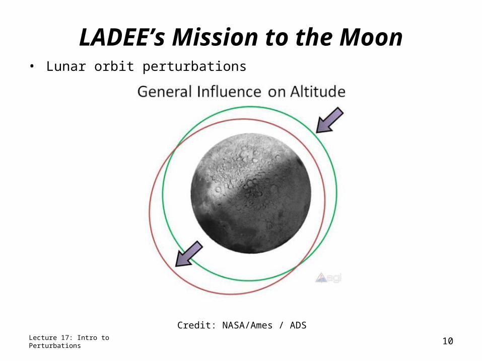
LADEE’s Mission to the Moon• Lunar orbit perturbations
Lecture 17: Intro to Perturbations
Credit: NASA/Ames / ADS
10
ASEN 5050SPACEFLIGHT DYNAMICS
Perturbations
Prof. Jeffrey S. Parker
University of Colorado – Boulder
Lecture 17: Intro to Perturbations 11
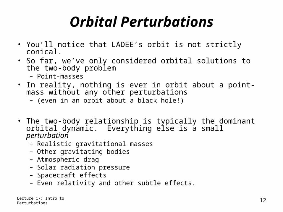
Orbital Perturbations
• You’ll notice that LADEE’s orbit is not strictly conical.• So far, we’ve only considered orbital solutions to the two-body
problem– Point-masses
• In reality, nothing is ever in orbit about a point-mass without any other perturbations – (even in an orbit about a black hole!)
• The two-body relationship is typically the dominant orbital dynamic. Everything else is a small perturbation– Realistic gravitational masses– Other gravitating bodies– Atmospheric drag– Solar radiation pressure– Spacecraft effects– Even relativity and other subtle effects.
Lecture 17: Intro to Perturbations 12
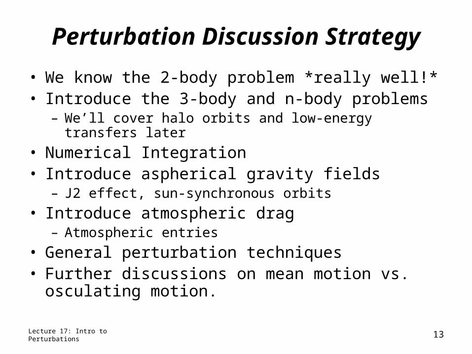
Perturbation Discussion Strategy
• We know the 2-body problem *really well!*• Introduce the 3-body and n-body problems
– We’ll cover halo orbits and low-energy transfers later
• Numerical Integration• Introduce aspherical gravity fields
– J2 effect, sun-synchronous orbits
• Introduce atmospheric drag– Atmospheric entries
• General perturbation techniques• Further discussions on mean motion vs. osculating
motion.
Lecture 17: Intro to Perturbations 13
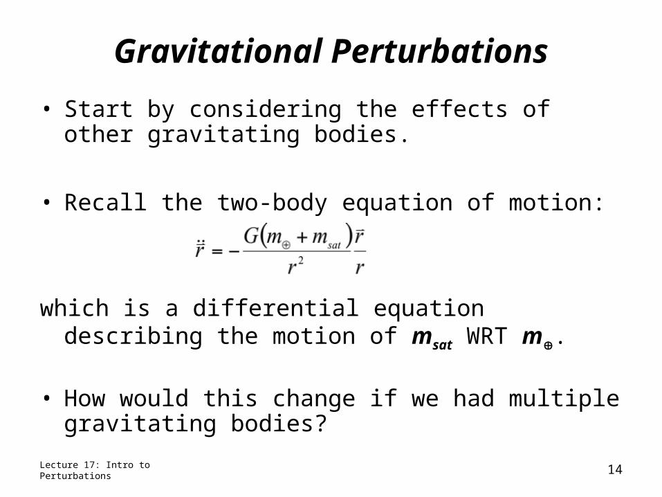
Gravitational Perturbations
• Start by considering the effects of other gravitating bodies.
• Recall the two-body equation of motion:
which is a differential equation describing the motion of msat WRT m.
• How would this change if we had multiple gravitating bodies?
Lecture 17: Intro to Perturbations 14

3-Body Problem
Lecture 17: Intro to Perturbations 15
3-Body Problem
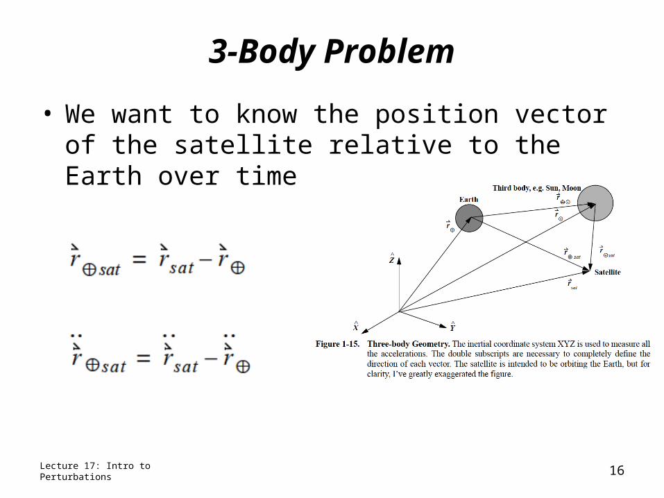
• We want to know the position vector of the satellite relative to the Earth over time
Lecture 17: Intro to Perturbations 16
3-Body Problem
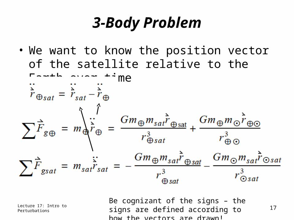
• We want to know the position vector of the satellite relative to the Earth over time
Lecture 17: Intro to Perturbations 17Be cognizant of the signs – the signs are defined according to how the vectors are drawn!
3-Body Problem
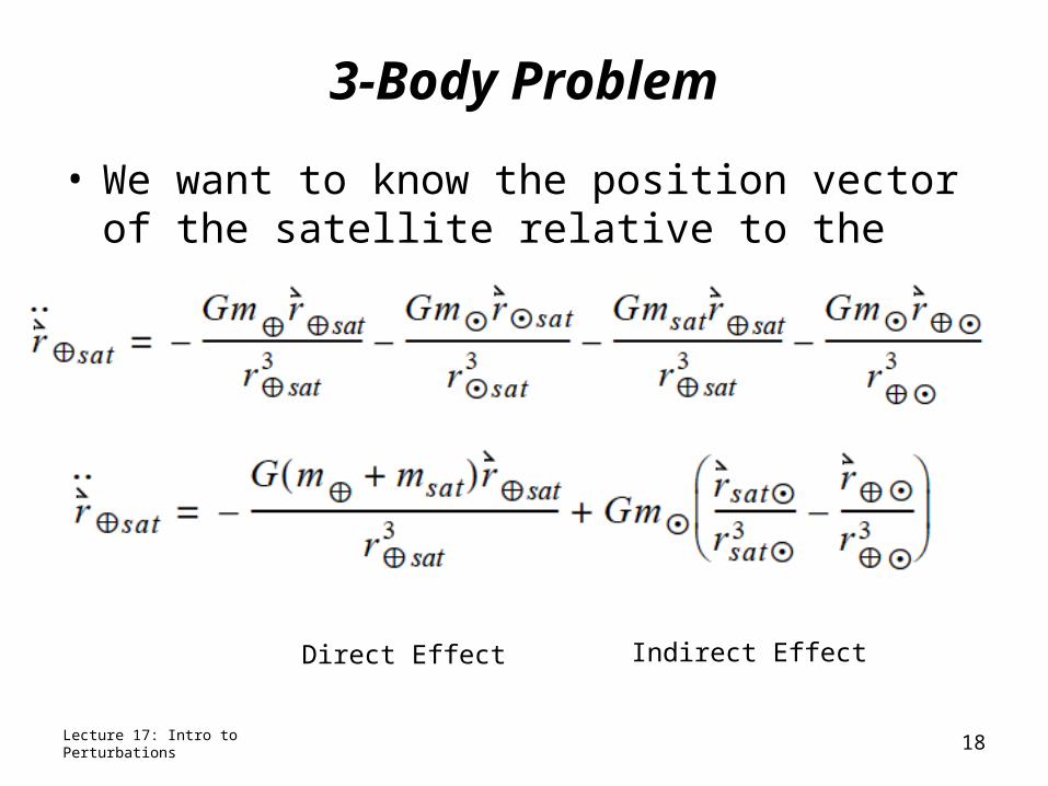
• We want to know the position vector of the satellite relative to the Earth over time
Lecture 17: Intro to Perturbations 18
Direct Effect Indirect Effect
n-Body Problem
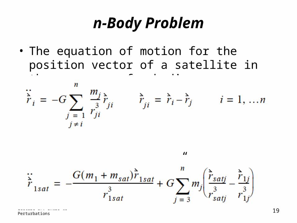
• The equation of motion for the position vector of a satellite in the presence of n bodies.
• … relative to Body “1” (Earth?)
Lecture 17: Intro to Perturbations 19
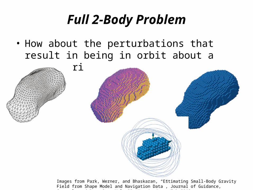
Full 2-Body Problem
• How about the perturbations that result in being in orbit about a non-spherical body?
Images from Park, Werner, and Bhaskaran, “Estimating Small-Body Gravity Field from Shape Model and Navigation Data”, Journal of Guidance, Control, and Dynamics, Vol. 33, No. 1, Jan – Feb 2010.
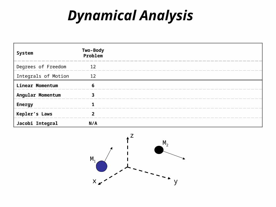
Dynamical Analysis
SystemTwo-Body Problem
Full Three-Body
RTBP: 3rd Body Massless
CRTBP:Circular orbits
PCRTBP (Synodic Frame)
Degrees of Freedom 12 18 18 18 12
Integrals of Motion 12 10 12 13 9
Linear Momentum 6 6 6 6 4
Angular Momentum 3 3 3 3 1
Energy 1 1 1 1 1
Kepler’s Laws 2 0 2 2 2
Jacobi Integral N/A N/A N/A 1 1
x y
M2
M1
z
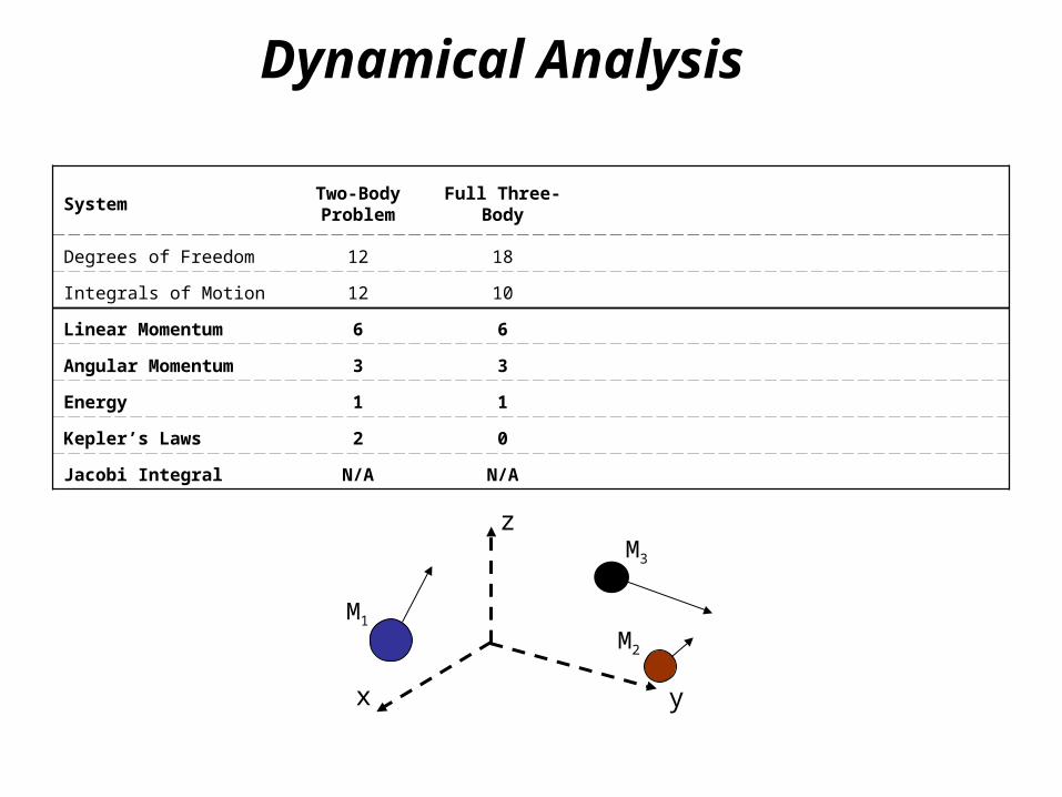
Dynamical Analysis
SystemTwo-Body Problem
Full Three-Body
RTBP: 3rd Body Massless
CRTBP:Circular orbits
PCRTBP (Synodic Frame)
Degrees of Freedom 12 18 18 18 12
Integrals of Motion 12 10 12 13 9
Linear Momentum 6 6 6 6 4
Angular Momentum 3 3 3 3 1
Energy 1 1 1 1 1
Kepler’s Laws 2 0 2 2 2
Jacobi Integral N/A N/A N/A 1 1
x y
M3
M2
M1
z
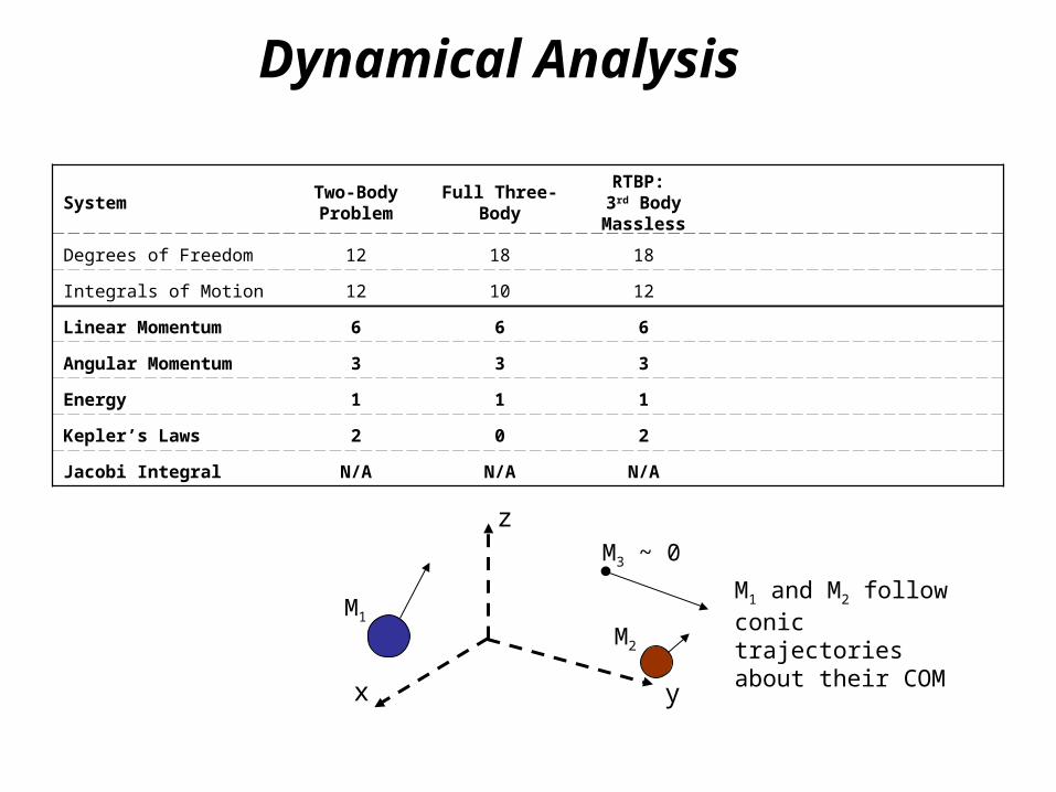
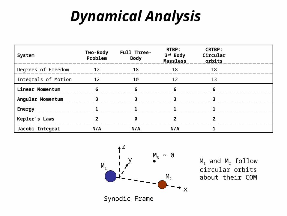
Dynamical Analysis
SystemTwo-Body Problem
Full Three-Body
RTBP: 3rd Body Massless
CRTBP:Circular orbits
PCRTBP (Synodic Frame)
Degrees of Freedom 12 18 18 18 12
Integrals of Motion 12 10 12 13 9
Linear Momentum 6 6 6 6 4
Angular Momentum 3 3 3 3 1
Energy 1 1 1 1 1
Kepler’s Laws 2 0 2 2 2
Jacobi Integral N/A N/A N/A 1 1
x y
M3 ~ 0
M2
M1
z
M1 and M2 follow conic trajectories about their COM
Dynamical Analysis
SystemTwo-Body Problem
Full Three-Body
RTBP: 3rd Body Massless
CRTBP:Circular orbits
PCRTBP (Synodic Frame)
Degrees of Freedom 12 18 18 18 12
Integrals of Motion 12 10 12 13 9
Linear Momentum 6 6 6 6 4
Angular Momentum 3 3 3 3 1
Energy 1 1 1 1 1
Kepler’s Laws 2 0 2 2 2
Jacobi Integral N/A N/A N/A 1 1
y
x
M3 ~ 0
M2
M1
z
M1 and M2 follow circular orbits about their COM
Synodic Frame
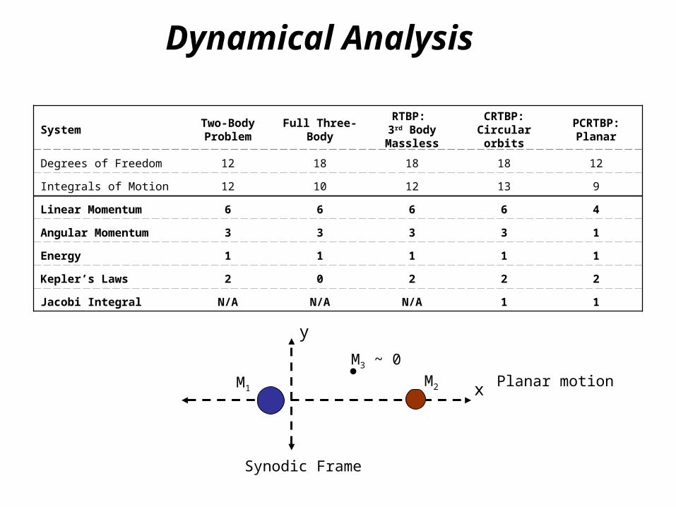
Dynamical Analysis
SystemTwo-Body Problem
Full Three-Body
RTBP: 3rd Body Massless
CRTBP:Circular orbits
PCRTBP: Planar
Degrees of Freedom 12 18 18 18 12
Integrals of Motion 12 10 12 13 9
Linear Momentum 6 6 6 6 4
Angular Momentum 3 3 3 3 1
Energy 1 1 1 1 1
Kepler’s Laws 2 0 2 2 2
Jacobi Integral N/A N/A N/A 1 1
x
M3 ~ 0
M2M1
y
Planar motion
Synodic Frame
Building Solutions to the n-Body Problem
• We have more degrees of freedom than we have integrals of motion!
• Conic sections are no longer solutions.• Most common method used to build solutions to the
n-Body problem is to take initial conditions and integrate them forward in time.– Build a trajectory using knowledge of the equations of
motion.
Lecture 17: Intro to Perturbations 26
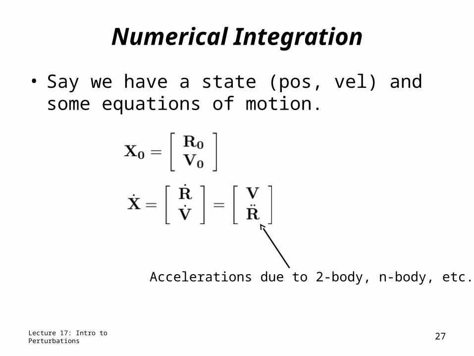
Numerical Integration
• Say we have a state (pos, vel) and some equations of motion.
Lecture 17: Intro to Perturbations 27
Accelerations due to 2-body, n-body, etc.
Numerical Integration
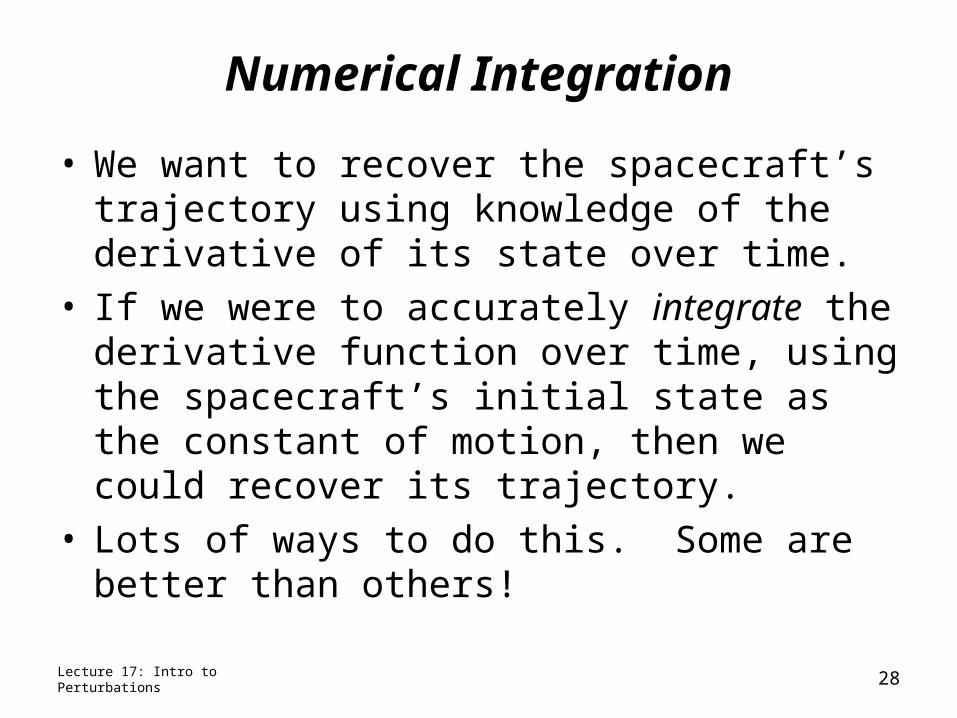
• We want to recover the spacecraft’s trajectory using knowledge of the derivative of its state over time.
• If we were to accurately integrate the derivative function over time, using the spacecraft’s initial state as the constant of motion, then we could recover its trajectory.
• Lots of ways to do this. Some are better than others!
Lecture 17: Intro to Perturbations 28
Numerical Integration
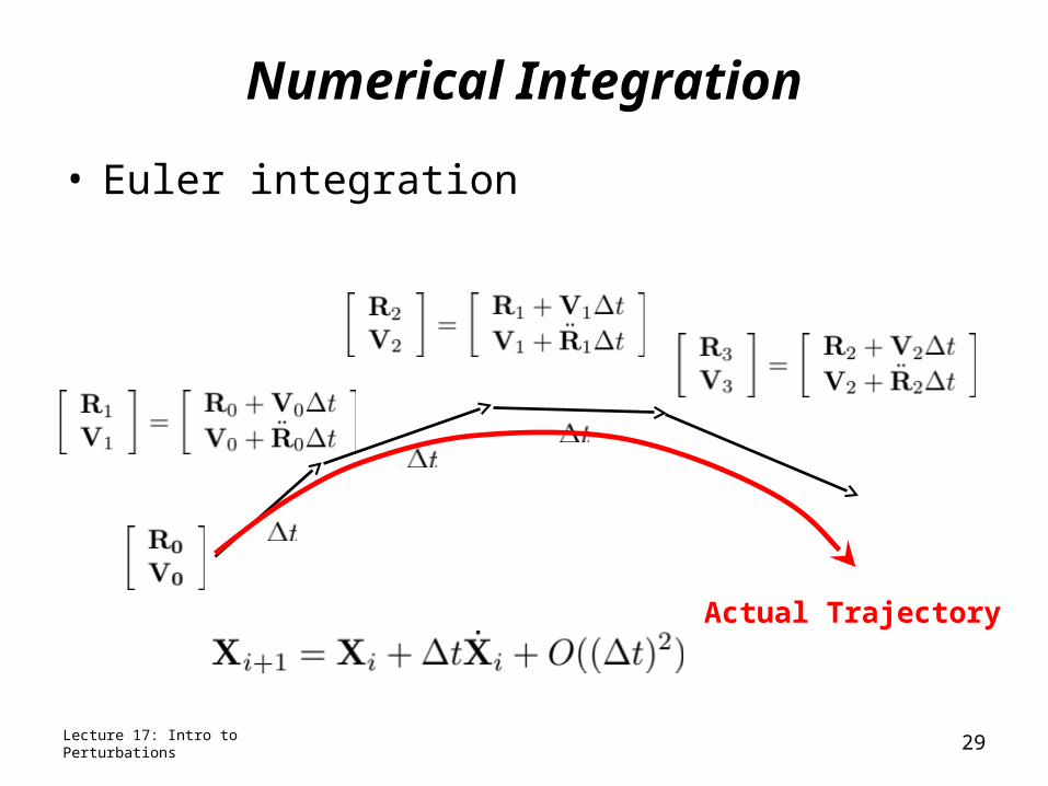
• Euler integration
Lecture 17: Intro to Perturbations 29
Actual Trajectory
Numerical Integration
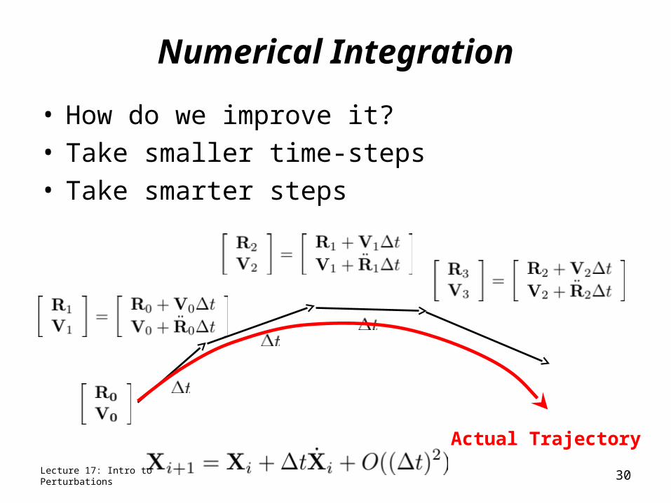
• How do we improve it?• Take smaller time-steps• Take smarter steps
Lecture 17: Intro to Perturbations 30
Actual Trajectory
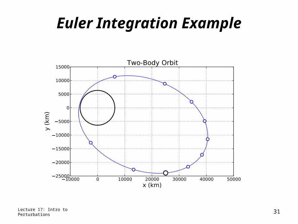
Euler Integration Example
Lecture 17: Intro to Perturbations 31
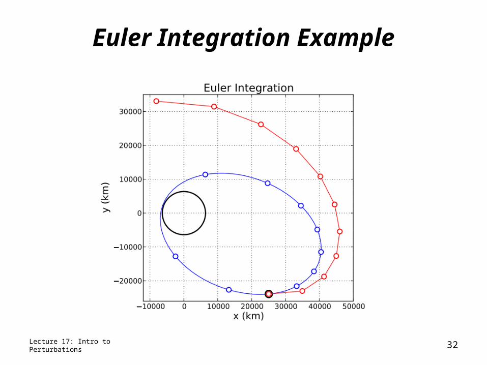
Euler Integration Example
Lecture 17: Intro to Perturbations 32

Euler Integration Example
Lecture 17: Intro to Perturbations 33
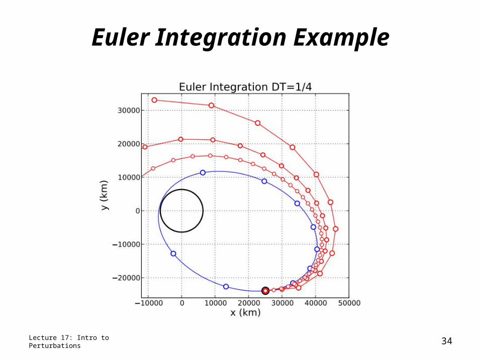
Euler Integration Example
Lecture 17: Intro to Perturbations 34
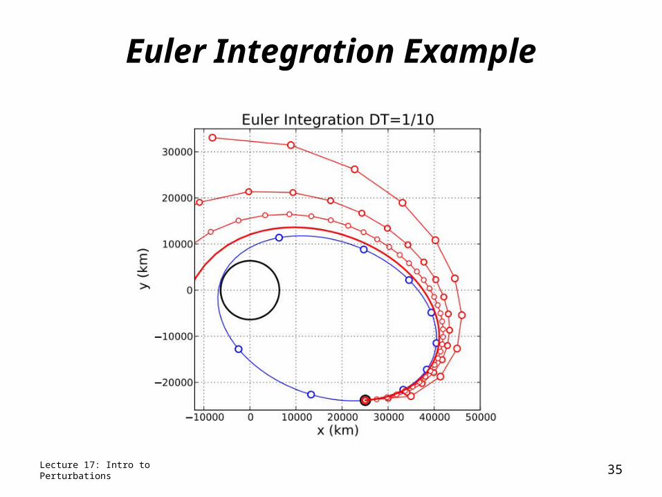
Euler Integration Example
Lecture 17: Intro to Perturbations 35

Euler Integration Example
Lecture 17: Intro to Perturbations 36
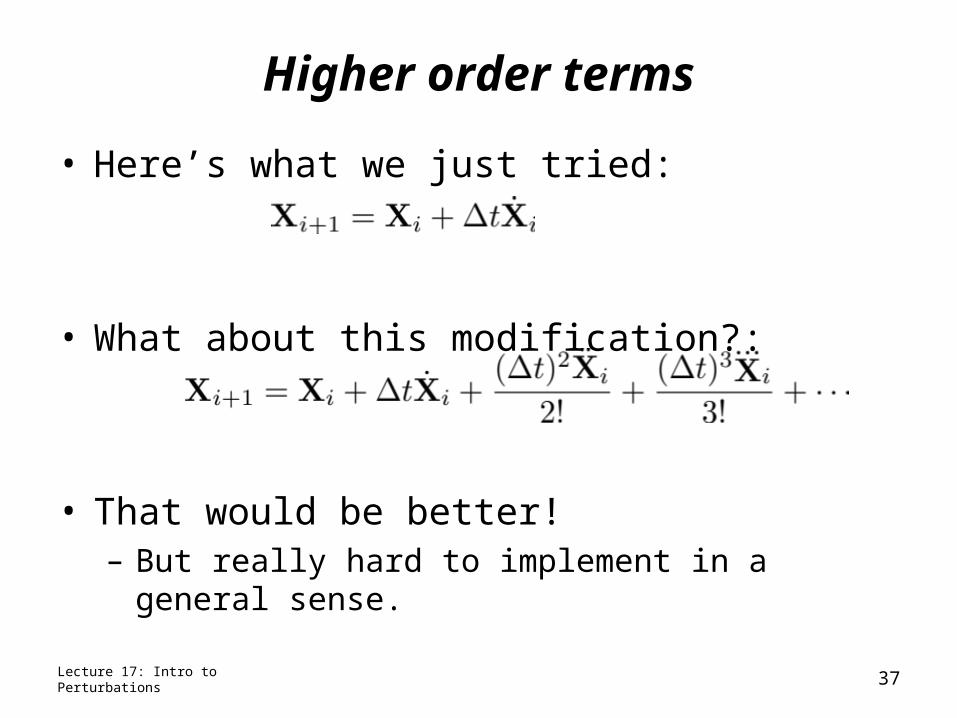
Higher order terms
• Here’s what we just tried:
• What about this modification?:
• That would be better!– But really hard to implement in a general sense.
Lecture 17: Intro to Perturbations 37
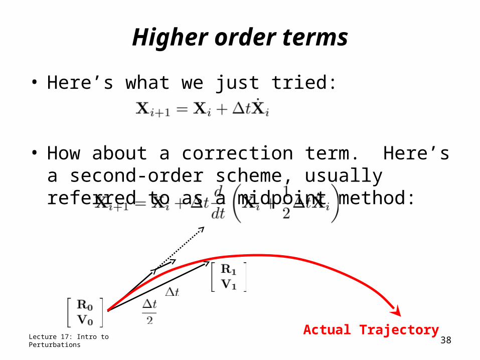
Higher order terms
• Here’s what we just tried:
• How about a correction term. Here’s a second-order scheme, usually referred to as a midpoint method:
Lecture 17: Intro to Perturbations 38Actual Trajectory
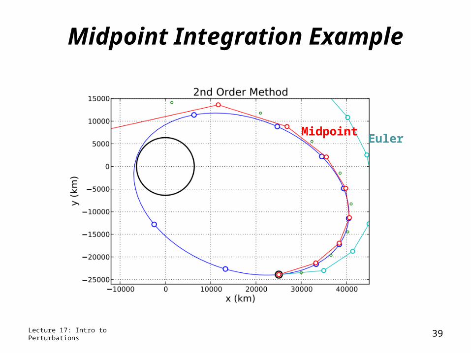
Midpoint Integration Example
Lecture 17: Intro to Perturbations 39
EulerMidpoint
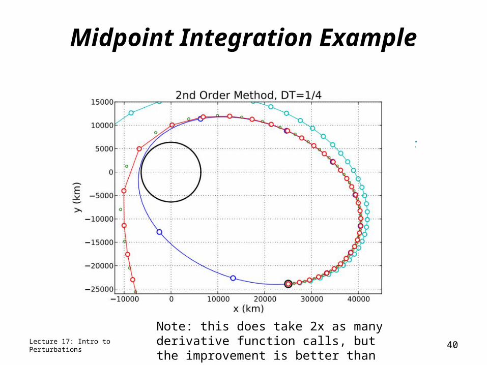
Midpoint Integration Example
Lecture 17: Intro to Perturbations 40
EulerMidpoint
Note: this does take 2x as many derivative function calls, but the improvement is better than just doubling Euler’s!
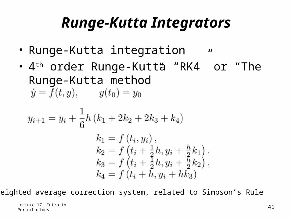
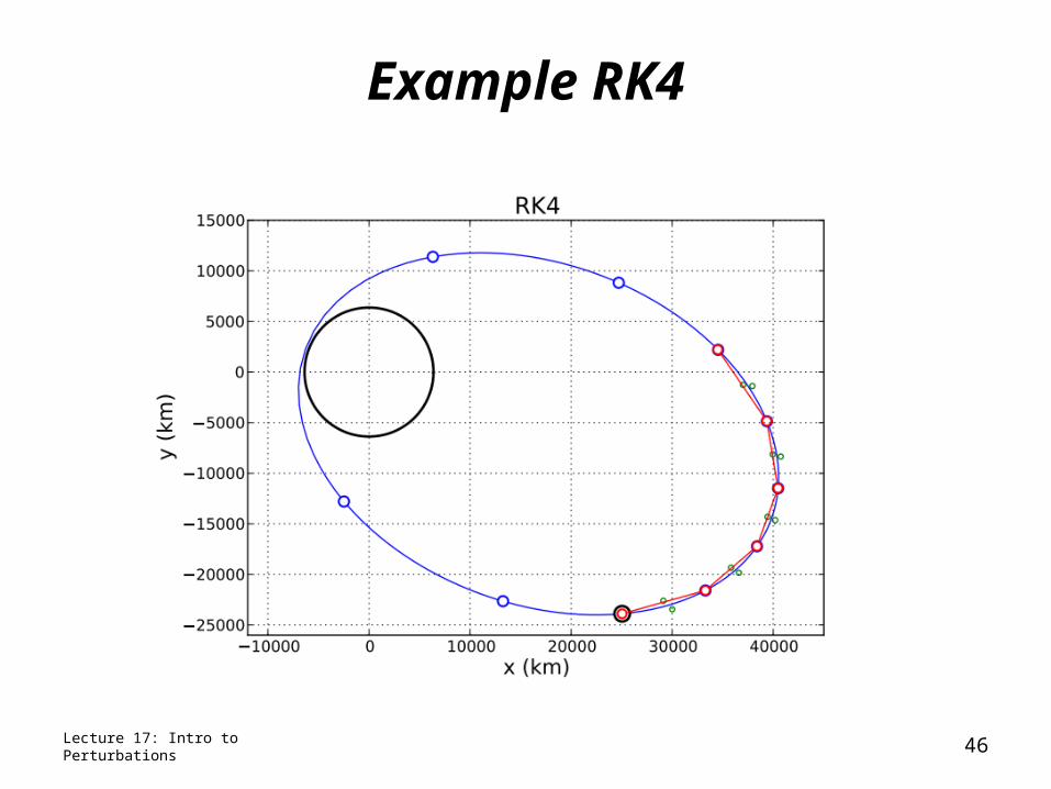
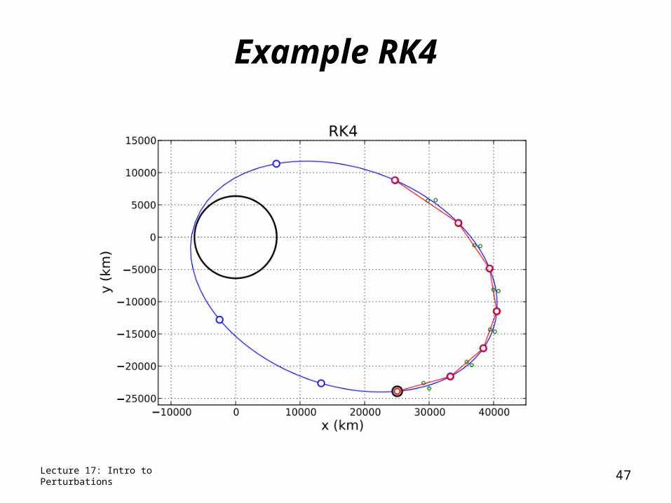
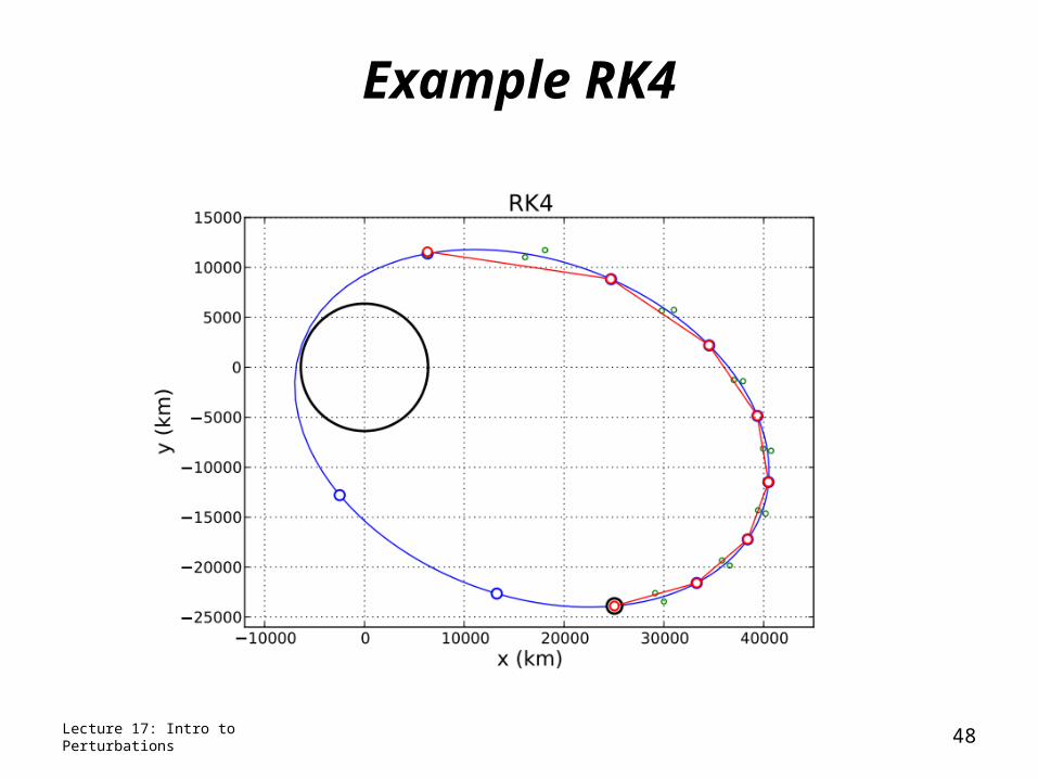
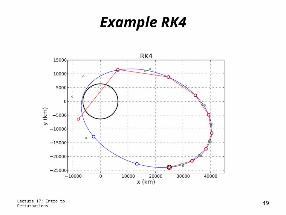
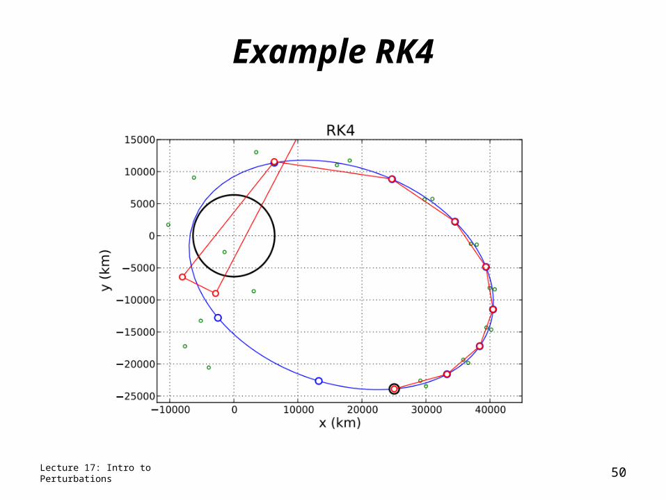
Runge-Kutta Integrators
• Runge-Kutta integration• 4th order Runge-Kutta “RK4” or “The Runge-Kutta
method”
Lecture 17: Intro to Perturbations 41
Weighted average correction system, related to Simpson’s Rule
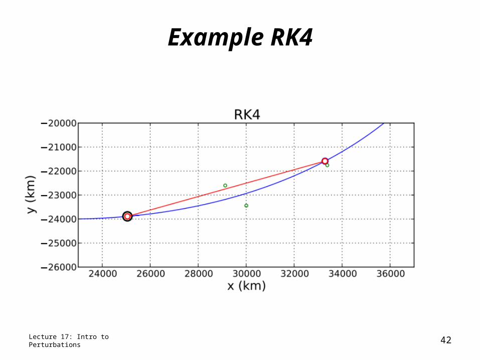
Example RK4
Lecture 17: Intro to Perturbations 42
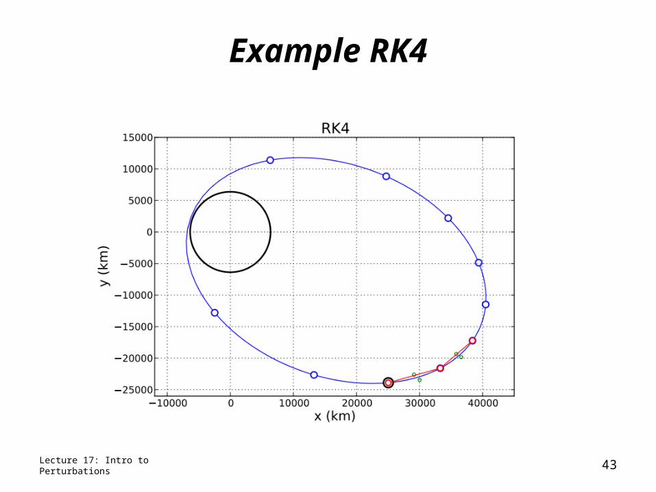
Example RK4
Lecture 17: Intro to Perturbations 43
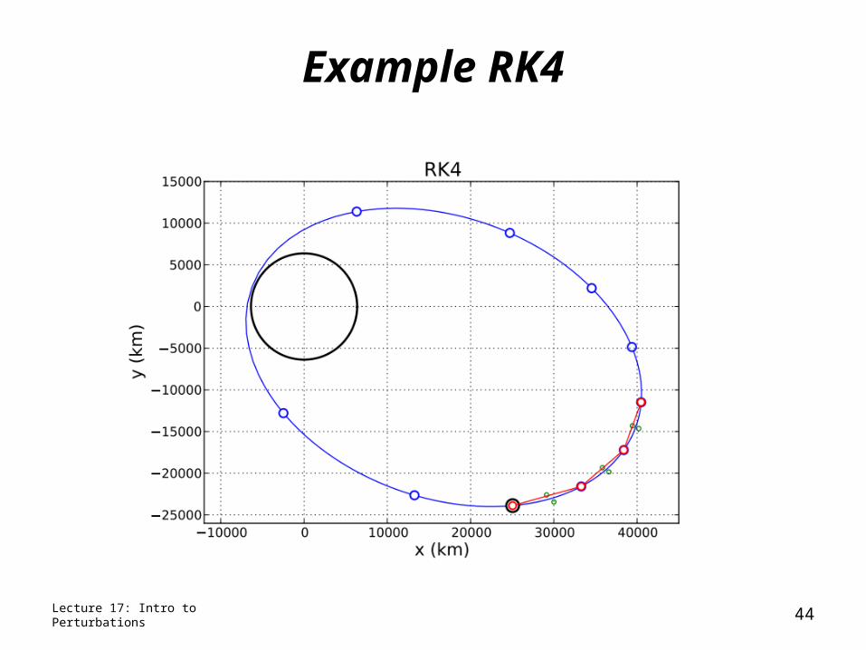
Example RK4
Lecture 17: Intro to Perturbations 44
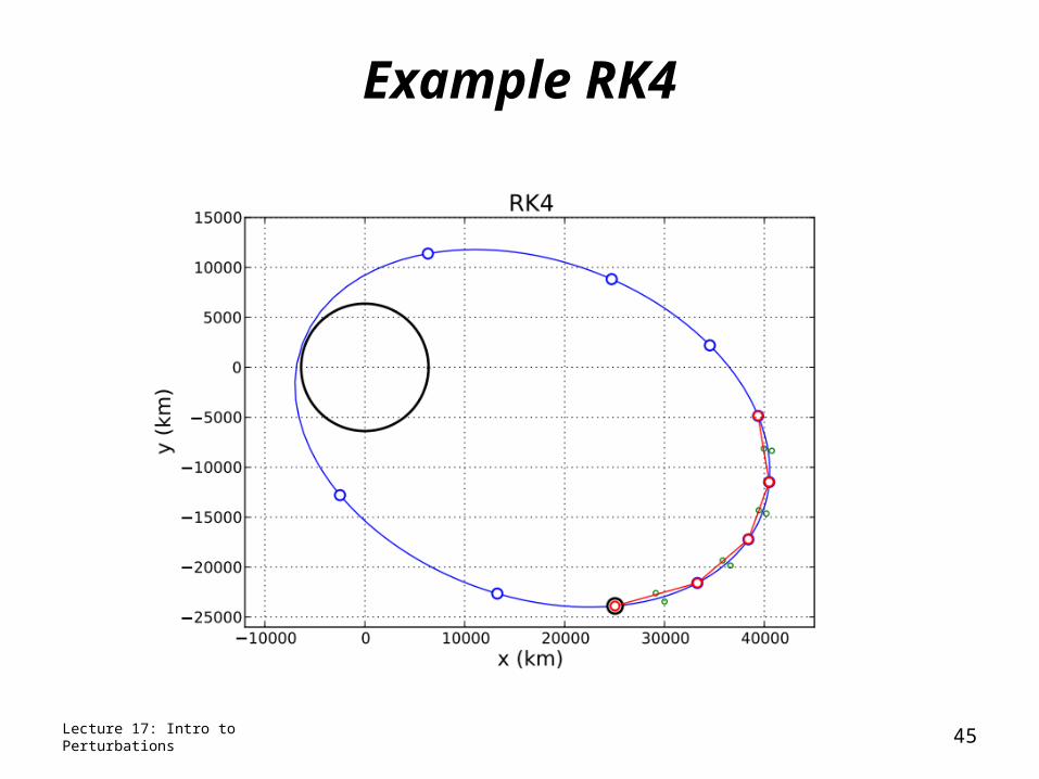
Example RK4
Lecture 17: Intro to Perturbations 45
Example RK4
Lecture 17: Intro to Perturbations 46
Example RK4
Lecture 17: Intro to Perturbations 47
Example RK4
Lecture 17: Intro to Perturbations 48
Example RK4
Lecture 17: Intro to Perturbations 49
Example RK4
Lecture 17: Intro to Perturbations 50
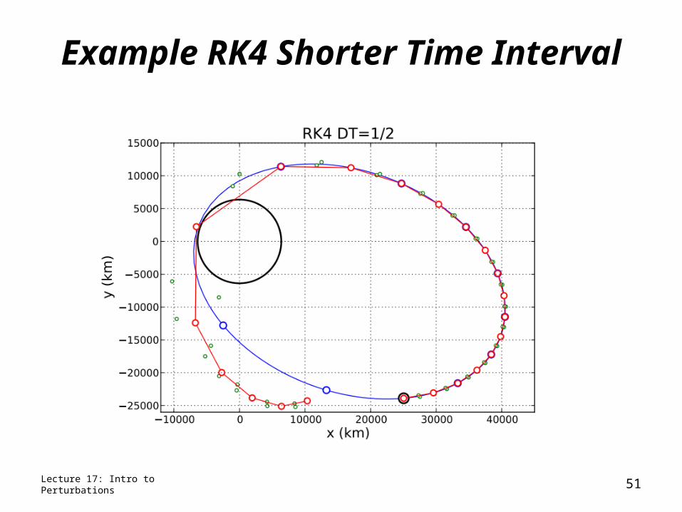
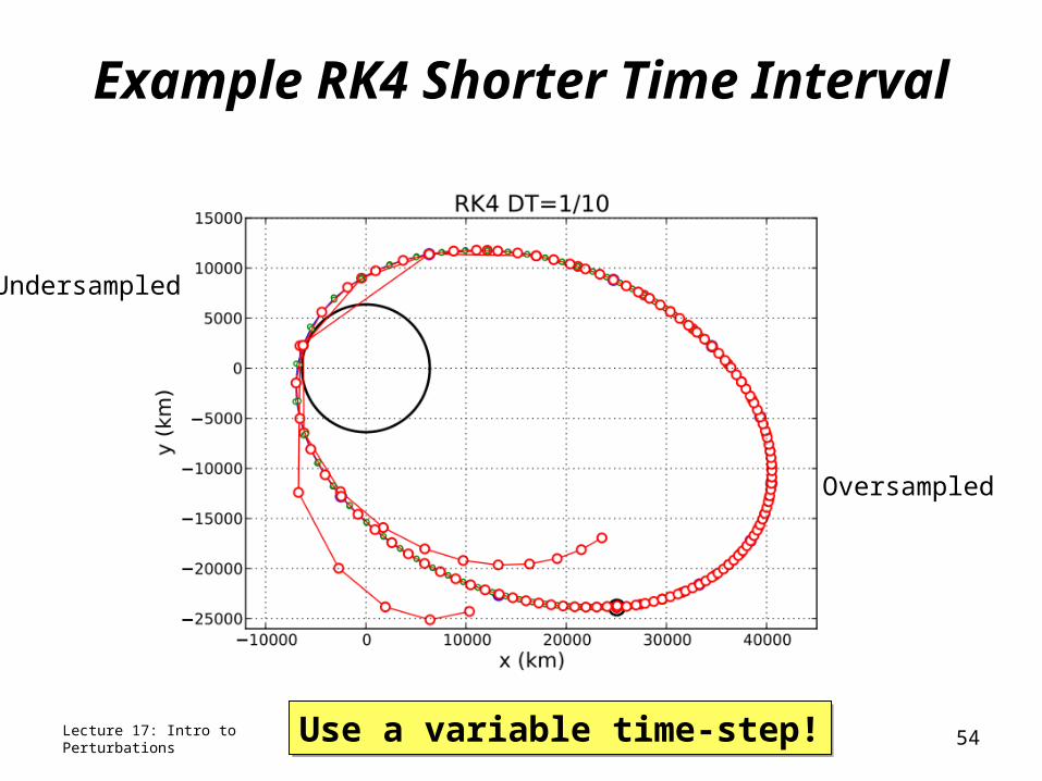
Example RK4 Shorter Time Interval
Lecture 17: Intro to Perturbations 51
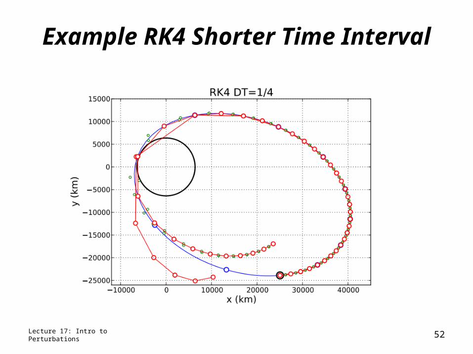
Example RK4 Shorter Time Interval
Lecture 17: Intro to Perturbations 52
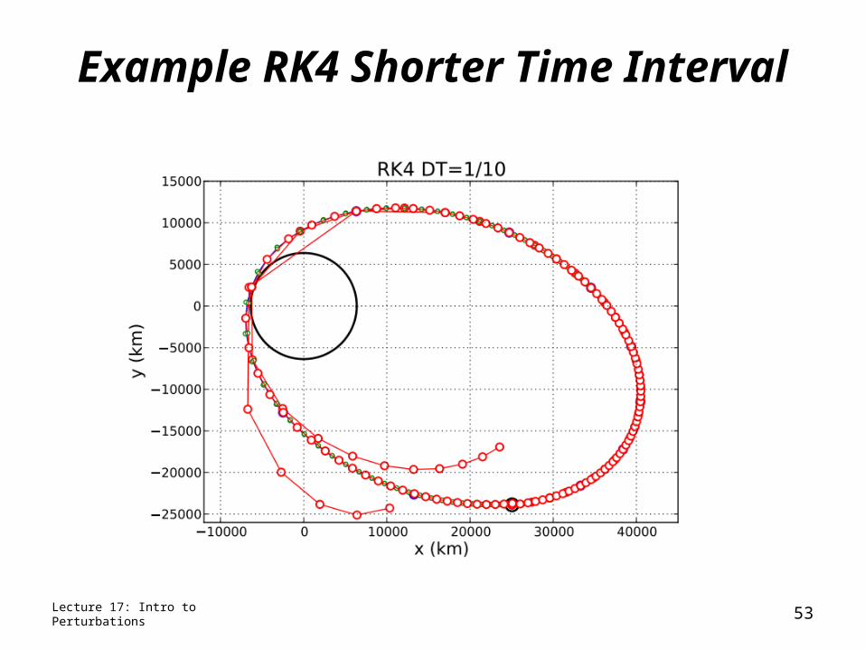
Example RK4 Shorter Time Interval
Lecture 17: Intro to Perturbations 53
Example RK4 Shorter Time Interval
Lecture 17: Intro to Perturbations 54
Oversampled
Undersampled
Use a variable time-step!Use a variable time-step!
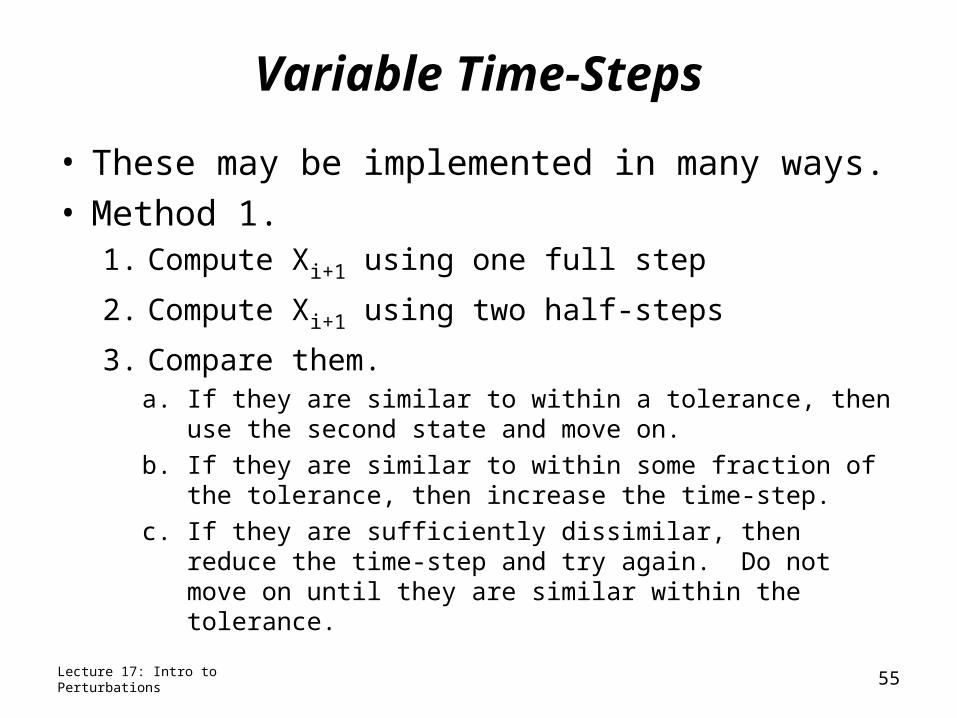
Variable Time-Steps
• These may be implemented in many ways.• Method 1.
1. Compute Xi+1 using one full step
2. Compute Xi+1 using two half-steps
3. Compare them.a. If they are similar to within a tolerance, then use the second state
and move on.
b. If they are similar to within some fraction of the tolerance, then increase the time-step.
c. If they are sufficiently dissimilar, then reduce the time-step and try again. Do not move on until they are similar within the tolerance.
Lecture 17: Intro to Perturbations 55
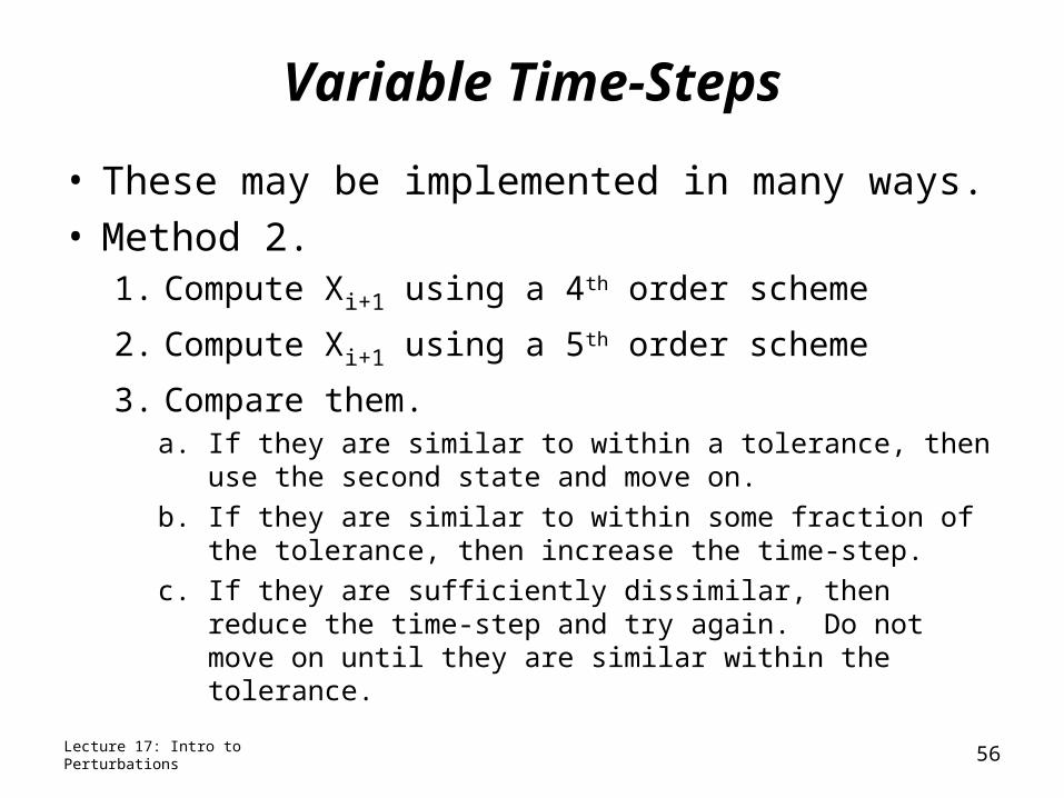
Variable Time-Steps
• These may be implemented in many ways.• Method 2.
1. Compute Xi+1 using a 4th order scheme
2. Compute Xi+1 using a 5th order scheme
3. Compare them.a. If they are similar to within a tolerance, then use the second state
and move on.
b. If they are similar to within some fraction of the tolerance, then increase the time-step.
c. If they are sufficiently dissimilar, then reduce the time-step and try again. Do not move on until they are similar within the tolerance.
Lecture 17: Intro to Perturbations 56
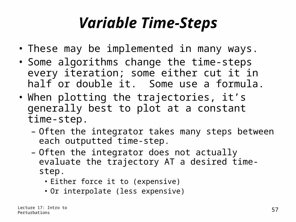
Variable Time-Steps
• These may be implemented in many ways.• Some algorithms change the time-steps every
iteration; some either cut it in half or double it. Some use a formula.
• When plotting the trajectories, it’s generally best to plot at a constant time-step.– Often the integrator takes many steps between each
outputted time-step.– Often the integrator does not actually evaluate the
trajectory AT a desired time-step.• Either force it to (expensive)• Or interpolate (less expensive)
Lecture 17: Intro to Perturbations 57
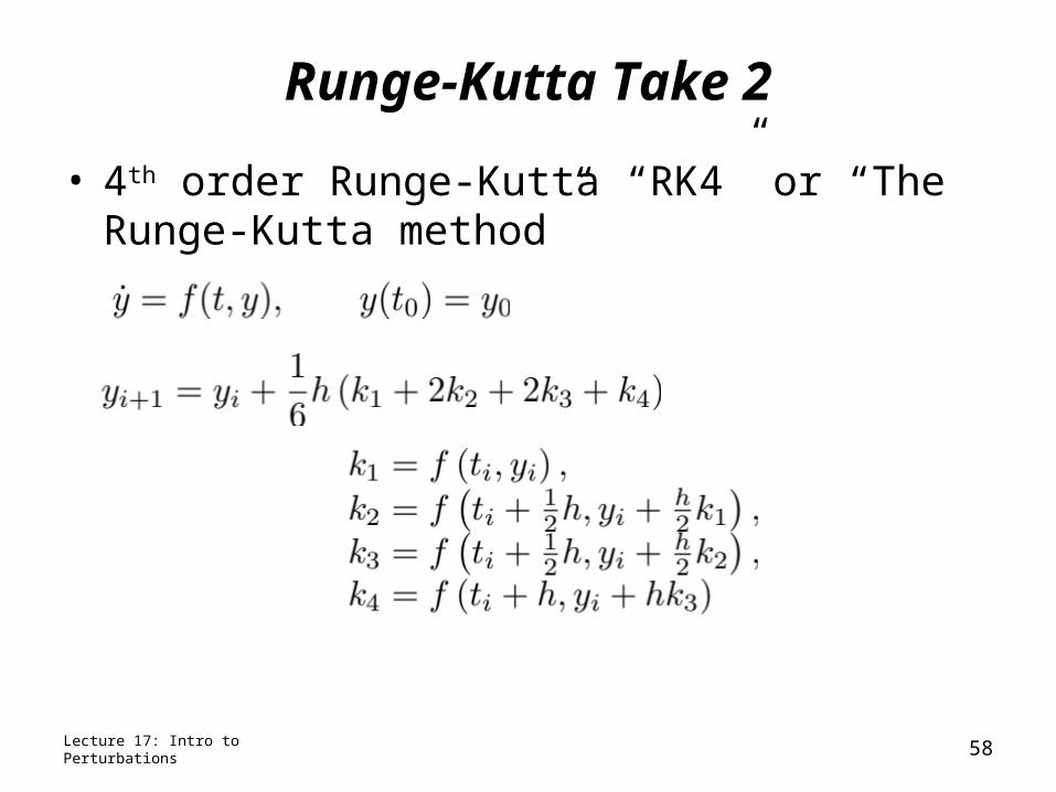
Runge-Kutta Take 2
• 4th order Runge-Kutta “RK4” or “The Runge-Kutta method”
Lecture 17: Intro to Perturbations 58
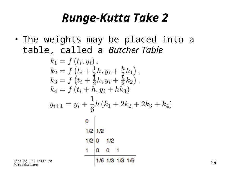
Runge-Kutta Take 2
• The weights may be placed into a table, called a Butcher Table
Lecture 17: Intro to Perturbations 59
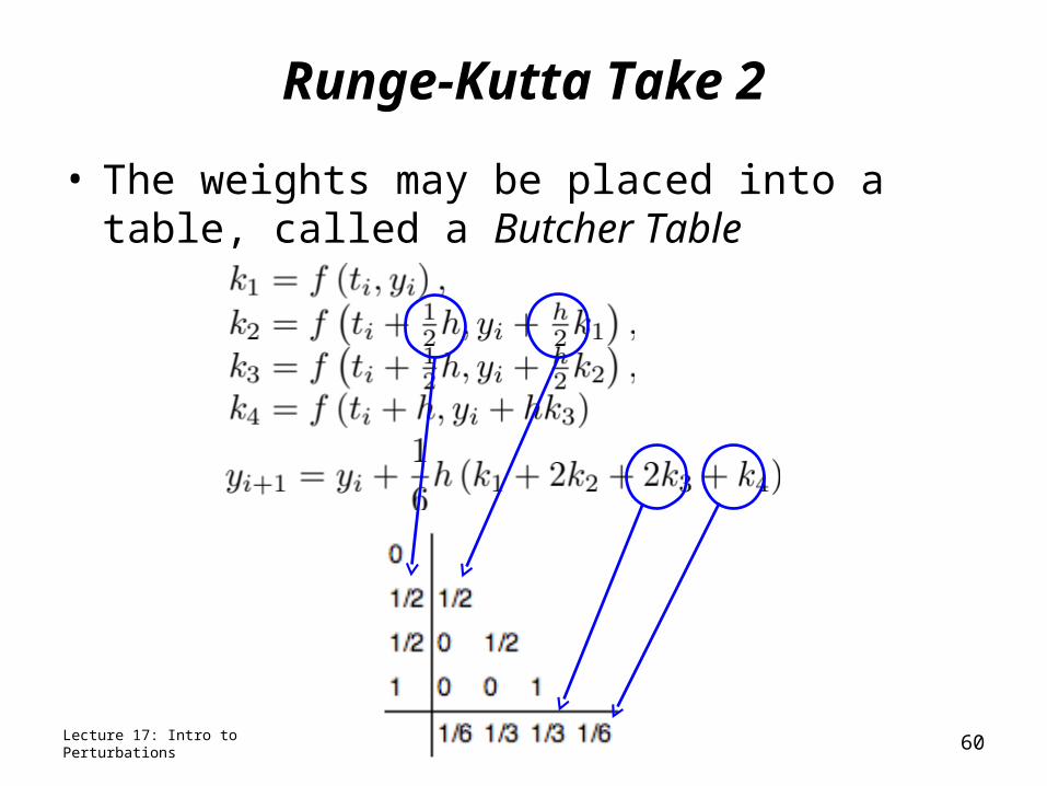
Runge-Kutta Take 2
• The weights may be placed into a table, called a Butcher Table
Lecture 17: Intro to Perturbations 60
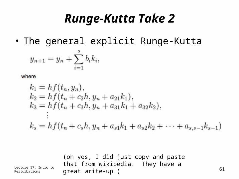
Runge-Kutta Take 2
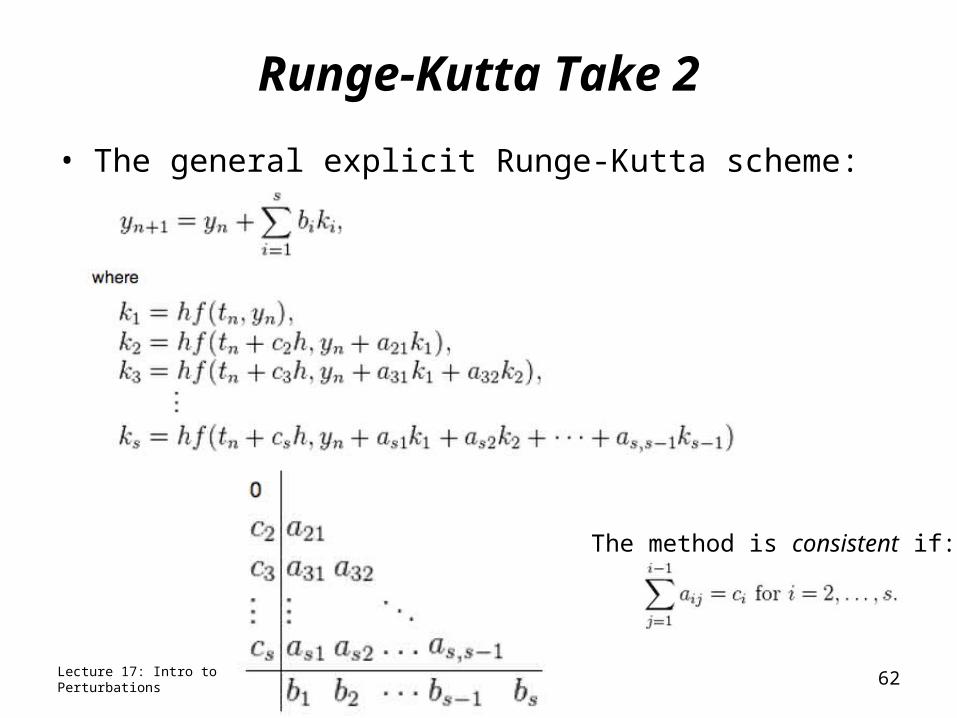
• The general explicit Runge-Kutta scheme:
Lecture 17: Intro to Perturbations 61
(oh yes, I did just copy and paste that from wikipedia. They have a great write-up.)
Runge-Kutta Take 2
• The general explicit Runge-Kutta scheme:
Lecture 17: Intro to Perturbations 62
The method is consistent if:
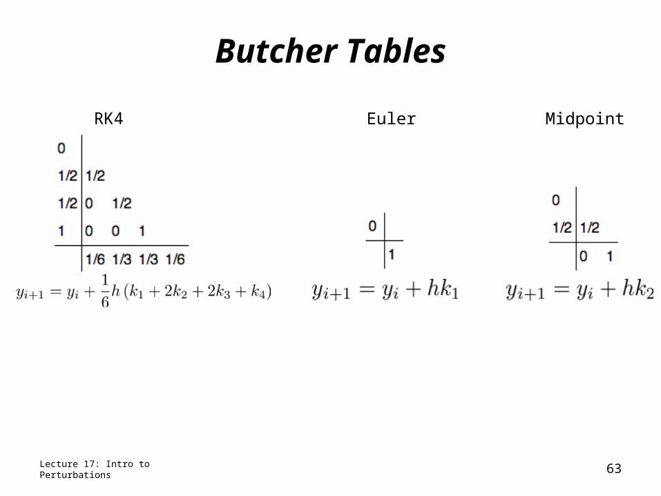
Butcher Tables
Lecture 17: Intro to Perturbations 63
RK4 Euler Midpoint
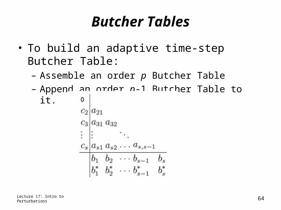
Butcher Tables
• To build an adaptive time-step Butcher Table:– Assemble an order p Butcher Table
– Append an order p-1 Butcher Table to it.
Lecture 17: Intro to Perturbations 64
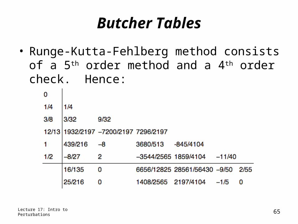
Butcher Tables
• Runge-Kutta-Fehlberg method consists of a 5th order method and a 4th order check. Hence:
Lecture 17: Intro to Perturbations 65
Drawbacks of Explicit RK Methods
• Explicit Runge-Kutta methods are easy to derive and require relatively few computations to implement.
• They are usually quite good for astrodynamic applications.
• Don’t be afraid to use them
• However, for stiff problems they are unstable. They are particularly unstable for solving partial differential equations.
• To combat this, implicit Runge-Kutta methods have been formulated.
Lecture 17: Intro to Perturbations 66
Implicit Runge-Kutta Methods
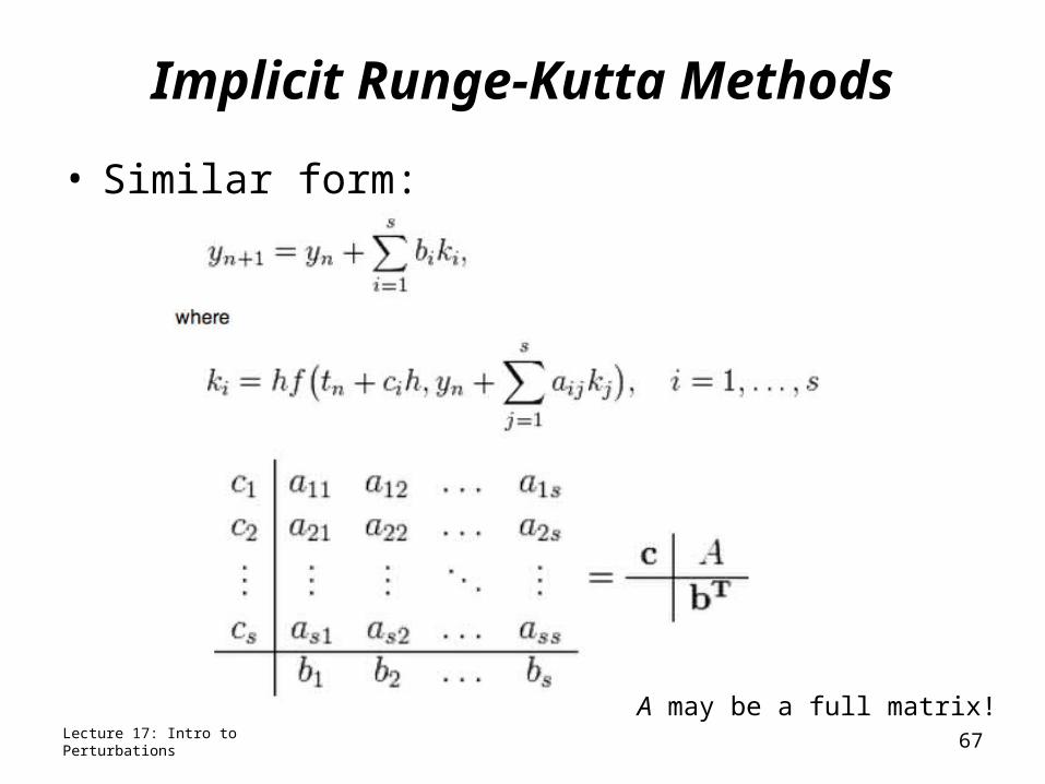
• Similar form:
Lecture 17: Intro to Perturbations 67
A may be a full matrix!
Implicit Runge-Kutta Methods
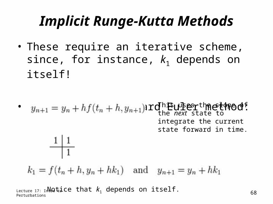
• These require an iterative scheme, since, for instance, k1 depends on itself!
• Example: the backward Euler method:
Lecture 17: Intro to Perturbations 68
This uses the slope of the next state to integrate the current state forward in time.
Notice that k1 depends on itself.
Implicit Runge-Kutta Methods
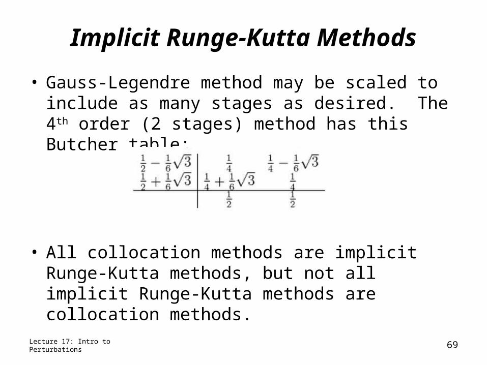
• Gauss-Legendre method may be scaled to include as many stages as desired. The 4th order (2 stages) method has this Butcher table:
• All collocation methods are implicit Runge-Kutta methods, but not all implicit Runge-Kutta methods are collocation methods.
Lecture 17: Intro to Perturbations 69

Announcements
Lecture 17: Intro to Perturbations 70