arXiv:astro-ph/0603522v2 13 Dec 2006 fileMon. Not. R. Astron. Soc. 000, 000–000 (0000) Printed 18...

arX

iv:a

stro

-ph/

0603

522v

2 1

3 D

ec 2

006

Mon. Not. R. Astron. Soc. 000, 000–000 (0000) Printed 18 October 2018 (MN LATEX style file v1.4)

Low surface brightness galaxies rotation curves in the low

energy limit of Rn gravity : no need for dark matter ?

S. Capozziello1, V.F. Cardone2, A. Troisi11 Dipartimento di Scienze Fisiche, Universita degli studi di Napoli “Federico II” and INFN, Sezione di Napoli,Complesso Universitario di Monte S. Angelo, Via Cinthia, Edificio N, 80126 Napoli, Italy2 Dipartimento di Fisica “E.R. Caianiello”, Universita di Salerno,Via S. Allende, 84081 - Baronissi (Salerno), Italy

Accepted xxx, Received yyy, in original form zzz

ABSTRACT

We investigate the possibility that the observed flatness of the rotation curves ofspiral galaxies is not an evidence for the existence of dark matter haloes, but rathera signal of the breakdown of General Relativity. To this aim, we consider power - lawfourth order theories of gravity obtained by replacing the scalar curvature R withf(R) = f0R

n in the gravity Lagrangian. We show that, in the low energy limit, thegravitational potential generated by a pointlike source may be written as Φ(r) ∝

r−1[

1 + (r/rc)β]

with β a function of the slope n of the gravity Lagrangian and rca scalelength depending on the gravitating system properties. In order to apply themodel to realistic systems, we compute the modified potential and the rotation curvefor spherically symmetric and for thin disk mass distributions. It turns out that thepotential is still asymptotically decreasing, but the corrected rotation curve, althoughnot flat, is higher than the Newtonian one thus offering the possibility to fit rotationcurves without dark matter. To test the viability of the model, we consider a sampleof 15 low surface brightness (LSB) galaxies with combined HI and Hα measurementsof the rotation curve extending in the putative dark matter dominated region. We finda very good agreement between the theoretical rotation curve and the data using onlystellar disk and interstellar gas when the slope n of the gravity Lagrangian is set to thevalue n = 3.5 (giving β = 0.817) obtained by fitting the SNeIa Hubble diagram withthe assumed power - law f(R) model and no dark matter. The excellent agreementamong theoretical and observed rotation curves and the values of the stellar mass -to - light ratios in agreement with the predictions of population synthesis models makeus confident that Rn gravity may represent a good candidate to solve both the darkenergy problem on cosmological scales and the dark matter one on galactic scales withthe same value of the slope n of the higher order gravity Lagrangian.

Key words: gravitation – dark matter – galaxies: kinematics and dynamics – galaxies:low surface brightness

1 INTRODUCTION

An impressive amount of unprecedented high quality datahave been accumulated in the last decade and have depictedthe new picture of a spatially flat universe with a subcrit-ical matter content and undergoing a phase of acceleratedexpansion. The measurements of cluster properties as themass and correlation function and the evolution with red-shift of their abundance (Eke et al. 1998; Viana et al. 2002;Bachall et al. 2003; Bachall & Bode 2003), the Hubble dia-gram of Type Ia Supernovae (Riess et al. 2004; Astier et al.2006; Clocchiati et al. 2006), optical surveys of large scale

structure (Pope et al. 2005; Cole et al. 2005; Eisenstein et al.2005), anisotropies in the cosmic microwave background (deBernardis et al. 2000; Spergel et al. 2003), cosmic shear fromweak lensing surveys (van Waerbecke et al. 2001; Refregier2003) and the Lyman -α forest absorption (Croft et al. 1999;McDonald et al. 2005) are concordant evidences in favour ofthe radically new scenario depicted above. Interpreting thishuge (and ever increasing) amount of information in theframework of a single satisfactory theoretical model is themain challenge of modern cosmology.

Although it provides an excellent fit to the most of thedata (Tegmark et al. 2004; Seljak et al. 2005; Sanchez et

c© 0000 RAS

http://arxiv.org/abs/astro-ph/0603522v2

2 S. Capozziello et al.

al. 2006), the old cosmological constant (Carroll et al. 1992;Sahni & Starobinski 2000) is affected by serious theoreticalshortcomings that have motivated the search for alternativecandidates generically referred to as dark energy. Ratherthan enumerating the many ideas on the ground (from ascalar field rolling down a suitably chosen self interactionpotential to phantom fields and unified models of dark en-ergy and dark matter), we refer the interested reader to theenlightening reviews available in literature (see, e.g., Pee-bles & Rathra 2003 and Padmanabhan 2003). Here, we onlyremind that dark energy acts as a negative pressure fluidwhose nature and fundamental properties remain essentiallyunknown notwithstanding the great theoretical efforts madeup to now.

Rather than being evidence for the need of some un-known component in the energy budget, the cosmic speedup of a low matter universe may also be considered as afirst signal of breakdown of Einstein General Relativity. Inthis framework, higher order theories of gravity representan interesting opportunity to explain cosmic accelerationwithout the need of any dark energy. In such models, theRicci scalar curvature R in the gravity Lagrangian is re-placed by a generic function f(R) thus leading to modifiedFriedmann equations that can be formally written in theusual form by defining an effective negative pressure curva-

ture fluid driving the cosmic acceleration (Capozziello 2002;Capozziello, Carloni and Troisi 2003; Carroll et al. 2004; No-jiri & Odintsov 2003). Also referred to as f(R) theories, thisapproach has been extensively studied both from the theo-retical (see, e.g., Capozziello, Cardone and Troisi 2005 andrefs. therein) and observational point of view (Capozzielloet al. 2003; Capozziello, Cardone and Francaviglia 2006;Borowiec, Godlowski and Szydlowski 2006). Moreover, thissame approach has been also proposed as a mechanism togive rise to an inflationary era without the need of any in-flaton field (Starobinsky 1980). All these works have beenconcentrated on the cosmological applications of f(R) the-ories and have convincingly demonstrated that they are in-deed able to explain the cosmic speed up and fit the avail-able dataset and hence represents a viable alternative to themysterious dark energy.

Changing the gravity Lagrangian has consequences notonly on cosmological scales, but also at the galactic onesso that it is mandatory to investigate the low energy limitof f(R) theories. Unfortunately, here a strong debate isstill open with different papers drawing contrasting resultsarguing in favour (Dick 2004; Sotiriou 2006; Cembranos2006; Navarro & van Acoleyen 2005; Allemandi et al. 2005;Capozziello & Troisi 2005) or against (Dolgov 2003; Chiba2003; Olmo 2005) such models. It is worth noting that, asa general result, higher order theories of gravity cause thegravitational potential to deviate from its Newtonian 1/rscaling (Stelle 1978; Kluske & Schmidt 1996; Schmidt 2004;Clifton & Barrow 2005; Sobouti 2006) even if such devia-tions may also be very soon vanishing.

In a previous paper (Capozziello et al. 2004), the New-tonian limit of power law f(R) = f0R

n theories has been in-vestigated, assuming that the metric in the low energy limit(Φ/c2 << 1) may be taken as Schwarzschild - like. It turnsout that a power law term (r/rc)

β has to be added to theNewtonian 1/r term in order to get the correct gravitationalpotential. While the parameter β may be expressed analyti-

cally as function of the slope n of the f(R) theory, rc sets thescale where the correction term starts being significant andhas to be determined case - by - case. We then investigated aparticular range of values of n leading to β > 0 so that thecorrective term is an increasing function of the radius r thuscausing an increase of the rotation curve with respect to theNewtonian one and offering the possibility to fit the galaxyrotation curves without the need of the elusive dark mat-ter component. As a preliminary test, we successfully fittedthe Milky Way rotation curve using a model made out ofthe luminous components (bulge and disk) only. Notwith-standing these encouraging results, the corrected potentialfor n in the range explored in our previous paper is, however,troublesome. Indeed, the correction term never switches offso that the total gravitational potential has the unpleasantfeature of being formally divergent as r goes to infinity. Ac-tually, the expression for the gravitational potential has beenobtained in the low energy limit so that cannot be extrap-olated to distances where this approximation does not holdanymore. Nevertheless, for typical values of the parameters(β, rc), the rotation curve starts increasing for values of rnear the visible edge of the disk thus contradicting what isobserved in outer galaxies where the rotation curve is flat orslowly rising (Persic et al. 1996; Catinella et al. 2006).

Elaborating further on the previous results, we presenthere the analysis of the gravitational potential which is ob-tained by considering a different approach to the Newtonianlimit of f(R) theories giving rise to a correction term (r/rc)

γ

with −1 < γ < 0. As we will see, the corresponding rota-tion curve is asymptotically decreasing as in the Newtoniancase, but is nevertheless higher than the standard one sothat it is still possible to fit the data without the need ofdark matter. Moreover, for such models, the gravitationalpotential asymptotically vanishes so that the problem dis-cussed above is avoided. To further substantiate our model,we consider a set of low surface brightness (hereafter LSB)galaxies with extended and well measured rotation curves.Since these systems are supposed to be dark matter domi-nated, successfully fitting our model with no dark matter tothe LSB rotation curves would be a strong evidence in favorof our approach. Combined with the hints coming from thecosmological applications discussed above, we should thushave the possibility to solve both the dark energy and darkmatter problems resorting to the same well motivated funda-mental theory (see (Capozziello, Cardone and Troisi 2006)for preliminary results in this sense).

The plan of the paper is as follows. In Sect. 2, we brieflyresume how the gravitational potential may be obtained inthe low energy limit of power - law f(R) theories in the caseof a pointlike source. The generalization to both a sphericallysymmetric system and a thin disk is presented in Sect. 3. Thedata on the rotation curve, the modelling of LSB galaxiesand the method adopted to determine the model parametersare presented in Sect. 4. An extensive analysis of the fittingprocedure is carried out in Sect. 5 where we use simulatedrotation curves to investigate how parameter degeneraciesaffect the estimate of the model parameters. The results ofthe fit are presented in Sect. 6, while Sect. 7 is devoted tosummarize and foresee future prospects. Some more detailson the fit results on a case - by - case basis and on the smooth-ing procedure are given in Appendix A and B respectively.

c© 0000 RAS, MNRAS 000, 000–000

LSB rotation curves and Rn gravity theories 3

2 LOW ENERGY LIMIT OF F (R) GRAVITY

As yet stated in the introduction, f(R) theories of gravityrepresent a straightforward generalization of the EinsteinGeneral Relativity. To this aim, one considers the action :

A =

∫

d4x√−g [f(R) + Lm] (1)

where f(R) is a generic analytic function of the Ricci scalarcurvature R and Lm is the standard matter Lagrangian.The choice f(R) = R + 2Λ gives the General Relativityincluding the contribution of the cosmological constant Λ.Varying the action with respect to the metric componentsgµν , one gets the generalized Einstein equations that can bemore expressively recast as (Capozziello 2002; Capozziello,Cardone and Troisi 2005) :

Gµν =1

f ′(R)

1

2gµν

[

f(R)−Rf ′(R)]

+ f ′(R);µν

− gµνf′(R)

+T

(m)µν

f ′(R)(2)

where Gµν = Rµν − (R/2)gµν is the Einstein tensor andthe prime denotes derivative with respect to R. The twoterms f ′(R);µν and f ′(R) imply fourth order derivativesof the metric gµν so that these models are also referred toas fourth order gravity. Starting from Eq.(2) and adoptingthe Robertson -Walker metric, it is possible to show that theFriedmann equations may still be written in the usual formprovided that an effective curvature fluid (hence the nameof curvature quintessence) is added to the matter term withenergy density and pressure depending on the choice of f(R).As a particular case, we consider power - law f(R) theories,i.e. we set :

f(R) = f0Rn (3)

with n the slope of the gravity Lagrangian (n = 1 beingthe Einstein theory) and f0 a constant with the dimensionschosen in such a way to give f(R) the right physical dimen-sions. It has been shown that the choice (3), with n 6= 1and standard matter, is able to properly fit the Hubble dia-gram of Type Ia Supernovae without the need of dark energy(Capozziello et al. 2003; Carloni et al. 2005) and could alsobe reconciled with the constraints on the PPN parameters(Capozziello & Troisi 2005).

Here we study the low energy limit⋆ of this class of f(R)theories. Let us consider the gravitational field generated bya pointlike source and solve the field equations (2) in thevacuum case. Under the hypothesis of weak gravitationalfields and slow motions, we can write the spacetime metricas :

ds2 = A(r)dt2 −B(r)dr2 − r2dΩ2 (4)

where dΩ2 = dθ2 + sin2 θdϕ2 is the line element on theunit sphere. It is worth noting that writing Eq.(4) for theweak field metric is the same as assuming implicitly thatthe Jebsen -Birkhoff theorem holds. While this is true in

⋆ Although not rigourously correct, in the following we will usethe terms low energy limit and Newtonian limit as synonymous.

standard General Relativity, it has never been definitivelyproved for f(R) theories. Actually, since for a general f(R)theory the field equations are fourth order, it is quite diffi-cult to show that the only stationary spherically symmetricvacuum solution is Schwarzschild like. However, that thisis indeed the case has been demonstrated for f(R) theoriesinvolving terms like R + R2 with R2 = Rα

βµνR β

α µν withtorsion (Ramaswamy & Yasskin 1979) and for the case ofany invariant of the form R2 also in the case of null tor-sion (Neville 1980). Moreover, the Jebsen -Birkhoff theoremhas been shown to hold also for more complicated theoriesas multidimensional gravity and Einstein -Yang -Mills the-ories (Brodbeck & Straumann 1993; Bronnikov & Melnikov1995). Therefore, although a rigorous demonstration is stillabsent, it is likely that this theorem is still valid for power -

law f(R) theories, at least in an approximated weak version†that is enough for our aims.

To find the two unknown functions A(r) and B(r), wefirst combine the 00 - vacuum component and the trace ofthe field equations (2) in absence of matter :

3f ′(R) +Rf ′(R)− 2f(R) = 0 ,

to get a single equation :

f ′(R)

(

3R00

g00−R

)

+1

2f(R)− 3

f ′(R);00g00

= 0 . (5)

Eq.(5) is completely general and holds whatever is f(R). Itis worth stressing, in particular, that, even if the metric isstationary so that ∂tgµν = 0, the term f ′(R);00 is not van-ishing because of the non-null Christoffel symbols enteringthe covariant derivative. Using Eq.(3), Eq.(5) reduces to :

R00(r) =2n− 1

6nA(r)R(r)− n− 1

2B(r)

dA(r)

dr

d lnR(r)

dr, (6)

while the trace equation reads :

Rn−1(r) =2− n

3nRn(r) . (7)

Note that for n = 1, Eq.(7) reduces to R = 0, which, insertedinto Eq.(6), gives R00 = 0 and the standard Schwarzschildsolution is recovered. In general, expressing R00 and R interms of the metric (4), Eqs.(6) and (7) become a systemof two nonlinear coupled differential equations for the twofunctions A(r) and B(r). A physically motivated hypothesisto search for solutions is

A(r) =1

B(r)= 1 +

2Φ(r)

c2(8)

with Φ(r) the gravitational potential generated by a point-like mass m at the distance r. With the above hypothesis,the vacuum field equations reduce to a system of two differ-ential equations in the only unknown function Φ(r). To bemore precise, we can solve Eq.(6) or (7) to find out Φ(r) andthen use the other relation as a constraint to find solutionsof physical interest. To this aim, let us remember that, as

† It is, for instance, possible that the metric (4) solves the fieldequations only up to terms of low order in Φ/c2 with Φ thegravitational potential. For the applications we are interested in,Φ/c2 << 1, such weak version of the Jebsen -Birkhoff theoremshould be verified.

c© 0000 RAS, MNRAS 000, 000–000


well known, f(R) theories induces modifications to the grav-itational potential altering the Newtonian 1/r scaling (Stelle1978; Kluske & Schmidt 1996; Schmidt 2004; Clifton & Bar-row 2005). We thus look for a solution for the potential thatmay be written as :

Φ(r) = −Gm2r

[

1 +(

r

rc

)β]

(9)

so that the gravitational potential deviates from the usualNewtonian one because of the presence of the second term onthe right hand side. Note that, when β = 0, the Newtonianpotential is recovered and the metric reduces to the classicalSchwarzschild one. On the other hand, as we will see, itis just this term that offers the intriguing possibility to fitgalaxy rotation curves without the need of dark matter.

In order to check whether Eq.(9) is indeed a viable so-lution, we first insert the expression for Φ(r) into Eqs.(6)and (7) which are both solved if :

(n− 1)(β − 3)[

−β(1 + β)V1ηβ−3

]n−1

×[

1 +βV1P0

P1η

]

P1η = 0 (10)

with η = r/rc, V1 = Gm/c2rc and

P0 = 3(β − 3)2n3 − (5β2 − 31β + 48)n2

− (3β2 − 16β + 17)n− (β2 − 4β − 5) , (11)

P1 = 3(β − 3)2(1− β)n3 + (β − 3)2(5β − 7)n2

− (3β3 − 17β2 + 34β − 36)n+ (β2 − 3β − 4)β . (12)

Eq.(10) is identically satisfied for particular values of n andβ. However, there are some simple considerations allow toexclude such values. First, n = 1 must be discarded since,when deriving Eq.(6) from Eq.(5), we have assumed R 6=0 which is not the case for n = 1. Second, the case β =3 may also be rejected since it gives rise to a correctionto the Newtonian potential scaling as η2 so that the totalpotential diverges quadratically which is quite problematic.Finally, the case β = −1 provides a solution only if n > 1.Since we are interested in a solution which works whatevern is, we discard also this case. However, in the limit we areconsidering, it is V1 << 1. For instance, it is V1 ≃ v2c/c

2 ∼10−6 ÷ 10−3 ranging from Solar System to galactic scales,with vc the circular velocity. As a consequence, we can lookfor a further solution of Eq.(10) solving :

P1(n, β)η + βV1P0(n, β) ≃ P1(n, β)η = 0 . (13)

since the second term of Eq.(13) is always negligible for thevalues of n and β in which we are interested. Eq.(13) is analgebraic equation for β as function of n with the followingthree solutions :

β =

3n− 4

n− 112n2 − 7n− 1−

√

p(n)

q(n)

12n2 − 7n− 1 +√

p(n)

q(n)

(14)

with :

p(n) = 36n4 + 12n3 − 83n2 + 50n + 1 ,

q(n) = 6n2 − 4n+ 2 .

It is easy check that, for n = 1, the second expression givesβ = 0, i.e. the approximate solution reduces to the New-tonian one as expected. As a final check, we have insertedback into the vacuum field equations (5) and (7) the modi-fied gravitational potential (9) with

β =12n2 − 7n− 1−

√36n4 + 12n3 − 83n2 + 50n + 1

6n2 − 4n+ 2(15)

finding out that the approximated solution solve the fieldequations up to 10−6 which is more than sufficient in allastrophysical applications which we are going to consider.

Armed with Eqs.(9) and (15), we can, in principle, setconstraints on n by imposing some physically motivated re-quirements to the modified gravitational potential. However,given the nonlinear relation between n and β, in the follow-ing we will consider β and use Eq.(15) to infer n from theestimated β.

As a first condition, it is reasonable to ask that the po-tential does not diverge at infinity. To this aim, we impose :

limr→∞

Φ(r) = 0

which constraints β− 1 to be negative. A further constraintcan be obtained considering the Newtonian potential 1/r asvalid at Solar System scales. As a consequence, since thecorrection to the potential scales as rβ−1, we must imposeβ − 1 > −1 in order to avoid increasing Φ at the SolarSystem scales. In order to not evade these constraints, inthe following, we will only consider solutions with

0 < β < 1 (16)

that, using Eq.(15), gives n > 1 as lower limit on the slopen of the gravity Lagrangian.

While β controls the shape of the correction term, theparameter rc controls the scale where deviations from theNewtonian potential sets in. Both β and rc have to be de-termined by comparison with observations at galactic scales.An important remark is in order here. Because of Eq.(15),β is related to n which enters the gravity Lagrangian. Sincethis is the same for all gravitating systems, as a consequence,β must be the same for all galaxies. On the other hand, thescalelength parameter rc is related to the boundary condi-tions and the mass of the system. In fact, considering thegeneralization of Eq.(9) to extended systems, one has to takecare of the mass distribution and the geometrical configu-rations which can differ from one galaxy to another. As aconsequence, rc turns out to be not a universal quantity, butits value must be set on a case - by - case basis.

Before considering the generalization to extended sys-tems, it is worth evaluating the rotation curve for the point-like case, i.e. the circular velocity vc(r) of a test particle inthe potential generated by the point mass m. For a centralpotential, it is v2c = rdΦ/dr that, with Φ given by Eq.(9),gives :

v2c (r) =Gm

2r

[

1 + (1− β)(

r

rc

)β]

. (17)

c© 0000 RAS, MNRAS 000, 000–000


As it is apparent, the corrected rotation curve is the sumof two terms. While the first one equals half the Newtoniancurve Gm/r, the second one gives a contribution that mayalso be higher than the half classical one. As expected, forβ = 0, the two terms sum up to reproduce the classical re-sult. On the other hand, for β in the range (16), 1− β > 0so that the the corrected rotation curve is higher than theNewtonian one. Since measurements of spiral galaxies ro-tation curves signal a circular velocity higher than what ispredicted on the basis of the observed mass and the Newto-nian potential, the result above suggests the possibility thatour modified gravitational potential may fill the gap betweentheory and observations without the need of additional darkmatter.

It is worth noting that the corrected rotation curve isasymptotically vanishing as in the Newtonian case, whileit is usually claimed that observed rotation curves are flat(i.e., asymptotically constant). However, such a statementshould be not be taken literally. Actually, observations donot probe vc up to infinity, but only up to a maximum radiusRmax showing that the rotation curve is flat within the mea-surement uncertainties. However, this by no way excludesthe possibility that vc goes to zero at infinity. ConsideringEq.(17), if the exponent of the correction term is quite small,the first term decreases in a Keplerian way, while the secondone approaches its asymptotically null value very slowly sothat it can easily mimic an approximately flat rotation curvein agreement with observations.

3 EXTENDED SYSTEMS

The solution (9) has been obtained in the case of a pointlikesource, but may be easily generalized to the case of extendedsystems. To this aim, we may simply divide the system ininfinitesimal elements with mass dm and add the differentcontributions. In the continuous limit, the sum is replaced byan integral depending on the mass density and the symmetryof the system spatial configuration. Once the gravitationalpotential has been obtained, the rotation curve may be easilyevaluated and then compared with observations.

3.1 Spherically symmetric systems

The generalization of Eq.(9) to a spherically symmetric sys-tem is less trivial than one would expect. In the case of theNewtonian gravitational potential, the Gauss theorem en-sures us that the flux of the gravitational field generated bya point mass m through a closed surface only depends onthe mass m and not on the position of the mass inside thesurface. Moreover, the force on a point inside the surfacedue to sources outside the surface vanishes. As a result, wemay imagine that the whole mass of the system is concen-trated in its centre and, as a consequence, the gravitationalpotential has the same formal expression as for the pointlikecase provided one replaces m with M(r), being this latterquantity the mass within a distance r from the centre.

From a mathematical point of view, we can write in theNewtonian case :

ΦN (r) = −G∫

ρ(x′)

|x− x′|d3x′

= −4πG

r

∫

∞

0

ρ(r′)r′2dr′

= −GM(r)

r

where, in the second row, we have used the Gauss theorem totake the |x− x′|−1 outside the integral sign (considering allthe mass concentrated in the point x′ = 0) and then limitedthe integral to r since points with r′ > r do not contributeto the gravitational force.

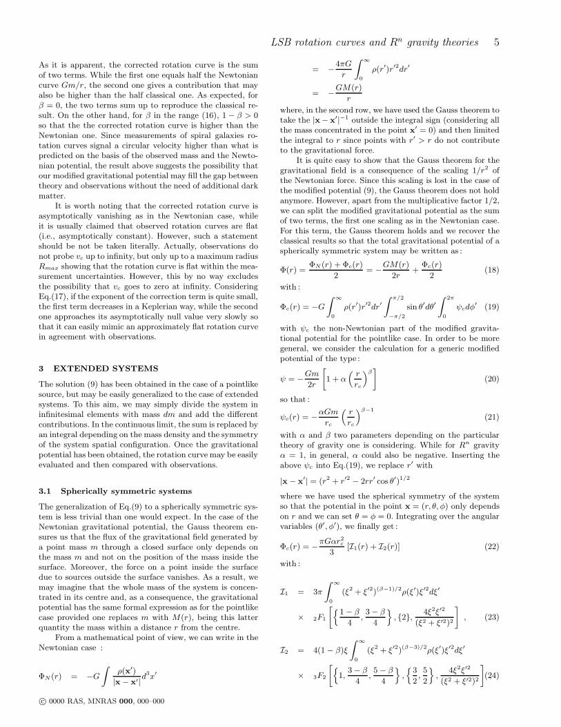
It is quite easy to show that the Gauss theorem for thegravitational field is a consequence of the scaling 1/r2 ofthe Newtonian force. Since this scaling is lost in the case ofthe modified potential (9), the Gauss theorem does not holdanymore. However, apart from the multiplicative factor 1/2,we can split the modified gravitational potential as the sumof two terms, the first one scaling as in the Newtonian case.For this term, the Gauss theorem holds and we recover theclassical results so that the total gravitational potential of aspherically symmetric system may be written as :

Φ(r) =ΦN (r) + Φc(r)

2= −GM(r)

2r+

Φc(r)

2(18)

with :

Φc(r) = −G∫

∞

0

ρ(r′)r′2dr′∫ π/2

−π/2

sin θ′dθ′∫ 2π

0

ψcdφ′ (19)

with ψc the non-Newtonian part of the modified gravita-tional potential for the pointlike case. In order to be moregeneral, we consider the calculation for a generic modifiedpotential of the type :

ψ = −Gm2r

[

1 + α(

r

rc

)β]

(20)

so that :

ψc(r) = −αGmrc

(

r

rc

)β−1

(21)

with α and β two parameters depending on the particulartheory of gravity one is considering. While for Rn gravityα = 1, in general, α could also be negative. Inserting theabove ψc into Eq.(19), we replace r′ with

|x− x′| = (r2 + r′2 − 2rr′ cos θ′)1/2

where we have used the spherical symmetry of the systemso that the potential in the point x = (r, θ, φ) only dependson r and we can set θ = φ = 0. Integrating over the angularvariables (θ′, φ′), we finally get :

Φc(r) = −πGαr2c

3[I1(r) + I2(r)] (22)

with :

I1 = 3π

∫

∞

0

(ξ2 + ξ′2)(β−1)/2ρ(ξ′)ξ′2dξ′

× 2F1

[

1− β

4,3− β

4

, 2, 4ξ2ξ′2

(ξ2 + ξ′2)2

]

, (23)

I2 = 4(1− β)ξ

∫

∞

0

(ξ2 + ξ′2)(β−3)/2ρ(ξ′)ξ′2dξ′

× 3F2

[

1,3− β

4,5− β

4

,

3

2,5

2

,4ξ2ξ′2

(ξ2 + ξ′2)2

]

,(24)

c© 0000 RAS, MNRAS 000, 000–000


and we have generically defined ξ = r/rc and used the nota-tion pF1[a1, . . . , ap, b1, . . . , bq, x] for the hypergeometricfunctions.

Eqs.(23) and (24) must be evaluated numerically for agiven expression of the mass density ρ(r). Once Φc(r) hasbeen evaluated, we can compute the rotation curve as :

v2c (r) = r∂Φ

∂r=v2c,N (r)

2+r

2

∂Φc

∂r(25)

with v2c,N(r) = GM(r)/r the Newtonian rotation curve.Since we are mainly interested in spiral galaxies withoutany spherical component, we do not evaluate the rotationcurve explicitly. We only note that, since Φc has to be eval-uated numerically, in order to avoid numerical derivatives, itis better to first differentiate analytically the expressions forI1 and I2 and then integrate numerically the correspondingintegrals. It is easy to check that the resulting rotation curveis typically slowly decreasing so that it vanishes asymptoti-cally as in the Newtonian case. However, the rate of declineis slower than the Keplerian one so that the total rotationcurve turns out to be higher than the Newtonian one: thisfact allows to fit galaxy rotation curves without the need of

any dark matter halo‡.

3.2 Thin disk

The case of a disk - like system is quite similar to the previousone and, indeed, the gravitational potential may be deter-mined following the same method as before simply takingcare of the cylindrical rather than spherical symmetry ofthe mass configuration. In order to simplify computations,but still dealing with realistic systems, we will consider acircularly symmetric and infinitesimally thin disk and de-

note by Σ(R) its surface mass density§ and by Rd its scalelength. Note that a thin circular disk is the standard choicein describing spiral galaxies so that the model we consideris indeed the most realistic one.

Adopting cylindrical coordinates (R,φ, z), the gravita-tional potential may be evaluated as :

Φ(R, z) =

∫

∞

0

Σ(R′)R′dR′

∫ 2π

0

ψ(|x− x′|)dφ′ (26)

with ψ the pointlike potential and :

|x− x′|2 =

[

(R+R′)2 + z2] [

1− k2 cos2 (φ′/2)]

, (27)

k2 ≡ 4RR′

[(R +R′)2 + z2]. (28)

Inserting Eq.(20) into Eq.(26), we get an integral that canbe split into two additive terms. The first one is half theusual Newtonian one that can be solved using standard pro-cedure (Binney & Tremaine 1987) and therefore will not be

‡ It is worth stressing, at this point, that general conservationlaws are guaranteed by Bianchi identities which hold for genericf(R), so the non-validity of Gauss theorem is not a shortcomingsince we are considering the low energy limit of the theory.§ Here, R is the cylindrical coordinate in the plane of the disk(i.e., R2 = x2 + y2) to be not confused with the Ricci scalarcurvature.

considered anymore. The second one is the correction term

Φc that reads¶ :

Φc(R, z) = −αGΣ0rc

∫

∞

0

Σ(ξ′)[

(ξ + ξ′)2 + ζ2]

β−1

2 ξ′dξ′

×∫ 2π

0

[

1− k2 cos2 (φ′/2)]

β−1

2 dφ′ (29)

with Σ0 = Σ(R = 0), Σ = Σ/Σ0, ξ = R/rc and ζ = z/rc.Integrating over dφ′ and using Eq.(28), we finally get :

Φc(R, z) = −2β−2παGΣ0rcξβ−1

2

∫

∞

0

dξ′Σ(ξ′)ξ′1+β

2

× 2F1

[

1

2,1− β

2

, 1, k2]

k1−β . (30)

Eq.(30) makes it possible to evaluate the corrective term tothe gravitational potential generated by an infinitely thindisk given its surface density Σ(ξ). As a useful application,we consider the case of the exponential disk (Freeman 1970) :

Σ(R) = Σ0 exp (−R/Rd) (31)

with Rd the scale radius. With this expression for the surfacedensity, the corrective term in the gravitational potentialmay be conveniently written as :

Φc(R, z) = −2β−2η−βc παGΣ0Rdη

β−1

2

∫

∞

0

dη′e−η′

η′β+1

2

× 2F1

[

1

2,1− β

2

, 1, k2]

k1−β (32)

with η = R/Rd and ηc = rc/Rd and k is still given byEq.(28) replacing (R,R′, z) with (η, η′, z/Rd). The rotationcurve for the disk may be easily computed starting from theusual relation (Binney & Tremaine 1987) :

v2c (R) = R∂Φ(R, z)

∂R

∣

∣

∣

∣

z=0

= η∂Φ(R, z)

∂η

∣

∣

∣

∣

z/Rd=0

. (33)

Inserting the total gravitational potential into Eq.(33), wemay still split the rotation curve in two terms as :

v2c (R) =v2c,N (R) + v2c,corr(R)

2(34)

where the first term is the Newtonian one, which for anexponential disk reads (Freeman 1970) :

v2c,N(R) = 2πGΣ0Rd(η/2)2

× [I0(η/2)K0(η/2) − I1(η/2)K1(η/2)] (35)

with Il,Kl Bessel functions of order l of the first and sec-ond type respectively. The correction term v2c,corr may beevaluated inserting Eq.(32) into Eq.(33). Using :

∂k

∂η=

k

2η

[

1− k2(η + η′)

2η′

]

,

we finally get :

¶ As in the previous paragraph, it is convenient to let apart themultiplicative factor 1/2 and inser it only in the final result sothat the total potential reads Φ(R, z) = [ΦN (R, z) + Φc(R, z)] /2.

c© 0000 RAS, MNRAS 000, 000–000


v2c,corr(η) = −2β−5η−βc πα(β − 1)GΣ0Rdη

β−1

2 Idisk(η, β)(36)

where we have defined :

Idisk(η, β) =

∫

∞

0

F(η, η′, β)k3−βη′β−1

2 e−η′

dη′ (37)

with :

F = 2(η + η′)2F1

[

1

2,1− β

2

, 1, k2]

+[

(k2 − 2)η′ + k2η]

2F1

[

3

2,3− β

2

, 2, k2]

.(38)

The function Idisk(η, β) may not be evaluated analytically,but it is straightforward to estimate it numerically. Note thatEqs.(36) and (37) can be easily generalized to a different

surface density by replacing the term e−η′

with Σ(η′) andRd with Rs, being this latter a typical scale radius of thesystem, while the function F remains unaltered.

4 LSB ROTATION CURVES

Historically, the flatness of rotation curves of spiral galaxieswas the first and (for a long time) more convincing evidencefor the existence of dark matter (Sofue & Rubin 2001). De-spite much effort, however, it is still unclear to what extentbright spiral galaxies may give clues about the properties ofthe putative dark haloes. On the one hand, being poor ingas content, their rotation curves is hardly measured out tovery large radii beyond the optical edge of the disk wheredark matter is supposed to dominate the rotation curve. Onthe other hand, the presence of extended spiral arms andbarred structures may lead to significative non-circular mo-tions thus complicating the interpretation of the data. Onthe contrary, LSB and dwarf galaxies are supposed to bedark matter dominated at all radii so that the details of thevisible matter distribution are less important. In particular,LSB galaxies have an unusually high gas content, represent-ing up to 90% of their baryonic content (van den Hock etal. 2000; Schombert et al. 2001), which makes it possible tomeasure the rotation curve well beyond the optical radiusRopt ≃ 3.2Rd. Moreover, combining 21 - cm HI lines and op-tical emission lines such as Hα and [NII] makes it possible tocorrect for possible systematic errors due to beam smearingin the radio. As a result, LSB rotation curves are nowadaysconsidered a useful tool to put severe constraints on theproperties of the dark matter haloes (see, e.g., de Blok 2005and references therein).

4.1 The data

It is easy to understand why LSB rotation curves are idealtools to test also modified gravity theories. Indeed, success-fully fitting the rotation curves of a whatever dark matterdominated system, without resorting to dark matter, shouldrepresent a serious evidence arguing in favour of modifica-tions of the standard Newtonian potential. In order to testour model, we have therefore considered a sample of 15 LSBgalaxies with well measured HI and Hα rotation curves ex-tracted from a larger sample in de Blok & Bosma (2002). Theinitial sample contains 26 galaxies, but we have only consid-ered those galaxies for which data on the rotation curves, the

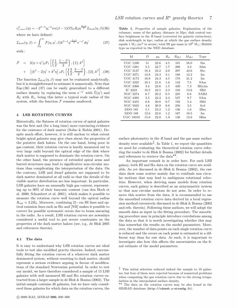
Table 1. Properties of sample galaxies. Explanation of thecolumns : name of the galaxy, distance in Mpc; disk central sur-face brightness in the R band (corrected for galactic extinction);disk scalelength in kpc; radius at which the gas surface densityequals 1 M⊙/pc2 in arcsec; total HI gas mass in 108 M⊙; Hubbletype as reported in the NED database.

Id D µ0 Rd RHI MHI Type

UGC 1230 51 22.6 4.5 101 58.0 SmUGC 1281 5.5 22.7 1.7 206 3.2 SdmUGC 3137 18.4 23.2 2.0 297 43.6 SbcUGC 3371 12.8 23.3 3.1 188 12.2 ImUGC 4173 16.8 24.3 4.5 178 21.2 ImUGC 4325 10.1 21.6 1.6 142 7.5 SAmNGC 2366 3.4 22.6 1.5 439 7.3 IB(s)mIC 2233 10.5 22.5 2.3 193 13.6 SBd

NGC 3274 6.7 20.2 0.5 225 6.6 SABdNGC 4395 3.5 22.2 2.3 527 9.7 SAmNGC 4455 6.8 20.8 0.7 192 5.4 SBdNGC 5023 4.8 20.9 0.8 256 3.5 ScdDDO 185 5.1 23.2 1.2 136 1.6 IBmDDO 189 12.6 22.6 1.2 167 10.5 Im

UGC 10310 15.6 22.0 1.9 130 12.6 SBm

surface photometry in the R band and the gas mass surface

density were available‖. In Table 1, we report the quantitieswe need for evaluating the theoretical rotation curve refer-ring the reader to de Blok & Bosma (2002) for further detailsand references to retrieve the data⋆⋆.

An important remark in in order here. For each LSBgalaxy, both HI and Hα data on the rotation curve are avail-able. As yet discussed in de Blok & Bosma (2002), the rawdata show some scatter mainly due to residuals non circu-lar motions that may lead to ambiguous rotational veloc-ities. However, when deriving mass models from rotationcurves, each galaxy is described as an axisymmetric systemso that non circular motions do not arise. In order to re-move this scatter from the data, it is recommended to usethe smoothed rotation curve data derived by a local regres-sion method extensively discussed in de Blok & Bosma (2002and refs. therein). Following these authors, we will adopt thesmooth data as input in the fitting procedure. The smooth-ing procedure may in principle introduce correlations amongthe data so that it is worth investigating whether this maybias somewhat the results on the model parameters. More-over, the number of data points on each single rotation curveis reduced and the errors on each point is estimated in a dif-ferent way than for raw data. As such, it is important toinvestigate also how this affects the uncertainties on the fi-nal estimate of the model parameters.

‖ This initial selection reduced indeed the sample to 19 galax-ies, but four of them were rejected because of numerical problemswhen computing the gas rotation curve due to the strong irregu-larities in the interpolated surface density.⋆⋆ The data on the rotation curves may be also found in theSIMBAD database (http://cdsweb.u-strasbg.fr).

c© 0000 RAS, MNRAS 000, 000–000


4.2 Modelling LSB galaxies

Since we are interested in fitting rotation curves withoutany dark matter halo, our model for a generic LSB galaxyis made out of the stellar and gaseous components only.

We assume the stars are distributed in an infinitely thinand circularly symmetric disk. The surface density Σ(R)may be derived from the surface brightness distribution :

µ(R) = −2.5 log I(R)

with I(R) = Σ(R)/Υ⋆ the light distribution and Υ⋆ the stel-lar mass - to - light (hereafter M/L) ratio. The photometricdata (in the R band) are fitted with an exponential modelthus allowing to determine the scalelength Rd and the cen-tral surface brightness µ0 and hence I0 = I(R = 0). Theonly unknown parameter is therefore Υ⋆ that makes it pos-sible to convert the central luminosity density I0 into thecentral surface mass density Σ0 entering Eqs.(35) and (36).

Modelling the gas distribution is quite complicated. Fol-lowing the standard practice, we assume the gas is dis-tributed in a infinitely thin and circularly symmetric diskassuming for the surface density Σ(R) the profile that hasbeen measured by the HI 21 - cm lines. Since the measure-ments only cover the range Rmin ≤ R ≤ Rmax, we use athird order interpolation for R in this range, a linear extrap-olation between Rmax and RHI , being this latter a scalingradius defined by Σ(RHI) = 1 M⊙/pc

2, while we assumeΣ(R) = Σ(Rmin) for R ≤ Rmin. To check if the modelworks correctly, we compute the total mass MHI and nor-malize the model in such a way that this value is the sameas that is measured by the total HI 21 - cm emission. Finally,we increase the surface mass density by 1.4 to take into ac-count the helium contribution. It is worth noting that ourmodel is only a crude approximation for R outside the range(Rmin, Rmax), while, even in the range (Rmin, Rmax), Σ(R)gives only an approximated description of the gas distribu-tion since this latter may be quite clumpy and thereforecannot be properly fitted by any analytical expression. Westress, however, that the details of the gas distribution arerather unimportant since the rotation curve is dominatedeverywhere by the stellar disk. The clumpiness of the gasdistribution manifests itself in irregularities in the rotationcurve that may be easily masked in the fitting procedure,even if this is not strictly needed for our aims.

4.3 Fitting the rotation curve

Having modelled a LSB galaxy, Eqs.(35) – (38) may bestraightforwardly used to estimate the theoretical rotationcurve as function of three unknown quantities, namely thestellar M/L ratio Υ⋆ and the two theory parameters (β, rc).Actually, we will consider as fitting parameters log rc ratherthan rc (in kpc) since this is a more manageable quantitythat makes it possible to explore a larger range for this theo-retically unconstrained parameter. Moreover, we use the gasmass fraction fg rather than Υ⋆ as fitting quantity since therange for fg is clearly defined, while this is not for Υ⋆. Thetwo quantities are easily related as follows :

fg =Mg

Mg +Md⇐⇒ Υ⋆ =

(1− fg)Mg

fgLd(39)

with Mg = 1.4MHI the gas (HI + He) mass, Md = Υ⋆Ld

and Ld = 2πI0R2d the disk total mass and luminosity.

We use Eq.(35) to compute the disk Newtonian rotationcurve, while the vc,corr is obtained by integrating numeri-cally Eq.(37). For the gas, instead, we resort to numericalintegrations for both the Newtonian rotation curve and thecorrective term. The total rotation curve is finally obtainedby adding in quadrature these contributions.

To constrain the parameters (β, log rc, fg), we minimizethe following merit function :

χ2(p) =

N∑

i=1

[

vc,th(ri)− vc,obs(ri)

σi

]2

(40)

where the sum is over theN observed points. While using thesmoothed data helps in better adjusting the theoretical andobserved rotation curves, the smoothing procedure impliesthat the errors σi on each point are not Gaussian distributedsince they also take into account systematic misalignmentsbetween HI and Hα measurements and other effects leadingto a conservative overestimate of the true uncertainties (seethe discussion in (de Blok & Bosma 2002) for further de-tails). As a consequence, we do not expect that χ2/dof ≃ 1for the best fit model (with dof = N − 3 the number of de-grees of freedom), but we can still compare different modelson the basis of the χ2 values. In particular, the uncertain-ties on the model parameters will be estimated exploring thecontours of equal ∆χ2 = χ2 −χ2

min in the parameter space.

5 TESTING THE METHOD

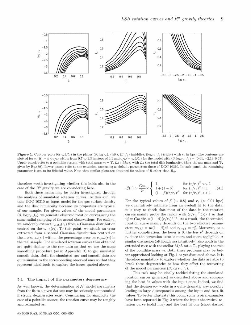
The method we have outlined above and the data on LSBgalaxies are in principle all what we need to test the viabilityof Rn gravity. However, there are some subtle issues that canaffect in an unpredictable way the outcome of the analysis.

Two main problems worth to be addressed. First, thereare three parameters to be constrained, namely the gas massfraction fg (related to the stellar M/L ratio Υ⋆) and the Rn

gravity quantities (β, log rc). However, although they do notaffect the theoretical rotation curve in the same way, thereare still some remaining degeneracies hard to be broken.This problem is well illustrated by Fig.,1 where we showthe contours of equal vc(Rd) in the planes (β, log rc), (β, fg)and (log rc, fg) for the pointlike and extended case. Looking,for instance, at right panels, one sees that, for a given β,log rc and fg (and hence Υ⋆) have the same net effect onthe rotation curve so that the same value for vc(Rd) maybe obtained for a lower fg provided one increases log rc. Onthe other hand, β and log rc have opposite effects on vc(R) :the lower is β, the smaller is vc(R) for a given R. Sincethe opposite holds for log rc, as a result, the same value ofvc(Rd) may be obtained increasing log rc and decreasing β.Moreover, while β drives the shape of the rotation curve inthe outer region, its effect may be better appreciated if rc islow so that a further degeneracy arises.

A second issue is related to our decision to use thesmooth rather than the raw data. Although de Blok &Bosma (2002) claim that this does not affect the results,their analysis is nevertheless performed in the framework ofstandard theory of gravity with dark matter haloes. It is

c© 0000 RAS, MNRAS 000, 000–000


0.2 0.4 0.6 0.8β

-3.5

-3

-2.5

-2

-1.5

-1

-0.5

log

r c

0.2 0.4 0.6 0.8β

0.2

0.4

0.6

0.8f g

-3.5 -3 -2.5 -2 -1.5 -1 -0.5log r c

0.2

0.4

0.6

0.8

f g

0.2 0.4 0.6 0.8β

-3.5

-3

-2.5

-2

-1.5

-1

-0.5lo

gr c

0.2 0.4 0.6 0.8β

0.2

0.4

0.6

0.8

f g

-3.5 -3 -2.5 -2 -1.5 -1 -0.5log r c

0.2

0.4

0.6

0.8

f gFigure 1. Contour plots for vc(Rd) in the planes (β, log rc), (left), (β, fg) (middle), (log rc, fg) (right) with rc in kpc. The contours areplotted for vc(R) = k×vfid with k from 0.7 to 1.3 in steps of 0.1 and vfid = vc(Rd) for the model with (β, log rc, fg) = (0.61,−2.13, 0.65).Upper panels refer to a pointlike system with total mass m = Υ⋆Ld+MHI , with Ld the total disk luminosity, MHI the gas mass and Υ⋆

given by Eq.(39). Lower panels refer to the extended case using as default parameters those of UGC 10310. In each panel, the remainingparameter is set to its fiducial value. Note that similar plots are obtained for values of R other than Rd.

therefore worth investigating whether this holds also in thecase of the Rn gravity we are considering here.

Both these issues may be better investigated throughthe analysis of simulated rotation curves. To this aim, wetake UGC 10310 as input model for the gas surface densityand the disk luminosity because its properties are typicalof our sample. For given values of the model parameters(β, log rc, fg), we generate observed rotation curves using thesame radial sampling of the actual observations. For each ri,we randomly extract vc,obs(ri) from a Gaussian distributioncentred on the vc,th(ri). To this point, we attach an errorextracted from a second Gaussian distribution centred onthe εi×vc,obs(ri) with εi the percentage error on vc,obs(ri) inthe real sample. The simulated rotation curves thus obtainedare quite similar to the raw data so that we use the samesmoothing procedure (as in Appendix B) to get simulatedsmooth data. Both the simulated raw and smooth data arequite similar to the corresponding observed ones so that theyrepresent ideal tools to explore the issues quoted above.

5.1 The impact of the parameters degeneracy

As well known, the determination of N model parametersfrom the fit to a given dataset may be seriously compromisedif strong degeneracies exist. Considering for simplicity thecase of a pointlike source, the rotation curve may be roughlyapproximated as :

v2c (r) ≃Gm

2r×

1 for (r/rc)β << 1

1 + (1− β) for (r/rc)β ≃ 1

(1− β)(r/rc)β for (r/rc)

β >> 1

.(41)

For the typical values of β (∼ 0.8) and rc (≃ 0.01 kpc)we qualitatively estimate from an eyeball fit to the data,it is easy to check that most of the data in the rotationcurves mainly probe the region with (r/rc)

β >> 1 so thatv2c ≃ Gm/2rc×(1−β)(r/rc)

β−1. As a result, the theoreticalrotation curve mainly depends on the two effective param-eters meff = m(1 − β)/2 and rc,eff = rβc . Moreover, as afurther complication, the lower is β, the less v2c depends onrc since the correction term is more and more negligible. Asimilar discussion (although less intuitively) also holds in theextended case with the stellar M/L ratio Υ⋆ playing the roleof the pointlike mass m. Both these problems may be bet-ter appreciated looking at Fig. 1 as yet discussed above. It istherefore mandatory to explore whether the data are able tobreak these degeneracies or how they affect the recoveringof the model parameters (β, log rc, fg).

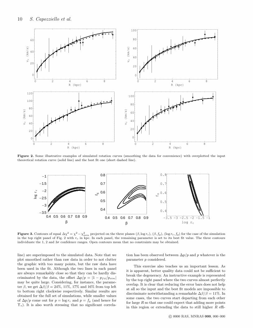
This task may be ideally tackled fitting the simulatedrotation curves generated as described above and compar-ing the best fit values with the input ones. Indeed, we findthat the degeneracy works in a quite dramatic way possiblyleading to large discrepancies among the input and best fitvalues. To better illustrate this point, some typical exampleshave been reported in Fig. 2 where the input theoretical ro-tation curve (solid line) and the best fit one (short dashed

c© 0000 RAS, MNRAS 000, 000–000


0 2 4 6 8R HkpcL

0

20

40

60

vcHkmsL

0 2 4 6 8R HkpcL

0

20

40

60

80

100

vcHkmsL

0 2 4 6 8R HkpcL

0

20

40

60

80

100

120

vcHkmsL

0 2 4 6 8R HkpcL

0

20

40

60

80

100

vcHkmsL

Figure 2. Some illustrative examples of simulated rotation curves (smoothing the data for convenience) with overplotted the inputtheoretical rotation curve (solid line) and the best fit one (short dashed line).

0.4 0.5 0.6 0.7 0.8 0.9β

-3.5

-3

-2.5

-2

-1.5

-1

log

r c

0.4 0.5 0.6 0.7 0.8 0.9β

0.4

0.5

0.6

0.7

0.8

f g

-3.5 -3 -2.5 -2 -1.5 -1log rc

0.4

0.5

0.6

0.7

0.8

fg

Figure 3. Contours of equal ∆χ2 = χ2−χ2min projected on the three planes (β, log rc), (β, fg), (log rc, fg) for the case of the simulation

in the top right panel of Fig. 2 with rc in kpc. In each panel, the remaining parameter is set to its best fit value. The three contoursindividuate the 1, 2 and 3σ confidence ranges. Open contours mean that no constraints may be obtained.

line) are superimposed to the simulated data. Note that weplot smoothed rather than raw data in order to not clutterthe graphic with too many points, but the raw data havebeen used in the fit. Although the two lines in each panelare always remarkably close so that they can be hardly dis-criminated by the data, the offset ∆p/p = |1 − pfit/psim|may be quite large. Considering, for instance, the parame-ter β, we get ∆β/β = 24%, 11%, 17% and 16% from top leftto bottom right clockwise respectively. Similar results areobtained for the full set of simulations, while smaller valuesof ∆p/p come out for p = log rc and p = fg (and hence forΥ⋆). It is also worth stressing that no significant correla-

tion has been observed between ∆p/p and p whatever is theparameter p considered.

This exercise also teaches us an important lesson. Asit is apparent, better quality data could not be sufficient tobreak the degeneracy. An instructive example is representedby the top right panel where the two curves almost perfectlyoverlap. It is clear that reducing the error bars does not helpat all so the input and the best fit models are impossible todiscriminate notwithstanding a remarkable ∆β/β = 11%. Insome cases, the two curves start departing from each otherfor large R so that one could expect that adding more pointsin this region or extending the data to still higher R effi-

c© 0000 RAS, MNRAS 000, 000–000


ciently breaks the degeneracy. Unfortunately, the simulateddata extend up to ∼ 5Rd so that further increasing thiscoverage with real data is somewhat unrealistic (especiallyusing typical spiral galaxies rather than the gas rich LSBs).

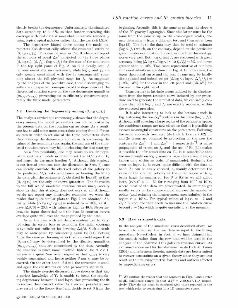
The degeneracy hinted above among the model pa-rameters also dramatically affects the estimated errors on(β, log rc, fg). This can be seen in Fig. 3 where we reportthe contours of equal ∆χ2 projected on the three planes(β, log rc), (β, fg), (log rc, fg) for the case of the simulationin the top right panel of Fig. 2. As it is clearly seen, βremains essentially unconstrained, while log rc and fg areonly weakly constrained with the 3σ contours still span-ning almost the full physical range for fg. As suggestedby the analysis of the pointlike case, these discouraging re-sults are an expected consequence of the dependence of thetheoretical rotation curve on the two degenerate quantities(meff , rc,eff ) preventing us to efficiently constraint sepa-rately the three model parameters.

5.2 Breaking the degeneracy among (β, log rc, fg)

The analysis carried out convincingly shows that the degen-eracy among the model parameters can not be broken bythe present data on the rotation curves alone. As a result,one has to add some more constraints coming from differentsources in order to set one of the three parameters abovethus breaking the degeneracy and correctly recovering thevalues of the remaining two. Again, the analysis of the simu-lated rotation curves may help in choosing the best strategy.

As a first possibility, one may resort to stellar popu-lation synthesis models in order to set the M/L ratio Υ⋆

and hence the gas mass fraction fg. Although this strategyis not free of problems (see the discussion in Sect. 6), onecan ideally correlate the observed colors of the galaxy tothe predicted M/L ratio and hence performing the fit tothe data with the parameter fg obtained by Eq.(39) so that(β, log rc) are the only unknown quantities. The fit resultsto the full set of simulated rotation curves unequivocallyshow us that this strategy does not work at all. Althoughwe do not report any illustrative examples, we warn thereader that quite similar plots to Fig. 2 are obtained. Ac-tually, while |∆ log rc/ log rc| is reduced to ∼ 10%, we stillhave |∆β/β| ∼ 20% with values as high as 40%. Neverthe-less, the input theoretical and the best fit rotation curvesoverlaps quite well over the range probed by the data.

As in the case with all the parameters free to vary,reducing the errors bars or extending the radial coverageis typically not sufficient for lowering ∆β/β. Such a resultmay be anticipated by considering again Eq.(41). SettingΥ⋆ is the same as choosing m so that one could argue that(β, log rc) may be determined by the effective quantities(meff , rc,eff ) that are constrained by the data. Actually,the situation is much more involved. Indeed, for β << 1,we are in a quasi Newtonian regime so that rc,eff is veryweakly constrained and hence neither β nor rc may be re-covered. On the other hand, if β ≃ 1 the correction is smalland again the constraints on both parameters are weak.

The simple exercise discussed above shows us that alsoa perfect knowledge of Υ⋆ is unable to break the remain-ing degeneracy between β and log rc thus preventing the fitto recover their correct value. As a second possibility, onemay resort to the theory itself and decide to set β from the

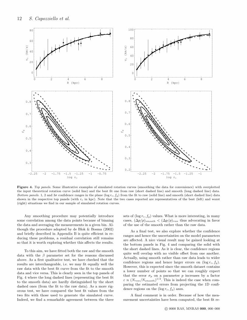
beginning. Actually, this is the same as setting the slope nof the Rn gravity Lagrangian. Since this latter must be thesame from the galactic up to the cosmological scales, onemay determine n from a different test and then set β fromEq.(15). The fit to the data may then be used to estimate(log rc, fg) which, on the contrary, depend on the particularsystem under examination. Indeed, we find that this strategyworks very well. Both log rc and fg are recovered with greataccuracy being |∆ log rc/ log rc| ∼ |∆fg/fg | ∼ 5% and nevergreater than ∼ 10%. Two cases representative of our bestand worst situations are shown in Fig. 4. In both cases, theinput theoretical curve and the best fit one may be hardlydistinguished and indeed we get (∆ log rc/ log rc,∆fg/fg) =(−2%,−3%) for the case in the left panel and (3%, 5%) forthe one in the right panel.

Considering the intrinsic errors induced by the displace-ment from the input rotation curve induced by our proce-dure used to generate the simulated data, we can safely con-clude that both log rc and fg are exactly recovered withinthe expected precision.

It is also interesting to look at the bottom panels inFig. 4 showing the iso -∆χ2 contours in the plane (log rc, fg).Although still covering a large region of the parameter space,the confidence ranges are now closed so that it is possible toextract meaningful constraints on the parameters. Followingthe usual approach (see, e.g., (de Blok & Bosma 2002)), 1and 2σ errors are obtained by projecting on the axes the

contours for ∆χ2 = 1 and ∆χ2 = 4 respectively††. A naivepropagation of errors on fg and the use of Eq.(39) makesit possible to infer constraints on Υ⋆. It is remarkable thatthe uncertainty on log rc remains large (hence rendering rcknown only within an order of magnitude). Reducing theerror on log rc is, however, quite difficult with the data athand. As can be easily checked, rc mainly determines thevalue of the circular velocity in the outer region with vcbeing larger for smaller rc. For β ≃ 0.8 as we will adoptlater, (r/rc)

β ≃ 1 − 50 for r ranging from 10−2 to 102rcwhere most of the data are concentrated. In order to getsmaller errors on log rc, one should increase the number ofpoints (and reducing the measurement uncertainties) in theregion r > 103rc. For typical values of log rc ≃ −2 andRd ≃ 2 kpc, one then needs to measure the rotation curvebeyond r ∼ 5Rd which is quite unrealistic at the moment.

5.3 Raw vs smooth data

In the analysis of the simulated cases described above, wehave up to now used the raw data as input to the fittingprocedure. Nevertheless, in Sect. 4, we have claimed thatthe smooth rather than the raw data will be used in theanalysis of the observed LSB galaxies rotation curves. Asexplained above and further discussed in de Blok & Bosma(2002) and references therein, smooth data are better suitedto recover constraints on a given theory since they are lesssensitive to non axisymmetric features and outliers affectedby unpredictable errors.

†† We caution the reader that the contours in Figs. 3 and 4 referto 2D confidence ranges so that ∆χ2 = 2.30, 6.17, 11.8 respec-tively. They do not must be confused with those reported in thetext which refer to constraints in a 1D parameter space.

c© 0000 RAS, MNRAS 000, 000–000


0 2 4 6 8R HkpcL

0

20

40

60

80vcHkmsL

0 2 4 6 8R HkpcL

0

20

40

60

80

100

vcHkmsL

-2.25 -2 -1.75 -1.5 -1.25 -1 -0.75log rc

0.3

0.4

0.5

0.6

0.7

0.8

fg

-2.25 -2 -1.75 -1.5 -1.25 -1log rc

0.2

0.3

0.4

0.5

0.6

0.7

0.8

fg

Figure 4. Top panels. Some illustrative examples of simulated rotation curves (smoothing the data for convenience) with overplottedthe input theoretical rotation curve (solid line) and the best fit one from raw (short dashed line) and smooth (long dashed line) data.Bottom panels. 1, 2 and 3σ confidence ranges in the plane (log rc, fg) from the fit to raw (solid line) and smooth (short dashed line) datashown in the respective top panels (with rc in kpc). Note that the two cases reported are representatives of the best (left) and worst(right) situations we find in our sample of simulated rotation curves.

Any smoothing procedure may potentially introducesome correlation among the data points because of binningthe data and averaging the measurements in a given bin. Al-though the procedure adopted by de Blok & Bosma (2002)and briefly described in Appendix B is quite efficient in re-ducing these problems, a residual correlation still remainsso that it is worth exploring whether this affects the results.

To this aim, we have fitted both the raw and the smoothdata with the β parameter set for the reasons discussedabove. As a first qualitative test, we have checked that theresults are interchangeable, i.e. we may fit equally well theraw data with the best fit curve from the fit to the smoothdata and vice versa. This is clearly seen in the top panels ofFig. 4 where the long dashed lines (representing the best fitto the smooth data) are hardly distinguished by the shortdashed ones (from the fit to the raw data). As a more rig-orous test, we have compared the best fit values from thetwo fits with those used to generate the simulated curve.Indeed, we find a remarkable agreement between the three

sets of (log rc, fg) values. What is more interesting, in manycases, (∆p/p)smooth < (∆p/p)raw thus advocating in favorof the use of the smooth rather than the raw data.

As a final test, we also explore whether the confidenceranges and hence the uncertainties on the model parametersare affected. A nice visual result may be gained looking atthe bottom panels in Fig. 4 and comparing the solid withthe short dashed lines. As it is clear, the confidence regionsquite well overlap with no visible offset from one another.Actually, using smooth rather than raw data leads to widerconfidence regions and hence larger errors on (log rc, fg).However, this is expected since the smooth dataset containsa lower number of points so that we can roughly expectthat the error σp on a parameter p increases by a factorε ∝ (Nraw/Nsmooth)

1/2. This is indeed the case when com-paring the estimated errors from projecting the 1D confi-dence regions on the (log rc, fg) axes.

A final comment is in order. Because of how the mea-surement uncertainties have been computed, the best fit re-

c© 0000 RAS, MNRAS 000, 000–000


duced χ2/d.o.f values are not expected to be close to 1.This is indeed the case when dealing with the raw data.However, a further reduction is expected for the smoothdata because of the peculiarities of the smoothing proce-dure used. For instance, we get (χ2/d.o.f.)raw = 0.29 vs(χ2/d.o.f.)smooth = 0.07 for the case in the right panel ofFig. 4. There are two motivations concurring to the find-ing of such small reduced χ2. First, the uncertainties havebeen conservatively estimated so that the true ones mayalso be significantly smaller. Should this be indeed the case,χ2/d.o.f. turn out to be underestimated. A second issuecomes from an intrinsic feature of the smoothing procedure.As discussed in Appendix B, the method we employ is de-signed to recover the best approximation of an underlyingmodel by a set of sparse data. Since the fit to the smoothdata searches for the best agreement between the model andthe data, an obvious consequence is that the best fit mustbe as close as possible to data that are by their own as closeas possible to the model. As such, if the best fit model re-produces the data, the χ2 is forced to be very small henceoriginating the observed very small values of the reducedχ2. Note that both these effects are systematics so that theywork the same way over the full parameters space. Since weare interested in ∆χ2 rather than χ2

min, these systematicscancel out thus not affecting anyway the estimate of theuncertainties on the model parameters.

6 RESULTS

The extensive analysis of the previous section make it possi-ble to draw two summarizing conclusions. First, we have toset somewhat the slope n of the gravity Lagrangian in orderto break the degeneracy the model parameters. Second, wecan rely on the smoothed data without introducing any biasin the estimated parameters or on their uncertainties.

A key role is then played by how we set n and hence β.To this aim, one may resort to cosmology. Indeed, Rn grav-ity has been introduced as a possible way to explain the ob-served cosmic speed up without the need of any dark energycomponent. Motivated by the first encouraging results, wehave fitted the SNeIa Hubble diagram with a model compris-ing only baryonic matter, but regulated by modified Fried-mann equations derived from the Rn gravity Lagrangian.Indeed, we find that the data are consistent with the hy-pothesis of no dark energy and dark matter provided n 6= 1is assumed (Capozziello, Cardone and Troisi 2006). Unfor-tunately, the constraints on n are quite weak so that we havedecided to set n to its best fit value without considering thelarge error. This gives β = 0.817 that we will use throughoutthe rest of the paper. Note that Eq.(15) quickly saturatesas function of n so that, even if n is weakly constrained, βturns out to be less affected.

A comment is in order here. Setting β to the value de-rived from data probing cosmological scales, we are implic-itly assuming that the slope n of the gravity Lagrangian isthe same on all scales. From a theoretical point of view, thisis an obvious consistency assumption. However, it shouldbe nicer to derive this result from the analysis of the LSBrotation curves since they probe a different scale. Unfortu-nately, the parameters degeneracy discussed above preventsus to efficiently perform this quite interesting test. Indeed,

an accurate estimate of n from β needs a well determined βsince a small offset ∆β/β translates in a dramatically large∆n/n. As a consequence, a possible inconsistency amongthe estimated β from different galaxies could erroneouslylead to the conclusion that the gravity theory is theoreticallynot self consistent. To validate such a conclusion, however,one should reduce ∆β/β to less than 5%. Unfortunately,our analysis of the simulated rotation curves have shown usthat this is not possible with the data at hand. It is there-fore wiser to opt for a more conservative strategy and look

for a consistency‡‡ between the results from the cosmologi-cal and the galactic scales exploring whether the value of βset above allows to fit all the rotation curves with physicalvalues of the remaining two parameters (log rc, fg). This isour aim in this paper, while the more ambitious task hintedabove will need for a different dataset.

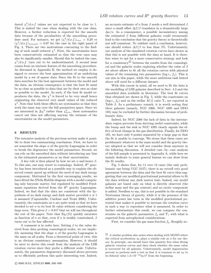
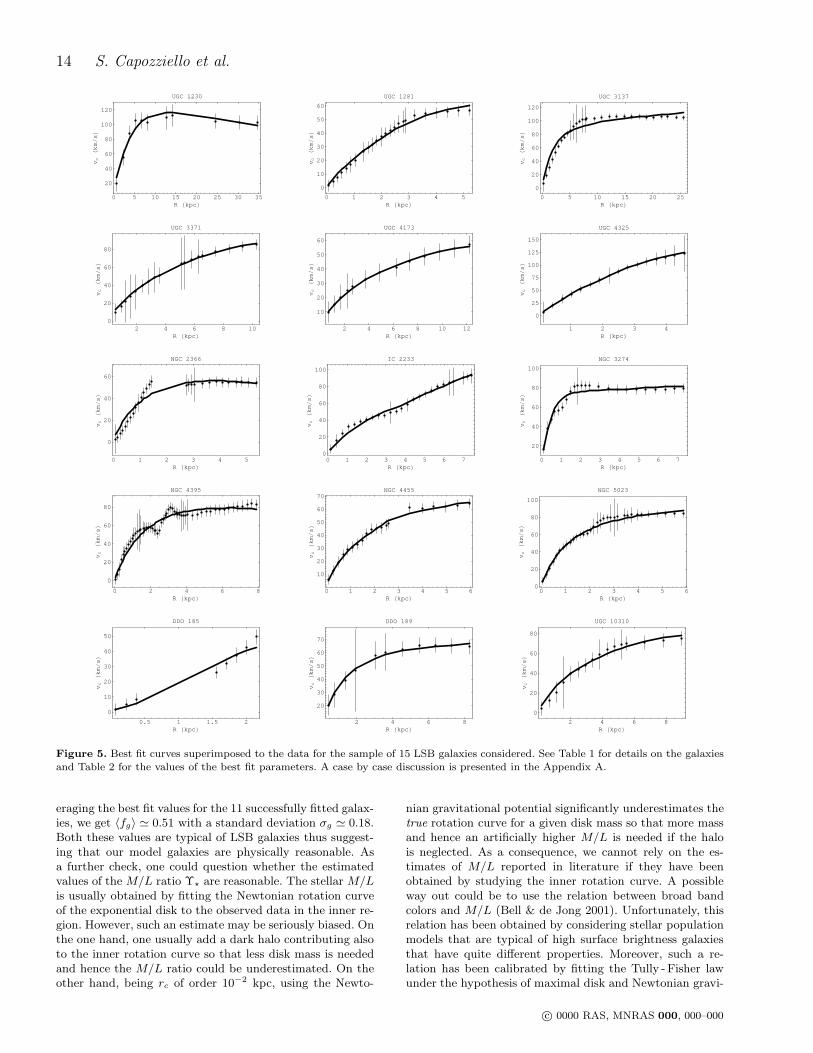
With this caveat in mind, all we need to fit the data isthe modelling of LSB galaxies described in Sect. 4.3 and thesmoothed data available in literature. The best fit curvesthus obtained are shown in Fig. 5, while the constraints on(log rc, fg) and on the stellar M/L ratio Υ⋆ are reported inTable 2. As a preliminary remark, it is worth noting thatthree galaxies (namely, NGC 2366, NGC 4395 and DDO185) may be excluded by further discussion because of prob-lematic data.

Indeed, for NGC 2366 the lack of data in the interme-diate region prevents from deriving useful constraints, whilethe bump and the sink in NGC 4395 clearly signals the ef-fect of local clumps in the gas distribution. Finally, for DDO185, we have only 8 points separated by a large gap so thatthe fit is unable to converge. We stress that these cases areproblematic whatever is the mass model and the gravity the-ory adopted so that we will not consider them anymore inthe following discussion. A detailed case - by - case analysisof the full sample is presented in Appendix A, while here wemainly dedicate to some general lessons we can draw fromthe fit results.

Fig. 5 shows that, for 11 over 12 cases (the only prob-lematic one being UGC 3137), there is an overall very goodagreement between the data and the best fit curve thus sug-gesting that our modified gravitational potential allows to fitthe data without any dark matter halo. Indeed, our modelgalaxies are based only on what is directly observed (thestellar mass and the gas content) and no exotic componentis added. Needless to say, this is not possible in the standardNewtonian theory of gravity, while it is the presence of theadditive power law term in the modified gravitational po-tential that makes it possible to increase the rotation curvein such a way to reproduce what is measured. In order tofurther substantiate this result, we can compare the con-straints on the galactic parameters fg and Υ⋆ with what isexpected from astrophysical considerations.

First, we consider the gas mass fraction fg . Roughly av-

‡‡ A similar problem also arises when dealing with MOND wherethe critical acceleration a0 plays a similar role as n for our the-ory. In principle, one should leave this quantity free when fittinggalactic rotation curves and then check whether the same valueis recovered for all galaxies. Unfortunately, model degeneraciesprevent to perform such a test so that it is common to set a0 toits fiducial value 1.2×10−10m/s2 from the beginning.

c© 0000 RAS, MNRAS 000, 000–000


0 5 10 15 20 25 30 35R HkpcL

20

40

60

80

100

120

vcHkmsL

UGC 1230

0 1 2 3 4 5R HkpcL

0

10

20

30

40

50

60

vcHkmsL

UGC 1281

0 5 10 15 20 25R HkpcL

0

20

40

60

80

100

120

vcHkmsL

UGC 3137

2 4 6 8 10R HkpcL

0

20

40

60

80

vcHkmsL

UGC 3371

2 4 6 8 10 12R HkpcL

10

20

30

40

50

60

vcHkmsL

UGC 4173

1 2 3 4R HkpcL

0

25

50

75

100

125

150

vcHkmsL

UGC 4325

0 1 2 3 4 5R HkpcL

0

20

40

60

vcHkmsL

NGC 2366

0 1 2 3 4 5 6 7R HkpcL

0

20

40

60

80

100

vcHkmsL

IC 2233

0 1 2 3 4 5 6 7R HkpcL

20

40

60

80

100

vcHkmsL

NGC 3274

0 2 4 6 8R HkpcL

0

20

40

60

80

vcHkmsL

NGC 4395

0 1 2 3 4 5 6R HkpcL

10

20

30

40

50

60

70

vcHkmsL

NGC 4455

0 1 2 3 4 5 6R HkpcL

0

20

40

60

80

100

vcHkmsL

NGC 5023

0.5 1 1.5 2R HkpcL

0

10

20

30

40

50

vcHkmsL

DDO 185

2 4 6 8R HkpcL

20

30

40

50

60

70

vcHkmsL

DDO 189

2 4 6 8R HkpcL

0

20

40

60

80

vcHkmsL

UGC 10310

Figure 5. Best fit curves superimposed to the data for the sample of 15 LSB galaxies considered. See Table 1 for details on the galaxiesand Table 2 for the values of the best fit parameters. A case by case discussion is presented in the Appendix A.

eraging the best fit values for the 11 successfully fitted galax-ies, we get 〈fg〉 ≃ 0.51 with a standard deviation σg ≃ 0.18.Both these values are typical of LSB galaxies thus suggest-ing that our model galaxies are physically reasonable. Asa further check, one could question whether the estimatedvalues of theM/L ratio Υ⋆ are reasonable. The stellar M/Lis usually obtained by fitting the Newtonian rotation curveof the exponential disk to the observed data in the inner re-gion. However, such an estimate may be seriously biased. Onthe one hand, one usually add a dark halo contributing alsoto the inner rotation curve so that less disk mass is neededand hence the M/L ratio could be underestimated. On theother hand, being rc of order 10−2 kpc, using the Newto-

nian gravitational potential significantly underestimates thetrue rotation curve for a given disk mass so that more massand hence an artificially higher M/L is needed if the halois neglected. As a consequence, we cannot rely on the es-timates of M/L reported in literature if they have beenobtained by studying the inner rotation curve. A possibleway out could be to use the relation between broad bandcolors and M/L (Bell & de Jong 2001). Unfortunately, thisrelation has been obtained by considering stellar populationmodels that are typical of high surface brightness galaxiesthat have quite different properties. Moreover, such a re-lation has been calibrated by fitting the Tully - Fisher lawunder the hypothesis of maximal disk and Newtonian gravi-

c© 0000 RAS, MNRAS 000, 000–000


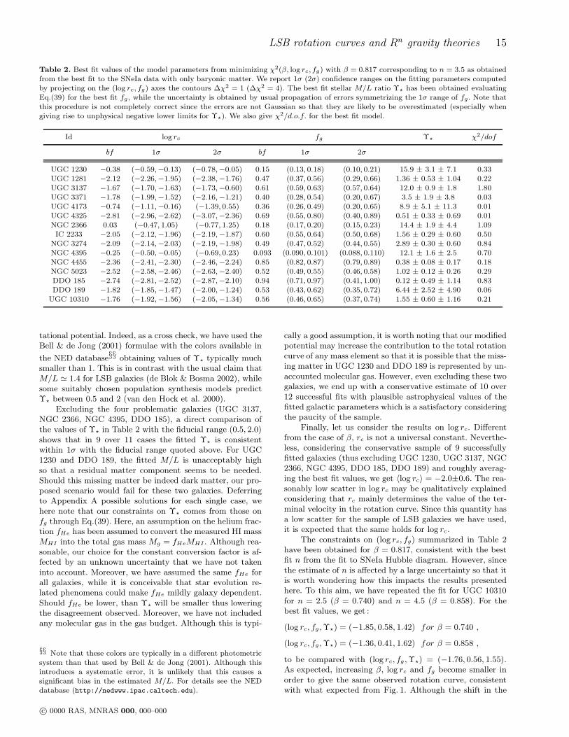
Table 2. Best fit values of the model parameters from minimizing χ2(β, log rc, fg) with β = 0.817 corresponding to n = 3.5 as obtainedfrom the best fit to the SNeIa data with only baryonic matter. We report 1σ (2σ) confidence ranges on the fitting parameters computedby projecting on the (log rc, fg) axes the contours ∆χ2 = 1 (∆χ2 = 4). The best fit stellar M/L ratio Υ⋆ has been obtained evaluatingEq.(39) for the best fit fg, while the uncertainty is obtained by usual propagation of errors symmetrizing the 1σ range of fg. Note thatthis procedure is not completely correct since the errors are not Gaussian so that they are likely to be overestimated (especially whengiving rise to unphysical negative lower limits for Υ⋆). We also give χ2/d.o.f. for the best fit model.

Id log rc fg Υ⋆ χ2/dof

bf 1σ 2σ bf 1σ 2σ

UGC 1230 −0.38 (−0.59,−0.13) (−0.78,−0.05) 0.15 (0.13, 0.18) (0.10, 0.21) 15.9 ± 3.1 ± 7.1 0.33UGC 1281 −2.12 (−2.26,−1.95) (−2.38,−1.76) 0.47 (0.37, 0.56) (0.29, 0.66) 1.36 ± 0.53 ± 1.04 0.22UGC 3137 −1.67 (−1.70,−1.63) (−1.73,−0.60) 0.61 (0.59, 0.63) (0.57, 0.64) 12.0 ± 0.9 ± 1.8 1.80UGC 3371 −1.78 (−1.99,−1.52) (−2.16,−1.21) 0.40 (0.28, 0.54) (0.20, 0.67) 3.5 ± 1.9 ± 3.8 0.03UGC 4173 −0.74 (−1.11,−0.16) (−1.39, 0.55) 0.36 (0.26, 0.49) (0.20, 0.65) 8.9 ± 5.1 ± 11.3 0.01UGC 4325 −2.81 (−2.96,−2.62) (−3.07,−2.36) 0.69 (0.55, 0.80) (0.40, 0.89) 0.51 ± 0.33 ± 0.69 0.01NGC 2366 0.03 (−0.47, 1.05) (−0.77, 1.25) 0.18 (0.17, 0.20) (0.15, 0.23) 14.4 ± 1.9 ± 4.4 1.09IC 2233 −2.05 (−2.12,−1.96) (−2.19,−1.87) 0.60 (0.55, 0.64) (0.50, 0.68) 1.56 ± 0.29 ± 0.60 0.50

NGC 3274 −2.09 (−2.14,−2.03) (−2.19,−1.98) 0.49 (0.47, 0.52) (0.44, 0.55) 2.89 ± 0.30 ± 0.60 0.84NGC 4395 −0.25 (−0.50,−0.05) (−0.69, 0.23) 0.093 (0.090, 0.101) (0.088, 0.110) 12.1 ± 1.6 ± 2.5 0.70NGC 4455 −2.36 (−2.41,−2.30) (−2.46,−2.24) 0.85 (0.82, 0.87) (0.79, 0.89) 0.38 ± 0.08 ± 0.17 0.18NGC 5023 −2.52 (−2.58,−2.46) (−2.63,−2.40) 0.52 (0.49, 0.55) (0.46, 0.58) 1.02 ± 0.12 ± 0.26 0.29DDO 185 −2.74 (−2.81,−2.52) (−2.87,−2.10) 0.94 (0.71, 0.97) (0.41, 1.00) 0.12 ± 0.49 ± 1.14 0.83DDO 189 −1.82 (−1.85,−1.47) (−2.00,−1.24) 0.53 (0.43, 0.62) (0.35, 0.72) 6.44 ± 2.52 ± 4.90 0.06

UGC 10310 −1.76 (−1.92,−1.56) (−2.05,−1.34) 0.56 (0.46, 0.65) (0.37, 0.74) 1.55 ± 0.60 ± 1.16 0.21

tational potential. Indeed, as a cross check, we have used theBell & de Jong (2001) formulae with the colors available in

the NED database§§ obtaining values of Υ⋆ typically muchsmaller than 1. This is in contrast with the usual claim thatM/L ≃ 1.4 for LSB galaxies (de Blok & Bosma 2002), whilesome suitably chosen population synthesis models predictΥ⋆ between 0.5 and 2 (van den Hock et al. 2000).

Excluding the four problematic galaxies (UGC 3137,NGC 2366, NGC 4395, DDO 185), a direct comparison ofthe values of Υ⋆ in Table 2 with the fiducial range (0.5, 2.0)shows that in 9 over 11 cases the fitted Υ⋆ is consistentwithin 1σ with the fiducial range quoted above. For UGC1230 and DDO 189, the fitted M/L is unacceptably highso that a residual matter component seems to be needed.Should this missing matter be indeed dark matter, our pro-posed scenario would fail for these two galaxies. Deferringto Appendix A possible solutions for each single case, wehere note that our constraints on Υ⋆ comes from those onfg through Eq.(39). Here, an assumption on the helium frac-tion fHe has been assumed to convert the measured HI massMHI into the total gas mass Mg = fHeMHI . Although rea-sonable, our choice for the constant conversion factor is af-fected by an unknown uncertainty that we have not takeninto account. Moreover, we have assumed the same fHe forall galaxies, while it is conceivable that star evolution re-lated phenomena could make fHe mildly galaxy dependent.Should fHe be lower, than Υ⋆ will be smaller thus loweringthe disagreement observed. Moreover, we have not includedany molecular gas in the gas budget. Although this is typi-

§§ Note that these colors are typically in a different photometricsystem than that used by Bell & de Jong (2001). Although thisintroduces a systematic error, it is unlikely that this causes asignificant bias in the estimated M/L. For details see the NEDdatabase (http://nedwww.ipac.caltech.edu).

cally a good assumption, it is worth noting that our modifiedpotential may increase the contribution to the total rotationcurve of any mass element so that it is possible that the miss-ing matter in UGC 1230 and DDO 189 is represented by un-accounted molecular gas. However, even excluding these twogalaxies, we end up with a conservative estimate of 10 over12 successful fits with plausible astrophysical values of thefitted galactic parameters which is a satisfactory consideringthe paucity of the sample.

Finally, let us consider the results on log rc. Differentfrom the case of β, rc is not a universal constant. Neverthe-less, considering the conservative sample of 9 successfullyfitted galaxies (thus excluding UGC 1230, UGC 3137, NGC2366, NGC 4395, DDO 185, DDO 189) and roughly averag-ing the best fit values, we get 〈log rc〉 = −2.0±0.6. The rea-sonably low scatter in log rc may be qualitatively explainedconsidering that rc mainly determines the value of the ter-minal velocity in the rotation curve. Since this quantity hasa low scatter for the sample of LSB galaxies we have used,it is expected that the same holds for log rc.

The constraints on (log rc, fg) summarized in Table 2have been obtained for β = 0.817, consistent with the bestfit n from the fit to SNeIa Hubble diagram. However, sincethe estimate of n is affected by a large uncertainty so that itis worth wondering how this impacts the results presentedhere. To this aim, we have repeated the fit for UGC 10310for n = 2.5 (β = 0.740) and n = 4.5 (β = 0.858). For thebest fit values, we get :

(log rc, fg ,Υ⋆) = (−1.85, 0.58, 1.42) for β = 0.740 ,

(log rc, fg ,Υ⋆) = (−1.36, 0.41, 1.62) for β = 0.858 ,

to be compared with (log rc, fg ,Υ⋆) = (−1.76, 0.56, 1.55).As expected, increasing β, log rc and fg become smaller inorder to give the same observed rotation curve, consistentwith what expected from Fig. 1. Although the shift in the

c© 0000 RAS, MNRAS 000, 000–000


best fit values is significant, the data do not still allow todraw a definitive conclusion. For instance, the 2σ confidenceranges for log rc turn out to be :

(−2.16,−1.39) for β = 0.740(−2.05,−1.34) for β = 0.817(−2.04,−1.35) for β = 0.858

(42)

which are consistent with each other. Note that further in-creasing n have no significant effect on the estimate of theparameters since β quickly saturates towards its asymptoticvalue β = 1. We are therefore confident that, although theconstraints on (log rc, β) depend on β, our main results arequalitatively unaltered by the choice of n (and hence β).

It is also worth noting that the three values of β con-sidered above all provide quite good fits to the observedrotation curve. This is not surprising given the data at handand our analysis parameters degeneracies presented in Sect.5. In order to constrain β from rotation curves leaving itas a free parameter in the fit, therefore, one could explorethe possibility to performed a combined χ2 analysis of thefull set of rotation curves. This can eventually be comple-mented by adding a prior on β, e.g., from the cosmologicalconstraints on n. Exploring this issue is outside our aimshere, but should be addressed in a forthcoming paper.

Summarizing, the results from the fit and the reason-able agreement between the recovered Υ⋆ and that predictedfrom stellar population synthesis models make us confidentthat Rn gravity is indeed a possible way to fit the rota-tion curves of LSB galaxies using only baryonic components(namely, the stellar disk and the interstellar gas) thus es-caping the need of any putative dark matter halo.

7 DISCUSSION AND CONCLUSIONS

Rotation curves of spiral galaxies have been consideredfor a long time the strongest evidence of the existence ofdark matter haloes surrounding their luminous components.Notwithstanding the great experimental efforts, up to nowthere has never been any firm detection of such an exoticdark component that should make up these haloes. It istherefore worth wondering whether dark matter indeed ex-ists or it is actually the signal of the need for a differentgravitational physics.

Motivated by these considerations, we have exploredhere the case of Rn gravity. Since such theories have beendemonstrated to be viable alternatives to the dark energygiving rise to scenarios capable of explaining the observedcosmic speed up, it is highly interesting to investigate theirconsequences also at galactic scales. To this aim, we havesolved the vacuum field equations for power - law f(R) the-ories in the low energy limit thus deriving the gravitationalpotential of a pointlike source. It turns out that both the po-tential and the rotation curve are corrected by an additiveterm scaling as (r/rc)

β−1 with the scalelength rc dependingon the system physical features (e.g. the mass) and β a func-tion of the slope n of the gravity Lagrangian. In particular,for n = 1, our approximated solution reduces to the stan-dard Newtonian one. For 0 < β < 1, the potential is stillasymptotically vanishing, but the rotation curve is higherthan the Newtonian one. These results still hold when wecompute the corrected potential for extended systems with

spherical symmetry or thin disk configuration. As a result,we have argued that the rotation curve of spiral galaxiescould be fitted using the luminous components only thuseliminating the need for dark matter.

In order to verify this hypothesis, we have considereda sample of 15 LSB galaxies with well measured combinedHI and Hα rotation curves extending far beyond the opticaledge of the disk. Since these systems are usually claimed tobe dark matter dominated, reproducing their rotation curveswithout the need of any dark matter halo would representa significant evidence in favour of Rn gravity. Moreover, fit-ting to rotation curves allows in principle to constrain thetheory parameters (β, rc) and determine the M/L ratio ofthe stellar component. Unfortunately, extensive simulationshave highlighted the need to set a strong prior on β (andhence n) to break the degeneracy among the three fittingparameters (β, log rc, fg). To this aim, we have resorted tothe results of SNeIAa Hubble diagram fitting without darkmatter and dark energy which shows that n = 3.5 repro-duces the data without the need of any dark sector.

Motivated by this consideration, we have set n = 3.5giving β = 0.817 in order to check whether Rn gravity mayfit both the SNeIa Hubble diagram and the LSB rotationcurves without either dark energy on cosmological scalesand dark matter on galactic scales with the same value ofthe slope n. Indeed, we conservatively estimate that 10 of asample of 12 usable galaxies can be properly fitted by thecorrected rotation curves based only on the baryonic com-ponents (stars and gas) of the galaxies with values of theM/L ratio which may be reconciled with predictions fromstellar population synthesis models. It is worth emphasiz-ing that all the LSB rotation curves have been successfullyfitted using the same value of β. Although β has been setfrom the beginning, this does not guarantee that the full setof curves will be satisfactorily well fitted. Indeed, should wehave found that a single rotation curve demands for a differ-ent β, this could have been a decisive evidence against Rn

gravity. On the contrary, the same β leads to equally goodfit for all the 10 successful galaxies. We therefore concludethat the self consistency of the theory has been verified thusleading further support to Rn gravity as a viable alternativeto the dark sector on galactic and cosmological scales.

These encouraging results are a strong motivation forinvestigating Rn gravity further from both observational andtheoretical point of views. Still remaining on galactic scales,it is mandatory to extend the analysis of the rotation curvesto the case of high surface brightness (HSB) galaxies. Al-though their structure is more complicated (since one hasto include also a bulge component), HSB galaxies are morenumerous than LSB ones so that we may perform our test ona larger sample thus increasing the significance of the results.To this aim, it is important to carefully select the sample inorder to include systems with well measured and extendedrotation curve and not affected by possible non circular mo-tions due to spiral arms or bar - like structures. While thiscould be a limitation, it is worth stressing that in modelingHSB one may neglect the gas component which has beenthe most important source of theoretical uncertainty in ourstudy of LSB galaxies. Should the test on HSB be successfulas the present one, we could convincingly demonstrate thatRn gravity is a no dark matter solution to the long standingproblem of the rotation curves of spiral galaxies.

c© 0000 RAS, MNRAS 000, 000–000


As well known, dark matter is invoked also on largerthan galactic scales. For instance, dark matter haloes aretypically present in clusters of galaxies and enter in a cru-cial way in determining the gas temperature profile which ismeasured from the X - ray emission. In such a case, the formof the gravitational potential plays a key role so that it isworth investigating whether our modified potential could re-produce the observed temperature profile without the needof dark matter. This test should also represent a furthercheck of the consistency of the theory since it allows a de-termination of β on a completely different scale. Of course,one should find the same β, while a significant differencecould be a clear signal of unescapable problems. Note thatthere are nowadays a large number of clusters whose gastemperature profiles is well measured thanks to the Chan-

dra and XMM-Newton satellites so that also this test couldbe performed on a large sample to ameliorate the statistics.

A step further leads us to the cosmological scales wheredark matter is introduced to fill the gap between the bary-onic density parameter Ωb and the estimated total matterone ΩM . According to nucleosynthesis predictions, Ωb =0.0214±0.0020 (Kirkman et al. 2003), while ΩM ≃ 0.25 isestimated by SNeIa Hubble diagram and matter power spec-trum. Such a large discrepancy may seem to be impossible tocure without resorting to dark matter. However, this couldalso not be the case when considering that both the SNeIaHubble diagram and the matter power spectrum are usuallycomputed assuming General Relativity as the correct theoryof gravity. However, should f(R) theories be indeed the cor-rect model, one should recompute ab initio the matter powerspectrum so that it is impossible to predict a priori what isthe value of ΩM that allows a nice fit to the measured matterpower spectrum in a higher order theory. There is thereforemuch room for further investigation and it is indeed possi-ble that a baryons only universe is in agreement with thecosmological data if an alternative theory of gravity, insteadof Einstein General Relativity, is used.

As a final comment, we would like to stress the powerof an approach based on higher order theories of gravity.Although it is still possible that the choice f(R) = f0R

n isunable to positively pass all the tests we have quoted above,it is important to note that f(R) theories are the uniquemechanism able to explain in a single theoretical frameworkphysical phenomena taking place on widely different scales.In our opinion, therefore, if a unified solution of the darkmatter and dark energy problems exist, this is the realmwhere it has to be searched for with the greatest chances ofsuccessful results.

Acknowledgements. We warmly thank M. Capaccioli forthe interesting discussions and encouragements. We are alsoextremely grateful to W.J.G. de Blok for his prompt an-swers to the many questions on the data and the LSB mod-eling, to G. D’Agostini for an illuminating discussion on theuse of marginalized likelihood functions and to F. Giubileofor help with data retrieving. We also thank G. Lambiase,C. Rubano and G. Scarpetta for discussions and commentson preliminary versions of the paper. Finally, the referee isgreatly acknowledged for his suggestions that have helpedto radically improve the paper.

APPENDIX A: DETAILS ON FIT RESULTS

In Sect. 6, we have discussed the main features of the fitresults as a whole, while here we give some few details onthe comparison of the model with the rotation curve on acase - by - case basis.

UGC 1230. This is a somewhat problematic case givinga best fit Υ⋆ = 15.9±3.1 which is hard to explain in termsof reasonable population synthesis models. High values ofM/L are also obtained in the case of maximum disk anddark halo models. For instance, de Blok & Bosma (2002) findΥ⋆ = 6.1 for both isothermal and NFW dark halo models. Itis therefore likely that a problem may reside in the data orin the modelling (e.g., an underestimate of the gas contentor a wrong measurement of the distance of the galaxy thatcould lead to underestimate the total absolute luminosityand hence overestimating Υ⋆). Although such a possibilityexist, it is worth noting that the value of log rc is signifi-cantly larger than what is found for the other galaxies thusenhancing the need for an unseen component at odds withour working hypothesis of no dark matter. We have there-fore decided to not consider UGC 1230 as a successful fitseven if there is a good agreement between the data and thebest fit curve.

UGC 1281. This is a typical case with the model nicelyreproducing the data and a value of Υ⋆ in agreement withpopulation synthesis models. There is only a marginal over-estimate of the rotation curve for R ≤ 1 kpc, but it is wellwithin the errors. To this aim, we remark that a slight over-estimate of the theoretical rotation curve for the innermostpoints is expected for all galaxies since we have artificiallyassumed the gas surface density is flat in this region whereno data are available. Should this not be the actual situa-tion, vc turns out to be slightly biased high.

UGC 3137. This case is not satisfactory for our ap-proach. Indeed, the reduced χ2 for the best fit model isanomalously high (∼ 2) essentially due to the theoreticalcurve being higher than the observed one for the innermostpoints and smaller in the intermediate region. Moreover, theestimated Υ⋆ = 12.0±1.9 is too large to be reconciled withpopulation synthesis models. The disagreement is hard toexplain given that the data seem to be of good quality andthe curve is quite smooth. It is, however, worth noting thatit is not possible to achieve a good fit also in the dark mat-ter case whatever is the halo model used (see, e.g., de Blok& Bosma 2002). It has to be remarked that UGC 3137 isan edge - on galaxy so that deriving a disk mass model fromthe surface brightness involves a series of assumptions thatcould have introduced some unpredictable systematic error.

UGC 3371. The agreement between the data andthe model is extremely good and the estimated values of(log rc, fg) are typical of the sample we have considered. Thebest fit Υ⋆ is somewhat larger than expected on the basis ofstellar population model, but the fiducial Υ⋆ = 1.4 typicallyused in dark matter fitting is only 1σ smaller. We can there-fore consider this fit successfull and physically reasonable.

c© 0000 RAS, MNRAS 000, 000–000


UGC 4173. Although the agreement between the dataand the best fit model is almost perfect, this case is some-what more problematic than UGC 3371 since we get ananomalously high Υ⋆. As such, we could deem this galaxyas a failure for Rn gravity. However, examining the 2D con-fidence regions in the plane (log rc, fg), it is easy to findout models with typical values of log rc and lower Υ⋆ thatcould still agree with the rotation curve within the errors.Moreover, the uncertainties on the data points are proba-bly overestimated as could be inferred noting that also darkhalo models reproduce the observed curve with a very smallχ2 which is a typical signal of too high errors. Given theseissues, we include this galaxy in the sample of successful fits.

UGC 4325. The best fit model matches perfectly theobserved rotation curve with a typical value of log rc, buta somewhat small but still reasonable Υ⋆. However, sincelog rc and Υ⋆ are positively correlated, one could increaselog rc and hence Υ⋆ still achieving a very good fit to thedata, even if this is not our final choice.

NGC 2366. This curve is a challenge both for Rn grav-ity and dark matter models. The very linear rise in the innerpart rapidly changes in a flat part at larger radii. Moreover,there are no points in the intermediate region that couldgive constraints on how the change takes place. As de Blok& Bosma (2002) suggests, it is possible that the outermostpoints which are based on the HI data alone are underes-timated. Another possibility is the presence of non circularmotions due to the inner bar - like structure. These uncer-tainties on the data lead to a very bad fit with large valuesfor both log rc and Υ⋆. Given this situation, we have notconsidered anymore this galaxy stressing, however, that thisis not an evidence against Rn gravity.

IC 2233. It is quite difficult to get a very good fit to thisgalaxy rotation curve since, looking at the plot, one sees anabrupt change of concavity for R ≥ 3 kpc. As a consequence,a perfect matching between the data and the model is notpossible. Nevertheless, the best fit model provides a quitegood agreement with the data. Moreover, the best fit valuesof (log rc, fg) are typical of our sample and the estimatedΥ⋆ nicely agrees with the fiducial one suggested in previousliterature. We can therefore consider this galaxy as one ofthe most remarkable successes of Rn gravity.

NGC 3274. Although the general trend of the curve iswell reproduced, there is a certain disagreement in the region1 kpc ≤ R ≤ 2 kpc where a change of concavity occurs thatis not reproduced by the model. Note that features like thiscould be related to a clumpiness in the gas distribution thatcannot be modeled analytically. Considering, moreover, thatthe value of log rc is quite typical and the estimated M/Lratio is not too difficult to reconcile with population synthe-sis models (although somewhat high), we conclude that Rn

gravity successfully reproduces this curve.

NGC 4395. The rotation curve of this galaxy is stronglyaffected by the presence of star formation regions that causean oscillating behaviour for 1.5 kpc ≤ R ≤ 4 kpc thatis not possible to reproduce by any analytical model. In-deed, the best fit model is unable to agree reasonably well

with the data so that the results on (log rc, fg) are signif-icantly altered. Given the problems with the modeling, wehave therefore decided to exclude this galaxy from the finalsample since it is impossible to decide whether a bad fit isa signal of a breakdown for Rn gravity.

NGC 4455. Both the fit and the estimated values of themodel parameters are quite satisfactory, although the lowΥ⋆ may argue in favour of a higher log rc. Note that thereis a hole in the observed rotation curve around ∼ 3 kpc.Adding some more data in this region could help in betterconstraining the parameters with particular regard to Υ⋆.It is worth noting that the best fit curve tends to be higher(but well within the measurement errors) in the outer region.Extending the measurement of this galaxy rotation curve tolarger radii could therefore be a crucial test for our paradigmin this particular case. Note, however, that it is also possiblethat the parameters will be adjusted in such a way to stillprovide a good fit.

NGC 5023. This edge - on galaxy is, in a certain sense,an ameliorated version of UGC 3137. Indeed, the best fitmodel underestimates the rotation curve in the region be-tween 2 and 3 kpc, but fits quite well the remaining data.Inspecting the rotation curve, a change of concavity occursat 2 kpc and it is, indeed, this feature the origin of the dis-agreement. The similarity with the case of UGC 3137 couldsuggest to reject this galaxy considering also this fit as anunsuccessful one. However, a closer look shows that, whilein the case of UGC 3137 the best fit model works bad bothin the inner and the intermediate regions, here the disagree-ment is limited to the zone where the change of concavitytakes place. Moreover, in this case, the best fit log rc is typi-cal of our sample and the estimated M/L ratio is quite rea-sonable so that we have finally decided to retain this galaxy.

DDO 185. This very linear curve is quite difficult to re-produce and, indeed, our best fit model makes a poor jobwith a too small M/L ratio. However, the overall rotationcurve measurements are of very poor quality so that thisgalaxy can be discarded from further considerations.

DDO 189. There is an almost perfect matching be-tween the data and the best fit model. The estimated val-ues of (log rc, fg) are typical for the LSB galaxies in oursample, but Υ⋆ is unexpectedly large. Since fg takes a com-pletely reasonable value, a possible problem could arise withthe conversion from fg to Υ⋆. For instance, should fHe besmaller than our fiducial value, then Υ⋆ should be revisedtowards lower values. In order to be conservative, we havehowever decided to exclude this galaxy from the sample ofsuccessful fits even if nothing prevents the reader to take theopposite decision.

UGC 10310. Everything works well for this galaxy. Thebest fit model provides a good fit to the observed rotationcurve with only a modest overestimate (still within the un-certainties) in the innermost region that could be ascribedto our assumptions in the gas modelling. The values of log rcand fg are typical of our sample, while the best fit Υ⋆ maybe easily reconciled with the predictions from stellar popu-lation synthesis models.

c© 0000 RAS, MNRAS 000, 000–000


APPENDIX B: SMOOTHING THE DATA

As input to the pipeline for testing Rn gravity, we haveused the smoothed version of the rotation curve data fol-lowing the same approach used by de Blok & Bosma (2002).As explained in Sect. 4, the use of the smooth rather thanthe raw data relies on the need to eliminate any residualeffect of non circular motions on the data since the gas anddisk mass models assume that these components are axisym-metric systems. However, the smoothing procedure may inprinciple introduce correlations among the data so that itis worth investigating whether this may bias somewhat theresults on the model parameters. This task has been ex-tensively performed in Sect. 5.3 so that here we only givesome more details on how the smoothing is done referringto Loader (1999) and de Blok & Bosma (2002) for furtherdetails.

First, the data have been symmetrized and folded andthen resampled each 6 arcsec. Since both HI and Hα dataare available, when there is an overlap, only Hα points havebeen retained for r ≤ rα with the values of rα available inTable 1 of de Blok & Bosma (2002). The smooth data havebeen obtained using a local regression method following thesteps schematically sketched below.

(i) Choose N points x1, . . . , xN .

(ii) Define the weight function w(u) = (1−|u|3)3 for |u| ≤1, w(u) = 0 for |u| > 1, with u = (x − xi)/h being h thewidth of the bin centred on xi.

(iii) Given a set of Nobs observed points (xj , vj), performa weighted fit of the polynomial Pp =

∑p

l=0al(x− xi)

l tothese data using the function w(u) defined above to generatethe weights.

(iv) Estimate the smoothed value of the rotation curve inxi as the zeroth order term of the polynomial fitted above.

(v) Repeat this procedure for each one of the N points(x1, . . . , xN) thus ending with a smoothed rotation curvedataset made out of N points (xi, vi).

It is worth stressing that this smoothing procedure intro-duces a negligible amount of correlations among the dif-ferent points in the rotation curve. Indeed, the fit of thepolynomial of degree p is performed only locally so that twoconsecutive bins have only a modest (if not null) number ofpoints in common depending on the chosen value of h. Asdiscussed in Loader (1999), local regression methods makeit possible to recover the information about a given functioneliminating the noise that affects the observed data. At thesame time, being local, the regression method minimizes thecorrelations between the different bins.

As shown in Sect. 5.3, the best fit model passes almostperfectly within the simulated smoothed data yielding a verysmall χ2 value. This is an expected consequence of the abil-ity of local regression methods to recover the true modelfrom noisy data. As such, if the fitted model reproduces thedata, it is, in a certain sense, forced to pass almost exactlythrough the smoothed points since they represent the bestapproximation to the true underlying model. If the fit issuccessful, the true model and the best fit model coincide sothat the χ2 is expected to be very small.

REFERENCES

Allemandi, G., Francaviglia, M., Ruggiero, M., Tartaglia, A. 2005,Gen. Rel. Grav., 37, 1891

Astier, P. et al. 2006, A&A, 447, 31

Bachall, N.A., Bode, P. 2003, ApJ, 588, 1

Bachall, N.A. et al. 2003, ApJ, 585, 182

Bell, E.F., de Jong, R.S. 2001, ApJ, 550, 212

Binney, J., Tremaine, S. 1987, Galactic dynamics, Princeton Uni-versity Books, Princeton (USA)

Borowiec, A., Godlowski, W., Szydlowski, M. 2006, Phys. Rev.

D, 74, 043502

Brodbeck, O., Straumann, N. 1993, J. Math. Phys., 34, 6

Bronnikov, K., Melnikov, V. 1994, Gen. Rel. Grav., 27, 465

Capozziello, S. 2002, Int. J. Mod. Phys. D, 11, 483

Capozziello, S., Cardone, V.F., Carloni, S., Troisi, A. 2003, Int.J. Mod. Phys. D, 12, 1969

Capozziello, S., Cardone, V.F., Carloni, S., Troisi, A. 2004, Phys.Lett. A, 326, 292

Capozziello, S., Cardone, V.F., Francaviglia, M. 2006, Gen. Rel.Grav., 38, 711

Capozziello, S., Cardone, V.F., Troisi, A. 2005, Phys. Rev. D, 71,043503

Capozziello, S., Cardone, V.F., Troisi, A. 2006, JCAP, 0608, 001

Capozziello, S., Carloni, S., Troisi, A. 2003, Rec. Res. Devel. As-tronomy. & Astrophys., 1, 625, astro - ph/0303041

Capozziello, S., Troisi, A. 2005, Phys. Rev. D, 72, 044022

Carloni, S., Dunsby, P.K.S., Capozziello, S., Troisi, A. 2005, Class.Quantum Grav. 22, 2839

Carroll, S.M., Duvvuri, V., Trodden, M., Turner, M.S. 2004, Phys.

Rev. D, 70, 043528

Carroll, S.M., Press, W.H., Turner, E.L. 1992, ARA&A, 30, 499

Catinella, B., Giovanelli, R., Haynes, M.P. 2006, ApJ, 640, 751

Cembranos, J.A.R. 2006, Phys. Rev. D, 73, 064029

Chiba, T. 2003, Phys. Lett. B, 575, 1

Clifton, T., Barrow, J.D. 2005, Phys. Rev. D, 72, 103005

Clocchiati, A. et al. 2006, APJ, 642, 1

Cole, S. et al. 2005, MNRAS, 362, 505

Croft, R.A.C., Hu, W., Dave, R. 1999, Phys. Rev. Lett., 83, 1092

de Bernardis, P. et al. 2000, Nature, 404, 955

de Blok, W.J.G., Bosma, A. 2002, A&A, 385, 816

de Blok, W.J.G. 2005, ApJ, 634, 227

Dick, R. 2004, Gen. Rel. Grav., 36, 217

Dolgov, A.D., Kawasaki, M. 2003, Phys. Lett. B, 573, 1

Eisenstein, D. et al. 2005, ApJ, 633, 560

Eke, V.R., Cole, S., Frenk, C.S., Petrick, H.J. 1998, MNRAS, 298,1145

Freeman, K. 1970, ApJ, 160, 811

Kirkman, D., Tyler, D., Suzuki, N., O’Meara, J.M., Lubin, D.2003, ApJS, 149, 1

Kluske, S., Schmidt, H.J. 1996, Astron. Nachr., 37, 337

Loader, C. 1999, Local regression and likelihood, Springer - Verlag,New York

McDonald, P. et al. 2005, ApJ, 635, 761

Navarro, I., van Acoleyen, K. 2005, Phys. Lett. B, 622, 1

Neville, D. 1980, Phys. Rev. D, 21 ,10

Nojiri, S., Odintsov, S.D. 2003, Phys. Lett. B, 576, 5

Olmo, G.J. 2005, Phys. Rev. D, 72, 083505

Padmanabhan, T. 2003, Phys. Rept., 380, 235

Peebles, P.J.E., Rathra, B. 2003, Rev. Mod. Phys., 75, 559

Persic, M., Salucci, P., Stel, F. 1996, MNRAS, 281, 27

Pope, A.C. et al. 2005, ApJ, 607, 655

Ramaswamy, S., Yasskin, P.B. 1979, Phys. Rev. D, 19, 2264

Refregier, A. 2003, ARA&A, 41, 645

Riess, A.G. et al. 2004, ApJ, 607, 665

Sahni, V., Starobinski, A. 2000, Int. J. Mod. Phys. D, 9, 373

Sanchez, A.G. et al. 2006, MNRAS, 366, 189

c© 0000 RAS, MNRAS 000, 000–000


Schmidt, H.J. 2004, Lectures on mathematical cosmology, gr -

qc/0407095Schombert, J.M., McGaugh, S.S., Eder, J.A. 2001, AJ, 121, 2420Seljak, U. et al. 2005, Phys. Rev. D, 71, 103515Sobouti, Y. 2006, astro - ph/0603302Sofue, Y., Rubin, V. 2001, ARA&A, 39, 137Sotiriou, T.P. 2006, Gen. Rel. Grav., 38, 1407Spergel, D.N. et al. 2003, ApJS, 148, 175Starobinsky, A.A. 1980, Phys. Lett. B, 91, 99Stelle, K.S. 1978, Gen. Rel. Grav., 9, 353Tegmark, M. et al. 2004, Phys. Rev. D, 69, 103501van den Hock, L.B., de Blok, W.J.G., van der Hulst, J.M., de

Jong, T. 2000, A&A, 357, 397van Waerbecke, L. et al. 2001, A&A, 374, 757Viana, P.T.P., Nichol, R.C., Liddle, A.R. 2002, ApJ, 569, 75

c© 0000 RAS, MNRAS 000, 000–000

arXiv:astro-ph/0603522v2 13 Dec 2006 fileMon. Not. R. Astron. Soc. 000, 000–000 (0000) Printed 18...

Documents

Transcript of arXiv:astro-ph/0603522v2 13 Dec 2006 fileMon. Not. R. Astron. Soc. 000, 000–000 (0000) Printed 18...