arX

iv:a

stro

-ph/

0210

611v

2 2

5 D

ec 2

002

A PRIMER ON EULERIAN COMPUTATIONAL FLUID

DYNAMICS FOR ASTROPHYSICS

Hy TracDepartment of Astronomy and Astrophysics, University of Toronto, Toronto, ON M5S 3H8, Canada

trac@cita.utoronto.ca

and

Ue-Li PenCanadian Institute for Theoretical Astrophysics, 60 St. George Street, Toronto, ON M5S 3H8, Canada

pen@cita.utoronto.ca

ABSTRACT

We present a pedagogical review of some of the methods employed in Eulerian computational fluid dy-namics (CFD). Fluid mechanics is governed by the Euler equations, which are conservation laws for mass,momentum, and energy. The standard approach to Eulerian CFD is to divide space into finite volumesor cells and store the cell-averaged values of conserved hydro quantities. The integral Euler equationsare then solved by computing the flux of the mass, momentum, and energy across cell boundaries. Wereview both first-order and second-order flux assignment schemes. All linear schemes are either dispersiveor diffusive. The nonlinear, second-order accurate total variation diminishing (TVD) approach provideshigh resolution capturing of shocks and prevents unphysical oscillations. We review the relaxing TVDscheme, a simple and robust method to solve systems of conservation laws like the Euler equations.

A 3-D relaxing TVD code is applied to the Sedov-Taylor blast wave test. The propagation of theblast wave is accurately captured and the shock front is sharply resolved. We apply a 3-D self-gravitatinghydro code to simulating the formation of blue straggler stars through stellar mergers and present somenumerical results. A sample 3-D relaxing TVD code is provided in the appendix.

Subject headings: hydrodynamics–methods: numerical

1. Introduction

Astrophysical structure formation and the dynam-ics of astrophysical systems involve nonlinear gas dy-namical processes which cannot be modeled analyti-cally but require numerical methods. One would liketo address the challenging problem of star formationand how this process produces planetary systems. Ob-servations of the X-ray emission from hot gas in galaxyclusters, the Sunyaev-Zeldovich effect in the CMBspectrum, and the Lyman alpha forest in the spec-tra of quasars are only meaningful if we understandthe gas dynamical processes involved. The evolutionof complex systems is best modeled using numericalsimulations.

A large class of astrophysical problems involve col-lisional systems where the mean free path is muchsmaller than all length scales of interest. Hence, onecan appropriately adopt an ideal fluid description ofmatter where the thermodynamical properties of thefluid obey well known equations of state. Conservationof mass, momentum, and energy allows one to writedown the Euler equations which govern fluid mechan-ics (See Landau & Lifshitz 1987). This formalism isan ideal basis for simulating astrophysical fluids.

Hydrodynamical simulations are faced with chal-lenging problems, but advancements in the field havemade it an important tool for theoretical astrophysics.One of the main challenges in simulating complex fluidflows is the capturing of strong shocks, which fre-

1

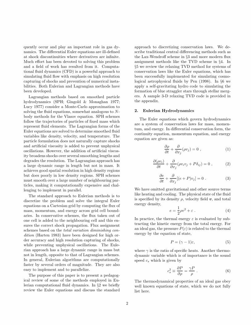
quently occur and play an important role in gas dy-namics. The differential Euler equations are ill-definedat shock discontinuities where derivatives are infinite.Much effort has been devoted to solving this problemand a field of work has resulted from it. Computa-tional fluid dynamics (CFD) is a powerful approach tosimulating fluid flow with emphasis on high resolutioncapturing of shocks and prevention of numerical insta-bilities. Both Eulerian and Lagrangian methods havebeen developed.

Lagrangian methods based on smoothed particlehydrodynamics (SPH; Gingold & Monaghan 1977;Lucy 1977) consider a Monte-Carlo approximation tosolving the fluid equations, somewhat analogous to N -body methods for the Vlasov equation. SPH schemesfollow the trajectories of particles of fixed mass whichrepresent fluid elements. The Lagrangian forms of theEuler equations are solved to determine smoothed fluidvariables like density, velocity, and temperature. Theparticle formulation does not naturally capture shocksand artificial viscosity is added to prevent unphysicaloscillations. However, the addition of artificial viscos-ity broadens shocks over several smoothing lengths anddegrades the resolution. The Lagrangian approach hasa large dynamic range in length but not in mass. Itachieves good spatial resolution in high density regionsbut does poorly in low density regions. SPH schemesmust smooth over a large number of neighbouring par-ticles, making it computationally expensive and chal-lenging to implement in parallel.

The standard approach to Eulerian methods is todiscretize the problem and solve the integral Eulerequations on a Cartesian grid by computing the flux ofmass, momentum, and energy across grid cell bound-aries. In conservative schemes, the flux taken out ofone cell is added to the neighbouring cell and this en-sures the correct shock propagation. Flux assignmentschemes based on the total variation diminishing con-

dition (Harten 1983) have been designed for high or-der accuracy and high resolution capturing of shocks,while preventing unphysical oscillations. The Eule-rian approach has a large dynamic range in mass butnot in length, opposite to that of Lagrangian schemes.In general, Eulerian algorithms are computationallyfaster by several orders of magnitude. They are alsoeasy to implement and to parallelize.

The purpose of this paper is to present a pedagog-ical review of some of the methods employed in Eu-lerian computational fluid dynamics. In §2 we brieflyreview the Euler equations and discuss the standard

approach to discretizing conservation laws. We de-scribe traditional central differencing methods such asthe Lax-Wendroff scheme in §3 and more modern fluxassignment methods like the TVD scheme in §4. In§5 we review the relaxing TVD method for systems ofconservation laws like the Euler equations, which hasbeen successfully implemented for simulating cosmo-logical astrophysical fluids by Pen (1998). In §6 weapply a self-gravitating hydro code to simulating theformation of blue straggler stars through stellar merg-ers. A sample 3-D relaxing TVD code is provided inthe appendix.

2. Eulerian Hydrodynamics

The Euler equations which govern hydrodynamicsare a system of conservation laws for mass, momen-tum, and energy. In differential conservation form, thecontinuity equation, momentum equation, and energyequation are given as:

∂ρ

∂t+

∂

∂xj(ρvj) = 0 , (1)

∂(ρvi)

∂t+

∂

∂xj(ρvivj + Pδij) = 0 , (2)

∂e

∂t+

∂

∂xj[(e+ P )vj ] = 0 . (3)

We have omitted gravitational and other source termslike heating and cooling. The physical state of the fluidis specified by its density ρ, velocity field v, and totalenergy density,

e =1

2ρv2 + ε . (4)

In practice, the thermal energy ε is evaluated by sub-tracting the kinetic energy from the total energy. Foran ideal gas, the pressure P (ε) is related to the thermalenergy by the equation of state,

P = (γ − 1)ε, (5)

where γ is the ratio of specific heats. Another thermo-dynamic variable which is of importance is the soundspeed cs which is given by

c2s ≡ ∂P

∂ρ=

γP

ρ. (6)

The thermodynamical properties of an ideal gas obeywell known equations of state, which we do not fullylist here.

2

The differential Euler equations require differen-tiable solutions and therefore, are ill-defined at jumpdiscontinuities where derivatives are infinite. In theliterature, nondifferentiable solutions are called weak

solutions. The differential form gives a complete de-scription of the flow in smooth regions, but the integralform is needed to properly describe shock discontinu-ities. In integral conservation form, the rate of changein mass, momentum, and energy is equal to the netflux of those conserved quantities through the surfaceenclosing a control volume. For simplicity of notation,we will continue to express conservation laws in differ-ential form, as a shorthand for the integral form.

2.1. Computational Fluid Dynamics

The standard approach to Eulerian computationalfluid dynamics is to discretize time into discrete stepsand space into finite volumes or cells, where the con-served quantities are stored. In the simplest case, theintegral Euler equations are solved on a Cartesian cu-bical lattice by computing the flux of mass, momen-tum, and energy across cell boundaries in discrete timesteps. Consider the Euler equations in vector differen-tial conservation form,

∂u

∂t+

∂F i(u)

∂xi= 0 , (7)

where u = (ρ, ρvx, ρvy, ρvz , e) contains the conservedphysical quantities and F (u) represents the flux terms.In practice, the conserved cell-averaged quantitiesun ≡ u(xn) and fluxes F n are defined at integergrid cell centres xn. The challenge is to use the cell-averaged values to determine the fluxes F n+1/2 at cellboundaries.

In the following sections, we describe flux assign-ment methods designed to solve conservation laws likethe Euler equations. For ease of illustration, we beginby considering a 1-D scalar conservation law,

∂u

∂t+

∂F (u)

∂x= 0 , (8)

where F (u) = vu and v is a constant advection veloc-ity. Equation (8) is referred to as a linear advectionequation and has the analytical solution,

u(x, t) = u(x− vt, 0) . (9)

The linear advection equation describes the transportof the quantity u at a constant velocity v.

In integral flux conservation form, the 1-D scalarconservation law can be written as

∂

∂t

∫ x2

x1

u(x, t)dx+

∫ x2

x1

∂F (u)

∂xdx = 0 , (10)

where x1 ≡ xn−1/2 and x2 ≡ xn+1/2 for our controlcells. Let F t

n+1/2 denote the flux of u through cellboundary xn+1/2 at time t. Note then that the secondintegral is simply equal to F t

n+1/2 − F tn−1/2. The rate

of change in the cell-integrated quantity∫

udx is equalto the net flux of u through the control cell. For adiscrete time step, the discretized solution for the cell-averaged quantity un is given by

ut+∆tn = ut

n −(

F tn+1/2 − F t

n−1/2

∆x

)

∆t . (11)

The physical quantity u is conserved since the fluxtaken out of one cell is added to the neighbouring cellwhich shares the same boundary. Note that Equa-tion (11) has the appearance of being a finite differ-ence scheme for solving the differential form of the 1-D scalar conservation law. This is why the differentialform can be used as a shorthand for the integral form.

3. Centered Finite-Difference Methods

Central-space finite-difference methods have ease ofimplementation but at the cost of lower accuracy andstability. For illustrative purposes, we start with asimple first-order centered scheme to solve the linearadvection equation. The discretized solution is givenby Equation (11) where the fluxes at cell boundaries,

F tn+1/2 =

F tn+1 + F t

n

2, (12)

are obtained by taking an average of cell-centeredfluxes F t

n = vutn. The discretized first-order centered

scheme can be equivalently written as

ut+∆tn = ut

n −(

F tn+1 − F t

n−1

2∆x

)

∆t . (13)

In this form, the discretization has the appearanceof using a central difference scheme to approximatespatial derivatives. Hence, centered schemes are of-ten referred to as central difference schemes. In prac-tice when using centered schemes, the discretization isdone on the differential conservation equation ratherthan the integral equation.

3

This simple scheme is numerically unstable and wecan show this using the von Neumann linear stabilityanalysis. Consider writing u(x, t) as a discrete Fourierseries:

utn =

1

N

N/2∑

k=−N/2

ctk exp

(

2πikn

N

)

, (14)

where N is the number of cells in our periodic box. Inplane-wave solution form, we can write this as

utn =

1

N

N/2∑

k=−N/2

c◦k exp

[

2πi(kn− ωt)

N

]

, (15)

where c◦k are the Fourier series coefficients for the ini-tial conditions u(x, 0). Equivalently, the time evolu-tion of the Fourier series coefficients in Equation (14)can be cast into a plane-wave solution of the form,

ctk = exp

(−2πiωt

N

)

c◦k , (16)

where the numerical dispersion relation ω(k) is com-plex in general. The imaginary part of ω represents thegrowth or decay of the Fourier modes while the realpart describes the oscillations. A numerical schemeis linearly stable if Im(ω) ≤ 0. Otherwise, the Fouriermodes will grow exponentially in time and the solutionwill blow up.

The exact solution to the linear advection equationcan be expressed in the form of Equation (9) or bya plane-wave solution where the dispersion relation isgiven by ω◦ = vk. The waves all travel at the samephase velocity ω◦/k = v in the exact case.

The centrally discretized linear advection equation(Equation 13) is exactly solvable. After m times steps,the time evolution of the independent Fourier modesis given by

cm∆tk = (1− iλ sinφ)

mc◦k , (17)

where λ ≡ v∆t/∆x and φ = 2πk∆x/N . The disper-sion relation is given by

ω =N

2π∆t

[

tan−1(λ sinφ) +i

2ln (1 + λ2 sin2 φ)

]

,

(18)For any time step ∆t > 0, the imaginary part of ω willbe > 0. The Fourier modes will grow exponentially intime and the solution will blow up. Hence, the first-order centered scheme is numerically unstable.

3.1. Lax-Wendroff Scheme

The Lax-Wendroff scheme (Lax &Wendroff 1960) issecond-order accurate in time and space and the ideabehind it is to stabilize the unstable first-order schemefrom the previous section. Consider a Taylor seriesexpansion for u(x, t+∆t):

u(x, t+∆t) = u(x, t)

+∂u

∂t∆t+

∂2u

∂t2∆t2

2+O(∆t3) , (19)

and replace the time derivatives with spatial deriva-tives using the conservation law to obtain

u(x, t+∆t) = u(x, t)

− ∂F

∂x∆t+

∂

∂x

(

∂F

∂u

∂F

∂u

∂u

∂x

)

∆t2

2+O(∆t3) . (20)

For the linear advection equation, the eigenvalue ofthe flux Jacobian is ∂F/∂u = v. Discretization usingcentral differences gives

ut+∆tn = ut

n − F tn+1 − F t

n−1

2∆x∆t

+

(

F tn+1 − F t

n

∆x− F t

n − F tn−1

∆x

)

v∆t2

2∆x. (21)

In conservation form, the solution is given by Equation(11), where the fluxes at cell boundaries are defined as

F tn+1/2 =

1

2

(

F tn+1 + F t

n

)

−(

F tn+1 − F t

n

) v∆t

2∆x. (22)

Compare this with the boundary fluxes for the first-order scheme (Equation 12). The Lax-Wendroffscheme obtains second-order fluxes,

F (2) = F (1) − ∂F

∂u

∂F

∂x

∆t

2, (23)

by modifying the first-order fluxes F (1) with a second-order correction.

The stability of the Lax-Wendroff scheme to solvethe linear advection equation can also be determinedusing the von Neumann analysis. The discretized Lax-Wendroff equation (Equation 21) is exactly solvableand after m time steps, the Fourier modes evolve ac-cording to

cm∆tk =

[

1− λ2(1− cosφ) − iλ sinφ]m

c◦k , (24)

4

Fig. 1.— The phase error Re(∆ω) and the amplica-tion factor Im(∆ω) for the Lax-Wendroff scheme withparameters N = 100, v = 1, and λ = 0.9.

where λ ≡ v∆t/∆x is called the Courant number andφ = 2πk∆x/N . The dispersion relation is given by

ω =N

2π∆ttan−1

[

λ sinφ

1− λ2(1 − cosφ)

]

+iN

4π∆tln

[

1− 4λ2(1 − λ2) sin4(

φ

2

)]

. (25)

It is important to note three things. First, the Lax-Wendroff scheme is conditionally stable provided thatIm(ω) ≤ 0, which is satisfied if

v∆t

∆x≤ 1 . (26)

This constraint is a particular example of a generalstability constraint known as the Courant-Friedrichs-

Lewyor (CFL) condition. The Courant number λ isalso referred to as the CFL number. Second, for λ = 1the dispersion relation is exactly identical to that ofthe exact solution and the numerical advection is ex-act. This is a special case, however, and it does not testthe ability of the Lax-Wendroff scheme to solve generalscalar conservation laws. Normally, one chooses λ < 1to satisfy the CFL condition. Lastly, for λ < 1 the dis-persion relation ω(k) for the Lax-Wendroff solution is

Fig. 2.— Lax-Wendroff scheme used to linearly advecta square wave (solid line) once (dashed line) and tentimes (dotted line) through a box of 100 grid cells atspeed v = 1.

different from the exact solution where ω◦ = vk. Thedispersion relation relative to the exact solution canbe parametrized by

∆ω ≡ ω − ω◦ . (27)

The second-order truncation of the Taylor series(Equation 20) results in a phase error Re(∆ω) which isa function of frequency. In the Lax-Wendroff solution,the waves are damped and travel at different speeds.Hence the scheme is both diffusive and dispersive.

In Figure (1) we plot the phase error Re(∆ω) andthe amplification term Im(∆ω) for the Lax-Wendroffscheme with parameters N = 100, v = 1, and λ = 0.9.A negative value of Re(∆ω) represents a lagging phaseerror while a positive value indicates a leading phaseerror. For the chosen CFL number, the high frequencymodes have the largest phase errors but they are highlydamped. Some of the modes having lagging phase er-rors are not highly damped. We will subsequently seehow this becomes important.

A rigourous test of the 1-D Lax-Wendroff schemeand other flux assignment schemes we will discuss isthe linear advection of a square wave. The challenge isto accurately advect this discontinuous function where

5

Fig. 3.— The phase error Re(∆ω) and the amplicationterm Im(∆ω) for the Lax-Wendroff scheme (boxes)and the first-order upwind scheme (crosses) with pa-rameters N = 100, v = 1, and λ = 0.9.

the edges mimic Riemann shock fronts. In Figure (2)we show how the Lax-Wendroff scheme does at advect-ing the square wave once (dashed line) and ten times(dotted line) through a periodic box of 100 grid cellsat speed v = 1 and λ = 0.9. Note that this schemeproduces numerical oscillations. Recall that a squarewave can be represented by a sum of Fourier or sinewaves. These waves will be damped and disperse whenadvected using the Lax-Wendroff scheme. Figure (1)shows that the modes having lagging phase errors arenot damped away. Hence, the Lax-Wendroff scheme ishighly dispersive and the oscillations in Figure (2) aredue to dispersion. We leave it as an exercise for thereader to advect a sine wave using the Lax-Wendroffscheme. Since there is only one frequency mode in thiscase, there will be no spurious oscillations due to dis-persion, but a phase error will be present. For a com-prehensive discussion on the family of Lax-Wendroffschemes and other centered schemes, see Hirsch (1990)and Laney (1998).

Fig. 4.— First-order upwind scheme used to linearlyadvect a square wave (solid line) once (dashed line)and ten times (dotted line) through a box of 100 gridcells at speed v = 1.

4. Upwind Methods

Upwind methods take into account the physical na-ture of the flow when assigning fluxes for the discretesolution. This class of flux assignment schemes, whoseorigin dates back to the work of Courant, Isaason, &Reeves (1952), has been shown to be excellent at cap-turing shocks and also being highly stable.

We start with a simple first-order upwind schemeto solve the linear advection equation. Consider thecase where the advection velocity is positive and flowis to the right. The flux of the physical quantity uthrough the cell boundary xn+1/2 will originate fromcell n. The upwind scheme proposes that, to first-order, the fluxes F t

n+1/2 at cell boundaries be taken

from the cell-centered fluxes F tn = vut

n, which is in theupwind direction. If the advection velocity is negativeand flow is to the left, the boundary fluxes F t

n+1/2

are taken from the cell-centered fluxes F tn+1 = vut

n+1.The first-order upwind flux assignment scheme can besummarized as follows:

F tn+1/2 =

F tn if v > 0 ,

F tn+1 if v < 0 .

(28)

6

Unlike central difference schemes, upwind schemes areexplicitly asymmetric.

The CFL condition for the first-order upwindscheme can be determined from the von Neumannanalysis. We consider the case of a positive advectionvelocity. After m time steps, the Fourier modes evolveaccording to

cm∆tk = [1− λ(1 − cosφ)− iλ sinφ]

mc◦k , (29)

where λ ≡ v∆t/∆x and φ = 2πk∆x/N . The disper-sion relation is given by

ω =N

2π∆ttan−1

[

λ sinφ

1− λ(1− cosφ)

]

+iN

4π∆tln

[

1− 4λ(1− λ) sin2(

φ

2

)]

. (30)

The CFL condition for solving the linear advectionequation with this scheme is to have λ ≤ 1, identical tothat for the Lax-Wendroff scheme. For λ < 1 the dis-persion relation ω(k) for the first-order upwind schemeis different from the exact solution where ω◦ = vk.This scheme is both diffusive and dispersive. Since itis only first-order accurate, the amount of diffusion islarge. In Figure (3) we compare the dispersion rela-tion of the upwind scheme to that of the Lax-Wendroffscheme. The Fourier modes in the upwind scheme alsohave phase errors but they will be damped away. Thelow frequency modes which contribute to the oscilla-tions in the Lax-Wendroff solution are more dampedin the upwind solution. Hence, one does not expect tosee oscillations resulting from phase errors.

In Figure (4) we show how the first-order upwindscheme does at advecting the Riemann shock wave.This scheme is well-behaved and produces no spuriousoscillations, but since it is only first-order, it is highlydiffusive. The first-order upwind scheme has the prop-erty of having monotonicity preservation. When ap-plied to the linear advection equation, it does not allowthe creation of new extrema in the form of spurious os-cillations. The Lax-Wendroff scheme does not have theproperty of having monotonicity preservation.

The flux assignment schemes that we have discussedso far are all linear schemes. Godunov (1959) showedthat all linear schemes are either diffusive or dispersiveor a combination of both. The Lax-Wendroff scheme ishighly dispersive while the first-order upwind schemeis highly diffusive. Godunov’s theorem also statesthat linear monotonicity preserving schemes are only

Fig. 5.— The TVD scheme using the minmod fluxlimiter is applied to the advection of a square wave.

first-order accurate. In order to obtain higher orderaccuracy and prevent spurious oscillations, nonlinearschemes are needed to solve conservation laws.

4.1. Total Variation Diminishing Schemes

Harten (1983) proposed the total variation di-

minishing (TVD) condition which guarantees thata scheme have monotonicity preservation. ApplyingGodunov’s theorem, we know that all linear TVDschemes are only first-order accurate. In fact, the onlylinear TVD schemes are the class of first-order up-wind schemes. Therefore, higher order accurate TVDschemes must be nonlinear.

The TVD condition is a nonlinear stability condi-tion. The total variation of a discrete solution, definedas

TV (ut) =

N∑

i=1

|uti+1 − ut

i| , (31)

is a measure of the overall amount oscillations in u.The direct connection between the total variation andthe overall amount of oscillations can be seen in theequivalent definition

TV (ut) = 2(

∑

umax −∑

umin

)

, (32)

7

Fig. 6.— The TVD scheme using the superbee fluxlimiter is applied to the advection of a square wave.

where each maxima is counted positively twice andeach minima counted negatively twice (See Laney1998). The formation of spurious oscillations will con-tribute new maxima and minima and the total varia-tion will increase. A flux assignment scheme is said tobe TVD if

TV (ut+∆t) ≤ TV (ut) , (33)

which signifies that the overall amount of oscillations isbounded. In linear flux-assignment schemes, the vonNeumann linear stability condition requires that theFourier modes remain bounded. In nonlinear schemes,the TVD stability condition requires that the totalvariation diminishes.

We now describe a nonlinear second-order accurateTVD scheme which builds upon the first-order mono-tone upwind scheme described in the previous section.The second-order accurate fluxes F t

n+1/2 at cell bound-

aries are obtained by taking first-order fluxes F(1),tn+1/2

from the upwind scheme and modifying it with a sec-ond order correction. First consider the case where theadvection velocity is positive. The first-order upwind

flux F(1),tn+1/2 comes from the averaged flux F t

n in cell n.

Fig. 7.— The TVD scheme using the Van Leer fluxlimiter is applied to the advection of a square wave.

We can define two second-order flux corrections,

∆FL,tn+1/2 =

F tn − F t

n−1

2, (34)

∆FR,tn+1/2 =

F tn+1 − F t

n

2, (35)

using three local cell-centered fluxes. We use cell nand the cells immediately left and right of it. If theadvection velocity is negative, the first-order upwindflux comes from the averaged flux F t

n+1 in cell n + 1.In this case, the second-order flux corrections,

∆FL,tn+1/2 = −F t

n+1 − F tn

2, (36)

∆FR,tn+1/2 = −F t

n+2 − F tn+1

2. (37)

are based on cell n+1 and the cells directly adjacent toit. Near extrema where the corrections have oppositesigns, we impose no second-order correction and theflux assignment scheme reduces to first-order. A fluxlimiter φ is then used to determine the appropriatesecond-order correction,

∆F tn+1/2 = φ(∆FL,t

n+1/2,∆FR,tn+1/2) , (38)

8

which still maintains the TVD condition. The second-order correction is added to the first-order fluxes to getsecond-order fluxes. The first-order upwind schemeand second-order TVD scheme will be referred toas monotone upwind schemes for conservation laws

(MUSCL).

Time integration is performed using a second-orderRunge-Kutta scheme. We first do a half time step,

ut+∆t/2n = ut

n −(

F tn+1/2 − F t

n−1/2

∆x

)

∆t

2, (39)

using the first-order upwind scheme to obtain the half-step values ut+∆t/2. A full time step is then computed,

ut+∆tn = ut

n −

Ft+∆t/2n+1/2 − F

t+∆t/2n−1/2

∆x

∆t , (40)

using the TVD scheme on the half-step fluxes F t+∆t/2.The reader is encouraged to show that is second-orderaccurate.

We briefly discuss three TVD limiters. The min-mod flux limiter chooses the smallest absolute valuebetween the left and right corrections:

minmod(a, b) = 12 [sign(a) + sign(b)]min(|a|, |b|) .

(41)The superbee limiter (Roe 1985) chooses between thelarger correction and two times the smaller correction,whichever is smaller in magnitude:

superbee(a, b) =

minmod(a, 2b) if |a| ≥ |b| ,

minmod(2a, b) otherwise .(42)

The Van Leer limiter (Van Leer 1974) takes the har-monic mean of the left and right corrections:

vanleer(a, b) =2ab

a+ b. (43)

The minmod limiter is the most moderate of allsecond-order TVD limiters. In Figure (5) we see thatit does not do much better than first-order upwindfor the square wave advection test. Superbee choosesthe maximum correction allowed under the TVD con-straint. It is especially suited for piece-wise linearconditions and is the least diffusive for this particulartest, as can be seen in Figure (6). Note that no ad-ditional diffusion can be seen by advecting the squarewave more than once through the box. It can be shown

that the minmod and superbee limiters are extremecases which bound all other second-order TVD lim-iters. The Van Leer limiter differs from the previoustwo in that it is analytic. This symmetrical approachfalls somewhere inbetween the other two limiters interms of moderation and diffusion, as can be seen inFigure (7). It can be shown that the CFL conditionfor the second-order TVD scheme is to have λ < 1.For a comprehensive discussion on TVD limiters, seeHirsch (1990) and Laney (1998).

5. Relaxing TVD

We now describe a simple and robust method tosolve the Euler equations using the monotone upwindscheme for conservation laws (MUSCL) from the pre-vious section. The relaxing TVD method (Jin & Xin1995) provides high resolution capturing of shocks us-ing computationally inexpensive algorithms which arestraightforward to implement and to parallelize. Ithas been successfully implemented for simulating cos-mological astrophysical fluids by Pen (1998).

The MUSCL scheme is straightforward to apply toconservation laws like the advection equation since thevelocity alone can be used as a marker of the direc-tion of flow. However, applying the MUSCL scheme tosolve the Euler equations is made difficult by the factthat the momentum and energy fluxes depend on thepressure. In order to determine the direction upwind ofthe flow, it becomes necessary to calculate the flux Ja-cobian eigenvectors using Riemann solvers. This steprequires computationally expensive algorithms. Therelaxing TVD method offers an attractive alternative.

5.1. 1-D Scalar Conservation Law

We first present a motivation for the relaxingscheme by again considering the 1-D scalar conser-vation law. The MUSCL scheme for solving the linearadvection equation is explicitly asymmetric in that itdepends on the sign of the advection velocity. We nowdescribe a symmetrical approach which applies to ageneral advection velocity.

The flow can be considered as a sum of a right-moving wave uR and a left-moving wave uL. For apositive advection velocity, the amplitude of the left-moving wave is zero and for a negative advection ve-locity, the amplitude of the right-moving wave is zero.

9

In compact notation, the waves can be defined as:

uR =

(

1 + v/c

2

)

u , (44)

uL =

(

1− v/c

2

)

u , (45)

where c = |v|. The two waves are traveling in oppositedirections with advection speed c and can be describedby the advection equations:

∂uR

∂t+

∂

∂x(cuR) = 0 , (46)

∂uL

∂t− ∂

∂x(cuL) = 0 . (47)

The MUSCL scheme is straightforward to apply tosolve Equations (46) and (47) since the upwind direc-tion is left for the right-moving wave and right for theleft-moving wave. The 1-D relaxing advection equa-tion then becomes

∂u

∂t+

∂FR

∂x− ∂FL

∂x= 0 . (48)

where FR = cuR and FL = cuL. For the discretizedsolution given by Equation (11), the boundary fluxes

F tn+1/2 are now a sum of the fluxes FR,t

n+1/2 and FL,tn+1/2

from the right-moving and left-moving waves, respec-tively. Note that the relaxing advection equation willcorrectly reduce to the linear advection equation forany general advection velocity.

Using this symmetrical approach, a general algo-rithm can be written to solve the linear advectionequation for an arbitrary advection velocity. Thisscheme is indeed inefficient for solving the linear ad-vection equation since one wave will have zero am-plitude. However, the Euler equations can have bothright-moving and left-moving waves with non-zero am-plitudes.

5.2. 1-D Systems of Conservation Laws

We now discuss the 1-D relaxing TVD scheme andlater generalize it to higher spatial dimensions. Con-sider a 1-D system of conservation laws,

∂u

∂t+

∂F (u)

∂x= 0 , (49)

where for the Euler equations, we have u = (ρ, ρv, e)and F (u) the corresponding flux terms. We now re-place the vector conservation law with the relaxation

system∂u

∂t+

∂

∂x(cw) = 0 , (50)

∂w

∂t+

∂

∂x(cu) = 0 , (51)

where c(x, t) is a free positive function called the freez-ing speed. The relaxation system contains two coupledvector linear advection equations. In practice, we setw = F (u)/c and use it as an auxiliary vector to cal-culate fluxes. Equation (50) reduces to our 1-D vectorconservation law and Equation (51) is a vector conser-vation law for w.

In order to solve the relaxed system, we decouplethe equations through a change of variables:

uR =u+w

2, (52)

uL =u−w

2, (53)

which then gives us

∂uR

∂t+

∂

∂x(cuR) = 0 , (54)

∂uL

∂t− ∂

∂x(cuL) = 0 . (55)

Equations (54) and (55) are vector linear advectionequations, which can be interpreted as right-movingand left-moving flows with advection speed c. Notethe similarity with their scalar counterparts, Equa-tions (46) and (47). The 1-D vector relaxing conser-vation law for u becomes

∂u

∂t+

∂FR

∂x− ∂FL

∂x= 0 , (56)

where FR = cuR and FL = cuL. The vector relaxingequation can now be solved by applying the MUSCLscheme to Equations (54) and (55). Again, note thesimilarity between the vector relaxing equation and itsscalar counterpart, Equation (48).

The relaxed scheme is TVD under the constraintthat the freezing speed c be greater than the charac-teristic speed given by the largest eigenvalue of the fluxJacobian ∂F (u)/∂u. For the Euler equations, this issatisfied for

c = |v|+ cs . (57)

Jin & Xin (1995) considered the freezing speed to bea positive constant in their relaxing scheme while we

10

generalize it to be a positive function. Time integra-tion is again performed using a second-order Runge-Kutta scheme and the time step is determined by sat-isfying the CFL condition,

cmax∆t

∆x≤ 1 . (58)

Note that a new freezing speed is computed for eachpartial step in the Runge-Kutta scheme. The CFLnumber λ = cmax∆t/∆x should be chosen such that

cmax will be larger than max(ctn) and max(ct+∆t/2n ).

We now summarize the steps needed to numericallysolve the 1-d Euler equations. At the beginning ofeach partial step in the Runge-Kutta time integra-tion scheme, we need to calculate the cell-averagedvariables defined at grid cell centres. First for thehalf time step, we calculate the fluxes F (ut

n) and thefreezing speed ctn. We then set the auxiliary vectorwt

n = F (utn)/c

tn and construct the right-moving waves

uR,tn and left-moving waves uL,t

n . The half time stepis given by

ut+∆t/2n = ut

n −(

F tn+1/2 − F t

n−1/2

∆x

)

∆t

2, (59)

whereF t

n+1/2 = FR,tn+1/2 − F

L,tn+1/2 . (60)

The first-order upwind scheme is used to computefluxes at cell boundaries for the right-moving and left-moving waves. For the full time step, we construct the

right-moving waves uR,t+∆t/2n and left-moving waves

uL,t+∆t/2n , using the half-step values of the appropri-

ate variables. The full time step,

ut+∆tn = ut

n −

Ft+∆t/2n+1/2 − F

t+∆t/2n−1/2

∆x

∆t , (61)

is computed using the second-order TVD scheme. Thiscompletes the updating of ut to ut+∆t.

We have found that a minor modification to theimplementation described above gives more accurateresults. Consider writing the flux of the right-movingand left-moving waves as:

FR = cGR , (62)

F L = cGL , (63)

where GR is the flux of µR = uR/c and GL is theflux of µL = uL/c. The linear advection equations for

µR and µL are similar to Equations (54) and (55), butwhere we replace uR with µR and uL with µL. Foreach partial step in the Runge-Kutta scheme, the netfluxes at cell boundaries are then taken to be

F n+1/2 = cn+1/2(GRn+1/2 −GL

n+1/2) , (64)

where we use cn+1/2 = (cn+1+ cn)/2. In practice, thismodified implementation has been found to resolveshocks with better accuracy in certain cases. Notethat the two different implementations of the relaxingTVD scheme are identical when a constant freezingspeed is used.

5.3. Multi-Dimensional Systems of Conserva-

tion Laws

The 1-D relaxing TVD scheme can be generalizedto higher dimensions using the dimensional splittingtechnique by Strang (1968). In three dimensions, theEuler equations can be dimensionally split into threeseparate 1-D equations which are solved sequentially.Let the operator Li represent the updating of ut tout+∆t by including the flux in the i direction. We firstcomplete a forward sweep,

ut+∆t = LzLyLxut , (65)

and then perform a reverse sweep

ut+2∆t = LxLyLzut+∆t , (66)

using the same time step ∆t to obtain second-orderaccuracy. We will refer to the combination of the for-ward and reverse sweeps as a double sweep.

A more symmetrical sweeping pattern can be usedby permutating the sweeping order when completingthe next double time step. The dimensional splittingor operator splitting technique can be summarized asfollows:

ut2 = ut1+2∆t1 = LxLyLzLzLyLxut1 , (67)

ut3 = ut2+2∆t2 = LzLxLyLyLxLzut2 , (68)

ut4 = ut3+2∆t3 = LyLzLxLxLzLyut3 , (69)

where ∆t1, ∆t2, and ∆t3 are newly determined timesteps after completing each double sweep.

The CFL condition for the 3-D relaxing TVDscheme is similarly given by Equation (58), but with

cmax = max[(cx)max, (cy)max, (cz)max] . (70)

11

r

0

0.2

0.4

0.6

0.8

1

0

0.2

0.4

0.6

0.8

1

0 50 100

0

0.2

0.4

0.6

0.8

1

Fig. 8.— Sedov-Taylor blast wave test conducted in abox with 2563 cells. The data points are taken froma random subset of cells and the solid lines are theanalytical self-similar solutions.

where ci = |vi| + cs. Note that since max(|vi|) is onaverage a factor of

√3 smaller than max(|v|), a di-

mensionally split scheme can use a longer time stepcompared to an un-split scheme.

The dimensional splitting technique also has otheradvantages. The decomposition into a 1-D problem al-lows one to write short 1-D algorithms, which are easyto optimize to be cache efficient. A 3-D hydro code isstraightforward to implement in parallel. When sweep-ing in the x direction, for example, one can break upthe data into 1-D columns and operate on the indepen-dent columns in parallel. A sample 3-D relaxing TVDcode, implemented in parallel using OpenMP direc-tives, is provided in the appendix.

6. Sedov-Taylor Blast Wave Test for 3-D Hy-

dro

A rigourous and challenging test for any 3-D Eule-rian or Lagrangian hydrodynamic code is the Sedov-Taylor blast wave test. We set up the simulation boxwith a homogeneous medium of density ρ1 and neg-ligible pressure and introduce a point-like supply ofthermal energy E◦ in the centre of the box at time

r

0

0.2

0.4

0.6

0.8

1

0

0.2

0.4

0.6

0.8

1

100 105 110 115

0

0.2

0.4

0.6

0.8

1

Fig. 9.— A closeup of the Sedov-Taylor blast wave.The resolution of the shock front is roughly two gridcells and the anisotropic scatter is less than one gridcell.

t = 0. The challenge is to accurately capture thestrong spherical shock wave which sweeps along ma-terial as it propagates out into the ambient medium.The Sedov-Taylor test is used to model nuclear-typeexplosions. In astrophysics, it is often used as a basicsetup to model supernova explosions and the evolutionof supernova remnants (See Shu 1992).

The analytical Sedov solution uses the self-similarnature of the blast wave expansion (See Landau & Lif-shitz 1987). Consider a frame fixed relative to the cen-tre of the explosion. The spherical shock front propa-gates outward and the distance from the origin is givenby

rsh(t) = ξ◦

(

E◦t2

ρ1

)1/5

, (71)

where ξ◦ = 1.15 for an ideal gas with γ = 5/3. Thevelocity of the shock vsh = ∂rsh/∂t is given by

vsh(t) =2

5

rsh(t)

t. (72)

Since the ambient medium has negligible pressure, theshocks will be very strong. The density ρ2, velocity v2,

12

and pressure P2 directly behind the shock front are:

ρ2 =

(

γ + 1

γ − 1

)

ρ1 , (73)

v2 =

(

2

γ + 1

)

vsh , (74)

P2 =

(

2

γ + 1

)

ρ1v2sh . (75)

The immediate post-shock gas density is constant intime, while the shocked gas velocity v2 and pressure P2

decrease as t−3/5 and t−6/5, respectively. The full ana-lytical Sedov-Taylor solutions can be found in Landau& Lifshitz (1987).

The 3-D relaxing TVD code based on the van Leerflux limiter is applied to capturing the Sedov-Taylorblast wave. We set up a box with 2563 cells and con-stant initial density ρ1 = 1. At time t = 0, we inject asupply of thermal energy E◦ = 105 into one cell at thecentre of the box. The simulation is stopped at timet = 283, in which the shock front has propagated out toa distance of rsh = 110 cells from the centre. In Figure(8) and (9) we plot the radial distributions of density,momentum, and pressure, normalized to ρ2, ρ2v2, andP2 respectively. The data points are taken from a ran-dom subset of cells and the solid lines are the analyticalSedov-Taylor solutions. Despite solving a sphericallysymmetric problem on an explicitly non-rotationallyinvariant Cartesian grid, the anisotropic scatter in theresults is small. The distance of the shock front fromthe centre of the explosion as a function of time is in-deed given by Equation (71), demonstrating that the3-D relaxing TVD code ensures the correct shock prop-agation. The resolution of the shock front is roughlytwo grid cells. The numerical shock jump values of ρ2,v2, and P2 are resolution dependent and come close tothe theoretical values for our test with 2563 cells. Weleave it as an exercise for the reader to test the codeusing the minmod and superbee flux limiters.

7. Self-Gravitating Hydro for Astrophysical

Applications

For astrophysical applications, both hydrodynami-cal and gravitational forces are included. The gravi-tational forces arise from the self-gravity of the fluidand can also come from an external field. The Eulerequations with the gravitational source terms included

are given as:

∂ρ

∂t+

∂

∂xj(ρvj) = 0 , (76)

∂(ρvi)

∂t+

∂

∂xj(ρvivj + Pδij) = −ρ

∂φ

∂xi, (77)

∂e

∂t+

∂

∂xj[(e + P )vj ] = −ρvi

∂φ

∂xi. (78)

where φ is the gravitational potential. Poisson’s equa-tion,

∇2φ = 4πGρ , (79)

relates the gravitational potential to the density field.The general solution can be written as

φ(x) =

∫

ρ(x′)w(x − x′)d3x′ , (80)

where the kernel is given by

w(x) = − G

|x| . (81)

In the discrete case, the integral in Equation (80) be-comes a sum and Poisson’s equation can be solved us-ing fast Fourier transforms (FFT) to do the convolu-tion. The forces are then calculated by finite differenc-ing the potential (See Hockney & Eastwood 1988).

The addition of gravatitational source terms in theEuler equations is easily handled using the operatorsplitting technique described in §5.3. Consider thedouble sweep:

ut+2∆t = LxLyLzGGLzLyLxut , (82)

where the operator Li represents the updating of u byincluding the flux in the i direction and the operatorG represents the gravitational acceleration of the fluid.During the gravitational step, the flux terms in theEuler equations are ignored. The density distributiondoes not change and only the fluid momenta and totalenergy density are updated.

7.1. Astrophysical Formation of Blue Strag-

glers Through Stellar Collisions

The stellar density in the cores of globular and openclusters is high enough for stellar collisions to takeplace with significant frequency (Hills & Day 1976).Current observations and simulations suggest that themerger of two main sequence stars produces a blue

13

straggler (Sills et al. 1997; Sandquist, Bolte, & Hern-quist 1997). The blue stragglers are out-lying mainsequence stars which lie beyond the main sequenceturnoff in the colour-magnitude diagram (CMD) of astar cluster. The blue stragglers are more massive,brighter, and bluer than the turnoff stars. Since moremassive stars evolve faster than lower mass stars andare not expected to lie beyond the turnoff, this sug-gests that blue stragglers must have formed more re-cently.

In principle the merger of two main sequence starscan produce a young remnant star provided that sig-nificant mixing occurs in the process. The mixing pro-duces a higher hydrogen fraction in the core of theremnant than that of the parent stars which have al-ready burnt most of the hydrogen to helium in theircores. Benz & Hills (1987) used low resolution SPHsimulations with ∼ 103 particles to simulate the merg-ing of n = 3/2 polytropes and found that they fullymixed. However, medium resolution SPH simulationswith ∼ 104 particles of n = 3/2 or n = 3 polytropesshowed only weak mixing (Lombardi, Rasio, & Shapiro1996; Sandquist, Bolte, & Hernquist 1997). It is worthnoting that n = 3/2 polytropes are more representa-tive of low mass main sequence stars with large convec-tive envelopes while n = 3 polytropes resemble mainsequence stars near the turnoff which have little massin their convective envelopes. High resolution SPHsimulations involving ∼ 105 − 106 particles have nowbeen applied to simulating stellar collisions (Sills et a.2002).

The merging stars process is mostly subsonic andstrong shocks are not expected. In the absence ofshocks, SPH particles will follow flow lines of constantentropy due to the Lagrangian nature of the method.As a result, the particles may experience sedimenta-tion. In addition, the mixing can also depend on theadopted smoothing length and the form of artificialviscosity. For a SPH fluid, the Reynolds number isof order (Np/Ns)

1/3, where Np is the total number ofparticles and Ns is the number of particles over whichthe smoothing is done. For Np ∼ 105 and Ns ∼ 102,the Reynolds number is ∼ 10. However, a fluid with alow Reynolds number will tend to experience laminarflow. Hence, SPH may under mix.

It is a worthwhile exercise to model the mergingprocess using Eulerian hydrodynamical simulations.The differences between Eulerian and Lagrangian ap-proaches may lead to very different results on mixing.As of present, no such work has been reported in the

Fig. 10.— The advection of a self-gravitating poly-trope in a periodic box with 2563 cells. We comparethe mass and entropy profiles of the initial (solid line)and advected polytrope after 1000 timesteps in whichthe polytrope has moved 256 cells in each direction.

literature.

7.2. Numerical Method

We consider the off-axis collision of two main se-quence stars with M = 0.8M⊙ and R = 0.955R⊙,which are modeled using n = 3 polytropes. A poly-trope with polytropic index n has equilibrium densityand pressure profiles which are related by

P ∝ ρ1+1/n . (83)

The density profile is determined by solving the Lane-Emden equation (See Chandrasekhar 1957). We adoptan ideal gas equation of state with adiabatic indexγ = 5/3. Note that for an n = 3 polytrope, 90%of the total mass is contained within r . 0.5R. Wedefine the dynamical time to be,

τdyn ≡ 1√Gρ̄

, (84)

where ρ̄ is the average density. For the chosen parentstars, the dynamical time is approximately one physi-cal hour.

14

0 100 200 300 400 5000

100

200

300

400

500

x

0 100 200 300 400 5000

100

200

300

400

500

x

0 100 200 300 400 5000

100

200

300

400

500

x

0 100 200 300 400 5000

100

200

300

400

500

x

Fig. 11.— Snapshots of the merging process taken attime t = 0, 2, 4, and 8 τdyn. The density contours arespaced logarithmically with 2 per decade and covering3 decades down from the maximum.

The collision is simulated in a box with 512× 512×256 cells and the orbital plane coincides with the x−yplane. Initially, each parent star has a radius of 96 gridcells. The stars are set up on zero-energy parabolicorbits with a pericentre separation equal to 0.25R.The initial trajectories are calculated assuming pointmasses. In an Eulerian simulation, the vacuum cannothave zero density. We set the minimum density of thecells to be 10−8 of the central density of the parentstars. The hydrodynamics is done in a non-periodicbox with vacuum boundary conditions.

7.3. Numerical Results

A non-trivial test of a self-gravitating Eulerian hy-dro code is the advection of an object in hydrostaticequilibrium. The challenge is to maintain the equilib-rium profile over a large number of time steps. One ofthe parent stars is placed in a periodic box with 2563

cells and given some initial momentum. We make thetest rigorous by having the polytrope move in all threedirections. In Figure 10 we compare the mass and en-tropy profiles of the initial and advected polytrope.The entropic variable A ≡ P/ργ is used in place ofthe specific entropy. The parameter A◦ is defined to

Fig. 12.— Thermodynamic profiles of the merger rem-nant (solid) and the parent stars (dashed). Units arecgs. The radial plot is included for comparison.

be the minimum entropy of the parent polytrope. Af-ter 1000 timesteps in which the polytrope has moved256 cells in each direction, the advected polytrope hasstill retained its equilibrium profile. Shock heating canoccur in the outer envelope as the polytrope movesthrough the false vacuum. However, by setting thedensity of the false vacuum to be 10−8 of the centraldensity of the polytrope, we can minimize the spuriousshock heating.

In Figure 11 we show four snapshots of the mergingprocess taken at time t = 0, 2, 4, and 8 τdyn. The 2-Ddensity maps are created by averaging over 4 planestaken about the orbital mid-plane. The density con-tours are spaced logarithmically with 2 per decade andcovering 3 decades down from the maximum. The par-ent stars are initially separated by 3.75R and placedon zero-energy orbits with a pericentre separation of0.25R. During the collision process, the outer en-velopes of the parent stars are shock heated and mate-rial gets ejected. In less than 10 τdyn, the merger rem-nant establishes hydrostatic equilibrium. The mergerremnant is a rotating oblate with mass approximately90% of the combined mass of the parent stars. A largefraction of the mass loss is due to the vacuum bound-ary conditions. Ejected material do not have the op-

15

portunity to fall back onto the merger remnant. How-ever, the additional mass loss in the envelope does notpresent a problem since we are interested in the ques-tion of mixing in the interior of the star.

In Figure 12 we plot the thermodynamic profiles ofthe merger remnant and the parent stars. The centraldensity and pressure in the core of the merger remnantis lower than the corresponding values in the parentstars by approximately half. The entropy floor hasrisen by a factor of 1.6. Shock heating is expected tobe minimal in the core so a change in entropy suggeststhat some mixing has taken place. However, it is diffi-cult to quantify the amount of mixing from examiningthe thermodynamic profiles alone.

7.4. Future Work

To help address the question of mixing, we are im-plementing a particle-mesh (PM) scheme where testparticles can be used to track passively advected quan-tities such as chemical composition. Initially, each par-ent star is assigned a large number of particles withknown chemical composition. The test particles arepassively advected along velocity field lines. For eachtime step, the velocity of each particle is interpolatedfrom the grid using a ”cloud-in-cell” (CIC) scheme(Hockney & Eastwood 1988) and the equations of mo-tions are solved using second-order Runge-Kutta in-tegration. The CIC interpolation scheme is also usedto determine the local density, pressure, and entropyassociated with each particle. With this setup, wehave the benefit of being able to track thermodynamicquantities like in an SPH scheme but avoid the undermixing problem since the fluid equations are solvedusing the Eulerian scheme.

Future work (Trac, Sills, & Pen 2003) will havehigher resolution simulations. Collisions will be simu-lated in a box with 1024×1024×512 cells. Each parentstar will have a radius of 192 grid cells and be assigned2563 test particles. We will also be doing a detailedcomparison between Eulerian and SPH simulations ofstellar mergers.

The self-gravitating hydro code used for the simu-lations is very memory friendly. For the 10242 × 512grid, 10 GB is required to store the hydro variables, 2GB for the potential, and less than 1 GB for the testparticles. For every double timestep, approximately1000 floating point operations per grid cell is needed tocarry out the TVD hydro calculations. The potentialis computed once for every double step and this re-

quires two FFTs. Since Eulerian codes are very mem-ory friendly, have low floating point counts, are eas-ily parallelized, and scale very well on shared-memory,multiple-processor machines, they can be used to runvery high resolution simulations.

8. Summary

We have presented several numerical schemes forsolving the linear advection equation and given theCFL stability conditions for each scheme. We haveimplemented the relaxing TVD scheme to solve theEuler system of conservation laws. The second-orderaccurate TVD scheme provides high resolution captur-ing of shocks, as can be seen in the Riemann shock testand the Sedov-Taylor blast wave test. The 1-D relax-ing TVD scheme can be easily generalized to higherdimensions using the dimensional splitting technique.A dimensionally split scheme can use longer time stepsand is straightforward to implement in parallel. Wehave presented a sample astrophysical application. A3-D self-gravitating Eulerian hydro code is used to sim-ulate the formation of blue straggler stars through stel-lar mergers. We hope to have convinced the readerthat Eulerian computational fluid dynamics is a pow-erful approach to simulating complex fluid flows be-cause it is simple, fast, and accurate.

We thank Joachim Stadel and Norm Murray forcomments and suggestions on the writing and editingof this paper. We also thank Alison Sills, Phil Arras,and Chris Matzner for discussions on stellar mergers.

REFERENCES

Benz, W. & Hills, J. G., 1987, ApJ, 323, 614

Chandrasekhar, S., 1957, An Introduction to theStudy of Stellar Structure (New York: Dover Pub-lications)

Courant, R., Isaacson, E., & Reeves, M., 1952, Comm.Pure and Applied Math., 5, 243

Gingold, R. A. & Monaghan, J. J., 1977, MNRAS,181, 375

Godunov, S. K., 1959, Math. Sbornik, 47, 271

Harten, A., 1983, J. Comp. Phys., 49, 357

Hill, J. G. & Day, C. A., 1976, ApJ, 17, 87

16

Hirsch, C., 1990, Numerical Computation of Internaland External Flows, vol. 2: Computational Meth-ods for Inviscid and Viscous Flows (New York: JohnWiley)

Hockney, R. W. & Eastwood, J. W., 1988, ComputerSimulation Using Particles (Philadelphia: IOPPublishing)

Jin, S. & Xin, Z., 1995, Comm. Pure and AppliedMath., 48, 235

Landau, L. D. & Lifshitz, E. M., 1987, Fluid Mechanics(2nd ed.; Oxford: Pergamon Press)

Laney, C. B., 1998, Computational Gas Dyanamics(Cambridge: Cambridge University Press)

Lax, P. D. & Wendroff, B., 1960, Comm. Pure andApplied Math., 10, 537

Lombardi, J. C., Jr., Rasio, F. A., & Shapiro, S. L,1996, ApJ, 468, 797

Lucy, L. B., 1977, AJ, 82, 1013

Pen, U., 1998, ApJS, 115, 19

Roe, P. L.,1985, in Large-Scale Computations in FluidMechanics, Lectures in Applied Mathematics, eds.B. E. Engquist, S. Osher, & R. C. J. Somerville(Providence, RI: American Mathematical Society)

Sandquist, E. L., Bolte, M., & Hernquist, L., 1997,ApJ, 477, 335

Shu, F. H., 1992, Gas Dynamics (Mill Valley: Univer-sity Science Books)

Sills, A., Adams, T., Davies, M. B., & Bate, M. R.,2002, MNRAS, 332, 49

Sills, A., Lombardi, J. C., Jr., Bailyn, C. D., Demar-que, P. D., Rasio, F. A., & Shapiro, S. L., 1997,ApJ, 487, 290

Strang, G., 1968, SIAM J. Num. Anal., 5, 506

Van Leer, B., 1974, J. Comp. Phys., 14, 361

This 2-column preprint was prepared with the AAS LATEX

macros v5.0.

17

A. 3-D Relaxing TVD code

We provide a sample 3-D relaxing TVD code written in Fortran 90. The code is implemented using OpenMPdirectives to run in parallel on shared memory machines. The code is fast and memory friendly. The array u(a,i,j,k)stores the five conserved hydro quantities a = (ρ, ρvx, ρvy, ρvz, e) for each cell (i,j,k) in the Cartesian cubical latticewith side length nc. For each sweep, we first call the subroutine timestep to determine the appropriate time step dtwhich satisfies the CFL condition. The updating of u by including the flux in the x direction is performed by thesweepx subroutine. The data array u is divided into 1-D array sections u1d(a,i) which are operated on by the relaxingsubroutine. The independent columns are distributed amongst multiple processors on a shared memory machine bythe OpenMP directives.

The relaxing TVD subroutine in this sample code is written for ease of readability and therefore, is not fullyoptimized. At the beginning of each partial step in the Runge-Kutta time integration scheme, the cell-averagedvariables defined at grid cell centres are calculated by the averageflux subroutine. The fluxes at cell boundaries forthe right-moving and left-moving waves are stored in fr and fl, respectively. We have implemented the minmod,superbee, and Van Leer flux limiters and the user of the code can easily switch between them.

We have provided some initial conditions for the Sedov-Taylor blast wave test. The reader is encouraged to test thecode and compare how the various flux limiters do at resolving strong shocks. This sample code does not implementthe modified relaxing TVD scheme described at the end of §5.2, which has been found work very well with the VanLeer flux limiter but unstable with superbee for the 3-D Sedov Taylor test. We have found that the superbee limiteris often unstable for 3-D fluid simulations. Please contact the authors regarding any questions on the implementationof the relaxing TVD algorithm.

program mainimplicit noneinteger, parameter :: nc=64,hc=nc/2real, parameter :: gamma=5./3,cfl=0.9

real, dimension(5,nc,nc,nc) :: u

integer nsw,stopsimreal t,tf,dt,E0,rmax

t=0dt=0nsw=0stopsim=0

E0=1e5rmax=3*hc/4tf=sqrt((rmax/1.15)**5/E0)

call sedovtaylordocall timestepcall sweepxcall sweepycall sweepzcall sweepzcall sweepycall sweepx

18

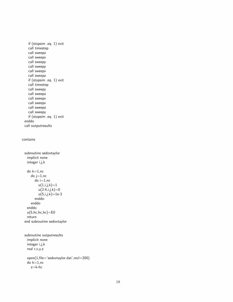
if (stopsim .eq. 1) exitcall timestepcall sweepzcall sweepxcall sweepycall sweepycall sweepxcall sweepzif (stopsim .eq. 1) exitcall timestepcall sweepycall sweepzcall sweepxcall sweepxcall sweepzcall sweepyif (stopsim .eq. 1) exit

enddocall outputresults

contains

subroutine sedovtaylorimplicit noneinteger i,j,k

do k=1,ncdo j=1,ncdo i=1,ncu(1,i,j,k)=1u(2:4,i,j,k)=0u(5,i,j,k)=1e-3

enddoenddo

enddou(5,hc,hc,hc)=E0return

end subroutine sedovtaylor

subroutine outputresultsimplicit noneinteger i,j,kreal r,x,y,z

open(1,file=’sedovtaylor.dat’,recl=200)do k=1,ncz=k-hc

19

do j=1,ncy=j-hcdo i=1,ncx=i-hcr=sqrt(x**2+y**2+z**2)write(1,*) r,u(:,i,j,k)

enddoenddo

enddoclose(1)return

end subroutine outputresults

subroutine timestepimplicit noneinteger i,j,kreal P,cs,cmaxreal v(3)

cmax=1e-5!$omp parallel do default(shared) private(i,j,k,v,cs,P) reduction(max:cmax)do k=1,ncdo j=1,ncdo i=1,ncv=abs(u(2:4,i,j,k)/u(1,i,j,k))P=max((gamma-1)*(u(5,i,j,k)-u(1,i,j,k)*sum(v**2)/2),0.)cs=sqrt(gamma*P/u(1,i,j,k))cmax=max(cmax,maxval(v)+cs)

enddoenddo

enddo!$omp end parallel do

dt=cfl/cmaxif (t+2*dt .gt. tf) thendt=(tf-t)/2stopsim=1

endift=t+2*dtnsw=nsw+1write(*,”(a7,i3,a8,f7.5,a6,f8.5)”) ’nsw = ’,nsw,’ dt = ’,dt,’ t = ’,treturn

end subroutine timestep

subroutine sweepximplicit noneinteger j,kreal u1d(5,nc)

20

!$omp parallel do default(shared) private(j,k,u1d)do k=1,ncdo j=1,ncu1d=u(:,:,j,k)call relaxing(u1d)u(:,:,j,k)=u1d

enddoenddo!$omp end parallel doreturn

end subroutine sweepx

subroutine sweepyimplicit noneinteger i,kreal u1d(5,nc)

!$omp parallel do default(shared) private(i,k,u1d)do k=1,ncdo i=1,ncu1d((/1,3,2,4,5/),:)=u(:,i,:,k)call relaxing(u1d)u(:,i,:,k)=u1d((/1,3,2,4,5/),:)

enddoenddo!$omp end parallel doreturn

end subroutine sweepy

subroutine sweepzimplicit noneinteger i,jreal u1d(5,nc)

!$omp parallel do default(shared) private(i,j,u1d)do j=1,ncdo i=1,ncu1d((/1,4,3,2,5/),:)=u(:,i,j,:)call relaxing(u1d)u(:,i,j,:)=u1d((/1,4,3,2,5/),:)

enddoenddo!$omp end parallel doreturn

end subroutine sweepz

21

subroutine relaxing(u)implicit nonereal, dimension(nc) :: creal, dimension(5,nc) :: u,u1,w,fu,fr,fl,dfl,dfr

!! Do half step using first-order upwind schemecall averageflux(u,w,c)fr=(u*spread(c,1,5)+w)/2fl=cshift(u*spread(c,1,5)-w,1,2)/2fu=(fr-fl)u1=u-(fu-cshift(fu,-1,2))*dt/2

!! Do full step using second-order TVD schemecall averageflux(u1,w,c)

!! Right-moving wavesfr=(u1*spread(c,1,5)+w)/2dfl=(fr-cshift(fr,-1,2))/2dfr=cshift(dfl,1,2)call vanleer(fr,dfl,dfr)!call minmod(fr,dfl,dfr)!call superbee(fr,dfl,dfr)

!! Left-moving wavesfl=cshift(u1*spread(c,1,5)-w,1,2)/2dfl=(cshift(fl,-1,2)-fl)/2dfr=cshift(dfl,1,2)call vanleer(fl,dfl,dfr)!call minmod(fl,dfl,dfr)!call superbee(fl,dfl,dfr)

fu=(fr-fl)u=u-(fu-cshift(fu,-1,2))*dtreturn

end subroutine relaxing

subroutine averageflux(u,w,c)implicit noneinteger ireal P,vreal u(5,nc),w(5,nc),c(nc)

!! Calculate cell-centered fluxes and freezing speeddo i=1,ncv=u(2,i)/u(1,i)P=max((gamma-1)*(u(5,i)-sum(u(2:4,i)**2)/u(1,i)/2),0.)c(i)=abs(v)+max(sqrt(gamma*P/u(1,i)),1e-5)w(1,i)=u(1,i)*vw(2,i)=(u(2,i)*v+P)

22

w(3,i)=u(3,i)*vw(4,i)=u(4,i)*vw(5,i)=(u(5,i)+P)*v

enddoreturn

end subroutine averageflux

subroutine vanleer(f,a,b)implicit nonereal, dimension(5,nc) :: f,a,b,c

c=a*bwhere (c .gt. 0)f=f+2*c/(a+b)

endwherereturn

end subroutine vanleer

subroutine minmod(f,a,b)implicit nonereal, dimension(nc) :: f,a,b

f=f+(sign(1.,a)+sign(1.,b))*min(abs(a),abs(b))/2.return

end subroutine minmod

subroutine superbee(f,a,b)implicit nonereal, dimension(5,nc) :: f,a,b

where (abs(a) .gt. abs(b))f=f+(sign(1.,a)+sign(1.,b))*min(abs(a),abs(2*b))/2.

elsewheref=f+(sign(1.,a)+sign(1.,b))*min(abs(2*a),abs(b))/2.

endwherereturn

end subroutine superbee

end program main

23