water

Article

Artificial Neural Networks for Predicting the WaterRetention Curve of Sicilian Agricultural Soils

Alessandro D’Emilio 1 , Rosa Aiello 1, Simona Consoli 1,* , Daniela Vanella 1

and Massimo Iovino 2

1 Dipartimento di Agricoltura, Alimentazione e Ambiente (Di3A), Università degli Studi di Catania,Via S. Sofia, 100, 95123 Catania, Italy; ademilio@unict.it (A.D.); raiello@unict.it (R.A.);d.vanella@unict.it (D.V.)

2 Dipartimento di Scienze Agrarie, Alimentari e Forestali (SAAF), Università degli Studi di Palermo,Viale delle Scienze, 90128 Palermo, Italy; massimo.iovino@unipa.it

* Correspondence: simona.consoli@unict.it; Tel.: +39-095-7147547

Received: 4 July 2018; Accepted: 8 October 2018; Published: 12 October 2018�����������������

Abstract: Modeling soil-water regime and solute transport in the vadose zone is strategic for estimatingagricultural productivity and optimizing irrigation water management. Direct measurements of soilhydraulic properties, i.e., the water retention curve and the hydraulic conductivity function, are oftenexpensive and time-consuming, and represent a major obstacle to the application of simulationmodels. As a result, there is a great interest in developing pedotransfer functions (PTFs) that predictthe soil hydraulic properties from more easily measured and/or routinely surveyed soil data, such asparticle size distribution, bulk density (ρb), and soil organic carbon content (OC). In this study,application of PTFs was carried out for 359 Sicilian soils by implementing five different artificial neuralnetworks (ANNs) to estimate the parameter of the van Genuchten (vG) model for water retentioncurves. The raw data used to train the ANNs were soil texture, ρb, OC, and porosity. The ANNswere evaluated in their ability to predict both the vG parameters, on the basis of the normalizedroot-mean-square errors (NRMSE) and normalized mean absolute errors (NMAE), and the waterretention data. The Akaike’s information criterion (AIC) test was also used to assess the most efficientnetwork. Results confirmed the high predictive performance of ANNs with four input parameters(clay, sand, and silt fractions, and OC) in simulating soil water retention data, with a predictionaccuracy characterized by MAE = 0.026 and RMSE = 0.069. The AIC efficiency criterion indicatedthat the most efficient ANN model was trained with a relatively low number of input nodes.

Keywords: soil water retention curve; van Genuchten function; neural network; Akaike criterion

1. Introduction

Soil hydraulic properties are important for simulating water availability and transmission in soils.An important hydraulic property of the soil is the water retention capacity, which affects productivityand soil management. Knowledge of water retention capacity and the effects of land use on thisproperty is critical to efficient soil and water management and to estimate irrigation water supply,which may be affected by changes in the use of soil [1].

The availability of easily accessible and representative soil hydraulic properties is generallya major obstacle to understanding the dynamics of water and solutes in the unsaturated soil [1] andthe application of simulation models to prevent and control deterioration of soil due to intensiveagricultural activities.

In agricultural contexts, the management of irrigation and drainage and the related plant growthand activity require crucial information on soil properties, such as the soil water retention curve and

Water 2018, 10, 1431; doi:10.3390/w10101431 www.mdpi.com/journal/water

Water 2018, 10, 1431 2 of 13

the unsaturated hydraulic conductivity function [2], which in turn allow modeling of water flow in thevadose zone. Due to their high spatial variability, determination of these properties requires a largernumber of soil samples, thus implying expensive and time-consuming field and laboratory analyses [3]that make the direct measurements of soil hydraulic properties quite impractical.

An attractive alternative to the direct measurement of hydraulic properties is their estimation bypedotransfer functions (PTFs). PTFs have been adopted for decades as tools to estimate soil hydraulicproperties starting from more easily available soil characteristics (i.e., particle size distribution,soil porosity, organic matter, and bulk density) [4]. Most of the PTFs reported in literature pertain tothe estimation of soil water retention points, such as field capacity, permanent wilting point, and plantavailable water capacity. Parametric PTFs, instead, offer a continuous and smooth representationof the soil water retention curve, which is preferred for modeling purposes. Among the variousexpressions proposed in the literature to represent the soil water retention curve, the van Genuchtenequation (vG) [5] is currently the most widely used [6] and PTFs for predicting its parameters werebuilt, among others, by the authors of References [7–11]. An advantage of the vG equation over otherexpressions (e.g., References [12,13]) is that the slope of the soil water retention curve is continuous,thus preventing convergence problems in numerical saturated–unsaturated flow problems [14].

Studies in PTF enhancement focus on the development of better functions to estimate soilhydraulic properties for different geographical areas or soil types and determination of the mostimportant basic soil properties as input [15]. Many comparisons of PTFs have been made in respect todifferent data sets used, different mathematical procedures (regression versus artificial neural networkmodels), and different input parameters.

When a large database of soil properties is available, artificial neural networks (ANNs) arefrequently used to support the hydrological modeling [16]. The ANN has a “black box” natureable to simulate the human brain, which memorizes, learns, associates, and comprises the complexinteractions (networks) between data (input, neurons of the hidden layers, and output) [17]. It doesnot imply any pre-existing knowledge of the relationships between input and output. This meansthat ANNs require no a priori model concept (they are commonly called black boxes) and they areable to extract the maximum amount of information from the data. Several attempts were carried outto adopt ANNs to predict soil hydraulic properties. For example, Reference [16] developed an ANNcapable of predicting the soil water content at any matric potential, without using specific equations orparameterizations; the research proposed by Reference [1] presented two different PTF models trainedwith fitted water content data; the study of Reference [18] used ANNs to predict the plant availablewater capacity; and Reference [14] used PTFs and ANNs to predict the soil water retention and theavailable water of sandy soils. In their research, some of these authors proved how useful it is to trainan ANN with a wide range of soil matric potentials to account for most of the variations that are likelyto be encountered in the soil, rather than having water retention data collected in a limited range ofwater potential [14,18].

Notable review articles dwelling on PTF development and its applications include References [11,19].Reference [11] discussed the accuracy and reliability of PTFs and emphasized that the futuredevelopments in PTFs would come from better data-mining tools like neural networks. Reference [20],in their review, evidenced that empirical PTFs (such as that developed by Reference [21]), require a largeset of prediction equations to determine the water retention curve. Most recent PTFs reported in theliterature used a neural network approach. An advantage of artificial neural networks (ANNs) is theirability to mimic the behavior of complex systems by varying the strength of influence of networkcomponents, as well as the structures of interconnections among components. An ANN is simplya sophisticated regression, which has a network of many simple elements (or neurons). ANNs requireno a priori model concept, and extract the maximum amount of information from the data.

In the agricultural context of Sicily (southern Italy), where very limited studies on soil physical andhydraulic properties are available in sufficient detail to support irrigation management, a project wasinitiated to bring together the existing hydraulic datasets collected by the Agricultural Departments of

Water 2018, 10, 1431 3 of 13

the Universities of Palermo and Catania into a unique database with the aim to train ANNs specificallydeveloped for Sicily. In this research, funded by the Sicilian Region, innovative methodologies forthe rapid evaluation of the physical soil quality on a territorial scale were developed. In particular,the applicability of the simplified falling head (SFH) technique and of the Beerkan estimation of soiltransfer parameters (BEST) method was evaluated, aimed at surveying the hydraulic properties of thesoil [22–24].

Starting from the outcomes of the abovementioned project, the main objectives of the presentstudy were (i) to evaluate the reliability of the artificial neural network approach (ANN), implementedwith a large and variable database of soil characteristics, when estimating the vG model parameters,and (ii) to identify the ANN structure that guarantees the best prediction performance for the soilwater retention curve using evaluation criteria.

2. Materials and Methods

2.1. Soil Samples

Data collected in a total of 359 soil horizons were used for the purpose of the study. The databasecontains soil data from 21 sites of the Sicilian territory (insular Italy), covering a wide range of soil typesand characteristics [22–24]. In particular, the following data were available for each sampling point:clay (Cl), silt (Si), and sand (Sa) fractions, dry bulk density (ρb), geometric mean particle diameter (dg),organic carbon content (OC), porosity (ϕ), and volumetric soil water content (θ), determined duringa drying sequence of at least eleven matric heads (h) in the range from −0.01 to 150 m. Fractions ofCl, Si, and Sa were determined according to the United States Department of Agriculture (USDA)standard for particle size distribution conducted using the hydrometer method for particles havingdiameters d < 74 mm and by sieving for particles with 74 ≤ d ≤ 2000 [25]. The texture triangle inFigure 1 shows that all USDA classes were included in the considered database. For each investigatedsite, Table 1 summarizes the descriptive statistics of the selected soil physical properties.

The geometric mean particle diameter dg (mm) was calculated according to Reference [26]:

dg = exp{(Cl· ln(Mcl) + Si· ln(Msi) + Sa· ln(Msa))} (1)

where Cl, Si, and Sa are the clay, silt, and sand fractions of soil (g·g−1), respectively, and Mcl, Msi,and Msa are the mean diameters of clay, silt, and sand, respectively (Mcl = 0.001 mm; Msi = 0.026 mm;Msa = 1.025 mm).

The organic carbon content, OC (%), was determined using the Walkley–Black method [27].Undisturbed soil cores were used to determine the soil bulk density (ρb, Mg·m−3), and porosity (ϕ)was calculated assuming a value of the soil particle density equal to 2.65 Mg·m−3.

Water retention data were determined on undisturbed soil samples using a hanging water columnapparatus [24] or a sandbox apparatus [22] for h values ranging from −0.05 to −1.5 m. A pressureplate apparatus with repacked soil samples was used to determine θ values corresponding to h in therange from −3 to −150 m. To account for the different number of θ(h) points among samples anddifferent applied equilibrium h values, the water retention model proposed by van Genuchten [5] wasfitted to experimental data:

θ(h) = θr +θs − θr(

1 + |αh|n)m (2)

where θ (cm3·cm−3) is the water content at matric potential h (cm), θs and θr are the saturated andresidual water contents (cm3·cm−3), respectively, n (-) is the curve shape factor which controls thesteepness of the S-shaped retention curve, m (-) is an empirical shape factor related to n by m = 1− (1/n),and α (cm−1) is an empirical scale parameter related to the inverse of the air entry suction. Fitting ofEquation (2) to experimental data was carried out using the RETC software [28]. Figure 2 shows,

Water 2018, 10, 1431 4 of 13

for each site, the mean fitted water retention curve. The mean value of root-mean-square error (RMSE)ranged from 0.005 to 0.047, with an average value for Sicily equal to 0.014.Water 2018, 10, x FOR PEER REVIEW 4 of 13

Figure 1. United States Department of Agriculture (USDA) texture classification for the investigated

Sicilian soils (n = 359).

For each soil, water contents corresponding to eleven matric potentials (h = −1, −2.5, −10, −31.6,

−63.1, −100, −300, −1000, −3000, −6000, and −15,000 cm) were, thus, calculated from the fitted Equation

(2) and assumed as measured reference values for the evaluation of ANN performance.

Figure 2. Mean soil water retention curve according to the van Genuchten (vG) model (Equation (2))

at each investigated Sicilian site; n is the number of sampled soils at each site.

Figure 1. United States Department of Agriculture (USDA) texture classification for the investigatedSicilian soils (n = 359).

For each soil, water contents corresponding to eleven matric potentials (h = −1, −2.5, −10, −31.6,−63.1, −100, −300, −1000, −3000, −6000, and −15,000 cm) were, thus, calculated from the fittedEquation (2) and assumed as measured reference values for the evaluation of ANN performance.

Water 2018, 10, x FOR PEER REVIEW 4 of 13

Figure 1. United States Department of Agriculture (USDA) texture classification for the investigated

Sicilian soils (n = 359).

For each soil, water contents corresponding to eleven matric potentials (h = −1, −2.5, −10, −31.6,

−63.1, −100, −300, −1000, −3000, −6000, and −15,000 cm) were, thus, calculated from the fitted Equation

(2) and assumed as measured reference values for the evaluation of ANN performance.

Figure 2. Mean soil water retention curve according to the van Genuchten (vG) model (Equation (2))

at each investigated Sicilian site; n is the number of sampled soils at each site.

Figure 2. Mean soil water retention curve according to the van Genuchten (vG) model (Equation (2)) ateach investigated Sicilian site; n is the number of sampled soils at each site.

Water 2018, 10, 1431 5 of 13

Table 1. Mean values and standard deviations of the fractions of clay (Cl), silt (Si), and sand (Sa),geometric mean particle diameter (dg), dry soil bulk density (ρb), organic carbon content (OC),and porosity (ϕ) for the investigated Sicilian soils; n is the number of sampled soils at each site.

Site n Clay (%) Silt (%) Sand (%) dg (mm) OC (g·kg−1) ρb (Mg·m−3) ϕ

Palermo 3 18.0 (±1.7) 28.6 (±2.5) 53.4 (±3.5) 0.10 (±0.02) 3.4 (±1.19) 1.1.2 (±0.04) 0.58 (±0.01)Bulgherano 32 16.4 (±3.8) 27.1 (±3.9) 56.5 (±4.1) 0.13 (±0.03) 2.1 (±0.52) 1.25 (±0.10) 0.53 (±0.04)

Caccamo 1 7.4 18.0 74.6 0.02 1.51 1.25 0.53Castelvetrano 5 35.3 (±7.9) 24.0 (±4.6) 40.7 (±4.0) 0.04 (±0.02) 2.0 (±0.50) 1.31 (±0.07) 0.51 (±0.03)

Comiso 1 28.2 46.5 25.3 0.03 2.8 1.09 0.59Corleone 6 41.2 (±19.1) 32.4 (±2.5) 26.4 (±21.1) 0.04 (±0.06) 2.2 (±0.67) 1.07 (±0.17) 0.60 (±0.06)

Etna 1 0.5 9.7 89.9 0.70 1.86 1.37 0.48Dirillo 85 20.6 (±11.1) 33.6 (±15.9) 45.7 (±25.7) 0.15 (±0.17) 1.1 (±0.73) 1.40 (±0.16) 0.47 (±0.06)Menfi 82 (±11.4) (±10.1) 47.0 (±18.4) 0.12 (±0.10) 1.5 (±0.21) 1.26 (±0.14) 0.52 (±0.05)Mineo 2 21.8 (±2.3) 32.5 (±6.6) 0.04 (±0.02) 1.5 (±0.66) 1.26 (±0.03) 0.52 (±0.01)

Monreale 1 5.4 22.7 71.9 0.31 0.3 1.26 0.53Palazzelli 32 10.5 (±3.8) (±5.8) 69.7 (±7.6) 0.26 (±0.09) 1.2 (±0.27) 1.25 (±0.08) 0.53 (±0.03)Pettineo 1 24.9 34.2 40.9 0.05 4.6 1.14 0.57Pollina 2 24.8 (±4.17) (±8.9) 33.8 (±13.1) 0.04 (±0.03) 3.6 (±0.18) 1.15 (±0.02) 0.57 (±0.01)

Ramacca 2 29.7 (±4.4) (±2.7) 35.5 (±7.1) 0.04 (±0.01) 0.7 (±0.46) 1.32 (±0.00) 0.50 (±0.00)Rapitalà 2 28.3 (±11.7) (±11.4) 34.8 (±23.1) 0.05 (±0.05) 1.6 (±0.22) 1.30 (±0.10) 0.51 (±0.04)

Resuttano 6 51.1 (±17.5) (±13.1) 7.1 (±5.9) 0.01 (±0.01) 1.6 (±1.17) 1.30 (±0.15) 0.51 (±0.06)Santa Ninfa 52 20.5 (±18.4) (±16.0) 21.6 (±9.9) 0.04 (±0.02) 3.4 (±1.38) 1.13 (±0.09) 0.57 (±0.03)San Michele 40 46.7 (±6.6) (±6.2) 36.3 (±9.0) 0.02 (±0.01) 2.5 (±0.49) 1.27 (±0.08) 0.52 (±0.03)

Sparacia 2 17.2 (±7.8) (±2.0) 62.3 (±5.7) 0.15 (±0.07) 0.5 (±0.0) 1.40 (±0.11) 0.47 (±0.04)Ventimiglia 1 36.3 29.8 33.9 0.03 1.3 1.25 0.53

All 359 23.9 31.3 44.8 0.11 2 1.25 0.53

2.2. Artificial Neural Networks (ANNs)

The generalized feed-forward (GFF) neural network was identified for modeling soil waterretention of the Sicilian soil database. This ANN model is a generalization of the multi-layer perceptron(MLP), that is often used for modeling physical processes [29]. In an MLP, any neuron of a hiddenlayer receives input from all neurons of the previous layer and sends its output to all neurons of thefollowing layer. Unlike MLP, GFF has connections between neurons of non-adjacent layers. These typesof networks are called “feed-forward”, because the signals propagate only from the input to the output.Furthermore, they are usually trained with supervised learning; this means that they are trained witha subset of measured input and output pairs.

The ANN architecture proposed in this study was composed of one input layer, two hidden layerswith 15 neurons each, and one output layer (Figure 3). The number of neurons in the input layer variedfrom three to four in relation to the chosen set of input parameters. Specifically, five combinations ofinputs were investigated, as reported in Table 2.

The number of neurons in the output layer was four in all the developed ANNs, corresponding tothe number of estimated parameters—θs, θr, α, and n. The transfer function was the hyperbolic tangentfor all the layers.

The ANN training phase was performed using a backpropagation algorithm with a momentumterm that improves the convergence of the network by changing weights along an error gradient.Specifically, the learning rates adopted for the connections of the input layer, the first hidden layer,and the second hidden layer were 0.1, 0.001, and 0.1, respectively. The momentum factor was 0.6 forall layers. The weights were updated online; they were modified after the presentation of eachinput pattern.

Water 2018, 10, 1431 6 of 13Water 2018, 10, x FOR PEER REVIEW 6 of 13

Figure 3. Operating scheme of the generalized feed-forward (GFF) artificial neural network (ANN).

Table 2. Combination of inputs in the developed artificial neural networks (ANNs).

Network Input Data 1

ANN1 Cl, Si, dg, φ

ANN2 Cl, Sa, ρb

ANN3 Cl, Sa, OC

ANN4 Cl, Sa, Si, OC

ANN5 Cl, Sa, OC, ρb

1 Clay (Cl), silt (Si), sand (Sa) percentages; geometric mean particle diameter (dg), dry soil bulk density

(ρb), organic carbon content (OC), and porosity (φ).

As the training of an ANN is heavily influenced by the initial values of the weights, several

training cycles are generally carried out starting with different sets of random weight values. In this

study, the learning of the networks was performed through five cycles of training. At the end of

learning, the weights obtained by the cycle that provided the minimum mean squared error (MSE)

were chosen. The maximum number of epochs for each training cycle was 50,000. The ending

criterion adopted for the training process was cross-validation. This technique consists of checking

the network performance at each iteration with a set of data not used for training. The training stops

when the MSE calculated for the crossing data does not improve further after an established number

of epochs. The number of epochs chosen to stop each training cycle without improvements in the

performance of the cross-validation set was 2000, as it was observed [29] that it is sufficiently high to

ensure that there is no further possibility of refining the results. The ability of the network to

generalize was tested using a new set of data, which was different from that used for training and

cross-validation. In particular, the 359 elements of the dataset were randomly ordered and divided

as follows: 215 for training, 54 for cross-validation, and 90 for testing. The ANNs were implemented

using the Neurosolutions 7 software (NeuroDimension, Inc., Gainesville, FL, USA).

Mean, minimum, and maximum absolute errors (MAE, Min AE, and Max AE), normalized mean

absolute error (NMAE), root-mean-square error (RMSE), normalized root-mean-square error

(NRMSE), and correlation coefficient (r) (Table 3) were used to assess the reliability in modeling the

vG parameters. The MAE value is a measure of the mean error between estimated and measured

values. The value of RMSE determines how well the network output fits the measured output. Both

MAE and RMSE cannot be used to compare scores across variables with different numerical ranges.

The NMAE and NRMSE statistics were used for this purpose, and they can be regarded as a

performance ratio between the output values obtained with the ANN and the simple mean of the

desired values. The means of NRMSE and NMAE obtained for θs, θr, α, and n were also calculated

for each ANN, in order to compare the overall performance of each ANN in the simulation of the vG

Figure 3. Operating scheme of the generalized feed-forward (GFF) artificial neural network (ANN).

Table 2. Combination of inputs in the developed artificial neural networks (ANNs).

Network Input Data 1

ANN1 Cl, Si, dg, ϕANN2 Cl, Sa, ρbANN3 Cl, Sa, OCANN4 Cl, Sa, Si, OCANN5 Cl, Sa, OC, ρb

1 Clay (Cl), silt (Si), sand (Sa) percentages; geometric mean particle diameter (dg), dry soil bulk density (ρb),organic carbon content (OC), and porosity (ϕ).

As the training of an ANN is heavily influenced by the initial values of the weights, severaltraining cycles are generally carried out starting with different sets of random weight values. In thisstudy, the learning of the networks was performed through five cycles of training. At the end oflearning, the weights obtained by the cycle that provided the minimum mean squared error (MSE)were chosen. The maximum number of epochs for each training cycle was 50,000. The ending criterionadopted for the training process was cross-validation. This technique consists of checking the networkperformance at each iteration with a set of data not used for training. The training stops when theMSE calculated for the crossing data does not improve further after an established number of epochs.The number of epochs chosen to stop each training cycle without improvements in the performance ofthe cross-validation set was 2000, as it was observed [29] that it is sufficiently high to ensure that thereis no further possibility of refining the results. The ability of the network to generalize was tested usinga new set of data, which was different from that used for training and cross-validation. In particular,the 359 elements of the dataset were randomly ordered and divided as follows: 215 for training, 54 forcross-validation, and 90 for testing. The ANNs were implemented using the Neurosolutions 7 software(NeuroDimension, Inc., Gainesville, FL, USA).

Mean, minimum, and maximum absolute errors (MAE, Min AE, and Max AE), normalized meanabsolute error (NMAE), root-mean-square error (RMSE), normalized root-mean-square error (NRMSE),and correlation coefficient (r) (Table 3) were used to assess the reliability in modeling the vG parameters.The MAE value is a measure of the mean error between estimated and measured values. The valueof RMSE determines how well the network output fits the measured output. Both MAE and RMSEcannot be used to compare scores across variables with different numerical ranges. The NMAE andNRMSE statistics were used for this purpose, and they can be regarded as a performance ratio betweenthe output values obtained with the ANN and the simple mean of the desired values. The meansof NRMSE and NMAE obtained for θs, θr, α, and n were also calculated for each ANN, in order to

Water 2018, 10, 1431 7 of 13

compare the overall performance of each ANN in the simulation of the vG parameters. Estimated θ(h)values were calculated at the selected eleven matric potentials from Equation (2) with parameters θs,θr, α, and n obtained by the ANNs. The performance in simulating water retention was evaluated bymeans of MAE, RMSE, and determination coefficient (r2).

Parameters of vG are strongly interdependent [6]; thus, small errors in estimated parametersmay result in large errors in water retention data predictions. To exclude the influence of the soilwater retention curve parameterization on the results of ANNs, estimated θ(h) values at the selectedeleven matric potentials were compared with the corresponding measured values. The performancein simulating water retention data was evaluated by means of MAE, RMSE, and determinationcoefficient (r2).

Table 3. Statistical indicators used to evaluate reliability of ANN modeling. MAE—mean absoluteerror; NMAE—normalized MAE; RMSE—root-mean-square error; NRMSE—normalized RMSE.

MAE =∑n

i=1|yi − xi|n

NMAE =MAE

y

RMSE =

√∑n

i=1(yi − xi)2

n

NRMSE =RMSE

y

r =∑n

i=1(xi − x)(yi − y)√∑n

i=1(xi − x)2√

∑ni=1(yi − y)2

x =∑n

i=1 xin

y =∑n

i=1 yin

n is the sample size, yi is the observed value, xi is the predicted value.

Because there are no general rules for selecting the number of hidden units in the ANN, and thelarger number of hidden units implies more parameters to be estimated, in this study, Akaike’sinformation criterion (AIC) [30] was used to compare the different networks (Table 2) in order toevaluate of the most efficient ANN among the five listed in Table 2 [31]. Several studies in the literatureshowed the robustness of AIC in ANN selection for simulating hydrological processes [32–34]. For eachnetwork, the AIC value can be calculated by

AIC = n· ln(

RSSn

)+ 2·K if n/K ≥ 40 (3)

AIC = n· ln(

RSSn

)+ 2·K +

2·K·(K + 1)n− K− 1

if n/K < 40 (4)

where n is the number of observations, K is the number of free parameters, and RSS is the residualsum of square. Lower AIC values correspond to higher network efficiency. When the AIC test isapplied to an ANN, K is the number of the weights. Therefore, K = 481 for ANN1, ANN4, and ANN5,while K = 447 for ANN2 and ANN3. The AIC test was applied either to the difference betweenmeasured and estimated θs, θr, α, and n values or the difference between measured and estimatedθ(h) values.

3. Results

The statistical indicators used to evaluate ANN performance are reported in Table 4. The analysisof the indicators showed that all the ANNs were efficient in estimating parameter α with NRMSE andNMAE values in the range of 0.068–0.071 and 0.039–0.043, respectively. Higher values were reached

Water 2018, 10, 1431 8 of 13

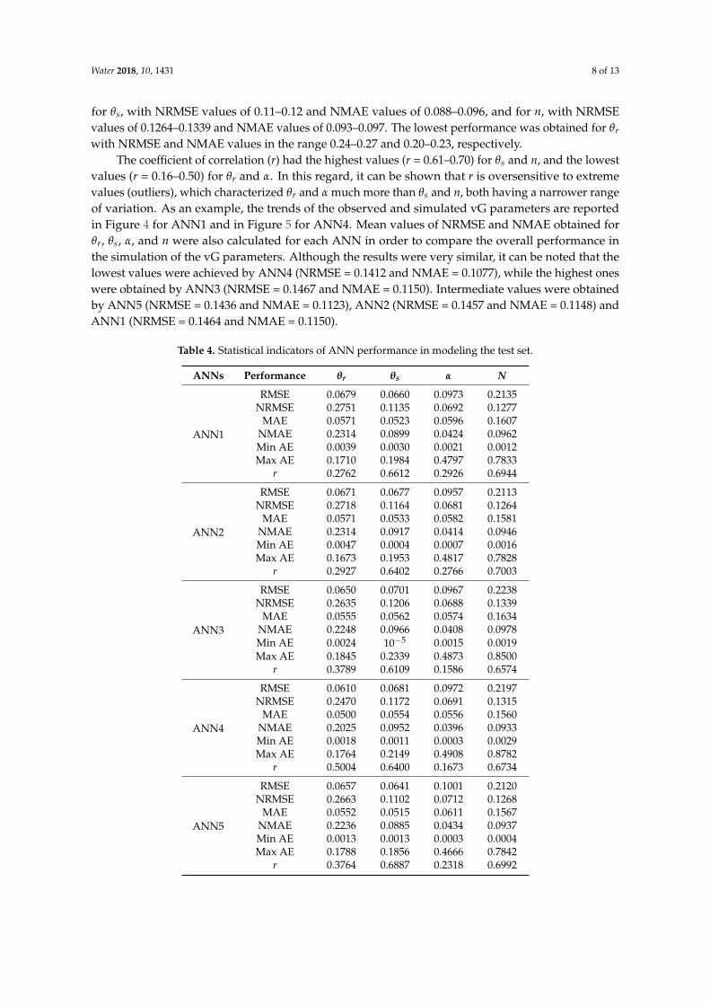
for θs, with NRMSE values of 0.11–0.12 and NMAE values of 0.088–0.096, and for n, with NRMSEvalues of 0.1264–0.1339 and NMAE values of 0.093–0.097. The lowest performance was obtained for θr

with NRMSE and NMAE values in the range 0.24–0.27 and 0.20–0.23, respectively.The coefficient of correlation (r) had the highest values (r = 0.61–0.70) for θs and n, and the lowest

values (r = 0.16–0.50) for θr and α. In this regard, it can be shown that r is oversensitive to extremevalues (outliers), which characterized θr and α much more than θs and n, both having a narrower rangeof variation. As an example, the trends of the observed and simulated vG parameters are reportedin Figure 4 for ANN1 and in Figure 5 for ANN4. Mean values of NRMSE and NMAE obtained forθr, θs, α, and n were also calculated for each ANN in order to compare the overall performance inthe simulation of the vG parameters. Although the results were very similar, it can be noted that thelowest values were achieved by ANN4 (NRMSE = 0.1412 and NMAE = 0.1077), while the highest oneswere obtained by ANN3 (NRMSE = 0.1467 and NMAE = 0.1150). Intermediate values were obtainedby ANN5 (NRMSE = 0.1436 and NMAE = 0.1123), ANN2 (NRMSE = 0.1457 and NMAE = 0.1148) andANN1 (NRMSE = 0.1464 and NMAE = 0.1150).

Table 4. Statistical indicators of ANN performance in modeling the test set.

ANNs Performance θr θs α N

ANN1

RMSE 0.0679 0.0660 0.0973 0.2135NRMSE 0.2751 0.1135 0.0692 0.1277

MAE 0.0571 0.0523 0.0596 0.1607NMAE 0.2314 0.0899 0.0424 0.0962Min AE 0.0039 0.0030 0.0021 0.0012Max AE 0.1710 0.1984 0.4797 0.7833

r 0.2762 0.6612 0.2926 0.6944

ANN2

RMSE 0.0671 0.0677 0.0957 0.2113NRMSE 0.2718 0.1164 0.0681 0.1264

MAE 0.0571 0.0533 0.0582 0.1581NMAE 0.2314 0.0917 0.0414 0.0946Min AE 0.0047 0.0004 0.0007 0.0016Max AE 0.1673 0.1953 0.4817 0.7828

r 0.2927 0.6402 0.2766 0.7003

ANN3

RMSE 0.0650 0.0701 0.0967 0.2238NRMSE 0.2635 0.1206 0.0688 0.1339

MAE 0.0555 0.0562 0.0574 0.1634NMAE 0.2248 0.0966 0.0408 0.0978Min AE 0.0024 10−5 0.0015 0.0019Max AE 0.1845 0.2339 0.4873 0.8500

r 0.3789 0.6109 0.1586 0.6574

ANN4

RMSE 0.0610 0.0681 0.0972 0.2197NRMSE 0.2470 0.1172 0.0691 0.1315

MAE 0.0500 0.0554 0.0556 0.1560NMAE 0.2025 0.0952 0.0396 0.0933Min AE 0.0018 0.0011 0.0003 0.0029Max AE 0.1764 0.2149 0.4908 0.8782

r 0.5004 0.6400 0.1673 0.6734

ANN5

RMSE 0.0657 0.0641 0.1001 0.2120NRMSE 0.2663 0.1102 0.0712 0.1268

MAE 0.0552 0.0515 0.0611 0.1567NMAE 0.2236 0.0885 0.0434 0.0937Min AE 0.0013 0.0013 0.0003 0.0004Max AE 0.1788 0.1856 0.4666 0.7842

r 0.3764 0.6887 0.2318 0.6992

Water 2018, 10, 1431 9 of 13Water 2018, 10, x FOR PEER REVIEW 9 of 13

Figure 4. Observed and simulated vG parameters obtained by ANN1.

Figure 5. Observed and simulated vG parameters obtained by ANN4.

Table 5 reports the MAE and RMSE values for the estimated soil water retention data obtained

with the considered ANNs. The calculations refer to the test dataset that comprises 90 soils. It is worth

noting that ANNs that made use of four input data generally performed better than those that used

three input data. Specifically, the minimum MAE was obtained by ANN5, while ANN4 had the

minimum RMSE. Less satisfactory results were obtained by ANN1, whereas the highest values of

both MAE and RMSE were obtained with ANN3.

Table 5. Statistical indicators of ANN performance in simulating water retention.

Network MAE RMSE r2

ANN1 0.030 0.074 0.75

ANN2 0.032 0.076 0.74

ANN3 0.032 0.089 0.65

ANN4 0.026 0.069 0.79

ANN5 0.016 0.074 0.72

Table 6 reports the results of the AIC test performed to evaluate the efficiency of the five ANNs

in simulating both the vG parameters and the water retention data. Equation (4) was used for the first

case, with the number of test samples equal to 90, while Equation (3) was applied in the second case,

0

0.1

0.2

0.3

0.4

0.5

0.6

0.7

0.8

0.0

0.5

1.0

1.5

2.0

2.5

3.0

1 9 17 25 33 41 49 57 65 73 81 89

a

q, n

Dataset

ϑr observed ϑr simulated ϑs observed ϑs simulated

n observed n simulated α observed α simulated

0

0.1

0.2

0.3

0.4

0.5

0.6

0.7

0.8

0.0

0.5

1.0

1.5

2.0

2.5

3.0

1 9 17 25 33 41 49 57 65 73 81 89

a

q, n

Dataset

ϑr observed ϑr simulated ϑs observed ϑs simulated

n observed n simulated α observed α simulated

Figure 4. Observed and simulated vG parameters obtained by ANN1.

Water 2018, 10, x FOR PEER REVIEW 9 of 13

Figure 4. Observed and simulated vG parameters obtained by ANN1.

Figure 5. Observed and simulated vG parameters obtained by ANN4.

Table 5 reports the MAE and RMSE values for the estimated soil water retention data obtained

with the considered ANNs. The calculations refer to the test dataset that comprises 90 soils. It is worth

noting that ANNs that made use of four input data generally performed better than those that used

three input data. Specifically, the minimum MAE was obtained by ANN5, while ANN4 had the

minimum RMSE. Less satisfactory results were obtained by ANN1, whereas the highest values of

both MAE and RMSE were obtained with ANN3.

Table 5. Statistical indicators of ANN performance in simulating water retention.

Network MAE RMSE r2

ANN1 0.030 0.074 0.75

ANN2 0.032 0.076 0.74

ANN3 0.032 0.089 0.65

ANN4 0.026 0.069 0.79

ANN5 0.016 0.074 0.72

Table 6 reports the results of the AIC test performed to evaluate the efficiency of the five ANNs

in simulating both the vG parameters and the water retention data. Equation (4) was used for the first

case, with the number of test samples equal to 90, while Equation (3) was applied in the second case,

0

0.1

0.2

0.3

0.4

0.5

0.6

0.7

0.8

0.0

0.5

1.0

1.5

2.0

2.5

3.0

1 9 17 25 33 41 49 57 65 73 81 89

a

q, n

Dataset

ϑr observed ϑr simulated ϑs observed ϑs simulated

n observed n simulated α observed α simulated

0

0.1

0.2

0.3

0.4

0.5

0.6

0.7

0.8

0.0

0.5

1.0

1.5

2.0

2.5

3.0

1 9 17 25 33 41 49 57 65 73 81 89

a

q, n

Dataset

ϑr observed ϑr simulated ϑs observed ϑs simulated

n observed n simulated α observed α simulated

Figure 5. Observed and simulated vG parameters obtained by ANN4.

Table 5 reports the MAE and RMSE values for the estimated soil water retention data obtainedwith the considered ANNs. The calculations refer to the test dataset that comprises 90 soils. It isworth noting that ANNs that made use of four input data generally performed better than those thatused three input data. Specifically, the minimum MAE was obtained by ANN5, while ANN4 had theminimum RMSE. Less satisfactory results were obtained by ANN1, whereas the highest values of bothMAE and RMSE were obtained with ANN3.

Table 5. Statistical indicators of ANN performance in simulating water retention.

Network MAE RMSE r2

ANN1 0.030 0.074 0.75ANN2 0.032 0.076 0.74ANN3 0.032 0.089 0.65ANN4 0.026 0.069 0.79ANN5 0.016 0.074 0.72

Table 6 reports the results of the AIC test performed to evaluate the efficiency of the five ANNs insimulating both the vG parameters and the water retention data. Equation (4) was used for the firstcase, with the number of test samples equal to 90, while Equation (3) was applied in the second case,

Water 2018, 10, 1431 10 of 13

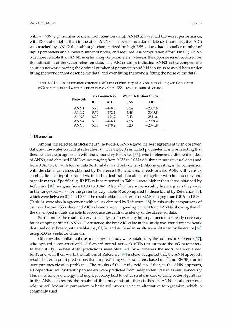
with n = 939 (e.g., number of measured retention data). ANN3 always had the worst performance,with RSS quite higher than in the other ANNs. The best simulation efficiency (more negative AIC)was reached by ANN2 that, although characterized by high RSS values, had a smaller number ofinput parameters and a lower number of nodes, and required less computation effort. Finally, ANN5was more reliable than ANN4 in estimating vG parameters, whereas the opposite result occurred forthe estimation of the water retention data. The AIC criterion indicated ANN2 as the compromisesolution network, having the optimal number of parameters and hidden units to avoid both underfitting (network cannot describe the data) and over fitting (network is fitting the noise of the data).

Table 6. Akaike’s information criterion (AIC) test of efficiency of ANNs in modeling van Genuchten(vG) parameters and water retention curve values. RSS—residual sum of square.

NetworkvG Parameters Water Retention Curve

RSS AIC RSS AIC

ANN1 5.75 −468.3 5.14 −2887.8ANN2 5.74 −472.4 5.48 −3095.5ANN3 6.23 −464.9 7.43 −2811.6ANN4 5.88 −466.4 4.56 −2999.4ANN5 5.63 −470.2 5.23 −2871.8

4. Discussion

Among the selected artificial neural networks, ANN4 gave the best agreement with observeddata, and the water content at saturation, θs, was the best simulated parameter. It is worth noting thatthese results are in agreement with those found by Reference [35], who implemented different modelsof ANNs, and obtained RMSE values ranging from 0.053 to 0.085 with three inputs (textural data) andfrom 0.048 to 0.08 with four inputs (textural data and bulk density). Also interesting is the comparisonwith the statistical values obtained by Reference [18], who used a feed-forward ANN with variouscombinations of input parameters, including textural data alone or together with bulk density andorganic matter. Specifically, RMSE values reported in Table 6 were higher than those obtained byReference [18], ranging from 0.039 to 0.047. Also, r2 values were sensibly higher, given they werein the range 0.65−0.79 for the present study (Table 5) as compared to those found by Reference [18],which were between 0.12 and 0.34. The results obtained in terms of MAE, ranging from 0.016 and 0.032(Table 6), were also in agreement with values obtained by Reference [18]. In this study, comparisons ofestimated mean RSS values and AIC indicators were in good agreement for all ANNs, showing that allthe developed models are able to reproduce the central tendency of the observed data.

Furthermore, the results deserve an analysis of how many input parameters are really necessaryfor developing artificial ANNs. For instance, the best AIC value in this study was found for a networkthat used only three input variables, i.e., Cl, Sa, and ρb. Similar results were obtained by Reference [36]using RSS as a selector criterion.

Other results similar to those of the present study were obtained by the authors of Reference [37],who applied a constructive feed-forward neural network (CFN) to estimate the vG parameters.In their study, the best ANN predictions were obtained for α, whereas the worst were obtainedfor θs and n. In their work, the authors of Reference [37] instead suggested that the ANN approachresults better in point predictions than in predicting vG parameters, based on r2 and RMSE, due toover-parameterization problems. The results of this study evidenced that, in the ANN approach,all dependent soil hydraulic parameters were predicted from independent variables simultaneously.This saves time and energy, and might probably lead to better results in case of using better algorithmsin the ANN. Therefore, the results of the study indicate that studies on ANN should continuerelating soil hydraulic parameters to basic soil properties as an alternative to regression, which iscommonly used.

Water 2018, 10, 1431 11 of 13

Therefore, starting from a large and variable database of soil properties, the results obtainedherein assessed the ability of the ANN approach in mimicking the real soil water retention curvethrough an accurate and reliable estimation of vG parameters.

Unlike other parametric regression techniques, which define relationships of soil propertiesusing mathematical functions, the well-defined ability of the ANN technique in interpreting theinput/output relationship of complex soil water systems [38,39] explains its adequate performance inboth the training and validation phases.

From the results obtained in this study, it is possible to highlight that ANN approachescan determine complementary insights to support decision-making in the irrigation context ofSicilian agriculture.

5. Conclusions

The prediction of soil water retention characteristics is basically important for simulating soilwater fluxes in the root zone aimed at establishing irrigation scheduling, but also sustainability ofrain-fed agriculture. Knowledge of the soil water retention curve is also crucial in soil conservation,drought forecasting, and soil quality assessment. Artificial neural networks are flexible mathematicalstructures that are capable of identifying complex non-linear relationships among input and outputdatasets. The principal differences among the various types of ANNs are the arrangement of neuronsand the assessment of the weights and functions for inputs and neurons (training).

In this study, five ANN models were developed to estimate the vG parameters for simulatingagricultural soil water availability for crops. The performance and efficiency of the selected ANNswere evaluated using different statistical indicators. Results showed the good predictive capability ofthe trained ANNs with different inputs and hidden layers. Statistical indicators confirmed the highpredictive performance of ANNs with four input parameters (Cl, Sa, and Si fractions, and OC),two hidden nodes with 15 neurons each, four output nodes, and training cycles of minimum2000 epochs. In simulating soil water retention data, ANN4 resulted in a prediction accuracycharacterized by MAE = 0.026 and RMSE = 0.069.

The AIC efficiency criterion indicated that most efficient ANN model was trained with a relativelylow number of input nodes. This approach may be preferable for estimating soil water retentioncharacteristics to be used for agro-hydrological simulations at a regional scale. The most efficientANN can be used for soil mapping in areas with similar soil hydraulic and textural features withoutadditional field surveys. A large database of soil hydraulic data for Sicily was used in this study,suggesting that the implemented ANNs could be considered a valuable general approach to plan cropproduction, optimize water resources management, and select environmental protection operations.

Author Contributions: The authors contributed with equal effort to the realization of the study.

Funding: This research was funded by a grant of the Sicilian Region (Progetto Metodologie innovative per lacaratterizzazione idraulica e la valutazione della qualità fisica dei suoli siciliani—CISS-2011-13).

Conflicts of Interest: The authors declare no conflicts of interest. The funders had no role in the design of thestudy; in the collection, analyses, or interpretation of data; in the writing of the manuscript, and in the decision topublish the results.

References

1. Wösten, J.H.M.; Lilly, A.; Nemes, A.; Le Bas, C. Development and use of a database of hydraulic propertiesof European soils. Geoderma 1999, 90, 169–185. [CrossRef]

2. De Melo Moreira, T.; Pedrollo, O.C. Artificial neural networks for estimating soil water retention curve usingfitted and measured data. Appl. Environ. Soil Sci. 2015, 2015, 535216. [CrossRef]

3. Jana, R.B.; Mohanty, B.P.; Springer, E.P. Multiscale Pedotransfer Functions for Soil Water Retention.Vadose Zone J. 2007, 6, 868–878. [CrossRef]

4. Zacharias, S.; Wessolek, G. Excluding Organic Matter Content from Pedotransfer Predictors of Soil WaterRetention. Soil Sci. Soc. Am. J. 2007, 71, 43–50. [CrossRef]

Water 2018, 10, 1431 12 of 13

5. Van Genuchten, M.T. A closed form equation for predicting the hydraulic conductivity of unsaturated soils.Soil Sci. Soc. Am. J. 1980, 44, 892–898. [CrossRef]

6. Dexter, A.R.; Czyz, E.A.; Richard, G.; Reszkowska, A. A user-friendly water retention function that takesaccount of the textural and structural pore spaces in soil. Geoderma 2008, 143, 243–253. [CrossRef]

7. Wosten, J.H.M.; van Genuchten, M.T. Using texture and other soil properties to predict the unsaturated soilhydraulic functions. Soil Sci. Soc. Am. J. 1988, 52, 1762–1770. [CrossRef]

8. Schaap, M.G.; Bouten, W. Modeling water retention curves of sandy soils using neural networks.Water Resour. Res. 1996, 32, 3033–3040. [CrossRef]

9. Scheinost, A.C.; Sinowski, W.; Auerswald, K. Regionalization of soil water retention curves in a highlyvariable soilscape, I. Developing a new pedotransfer function. Geoderma 1997, 78, 129–143. [CrossRef]

10. Minasny, B.; McBratney, A.B.; Bristow, K.I. Comparison of different approaches to the development ofpedotransfer functions for water retention curves. Geoderma 1999, 93, 225–253. [CrossRef]

11. Wösten, J.H.M.; Pachepsky, Y.A.; Rawls, W.J. Pedotransfer functions: Bridging the gap between availablebasic soil data and missing soil hydraulic characteristics. J. Hydrol. 2001, 251, 123–150. [CrossRef]

12. Brooks, R.H.; Corey, A.T. Hydraulic properties of porous media and their relation to drainage design.Trans. ASAE 1964, 7, 0026–0028.

13. Campbell, G.S. A simple method for determining unsaturated hydraulic conductivity from moisture retentiondata. Soil Sci. 1974, 177, 311–314. [CrossRef]

14. Wang, G.; Zhanga, Y.; Yu, N. Prediction of soil water retention and available water of sandy soils usingpedotransfer functions. Procedia Eng. 2012, 37, 49–53. [CrossRef]

15. Pachepsky, Y.A.; Rawls, W.J. Accuracy and reliability of pedotransfer functions as affected by grouping soils.Soil Sci. Soc. Am. J. 1999, 63, 1748–1757. [CrossRef]

16. Haghverdi, A.; Öztürk, H.S.; Cornelis, W.M. Revisiting the pseudo continuous pedotransfer function concept:Impact of data quality and data mining method. Geoderma 2014, 226, 31–38. [CrossRef]

17. Mukhlisin, M.; El-Shafie, A.; Taha, M.R. Regularized versus non-regularized neural network model forprediction of saturated soil-water content on weathered granite soil formation. Neural Comput. Appl. 2012,21, 543–553. [CrossRef]

18. Patil, N.G.; Pal, D.K.; Mandal, C.; Mandal, D.K. Soil water retention characteristics of vertisols andpedotransfer functions based on nearest neighbour and neural networks approaches to estimate AWC.J. Irrig. Drain. Eng. 2012, 138, 177–184. [CrossRef]

19. Minasny, B.; Hartemink, A.E. Predicting soil properties in the tropics. Earth-Sci. Rev. 2011, 106, 52–62.[CrossRef]

20. Patil, N.G.; Singh, S.K. Pedotransfer functions for estimating soil hydraulic properties: A review. Pedosphere2016, 26, 417–430. [CrossRef]

21. Brooks, R.H.; Corey, A.T. Properties of porous media affecting fluid flow. J. Irrig. Drain. Div. 1966, 92, 61–90.22. Aiello, R.; Bagarello, V.; Barbagallo, S.; Consoli, S.; Di Prima, S.; Giordano, G.; Iovino, M. An assessment

of the Beerkan method for determining the hydraulic properties of a sandy loam soil. Geoderma 2014,235–236, 300–307. [CrossRef]

23. Antinoro, C.; Bagarello, V.; Ferro, V.; Giordano, G.; Iovino, M. A simplified approach to estimate waterretention for Sicilian soils by the Arya–Paris model. Geoderma 2014, 213, 226–234. [CrossRef]

24. Bagarello, V.; Iovino, M. Testing the BEST procedure to estimate the soil water retention curve. Geoderma2012, 187, 67–76. [CrossRef]

25. Gee, G.W.; Bauder, J.W. Particle-size analysis1. In Methods of Soil Analysis: Part 1—Physical and MineralogicalMethods, (Methodsofsoilan1); American Society of Agronomy-Soil Science Society of America: Madison,WI, USA, 1986; pp. 383–411.

26. Shirazi, M.A.; Boersma, L. A Unifying Quantitative Analysis of Soil Texture 1. Soil Sci. Soc. Am. J. 1984,48, 142–147. [CrossRef]

27. Nelson, D.W.; Sommers, L.E. Total carbon, organic carbon, and organic matter. In Methods of Soil AnalysisPart 3—Chemical Methods, (Methodsofsoilan3); American Society of Agronomy-Soil Science Society of America:Madison, WI, USA, 1996; pp. 961–1010.

28. Van Genuchten, M.V.; Leij, F.J.; Yates, S.R. The RETC Code for Quantifying the Hydraulic Functions of UnsaturatedSoils; Research Report n. EPA/600/2-91/065; U.S. Salinity Laboratory, USDA-ARS: Riverside, CA, USA,1991; 93p.

Water 2018, 10, 1431 13 of 13

29. D’Emilio, A.; Mazzarella, R.; Porto, S.M.C.; Cascone, G. Neural networks for predicting greenhouse thermalregimes during soil solarization. Trans. ASABE 2012, 55, 1093–1103. [CrossRef]

30. Akaike, H. A new look at the statistical model identification. IEEE Trans. Autom. Control 1974, 19, 716–723.[CrossRef]

31. Panchal, G.; Ganatra, A.; Kosta, Y.P.; Panchal, D. Searching most efficient neural network architecture usingAkaike’s information criterion (AIC). Int. J. Comput. Appl. 2010, 1, 41–44. [CrossRef]

32. Chang, C.H.; Wu, S.J.; Hsu, C.T.; Shen, J.C.; Lien, H.C. An evaluation framework for identifying the optimalraingauge network based on spatiotemporal variation in quantitative precipitation estimation. Hydrol. Res.2017, 48, 77–98. [CrossRef]

33. Laio, F.; Di Baldassarre, G.; Montanari, A. Model selection techniques for the frequency analysis ofhydrological extremes. Water Res. Res. 2009, 45, 1–11. [CrossRef]

34. Rossel, R.V.; Behrens, T. Using data mining to model and interpret soil diffuse reflectance spectra. Geoderma2010, 158, 46–54. [CrossRef]

35. Minasny, B.; McBratney, A.B. The neuro-m method for fitting neural network parametric pedotransferfunctions. Soil Sci. Soc. Am. J. 2002, 66, 352–361. [CrossRef]

36. Jain, S.K.; Singh, V.P.; van Genuchten, M.T. Analysis of soil water retention data using artificial neuralnetworks. J. Hydrol. Eng. 2004, 9, 415–420. [CrossRef]

37. Merdun, H.; Cinar, O.; Meral, R.; Apan, M. Comparison of artificial neural network and regressionpedotransfer functions for prediction of soil water retention and saturated hydraulic conductivity.Soil Tillage Res. 2006, 90, 108–116. [CrossRef]

38. Pachepsky, Y.; Schaap, M.G. Data mining and exploration techniques. Dev. Soil Sci. 2004, 30, 21–32.39. Haghverdi, A.; Cornelis, W.M.; Ghahraman, B. A pseudo-continuous neural network approach for

developing water retention pedotransfer functions with limited data. J. Hydrol. 2012, 442, 46–54. [CrossRef]

© 2018 by the authors. Licensee MDPI, Basel, Switzerland. This article is an open accessarticle distributed under the terms and conditions of the Creative Commons Attribution(CC BY) license (http://creativecommons.org/licenses/by/4.0/).