Artificial Neural Networks

ARTIFICIAL NEURAL NETWORKS

Modeling Nature’s Solution

Neural Networks 2

Want to model approach after those found in natureBest learner in nature?

Brain

8/29/03

Want machines to learn

Neural Networks 3

How Do Brain’s Learn? Vast networks of cells called

neurons Human ~100 billion neurons Each neuron estimated to have

~1,000 connections to other neurons

Known as synaptic connections ~100 trillion synapses

8/29/03

Neural Networks 4

Pathways for Electrical Signals A neuron receives input from the axons of other

neurons Dendrites form a web of possible input locations When the incoming potentials reach a critical

level the neuron fires exciting neurons downstream

8/29/03

Neural Networks 5

Donald Hebb 1949

Psychologist: proposed that classical conditioning (Pavlovian) is possible because of individual neuron properties

Proposed a mechanism for learning in biological neurons

8/29/03

Neural Networks 68/29/03

Hebb’s Rule

Let us assume that the persistence or repetition of a reverberatory activity (or "trace") tends to induce lasting cellular changes that add to its stability.… When an axon of cell A is near enough to excite a cell B and repeatedly or persistently takes part in firing it, some growth process or metabolic change takes place in one or both cells such that A's efficiency, as one of the cells firing B, is increased.

Neural Networks 7

Repetitive Reinforcement Some synaptic

connections fire more easily over time Less resistance Form synaptic pathways

Some form “callouses” and are more resistant to firing

8/29/03

Neural Networks 8

LearningIn a very real sense, learning can be boiled down to the process of determining the appropriate resistances between the vast network of axon to dendrite connections in the brain

8/29/03

Neural Networks 9

1940’s Warren McCulloch and

Walter Pitts Showed that networks of

artificial neurons could, in principle, compute any arithmetic or logical function

8/29/03

Warren McCulloch

Walter Pitts

Neural Networks 10

Abstraction Neuron: like an electrical circuit with

multiple inputs and a single output (though it can branch out to multiple locations)

8/29/03

ΣAnd some threshold

AxonDen

drit

es

Neural Networks 11

Learning Learning becomes a matter of

discovering the appropriate resistance values

8/29/03

ΣAnd some threshold

AxonDen

drit

es

Neural Networks 12

Computationally Resistors become weights Linear combination

8/29/03

ΣW1

W2

W3

Wn

W0

.

.

.

inpu

ts

Bias

fTransfer Function

Neural Networks 13

1950’s Interest sored Bernard Widrow and

Ted Hoff introduced a new learning rule

Widrow-Hoff (still in use today)

Used in the simple Perceptron neural network

8/29/03

Neural Networks 14

1960 Frank Rosenblatt Cornell University Created the Perceptron

Computer Perceptrons were simulated

on an IBM 704

First computer that could learn new skills by trial and error

8/29/03

IEEE’s Frank Rosenblatt Award, for "outstanding contributions to the advancement of the design, practice, techniques or theory in biologically and linguistically motivated computational paradigms including but not limited to neural networks, connectionist systems, evolutionary computation, fuzzy systems, and hybrid intelligent systems in which these paradigms are contained."

Neural Networks 15

Perceptron As usual, each training instance used to

adjust weights

8/29/03

Σ

W1

W2

W3

Wn

W0

.

.

.

inpu

ts

Bias

f

Transfer Function

Class Training Data

Neural Networks 16

Learning rule

t is target (class) o is output (output of perceptron)

8/29/03

∆𝑤 𝑖=𝜂 ∑𝑑∈𝐷

(𝑡𝑑−𝑜𝑑)𝑥𝑖𝑑

Neural Networks 17

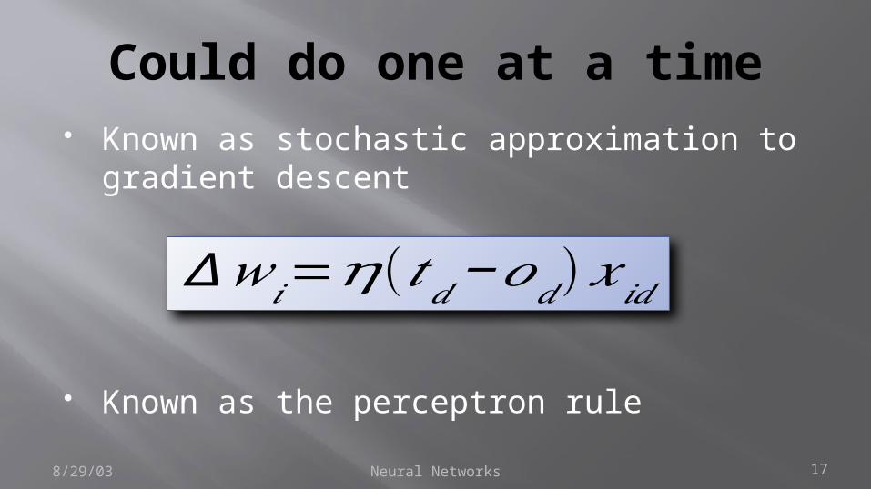
Could do one at a time Known as stochastic approximation to

gradient descent

Known as the perceptron rule8/29/03

∆𝑤 𝑖=𝜂 (𝑡𝑑−𝑜𝑑)𝑥 𝑖𝑑

Neural Networks 18

Transfer Function Output (remember: target – output) Example: binary class—0 or 1 hardlim(n)

If n < 0 return 0 Otherwise return 1

8/29/03

Σ

W1

W2

W3

Wn

W0

.

.

.

inpu

ts

Bias

f

Transfer Function

Neural Networks 19

Example Decision boundary Red

Class 0 Green

Class 1

8/29/03

0 2 4 6 8

02

46

810

X

Y

W = [0.195, -0.065, 0.0186]

Neural Networks 20

0 2 4 6 8

02

46

810

X

Y

Classification Decision boundary Linear combination Hardlim(n)

If n < 0 return 0 Otherwise return 1

8/29/03

For plotting purposes

Neural Networks 21

Algorithm Gradient-Descent(training_examples,η)

Each training example is a pair of the form where is the vector of input values, and is the target output value, η is the learning rate (e.g. .05)

Initialize each to some small random value Until the termination condition is met, DO

Initialize each to zero For each in training_examples, DO

Input the instance to the unit and compute the output o For each linear unit weight , DO

For each linear unit weight , DO

8/29/03

∆𝑤 𝑖=𝜂 (𝑡𝑑−𝑜𝑑)𝑥 𝑖𝑑

Neural Networks 22

0 2 4 6 8

02

46

8

X

Y

Implementation in R

8/29/03

Initialize each _ to some small random value𝑤 𝑖Until the termination condition is met, DO

Initialize each ∆ _ to zero𝑤 𝑖For each ⟨ ⃗, ⟩ in training_examples, DO𝑥 𝑡

Input the instance ⃗ to the unit and compute the 𝑥output oFor each linear unit weight _ , DO𝑤 𝑖

∆𝑤_ ← ( − ) _𝑖 𝜂 𝑡 𝑜 𝑥 𝑖For each linear unit weight _ , DO𝑤 𝑖𝑤_ ← _ +∆ _𝑖 𝑤 𝑖 𝑤 𝑖

eta = .001deltaW = rep(0,numDims + 1)errorCount = 1epoch = 0while(errorCount>0){ errorCount = 0 for (idx in c(1:dim(trData)[1])){#for each tr inst deltaW = 0*deltaW #init delta w to zero input = c(1,trData[idx,1:2]) #input is xy of tr output = hardlim(sum(w*input)) #run thru perceptron target = trData[idx,3] if(output != target){ errorCount=errorCount + 1 } #calc delta w deltaW = eta*(target - output)*input w = w + deltaW } if(epoch %% 100 == 0){ abline(c(-w[1]/w[3],-w[2]/w[3]),col="yellow") }}

Neural Networks 23

0 2 4 6 8

02

46

8

X

Y

When did it stop? Stopping condition?

8/29/03

How well will it classify future instances?

Neural Networks 24

What if not linearly separable

Use hardlim to train (t-o), not residual

Not minimizing square differences

8/29/03

1 2 3 4 5 6 7

01

23

45

6

X

Y

Neural Networks 25

Serious Limitations Book “Perceptrons”

published in 1969 (Marvin Minsky and Seymour Papert) Publicized inherent limitations

of ANN’s Couldn’t solve a simple XOR

problem8/29/03

Seymour Papert

Marvin Minsky

Neural Networks 26

Artificial Neural Networks Dead? Many were influenced by

Minsky and Papert Mass exodus from the field For a decade, research in ANNs

lay mostly dormant

8/29/03

Neural Networks 27

Far From Antagonistic Minsky and Papert developed the

“Society of the Mind” theory Intelligence could be a product of the

interaction of non-intelligent parts Quote from Arthur C. Clarke,

2001: A Space Odyssey “Minsky and Good had shown how neural

networks could be generated automatically—self replicated… Artificial brains could be grown by a process strikingly analogous to the development of a human brain. “

8/29/03

Neural Networks 28

The AI winter In fact, the effect was field wide More likely a combination of hype

generated unreasonable expectations and several high profile AI failures

8/29/03

Speech recognitionAutomatic translatorsExpert systems

Neural Networks 29

Not completely dead Funding was down But, during this time…

ANNs shown to be usable as memory (Kohonen networks)

Stephen Grossberg developed self-organizing networks (SOMs)

8/29/03

Neural Networks 30

1980s More accessible

computing Revitalization Renaissance

8/29/03

Neural Networks 31

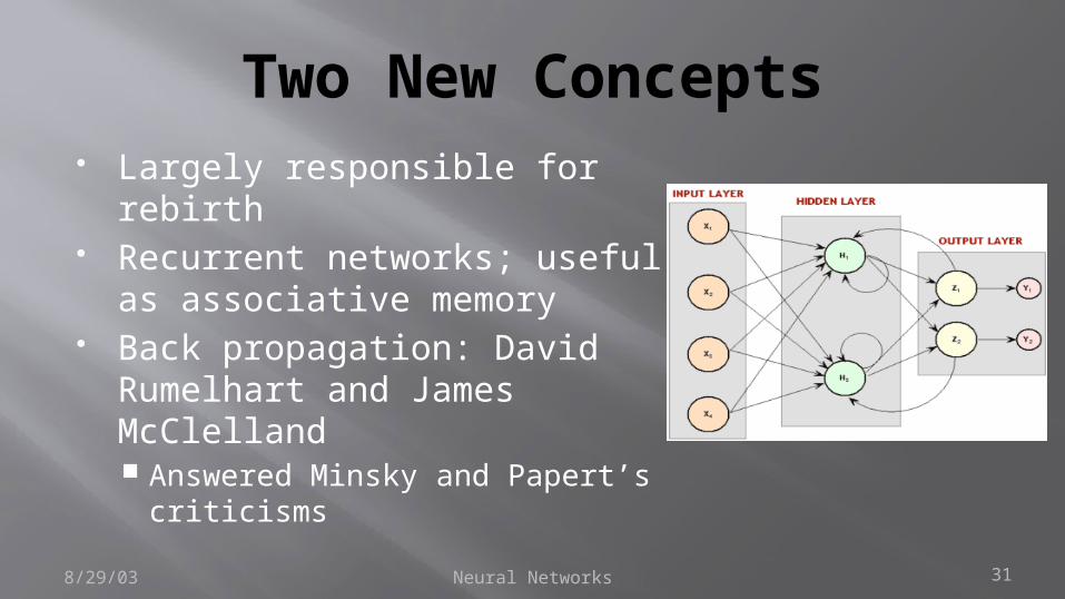
Two New Concepts Largely responsible for

rebirth Recurrent networks; useful as

associative memory Back propagation: David

Rumelhart and James McClelland Answered Minsky and Papert’s

criticisms8/29/03

Neural Networks 32

Multilayer Networks

8/29/03

Σ fww

w

...Σ fw

w

w

...

Σ fww

w

...Σ fw

w

w

...

x1x2

xm

... Σ fww

w

...Σ fw

w

w

...

Σ fww

w

...

Σ fww

w

...

Σ fww

w

...

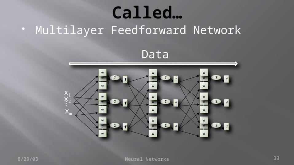
Input Units Hidden layer Output Units

Neural Networks 33

Called… Multilayer Feedforward Network

8/29/03

Data

Σ fww

w

...Σ fw

w

w

...

Σ fww

w

...Σ fw

w

w

...

x1x2

xm

... Σ fww

w

...Σ fw

w

w

...

Σ fww

w

...

Σ fww

w

...

Σ fww

w

...

Neural Networks 34

Adjusting Weights… Must be done in the context of the

current layer’s input and output But what is the “target” value for a given

layer?

8/29/03

Σ f

w

...w

w

Base these weight adjustments on these output values

Neural Networks 35

Instead of… Working with target values, can work with

error values of the node ahead

8/29/03

• Output branches to several downstream nodes (albeit a particular input of that node)

• If we start at the output end, we know how far off the mark it is (its error)

Σ f

w

...w

w

Neural Networks 36

Non-output nodes Look at the “errors“ of the units ahead

instead of target values

8/29/03

Σ fw

w

w

...Σ fw

w

w

...

Error based on target and output (t-o)

Error based on the summation of the errors of the units to which it is tied

Neural Networks 37

Backpropagation of Error Backpropagation Learning Algorithm

8/29/03

Σ fw

w

w

...Σ f

w

w

w

...

Σ fw

w

w

...Σ f

w

w

w

...

x1

x2

xm

... Σ fw

w

w

...Σ f

w

w

w

...

Σ fw

w

w

...

Σ fw

w

w

...

Σ fw

w

w

...

Data

Error

Neural Networks 38

Error Calculations Original gradient descent

Partial differentiation of the overall error between a predicted line and target values

Residuals—regression

8/29/03

-10 -5 0 5

-10

-50

510

X

Y

∆𝑤 𝑖=𝜂 ∑𝑑∈𝐷

(𝑡 𝑑−𝑜𝑑 )𝑥𝑖𝑑

Target, the Y of the training data

Output, the calculated Y given Xi and the current values in the weight vector

Neural Networks 39

But… The perceptron rule switched to a

stochastic approximation And it was no longer, strictly speaking,

based upon gradient descent Hardlim non-differentiable

8/29/03

∆𝑤 𝑖=𝜂 (𝑡𝑑−𝑜𝑑)𝑥 𝑖𝑑 Σ

W1

W2

W3

Wn

W0

.

.

.

inpu

ts

Bias

f

Transfer Function

Neural Networks 40

In order… …to return to a

mathematically rigorous solution

Switched transfer functions

Sigmoid Can determine

instantaneous slopes8/29/03

Binary (Logistic) Sigmoid Function

ey bs 1

1

k

bs(k)1

0-5 5

Neural Networks 41

Delta weights Derivation

8/29/03

Where is the error on training example d, summed over all output units in the network

Outputs is the set of output units in the network, is the target value of the unit k for training example d, and is the output of unit k given training example d

Neural Networks 42

Stochastic gradient descent rule Some terms

8/29/03

the ith input to unit j the weight associated with the ith input to unit j (the weighted sum of inputs for unit j) the output computed by unit j the target output for unit j the sigmoid function the set of units in the final layer of the network the set of units whose immediate inputs include the output of unit j

Neural Networks 43

Derivation

8/29/03

Chain rule (weight can influence the rest of the network only through ) can influence the network only through

First term

Neural Networks 44

Derivation

8/29/03

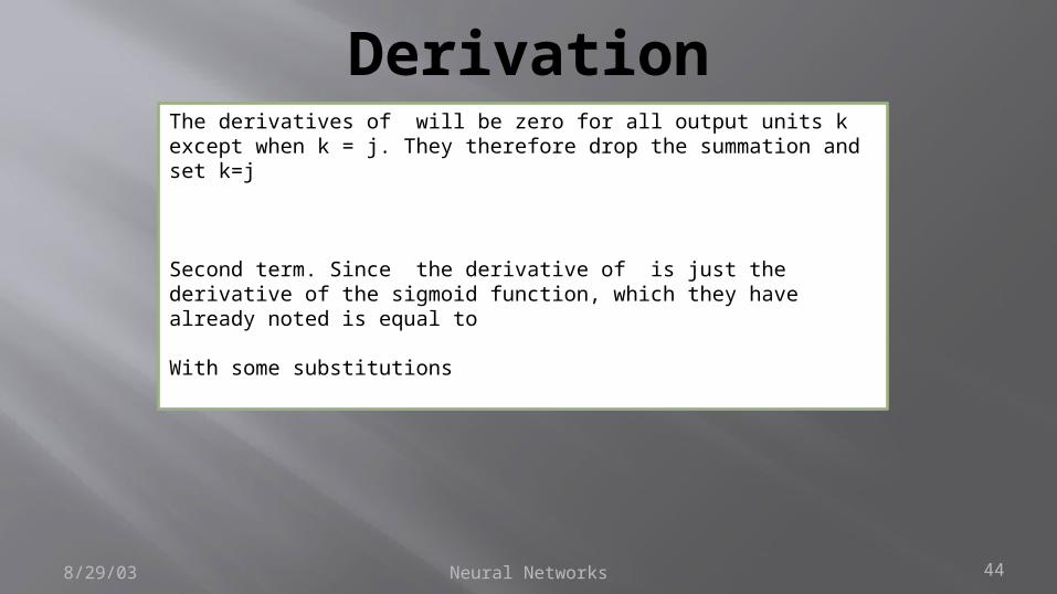
The derivatives of will be zero for all output units k except when k = j. They therefore drop the summation and set k=jSecond term. Since the derivative of is just the derivative of the sigmoid function, which they have already noted is equal to

With some substitutions

Neural Networks 45

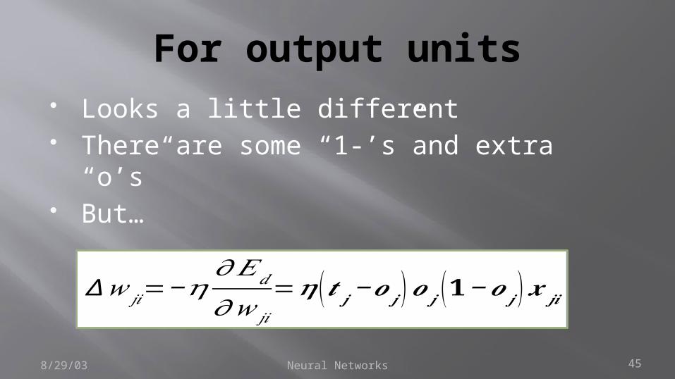
For output units Looks a little different There are some “1-’s”and extra “o’s” But…

8/29/03

∆𝑤 𝑗𝑖=−𝜂𝜕𝐸𝑑

𝜕𝑤 𝑗𝑖=𝜼 (𝒕 𝒋−𝒐 𝒋 )𝒐 𝒋 (𝟏−𝒐 𝒋 ) 𝒙 𝒋𝒊

Neural Networks 46

Hidden Units We are interested in the error associated

with a hidden unit

8/29/03

Error associated with a unit: Will designate as (the negative sign useful for direction of change computations)

Neural Networks 47

Derivation: Hidden Units

8/29/03

can influence the network only through the units in downstream j

Neural Networks 48

For Hidden Units Learning rate times error from connected

units ahead times the current input

8/29/03

And finally

Rearrange some terms and use to denote , they present: Backpropagation

Neural Networks 49

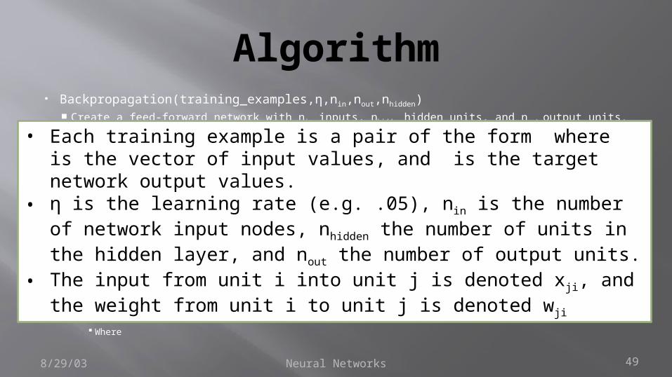
Algorithm Backpropagation(training_examples,η,nin,nout,nhidden)

Create a feed-forward network with nin inputs, nhidden hidden units, and nout output units. Initialize all network weights to some small random value (e.g. between -.05 and .05) Until the termination condition is met, DO

For each in training_examples, DO Propagate the input forward through the network: Input the instance to the unit and compute the output ou of every unit u in the network Propagate the errors backward through the network: For each network output unit k, calculate its error term δk

For each hidden unit h, calculate its error term δh

Where wkh is the weight in the next layer (k) to which oh is connected

Update each network weight wji

Where

8/29/03

• Each training example is a pair of the form where is the vector of input values, and is the target network output values.

• η is the learning rate (e.g. .05), nin is the number of network input nodes, nhidden the number of units in the hidden layer, and nout the number of output units.

• The input from unit i into unit j is denoted xji, and the weight from unit i to unit j is denoted wji

Neural Networks 50

Simple example

8/29/03

output

ΣW1

W01

net o or xinput ΣW1

W01

net o or xΣW1

W01

net

Sigmoid(.1) = 0.5249792

(1*.05+0.5249792*.05)= 0.07624896

0.519053(1*.05+1*.05)=0.1

(1*.05+ 0.519053*.05) = 0.07595265

0.518979

x=1,t=0

Assume all weights begin at .05Let’s feedforward

Neural Networks 51

Simple example

8/29/03

ΣW1

W01


W01

net o or x ΣW1

W01

netoutput

x=1,t=0

Assume all weights begin at .05

Node Errors

0.518979

)0.519053) 0.5249792

Neural Networks 52

Simple example

8/29/03

x=1,t=0

Assume all weights begin at .05Delta Weights

𝛿𝑜𝑢𝑡=−0.1295578

𝛿𝑜𝑢𝑡=−0.001617121

0.52497920.519053

𝛿𝑜𝑢𝑡=−2.016356 𝑒−05

∆𝑤 𝑗𝑖=−0.000129 6∆𝑤 𝑗𝑖=−1.617121 2𝑒−06∆𝑤 𝑗𝑖=−2.016356𝑒−08

ΣW1

W01


W01

net o or x ΣW1

W01

netoutput

Neural Networks 53

Less simple example 2 layers

8/29/03

x=1, t=0,0

Assume all weights begin at .05, also assume eta is .05

Let’s feedforward

Sigmoid(.1) = 0.5249792

(1*.05+0.5249792*.05+0.5249792*.05)= 0.1024979

0.5256(1*.05+1*.05)=0.1(1*.05 + 0.5256*.05 + 0.5256*.05) = 0.10256

0.52562

input

output

ΣW1

W01

net o or xΣW1

W01

net o or xΣW1

W01

net output

ΣW1

W01

net o or xΣ

W1

W01

net o or xΣ

W1

W01

netW1

W1

W1

W1

Neural Networks 54

Less simple example

8/29/03

x=1,t=0,0

Assume all weights begin at .05Node Errors

0.5256176

)

0.5256) 0.5249792

input

output

ΣW1

W01

net o or xΣW1

W01

net o or xΣW1

W01

net output

ΣW1

W01

net o or xΣ

W1

W01

net o or xΣ

W1

W01

netW1

W1

W1

W1

Neural Networks 55

Less simple example

8/29/03

x=1,t=0,0

𝛿𝑜𝑢𝑡=−0.131059𝛿𝑜𝑢𝑡=−0.00326 8

0.5249792 0.5256

𝛿𝑜𝑢𝑡=−8.149349𝑒−05

∆𝑤 𝑗𝑖=−0.00655297∆𝑤 𝑗𝑖=−0.00016339∆𝑤 𝑗𝑖=−4.074674𝑒−06

input

output

ΣW1

W01

net o or xΣW1

W01

net o or xΣW1

W01

net output

ΣW1

W01

net o or xΣ

W1

W01

net o or xΣ

W1

W01

netW1

W1

W1

W1

Neural Networks 56

Another

8/29/03

WhWh

ΣW1

W01

net

𝛿=−0.133

𝛿=−0.13 3

𝛿=0.115

W2

W3

𝑜=0.539

Wh

WhWhWh

WhWhWh

𝑤 h𝑘 =0.040

𝑤 h𝑘 =0.054

𝑤 h𝑘 =0.05 6

0.629

0.628

0.620

Neural Networks 57

My Implementation Started with a vector holding the number

of neurons at each level

8/29/03

Σ fw

w

w

...Σ f

w

w

w

Σ fw

w

w

Σ fw

w

w

...

x1

x2

xm

... Σ fw

w

w

...Σ f

w

w

w

Σ fw

w

w

Σ fw

w

w

Σ fw

w

w

3 3 3

Neural Networks 58

Object Oriented Network Neuron

8/29/03

Network Vector with counts for layersArray of arrays of neuronsNumber of inputs

FunctionsInitializeFeedforwardBackprop

Neuron Layer idNode id (within layer)Vector of weightsVector of current inputsCurrent outputDelta valueEta (η)

FunctionsFeedforwardSigmoidcalcOutDeltacalcInDeltaupdateWeights

Neural Networks 59

When initialize

Pass vector Eta (η)

Build array of arrays of neurons When instantiate each neuron

How know number of weights ? How about input layer

(how many weights?)8/29/03

Σ fw

w

w

...Σ f

w

w

w

Σ fw

w

w

Σ fw

w

w

...

x1x2

xm

... Σ fw

w

w

...Σ f

w

w

w

Σ fw

w

w

Σ fw

w

w

Σ fw

w

w

Neuron Layer idNode id (within layer)Vector of weightsVector of current inputsCurrent outputDelta valueEta

FunctionsFeedforwardSigmoidcalcOutDeltacalcInDeltaupdateWeights

Neural Networks 60

Network feedforward function Invoke feedforward on each neuron

8/29/03

Network level FeedForwardPass in inputsConcatenate one to the vector (for bias)For each layer

If layer >0 change inputs to prev layer outsFor each neuron in layer

Set inputsInvoke feedForward on neuron

Neuron level FeedForwardLinear combo with inputs and weightsSigmoid to update output

Neural Networks 61

Calculate deltas Pseudo code

8/29/03

At Network level invoke calcDeltasFor each node in output layer calcOutDeltaFor each layer (backwards from output layer)

For each node in layer calcInDeltaAt node level

calcOutDeltaPass in targetsFor each output node

Calculate deltaStore in node

calcInDeltaPass in vectors of forward delta’s and forward weightsForeach node calc deltaStore in node

Neural Networks 62

Calculate delta weights Have everything we need

8/29/03

At Network levelFor each layer

For each node update weightsAt node level

Have delta of node and inputs already storedCalculate updated weights

Neural Networks 63

With…

Iris data 3,3,3

Took hundreds of epochs to see any change in accuracy

But then quickly dove to 4 or 5 errors

8/29/03

Sepal Length Sepal Width Petal Length Petal Width Species5.1 3.5 1.4 0.2 setosa4.9 3.0 1.4 0.2 setosa4.7 3.2 1.3 0.2 setosa


Example: ALVINN Drives 70 mph on highways In traffic

Carnegie Mellon


Local Minima

Only guaranteed to converge toward some local minimum

Usually not a problem Every weight in a network

corresponds to a dimension in a very high dimensional search space (error surface)

A local minimum in one may not be a local minimum in the rest

The more dimensions the more “escape routes”


Weights initialized near zero

Early steps will represent a very smooth function that is approximately linear

Once the weights have reach plateaus generally close enough to the global minimum

Reasons: Sigmoid Function

k

bs(k)1

0-5 5


Descends a different error surface for each training example

Reasons: Stochastic Gradient Descent


Add a momentum term

Roll past local minima

A Possible Solution


Momentum

Perhaps most common modification to backprop Alpha is between 0 and 1

To right of “+” known as momentum term Keeps the ball rolling through small local minima

∆𝑤 𝑗𝑖 (𝑛)=𝜂𝛿 𝑗 𝑥 𝑗𝑖+𝛼 ∆𝑤 𝑗𝑖 (𝑛−1 )


Train multiple networks (starting with random weights). If achieve different solutions probably local minima.

Multiple Runs

Σf

w

w

w

...

Σf

w

w

w

Σf

w

w

w

Σf

w

w

w

...

x1x2

xm

... Σf

w

w

w

...

Σf

w

w

w

Σf

w

w

w

Σf

w

w

w

Σf

w

w

w

Σf

w

w

w

...

Σf

w

w

w

Σf

w

w

w

Σf

w

w

w

...

x1x2

xm

... Σf

w

w

w

...

Σf

w

w

w

Σf

w

w

w

Σf

w

w

w

Σf

w

w

w

Σf

w

w

w

...

Σf

w

w

w

Σf

w

w

w

Σf

w

w

w

...

x1x2

xm

... Σf

w

w

w

...

Σf

w

w

w

Σf

w

w

w

Σf

w

w

w

Σf

w

w

w

Σf

w

w

w

...

Σf

w

w

w

Σf

w

w

w

Σf

w

w

w

...

x1x2

xm

... Σf

w

w

w

...

Σf

w

w

w

Σf

w

w

w

Σf

w

w

w

Σf

w

w

w

Σf

w

w

w

...

Σf

w

w

w

Σf

w

w

w

Σf

w

w

w

...

x1x2

xm

... Σf

w

w

w

...

Σf

w

w

w

Σf

w

w

w

Σf

w

w

w

Σf

w

w

w

Neural Networks 71

Name Relation Icon

Hard Limit a=0 n<0a=1 n≥0

Symmetrical Hard Limit a=-1 n<0a=+1 n≥0

Linear a=n

Saturating Lineara=0 n<0a=n 0 ≤ n ≤ 1a=+1 n>0

Symmetric Saturating Lineara=-1 n<-1a=n -1 ≤ n ≤ +1a=+1 n>1

Log-Sigmoid

Hyperbolic Tangent Sigmoid

Positive Linear a=0 n<0a=n n≥0

Competitive a=1 max neurona=0 all other

8/29/03

Transfer Functions

C


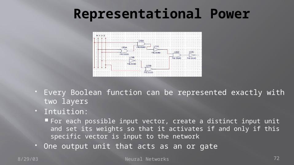
Representational Power

Every Boolean function can be represented exactly with two layers

Intuition: For each possible input vector, create a distinct input unit and set its

weights so that it activates if and only if this specific vector is input to the network

One output unit that acts as an or gate


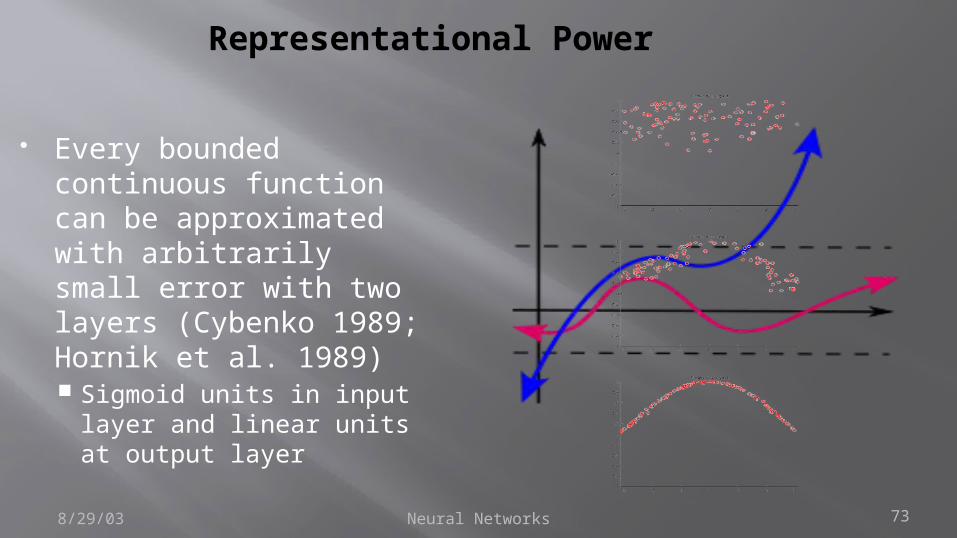
Every bounded continuous function can be approximated with arbitrarily small error with two layers (Cybenko 1989; Hornik et al. 1989) Sigmoid units in input

layer and linear units at output layer



Any function can be approximated with three layers (Cybenko 1988) Sigmoid in input and hidden layer,

linear units output Proof involves showing that any

function can be approximated by a linear combination of many localized functions and then showing that two layers of sigmoid units are sufficient to produce good local approximations.


Neural Networks 75

Every weight in a network corresponds to a dimension in a high dimensional search space (error surface)

Hypothesis space is continuous How about for

Decision trees Candidate elimination KNN Bayesian

W


8/29/03

Neural Networks 76

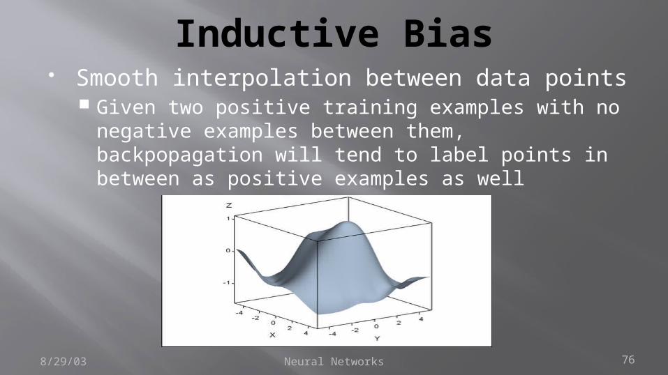
Inductive Bias Smooth interpolation between data points

Given two positive training examples with no negative examples between them, backpopagation will tend to label points in between as positive examples as well

8/29/03


Hidden Layer Getting an intuition about what the hidden

layers buy us Intermediate representation


Translation If you were going to represent 8 different

classes?

1 0 00 0 10 1 01 1 10 0 00 1 11 0 11 1 0


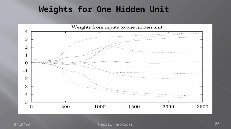
Hidden Unit Encoding Outputs as train


Weights for One Hidden Unit


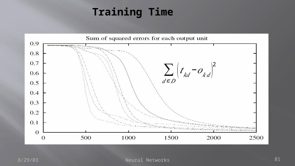
Training Time

∑𝑑∈𝐷

( 𝑡𝑘𝑑−𝑜𝑘𝑑 )2

Neural Networks 82

Susceptible to Overfitting? If network is complex enough can it achieve

perfect classification of training data? Remember: any function can be approximated

with arbitrarily small error with three layers

8/29/03

Memorize?𝐸 (�⃗� )=12 ∑𝑑∈𝐷

∑𝑘∈𝑜𝑢𝑡𝑝𝑢𝑡𝑠

(𝑡𝑘𝑑−𝑜𝑘𝑑 )2

Neural Networks 83

Susceptible

Weights begin as small random values As begin to learn some grow Over time complexity of the learned decision surface

increases Fits noise in the training data

Or unrepresentative characteristics of the particular training sample

8/29/03

Large Weights Overfitting

Neural Networks 84

Weight Decay Decrease each weight by some small factor during

each iteration Penalty that corresponds to the total magnitude of the

network weights The usual penalty is the sum of squared weights times

a decay constant.

8/29/03

Penalty termYields a weight update rule identical to backpropagation rule except that each weight is multiplied by the constant:

Neural Networks 85

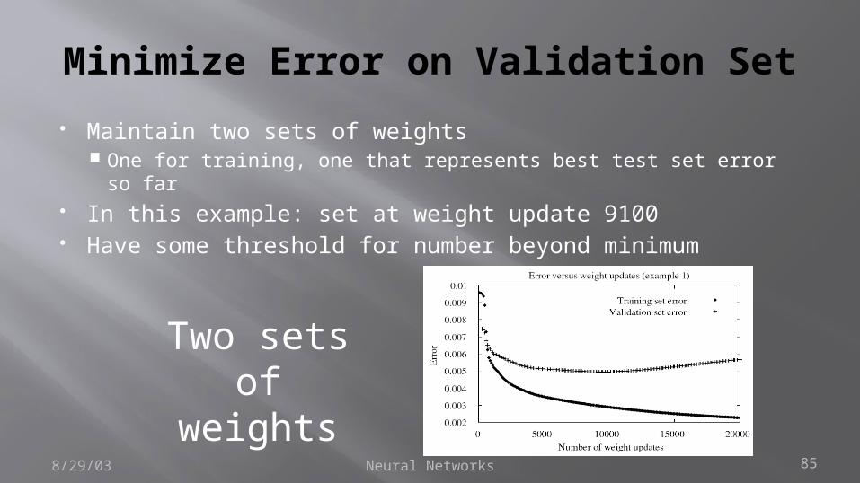
Minimize Error on Validation Set Maintain two sets of weights

One for training, one that represents best test set error so far In this example: set at weight update 9100 Have some threshold for number beyond minimum

8/29/03

Two sets of

weights


If K-fold

Determine best stopping generation (using validation set) in each fold

Average these Train on entire set

but stop at average best


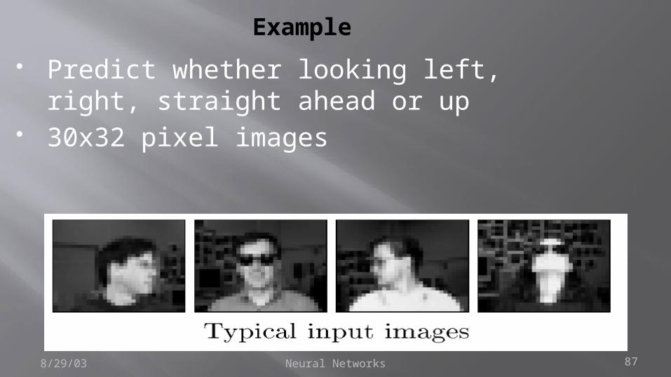
Example Predict whether looking left, right,

straight ahead or up 30x32 pixel images


Architecture?

There are 4 classes How many input nodes? Authors went with 2 layer

960 pixels 3 input nodes Why three?

How many output nodes? Authors went with 4


Parameters Learning rate of 0.3 Momentum of 0.3 Used .9 and .1 as targets

If 1 and 0 then weights could grow without bound Learned weights

Black: large negative White: large positive


Order—Trends Up to now order assumed unimportant In fact usually randomly shuffle training data What if some information were stored in the data

leading up to the current datum?

Streaming data like stock market Predict stock price

given a progression of economic indicators


Recurrent Networks

A component of the current input comes from a previous input

No longer acyclic Example: Elman Σ fw

w

w...

Σ fww

w

Σ fww

w

Σ fww

w...

x1x2

xm

... Σ fww

w...

Σ fww

w

Σ fww

w

Σ fww

w

Σ fww

w

wdelay

wdelay

wdelay


How Train

Unrolling network Calculate deltas

(errors) by considering all downstream deltas

One will be own previous delta (and weight)

Σ fww

w...

Σ fww

w

Σ fww

w

Σ fww

w...

x1x2

xm

... Σ fww

w...

Σ fww

w

Σ fww

w

Σ fww

w

Σ fww

w

wdelay

wdelay

wdelay


Hairpin Turn Prediction Protein Structure


Hairpin Turn Prediction Predict occurrences of four turns in a row Data from NCBI

1 DVSFRLSGAD PRSYGMFIKD LRNALPFREK VYNIPLLLPS VSGAGRYLLM EEEE TT HHHHHHHHHH HHHHS BS E ETTEEEE S GGGGEEEE

51 HLFNYDGKTI TVAVDVTNVY IMGYLADTTS YFFNEPAAEL ASQYVFRDAR EEE TTS EE EEEEETTTTE E EEEETTEE EE SSHHHHH HHTTS TT S

101 RKITLPYSGN YERLQIAAGK PREKIPIGLP ALDSAISTLL HYDSTAAAGA EEEE SS SS HHHHHHHHTS GGGSEESHH HHHHHHHHHT S HHHHHHH

151 LLVLIQTTAE AARFKYIEQQ IQERAYRDEV PSLATISLEN SWSGLSKQIQ HHHHHHHTHH HHHBHHHHHH HHHTSSS EE HHHHHHHH HTHHHHHHHH

201 LAQGNNGIFR TPIVLVDNKG NRVQITNVTS KVVTSNIQLL LNTRNI HHTTTTTB S S EEEE TTS SEEEE BTTT HHHHHTB B TTTT


Representation 4-mers Integer for each amino acid Include some Chou-Fasman parameters

4, 20, 16, 14, 0.147, 0.048, 0.125, 0.065, 020, 16, 14, 2, 0.062, 0.139, 0.065, 0.085, 016, 14, 2, 11, 0.120, 0.041, 0.099, 0.070, 014, 2, 11, 16, 0.059, 0.106, 0.036, 0.106, 0 2, 11, 16, 8, 0.070, 0.025, 0.125, 0.152, 011, 16, 8, 1, 0.061, 0.139, 0.190, 0.058, 016, 8, 1, 4, 0.120, 0.085, 0.035, 0.081, 0 8, 1, 4, 15, 0.102, 0.076, 0.179, 0.068, 0 1, 4, 15, 2, 0.060, 0.110, 0.034, 0.085, 0 4, 15, 2, 16, 0.147, 0.301, 0.099, 0.106, 0


Biased … Achieved excellent results (too good to be true) Very few positives in the data Only correctly predicted 50% of the positives How improve?


Improvements

Bootstrap Balance dataset

Went to 12-mer More context

Went to a recurrent network

Achieved results as good as best in class

Recurrence provided most dramatic improvement


Remember Hebb’s Rule

Let us assume that the persistence or repetition of a reverberatory activity (or "trace") tends to induce lasting cellular changes that add to its stability.… When an axon of cell A is near enough to excite a cell B and repeatedly or persistently takes part in firing it, some growth process or metabolic change takes place in one or both cells such that A's efficiency, as one of the cells firing B, is increased.


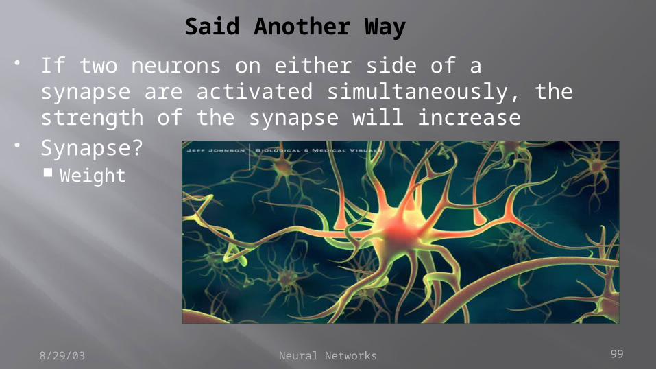
Said Another Way If two neurons on either side of a synapse are

activated simultaneously, the strength of the synapse will increase

Synapse? Weight


Interpretation could be that if a positive input produces a positive output then the weights should increase

A possible implementation

Where t and p are vectors of target and input values respectively

Hebbian Learning

𝑊𝑛𝑒𝑤=𝑊𝑜𝑙𝑑+𝑡 �⃗�𝑇

Hebb learning Rule

Neural Networks 101

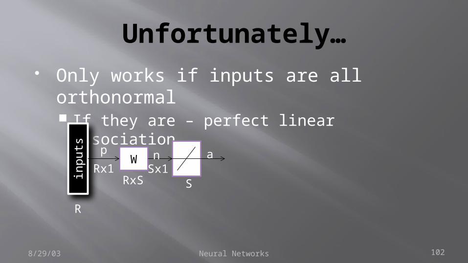
Weights Handled a Little Differently No longer one weight per input and

summed A row per input, a column per output

8/29/03

a Wp=

p1 t1{ , } p2 t2{ , } pQ tQ{ , } Training Set:

ai w ijp jj 1=

R

=

Linear Associator

(Function Remembering)

inpu

ts

W

R

Rx1 Sx1S

anp

RxS

Neural Networks 102

Unfortunately… Only works if inputs are all orthonormal

If they are – perfect linear association

8/29/03

inpu

ts

W

R

Rx1 Sx1S

anp

RxS


Can use a trick—pseudoinverseIf not…

Was New methodWhere T is a matrix of all targets and P+ is the pseudoinverse of the matrix of all inputs

Neural Networks 104

Only Works… If number of training instances is smaller

than the number of dimensions in the input

The important thing…

8/29/03

Perfect recall—a form of memory

Neural Networks 105

Another application… Autoassociative memory Wikipedia: memories that enable one to

retrieve a piece of data from only a tiny sample of itself.

Note the output

8/29/03in

puts

W

R

Rx1 Rx1R

anp

RxR


Example

6x5 character represented as a 30 dimensional vectorp1 1– 1 1 1 1 1– 1 1– 1– 1– 1– 1 1 1– 1 1–

T=

W p1p1T p2p2

T p3p3T

+ +=

inpu

ts

W

R

Rx1 Rx1R

anp

RxR


Weights 30x30 “memory” of the characters If feed one of the characters in, will get

the same thing out

inpu

ts

W

R

Rx1 Rx1Rx1

anp

RxR


The cool thing… Can “recognize” similar patterns

Noisy Patterns (7 pixels)


Like layered memory Intuition

p1 = c(-1,1,1)p2 = c(1,-1,-1)

W1 = p1%*%t(p1)W2 = p2%*%t(p2)

W=W1+W2

> W [,1] [,2] [,3][1,] 2 -2 -2[2,] -2 2 2[3,] -2 2 2> W1 [,1] [,2] [,3][1,] 1 -1 -1[2,] -1 1 1[3,] -1 1 1> W2 [,1] [,2] [,3][1,] 1 -1 -1[2,] -1 1 1[3,] -1 1 1

> p1%*%W [,1] [,2] [,3][1,] -6 6 6> > p2%*%W [,1] [,2] [,3][1,] 6 -6 -6

Neural Networks 110

Associative Memory The zero example

8/29/03

p1=c(-1,1,1,1,1,-1,1,-1,-1,-1,-1,1,1,-1,-1,-1,-1,1,1,-1,-1,-1,-1,1,-1,1,1,1,1,-1)W = p1%*%t(p1)p1%*%W [,1] [,2] [,3] [,4] [,5] [,6] [,7] [,8] [,9] [,10] [,11] [,12] [,13] [,14] [,15] [,16][1,] -30 30 30 30 30 -30 30 -30 -30 -30 -30 30 30 -30 -30 -30 [,17] [,18] [,19] [,20] [,21] [,22] [,23] [,24] [,25] [,26] [,27] [,28] [,29] [,30][1,] -30 30 30 -30 -30 -30 -30 30 -30 30 30 30 30 -30


Can cluster: Self Organizing Maps (SOM) Work has been done on self evolving

networks Learn the optimal number of nodes and layers

Neural Nets

Artificial Neural Networks

Documents

Transcript of Artificial Neural Networks