Artificial Intelligence Methods (G5BAIM) - Examination ...pszgxk/aim/2009/exam/2001-02.pdfArtificial...

Artificial Intelligence Methods (G5BAIM) - Examination

Question 1 a) Explain the difference between a genotypic representation and a phenotypic representation. Give an example of each.

(8) (b) Outline the similarities and differences between Genetic Algorithms and Evolutionary Strategies.

(8) (c) Describe the terms recency with respect to tabu search.

(4) (d) Outline the simulated annealing cooling schedule, describing the various components.

(5)

Graham Kendall


Question 2 a) Given the following parents, P1 and P2, and the template T P1 A B C D E F G H I J P2 E F J H B C I A D G T 1 0 1 1 0 0 0 1 0 1 Show how the following crossover operators work • uniform crossover • order-based crossover with regards to genetic algorithms

(8) Use this problem description for parts b to e. Assume we have the following function

f(x) = x3 - 60 * x2 + 900 * x +100 where x is constrained to 0..31. We wish to maximize f(x) (the optimal is x=10) Using a binary representation we can represent x using five binary digits. b) Given the following four chromosomes give the values for x and f(x).

Chromosome Binary String P1 11100 P2 01111 P3 10111 P4 00100

(2)

c) If P3 and P2 are chosen as parents and we apply one point crossover show the resulting children, C1 and C2. Use a crossover point of 1 (where 0 is to the very left of the chromosome) Do the same using P4 and P2 with a crossover point of 2 and create C3 and C4

(6) d) Calculate the value of x and f(x) for C1..C4.

(2) e) Assume the initial population was x={17, 21, 4 and 28}. Using one-point crossover, what is the probability of finding the optimal solution? Explain your reasons.

(7)

Graham Kendall


Question 3 (a) Show a simulated annealing algorithm

(7) (b) Define the acceptance function that is used by simulated annealing and describe the terms.

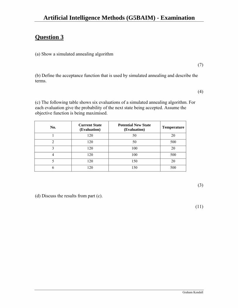
(4) (c) The following table shows six evaluations of a simulated annealing algorithm. For each evaluation give the probability of the next state being accepted. Assume the objective function is being maximised.

No. Current State (Evaluation)

Potential New State (Evaluation) Temperature

1 120 50 20 2 120 50 500 3 120 100 20 4 120 100 500 5 120 150 20 6 120 150 500

(3) (d) Discuss the results from part (c).

(11)

Graham Kendall


Question 4 a) Given the following problems, decide what type of optimisation technique, from those presented in the lectures, you would use? Justify your decision. In answering, describe your choice of representation and the operators that you would use.

i) Minimise a function that has n real variables. ii) The Travelling Salesman Problem iii) An artificial ant that has find a trail of food on a grid.

(18)

b) Suggest a problem that you would like to solve using one of the techniques we considered in the lectures. Again, describe the representation for the problem and the operators you would use. The problem you choose should not a toy problem. That is, it should not be so simple that the optimal solution can easily found using other methods.

(7)

Graham Kendall


Question 5 a) With reference to evolutionary strategies explain the difference between the comma and plus notation.

(7) b) With regards to evolutionary strategies, describe the Rechenberg “1/5 success rule”, discuss why it is used and possible parameters.

(10) c) With regard to evolutionary strategies what do you understand by the term self adaptation?

(8)

Graham Kendall


Graham Kendall

Question 6 a) Describe how ants are able to find the shortest path to a food source.

(4) b) Using the travelling salesman problem as an example, describe the following terms in relation to ant algorithms Visibility Evaporation Transition Probability

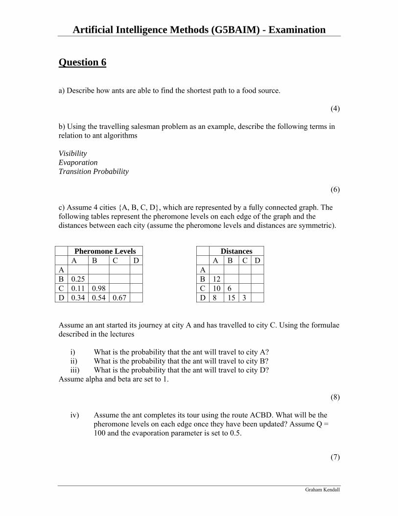
(6) c) Assume 4 cities {A, B, C, D}, which are represented by a fully connected graph. The following tables represent the pheromone levels on each edge of the graph and the distances between each city (assume the pheromone levels and distances are symmetric). Pheromone Levels Distances A B C D A B C DA A B 0.25 B 12 C 0.11 0.98 C 10 6 D 0.34 0.54 0.67 D 8 15 3 Assume an ant started its journey at city A and has travelled to city C. Using the formulae described in the lectures

i) What is the probability that the ant will travel to city A? ii) What is the probability that the ant will travel to city B? iii) What is the probability that the ant will travel to city D?

Assume alpha and beta are set to 1.

(8)

iv) Assume the ant completes its tour using the route ACBD. What will be the pheromone levels on each edge once they have been updated? Assume Q = 100 and the evaporation parameter is set to 0.5.

(7)


Model Answers

Graham Kendall


Question 1 – Model Answer This question, unlike the other question in this examination, covers a wide variety of topics. This is designed to give the student who has done general revision the opportunity to pick up some marks. a) Explain the difference between a genotypic representation and a phenotypic representation. Give an example of each. This was an underlying theme throughout the course, mainly through David Fogel videos. A genotypic representation is one where the underlying representation has to be decoded in order to determine the behaviour of the organisim.

2 marks An example could be a bit string, which represents a set of real numbers with the binary digits having to be decoded in order to determine the real numbers, which can then be evaluated by carrying out the relevant function.

2 marks The underlying representation for a phenotypic representation represents the problem in a natural way. The behaviour is expressed directly into the representation.

2 marks An example, could be a robot arm, where the coding is directly related to the movement of the arm. For example, move right, turn 21°, move up etc. etc.

2 marks (b) Outline the similarities and differences between Genetic Algorithms and Evolutionary Strategies. The differences, particularly in the early work include

ES’s were single population approaches, whereas genetic algorithms were always population based approaches.

Gentic Algorithms mainly used a binary representations and evolutionary strategies optimised real valued functions.

Genetic algorithms used crossover and mutation. Evolutionary strategies only used mutation.

Graham Kendall


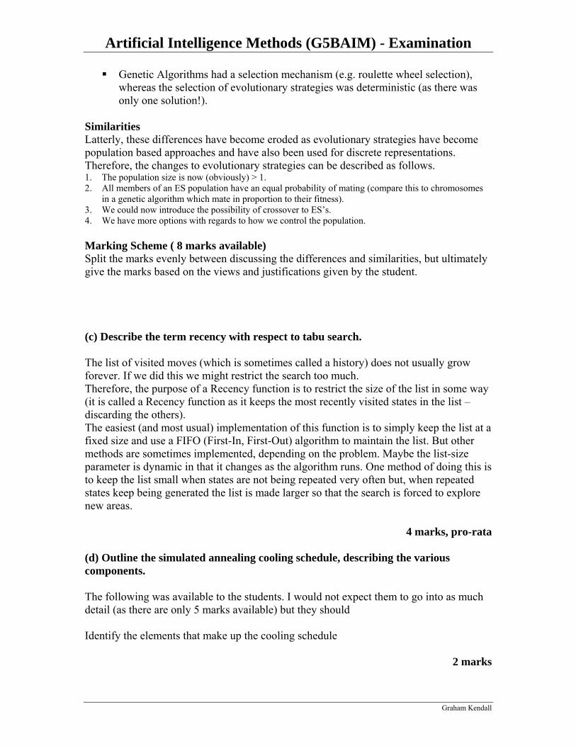
Genetic Algorithms had a selection mechanism (e.g. roulette wheel selection), whereas the selection of evolutionary strategies was deterministic (as there was only one solution!).

Similarities Latterly, these differences have become eroded as evolutionary strategies have become population based approaches and have also been used for discrete representations. Therefore, the changes to evolutionary strategies can be described as follows. 1. The population size is now (obviously) > 1. 2. All members of an ES population have an equal probability of mating (compare this to chromosomes

in a genetic algorithm which mate in proportion to their fitness). 3. We could now introduce the possibility of crossover to ES’s. 4. We have more options with regards to how we control the population. Marking Scheme ( 8 marks available) Split the marks evenly between discussing the differences and similarities, but ultimately give the marks based on the views and justifications given by the student. (c) Describe the term recency with respect to tabu search. The list of visited moves (which is sometimes called a history) does not usually grow forever. If we did this we might restrict the search too much. Therefore, the purpose of a Recency function is to restrict the size of the list in some way (it is called a Recency function as it keeps the most recently visited states in the list – discarding the others). The easiest (and most usual) implementation of this function is to simply keep the list at a fixed size and use a FIFO (First-In, First-Out) algorithm to maintain the list. But other methods are sometimes implemented, depending on the problem. Maybe the list-size parameter is dynamic in that it changes as the algorithm runs. One method of doing this is to keep the list small when states are not being repeated very often but, when repeated states keep being generated the list is made larger so that the search is forced to explore new areas.

4 marks, pro-rata (d) Outline the simulated annealing cooling schedule, describing the various components. The following was available to the students. I would not expect them to go into as much detail (as there are only 5 marks available) but they should Identify the elements that make up the cooling schedule

2 marks

Graham Kendall


Discuss the various elements

3 marks, pro-rata

The cooling schedule of a simulated annealing algorithm consists of four components. • Starting Temperature • Final Temperature • Temperature Decrement • Iterations at each temperature Starting Temperature The starting temperature must be hot enough to allow a move to almost any neighbourhood state. If this is not done then the ending solution will be the same (or very close) to the starting solution. Alternatively, we will simply implement a hill climbing algorithm. However, if the temperature starts at too high a value then the search can move to any neighbour and thus transform the search (at least in the early stages) into a random search. Effectively, the search will be random until the temperature is cool enough to start acting as a simulated annealing algorithm. The problem is finding the correct starting temperature. At present, there is no known method for finding a suitable starting temperature for a whole range of problems. Therefore, we need to consider other ways. If we know the maximum distance (cost function difference) between one neighbour and another then we can use this information to calculate a starting temperature. Another method, suggested in (Rayward-Smith, 1996), is to start with a very high temperature and cool it rapidly until about 60% of worst solutions are being accepted. This forms the real starting temperature and it can now be cooled more slowly. A similar idea, suggested in (Dowsland, 1995), is to rapidly heat the system until a certain proportion of worse solutions are accepted and then slow cooling can start. This can be seen to be similar to how physical annealing works in that the material is heated until it is liquid and then cooling begins (i.e. once the material is a liquid it is pointless carrying on heating it). Final Temperature It is usual to let the temperature decrease until it reaches zero. However, this can make the algorithm run for a lot longer, especially when a geometric cooling schedule is being used (see below). In practise, it is not necessary to let the temperature reach zero because as it approaches zero the chances of accepting a worse move are almost the same as the temperature being equal to zero. Therefore, the stopping criteria can either be a suitably low temperature or when the system is “frozen” at the current temperature (i.e. no better or worse moves are being accepted). Temperature Decrement Once we have our starting and stopping temperature we need to get from one to the other. That is, we need to decrement our temperature so that we eventually arrive at the stopping criterion. The way in which we decrement our temperature is critical to the success of the algorithm. Theory states that we should allow enough iterations at each temperature so that the system stabilises at that temperature. Unfortunately, theory also states that the number of iterations at each temperature to achieve this might be exponential to the problem size. As this is impractical we need to compromise. We can either do this by doing a large number of iterations at a few temperatures, a small number of iterations at many temperatures or a balance between the two. One way to decrement the temperature is a simple linear method. An alternative is a geometric decrement where

t = tα

Graham Kendall


where α < 1. Experience has shown that α should be between 0.8 and 0.99, with better results being found in the higher end of the range. Of course, the higher the value of α, the longer it will take to decrement the temperature to the stopping criterion. Iterations at each Temperature The final decision we have to make is how many iterations we make at each temperature. A constant number of iterations at each temperature is an obvious scheme. Another method, first suggested by (Lundy, 1986) is to only do one iteration at each temperature, but to decrease the temperature very slowly. The formula they use is

t = t/(1 + βt) where β is a suitably small value. I have entered this formula on a spreadsheet (available from the web site) so that you can play around with the parameters, if you are interested. An alternative is to dynamically change the number of iterations as the algorithm progresses. At lower temperatures it is important that a large number of iterations are done so that the local optimum can be fully explored. At higher temperatures, the number of iterations can be less.

Graham Kendall


Question 2 – Model Answer a) Given the following parents, P1 and P2, and the template T Uniform P1 A B C D E F G H I J P2 E F J H B C I A D G T 1 0 1 1 0 0 0 1 0 1 C1 A F C D B C I H D J C2 E B J H E F G A I G Order-Based P1 A B C D E F G H I J P2 E F J H B C I A D G T 1 0 1 1 0 0 0 1 0 1 C1 A E C D F B I H G J C2 E B J H C D F A I G

4 marks each b) Given the following four chromosomes give the values for x and f(x).

Chromosome Binary String x f(x) P1 11100 28 212 P2 01111 15 3475 P3 10111 23 1227 P4 00100 4 2804

2 marks (half mark each)

c) If P3 and P2 are chosen as parents and we apply one point crossover show the resulting children, C1 and C2. Use a crossover point of 1 (where 0 is on the very left of the chromosome) Do the same using P4 and P2 with a crossover point of 2 and create C3 and C4

Chromosome Binary String x f(x) C1 11111 31 131 C2 00111 7 3803 C3 00111 7 3803 C4 01100 12 3998

Graham Kendall


x and f(x) can be ignored for this question (see (d)).

6 marks (1.5 marks for each child they get correct) d) Calculate the value of x and f(x) for C1..C4. These are shown in the above table

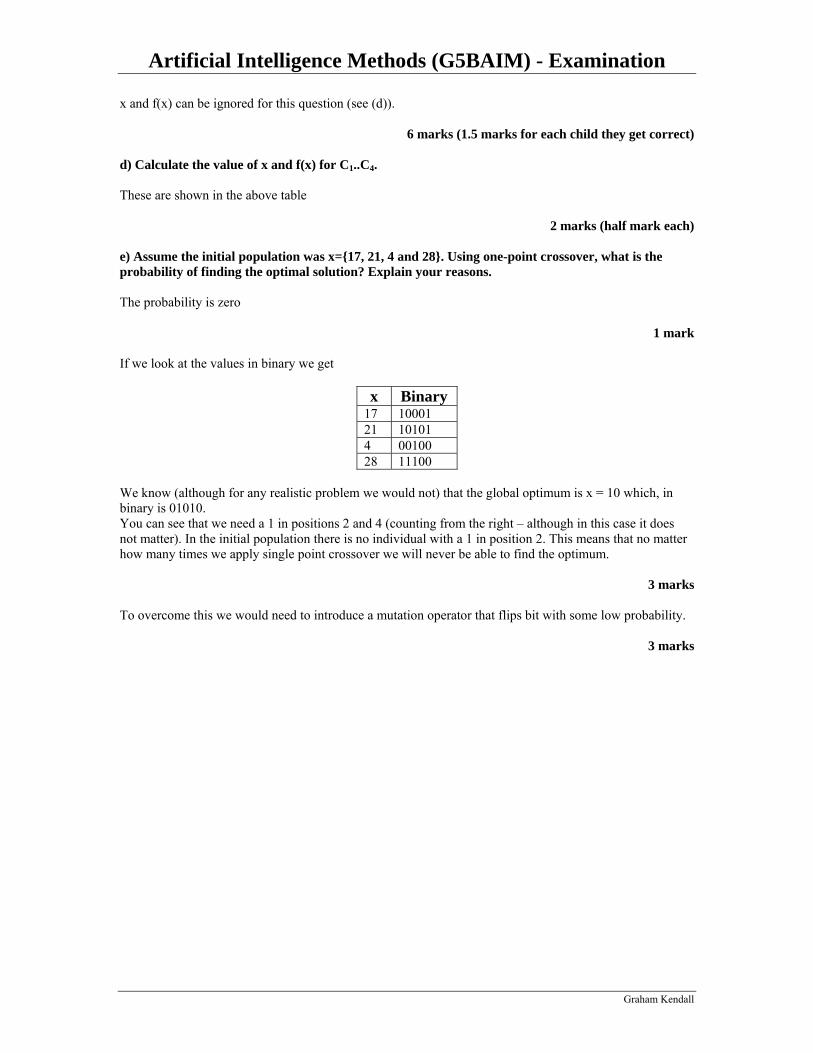
2 marks (half mark each) e) Assume the initial population was x={17, 21, 4 and 28}. Using one-point crossover, what is the probability of finding the optimal solution? Explain your reasons. The probability is zero

1 mark If we look at the values in binary we get

x Binary 17 10001 21 10101 4 00100 28 11100

We know (although for any realistic problem we would not) that the global optimum is x = 10 which, in binary is 01010. You can see that we need a 1 in positions 2 and 4 (counting from the right – although in this case it does not matter). In the initial population there is no individual with a 1 in position 2. This means that no matter how many times we apply single point crossover we will never be able to find the optimum.

3 marks To overcome this we would need to introduce a mutation operator that flips bit with some low probability.

3 marks

Graham Kendall


Question 3 – Model Answer (a) Show a simulated annealing algorithm This is the algorithm shown in the course textbook. Other algorithms may also be acceptable (bearing in mind that this lecture was given by a guest lecturer who may have presented the algorithm differently). Function SIMULATED-ANNEALING(Problem, Schedule) returns a solution state

Inputs : Problem, a problem Schedule, a mapping from time to temperature Local Variables : Current, a node

Next, a node T, a “temperature” controlling the probability of downward steps

Current = MAKE-NODE(INITIAL-STATE[Problem]) For t = 1 to ∞ do

T = Schedule[t] If T = 0 then return Current Next = a randomly selected successor of Current ΛE = VALUE[Next] – VALUE[Current] if ΛE > 0 then Current = Next else Current = Next only with probability exp(-ΛE/T)

Marks will also be given for showing a hill climbing algorithm (one that only accepts better neighbourhood moves) that has an acceptance criteria that accepts worse moves with some probability (that probability being exp(ΛE/T))

7 marks, pro-rata (b) Simulated Annealing Acceptance Function The accept function is given by

Probability of accepting a worse solution = exp(ΛE/T) Where ΛE is the change in the evaluation function and T is the current temperature The students might define it as follows IF proposed_neighbourhood_move is an improvement then

current_solution = proposed_neighbourhood_move ELSE

current_solution = proposed_neighbourhood_move with probability exp(ΛE/T) ENDIF

Graham Kendall


In fact, these two methods lead to the same thing as an improving move will have a probability > 1, but it would save a call to the exponential function. In awarding the marks, it is important that the student does state what the acceptance function (exp(ΛE/T)) is. I will be awarding half the marks just for stating this.

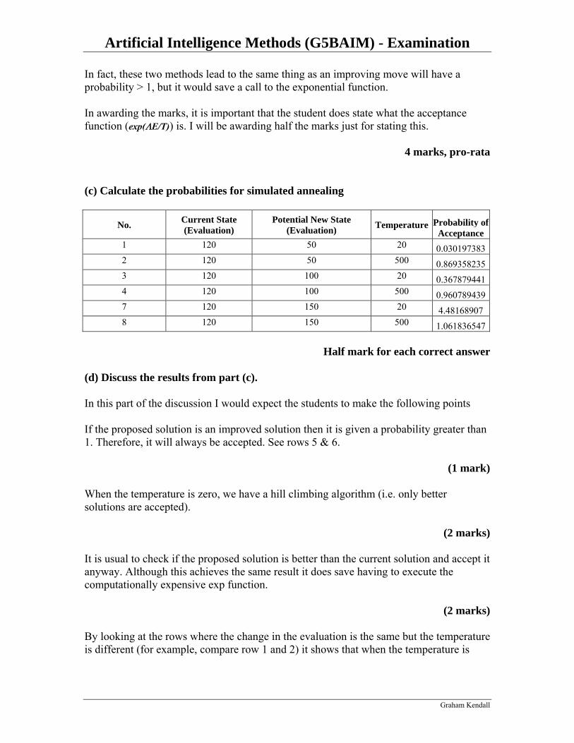
4 marks, pro-rata (c) Calculate the probabilities for simulated annealing

No. Current State (Evaluation)

Potential New State (Evaluation) Temperature Probability of

Acceptance 1 120 50 20 0.0301973832 120 50 500 0.8693582353 120 100 20 0.3678794414 120 100 500 0.9607894397 120 150 20 4.48168907 8 120 150 500 1.061836547

Half mark for each correct answer

(d) Discuss the results from part (c). In this part of the discussion I would expect the students to make the following points If the proposed solution is an improved solution then it is given a probability greater than 1. Therefore, it will always be accepted. See rows 5 & 6.

(1 mark) When the temperature is zero, we have a hill climbing algorithm (i.e. only better solutions are accepted).

(2 marks) It is usual to check if the proposed solution is better than the current solution and accept it anyway. Although this achieves the same result it does save having to execute the computationally expensive exp function.

(2 marks) By looking at the rows where the change in the evaluation is the same but the temperature is different (for example, compare row 1 and 2) it shows that when the temperature is

Graham Kendall


higher the probability of the worse solution being accepted is higher, even when the change in the evaluation function is the same.

(2 marks) When the temperature is the same, but the evaluations are different, there is a higher probability of choosing the better of the worse solutions (compare row 1 with row 3).

(1 mark) Another 3 discretionary marks to be awarded for any other points made by student, especially if it shows evidence of reading the literature. For example, methods to set the starting temperature.

(3 marks)

Graham Kendall


Question 4 – Model Answer a) Given the following problems, decide what type of optimisation technique, from those presented in the lectures, you would use? Justify your decision. In answering, describe your choice of representation and the operators that you would use.

1. Minimise a function that has n real variables. 2. The Travelling Salesman Problem 3. An artificial ant that has find a trail of food on a grid.

There are 6 marks for each one. These will be divided as follows Justification : 2 marks Choice of Representation : 2 marks Operators : 2 marks The marks will be awarded for the way the student argues their case. Possible answers are. 1) Evolutionary strategies (as these were first used for real valued problems), with an n length vector representing the n variables and mutation by a guassian distributed number to move from one state to another. 2) The TSP is a classic problem and could be solved by any technique presented in the lectures (evolutionary strategies, genetic algorithms, tabu search, simulated annealing or genetic programming) 3) In the lectures a video by John Koza showed how this problem could be solved using a genetic program. This solution could be described by the student. Alternatively, the student could suggest another method to solve the problem.

Graham Kendall


b) Suggest a problem that you would like to solve using one of the techniques we considered in the lectures. Again, describe the representation for the problem and the operators you would use. The problem you choose should not a toy problem. That is, it should not be simple that the optimal solution is easily found using other methods. This is an opportunity for the student to show they can either come up with their own ideas or they have knowledge of the literature. If the student does give a toy problem then zero marks should be awarded. The student could suggest problems such as job shop scheduling, quadratic assignment problems, examination timetabling, personnel scheduling etc. Or they could look at game playing (for example they could cite David Fogels work on checkers, or my own work on chess, poker or awari) and describe how they operate. Note, that some of these use neural networks which was not covered in the lectures but I will accept their use in this question. And, I will accept any other problems, as long as they show evidence of being able to think for themselves.

7 marks pro-rata

Graham Kendall


Question 5 – Model Answer a) With reference to evolutionary strategies explain the difference between the comma and plus notation. In evolutionary computation there are two variations as to how we create the new generation. The first, termed (μ + λ), uses μ parents and creates λ offspring. Therefore, after mutation, there will be μ + λ members in the population. All these solutions compete for survival, with the μ best selected as parents for the next generation. An alternative scheme, termed (μ, λ), works by the μ parents producing λ offspring (where λ > μ ). Only the λ compete for survival. Thus, the parents are completely replaced at each new generation. Or, to put it another way, a single solution only has a life span of a single generation. The original work on evolution strategies (Schwefel, 1965) used a (1 + 1) strategy. This took a single parent and produced a single offspring. Both these solutions competed to survive to the next generation.

7 marks, pro-rata b) With regards to evolutionary strategies, describe the Rechenberg “1/5 success rule”, discuss why it is used and possible parameters. ES’s can be proven to find the global optimum with a probability of one but the theorem only holds for a sufficiently long search time. The theorem tells us nothing about how long that search time might be.

1 mark To try and speed up convergence Rechenberg has proposed the “1/5 success rule.” It can be stated as follows

The ratio, ϕ, of successful mutations to all mutations should be 1/5. Increase the variance of the mutation operator if ϕ is greater than 1/5; otherwise, decrease it.

2 marks

The motivation behind this rule is that if we are finding lots of successful moves then we should try larger steps in order to try and improve the efficiency of the search. If we not finding many successful moves then we should proceed in smaller steps.

1 mark The 1/5 rule is applied as follows

if ϕ(k) < 1/5 then σ = σcd if ϕ(k) > 1/5 then σ = σci if ϕ(k) = 1/5 then σ = σ

Graham Kendall


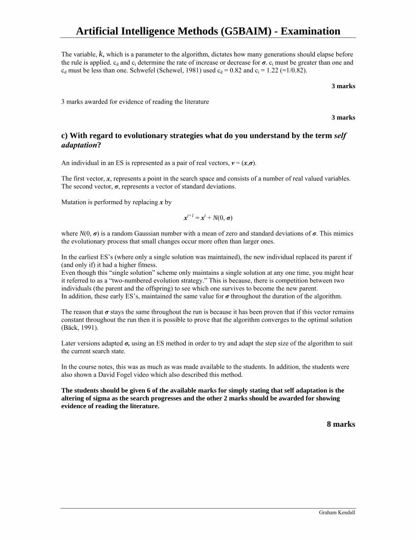
The variable, k, which is a parameter to the algorithm, dictates how many generations should elapse before the rule is applied. cd and ci determine the rate of increase or decrease for σ. ci must be greater than one and cd must be less than one. Schwefel (Schewel, 1981) used cd = 0.82 and ci = 1.22 (=1/0.82).

3 marks 3 marks awarded for evidence of reading the literature

3 marks c) With regard to evolutionary strategies what do you understand by the term self adaptation? An individual in an ES is represented as a pair of real vectors, v = (x,σ). The first vector, x, represents a point in the search space and consists of a number of real valued variables. The second vector, σ, represents a vector of standard deviations. Mutation is performed by replacing x by

xt+1 = xt + N(0, σ) where N(0, σ) is a random Gaussian number with a mean of zero and standard deviations of σ. This mimics the evolutionary process that small changes occur more often than larger ones. In the earliest ES’s (where only a single solution was maintained), the new individual replaced its parent if (and only if) it had a higher fitness. Even though this “single solution” scheme only maintains a single solution at any one time, you might hear it referred to as a “two-numbered evolution strategy.” This is because, there is competition between two individuals (the parent and the offspring) to see which one survives to become the new parent. In addition, these early ES’s, maintained the same value for σ throughout the duration of the algorithm. The reason that σ stays the same throughout the run is because it has been proven that if this vector remains constant throughout the run then it is possible to prove that the algorithm converges to the optimal solution (Bäck, 1991). Later versions adapted σ, using an ES method in order to try and adapt the step size of the algorithm to suit the current search state. In the course notes, this was as much as was made available to the students. In addition, the students were also shown a David Fogel video which also described this method. The students should be given 6 of the available marks for simply stating that self adaptation is the altering of sigma as the search progresses and the other 2 marks should be awarded for showing evidence of reading the literature.

8 marks

Graham Kendall


Graham Kendall

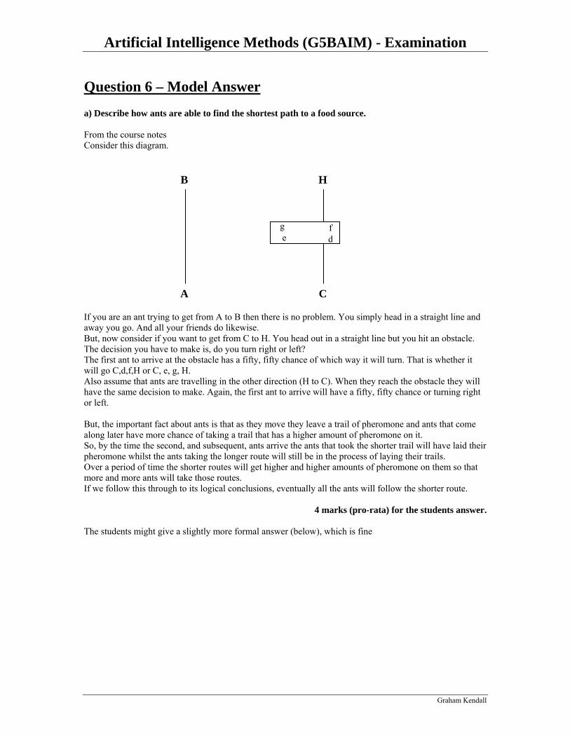
Question 6 – Model Answer a) Describe how ants are able to find the shortest path to a food source. From the course notes Consider this diagram. If you are an ant trying to get from A to B then there is no problem. You simply head in a straight line and away you go. And all your friends do likewise. But, now consider if you want to get from C to H. You head out in a straight line but you hit an obstacle. The decision you have to make is, do you turn right or left? The first ant to arrive at the obstacle has a fifty, fifty chance of which way it will turn. That is whether it will go C,d,f,H or C, e, g, H. Also assume that ants are travelling in the other direction (H to C). When they reach the obstacle they will have the same decision to make. Again, the first ant to arrive will have a fifty, fifty chance or turning right or left. But, the important fact about ants is that as they move they leave a trail of pheromone and ants that come along later have more chance of taking a trail that has a higher amount of pheromone on it. So, by the time the second, and subsequent, ants arrive the ants that took the shorter trail will have laid their pheromone whilst the ants taking the longer route will still be in the process of laying their trails. Over a period of time the shorter routes will get higher and higher amounts of pheromone on them so that more and more ants will take those routes. If we follow this through to its logical conclusions, eventually all the ants will follow the shorter route.

4 marks (pro-rata) for the students answer. The students might give a slightly more formal answer (below), which is fine

A

B

C

H

deg f


Graham Kendall

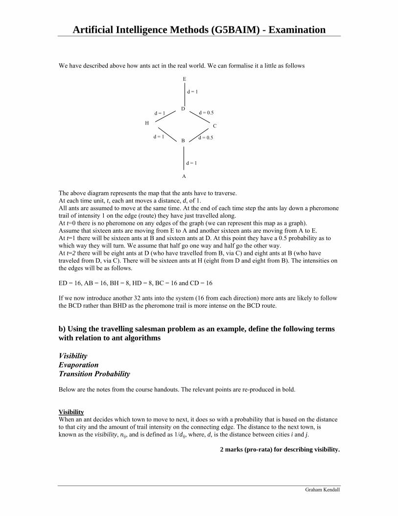
We have described above how ants act in the real world. We can formalise it a little as follows The above diagram represents the map that the ants have to traverse. At each time unit, t, each ant moves a distance, d, of 1. All ants are assumed to move at the same time. At the end of each time step the ants lay down a pheromone trail of intensity 1 on the edge (route) they have just travelled along. At t=0 there is no pheromone on any edges of the graph (we can represent this map as a graph). Assume that sixteen ants are moving from E to A and another sixteen ants are moving from A to E. At t=1 there will be sixteen ants at B and sixteen ants at D. At this point they have a 0.5 probability as to which way they will turn. We assume that half go one way and half go the other way. At t=2 there will be eight ants at D (who have travelled from B, via C) and eight ants at B (who have traveled from D, via C). There will be sixteen ants at H (eight from D and eight from B). The intensities on the edges will be as follows. ED = 16, AB = 16, BH = 8, HD = 8, BC = 16 and CD = 16 If we now introduce another 32 ants into the system (16 from each direction) more ants are likely to follow the BCD rather than BHD as the pheromone trail is more intense on the BCD route. b) Using the travelling salesman problem as an example, define the following terms with relation to ant algorithms Visibility Evaporation Transition Probability Below are the notes from the course handouts. The relevant points are re-produced in bold. Visibility When an ant decides which town to move to next, it does so with a probability that is based on the distance to that city and the amount of trail intensity on the connecting edge. The distance to the next town, is known as the visibility, nij, and is defined as 1/dij, where, d, is the distance between cities i and j.

2 marks (pro-rata) for describing visibility.

A

B

C

D

E

H

d = 1

d = 1

d = 0.5

d = 0.5

d = 1

d = 1


Graham Kendall

Evaporation At each time unit evaporation takes place. This (which also models the real world) is to stop the intensity trails building up unbounded. The amount of evaporation, p, is a value between 0 and 1.

1 mark for describing evaporation. Transition Probability

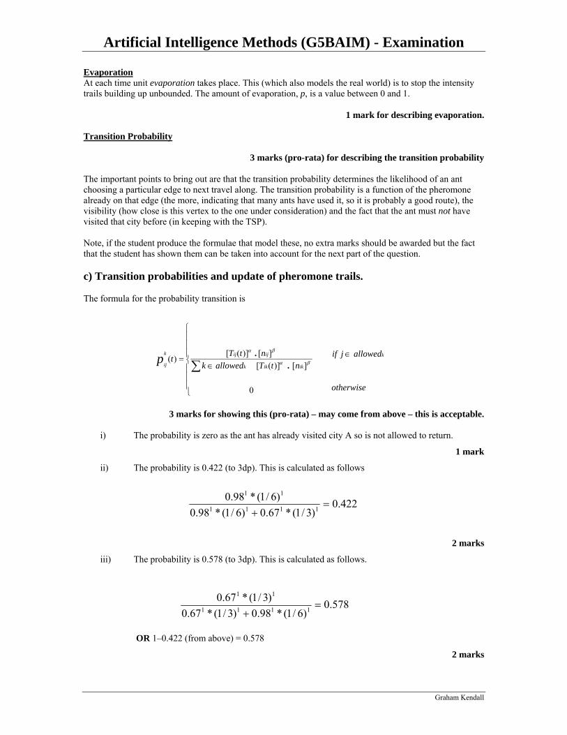
3 marks (pro-rata) for describing the transition probability The important points to bring out are that the transition probability determines the likelihood of an ant choosing a particular edge to next travel along. The transition probability is a function of the pheromone already on that edge (the more, indicating that many ants have used it, so it is probably a good route), the visibility (how close is this vertex to the one under consideration) and the fact that the ant must not have visited that city before (in keeping with the TSP). Note, if the student produce the formulae that model these, no extra marks should be awarded but the fact that the student has shown them can be taken into account for the next part of the question. c) Transition probabilities and update of pheromone trails. The formula for the probability transition is

3 marks for showing this (pro-rata) – may come from above – this is acceptable.

i) The probability is zero as the ant has already visited city A so is not allowed to return.

1 mark

ii) The probability is 0.422 (to 3dp). This is calculated as follows

2 marks

iii) The probability is 0.578 (to 3dp). This is calculated as follows.

OR 1–0.422 (from above) = 0.578

2 marks

otherwise

allowedjifntTallowedk

ntTt k

ikikk

ijijk

ijp ∈

⎪⎪⎪

⎩

⎪⎪⎪

⎨

⎧

∈=∑

0

][)]([][)]([)( .

.βα

βα

422.0)3/1(*67.0)6/1(*98.0

)6/1(*98.01111

11

=+

578.0)6/1(*98.0)3/1(*67.0

)3/1(*67.01111

11

=+


Graham Kendall

iv)

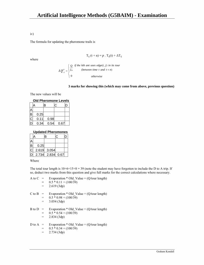
The formula for updating the pheromone trails is

Tij (t + n) = p . Tij(t) + ΔTij where

3 marks for showing this (which may come from above, previous question)

The new values will be

Old Pheromone Levels A B C D A B 0.25 C 0.11 0.98 D 0.34 0.54 0.67 Updated Pheromones A B C D A B 0.25 C 2.619 3.054 D 2.734 2.834 0.67

Where

The total tour length is 10+6+15+8 = 39 (note the student may have forgotten to include the D to A trip. If so, deduct two marks from this question and give full marks for the correct calculations where necessary.

A to C = Evaporation * Old_Value + (Q/tour length) = 0.5 * 0.11 + (100/39) = 2.619 (3dp) C to B = Evaporation * Old_Value + (Q/tour length) = 0.5 * 0.98 + (100/39) = 3.054 (3dp) B to D = Evaporation * Old_Value + (Q/tour length) = 0.5 * 0.54 + (100/39) = 2.834 (3dp) D to A = Evaporation * Old_Value + (Q/tour length) = 0.5 * 0.34 + (100/39) = 2.734 (3dp)

otherwise

ntandttimebetweentouritsinjiedgeusesantkththeif

LQ

kkijT )(

),(

0

+⎪⎩

⎪⎨

⎧

=Δ


Graham Kendall

0.5 mark for getting each correct value (2 marks in total) 0.5 mark for showing each calculation (2 marks in total)

Artificial Intelligence Methods (G5BAIM) - Examination ...pszgxk/aim/2009/exam/2001-02.pdfArtificial...

Documents

Transcript of Artificial Intelligence Methods (G5BAIM) - Examination ...pszgxk/aim/2009/exam/2001-02.pdfArtificial...