ARTIFICIAL INTELLIGENCE - studenthelp62.files.wordpress.com · •Hill climbing •Beam search...
79
ARTIFICIAL INTELLIGENCE LECTURE # 07 Artificial Intelligence 2012 Lecture 07 Delivered By Zahid Iqbal 1
Transcript of ARTIFICIAL INTELLIGENCE - studenthelp62.files.wordpress.com · •Hill climbing •Beam search...
ARTIFICIAL
INTELLIGENCE
LECTURE # 07
Artificial Intelligence 2012 Lecture 07 Delivered By Zahid Iqbal 1

Review of Last Lecture
Artificial Intelligence 2012 Lecture 07 Delivered By Zahid Iqbal 2

Recap
• Review of Last Lecture
• Searching
• State Space Search
• Depth First Search
• Breath First Search
• Iterative Deepening Search
• Bi-Directional Search
Artificial Intelligence 2012 Lecture 07 Delivered By Zahid Iqbal 3

Today’s agenda • Heuristic search
• Hill climbing
• Beam search
• Best first search
• Best first search algorithm
• Greedy approach
• Optimal searches
• Branch and bound
• A* search
• Adversarial search
• Max Min procedure
• Alpha beta pouring
Artificial Intelligence 2012 Lecture 07 Delivered By Zahid Iqbal 4

Informed Search Methods
Heuristic = “to find”, “to discover”
• Blind search: •Search the solution space in an uninformed manner •They simply march through the search space until a solution is found.
•Costly with respect time, space or both •Informed search.
•Search the solution space in informed manner -> HEURISTIC SEARCH •Don’t try to explore all possible search path, rather focus on the path which get you closer to the goal state using some kind of a “ GUIDE”. •A heuristic search makes use of available information in making the
search more efficient.
Artificial Intelligence 2012 Lecture 07 Delivered By Zahid
Iqbal 5

HEURISTIC SEARCH
Heuristics:
Rules for choosing the branches in a state space that are most likely to lead to an acceptable problem solution.
Used when:
• Computational costs are high E.g. Chess
But, Heuristics are fallible. They can lead a search algorithm to a suboptimal solution or fail to find a solution at all.
Artificial Intelligence 2012 Lecture 07 Delivered By Zahid
Iqbal 6

Informed Search Methods
Heuristic = “to find”, “to discover”
•A heuristic is a rule or method that almost always improves the
decision process.
•Generally can’t be sure that you are near the goal, but heuristic is a good guess for the purpose. •E.g. mouse searching for cheese having fresh smell. •Mouse use “fresh smell” as a guide to reach the goal state.
•For example, if in a shop with several checkouts, it is usually best to go
to the one with the shortest queue. This holds true in most cases but
further information could influence this - (1) if you saw that there was a
checkout with only one person in that queue but that the person currently at
the checkout had three trolleys full of shopping and (2) that at the fast-
checkout all the people had only one item, you may choose to go to the fast-
checkout instead. Also, (3) you don't go to a checkout that doesn't have a
cashier - it may have the shortest queue but you'll never get anywhere.
•Heuristic search can be use for
•General purpose ( if you encounter a problem, remember your past weather you solved such type of problem or not, •Specific purpose ( add some form the problem domain) •E.g. car mechanic example, doctor patient example.
Artificial Intelligence 2012 Lecture 07 Delivered By Zahid
Iqbal 7

Heuristic search • Straight line distance of each city form goal city..
S G
C
F D E
A B 5
4
6
3 2
3 3
Artificial Intelligence 2012 Lecture 07 Delivered By Zahid Iqbal 8
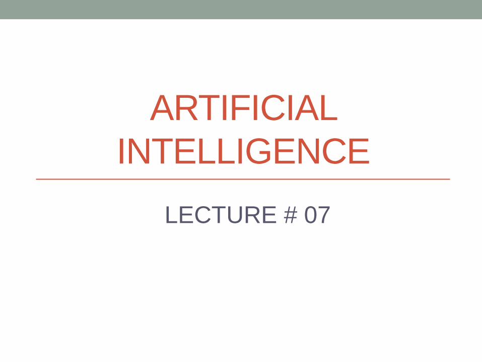
Heuristic search: road map The no show the distance b/w two cities
S G
C
F D E
A B 2
4 4
3 3
2
3 1
3
Artificial Intelligence 2012 Lecture 07 Delivered By Zahid Iqbal 9

Simple heuristic search procedure:
Hill Climbing • Named so because it resembles an eager, but blind
mountain climber, you move in such direction in which
your height increased.
• Your have a altimeter which tells you what will be your
height if you move L, R, U, S.
• Used a heuristic function which measure your height, or
measure remaining distance or find delta.
• And you select such operator which reduce this delta.
• Go uphill along the steepest possible path until you can
go no further.
• As it keeps no history, the algorithm cannot recover from
failures of its strategy
Artificial Intelligence 2012 Lecture 07 Delivered By Zahid Iqbal 10
Hill Climbing
• Simplest way to implement heuristic search
• Expand current state in the search and evaluate its
children
• The best child is selected for further expansion; neither its
siblings nor parents are retained
Artificial Intelligence 2012 Lecture 07 Delivered By Zahid Iqbal 11
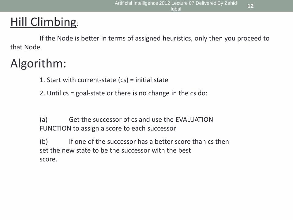
Hill Climbing:
If the Node is better in terms of assigned heuristics, only then you proceed to that Node
Algorithm: 1. Start with current-state (cs) = initial state
2. Until cs = goal-state or there is no change in the cs do:
(a) Get the successor of cs and use the EVALUATION FUNCTION to assign a score to each successor
(b) If one of the successor has a better score than cs then set the new state to be the successor with the best score.
Artificial Intelligence 2012 Lecture 07 Delivered By Zahid
Iqbal 12

IIA1: Hill-climbing (cont)
This simple policy has three well-known drawbacks: 1. Local Maxima: a local maximum as opposed to global maximum. 2. Plateaus: An area of the search space where evaluation function is flat, thus requiring random walk. 3. Ridge: Where there are steep slopes and the search direction is not towards the top but towards the side.
(a)
(b)
(c)
Figure 5.9 Local maxima, Plateaus and
ridge situation for Hill
Climbing
Artificial Intelligence 2012 Lecture 07 Delivered By Zahid Iqbal 13

IIA1: Hill-climbing (cont)
• All these problems can be mapped to situations in our solution space searching. If we are at a state and the heuristics of all the available options take us to a lower value, we might be at local maxima. Similarly, if all the available heuristics take us to no improvement we might be at a plateau. Same is the case with ridge as we can encounter such states in our search tree.
• In each of the previous cases (local maxima, plateaus & ridge), the algorithm reaches a point at which no progress is being made.
• A solution is to do a random-restart hill-climbing - where random initial states are generated, running each until it halts or makes no discernible progress. The best result is then chosen.
Artificial Intelligence 2012 Lecture 07 Delivered By Zahid Iqbal 14
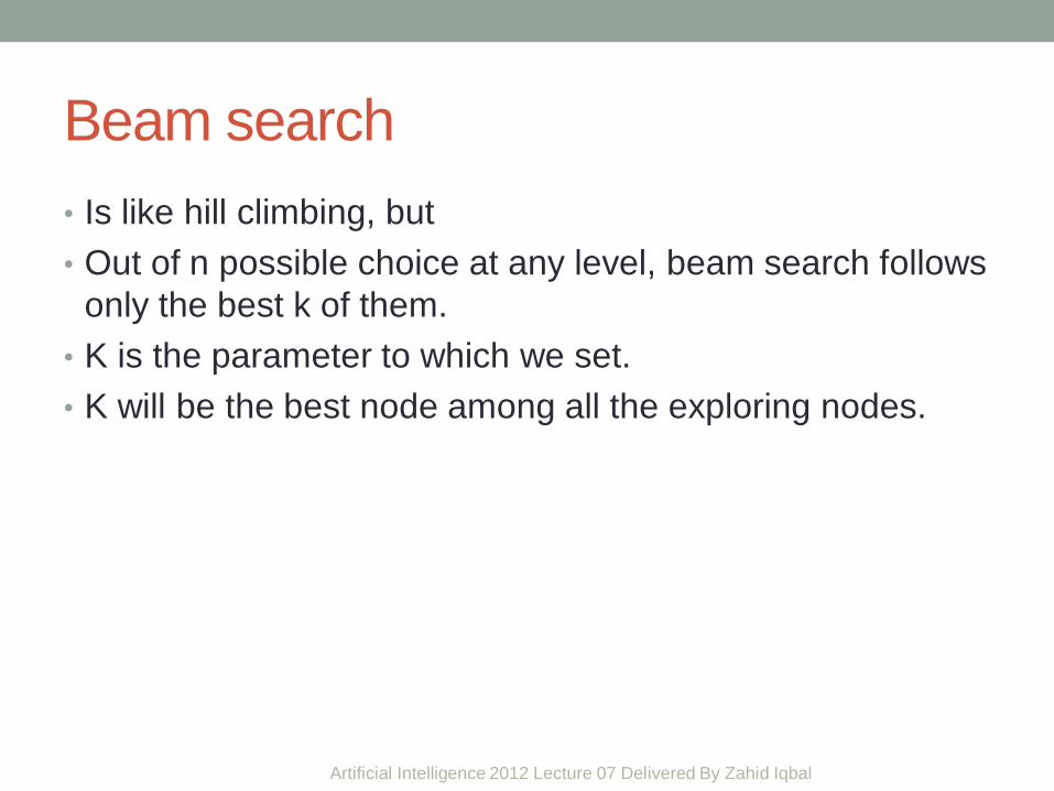
Beam search
• Is like hill climbing, but
• Out of n possible choice at any level, beam search follows
only the best k of them.
• K is the parameter to which we set.
• K will be the best node among all the exploring nodes.
Artificial Intelligence 2012 Lecture 07 Delivered By Zahid Iqbal 15
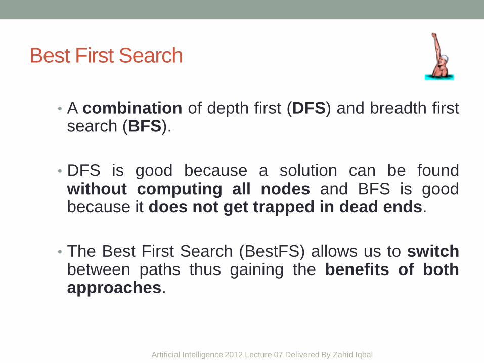
Best First Search
• A combination of depth first (DFS) and breadth first search (BFS).
• DFS is good because a solution can be found without computing all nodes and BFS is good because it does not get trapped in dead ends.
• The Best First Search (BestFS) allows us to switch between paths thus gaining the benefits of both approaches.
Artificial Intelligence 2012 Lecture 07 Delivered By Zahid Iqbal 16

BestFS1: Greedy Search
• This is one of the simplest BestFS strategy.
• Heuristic function: h(n) - prediction of path cost left to the goal.
• Greedy Search: “To minimize the estimated cost to reach the
goal”.
• The node whose state is judged to be closest to the goal state
is always expanded first.
• Two route-finding methods (1) Straight line distance; (2) minimum
Manhattan Distance - movements constrained to horizontal and
vertical directions.
Artificial Intelligence 2012 Lecture 07 Delivered By Zahid Iqbal 17

BestFS1: Greedy Search (cont)
Figure 5.3 Map of Romania with road distances in km, and straight-line distances to Bucharest.
hSLD(n) = straight-line distance between n and the goal location.
Artificial Intelligence 2012 Lecture 07 Delivered By Zahid Iqbal 18
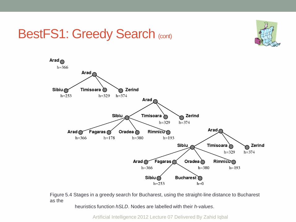
BestFS1: Greedy Search (cont)
Figure 5.4 Stages in a greedy search for Bucharest, using the straight-line distance to Bucharest
as the
heuristics function hSLD. Nodes are labelled with their h-values.
Artificial Intelligence 2012 Lecture 07 Delivered By Zahid Iqbal 19

BestFS1: Greedy Search (cont)
• Noticed that the solution for A S F B is not optimum. It is 32
miles longer than the optimal path A S R P B.
• The strategy prefers to take the biggest bite possible out of the
remaining cost to reach the goal, without worrying whether this is
the best in the long run - hence the name ‘greedy search’.
• Greed is one of the 7 deadly sins, but it turns out that GS perform
quite well though not always optimal.
• GS is susceptible to false start. Consider the case of going from
Iasi to Fagaras. Neamt will be consider before Vaului even though
it is a dead end.
Artificial Intelligence 2012 Lecture 07 Delivered By Zahid Iqbal 20

BestFS1: Greedy Search (cont)
• GS resembles DFS in the way it prefers to follow a single path all
the way to the goal, but will back up when it hits a dead end.
• Thus suffering the same defects as DFS - not optimal and is
incomplete.
• The worst-case time complexity for GS is O(bm), where m is the
max depth of the search space.
• With good heuristic function, the space and time complexity
can be reduced substantially.
Artificial Intelligence 2012 Lecture 07 Delivered By Zahid Iqbal 21
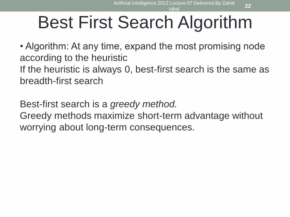
• Algorithm: At any time, expand the most promising node
according to the heuristic
If the heuristic is always 0, best-first search is the same as
breadth-first search
Best-first search is a greedy method.
Greedy methods maximize short-term advantage without
worrying about long-term consequences.
Best First Search Algorithm
Artificial Intelligence 2012 Lecture 07 Delivered By Zahid
Iqbal 22

Best First Search Method Function best_First_Search; Begin open := [Start]; closed:=[]; while open != [] do begin
remove the leftmost state from open, call it X; If X = goal then return the path from Start to X
Else begin Generate children of X;
For each child of X do If the child is not on open or closed then begin assign the child a heuristic value; add the child to open end; End;
Put X on closed; Re-order states on open by heuristic merit (best leftmost)
End; Return FAIL End.
Artificial Intelligence 2012 Lecture 07 Delivered By Zahid
Iqbal 23
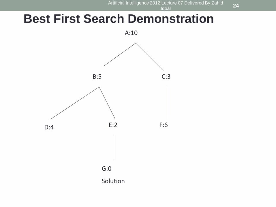
F:6
B:5
D:4 E:2
G:0
Solution
C:3
A:10
Best First Search Demonstration
Artificial Intelligence 2012 Lecture 07 Delivered By Zahid
Iqbal 24

1. Open [A:10] : closed []
2. Evaluate A:10; open [C:3,B:5]; closed [A:10]
3. Evaluate C:3; open [B:5,F:6]; closed [C:3,A:10]
4. Evaluate B:5; open [E:2,D:4,F:6]; closed [C:3,B:5,A:10].
5. Evaluate E:2; open [G:0,D:4,F:6];
closed [E:2,C:3,B:5,A:10]
6. Evaluate G:0; the solution / goal is reached
Best First Search Demonstration
Artificial Intelligence 2012 Lecture 07 Delivered By Zahid
Iqbal 25

Best First Search Demonstration
Artificial Intelligence 2012 Lecture 07 Delivered By Zahid
Iqbal 26
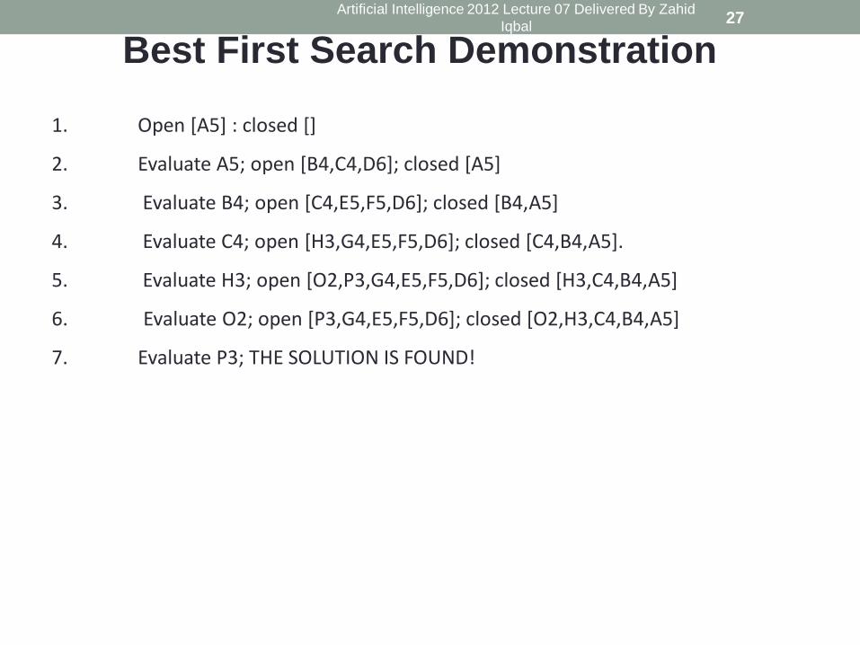
1. Open [A5] : closed []
2. Evaluate A5; open [B4,C4,D6]; closed [A5]
3. Evaluate B4; open [C4,E5,F5,D6]; closed [B4,A5]
4. Evaluate C4; open [H3,G4,E5,F5,D6]; closed [C4,B4,A5].
5. Evaluate H3; open [O2,P3,G4,E5,F5,D6]; closed [H3,C4,B4,A5]
6. Evaluate O2; open [P3,G4,E5,F5,D6]; closed [O2,H3,C4,B4,A5]
7. Evaluate P3; THE SOLUTION IS FOUND!
Best First Search Demonstration
Artificial Intelligence 2012 Lecture 07 Delivered By Zahid
Iqbal 27

•If the evaluation function is good best first search may
significantly cut the amount of search requested
otherwise.
•If the evaluation function is heavy / very expensive the
benefits may be overweighed by the cost of assigning a
score
Restrictions on Evaluation Function
Artificial Intelligence 2012 Lecture 07 Delivered By Zahid
Iqbal 28
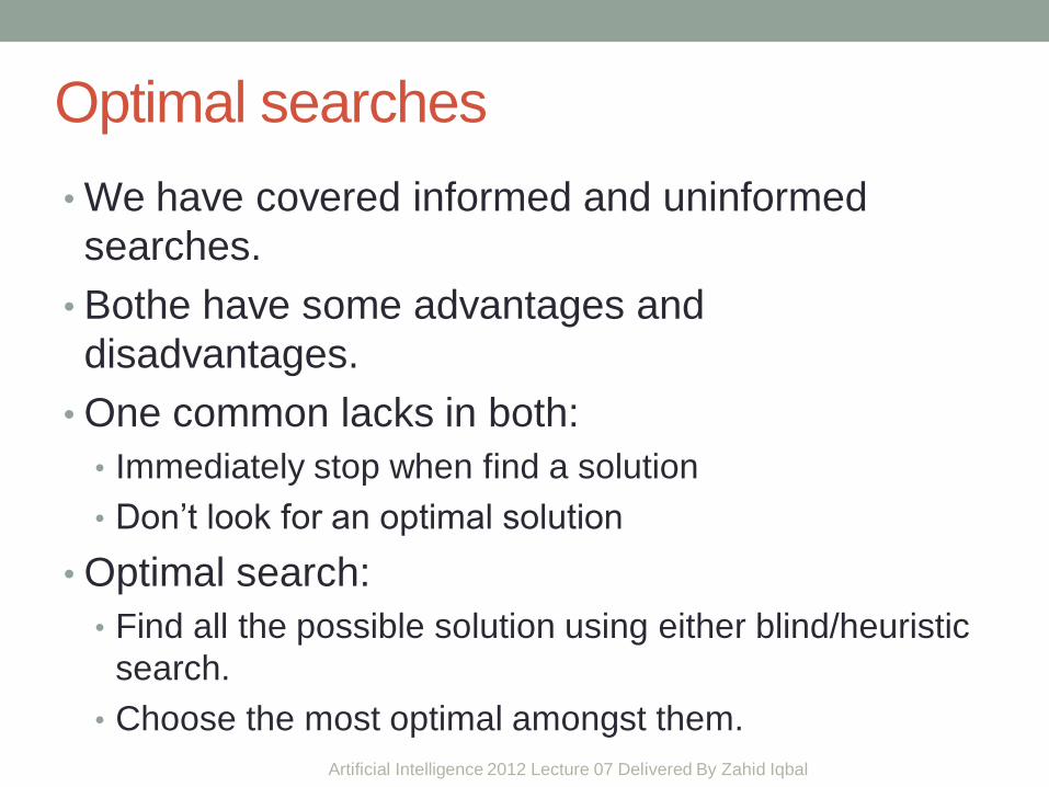
Optimal searches
• We have covered informed and uninformed
searches.
• Bothe have some advantages and
disadvantages.
• One common lacks in both:
• Immediately stop when find a solution
• Don’t look for an optimal solution
• Optimal search:
• Find all the possible solution using either blind/heuristic
search.
• Choose the most optimal amongst them.
Artificial Intelligence 2012 Lecture 07 Delivered By Zahid Iqbal 29

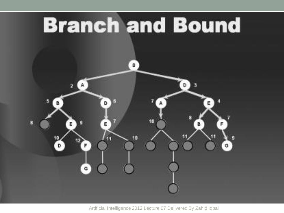
Branch and bound • Some how related to heuristic search.
• Cut of the unnecessary search.
S
G B F
D
E A
9 9
Artificial Intelligence 2012 Lecture 07 Delivered By Zahid Iqbal 30

.
• .
Branch and bound The no show the distance b/w two cities
S G
C
F E
A B 2
4 4
3 3
2
3 1
3
D
Artificial Intelligence 2012 Lecture 07 Delivered By Zahid Iqbal 31

Artificial Intelligence 2012 Lecture 07 Delivered By Zahid Iqbal 32
Artificial Intelligence 2012 Lecture 07 Delivered By Zahid Iqbal 33

A* • A* (pronounced "A star") is a best-first, graph search algorithm that finds the least-cost path from a given initial node to one goal node (out of one or more possible goals).
• Improve version of branch and bound.
• Uses a distance-plus-cost heuristic function (usually denoted f(x)) to determine the order in which the search visits nodes in the tree.
• Initially called algorithm A. Since using this algorithm yields optimal behavior for a given heuristic, it has been called A*.
Artificial Intelligence 2012 Lecture 07 Delivered By Zahid Iqbal 34

Distance-Plus-Cost Heuristics function
• The distance-plus-cost heuristic is a sum of two functions:
• The path-cost function (usually denoted g(x)): cost from the starting
node to the current node.
• A heuristic estimate of the distance to the goal (usually denoted
h(x)).
• Total Cost: f(x) = g(x) + h(x)
Artificial Intelligence 2012 Lecture 07 Delivered By Zahid Iqbal 35

.
• .
A* Search Algorithm The no show the distance b/w two cities
And the color no shows the under estimated
distance between that particular node and the goal
node.
S G
C
F E
A B 2
4 4
3 3
2
3 1
3
D
8
2 3
5
0
2 5
6 Artificial Intelligence 2012 Lecture 07 Delivered By Zahid Iqbal 36

Artificial Intelligence 2012 Lecture 07 Delivered By Zahid Iqbal 37

Artificial Intelligence 2012 Lecture 07 Delivered By Zahid Iqbal 38

A* Search Algorithm
• At every step, take node n from the front of the queue
• Enqueue all its successors n" with priorities:
• f(n") = g(n") + h(n")
= cost of getting to n" + estimated cost from n" to goal
• Terminate when a goal state is popped from the queue.
Artificial Intelligence 2012 Lecture 07 Delivered By Zahid Iqbal 39

A* Search Method Function A*; Begin open := [Start]; closed:=[]; while open != [] do begin
remove the leftmost state from open, call it X; If X = goal then return the path from Start to X
Else begin Generate children of X;
For each child (m) of X do case the child (m) is not on open or closed then begin assign the child (m) a heuristic value; { g(m) = g(n) + C(n,m) f(m) = g(m) + h(m) } add the child to open end;
Artificial Intelligence 2012 Lecture 07 Delivered By Zahid
Iqbal 40

the child (m) belongs to open or closed then begin g(m) = min{g(m), g(n) + C(n,m)} f(m) = g(m) + h(m) End; if f(m) has decreased and m belongs to closed then move m to open End
Put X on closed; Re-order states on open by heuristic merit (best leftmost)
End; Return FAIL End.
Artificial Intelligence 2012 Lecture 07 Delivered By Zahid
Iqbal 41

Examples of Heuristics Artificial Intelligence 2012 Lecture 07 Delivered By Zahid
Iqbal 42

Last Solution
Artificial Intelligence 2012 Lecture 07 Delivered By Zahid
Iqbal 43
Adversarial Search
Adversary:= opponent
We have experience in search where we assume that we are the only
intelligent being and we have explicit control over the “world”.
Your are the only agent in complete search space so you are
responsible what you have done in achieving your goal
Adversarial Search
Lets consider what happens when we relax those assumptions. Problem solving agent is not alone any more
Multiagent, conflict You have no more control over the search space, what to done next. You will be given just one chance to apply a legal operator to move. Two searches will be in progress at the same time, each try to beat the other search.
Artificial Intelligence 2012 Lecture 07 Delivered By Zahid
Iqbal 44
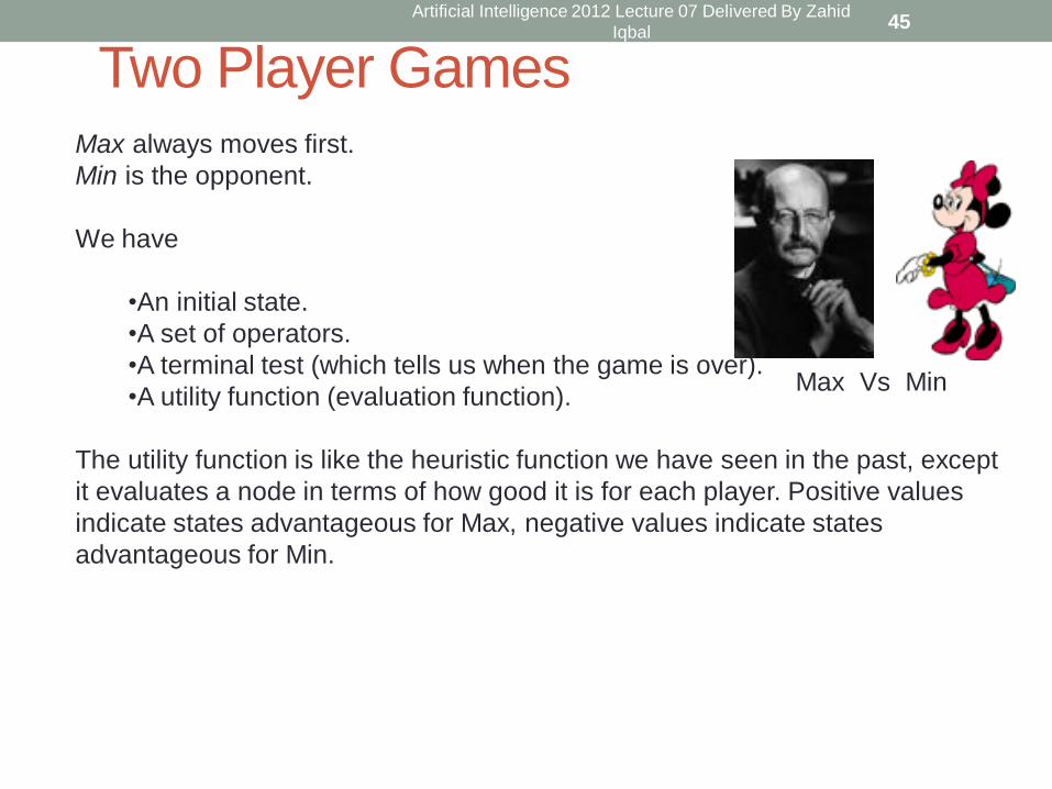
Two Player Games Max always moves first.
Min is the opponent.
We have
•An initial state.
•A set of operators.
•A terminal test (which tells us when the game is over).
•A utility function (evaluation function).
The utility function is like the heuristic function we have seen in the past, except
it evaluates a node in terms of how good it is for each player. Positive values
indicate states advantageous for Max, negative values indicate states
advantageous for Min.
Max Vs Min
Artificial Intelligence 2012 Lecture 07 Delivered By Zahid
Iqbal 45

X O
X
X O
X
X
O
X X O
O O X
X
X O X
O
O O
X X X
O
O
X
... ... ...
-1 O 1
Utility
Terminal
States
Max
Min
Max ... ... ... ... ... ...
Artificial Intelligence 2012 Lecture 07 Delivered By Zahid
Iqbal 46

Search with an opponent
• Trivial approximation: generating the tree for all moves
• Terminal moves are tagged with a utility value, for example: “+1” or “-1” depending on if the winner is MAX or MIN.
• The goal is to find a path to a winning state.
• Even if a depth-first search would minimize memory space, in complex games this kind of search cannot be carried out.
• Even a simple game like tic-tac-toe is too complex to draw the entire game tree.
Artificial Intelligence 2012 Lecture 07 Delivered By Zahid Iqbal 47
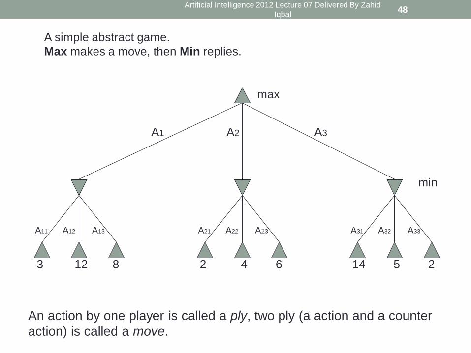
3 12 8
A11 A12 A13
2 4 6
A21 A22 A23
14 5 2
A31 A32 A33
max
A simple abstract game.
Max makes a move, then Min replies.
A3 A2 A1
An action by one player is called a ply, two ply (a action and a counter
action) is called a move.
min
Artificial Intelligence 2012 Lecture 07 Delivered By Zahid
Iqbal 48

• Generate the game tree down to the terminal nodes.
• Apply the utility function to the terminal nodes to gets its value.
• For a S set of sibling nodes, pass up to the parent…
• the lowest value in S if the siblings are (moves by max)
• the largest value in S if the siblings are moves by min)
• Recursively do the above, until the backed-up values reach the
initial state.
• The value of the initial state is the minimum score for Max.
The Minimax Algorithm
Artificial Intelligence 2012 Lecture 07 Delivered By Zahid
Iqbal 49

The minimax algorithm
Artificial Intelligence 2012 Lecture 07 Delivered By Zahid Iqbal 50
3 12 8
A11 A12 A13
3
2 4 6
A21 A22 A23
2
14 5 2
A31 A32 A33
2
3
A3 A2 A1
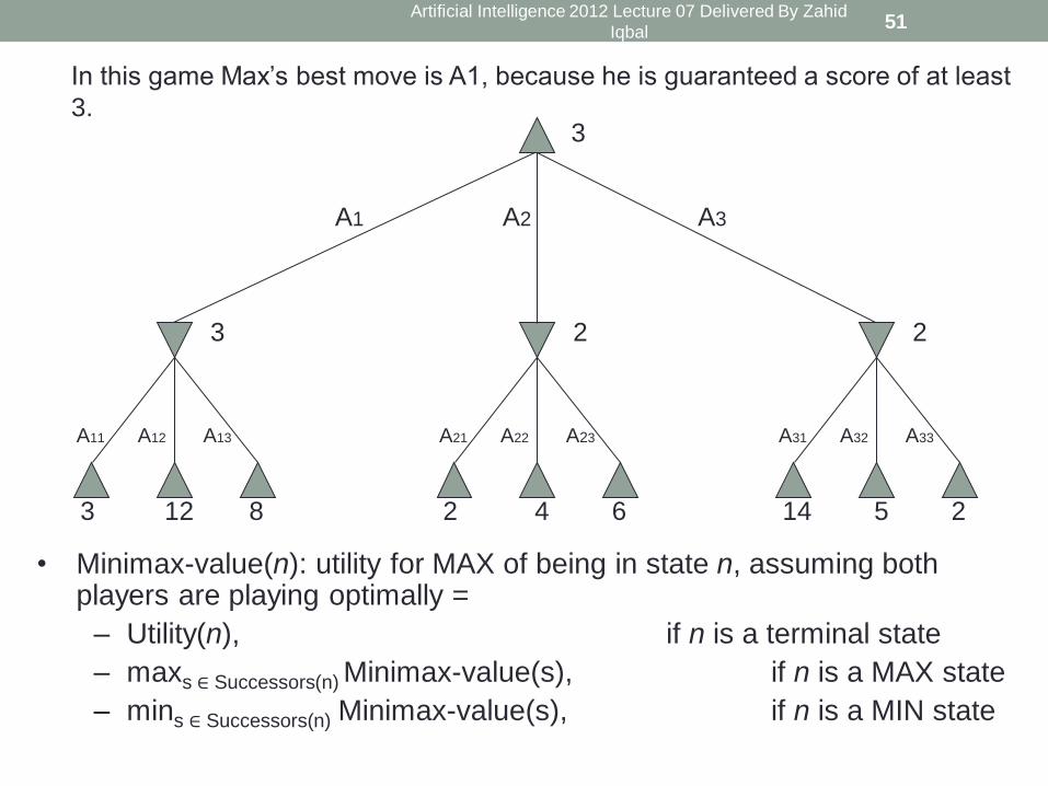
In this game Max’s best move is A1, because he is guaranteed a score of at least
3.
• Minimax-value(n): utility for MAX of being in state n, assuming both players are playing optimally =
– Utility(n), if n is a terminal state
– maxs ∈ Successors(n) Minimax-value(s), if n is a MAX state
– mins ∈ Successors(n) Minimax-value(s), if n is a MIN state
Artificial Intelligence 2012 Lecture 07 Delivered By Zahid
Iqbal 51

The minimax algorithm
• The algorithm first recurses down to the tree bottom-left
nodes
• and uses the Utility function on them to discover that their
values are 3, 12 and 8. 52
Artificial Intelligence 2012 Lecture 07 Delivered By Zahid Iqbal 52
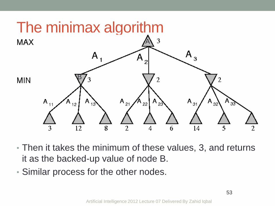
The minimax algorithm
• Then it takes the minimum of these values, 3, and returns
it as the backed-up value of node B.
• Similar process for the other nodes.
53
B
A
Artificial Intelligence 2012 Lecture 07 Delivered By Zahid Iqbal 53

Although the Minimax algorithm is optimal, there is a
problem…
The time complexity is O(bm) where b is the effective branching factor (legal moves at
each point) and m is the depth of the terminal states (maximum depth of the tree).
(Note space complexity is only linear in b and m, because we can do depth first
search).
One possible solution is to do depth limited Minimax search.
• Search the game tree as deep as you can in the given time.
• Evaluate the fringe (border) nodes with the utility function.
• Back up the values to the root.
• Choose best move, repeat.
We would like
to do Minimax
on this full
game tree...
… but we don’t
have time, so
we will explore
it to some
manageable
depth.
cutoff
Artificial Intelligence 2012 Lecture 07 Delivered By Zahid
Iqbal 54

The minimax algorithm: problems
• For real games the time cost of minimax is totally
impractical, but this algorithm serves as the basis:
• for the mathematical analysis of games and
• for more practical algorithms
• Problem with minimax search:
• The number of game states it has to examine is exponential in
the number of moves.
• Unfortunately, the exponent can’t be eliminated, but it can
be cut in half.
55
Artificial Intelligence 2012 Lecture 07 Delivered By Zahid Iqbal 55
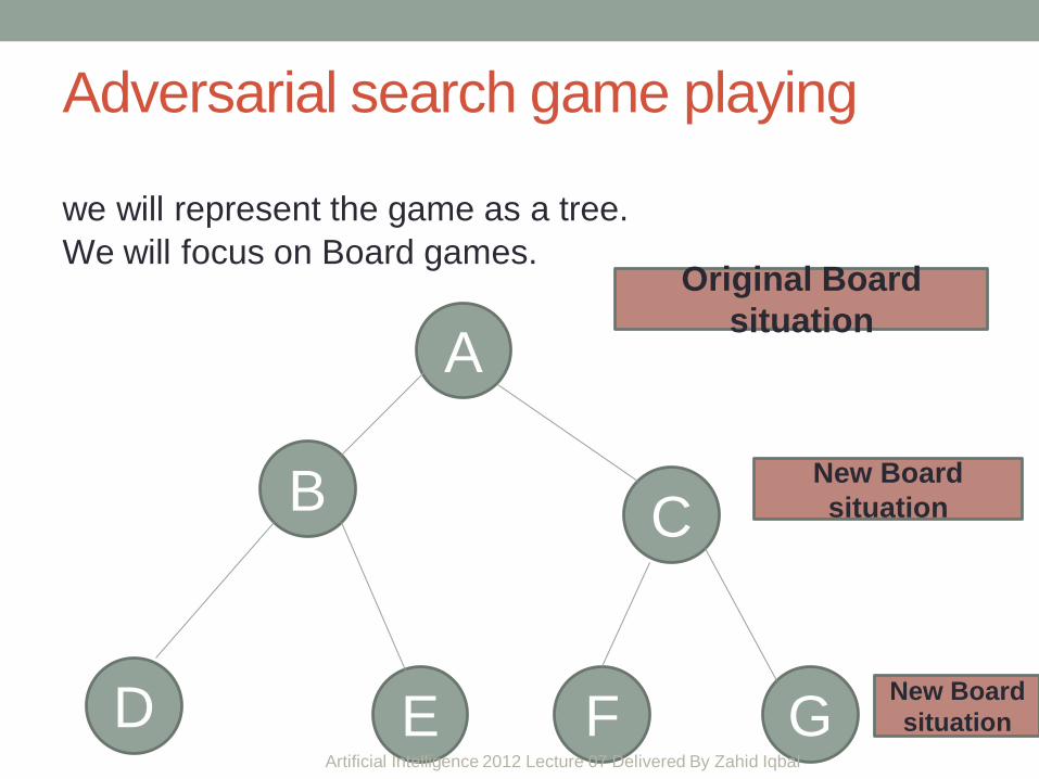
Adversarial search game playing
we will represent the game as a tree.
We will focus on Board games.
G
C
F E
A
B
D
Original Board
situation
New Board
situation
New Board
situation
Artificial Intelligence 2012 Lecture 07 Delivered By Zahid Iqbal 56
Alpha-beta pruning
• It is possible to compute the correct minimax decision
without looking at every node in the game tree.
• Alpha-beta pruning allows to eliminate large parts of the
tree from consideration, without influencing the final
decision.
57
Artificial Intelligence 2012 Lecture 07 Delivered By Zahid Iqbal 57

Alpha-Beta Pruning
3 12 8
A11 A12 A13
3
2
A21 A22 A23
2
14 5 2
A31 A32 A33
2
3
A3 A2 A1
If you have an idea that is surely bad, don't take the
time to see how truly awful it is.
Artificial Intelligence 2012 Lecture 07 Delivered By Zahid
Iqbal 58
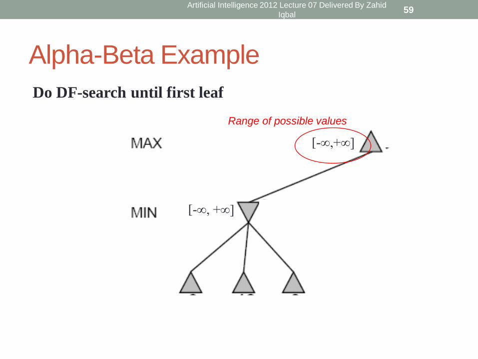
Alpha-Beta Example
[-∞, +∞]
[-∞,+∞]
Range of possible values
Do DF-search until first leaf
Artificial Intelligence 2012 Lecture 07 Delivered By Zahid
Iqbal 59

Alpha-Beta Example (continued)
[-∞,3]
[-∞,+∞]
Artificial Intelligence 2012 Lecture 07 Delivered By Zahid
Iqbal 60

Alpha-Beta Example (continued)
[-∞,3]
[-∞,+∞]
Artificial Intelligence 2012 Lecture 07 Delivered By Zahid
Iqbal 61
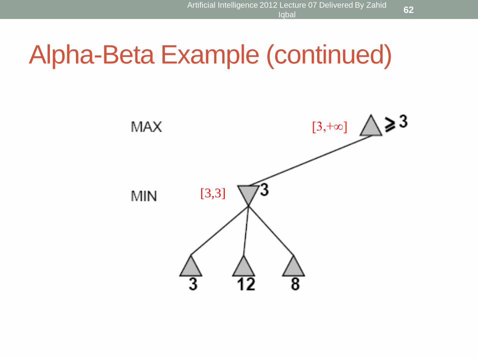
Alpha-Beta Example (continued)
[3,+∞]
[3,3]
Artificial Intelligence 2012 Lecture 07 Delivered By Zahid
Iqbal 62

Alpha-Beta Example (continued)
[-∞,2]
[3,+∞]
[3,3]
This node is worse
for MAX
Artificial Intelligence 2012 Lecture 07 Delivered By Zahid
Iqbal 63
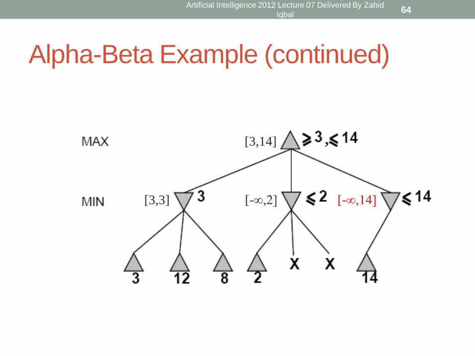
Alpha-Beta Example (continued)
[-∞,2]
[3,14]
[3,3] [-∞,14]
,
Artificial Intelligence 2012 Lecture 07 Delivered By Zahid
Iqbal 64

Alpha-Beta Example (continued)
[−∞,2]
[3,5]
[3,3] [-∞,5]
,
Artificial Intelligence 2012 Lecture 07 Delivered By Zahid
Iqbal 65
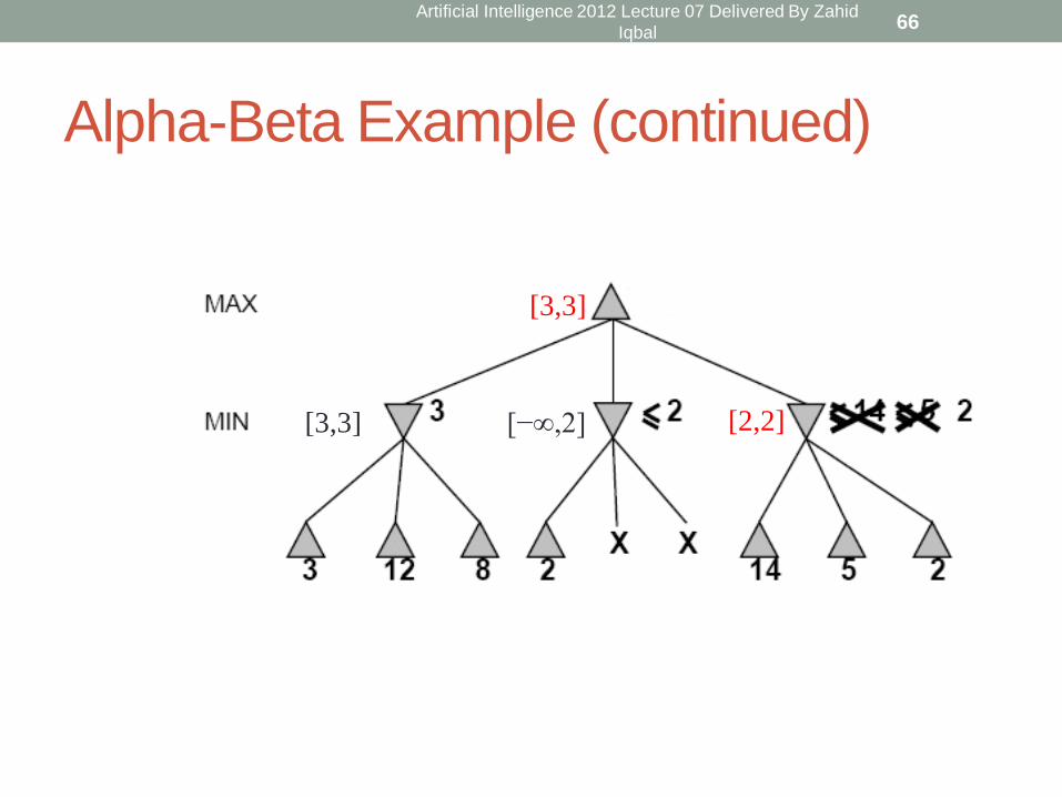
Alpha-Beta Example (continued)
[2,2] [−∞,2]
[3,3]
[3,3]
Artificial Intelligence 2012 Lecture 07 Delivered By Zahid
Iqbal 66

Alpha-Beta Example (continued)
[2,2] [-∞,2]
[3,3]
[3,3]
Artificial Intelligence 2012 Lecture 07 Delivered By Zahid
Iqbal 67
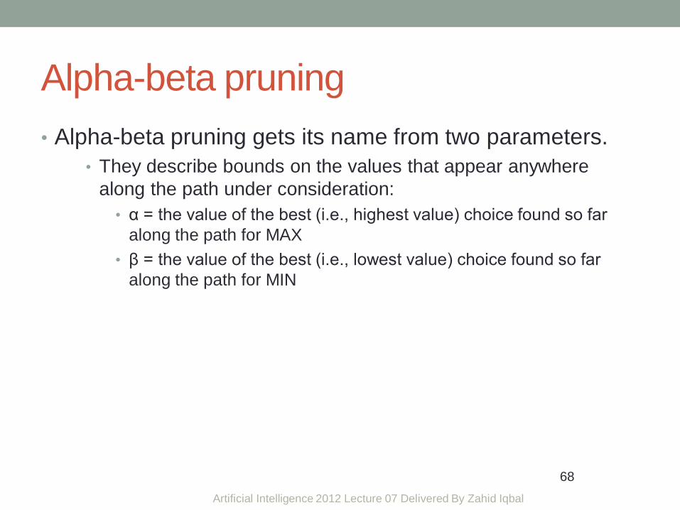
Alpha-beta pruning
• Alpha-beta pruning gets its name from two parameters.
• They describe bounds on the values that appear anywhere
along the path under consideration:
• α = the value of the best (i.e., highest value) choice found so far
along the path for MAX
• β = the value of the best (i.e., lowest value) choice found so far
along the path for MIN
68
Artificial Intelligence 2012 Lecture 07 Delivered By Zahid Iqbal 68

Alpha-beta pruning
• Alpha-beta search updates the values of α and β as it
goes along.
• It prunes the remaining branches at a node (i.e.,
terminates the recursive call)
• as soon as the value of the current node is known to be worse
than the current α or β value for MAX or MIN, respectively.
69
Artificial Intelligence 2012 Lecture 07 Delivered By Zahid Iqbal 69

The alpha-beta search algorithm
Artificial Intelligence 2012 Lecture 07 Delivered By Zahid Iqbal 70

Alpha-Beta Example
Do DF-search until first leaf
Artificial Intelligence 2012 Lecture 07 Delivered By Zahid
Iqbal 71
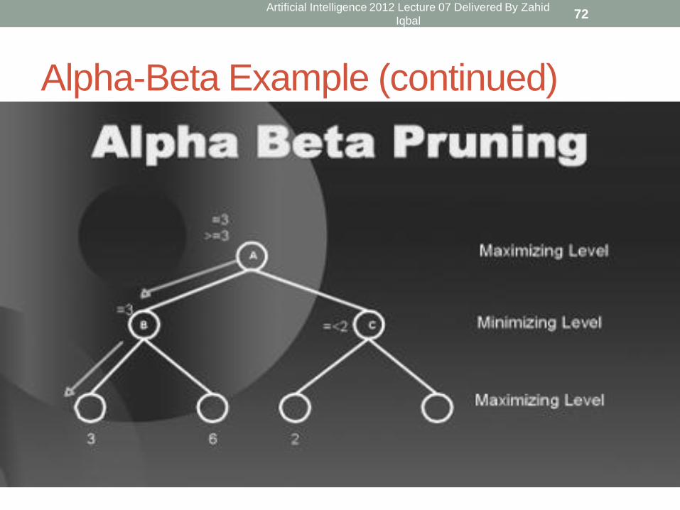
Alpha-Beta Example (continued)
Artificial Intelligence 2012 Lecture 07 Delivered By Zahid
Iqbal 72
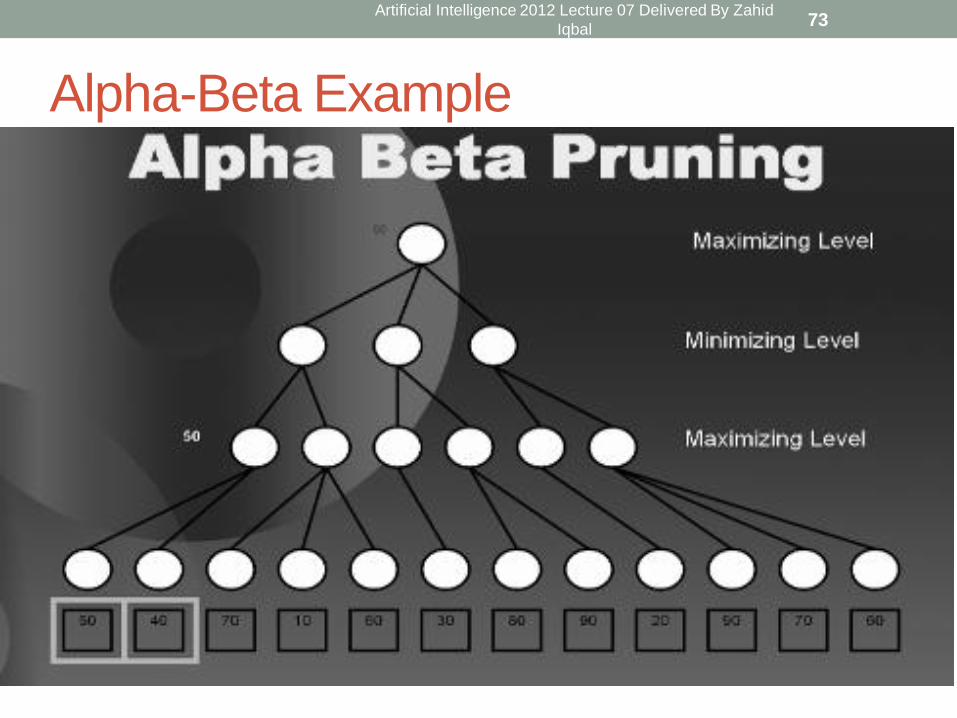
Alpha-Beta Example
Artificial Intelligence 2012 Lecture 07 Delivered By Zahid
Iqbal 73
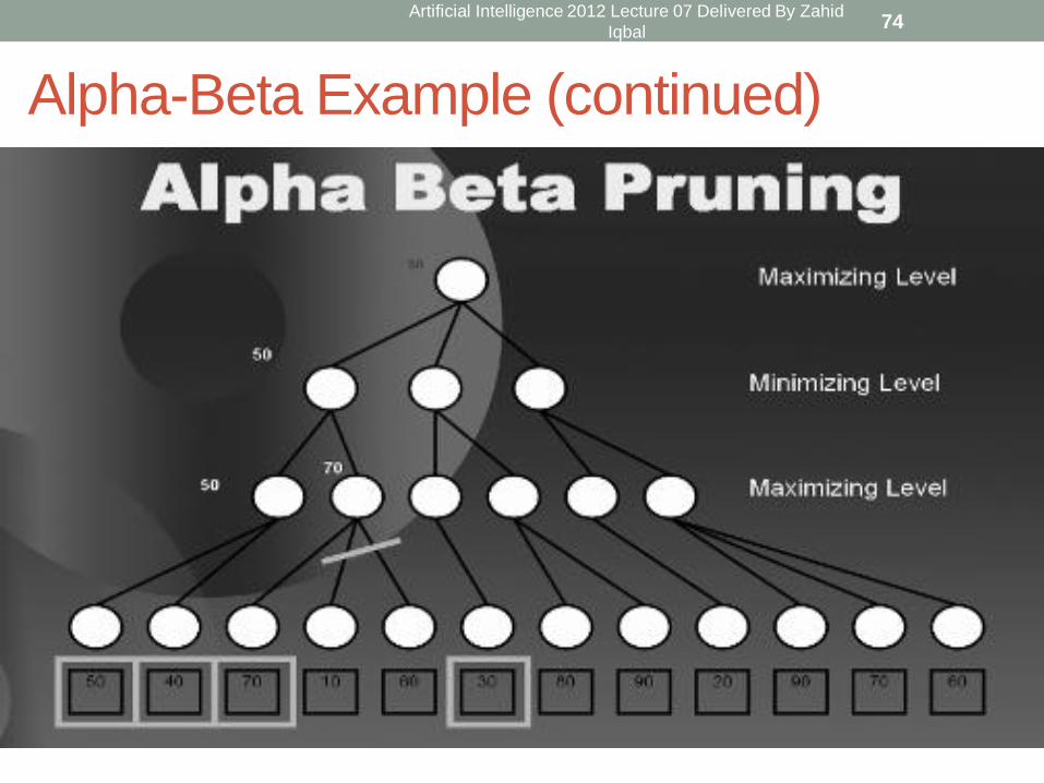
Alpha-Beta Example (continued)
Artificial Intelligence 2012 Lecture 07 Delivered By Zahid
Iqbal 74

Alpha-Beta Example (continued)
Artificial Intelligence 2012 Lecture 07 Delivered By Zahid
Iqbal 75

Alpha-Beta Example (continued)
Artificial Intelligence 2012 Lecture 07 Delivered By Zahid
Iqbal 76
Final comments about alpha-beta pruning
• Pruning does not affect final results.
• Entire subtrees can be pruned, not just leaves.
• Good move ordering improves effectiveness of
pruning.
• With perfect ordering, time complexity is
O(bm/2).
• Effective branching factor of sqrt(b)
• Consequence: alpha-beta pruning can look twice as
deep as minimax in the same amount of time.
77
Artificial Intelligence 2012 Lecture 07 Delivered By Zahid Iqbal 77
References
• Artificial Intelligence, A modern approach by Russell:
(Chapter 4 & 6)
• Artificial Intelligence: Structures and Strategies for
Complex Problem Solving by George F Luger:
(Chapter 4)
Artificial Intelligence 2012 Lecture 07 Delivered By Zahid Iqbal 78

End of Lecture
Artificial Intelligence 2012 Lecture 07 Delivered By Zahid Iqbal 79