Artificial Immune System Approach for Air Combat Maneuvering

John Kaneshige*, Kalmanje Krishnakumar

NASA Ames Research Center, Moffett Field, CA, USA 94035

ABSTRACT

Since future air combat missions will involve both manned and unmanned aircraft, the primary motivation for this

research is to enable unmanned aircraft with intelligent maneuvering capabilities. During air combat maneuvering, pilots

use their knowledge and experience of maneuvering strategies and tactics to determine the best course of action. As a

result, we try to capture these aspects using an artificial immune system approach. The biological immune system

protects the body against intruders by recognizing and destroying harmful cells or molecules. It can be thought of as a

robust adaptive system that is capable of dealing with an enormous variety of disturbances and uncertainties. However,

another critical aspect of the immune system is that it can remember how previous encounters were successfully

defeated. As a result, it can respond faster to similar encounters in the future. This paper describes how an artificial

immune system is used to select and construct air combat maneuvers. These maneuvers are composed of autopilot mode

and target commands, which represent the low-level building blocks of the parameterized system. The resulting

command sequences are sent to a tactical autopilot system, which has been enhanced with additional modes and an

aggressiveness factor for enabling high performance maneuvers. Just as vaccinations train the biological immune system

how to combat intruders, training sets are used to teach the maneuvering system how to respond to different enemy

aircraft situations. Simulation results are presented, which demonstrate the potential of using immunized maneuver

selection for the purposes of air combat maneuvering.

Keywords: Evolutionary, genetic, artificial, immune, tactical, maneuvering, unmanned, aircraft, UAV, ACM

1. INTRODUCTION

Unmanned Aerial Vehicles (UAVs) have been demonstrated as effective platforms for performing missions requiring

long endurance flight and operating in areas that may be too dangerous for humans. As their role expands, from remotely

controlled to semi-autonomous and autonomous operations, challenges are presented which require the development and

application of intelligent systems [1]. These systems must be capable of making reliable decisions under varying

conditions. As a result, they must incorporate aspects of the experience, reasoning and learning abilities of a pilot.

A high level of autonomy is desired for future unmanned combat systems because lethality and survivability can be

improved with much less communications bandwidth than would be necessary for preprogrammed or remotely operated

systems [2]. However, there are a number of technical challenges that must be addressed prior to implementation. These

challenges include situational awareness, three-dimensional mapping, sensor and data fusion, natural language

processing, adaptation and learning, image understanding, and human-machine cooperation [3]. The purpose of this

research is to investigate the application of an artificial immune system to address some of the adaptation and learning

challenges that pertain to autonomous Air Combat Maneuvering (ACM).

ACM has been described as the art of maneuvering a combat aircraft in order to obtain a position from which an attack

can be made on another aircraft [4]. It relies on offensive and defensive Basic Flight Maneuvers (BFMs) in order to gain

an advantage over an aerial opponent. BFMs represent the primary maneuvers that can be viewed as the building blocks

for ACM. They are composed of accelerations/decelerations, climbs/descents, and turns that can be performed in

combination relative to other aircraft. Pilots use their training and experience of combat tactics, along with their

knowledge of aircraft capabilities, to determine which BFMs to perform and how to manipulate them [5].

A biological immune system performs a similar role as it protects the body against infectious agents. In this case,

intruder aircraft represent the antigens (or problems) characterized by their relative positions and velocities. Maneuvers

represent the antibodies (or solutions) composed of commonly used BFMs. An artificial immune system is used to

* john.t.kaneshige@nasa.gov; phone 1 650 604-0710; fax 1 650 604-3594; nasa.gov

construct the maneuvers that are necessary for responding to different air combat situations. This is accomplished by

emulating the adaptive capabilities of the biological immune system using a combination of genetic and evolutionary

algorithms. Another critical aspect of the biological immune system is that it possesses strong memory retention

characteristics. It can remember how previous encounters were successfully defeated so it can respond faster to similar

situations in the future. This is especially critical for ACM, where split-second decisions can mean the difference

between successful and unsuccessful encounters. The artificial immune system emulates this ability by establishing a

database of successful solutions, and categorizing them according to their problem-to-solution mapping characteristics.

This mapping can be further strengthened over time. The equivalent of vaccinations can be provided through the use of

training sets to introduce the artificial immune system to a variety of problems. This represents the equivalent of the

training pilots receive in order to gain the experience necessary for making quick decisions under combat situations.

This paper contains an overview of the immunized maneuver selection methodology, a detailed description of the

implementation, and some test results from simulations evaluating one-verses-one maneuvering of similar aircraft. Since

this research was primarily focused on the adaptation and learning challenges of autonomous ACM, it was assumed that

relative positions and velocities of intruders were known. Furthermore, it was also assumed that human operators, or

other intelligent systems, would be responsible for making strategic oriented decisions such as selecting attack

formations, determining pre-attack positioning and engagement/disengagement criteria.

2. METHODOLOGY

Immunology is the science of built-in defense mechanisms that are present in all living beings to protect against external

attacks. A biological immune system can be thought of as a robust, adaptive system capable of dealing with an enormous

variety of disturbances and uncertainties. During the generation of the immune response, the system receives continuous

feedback from the antigen-antibody complex resulting in a generation of an increasingly specific antibody response.

This represents a learning paradigm that develops solutions that continually increase in accuracy. The artificial immune

system models the search for a solution after the generation of an immune response wherein the optimal solution is

achieved by rapid mutation and recombination of a genetic representation of the solution space. In this case, genes are

represented by a finite number of discrete building blocks that can be thought of as pieces of a puzzle, which must be put

together in a specific way to neutralize, remove, or destroy each unique disturbance the system encounters. For ACM,

these building blocks consist of BFMs that must be combined and manipulated during immunized maneuver selection.

2.1 Biological Immune System

The adaptive response of the biological immune system is driven by the presence of a threat. Cells that most effectively

nullify that threat receive the strongest signals to replicate. The basic components of the immune system are white blood

cells, or lymphocytes, which are produced in the bone marrow. Some lymphocytes only live for a few days, so the bone

marrow is constantly making new cells to replace the old ones in the blood. There are two major classes of lymphocytes:

B-cells, which mature in the bone barrow; and T-cells, which travel through the bloodstream to the thymus where they

become fully developed as either Helper T-cells or Killer T-cells.

Once B-cells are released into the bloodstream they perform the roll of immune surveillance. Immune recognition is

based on the complementarity between the binding region of B-cell receptors and a portion of the antigen called an

epitope. B-cell receptors are essentially non-soluble antibodies that are attached to the B-cells. While all the receptors on

a particular B-cell are the same, the unique genetic makeup of each B-cell that is produced in the bone marrow ensures

that the receptors from one B-cell to another will be different.

Figure 1 shows a depiction of the immune response when antigens invade the body. B-cells that are able to bind to

antigen become stimulated by Helper T-cells (not shown). Then they begin the repeated process of cell division (or

mitosis). This leads to the development of clone cells with the same or slightly mutated genetic makeup. B-cells with the

same genetic makeup will have identical receptors. However some B-cells will become mutated, and thus have slightly

modified receptors. This results in the creation of a new B-cell that might have an increased affinity for the antigen. This

phenomenon is called clonal selection because it is the antigen that essentially selects which B-cells are to be cloned [6].

This will eventually lead to the production of plasma cells and memory cells. Plasma cells mass produce and secrete

soluble B-cell receptors that are now called antibodies. These antibodies bind to other antigen to neutralize and mark

them for destruction by other cells. Some memory cells can survive for long periods of time by themselves, while other

memory cells form a network of similar cells to maintain a stable population. This helps to keep the immune system from

extinguishing itself once the antigen has been completely removed.

Fig. 1. Immune System Response

Another function of the B-cells is that they present pieces of antigen, which have invaded cells in the body, to Killer T-

cells (also not shown). Killer T-cells destroy the body’s own infected cells to prevent them from reproducing and

releasing a fresh crop of antigen. However, an autoimmune attack can occur if the immune system responds against

substances that are normally present in the body. To protect against this, T-cells undergo a censoring in the thymus,

where only the ones that do not react against self-proteins manage to survive. The rest are destroyed. This principle of

“non-matching” based selection is referred to as negative selection.

2.2 Artificial Immune System

The artificial immune system combines a priori knowledge with the adapting capabilities of a biological immune system

to provide a powerful alternative to currently available techniques for pattern recognition, learning and optimization [7].

It uses several computational models that are based on the principles of the biological immune system. The

computational models that are used in this approach are: Bone Marrow Models, Negative Selection, Clonal Selection

Algorithm, and Immune Network Model.

The usability of these models is preceded by the assumption that some understanding of the problem exists. The

available knowledge can then be incorporated into the respective computational models, to be used either individually or

in combination.

Bone Marrow Models

Antibodies and B-cells can be thought of synonymously, since B-cell receptors are essentially antibodies that are still

attached to the B-cells. As a result, antibodies can be viewed as being produced from the bone marrow. Bone marrow

models incorporate the use of gene libraries to create antibodies through a random concatenation of genes. These genes

represent building blocks that have been predetermined, using a priori knowledge, to be pieces if the puzzle that can be

put together to form a solution. These building blocks can be simple or complex, and the genetic makeup of the

antibodies can be represented as simple binary strings or by more complicated expressions.

Negative Selection

The process of selecting cells based upon self-nonself discrimination is carried out using the principles of negative

selection. In this case, a priori knowledge is used to create detectors that can identify characteristics that would be

detrimental for a given situation. A non-matching characteristic discriminator is then used to ensure that only antibodies

that do not possess those characteristics are allowed to pass from the bone marrow. The remaining ones are destroyed

before ever joining the antibody population in the bloodstream.

Clonal Selection Algorithm

A distinct difference between biological and artificial evolution is the time scales. The goal of the clonal selection

algorithm is to find the most suitable member of a population in a very short period of time. This is accomplished by

using selection, cloning, and maturation operators to perform the tasks of discovering and maturing good antibodies

from the population in the blood stream. The selection operator uses a fitness function to select the best group of

antibodies for a given antigen. The cloning operator is a process in which antibodies with better performance are given a

higher probability of reproduction. This reproduction can take the form of creating and manipulating copies of an

antibody, or by using genetic operators such as standard or uniform crossover on a pair of antibodies [8]. The maturation

operator enhances the ability of the algorithm to tune antibodies in the population. This is performed by the occasional

alteration of a particular part of an antibody using a method called hypermutation, or high levels of mutation.

Together, these three operators provide an effective mechanism for searching complex spaces. An algorithm is outlined

below:

(1) Generate an antibody population either randomly or from a library of available solutions.

(2) Select the n best performing antibody population by evaluating a performance index.

(3) Reproduce the n best individuals by cloning the population.

(4) Maturate a percentage of the antibodies by hypermutation.

(5) Re-select the best performing antibody population.

(6) Stop if an antibody is satisfactory; otherwise continue again from (1).

Immune Network Model

The immune network model represents the equivalent of memory cells that form a network to maintain a stable

population in the blood stream. Frequent encounters with similar antigen can result in larger more developed networks.

In this case, a database is used to store successful antibodies and their corresponding problem-to-solution mappings.

This is accomplished by mapping each antibody to the characteristics of the antigen that it neutralizes. When a new

antigen enters the body, its characteristics are matched against the strengths of antibodies in the database to select good

candidates for seeding the initial population. As the problem-to-solution mappings grow over time, the likelihood that

good candidates will be selected will increase. This results in less time required to find a solution.

The database can be initialized off-line using training sets, or by inserting manually constructed antibodies. Alternate

problem solving methods can also be used to generate candidate solutions for a particular situation. These candidates

would then be translated into antibodies and released into the bloodstream. This provides a powerful means for

integrating different techniques in a competitive and complementary fashion. For example, different heuristic approaches

can be used to generate additional solutions, which could then be tuned through the process of clonal selection.

2.3 Immunized Maneuver Selection

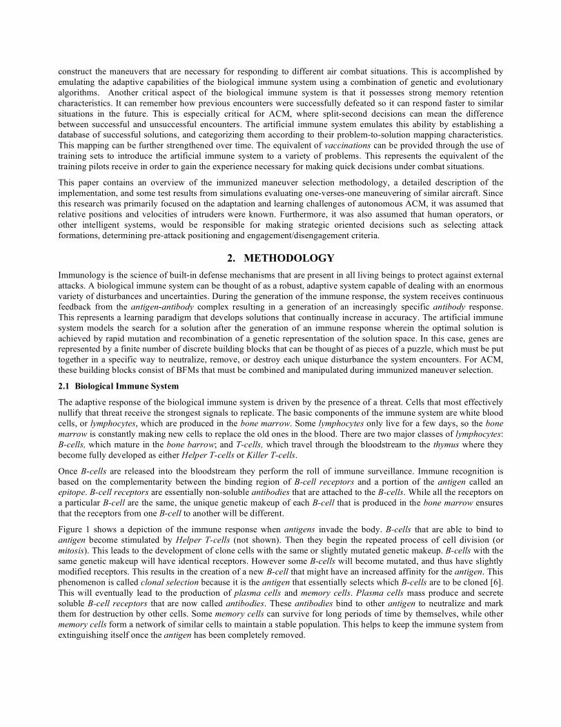
Figure 2 contains a system level diagram of the artificial immune system’s computational models, along with the a priori

knowledge that applies it to immunized maneuver selection. In terms of an immune system metaphor, intruder aircraft

can be viewed as antigens, whose epitopes are expressed in terms of their relative positions and velocities. B-cells can be

viewed as the vessels that carry the antibodies, which in turn represent maneuvers that are used in response to the threat.

Each maneuver consists of a sequence of autopilot mode and target commands, and the scheduling time for each

command. These autopilot commands represent the basic building blocks that are stored within the gene libraries. These

libraries also contain more complex BFM building blocks that have been manually constructed to provide effective

autopilot command sequences. Maneuvers are generated through the random selection and concatenation of basic and

BFM building blocks. The genetic representation of a simple maneuver with only one autopilot command is expressed in

terms of a single binary string. More complex maneuvers with multiple autopilot commands are expressed in terms of

multiple binary strings that are linked together.

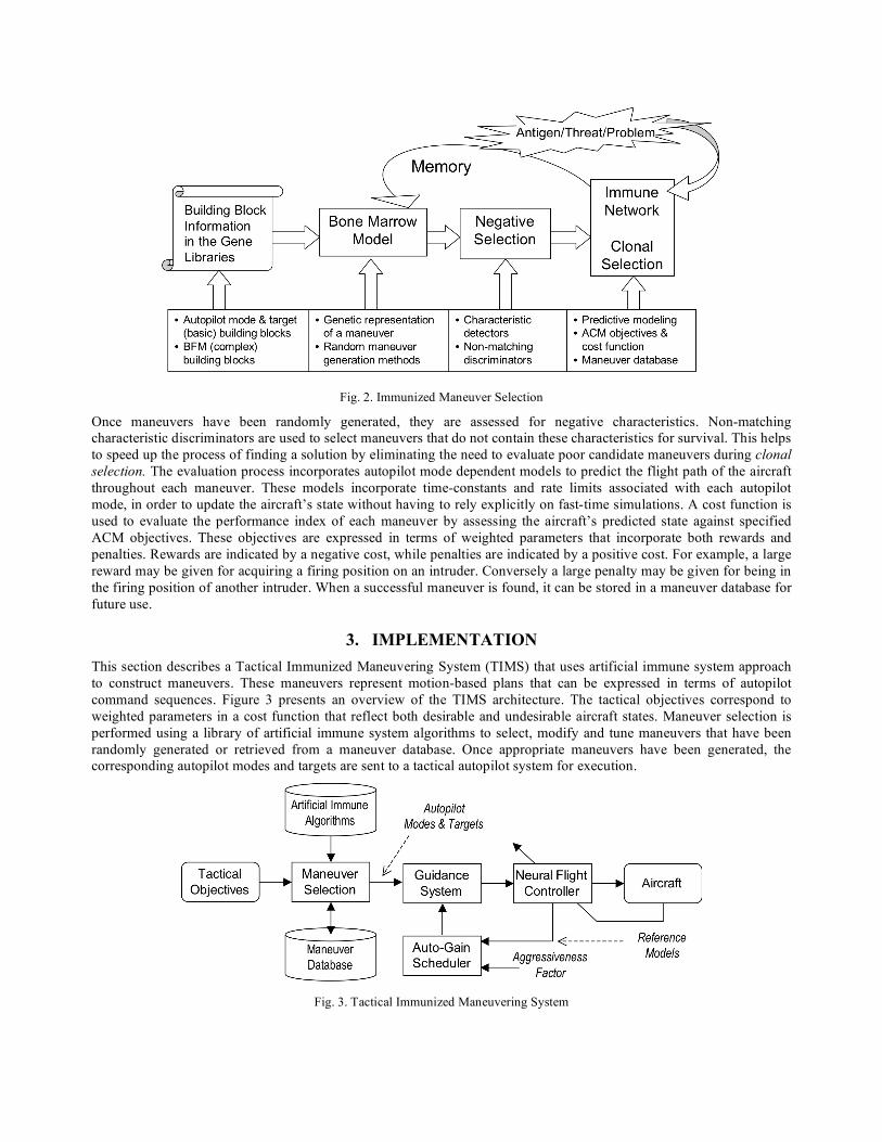
Fig. 2. Immunized Maneuver Selection

Once maneuvers have been randomly generated, they are assessed for negative characteristics. Non-matching

characteristic discriminators are used to select maneuvers that do not contain these characteristics for survival. This helps

to speed up the process of finding a solution by eliminating the need to evaluate poor candidate maneuvers during clonal

selection. The evaluation process incorporates autopilot mode dependent models to predict the flight path of the aircraft

throughout each maneuver. These models incorporate time-constants and rate limits associated with each autopilot

mode, in order to update the aircraft’s state without having to rely explicitly on fast-time simulations. A cost function is

used to evaluate the performance index of each maneuver by assessing the aircraft’s predicted state against specified

ACM objectives. These objectives are expressed in terms of weighted parameters that incorporate both rewards and

penalties. Rewards are indicated by a negative cost, while penalties are indicated by a positive cost. For example, a large

reward may be given for acquiring a firing position on an intruder. Conversely a large penalty may be given for being in

the firing position of another intruder. When a successful maneuver is found, it can be stored in a maneuver database for

future use.

3. IMPLEMENTATION

This section describes a Tactical Immunized Maneuvering System (TIMS) that uses artificial immune system approach

to construct maneuvers. These maneuvers represent motion-based plans that can be expressed in terms of autopilot

command sequences. Figure 3 presents an overview of the TIMS architecture. The tactical objectives correspond to

weighted parameters in a cost function that reflect both desirable and undesirable aircraft states. Maneuver selection is

performed using a library of artificial immune system algorithms to select, modify and tune maneuvers that have been

randomly generated or retrieved from a maneuver database. Once appropriate maneuvers have been generated, the

corresponding autopilot modes and targets are sent to a tactical autopilot system for execution.

Fig. 3. Tactical Immunized Maneuvering System

The tactical autopilot system is based upon a neural flight controller and auto-gain scheduling guidance system [9].

However, this autopilot has been enhanced with additional body-axis modes and an aggressiveness factor for enabling

high performance maneuvers. The command interface has also been modified to process mode and target sequences. The

direct adaptive tracking neural flight controller provides consistent handling qualities, across flight conditions and for

different aircraft configurations. The guidance system takes advantage of the consistent handling qualities in order to

achieve deterministic outer-loop performance. Automatic gain-scheduling is performed using frequency separation,

which is based on the natural frequencies of the neural flight controller’s specified reference models. The aggressiveness

factor is used to limit the percentage of allowable stick and pedal deflections that the guidance system can command.

These limits are then propagated throughout the guidance system in the form of computed gains and command limits.

3.1 Maneuver Prediction

During BFMs, the actions pilots take can be approximated by piece-wise linear or piece-wise constant commands, and

the switching between commands [10]. The interconnection of a finite number of commands can be used to generate

motion-based plans that can exploit the full maneuvering capabilities of the aircraft [11]. As a result, BFMs can be

represented by sequences of autopilot mode and target commands and the time to wait after each command is executed.

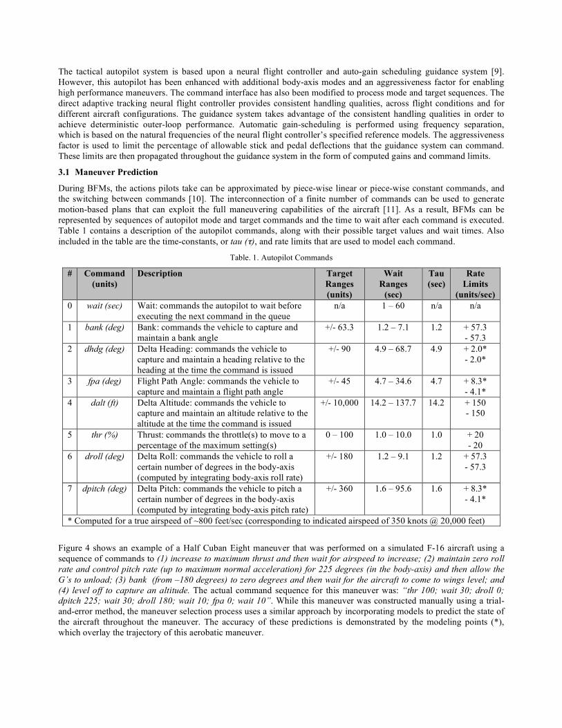
Table 1 contains a description of the autopilot commands, along with their possible target values and wait times. Also

included in the table are the time-constants, or tau (!), and rate limits that are used to model each command.

Table. 1. Autopilot Commands

# Command

(units)

Description Target

Ranges

(units)

Wait

Ranges

(sec)

Tau

(sec)

Rate

Limits

(units/sec)

0 wait (sec) Wait: commands the autopilot to wait before

executing the next command in the queue

n/a 1 – 60 n/a n/a

1 bank (deg) Bank: commands the vehicle to capture and

maintain a bank angle

+/- 63.3 1.2 – 7.1 1.2 + 57.3

- 57.3

2 dhdg (deg) Delta Heading: commands the vehicle to

capture and maintain a heading relative to the

heading at the time the command is issued

+/- 90 4.9 – 68.7 4.9 + 2.0*

- 2.0*

3 fpa (deg) Flight Path Angle: commands the vehicle to

capture and maintain a flight path angle

+/- 45 4.7 – 34.6 4.7 + 8.3*

- 4.1*

4 dalt (ft) Delta Altitude: commands the vehicle to

capture and maintain an altitude relative to the

altitude at the time the command is issued

+/- 10,000 14.2 – 137.7 14.2 + 150

- 150

5 thr (%) Thrust: commands the throttle(s) to move to a

percentage of the maximum setting(s)

0 – 100 1.0 – 10.0 1.0 + 20

- 20

6 droll (deg) Delta Roll: commands the vehicle to roll a

certain number of degrees in the body-axis

(computed by integrating body-axis roll rate)

+/- 180 1.2 – 9.1 1.2 + 57.3

- 57.3

7 dpitch (deg) Delta Pitch: commands the vehicle to pitch a

certain number of degrees in the body-axis

(computed by integrating body-axis pitch rate)

+/- 360 1.6 – 95.6 1.6 + 8.3*

- 4.1*

* Computed for a true airspeed of ~800 feet/sec (corresponding to indicated airspeed of 350 knots @ 20,000 feet)

Figure 4 shows an example of a Half Cuban Eight maneuver that was performed on a simulated F-16 aircraft using a

sequence of commands to (1) increase to maximum thrust and then wait for airspeed to increase; (2) maintain zero roll

rate and control pitch rate (up to maximum normal acceleration) for 225 degrees (in the body-axis) and then allow the

G’s to unload; (3) bank (from –180 degrees) to zero degrees and then wait for the aircraft to come to wings level; and

(4) level off to capture an altitude. The actual command sequence for this maneuver was: “thr 100; wait 30; droll 0;

dpitch 225; wait 30; droll 180; wait 10; fpa 0; wait 10”. While this maneuver was constructed manually using a trial-

and-error method, the maneuver selection process uses a similar approach by incorporating models to predict the state of

the aircraft throughout the maneuver. The accuracy of these predictions is demonstrated by the modeling points (*),

which overlay the trajectory of this aerobatic maneuver.

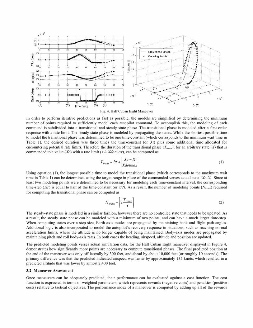
Fig. 4. Half Cuban Eight Maneuver

In order to perform iterative predictions as fast as possible, the models are simplified by determining the minimum

number of points required to sufficiently model each autopilot command. To accomplish this, the modeling of each

command is subdivided into a transitional and steady state phase. The transitional phase is modeled after a first order

response with a rate limit. The steady state phase is modeled by propagating the states. While the shortest possible time

to model the transitional phase was determined to be one time-constant (which corresponds to the minimum wait time in

Table 1), the desired duration was three times the time-constant (or 3!) plus some additional time allocated for

encountering potential rate limits. Therefore the duration of the transitional phase (Ttrans), for an arbitrary state (X) that is

commanded to a value (Xc) with a rate limit (+/- Xdotmax), can be computed as

!

Ttrans

= 3" +Xc # X

Xdotmax (1)

Using equation (1), the longest possible time to model the transitional phase (which corresponds to the maximum wait

time in Table 1) can be determined using the target range in place of the commanded verses actual state (Xc-X). Since at

least two modeling points were determined to be necessary for modeling each time-constant interval, the corresponding

time-step ("T) is equal to half of the time-constant (or !/2). As a result, the number of modeling points (Ntrans) required

for computing the transitional phase can be computed as

!

Ntrans

= 2Ttrans

"

#

$ $ %

& & (2)

The steady-state phase is modeled in a similar fashion, however there are no controlled state that needs to be updated. As

a result, the steady state phase can be modeled with a minimum of two points, and can have a much larger time-step.

When computing states over a step-size, Earth-axis modes are propagated by maintaining bank and flight path angles.

Additional logic is also incorporated to model the autopilot’s recovery response in situations, such as reaching normal

acceleration limits, where the attitude is no longer capable of being maintained. Body-axis modes are propagated by

maintaining pitch and roll body-axis rates. In both cases the heading, airspeed, altitude and position are updated.

The predicted modeling points verses actual simulation data, for the Half Cuban Eight maneuver displayed in Figure 4,

demonstrates how significantly more points are necessary to compute transitional phases. The final predicted position at

the end of the maneuver was only off laterally by 300 feet, and ahead by about 10,000 feet (or roughly 10 seconds). The

primary difference was that the predicted indicated airspeed was faster by approximately 135 knots, which resulted in a

predicted altitude that was lower by almost 2,400 feet.

3.2 Maneuver Assessment

Once maneuvers can be adequately predicted, their performance can be evaluated against a cost function. The cost

function is expressed in terms of weighted parameters, which represents rewards (negative costs) and penalties (positive

costs) relative to tactical objectives. The performance index of a maneuver is computed by adding up all of the rewards

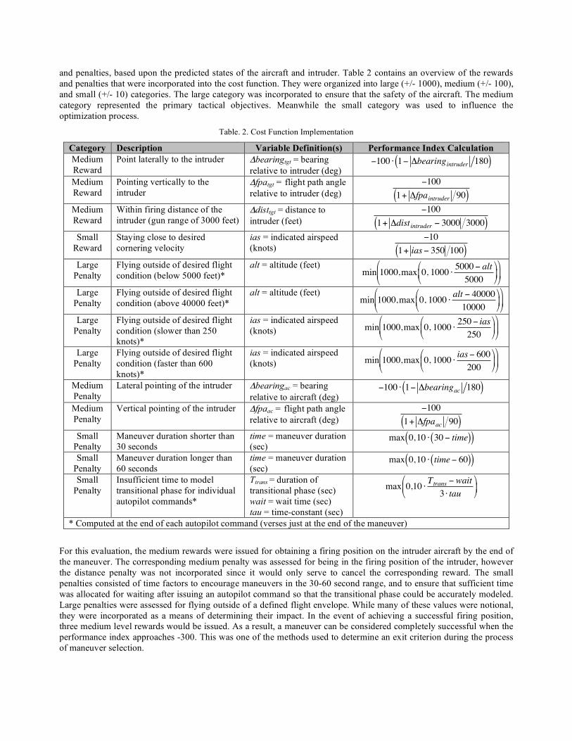
and penalties, based upon the predicted states of the aircraft and intruder. Table 2 contains an overview of the rewards

and penalties that were incorporated into the cost function. They were organized into large (+/- 1000), medium (+/- 100),

and small (+/- 10) categories. The large category was incorporated to ensure that the safety of the aircraft. The medium

category represented the primary tactical objectives. Meanwhile the small category was used to influence the

optimization process.

Table. 2. Cost Function Implementation

Category Description Variable Definition(s) Performance Index Calculation

Medium

Reward

Point laterally to the intruder "bearingtgt = bearing

relative to intruder (deg)

!

"100 # 1" $bearingintruder 180( )

Medium

Reward

Pointing vertically to the

intruder

"fpatgt = flight path angle

relative to intruder (deg)

!

"100

1+ #fpaintruder 90( )

Medium

Reward

Within firing distance of the

intruder (gun range of 3000 feet)

"disttgt = distance to

intruder (feet)

!

"100

1+ #distintruder

" 3000 3000( )

Small

Reward

Staying close to desired

cornering velocity

ias = indicated airspeed

(knots)

!

"10

1+ ias" 350 100( )

Large

Penalty

Flying outside of desired flight

condition (below 5000 feet)*

alt = altitude (feet)

!

min 1000,max 0, 1000 "5000# alt

5000

$

% &

'

( )

$

% &

'

( )

Large

Penalty

Flying outside of desired flight

condition (above 40000 feet)*

alt = altitude (feet)

!

min 1000,max 0, 1000 "alt # 40000

10000

$

% &

'

( )

$

% &

'

( )

Large

Penalty

Flying outside of desired flight

condition (slower than 250

knots)*

ias = indicated airspeed

(knots)

!

min 1000,max 0, 1000 "250# ias

250

$

% &

'

( )

$

% &

'

( )

Large

Penalty

Flying outside of desired flight

condition (faster than 600

knots)*

ias = indicated airspeed

(knots)

!

min 1000,max 0, 1000 "ias# 600

200

$

% &

'

( )

$

% &

'

( )

Medium

Penalty

Lateral pointing of the intruder "bearingac = bearing

relative to aircraft (deg)

!

"100 # 1" $bearingac 180( )

Medium

Penalty

Vertical pointing of the intruder "fpaac = flight path angle

relative to aircraft (deg)

!

"100

1+ #fpaac 90( )

Small

Penalty

Maneuver duration shorter than

30 seconds

time = maneuver duration

(sec)

!

max 0,10 " 30# time( )( )

Small

Penalty

Maneuver duration longer than

60 seconds

time = maneuver duration

(sec)

!

max 0,10 " time# 60( )( )

Small

Penalty

Insufficient time to model

transitional phase for individual

autopilot commands*

Ttrans = duration of

transitional phase (sec)

wait = wait time (sec)

tau = time-constant (sec)

!

max 0,10 "Ttrans

# wait

3 " tau

$

% &

'

( )

* Computed at the end of each autopilot command (verses just at the end of the maneuver)

For this evaluation, the medium rewards were issued for obtaining a firing position on the intruder aircraft by the end of

the maneuver. The corresponding medium penalty was assessed for being in the firing position of the intruder, however

the distance penalty was not incorporated since it would only serve to cancel the corresponding reward. The small

penalties consisted of time factors to encourage maneuvers in the 30-60 second range, and to ensure that sufficient time

was allocated for waiting after issuing an autopilot command so that the transitional phase could be accurately modeled.

Large penalties were assessed for flying outside of a defined flight envelope. While many of these values were notional,

they were incorporated as a means of determining their impact. In the event of achieving a successful firing position,

three medium level rewards would be issued. As a result, a maneuver can be considered completely successful when the

performance index approaches -300. This was one of the methods used to determine an exit criterion during the process

of maneuver selection.

3.3 Maneuver Selection

The genetic representation of an autopilot command is expressed in terms of a binary string, which is stored in a 32-bit

word. Three bits (24-27) are used to identify eight autopilot command #’s (in Table 1). The target and wait ranges for

each command (also in Table 1) are divided into eight different regions. Three bits (20-22) are used to identify the target

regions, and three bits (16-18) are used to identify the wait regions. Finally, each region is subdivided into 256 different

parts to provide the necessary resolution for computing precise target values and wait times. Eight bits (8-15) are used to

express the precision factor for each target region, and eight bits (0-7) are used to express the precision factor for each

wait region. The remaining seven spare bits are ignored.

Once the binary string for an autopilot command has been established, it can be linked with other binary strings to form

more complex maneuvers. For this evaluation, a maximum of 10 autopilot commands were allowed per maneuver. The

maneuvers were constructed through the random generation and concatenation of autopilot commands and manually

constructed BFMs. Only a select number of BFMs were constructed for this evaluation. Table 3 contains a sample of the

BFMs, along with their corresponding genetic representations.

Table. 3. Sample Basic Flight Maneuvers

Name Command Genetic Representation

Right S-Turn

(flat scissor)

bank 60; wait 4.7; wait 5.0; bank -60;

wait 4.7

00000001011101000100111101001010

00000000000000000000000000110110

00000001000001000001010101001010

Split-S droll 180; wait 6.8; dpitch 180; wait 26.5 00000110011101010110010001000000

00000111011000100000000000001100

Left Horizontal Turn

(low yo-yo)

droll -90; wait 5.2; dpitch 90; wait 15.7;

droll 135; wait 6.0; dpitch 45; wait 10.3

00000110001001000000000000000011

00000111010100010000000000010100

00000110011101000000000001010100

00000111010000000011001001001010

CW Vertical Turn

(high yo-yo)

dpitch 90; wait 15.7; droll 90; wait 5.2;

dpitch 180; wait 26.5; droll 90; wait 5.2;

dpitch 90; wait 15.7; droll 90; wait 5.2

00000111010100010000000000010100

00000110011001000000000000000011

00000111011000100000000000001100

00000110011001000000000000000011

00000111010100010000000000010100

00000110011001000000000000000011

1/3 CCW Oblique Turn

(rolling scissor)

dpitch 45; wait 10.3; droll -120; wait 5.7; 00000111010000000011001001001010

00000110000101000010000100110101

For this evaluation, a population of 100 maneuvers was initially selected and maintained throughout the selection,

cloning and maturation processes. Unless a maneuver with an “acceptable” performance index (PI < -280) was found, a

maximum of 100 generations would be computed before returning the best available maneuver in the population.

Initial Selection Process

The initial selection process consisted of randomly generating maneuvers from autopilot commands and BFMs, and by

selecting maneuvers from the maneuver database. The maneuver database contained 500 successful maneuvers that were

generated off-line using training sets that varied the relative altitude (+/- 10000 ft), flight path angle (+/- 10 deg/sec),

heading (+/- 180 deg), distance (0-10 nm) and bearing (+/- 180 deg) of the intruder. When a successful maneuver was

found, it was placed into the database along with the corresponding relative position and velocity characteristics. Before

the maneuver database is initially accessed, the strength of each maneuver is assessed by comparing the characteristics

of the maneuver against those of the current situation. The differences are weighted and added together to compute the

corresponding strength index. These strengths are then sorted and used to randomly select maneuvers from the database,

using a normal distribution to give stronger maneuvers a higher probability of selection. To provide the greatest chance

of success, the maneuver with the best strength index is automatically inserted into the initial population. To preserve

continuity, the remaining portion of the currently executing maneuver is also placed into the initial population. Once the

maneuvers have been placed into the population, they are evaluated against the cost function and sorted according to

their performance index.

Cloning Process

During the cloning process, the bottom 25% of the population is “replaced” by offspring produced through genetic

mutation [8]. This involves using a normal distribution to randomly select maneuvers from the population. Then a copy

of each selected maneuver is subjected to: (1) the insertion of an autopilot command, randomly generated maneuver, or

maneuver selected from the maneuver database; (2) the removal of an autopilot command; (3) standard or uniform bit

level crossover operators; or (4) standard or uniform custom crossover operators. The custom crossover operators

involved the swapping of modes, target and/or wait regions, and precision factors instead of individual bits.

Maturation Process

During the maturation process, the top 10% of the population is matured through random evolution. This involved

subjecting a copy of a maneuver to the random replacement of target and/or wait regions, or precision factors for each

autopilot command in the maneuver. Then the maneuver is evaluated and compared against the original maneuver. If

there is an improvement in the performance index, then the original maneuver is replaced.

Re-Selection Process

During the re-selection process, the middle 65% of the population is at risk of being replaced by “newcomers” that are

generated in a fashion that is similar to initial selection. The primary difference is that the newly generated maneuvers

have to survive the process of negative selection. This is accomplished by evaluating the performance of each new

maneuver to determine whether or not they exceed the performance of the bottom 25% of the population. Maneuvers

that would fall into the bottom 25% category are deleted. This is because they would have little chance of survival

beyond the next cloning process. However, maneuvers that would not fall into the bottom 25% category survive by

replacing one of the maneuvers in the middle 65% of the population. This is performed even if the new maneuver does

not exceed the performance of the maneuver it is going to replace. This is because the addition of the new maneuver can

provide a level of diversity into the population.

4. RESULTS

Simulation tests were performed to evaluate one-verses-one maneuvering of similar aircraft using a high fidelity model

of an F-16 aircraft [12]. The aircraft was initialized flying straight and level at an altitude of 20,000 feet and with an

indicated airspeed of 350 knots. A Dryden turbulence model was used to provide light turbulence with RMS and

bandwidth values representative of those specified in Military Specifications Mil-Spec-8785 D of April 1989. The Earth

atmosphere was based on a 1976 standard atmosphere model.

4.1 Convergence Test

One of the driving factors behind the selection of the population size and number of generations to compute was so that

solutions could be found within 1-2 seconds. To ensure that the specified number of generations was sufficient, the rate

of convergence in the population was evaluated. Figure 5 demonstrates the results from one of the more difficult

convergence tests, where the aircraft was initialized far away from the intruder so that the performance index was less

responsive to differences between maneuvers.

Fig. 5. Convergence Test

The best performance index (Best PI) in the population converges quickly to a solution, and appears to go through a

slight maturation process after 40 iterations. This may be an indication that the number of generations could potentially

be decreased even further. However, the performance index that is used as the cutoff point for negative selection (Cutoff

PI) also converges very quickly. This may be an indication that there is not enough diversity in the population, since

only a few randomly generated maneuvers manage to survive the process of negative selection after 20 iterations.

4.2 Static Tests

Monte Carlo testing was perfomed in order to evaluate the effectiveness and accuracy of the maneuvers. Test cases

consisted of the same intruder flying eastwards, straight and level at 20000 feet. The aircraft was also initialized flying

straight and level, but in random directions and at different positions and altitudes around the intruder. Figure 6 presents

10 test cases that demonstrate the effectiveness of the predicted maneuvers. However, in some test cases (such as #7) the

prediction does not match the simulated trajectory. This is especially problematic for situations where the aircraft pitches

up beyond 90 degrees (as in the Half Cuban Eight maneuver), where insufficient airspeed can result in unmodeled

dynamics that can significantly alter the final state. Table 4 contains the maneuver commands for each test case.

Fig. 6. Static Tests

Table. 4. Maneuver Commands Generated during Static Tests

Test Case Command

1 bank -61.88; wait 4.98; wait 30.20; fpa -6.30; wait 21.96

2 bank 60.93; wait 6.04; droll 175.50; wait 9.22; dpitch 297.00; wait 37.38

3 bank 37.66; wait 6.20; wait 53.58

4 bank 59.98; wait 3.96; fpa 6.19; wait 27.49; thr 75.00; wait 8.68 fpa -42.75; wait 19.88

5 dpitch 269.10; wait 32.87

6 thr 7.00; wait 3.63; bank 63.30; wait 6.84; wait 39.50 7 dpitch 196.20; wait 51.86; bank 61.72; wait 7.27 8 dbank 62.83; wait 6.29; wait 30.20; fpa 8.55; wait 22.22 9 bank -21.21; wait 6.17; wait 20.03; bank 33.23; wait 6.04; fpa -4.61; wait 27.04 10 fpa -10.12; wait 33.33; fpa 28.12; wait 26.60

4.3 Dynamic Tests

Dynamic testing was performed by allowing maneuvers to be re-computed every five seconds, in response to changes in

the intruder’s trajectory. During the lateral tests, the intruder performed a series of (60 deg) bank maneuvers in an

approximation of the “flat scissors” technique. During the coupled (lateral and vertical) tests, the intruder performed a

series of (60 deg) bank and (5 deg) flight path angle maneuvers, in a pseudo approximation of the “rolling scissors”

technique. Figure 7 presents results from a lateral test case (on the left), and a coupled test case (on the right). In both

cases, circles have been placed at 5-second intervals along the trajectories. In general, the lateral tests were found to

produce fairly deterministic results. However, the coupled tests often resulted in vertical overshoots caused by over

aggressiveness. This could potentially be traced back to the lack of derivative terms in the cost function.

Fig. 7. Dynamic Tests

5. CONCLUSIONS

The purpose of this study was to evaluate the effectiveness of using an artificial immune system approach for ACM. Test

results demonstrate the potential of immunized maneuver selection, in terms of constructing effective motion-based

trajectories over a relatively short (1-2 sec) period of time. In most cases, the trajectories were adequately predicted with

minimal computation to enable iterative calculations. However, further research is still required in terms of improving

the cost function implementation, and tuning convergence rates so that a diverse population is maintained. Additional

development is also necessary to improve aspects of the predictive modeling, and to manage the execution of

recalculated maneuvers during real-time operation.

REFERENCES

1. KrishnaKumar, K., Kaneshige, J., and Satyadas, A., “Challenging Aerospace Problems for Intelligent Systems,”

Proceedings of the von Karman Lecture series on Intelligent Systems for Aeronautics, Belgium, May 2002.

2. Review of ONR’s Uninhabited Combat Air Vehicles Program, National Academy Press, Washington D.C., 2000.

3. Allen Moshfegh, Office of Naval Research, Basic Research Programs on Intelligent Autonomous Agents, briefing

presented to the committee, December 13, 1999.

4. http://en.wikipedia.org/wiki/Air_combat_manoeuvering

5. Robert L. Shaw, Fighter Combat Tactics and Maneuvering, Naval Institute Press Annapolis, Maryland, 1985.

6. http://users.rcn.com/jkimball.ma.ultranet/BiologyPages/C/ClonalSelection.html

7. Krishnakumar, K., “Artificial Immune System Approaches for Aerospace Applications,” AIAA-2003-0457

8. http://en.wikipedia.org/wiki/Crossover_(genetic_algorithm)

9. Kaneshige, John, John Bull, and Joseph J. Totah, Generic Neural Flight Control and Autopilot System, AIAA 2000-

4281, August 2000.

10. Gavrilets, V., I. Martinos, B. Mettler, and E. Feron, Flight Tests and Simulation Results for an Autonomous

Aerobatic Helicopter, Proceedings of the 21st Digital Avionics Systems Conference (8C3), Irvine, CA, October

2002.

11. Frazzoli, E., Maneuver-Based Motion Planning and Coordination for Multiple UAV’s, Proceedings of the 21st

Digital Avionics Systems Conference (8D3), Irvine, CA, October 2002.

12. http://www.aem.umn.edu/people/faculty/balas/darpa_sec/SEC.Software.html