Article Post-Print The following article is a “post-print” of an article accepted for publication

in an Elsevier journal.

The post-print is not the final version of the article. It is the version which

has been accepted for publication after peer review, but before it has gone

through the editing process with the publisher. Therefore, there may be

differences with this version and the final version.

The final, official version of the article can be downloaded from the

journal’s website via this DOI link when it becomes available (subscription

or purchase may be required):

DOI: 10.1016/j.cep.2015.07.002 (2015)

This post-print has been archived on the author’s personal website

(macc.mcmaster.ca) in compliance with the National Sciences and

Engineering Research Council (NSERC) policy on open access and in

compliance with Elsevier’s academic sharing policies.

This post-print is released with a Creative Commons Attribution Non-

Commercial No Derivatives License.

Date Archived: July 2, 2015

1

Title: Design of dividing wall columns for butanol recovery in a thermochemical

biomass to butanol process

Chinedu O. Okoli and Thomas A. Adams II*

Department of Chemical Engineering, McMaster University, 1280 Main Street West,

Hamilton, Ontario

Abstract

In this work, ternary and quaternary dividing wall column (DWC) configurations for the

separation of a multicomponent feed stream from a novel thermochemical

lignocellulosic biomass to butanol process are designed, modeled and assessed. The

goal is to separate the feed into four major products, with a key product being a

biobutanol rich stream. Due to the complexity of DWC models, a shortcut modeling

approach based on the minimum energy mountain method (also called the “V min

diagram method”) is used to determine good initial values for the decision variables for

the rigorous simulation of the DWC configurations. Furthermore, each DWC

configuration is optimized to minimize the total annualized cost with the use of a

derivative free algorithm coupled with a process simulator. The results show that the

quaternary DWC configuration achieves up to 31 % energy savings, and 15 % capital

savings in comparison to a conventional distillation sequence, and is thus a better option

for implementation in the biofuel process.

* Corresponding author: Email: tadams@mcmaster.ca; Ph: (905) 525-9140 x24782

DWC, dividing wall columns; GA, genetic algorithm; HK, heavy key; LK, light key; MESH, material equilibrium summation and

heat; MINLP, Mixed Integer Nonlinear Programming; NRTL, non-random two-liquid; PSO, particle swarm optimization; TAC,

total annualized cost; VBA, Visual Basic for Applications; VLE, vapor liquid equilibrium; Vmin, minimum energy mountain

*ManuscriptClick here to view linked References

2

Keywords: dividing wall column; biobutanol; Vmin diagram; acyclic simulation

structure; particle swarm optimization; total annualized cost

1. Introduction

As a result of global efforts to reduce emissions related to fossil fuel consumption, there

has been a shift of focus to produce fuels from biomass. For example, the contribution

of biofuels to total road-transport fuel demand was 3 % in 2013 and is estimated to grow

to 8 % by 2035 [1]. However, to encourage further increase in the uptake of biofuels,

production costs have to be reduced. One way to address this challenge is to reduce

biofuel processing costs by employing cutting edge process intensification technologies

such as dividing wall columns (DWC).

Since its first industrial application in 1985 by BASF, there have been more than one

hundred DWCs implemented in industry, highlighting its increasing popularity [2], with

past research showing that DWCs can reduce the investment and energy consumption of

a multicomponent distillation process by up to 30 % in comparison to conventional

distillation sequences [3–5].

Though DWC technology initially found wide application for distillation of zeotropic

mixtures, its use has been further extended to other areas such as extractive distillation

[6,7], azeotropic distillation [7,8] and reactive distillation [7]. Also critical to this uptake

of DWCs is the fact that questions surrounding the controllability and operability of 3-

product and 4-product DWCs have largely been addressed [4,9–12].

One important biofuel production process which may potentially benefit from the

application of DWC technology is biobutanol production. This is because biobutanol, a

gasoline substitute, is gathering increasing attention due to its advantages over

bioethanol [13,14]. Recently, Okoli and Adams [15] showed that the fuel can be

3

produced at a cost of $0.83/L using a novel thermochemical process. That process used

a train of conventional distillation columns in the separation section to separate an

eleven component feed into four product blends (including a fuel-grade biobutanol

product), and consumed 10% of the total energy and 8% of the total direct costs of the

process. However, these energy and capital costs of the separation section can

potentially be improved by utilizing DWCs for biobutanol recovery instead of

conventional distillation columns, leading to a reduction in production costs of the

process and thus have a significant impact in improving the competitiveness of

biobutanol as a gasoline replacement. This application of DWC technology has not been

previously investigated for biobutanol recovery from a thermochemical process, and is

an interesting area of research as past research has demonstrated the benefits of DWC

applications to bioethanol, bioDME and biodiesel production processes [16,17].

One major challenge in the research of DWC applications is their design. In commercial

chemical process simulators the modeling of a DWC can be a difficult task as there are

no custom DWC blocks. Methods identified from literature have made use of multiple

columns in process simulators to represent different sections of the DWC [18,19].

Another challenge is the large number of internal column specifications needed for a

DWC. This complexity means that computational difficulties should be avoided by

using appropriate short-cut methods to determine initial estimates for the variables

required for rigorous simulations. Once these variables have been estimated, rigorous

simulations based on tray-by-tray MESH (material, equilibrium, summation and heat)

equations can be implemented in the process simulation software. One such short-cut

method is the minimum energy mountain method (also called the "Vmin diagram

method"). The Vmin diagram method is a distillation column design tool that can be

adapted and used to obtain good estimates for initializing rigorous DWC simulations. It

4

provides a graphical visualization of the minimum energy required for separation of a

multicomponent zeotropic feed as a function of the feed properties [20]. The minimum

energy is represented by the normalized vapor flow in the top section of the column,

with the highest peak representing the minimum theoretical energy required for

separation. The concept of the Vmin diagram was introduced by Halvorsen and

Skogestad of the Norwegian University of Science and Technology (NTNU) in a series

of papers in 2003 [20–22]. The method was developed based on Underwood's

equations, and requires only input feed details such as feed flowrate (F), composition (z)

and feed quality (q) to estimate the minimum vapor flow in the top section of the

column (VT), and distillate (D) at infinite number of trays for desired product recoveries.

The method can also be used to generate initial estimates for nonideal systems by using

a process simulator and a large number of trays, typically around four times the

minimum number of trays (Nmin) [20].

Outside NTNU, this method has only been applied to the design of 4-product DWCs for

multicomponent aromatics mixtures [19,23] and Sun and Bi [24] to the conceptual

design of 3-product reactive DWCs. These papers demonstrated the efficacy of this

method. However, as the number of applications of this method is limited, more

independent validations are needed to demonstrate its potential.

In process design, the comparison of different design options is usually done based on

identical criteria after an optimization has been carried out. Classical methods for

optimizing DWCs are based on mathematical programming (which require derivative

information) and fall into a class of problems known as Mixed Integer Nonlinear

Programming (MINLP) problems. This is due to the presence of discrete variables such

as feed location, and number of trays in different column sections, as well as the

nonconvexity of the MESH equations. Javaloyes-Anton et al. [25], reviewed the

5

application of MINLP formulations for the solutions of complex distillation columns

(including DWCs), and concluded that based on the high nonlinearities of these

formulations, as well as sophisticated initialization techniques needed to obtain feasible

solutions (only local optima are guaranteed as the solutions are highly dependent on the

initialization points), these methods are complex and suited only for those skilled

enough to adapt them for their own requirements.

An alternative, and easier to implement approach to these methods is to leverage the use

of commercial process simulators and derivative-free or "black box" optimization

algorithms. These derivative-free algorithms are typically population based, wherein the

population contains individuals, with each individual representing a particular solution

to the optimization problem. Once an algorithm termination criterion has been reached

the optimization problem solution is chosen as that of the individual with the best

objective function value. The advantage of these algorithms over derivative search

methods is their ability to escape local optima and infeasibility regions, as well as

provide multiple feasible solutions to account for real world considerations that are

harder to quantify by the designer in an optimization setting. However, they are not able

to guarantee that the solutions found are optimal. Though derivative-based search

methods can theoretically offer local optimality guarantees, they are not easily amenable

to highly complex real world problems and might be unable to find solutions which are

as good as those obtained by derivative-free algorithms [25,26]. Examples of these

derivative-free algorithms include genetic algorithms (GA), simulated annealing,

particle swarm optimization (PSO) amongst others. In-depth discussions about these

methods can be found in books, such as those written by Gendreau and Potvin [27], and

Kaveh [28].

6

As a result of these advantages of derivative-free optimization algorithms over classical

derivative search methods, the use of derivative-free optimization algorithms coupled

with process simulators has found wide use in the literature for optimizing complicated

process systems [25]. Amongst many examples in literature, Leboreiro and Acevedo

[26] successfully demonstrated the use of a modified GA interconnected with the Aspen

Plus process simulator to optimize complex distillation sequences including a Petlyuk

column. Pascall and Adams II [29] made use of a PSO algorithm connected to Aspen

Dynamics to optimize a novel semicontinuous system for the separation of DME from

methanol and water. In that work PSO was used to optimize the controller tuning

parameters of the system. The PSO algorithm coupled with Aspen Hysys was used by

Javaloyes-Anton et al. [25] for the optimal design of conventional and complex

distillation processes. In their work, the PSO algorithm implemented in MATLAB

handles all the discrete variables such as the feed location and the number of trays in

column sections, while continuous variables (reflux ratio, boilup ratio etc.) and product

purity specifications are handled at the process simulator level. An interesting feature of

their work was the use of a novel acyclic DWC simulation structure proposed by

Navarro et al. [30] for representing a 3-product DWC in the process simulator. The use

of an acyclic simulation structure over a traditional recycle structure reduces the

simulation time in the process simulator, as the convergence of recycle tear streams is

avoided. Despite the efficacy of their methodology, its application to DWCs was

restricted to a relatively simple Benzene-Toluene-Xylene feed.

Based on this background, the objective of this paper is to investigate the benefits of

applying 3-product and 4-product DWC technology to the recovery of fuel-grade

biobutanol from a highly non-ideal multicomponent alcohol rich feed obtained from a

thermochemical biobutanol process. The novelty of our work lies in the use of a

7

comprehensive methodology for designing the DWCs for this particular application.

Firstly, we demonstrate how the Vmin method can be used to estimate decision variables

for acyclic 3-product and more complicated 4-product DWC simulation structures in

Aspen Plus. Furthermore, the PSO algorithm coupled with Aspen Plus is then used to

optimize the DWCs to minimize an economic objective function. In addition, a

sensitivity analysis to investigate the importance of key parameters on the structure and

economics of the best DWC configuration was also performed. To the best of our

knowledge, this detailed approach for assessing and quantifying the potential for the

application of DWC technology to biobutanol recovery is the first of its kind.

The rest of the paper is written as follows. Section 2 describes the system and design

configurations under study, while in section 3 the design methodology is explained in

detail. Subsequently, the results of the designed configurations are presented and

analyzed in section 4. Finally, conclusions are drawn in section 5.

2. System Description

2.1 Feed and products

The multicomponent mixture to be separated is derived from a biobutanol synthesis

process [15]. In this process, lignocellulosic biomass is converted to mainly biobutanol

and other mixed alcohols through a number of processing steps consisting of biomass

drying, gasification, syngas cleanup, and mixed alcohol synthesis. The resulting mixture

undergoes a number of pre-distillation separation steps such as flashing to remove light

gases, and water adsorption over a molecular sieve. Separation by distillation, which is

the subject of this study, is then used to recover biobutanol and other mixed alcohols as

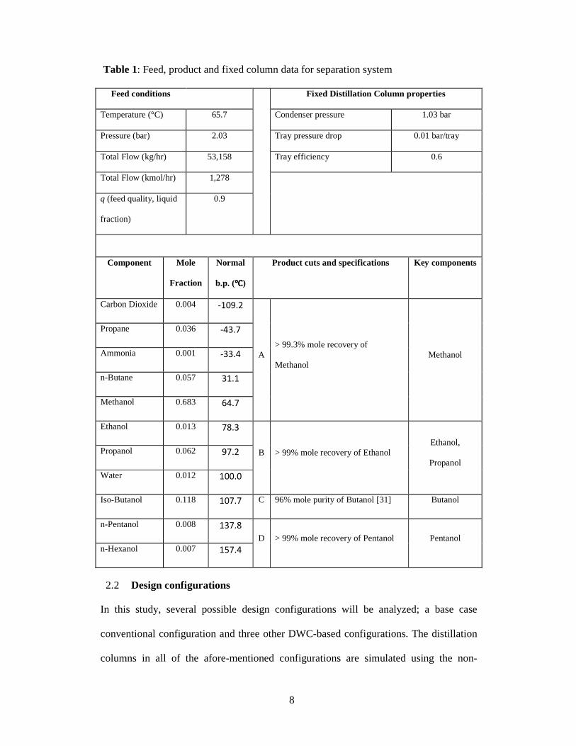
products. Table 1 shows the components and feed conditions into the distillation

system, as well as the product specifications.

8

Table 1: Feed, product and fixed column data for separation system

Feed conditions Fixed Distillation Column properties

Temperature (°C) 65.7 Condenser pressure 1.03 bar

Pressure (bar) 2.03 Tray pressure drop 0.01 bar/tray

Total Flow (kg/hr) 53,158 Tray efficiency 0.6

Total Flow (kmol/hr) 1,278

q (feed quality, liquid

fraction)

0.9

Component Mole

Fraction

Normal

b.p. ()

Product cuts and specifications Key components

Carbon Dioxide 0.004 -109.2

A > 99.3% mole recovery of

Methanol Methanol

Propane 0.036 -43.7

Ammonia 0.001 -33.4

n-Butane 0.057 31.1

Methanol 0.683 64.7

Ethanol 0.013 78.3

B > 99% mole recovery of Ethanol Ethanol,

Propanol Propanol 0.062 97.2

Water 0.012 100.0

Iso-Butanol 0.118 107.7 C 96% mole purity of Butanol [31] Butanol

n-Pentanol 0.008 137.8

D > 99% mole recovery of Pentanol Pentanol n-Hexanol 0.007 157.4

2.2 Design configurations

In this study, several possible design configurations will be analyzed; a base case

conventional configuration and three other DWC-based configurations. The distillation

columns in all of the afore-mentioned configurations are simulated using the non-

9

random, two-liquid (NRTL) activity coefficient model with the Redlich-Kwong model

for the gas phase and default binary interaction parameters provided in the simulator,

Aspen Plus V8.0.

This model was chosen because it provided a good fit to experimental data for the most

abundant alcohols (methanol to isobutanol) in the feed mixture (see Table 1).

Specifically, the binary vapor liquid equilibrium (VLE) data of the methanol-isobutanol

[32], ethanol-isobutanol [33], propanol-isobutanol [34], methanol-propanol [35],

methanol-ethanol [36], ethanol-propanol [37] pairs were validated against experimental

data. Furthermore, we note that the simulation did not detect two liquid phases using

this model for any of the columns described in this study, and that there are no

azeotropes present because of the very low water content in the feed.

2.2.1 Base case

There are five possible sequences of conventional binary distillation columns for the

separation of a multicomponent feed into four products [38]. A quick way for

identifying the most promising distillation sequence for further study is to apply the

marginal vapor rate method [39] to determine the sequence with the least vapor flow

rate. The vapor flow through the column provides a good indicator of both the column's

capital and operating costs. This is because the reboiler and condenser duties increase

with increased vapor flow, and larger vapor flows lead to larger diameter columns and

thus higher capital costs. Therefore distillation sequences with lower vapor loads are

preferred.

The results of the marginal vapor rate method as applied to the feed conditions and key

component data provided in Table 1 are shown in Fig. 1. Each configuration is designed

for 99.3 mol % recovery of key components, constant column pressure of 1 atm and a

10

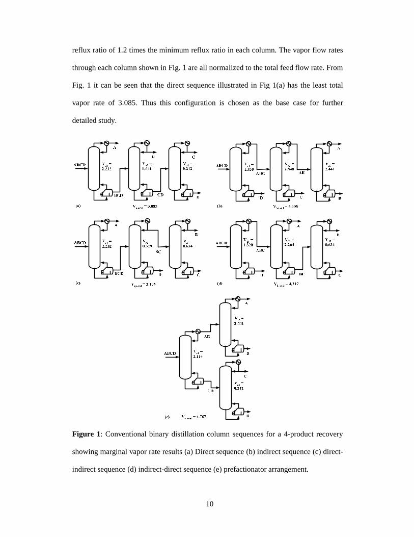
reflux ratio of 1.2 times the minimum reflux ratio in each column. The vapor flow rates

through each column shown in Fig. 1 are all normalized to the total feed flow rate. From

Fig. 1 it can be seen that the direct sequence illustrated in Fig 1(a) has the least total

vapor rate of 3.085. Thus this configuration is chosen as the base case for further

detailed study.

Figure 1: Conventional binary distillation column sequences for a 4-product recovery

showing marginal vapor rate results (a) Direct sequence (b) indirect sequence (c) direct-

indirect sequence (d) indirect-direct sequence (e) prefactionator arrangement.

11

2.2.2 DWC configurations

A DWC is a fully thermally coupled distillation sequence in which one condenser and

one reboiler are used together with a single column containing one or more longitudinal

partition walls, irrespective of the number of products required [19]. In the DWC, the

internal re-mixing of streams which occurs in conventional columns is avoided,

minimizing the entropy of mixing and thus energy required for separation of

components [19]. The use of a single shell, reboiler and condenser to perform

multicomponent (three or more components) separations in a DWC means that capital

and energy costs of a distillation process can potentially be reduced.

Figs. 2 - 4 show three DWC configurations to be analyzed in this study. In Fig. 2 a

DWC configuration with a conventional column for methanol recovery in direct

sequence with a ternary product DWC is shown, while Fig. 3 shows a DWC

configuration with a ternary product DWC in direct sequence with a butanol recovery

column. Finally, Fig. 4 (a) shows a quaternary product DWC based on the Kaibel

configuration i.e. using only a single partition wall [40]. The Kaibel configuration

generally has a higher energy requirement than a 4- product Petlyuk configuration (Fig.

4 (b)) for the same quaternary product separation. However, the Kaibel column is

preferred for practical implementation because it is easier to design, construct and

operate, while the 4-product Petlyuk configuration has mechanical design, operational

and control uncertainties that are yet to be overcome [19,41]. Therefore, the 4-product

Petlyuk configuration is not chosen for this study.

12

Figure 2: DWC configuration 1. Methanol recovery column and 3-product Petlyuk

DWC

Figure 3: DWC configuration 2. 3-product Petlyuk DWC and butanol recovery column

B

C

D

ABCD

A

CD

ABCD

A

B

D

C

A

B

D

C

ABCD

(a) (b)

13

Figure 4: 4-product DWC using (a) the Kaibel configuration; (b) the 4-product Petlyuk

configuration. The 4-product Petlyuk configuration is not used in this study except to

help synthesize the Kaibel configuration.

3. Methodology

3.1 DWC simulation structure in process simulator

In process simulators, the traditional simulation strategy for DWCs is to represent the

DWC structure as conventional columns in sequence connected by liquid-vapor recycle

streams at the top and bottom of the column. This structure is also known as a recycle

structure and is illustrated in Fig. 5 (a) for a ternary product DWC. In this structure, the

first distillation column models the prefractionator section of the DWC, while the

second column models the product sections of the DWC. In Aspen Plus, for example,

each column in the model would be one RadFrac block. There are a number of

disadvantages to this method; all related to the presence of recycle streams. The

convergence of recycle streams when using the sequential modular mode of process

simulators such as Aspen Plus is done through tear streams, thus at each iteration the

columns and tear streams have to be converged leading to longer simulation times and a

proneness to non-convergence. This is undesirable for scenarios where a flowsheet will

undergo a large number of runs and robustness is a key criteria, such as when linked to

an external optimization algorithm.

14

Figure 5: Two column structure options for the simulation of a ternary DWC: (a)

recycle structure (b) acyclic structure

An alternative model structure for DWC simulation is the acyclic structure proposed by

Navarro et al. [30], illustrated in Fig. 5 (b) for a ternary product DWC. In their work, the

authors replace the material recycle streams present in the recycle DWC structure with

material and energy streams. The top of the first column (prefractionator) is connected

to the rectifying section of the second column (main column) with a vapor material

stream at its dew point and an energy stream with the same energy that would have been

removed if a partial condenser was used to provide reflux to the prefractionator.

Furthermore, the bottom of the prefractionator is connected to the stripping section of

the main column with a liquid material stream at its bubble point and an energy stream

with the same energy that that would have been added if a reboiler was used to provide

vapor to the first column. The acyclic structure avoids the problems associated with the

presence of recycle streams in the recycle structure and thus simulates faster with easier

convergence.

15

3.2 DWC initialization (minimum energy mountain (Vmin) diagram method)

Figure 6: Example of column sections of a ternary DWC, and the Vmin diagram

The Vmin diagram method is used to generate good initial estimates of the design

parameters for the DWCs discussed in this work using the following steps:

1. Select key components and their required recoveries (99.3 mol % is used in this

study) for the given feed properties. For example from Table 1, for the separation

between cut A and cut B, methanol is the light key (LK) component while ethanol is the

heavy key (HK) component.

2. Calculate VT/F and corresponding D/F values for all possible LK and HK splits

between key components in a binary distillation column at constant pressure using at

least 4Nmin equilibrium stages at the specified recoveries. For example, to split a mixture

of ABC in a single binary distillation column, there are three possible splits. (1) A/B,

meaning that A is recovered in the distillate and B in the bottoms to the desired

recoveries; (2) B/C, meaning B (and therefore A) in the distillate and C in the bottoms;

and (3) A/C, meaning that A is in the distillate and C is in the bottoms to the desired

16

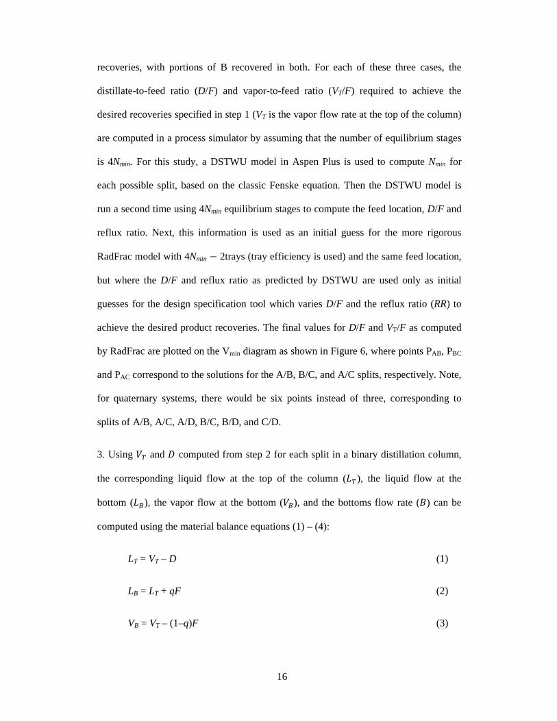
recoveries, with portions of B recovered in both. For each of these three cases, the

distillate-to-feed ratio (D/F) and vapor-to-feed ratio (VT/F) required to achieve the

desired recoveries specified in step 1 (VT is the vapor flow rate at the top of the column)

are computed in a process simulator by assuming that the number of equilibrium stages

is 4Nmin. For this study, a DSTWU model in Aspen Plus is used to compute Nmin for

each possible split, based on the classic Fenske equation. Then the DSTWU model is

run a second time using 4Nmin equilibrium stages to compute the feed location, D/F and

reflux ratio. Next, this information is used as an initial guess for the more rigorous

RadFrac model with 4Nmin − 2trays (tray efficiency is used) and the same feed location,

but where the D/F and reflux ratio as predicted by DSTWU are used only as initial

guesses for the design specification tool which varies D/F and the reflux ratio (RR) to

achieve the desired product recoveries. The final values for D/F and VT/F as computed

by RadFrac are plotted on the Vmin diagram as shown in Figure 6, where points PAB, PBC

and PAC correspond to the solutions for the A/B, B/C, and A/C splits, respectively. Note,

for quaternary systems, there would be six points instead of three, corresponding to

splits of A/B, A/C, A/D, B/C, B/D, and C/D.

3. Using and computed from step 2 for each split in a binary distillation column,

the corresponding liquid flow at the top of the column (), the liquid flow at the

bottom (), the vapor flow at the bottom (), and the bottoms flow rate () can be

computed using the material balance equations (1) – (4):

LT = VT – D (1)

LB = LT + qF (2)

VB = VT – (1–q)F (3)

17

B = F – D (4)

These flows are depicted graphically in Fig. 6 for the column sections of a ternary

DWC.

4. The corresponding operating variables such as RR and boilup ratios (BR) which are

useful for initializing the DWC simulation structure can then be computed using

equations (5) – (6), while the side flowrate(s) can be calculated via an appropriate

material balance.

RR = LT /D (5)

BR = VB /B (6)

3.3 Derivative-free Optimization algorithm

The PSO algorithm is a derivative-free optimization technique inspired by nature. The

algorithm mimics the way a swarm of birds (particles) locate a best landing place. In the

algorithm, the velocity and position of each particle in a swarm is updated iteratively

based on its (i) past velocity and position (ii) personal best position at each iteration (iii)

global best position (swarm's best) at each iteration. The algorithm is terminated once a

stopping criterion is satisfied, and the global best position is subsequently outputted as

the optimum. Adams II and Seider [42] demonstrated the effectiveness of the PSO

algorithm for the practical optimization of complex chemical distillation processes.

Apart from its effectiveness, it is also chosen for this work because it is easy to

implement and use with commercial simulation software, and has few tuning

parameters.

For this work a discrete version of the PSO algorithm in which discrete decision

variables are treated as continuous variables for use in the PSO algorithm, but rounded

18

to the nearest integer (or discrete value) when used to evaluate the objective function

(that is, to run the simulation) [43]. Furthermore, the positions of the particles are

initialized using a Latin hypercube sampling method to enable adequate sampling of the

search space.

3.4 Objective function

Table 2: Additional data for capital and utility costs calculations

Distillation columns (default values from Aspen Plus V8.0)

Tray type: sieve tray

Tray spacing, s: 0.609 m

Column height, H (m) = 3 + (NT × s); where NT = number of trays

Flooding approach: 80 % [44]

Utility costs

Natural gas [45] $2.38/GJ

Electricity [46] $0.0491/kWh

Water makeup and treatment [47] 0.0005 cents /L

Steam, computed cost (10 bar medium pressure steam, 185 °C) $2.14 /GJ

Cooling water, computed cost (30 − 45 °C) $0.278 /GJ

The basis of comparison of the design configurations is the total annualized cost (TAC)

of each design, which is minimized as the objective function of the PSO algorithm. The

TAC for each column is a sum of the operating cost per year and annualized capital cost

of the column, assuming an annualization period in years. The operating cost is the cost

of the utilities (steam and cooling water) needed to provide the required heating and

cooling duties to the column reboiler and condenser. These costs are estimated using the

method described by Towler and Sinnott [47] in which the prices of steam (medium

pressure) and cooling water are directly related to the prices of natural gas, electricity

19

and water (see Table 2 for references).The capital cost is dependent on the column

diameter, number of trays, and heat exchanger areas. Correlations for computing the

costs of the reboiler, condenser, and sieve trays are obtained from Seider et al. [38],

while cost correlations for the column are obtained from Rangaiah et al. [48]. Dejanovic

et al. [9] recommends that the sieve trays in the dividing wall section of the DWCs

should be about 1.2 times the cost of conventional sieve trays. Instead, it was assumed

that the cost is 1.5 times the cost of conventional sieve trays as a conservative estimate.

These sieve trays are specially constructed with partition walls for use in DWCs with

non-welded walls. Dejanovic et al. [9] notes that they are becoming more popular in

DWCs as they allow much more design and implementation flexibility. The material of

construction is assumed to be carbon steel for all capital cost computations. The

computed capital cost is subsequently annualized by multiplying with an annualization

factor (f) using equation (7), where i is the fractional interest rate per year, and n is the

annualization period in years. The values of i and n are set at 0.1 (or 10 %) and 5 years

respectively as recommended by Smith [49].

(7)

In order to consistently compare the predicted costs of the DWC systems in this work to

the costs of the conventional continuous distillation sequences, the cost year for the

analysis is December 2012 with an operating time of 8,000 h/yr for all cases. Other data

for the computation of the capital and utility costs are shown in Table 2.

20

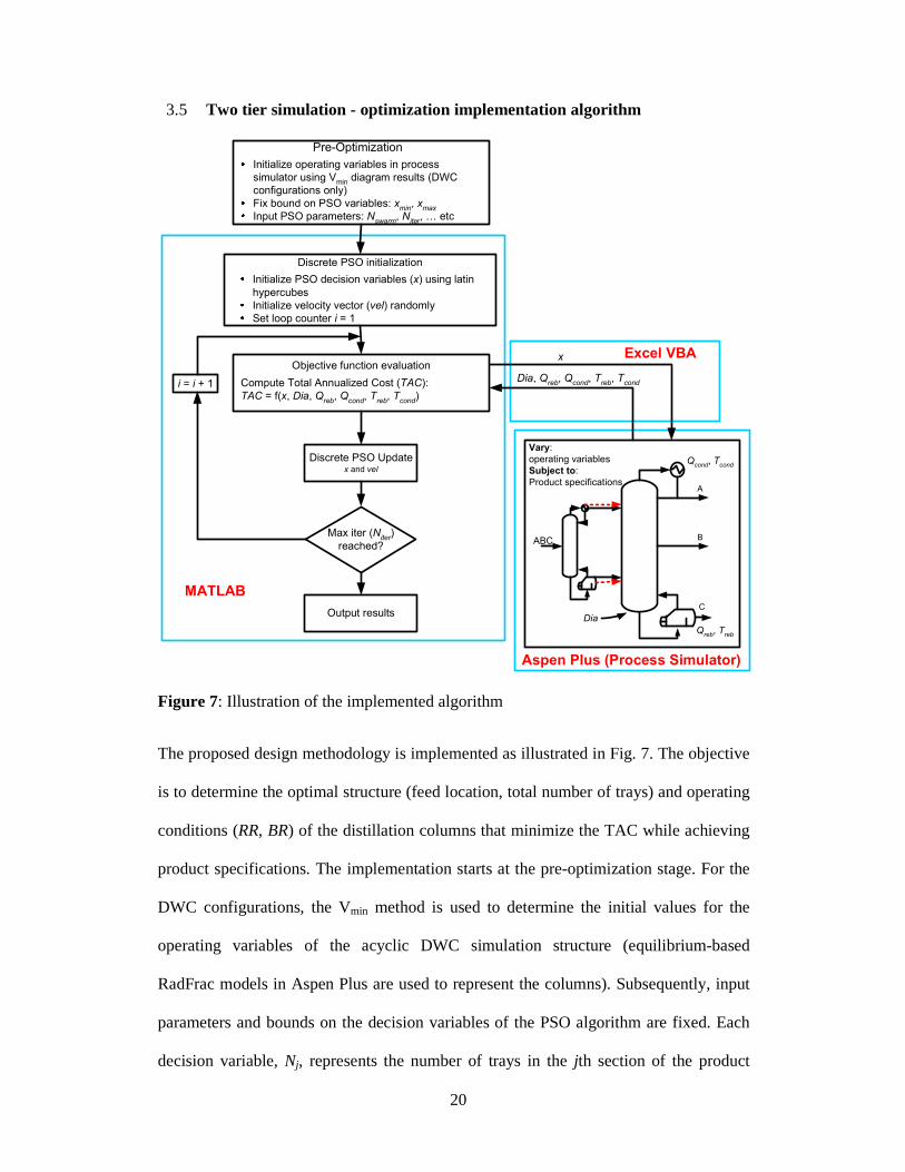
3.5 Two tier simulation - optimization implementation algorithm

Figure 7: Illustration of the implemented algorithm

The proposed design methodology is implemented as illustrated in Fig. 7. The objective

is to determine the optimal structure (feed location, total number of trays) and operating

conditions (RR, BR) of the distillation columns that minimize the TAC while achieving

product specifications. The implementation starts at the pre-optimization stage. For the

DWC configurations, the Vmin method is used to determine the initial values for the

operating variables of the acyclic DWC simulation structure (equilibrium-based

RadFrac models in Aspen Plus are used to represent the columns). Subsequently, input

parameters and bounds on the decision variables of the PSO algorithm are fixed. Each

decision variable, Nj, represents the number of trays in the jth section of the product

Pre-Optimization

Initialize operating variables in process

simulator using Vmin

diagram results (DWC

configurations only)

Fix bound on PSO variables: xmin

, xmax

Input PSO parameters: Nswarm

, Niter, … etc

Discrete PSO initialization

Initialize PSO decision variables (x) using latin

hypercubes

Initialize velocity vector (vel) randomly

Set loop counter i = 1

Objective function evaluation

Compute Total Annualized Cost (TAC):

TAC = f(x, Dia, Qreb, Q

cond, T

reb, T

cond)

Discrete PSO Updatex and vel

Max iter (Niter)

reached?

Output results

i = i + 1

x

Dia, Qreb, Q

cond, T

reb, T

cond

MATLAB

Excel VBA

Aspen Plus (Process Simulator)

ABC

A

B

C

Qreb, T

reb

Qcond

, Tcond

Dia

Vary:

operating variables

Subject to:

Product specifications

21

column. Where j is a subset of J (the total number of sections in the product column).

An additional decision variable for the DWCs only is NJ+1, which represents the tray

number of the feed location into the prefractionator. These values are then inputted into

MATLAB.

For the DWC configurations, the number of trays from the Vmin computations are used

to determine the upper bounds of the number of trays in each column section for the

PSO algorithm using a heuristics approach. First, the upper bounds are fixed from the

Vmin results. For example, for DWC configuration 1, the upper bound of the number of

trays in NI is fixed at from column section C2,1 from the Vmin results (see Fig 13 for

decision variable, and Table 4 for Vmin results). The upper bound on NII is fixed at NT −

Nfeed from column section C2,1 i.e. the bottom half of the column. In addition the upper

bound on NIII is fixed at Nfeed from column section C2,2, while the upper bound on NIV is

fixed at NT − Nfeed from column section C2,2. Finally, in runs where the particles get

stuck at the upper bound, these bounds are increased. The bounds can also be tightened

to reduce the search space.

The PSO algorithm implementation in MATLAB then proceeds as follows; first, the

decision variables of the PSO algorithm are initialized using a Latin hypercube

sampling technique applied to the search space created by the bounds on the decision

variables. Once the initialization of the decision variables is complete, their values are

then passed to the Aspen Plus based process simulator via an Excel Visual Basic for

Applications (VBA) interface. The information received from Excel VBA is used to

specify the structure and feed location of the distillation columns in the process

simulator. Note again that the decision variables of the PSO algorithm are discrete, and

so although the variables are treated as continuous in the PSO algorithm, they are

rounded to the nearest integer before passing them to Aspen Plus. Furthermore, the

22

distillation columns in Aspen Plus are set up to meet recovery or purity specifications of

key components in product streams (distillate, bottom, and side streams as shown in

Table 1) by varying operating variables such as reflux ratios, boilup ratios and flowrates

of side streams. Thus, Aspen Plus handles all the operational constraints. Furthermore,

the tray efficiencies (shown in Table 1) are also accounted for in the distillation column

structure set up in Aspen Plus. The simulation is then run in Aspen Plus which returns

information to MATLAB (via the Excel VBA interface) such as column diameter (Dia),

reboiler and condenser duties (Qreb and Qcond), and reboiler and condenser temperatures

(Treb and Tcond) needed to compute the TAC. The TAC is then evaluated using the

column structure information from the PSO algorithm and information from the process

simulator. Based on the results of the TAC computation, the PSO decision variables are

updated and passed to the process simulator via the Excel VBA interface. This process

between MATLAB, which houses the PSO algorithm and TAC objective function, and

Aspen Plus process simulator continues iteratively until an algorithm termination

criteria is met i.e. a certain number of iterations has been completed by the PSO

algorithm. In addition, a large penalty coefficient is used to penalize the objective

function in cases of infeasible or failed runs of the process simulator (runs ending with

errors). For all the cases studied in this work ten particles are chosen for the PSO

algorithm, with the number of iterations (per particle) set to be one hundred.

23

4. Results and discussion

4.1 Vmin diagram results

4.1.1 Vmin diagram results for DWC in configuration 1

Table 3: Properties of the feed into the DWC of configuration 1

Feed conditions

Temperature (°C) 120.3

Pressure (bar) 2.06

Total Flow (kg/hr) 18,776

Total Flow (kmol/hr) 284

q (feed quality, liquid

fraction)

0.86

Mole Fraction, z (-) Product cuts Key components

Methanol 0.021

B Propanol Ethanol 0.056

Water 0.055

Propanol 0.276

Butanol 0.527 C Butanol

Pentanol 0.036 D Pentanol

Hexanol 0.029

In configuration 1, methanol and lighter gases (cut A) have been removed at the top of

the conventional column, and the resulting bottoms are sent to the DWC. The properties

of the resulting feed into the DWC are shown in Table 3.

Fig. 8 shows the column sections and the resulting Vmin diagram for the DWC in

configuration 1. The highest peak occurs at PBC, meaning that the separation between

cuts B and C is the most difficult and thus requires the most energy. This is expected, as

24

amongst the key components shown in Table 3 the boiling points of propanol and

butanol are the closest and will thus be the most difficult separation in comparison to

the others.

Figure 8: column sections and Vmin diagram results (not drawn to scale) for DWC

configuration 1

The Vmin diagram results are then used with equations 1 – 6 to calculate all the flows in

the column sections illustrated in Fig. 8, and to subsequently compute the reflux ratios,

boilup ratios, and side flowrate required for initializing the acyclic DWC structure.

Table 4 shows the results of these calculations for normalized flows (based on the feed

flowrate).

For initializing the operating variables in the acyclic DWC structure the required values

for the product column are RRC2,1, BRC2,2 and side stream flowrate (sum of DC2,2 and

BC2,1). While for the prefractionator, RRC1 and BRC1 are used.

25

Table 4: Calculated material balance results for the Vmin diagram in Fig. 8 (all flows are

normalized by dividing with F)

Sections C2,1 C2,2 C1

NT 100 40 28

Nfeed 50 20 14

Specified from Vmin diagram

VT 2.2266 0.1945 1.1333

VB 1.0933 1.1895 0.9950

D 0.4107 0.1406 0.7909

B 0.3802 0.0684 0.2091

Calculated

LT 1.8158 0.0539 0.3424

LB 1.4734 1.2579 1.2041

RR 4.4207 0.3831 0.4329

BR 2.8757 17.3826 4.7588

4.1.2 Vmin diagram results for DWC in configuration 2

The properties of the feed into the DWC in configuration 2 are shown in Table 1.

However, cut C now comprises of pentanol and hexanol, as butanol and all components

heavier than it are recovered in the bottom of the column. The column sections and

resulting Vmin diagram results are illustrated in Fig. 9. The highest peak is PAB, which

represents the energy required for the separation of cuts A and B, for which methanol is

the light key from cut A and ethanol is the heavy key from cut B.

26

Figure 9: column sections and Vmin diagram results (not drawn to scale) for DWC

configuration 2

Table 5 shows the results of the calculations based on equations 1 – 6. The selection of

RR and BR values for initializing the acyclic DWC structure, as well as the calculation

of the side stream flowrate is the same as that described in section 4.1.1.

0

0.5

1

1.5

2

2.5

0 0.2 0.4 0.6 0.8 1

1 - q

PAB

PBC

PAC

D/F

VT/F

VTC2,1 V

BC2,1

VTC1 V

BC1

VBC2,2

VTC2,2

A

B

CD

AB

BCD

C1

C2,1

C2,2

ABCD

F,z,q

VTC1

VBC1

LTC1

LBC1

VTC2,1

VBC2,1

LTC2,1

LBC2,1

LBC2,2

LTC2,2

VBC2,2

VTC2,2

DC2,1 DC2,2 BC2,2BC2,1

DC1 BC1

27

Table 5: Calculated material balance results for the Vmin diagram in Fig. 9 (all flows are

normalized by dividing with F)

Sections C2,1 C2,2 C1

NT 108 99 40

Nfeed 47 45 18

Specified from Vmin diagram

VT 2.0192 0.2255 1.0256

VB 0.9936 1.1531 0.9276

D 0.7753 0.0772 0.7902

B 0.0149 0.1326 0.2098

Calculated

LT 1.2439 0.1484 0.2354

LB 1.0085 1.2857 1.1374

RR 1.6044 1.9220 0.2979

BR 66.7094 8.6957 4.4215

4.1.3 Vmin diagram results for DWC in configuration 3

The properties of the feed into the DWC in configuration 3 are shown in Table 1. The

methodology described in section 3.2 for generating the Vmin diagram is sufficient for

Petlyuk configurations, as is the case in configurations 1 and 2. However, for the Kaibel

configuration used in configuration 3, an additional step is taken to generate the Vmin

diagram from its corresponding 4-product Petlyuk configuration (see Figure 4). This is

because unlike the Petlyuk configuration, the prefractionator of the Kaibel configuration

does not perform the easy split between products A and D, but performs the more

difficult split between products B and C [50].

The procedure for generating the Vmin diagram of the Kaibel configuration from its

corresponding Petlyuk configuration is illustrated in Fig. 10, and is done using the

28

graphical method described by Halvorsen and Skogestad [50], which is again based on

the Underwood equations.

Figure 10: Illustration of Vmin diagrams (Kaibel and Petlyuk) for a 4-product DWC

First the Vmin diagram for the 4-product Petlyuk configuration is generated using the

methodology described in section 3.2. The resulting Vmin diagram is shown with the

solid lines in Fig. 10, with peaks at PAB, PBC, and PCD. The point PBC is shared by both

the 4-product Petlyuk and Kaibel configurations, as the prefractionator in the Kaibel

column performs the split between B and C. To obtain approximate locations for peaks

P'AB and P'CD, draw lines parallel to PADPAB and PADPCD (shown in Fig. 10 as dashes)

from PBC to intersect at the vertical lines through PAB and PCD. The intersection of these

29

parallel lines from PBC with the vertical lines through PAB and PCD give the peaks P'AB

and P'CD respectively for the Kaibel configuration.

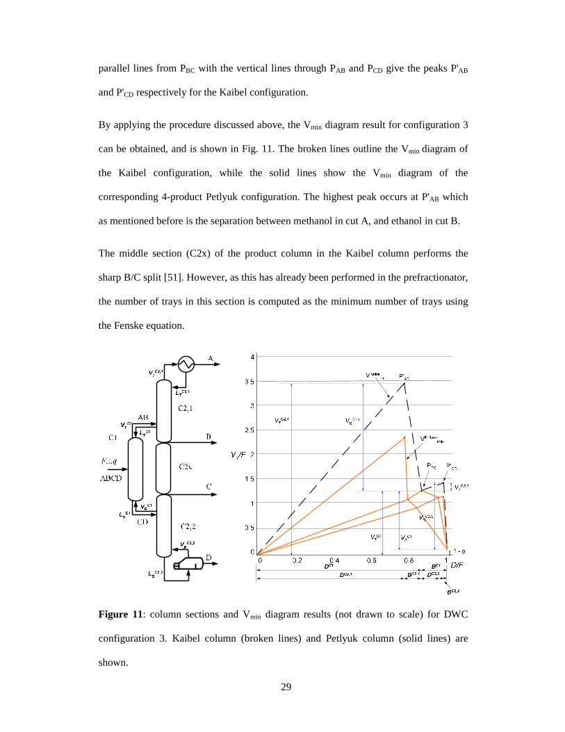
By applying the procedure discussed above, the Vmin diagram result for configuration 3

can be obtained, and is shown in Fig. 11. The broken lines outline the Vmin diagram of

the Kaibel configuration, while the solid lines show the Vmin diagram of the

corresponding 4-product Petlyuk configuration. The highest peak occurs at P'AB which

as mentioned before is the separation between methanol in cut A, and ethanol in cut B.

The middle section (C2x) of the product column in the Kaibel column performs the

sharp B/C split [51]. However, as this has already been performed in the prefractionator,

the number of trays in this section is computed as the minimum number of trays using

the Fenske equation.

Figure 11: column sections and Vmin diagram results (not drawn to scale) for DWC

configuration 3. Kaibel column (broken lines) and Petlyuk column (solid lines) are

shown.

30

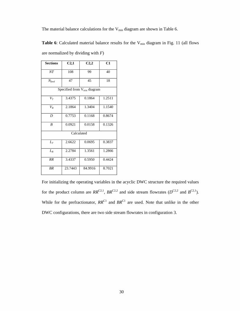
The material balance calculations for the Vmin diagram are shown in Table 6.

Table 6: Calculated material balance results for the Vmin diagram in Fig. 11 (all flows

are normalized by dividing with F)

Sections C2,1 C2,2 C1

NT 108 99 40

Nfeed 47 45 18

Specified from Vmin diagram

VT 3.4375 0.1864 1.2511

VB 2.1864 1.3404 1.1540

D 0.7753 0.1168 0.8674

B 0.0921 0.0158 0.1326

Calculated

LT 2.6622 0.0695 0.3837

LB 2.2784 1.3561 1.2866

RR 3.4337 0.5950 0.4424

BR 23.7443 84.9916 8.7021

For initializing the operating variables in the acyclic DWC structure the required values

for the product column are RRC2,1, BRC2,2 and side stream flowrates (DC2,2 and BC2,1).

While for the prefractionator, RRC1 and BRC1 are used. Note that unlike in the other

DWC configurations, there are two side stream flowrates in configuration 3.

31

4.2 Optimization results (optimal structures)

4.2.1 Base case

Figure 12: Base case showing the optimal structure of the columns, and condenser and

reboiler duties

The base case is set up using the data shown in Table 1 with the results of its optimal

structure shown in Fig. 12. For the base case each column is optimized individually.

Each column is divided into 2 column sections with the number of trays in each column

section as decision variables (NI and NII). Furthermore, the bounds of each decision

variable were kept between 4 and 80 for the optimization. In addition, it should be noted

that the PSO was re-run using a variety of different sets of initial conditions for the

swarm, but the algorithm always converged on the same optimum result. The results

show that the first column which recovers methanol and lighter components (cut A) in

the distillate is the largest, both in terms of number of trays, and condenser and reboiler

duties. The higher energy requirement in this column can be explained by the larger

flowrate into the first column, the large amount of methanol in the feed (68.3 mol %),

and the close boiling point between methanol and ethanol (HK component in cut B). All

these make recovering > 99.3 % mole recovery of methanol in the distillate difficult and

32

more energy intensive in comparison to the other columns. Note also that though this

column is tall, at approximately 91.3 m, it is below 110 m (about 175 trays) which is the

maximum height recommended for distillation columns [41].

4.2.2 DWC configurations 1 and 2

Figure 13: Model for DWC configuration 1 showing (a) simulation structure, with PSO

variables and bounds (b) optimal structure of the equivalent DWC design with the

condenser and reboiler duties, liquid split ratio (rL) and vapor split ratio (rV)

In DWC configuration 1, the first column is a conventional methanol recovery column

with specification and results as discussed for column 1 of the base case in section 4.2.1.

The output of that column, with feed properties as shown in Table 3, is subsequently fed

into the 3-product DWC. In comparison to a conventional column, there are additional

operating and structural variables for minimizing the TAC of the DWC. This is because

of the presence of a side stream in the DWC, as well as the interconnection between the

prefractionator and product columns of the DWC. In the process simulator, five

operating variables need to be specified for simulating the acyclic DWC structure.

33

These are the RR, BR and side stream flowrate of the product column, as well as the RR

and BR of the prefractionator. The initialization of these variables is done using the

results of the Vmin method shown in section 4.1.1. In the process simulator setup the

operating variables of the product column are varied to meet the specifications of the

product streams (RR for B, side stream flowrate for C, and BR for D). This leaves the

two operating variables of the prefractionator as degrees of freedom which can be

varied to minimize the reboiler duty. However, in this study we simplify the process

simulator setup and leave the values of RR and BR of the prefractionator at their Vmin

result values. To optimize the 3-product DWC structure, five independent discrete

variables are used as shown in Fig. 13 (a) with their respective bounds. Variables NI -

NIV relate to the number of trays in the sections of the product column, while variable

NV relates to the feed location at the prefractionator. In reality the prefractionator of the

DWC is in fact located in the product column; thus a simplifying assumption is that the

number of trays in the prefractionator is equivalent to the number of trays in the

corresponding part of the product column i.e. the summation of variables NII and NIII.

This assumption means that an over-separation will be performed on one side of the

dividing wall. However, the approach is still very reasonable as the most difficult

separations determine the height of the DWC. The resulting optimal structure after

optimization is shown in Fig. 13 (b).

In DWC configuration 2, the DWC column is placed before a conventional column for

butanol recovery. Apart from the difference in feed properties into the DWC column, its

process simulation setup and optimization is similar to that of the DWC column in

configuration 1. The structure setup and optimal structure for configuration 2 are shown

in Fig. 14.

34

Figure 14: Model for DWC configuration 2 showing (a) simulation structure, with PSO

variables and bounds (b) optimal structure of the equivalent DWC design with the

condenser and reboiler duties, liquid split ratio (rL) and vapor split ratio (rV)

4.2.3 DWC configuration 3

In configuration 3, a 4-product DWC based on a Kaibel configuration is used. The

additional product in this configuration means that in comparison to the 3-product DWC

an extra operating variable needs to be specified for the operation of the column, and an

extra discrete variable for optimizing the structure. The extra operating variable is the

side stream flowrate of the additional side product, while an additional discrete variable

is added to represent the column section between the two side products. Similar to the 3-

product DWC configurations, the prefractionator operating variables are kept constant

at their Vmin values while the product column's operating variables are varied to meet

product specifications during the process simulation. The number of trays in the

prefractionator is given as the summation of variables NII - NIV, with the assumption that

the number of trays in the prefractionator is equal to the number of trays in the

35

equivalent sections of the product column also being maintained. Fig. 15 shows the

structure setup and optimal structure.

Figure 15: DWC configuration 3 showing (a) simulation structure, with PSO variables

and bounds (b) optimal structure of the equivalent DWC design with the condenser and

reboiler duties, liquid split ratio (rL) and vapor split ratio (rV)

4.3 Optimization results (economics)

The economic results of all the cases studied are shown in Table 7. As can been seen,

configurations 1 to 3 all have better economic results than the base case, with the least

amount of savings experienced for configuration 1. This is because the methanol

recovery column, which is the column with the most significant cost in the base case,

also contributes to configuration 1. In configuration 3, the advantages of implementing

all product recoveries in one DWC column is quite clear, as savings in TAC of up to 28

% in comparison to the base case are obtained. These savings are mainly as a result of

huge savings (31 %) in operating costs obtained in this configuration. These results

highlight the big potential that DWCs have in replacing conventional columns in the

36

separation section of the thermochemical biobutanol process. It is also conceivable that

similar savings might be obtainable for other biofuel applications.

Table 7: Operating cost, capital cost and TAC results for all cases studied

Base case

Op. Cost (k$/yr) Cap. Cost (k$) TAC (k$/yr)

Methanol recovery column 2,075 1,550 2,484

Ethanol/propanol recovery column 513 681 693

Butanol recovery column 126 165 170

Total 2,714 2,396 3,346

Configuration 1

Op. Cost (k$/yr) Cap. Cost (k$) TAC (k$/yr)

Methanol recovery column 2,075 1,550 2,484

3-product DWC 579 755 778

Total 2,654 2,305 3,262

Savings with respect to base case 2.2% 3.8% 2.5%

Configuration 2

Op. Cost (k$/yr) Cap. Cost (k$) TAC (k$/yr)

3-product DWC 2,098 2,053 2,640

Butanol recovery column 126 165 170

Total 2,225 2,218 2,810

Savings with respect to base case 18.0% 7.4% 16.0%

Configuration 3

Op. Cost (k$/yr) Cap. Cost (k$) TAC (k$/yr)

4-product DWC 1,878 2,033 2,414

Savings with respect to base case 30.8% 15.2% 27.9%

4.4 Sensitivity analysis on best configuration (configuration 3)

As has been seen from the results obtained in the prior section, the best configuration

for the separation is configuration 3, the 4-product DWC. In this section, a sensitivity

37

analysis on the results of configuration 3 is carried out on some of the key economic

assumptions made in this work such as the depreciation time, interest rate, utility price

and cost of the sieve trays in the dividing wall section, to see the effect of these

parameters on the TAC and the column structure (number of trays). These results are

shown graphically in Fig. 16, with the TAC trends shown with solid lines, and the

number of trays trends shown with the hashed trend lines. The relationship between the

TAC and number of trays versus the interest rate is shown in Fig. 16 (a). Increasing the

interest rate increases the TAC, as the cost of borrowing capital becomes higher, while

the opposite occurs when the interest rate is reduced. However, the number of trays in

the column remains the same. In Fig. 16 (b), a plot of the change in TAC and number of

trays with respect to annualization time is shown. As can be seen, an increase in

annualization time from the base case results in a decrease in TAC and vice versa with a

decrease in the annualization time. The increased annualization time means that capital

cost repayments are spread over a longer time period, thus reducing the annualization

factor and the contribution of the capital cost to the TAC, the opposite occurs when the

annualization time is reduced. Note that the exponential relationship between the TAC

and annualization time is a result of the exponential relationship between the

annualization factor and annualization time as can be seen in equation (7).

The change in the number of trays follows a trend which is opposite to the change in

TAC. This is because with an increase in annualization time, the cost of borrowing

capital becomes cheaper thus favoring columns with more trays. In Fig. 16 (c), the TAC

and optimal number of trays are plotted against the utility price. The values on the x-

axis of this figure are percentage changes in utility (steam and cooling water) price from

the base case values, with 100 % representing the base case. The plot shows that a linear

direct relationship exists between the TAC and utility price as expected based on the

38

equations discussed in section 3.4. The change in the number of trays with respect to the

utility price also follows a linear trend. This is because as the operating cost is

increased, taller columns are favored and vice versa when the operating cost is reduced.

Finally, the TAC and number of trays are plotted against the cost factor assumed for the

sieve trays in the dividing wall section of the DWC. As is seen in Fig. 16 (d), the

relationship between the TAC and sieve tray factor is linear. Increasing the tray factor

means that the sieve trays are more expensive for the DWCs thus causing an increase in

the TAC, and vice versa when the tray factor is reduced. However, the change in the

number of trays with respect to the tray factor is linear but opposite to the TAC. This is

because smaller columns are favored when the cost of the sieve trays, and thus capital

cost are increased. It should be noted that noise in the data is due to suboptimal results

generated by the PSO, since the number of iterations was restricted to 100 for each case.

Figure 16: Sensitivity analysis on results of best configuration (configuration 3)

140

145

150

155

160

165

170

175

180

2,300

2,350

2,400

2,450

2,500

2,550

2,600

0 5 10 15 20 25

Nu

mb

er o

f tr

ays

TA

C (

k$/

yr)

Interest rate (%)

140

145

150

155

160

165

170

175

180

2,000

2,100

2,200

2,300

2,400

2,500

2,600

2,700

2,800

0 5 10 15 20 25

Nu

mb

er o

f tr

ays

TA

C (

k$/

yr)

Annualization time (year)

140

145

150

155

160

165

170

175

180

1,000

1,500

2,000

2,500

3,000

3,500

4,000

4,500

0 50 100 150 200 250

Nu

mb

er o

f tr

ays

TA

C (

k$/

yr)

Utility price (% of base case)

140

145

150

155

160

165

170

175

180

2,300

2,350

2,400

2,450

2,500

2,550

2,600

2,650

1 1.5 2 2.5 3 3.5

Nu

mb

er o

f tr

ays

TA

C (

k$/

yr)

Tray cost factor (-)

39

5. Conclusion

This work has looked at the design of DWC configurations for application to the

separation section of a thermochemical biobutanol process. A general methodology

based on the use of shortcut methods for column initialization, and a two-tier simulation

- optimization strategy was discussed and used for design of the DWCs. The results

show that all the DWC configurations provide cost savings in comparison to a base case

configuration of three conventional columns in direct sequence. Furthermore, the 4-

product DWC provides the most savings, with up to 31 % savings in operating costs,

and 28 % savings in TAC. Note that these savings are reasonable and in line with the

general savings reported for DWCs in other cases. Therefore, it can be concluded that

the implementation of DWC technology in a thermochemical biobutanol process can

lead to cost savings and thus improvements in the overall economics of the process. In

future work the authors intend to carry out a full system study to quantify how the use

of DWC configurations impact on the production cost of biobutanol from the

thermochemical route.

6. Acknowledgement

This work was funded by an Ontario Research Fund – Research Excellence Grant (ORF

RE-05-072)

Nomenclature

F feed flowrate (kmol/hr)

z composition

q feed quality, liquid fraction

VT vapor flow in the top section of the column (kmol/hr)

D distillate (kmol/hr)

Nmin minimum number of trays

40

liquid flow at the top of the column (kmol/hr)

liquid flow at the bottom of the column (kmol/hr)

vapor flow at the bottom of the column (kmol/hr)

bottoms flow rate (kmol/hr)

s tray spacing (m)

H column height (m)

NT number of trays

f annualization factor

i fractional interest rate per year

n annualization period in years (yr)

RR reflux ratios

BR boilup ratios

Dia column diameter (m)

Nj number of trays in the jth section of the product column

Nfeed tray number of feed location

Qreb reboiler duty (MW)

Qcond condenser duty (MW)

Treb reboiler temperature ()

Tcond condenser temperature ()

rL liquid split ratio

rV vapor split ratio

References

[1] International Energy Agency, World Energy Outlook 2013, 2013. http://www.worldenergyoutlook.org/media/weowebsite/2013/WEO2013_Ch06_Renewables.pdf.

[2] Ö. Yildirim, A. A. Kiss, E.Y. Kenig, Dividing wall columns in chemical process industry: A review on current activities, Sep. Purif. Technol. 80 (2011) 403–417.

[3] R. Agrawal, Z.T. Fidkowski, Are Thermally Coupled Distillation Columns Always Thermodynamically More Efficient for Ternary Distillations ?, 5885 (1998) 3444–3454.

41

[4] R.R. Rewagad, A. A. Kiss, Dynamic optimization of a dividing-wall column using model predictive control, Chem. Eng. Sci. 68 (2012) 132–142.

[5] N. Asprion, G. Kaibel, Dividing wall columns: Fundamentals and recent advances, Chem. Eng. Process. Process Intensif. 49 (2010) 139–146.

[6] A. A. Kiss, R.M. Ignat, Innovative single step bioethanol dehydration in an extractive dividing-wall column, Sep. Purif. Technol. 98 (2012) 290–297.

[7] A. A. Kiss, Distillation technology - still young and full of breakthrough opportunities, J. Chem. Technol. Biotechnol. 89 (2014) 479–498.

[8] L.Y. Sun, X.W. Chang, C.X. Qi, Q.S. Li, Implementation of Ethanol Dehydration Using Dividing-Wall Heterogeneous Azeotropic Distillation Column, Sep. Sci. Technol. 46 (2011) 1365–1375.

[9] I. Dejanović, L. Matijašević, Ž. Olujić, Dividing wall column—A breakthrough towards sustainable distilling, Chem. Eng. Process. Process Intensif. 49 (2010) 559–580.

[10] A. A. Kiss, C.S. Bildea, A control perspective on process intensification in dividing-wall columns, Chem. Eng. Process. Process Intensif. 50 (2011) 281–292.

[11] H. Ling, W.L. Luyben, New Control Structure for Divided-Wall Columns, Ind. Eng. Chem. Res. 48 (2009) 6034–6049.

[12] D. Dwivedi, J.P. Strandberg, I.J. Halvorsen, S. Skogestad, Steady state and dynamic operation of four-product dividing-wall (Kaibel) columns: Experimental verification, Ind. Eng. Chem. Res. 51 (2012) 15696–15706.

[13] M. Kumar, K. Gayen, Developments in biobutanol production: New insights, Appl. Energy. 88 (2011) 1999–2012.

[14] A. Ranjan, V.S. Moholkar, Biobutanol: science, engineering, and economics, Int. J. Energy Resour. 36 (2012) 277–323.

[15] C. Okoli, T.A. Adams II, Design and economic analysis of a thermochemical lignocellulosic biomass-to-butanol process, Ind. Eng. Chem. Res. 53 (2014) 11427–11441.

[16] A. A. Kiss, Novel applications of dividing-wall column technology to biofuel production processes, J. Chem. Technol. Biotechnol. 88 (2013) 1387–1404.

[17] A. A. Kiss, R.M. Ignat, Enhanced methanol recovery and glycerol separation in biodiesel production - DWC makes it happen, Appl. Energy. 99 (2012) 146–153.

[18] M. Ghadrdan, I.J. Halvorsen, S. Skogestad, Optimal operation of Kaibel distillation columns, Chem. Eng. Res. Des. 89 (2011) 1382–1391.

42

[19] I. Dejanović, L. Matijašević, I.J. Halvorsen, S. Skogestad, H. Jansen, B. Kaibel, et al., Designing four-product dividing wall columns for separation of a multicomponent aromatics mixture, Chem. Eng. Res. Des. 89 (2011) 1155–1167.

[20] I.J. Halvorsen, S. Skogestad, Minimum Energy Consumption in Multicomponent Distillation. 1. Vmin Diagram for a Two-Product Column, Ind. Eng. Chem. Res. 42 (2003) 596–604.

[21] I.J. Halvorsen, S. Skogestad, Minimum Energy Consumption in Multicomponent Distillation. 2. Three-Product Petlyuk Arrangements, Ind. Eng. Chem. Res. 42 (2003) 605–615.

[22] I.J. Halvorsen, S. Skogestad, Minimum Energy Consumption in Multicomponent Distillation. 3. More Than Three Products and Generalized Petlyuk Arrangements, Ind. Eng. Chem. Res. 42 (2003) 616–629.

[23] A. A. Kiss, R.M. Ignat, S.J. Flores Landaeta, A.B. De Haan, Intensified process for aromatics separation powered by Kaibel and dividing-wall columns, Chem. Eng. Process. Process Intensif. 67 (2013) 39–48.

[24] L. Sun, X. Bi, Shortcut method for the design of reactive dividing wall column, Ind. Eng. Chem. Res. 53 (2014) 2340–2347.

[25] J. Javaloyes-Antón, R. Ruiz-Femenia, J. A. Caballero, Rigorous Design of Complex Distillation Columns Using Process Simulators and the Particle Swarm Optimization Algorithm, Ind. Eng. Chem. Res. 52 (2013) 15621–15634.

[26] J. Leboreiro, J. Acevedo, Processes synthesis and design of distillation sequences using modular simulators: a genetic algorithm framework, Comput. Chem. Eng. 28 (2004) 1223–1236.

[27] M. Gendreau, J.-Y. Potvin, Handbook of Metaheuristics Vol. 2, Springer, New York, 2010.

[28] A. Kaveh, Advances in Metaheuristic Algorithms for Optimal Design of Structures, Springer, New York, 2014.

[29] A. Pascall, T. A. Adams II, Semicontinuous separation of dimethyl ether (DME) produced from biomass, Can. J. Chem. Eng. 91 (2013) 1001–1021.

[30] M.A. Navarro, J. Javaloyes, J.A. Caballero, I.E. Grossmann, Strategies for the robust simulation of thermally coupled distillation sequences, Comput. Chem. Eng. 36 (2012) 149–159.

[31] ASTM Standard D7862-15, Standard Specification for Butanol for Blending with Gasoline for Use as Automotive Spark-Ignition Engine Fuel, (2015). doi:10.1520/D7862-15.

[32] K. Ramakrishnan, P.L. Sabarethinam, Pet. Chem. Ind. Dev. 11 (1977) 19–22.

43

[33] J.M. Resa, C. Gonzalez, J.M. Goenaga, M. Iglesias, Density, Refractive Index, and Speed of Sound at 298.15 K and Vapor−Liquid Equilibria at 101.3 kPa for Binary Mixtures of Ethyl Acetate + 1-Pentanol and Ethanol + 2-Methyl-1-propanol, J. Chem. Eng. Data. 49 (2004) 804–808.

[34] A.S. Mozzhukhin, V.A. Mitropol’skaya, L.A. Serafimov, A.I. Torubarov, T.S. Rudakovskaya, Zhurnal Fiz. Khimii. 41 (1967) 227.

[35] K. Kojima, K. Tochigi, H. Seki, K. Watase, Determination of vapor-liquid equilibrium from boiling point curve, Kagaku Kogaku Ronbunshu. 32 (1968) 149–153.

[36] K. Kurihara, M. Nakamichi, K. Kojima, Isobaric vapor-liquid equilibria for methanol + ethanol + water and the three constituent binary systems, J. Chem. Eng. Data. 38 (1993) 446 – 449.

[37] K. Ochi, K. Kojima, Vapor-liquid equilibrium for ternary systems consisting of alcohols and water, Kagaku Kogaku Ronbunshu. 33 (1969) 352.

[38] W.D. Seider, J.D. Seader, D.R. Lewin, Product & Process Design Principles: Synthesis, Analysis and Evaluation, 3rd ed., John Wiley & Sons, Hoboken, New Jersey, 2009.

[39] A.K. Modi, A.W. Westerberg, Distillation column sequencing using marginal price, Ind. Eng. Chem. Res. 31 (1992) 839 – 848.

[40] G. Kaibel, Distillation columns with vertical partitions, Chem. Eng. Technol. 10 (1987) 92–98.

[41] Ž. Olujić, M. Jödecke, A. Shilkin, G. Schuch, B. Kaibel, Equipment improvement trends in distillation, Chem. Eng. Process. Process Intensif. 48 (2009) 1089–1104.

[42] T.A. Adams II, W.D. Seider, Practical optimization of complex chemical processes with tight constraints, Comput. Chem. Eng. 32 (2008) 2099–2112.

[43] S. Boubaker, M. Djemai, N. Manamanni, F. M’Sahli, Active modes and switching instants identification for linear switched systems based on Discrete Particle Swarm Optimization, Appl. Soft Comput. 14 (2014) 482–488.

[44] P.C. Wankat, Separations in chemical engineering: equilibrium staged separations., Elsevier, New York, 1988.

[45] U.E.I.A. EIA, Henry Hub Gulf Coast Natural Gas Spot Price, (2012). http://www.eia.gov/dnav/ng/hist/rngwhhdW.htm.

[46] I.E.S.O. IESO, Hourly Ontario Energy Price, (2012). http://www.ieso.ca/Pages/Power-Data/default.aspx.

44

[47] G. Towler, R. Sinnott, Chemical engineering design: principles, practice and economics of plant and process design, 2nd Edition, Butterworth-Heinemann, Massachusetts, 2012.

[48] G.P. Rangaiah, E.L. Ooi, R. Premkumar, A Simplified Procedure for Quick Design of Dividing-Wall Columns for Industrial Applications, Chem. Prod. Process Model. 4 (2009) 1–42.

[49] R. Smith, Chemical process design and integration, John Wiley & Sons, Chichester, 2005.

[50] I.J. Halvorsen, S. Skogestad, Minimum Energy for the four-product Kaibel-column, in: AIChE annual meeting, 2006.

[51] M. Ghadrdan, I.J. Halvorsen, S. Skogestad, A Shortcut Design for Kaibel Columns Based on Minimum Energy Diagrams, in: E.N. Pistikopoulos, M.C. Georgiadis, A.C. Kokossis (Eds.), 21st Eur. Symp. Comput. Aided Process Eng. ESCAPE 21, Elsevier B.V., Porto Carras, Greece, 2011: pp. 356 – 360.