ARTICLE IN PRESS - d1rkab7tlqy5f1.cloudfront.net faculteit/Afdelingen... · UNCORRECTED PROOF...

DTD 5 ARTICLE IN PRESS

1

2

3

4

5

6

7

8

9

10

11

12

13

14

15

16

17

18

19

20

21

22

23

24

25

26

27

28

29

30

31

32

33

34

35

36

37

38

39

40

41

42

43

44

45

46

47

48

49

50

51

52

53

54

55

56

57

58

59

60

61

62

63

64

65

66

67

68

69

70

71

72

73

74

75

76

77

78

79

80

81

82

83

ECTED PROOF

Testing for nonlinearity of streamflow processes

at different timescales

Wen Wanga,b,*, J.K. Vrijlingb, Pieter H.A.J.M. Van Gelderb, Jun Mac

aFaculty of Water Resources and Environment, Hohai University, Nanjing 210098, ChinabFaculty of Civil Engineering and Geosciences, Section of Hydraulic Engineering, Delft University of Technology. P.O. Box 5048, 2600 GA

Delft, NetherlandscYellow River Conservancy Commission, Hydrology Bureau, Zhengzhou 450004, China

Accepted 8 February 2005

Abstract

Streamflow processes are commonly accepted as nonlinear. However, it is not clear what kind of nonlinearity is acting

underlying the streamflow processes and how strong the nonlinearity is for the streamflow processes at different timescales.

Streamflow data of four rivers are investigated in order to study the character and type of nonlinearity that are present in the

streamflow dynamics. The analysis focuses on four characteristic time scales (i.e. one year, one month, 1/3 month and one day),

with BDS test to detect for the existence of general nonlinearity and the correlation exponent analysis method to test for the

existence of a special case of nonlinearity, i.e. low dimensional chaos. At the same time, the power of the BDS test as well as the

importance of removing seasonality from data for testing nonlinearity are discussed. It is found that there are stronger and more

complicated nonlinear mechanisms acting at small timescales than at larger timescales. As the timescale increases from a day to

a year, the nonlinearity weakens, and the nonlinearity of some 1/3-monthly and monthly streamflow series may be dominated

by the effects of seasonal variance. While nonlinear behaviour seemed to be present with different intensity at the various time

scales, the dynamics would not seem to be associable to the presence of low dimensional chaos.

q 2005 Published by Elsevier B.V.

Keywords: Nonlinearity; BDS test; Stationarity; KPSS test; Chaos detection; Correlation dimension

84

85

86

87

88

89

90

ORR1. Introduction

A major concern in many scientific disciplines is

whether a given process should be modeled as linear

or as nonlinear. It is currently well accepted that many

natural systems are nonlinear with feedbacks over

UNC0022-1694/$ - see front matter q 2005 Published by Elsevier B.V.

doi:10.1016/j.jhydrol.2005.02.045

* Corresponding author. Tel.: C86 25 378 7530.

E-mail address: [email protected] (W. Wang).

HYDROL 14830—15/6/2005—00:45—SHYLAJA—151845—XML MODEL 3 – p

91

92

93

94

many space and timescales. However, certain aspects

of these systems may be less nonlinear than others and

the nature of nonlinearity may not be always clear

(Tsonis, 2001). As an example of natural systems,

streamflow processes are also commonly perceived as

nonlinear. They could be governed by various

nonlinear mechanisms acting on different temporal

and spatial scales. Investigations on nonlinearity and

applications of nonlinear models to streamflow series

have received much attention in the past two decades

Journal of Hydrology xx (xxxx) 1–22

www.elsevier.com/locate/jhydrol

p. 1–22

95

96

http://www.elsevier.com/locate/jhydrol

C

H

W. Wang et al. / Journal of Hydrology xx (xxxx) 1–222


97

98

99

100

101

102

103

104

105

106

107

108

109

110

111

112

113

114

115

116

117

118

119

120

121

122

123

124

125

126

127

128

129

130

131

132

133

134

135

136

137

138

139

140

141

142

143

144

145

146

147

148

149

150

151

152

153

154

155

156

157

158

159

160

161

162

163

164

165

166

167

168

169

170

171

172

173

174

175

176

177

178

179

180

181

182

183

184

185

186

187

188

189

190

191

192

UNCORRE

(e.g. Rogers, 1980, 1982; Rogers and Zia, 1982; Rao

and Yu, 1990; Chen and Rao, 2003). Rogers (1980,

1982) and Rogers and Zia (1982) developed a

heuristic method to quantify the degree of nonlinear-

ity of drainage basins by using rainfall-runoff data.

Rao and Yu (1990) used Hinich bispectrum test

(1982) to investigate the linearity and nongaussian

characteristics of annual streamflow and daily rainfall

and temperature series. They detected nonlinearity in

daily meteorological series, but not in annual stream-

flow series. Chen and Rao (2003) investigated

nonlinearity in monthly hydrologic time series with

the Hinich test. The results indicate that all of the

stationary segments of standardized monthly tem-

perature and precipitation series are either Gaussian or

linear, and some of the standardized monthly stream-

flow are nonlinear.

As a special case of nonlinearity, chaos is widely

concerned in the last two decades, and chaotic

mechanism of streamflows has been increasingly

gaining interests of the hydrology community (e.g.

Wilcox et al., 1991; Jayawardena and Lai, 1994;

Porporato and Ridolfi, 1996; Sivakumar et al., 1999;

Elshorbagy et al., 2002). Most of the research in

literature confirms the presence of chaos in the

hydrologic time series. Nonetheless, the existence of

low-dimensional chaos has been a topic in wide

dispute (e.g. Ghilardi and Rosso, 1990; Koutsoyiannis

and Pachakis, 1996; Pasternack, 1999; Schertzer

et al., 2002).

In spite of all the advances in the research on the

nonlinear characteristics of streamflow processes,

further investigation is still desirable, because on

one hand, there is no common knowledge about what

type of nonlinearity exists in the streamflow process,

and on the other hand, it is not clear how the character

and intensity of nonlinearity of streamflow processes

changes as the timescale changes. More insights into

the nature of nonlinearity would allow one to decide

whether a specific process should be modeled with a

linear or a nonlinear model.

It is hard to explore different types of nonlinearity

one by one which may possibly act underlying

streamflow processes. We here want to investigate

the existence of general nonlinearity in the streamflow

process from a univariate time series data based

quantitative point of view. However, there is no direct

general measure of nonlinearity so far, therefore,

YDROL 14830—15/6/2005—00:45—SHYLAJA—151845—XML MODEL 3 – pp

TED PROOF

testing for nonlinearity basically is carried out by

testing for linearity as an alternative. There are a wide

variety of methods available presently to test for

linearity or nonlinearity, which may be divided into

two categories: portmanteau tests, which test for

departure from linear models without specifying

alternative models, and the tests designed for some

specific alternatives. Patterson and Ashley (2000)

applied 6 portmanteau test methods to 8 artificially

generated nonlinear series of different types, and

found that the BDS test is the best and clearly stands

out in terms of overall power against a variety of

alternatives. The power of BDS test and some

nonparametric tests have also recently been compared

and applied to residual analysis of fitted models for

monthly rainfalls by Kim et al. (2003), and the results

also indicate the effectiveness of BDS test. As for the

test for the existence of chaos, there are many methods

available nowdays, among which the correlation

exponent method (e.g. Grassberger and Procaccia,

1983a), the Lyapunov exponent method (e.g. Wolf

et al., 1985), the Kolmogorov entropy method (e.g.

Grassberger and Procaccia, 1983b), the nonlinear

prediction method (e.g. Farmer and Sidorowich, 1987;

Sugihara and May, 1990), and the surrogate data

method (e.g. Theiler et al., 1992; Schreiber and

Schmitz, 1996) are commonly used.

In this paper, two issues are addressed. First, in

Section 4, streamflow series of different timescales,

namely, one year, one month, 1/3-month and one day,

of four streamflow processes in different climate

regions are studied to investigate the existence and

intensity of general nonlinearity with the BDS test.

Second, in Section 6, correlation exponent method

will be applied to test for the presence of chaos in the

streamflow series of four rivers. Correlation exponent

method is the most important method for detecting

chaos, and it is used by almost all the researchers for

detecting chaos in hydrological processes (e.g.

Jayawardena and Lai, 1994; Porporato and Ridolfi,

1997; Pasternack, 1999; Bordignon and Lisi, 2000;

Elshorbagy et al., 2002). The analysis based on the

correlation exponent method is done with software

TISEAN (Hegger et al., 1999). In addition, in Section

2, the datasets which are used for this study are

described, followed by an introduction to the BDS test

in Section 3, and the power analysis of BDS test in

. 1–22

W. Wang et al. / Journal of Hydrology xx (xxxx) 1–22 3


193

194

195

196

197

198

199

200

201

202

203

204

205

206

207

208

209

210

211

212

213

214

215

216

217

218

219

220

221

222

223

224

225

226

227

228

229

230

231

232

233

234

235

236

237

238

239

240

241

242

Section 5. Finally, the paper ends with a discussion

and conclusion in Sections 7 and 8, respectively.

C

O

243

244

245

246

247

248

249

250

251

252

253

254

255

256

257

258

259

260

261

262

263

264

265

266

267

268

269

270

271

272

273

274

275

276

277

278

279

280

281

282

283

284

285

286

287

288

UNCORRE

2. Data used

Streamflow series of four rivers, i.e. the Yellow

River in China, the Rhine River in Europe, the

Umpqua River and the Ocmulgee River in the United

States, are analyzed in this study.

The first streamflow process is the streamflow of

the Yellow River at Tangnaihai. The gauging station

Tangnaihai has a 133,650 km2 drainage basin in the

northeastern Tibet Plateau, including an permanently

snow-covered area of 192 km2. The length of main

channel in this watershed is over 1500 km. Most of

the watershed is 3000–6000 m above sea level.

Snowmelt water composes about 5% of total runoff.

Because the watershed is partly permanently snow-

covered and sparsely populated, without any large-

scale hydraulic works, the streamflow process is

fairly pristine.

The second one is the streamflow of the Rhine

River at Lobith, the Netherlands. The Rhine is one of

Europe’s best-known and most important rivers. Its

length is 1320 km. The catchment area is about

170,000 km2. The gauging station Lobith is located

at the lower reaches of the Rhine, near German-

Dutch border. Due to favorable distribution of

precipitation over the catchment area, the Rhine

has a rather equal discharge. The data are provided

by the Global Runoff Data Centre (GRDC) in

Germany (http://grdc.bafg.de/).

The third one is the streamflow of the Umpqua

River near Elkton, Oregon in the United states. The

drainage area is 9535 km2. The datum of the gauge is

90.42 feet above sea level. The record started from

October 1905. Regulation by powerplants on North

Umpqua River ordinarily does not affect discharge at

this station. There are diversions for irrigation

upstream from the station.

The fourth one is the streamflow of the upper

Ocumlgee River at Macon, Georgia. The station

Macon has a drainage area of 5799 km2. Its gauge

datum is 269.80 feet above sea level. The headwaters

of the Ocmulgee River begin in the highly urbanized

Atlanta metropolitan area, and downstream its

watershed is dominated by agriculture and forested


OF

areas. The daily discharge data of both the Umpqua

River and the Ocmulgee River are available from the

USGS (United States Geological Survey) website

http://water.usgs.gov/waterwatch/.

Monthly series are obtained from daily data by

taking average of daily discharges in every month.

For the 1/3-monthly series, the 1st and 2rd 1/3-month

streamflows are the averages of the first and the

second 10-days’ daily discharges, and the 3rd 1/3-

month discharge is the average of the last 8–11 days’

daily discharges of a month depending on the length

of the month. All the daily data series used here start

from January 1, and end on December 31. The

statistical characteristics of the streamflow series at

different timescales are summarized in Table 1. The

plots of mean daily discharges and standard

deviations of these streamflow series are shown in

Fig. 1.

TED PR3. BDS test

The BDS test (Brock et al., 1996) is a nonpara-

metric method for testing for serial independence and

nonlinear structure in a time series based on the

correlation integral of the series. As stated by the

authors, the BDS statistic has its origins in the work

on deterministic nonlinear dynamics and chaos

theory, it is not only useful in detecting deterministic

chaos, but also serves as a residual diagnostic tool that

can be used to test the goodness-of-fit of an estimated

model. The null hypothesis is that the time series

sample comes from an independent identically

distributed (i.i.d.) process. The alternative hypothesis

is not specified. In this section, the theoretical aspects

of BDS test are presented.

Embed a scalar time series {xt} of length N into a

m-dimensional space, and generate a new series {Xt},

XtZ(xt, xtKt,.,xtK(mK1)t), Xt2Rm. Then, calculate

the correlation integral Cm,M (r) given by (Grassberger

and Procaccia, 1983a):

Cm;MðrÞZM

2

!K1 X1%i!j%M

HðrK jjXi KXjjjÞ; (1)

where MZN-(mK1) t is the number of embedded

points inm-dimensional space; r the radius of a sphere

centered on Xi; H(u) is the Heaviside function, with

p. 1–22

http://grdc.bafg.de/

http://water.usgs.gov/waterwatch/

OF

Table 1

Statistical characteristics of streamflow series

River (station) Period of

record

Timescale Mean (m3/s) Standard devi-

ation (m3/s)

Skewness

coefficient

Kurtosis coef-

ficient

ACF(1)

Yellow

(Tangnaihai)

1956–2000 Daily 646 559 1.864 5.034 0.994

1/3-monthly 643 549 1.770 4.472 0.884

Monthly 643 521 1.516 2.789 0.703

Annual 646 166 0.882 K0.076 0.301

Rhine (Lobith) 1901–1996 Daily 2217 1147 2.121 7.162 0.985

1/3-monthly 2219 1072 1.755 4.602 0.713

Monthly 2219 928 1.230 2.143 0.544

Annual 2217 471 K0.135 K0.567 0.140

Umpqua

(Elkton)

1906–2001 Daily 210 306 5.193 49.344 0.864

1/3-monthly 211 247 2.614 11.126 0.627

Monthly 211 209 1.625 3.325 0.621

Annual 210 57.8 0.401 K0.193 0.233

Ocmulgee

(Macon)

1929–2001 Daily 76.1 106.2 6.711 76.506 0.857

1/3-monthly 76.4 80.9 3.508 19.331 0.500

Monthly 76.3 63.8 1.903 4.653 0.537

Annual 76.1 25.9 0.556 0.441 0.254

H



289

290

291

292

293

294

295

296

297

298

299

300

301

302

303

304

305

306

307

308

309

310

311

312

313

314

315

316

317

318

319

320

321

322

323

324

325

326

327

328

329

330

331

332

333

334

335

336

337

338

339

340

341

342

343

344

345

346

347

348

349

350

351

352

353

354

355

356

357

358

359

360

361

H(u)Z1 for uO0, and H(u)Z0 for u%0; k(k denotes

the sup-norm.

Cm,M (r) counts up the number of points in the

m-dimensional space that lie within a hypercube

of radius r. Brock et al. (1996) exploit the asymptotic

normality of Cm,M (r) under the null hypothesis

UNCORREC0

300

600

900

1200

1500

1800

0 60 120 180 240 300 360

Day

Dis

char

ge (

m3 /

s)

0

5000

10000

15000

20000

25000

30000

0 60 120 180 240 300 360

Day

Dis

char

ge (

ft3 /s)

MeanSD

Yellow River at Tangnaihai

Mean

SD

Umpqua River near Elkton

(a) (b

(c) (d

Fig. 1. Variation in daily mean and standar


PRO

that {xt} is an i.i.d. process to obtain a test

statistic which asymptotically converges to a unit

normal.

If the series is generated by a strictly stationary

stochastic process that is absolutely regular, then the

limit CmðrÞZ limN/NCm;MðrÞ exists. In this case the

TED

0 60 120 180 240 300 360

Day

0

2000

4000

6000

8000

10000

12000

Dis

char

ge (

ft3 /s)

500

0

10001500

20002500

30003500

0 60 120 180 240 300 360

Day

Dis

char

ge (

m3 /

s)

Mean

SD

Rhine River at Lobith

Mean

SD

Ocmulgee River at Macon

)

)

d deviation of streamflow processes.

. 1–22

362

363

364

365

366

367

368

369

370

371

372

373

374

375

376

377

378

379

380

381

382

383

384

C



385

386

387

388

389

390

391

392

393

394

395

396

397

398

399

400

401

402

403

404

405

406

407

408

409

410

411

412

413

414

415

416

417

418

419

420

421

422

423

424

425

426

427

428

429

430

431

432

433

434

435

436

437

438

439

440

441

442

443

444

445

446

447

448

449

450

451

452

453

454

455

456

457

458

459

460

461

462

463

464

465

466

467

468

469

470

471

472

473

474

475

476

477

478

479

480

UNCORRE

limit is

CmðrÞZ

ððHðrK jjXKYjjÞdFmðXÞdFmðYÞ; (2)

where Fm denote the distribution function of

embedded time series {Xt}.

When the process is independent, and since

HðrK jjXiKYjjjÞZQm

kZ1 HðrK jXi;kKYj;kjÞ, Eq. (2)

implies that CmðrÞZCm1 ðrÞ. Also CmðrÞKCm

1 ðrÞ has

asymptotic normal distribution, with zero mean and

variance given by

1

4s2m;MðrÞZmðmK2ÞC2mK2ðKKC2ÞCKm KC2m

C2XmK1

jZ1

½C2jðKmKj KC2mK2jÞKmC2mK2ðKKC2Þ�:

(3)

The constants C and K in Eq. (3) can be estimated

by

CMðrÞZ1

M2

XMiZ1

XMjZ1

HðrK jjXi KXjjjÞ;

and

KMðrÞZ1

M3

XMiZ1

XMjZ1

XMkZ1

HðrK jjXi KXjjjÞ

HðrK jjXj KXkjjÞ:

Under the null hypothesis that {xt} is an i.i.d.

process, the BDS statistic for mO1 is defined as

BDSm;MðrÞZffiffiffiffiffiM

p CmðrÞKCm1 ðrÞ

sm;MðrÞ: (4)

It asymptotically converges to a unit normal as

M/N. This convergence requires large samples for

values of embedding dimension mmuch larger than 2,

so m is usually restricted to the range from 2 to 5.

Brock et al. (1991) recommend that r is set to between

half and three halves the standard deviation s of the

data. We find that if r is set as half s, there would be

too few or even no nearest neighbors for many points

in the embedded m-dimensional space whenm is large

(e.g.mZ5), especially for series of short size (e.g. less

than 100); on the other hand, when r is set as three

halves s, there would be too many nearest neighbors

for many points in the embedded m-dimensional


space when m is small (e.g. mZ2). Such kind of

‘shortage’ of neighbors or ‘excess’ of neighbors will

probably bias the calculation of Cm,M(r). Therefore,

we only consider r equal to the standard deviation of

the data in this study.

TED PROOF

4. Test results for streamflow processes

4.1. Stationarity test

Because usually linearity/nonlinearity tests (e.g.

BDS test) assume the series of interest is stationary, it

is necessary to test the stationarity before taking

nonlinearity test. The stationarity test is carried out

with two methods, one is augmented Dickey-Fuller

(ADF) unit root test proposed by Dickey and Fuller

(1979), which tests for the presence of unit root in the

series (difference stationarity); another is KPSS test

proposed by Kwiatkowski et al. (1992), which tests

for the stationarity around a deterministic trend (trend

stationarity) and the stationarity around a fixed level

(level stationarity). To achieve stationarity, if a

process is difference stationary with unit roots, the

appropriate treatment is to difference the series; if not

level stationary but trend stationary, which indicates

that there is a deterministic trend, then we should

remove the trend component from the series.

Because on one hand both ADF test and KPSS test

are based on linear regression, which has normal

distribution assumption; on the other hand, logarith-

mization can convert exponential trend possibly

present in the data into linear trend, therefore, it is

common to take logs of the data before applying ADF

test and KPSS test (e.g. Gimeno et al., 1999). In this

study, the streamflow data are also logarithmized

before applying stationarity tests. An important

practical issue for the implementation of the ADF

test as well as the KPSS test is the specification of the

lag length l. Following Schwert (1989); Kwiatkowski

et al. (1992), the number of lag length in this study is

chosen as lZ int½xðT=100Þ1=4�, with xZ4, 12.

The stationarity test results are given in Table 2.

All the monthly and 1/3-monthly series appear to be

stationary, since we cannot accept the unit root

hypothesis with ADF test at 1% significance level

and cannot reject the trend stationarity hypothesis and

level stationarity hypothesis with KPSS test at

p. 1–22

ECTED PROOF

Table 2

Stationarity test results for streamflow series

Station Series KPSS level stationary test KPSS trend stationary test ADF unit roots test

Lag Results p-value Lag Results p-value Lag Results p-value

Yellow

(Tangnaihai)

Daily 14 0.366 O0.05 14 0.366 !0.01 14 K4.887 3.00!10K4

42 0.138 O0.1 42 0.138 O0.05 42 K4.887 3.00!10K4

1/3-

montly

8 0.078 O0.1 8 0.078 O0.1 8 K6.243 3.53!10K7

24 0.113 O0.1 24 0.113 O0.1 24 K6.243 3.53!10K7

Monthly 6 0.084 O0.1 6 0.084 O0.1 6 K7.295 1.16!10K9

18 0.115 O0.1 18 0.115 O0.1 18 K7.295 1.16!10K9

Annual 3 0.165 O0.1 3 0.161 O0.01 3 K4.689 2.53!10K3

9 0.142 O0.1 9 0.139 O0.05 9 K4.689 2.53!10K3

Rhine

(Lobith)

Daily 17 0.413 O0.05 17 0.394 !0.01 17 K12.86 2.44!10K32

51 0.186 O0.1 51 0.178 O0.01 51 K12.86 2.44!10K32

1/3-

montly

9 0.119 O0.1 9 0.114 O0.1 9 K19.93 4.95!10K65

29 0.076 O0.1 29 0.073 O0.1 29 K19.93 4.95!10K65

Monthly 7 0.088 O0.1 7 0.081 O0.1 7 K16.24 1.30!10K43

22 0.064 O0.1 22 0.059 O0.1 22 K16.24 1.30!10K43

Annual 3 0.075 O0.1 3 0.053 O0.1 3 K8.57 3.23!10K10

11 0.112 O0.1 11 0.082 O0.1 11 K8.57 3.23!10K10

Umpqua

(Elkton)

Daily 17 0.254 O0.1 17 0.242 !0.01 17 K18.67 5.76!10K62

51 0.101 O0.1 51 0.096 O0.1 51 K18.67 5.76!10K62

1/3-

montly

9 0.061 O0.1 9 0.059 O0.1 9 K15.17 2.88!10K42

29 0.136 O0.1 29 0.133 O0.1 29 K15.17 2.88!10K42

Monthly 7 0.079 O0.1 7 0.08 O0.1 7 K12.39 5.92!10K28

22 0.133 O0.1 22 0.132 O0.05 22 K12.39 5.92!10K28

Annual 3 0.101 O0.1 3 0.101 O0.1 3 K7.124 1.11!10K07

11 0.094 O0.1 11 0.093 O0.1 11 K7.124 1.11!10K07

Ocmulgee

(Macon)

Daily 16 0.543 O0.01 16 0.408 !0.01 16 K30.23 1.40!10K115

48 0.228 O0.1 48 0.171 O0.01 48 K30.23 1.40!10K115

1/3-

montly

9 0.128 O0.1 9 0.1 O0.1 9 K18.46 4.33!10K57

27 0.121 O0.1 27 0.095 O0.1 27 K18.46 4.33!10K57

Monthly 6 0.097 O0.1 6 0.086 O0.1 6 K12.81 7.03!10K29

20 0.081 O0.1 20 0.072 O0.1 20 K12.81 7.03!10K29

Annual 3 0.056 O0.1 3 0.055 O0.1 3 K6.311 6.27!10K6

11 0.085 O0.1 11 0.083 O0.1 11 K6.311 6.27!10K6

Note: Critical value of KPSS distribution for level stationarity hypothesis: 10% w0.347; 5% w0.463; 1% w0.739; Critical value of KPSS

distribution for trend stationarity hypothesis: 10% w0.119; 5% w0.146; 1% w0.216.

H



481

482

483

484

485

486

487

488

489

490

491

492

493

494

495

496

497

498

499

500

501

502

503

504

505

506

507

508

509

510

511

512

513

514

515

516

517

518

519

520

521

522

523

524

525

526

527

528

529

530

531

532

533

534

535

536

537

538

539

540

541

542

543

544

545

546

547

548

549

550

551

552

553

554

555

556

557

558

559

560

561

562

563

564

565

566

567

568

569

570

571

572

573

574

575

576

UNCORRthe 10% level. All the series pass KPSS level

stationary test, which means that all the series are

stationary around a fixed level and there is no

significant change in mean. But some daily series

cannot pass trend stationary test when the lag is small.

This is probably partly because of the influence of

serial dependence at short-lags, and partly because the

trend fitted to the daily series in trend stationary test

could be over-affected by some outlier data, thus

make the whole series not stationary around such a

biased trend. However, for large lags, all the daily

series pass the trend-stationary test, although some


pass at comparatively low significance level (O0.01).

Therefore, all the series are basically stationary, and

no differencing or de-trending operation is needed.

4.2. Nonlinearity test

BDS test needs the extraction of linear structure

from the original series by the use of an estimated

linear filter. Therefore, the first step for the test is

fitting linear models to the streamflow series.

Because streamflow processes (except annual

series) usually exhibit strong seasonality, to analysis

. 1–22

C

Table 3

Order of AR models fitted to streamflow series

Timescale Yellow Rhine Umpqua Ocmulgee

Raw Log Log-DS Raw Log Log-DS Raw Log Log-DS Raw Log Log-DS

Daily – 41 38 – 39 40 – 45 36 – 43 44

1/3-

monthly

– 32 6 – 6 16 – 35 7 – 33 8

Monthly – 23 4 – 29 4 – 27 5 – 29 3

Annual 1 – – 6 – – 2 – – 1 – –



577

578

579

580

581

582

583

584

585

586

587

588

589

590

591

592

593

594

595

596

597

598

599

600

601

602

603

604

605

606

607

608

609

610

611

612

613

614

615

616

617

618

619

620

621

622

623

624

625

626

627

628

629

630

631

632

633

634

635

636

637

638

639

640

641

642

643

644

645

646

647

648

649

650

651

652

653

654

655

656

657

658

659

660

661

662

663

664

665

666

667

668

669

670

671

672

UNCORRE

the role of the seasonality played in nonlinearity test,

the streamflow series are pre-processed in two ways,

logarithmization and deseasonalization. Correspond-

ingly, the pre-processed series are referred to as Log

series and Log-DS series respectively. The Log-DS

series is obtained with two steps. Firstly, logarithmize

the flow series. Then deseasonalize them by subtract-

ing the seasonal (e.g. daily or monthly) mean values

and dividing by the seasonal standard deviations of

the logarithmized series. To alleviate the stochastic

fluctuations of the daily means and standard devi-

ations, we smooth them with first 8 Fourier harmonics

before using them for standardization. Annual series

is analyzed without any transformation. All series are

pre-whitened with AR models. The autoregressive

orders of the AR models are selected according to

AIC, shown in Table 3. Residuals are obtained from

these models, then the BDS test is applied to the

residual series.

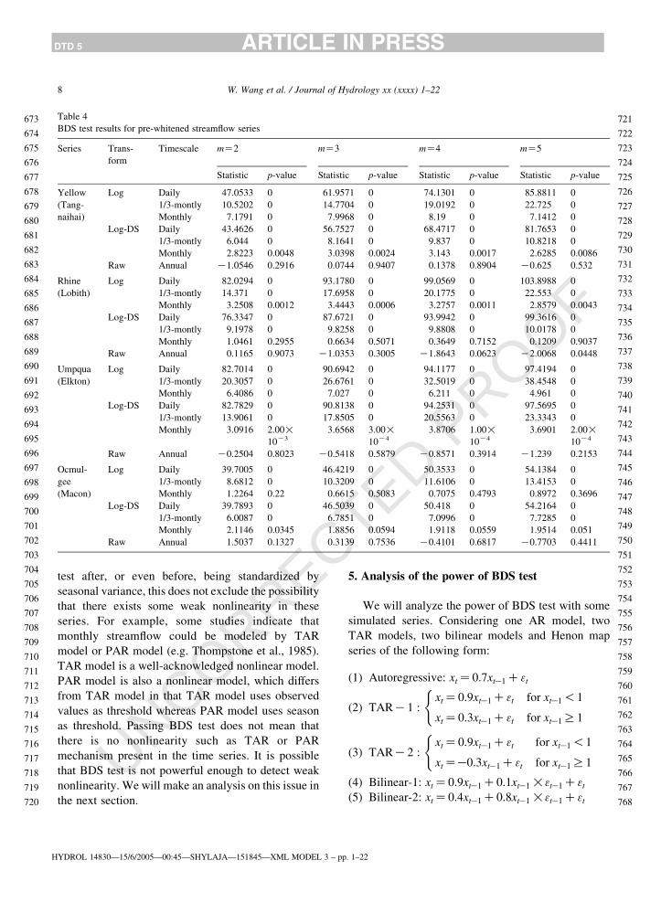
Test results are shown in Table 4. It is shown in

Table 4 that all the annual series pass the BDS test,

indicating that annual flow series are linear. This

result is in agreement with that of Rao and Yue

(1990). Among the monthly series, Log series of

Ocmulgee and Log-DS series of Rhine pass the BDS

test, while Log-DS series of Ocmulgee narrowly pass

the test at significance level 0.05. But all the other

series cannot pass BDS test at 0.01 significance level.

It is noted that, with the increase of the timescale, the

nonlinearity decreases. Among the flow series at four

characteristic time scales, the strongest nonlinearity

exists in daily series and the least nonlinearity exists

in annual series. Except for the daily and monthly

streamflow series of Ocmulgee, and daily flow of

Umpqua, there is a general feature that the test

statistics of Log-DS series are smaller than those of


TED PROOF

the Log series, which implies that deseasonalization

may more or less alleviates the nonlinearity.

With a close inspection of the residual series, we

find that although the residuals are serially uncorre-

lated, there is seasonality in the variance of the

residual series. Therefore, it is worthwhile to have a

look at the residuals after removing such kind of

season-dependent variance. Table 5 shows the BDS

test results for the residual series after being

standardized with seasonal variance.

Comparing Tables 4 and 5, we can find that, the

BDS test statistics of all the series are generally

smaller than those of the series before standardization.

Especially, 1/3-montly and monthly Log-DS series of

the Yellow River, and the monthly Log series of the

Rhine River, which are nonlinear before standardiz-

ation, pass the BDS test at 0.05 significance level after

standardization. Therefore, the seasonal variation in

variance in the residuals is probably a dominant

source of nonlinearity in the 1/3-montly and monthly

Log-DS series of the Yellow River, and the monthly

Log series of the Rhine River. But all the daily series,

most 1/3-monthly series and some monthly series still

exhibit nonlinearity even after standardization. That

indicates that the seasonal variance composes only a

small, even negligible, fraction of the nonlinearity

underlying these processes, especially daily stream-

flow processes.

The above analysis indicates that there are stronger

and more complicated nonlinearity mechanisms

acting at small timescales than at large timescales.

As the timescale increases, the nonlinearity weakens,

and the effects of seasonal variance dominate the

nonlinearity of some 1/3-monthly and monthly

streamflow series.

Although most monthly flow series and some

1/3-monthly series are diagnosed as linear with BDS

p. 1–22

CTED PROOF

Table 4

BDS test results for pre-whitened streamflow series

Series Trans-

form

Timescale mZ2 mZ3 mZ4 mZ5

Statistic p-value Statistic p-value Statistic p-value Statistic p-value

Yellow

(Tang-

naihai)

Log Daily 47.0533 0 61.9571 0 74.1301 0 85.8811 0

1/3-montly 10.5202 0 14.7704 0 19.0192 0 22.725 0

Monthly 7.1791 0 7.9968 0 8.19 0 7.1412 0

Log-DS Daily 43.4626 0 56.7527 0 68.4717 0 81.7653 0

1/3-montly 6.044 0 8.1641 0 9.837 0 10.8218 0

Monthly 2.8223 0.0048 3.0398 0.0024 3.143 0.0017 2.6285 0.0086

Raw Annual K1.0546 0.2916 0.0744 0.9407 0.1378 0.8904 K0.625 0.532

Rhine

(Lobith)

Log Daily 82.0294 0 93.1780 0 99.0569 0 103.8988 0

1/3-montly 14.371 0 17.6958 0 20.1775 0 22.553 0

Monthly 3.2508 0.0012 3.4443 0.0006 3.2757 0.0011 2.8579 0.0043

Log-DS Daily 76.3347 0 87.6721 0 93.9942 0 99.3616 0

1/3-montly 9.1978 0 9.8258 0 9.8808 0 10.0178 0

Monthly 1.0461 0.2955 0.6634 0.5071 0.3649 0.7152 0.1209 0.9037

Raw Annual 0.1165 0.9073 K1.0353 0.3005 K1.8643 0.0623 K2.0068 0.0448

Umpqua

(Elkton)

Log Daily 82.7014 0 90.6942 0 94.1177 0 97.4194 0

1/3-montly 20.3057 0 26.6761 0 32.5019 0 38.4548 0

Monthly 6.4086 0 7.027 0 6.211 0 4.961 0

Log-DS Daily 82.7829 0 90.8138 0 94.2531 0 97.5695 0

1/3-montly 13.9061 0 17.8505 0 20.5563 0 23.3343 0

Monthly 3.0916 2.00!10K3

3.6568 3.00!10K4

3.8706 1.00!10K4

3.6901 2.00!10K4

Raw Annual K0.2504 0.8023 K0.5418 0.5879 K0.8571 0.3914 K1.239 0.2153

Ocmul-

gee

(Macon)

Log Daily 39.7005 0 46.4219 0 50.3533 0 54.1384 0

1/3-montly 8.6812 0 10.3209 0 11.6106 0 13.4153 0

Monthly 1.2264 0.22 0.6615 0.5083 0.7075 0.4793 0.8972 0.3696

Log-DS Daily 39.7893 0 46.5039 0 50.418 0 54.2164 0

1/3-montly 6.0087 0 6.7851 0 7.0996 0 7.7285 0

Monthly 2.1146 0.0345 1.8856 0.0594 1.9118 0.0559 1.9514 0.051

Raw Annual 1.5037 0.1327 0.3139 0.7536 K0.4101 0.6817 K0.7703 0.4411

H



673

674

675

676

677

678

679

680

681

682

683

684

685

686

687

688

689

690

691

692

693

694

695

696

697

698

699

700

701

702

703

704

705

706

707

708

709

710

711

712

713

714

715

716

717

718

719

720

721

722

723

724

725

726

727

728

729

730

731

732

733

734

735

736

737

738

739

740

741

742

743

744

745

746

747

748

749

750

751

752

753

754

755

756

757

758

759

760

761

762

763

764

765

766

767

768

UNCORREtest after, or even before, being standardized by

seasonal variance, this does not exclude the possibility

that there exists some weak nonlinearity in these

series. For example, some studies indicate that

monthly streamflow could be modeled by TAR

model or PAR model (e.g. Thompstone et al., 1985).

TAR model is a well-acknowledged nonlinear model.

PAR model is also a nonlinear model, which differs

from TAR model in that TAR model uses observed

values as threshold whereas PAR model uses season

as threshold. Passing BDS test does not mean that

there is no nonlinearity such as TAR or PAR

mechanism present in the time series. It is possible

that BDS test is not powerful enough to detect weak

nonlinearity. We will make an analysis on this issue in

the next section.


5. Analysis of the power of BDS test

We will analyze the power of BDS test with some

simulated series. Considering one AR model, two

TAR models, two bilinear models and Henon map

series of the following form:

(1) Autoregressive: xtZ0:7xtK1C3t

(2) TARK1 :xtZ0:9xtK1C3t for xtK1!1

xtZ0:3xtK1C3t for xtK1R1

(

(3) TARK2 :xtZ0:9xtK1C3t for xtK1!1

xtZK0:3xtK1C3t for xtK1R1

(

(4) Bilinear-1: xtZ0:9xtK1C0:1xtK1!3tK1C3t(5) Bilinear-2: xtZ0:4xtK1C0:8xtK1!3tK1C3t

. 1–22

UNCORRECTED PROOF

Table 5

BDS test results for standardized pre-whitened streamflow series

Series Transform Timescale mZ2 mZ3 mZ4 mZ5

Statistic p-value Statistic p-value Statistic p-value Statistic p-value

Yellow

(Tang-

naihai)

Log Daily 36.5463 0 46.8049 0 55.9885 0 63.2352 0

1/3-montly 3.2901 1.00!10K3 3.9963 1.00!10K4 4.8369 0 5.0091 0

Monthly 3.3106 9.00!10K4 3.6546 3.00!10K4 3.8527 1.00!10K4 3.6088 3.00!10K4

Log-DS Daily 39.4409 0 46.3156 0 50.7325 0 54.8716 0

1/3-montly 1.572 0.116 1.9548 0.0506 1.8772 0.0605 1.3839 0.1664

Monthly 0.2841 0.7763 0.0009 0.9993 0.2121 0.8321 0.33 0.7414

Rhine

(Lobith)

Log Daily 75.4414 0 87.4872 0 94.4997 0 100.7701 0

1/3-montly 6.2161 0 6.0256 0 5.6061 0 5.2266 0

Monthly 0.0469 0.9626 K0.4685 0.6394 K0.6538 0.5132 K0.6077 0.5434

Log-DS Daily 76.0273 0 88.0100 0 94.9955 0 101.1316 0

1/3-montly 6.9859 0 6.5541 0 5.7396 0 5.0427 0

Monthly 0.3254 0.7449 K0.1996 0.8418 K0.3752 0.7075 K0.563 0.5735

Umpqua

(Elkton)

Log Daily 79.2755 0 87.0849 0 90.5519 0 93.9577 0

1/3-montly 11.4493 0 12.9663 0 13.1782 0 13.3861 0

Monthly 3.3133 9.00!10K4 3.8847 1.00!10K4 4.0829 0 3.9246 1.00!10K4

Log-DS Daily 79.4946 0 87.334 0 90.8304 0 94.294 0

1/3-montly 10.8964 0 12.6817 0 13.1041 0 13.604 0

Monthly 2.2041 0.0275 2.7437 0.0061 3.0048 0.0027 3.0525 0.0023

Ocmulgee

(Macon)

Log Daily 39.2541 0 45.9753 0 49.8505 0 53.5797 0

1/3-montly 8.1499 0 9.351 0 10.4597 0 12.1685 0

Monthly 1.1009 0.271 0.4957 0.6201 0.5591 0.5761 0.8345 0.404

Log-DS Daily 39.339 0 46.0532 0 49.9094 0 53.6486 0

1/3-montly 5.495 0 5.8351 0 5.99 0 6.6117 0

Monthly 1.839 0.0659 1.6546 0.098 1.6696 0.095 1.6642 0.0961

HYDROL14830—

15/6/2005—

00:46—

SHYLAJA

—151845—

XMLMODEL3–pp.1–22

W.Wanget

al./JournalofHydrologyxx

(xxxx)1–22

9

DTD

5ARTICLEIN

PRESS

769

770

771

772

773

774

775

776

777

778

779

780

781

782

783

784

785

786

787

788

789

790

791

792

793

794

795

796

797

798

799

800

801

802

803

804

805

806

807

808

809

810

811

812

813

814

815

816

817

818

819

820

821

822

823

824

825

826

827

828

829

830

831

832

833

834

835

836

837

838

839

840

841

842

843

844

845

846

847

848

849

850

851

852

853

854

855

856

857

858

859

860

861

862

863

864

C

H



865

866

867

868

869

870

871

872

873

874

875

876

877

878

879

880

881

882

883

884

885

886

887

888

889

890

891

892

893

894

895

896

897

898

899

900

901

902

903

904

905

906

907

908

909

910

911

912

913

914

915

916

917

918

919

920

921

922

923

924

925

926

927

928

929

930

931

932

933

934

935

936

937

938

939

940

941

942

943

944

945

(6) Henon map

series :xtC1Z1Kax2t Cbyt; aZ1:4; bZ0:3

ytC1Zxt

�

In all the above models, {xt} (or {yt}) is time

series, and {3t} is independent standard normal error.

Obviously, among the above models, model TAR-1

and Bilinear-1 have weak nonlinearity while model

TAR-2 and Bilinear-2 have stronger nonlinearity,

because TAR-2 has a larger parameter difference and

Bilinear-2 has a more significant bilinear item.

Henon map series is a typical chaotic series

(Henon, 1976). For model (1) to (5), 1000

simulations are generated, and each simulation has

500 points. For Henon series, one simulation with

500000 points is generated (referred to as clean-

Henon in Table 6). Then the Henon series is divided

into 1000 segments, and each segment has 500

points. To evaluate the influence of noise on BDS

test, noise is added to the simulated Henon series

(referred to as noise-Henon in Table 6). The noise is

normally distributed with zero mean, and its standard

deviation is 5% of the standard deviation of the

Henon series.

Then we use BDS test to detect the presence of

nonlinearity in the simulated series. All the series

are pre-whitened with AR models. The test results

are shown in Table 6. It is shown that the

hypothesis of linearity for Henon series (pure or

with noise) are firmly rejected, which indicates that

BDS test is very powerful for detecting such kind

of strong nonlinearity. In most cases, BDS test

correctly rejects the hypothesis that TAR-2 and

UNCORRETable 6

Rates of accepting linearity with BDS test based on 1000 replications at s

Series mZ2 mZ3

p-value Accepted p-value Accep

AR(1) 0.4832 926 0.4836 925

TAR-1 0.3612 831 0.3713 838

TAR-2 0.0024 212 0.0037 272

Bilinear-1 0.1780 703 0.1964 714

Bilinear-2 6.729!10K40 0 5.977!10K46 0

Clean-Henon 7.235!10K50 0 3.266!10K84 0

Noise-Henon 3.611!10K49 0 5.315!10K82 0

Note: p-value in the table is the median value for each group of 1000 rep


TED PROOF

Bilinear-2 processes are linear, but wrongly accepts

TAR-1 and Blinear-1 processes as linear. That

means that although BDS test is considered very

powerful for testing nonlinearity, but not powerful

enough for detecting weak nonlinearity in TAR-1

and Bilinear-1, whereas such kinds of weak

nonlinearity probably present in the streamflow

series, because it is impossible that streamflow

processes are driven by the mechanism like TAR-2,

which switches between dramatically different

regimes.

Therefore, BDS test results tell us that there is

strong nonlinearity present in daily streamflow

series as well as most 1/3-monthly series, even

after taking away the effects of seasonal variance,

but there is no strong nonlinearity presents in most

monthly streamflow series and some 1/3-monthly

series after removing the effects of seasonal

variance. However, we cannot say there is no

nonlinearity present in those 1/3-monthly and

monthly streamflow series even if they pass BDS

test, because BDS test is not powerful enough for

detecting weak nonlinearity. In addition, comparing

the BDS test results for chaotic Henon series with

those for streamflow series, while it is not clear

whether most 1/3-monthly series and all the daily

series have chaotic properties, it seems that all

monthly series may not be chaotic because the

BDS test p-values for monthly flow series are far

much higher than those for chaotic Henon series.

We would further detect the existence of chaos

with correlation exponent method in the next

section.

ignificance level 0.05

mZ4 mZ5

ted p-value Accepted p-value Accepted

0.4840 928 0.4621 933

0.3798 840 0.4034 843

0.0088 326 0.0140 373

0.2383 735 0.2644 763

3.624!10K47 0 3.617!10K47 0

3.496!10K115 0 2.252!10K142 0

5.829!10K112 0 5.922!10K138 0

lications.

. 1–22

946

947

948

949

950

951

952

953

954

955

956

957

958

959

960

UNCORRECTED PROOF

0 1000 2000 3000 4000 5000

x (t )

0 1000 2000 3000 4000 5000

x (t )0 1000 2000 3000 4000 5000

x (t )

0 1000 2000 3000 4000 5000

x (t )

0

1000

2000

3000

4000

5000

x (t

+1)

0

1000

2000

3000

4000

5000

x (t

+10

)

0

1000

2000

3000

4000

5000

x (t

+7)

0

1000

2000

3000

4000

5000

x (t

+20

)

(a) (b)

(c) (d)

Fig. 3. xt-xtCt state-space maps of daily streamflow series of the Yellow River at Tangnaihai with (a) tZ1; (b) tZ7; (c) tZ10; (d) tZ20.

ACF

MI

0 6 12 18 24 30 36

Lag

– 0.8– 0.6– 0.4– 0.2

00.20.40.60.8

1

AC

F /

MI

(c)

–1

– 0.5

0

0.5

1

1.5

0 120 240 360 480 600

Lag

AC

F /

MI

–1

– 0.5

0.5

0

1

0 12 24 36 48 60 72

Lag

AC

F /

MI

(a) (b)

Fig. 2. ACF and MI of (a) daily, (b) 1/3-monthly and (c) monthly river flow of the Yellow River.

HYDROL 14830—15/6/2005—00:46—SHYLAJA—151845—XML MODEL 3 – pp. 1–22



961

962

963

964

965

966

967

968

969

970

971

972

973

974

975

976

977

978

979

980

981

982

983

984

985

986

987

988

989

990

991

992

993

994

995

996

997

998

999

1000

1001

1002

1003

1004

1005

1006

1007

1008

1009

1010

1011

1012

1013

1014

1015

1016

1017

1018

1019

1020

1021

1022

1023

1024

1025

1026

1027

1028

1029

1030

1031

1032

1033

1034

1035

1036

1037

1038

1039

1040

1041

1042

1043

1044

1045

1046

1047

1048

1049

1050

1051

1052

1053

1054

1055

1056

C

H



1057

1058

1059

1060

1061

1062

1063

1064

1065

1066

1067

1068

1069

1070

1071

1072

1073

1074

1075

1076

1077

1078

1079

1080

1081

1082

1083

1084

1085

1086

1087

1088

1089

1090

1091

1092

1093

1094

1095

1096

1097

1098

1099

1100

1101

1102

1103

1104

1105

1106

1107

1108

1109

1110

1111

1112

1113

1114

1115

1116

1117

1118

1119

1120

1121

1122

1123

1124

1125

1126

1127

1128

1129

1130

1131

1132

1133

1134

1135

1136

1137

1138

1139

1140

1141

1142
RRE
6. Test for chaos in streamflow processes with

correlation exponent method

When testing for general nonlinearity, it is common

to filter the data to remove linear correlations

(prewhitening) (e.g. Brock et al., 1996), because linear

autocorrelation can give rise to spurious results in

algorithms for estimating nonlinear invariants, such as

correlation dimension and Lyapunov exponents. But it

has been observed that in numerical practice prewhiten-

ing may severely impairs the underlying deterministic

nonlinear structure of low-dimensional chaotic time

series (e.g. Theiler and Eubank, 1993; Sauer and Yorke,

1993). Therefore, mostly chaos analyses are based on

original series, and the same in our analysis.

Correlation exponent method is most frequently

employed to investigate the existence of chaos. The

basis of this method is multi-dimension state space

reconstruction. The most commonly used method for

reconstructing the state space is the time-delay

coordinate method proposed by Packard et al.

(1980); Takens (1981). In the time delay coordinate

method, a scalar time series {x1, x2,.,xN} is

converted to state vectors XtZ(xt,xt-t,.,xt-(mK1)t)

after determining two state space parameters: the

embedding dimension m and delay time t. To check

whether chaos exists, the correlation exponent values

are calculated against the corresponding embedding

dimension values. If the correlation exponent leads to

a finite value as embedding dimension increasing,

then the process under investigation is thought of as

being dominated by deterministic dynamics. Other-

wise, the process is considered as stochastic.

To calculate the correlation exponent, the delay

time t should be determined first. Therefore, the

selection of delay time is discussed first in the

following section, followed by the estimation of

correlation dimension.
1143
1144

1145

1146

1147

1148

1149

1150

1151

1152

UNCO6.1. Selection of delay time

The delay time T is commonly selected by using

the autocorrelation function (ACF) method where

ACF first attains zeros or below a small value (e.g. 0.2

or 0.1), or the mutual information (MI) method

(Fraser and Swinney, 1986) where the MI first attains

a minimum. We first take the streamflow of the


TED PROOF

Yellow River at Tangnaihai as an example to analyze

the choice of T.We calculate ACF andMI of daily, 1/3-monthly and

monthlyflowseriesof theYellowRiver, shown inFig. 2.

Because of strong seasonality, ACF first attains zeros at

the lag time of about 1/4 period, namely, 91, 9 and 3 for

daily, 1/3-monthly andmonthly series respectively. The

MI method gives similar estimates for T to the ACF

method, about approximately 1/4 annual period.

In practice, the estimate of t is usually application

and author dependent nonetheless in practice. For

instance, for daily flow series, some authors take the

delay time as 1 day (Porporato andRidolfi, 1997), 2 days

(Jayawardena and Lai, 1994), 7 days (Islam and

Sivakumar, 2002), 10 days (Elshorbagy et al., 2002),

20 days (Wilcox et al., 1991) and 146 days (Pasternack,

1999). These differences may arise from different ACF

structure. To compare the influence of differentT on the

reconstruction of state space, we can plot xtwxtCt state-

space maps for the streamflow series with different T.The best T value should make the state space best

unfolded. For the streamflow series of theYellowRiver,

the xtwxtCt state-spacemapswith smallTvalues (i.e. 1,

7, 10, and 20) are displayed in Fig. 3, and the 2- and

3-dimensional xtwxtCt state-space maps with t taken

as 1/4 of the annual period are displayed in Fig. 4.

Obviously, especially clearly in the 3-D maps, state

spaces for daily, 1/3-monthly and monthly streamflow

series are best unfolded when delay time TZ91, 9, 3

respectively.

We therefore select TZ91, 9, 3 for estimating

correlation dimension for the streamflow series of the

Yellow River. Similar results are obtained for the

sreamflow processes of the Umpqua River and the

Ocmulgee River (to save space, the plots are not

displayed here). But for the Rhine River, the seasonality

is not that obvious. The ACF and MI of daily, 1/3-

monthly and monthly flow series of the Rhine River are

shown in Fig. 5. If we determine the delay time

according to the lags where ACF attains 0 or MI attains

its minimum for the Rhine River, the lags would be

about 200 days which seems to be too large, which

would possibly make the successive elements of the

state vectors in the embedded multi-dimensional state

space almost independent. Thereforewe select the delay

time equal to the lags before ACF attains 0.1, namely,

TZ92, 9, 3 for daily, 1/3-monthly and monthly

streamflow series, respectively.

. 1–22

ORRECTED PROOF

0 1000 2000 3000 4000 5000

x (t)

0 1000 2000 3000 4000 5000

x (t)

0 1000 1500500 2000 2500 3000 3500

x (t)

0

1000

2000

3000

4000

5000

x (t

+91

)

0

1000

2000

3000

4000

5000

x (t

+9)

0

1000

2000

3000

x (t

+3)

x (t)

x (t+91)

x (t+182)

x (t+18)

x (t+9)

x (t)

x (t)

x (t+3)

x (t+6)

(d)

(a) (b)

(c) (d)

(e) (f)

Fig. 4. 2-D and 3-D state space maps of (a), (b) daily; (c), (d) 1/3-monthly; and (e), (f) monthly streamflow of the Yellow River at Tangnaihai

with delay time tZ91, 9 and 3.



1153

1154

1155

1156

1157

1158

1159

1160

1161

1162

1163

1164

1165

1166

1167

1168

1169

1170

1171

1172

1173

1174

1175

1176

1177

1178

1179

1180

1181

1182

1183

1184

1185

1186

1187

1188

1189

1190

1191

1192

1193

1194

1195

1196

1197

1198

1199

1200

1201

1202

1203

1204

1205

1206

1207

1208

1209

1210

1211

1212

1213

1214

1215

1216

1217

1218

1219

1220

1221

1222

1223

1224

1225

1226

1227

1228

1229

1230

1231

1232

1233

1234

1235

1236

1237

1238

1239

1240

1241

1242

1243

1244

1245

1246

1247

1248

UNC6.2. Estimation of correlation dimension

The most commonly used algorithm for computing

correlation dimension is Grassberger - Procaccia

algorithm (Grassberger and Procaccia, 1983a), modi-

fied by Theiler (1986). For a m-dimension phase-

space, the modified correlation integral C(r) is defined


by (Theiler, 1986)

CðrÞZ2

ðMC1KwÞðMKwÞ

XMiZ1

XMKi

jZiCwC1

Hðr

K jjXi KXjjjÞ; (5)

p. 1–22

UNCORRECTED PROOF

AC

F /

MI

ACF

MI

– 0.5

0

0.5

1

1.5

AC

F /

MI

– 0.2

0

0.8

0.6

0.4

0.2

0 120 240 360 480 600

Lag

0 12 24 36 48 60 72

Lag

AC

F /

MI

– 0.2

0.8

0.6

0.4

0.2

0

0 6 12 18 24 30 36

Lag

(a) (b)

(c)

Fig. 5. ACF and MI of (a) daily, (b) 1/3-monthly and (c) monthly river flow of the Rhine River.

–15

–12

– 9

– 6

– 3

02 3 4 5 6 7 8 9

6 7 8 9 10 11 12 65 7 8 9 10 11

3 4 5 6 7 8 9

lnr

lnr lnr

Yellow River Rhine River

lnC

(r )

–15

–12

– 9

– 6

– 3

0

LnC

(r )

–15

–12

– 9

– 6

– 3

0

lnC

(r )

–15

–12

– 9

– 6

– 3

0

lnC

(r )

Umpqua River Ocmulgee River

(a) (b)

(c) (d)

lnr

Fig. 6. ln C(r) versus ln r plot for daily streamflow processes.




1249

1250

1251

1252

1253

1254

1255

1256

1257

1258

1259

1260

1261

1262

1263

1264

1265

1266

1267

1268

1269

1270

1271

1272

1273

1274

1275

1276

1277

1278

1279

1280

1281

1282

1283

1284

1285

1286

1287

1288

1289

1290

1291

1292

1293

1294

1295

1296

1297

1298

1299

1300

1301

1302

1303

1304

1305

1306

1307

1308

1309

1310

1311

1312

1313

1314

1315

1316

1317

1318

1319

1320

1321

1322

1323

1324

1325

1326

1327

1328

1329

1330

1331

1332

1333

1334

1335

1336

1337

1338

1339

1340

1341

1342

1343

1344



1345

1346

1347

1348

1349

1350

1351

1352

1353

1354

1355

1356

1357

1358

1359

1360

1361

1362

1363

1364

1365

1366

1367

1368

1369

1370

1371

1372

1373

1374

1375

1376

1377

1378

1379

1380

1381

1382

1383

1384

1385

1386

1387

1388

1389

1390

1391

1392

1393

1394

1395

1396

1397

1398

1399

1400

1401

1402

1403

1404

1405

1406

1407

1408

1409

1410

1411

1412

1413

where M, r, H have the same meaning as in Eq. (1), w

(R1) is the Theiler window to exclude those points

which are temporally correlated. In this study, w is set

as about half a year, namely 182, 18, and 6 for daily,

1/3-monthly and monthly series respectively.

For a finite dataset, there is a radius r below which

there are no pairs of points, whereas at the other

extreme, when the radius approaches the diameter of

the cloud of points, the number of pairs will increase

no further as the radius increases (saturation). The

scaling region would be found somewhere between

depopulation and saturation. When ln C(r) versus ln r

is plotted for a given embedding dimension m, the

range of ln r where the slope of the curve is

approximately constant is the scaling region where

fractal geometry is indicated. In this region C(r)

increase as a power of r, with the scaling exponent

being the correlation dimension D. If the scaling

region vanishes as m increases, then finite value of

correlation dimension cannot be obtained, and the

system under investigation is considered as stochastic.

UNCORREC

lnr

Umpqua River

–10

–12

– 8

– 6

– 4

– 2

02 3 4 5 6 7 8

5 6 7 8 9 10 11

lnr

Yellow River

lnC

(r )

–10

–12

–8

– 6

– 4

– 2

0

lnC

(r )

(a) (b

(c) (d)

Fig. 7. ln C(r) versus ln r plots for 1/3


ROOF

Local slopes of ln C(r) versus ln r plot can show

scaling region clearly when it exists. Because the local

slopes of ln C(r) versus ln r plot often fluctuate

dramatically, to identify the scaling region more

clearly, we can use Takens–Theiler estimator or

smooth Gaussian kernel estimator to estimate corre-

lation dimension (Hegger et al., 1999).

The ln C(r) versus ln r plots of daily, 1/3-monthly

and monthly streamflow series of the four rivers are

displayed in Figs. 6–8 respectively, and the Takens–

Theiler estimates (DTT) of correlation dimension are

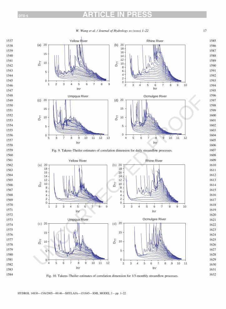
displayed in Figs. 9–11.

We cannot find any obvious scaling region from

the Figs. 9–11. Take the Yellow River for instance,

an ambiguous ln r region could be identified as

scaling region is around ln rZ7–7.5 for the three

flow series of different timescales. But in this region,

as shown in Fig. 12, the DTT increases with the

increment of the embedding dimension, which

indicates that the system under investigation is

stochastic.

TED P

lnr

Ocmulgee River

54 6 7 8 9 10

3 4 5 6 7 8 9

lnr

Rhine River

–10

–12

–8

– 6

– 4

– 2

0

lnC

(r )

–10

–12

–8

– 6

– 4

– 2

0

lnC

(r )

)

-monthly streamflow processes.

p. 1–22

1414

1415

1416

1417

1418

1419

1420

1421

1422

1423

1424

1425

1426

1427

1428

1429

1430

1431

1432

1433

1434

1435

1436

1437

1438

1439

1440

PROOF

–10

– 8

– 6

– 4

– 2

02 3 4 5 6 7 8

5 6 7 8 9 10 11 54 6 7 8 9 10

lnr

Yellow Riverln

C (

r )

–10

– 8– 9

– 6– 7

– 4– 5

– 3– 2

– 10

lnC

(r )

–10

– 8

– 6

– 4

– 2

03 4 5 6 7 8 9

lnr

Rhine River

lnC

(r )

–10

– 8

– 6

– 4

– 2

0

lnC

(r )

lnr lnr

Umpqua River Ocmulgee River

(a) (b)

(c) (d)

Fig. 8. ln C(r) versus ln r plots for monthly streamflow processes.

H



1441

1442

1443

1444

1445

1446

1447

1448

1449

1450

1451

1452

1453

1454

1455

1456

1457

1458

1459

1460

1461

1462

1463

1464

1465

1466

1467

1468

1469

1470

1471

1472

1473

1474

1475

1476

1477

1478

1479

1480

1481

1482

1483

1484

1485

1486

1487

1488

1489

1490

1491

1492

1493

1494

1495

1496

1497

1498

1499

1500

1501

1502

1503

1504

1505

1506

1507

1508

1509

1510

1511

1512

1513

1514

1515
7. Discussion
C1516

1517

1518

1519

1520

1521

1522

1523

1524

1525

1526

1527

1528

1529

1530

1531

1532

1533

1534

1535

1536

UNCORRE7.1. On the estimation of correlation dimension

Three issues regarding the estimation of corre-

lation dimension should be noticed.

First, about the minimum data size for estimating

correlation dimension. Some authors claim that the

size of 10A (Procaccia, 1988) or 10(2C0.4m) (Neren-

berg and Essex, 1990; Tsonis et al., 1993), where A is

the greatest integer smaller than correlation dimen-

sion and m is the embedding dimension, is needed for

estimating correlation dimension with an error less

than 5%. Whereas some other researchers found that

smaller data size is needed. For instance, the

minimum data points for reliable correlation dimen-

sion D is 10D/2 (Eckmann and Ruelle, 1992), orffiffiffi2

p!ffiffiffiffiffiffiffiffiffi

27:5p D

(Hong and Hong, 1994), or 5m to keep the

edge effect error in correlation dimension estimation

below 5% (Theiler, 1990), and empirical results of

dimension calculations are not substantially altered by

going from 3000 or 6000 points to subsets of 500


TEDpoints (Abraham et al., 1986). In our study, data

length is long enough for estimating correlation

dimension for daily flow, but the data size used for

monthly streamflow analysis seems short, especially

the size of 540 points of monthly flow series of the

Yellow River. However, as shown in Figs. 6–11, there

is no significant difference among the behavior of

correlation integrals of the flow series with different

sampling frequency. The agreement among the

behavior of correlation integrals for daily, 1/3-

monthly and monthly flow series indicates that the

dimension calculations are very close to each other,

therefore it is possible to make basically reliable

correlation dimension calculation with a series of size

as short as 540, which is consistent with the empirical

result of Abraham et al. (1986) and satisfying the

theoretical minimum size of Hong and Hong (1994) if

the dimension is less than 3.58.

Second, about scaling region. Some authors do not

provide scaling plot when investigating the existence

of chaos (e.g. Jayawardena and Lai, 1994; Sivakumar

et al., 1999; Elshorbagy et al., 2002), whereas some

. 1–22

UNCORRECTED PROOF

0

5

10

15

20

1 2 3 4 5 6 7 8 9 2 3 4 5 6 7 8 9 10

DT

T

0

5

10

15

20

DT

T

DT

TD

TT

02468

101214161820

0

5

10

15

20

lnr

5 6 7 8 9 10 11 12 13 4 5 6 7 8 9 10 11 12

Yellow River

lnr

Rhine River

lnr

Umpqua River

lnr

Ocmulgee River

(a) (b)

(c) (d)

Fig. 9. Takens–Theiler estimates of correlation dimension for daily streamflow processes.

1 2 3 4 5 6 7 8 9

DT

T

02468

101214161820

DT

T

02468

101214161820

lnr

Yellow River

2 3 4 5 6 7 8 9 10

lnr

Rhine River

2 3 4 5 6 7 8 9 10 11

lnr

Ocmulgee River

0

5

10

15

20

DT

T

0

5

10

15

20

DT

T

4 5 6 7 8 9 10 11 12

lnr

Umpqua River

(a) (b)

(c) (d)

Fig. 10. Takens–Theiler estimates of correlation dimension for 1/3-monthly streamflow processes.




1537

1538

1539

1540

1541

1542

1543

1544

1545

1546

1547

1548

1549

1550

1551

1552

1553

1554

1555

1556

1557

1558

1559

1560

1561

1562

1563

1564

1565

1566

1567

1568

1569

1570

1571

1572

1573

1574

1575

1576

1577

1578

1579

1580

1581

1582

1583

1584

1585

1586

1587

1588

1589

1590

1591

1592

1593

1594

1595

1596

1597

1598

1599

1600

1601

1602

1603

1604

1605

1606

1607

1608

1609

1610

1611

1612

1613

1614

1615

1616

1617

1618

1619

1620

1621

1622

1623

1624

1625

1626

1627

1628

1629

1630

1631

1632

H



1633

1634

1635

1636

1637

1638

1639

1640

1641

1642

1643

1644

1645

1646

1647

1648

1649

1650

1651

1652

1653

1654

1655

1656

1657

1658

1659

1660

1661

1662

1663

1664

1665

1666

1667

1668

1669

1670

1671

1672

1673

1674

1675

1676

1677

1678

1679

1680

1681

1682

1683

1684

1685

1686

1687

1688

1689

1690

1691

1692

1693

1694

1695

1696

1697

1698

1699

1700

1701

1702

other authors provide scaling plot, but give no

obvious scaling region (e.g. Porporato and Ridolfi

1996). However, a clearly discernible scaling region

is crucial to make a convincing and reliable estimate

of correlation dimension (Kantz and Schreiber, 1997)

.

Third, about temporally related points for comput-

ing C(r). To exclude temporally related points from

the computation of C(r), the Theiler window as in Eq.

(5) is indispensable. Grassberger (1990) remarked that

when estimating the dimension of an attractor from a

time sequence, one has to make sure that there exist no

dynamical correlations between data points, so that all

correlations are due to the geometry of the attractor

rather than due to short-time correlations. He urged

the reader to be very generous with the Theiler

window parameter. Because streamflow series is

highly temporally related, especially for daily flow,

therefore, without setting Theiler window w, we

would find a spurious scaling region between ln r Z5–7 in the plot of DTT versus ln r which gives

an incorrect estimate of correlation dimension.

UNCORREC1 2 3 4 5 6 7 8 9

lnr

Yellow River

0

5

10

15

20

0

5

10

15

20

4 5 6 7 8 9 10 11

lnr

Umpqua River

DT

TD

TT

(a) (b

(c) (d

Fig. 11. Takens–Theiler estimates of correlation d


ROOF

This problem has been pointed out by Wilcox et al.

(1991) a decade ago, however, some authors ignored

this (e.g. Elshorbagy et al., 2002), and some others

take a very small Theiler window, which is maybe not

large enough to exclude temporal correlations

between the points (for example, Porporato and

Ridolfi (1996) take wZ5 for daily flow series).

Fig. 13 shows the Takens–Theiler’s estimate for

daily streamflow series of the four rivers with w set to

be 0. It is clear that with wZ0, we would find spurious

scaling regions in all these plots. Furthermore,

comparing the plots for the daily streamflow of the

Rhine river with different values of w, namely,

Figs. 13(b), 14(a) and (b), we can further find that

the smaller the value of w, the lower the estimated

correlation dimension. According to these plots, when

wZ0, the correlation dimensionD is less than 4; when

wZ5, D is less than 8, and when wZ15, D is less than

10. Therefore, the dimension estimate could be

seriously too low if temporal coherence in the time

series is mistaken for geometrical structure (Kantz

and Schreiber, 1997).

TED P

1 2 3 4 5 6 7 8 9

lnr

Rhine River

0

5

10

15

20

0

5

10

15

20

2 3 4 5 6 7 8 9 10

lnr

Ocmulgee River

DT

TD

TT

)

)

imension for monthly streamflow processes.

. 1–22

1703

1704

1705

1706

1707

1708

1709

1710

1711

1712

1713

1714

1715

1716

1717

1718

1719

1720

1721

1722

1723

1724

1725

1726

1727

1728

0

1

2

3

4

5

6

0 2 4 6 8 10 12 14 16 18 20

Embedding dimension

DT

T

1/3-monthly flowmonthly flow

Daily flow

Fig. 12. Relationship between DTT and embedding dimension for

streamflow of the Yellow River.



1729

1730

1731

1732

1733

1734

1735

1736

1737

1738

1739

1740

1741

1742

1743

1744

1745

1746

1747

1748

1749

1750

1751

1752

1753

1754

1755

1756

1757

1758

1759

1760

1761

1762

1763

1764

1765

1766

1767

1768

1769

1770

1771

1772

1773

1774

1775

1776

1777

1778

1779

1780

1781

1782

1783

1784

1785

1786

1787

1788

1789

1790

1791

1792

1793

1794

1795

1796

1797

1798

1799

7.2. On the sources of nonlinearity

Streamflow processes are fundamentally driven by

meteorological processes. Because daily meteorolo-

gical series are usually nonlinear (e.g. Rao and Yu,

1990), and the daily streamflow process is usually

perceived as nonlinearly dependent on the magnitude

of the rainfall (e.g. Minshall, 1960; Wang et al., 1981)

, therefore, the major source of nonlinearity in daily

streamflow processes probably stems from the

nonlinearity in daily precipitation and temperature

processes, and nonlinear rainfall-runoff response

UNCORREC1 2 3 4 5 6 7 8 9

DT

T

02468

101214161820

DT

T

02468

101214161820

lnr

Yellow River

5 6 7 8 9 10 11 12 13

lnr

Umpqua River

(a) (b

(c) (d

Fig. 13. Takens–Theiler estimates without consid


PROOF

make the nonlinearity of streamflow processes more

complicated.

As the timescale increase, the nonlinearity in the

meteorological series weakens. For example, Chen

and Rao (2003) found that all of the stationary

segments of standardized monthly temperature and

precipitation series they studied are either Gaussian or

linear. One the other hand, nonlinear fluctuations,

such as the ARCH (autoregressive conditional

heteroskedasticity) effect in daily streamflow pro-

cesses (Wang et al., 2004), that exhibits in the daily

streamflow processes are generalized, therefore, the

nonlinearity in streamflow processes weakens with

increasing timescale.

However, because of differences in the geographi-

cal and climatological environment, the character and

intensity of nonlinearity of different streamflow

systems are consequently different. For example,

temperature may be a dominant variable for the

whole dynamics of the streamflow process of the

Yellow River at Tangnaihai. Its effect on both rainfall

and snow cover has a very strong influence in

determining the inertia of the whole hydrological

TED

DT

T

02468

101214161820

DT

T

02468

101214161820

2 3 4 5 6 7 8 9 10

lnr

Rhine River

4 5 6 7 8 9 10 11 12

lnr

Ocmulgee River

)

)

ering Theiler window for daily streamflow.

p. 1–22

1800

1801

1802

1803

1804

1805

1806

1807

1808

1809

1810

1811

1812

1813

1814

1815

1816

1817

1818

1819

1820

1821

1822

1823

1824

C

2 3 4 5 6 7 8 9 10

DT

T

02468

101214161820

lnr

2 3 4 5 6 7 8 9 10

lnr

(a)

DT

T

02468

101214161820(b)

Fig. 14. Takens–Theiler estimates with small Theiler window for daily streamflow of the Rhine River. (a) wZ5; (b) wZ15.

H



1825

1826

1827

1828

1829

1830

1831

1832

1833

1834

1835

1836

1837

1838

1839

1840

1841

1842

1843

1844

1845

1846

1847

1848

1849

1850

1851

1852

1853

1854

1855

1856

1857

1858

1859

1860

1861

1862

1863

1864

1865

1866

1867

1868

1869

1870

1871

1872

1873

1874

1875

1876

1877

1878

1879

1880

1881

1882

1883

1884

1885

1886

1887

1888

1889

1890

1891

1892

1893

1894

1895

1896

1897

1898

1899

1900

1901

1902

1903

1904

1905

1906

1907

1908

1909

1910

1911

1912
ORRE
system. That probably makes the streamflow system

of the Yellow River at Tangnaihai appears to be less

reactive than other streamflow systems. Even though

the system preserves a nonlinear character at short

timescale, it may disappear faster than other more

active streamflow systems as the timescale increase.

That may be the reason why only the 1/3-monthly

flow series at Tangnaihai can exhibit linearity after

being standardized by seasonal variance.

Another aspect should be noticed is the nonlinear-

ity of streamflow response with respect to the

catchment characteristics (e.g. area, topography and

groundwater system). A number of studies indicate

that the nonlinearity decreases and catchments

become more linear with increasing catchment area

(Minshall, 1960; Wang et al., 1981). However,

nonlinearity does not disappear as the catchment

scale increase because channel network hydrodyn-

amics would be an important source of nonlinearity at

large scales (Robinson et al., 1995). Among the

streamflow processes of 4 rivers in our study,

streamflow processes of the Yellow River and the

Rhine River with much larger catchment area seem

possess no less nonlinearity in terms of BDS statistics

than streamflow processes of the other two rivers with

smaller catchment area, namely, no clear relationship

is found between the catchment area and the intensity

of nonlinearity.
C 1913
1914

1915

1916

1917

1918

1919

1920

UN8. Conclusions

Streamflow processes are commonly considered as

nonlinear. However, it is not clear what kind of

nonlinearity is acting underlying the streamflow


TED PROOFprocesses and how strong the nonlinearity is within

the streamflow processes at different timescales.

Streamflow processes of four rivers, namely, the

Yellow River at Tangnaihai, the Rhine River at

Lobith, the Umpqua River near Elkton and the

Ocmulgee River at Macon are tested for nonlinearity

with BDS test (Brock et al., 1996). The tests focus on

four characteristic time scales (i.e. one year, one

month, 1/3 month and one day). All the series (except

annual series) are pre-processed in two ways, namely,

logarithmization (referred to as Log), and logarith-

mization-and-deseasonalization (referred to as Log-

DS). Then the pre-processed series are pre-whitened

with AR models. It is found that all annual series are

linear. Log-DS monthly flow series of the Rhine River

and the Ocmulgee River as well as Log monthly flow

series of the Ocmulgee River are also basically linear.

But all the daily series, 1/3-monthly series and other

monthly streamflow series cannot pass the BDS test,

indicating the existence of nonlinearity in these series.

And the shorter the timescale is, the stronger the

nonlinearity. After being standardized with seasonal

variance, while those series that are linear before

standardization pass the BDS test with generally

higher p-values, indicating stronger linearity, Log

monthly series of the Rhine and the Log-DS monthly

and the 1/3-montly series of the Yellow River also

pass the BDS test, indicating that seasonal variation in

the variance of the pre-whitened series may dominate

the nonlinearity in these series. But other series,

especially daily series, still exhibit strong nonlinear-

ity, although the BDS statistic values are smaller than

those for un-standardized series, which indicates the

decrease of the intensity of nonlinearity with

standardization. However, we cannot conclude that

there is no nonlinearity present in those 1/3-monthly

. 1–22



1921

1922

1923

1924

1925

1926

1927

1928

1929

1930

1931

1932

1933

1934

1935

1936

1937

1938

1939

1940

1941

1942

1943

1944

1945

1946

1947

1948

1949

1950

1951

1952

1953

1954

1955

1956

1957

1958

1959

1960

1961

1962

1963

1964

1965

1966

1967

1968

1969

1970

1971

1972

1973

1974

1975

1976

1977

1978

1979

1980

1981

1982

1983

1984

1985

1986

1987

1988

1989

1990

1991

and monthly streamflow series which pass BDS test,

because the power analysis of BDS test shows that

BDS test is not powerful enough for detecting weak

nonlinearity.

There is no evidence found of the existence of low-

dimensional chaos in the streamflow series of all the

four rivers with correlation exponent method. When

testing for chaos in streamflow processes, some

authors tend to accept the existence of chaos in

streamflow processes even if test results do not give

really clear evidences. For instance, many published

research results claim clear evidences of the existence

of low-dimensional chaos in streamflow series with-

out providing scaling plots or without providing

convincing scaling plots with clearly discernible

scaling regions, whereas clearly discernible scaling

region is imperative for identifying the finite

correlation dimension. Furthermore, cares must be

taken when computing correlation dimension for

serially dependent hydrological series, because tem-

poral coherence could be mistaken for geometrical

structure if temporally correlated points are not

excluded for calculating correlation integrals.

1992

1993

1994

1995

1996

1997

9. Uncited references

Box and Jenkins (1976); Hinich, (1982); Shi-

Zhong and Shi-Ming (1994); McLeod and Li (1984).

C 1998

1999

2000

2001

2002

2003

2004

2005

2006

2007

2008

2009

2010

2011

2012

2013

2014

2015

2016

UNCORREAcknowledgements

W. Wang is very grateful for the financial support

he received from the Swiss National Science

Foundation, SCOPES partner countries to attend the

Hydrofractals ’03 conference in Ascona, Switzerland.

Prof. P. Burlando and Ms. Lynda Dowse are also very

gratefully acknowledged for their kind support and

hospitality. The comments of Professor A.R. Rao and

especially the detailed comments of an anonymous

referee help to improve the paper greatly. In addition,

the Yellow River Conservancy Commission in China

is acknowledged for providing the data of the Yellow

River, the Global Runoff Data Centre (GRDC) in

Germany for the data of the Rhine River, and the

USGS in the United States for the data of the Umpqua

and Ocmulgee River.


TED PROOF

References

Abraham, N.B., Albano, A.M., Das, B., et al., 1986. Calculating the

dimension of attractors from small data. Phys. Lett. A 114,

217–221.

Bordignon, S., Lisi, F., 2000. Nonlinear analysis and prediction of

river flow time series[J]. Environmetrics 11, 463–477.

Box, G.E.P., Jenkins, G.M., 1976. Time Series Analysis:

Forecasting and Control, second ed. Holden-Day, San

Francisco.

Brock, W.A., Hsieh, D.A., LeBaron, B., 1991. Nonlinear Dynamics,

Chaos, and Instability: Statistical Theory and Economic

Evidence. The MIT Press, Cambridge, MA.

Brock, W.A., Dechert, W.D., Scheinkman, J.A., LeBaron, B., 1996.

A test for independence based on the correlation dimension.

Econ. Rev. 15 (3), 197–235.

Chen, H.L., Rao, A.R., 2003. Linearity analysis on stationary

segments of hydrologic time series. J. Hydrol. 277, 89–99.

Dickey, D.A., Fuller, W.A., 1979. Distribution of the estimators for

autoregressive time series with a unit root. J. Am. Stat. Assoc.

74, 423–431.

Eckmann, J.P., Ruelle, D., 1992. Fundamental limitations for

estimating dimensions and Lyapunov exponents in dynamical

systems. Phys. D 56, 185–187.

Elshorbagy, A., Simonovic, S.P., Panu, U.S., 2002. Estimation of

missing stream flow data using principles of chaos theory.

J. Hydrol. 255, 125–133.

Farmer, D.J., Sidorowich, J.J., 1987. Predicting chaotic time series.

Phys. Rev. Lett. 59, 845–848.

Fraser, A.M., Swinney, H.L., 1986. Independent coordinates for

strange attractors from mutual information. Phys. Rev. A 33 (2),

1134–1140.

Ghilardi, P., Rosso, R., 1990. Comment on chaos in rainfall. Water

Resour. Res. 26 (8), 1837–1839.

Gimeno, R., Manchado, B., Minguez, R., 1999. Stationarity tests for

financial time series. Phys. A 269, 72–78.

Grassberger, P., 1990. An optimized box-assisted algorithm for

fractal dimensions. Phys. Lett. A 148, 63–68.

Grassberger, P., Procaccia, I., 1983a. Measuring the strangeness of

strange attractors. Phys. D 9, 189–208.

Grassberger, P., Procaccia, I., 1983b. Estimation of the Kolmogorov

entropy from a chaotic signal. Phys. Rev. A 28, 2591–2593.

Hegger, R., Kantz, H., Schreiber, T., 1999. Practical implemen-

tation of nonlinear time series methods: the TISEAN package.

Chaos 9, 413–435.

Henon, M., 1976. A two-dimensional mapping with a strange

attractor. Commun. Math. Phys. 50 (1), 69–77.

Hinich, M.J., 1982. Testing for Gaussianity and linearity of a

stationary time series. J. Time Ser. Anal. 3 (3), 169–176.

Shi-Zhong, Hong, Shi-Ming, Hong, 1994. An amendment to the

fundamental limits on dimension calculations. Fractals 2 (1),

123–125.

Islam, M.N., Sivakumar, B., 2002. Characterization and prediction

of runoff. Dynamics: a nonlinear dynamical view. Adv. Water

Res. 25, 179–190.

Jayawardena, A.W., Lai, F., 1994. Analysis and prediction of chaos

in rainfall and stream flow time series. J. Hydrol. 153, 23–52.

p. 1–22

C

H



2017

2018

2019

2020

2021

2022

2023

2024

2025

2026

2027

2028

2029

2030

2031

2032

2033

2034

2035

2036

2037

2038

2039

2040

2041

2042

2043

2044

2045

2046

2047

2048

2049

2050

2051

2052

2053

2054

2055

2056

2057

2058

2059

2060

2061

2062

2063

2064

2065

2066

2067

2068

2069

2070

2071

2072

2073

2074

2075

2076

2077

2078

2079

2080

2081

2082

2083

2084

2085

2086

2087

2088

2089

2090

2091

2092

2093

2094

2095

2096

2097

2098

2099

2100

2101

2102
RRE
Kantz, H., Schreiber, T., 1997. Nonlinear Time Series Analysis.

Cambridge University Press, Cambridge.

Kim, H.S., Kang, D.S., Kim, J.H., 2003. The BDS statistic and

residual test. Stochast. Environ. Res. Risk Assess. 17, 104–115.

Koutsoyiannis, D., Pachakis, D., 1996. Deterministic chaos versus

stochasticity in analysis and modeling of point rainfall series.

J. Geophys. Res. 101 (D21), 26441–26451.

Kwiatkowski, D., Phillips, P.C.B., Schmidt, P., Shin, Y., 1992.

Testing the null of stationarity against the alternative of a unit

root: How sure are we that economic time series have a unit

root? J. Econometrics 54, 159–178.

McLeod, A.I., Li, W.K., 1984. Diagnostic checking ARMA time

series models using squared residual autocorrelations. J. Time

Ser. Anal. 4, 269–273.

Minshall, N.E., 1960. Predicting storm runoff on small experimental

watershed. J. Hydraul. Div. Am. Soc. Eng. 86, 17–38.

Nerenberg, M.A.H., Essex, C., 1990. Correlation dimension and

systematic geometric effects. Phys. Rev. A 42 (12), 7065–7074.

Packard, N.H., Crutchfield, J.P., Farmer, J.D., Shaw, R.S., 1980.

Geometry from a time series. Phys. Rev. Lett. 45 (9), 712–716.

Pasternack, G.B., 1999. Does the river run wild? Assessing chaos in

hydrological systems. Adv. Water Resour. 23, 253–260.

Patterson, D.M., Ashley, R.A., 2000. A Nonlinear Time Series

Workshop: A Toolkit for Detecting and Identifying Nonlinear

Serial Dependence. Kluwer Academic, Boston.

Porporato, A., Ridolfi, L., 1997. Nonlinear analysis of river flow

time sequences. Water Resour. Res. 33 (6), 1353–1367.

Procaccia, I., 1988. Complex or just complicated? Nature 333,

498–499.

Rao, A.R., Yu, G.-H., 1990. Gaussianity and linearity tests of

hydrologic time series. Stochast. Hydrol. Hydraul. 4, 121–134.

Robinson, J.S., Sivapalan, M., Snell, J.D., 1995. On the relative

roles of hillslop processes, channel routing and network

geomorphology in the hydrologic response of natural catch-

ments. Water Resour. Res. 31 (12), 3089–3101.

Rogers, W.F., 1980. A practical method for linear and nonlinear

runoff. J. Hydrol. 46, 51–78.

Rogers, W.F., 1982. Some characteristics and implications of

drainage basin linearity and nonlinearity. J. Hydrol. 55,

247–265.

Rogers, W.F., Zia, H.A., 1982. Linear and nonlinear runoff from

large drain basins. J. Hydrol. 55, 267–278.

Sauer, T., Yorke, J.A., 1993. How many delay coordinates do you

need? Int. J. Bif. Chaos 3, 737–744.

Schreiber, T., Schmitz, A., 1996. Improved surrogate data for

nonlinearity tests. Phys. Rev. Lett. 77 (4), 635–638.

UNCO


TED PROOF

Schertzer, D., Tchiguirinskaia, I., Lovejoy, S., Hubert, P.,

Bendjoudi, H., et al., 2002. Which chaos in the rainfall-

runoff process? A discussion on Evidence of chaos in the

rainfall-runoff process by Sivakumar. Hydrol. Sci. J. 47 (1),

139–147.

Schwert, G.W., 1989. Tests for unit roots: A monte Carlo

investigation. J. Bus. Eco. Stat. 7, 147–159.

Sivakumar, B., Liong, S.-Y., Liaw, C.-Y., Phoon, K.-K., 1999.

Singapore rainfall behavior: chaotic? J. Hydrol. Eng. 4 (1),

38–48.

Sugihara, G., May, R.M., 1990. Nonlinear forecasting as a way of

distinguishing chaos from measurement error in time series.

Nature 344, 734–741.

Takens, F., 1981. Detecting strange attractors in turbulence. Lecture

Notes Math. 898, 366–381.

Theiler, J., 1986. Spurious dimension from correlation algorithms

applied to limited time-series data. Phys. Rev. A 34 (3), 2427–

2432.

Theiler, J., 1990. Estimating fractal dimension. J. Opt. Soc. Am. A

7, 1055–1073.

Theiler, J., Eubank, S., 1993. Don’t bleach chaotic data. Chaos 3,

771–782.

Theiler, J., Eubank, S., Longtin, A., Galdrikian, B., Farmer, J.D.,

1992. Testing for nonlinearity in time series: the method of

surrogate data. Phys. D 58, 77–94.

Tsonis, A.A., 2001. Probing the linearity and nonlinearity in the

transitions of the atmospheric circulation. Nonlinear Processes

Geophysics 8, 341–345.

Tsonis, A.A., Elsner, J.B., Georgakakos, K.P., 1993. Estimating the

dimension of weather and climate attractors: important issues

about the procedure and interpretation. J. Atmos. Sci. 50 (15),

2549–2555.

Wang, C.T., Gupta, V.K., Waymire, E., 1981. A geomorphologic

synthesis of nonlinearity in surface runoff. Water Resour. Res.

19 (3), 545–554.

Wang, W., Van Gelder P.H.A.J.M., Vrijling, J.K., Ma, J. 2004.

Testing and modelling autoregressive conditional heteroskedas-

ticity of streamflow processes. submitted to Nonlinear Proc.

Geophy.

Wilcox, B.P., Seyfried, M.S., Matison, T.H., 1991. Searching for

chaotic dynamics in snowmelt runoff. Water Resour. Res. 27 (6)

, 1005–1010.

Wolf, A., Swift, J.B., Swinney, H.L., Vastano, A., 1985.

Determining Lyapunov exponents from a time series. Phys. D

16, 285–317.

. 1–22

2103

2104

2105

2106

2107

2108

2109

2110

2111

2112

ARTICLE IN PRESS - d1rkab7tlqy5f1.cloudfront.net faculteit/Afdelingen... · UNCORRECTED PROOF...

Documents

Transcript of ARTICLE IN PRESS - d1rkab7tlqy5f1.cloudfront.net faculteit/Afdelingen... · UNCORRECTED PROOF...