
Artificial Intelligence Approximately every other Tuesday. · Artificial Intelligence Prof. Dr....
190
Artificial Intelligence Prof. Dr. Jürgen Dix Department of Informatics TU Clausthal Summer 2009 Prof. Dr. Jürgen Dix · Department of Informatics, TU Clausthal Artificial Intelligence, SS 09 1 Time and place: Tuesday and Wednesday 10–12 in Multimediahörsaal (Tannenhöhe) Exercises: Approximately every other Tuesday. Website http://cig.in.tu-clausthal.de/index.php?id=163 Visit regularly! There you will find important information about the lecture, documents, exercises et cetera. Organization: Exercise: W. Jamroga, N. Bulling Exam: 23. July 2009, 13ct Prof. Dr. Jürgen Dix · Department of Informatics, TU Clausthal Artificial Intelligence, SS 09 2 History This course evolved over the last 13 years. It was first held in Koblenz (WS 95/96, WS 96/97), then in Vienna (Austria, WS 98, WS00) , Bahia Blanca (Argentina, SS 98, SS 01) and Clausthal (SS 04–08). Most chapters (except 4, 5, 7, 8 and 9) are based on the seminal book of Russel/Norvig: Artificial Intelligence. Thanks to Nils, Tristan, Wojtek for the time they invested in crafting slides, transforming to beamertex and the exercises. Their help over the years improved the course a lot. Prof. Dr. Jürgen Dix · Department of Informatics, TU Clausthal Artificial Intelligence, SS 09 3 Lecture Overview 1. Introduction 2. Searching 3. Supervised Learning 4. Knowledge Engineering: SL 5. Hoare Calculus 6. Knowledge Engineering: FOL 7. Knowledge Engineering: Provers 8. Planning 9. Nonmonotonic Reasoning Prof. Dr. Jürgen Dix · Department of Informatics, TU Clausthal Artificial Intelligence, SS 09 4
Transcript of Artificial Intelligence Approximately every other Tuesday. · Artificial Intelligence Prof. Dr....
Artificial Intelligence
Prof. Dr. Jürgen Dix
Department of InformaticsTU Clausthal
Summer 2009
Prof. Dr. Jürgen Dix · Department of Informatics, TU Clausthal Artificial Intelligence, SS 09 1
Time and place: Tuesday and Wednesday 10–12in Multimediahörsaal (Tannenhöhe)Exercises: Approximately every other Tuesday.
Websitehttp://cig.in.tu-clausthal.de/index.php?id=163
Visit regularly!
There you will find important information aboutthe lecture, documents, exercises et cetera.
Organization: Exercise: W. Jamroga, N. BullingExam: 23. July 2009, 13ct
Prof. Dr. Jürgen Dix · Department of Informatics, TU Clausthal Artificial Intelligence, SS 09 2
HistoryThis course evolved over the last 13 years. It was first held in Koblenz(WS 95/96, WS 96/97), then in Vienna (Austria, WS 98, WS00) , BahiaBlanca (Argentina, SS 98, SS 01) and Clausthal (SS 04–08).Most chapters (except 4, 5, 7, 8 and 9) are based on the seminal book ofRussel/Norvig: Artificial Intelligence.
Thanks to Nils, Tristan, Wojtek for the time they invested incrafting slides, transforming to beamertex and the exercises. Theirhelp over the years improved the course a lot.
Prof. Dr. Jürgen Dix · Department of Informatics, TU Clausthal Artificial Intelligence, SS 09 3
Lecture Overview1. Introduction2. Searching3. Supervised Learning4. Knowledge Engineering: SL5. Hoare Calculus6. Knowledge Engineering: FOL7. Knowledge Engineering: Provers8. Planning9. Nonmonotonic Reasoning
Prof. Dr. Jürgen Dix · Department of Informatics, TU Clausthal Artificial Intelligence, SS 09 4
1 Introduction
1. Introduction1 Introduction
What Is AI?From Plato To ZuseHistory of AIIntelligent Agents
Prof. Dr. Jürgen Dix · Department of Informatics, TU Clausthal Artificial Intelligence, SS 09 5
1 Introduction
Content of this chapter (1):
Defining AI: There are several definitions of AI. They leadto several scientific areas ranging from CognitiveScience to Rational Agents.
History: We discuss some important philosophical ideasin the last 3 millennia and touch several eventsthat play a role in later chapters (syllogisms ofAristotle, Ockhams razor, Ars Magna).
AI since 1958: AI came into being in 1956-1958 with JohnMcCarthy. We give a rough overview of itssuccesses and failures.
Prof. Dr. Jürgen Dix · Department of Informatics, TU Clausthal Artificial Intelligence, SS 09 6
1 Introduction
Content of this chapter (2):
Rational Agent: The modern approach to AI is based onthe notion of a Rational Agent that is situated inan environment. We discuss the PEASdescription and give some formal definitions ofagency, introducing the notions of run,standard- vs. state- based agent
Prof. Dr. Jürgen Dix · Department of Informatics, TU Clausthal Artificial Intelligence, SS 09 7
1 Introduction1.1 What Is AI?
1.1 What Is AI?
Prof. Dr. Jürgen Dix · Department of Informatics, TU Clausthal Artificial Intelligence, SS 09 8
1 Introduction1.1 What Is AI?
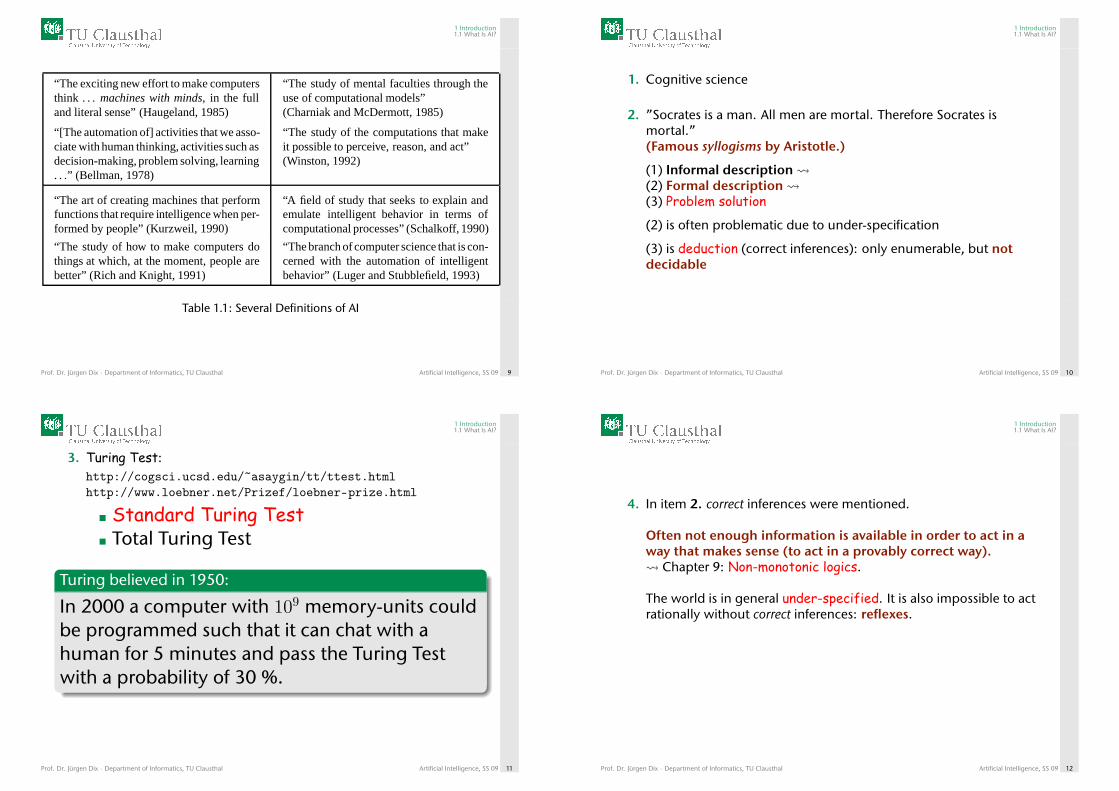
“The exciting new effort to make computersthink . . . machines with minds, in the fulland literal sense” (Haugeland, 1985)
“The study of mental faculties through theuse of computational models”(Charniak and McDermott, 1985)
“[The automation of] activities that we asso-ciate with human thinking, activities such asdecision-making, problem solving, learning. . .” (Bellman, 1978)
“The study of the computations that makeit possible to perceive, reason, and act”(Winston, 1992)
“The art of creating machines that performfunctions that require intelligence when per-formed by people” (Kurzweil, 1990)
“A field of study that seeks to explain andemulate intelligent behavior in terms ofcomputational processes” (Schalkoff, 1990)
“The study of how to make computers dothings at which, at the moment, people arebetter” (Rich and Knight, 1991)
“The branch of computer science that is con-cerned with the automation of intelligentbehavior” (Luger and Stubblefield, 1993)
Table 1.1: Several Definitions of AI
Prof. Dr. Jürgen Dix · Department of Informatics, TU Clausthal Artificial Intelligence, SS 09 9
1 Introduction1.1 What Is AI?
1. Cognitive science
2. ”Socrates is a man. All men are mortal. Therefore Socrates ismortal.”(Famous syllogisms by Aristotle.)
(1) Informal description (2) Formal description (3) Problem solution
(2) is often problematic due to under-specification
(3) is deduction (correct inferences): only enumerable, but notdecidable
Prof. Dr. Jürgen Dix · Department of Informatics, TU Clausthal Artificial Intelligence, SS 09 10
1 Introduction1.1 What Is AI?
3. Turing Test:http://cogsci.ucsd.edu/~asaygin/tt/ttest.htmlhttp://www.loebner.net/Prizef/loebner-prize.html
Standard Turing TestTotal Turing Test
Turing believed in 1950:
In 2000 a computer with 109 memory-units couldbe programmed such that it can chat with ahuman for 5 minutes and pass the Turing Testwith a probability of 30 %.
Prof. Dr. Jürgen Dix · Department of Informatics, TU Clausthal Artificial Intelligence, SS 09 11
1 Introduction1.1 What Is AI?
4. In item 2. correct inferences were mentioned.
Often not enough information is available in order to act in away that makes sense (to act in a provably correct way). Chapter 9: Non-monotonic logics.
The world is in general under-specified. It is also impossible to actrationally without correct inferences: reflexes.
Prof. Dr. Jürgen Dix · Department of Informatics, TU Clausthal Artificial Intelligence, SS 09 12
1 Introduction1.1 What Is AI?
To pass the total Turing Test, the computer will need:computer vision to perceive objects,robotics to move them about.
The question Are machines able to think? leads to 2 theses:Weak AI thesis: Machines can be built, that act as if they wereintelligent.Strong AI thesis: Machines that act in an intelligent way do possesscognitive states, i.e. mind.
Prof. Dr. Jürgen Dix · Department of Informatics, TU Clausthal Artificial Intelligence, SS 09 13
1 Introduction1.1 What Is AI?
The Chinese Chamberwas used in 1980 by Searle to demonstrate that a system can pass theTuring Test but disproves the Strong AI Thesis. The chamberconsists of:
CPU: an English-speaking man without experienceswith the Chinese language,Program: a book containing rules formulated in Englishwhich describe how to translate Chinese texts,Memory: sufficient pens and paper
Papers with Chinese texts are passed to the man, which hetranslates using the book.
Question
Does the chamber understand Chinese?
Prof. Dr. Jürgen Dix · Department of Informatics, TU Clausthal Artificial Intelligence, SS 09 14
1 Introduction1.2 From Plato To Zuse
1.2 From Plato To Zuse
Prof. Dr. Jürgen Dix · Department of Informatics, TU Clausthal Artificial Intelligence, SS 09 15
1 Introduction1.2 From Plato To Zuse
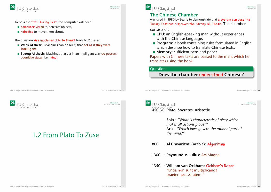
450 BC: Plato, Socrates, Aristotle
Sokr.: ”What is characteristic of piety whichmakes all actions pious?”Aris.: ”Which laws govern the rational part ofthe mind?”
800 : Al Chwarizmi (Arabia): Algorithm
1300 : Raymundus Lullus: Ars Magna
1350 : William van Ockham: Ockham’s Razor”Entia non sunt multiplicandapraeter necessitatem.”
Prof. Dr. Jürgen Dix · Department of Informatics, TU Clausthal Artificial Intelligence, SS 09 16
1 Introduction1.2 From Plato To Zuse
1596–1650: R. Descartes:Mind = physical systemFree will, dualism
1623–1662: B. Pascal, W. Schickard:Addition-machines
Prof. Dr. Jürgen Dix · Department of Informatics, TU Clausthal Artificial Intelligence, SS 09 17
1 Introduction1.2 From Plato To Zuse
1646–1716: G. W. Leibniz:Materialism, uses ideas of Ars Magna to builda machine for simulating the human mind
1561–1626: F. Bacon: Empirism
1632–1704: J. Locke: Empirism”Nihil est in intellectu quodnon antefuerat in sensu.”
1711–1776 : D. Hume: Induction
1724–1804: I. Kant:”Der Verstand schöpft seine Gesetze nichtaus der Natur, sondern schreibt sie dieser vor.”
Prof. Dr. Jürgen Dix · Department of Informatics, TU Clausthal Artificial Intelligence, SS 09 18
1 Introduction1.2 From Plato To Zuse
1805 : Jacquard: Loom
1815–1864: G. Boole:Formal language,Logic as a mathematical discipline
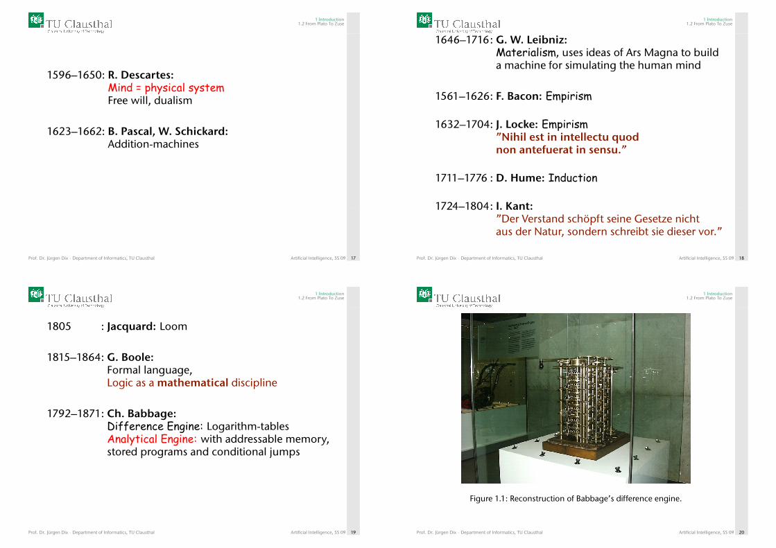
1792–1871: Ch. Babbage:Difference Engine: Logarithm-tablesAnalytical Engine: with addressable memory,stored programs and conditional jumps
Prof. Dr. Jürgen Dix · Department of Informatics, TU Clausthal Artificial Intelligence, SS 09 19
1 Introduction1.2 From Plato To Zuse
Figure 1.1: Reconstruction of Babbage’s difference engine.
Prof. Dr. Jürgen Dix · Department of Informatics, TU Clausthal Artificial Intelligence, SS 09 20
1 Introduction1.2 From Plato To Zuse
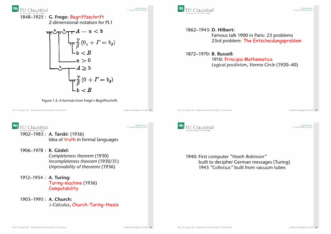
1848–1925 : G. Frege: Begriffsschrift2-dimensional notation for PL1
Figure 1.2: A formula from Frege’s Begriffsschrift.
Prof. Dr. Jürgen Dix · Department of Informatics, TU Clausthal Artificial Intelligence, SS 09 21
1 Introduction1.2 From Plato To Zuse
1862–1943: D. Hilbert:Famous talk 1900 in Paris: 23 problems23rd problem: The Entscheidungsproblem
1872–1970: B. Russell:1910: Principia MathematicaLogical positivism, Vienna Circle (1920–40)
Prof. Dr. Jürgen Dix · Department of Informatics, TU Clausthal Artificial Intelligence, SS 09 22
1 Introduction1.2 From Plato To Zuse
1902–1983 : A. Tarski: (1936)Idea of truth in formal languages
1906–1978 : K. Gödel:Completeness theorem (1930)Incompleteness theorem (1930/31)Unprovability of theorems (1936)
1912–1954 : A. Turing:Turing-machine (1936)Computability
1903–1995 : A. Church:λ-Calculus, Church-Turing-thesis
Prof. Dr. Jürgen Dix · Department of Informatics, TU Clausthal Artificial Intelligence, SS 09 23
1 Introduction1.2 From Plato To Zuse
1940: First computer ”Heath Robinson”built to decipher German messages (Turing)1943 ”Collossus” built from vacuum tubes
Prof. Dr. Jürgen Dix · Department of Informatics, TU Clausthal Artificial Intelligence, SS 09 24
1 Introduction1.2 From Plato To Zuse
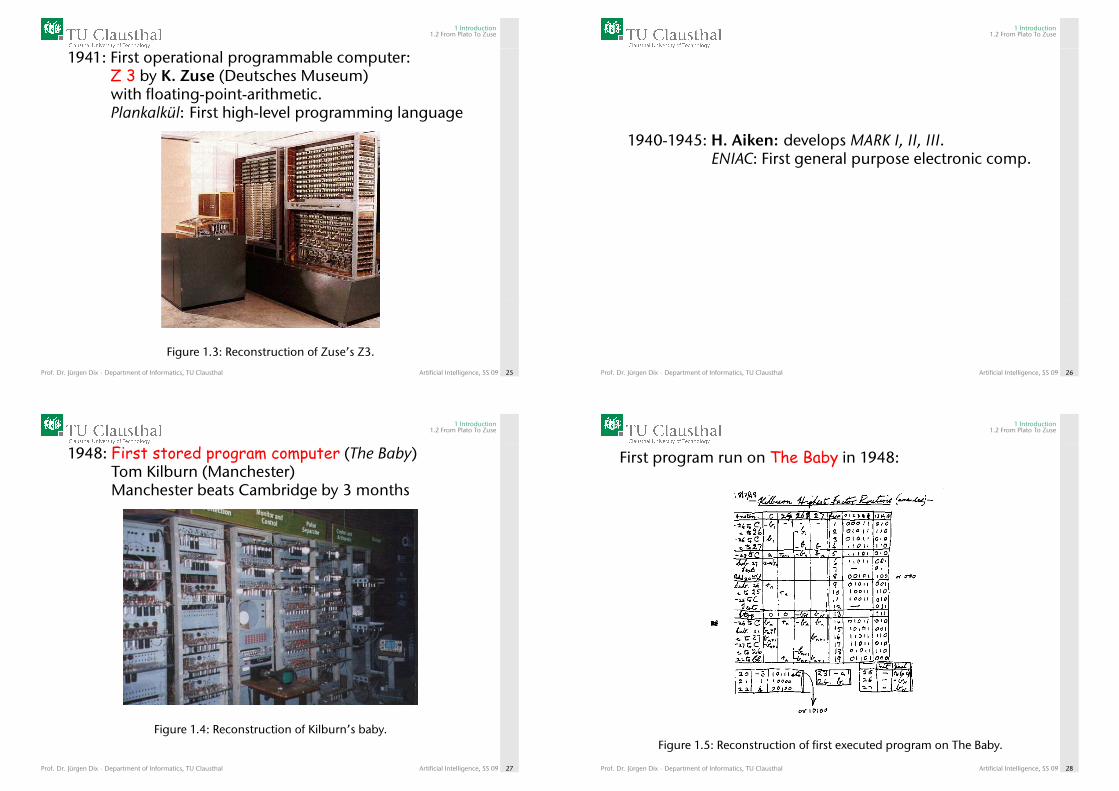
1941: First operational programmable computer:Z 3 by K. Zuse (Deutsches Museum)with floating-point-arithmetic.Plankalkül: First high-level programming language
Figure 1.3: Reconstruction of Zuse’s Z3.
Prof. Dr. Jürgen Dix · Department of Informatics, TU Clausthal Artificial Intelligence, SS 09 25
1 Introduction1.2 From Plato To Zuse
1940-1945: H. Aiken: develops MARK I, II, III.ENIAC: First general purpose electronic comp.
Prof. Dr. Jürgen Dix · Department of Informatics, TU Clausthal Artificial Intelligence, SS 09 26
1 Introduction1.2 From Plato To Zuse
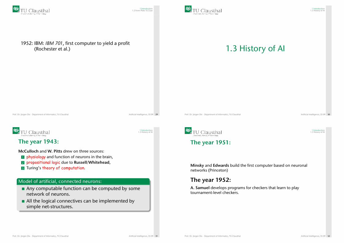
1948: First stored program computer (The Baby)Tom Kilburn (Manchester)Manchester beats Cambridge by 3 months
Figure 1.4: Reconstruction of Kilburn’s baby.
Prof. Dr. Jürgen Dix · Department of Informatics, TU Clausthal Artificial Intelligence, SS 09 27
1 Introduction1.2 From Plato To Zuse
First program run on The Baby in 1948:
Figure 1.5: Reconstruction of first executed program on The Baby.
Prof. Dr. Jürgen Dix · Department of Informatics, TU Clausthal Artificial Intelligence, SS 09 28
1 Introduction1.2 From Plato To Zuse
1952: IBM: IBM 701, first computer to yield a profit(Rochester et al.)
Prof. Dr. Jürgen Dix · Department of Informatics, TU Clausthal Artificial Intelligence, SS 09 29
1 Introduction1.3 History of AI
1.3 History of AI
Prof. Dr. Jürgen Dix · Department of Informatics, TU Clausthal Artificial Intelligence, SS 09 30
1 Introduction1.3 History of AI
The year 1943:
McCulloch and W. Pitts drew on three sources:1 physiology and function of neurons in the brain,2 propositional logic due to Russell/Whitehead,3 Turing’s theory of computation.
Model of artificial, connected neurons:Any computable function can be computed by somenetwork of neurons.All the logical connectives can be implemented bysimple net-structures.
Prof. Dr. Jürgen Dix · Department of Informatics, TU Clausthal Artificial Intelligence, SS 09 31
1 Introduction1.3 History of AI
The year 1951:
Minsky and Edwards build the first computer based on neuronalnetworks (Princeton)
The year 1952:A. Samuel develops programs for checkers that learn to playtournament-level checkers.
Prof. Dr. Jürgen Dix · Department of Informatics, TU Clausthal Artificial Intelligence, SS 09 32
1 Introduction1.3 History of AI
The year 1956:
Two-month workshop at Dartmouth organized by McCarthy, Minsky,Shannon and Rochester.
Idea:Combine knowledge about automata theory, neural nets and thestudies of intelligence (10 participants)
Prof. Dr. Jürgen Dix · Department of Informatics, TU Clausthal Artificial Intelligence, SS 09 33
1 Introduction1.3 History of AI
Newell und Simon show a reasoning program,the Logic Theorist, able to prove most of thetheorems in Chapter 2 of the PrincipiaMathematica (even one with a shorter proof).
But the Journal of Symbolic Logic rejected a paperauthored by Newell, Simon and Logical Theorist.Newell and Simon claim to have solved thevenerable mind-body problem.
Prof. Dr. Jürgen Dix · Department of Informatics, TU Clausthal Artificial Intelligence, SS 09 34
1 Introduction1.3 History of AI
The term Artificial Intelligence is proposed asthe name of the new discipline.
Logic Theorist is followed by the General Problem Solver, which wasdesigned from the start to imitate human problem-solving protocols.
Prof. Dr. Jürgen Dix · Department of Informatics, TU Clausthal Artificial Intelligence, SS 09 35
1 Introduction1.3 History of AI
The year 1958: Birthyear of AI
McCarthy joins MIT and develops:
1 Lisp, the dominant AI programming language2 Time-Sharing to optimize the use of computer-time3 Programs with Common-Sense.
Advice-Taker: A hypothetical program that can be seenas the first complete AI system. Unlike others itembodies general knowledge of the world.
Prof. Dr. Jürgen Dix · Department of Informatics, TU Clausthal Artificial Intelligence, SS 09 36

1 Introduction1.3 History of AI
The year 1959:
H. Gelernter: Geometry Theorem Prover
Prof. Dr. Jürgen Dix · Department of Informatics, TU Clausthal Artificial Intelligence, SS 09 37
1 Introduction1.3 History of AI
The years 1960-1966:
McCarthy concentrates on knowledge-representation and reasoning informal logic ( Robinson’s Resolution, Green’s Planner, Shakey).
Minsky is more interested in getting programs to work and focusses onspecial worlds, the Microworlds.
Prof. Dr. Jürgen Dix · Department of Informatics, TU Clausthal Artificial Intelligence, SS 09 38
1 Introduction1.3 History of AI
SAINT is able to solve integration problems typical offirst-year college calculus coursesANALOGY is able to solve geometric analogy problemsthat appear in IQ-tests
is to as is to:
1 2 3 4 5
Prof. Dr. Jürgen Dix · Department of Informatics, TU Clausthal Artificial Intelligence, SS 09 39
1 Introduction1.3 History of AI
Blocksworld is the most famous microworld.
Work building on the neural networks of McCulloch andPitts continued. Perceptrons by Rosenblatt and convergencetheorem:
Convergence theorem
An algorithm exists that can adjust the connectionstrengths of a perceptron to match any input data.
Prof. Dr. Jürgen Dix · Department of Informatics, TU Clausthal Artificial Intelligence, SS 09 40
1 Introduction1.3 History of AI
Summary:Great promises for the future, initial successes but miserable furtherresults.
The year 1966: All US funds for AI research arecancelled.
Inacceptable mistake
The spirit is willing but the flesh is weak.
was translated into
The vodka is good but the meat is rotten.
Prof. Dr. Jürgen Dix · Department of Informatics, TU Clausthal Artificial Intelligence, SS 09 41
1 Introduction1.3 History of AI
The years 1966–1974: A dose of realitySimon 1958: ”In 10 years a computer will be grandmaster of chess.”
Simple problems are solvable due to smallsearch-space. Serious problems remainunsolvable.
Hope:
Faster hardware and more memory will solveeverything! NP-Completeness, S. Cook/R. Karp (1971),P 6= NP?
Prof. Dr. Jürgen Dix · Department of Informatics, TU Clausthal Artificial Intelligence, SS 09 42
1 Introduction1.3 History of AI
The year 1973:
The Lighthill report forms the basis for the decision by the Britishgovernment to end support for AI research.
Minsky’s book Perceptrons proved limitations of some approacheswith fatal consequences:
Research funding for neural net research decreased to almost nothing.
Prof. Dr. Jürgen Dix · Department of Informatics, TU Clausthal Artificial Intelligence, SS 09 43
1 Introduction1.3 History of AI
The years 1969–79: Knowledge-based systemsGeneral purpose mechanisms are called weak methods,because they use weak information about the domain. Formany complex problems it turns out that their performanceis also weak.
Idea:Use knowledge suited to making larger reasoning steps andto solving typically occurring cases on narrow areas ofexpertise.
Example DENDRAL (1969)
Leads to expert systems like MYCIN (diagnosis of bloodinfections).
Prof. Dr. Jürgen Dix · Department of Informatics, TU Clausthal Artificial Intelligence, SS 09 44
1 Introduction1.3 History of AI
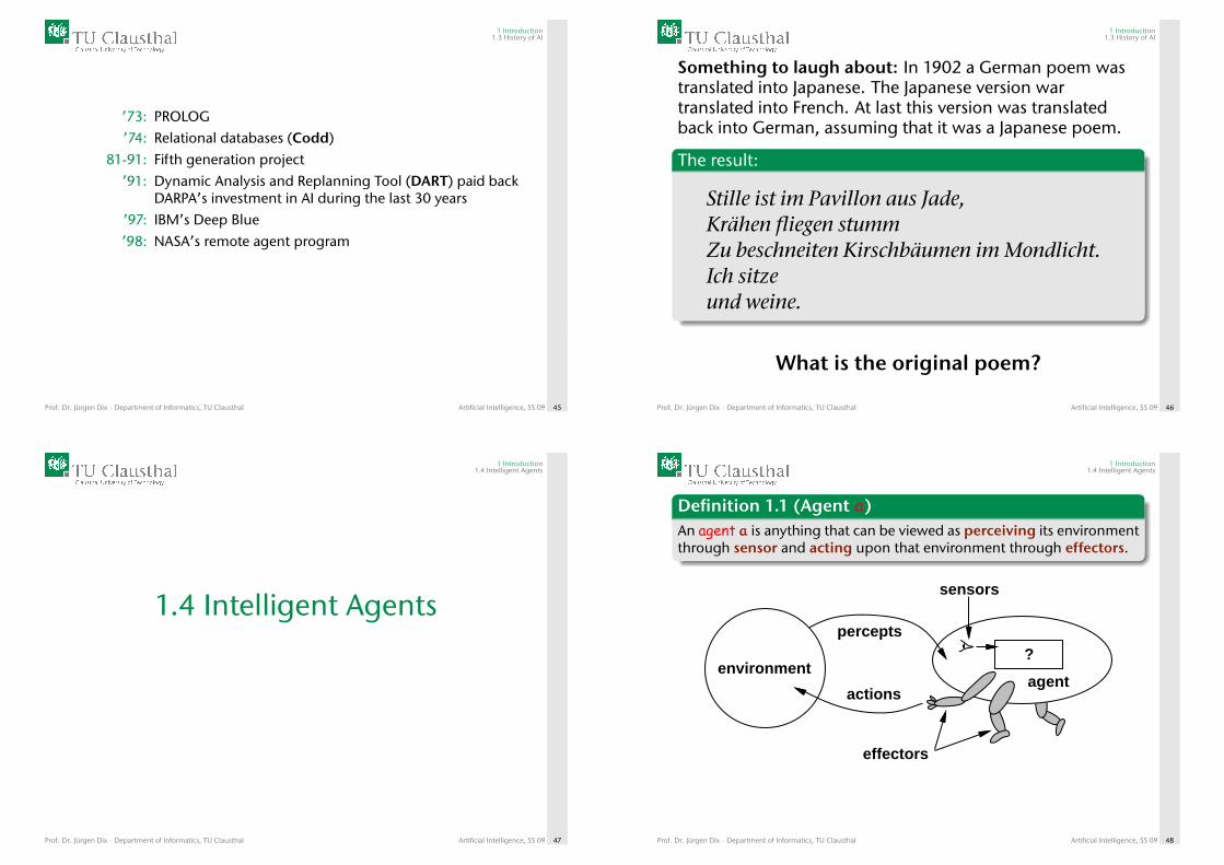
’73: PROLOG’74: Relational databases (Codd)
81-91: Fifth generation project’91: Dynamic Analysis and Replanning Tool (DART) paid back
DARPA’s investment in AI during the last 30 years’97: IBM’s Deep Blue’98: NASA’s remote agent program
Prof. Dr. Jürgen Dix · Department of Informatics, TU Clausthal Artificial Intelligence, SS 09 45
1 Introduction1.3 History of AI
Something to laugh about: In 1902 a German poem wastranslated into Japanese. The Japanese version wartranslated into French. At last this version was translatedback into German, assuming that it was a Japanese poem.
The result:
Stille ist im Pavillon aus Jade,Krähen fliegen stummZu beschneiten Kirschbäumen im Mondlicht.Ich sitzeund weine.
What is the original poem?
Prof. Dr. Jürgen Dix · Department of Informatics, TU Clausthal Artificial Intelligence, SS 09 46
1 Introduction1.4 Intelligent Agents
1.4 Intelligent Agents
Prof. Dr. Jürgen Dix · Department of Informatics, TU Clausthal Artificial Intelligence, SS 09 47
1 Introduction1.4 Intelligent Agents
Definition 1.1 (Agent aaa)An agent aaa is anything that can be viewed as perceiving its environmentthrough sensor and acting upon that environment through effectors.
?
agent
percepts
sensors
actions
effectors
environment
Prof. Dr. Jürgen Dix · Department of Informatics, TU Clausthal Artificial Intelligence, SS 09 48
1 Introduction1.4 Intelligent Agents
Definition 1.2 (Rational Agent, Omniscient Agent)A rational agent is one that does the right thing (Performancemeasure determines how successful an agent is).
A omniscient agent knows the actual outcome of his actions and can actaccordingly.
Attention:
A rational agent is in general not omniscient!
Prof. Dr. Jürgen Dix · Department of Informatics, TU Clausthal Artificial Intelligence, SS 09 49
1 Introduction1.4 Intelligent Agents
QuestionWhat is the right thing and what does it depend on?
1 Performance measure (as objective as possible).2 Percept sequence (everything the agent has received so
far).3 The agent’s knowledge about the environment.4 How the agent can act.
Prof. Dr. Jürgen Dix · Department of Informatics, TU Clausthal Artificial Intelligence, SS 09 50
1 Introduction1.4 Intelligent Agents
Definition 1.3 (Ideal Rational Agent)For each possible percept-sequence an ideal rational agent should dowhatever action is expected to maximize its performance measure(based on the evidence provided by the percepts and built-inknowledge).
Prof. Dr. Jürgen Dix · Department of Informatics, TU Clausthal Artificial Intelligence, SS 09 51
1 Introduction1.4 Intelligent Agents
Mappings:
set of percept sequences 7→ set of actions
can be used to describe agents in a mathematical way.
Hint:Internally an agent is
agent = architecture + program
AI is engaged in designing agent programs
Prof. Dr. Jürgen Dix · Department of Informatics, TU Clausthal Artificial Intelligence, SS 09 52
1 Introduction1.4 Intelligent Agents
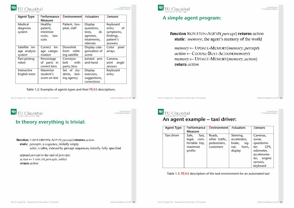
Agent Type PerformanceMeasure
Environment Actuators Sensors
Medicaldiagnosissystem
Healthypatient,minimizecosts, law-suits
Patient, hos-pital, staff
Displayquestions,tests, di-agnoses,treatments,referrals
Keyboardentry ofsymptoms,findings,patient’sanswers
Satellite im-age analysissystem
Correct im-age catego-rization
Downlinkfrom orbit-ing satellite
Display cate-gorization ofscene
Color pixelarrays
Part-pickingrobot
Percentageof parts incorrect bins
Conveyorbelt withparts; bins
Jointed armand hand
Camera,joint anglesensors
InteractiveEnglish tutor
Maximizestudent’sscore on test
Set of stu-dents, test-ing agency
Displayexercises,suggestions,corrections
Keyboardentry
Table 1.2: Examples of agents types and their PEAS descriptions.
Prof. Dr. Jürgen Dix · Department of Informatics, TU Clausthal Artificial Intelligence, SS 09 53
1 Introduction1.4 Intelligent Agents
A simple agent program:
Prof. Dr. Jürgen Dix · Department of Informatics, TU Clausthal Artificial Intelligence, SS 09 54
1 Introduction1.4 Intelligent Agents
In theory everything is trivial:
Prof. Dr. Jürgen Dix · Department of Informatics, TU Clausthal Artificial Intelligence, SS 09 55
1 Introduction1.4 Intelligent Agents
An agent example – taxi driver:
Agent Type PerformanceMeasure
Environment Actuators Sensors
Taxi driver Safe, fast,legal, com-fortable trip,maximizeprofits
Roads,other traffic,pedestrians,customers
Steering,accelerator,brake, sig-nal, horn,display
Cameras,sonar,speedome-ter, GPS,odometer,accelerome-ter, enginesensors,keyboard
Table 1.3: PEAS description of the task environment for an automated taxi
Prof. Dr. Jürgen Dix · Department of Informatics, TU Clausthal Artificial Intelligence, SS 09 56
1 Introduction1.4 Intelligent Agents
Some examples:
1 Production rules: If the driver in front hits the breaks, then hit thebreaks too.
Prof. Dr. Jürgen Dix · Department of Informatics, TU Clausthal Artificial Intelligence, SS 09 57
1 Introduction1.4 Intelligent Agents
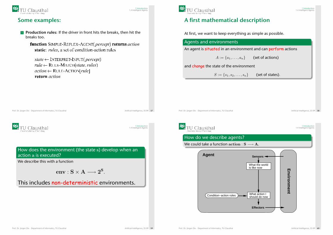
A first mathematical description
At first, we want to keep everything as simple as possible.
Agents and environmentsAn agent is situated in an environment and can perform actions
A := {a1, . . . , an} (set of actions)
and change the state of the environment
S := {s1, s2, . . . , sn} (set of states).
Prof. Dr. Jürgen Dix · Department of Informatics, TU Clausthal Artificial Intelligence, SS 09 58
1 Introduction1.4 Intelligent Agents
How does the environment (the state s) develop when anaction a is executed?We describe this with a function
env : S×A −→ 2S.
This includes non-deterministic environments.
Prof. Dr. Jürgen Dix · Department of Informatics, TU Clausthal Artificial Intelligence, SS 09 59
1 Introduction1.4 Intelligent Agents
How do we describe agents?We could take a function action : S −→ A.
Agent
En
viron
men
t
Sensors
Effectors
What the worldis like now
What action Ishould do nowCondition−action rules
Prof. Dr. Jürgen Dix · Department of Informatics, TU Clausthal Artificial Intelligence, SS 09 60
1 Introduction1.4 Intelligent Agents
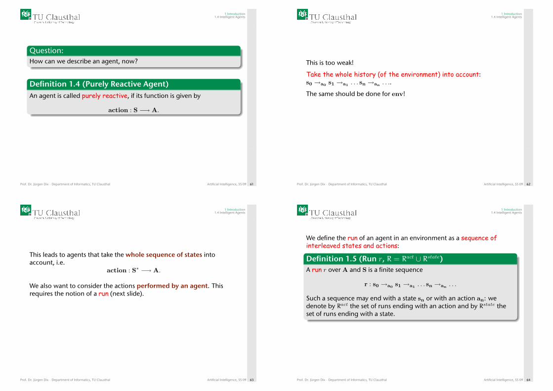
Question:How can we describe an agent, now?
Definition 1.4 (Purely Reactive Agent)An agent is called purely reactive, if its function is given by
action : S −→ A.
Prof. Dr. Jürgen Dix · Department of Informatics, TU Clausthal Artificial Intelligence, SS 09 61
1 Introduction1.4 Intelligent Agents
This is too weak!
Take the whole history (of the environment) into account:s0 →a0 s1 →a1 . . . sn →an . . ..
The same should be done for env!
Prof. Dr. Jürgen Dix · Department of Informatics, TU Clausthal Artificial Intelligence, SS 09 62
1 Introduction1.4 Intelligent Agents
This leads to agents that take the whole sequence of states intoaccount, i.e.
action : S∗ −→ A.
We also want to consider the actions performed by an agent. Thisrequires the notion of a run (next slide).
Prof. Dr. Jürgen Dix · Department of Informatics, TU Clausthal Artificial Intelligence, SS 09 63
1 Introduction1.4 Intelligent Agents
We define the run of an agent in an environment as a sequence ofinterleaved states and actions:
Definition 1.5 (Run r, R = Ract ∪ Rstate)A run r over A and S is a finite sequence
r : s0 →a0 s1 →a1 . . . sn →an . . .
Such a sequence may end with a state sn or with an action an: wedenote by Ract the set of runs ending with an action and by Rstate theset of runs ending with a state.
Prof. Dr. Jürgen Dix · Department of Informatics, TU Clausthal Artificial Intelligence, SS 09 64
1 Introduction1.4 Intelligent Agents
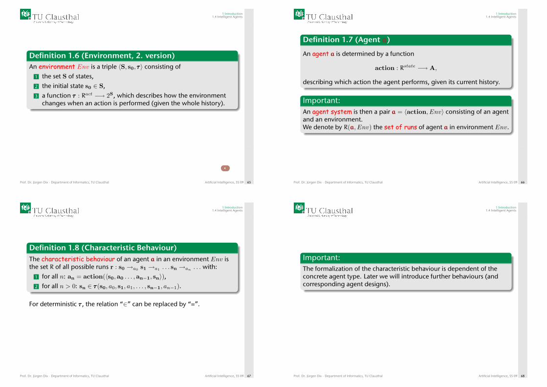
Definition 1.6 (Environment, 2. version)An environment Env is a triple 〈S, s0, τττ〉 consisting of
1 the set S of states,2 the initial state s0 ∈ S,3 a function τττ : Ract −→ 2S, which describes how the environment
changes when an action is performed (given the whole history).
Prof. Dr. Jürgen Dix · Department of Informatics, TU Clausthal Artificial Intelligence, SS 09 65
1 Introduction1.4 Intelligent Agents
Definition 1.7 (Agent aaa)
An agent aaa is determined by a function
action : Rstate −→ A,
describing which action the agent performs, given its current history.
Important:An agent system is then a pair aaa = 〈action, Env〉 consisting of an agentand an environment.We denote by R(aaa, Env) the set of runs of agent aaa in environment Env.
Prof. Dr. Jürgen Dix · Department of Informatics, TU Clausthal Artificial Intelligence, SS 09 66
1 Introduction1.4 Intelligent Agents
Definition 1.8 (Characteristic Behaviour)The characteristic behaviour of an agent aaa in an environment Env isthe set R of all possible runs r : s0 →a0 s1 →a1 . . . sn →an
. . . with:1 for all n: an = action(〈s0,a0 . . . ,an−1, sn〉),2 for all n > 0: sn ∈ τττ(s0, a0, s1, a1, . . . , sn−1, an−1).
For deterministic τττ , the relation “∈” can be replaced by “=”.
Prof. Dr. Jürgen Dix · Department of Informatics, TU Clausthal Artificial Intelligence, SS 09 67
1 Introduction1.4 Intelligent Agents
Important:The formalization of the characteristic behaviour is dependent of theconcrete agent type. Later we will introduce further behaviours (andcorresponding agent designs).
Prof. Dr. Jürgen Dix · Department of Informatics, TU Clausthal Artificial Intelligence, SS 09 68
1 Introduction1.4 Intelligent Agents
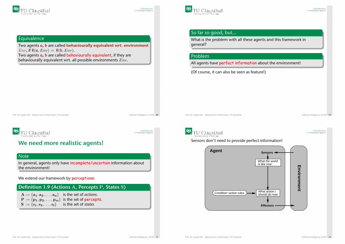
EquivalenceTwo agents aaa, bbb are called behaviourally equivalent wrt. environmentEnv, if R(aaa, Env) = R(bbb, Env).Two agents aaa, bbb are called behaviourally equivalent, if they arebehaviourally equivalent wrt. all possible environments Env.
Prof. Dr. Jürgen Dix · Department of Informatics, TU Clausthal Artificial Intelligence, SS 09 69
1 Introduction1.4 Intelligent Agents
So far so good, but...What is the problem with all these agents and this framework ingeneral?
ProblemAll agents have perfect information about the environment!
(Of course, it can also be seen as feature!)
Prof. Dr. Jürgen Dix · Department of Informatics, TU Clausthal Artificial Intelligence, SS 09 70
1 Introduction1.4 Intelligent Agents
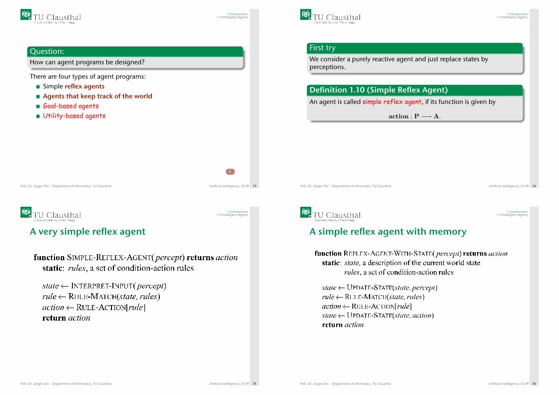
We need more realistic agents!
NoteIn general, agents only have incomplete/uncertain information aboutthe environment!
We extend our framework by perceptions:
Definition 1.9 (Actions A, Percepts P, States S)A := {a1,a2, . . . ,an} is the set of actions.P := {p1,p2, . . . ,pm} is the set of percepts.S := {s1, s2, . . . , sl} is the set of states
Prof. Dr. Jürgen Dix · Department of Informatics, TU Clausthal Artificial Intelligence, SS 09 71
1 Introduction1.4 Intelligent Agents
Sensors don’t need to provide perfect information!
Agent
En
viron
men
t
Sensors
Effectors
What the worldis like now
What action Ishould do nowCondition−action rules
Prof. Dr. Jürgen Dix · Department of Informatics, TU Clausthal Artificial Intelligence, SS 09 72
1 Introduction1.4 Intelligent Agents
Question:How can agent programs be designed?
There are four types of agent programs:Simple reflex agentsAgents that keep track of the worldGoal-based agentsUtility-based agents
Prof. Dr. Jürgen Dix · Department of Informatics, TU Clausthal Artificial Intelligence, SS 09 73
1 Introduction1.4 Intelligent Agents
First tryWe consider a purely reactive agent and just replace states byperceptions.
Definition 1.10 (Simple Reflex Agent)An agent is called simple reflex agent, if its function is given by
action : P −→ A.
Prof. Dr. Jürgen Dix · Department of Informatics, TU Clausthal Artificial Intelligence, SS 09 74
1 Introduction1.4 Intelligent Agents
A very simple reflex agent
Prof. Dr. Jürgen Dix · Department of Informatics, TU Clausthal Artificial Intelligence, SS 09 75
1 Introduction1.4 Intelligent Agents
A simple reflex agent with memory
Prof. Dr. Jürgen Dix · Department of Informatics, TU Clausthal Artificial Intelligence, SS 09 76
1 Introduction1.4 Intelligent Agents
As before, let us now consider sequences of percepts:
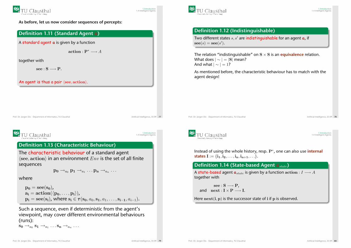
Definition 1.11 (Standard Agent aaa)
A standard agent aaa is given by a function
action : P∗ −→ A
together with
see : S −→ P.
An agent is thus a pair 〈see,action〉.
Prof. Dr. Jürgen Dix · Department of Informatics, TU Clausthal Artificial Intelligence, SS 09 77
1 Introduction1.4 Intelligent Agents
Definition 1.12 (Indistinguishable)Two different states s, s′ are indistinguishable for an agent aaa, ifsee(s) = see(s′).
The relation “indistinguishable” on S× S is an equivalence relation.What does | ∼ | = |S|mean?And what | ∼ | = 1?
As mentioned before, the characteristic behaviour has to match with theagent design!
Prof. Dr. Jürgen Dix · Department of Informatics, TU Clausthal Artificial Intelligence, SS 09 78
1 Introduction1.4 Intelligent Agents
Definition 1.13 (Characteristic Behaviour)
The characteristic behaviour of a standard agent〈see, action〉 in an environment Env is the set of all finitesequences
p0 →a0 p1 →a1 . . .pn →an . . .
where
p0 = see(s0),ai = action(〈p0, . . . ,pi〉),pi = see(si), where si ∈ τττ(s0, a0, s1, a1, . . . , si−1, ai−1).
Such a sequence, even if deterministic from the agent’sviewpoint, may cover different environmental behaviours(runs):s0 →a0 s1 →a1 . . . sn →an . . .
Prof. Dr. Jürgen Dix · Department of Informatics, TU Clausthal Artificial Intelligence, SS 09 79
1 Introduction1.4 Intelligent Agents
Instead of using the whole history, resp. P∗, one can also use internalstates I := {i1, i2, . . . , in, in+1, . . .}.
Definition 1.14 (State-based Agent aaastate)A state-based agent aaastate is given by a function action : I −→ Atogether with
see : S −→ P,and next : I×P −→ I.
Here next(i,p) is the successor state of i if p is observed.
Prof. Dr. Jürgen Dix · Department of Informatics, TU Clausthal Artificial Intelligence, SS 09 80
1 Introduction1.4 Intelligent Agents
Agent
En
viron
men
t
Sensors
Effectors
What the worldis like now
What action Ishould do now
State
How the world evolves
What my actions do
Condition−action rules
Prof. Dr. Jürgen Dix · Department of Informatics, TU Clausthal Artificial Intelligence, SS 09 81
1 Introduction1.4 Intelligent Agents
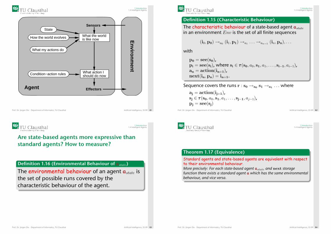
Definition 1.15 (Characteristic Behaviour)
The characteristic behaviour of a state-based agent aaastatein an environment Env is the set of all finite sequences
(i0,p0)→a0 (i1,p1)→a1 . . .→an−1 (in,pn), . . .
with
p0 = see(s0),pi = see(si), where si ∈ τττ(s0, a0, s1, a1, . . . , si−1, ai−1),an = action(in+1),next(in,pn) = in+1.
Sequence covers the runs r : s0 →a0 s1 →a1 . . . whereaj = action(ij+1),sj ∈ τττ(s0, a0, s1, a1, . . . , sj−1, aj−1),pj = see(sj)
Prof. Dr. Jürgen Dix · Department of Informatics, TU Clausthal Artificial Intelligence, SS 09 82
1 Introduction1.4 Intelligent Agents
Are state-based agents more expressive thanstandard agents? How to measure?
Definition 1.16 (Environmental Behaviour of aaastate)
The environmental behaviour of an agent aaastate isthe set of possible runs covered by thecharacteristic behaviour of the agent.
Prof. Dr. Jürgen Dix · Department of Informatics, TU Clausthal Artificial Intelligence, SS 09 83
1 Introduction1.4 Intelligent Agents
Theorem 1.17 (Equivalence)Standard agents and state-based agents are equivalent with respectto their environmental behaviour.More precisely: For each state-based agent aaastate and next storagefunction there exists a standard agent aaa which has the same environmentalbehaviour, and vice versa.
Prof. Dr. Jürgen Dix · Department of Informatics, TU Clausthal Artificial Intelligence, SS 09 84
1 Introduction1.4 Intelligent Agents
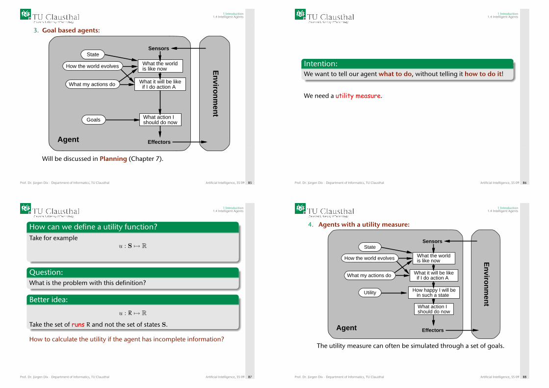
3. Goal based agents:
Agent
En
viron
men
t
Sensors
Effectors
What it will be like if I do action A
What the worldis like now
What action Ishould do now
State
How the world evolves
What my actions do
Goals
Will be discussed in Planning (Chapter 7).
Prof. Dr. Jürgen Dix · Department of Informatics, TU Clausthal Artificial Intelligence, SS 09 85
1 Introduction1.4 Intelligent Agents
Intention:We want to tell our agent what to do, without telling it how to do it!
We need a utility measure.
Prof. Dr. Jürgen Dix · Department of Informatics, TU Clausthal Artificial Intelligence, SS 09 86
1 Introduction1.4 Intelligent Agents
How can we define a utility function?Take for example
u : S 7→ R
Question:What is the problem with this definition?
Better idea:
u : R 7→ R
Take the set of runs R and not the set of states S.
How to calculate the utility if the agent has incomplete information?
Prof. Dr. Jürgen Dix · Department of Informatics, TU Clausthal Artificial Intelligence, SS 09 87
1 Introduction1.4 Intelligent Agents
4. Agents with a utility measure:
Agent
En
viron
men
t
Sensors
Effectors
What it will be like if I do action A
What the worldis like now
How happy I will be in such a state
What action Ishould do now
State
How the world evolves
What my actions do
Utility
The utility measure can often be simulated through a set of goals.
Prof. Dr. Jürgen Dix · Department of Informatics, TU Clausthal Artificial Intelligence, SS 09 88
1 Introduction1.4 Intelligent Agents
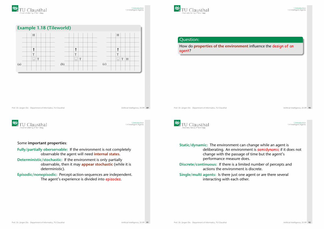
Example 1.18 (Tileworld)H
H
H
T T T
T T T
(a) (b) (c)
Prof. Dr. Jürgen Dix · Department of Informatics, TU Clausthal Artificial Intelligence, SS 09 89
1 Introduction1.4 Intelligent Agents
Question:How do properties of the environment influence the design of anagent?
Prof. Dr. Jürgen Dix · Department of Informatics, TU Clausthal Artificial Intelligence, SS 09 90
1 Introduction1.4 Intelligent Agents
Some important properties:
Fully/partially oberservable: If the environment is not completelyobservable the agent will need internal states.
Deterministic/stochastic: If the environment is only partiallyobservable, then it may appear stochastic (while it isdeterministic).
Episodic/nonepisodic: Percept-action-sequences are independent.The agent’s experience is divided into episodes.
Prof. Dr. Jürgen Dix · Department of Informatics, TU Clausthal Artificial Intelligence, SS 09 91
1 Introduction1.4 Intelligent Agents
Static/dynamic: The environment can change while an agent isdeliberating. An environment is semidynamic if it does notchange with the passage of time but the agent’sperformance measure does.
Discrete/continuous: If there is a limited number of percepts andactions the environment is discrete.
Single/multi agents: Is there just one agent or are there severalinteracting with each other.
Prof. Dr. Jürgen Dix · Department of Informatics, TU Clausthal Artificial Intelligence, SS 09 92
1 Introduction1.4 Intelligent Agents
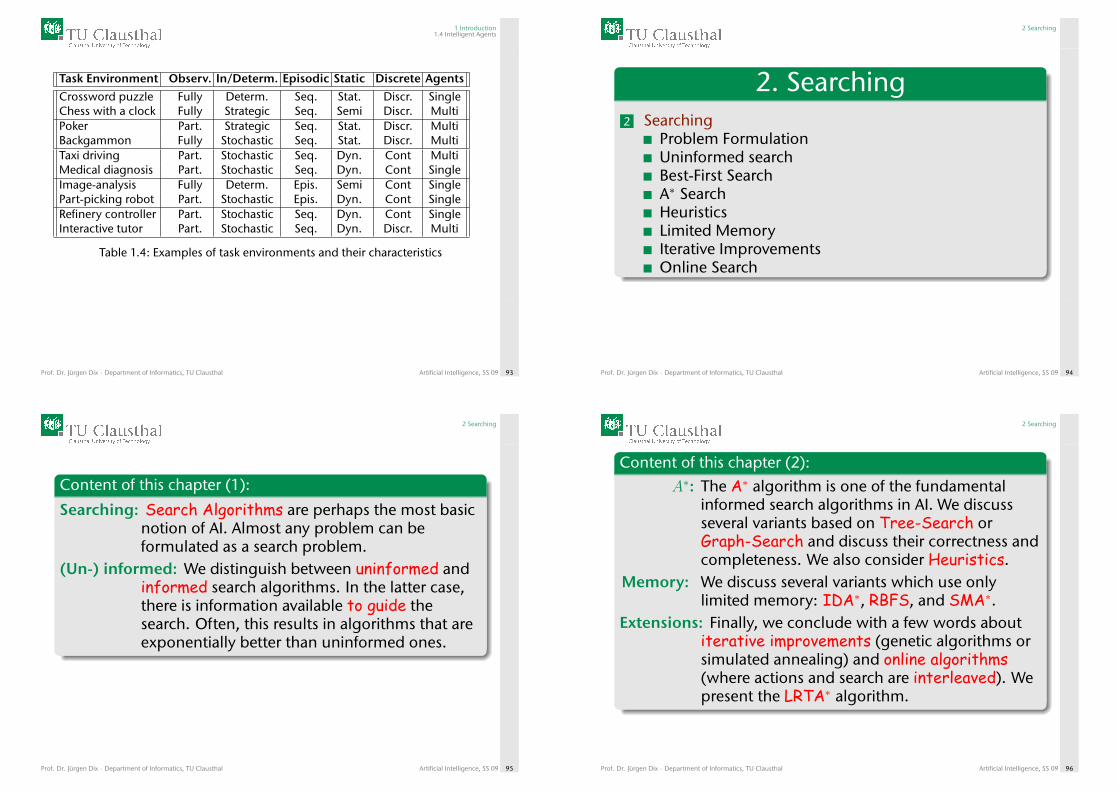
Task Environment Observ. In/Determ. Episodic Static Discrete Agents
Crossword puzzle Fully Determ. Seq. Stat. Discr. SingleChess with a clock Fully Strategic Seq. Semi Discr. MultiPoker Part. Strategic Seq. Stat. Discr. MultiBackgammon Fully Stochastic Seq. Stat. Discr. MultiTaxi driving Part. Stochastic Seq. Dyn. Cont MultiMedical diagnosis Part. Stochastic Seq. Dyn. Cont SingleImage-analysis Fully Determ. Epis. Semi Cont SinglePart-picking robot Part. Stochastic Epis. Dyn. Cont SingleRefinery controller Part. Stochastic Seq. Dyn. Cont SingleInteractive tutor Part. Stochastic Seq. Dyn. Discr. Multi
Table 1.4: Examples of task environments and their characteristics
Prof. Dr. Jürgen Dix · Department of Informatics, TU Clausthal Artificial Intelligence, SS 09 93
2 Searching
2. Searching2 Searching
Problem FormulationUninformed searchBest-First SearchA∗ SearchHeuristicsLimited MemoryIterative ImprovementsOnline Search
Prof. Dr. Jürgen Dix · Department of Informatics, TU Clausthal Artificial Intelligence, SS 09 94
2 Searching
Content of this chapter (1):
Searching: Search Algorithms are perhaps the most basicnotion of AI. Almost any problem can beformulated as a search problem.
(Un-) informed: We distinguish between uninformed andinformed search algorithms. In the latter case,there is information available to guide thesearch. Often, this results in algorithms that areexponentially better than uninformed ones.
Prof. Dr. Jürgen Dix · Department of Informatics, TU Clausthal Artificial Intelligence, SS 09 95
2 Searching
Content of this chapter (2):
A∗: The A∗ algorithm is one of the fundamentalinformed search algorithms in AI. We discussseveral variants based on Tree-Search orGraph-Search and discuss their correctness andcompleteness. We also consider Heuristics.
Memory: We discuss several variants which use onlylimited memory: IDA∗, RBFS, and SMA∗.
Extensions: Finally, we conclude with a few words aboutiterative improvements (genetic algorithms orsimulated annealing) and online algorithms(where actions and search are interleaved). Wepresent the LRTA∗ algorithm.
Prof. Dr. Jürgen Dix · Department of Informatics, TU Clausthal Artificial Intelligence, SS 09 96
2 Searching
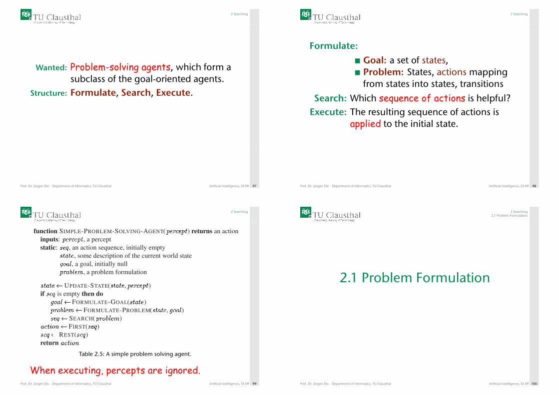
Wanted: Problem-solving agents, which form asubclass of the goal-oriented agents.
Structure: Formulate, Search, Execute.
Prof. Dr. Jürgen Dix · Department of Informatics, TU Clausthal Artificial Intelligence, SS 09 97
2 Searching
Formulate:
Goal: a set of states,Problem: States, actions mappingfrom states into states, transitions
Search: Which sequence of actions is helpful?Execute: The resulting sequence of actions is
applied to the initial state.
Prof. Dr. Jürgen Dix · Department of Informatics, TU Clausthal Artificial Intelligence, SS 09 98
2 Searching
function SIMPLE-PROBLEM-SOLVING-AGENT( � � � � � � ) returns an actioninputs: � � � � � � , a perceptstatic: � � � , an action sequence, initially empty
� � � , some description of the current world state� � � � , a goal, initially null
� � � � � � � , a problem formulation
� � � � UPDATE-STATE( � � � , � � � � � � )if � � � is empty then do
� � � � � FORMULATE-GOAL( � � � )� � � � � � � � FORMULATE-PROBLEM( � � � , � � � � )
� � � � SEARCH( � � � � � � � )� � % � & � FIRST( � � � )
� � � � REST( � � � )return � � % � &
Table 2.5: A simple problem solving agent.
When executing, percepts are ignored.Prof. Dr. Jürgen Dix · Department of Informatics, TU Clausthal Artificial Intelligence, SS 09 99
2 Searching2.1 Problem Formulation
2.1 Problem Formulation
Prof. Dr. Jürgen Dix · Department of Informatics, TU Clausthal Artificial Intelligence, SS 09 100
2 Searching2.1 Problem Formulation
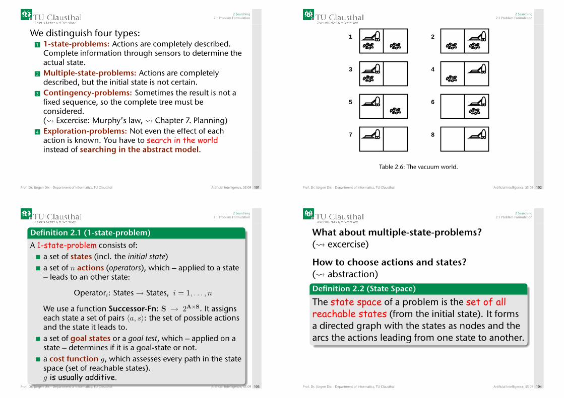
We distinguish four types:1 1-state-problems: Actions are completely described.
Complete information through sensors to determine theactual state.
2 Multiple-state-problems: Actions are completelydescribed, but the initial state is not certain.
3 Contingency-problems: Sometimes the result is not afixed sequence, so the complete tree must beconsidered.( Excercise: Murphy’s law, Chapter 7. Planning)
4 Exploration-problems: Not even the effect of eachaction is known. You have to search in the worldinstead of searching in the abstract model.
Prof. Dr. Jürgen Dix · Department of Informatics, TU Clausthal Artificial Intelligence, SS 09 101
2 Searching2.1 Problem Formulation
1 2
3 4
5 6
7 8
Table 2.6: The vacuum world.
Prof. Dr. Jürgen Dix · Department of Informatics, TU Clausthal Artificial Intelligence, SS 09 102
2 Searching2.1 Problem Formulation
Definition 2.1 (1-state-problem)
A 1-state-problem consists of:a set of states (incl. the initial state)a set of n actions (operators), which – applied to a state– leads to an other state:
Operatori: States→ States, i = 1, . . . , n
We use a function Successor-Fn: S → 2A×S. It assignseach state a set of pairs 〈a, s〉: the set of possible actionsand the state it leads to.a set of goal states or a goal test, which – applied on astate – determines if it is a goal-state or not.a cost function g, which assesses every path in the statespace (set of reachable states).g is usually additive.
Prof. Dr. Jürgen Dix · Department of Informatics, TU Clausthal Artificial Intelligence, SS 09 103
2 Searching2.1 Problem Formulation
What about multiple-state-problems?( excercise)
How to choose actions and states?( abstraction)Definition 2.2 (State Space)
The state space of a problem is the set of allreachable states (from the initial state). It formsa directed graph with the states as nodes and thearcs the actions leading from one state to another.
Prof. Dr. Jürgen Dix · Department of Informatics, TU Clausthal Artificial Intelligence, SS 09 104
2 Searching2.1 Problem Formulation
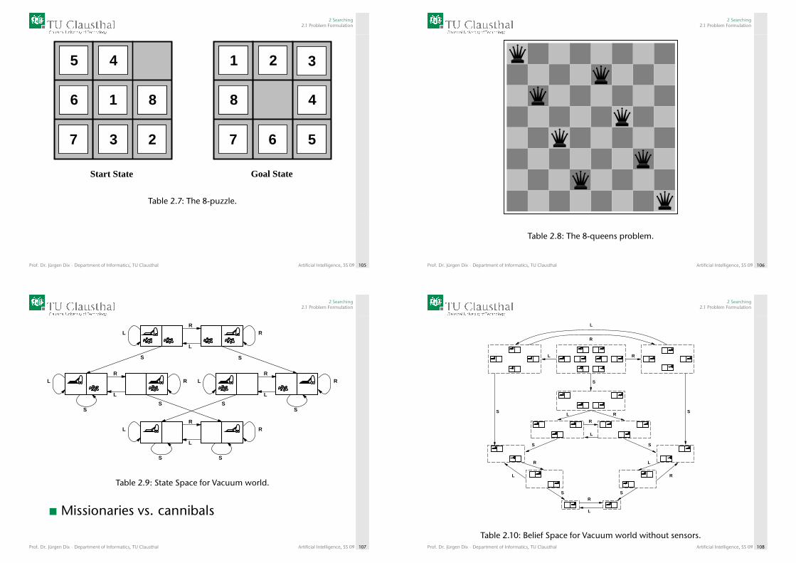
Start State Goal State
2
45
6
7
8
1 2 3
4
67
81
23
45
6
7
81
23
45
6
7
8
5
Table 2.7: The 8-puzzle.
Prof. Dr. Jürgen Dix · Department of Informatics, TU Clausthal Artificial Intelligence, SS 09 105
2 Searching2.1 Problem Formulation
Table 2.8: The 8-queens problem.
Prof. Dr. Jürgen Dix · Department of Informatics, TU Clausthal Artificial Intelligence, SS 09 106
2 Searching2.1 Problem Formulation
R
L
S S
S S
R
L
R
L
R
L
S
SS
S
L
L
LL R
R
R
R
Table 2.9: State Space for Vacuum world.
Missionaries vs. cannibals
Prof. Dr. Jürgen Dix · Department of Informatics, TU Clausthal Artificial Intelligence, SS 09 107
2 Searching2.1 Problem Formulation
L
R
L R
S
L RS S
S S
R
L
S S
L
R
R
L
R
L
Table 2.10: Belief Space for Vacuum world without sensors.Prof. Dr. Jürgen Dix · Department of Informatics, TU Clausthal Artificial Intelligence, SS 09 108
2 Searching2.1 Problem Formulation
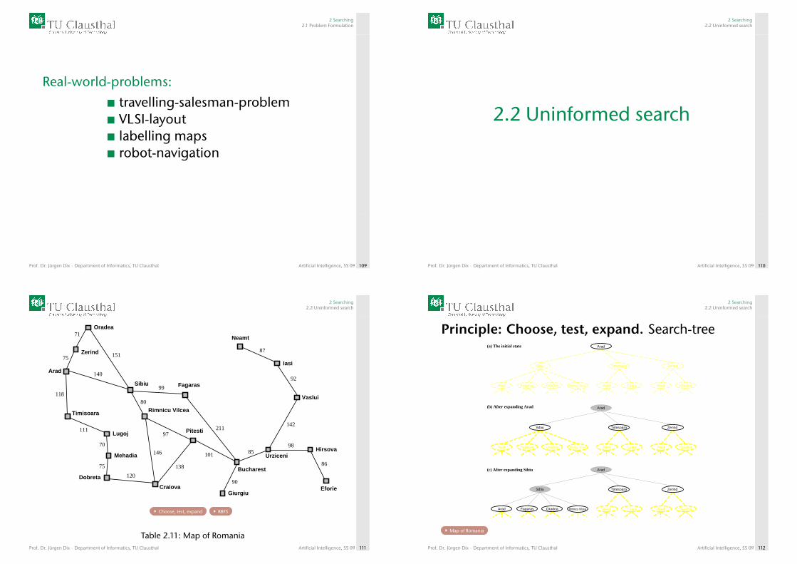
Real-world-problems:
travelling-salesman-problemVLSI-layoutlabelling mapsrobot-navigation
Prof. Dr. Jürgen Dix · Department of Informatics, TU Clausthal Artificial Intelligence, SS 09 109
2 Searching2.2 Uninformed search
2.2 Uninformed search
Prof. Dr. Jürgen Dix · Department of Informatics, TU Clausthal Artificial Intelligence, SS 09 110
2 Searching2.2 Uninformed search
Giurgiu
UrziceniHirsova
Eforie
Neamt
Oradea
Zerind
Arad
Timisoara
Lugoj
Mehadia
Dobreta
Craiova
Sibiu Fagaras
Pitesti
Vaslui
Iasi
Rimnicu Vilcea
Bucharest
71
75
118
111
70
75
120
151
140
99
80
97
101
211
138
146 85
90
98
142
92
87
86
Choose, test, expand RBFS
Table 2.11: Map of RomaniaProf. Dr. Jürgen Dix · Department of Informatics, TU Clausthal Artificial Intelligence, SS 09 111
2 Searching2.2 Uninformed search
Principle: Choose, test, expand. Search-tree(a) The initial state
(b) After expanding Arad
(c) After expanding Sibiu
Rimnicu Vilcea LugojArad Fagaras Oradea AradArad Oradea
Rimnicu Vilcea Lugoj
ZerindSibiu
Arad Fagaras Oradea
Timisoara
AradArad Oradea
Lugoj AradArad Oradea
Zerind
Arad
Sibiu Timisoara
Arad
Rimnicu Vilcea
Zerind
Arad
Sibiu
Arad Fagaras Oradea
Timisoara
Map of Romania
Prof. Dr. Jürgen Dix · Department of Informatics, TU Clausthal Artificial Intelligence, SS 09 112
2 Searching2.2 Uninformed search
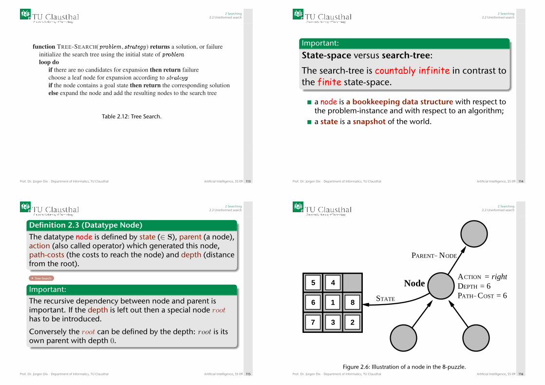
function TREE-SEARCH( � � � � � � , � � � � � � � ) returns a solution, or failureinitialize the search tree using the initial state of � � � � � �
loop doif there are no candidates for expansion then return failurechoose a leaf node for expansion according to � � � � � � �
if the node contains a goal state then return the corresponding solutionelse expand the node and add the resulting nodes to the search tree
Table 2.12: Tree Search.
Prof. Dr. Jürgen Dix · Department of Informatics, TU Clausthal Artificial Intelligence, SS 09 113
2 Searching2.2 Uninformed search
Important:
State-space versus search-tree:
The search-tree is countably infinite in contrast tothe finite state-space.
a node is a bookkeeping data structure with respect tothe problem-instance and with respect to an algorithm;a state is a snapshot of the world.
Prof. Dr. Jürgen Dix · Department of Informatics, TU Clausthal Artificial Intelligence, SS 09 114
2 Searching2.2 Uninformed search
Definition 2.3 (Datatype Node)
The datatype node is defined by state (∈ S), parent (a node),action (also called operator) which generated this node,path-costs (the costs to reach the node) and depth (distancefrom the root).
Tree-Search
Important:
The recursive dependency between node and parent isimportant. If the depth is left out then a special node roothas to be introduced.
Conversely the root can be defined by the depth: root is itsown parent with depth 0.
Prof. Dr. Jürgen Dix · Department of Informatics, TU Clausthal Artificial Intelligence, SS 09 115
2 Searching2.2 Uninformed search
1
23
45
6
7
81
23
45
6
7
8
Node
PARENT− NODE
STATE P COSTATH− = 6DEPTH = 6ACTION = right
Figure 2.6: Illustration of a node in the 8-puzzle.Prof. Dr. Jürgen Dix · Department of Informatics, TU Clausthal Artificial Intelligence, SS 09 116

2 Searching2.2 Uninformed search
Now we will try to instantiate the functionTree-SEARCH a bit.
Design-decision: QueueThe nodes-to-be-expanded can be described as aset. But we will use a queue instead.The fringe is the set of generated nodes that arenot yet expanded.
Here are a few functions operating on queues:Make-Queue(Elements) Remove-First(Queue)Empty?(Queue) Insert(Element,Queue)First(Queue) Insert-All(Elements,Queue)
Prof. Dr. Jürgen Dix · Department of Informatics, TU Clausthal Artificial Intelligence, SS 09 117
2 Searching2.2 Uninformed search
function TREE-SEARCH( � � � � � � � � � � � � ) returns a solution, or failure
� � � � INSERT(MAKE-NODE(INITIAL-STATE[ � � � � � � � ]), � � � � )loop do
if EMPTY?( � � � � ) then return failure� � � � REMOVE-FIRST( � � � � )if GOAL-TEST[ � � � � � � � ] applied to STATE[ � � � � ] succeeds
then return SOLUTION( � � � � ) � � � � INSERT-ALL(EXPAND( � � � � , � � � � � � � ), � � � � )
function EXPAND( � � � � � � � � � � � � ) returns a set of nodes
� � � � � � � � � � the empty setfor each � � � � � � , � � � � � � � in SUCCESSOR-FN[ � � � � � � � ](STATE[ � � � � ]) do
� a new NODE
STATE[ � ] � � � � � �PARENT-NODE[ � ] � � � �ACTION[ � ] � � � � �PATH-COST[ � ] PATH-COST[ � � � � ] + STEP-COST( � � � � , � � � � � , � )DEPTH[ � ] DEPTH[ � � � � ] + 1add � to � � � � � � � � � �
return � � � � � � � � � �
Datatype Node
Graph-Search
Table 2.13: Tree-Search
Prof. Dr. Jürgen Dix · Department of Informatics, TU Clausthal Artificial Intelligence, SS 09 118
2 Searching2.2 Uninformed search
Question:
Which are interesting requirements ofsearch-strategies?
completenesstime-complexityspace complexityoptimality (w.r.t. path-costs)
We distinguish:
Uninformed vs. informed search.
Prof. Dr. Jürgen Dix · Department of Informatics, TU Clausthal Artificial Intelligence, SS 09 119
2 Searching2.2 Uninformed search
Breadth-first-search: “nodes with the smallestdepth are expanded first”,
Make-Queue : add new nodes at the end: FIFOComplete? Yes.Optimal? Yes, if all operators are equally expensive.
Constant branching-factor b: for a solution atdepth d we have generated (in the worst case)
b+ b2 + . . .+ bd + (bd+1 − b)-many nodes.Space complexity = Time Complexity
Prof. Dr. Jürgen Dix · Department of Informatics, TU Clausthal Artificial Intelligence, SS 09 120
2 Searching2.2 Uninformed search
A
B C
D E F G
A
B C
D E F G
A
B C
D E F G
A
B C
D E F G
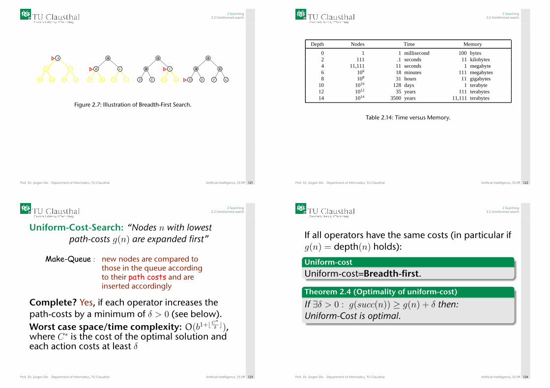
Figure 2.7: Illustration of Breadth-First Search.
Prof. Dr. Jürgen Dix · Department of Informatics, TU Clausthal Artificial Intelligence, SS 09 121
2 Searching2.2 Uninformed search
Depth Nodes Time Memory
0 1 1 millisecond 100 bytes2 111 .1 seconds 11 kilobytes4 11,111 11 seconds 1 megabyte6 106 18 minutes 111 megabytes8 108 31 hours 11 gigabytes
10 1010 128 days 1 terabyte12 1012 35 years 111 terabytes14 1014 3500 years 11,111 terabytes
Table 2.14: Time versus Memory.
Prof. Dr. Jürgen Dix · Department of Informatics, TU Clausthal Artificial Intelligence, SS 09 122
2 Searching2.2 Uninformed search
Uniform-Cost-Search: “Nodes n with lowestpath-costs g(n) are expanded first”
Make-Queue : new nodes are compared tothose in the queue accordingto their path costs and areinserted accordingly
Complete? Yes, if each operator increases thepath-costs by a minimum of δ > 0 (see below).Worst case space/time complexity: O(b1+bC
∗δ c),
where C∗ is the cost of the optimal solution andeach action costs at least δ
Prof. Dr. Jürgen Dix · Department of Informatics, TU Clausthal Artificial Intelligence, SS 09 123
2 Searching2.2 Uninformed search
If all operators have the same costs (in particular ifg(n) = depth(n) holds):
Uniform-cost
Uniform-cost=Breadth-first.
Theorem 2.4 (Optimality of uniform-cost)
If ∃δ > 0 : g(succ(n)) ≥ g(n) + δ then:Uniform-Cost is optimal.
Prof. Dr. Jürgen Dix · Department of Informatics, TU Clausthal Artificial Intelligence, SS 09 124
2 Searching2.2 Uninformed search
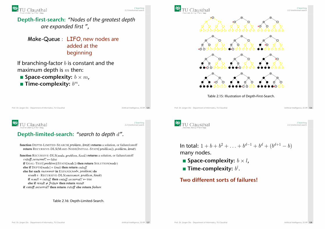
Depth-first-search: “Nodes of the greatest depthare expanded first ”,
Make-Queue : LIFO,new nodes areadded at thebeginning
If branching-factor b is constant and themaximum depth is m then:
Space-complexity: b×m,Time-complexity: bm.
Prof. Dr. Jürgen Dix · Department of Informatics, TU Clausthal Artificial Intelligence, SS 09 125
2 Searching2.2 Uninformed search
A
B C
D E F G
H I J K L M N O
A
B C
D E F G
H I J K L M N O
A
B C
D E F G
H I J K L M N O
A
B C
D E F G
H I J K L M N O
A
B C
D E F G
H I J K L M N O
A
B C
D E F G
H I J K L M N O
A
B C
D E F G
H I J K L M N O
A
B C
D E F G
H I J K L M N O
A
B C
D E F G
H I J K L M N O
A
B C
D E F G
H I J K L M N O
A
B C
D E F G
H I J K L M N O
A
B C
D E F G
H I J K L M N O
Table 2.15: Illustration of Depth-First-Search.
Prof. Dr. Jürgen Dix · Department of Informatics, TU Clausthal Artificial Intelligence, SS 09 126
2 Searching2.2 Uninformed search
Depth-limited-search: “search to depth d”.
function DEPTH-LIMITED-SEARCH( � � � � � � , � � � � � ) returns a solution, or failure/cutoffreturn RECURSIVE-DLS(MAKE-NODE(INITIAL-STATE[ � � � � � � ]), � � � � � � , � � � � � )
function RECURSIVE-DLS( � � � , � � � � � � , � � � � � ) returns a solution, or failure/cutoff� � � � � � � � � � � # % falseif GOAL-TEST[ � � � � � � ](STATE[ � � � ]) then return SOLUTION( � � � )else if DEPTH[ � � � ] = � � � � � then return � � � �
else for each ) � � � ) ) � � in EXPAND( � � � , � � � � � � ) do� ) � � � % RECURSIVE-DLS( ) � � � ) ) � � , � � � � � � , � � � � � )if � ) � � � = � � � � then � � � � � � � � � � � # % trueelse if � ) � � � -. / 0 � � � � then return � ) � � �
if � � � � � � � � � � � # then return � � � � else return / 0 � � � �
Table 2.16: Depth-Limited-Search.
Prof. Dr. Jürgen Dix · Department of Informatics, TU Clausthal Artificial Intelligence, SS 09 127
2 Searching2.2 Uninformed search
In total: 1 + b+ b2 + . . .+ bd−1 + bd + (bd+1 − b)many nodes.
Space-complexity: b× l,Time-complexity: bl.
Two different sorts of failures!
Prof. Dr. Jürgen Dix · Department of Informatics, TU Clausthal Artificial Intelligence, SS 09 128
2 Searching2.2 Uninformed search
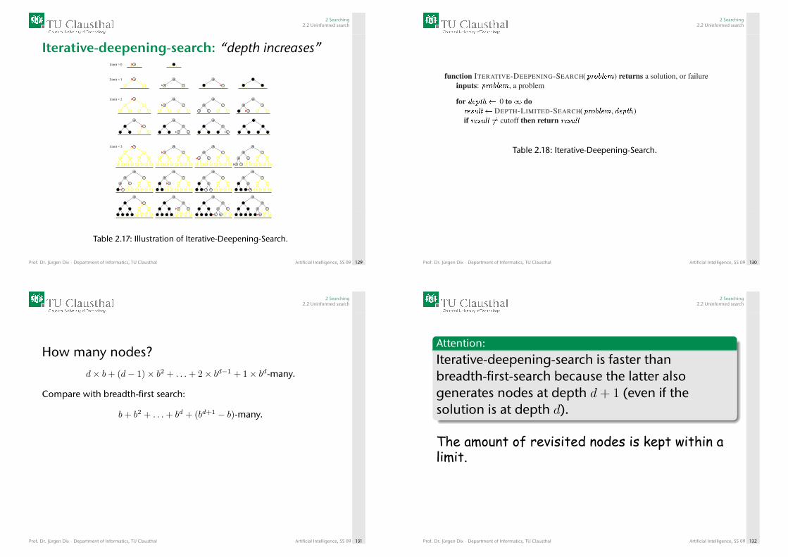
Iterative-deepening-search: “depth increases”
Limit = 3
Limit = 2
Limit = 1
Limit = 0 A A
A
B C
A
B C
A
B C
A
B C
A
B C
D E F G
A
B C
D E F G
A
B C
D E F G
A
B C
D E F G
A
B C
D E F G
A
B C
D E F G
A
B C
D E F G
A
B C
D E F G
A
B C
D E F G
H I J K L M N O
A
B C
D E F G
H I J K L M N O
A
B C
D E F G
H I J K L M N O
A
B C
D E F G
H I J K L M N O
A
B C
D E F G
H I J K L M N O
A
B C
D E F G
H I J K L M N O
A
B C
D E F G
H I J K L M N O
A
B C
D E F G
H I J K L M N O
A
B C
D E F G
H I J K L M N O
A
B C
D E F G
H I J K L M N O
A
B C
D E F G
H J K L M N OI
A
B C
D E F G
H I J K L M N O
Table 2.17: Illustration of Iterative-Deepening-Search.
Prof. Dr. Jürgen Dix · Department of Informatics, TU Clausthal Artificial Intelligence, SS 09 129
2 Searching2.2 Uninformed search
function ITERATIVE-DEEPENING-SEARCH( � � � � � � ) returns a solution, or failureinputs: � � � � � � , a problem
for � � � � � 0 to � do� � � � � � DEPTH-LIMITED-SEARCH( � � � � � � , � � � � )if � � � � � ! cutoff then return � � � � �
Table 2.18: Iterative-Deepening-Search.
Prof. Dr. Jürgen Dix · Department of Informatics, TU Clausthal Artificial Intelligence, SS 09 130
2 Searching2.2 Uninformed search
How many nodes?
d× b+ (d− 1)× b2 + . . .+ 2× bd−1 + 1× bd-many.
Compare with breadth-first search:
b+ b2 + . . .+ bd + (bd+1 − b)-many.
Prof. Dr. Jürgen Dix · Department of Informatics, TU Clausthal Artificial Intelligence, SS 09 131
2 Searching2.2 Uninformed search
Attention:
Iterative-deepening-search is faster thanbreadth-first-search because the latter alsogenerates nodes at depth d+ 1 (even if thesolution is at depth d).
The amount of revisited nodes is kept within alimit.
Prof. Dr. Jürgen Dix · Department of Informatics, TU Clausthal Artificial Intelligence, SS 09 132
2 Searching2.2 Uninformed search
GoalStart
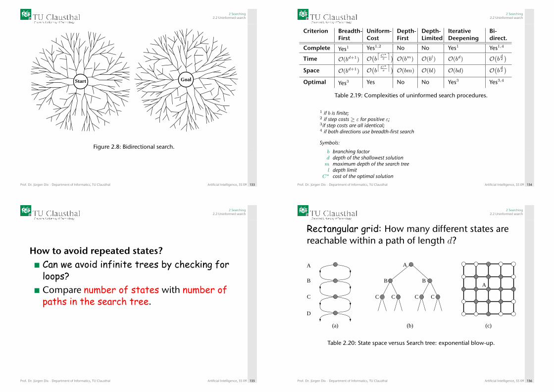
Figure 2.8: Bidirectional search.
Prof. Dr. Jürgen Dix · Department of Informatics, TU Clausthal Artificial Intelligence, SS 09 133
2 Searching2.2 Uninformed search
Criterion Breadth-First
Uniform-Cost
Depth-First
Depth-Limited
IterativeDeepening
Bi-direct.
Complete Yes1 Yes1,2 No No Yes1 Yes1,4
Time O(bd+1) O(b
⌈C∗ε
⌉)O(bm) O(bl) O(bd) O
(b
d2)
Space O(bd+1) O(b
⌈C∗ε
⌉)O(bm) O(bl) O(bd) O
(b
d2)
Optimal Yes3 Yes No No Yes3 Yes3,4
Table 2.19: Complexities of uninformed search procedures.
1 if b is finite;2 if step costs ≥ ε for positive ε;3if step costs are all identical;4 if both directions use breadth-first search
Symbols:
b branching factord depth of the shallowest solutionm maximum depth of the search treel depth limit
C∗ cost of the optimal solutionProf. Dr. Jürgen Dix · Department of Informatics, TU Clausthal Artificial Intelligence, SS 09 134
2 Searching2.2 Uninformed search
How to avoid repeated states?Can we avoid infinite trees by checking forloops?Compare number of states with number ofpaths in the search tree.
Prof. Dr. Jürgen Dix · Department of Informatics, TU Clausthal Artificial Intelligence, SS 09 135
2 Searching2.2 Uninformed search
Rectangular grid: How many different states arereachable within a path of length d?
A
B
C
D
A
B B
CC CC
A
(c)(b)(a)
Table 2.20: State space versus Search tree: exponential blow-up.
Prof. Dr. Jürgen Dix · Department of Informatics, TU Clausthal Artificial Intelligence, SS 09 136
2 Searching2.2 Uninformed search
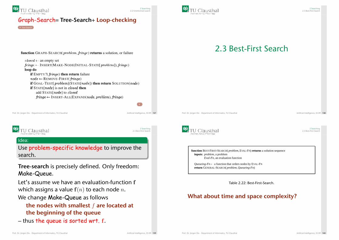
Graph-Search= Tree-Search+ Loop-checkingTree-Search
function GRAPH-SEARCH( � � � � � � � � � � � � ) returns a solution, or failure
� � � � � � an empty set � � � � � INSERT(MAKE-NODE(INITIAL-STATE[ � � � � � � � ]), � � � � )loop do
if EMPTY?( � � � � ) then return failure� � � � � REMOVE-FIRST( � � � � )if GOAL-TEST[ � � � � � � � ](STATE[ � � � � ]) then return SOLUTION( � � � � )if STATE[ � � � � ] is not in � � � � � then
add STATE[ � � � � ] to � � � � �
� � � � � INSERT-ALL(EXPAND( � � � � , � � � � � � � ), � � � � )
Table 2.21: Graph-Search.
Prof. Dr. Jürgen Dix · Department of Informatics, TU Clausthal Artificial Intelligence, SS 09 137
2 Searching2.3 Best-First Search
2.3 Best-First Search
Prof. Dr. Jürgen Dix · Department of Informatics, TU Clausthal Artificial Intelligence, SS 09 138
2 Searching2.3 Best-First Search
Idea:
Use problem-specific knowledge to improve thesearch.
Tree-search is precisely defined. Only freedom:Make-Queue.
Let’s assume we have an evaluation-function fwhich assigns a value f(n) to each node n.We change Make-Queue as follows
the nodes with smallest f are located atthe beginning of the queue
– thus the queue is sorted wrt. f .
Prof. Dr. Jürgen Dix · Department of Informatics, TU Clausthal Artificial Intelligence, SS 09 139
2 Searching2.3 Best-First Search
function BEST-FIRST-SEARCH( problem, EVAL-FN) returns a solution sequenceinputs: problem, a problem
Eval-Fn, an evaluation function
Queueing-Fn� a function that orders nodes by EVAL-FN
return GENERAL-SEARCH( problem, Queueing-Fn)
Table 2.22: Best-First-Search.
What about time and space complexity?
Prof. Dr. Jürgen Dix · Department of Informatics, TU Clausthal Artificial Intelligence, SS 09 140
2 Searching2.3 Best-First Search
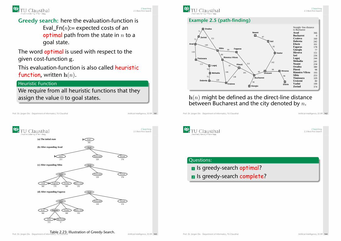
Greedy search: here the evaluation-function isEval_Fn(n):= expected costs of anoptimal path from the state in n to agoal state.
The word optimal is used with respect to thegiven cost-function g.
This evaluation-function is also called heuristicfunction, written h(n).Heuristic Function
We require from all heuristic functions that theyassign the value 0 to goal states.
Prof. Dr. Jürgen Dix · Department of Informatics, TU Clausthal Artificial Intelligence, SS 09 141
2 Searching2.3 Best-First Search
Example 2.5 (path-finding)
Bucharest
Giurgiu
Urziceni
Hirsova
Eforie
NeamtOradea
Zerind
Arad
Timisoara
LugojMehadia
DobretaCraiova
Sibiu
Fagaras
PitestiRimnicu Vilcea
Vaslui
Iasi
Straight−line distanceto Bucharest
0160242161
77151
241
366
193
178
253329
80199
244
380
226
234
374
98
Giurgiu
UrziceniHirsova
Eforie
Neamt
Oradea
Zerind
Arad
Timisoara
Lugoj
Mehadia
Dobreta
Craiova
Sibiu Fagaras
Pitesti
Vaslui
Iasi
Rimnicu Vilcea
Bucharest
71
75
118
111
70
75
120
151
140
99
80
97
101
211
138
146 85
90
98
142
92
87
86
h(n) might be defined as the direct-line distancebetween Bucharest and the city denoted by n.
Prof. Dr. Jürgen Dix · Department of Informatics, TU Clausthal Artificial Intelligence, SS 09 142
2 Searching2.3 Best-First Search
Rimnicu Vilcea
Zerind
Arad
Sibiu
Arad Fagaras Oradea
Timisoara
Sibiu Bucharest
329 374
366 380 193
253 0
Rimnicu Vilcea
Arad
Sibiu
Arad Fagaras Oradea
Timisoara
329
Zerind
374
366 176 380 193
Zerind
Arad
Sibiu Timisoara
253 329 374
Arad
366
(a) The initial state
(b) After expanding Arad
(c) After expanding Sibiu
(d) After expanding Fagaras
Table 2.23: Illustration of Greedy-Search.Prof. Dr. Jürgen Dix · Department of Informatics, TU Clausthal Artificial Intelligence, SS 09 143
2 Searching2.3 Best-First Search
Questions:
1 Is greedy-search optimal?2 Is greedy-search complete?
Prof. Dr. Jürgen Dix · Department of Informatics, TU Clausthal Artificial Intelligence, SS 09 144
2 Searching2.4 A∗ Search
2.4 A∗ Search
Prof. Dr. Jürgen Dix · Department of Informatics, TU Clausthal Artificial Intelligence, SS 09 145
2 Searching2.4 A∗ Search
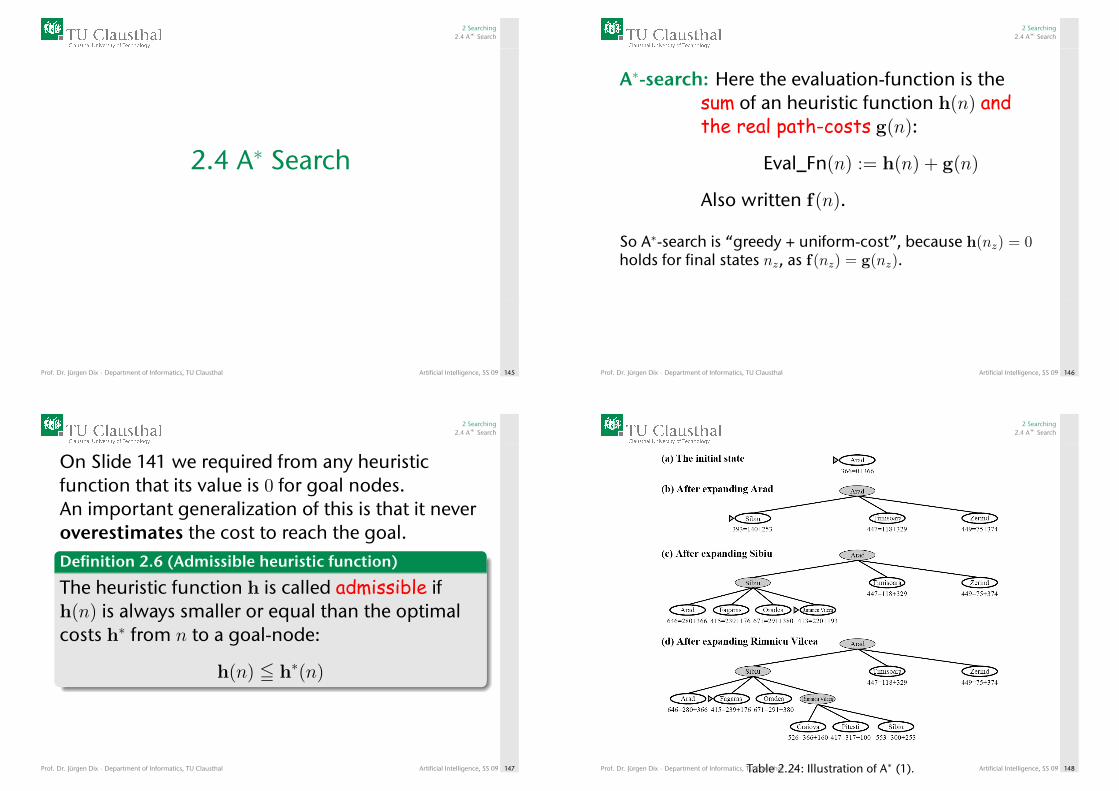
A∗-search: Here the evaluation-function is thesum of an heuristic function h(n) andthe real path-costs g(n):
Eval_Fn(n) := h(n) + g(n)
Also written f(n).
So A∗-search is “greedy + uniform-cost”, because h(nz) = 0holds for final states nz, as f(nz) = g(nz).
Prof. Dr. Jürgen Dix · Department of Informatics, TU Clausthal Artificial Intelligence, SS 09 146
2 Searching2.4 A∗ Search
On Slide 141 we required from any heuristicfunction that its value is 0 for goal nodes.An important generalization of this is that it neveroverestimates the cost to reach the goal.Definition 2.6 (Admissible heuristic function)
The heuristic function h is called admissible ifh(n) is always smaller or equal than the optimalcosts h∗ from n to a goal-node:
h(n) 5 h∗(n)
Prof. Dr. Jürgen Dix · Department of Informatics, TU Clausthal Artificial Intelligence, SS 09 147
2 Searching2.4 A∗ Search
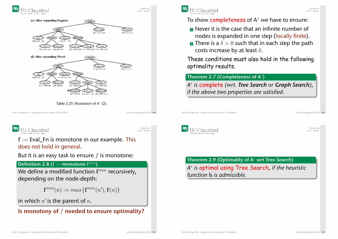
Table 2.24: Illustration of A∗ (1).Prof. Dr. Jürgen Dix · Department of Informatics, TU Clausthal Artificial Intelligence, SS 09 148
2 Searching2.4 A∗ Search
Table 2.25: Illustration of A∗ (2).
Prof. Dr. Jürgen Dix · Department of Informatics, TU Clausthal Artificial Intelligence, SS 09 149
2 Searching2.4 A∗ Search
To show completeness of A∗ we have to ensure:
1 Never it is the case that an infinite number ofnodes is expanded in one step (locally finite).
2 There is a δ > 0 such that in each step the pathcosts increase by at least δ.
These conditions must also hold in the followingoptimality results.
Theorem 2.7 (Completeness of A∗)
A∗ is complete (wrt. Tree Search or Graph Search),if the above two properties are satisfied.
Prof. Dr. Jürgen Dix · Department of Informatics, TU Clausthal Artificial Intelligence, SS 09 150
2 Searching2.4 A∗ Search
f := Eval_Fn is monotone in our example. Thisdoes not hold in general.
But it is an easy task to ensure f is monotone:Definition 2.8 (f monotone fmon)
We define a modified function fmon recursively,depending on the node-depth:
fmon(n) := max{fmon(n′), f(n)}
in which n′ is the parent of n.
Is monotony of f needed to ensure optimality?
Prof. Dr. Jürgen Dix · Department of Informatics, TU Clausthal Artificial Intelligence, SS 09 151
2 Searching2.4 A∗ Search
Theorem 2.9 (Optimality of A∗ wrt Tree Search)
A∗ is optimal using Tree Search, if the heuristicfunction h is admissible.
Prof. Dr. Jürgen Dix · Department of Informatics, TU Clausthal Artificial Intelligence, SS 09 152
2 Searching2.4 A∗ Search
O
Z
A
T
L
M
DC
R
F
P
G
BU
H
E
V
I
N
380
400
420
S
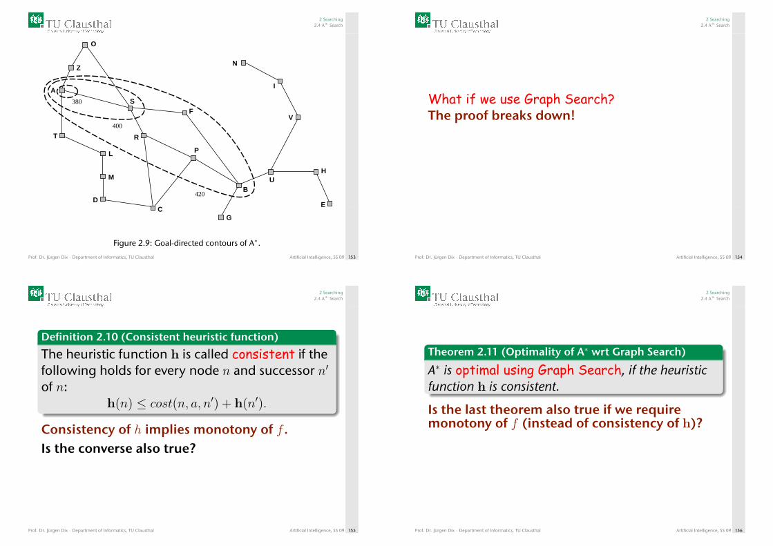
Figure 2.9: Goal-directed contours of A∗.
Prof. Dr. Jürgen Dix · Department of Informatics, TU Clausthal Artificial Intelligence, SS 09 153
2 Searching2.4 A∗ Search
What if we use Graph Search?The proof breaks down!
Prof. Dr. Jürgen Dix · Department of Informatics, TU Clausthal Artificial Intelligence, SS 09 154
2 Searching2.4 A∗ Search
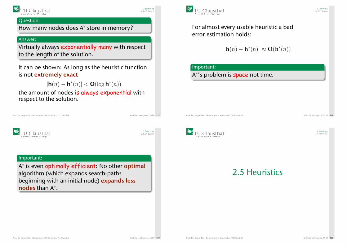
Definition 2.10 (Consistent heuristic function)
The heuristic function h is called consistent if thefollowing holds for every node n and successor n′
of n:h(n) ≤ cost(n, a, n′) + h(n′).
Consistency of h implies monotony of f .Is the converse also true?
Prof. Dr. Jürgen Dix · Department of Informatics, TU Clausthal Artificial Intelligence, SS 09 155
2 Searching2.4 A∗ Search
Theorem 2.11 (Optimality of A∗ wrt Graph Search)
A∗ is optimal using Graph Search, if the heuristicfunction h is consistent.
Is the last theorem also true if we requiremonotony of f (instead of consistency of h)?
Prof. Dr. Jürgen Dix · Department of Informatics, TU Clausthal Artificial Intelligence, SS 09 156
2 Searching2.4 A∗ Search
Question:
How many nodes does A∗ store in memory?
Answer:
Virtually always exponentially many with respectto the length of the solution.
It can be shown: As long as the heuristic functionis not extremely exact
|h(n)− h∗(n)| < O(log h∗(n))
the amount of nodes is always exponential withrespect to the solution.
Prof. Dr. Jürgen Dix · Department of Informatics, TU Clausthal Artificial Intelligence, SS 09 157
2 Searching2.4 A∗ Search
For almost every usable heuristic a baderror-estimation holds:
|h(n)− h∗(n)| ≈ O(h∗(n))
Important:
A∗’s problem is space not time.
Prof. Dr. Jürgen Dix · Department of Informatics, TU Clausthal Artificial Intelligence, SS 09 158
2 Searching2.4 A∗ Search
Important:
A∗ is even optimally efficient: No other optimalalgorithm (which expands search-pathsbeginning with an initial node) expands lessnodes than A∗.
Prof. Dr. Jürgen Dix · Department of Informatics, TU Clausthal Artificial Intelligence, SS 09 159
2 Searching2.5 Heuristics
2.5 Heuristics
Prof. Dr. Jürgen Dix · Department of Informatics, TU Clausthal Artificial Intelligence, SS 09 160
2 Searching2.5 Heuristics
2
Start State Goal State
1
3 4
6 7
5
1
2
3
4
6
7
8
5
8
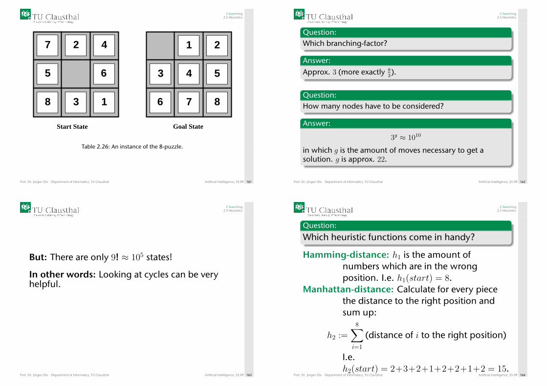
Table 2.26: An instance of the 8-puzzle.
Prof. Dr. Jürgen Dix · Department of Informatics, TU Clausthal Artificial Intelligence, SS 09 161
2 Searching2.5 Heuristics
Question:Which branching-factor?
Answer:Approx. 3 (more exactly 8
3).
Question:How many nodes have to be considered?
Answer:
3g ≈ 1010
in which g is the amount of moves necessary to get asolution. g is approx. 22.
Prof. Dr. Jürgen Dix · Department of Informatics, TU Clausthal Artificial Intelligence, SS 09 162
2 Searching2.5 Heuristics
But: There are only 9! ≈ 105 states!
In other words: Looking at cycles can be veryhelpful.
Prof. Dr. Jürgen Dix · Department of Informatics, TU Clausthal Artificial Intelligence, SS 09 163
2 Searching2.5 Heuristics
Question:
Which heuristic functions come in handy?
Hamming-distance: h1 is the amount ofnumbers which are in the wrongposition. I.e. h1(start) = 8.
Manhattan-distance: Calculate for every piecethe distance to the right position andsum up:
h2 :=8∑i=1
(distance of i to the right position)
I.e.h2(start) = 2+3+2+1+2+2+1+2 = 15.
Prof. Dr. Jürgen Dix · Department of Informatics, TU Clausthal Artificial Intelligence, SS 09 164
2 Searching2.5 Heuristics
Question:
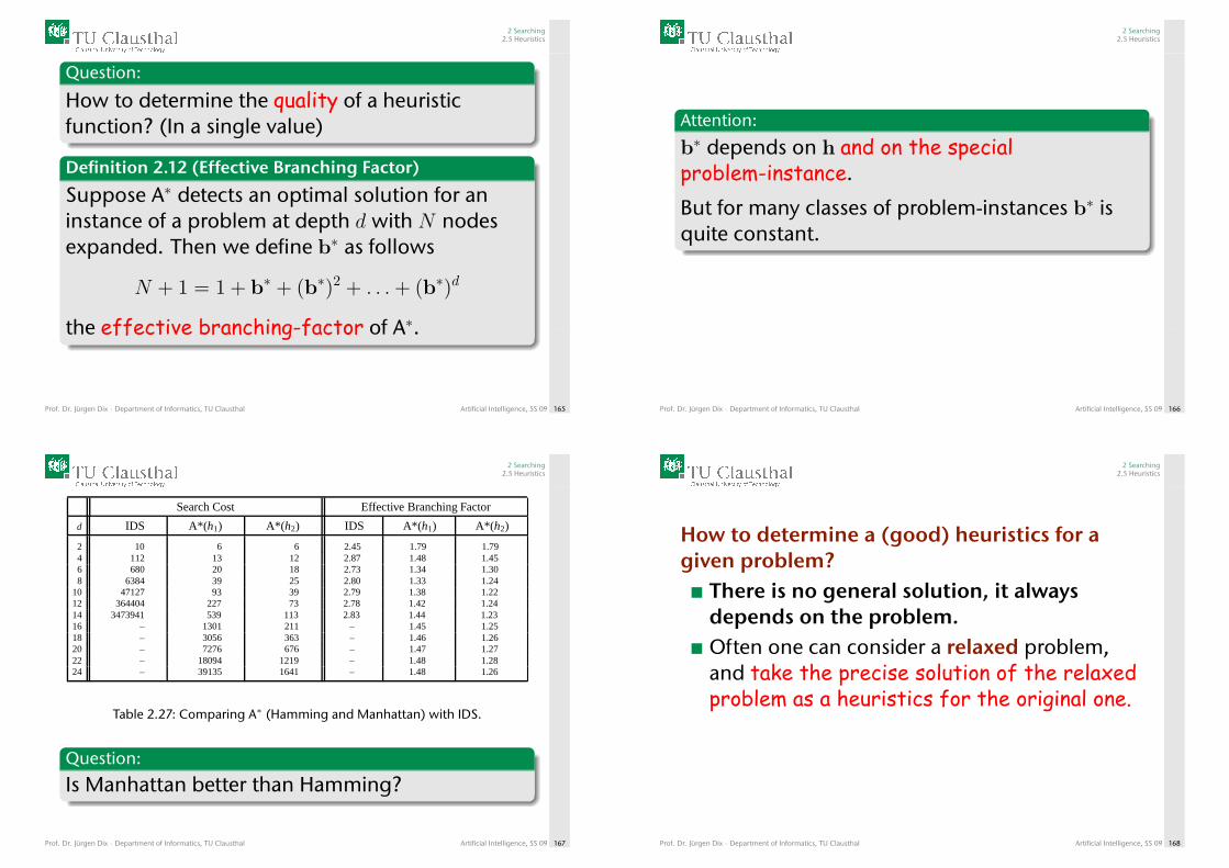
How to determine the quality of a heuristicfunction? (In a single value)
Definition 2.12 (Effective Branching Factor)
Suppose A∗ detects an optimal solution for aninstance of a problem at depth d with N nodesexpanded. Then we define b∗ as follows
N + 1 = 1 + b∗ + (b∗)2 + . . .+ (b∗)d
the effective branching-factor of A∗.
Prof. Dr. Jürgen Dix · Department of Informatics, TU Clausthal Artificial Intelligence, SS 09 165
2 Searching2.5 Heuristics
Attention:
b∗ depends on h and on the specialproblem-instance.
But for many classes of problem-instances b∗ isquite constant.
Prof. Dr. Jürgen Dix · Department of Informatics, TU Clausthal Artificial Intelligence, SS 09 166
2 Searching2.5 Heuristics
Search Cost Effective Branching Factor
d IDS A*(h1) A*(h2) IDS A*(h1) A*(h2)
2 10 6 6 2.45 1.79 1.794 112 13 12 2.87 1.48 1.456 680 20 18 2.73 1.34 1.308 6384 39 25 2.80 1.33 1.24
10 47127 93 39 2.79 1.38 1.2212 364404 227 73 2.78 1.42 1.2414 3473941 539 113 2.83 1.44 1.2316 – 1301 211 – 1.45 1.2518 – 3056 363 – 1.46 1.2620 – 7276 676 – 1.47 1.2722 – 18094 1219 – 1.48 1.2824 – 39135 1641 – 1.48 1.26
Table 2.27: Comparing A∗ (Hamming and Manhattan) with IDS.
Question:
Is Manhattan better than Hamming?
Prof. Dr. Jürgen Dix · Department of Informatics, TU Clausthal Artificial Intelligence, SS 09 167
2 Searching2.5 Heuristics
How to determine a (good) heuristics for agiven problem?
There is no general solution, it alwaysdepends on the problem.Often one can consider a relaxed problem,and take the precise solution of the relaxedproblem as a heuristics for the original one.
Prof. Dr. Jürgen Dix · Department of Informatics, TU Clausthal Artificial Intelligence, SS 09 168
2 Searching2.5 Heuristics
2
Start State Goal State
1
3 6
7 8
5
1
2
3
4
6
8
5 4
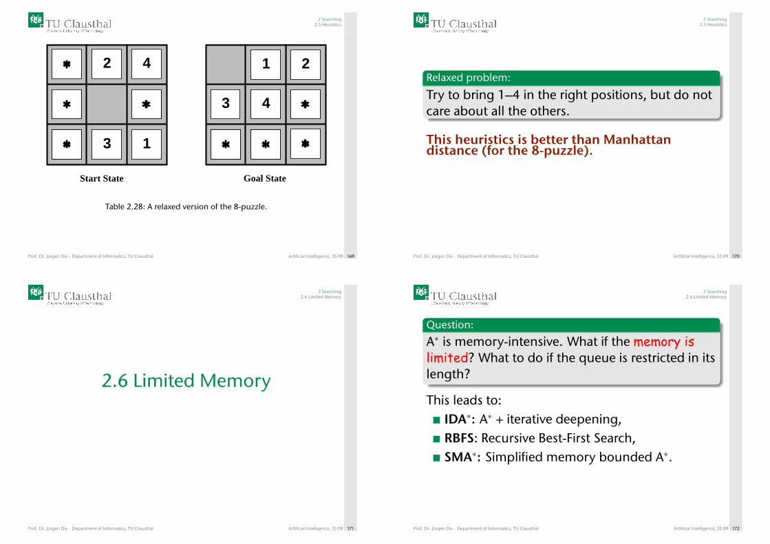
Table 2.28: A relaxed version of the 8-puzzle.
Prof. Dr. Jürgen Dix · Department of Informatics, TU Clausthal Artificial Intelligence, SS 09 169
2 Searching2.5 Heuristics
Relaxed problem:
Try to bring 1–4 in the right positions, but do notcare about all the others.
This heuristics is better than Manhattandistance (for the 8-puzzle).
Prof. Dr. Jürgen Dix · Department of Informatics, TU Clausthal Artificial Intelligence, SS 09 170
2 Searching2.6 Limited Memory
2.6 Limited Memory
Prof. Dr. Jürgen Dix · Department of Informatics, TU Clausthal Artificial Intelligence, SS 09 171
2 Searching2.6 Limited Memory
Question:
A∗ is memory-intensive. What if the memory islimited? What to do if the queue is restricted in itslength?
This leads to:IDA∗: A∗ + iterative deepening,RBFS: Recursive Best-First Search,SMA∗: Simplified memory bounded A∗.
Prof. Dr. Jürgen Dix · Department of Informatics, TU Clausthal Artificial Intelligence, SS 09 172
2 Searching2.6 Limited Memory
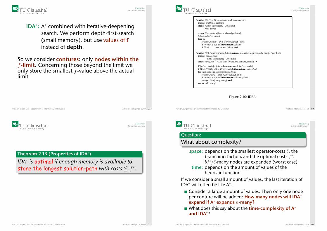
IDA∗: A∗ combined with iterative-deepeningsearch. We perform depth-first-search(small memory), but use values of finstead of depth.
So we consider contures: only nodes within thef -limit. Concerning those beyond the limit weonly store the smallest f -value above the actuallimit.
Prof. Dr. Jürgen Dix · Department of Informatics, TU Clausthal Artificial Intelligence, SS 09 173
2 Searching2.6 Limited Memory
function IDA*( problem) returns a solution sequenceinputs: problem, a problemstatic: f-limit, the current f - COST limit
root, a node
root�MAKE-NODE(INITIAL-STATE[problem])f-limit� f - COST(root)loop do
solution, f-limit�DFS-CONTOUR(root, f-limit)if solution is non-null then return solutionif f-limit =� then return failure; end
function DFS-CONTOUR(node, f-limit) returns a solution sequence and a new f - COST limitinputs: node, a node
f-limit, the current f - COST limitstatic: next-f, the f - COST limit for the next contour, initially�
if f - COST[node] > f-limit then return null, f - COST[node]if GOAL-TEST[problem](STATE[node]) then return node, f-limitfor each node s in SUCCESSORS(node) do
solution, new-f�DFS-CONTOUR(s, f-limit)if solution is non-null then return solution, f-limitnext-f�MIN(next-f, new-f); end
return null, next-f
Figure 2.10: IDA∗.
Prof. Dr. Jürgen Dix · Department of Informatics, TU Clausthal Artificial Intelligence, SS 09 174
2 Searching2.6 Limited Memory
Theorem 2.13 (Properties of IDA∗)
IDA∗ is optimal if enough memory is available tostore the longest solution-path with costs 5 f ∗.
Prof. Dr. Jürgen Dix · Department of Informatics, TU Clausthal Artificial Intelligence, SS 09 175
2 Searching2.6 Limited Memory
Question:
What about complexity?
space: depends on the smallest operator-costs δ, thebranching-factor b and the optimal costs f ∗.bf ∗/δ-many nodes are expanded (worst case)
time: depends on the amount of values of theheuristic function.
If we consider a small amount of values, the last iteration ofIDA∗ will often be like A∗.
Consider a large amount of values. Then only one nodeper conture will be added: How many nodes will IDA∗
expand if A∗ expands n-many?What does this say about the time-complexity of A∗
and IDA∗?
Prof. Dr. Jürgen Dix · Department of Informatics, TU Clausthal Artificial Intelligence, SS 09 176
2 Searching2.6 Limited Memory
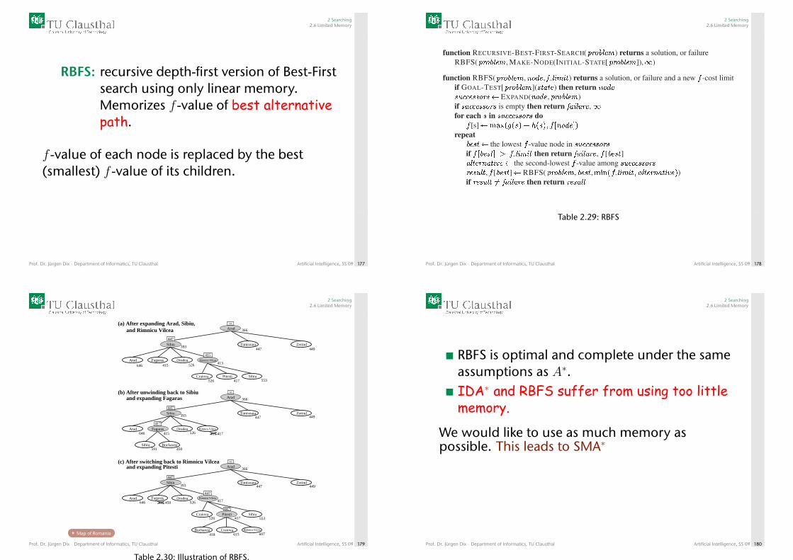
RBFS: recursive depth-first version of Best-Firstsearch using only linear memory.Memorizes f -value of best alternativepath.
f -value of each node is replaced by the best(smallest) f -value of its children.
Prof. Dr. Jürgen Dix · Department of Informatics, TU Clausthal Artificial Intelligence, SS 09 177
2 Searching2.6 Limited Memory
function RECURSIVE-BEST-FIRST-SEARCH( � � � � � � ) returns a solution, or failureRBFS( � � � � � � , MAKE-NODE(INITIAL-STATE[ � � � � � � ]), � )
function RBFS( � � � � � � , � � � , � � � � � � ) returns a solution, or failure and a new � -cost limitif GOAL-TEST[ � � � � � � ]( � � � � ) then return � � �
� " " � � � � � $ EXPAND( � � � , � � � � � � )if � " " � � � � � is empty then return � � � � � , �for each � in � " " � � � � � do
� [s] $ * , - / 0 / � 2 4 6 / � 2 7 � 9 � � � : 2repeat
� � � $ the lowest � -value node in � " " � � � � �if � 9 � � � : = � � � � � � then return � � � � � , � [ � � � ]
� � � � � � � � B $ the second-lowest � -value among � " " � � � � �� � � � , � [ � � � ] $ RBFS( � � � � � � , � � � , * F H / � � � � � � 7 � � � � � � � � B 2 )if � � � � KL � � � � � then return � � � �
Table 2.29: RBFS
Prof. Dr. Jürgen Dix · Department of Informatics, TU Clausthal Artificial Intelligence, SS 09 178
2 Searching2.6 Limited Memory
Map of Romania
Zerind
Arad
Sibiu
Arad Fagaras Oradea
Craiova Sibiu
Bucharest Craiova Rimnicu Vilcea
Zerind
Arad
Sibiu
Arad
Sibiu Bucharest
Rimnicu VilceaOradea
Zerind
Arad
Sibiu
Arad
Timisoara
Timisoara
Timisoara
Fagaras Oradea Rimnicu Vilcea
Craiova Pitesti Sibiu
646 415 526
526 553
646 526
450591
646 526
526 553
418 615 607
447 449
447
447 449
449
366
393
366
393
413
413 417415
366
393
415 450 417Rimnicu Vilcea
Fagaras
447
415
447
447
417
(a) After expanding Arad, Sibiu, and Rimnicu Vilcea
(c) After switching back to Rimnicu Vilcea and expanding Pitesti
(b) After unwinding back to Sibiu and expanding Fagaras
447
447
∞
∞
∞
417
417
Pitesti
Table 2.30: Illustration of RBFS.
Prof. Dr. Jürgen Dix · Department of Informatics, TU Clausthal Artificial Intelligence, SS 09 179
2 Searching2.6 Limited Memory
RBFS is optimal and complete under the sameassumptions as A∗.IDA∗ and RBFS suffer from using too littlememory.
We would like to use as much memory aspossible. This leads to SMA∗
Prof. Dr. Jürgen Dix · Department of Informatics, TU Clausthal Artificial Intelligence, SS 09 180
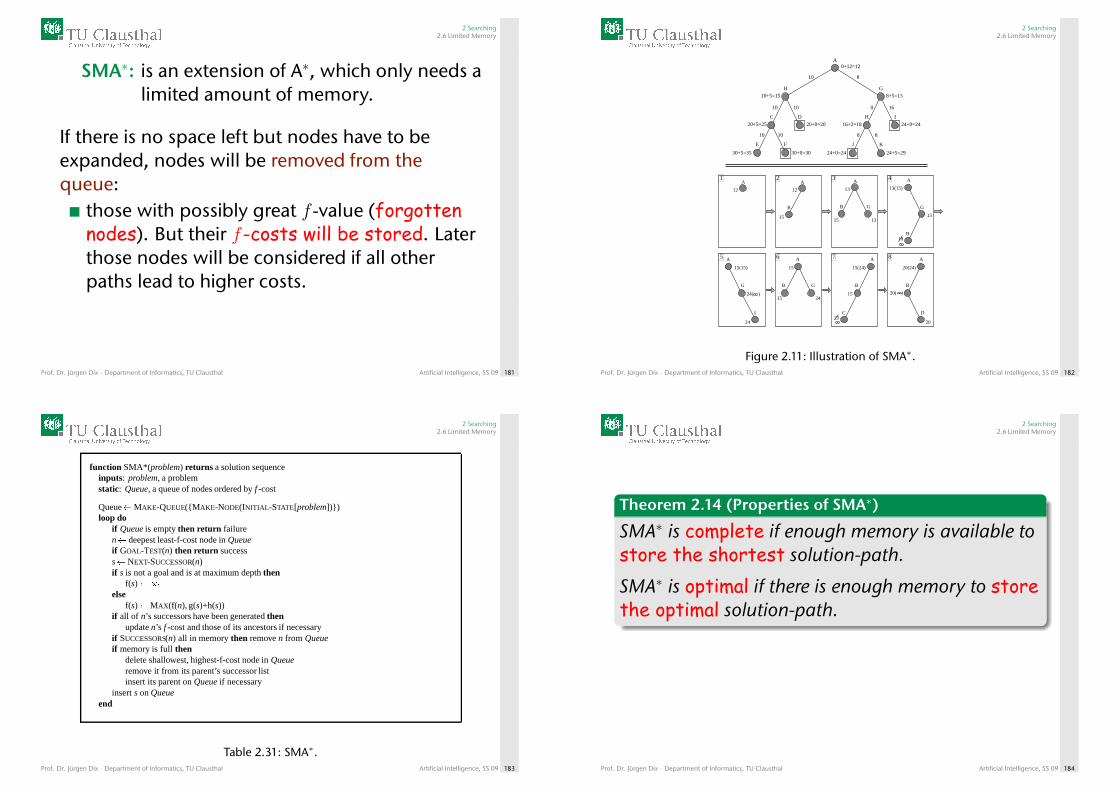
2 Searching2.6 Limited Memory
SMA∗: is an extension of A∗, which only needs alimited amount of memory.
If there is no space left but nodes have to beexpanded, nodes will be removed from thequeue:
those with possibly great f -value (forgottennodes). But their f-costs will be stored. Laterthose nodes will be considered if all otherpaths lead to higher costs.
Prof. Dr. Jürgen Dix · Department of Informatics, TU Clausthal Artificial Intelligence, SS 09 181
2 Searching2.6 Limited Memory
0+12=12
10 8
10 10 8
8 810 10
10+5=15 8+5=13
20+5=25 20+0=20 16+2=18
24+0=24 24+5=2930+5=35 30+0=30
16
24+0=24
A
B
C D
E F
G
H I
J K
15 24
A
B G
15
15 13
13
A
B G
12
15
A
B
12
A
24
A
G
I
15(15)
24( )
20
A
B
D
20(24)
20( )15
25
A
B
C
15(24)
13
18
A
G
H
13(15)
41 2 3
5 6 7 8
Figure 2.11: Illustration of SMA∗.Prof. Dr. Jürgen Dix · Department of Informatics, TU Clausthal Artificial Intelligence, SS 09 182
2 Searching2.6 Limited Memory
function SMA*(problem) returns a solution sequenceinputs: problem, a problemstatic: Queue, a queue of nodes ordered by f -cost
Queue�MAKE-QUEUE({MAKE-NODE(INITIAL-STATE[problem])})loop do
if Queue is empty then return failuren� deepest least-f-cost node in Queueif GOAL-TEST(n) then return successs�NEXT-SUCCESSOR(n)if s is not a goal and is at maximum depth then
f(s)��else
f(s)�MAX(f(n), g(s)+h(s))if all of n’s successors have been generated then
update n’s f -cost and those of its ancestors if necessaryif SUCCESSORS(n) all in memory then remove n from Queueif memory is full then
delete shallowest, highest-f-cost node in Queueremove it from its parent’s successor listinsert its parent on Queue if necessary
insert s on Queueend
Table 2.31: SMA∗.Prof. Dr. Jürgen Dix · Department of Informatics, TU Clausthal Artificial Intelligence, SS 09 183
2 Searching2.6 Limited Memory
Theorem 2.14 (Properties of SMA∗)
SMA∗ is complete if enough memory is available tostore the shortest solution-path.
SMA∗ is optimal if there is enough memory to storethe optimal solution-path.
Prof. Dr. Jürgen Dix · Department of Informatics, TU Clausthal Artificial Intelligence, SS 09 184
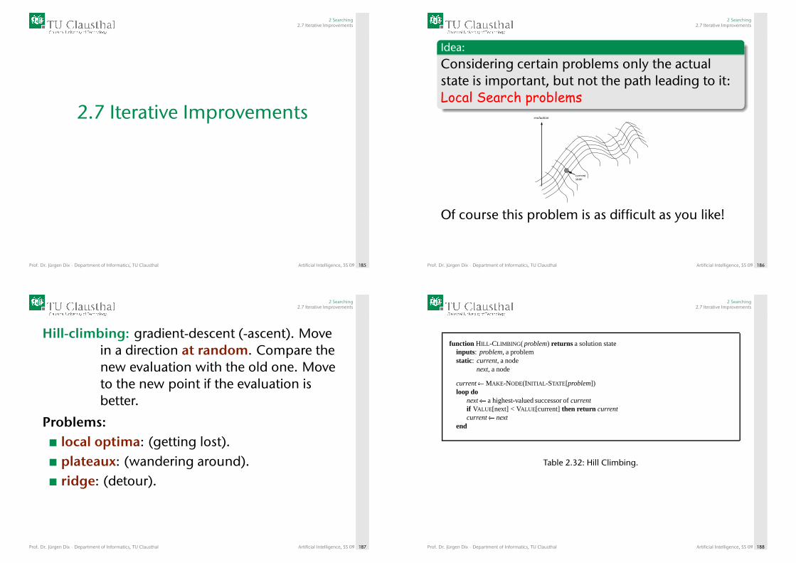
2 Searching2.7 Iterative Improvements
2.7 Iterative Improvements
Prof. Dr. Jürgen Dix · Department of Informatics, TU Clausthal Artificial Intelligence, SS 09 185
2 Searching2.7 Iterative Improvements
Idea:
Considering certain problems only the actualstate is important, but not the path leading to it:Local Search problems
evaluation
currentstate
Of course this problem is as difficult as you like!
Prof. Dr. Jürgen Dix · Department of Informatics, TU Clausthal Artificial Intelligence, SS 09 186
2 Searching2.7 Iterative Improvements
Hill-climbing: gradient-descent (-ascent). Movein a direction at random. Compare thenew evaluation with the old one. Moveto the new point if the evaluation isbetter.
Problems:local optima: (getting lost).plateaux: (wandering around).ridge: (detour).
Prof. Dr. Jürgen Dix · Department of Informatics, TU Clausthal Artificial Intelligence, SS 09 187
2 Searching2.7 Iterative Improvements
function HILL-CLIMBING( problem) returns a solution stateinputs: problem, a problemstatic: current, a node
next, a node
current�MAKE-NODE(INITIAL-STATE[problem])loop do
next� a highest-valued successor of currentif VALUE[next] < VALUE[current] then return currentcurrent� next
end
Table 2.32: Hill Climbing.
Prof. Dr. Jürgen Dix · Department of Informatics, TU Clausthal Artificial Intelligence, SS 09 188
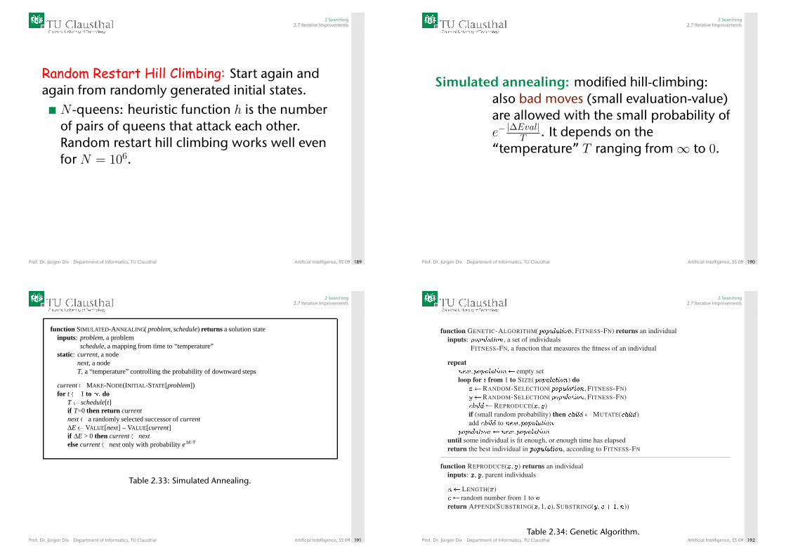
2 Searching2.7 Iterative Improvements
Random Restart Hill Climbing: Start again andagain from randomly generated initial states.
N -queens: heuristic function h is the numberof pairs of queens that attack each other.Random restart hill climbing works well evenfor N = 106.
Prof. Dr. Jürgen Dix · Department of Informatics, TU Clausthal Artificial Intelligence, SS 09 189
2 Searching2.7 Iterative Improvements
Simulated annealing: modified hill-climbing:also bad moves (small evaluation-value)are allowed with the small probability ofe− |∆Eval|T . It depends on the“temperature” T ranging from∞ to 0.
Prof. Dr. Jürgen Dix · Department of Informatics, TU Clausthal Artificial Intelligence, SS 09 190
2 Searching2.7 Iterative Improvements
function SIMULATED-ANNEALING( problem, schedule) returns a solution stateinputs: problem, a problem
schedule, a mapping from time to “temperature”static: current, a node
next, a nodeT, a “temperature” controlling the probability of downward steps
current�MAKE-NODE(INITIAL-STATE[problem])for t� 1 to� do
T� schedule[t]if T=0 then return currentnext� a randomly selected successor of currentΔE�VALUE[next] – VALUE[current]if ΔE > 0 then current� nextelse current� next only with probability eΔE/T
Table 2.33: Simulated Annealing.
Prof. Dr. Jürgen Dix · Department of Informatics, TU Clausthal Artificial Intelligence, SS 09 191
2 Searching2.7 Iterative Improvements
function GENETIC-ALGORITHM( � � � � � � � � , FITNESS-FN) returns an individualinputs: � � � � � � � � , a set of individuals
FITNESS-FN, a function that measures the fitness of an individual
repeat� � � � � � � � � � � � empty setloop for from 1 to SIZE( � � � � � � � � ) do
� � RANDOM-SELECTION( � � � � � � � � , FITNESS-FN)� � RANDOM-SELECTION( � � � � � � � � , FITNESS-FN)� � � " � REPRODUCE( � , � )if (small random probability) then � � � " � MUTATE( � � � " )add � � � " to � � � � � � � � � � �
� � � � � � � � � � � � � � � � � � � �
until some individual is fit enough, or enough time has elapsedreturn the best individual in � � � � � � � � , according to FITNESS-FN
function REPRODUCE( � , � ) returns an individualinputs: � , � , parent individuals
� � LENGTH( � )� � random number from 1 to �
return APPEND(SUBSTRING( � , 1, � ), SUBSTRING( � , � + - , � ))
Table 2.34: Genetic Algorithm.Prof. Dr. Jürgen Dix · Department of Informatics, TU Clausthal Artificial Intelligence, SS 09 192
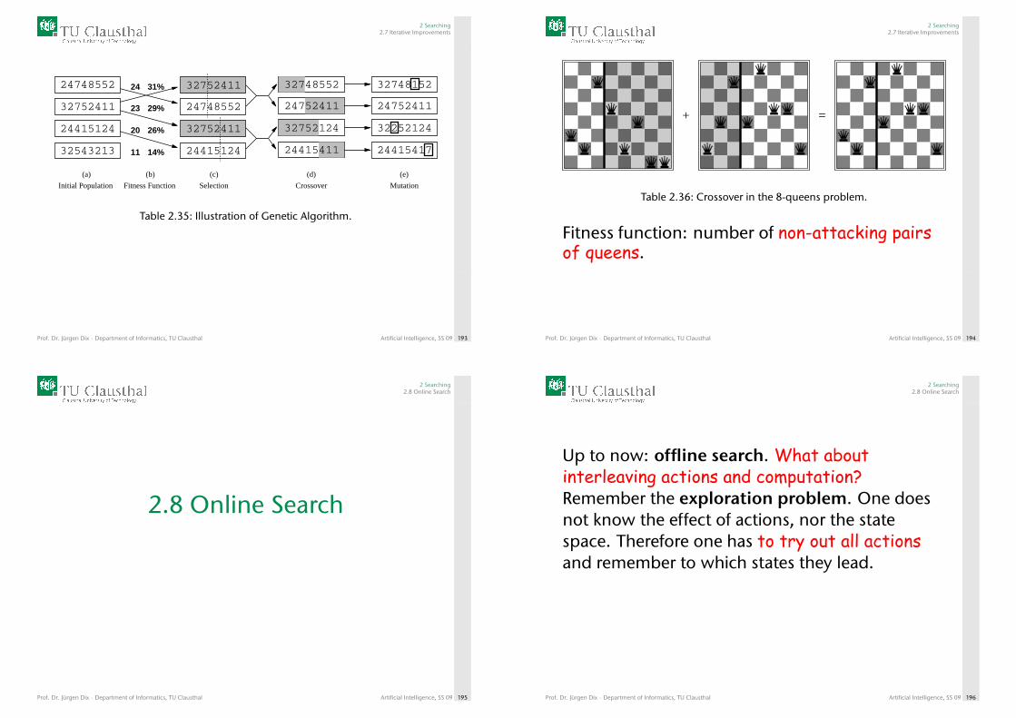
2 Searching2.7 Iterative Improvements
(a)
Initial Population
(b)
Fitness Function
(c)
Selection
(d)
Crossover
(e)
Mutation
24
23
20
11
29%
31%
26%
14%
32752411
24748552
32752411
24415124
32748552
24752411
32752124
24415411
32252124
24752411
32748152
24415417
24748552
32752411
24415124
32543213
Table 2.35: Illustration of Genetic Algorithm.
Prof. Dr. Jürgen Dix · Department of Informatics, TU Clausthal Artificial Intelligence, SS 09 193
2 Searching2.7 Iterative Improvements
+ =
Table 2.36: Crossover in the 8-queens problem.
Fitness function: number of non-attacking pairsof queens.
Prof. Dr. Jürgen Dix · Department of Informatics, TU Clausthal Artificial Intelligence, SS 09 194
2 Searching2.8 Online Search
2.8 Online Search
Prof. Dr. Jürgen Dix · Department of Informatics, TU Clausthal Artificial Intelligence, SS 09 195
2 Searching2.8 Online Search
Up to now: offline search. What aboutinterleaving actions and computation?Remember the exploration problem. One doesnot know the effect of actions, nor the statespace. Therefore one has to try out all actionsand remember to which states they lead.
Prof. Dr. Jürgen Dix · Department of Informatics, TU Clausthal Artificial Intelligence, SS 09 196
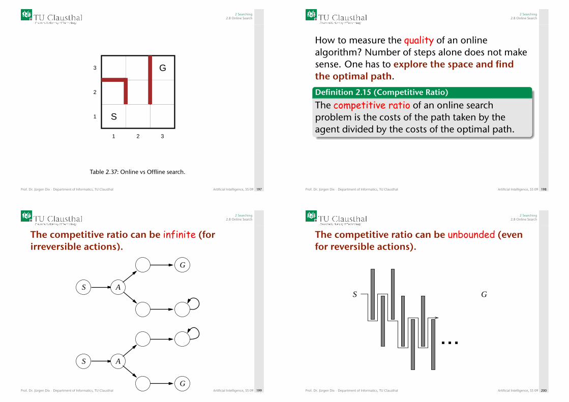
2 Searching2.8 Online Search
G
S
1 2 3
1
2
3
Table 2.37: Online vs Offline search.
Prof. Dr. Jürgen Dix · Department of Informatics, TU Clausthal Artificial Intelligence, SS 09 197
2 Searching2.8 Online Search
How to measure the quality of an onlinealgorithm? Number of steps alone does not makesense. One has to explore the space and findthe optimal path.
Definition 2.15 (Competitive Ratio)
The competitive ratio of an online searchproblem is the costs of the path taken by theagent divided by the costs of the optimal path.
Prof. Dr. Jürgen Dix · Department of Informatics, TU Clausthal Artificial Intelligence, SS 09 198
2 Searching2.8 Online Search
The competitive ratio can be infinite (forirreversible actions).
S
G
S
G
A
A
Table 2.38: Competitive Ratio.
Prof. Dr. Jürgen Dix · Department of Informatics, TU Clausthal Artificial Intelligence, SS 09 199
2 Searching2.8 Online Search
The competitive ratio can be unbounded (evenfor reversible actions).
S G
Table 2.39: Unbounded Competitive Ratio.
Prof. Dr. Jürgen Dix · Department of Informatics, TU Clausthal Artificial Intelligence, SS 09 200
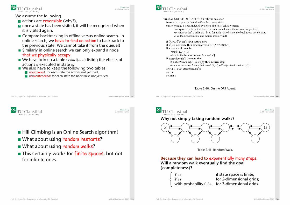
2 Searching2.8 Online Search
We assume the following1 actions are reversible (why?),2 once a state has been visited, it will be recognized when
it is visited again.Compare backtracking in offline versus online search. Inonline search, we have to find an action to backtrack tothe previous state. We cannot take it from the queue!!Similarly in online search we can only expand a nodethat we physically occupy.We have to keep a table result(a, s) listing the effects ofactions a executed in state s.We also have to keep the following two tables:
1 unexplored: for each state the actions not yet tried,2 unbacktracked: for each state the backtracks not yet tried.
Prof. Dr. Jürgen Dix · Department of Informatics, TU Clausthal Artificial Intelligence, SS 09 201
2 Searching2.8 Online Search
Table 2.40: Online DFS Agent.
Prof. Dr. Jürgen Dix · Department of Informatics, TU Clausthal Artificial Intelligence, SS 09 202
2 Searching2.8 Online Search
Hill Climbing is an Online Search algorithm!What about using random restarts?What about using random walks?This certainly works for finite spaces, but notfor infinite ones.
Prof. Dr. Jürgen Dix · Department of Informatics, TU Clausthal Artificial Intelligence, SS 09 203
2 Searching2.8 Online Search
Why not simply taking random walks?
S G
Table 2.41: Random Walk.
Because they can lead to exponentially many steps.Will a random walk eventually find the goal(completeness)? Y es, if state space is finite;
Y es, for 2-dimensional grids;with probability 0.34, for 3-dimensional grids.
Prof. Dr. Jürgen Dix · Department of Informatics, TU Clausthal Artificial Intelligence, SS 09 204
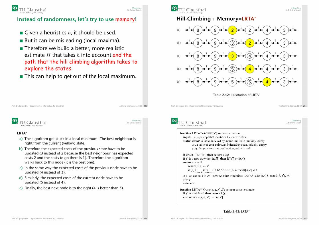
2 Searching2.8 Online Search
Instead of randomness, let’s try to use memory!
Given a heuristics h, it should be used.But it can be misleading (local maxima).Therefore we build a better, more realisticestimate H that takes h into account and thepath that the hill climbing algorithm takes toexplore the states.This can help to get out of the local maximum.
Prof. Dr. Jürgen Dix · Department of Informatics, TU Clausthal Artificial Intelligence, SS 09 205
2 Searching2.8 Online Search
Hill-Climbing + Memory=LRTA∗
12
1 11 1 11
1 1 11 1 11
1 1 11 1 11
8 9
8 9
8 9
2
2
3
4
4
4
3
3
3
1 1 11 1 118 9 4 4 3
1 1 11 1 118 9 4 35
3
5
5
4
(a)
(b)
(c)
(d)
(e)
Table 2.42: Illustration of LRTA∗
Prof. Dr. Jürgen Dix · Department of Informatics, TU Clausthal Artificial Intelligence, SS 09 206
2 Searching2.8 Online Search
LRTA∗
a) The algorithm got stuck in a local minimum. The best neighbour isright from the current (yellow) state.
b) Therefore the expected costs of the previous state have to beupdated (3 instead of 2 because the best neighbour has expectedcosts 2 and the costs to go there is 1). Therefore the algorithmwalks back to this node (it is the best one).
c) In the same way the expected costs of the previous node have to beupdated (4 instead of 3).
d) Similarly, the expected costs of the current node have to beupdated (5 instead of 4).
e) Finally, the best next node is to the right (4 is better than 5).
Prof. Dr. Jürgen Dix · Department of Informatics, TU Clausthal Artificial Intelligence, SS 09 207
2 Searching2.8 Online Search
Table 2.43: LRTA∗
Prof. Dr. Jürgen Dix · Department of Informatics, TU Clausthal Artificial Intelligence, SS 09 208
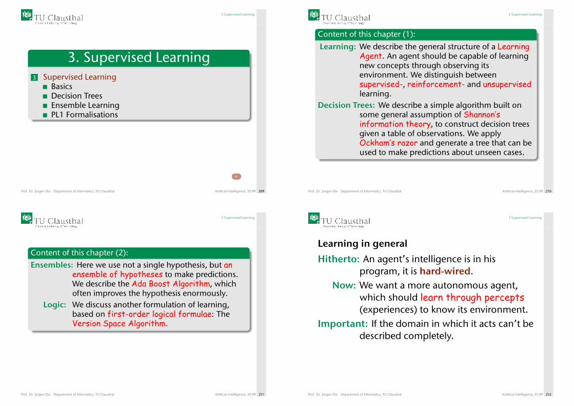
3 Supervised Learning
3. Supervised Learning3 Supervised Learning
BasicsDecision TreesEnsemble LearningPL1 Formalisations
Prof. Dr. Jürgen Dix · Department of Informatics, TU Clausthal Artificial Intelligence, SS 09 209
3 Supervised Learning
Content of this chapter (1):
Learning: We describe the general structure of a LearningAgent. An agent should be capable of learningnew concepts through observing itsenvironment. We distinguish betweensupervised-, reinforcement- and unsupervisedlearning.
Decision Trees: We describe a simple algorithm built onsome general assumption of Shannon’sinformation theory, to construct decision treesgiven a table of observations. We applyOckham’s razor and generate a tree that can beused to make predictions about unseen cases.
Prof. Dr. Jürgen Dix · Department of Informatics, TU Clausthal Artificial Intelligence, SS 09 210
3 Supervised Learning
Content of this chapter (2):
Ensembles: Here we use not a single hypothesis, but anensemble of hypotheses to make predictions.We describe the Ada Boost Algorithm, whichoften improves the hypothesis enormously.
Logic: We discuss another formulation of learning,based on first-order logical formulae: TheVersion Space Algorithm.
Prof. Dr. Jürgen Dix · Department of Informatics, TU Clausthal Artificial Intelligence, SS 09 211
3 Supervised Learning
Learning in general
Hitherto: An agent’s intelligence is in hisprogram, it is hard-wired.
Now: We want a more autonomous agent,which should learn through percepts(experiences) to know its environment.
Important: If the domain in which it acts can’t bedescribed completely.
Prof. Dr. Jürgen Dix · Department of Informatics, TU Clausthal Artificial Intelligence, SS 09 212
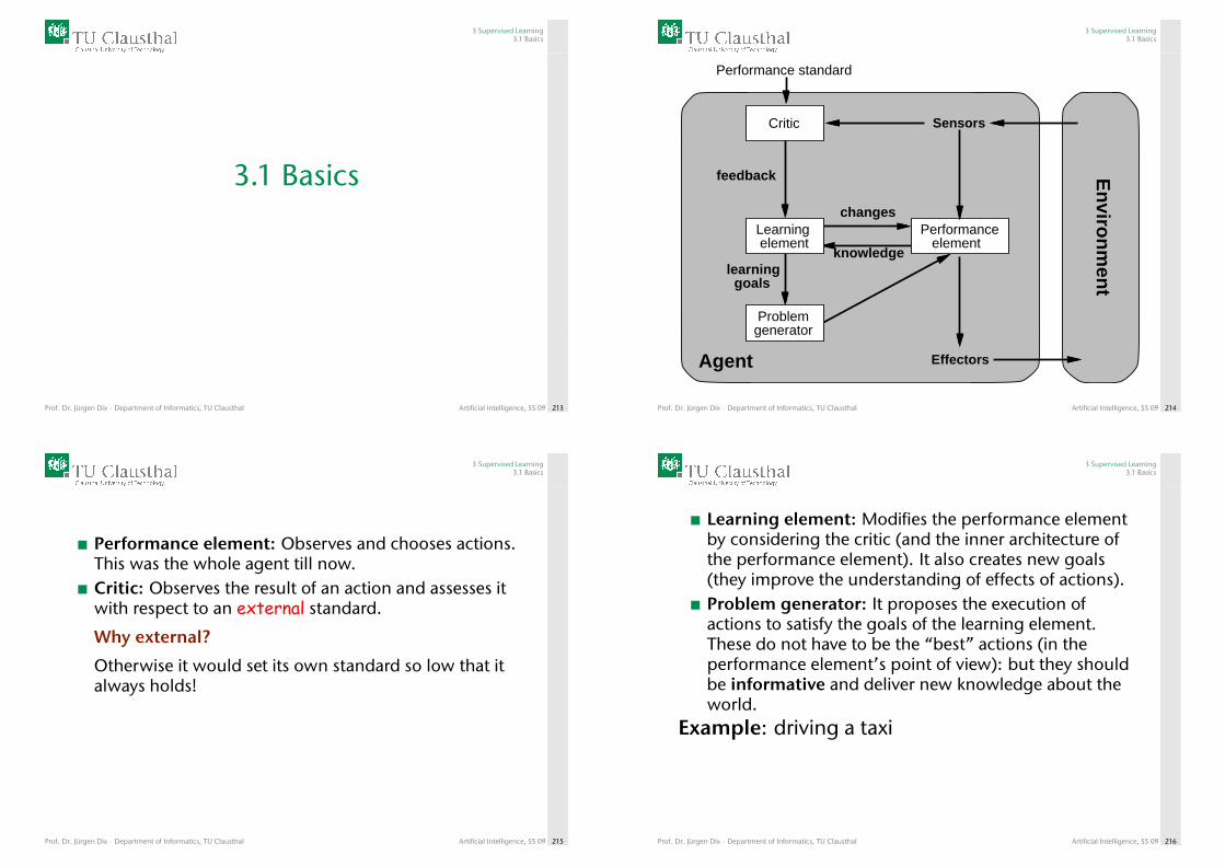
3 Supervised Learning3.1 Basics
3.1 Basics
Prof. Dr. Jürgen Dix · Department of Informatics, TU Clausthal Artificial Intelligence, SS 09 213
3 Supervised Learning3.1 Basics
Performance standard
Agent
En
viron
men
tSensors
Effectors
Performance element
changes
knowledgelearning goals
Problem generator
feedback
Learning element
Critic
Prof. Dr. Jürgen Dix · Department of Informatics, TU Clausthal Artificial Intelligence, SS 09 214
3 Supervised Learning3.1 Basics
Performance element: Observes and chooses actions.This was the whole agent till now.Critic: Observes the result of an action and assesses itwith respect to an external standard.
Why external?
Otherwise it would set its own standard so low that italways holds!
Prof. Dr. Jürgen Dix · Department of Informatics, TU Clausthal Artificial Intelligence, SS 09 215
3 Supervised Learning3.1 Basics
Learning element: Modifies the performance elementby considering the critic (and the inner architecture ofthe performance element). It also creates new goals(they improve the understanding of effects of actions).Problem generator: It proposes the execution ofactions to satisfy the goals of the learning element.These do not have to be the “best” actions (in theperformance element’s point of view): but they shouldbe informative and deliver new knowledge about theworld.
Example: driving a taxi
Prof. Dr. Jürgen Dix · Department of Informatics, TU Clausthal Artificial Intelligence, SS 09 216
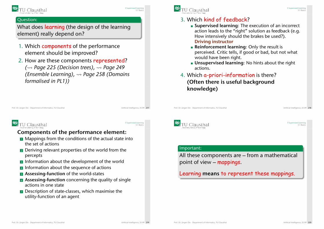
3 Supervised Learning3.1 Basics
Question:
What does learning (the design of the learningelement) really depend on?
1. Which components of the performanceelement should be improved?
2. How are these components represented?( Page 225 (Decision trees), Page 249(Ensemble Learning), Page 258 (Domainsformalised in PL1))
Prof. Dr. Jürgen Dix · Department of Informatics, TU Clausthal Artificial Intelligence, SS 09 217
3 Supervised Learning3.1 Basics
3. Which kind of feedback?Supervised learning: The execution of an incorrectaction leads to the “right” solution as feedback (e.g.How intensively should the brakes be used?).Driving instructorReinforcement learning: Only the result isperceived. Critic tells, if good or bad, but not whatwould have been right.Unsupervised learning: No hints about the rightactions.
4. Which a-priori-information is there?(Often there is useful backgroundknowledge)
Prof. Dr. Jürgen Dix · Department of Informatics, TU Clausthal Artificial Intelligence, SS 09 218
3 Supervised Learning3.1 Basics
Components of the performance element:1 Mappings from the conditions of the actual state into
the set of actions2 Deriving relevant properties of the world from the
percepts3 Information about the development of the world4 Information about the sequence of actions5 Assessing-function of the world-states6 Assessing-function concerning the quality of single
actions in one state7 Description of state-classes, which maximise the
utility-function of an agent
Prof. Dr. Jürgen Dix · Department of Informatics, TU Clausthal Artificial Intelligence, SS 09 219
3 Supervised Learning3.1 Basics
Important:
All these components are – from a mathematicalpoint of view – mappings.
Learning means to represent these mappings.
Prof. Dr. Jürgen Dix · Department of Informatics, TU Clausthal Artificial Intelligence, SS 09 220
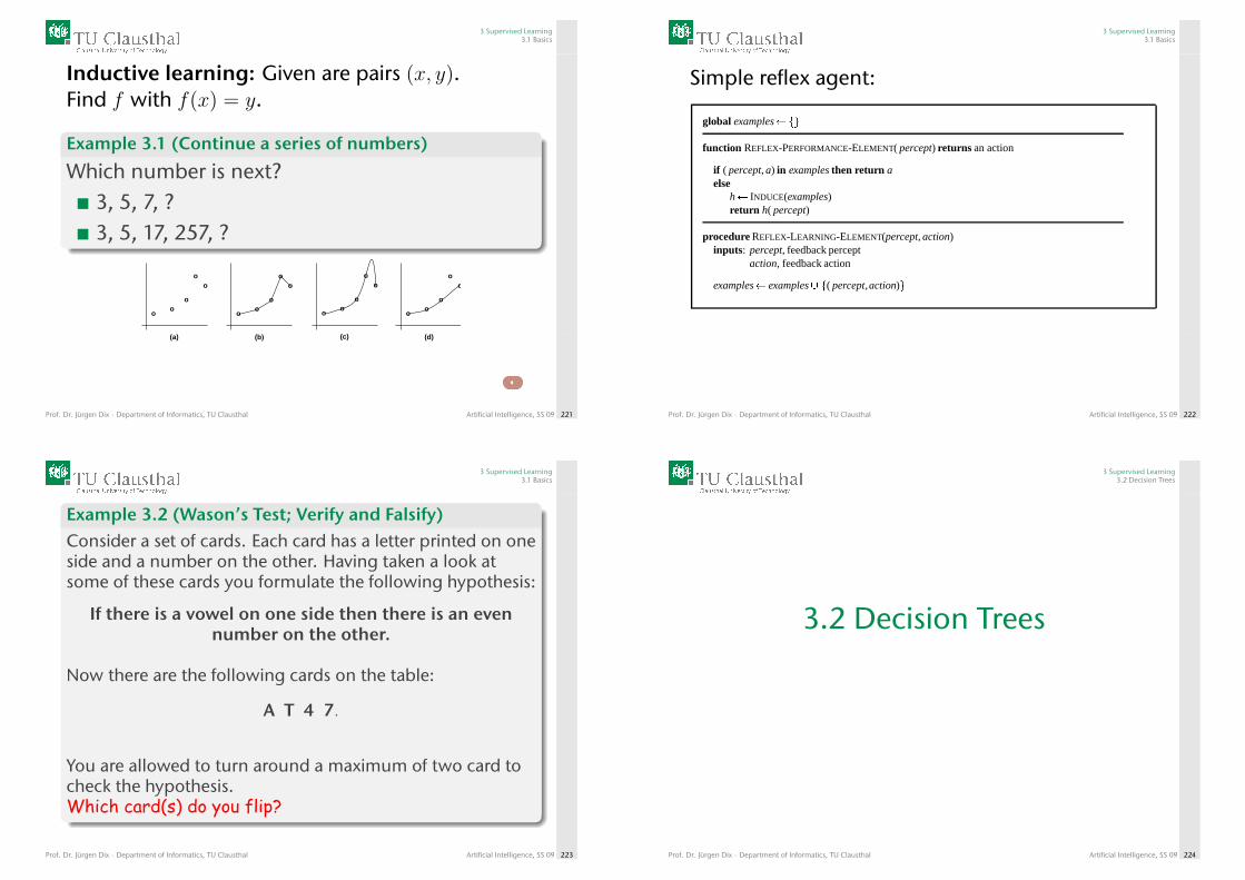
3 Supervised Learning3.1 Basics
Inductive learning: Given are pairs (x, y).Find f with f(x) = y.
Example 3.1 (Continue a series of numbers)
Which number is next?3, 5, 7, ?3, 5, 17, 257, ?
oo
oo
(c)
oo
o
oo
(a)
oo
o
oo
(b)
oo
o
oo
(d)
o
Prof. Dr. Jürgen Dix · Department of Informatics, TU Clausthal Artificial Intelligence, SS 09 221
3 Supervised Learning3.1 Basics
Simple reflex agent:
global examples�fg
function REFLEX-PERFORMANCE-ELEMENT( percept) returns an action
if ( percept, a) in examples then return aelse
h� INDUCE(examples)return h( percept)
procedure REFLEX-LEARNING-ELEMENT(percept, action)inputs: percept, feedback percept
action, feedback action
examples� examples� f( percept,action)g
Prof. Dr. Jürgen Dix · Department of Informatics, TU Clausthal Artificial Intelligence, SS 09 222
3 Supervised Learning3.1 Basics
Example 3.2 (Wason’s Test; Verify and Falsify)Consider a set of cards. Each card has a letter printed on oneside and a number on the other. Having taken a look atsome of these cards you formulate the following hypothesis:
If there is a vowel on one side then there is an evennumber on the other.
Now there are the following cards on the table:
A T 4 7.
You are allowed to turn around a maximum of two card tocheck the hypothesis.Which card(s) do you flip?
Prof. Dr. Jürgen Dix · Department of Informatics, TU Clausthal Artificial Intelligence, SS 09 223
3 Supervised Learning3.2 Decision Trees
3.2 Decision Trees
Prof. Dr. Jürgen Dix · Department of Informatics, TU Clausthal Artificial Intelligence, SS 09 224
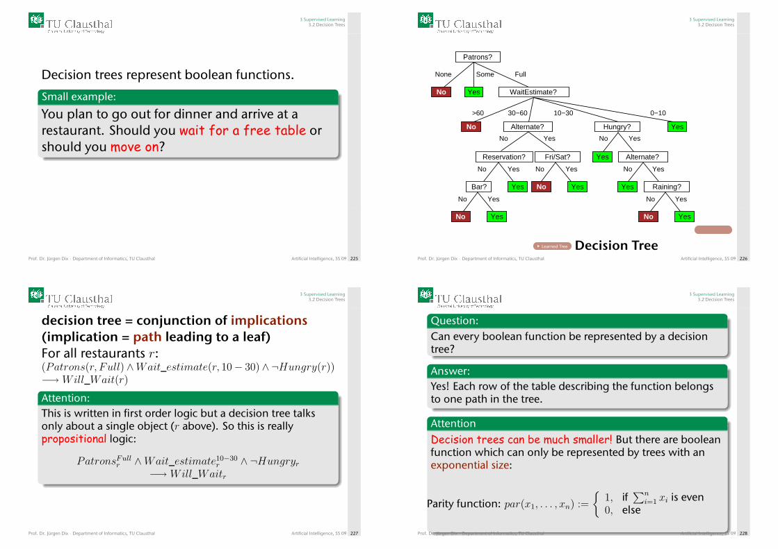
3 Supervised Learning3.2 Decision Trees
Decision trees represent boolean functions.
Small example:
You plan to go out for dinner and arrive at arestaurant. Should you wait for a free table orshould you move on?
Prof. Dr. Jürgen Dix · Department of Informatics, TU Clausthal Artificial Intelligence, SS 09 225
3 Supervised Learning3.2 Decision Trees
No Yes
No Yes
No Yes
No Yes
None Some Full
>60 30−60 10−30 0−10
No Yes
Alternate?
Hungry?
Reservation?
Bar? Raining?
Alternate?
Patrons?
Fri/Sat?
No Yes
No Yes
Yes
Yes
No Yes
No Yes
YesNoYes
No Yes
YesNo
WaitEstimate?
Trainings set Learned Tree Decision TreeProf. Dr. Jürgen Dix · Department of Informatics, TU Clausthal Artificial Intelligence, SS 09 226
3 Supervised Learning3.2 Decision Trees
decision tree = conjunction of implications(implication = path leading to a leaf)For all restaurants r:(Patrons(r, Full)∧Wait_estimate(r, 10− 30)∧¬Hungry(r))−→ Will_Wait(r)
Attention:This is written in first order logic but a decision tree talksonly about a single object (r above). So this is reallypropositional logic:
PatronsFullr ∧Wait_estimate10−30r ∧ ¬Hungryr
−→ Will_Waitr
Prof. Dr. Jürgen Dix · Department of Informatics, TU Clausthal Artificial Intelligence, SS 09 227
3 Supervised Learning3.2 Decision Trees
Question:Can every boolean function be represented by a decisiontree?
Answer:Yes! Each row of the table describing the function belongsto one path in the tree.
AttentionDecision trees can be much smaller! But there are booleanfunction which can only be represented by trees with anexponential size:
Parity function: par(x1, . . . , xn) :=
{1, if
∑ni=1 xi is even
0, else
Prof. Dr. Jürgen Dix · Department of Informatics, TU Clausthal Artificial Intelligence, SS 09 228
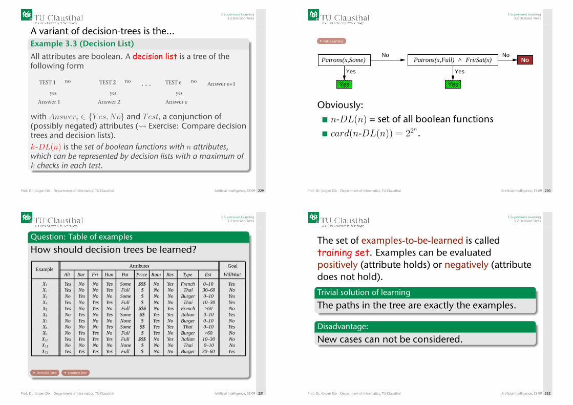
3 Supervised Learning3.2 Decision Trees
A variant of decision-trees is the...Example 3.3 (Decision List)
All attributes are boolean. A decision list is a tree of thefollowing form
yes
no Answer e+1
Answer e
TEST eTEST 2TEST 1
yes yes
no no
Answer 1 Answer 2
. . .
with Answeri ∈ {Y es,No} and Testi a conjunction of(possibly negated) attributes ( Exercise: Compare decisiontrees and decision lists).k-DL(n) is the set of boolean functions with n attributes,which can be represented by decision lists with a maximum ofk checks in each test.
Prof. Dr. Jürgen Dix · Department of Informatics, TU Clausthal Artificial Intelligence, SS 09 229
3 Supervised Learning3.2 Decision Trees
PAC-Learning
Patrons(x,Some)No
Yes Yes
No
>Patrons(x,Full) Fri/Sat(x)
Yes
No
Yes
Obviously:n-DL(n) = set of all boolean functionscard(n-DL(n)) = 22n.
Prof. Dr. Jürgen Dix · Department of Informatics, TU Clausthal Artificial Intelligence, SS 09 230
3 Supervised Learning3.2 Decision Trees
Question: Table of examples
How should decision trees be learned?
ExampleAttributes Goal
Alt Bar Fri Hun Pat Price Rain Res Type Est WillWait
X1 Yes No No Yes Some $$$ No Yes French 0–10 YesX2 Yes No No Yes Full $ No No Thai 30–60 NoX3 No Yes No No Some $ No No Burger 0–10 YesX4 Yes No Yes Yes Full $ No No Thai 10–30 YesX5 Yes No Yes No Full $$$ No Yes French >60 NoX6 No Yes No Yes Some $$ Yes Yes Italian 0–10 YesX7 No Yes No No None $ Yes No Burger 0–10 NoX8 No No No Yes Some $$ Yes Yes Thai 0–10 YesX9 No Yes Yes No Full $ Yes No Burger >60 NoX10 Yes Yes Yes Yes Full $$$ No Yes Italian 10–30 NoX11 No No No No None $ No No Thai 0–10 NoX12 Yes Yes Yes Yes Full $ No No Burger 30–60 Yes
Decision Tree Learned Tree
Prof. Dr. Jürgen Dix · Department of Informatics, TU Clausthal Artificial Intelligence, SS 09 231
3 Supervised Learning3.2 Decision Trees
The set of examples-to-be-learned is calledtraining set. Examples can be evaluatedpositively (attribute holds) or negatively (attributedoes not hold).
Trivial solution of learning
The paths in the tree are exactly the examples.
Disadvantage:
New cases can not be considered.
Prof. Dr. Jürgen Dix · Department of Informatics, TU Clausthal Artificial Intelligence, SS 09 232
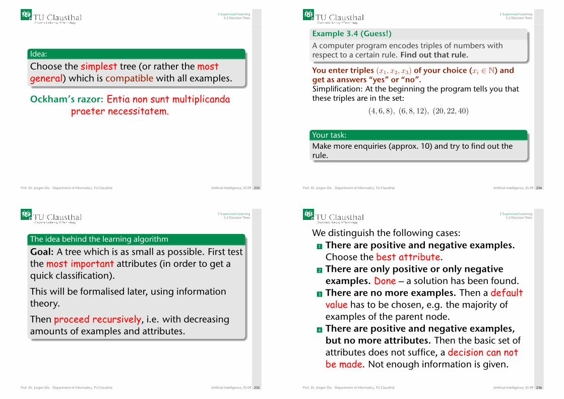
3 Supervised Learning3.2 Decision Trees
Idea:
Choose the simplest tree (or rather the mostgeneral) which is compatible with all examples.
Ockham’s razor: Entia non sunt multiplicandapraeter necessitatem.
Prof. Dr. Jürgen Dix · Department of Informatics, TU Clausthal Artificial Intelligence, SS 09 233
3 Supervised Learning3.2 Decision Trees
Example 3.4 (Guess!)A computer program encodes triples of numbers withrespect to a certain rule. Find out that rule.
You enter triples (x1, x2, x3) of your choice (xi ∈ N) andget as answers “yes” or “no”.Simplification: At the beginning the program tells you thatthese triples are in the set:
(4, 6, 8), (6, 8, 12), (20, 22, 40)
Your task:Make more enquiries (approx. 10) and try to find out therule.
Prof. Dr. Jürgen Dix · Department of Informatics, TU Clausthal Artificial Intelligence, SS 09 234
3 Supervised Learning3.2 Decision Trees
The idea behind the learning algorithm
Goal: A tree which is as small as possible. First testthe most important attributes (in order to get aquick classification).
This will be formalised later, using informationtheory.
Then proceed recursively, i.e. with decreasingamounts of examples and attributes.
Prof. Dr. Jürgen Dix · Department of Informatics, TU Clausthal Artificial Intelligence, SS 09 235
3 Supervised Learning3.2 Decision Trees
We distinguish the following cases:1 There are positive and negative examples.
Choose the best attribute.2 There are only positive or only negative
examples. Done – a solution has been found.3 There are no more examples. Then a defaultvalue has to be chosen, e.g. the majority ofexamples of the parent node.
4 There are positive and negative examples,but no more attributes. Then the basic set ofattributes does not suffice, a decision can notbe made. Not enough information is given.
Prof. Dr. Jürgen Dix · Department of Informatics, TU Clausthal Artificial Intelligence, SS 09 236
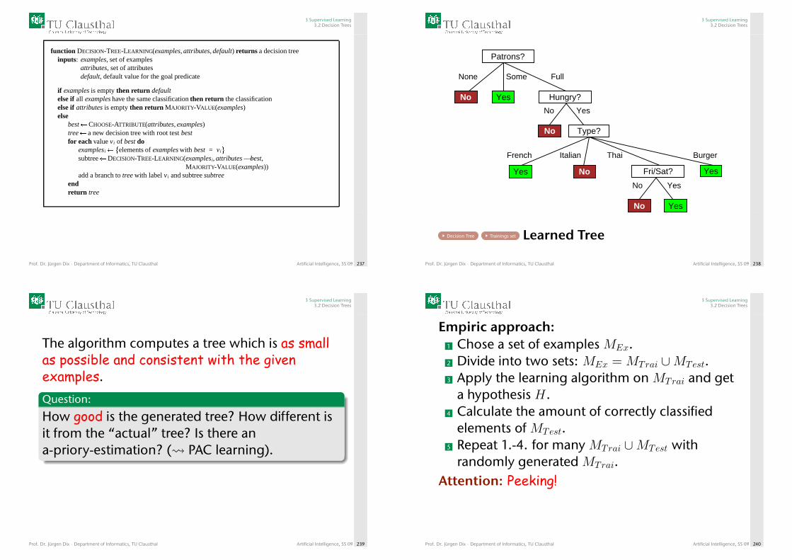
3 Supervised Learning3.2 Decision Trees
function DECISION-TREE-LEARNING(examples, attributes, default) returns a decision treeinputs: examples, set of examples
attributes, set of attributesdefault, default value for the goal predicate
if examples is empty then return defaultelse if all examples have the same classification then return the classificationelse if attributes is empty then return MAJORITY-VALUE(examples)else
best�CHOOSE-ATTRIBUTE(attributes, examples)tree� a new decision tree with root test bestfor each value vi of best do
examplesi�felements of examples with best = vigsubtree�DECISION-TREE-LEARNING(examplesi, attributes� best,
MAJORITY-VALUE(examples))add a branch to tree with label vi and subtree subtree
endreturn tree
Prof. Dr. Jürgen Dix · Department of Informatics, TU Clausthal Artificial Intelligence, SS 09 237
3 Supervised Learning3.2 Decision Trees
None Some Full
Patrons?
No Yes
No Yes
Hungry?
No
No Yes
Fri/Sat?
YesNo
Yes
Type?
French Italian Thai Burger
Yes No
Decision Tree Trainings set Learned Tree
Prof. Dr. Jürgen Dix · Department of Informatics, TU Clausthal Artificial Intelligence, SS 09 238
3 Supervised Learning3.2 Decision Trees
The algorithm computes a tree which is as smallas possible and consistent with the givenexamples.
Question:
How good is the generated tree? How different isit from the “actual” tree? Is there ana-priory-estimation? ( PAC learning).
Prof. Dr. Jürgen Dix · Department of Informatics, TU Clausthal Artificial Intelligence, SS 09 239
3 Supervised Learning3.2 Decision Trees
Empiric approach:1 Chose a set of examples MEx.2 Divide into two sets: MEx = MTrai ∪MTest.3 Apply the learning algorithm on MTrai and get
a hypothesis H.4 Calculate the amount of correctly classified
elements of MTest.5 Repeat 1.-4. for many MTrai ∪MTest with
randomly generated MTrai.Attention: Peeking!
Prof. Dr. Jürgen Dix · Department of Informatics, TU Clausthal Artificial Intelligence, SS 09 240
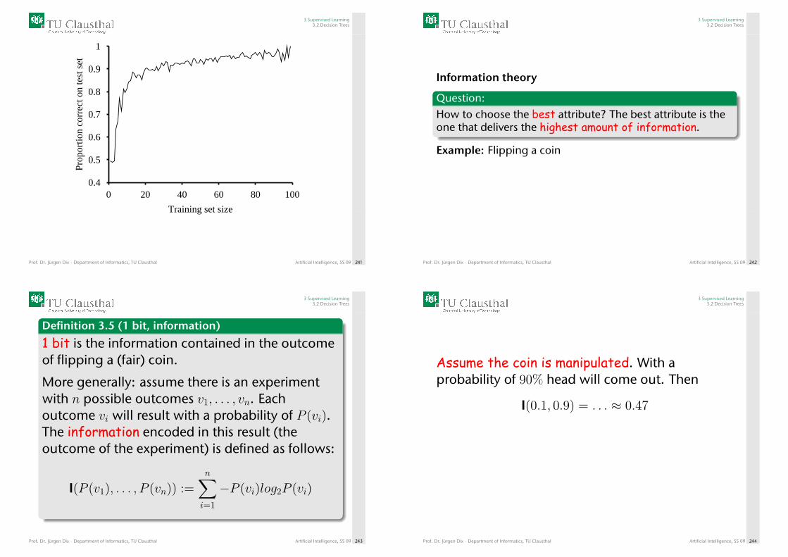
3 Supervised Learning3.2 Decision Trees
0.4
0.5
0.6
0.7
0.8
0.9
1
0 20 40 60 80 100
Prop
ortio
n co
rrec
t on
test
set
Training set size
Prof. Dr. Jürgen Dix · Department of Informatics, TU Clausthal Artificial Intelligence, SS 09 241
3 Supervised Learning3.2 Decision Trees
Information theory
Question:How to choose the best attribute? The best attribute is theone that delivers the highest amount of information.
Example: Flipping a coin
Prof. Dr. Jürgen Dix · Department of Informatics, TU Clausthal Artificial Intelligence, SS 09 242
3 Supervised Learning3.2 Decision Trees
Definition 3.5 (1 bit, information)
1 bit is the information contained in the outcomeof flipping a (fair) coin.
More generally: assume there is an experimentwith n possible outcomes v1, . . . , vn. Eachoutcome vi will result with a probability of P (vi).The information encoded in this result (theoutcome of the experiment) is defined as follows:
I(P (v1), . . . , P (vn)) :=n∑i=1
−P (vi)log2P (vi)
Prof. Dr. Jürgen Dix · Department of Informatics, TU Clausthal Artificial Intelligence, SS 09 243
3 Supervised Learning3.2 Decision Trees
Assume the coin is manipulated. With aprobability of 90% head will come out. Then
I(0.1, 0.9) = . . . ≈ 0.47
Prof. Dr. Jürgen Dix · Department of Informatics, TU Clausthal Artificial Intelligence, SS 09 244
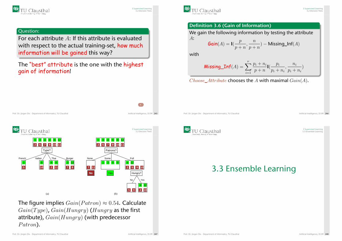
3 Supervised Learning3.2 Decision Trees
Question:
For each attribute A: If this attribute is evaluatedwith respect to the actual training-set, how muchinformation will be gained this way?
The “best” attribute is the one with the highestgain of information!
Prof. Dr. Jürgen Dix · Department of Informatics, TU Clausthal Artificial Intelligence, SS 09 245
3 Supervised Learning3.2 Decision Trees
Definition 3.6 (Gain of Information)We gain the following information by testing the attributeA:
Gain(A) = I(p
p+ n,
n
p+ n)−Missing_Inf(A)
with
Missing_Inf(A) =ν∑i=1
pi + nip+ n
I(pi
pi + ni,
nipi + ni
)
Choose_Attribute chooses the A with maximal Gain(A).
Prof. Dr. Jürgen Dix · Department of Informatics, TU Clausthal Artificial Intelligence, SS 09 246
3 Supervised Learning3.2 Decision Trees
(a)
French Italian Thai Burger
Type?
None Some Full
Patrons?
YesNo Hungry?
(b)
No Yes
121 3 4 6 8
2 5 7 9 10 11
121 3 4 6 8
2 5 7 9 10 11
1
5
6
10
4 8
2 11
123
7 9 7 11
1 3 6 8 124
2 5 9 10
124
2 105 9
The figure implies Gain(Patron) ≈ 0.54. CalculateGain(Type), Gain(Hungry) (Hungry as the firstattribute), Gain(Hungry) (with predecessorPatron).
Prof. Dr. Jürgen Dix · Department of Informatics, TU Clausthal Artificial Intelligence, SS 09 247
3 Supervised Learning3.3 Ensemble Learning
3.3 Ensemble Learning
Prof. Dr. Jürgen Dix · Department of Informatics, TU Clausthal Artificial Intelligence, SS 09 248
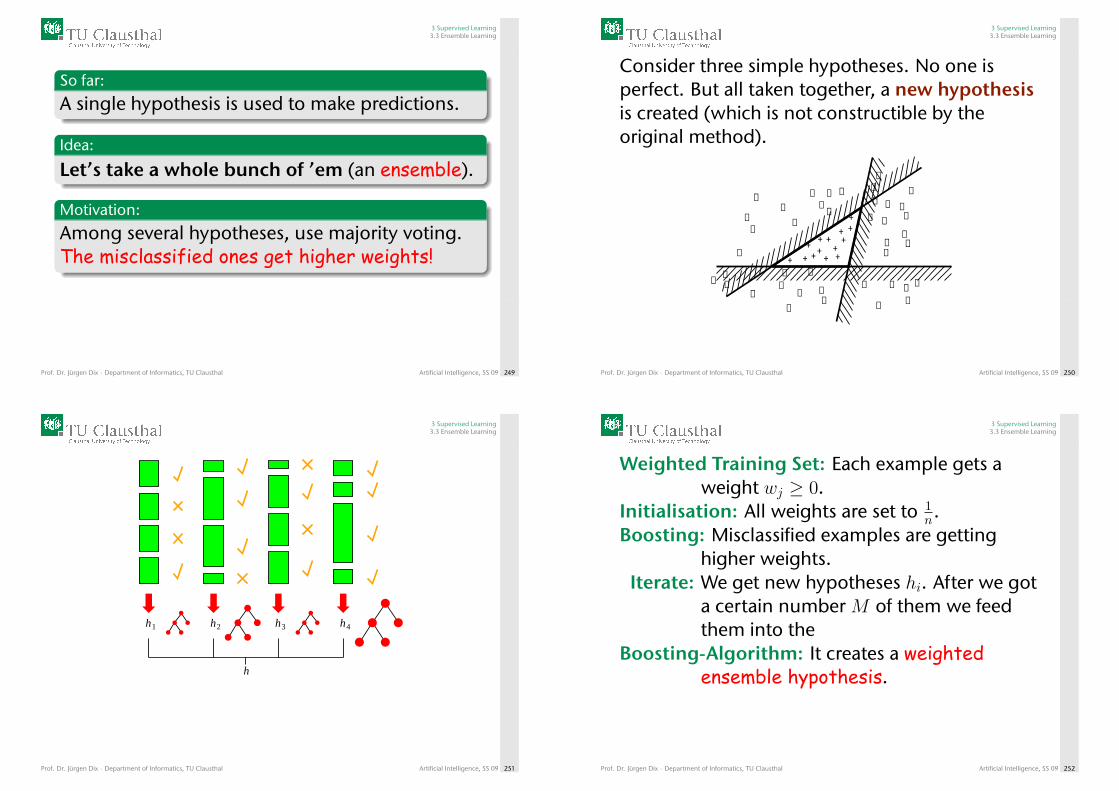
3 Supervised Learning3.3 Ensemble Learning
So far:
A single hypothesis is used to make predictions.
Idea:
Let’s take a whole bunch of ’em (an ensemble).
Motivation:
Among several hypotheses, use majority voting.The misclassified ones get higher weights!
Prof. Dr. Jürgen Dix · Department of Informatics, TU Clausthal Artificial Intelligence, SS 09 249
3 Supervised Learning3.3 Ensemble Learning
Consider three simple hypotheses. No one isperfect. But all taken together, a new hypothesisis created (which is not constructible by theoriginal method).
++
++
++++++
++
++
−−−−
−
−−
−
−−
−−
−−
−
−−
− − −−
− −−−
− −
−−
−−
−
−− −
−
−− −
−
−
Prof. Dr. Jürgen Dix · Department of Informatics, TU Clausthal Artificial Intelligence, SS 09 250
3 Supervised Learning3.3 Ensemble Learning
h1 h2 h3 h4
h
Prof. Dr. Jürgen Dix · Department of Informatics, TU Clausthal Artificial Intelligence, SS 09 251
3 Supervised Learning3.3 Ensemble Learning
Weighted Training Set: Each example gets aweight wj ≥ 0.
Initialisation: All weights are set to 1n.
Boosting: Misclassified examples are gettinghigher weights.
Iterate: We get new hypotheses hi. After we gota certain number M of them we feedthem into the
Boosting-Algorithm: It creates a weightedensemble hypothesis.
Prof. Dr. Jürgen Dix · Department of Informatics, TU Clausthal Artificial Intelligence, SS 09 252
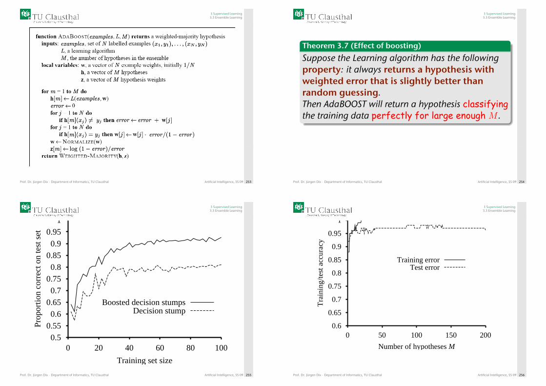
3 Supervised Learning3.3 Ensemble Learning
Prof. Dr. Jürgen Dix · Department of Informatics, TU Clausthal Artificial Intelligence, SS 09 253
3 Supervised Learning3.3 Ensemble Learning
Theorem 3.7 (Effect of boosting)
Suppose the Learning algorithm has the followingproperty: it always returns a hypothesis withweighted error that is slightly better thanrandom guessing.Then AdaBOOST will return a hypothesis classifyingthe training data perfectly for large enough M .
Prof. Dr. Jürgen Dix · Department of Informatics, TU Clausthal Artificial Intelligence, SS 09 254
3 Supervised Learning3.3 Ensemble Learning
0.50.55
0.60.65
0.70.750.8
0.850.9
0.951
0 20 40 60 80 100
Prop
ortio
n co
rrec
t on
test
set
Training set size
Boosted decision stumpsDecision stump
Prof. Dr. Jürgen Dix · Department of Informatics, TU Clausthal Artificial Intelligence, SS 09 255
3 Supervised Learning3.3 Ensemble Learning
0.6
0.65
0.7
0.75
0.8
0.85
0.9
0.95
1
0 50 100 150 200
Tra
inin
g/te
st a
ccur
acy
Number of hypotheses M
Training errorTest error
Prof. Dr. Jürgen Dix · Department of Informatics, TU Clausthal Artificial Intelligence, SS 09 256
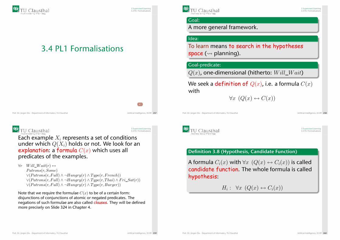
3 Supervised Learning3.4 PL1 Formalisations
3.4 PL1 Formalisations
Prof. Dr. Jürgen Dix · Department of Informatics, TU Clausthal Artificial Intelligence, SS 09 257
3 Supervised Learning3.4 PL1 Formalisations
Goal:
A more general framework.
Idea:
To learn means to search in the hypothesesspace ( planning).
Goal-predicate:
Q(x), one-dimensional (hitherto: Will_Wait)
We seek a definition of Q(x), i.e. a formula C(x)with
∀x (Q(x)↔ C(x))
Prof. Dr. Jürgen Dix · Department of Informatics, TU Clausthal Artificial Intelligence, SS 09 258
3 Supervised Learning3.4 PL1 Formalisations
Each example Xi represents a set of conditionsunder which Q(Xi) holds or not. We look for anexplanation: a formula C(x) which uses allpredicates of the examples.∀r Will_Wait(r)↔
Patrons(r, Some)∨(Patrons(r, Full) ∧ ¬Hungry(r) ∧ Type(r, French))∨(Patrons(r, Full) ∧ ¬Hungry(r) ∧ Type(r, Thai) ∧ Fri_Sat(r))∨(Patrons(r, Full) ∧ ¬Hungry(r) ∧ Type(r,Burger))
Note that we require the formulae C(x) to be of a certain form:disjunctions of conjunctions of atomic or negated predicates. Thenegations of such formulae are also called clauses. They will be definedmore precisely on Slide 324 in Chapter 4.
Prof. Dr. Jürgen Dix · Department of Informatics, TU Clausthal Artificial Intelligence, SS 09 259
3 Supervised Learning3.4 PL1 Formalisations
Definition 3.8 (Hypothesis, Candidate Function)
A formula Ci(x) with ∀x (Q(x)↔ Ci(x)) is calledcandidate function. The whole formula is calledhypothesis:
Hi : ∀x (Q(x)↔ Ci(x))
Prof. Dr. Jürgen Dix · Department of Informatics, TU Clausthal Artificial Intelligence, SS 09 260
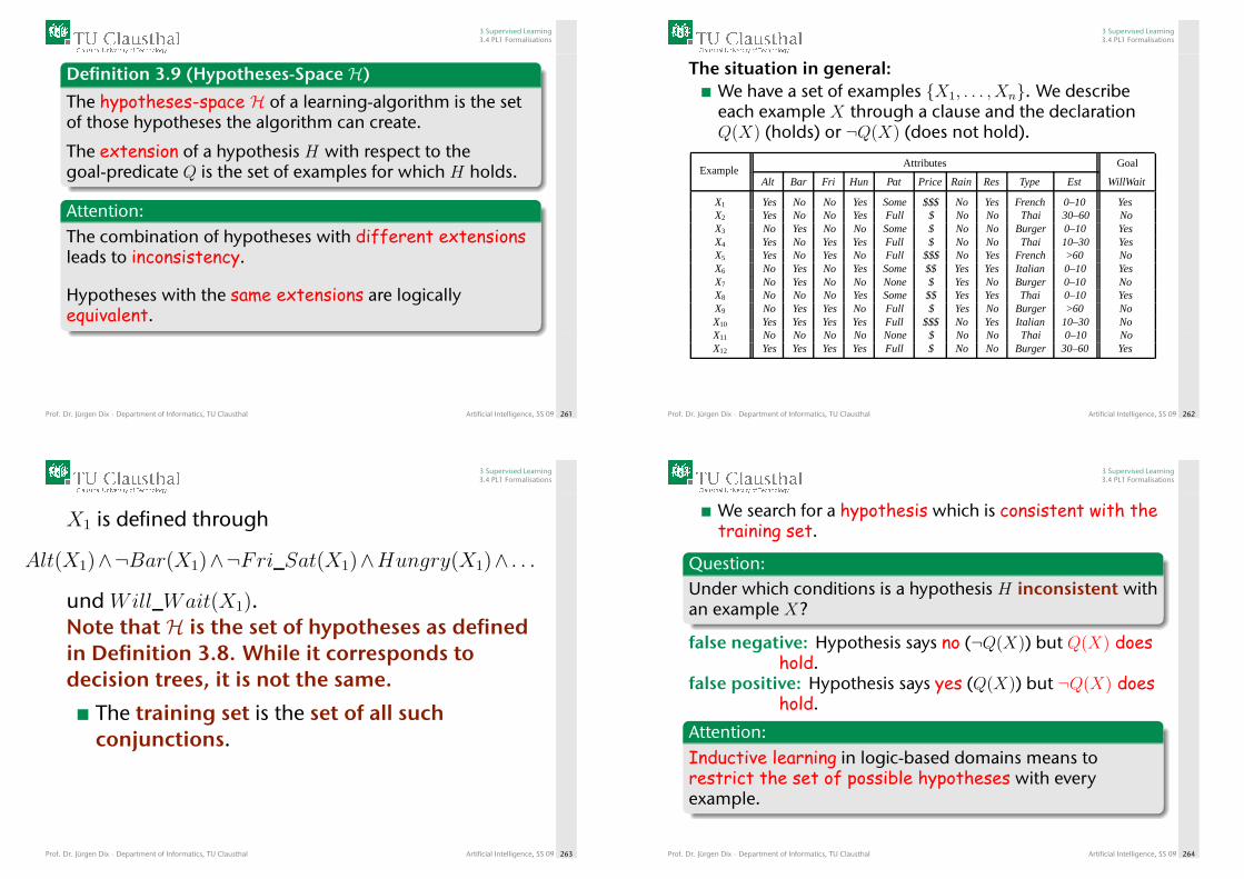
3 Supervised Learning3.4 PL1 Formalisations
Definition 3.9 (Hypotheses-Space H)
The hypotheses-space H of a learning-algorithm is the setof those hypotheses the algorithm can create.
The extension of a hypothesis H with respect to thegoal-predicate Q is the set of examples for which H holds.
Attention:The combination of hypotheses with different extensionsleads to inconsistency.
Hypotheses with the same extensions are logicallyequivalent.
Prof. Dr. Jürgen Dix · Department of Informatics, TU Clausthal Artificial Intelligence, SS 09 261
3 Supervised Learning3.4 PL1 Formalisations
The situation in general:We have a set of examples {X1, . . . , Xn}. We describeeach example X through a clause and the declarationQ(X) (holds) or ¬Q(X) (does not hold).
ExampleAttributes Goal
Alt Bar Fri Hun Pat Price Rain Res Type Est WillWait
X1 Yes No No Yes Some $$$ No Yes French 0–10 YesX2 Yes No No Yes Full $ No No Thai 30–60 NoX3 No Yes No No Some $ No No Burger 0–10 YesX4 Yes No Yes Yes Full $ No No Thai 10–30 YesX5 Yes No Yes No Full $$$ No Yes French >60 NoX6 No Yes No Yes Some $$ Yes Yes Italian 0–10 YesX7 No Yes No No None $ Yes No Burger 0–10 NoX8 No No No Yes Some $$ Yes Yes Thai 0–10 YesX9 No Yes Yes No Full $ Yes No Burger >60 NoX10 Yes Yes Yes Yes Full $$$ No Yes Italian 10–30 NoX11 No No No No None $ No No Thai 0–10 NoX12 Yes Yes Yes Yes Full $ No No Burger 30–60 Yes
Prof. Dr. Jürgen Dix · Department of Informatics, TU Clausthal Artificial Intelligence, SS 09 262
3 Supervised Learning3.4 PL1 Formalisations
X1 is defined through
Alt(X1)∧¬Bar(X1)∧¬Fri_Sat(X1)∧Hungry(X1)∧ . . .
und Will_Wait(X1).Note that H is the set of hypotheses as definedin Definition 3.8. While it corresponds todecision trees, it is not the same.
The training set is the set of all suchconjunctions.
Prof. Dr. Jürgen Dix · Department of Informatics, TU Clausthal Artificial Intelligence, SS 09 263
3 Supervised Learning3.4 PL1 Formalisations
We search for a hypothesis which is consistent with thetraining set.
Question:Under which conditions is a hypothesis H inconsistent withan example X?
false negative: Hypothesis says no (¬Q(X)) but Q(X) doeshold.
false positive: Hypothesis says yes (Q(X)) but ¬Q(X) doeshold.
Attention:Inductive learning in logic-based domains means torestrict the set of possible hypotheses with everyexample.
Prof. Dr. Jürgen Dix · Department of Informatics, TU Clausthal Artificial Intelligence, SS 09 264
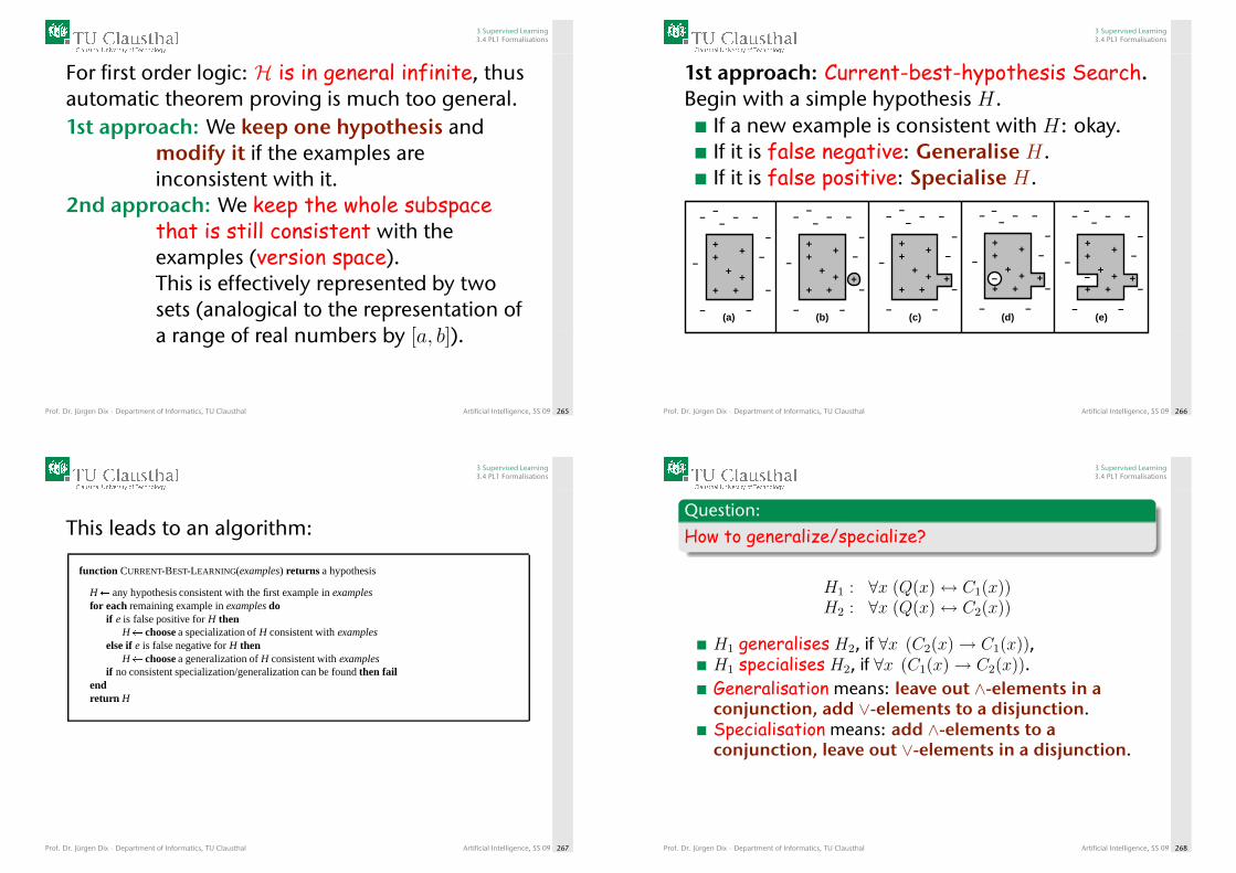
3 Supervised Learning3.4 PL1 Formalisations
For first order logic: H is in general infinite, thusautomatic theorem proving is much too general.1st approach: We keep one hypothesis and
modify it if the examples areinconsistent with it.
2nd approach: We keep the whole subspacethat is still consistent with theexamples (version space).This is effectively represented by twosets (analogical to the representation ofa range of real numbers by [a, b]).
Prof. Dr. Jürgen Dix · Department of Informatics, TU Clausthal Artificial Intelligence, SS 09 265
3 Supervised Learning3.4 PL1 Formalisations
1st approach: Current-best-hypothesis Search.Begin with a simple hypothesis H.
If a new example is consistent with H: okay.If it is false negative: Generalise H.If it is false positive: Specialise H.
(a) (b) (c) (d) (e)
++
+
++
+ +
−−
−
−
−−
−
− −−
−
++
+
++
+ +
−−
−
−
−−
−
− −−
−
+
++
+
++
+ +
−−
−
−
−−
−
− −−
−
+
++
+
++
+ +
−−
−
−
−−
−
− −
−
+−
++
+
++
+ +
−−
−
−
−−
−
− −
−
+
− −
−
Prof. Dr. Jürgen Dix · Department of Informatics, TU Clausthal Artificial Intelligence, SS 09 266
3 Supervised Learning3.4 PL1 Formalisations
This leads to an algorithm:
function CURRENT-BEST-LEARNING(examples) returns a hypothesis
H� any hypothesis consistent with the first example in examplesfor each remaining example in examples do
if e is false positive for H thenH� choose a specialization of H consistent with examples
else if e is false negative for H thenH� choose a generalization of H consistent with examples
if no consistent specialization/generalization can be found then failendreturn H
Prof. Dr. Jürgen Dix · Department of Informatics, TU Clausthal Artificial Intelligence, SS 09 267
3 Supervised Learning3.4 PL1 Formalisations
Question:
How to generalize/specialize?
H1 : ∀x (Q(x)↔ C1(x))H2 : ∀x (Q(x)↔ C2(x))
H1 generalises H2, if ∀x (C2(x)→ C1(x)),H1 specialises H2, if ∀x (C1(x)→ C2(x)).Generalisation means: leave out ∧-elements in aconjunction, add ∨-elements to a disjunction.Specialisation means: add ∧-elements to aconjunction, leave out ∨-elements in a disjunction.
Prof. Dr. Jürgen Dix · Department of Informatics, TU Clausthal Artificial Intelligence, SS 09 268
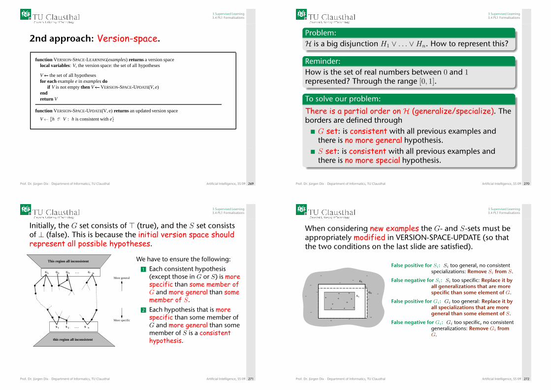
3 Supervised Learning3.4 PL1 Formalisations
2nd approach: Version-space.
function VERSION-SPACE-LEARNING(examples) returns a version spacelocal variables: V, the version space: the set of all hypotheses
V� the set of all hypothesesfor each example e in examples do
if V is not empty then V�VERSION-SPACE-UPDATE(V, e)endreturn V
function VERSION-SPACE-UPDATE(V, e) returns an updated version space
V�fh � V : h is consistent with eg
Prof. Dr. Jürgen Dix · Department of Informatics, TU Clausthal Artificial Intelligence, SS 09 269
3 Supervised Learning3.4 PL1 Formalisations
Problem:H is a big disjunction H1 ∨ . . . ∨Hn. How to represent this?
Reminder:How is the set of real numbers between 0 and 1represented? Through the range [0, 1].
To solve our problem:
There is a partial order on H (generalize/specialize). Theborders are defined through
G set: is consistent with all previous examples andthere is no more general hypothesis.S set: is consistent with all previous examples andthere is no more special hypothesis.
Prof. Dr. Jürgen Dix · Department of Informatics, TU Clausthal Artificial Intelligence, SS 09 270
3 Supervised Learning3.4 PL1 Formalisations
Initially, the G set consists of > (true), and the S set consistsof ⊥ (false). This is because the initial version space shouldrepresent all possible hypotheses.
this region all inconsistent
This region all inconsistent
More general
More specific
S 1
G1
S 2
G2 G3 . . . G m
. . . S n
We have to ensure the following:1 Each consistent hypothesis
(except those in G or S) is morespecific than some member ofG and more general than somemember of S.
2 Each hypothesis that is morespecific than some member ofG and more general than somemember of S is a consistenthypothesis.
Prof. Dr. Jürgen Dix · Department of Informatics, TU Clausthal Artificial Intelligence, SS 09 271
3 Supervised Learning3.4 PL1 Formalisations
When considering new examples the G- and S-sets must beappropriately modified in VERSION-SPACE-UPDATE (so thatthe two conditions on the last slide are satisfied).
+ +
+ +
+
+
++
+ +
−
−
−
−
−
−−
−
− −−
−−
−
S 1
1G
G2
False positive for Si: Si too general, no consistentspecializations: Remove Si from S.
False negative for Si: Si too specific: Replace it byall generalizations that are morespecific than some element of G.
False positive for Gi: Gi too general: Replace it byall specializations that are moregeneral than some element of S.
False negative for Gi: Gi too specific, no consistentgeneralizations: Remove Gi fromG.
Prof. Dr. Jürgen Dix · Department of Informatics, TU Clausthal Artificial Intelligence, SS 09 272
3 Supervised Learning3.4 PL1 Formalisations
Question:
What can happen?
We iterate the algorithm on the previous slideuntil one of the following happens:
1 Only one hypothesis remains: That is oursolution!
2 The space collapses: There is no consistenthypothesis, G = ∅ or S = ∅.
3 No examples are left, but there are still severalhypotheses: Result is a big disjunction.
Prof. Dr. Jürgen Dix · Department of Informatics, TU Clausthal Artificial Intelligence, SS 09 273
4 Knowledge Engineering (1)
4. Knowledge Engineering (1)4 Knowledge Engineering (1)
Sentential LogicSudokuCalculi for SLWumpus in SLA Puzzle
Prof. Dr. Jürgen Dix · Department of Informatics, TU Clausthal Artificial Intelligence, SS 09 274
4 Knowledge Engineering (1)
Content of this chapter (1):
Logic: We introduce sentential logic (also calledpropositional logic). This logic dates back toBoole and is the basis for many logicalframeworks. The essential features of mostlogics can be illustrated in a puristic way.We are using logics to describe the world andhow the world behaves.
Sudoku: We illustrate how to use SL with the game ofSudoku. The conditions of being a solution canbe easily stated in SL.
Prof. Dr. Jürgen Dix · Department of Informatics, TU Clausthal Artificial Intelligence, SS 09 275
4 Knowledge Engineering (1)
Content of this chapter (2):
Calculi for SL: While it is nice to describe the world, or thesolution of a Sudoku puzzle, we also want todraw conclusions about it or even to solve thepuzzle. Therefore we have to derive newinformation and deduce statements, that are notexplicitly given.
Examples: We illustrate the use of SL with two moreexamples: The Wumpus world and one of theweekly puzzles in the newspaper Die Zeit.
Prof. Dr. Jürgen Dix · Department of Informatics, TU Clausthal Artificial Intelligence, SS 09 276
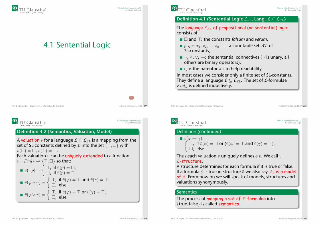
4 Knowledge Engineering (1)4.1 Sentential Logic
4.1 Sentential Logic
Prof. Dr. Jürgen Dix · Department of Informatics, TU Clausthal Artificial Intelligence, SS 09 277
4 Knowledge Engineering (1)4.1 Sentential Logic
Definition 4.1 (Sentential Logic LSL, Lang. L ⊆ LSL)
The language LSL of propositional (or sentential) logicconsists of� and >: the constants falsum and verum,p, q, r, x1, x2, . . . xn, . . .: a countable set AT ofSL-constants,¬, ∧, ∨,→: the sentential connectives (¬ is unary, allothers are binary operators),(, ): the parentheses to help readability.
In most cases we consider only a finite set of SL-constants.They define a language L ⊆ LSL. The set of L-formulaeFmlL is defined inductively.
Prof. Dr. Jürgen Dix · Department of Informatics, TU Clausthal Artificial Intelligence, SS 09 278
4 Knowledge Engineering (1)4.1 Sentential Logic
Definition 4.2 (Semantics, Valuation, Model)
A valuation v for a language L ⊆ LSL is a mapping from theset of SL-constants defined by L into the set {>,�} withv(�) = �, v(>) = >.Each valuation v can be uniquely extended to a functionv̄ : FmlL → {>,�} so that:
v̄(¬p) =
{>, if v̄(p) = �,�, if v̄(p) = >.
v̄(ϕ ∧ γ) =
{>, if v̄(ϕ) = > and v̄(γ) = >,�, else
v̄(ϕ ∨ γ) =
{>, if v̄(ϕ) = > or v̄(γ) = >,�, else
Prof. Dr. Jürgen Dix · Department of Informatics, TU Clausthal Artificial Intelligence, SS 09 279
4 Knowledge Engineering (1)4.1 Sentential Logic
Definition (continued)v̄(ϕ→ γ) ={>, if v̄(ϕ) = � or (v̄(ϕ) = > and v̄(γ) = >),�, else
Thus each valuation v uniquely defines a v̄. We call v̄L-structure.A structure determines for each formula if it is true or false.If a formula φ is true in structure v̄ we also say Av is a modelof φ. From now on we will speak of models, structures andvaluations synonymously.
SemanticsThe process of mapping a set of L-formulae into{true, false} is called semantics.
Prof. Dr. Jürgen Dix · Department of Informatics, TU Clausthal Artificial Intelligence, SS 09 280
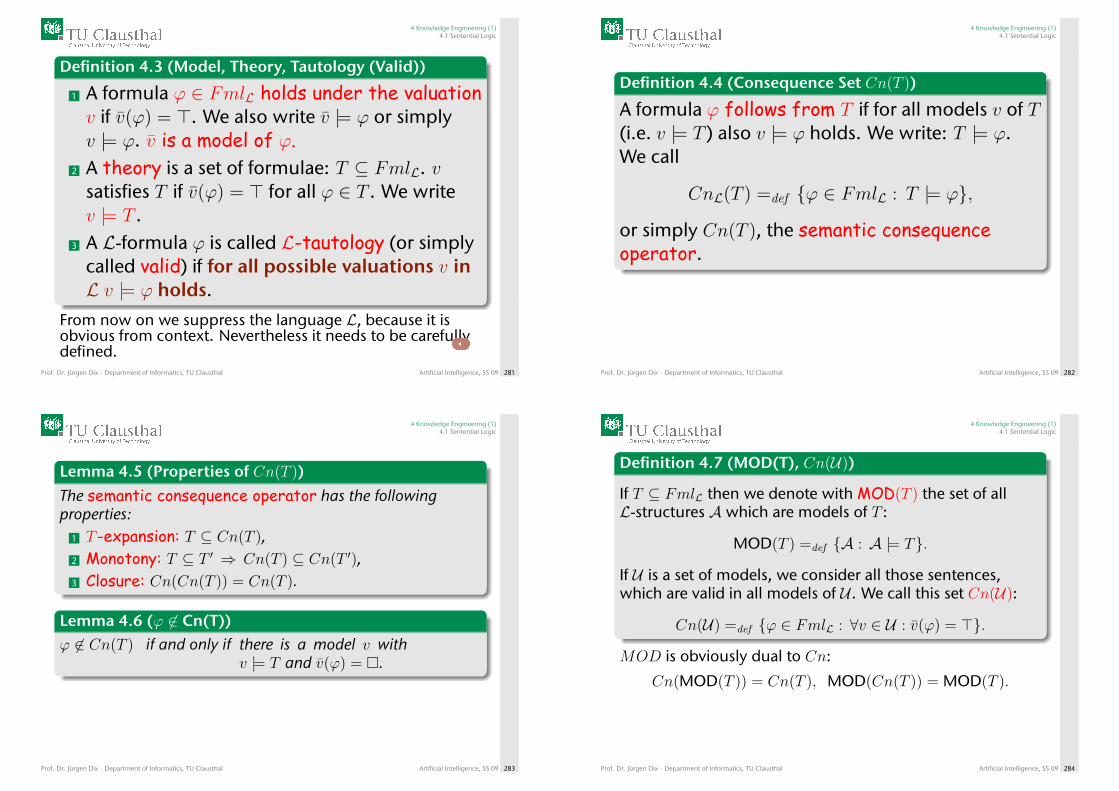
4 Knowledge Engineering (1)4.1 Sentential Logic
Definition 4.3 (Model, Theory, Tautology (Valid))
1 A formula ϕ ∈ FmlL holds under the valuationv if v̄(ϕ) = >. We also write v̄ |= ϕ or simplyv |= ϕ. v̄ is a model of ϕ.
2 A theory is a set of formulae: T ⊆ FmlL. vsatisfies T if v̄(ϕ) = > for all ϕ ∈ T . We writev |= T .
3 A L-formula ϕ is called L-tautology (or simplycalled valid) if for all possible valuations v inL v |= ϕ holds.
From now on we suppress the language L, because it isobvious from context. Nevertheless it needs to be carefullydefined.
Prof. Dr. Jürgen Dix · Department of Informatics, TU Clausthal Artificial Intelligence, SS 09 281
4 Knowledge Engineering (1)4.1 Sentential Logic
Definition 4.4 (Consequence Set Cn(T ))
A formula ϕ follows from T if for all models v of T(i.e. v |= T ) also v |= ϕ holds. We write: T |= ϕ.We call
CnL(T ) =def {ϕ ∈ FmlL : T |= ϕ},
or simply Cn(T ), the semantic consequenceoperator.
Prof. Dr. Jürgen Dix · Department of Informatics, TU Clausthal Artificial Intelligence, SS 09 282
4 Knowledge Engineering (1)4.1 Sentential Logic
Lemma 4.5 (Properties of Cn(T ))
The semantic consequence operator has the followingproperties:
1 T -expansion: T ⊆ Cn(T ),2 Monotony: T ⊆ T ′ ⇒ Cn(T ) ⊆ Cn(T ′),3 Closure: Cn(Cn(T )) = Cn(T ).
Lemma 4.6 (ϕ 6∈ Cn(T))ϕ 6∈ Cn(T ) if and only if there is a model v with
v |= T and v̄(ϕ) = �.
Prof. Dr. Jürgen Dix · Department of Informatics, TU Clausthal Artificial Intelligence, SS 09 283
4 Knowledge Engineering (1)4.1 Sentential Logic
Definition 4.7 (MOD(T), Cn(U))
If T ⊆ FmlL then we denote with MOD(T ) the set of allL-structures A which are models of T :
MOD(T ) =def {A : A |= T}.
If U is a set of models, we consider all those sentences,which are valid in all models of U . We call this set Cn(U):
Cn(U) =def {ϕ ∈ FmlL : ∀v ∈ U : v̄(ϕ) = >}.
MOD is obviously dual to Cn:
Cn(MOD(T )) = Cn(T ), MOD(Cn(T )) = MOD(T ).
Prof. Dr. Jürgen Dix · Department of Informatics, TU Clausthal Artificial Intelligence, SS 09 284
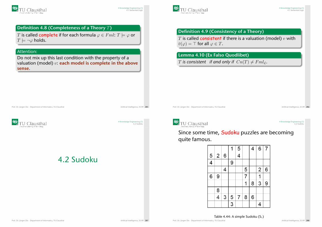
4 Knowledge Engineering (1)4.1 Sentential Logic
Definition 4.8 (Completeness of a Theory T )
T is called complete if for each formula ϕ ∈ Fml: T |= ϕ orT |= ¬ϕ holds.
Attention:Do not mix up this last condition with the property of avaluation (model) v: each model is complete in the abovesense.
Prof. Dr. Jürgen Dix · Department of Informatics, TU Clausthal Artificial Intelligence, SS 09 285
4 Knowledge Engineering (1)4.1 Sentential Logic
Definition 4.9 (Consistency of a Theory)
T is called consistent if there is a valuation (model) v withv̄(ϕ) = > for all ϕ ∈ T .
Lemma 4.10 (Ex Falso Quodlibet)T is consistent if and only if Cn(T ) 6= FmlL.
Prof. Dr. Jürgen Dix · Department of Informatics, TU Clausthal Artificial Intelligence, SS 09 286
4 Knowledge Engineering (1)4.2 Sudoku
4.2 Sudoku
Prof. Dr. Jürgen Dix · Department of Informatics, TU Clausthal Artificial Intelligence, SS 09 287
4 Knowledge Engineering (1)4.2 Sudoku
Since some time, Sudoku puzzles are becomingquite famous.
Table 4.44: A simple Sudoku (S1)Prof. Dr. Jürgen Dix · Department of Informatics, TU Clausthal Artificial Intelligence, SS 09 288
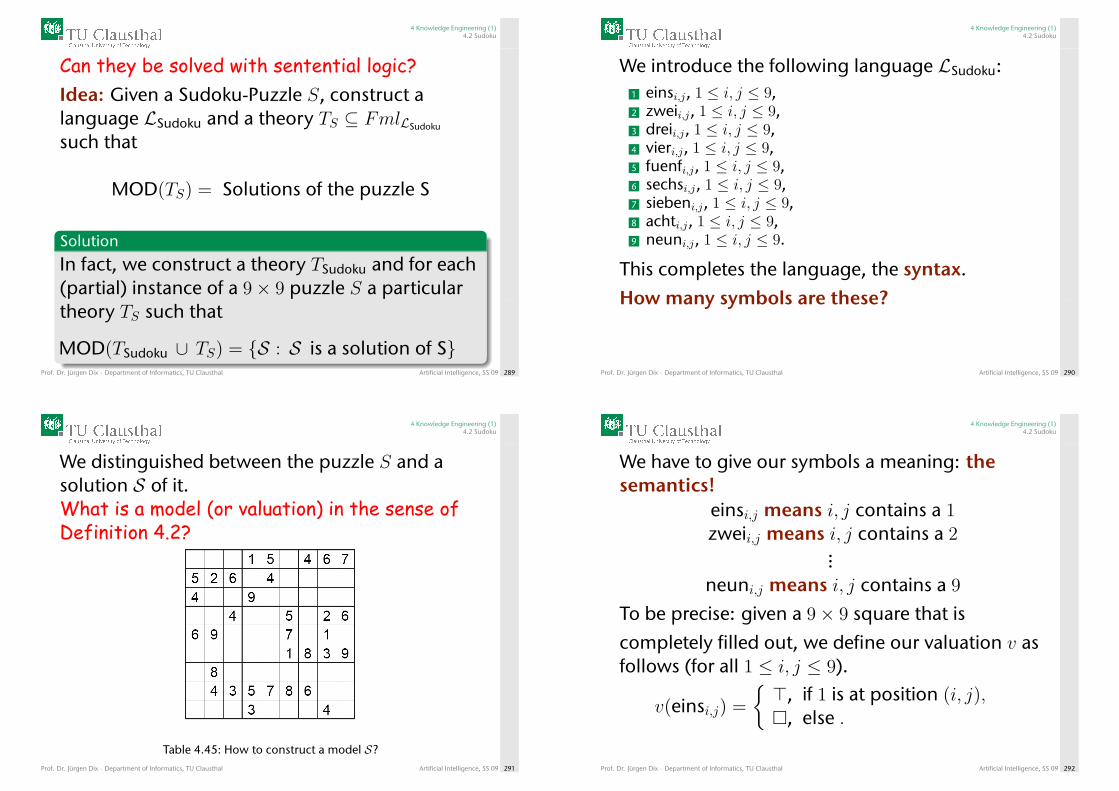
4 Knowledge Engineering (1)4.2 Sudoku
Can they be solved with sentential logic?Idea: Given a Sudoku-Puzzle S, construct alanguage LSudoku and a theory TS ⊆ FmlLSudoku
such that
MOD(TS) = Solutions of the puzzle S
Solution
In fact, we construct a theory TSudoku and for each(partial) instance of a 9× 9 puzzle S a particulartheory TS such that
MOD(TSudoku ∪ TS) = {S : S is a solution of S}Prof. Dr. Jürgen Dix · Department of Informatics, TU Clausthal Artificial Intelligence, SS 09 289
4 Knowledge Engineering (1)4.2 Sudoku
We introduce the following language LSudoku:1 einsi,j, 1 ≤ i, j ≤ 9,2 zweii,j, 1 ≤ i, j ≤ 9,3 dreii,j, 1 ≤ i, j ≤ 9,4 vieri,j, 1 ≤ i, j ≤ 9,5 fuenfi,j, 1 ≤ i, j ≤ 9,6 sechsi,j, 1 ≤ i, j ≤ 9,7 siebeni,j, 1 ≤ i, j ≤ 9,8 achti,j, 1 ≤ i, j ≤ 9,9 neuni,j, 1 ≤ i, j ≤ 9.
This completes the language, the syntax.
How many symbols are these?
Prof. Dr. Jürgen Dix · Department of Informatics, TU Clausthal Artificial Intelligence, SS 09 290
4 Knowledge Engineering (1)4.2 Sudoku
We distinguished between the puzzle S and asolution S of it.What is a model (or valuation) in the sense ofDefinition 4.2?
Table 4.45: How to construct a model S?Prof. Dr. Jürgen Dix · Department of Informatics, TU Clausthal Artificial Intelligence, SS 09 291
4 Knowledge Engineering (1)4.2 Sudoku
We have to give our symbols a meaning: thesemantics!
einsi,j means i, j contains a 1zweii,j means i, j contains a 2
...neuni,j means i, j contains a 9
To be precise: given a 9× 9 square that is
completely filled out, we define our valuation v asfollows (for all 1 ≤ i, j ≤ 9).
v(einsi,j) =
{>, if 1 is at position (i, j),�, else .
Prof. Dr. Jürgen Dix · Department of Informatics, TU Clausthal Artificial Intelligence, SS 09 292
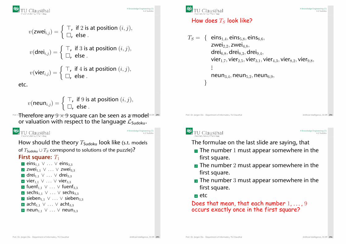
4 Knowledge Engineering (1)4.2 Sudoku
v(zweii,j) =
{>, if 2 is at position (i, j),�, else .
v(dreii,j) =
{>, if 3 is at position (i, j),�, else .
v(vieri,j) =
{>, if 4 is at position (i, j),�, else .
etc.
v(neuni,j) =
{>, if 9 is at position (i, j),�, else .
Therefore any 9× 9 square can be seen as a modelor valuation with respect to the language LSudoku.
Prof. Dr. Jürgen Dix · Department of Informatics, TU Clausthal Artificial Intelligence, SS 09 293
4 Knowledge Engineering (1)4.2 Sudoku
How does TS look like?
TS = { eins1,4, eins5,8, eins6,6,zwei2,2, zwei4,8,drei6,8,drei8,3,drei9,4,vier1,7, vier2,5, vier3,1, vier4,3, vier8,2, vier9,8,...neun3,4,neun5,2,neun6,9,
}
Prof. Dr. Jürgen Dix · Department of Informatics, TU Clausthal Artificial Intelligence, SS 09 294
4 Knowledge Engineering (1)4.2 Sudoku
How should the theory TSudoku look like (s.t. modelsof TSudoku ∪ TS correspond to solutions of the puzzle)?First square: T1
1 eins1,1 ∨ . . . ∨ eins3,3
2 zwei1,1 ∨ . . . ∨ zwei3,33 drei1,1 ∨ . . . ∨ drei3,34 vier1,1 ∨ . . . ∨ vier3,3
5 fuenf1,1 ∨ . . . ∨ fuenf3,36 sechs1,1 ∨ . . . ∨ sechs3,3
7 sieben1,1 ∨ . . . ∨ sieben3,3
8 acht1,1 ∨ . . . ∨ acht3,3
9 neun1,1 ∨ . . . ∨ neun3,3
Prof. Dr. Jürgen Dix · Department of Informatics, TU Clausthal Artificial Intelligence, SS 09 295
4 Knowledge Engineering (1)4.2 Sudoku
The formulae on the last slide are saying, that1 The number 1 must appear somewhere in the
first square.2 The number 2 must appear somewhere in the
first square.3 The number 3 must appear somewhere in the
first square.4 etc
Does that mean, that each number 1, . . . , 9occurs exactly once in the first square?
Prof. Dr. Jürgen Dix · Department of Informatics, TU Clausthal Artificial Intelligence, SS 09 296
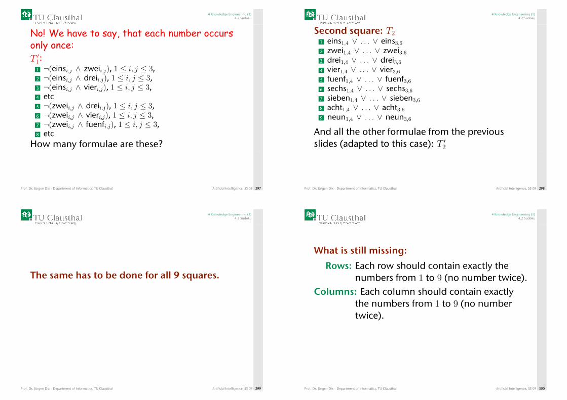
4 Knowledge Engineering (1)4.2 Sudoku
No! We have to say, that each number occursonly once:T ′1:
1 ¬(einsi,j ∧ zweii,j), 1 ≤ i, j ≤ 3,2 ¬(einsi,j ∧ dreii,j), 1 ≤ i, j ≤ 3,3 ¬(einsi,j ∧ vieri,j), 1 ≤ i, j ≤ 3,4 etc5 ¬(zweii,j ∧ dreii,j), 1 ≤ i, j ≤ 3,6 ¬(zweii,j ∧ vieri,j), 1 ≤ i, j ≤ 3,7 ¬(zweii,j ∧ fuenfi,j), 1 ≤ i, j ≤ 3,8 etc
How many formulae are these?
Prof. Dr. Jürgen Dix · Department of Informatics, TU Clausthal Artificial Intelligence, SS 09 297
4 Knowledge Engineering (1)4.2 Sudoku
Second square: T21 eins1,4 ∨ . . . ∨ eins3,6
2 zwei1,4 ∨ . . . ∨ zwei3,63 drei1,4 ∨ . . . ∨ drei3,64 vier1,4 ∨ . . . ∨ vier3,6
5 fuenf1,4 ∨ . . . ∨ fuenf3,66 sechs1,4 ∨ . . . ∨ sechs3,6
7 sieben1,4 ∨ . . . ∨ sieben3,6
8 acht1,4 ∨ . . . ∨ acht3,6
9 neun1,4 ∨ . . . ∨ neun3,6
And all the other formulae from the previousslides (adapted to this case): T ′2
Prof. Dr. Jürgen Dix · Department of Informatics, TU Clausthal Artificial Intelligence, SS 09 298
4 Knowledge Engineering (1)4.2 Sudoku
The same has to be done for all 9 squares.
Prof. Dr. Jürgen Dix · Department of Informatics, TU Clausthal Artificial Intelligence, SS 09 299
4 Knowledge Engineering (1)4.2 Sudoku
What is still missing:
Rows: Each row should contain exactly thenumbers from 1 to 9 (no number twice).
Columns: Each column should contain exactlythe numbers from 1 to 9 (no numbertwice).
Prof. Dr. Jürgen Dix · Department of Informatics, TU Clausthal Artificial Intelligence, SS 09 300
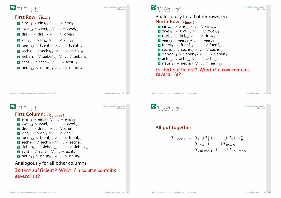
4 Knowledge Engineering (1)4.2 Sudoku
First Row: TRow 11 eins1,1 ∨ eins1,2 ∨ . . . ∨ eins1,9
2 zwei1,1 ∨ zwei1,2 ∨ . . . ∨ zwei1,93 drei1,1 ∨ drei1,2 ∨ . . . ∨ drei1,94 vier1,1 ∨ vier1,2 ∨ . . . ∨ vier1,9
5 fuenf1,1 ∨ fuenf1,2 ∨ . . . ∨ fuenf1,96 sechs1,1 ∨ sechs1,2 ∨ . . . ∨ sechs1,9
7 sieben1,1 ∨ sieben1,2 ∨ . . . ∨ sieben1,9
8 acht1,1 ∨ acht1,2 ∨ . . . ∨ acht1,9
9 neun1,1 ∨ neun1,2 ∨ . . . ∨ neun1,9
Prof. Dr. Jürgen Dix · Department of Informatics, TU Clausthal Artificial Intelligence, SS 09 301
4 Knowledge Engineering (1)4.2 Sudoku
Analogously for all other rows, eg.Ninth Row: TRow 9
1 eins9,1 ∨ eins9,2 ∨ . . . ∨ eins9,9
2 zwei9,1 ∨ zwei9,2 ∨ . . . ∨ zwei9,93 drei9,1 ∨ drei9,2 ∨ . . . ∨ drei9,94 vier9,1 ∨ vier9,2 ∨ . . . ∨ vier9,9
5 fuenf9,1 ∨ fuenf9,2 ∨ . . . ∨ fuenf9,96 sechs9,1 ∨ sechs9,2 ∨ . . . ∨ sechs9,9
7 sieben9,1 ∨ sieben9,2 ∨ . . . ∨ sieben9,9
8 acht9,1 ∨ acht9,2 ∨ . . . ∨ acht9,9
9 neun9,1 ∨ neun9,2 ∨ . . . ∨ neun9,9
Is that sufficient? What if a row containsseveral 1’s?
Prof. Dr. Jürgen Dix · Department of Informatics, TU Clausthal Artificial Intelligence, SS 09 302
4 Knowledge Engineering (1)4.2 Sudoku
First Column: TColumn 11 eins1,1 ∨ eins2,1 ∨ . . . ∨ eins9,1
2 zwei1,1 ∨ zwei2,1 ∨ . . . ∨ zwei9,13 drei1,1 ∨ drei2,1 ∨ . . . ∨ drei9,14 vier1,1 ∨ vier2,1 ∨ . . . ∨ vier9,1
5 fuenf1,1 ∨ fuenf2,1 ∨ . . . ∨ fuenf9,16 sechs1,1 ∨ sechs2,1 ∨ . . . ∨ sechs9,1
7 sieben1,1 ∨ sieben2,1 ∨ . . . ∨ sieben9,1
8 acht1,1 ∨ acht2,1 ∨ . . . ∨ acht9,1
9 neun1,1 ∨ neun2,1 ∨ . . . ∨ neun9,1
Analogously for all other columns.
Is that sufficient? What if a column containsseveral 1’s?
Prof. Dr. Jürgen Dix · Department of Informatics, TU Clausthal Artificial Intelligence, SS 09 303
4 Knowledge Engineering (1)4.2 Sudoku
All put together:
TSudoku = T1 ∪ T ′1 ∪ . . . ∪ T9 ∪ T ′9TRow 1 ∪ . . . ∪ TRow 9
TColumn 1 ∪ . . . ∪ TColumn 9
Prof. Dr. Jürgen Dix · Department of Informatics, TU Clausthal Artificial Intelligence, SS 09 304
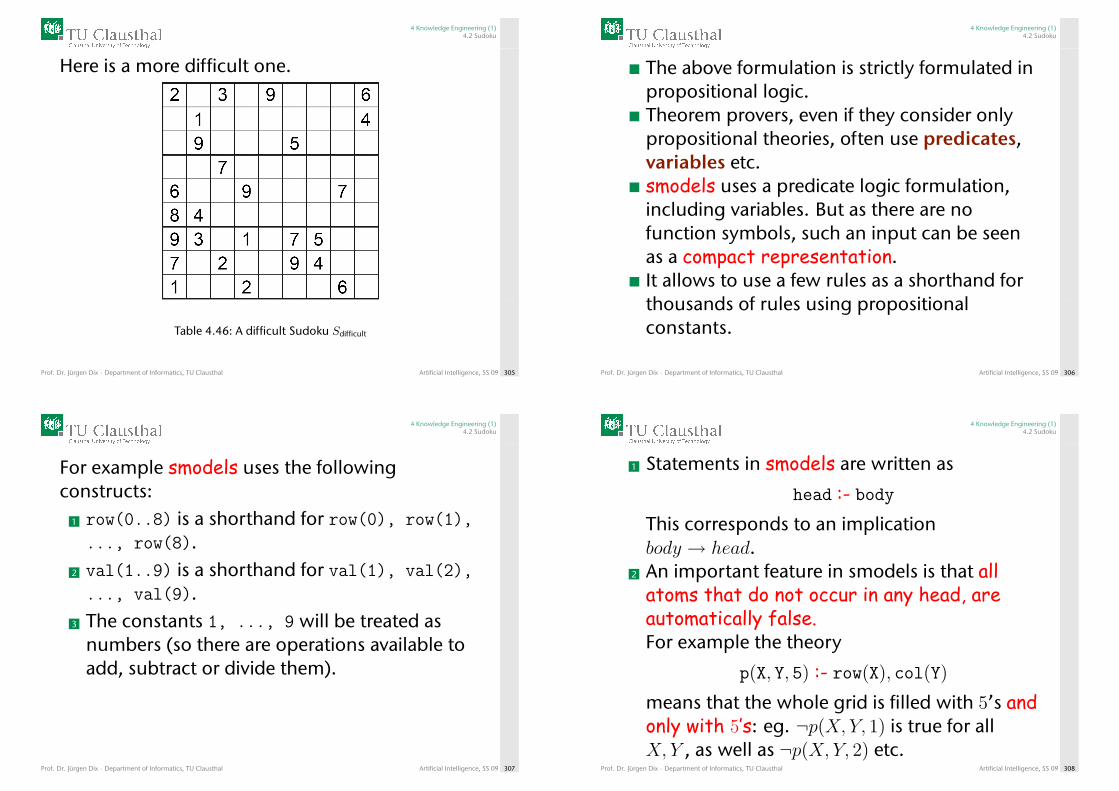
4 Knowledge Engineering (1)4.2 Sudoku
Here is a more difficult one.
Table 4.46: A difficult Sudoku Sdifficult
Prof. Dr. Jürgen Dix · Department of Informatics, TU Clausthal Artificial Intelligence, SS 09 305
4 Knowledge Engineering (1)4.2 Sudoku
The above formulation is strictly formulated inpropositional logic.Theorem provers, even if they consider onlypropositional theories, often use predicates,variables etc.smodels uses a predicate logic formulation,including variables. But as there are nofunction symbols, such an input can be seenas a compact representation.It allows to use a few rules as a shorthand forthousands of rules using propositionalconstants.
Prof. Dr. Jürgen Dix · Department of Informatics, TU Clausthal Artificial Intelligence, SS 09 306
4 Knowledge Engineering (1)4.2 Sudoku
For example smodels uses the followingconstructs:
1 row(0..8) is a shorthand for row(0), row(1),..., row(8).
2 val(1..9) is a shorthand for val(1), val(2),..., val(9).
3 The constants 1, ..., 9 will be treated asnumbers (so there are operations available toadd, subtract or divide them).
Prof. Dr. Jürgen Dix · Department of Informatics, TU Clausthal Artificial Intelligence, SS 09 307
4 Knowledge Engineering (1)4.2 Sudoku
1 Statements in smodels are written as
head :- bodyThis corresponds to an implicationbody → head.
2 An important feature in smodels is that allatoms that do not occur in any head, areautomatically false.For example the theory
p(X, Y, 5) :- row(X), col(Y)
means that the whole grid is filled with 5’s andonly with 5’s: eg. ¬p(X, Y, 1) is true for allX, Y , as well as ¬p(X, Y, 2) etc.
Prof. Dr. Jürgen Dix · Department of Informatics, TU Clausthal Artificial Intelligence, SS 09 308
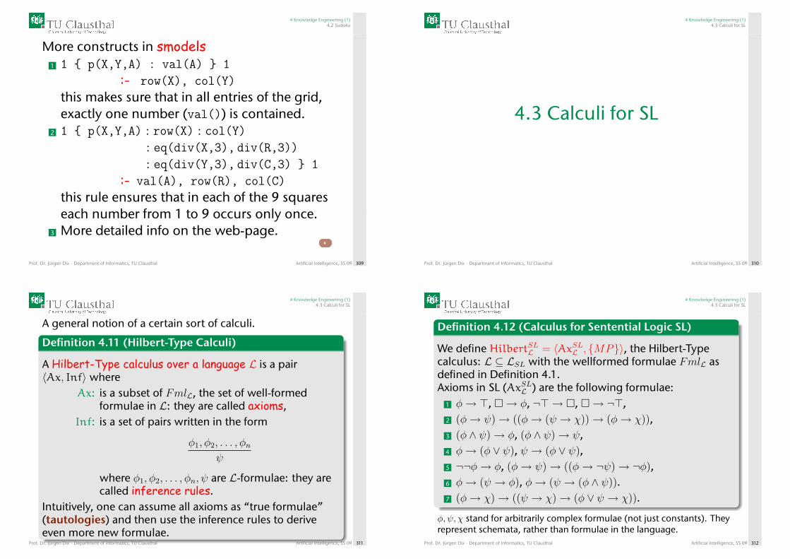
4 Knowledge Engineering (1)4.2 Sudoku
More constructs in smodels1 1 { p(X,Y,A) : val(A) } 1
:- row(X), col(Y)this makes sure that in all entries of the grid,exactly one number (val()) is contained.
2 1 { p(X,Y,A) : row(X) : col(Y): eq(div(X,3), div(R,3)): eq(div(Y,3), div(C,3) } 1
:- val(A), row(R), col(C)this rule ensures that in each of the 9 squareseach number from 1 to 9 occurs only once.
3 More detailed info on the web-page.
Prof. Dr. Jürgen Dix · Department of Informatics, TU Clausthal Artificial Intelligence, SS 09 309
4 Knowledge Engineering (1)4.3 Calculi for SL
4.3 Calculi for SL
Prof. Dr. Jürgen Dix · Department of Informatics, TU Clausthal Artificial Intelligence, SS 09 310
4 Knowledge Engineering (1)4.3 Calculi for SL
A general notion of a certain sort of calculi.
Definition 4.11 (Hilbert-Type Calculi)
A Hilbert-Type calculus over a language L is a pair〈Ax, Inf〉 where
Ax: is a subset of FmlL, the set of well-formedformulae in L: they are called axioms,
Inf: is a set of pairs written in the form
φ1, φ2, . . . , φnψ
where φ1, φ2, . . . , φn, ψ are L-formulae: they arecalled inference rules.
Intuitively, one can assume all axioms as “true formulae”(tautologies) and then use the inference rules to deriveeven more new formulae.
Prof. Dr. Jürgen Dix · Department of Informatics, TU Clausthal Artificial Intelligence, SS 09 311
4 Knowledge Engineering (1)4.3 Calculi for SL
Definition 4.12 (Calculus for Sentential Logic SL)
We define HilbertSLL = 〈AxSLL , {MP}〉, the Hilbert-Typecalculus: L ⊆ LSL with the wellformed formulae FmlL asdefined in Definition 4.1.Axioms in SL (AxSLL ) are the following formulae:
1 φ→ >, �→ φ, ¬> → �, �→ ¬>,2 (φ→ ψ)→ ((φ→ (ψ → χ))→ (φ→ χ)),3 (φ ∧ ψ)→ φ, (φ ∧ ψ)→ ψ,4 φ→ (φ ∨ ψ), ψ → (φ ∨ ψ),5 ¬¬φ→ φ, (φ→ ψ)→ ((φ→ ¬ψ)→ ¬φ),6 φ→ (ψ → φ), φ→ (ψ → (φ ∧ ψ)).7 (φ→ χ)→ ((ψ → χ)→ (φ ∨ ψ → χ)).
φ, ψ, χ stand for arbitrarily complex formulae (not just constants). Theyrepresent schemata, rather than formulae in the language.
Prof. Dr. Jürgen Dix · Department of Informatics, TU Clausthal Artificial Intelligence, SS 09 312
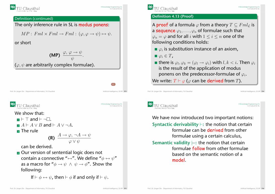
4 Knowledge Engineering (1)4.3 Calculi for SL
Definition (continued)
The only inference rule in SL is modus ponens:
MP : Fml × Fml→ Fml : (ϕ, ϕ→ ψ) 7→ ψ.
or short
(MP)ϕ, ϕ→ ψ
ψ.
(ϕ, ψ are arbitrarily complex formulae).
Prof. Dr. Jürgen Dix · Department of Informatics, TU Clausthal Artificial Intelligence, SS 09 313
4 Knowledge Engineering (1)4.3 Calculi for SL
Definition 4.13 (Proof)
A proof of a formula ϕ from a theory T ⊆ FmlL isa sequence ϕ1, . . . , ϕn of formulae such thatϕn = ϕ and for all i with 1 ≤ i ≤ n one of thefollowing conditions holds:
ϕi is substitution instance of an axiom,ϕi ∈ T ,there is ϕl, ϕk = (ϕl → ϕi) with l, k < i. Then ϕiis the result of the application of modusponens on the predecessor-formulae of ϕi.
We write: T ` ϕ (ϕ can be derived from T ).
Prof. Dr. Jürgen Dix · Department of Informatics, TU Clausthal Artificial Intelligence, SS 09 314
4 Knowledge Engineering (1)4.3 Calculi for SL
We show that:1 ` > and ` ¬�.2 A ` A ∨B and ` A ∨ ¬A.3 The rule
(R)A→ ϕ, ¬A→ ψ
ϕ ∨ ψcan be derived.
4 Our version of sentential logic does notcontain a connective “↔”. We define “φ↔ ψ”as a macro for “φ→ ψ ∧ ψ → φ”. Show thefollowing:
If ` φ↔ ψ, then ` φ if and only if ` ψ.
Prof. Dr. Jürgen Dix · Department of Informatics, TU Clausthal Artificial Intelligence, SS 09 315
4 Knowledge Engineering (1)4.3 Calculi for SL
We have now introduced two important notions:Syntactic derivability `: the notion that certain
formulae can be derived from otherformulae using a certain calculus,
Semantic validity |=: the notion that certainformulae follow from other formulaebased on the semantic notion of amodel.
Prof. Dr. Jürgen Dix · Department of Informatics, TU Clausthal Artificial Intelligence, SS 09 316
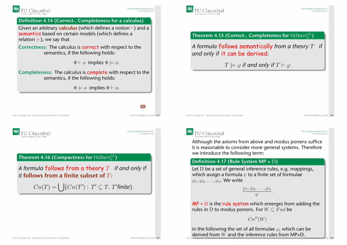
4 Knowledge Engineering (1)4.3 Calculi for SL
Definition 4.14 (Correct-, Completeness for a calculus)Given an arbitrary calculus (which defines a notion `) and asemantics based on certain models (which defines arelation |=), we say that
Correctness: The calculus is correct with respect to thesemantics, if the following holds:
Φ ` φ implies Φ |= φ.
Completeness: The calculus is complete with respect to thesemantics, if the following holds:
Φ |= φ implies Φ ` φ.
Prof. Dr. Jürgen Dix · Department of Informatics, TU Clausthal Artificial Intelligence, SS 09 317
4 Knowledge Engineering (1)4.3 Calculi for SL
Theorem 4.15 (Correct-, Completeness for HilbertSLL )
A formula follows semantically from a theory T ifand only if it can be derived:
T |= ϕ if and only if T ` ϕ
Prof. Dr. Jürgen Dix · Department of Informatics, TU Clausthal Artificial Intelligence, SS 09 318
4 Knowledge Engineering (1)4.3 Calculi for SL
Theorem 4.16 (Compactness for HilbertSLL )
A formula follows from a theory T if and only ifit follows from a finite subset of T :
Cn(T ) =⋃{Cn(T ′) : T ′ ⊆ T, T ′finite}.
Prof. Dr. Jürgen Dix · Department of Informatics, TU Clausthal Artificial Intelligence, SS 09 319
4 Knowledge Engineering (1)4.3 Calculi for SL
Although the axioms from above and modus ponens sufficeit is reasonable to consider more general systems. Thereforewe introduce the following term:
Definition 4.17 (Rule System MP + D)Let D be a set of general inference rules, e.g. mappings,which assign a formula ψ to a finite set of formulaeϕ1, ϕ2, . . . , ϕn. We write
ϕ1, ϕ2, . . . , ϕnψ
.
MP + D is the rule system which emerges from adding therules in D to modus ponens. For W ⊆ Fml be
CnD(W )
in the following the set of all formulae ϕ, which can bederived from W and the inference rules from MP+D.
Prof. Dr. Jürgen Dix · Department of Informatics, TU Clausthal Artificial Intelligence, SS 09 320
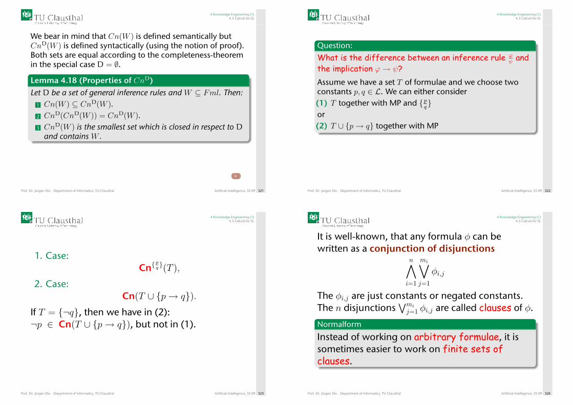
4 Knowledge Engineering (1)4.3 Calculi for SL
We bear in mind that Cn(W ) is defined semantically butCnD(W ) is defined syntactically (using the notion of proof).Both sets are equal according to the completeness-theoremin the special case D = ∅.
Lemma 4.18 (Properties of CnD)Let D be a set of general inference rules and W ⊆ Fml. Then:
1 Cn(W ) ⊆ CnD(W ).2 CnD(CnD(W )) = CnD(W ).3 CnD(W ) is the smallest set which is closed in respect to D
and contains W .
Prof. Dr. Jürgen Dix · Department of Informatics, TU Clausthal Artificial Intelligence, SS 09 321
4 Knowledge Engineering (1)4.3 Calculi for SL
Question:
What is the difference between an inference rule ϕψand
the implication ϕ→ ψ?Assume we have a set T of formulae and we choose twoconstants p, q ∈ L. We can either consider(1) T together with MP and {p
q}
or(2) T ∪ {p→ q} together with MP
Prof. Dr. Jürgen Dix · Department of Informatics, TU Clausthal Artificial Intelligence, SS 09 322
4 Knowledge Engineering (1)4.3 Calculi for SL
1. Case:Cn{
pq }(T ),
2. Case:Cn(T ∪ {p→ q}).
If T = {¬q}, then we have in (2):¬p ∈ Cn(T ∪ {p→ q}), but not in (1).
Prof. Dr. Jürgen Dix · Department of Informatics, TU Clausthal Artificial Intelligence, SS 09 323
4 Knowledge Engineering (1)4.3 Calculi for SL
It is well-known, that any formula φ can bewritten as a conjunction of disjunctions
n∧i=1
mi∨j=1
φi,j
The φi,j are just constants or negated constants.The n disjunctions
∨mi
j=1 φi,j are called clauses of φ.
Normalform
Instead of working on arbitrary formulae, it issometimes easier to work on finite sets ofclauses.
Prof. Dr. Jürgen Dix · Department of Informatics, TU Clausthal Artificial Intelligence, SS 09 324
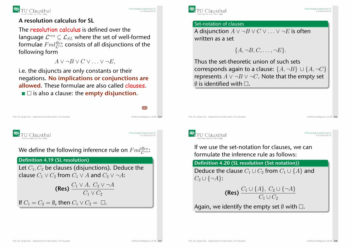
4 Knowledge Engineering (1)4.3 Calculi for SL
A resolution calculus for SL
The resolution calculus is defined over thelanguage Lres ⊆ LSL where the set of well-formedformulae FmlResLres consists of all disjunctions of thefollowing form
A ∨ ¬B ∨ C ∨ . . . ∨ ¬E,i.e. the disjuncts are only constants or theirnegations. No implications or conjunctions areallowed. These formulae are also called clauses.� is also a clause: the empty disjunction.
Prof. Dr. Jürgen Dix · Department of Informatics, TU Clausthal Artificial Intelligence, SS 09 325
4 Knowledge Engineering (1)4.3 Calculi for SL
Set-notation of clauses
A disjunction A ∨ ¬B ∨ C ∨ . . . ∨ ¬E is oftenwritten as a set
{A,¬B,C, . . . ,¬E}.
Thus the set-theoretic union of such setscorresponds again to a clause: {A,¬B} ∪ {A,¬C}represents A ∨ ¬B ∨ ¬C. Note that the empty set∅ is identified with �.
Prof. Dr. Jürgen Dix · Department of Informatics, TU Clausthal Artificial Intelligence, SS 09 326
4 Knowledge Engineering (1)4.3 Calculi for SL
We define the following inference rule on FmlResLres:
Definition 4.19 (SL resolution)
Let C1, C2 be clauses (disjunctions). Deduce theclause C1 ∨ C2 from C1 ∨ A and C2 ∨ ¬A:
(Res)C1 ∨ A, C2 ∨ ¬A
C1 ∨ C2
If C1 = C2 = ∅, then C1 ∨ C2 = �.
Prof. Dr. Jürgen Dix · Department of Informatics, TU Clausthal Artificial Intelligence, SS 09 327
4 Knowledge Engineering (1)4.3 Calculi for SL
If we use the set-notation for clauses, we canformulate the inference rule as follows:Definition 4.20 (SL resolution (Set notation))
Deduce the clause C1 ∪ C2 from C1 ∪ {A} andC2 ∪ {¬A}:
(Res)C1 ∪ {A}, C2 ∪ {¬A}
C1 ∪ C2
Again, we identify the empty set ∅ with �.
Prof. Dr. Jürgen Dix · Department of Informatics, TU Clausthal Artificial Intelligence, SS 09 328
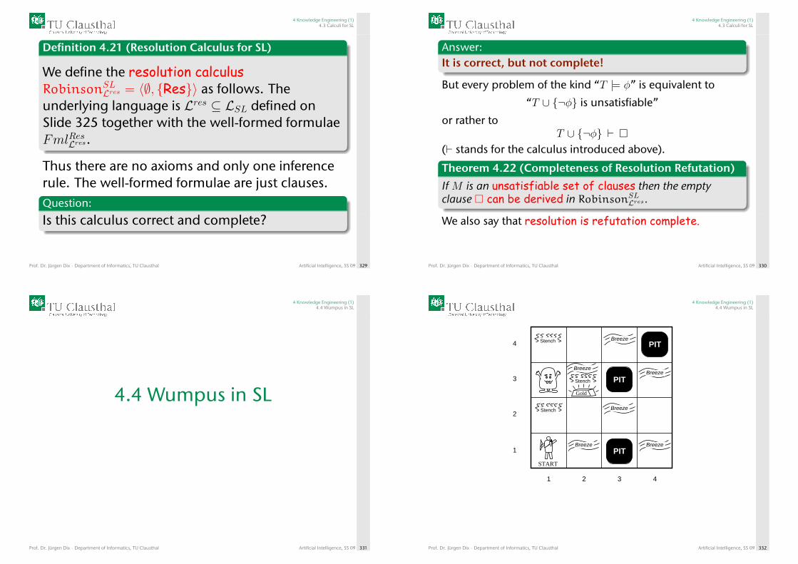
4 Knowledge Engineering (1)4.3 Calculi for SL
Definition 4.21 (Resolution Calculus for SL)
We define the resolution calculusRobinsonSL
Lres = 〈∅, {Res}〉 as follows. Theunderlying language is Lres ⊆ LSL defined onSlide 325 together with the well-formed formulaeFmlResLres.
Thus there are no axioms and only one inferencerule. The well-formed formulae are just clauses.Question:
Is this calculus correct and complete?
Prof. Dr. Jürgen Dix · Department of Informatics, TU Clausthal Artificial Intelligence, SS 09 329
4 Knowledge Engineering (1)4.3 Calculi for SL
Answer:It is correct, but not complete!
But every problem of the kind “T |= φ” is equivalent to
“T ∪ {¬φ} is unsatisfiable”
or rather toT ∪ {¬φ} ` �
(` stands for the calculus introduced above).
Theorem 4.22 (Completeness of Resolution Refutation)
If M is an unsatisfiable set of clauses then the emptyclause � can be derived in RobinsonSL
Lres.
We also say that resolution is refutation complete.
Prof. Dr. Jürgen Dix · Department of Informatics, TU Clausthal Artificial Intelligence, SS 09 330
4 Knowledge Engineering (1)4.4 Wumpus in SL
4.4 Wumpus in SL
Prof. Dr. Jürgen Dix · Department of Informatics, TU Clausthal Artificial Intelligence, SS 09 331
4 Knowledge Engineering (1)4.4 Wumpus in SL
Breeze Breeze
Breeze
BreezeBreeze
Stench
Stench
BreezePIT
PIT
PIT
1 2 3 4
1
2
3
4
START
Gold
Stench
Prof. Dr. Jürgen Dix · Department of Informatics, TU Clausthal Artificial Intelligence, SS 09 332
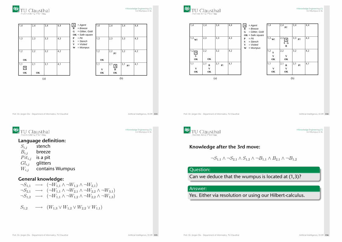
4 Knowledge Engineering (1)4.4 Wumpus in SL
ABG
PS
W
= Agent = Breeze = Glitter, Gold
= Pit = Stench
= Wumpus
OK = Safe square
V = Visited
A
OK
1,1 2,1 3,1 4,1
1,2 2,2 3,2 4,2
1,3 2,3 3,3 4,3
1,4 2,4 3,4 4,4
OKOKB
P?
P?A
OK OK
OK
1,1 2,1 3,1 4,1
1,2 2,2 3,2 4,2
1,3 2,3 3,3 4,3
1,4 2,4 3,4 4,4
V
(a) (b)
Prof. Dr. Jürgen Dix · Department of Informatics, TU Clausthal Artificial Intelligence, SS 09 333
4 Knowledge Engineering (1)4.4 Wumpus in SL
BB P!
A
OK OK
OK
1,1 2,1 3,1 4,1
1,2 2,2 3,2 4,2
1,3 2,3 3,3 4,3
1,4 2,4 3,4 4,4
V
OK
W!
VP!
A
OK OK
OK
1,1 2,1 3,1 4,1
1,2 2,2 3,2 4,2
1,3 2,3 3,3 4,3
1,4 2,4 3,4 4,4
V
S
OK
W!
V
V V
BS G
P?
P?
(b)(a)
S
ABG
PS
W
= Agent = Breeze = Glitter, Gold
= Pit = Stench
= Wumpus
OK = Safe square
V = Visited
Prof. Dr. Jürgen Dix · Department of Informatics, TU Clausthal Artificial Intelligence, SS 09 334
4 Knowledge Engineering (1)4.4 Wumpus in SL
Language definition:Si,j stenchBi,j breezePiti,j is a pitGli,j glittersWi,j contains Wumpus
General knowledge:¬S1,1 −→ (¬W1,1 ∧ ¬W1,2 ∧ ¬W2,1)¬S2,1 −→ (¬W1,1 ∧ ¬W2,1 ∧ ¬W2,2 ∧ ¬W3,1)¬S1,2 −→ (¬W1,1 ∧ ¬W1,2 ∧ ¬W2,2 ∧ ¬W1,3)
S1,2 −→ (W1,3 ∨W1,2 ∨W2,2 ∨W1,1)
Prof. Dr. Jürgen Dix · Department of Informatics, TU Clausthal Artificial Intelligence, SS 09 335
4 Knowledge Engineering (1)4.4 Wumpus in SL
Knowledge after the 3rd move:
¬S1,1 ∧ ¬S2,1 ∧ S1,2 ∧ ¬B1,1 ∧B2,1 ∧ ¬B1,2
Question:Can we deduce that the wumpus is located at (1,3)?
Answer:Yes. Either via resolution or using our Hilbert-calculus.
Prof. Dr. Jürgen Dix · Department of Informatics, TU Clausthal Artificial Intelligence, SS 09 336
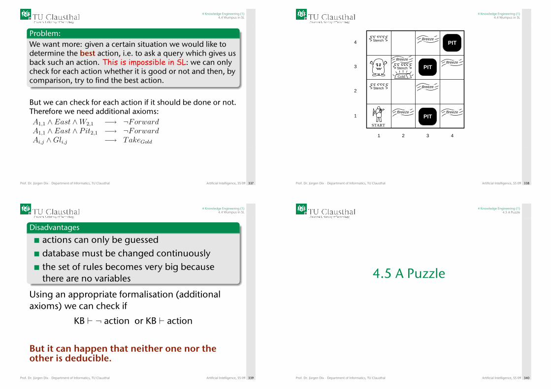
4 Knowledge Engineering (1)4.4 Wumpus in SL
Problem:We want more: given a certain situation we would like todetermine the best action, i.e. to ask a query which gives usback such an action. This is impossible in SL: we can onlycheck for each action whether it is good or not and then, bycomparison, try to find the best action.
But we can check for each action if it should be done or not.Therefore we need additional axioms:A1,1 ∧ East ∧W2,1 −→ ¬ForwardA1,1 ∧ East ∧ Pit2,1 −→ ¬ForwardAi,j ∧Gli,j −→ TakeGold
Prof. Dr. Jürgen Dix · Department of Informatics, TU Clausthal Artificial Intelligence, SS 09 337
4 Knowledge Engineering (1)4.4 Wumpus in SL
Breeze Breeze
Breeze
BreezeBreeze
Stench
Stench
BreezePIT
PIT
PIT
1 2 3 4
1
2
3
4
START
Gold
Stench
Prof. Dr. Jürgen Dix · Department of Informatics, TU Clausthal Artificial Intelligence, SS 09 338
4 Knowledge Engineering (1)4.4 Wumpus in SL
Disadvantages
actions can only be guesseddatabase must be changed continuouslythe set of rules becomes very big becausethere are no variables
Using an appropriate formalisation (additionalaxioms) we can check if
KB ` ¬ action or KB ` action
But it can happen that neither one nor theother is deducible.
Prof. Dr. Jürgen Dix · Department of Informatics, TU Clausthal Artificial Intelligence, SS 09 339
4 Knowledge Engineering (1)4.5 A Puzzle
4.5 A Puzzle
Prof. Dr. Jürgen Dix · Department of Informatics, TU Clausthal Artificial Intelligence, SS 09 340
4 Knowledge Engineering (1)4.5 A Puzzle
We now want to formalize a ”Logelei“ and solve itwith a theorem prover.
”Logelei“ from ”Die Zeit“ (1)
Alfred ist als neuer Korrespondent in Wongowongo. Er sollüber die Präsidentschaftswahlen berichten, weiß aber nochnichts über die beiden Kandidaten, weswegen er sich unterdie Leute begibt, um Infos zu sammeln. Er befragt eineGruppe von Passanten, von denen drei Anhänger derEntweder-oder-Partei sind und drei Anhänger derKonsequenten.
Prof. Dr. Jürgen Dix · Department of Informatics, TU Clausthal Artificial Intelligence, SS 09 341
4 Knowledge Engineering (1)4.5 A Puzzle
”Logelei“ from ”Die Zeit“ (2)
Auf seinem Notizzettel notiert er stichwortartig dieAntworten.A: »Nachname Songo: Stadt Rongo«,B: »Entweder-oder-Partei: älter«,C: »Vorname Dongo: bei Umfrage hinten«,A: »Konsequenten: Vorname Mongo«,B: »Stamm Bongo: Nachname Gongo«,C: »Vorname Dongo: jünger«,D: »Stamm Bongo: bei Umfrage vorn«,E: »Vorname Mongo: bei Umfrage hinten«,F: »Konsequenten: Stamm Nongo«,D: »Stadt Longo: jünger«,E: »Stamm Nongo: jünger«.F: »Konsequenten: Nachname Gongo«.
Prof. Dr. Jürgen Dix · Department of Informatics, TU Clausthal Artificial Intelligence, SS 09 342
4 Knowledge Engineering (1)4.5 A Puzzle
”Logelei“ from ”Die Zeit“ (3)
Jetzt grübelt Alfred. Er weiß, dass die Anhängerder Entweder-oder-Partei (A, B und C) immer einerichtige und eine falsche Aussage machen,während die Anhänger der Konsequenten (D, Eund F) entweder nur wahre Aussagen oder nurfalsche Aussagen machen.Welche Informationen hat Alfred über die beidenKandidaten?
(By Zweistein)
Prof. Dr. Jürgen Dix · Department of Informatics, TU Clausthal Artificial Intelligence, SS 09 343
4 Knowledge Engineering (1)4.5 A Puzzle
Towards a solution
Selection of the language (Propositional Logic,Predicate Logic,...).Analysis and formalization of the problem.Transformation to the input format of a prover.Output of a solution, i.e. a model.
Prof. Dr. Jürgen Dix · Department of Informatics, TU Clausthal Artificial Intelligence, SS 09 344
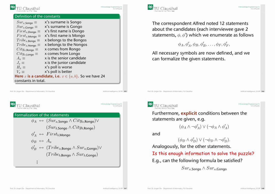
4 Knowledge Engineering (1)4.5 A Puzzle
Definition of the constantsSurx,Songo ≡ x’s surname is SongoSurx,Gongo ≡ x’s surname is GongoFirstx,Dongo ≡ x’s first name is DongoFirstx,Mongo ≡ x’s first name is MongoTribex,Bongo ≡ x belongs to the BongosTribex,Nongo ≡ x belongs to the NongosCityx,Rongo ≡ x comes from RongoCityx,Longo ≡ x comes from LongoAx ≡ x is the senior candidateJx ≡ x is the junior candidateHx ≡ x’s poll is worseVx ≡ x’s poll is better
Here x is a candidate, i.e. x ∈ {a, b}. So we have 24constants in total.
Prof. Dr. Jürgen Dix · Department of Informatics, TU Clausthal Artificial Intelligence, SS 09 345
4 Knowledge Engineering (1)4.5 A Puzzle
The correspondent Alfred noted 12 statementsabout the candidates (each interviewee gave 2statements, φ, φ′) which we enumerate as follows
φA, φ′A, φB, φ
′B, . . . , φF , φ
′F ,
All necessary symbols are now defined, and wecan formalize the given statements.
Prof. Dr. Jürgen Dix · Department of Informatics, TU Clausthal Artificial Intelligence, SS 09 346
4 Knowledge Engineering (1)4.5 A Puzzle
Formalization of the statementsφA ↔ (Sura,Songo ∧ Citya,Rongo)∨
(Surb,Songo ∧ Cityb,Rongo)
φ′A ↔ Firstb,Mongo
φB ↔ Aa
φ′B ↔ (Tribea,Bongo ∧ Sura,Gongo)∨(Tribeb,Bongo ∧ Surb,Gongo)
...
Prof. Dr. Jürgen Dix · Department of Informatics, TU Clausthal Artificial Intelligence, SS 09 347
4 Knowledge Engineering (1)4.5 A Puzzle
Furthermore, explicit conditions between thestatements are given, e.g.
(φA ∧ ¬φ′A) ∨ (¬φA ∧ φ′A)
and(φD ∧ φ′D) ∨ (¬φD ∧ ¬φ′D).
Analogously, for the other statements.
Is this enough information to solve the puzzle?E.g., can the following formula be satisfied?
Sura,Songo ∧ Sura,Gongo
Prof. Dr. Jürgen Dix · Department of Informatics, TU Clausthal Artificial Intelligence, SS 09 348
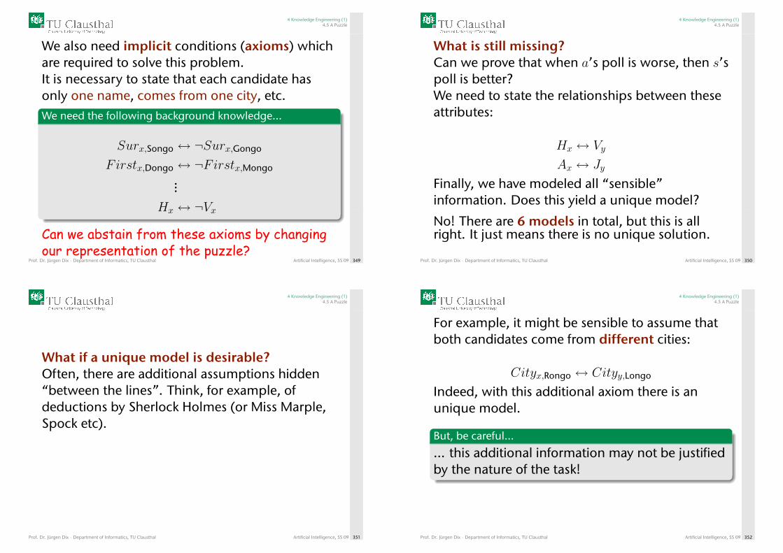
4 Knowledge Engineering (1)4.5 A Puzzle
We also need implicit conditions (axioms) whichare required to solve this problem.It is necessary to state that each candidate hasonly one name, comes from one city, etc.We need the following background knowledge...
Surx,Songo ↔ ¬Surx,Gongo
Firstx,Dongo ↔ ¬Firstx,Mongo...
Hx ↔ ¬Vx
Can we abstain from these axioms by changingour representation of the puzzle?
Prof. Dr. Jürgen Dix · Department of Informatics, TU Clausthal Artificial Intelligence, SS 09 349
4 Knowledge Engineering (1)4.5 A Puzzle
What is still missing?Can we prove that when a’s poll is worse, then s’spoll is better?We need to state the relationships between theseattributes:
Hx ↔ Vy
Ax ↔ Jy
Finally, we have modeled all “sensible”information. Does this yield a unique model?
No! There are 6 models in total, but this is allright. It just means there is no unique solution.
Prof. Dr. Jürgen Dix · Department of Informatics, TU Clausthal Artificial Intelligence, SS 09 350
4 Knowledge Engineering (1)4.5 A Puzzle
What if a unique model is desirable?Often, there are additional assumptions hidden“between the lines”. Think, for example, ofdeductions by Sherlock Holmes (or Miss Marple,Spock etc).
Prof. Dr. Jürgen Dix · Department of Informatics, TU Clausthal Artificial Intelligence, SS 09 351
4 Knowledge Engineering (1)4.5 A Puzzle
For example, it might be sensible to assume thatboth candidates come from different cities:
Cityx,Rongo ↔ Cityy,Longo
Indeed, with this additional axiom there is anunique model.
But, be careful...
... this additional information may not be justifiedby the nature of the task!
Prof. Dr. Jürgen Dix · Department of Informatics, TU Clausthal Artificial Intelligence, SS 09 352
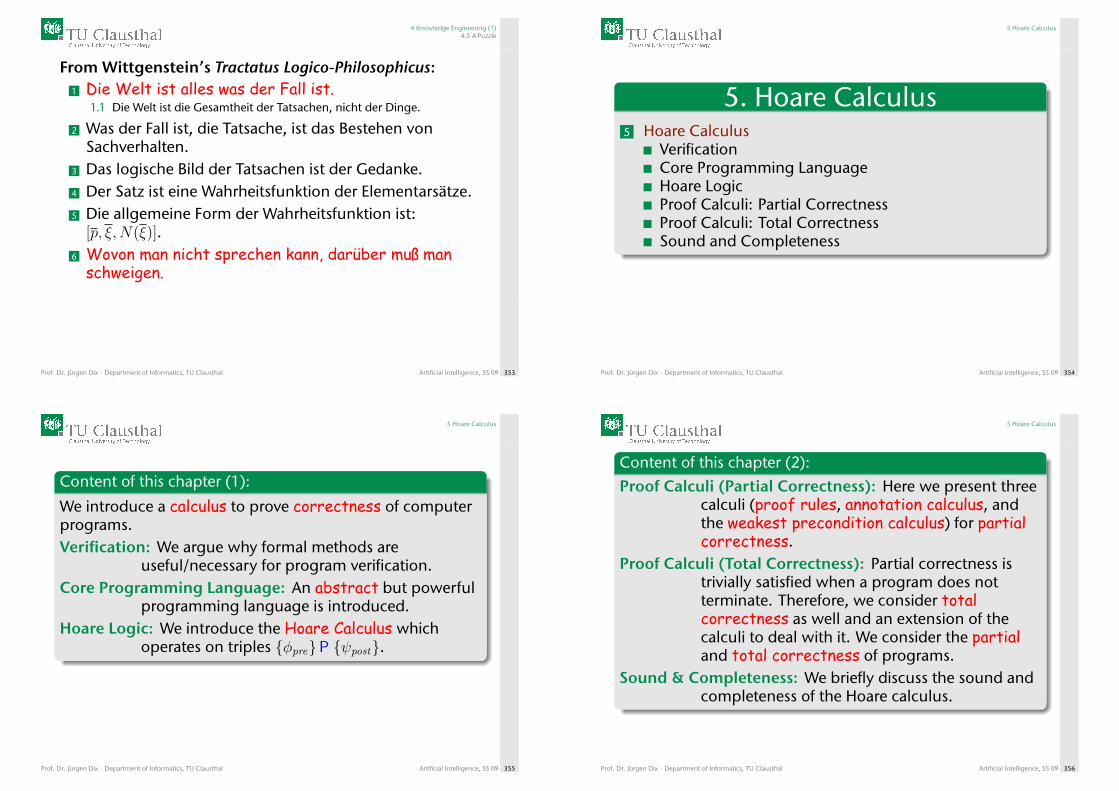
4 Knowledge Engineering (1)4.5 A Puzzle
From Wittgenstein’s Tractatus Logico-Philosophicus:1 Die Welt ist alles was der Fall ist.
1.1 Die Welt ist die Gesamtheit der Tatsachen, nicht der Dinge.
2 Was der Fall ist, die Tatsache, ist das Bestehen vonSachverhalten.
3 Das logische Bild der Tatsachen ist der Gedanke.4 Der Satz ist eine Wahrheitsfunktion der Elementarsätze.5 Die allgemeine Form der Wahrheitsfunktion ist:
[p, ξ,N(ξ)].6 Wovon man nicht sprechen kann, darüber muß manschweigen.
Prof. Dr. Jürgen Dix · Department of Informatics, TU Clausthal Artificial Intelligence, SS 09 353
5 Hoare Calculus
5. Hoare Calculus5 Hoare Calculus
VerificationCore Programming LanguageHoare LogicProof Calculi: Partial CorrectnessProof Calculi: Total CorrectnessSound and Completeness
Prof. Dr. Jürgen Dix · Department of Informatics, TU Clausthal Artificial Intelligence, SS 09 354
5 Hoare Calculus
Content of this chapter (1):
We introduce a calculus to prove correctness of computerprograms.Verification: We argue why formal methods are
useful/necessary for program verification.Core Programming Language: An abstract but powerful
programming language is introduced.Hoare Logic: We introduce the Hoare Calculus which
operates on triples {φpre}P {ψpost}.
Prof. Dr. Jürgen Dix · Department of Informatics, TU Clausthal Artificial Intelligence, SS 09 355
5 Hoare Calculus
Content of this chapter (2):
Proof Calculi (Partial Correctness): Here we present threecalculi (proof rules, annotation calculus, andthe weakest precondition calculus) for partialcorrectness.
Proof Calculi (Total Correctness): Partial correctness istrivially satisfied when a program does notterminate. Therefore, we consider totalcorrectness as well and an extension of thecalculi to deal with it. We consider the partialand total correctness of programs.
Sound & Completeness: We briefly discuss the sound andcompleteness of the Hoare calculus.
Prof. Dr. Jürgen Dix · Department of Informatics, TU Clausthal Artificial Intelligence, SS 09 356
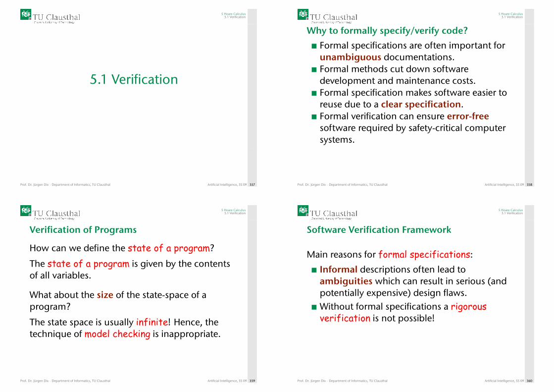
5 Hoare Calculus5.1 Verification
5.1 Verification
Prof. Dr. Jürgen Dix · Department of Informatics, TU Clausthal Artificial Intelligence, SS 09 357
5 Hoare Calculus5.1 Verification
Why to formally specify/verify code?
Formal specifications are often important forunambiguous documentations.Formal methods cut down softwaredevelopment and maintenance costs.Formal specification makes software easier toreuse due to a clear specification.Formal verification can ensure error-freesoftware required by safety-critical computersystems.
Prof. Dr. Jürgen Dix · Department of Informatics, TU Clausthal Artificial Intelligence, SS 09 358
5 Hoare Calculus5.1 Verification
Verification of Programs
How can we define the state of a program?
The state of a program is given by the contentsof all variables.
What about the size of the state-space of aprogram?
The state space is usually infinite! Hence, thetechnique of model checking is inappropriate.
Prof. Dr. Jürgen Dix · Department of Informatics, TU Clausthal Artificial Intelligence, SS 09 359
5 Hoare Calculus5.1 Verification
Software Verification Framework
Main reasons for formal specifications:
Informal descriptions often lead toambiguities which can result in serious (andpotentially expensive) design flaws.Without formal specifications a rigorousverification is not possible!
Prof. Dr. Jürgen Dix · Department of Informatics, TU Clausthal Artificial Intelligence, SS 09 360
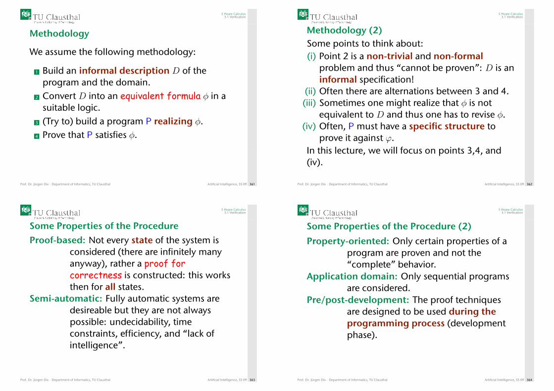
5 Hoare Calculus5.1 Verification
Methodology
We assume the following methodology:
1 Build an informal description D of theprogram and the domain.
2 Convert D into an equivalent formula φ in asuitable logic.
3 (Try to) build a program P realizing φ.4 Prove that P satisfies φ.
Prof. Dr. Jürgen Dix · Department of Informatics, TU Clausthal Artificial Intelligence, SS 09 361
5 Hoare Calculus5.1 Verification
Methodology (2)Some points to think about:(i) Point 2 is a non-trivial and non-formal
problem and thus “cannot be proven”: D is aninformal specification!
(ii) Often there are alternations between 3 and 4.(iii) Sometimes one might realize that φ is not
equivalent to D and thus one has to revise φ.(iv) Often, P must have a specific structure to
prove it against ϕ.In this lecture, we will focus on points 3,4, and(iv).
Prof. Dr. Jürgen Dix · Department of Informatics, TU Clausthal Artificial Intelligence, SS 09 362
5 Hoare Calculus5.1 Verification
Some Properties of the ProcedureProof-based: Not every state of the system is
considered (there are infinitely manyanyway), rather a proof forcorrectness is constructed: this worksthen for all states.
Semi-automatic: Fully automatic systems aredesireable but they are not alwayspossible: undecidability, timeconstraints, efficiency, and “lack ofintelligence”.
Prof. Dr. Jürgen Dix · Department of Informatics, TU Clausthal Artificial Intelligence, SS 09 363
5 Hoare Calculus5.1 Verification
Some Properties of the Procedure (2)
Property-oriented: Only certain properties of aprogram are proven and not the“complete” behavior.
Application domain: Only sequential programsare considered.
Pre/post-development: The proof techniquesare designed to be used during theprogramming process (developmentphase).
Prof. Dr. Jürgen Dix · Department of Informatics, TU Clausthal Artificial Intelligence, SS 09 364
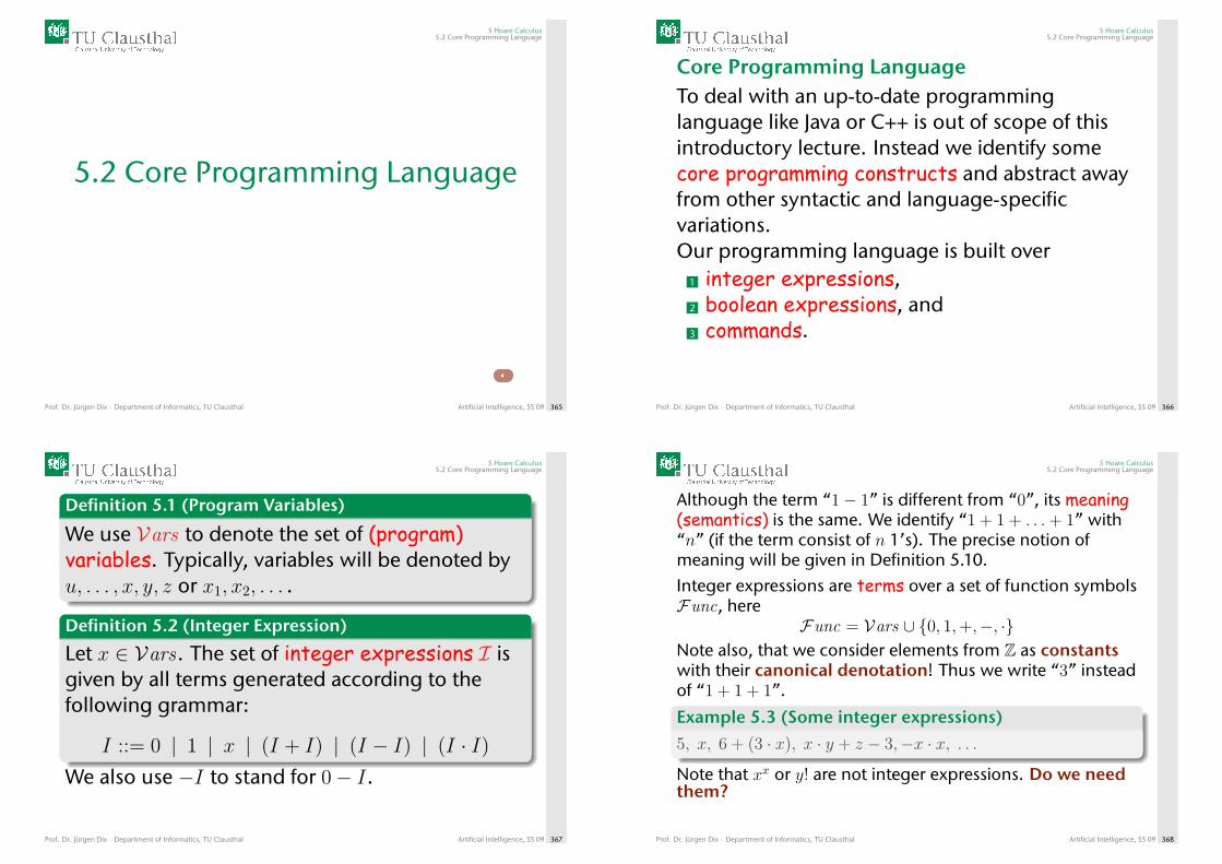
5 Hoare Calculus5.2 Core Programming Language
5.2 Core Programming Language
Prof. Dr. Jürgen Dix · Department of Informatics, TU Clausthal Artificial Intelligence, SS 09 365
5 Hoare Calculus5.2 Core Programming Language
Core Programming LanguageTo deal with an up-to-date programminglanguage like Java or C++ is out of scope of thisintroductory lecture. Instead we identify somecore programming constructs and abstract awayfrom other syntactic and language-specificvariations.Our programming language is built over
1 integer expressions,2 boolean expressions, and3 commands.
Prof. Dr. Jürgen Dix · Department of Informatics, TU Clausthal Artificial Intelligence, SS 09 366
5 Hoare Calculus5.2 Core Programming Language
Definition 5.1 (Program Variables)
We use Vars to denote the set of (program)variables. Typically, variables will be denoted byu, . . . , x, y, z or x1, x2, . . . .
Definition 5.2 (Integer Expression)
Let x ∈ Vars. The set of integer expressions I isgiven by all terms generated according to thefollowing grammar:
I ::= 0 | 1 | x | (I + I) | (I − I) | (I · I)
We also use −I to stand for 0− I.
Prof. Dr. Jürgen Dix · Department of Informatics, TU Clausthal Artificial Intelligence, SS 09 367
5 Hoare Calculus5.2 Core Programming Language
Although the term “1− 1” is different from “0”, its meaning(semantics) is the same. We identify “1 + 1 + . . .+ 1” with“n” (if the term consist of n 1’s). The precise notion ofmeaning will be given in Definition 5.10.Integer expressions are terms over a set of function symbolsFunc, here
Func = Vars ∪ {0, 1,+,−, ·}Note also, that we consider elements from Z as constantswith their canonical denotation! Thus we write “3” insteadof “1 + 1 + 1”.
Example 5.3 (Some integer expressions)
5, x, 6 + (3 · x), x · y + z − 3,−x · x, . . .
Note that xx or y! are not integer expressions. Do we needthem?
Prof. Dr. Jürgen Dix · Department of Informatics, TU Clausthal Artificial Intelligence, SS 09 368
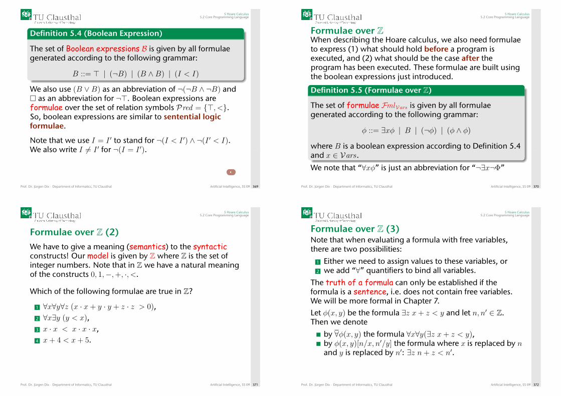
5 Hoare Calculus5.2 Core Programming Language
Definition 5.4 (Boolean Expression)
The set of Boolean expressions B is given by all formulaegenerated according to the following grammar:
B ::= > | (¬B) | (B ∧B) | (I < I)
We also use (B ∨B) as an abbreviation of ¬(¬B ∧ ¬B) and� as an abbreviation for ¬>. Boolean expressions areformulae over the set of relation symbols Pred = {>, <}.So, boolean expressions are similar to sentential logicformulae.
Note that we use I = I ′ to stand for ¬(I < I ′) ∧ ¬(I ′ < I).We also write I 6= I ′ for ¬(I = I ′).
Prof. Dr. Jürgen Dix · Department of Informatics, TU Clausthal Artificial Intelligence, SS 09 369
5 Hoare Calculus5.2 Core Programming Language
Formulae over ZWhen describing the Hoare calculus, we also need formulaeto express (1) what should hold before a program isexecuted, and (2) what should be the case after theprogram has been executed. These formulae are built usingthe boolean expressions just introduced.
Definition 5.5 (Formulae over Z)
The set of formulae FmlVars is given by all formulaegenerated according to the following grammar:
φ ::= ∃xφ | B | (¬φ) | (φ ∧ φ)
where B is a boolean expression according to Definition 5.4and x ∈ Vars.
We note that “∀xφ” is just an abbreviation for “¬∃x¬Φ”
Prof. Dr. Jürgen Dix · Department of Informatics, TU Clausthal Artificial Intelligence, SS 09 370
5 Hoare Calculus5.2 Core Programming Language
Formulae over Z (2)We have to give a meaning (semantics) to the syntacticconstructs! Our model is given by Z where Z is the set ofinteger numbers. Note that in Z we have a natural meaningof the constructs 0, 1,−,+, ·, <.
Which of the following formulae are true in Z?
1 ∀x∀y∀z (x · x+ y · y + z · z > 0),2 ∀x∃y (y < x),3 x · x < x · x · x,4 x+ 4 < x+ 5.
Prof. Dr. Jürgen Dix · Department of Informatics, TU Clausthal Artificial Intelligence, SS 09 371
5 Hoare Calculus5.2 Core Programming Language
Formulae over Z (3)Note that when evaluating a formula with free variables,there are two possibilities:
1 Either we need to assign values to these variables, or2 we add “∀” quantifiers to bind all variables.
The truth of a formula can only be established if theformula is a sentence, i.e. does not contain free variables.We will be more formal in Chapter 7.Let φ(x, y) be the formula ∃z x+ z < y and let n, n′ ∈ Z.Then we denote
by ∀φ(x, y) the formula ∀x∀y(∃z x+ z < y),by φ(x, y)[n/x, n′/y] the formula where x is replaced by nand y is replaced by n′: ∃z n+ z < n′.
Prof. Dr. Jürgen Dix · Department of Informatics, TU Clausthal Artificial Intelligence, SS 09 372
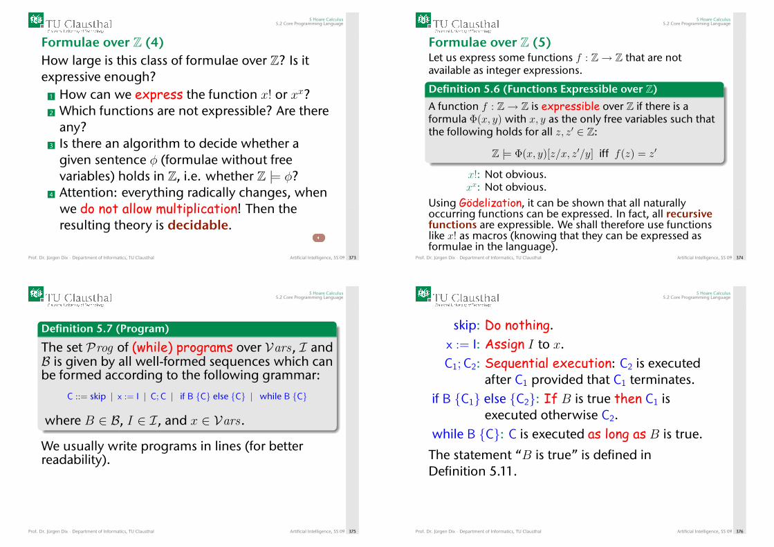
5 Hoare Calculus5.2 Core Programming Language
Formulae over Z (4)How large is this class of formulae over Z? Is itexpressive enough?
1 How can we express the function x! or xx?2 Which functions are not expressible? Are there
any?3 Is there an algorithm to decide whether a
given sentence φ (formulae without freevariables) holds in Z, i.e. whether Z |= φ?
4 Attention: everything radically changes, whenwe do not allow multiplication! Then theresulting theory is decidable.
Prof. Dr. Jürgen Dix · Department of Informatics, TU Clausthal Artificial Intelligence, SS 09 373
5 Hoare Calculus5.2 Core Programming Language
Formulae over Z (5)Let us express some functions f : Z→ Z that are notavailable as integer expressions.
Definition 5.6 (Functions Expressible over Z)
A function f : Z→ Z is expressible over Z if there is aformula Φ(x, y) with x, y as the only free variables such thatthe following holds for all z, z′ ∈ Z:
Z |= Φ(x, y)[z/x, z′/y] iff f(z) = z′
x!: Not obvious.xx: Not obvious.
Using Gödelization, it can be shown that all naturallyoccurring functions can be expressed. In fact, all recursivefunctions are expressible. We shall therefore use functionslike x! as macros (knowing that they can be expressed asformulae in the language).
Prof. Dr. Jürgen Dix · Department of Informatics, TU Clausthal Artificial Intelligence, SS 09 374
5 Hoare Calculus5.2 Core Programming Language
Definition 5.7 (Program)
The set Prog of (while) programs over Vars, I andB is given by all well-formed sequences which canbe formed according to the following grammar:
C ::= skip | x := I | C; C | if B {C} else {C} | while B {C}
where B ∈ B, I ∈ I, and x ∈ Vars.
We usually write programs in lines (for betterreadability).
Prof. Dr. Jürgen Dix · Department of Informatics, TU Clausthal Artificial Intelligence, SS 09 375
5 Hoare Calculus5.2 Core Programming Language
skip: Do nothing.x := I: Assign I to x.C1; C2: Sequential execution: C2 is executed
after C1 provided that C1 terminates.if B {C1} else {C2}: If B is true then C1 is
executed otherwise C2.while B {C}: C is executed as long as B is true.
The statement “B is true” is defined inDefinition 5.11.
Prof. Dr. Jürgen Dix · Department of Informatics, TU Clausthal Artificial Intelligence, SS 09 376
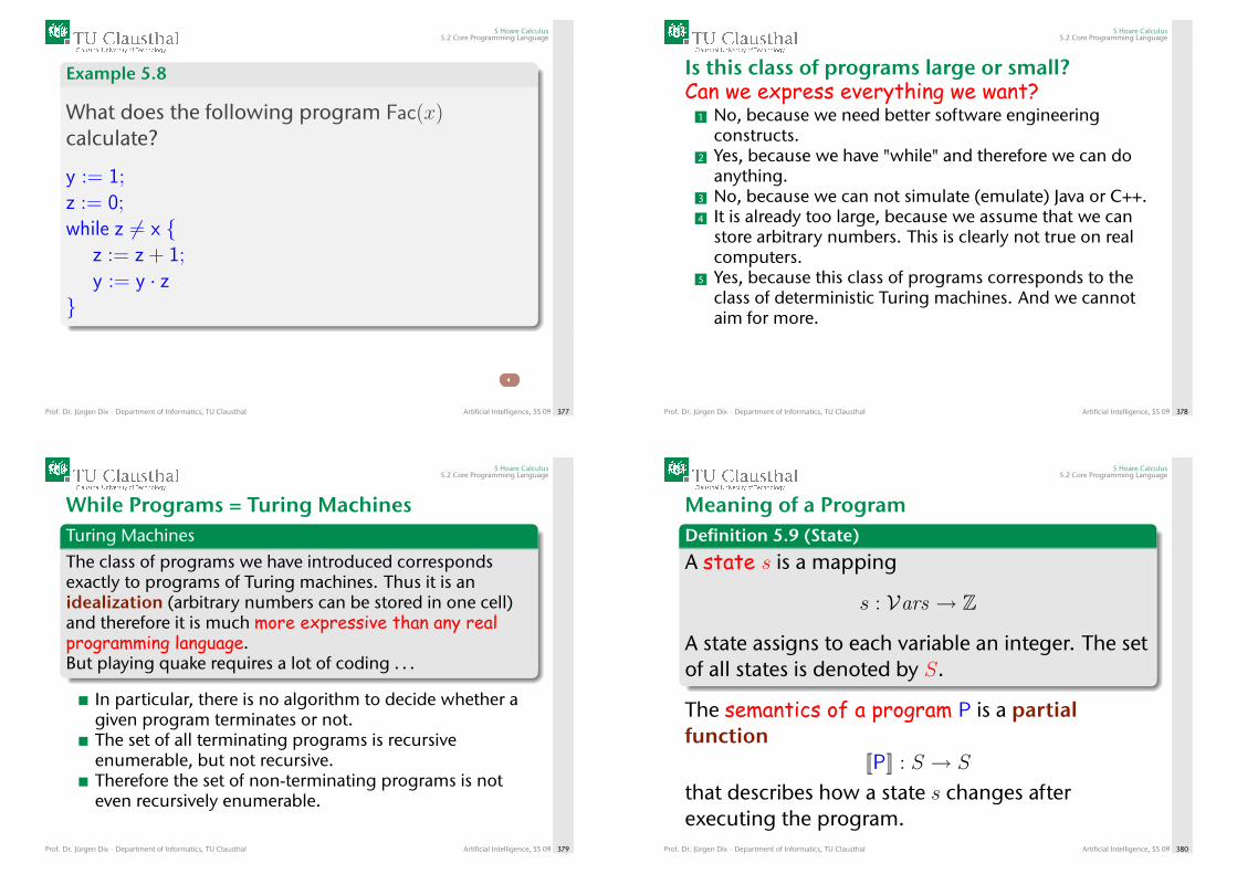
5 Hoare Calculus5.2 Core Programming Language
Example 5.8
What does the following program Fac(x)calculate?
y := 1;z := 0;while z 6= x {
z := z + 1;y := y · z
}
Prof. Dr. Jürgen Dix · Department of Informatics, TU Clausthal Artificial Intelligence, SS 09 377
5 Hoare Calculus5.2 Core Programming Language
Is this class of programs large or small?Can we express everything we want?
1 No, because we need better software engineeringconstructs.
2 Yes, because we have "while" and therefore we can doanything.
3 No, because we can not simulate (emulate) Java or C++.4 It is already too large, because we assume that we can
store arbitrary numbers. This is clearly not true on realcomputers.
5 Yes, because this class of programs corresponds to theclass of deterministic Turing machines. And we cannotaim for more.
Prof. Dr. Jürgen Dix · Department of Informatics, TU Clausthal Artificial Intelligence, SS 09 378
5 Hoare Calculus5.2 Core Programming Language
While Programs = Turing MachinesTuring Machines
The class of programs we have introduced correspondsexactly to programs of Turing machines. Thus it is anidealization (arbitrary numbers can be stored in one cell)and therefore it is much more expressive than any realprogramming language.But playing quake requires a lot of coding . . .
In particular, there is no algorithm to decide whether agiven program terminates or not.The set of all terminating programs is recursiveenumerable, but not recursive.Therefore the set of non-terminating programs is noteven recursively enumerable.
Prof. Dr. Jürgen Dix · Department of Informatics, TU Clausthal Artificial Intelligence, SS 09 379
5 Hoare Calculus5.2 Core Programming Language
Meaning of a ProgramDefinition 5.9 (State)
A state s is a mapping
s : Vars → Z
A state assigns to each variable an integer. The setof all states is denoted by S.
The semantics of a program P is a partialfunction
[[P]] : S → S
that describes how a state s changes afterexecuting the program.
Prof. Dr. Jürgen Dix · Department of Informatics, TU Clausthal Artificial Intelligence, SS 09 380
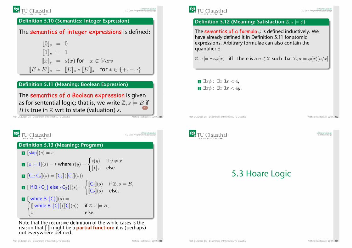
5 Hoare Calculus5.2 Core Programming Language
Definition 5.10 (Semantics: Integer Expression)
The semantics of integer expressions is defined:
[[0]]s = 0
[[1]]s = 1
[[x]]s = s(x) for x ∈ Vars
[[E ∗ E ′]]s = [[E]]s ∗ [[E ′]]s for ∗ ∈ {+,−, ·}
Definition 5.11 (Meaning: Boolean Expression)
The semantics of a Boolean expression is givenas for sentential logic; that is, we write Z, s |= B ifB is true in Z wrt to state (valuation) s.
Prof. Dr. Jürgen Dix · Department of Informatics, TU Clausthal Artificial Intelligence, SS 09 381
5 Hoare Calculus5.2 Core Programming Language
Definition 5.12 (Meaning: Satisfaction Z, s |= φ)
The semantics of a formula φ is defined inductively. Wehave already defined it in Definition 5.11 for atomicexpressions. Arbitrary formulae can also contain thequantifier ∃.
Z, s |= ∃xφ(x) iff there is a n ∈ Z such that Z, s |= φ(x)[n/x]
1 ∃xφ : ∃x 3x < 4,2 ∃xφ : ∃x 3x < 4y.
Prof. Dr. Jürgen Dix · Department of Informatics, TU Clausthal Artificial Intelligence, SS 09 382
5 Hoare Calculus5.2 Core Programming Language
Definition 5.13 (Meaning: Program)
1 [[skip]](s) = s
2 [[x := I]](s) = t where t(y) =
{s(y) if y 6= x
[[I]]s else.
3 [[C1; C2]](s) = [[C2]]([[C1]](s))
4 [[ if B {C1} else {C2}]](s) =
{[[C1]](s) if Z, s |= B,
[[C2]](s) else.
5 [[ while B {C}]](s) ={[[ while B {C}]]([[C]](s)) if Z, s |= B,
s else.
Note that the recursive definition of the while cases is thereason that [[·]] might be a partial function: it is (perhaps)not everywhere defined.
Prof. Dr. Jürgen Dix · Department of Informatics, TU Clausthal Artificial Intelligence, SS 09 383
5 Hoare Calculus5.3 Hoare Logic
5.3 Hoare Logic
Prof. Dr. Jürgen Dix · Department of Informatics, TU Clausthal Artificial Intelligence, SS 09 384
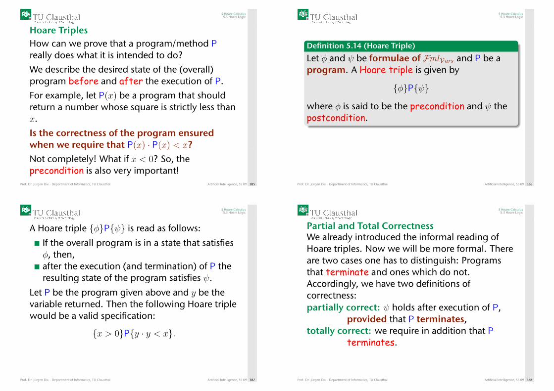
5 Hoare Calculus5.3 Hoare Logic
Hoare TriplesHow can we prove that a program/method Preally does what it is intended to do?
We describe the desired state of the (overall)program before and after the execution of P.
For example, let P(x) be a program that shouldreturn a number whose square is strictly less thanx.
Is the correctness of the program ensuredwhen we require that P(x) · P(x) < x?
Not completely! What if x < 0? So, theprecondition is also very important!
Prof. Dr. Jürgen Dix · Department of Informatics, TU Clausthal Artificial Intelligence, SS 09 385
5 Hoare Calculus5.3 Hoare Logic
Definition 5.14 (Hoare Triple)
Let φ and ψ be formulae of FmlVars and P be aprogram. A Hoare triple is given by
{φ}P{ψ}
where φ is said to be the precondition and ψ thepostcondition.
Prof. Dr. Jürgen Dix · Department of Informatics, TU Clausthal Artificial Intelligence, SS 09 386
5 Hoare Calculus5.3 Hoare Logic
A Hoare triple {φ}P{ψ} is read as follows:
If the overall program is in a state that satisfiesφ, then,after the execution (and termination) of P theresulting state of the program satisfies ψ.
Let P be the program given above and y be thevariable returned. Then the following Hoare triplewould be a valid specification:
{x > 0}P{y · y < x}.
Prof. Dr. Jürgen Dix · Department of Informatics, TU Clausthal Artificial Intelligence, SS 09 387
5 Hoare Calculus5.3 Hoare Logic
Partial and Total CorrectnessWe already introduced the informal reading ofHoare triples. Now we will be more formal. Thereare two cases one has to distinguish: Programsthat terminate and ones which do not.Accordingly, we have two definitions ofcorrectness:partially correct: ψ holds after execution of P,
provided that P terminates,totally correct: we require in addition that P
terminates.
Prof. Dr. Jürgen Dix · Department of Informatics, TU Clausthal Artificial Intelligence, SS 09 388
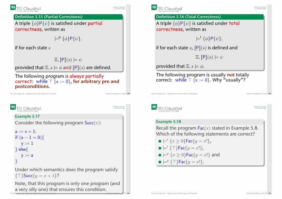
5 Hoare Calculus5.3 Hoare Logic
Definition 5.15 (Partial Correctness)
A triple {φ}P{ψ} is satisfied under partialcorrectness, written as
|=p {φ}P{ψ},
if for each state s
Z, [[P]](s) |= ψ
provided that Z, s |= φ and [[P]](s) are defined.
The following program is always partiallycorrect: while > {x := 0}, for arbitrary pre andpostconditions.
Prof. Dr. Jürgen Dix · Department of Informatics, TU Clausthal Artificial Intelligence, SS 09 389
5 Hoare Calculus5.3 Hoare Logic
Definition 5.16 (Total Correctness)
A triple {φ}P{ψ} is satisfied under totalcorrectness, written as
|=t {φ}P{ψ},
if for each state s, [[P]](s) is defined and
Z, [[P]](s) |= ψ
provided that Z, s |= φ.
The following program is usually not totallycorrect: while > {x := 0}. Why “usually”?
Prof. Dr. Jürgen Dix · Department of Informatics, TU Clausthal Artificial Intelligence, SS 09 390
5 Hoare Calculus5.3 Hoare Logic
Example 5.17
Consider the following program Succ(x):
a := x + 1;if (a− 1 = 0){
y := 1} else{
y := a}
Under which semantics does the program satisfy{>}Succ{y = x+ 1}?Note, that this program is only one program (anda very silly one) that ensures this condition.
Prof. Dr. Jürgen Dix · Department of Informatics, TU Clausthal Artificial Intelligence, SS 09 391
5 Hoare Calculus5.3 Hoare Logic
Example 5.18
Recall the program Fac(x) stated in Example 5.8.Which of the following statements are correct?|=t {x ≥ 0}Fac{y = x!},|=t {>}Fac{y = x!},|=p {x ≥ 0}Fac{y = x!} and|=p {>}Fac{y = x!}.
Prof. Dr. Jürgen Dix · Department of Informatics, TU Clausthal Artificial Intelligence, SS 09 392
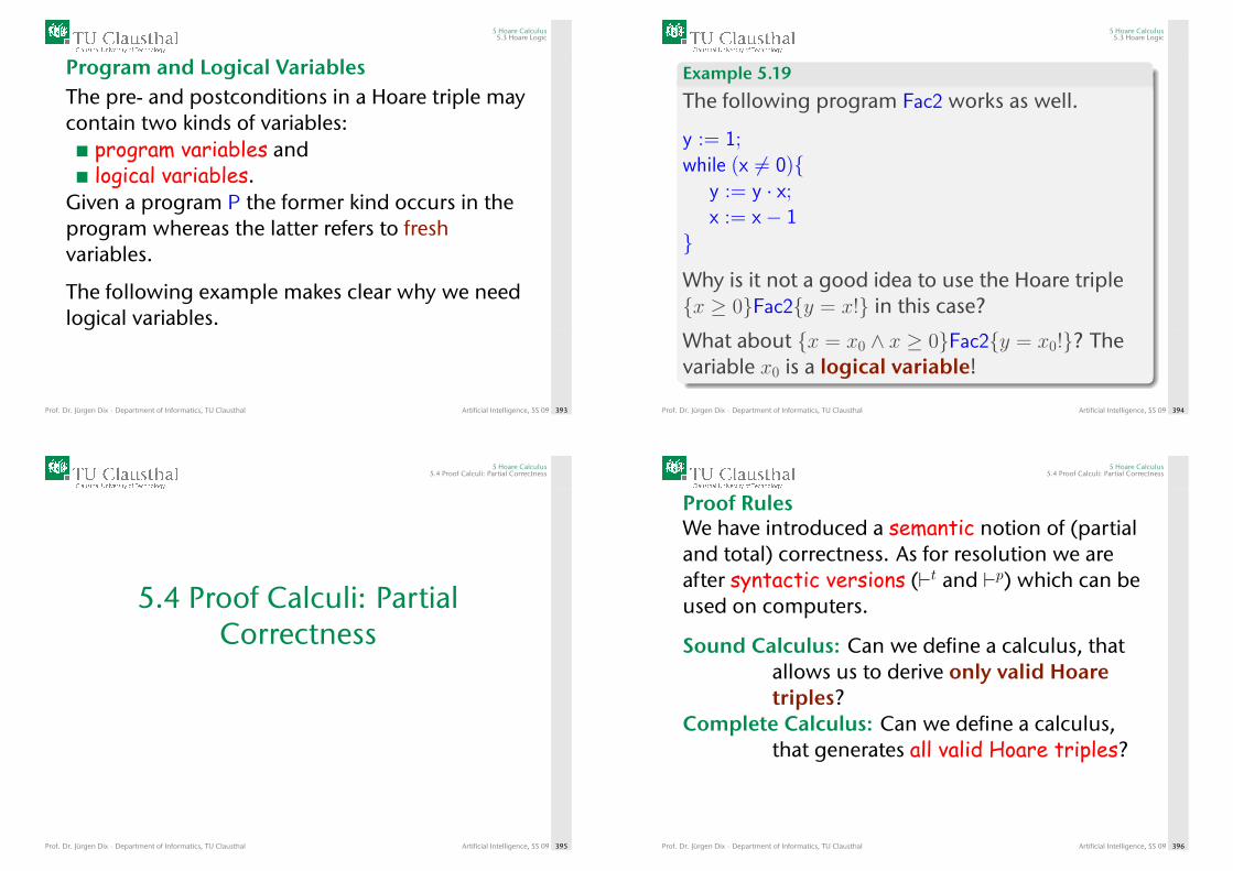
5 Hoare Calculus5.3 Hoare Logic
Program and Logical VariablesThe pre- and postconditions in a Hoare triple maycontain two kinds of variables:
program variables andlogical variables.
Given a program P the former kind occurs in theprogram whereas the latter refers to freshvariables.
The following example makes clear why we needlogical variables.
Prof. Dr. Jürgen Dix · Department of Informatics, TU Clausthal Artificial Intelligence, SS 09 393
5 Hoare Calculus5.3 Hoare Logic
Example 5.19
The following program Fac2 works as well.
y := 1;while (x 6= 0){
y := y · x;x := x− 1
}
Why is it not a good idea to use the Hoare triple{x ≥ 0}Fac2{y = x!} in this case?
What about {x = x0 ∧ x ≥ 0}Fac2{y = x0!}? Thevariable x0 is a logical variable!
Prof. Dr. Jürgen Dix · Department of Informatics, TU Clausthal Artificial Intelligence, SS 09 394
5 Hoare Calculus5.4 Proof Calculi: Partial Correctness
5.4 Proof Calculi: PartialCorrectness
Prof. Dr. Jürgen Dix · Department of Informatics, TU Clausthal Artificial Intelligence, SS 09 395
5 Hoare Calculus5.4 Proof Calculi: Partial Correctness
Proof RulesWe have introduced a semantic notion of (partialand total) correctness. As for resolution we areafter syntactic versions (`t and `p) which can beused on computers.
Sound Calculus: Can we define a calculus, thatallows us to derive only valid Hoaretriples?
Complete Calculus: Can we define a calculus,that generates all valid Hoare triples?
Prof. Dr. Jürgen Dix · Department of Informatics, TU Clausthal Artificial Intelligence, SS 09 396
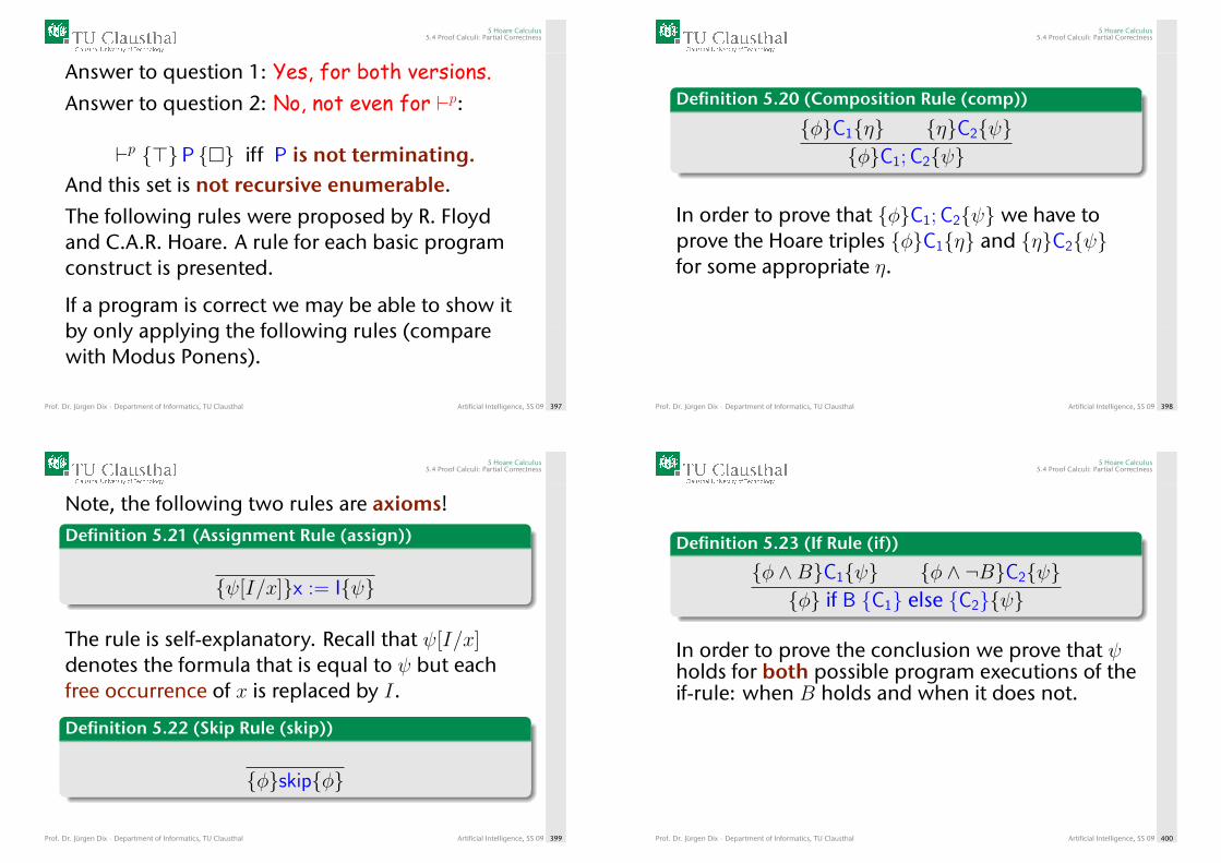
5 Hoare Calculus5.4 Proof Calculi: Partial Correctness
Answer to question 1: Yes, for both versions.Answer to question 2: No, not even for `p:
`p {>}P {�} iff P is not terminating.And this set is not recursive enumerable.
The following rules were proposed by R. Floydand C.A.R. Hoare. A rule for each basic programconstruct is presented.
If a program is correct we may be able to show itby only applying the following rules (comparewith Modus Ponens).
Prof. Dr. Jürgen Dix · Department of Informatics, TU Clausthal Artificial Intelligence, SS 09 397
5 Hoare Calculus5.4 Proof Calculi: Partial Correctness
Definition 5.20 (Composition Rule (comp))
{φ}C1{η} {η}C2{ψ}{φ}C1; C2{ψ}
In order to prove that {φ}C1; C2{ψ} we have toprove the Hoare triples {φ}C1{η} and {η}C2{ψ}for some appropriate η.
Prof. Dr. Jürgen Dix · Department of Informatics, TU Clausthal Artificial Intelligence, SS 09 398
5 Hoare Calculus5.4 Proof Calculi: Partial Correctness
Note, the following two rules are axioms!Definition 5.21 (Assignment Rule (assign))
{ψ[I/x]}x := I{ψ}
The rule is self-explanatory. Recall that ψ[I/x]denotes the formula that is equal to ψ but eachfree occurrence of x is replaced by I.
Definition 5.22 (Skip Rule (skip))
{φ}skip{φ}
Prof. Dr. Jürgen Dix · Department of Informatics, TU Clausthal Artificial Intelligence, SS 09 399
5 Hoare Calculus5.4 Proof Calculi: Partial Correctness
Definition 5.23 (If Rule (if))
{φ ∧B}C1{ψ} {φ ∧ ¬B}C2{ψ}{φ} if B {C1} else {C2}{ψ}
In order to prove the conclusion we prove that ψholds for both possible program executions of theif-rule: when B holds and when it does not.
Prof. Dr. Jürgen Dix · Department of Informatics, TU Clausthal Artificial Intelligence, SS 09 400
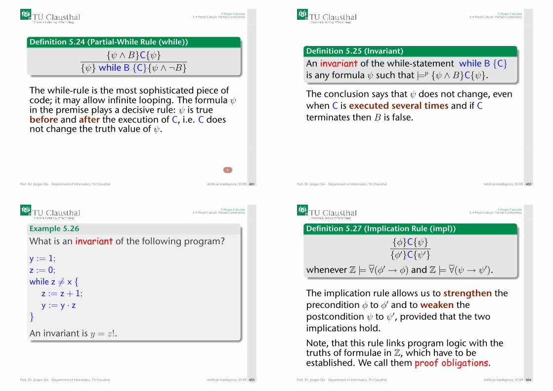
5 Hoare Calculus5.4 Proof Calculi: Partial Correctness
Definition 5.24 (Partial-While Rule (while))
{ψ ∧B}C{ψ}{ψ} while B {C}{ψ ∧ ¬B}
The while-rule is the most sophisticated piece ofcode; it may allow infinite looping. The formula ψin the premise plays a decisive rule: ψ is truebefore and after the execution of C, i.e. C doesnot change the truth value of ψ.
Prof. Dr. Jürgen Dix · Department of Informatics, TU Clausthal Artificial Intelligence, SS 09 401
5 Hoare Calculus5.4 Proof Calculi: Partial Correctness
Definition 5.25 (Invariant)
An invariant of the while-statement while B {C}is any formula ψ such that |=p {ψ ∧B}C{ψ}.
The conclusion says that ψ does not change, evenwhen C is executed several times and if Cterminates then B is false.
Prof. Dr. Jürgen Dix · Department of Informatics, TU Clausthal Artificial Intelligence, SS 09 402
5 Hoare Calculus5.4 Proof Calculi: Partial Correctness
Example 5.26
What is an invariant of the following program?
y := 1;z := 0;while z 6= x {
z := z + 1;y := y · z
}
An invariant is y = z!.
Prof. Dr. Jürgen Dix · Department of Informatics, TU Clausthal Artificial Intelligence, SS 09 403
5 Hoare Calculus5.4 Proof Calculi: Partial Correctness
Definition 5.27 (Implication Rule (impl))
{φ}C{ψ}{φ′}C{ψ′}
whenever Z |= ∀(φ′ → φ) and Z |= ∀(ψ → ψ′).
The implication rule allows us to strengthen theprecondition φ to φ′ and to weaken thepostcondition ψ to ψ′, provided that the twoimplications hold.
Note, that this rule links program logic with thetruths of formulae in Z, which have to beestablished. We call them proof obligations.
Prof. Dr. Jürgen Dix · Department of Informatics, TU Clausthal Artificial Intelligence, SS 09 404
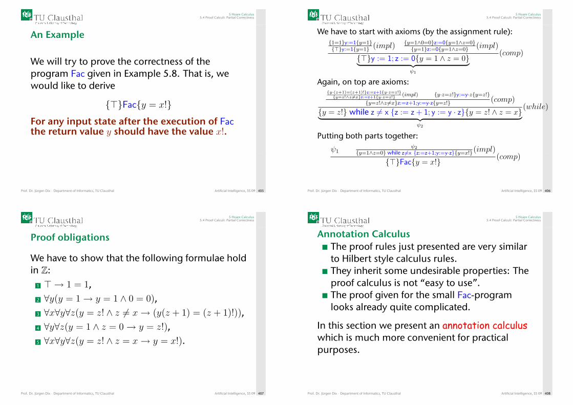
5 Hoare Calculus5.4 Proof Calculi: Partial Correctness
An Example
We will try to prove the correctness of theprogram Fac given in Example 5.8. That is, wewould like to derive
{>}Fac{y = x!}
For any input state after the execution of Facthe return value y should have the value x!.
Prof. Dr. Jürgen Dix · Department of Informatics, TU Clausthal Artificial Intelligence, SS 09 405
5 Hoare Calculus5.4 Proof Calculi: Partial Correctness
We have to start with axioms (by the assignment rule):{1=1}y:=1{y=1}{>}y:=1{y=1} (impl) {y=1∧0=0}z:=0{y=1∧z=0}
{y=1}z:=0{y=1∧z=0} (impl)
{>}y := 1; z := 0{y = 1 ∧ z = 0}︸ ︷︷ ︸ψ1
(comp)
Again, on top are axioms:{y·(z+1)=(z+1)!}z:=z+1{y·z=z!}{y=z!∧z 6=x}z:=z+1{y·z=z!} (impl) {y·z=z!}y:=y·z{y=z!}
{y=z!∧z 6=x}z:=z+1;y:=y·z{y=z!} (comp)
{y = z!} while z 6= x {z := z + 1; y := y · z}{y = z! ∧ z = x}︸ ︷︷ ︸ψ2
(while)
Putting both parts together:
ψ1ψ2
{y=1∧z=0} while z 6=x {z:=z+1;y:=y·z}{y=x!}(impl)
{>}Fac{y = x!}(comp)
Prof. Dr. Jürgen Dix · Department of Informatics, TU Clausthal Artificial Intelligence, SS 09 406
5 Hoare Calculus5.4 Proof Calculi: Partial Correctness
Proof obligations
We have to show that the following formulae holdin Z:
1 > → 1 = 1,2 ∀y(y = 1→ y = 1 ∧ 0 = 0),3 ∀x∀y∀z(y = z! ∧ z 6= x→ (y(z + 1) = (z + 1)!)),4 ∀y∀z(y = 1 ∧ z = 0→ y = z!),5 ∀x∀y∀z(y = z! ∧ z = x→ y = x!).
Prof. Dr. Jürgen Dix · Department of Informatics, TU Clausthal Artificial Intelligence, SS 09 407
5 Hoare Calculus5.4 Proof Calculi: Partial Correctness
Annotation CalculusThe proof rules just presented are very similarto Hilbert style calculus rules.They inherit some undesirable properties: Theproof calculus is not “easy to use”.The proof given for the small Fac-programlooks already quite complicated.
In this section we present an annotation calculuswhich is much more convenient for practicalpurposes.
Prof. Dr. Jürgen Dix · Department of Informatics, TU Clausthal Artificial Intelligence, SS 09 408
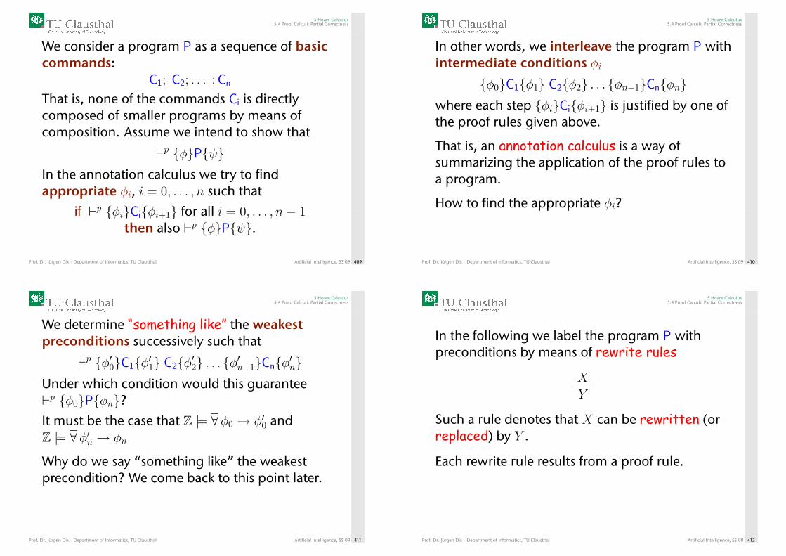
5 Hoare Calculus5.4 Proof Calculi: Partial Correctness
We consider a program P as a sequence of basiccommands:
C1; C2; . . . ; Cn
That is, none of the commands Ci is directlycomposed of smaller programs by means ofcomposition. Assume we intend to show that
`p {φ}P{ψ}In the annotation calculus we try to findappropriate φi, i = 0, . . . , n such that
if `p {φi}Ci{φi+1} for all i = 0, . . . , n− 1then also `p {φ}P{ψ}.
Prof. Dr. Jürgen Dix · Department of Informatics, TU Clausthal Artificial Intelligence, SS 09 409
5 Hoare Calculus5.4 Proof Calculi: Partial Correctness
In other words, we interleave the program P withintermediate conditions φi
{φ0}C1{φ1} C2{φ2} . . . {φn−1}Cn{φn}where each step {φi}Ci{φi+1} is justified by one ofthe proof rules given above.
That is, an annotation calculus is a way ofsummarizing the application of the proof rules toa program.
How to find the appropriate φi?
Prof. Dr. Jürgen Dix · Department of Informatics, TU Clausthal Artificial Intelligence, SS 09 410
5 Hoare Calculus5.4 Proof Calculi: Partial Correctness
We determine “something like” the weakestpreconditions successively such that
`p {φ′0}C1{φ′1} C2{φ′2} . . . {φ′n−1}Cn{φ′n}Under which condition would this guarantee`p {φ0}P{φn}?It must be the case that Z |= ∀φ0 → φ′0 andZ |= ∀φ′n → φn
Why do we say “something like” the weakestprecondition? We come back to this point later.
Prof. Dr. Jürgen Dix · Department of Informatics, TU Clausthal Artificial Intelligence, SS 09 411
5 Hoare Calculus5.4 Proof Calculi: Partial Correctness
In the following we label the program P withpreconditions by means of rewrite rules
X
Y
Such a rule denotes that X can be rewritten (orreplaced) by Y .
Each rewrite rule results from a proof rule.
Prof. Dr. Jürgen Dix · Department of Informatics, TU Clausthal Artificial Intelligence, SS 09 412
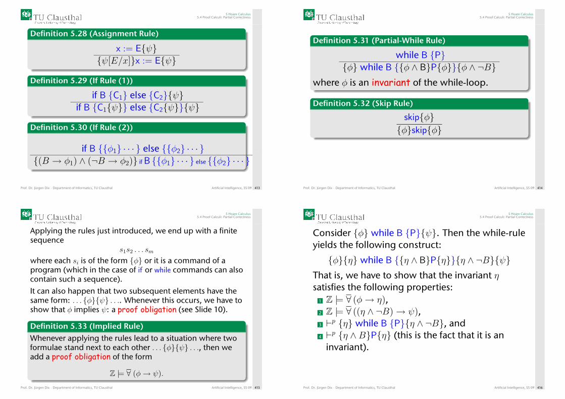
5 Hoare Calculus5.4 Proof Calculi: Partial Correctness
Definition 5.28 (Assignment Rule)
x := E{ψ}{ψ[E/x]}x := E{ψ}
Definition 5.29 (If Rule (1))
if B {C1} else {C2}{ψ}if B {C1{ψ}} else {C2{ψ}}{ψ}
Definition 5.30 (If Rule (2))
if B {{φ1} · · · } else {{φ2} · · · }{(B → φ1) ∧ (¬B → φ2)} if B {{φ1} · · · } else {{φ2} · · · }
Prof. Dr. Jürgen Dix · Department of Informatics, TU Clausthal Artificial Intelligence, SS 09 413
5 Hoare Calculus5.4 Proof Calculi: Partial Correctness
Definition 5.31 (Partial-While Rule)
while B {P}{φ} while B {{φ ∧ B}P{φ}}{φ ∧ ¬B}
where φ is an invariant of the while-loop.
Definition 5.32 (Skip Rule)
skip{φ}{φ}skip{φ}
Prof. Dr. Jürgen Dix · Department of Informatics, TU Clausthal Artificial Intelligence, SS 09 414
5 Hoare Calculus5.4 Proof Calculi: Partial Correctness
Applying the rules just introduced, we end up with a finitesequence
s1s2 . . . sm
where each si is of the form {φ} or it is a command of aprogram (which in the case of if or while commands can alsocontain such a sequence).It can also happen that two subsequent elements have thesame form: . . . {φ}{ψ} . . .. Whenever this occurs, we have toshow that φ implies ψ: a proof obligation (see Slide 10).
Definition 5.33 (Implied Rule)Whenever applying the rules lead to a situation where twoformulae stand next to each other . . . {φ}{ψ} . . ., then weadd a proof obligation of the form
Z |= ∀ (φ→ ψ).
Prof. Dr. Jürgen Dix · Department of Informatics, TU Clausthal Artificial Intelligence, SS 09 415
5 Hoare Calculus5.4 Proof Calculi: Partial Correctness
Consider {φ} while B {P}{ψ}. Then the while-ruleyields the following construct:
{φ}{η} while B {{η ∧ B}P{η}}{η ∧ ¬B}{ψ}That is, we have to show that the invariant ηsatisfies the following properties:
1 Z |= ∀ (φ→ η),2 Z |= ∀ ((η ∧ ¬B)→ ψ),3 `p {η} while B {P}{η ∧ ¬B}, and4 `p {η ∧B}P{η} (this is the fact that it is an
invariant).
Prof. Dr. Jürgen Dix · Department of Informatics, TU Clausthal Artificial Intelligence, SS 09 416
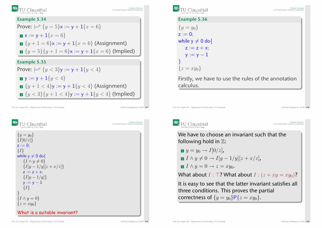
5 Hoare Calculus5.4 Proof Calculi: Partial Correctness
Example 5.34
Prove: |=p {y = 5}x := y + 1{x = 6}1 x := y + 1{x = 6}2 {y + 1 = 6}x := y + 1{x = 6} (Assignment)3 {y = 5}{y + 1 = 6}x := y + 1{x = 6} (Implied)
Example 5.35
Prove: |=p {y < 3}y := y + 1{y < 4}1 y := y + 1{y < 4}2 {y + 1 < 4}y := y + 1{y < 4} (Assignment)3 {y < 3}{y + 1 < 4}y := y + 1{y < 4} (Implied)
Prof. Dr. Jürgen Dix · Department of Informatics, TU Clausthal Artificial Intelligence, SS 09 417
5 Hoare Calculus5.4 Proof Calculi: Partial Correctness
Example 5.36
{y = y0}z := 0;while y 6= 0 do{
z := z + x;y := y − 1
}{z = xy0}
Firstly, we have to use the rules of the annotationcalculus.
Prof. Dr. Jürgen Dix · Department of Informatics, TU Clausthal Artificial Intelligence, SS 09 418
5 Hoare Calculus5.4 Proof Calculi: Partial Correctness
{y = y0}{I[0/z]}z := 0;{I}while y 6= 0 do{{I ∧ y 6= 0}{I[y − 1/y][z + x/z]}z := z + x;{I[y − 1/y]}y := y − 1{I}
}{I ∧ y = 0}{z = xy0}
What is a suitable invariant?
Prof. Dr. Jürgen Dix · Department of Informatics, TU Clausthal Artificial Intelligence, SS 09 419
5 Hoare Calculus5.4 Proof Calculi: Partial Correctness
We have to choose an invariant such that thefollowing hold in Z:
1 y = y0 → I[0/z],2 I ∧ y 6= 0→ I[y − 1/y][z + x/z],3 I ∧ y = 0→ z = xy0.
What about I : >? What about I : (z + xy = xy0)?
It is easy to see that the latter invariant satisfies allthree conditions. This proves the partialcorrectness of {y = y0}P{z = xy0}.
Prof. Dr. Jürgen Dix · Department of Informatics, TU Clausthal Artificial Intelligence, SS 09 420
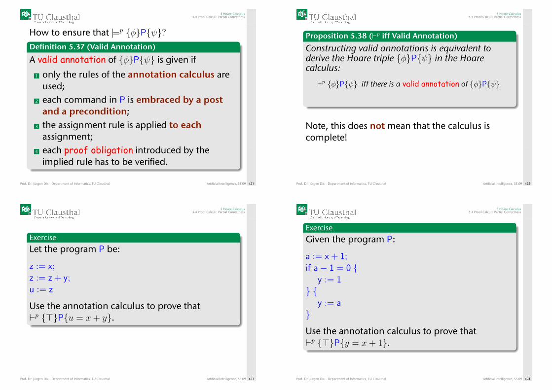
5 Hoare Calculus5.4 Proof Calculi: Partial Correctness
How to ensure that |=p {φ}P{ψ}?Definition 5.37 (Valid Annotation)
A valid annotation of {φ}P{ψ} is given if
1 only the rules of the annotation calculus areused;
2 each command in P is embraced by a postand a precondition;
3 the assignment rule is applied to eachassignment;
4 each proof obligation introduced by theimplied rule has to be verified.
Prof. Dr. Jürgen Dix · Department of Informatics, TU Clausthal Artificial Intelligence, SS 09 421
5 Hoare Calculus5.4 Proof Calculi: Partial Correctness
Proposition 5.38 (`p iff Valid Annotation)
Constructing valid annotations is equivalent toderive the Hoare triple {φ}P{ψ} in the Hoarecalculus:
`p {φ}P{ψ} iff there is a valid annotation of {φ}P{ψ}.
Note, this does not mean that the calculus iscomplete!
Prof. Dr. Jürgen Dix · Department of Informatics, TU Clausthal Artificial Intelligence, SS 09 422
5 Hoare Calculus5.4 Proof Calculi: Partial Correctness
Exercise
Let the program P be:
z := x;z := z + y;u := z
Use the annotation calculus to prove that`p {>}P{u = x+ y}.
Prof. Dr. Jürgen Dix · Department of Informatics, TU Clausthal Artificial Intelligence, SS 09 423
5 Hoare Calculus5.4 Proof Calculi: Partial Correctness
Exercise
Given the program P:
a := x + 1;if a− 1 = 0 {
y := 1} {
y := a}
Use the annotation calculus to prove that`p {>}P{y = x+ 1}.
Prof. Dr. Jürgen Dix · Department of Informatics, TU Clausthal Artificial Intelligence, SS 09 424
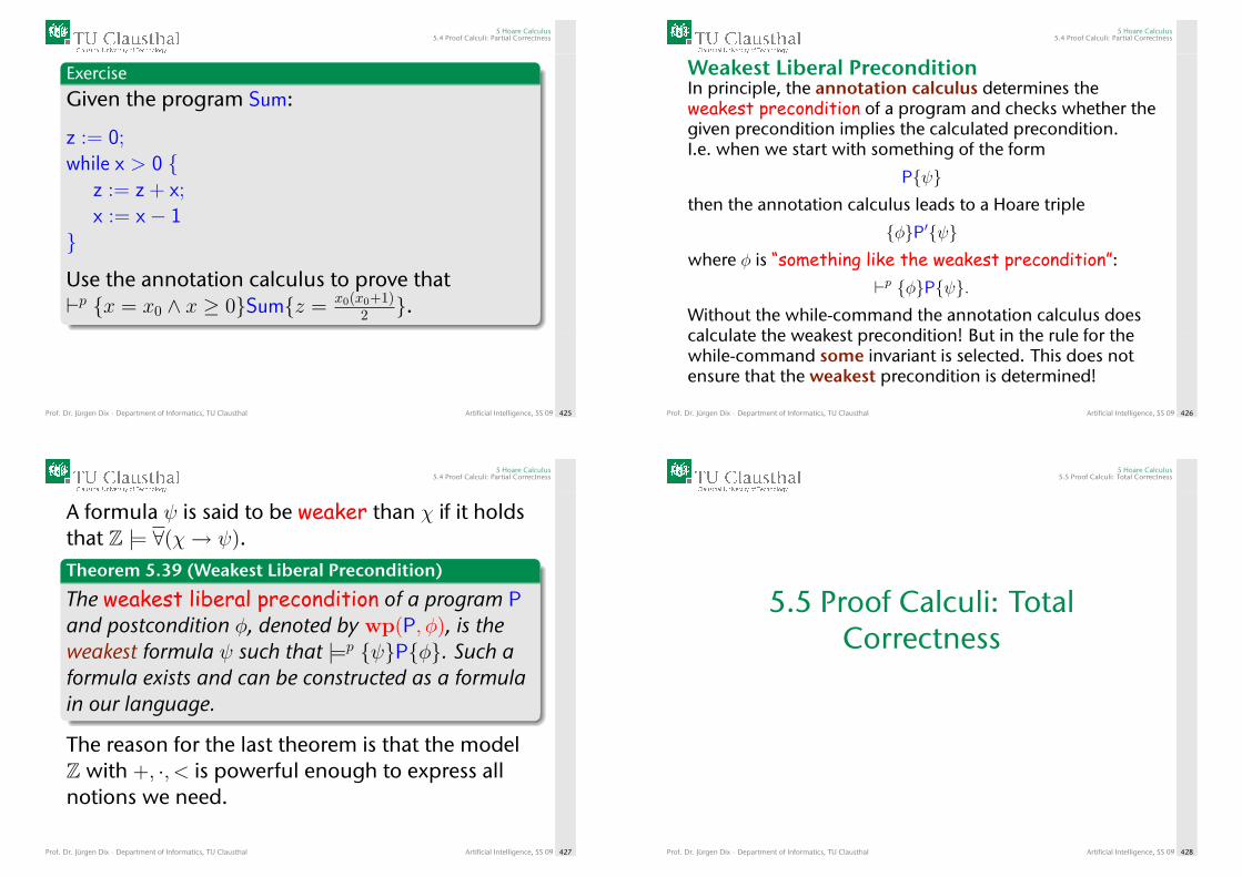
5 Hoare Calculus5.4 Proof Calculi: Partial Correctness
Exercise
Given the program Sum:
z := 0;while x > 0 {
z := z + x;x := x− 1
}
Use the annotation calculus to prove that`p {x = x0 ∧ x ≥ 0}Sum{z = x0(x0+1)
2 }.
Prof. Dr. Jürgen Dix · Department of Informatics, TU Clausthal Artificial Intelligence, SS 09 425
5 Hoare Calculus5.4 Proof Calculi: Partial Correctness
Weakest Liberal PreconditionIn principle, the annotation calculus determines theweakest precondition of a program and checks whether thegiven precondition implies the calculated precondition.I.e. when we start with something of the form
P{ψ}then the annotation calculus leads to a Hoare triple
{φ}P′{ψ}where φ is “something like the weakest precondition”:
`p {φ}P{ψ}.Without the while-command the annotation calculus doescalculate the weakest precondition! But in the rule for thewhile-command some invariant is selected. This does notensure that the weakest precondition is determined!
Prof. Dr. Jürgen Dix · Department of Informatics, TU Clausthal Artificial Intelligence, SS 09 426
5 Hoare Calculus5.4 Proof Calculi: Partial Correctness
A formula ψ is said to be weaker than χ if it holdsthat Z |= ∀(χ→ ψ).Theorem 5.39 (Weakest Liberal Precondition)
The weakest liberal precondition of a program Pand postcondition φ, denoted by wp(P, φ), is theweakest formula ψ such that |=p {ψ}P{φ}. Such aformula exists and can be constructed as a formulain our language.
The reason for the last theorem is that the modelZ with +, ·, < is powerful enough to express allnotions we need.
Prof. Dr. Jürgen Dix · Department of Informatics, TU Clausthal Artificial Intelligence, SS 09 427
5 Hoare Calculus5.5 Proof Calculi: Total Correctness
5.5 Proof Calculi: TotalCorrectness
Prof. Dr. Jürgen Dix · Department of Informatics, TU Clausthal Artificial Intelligence, SS 09 428
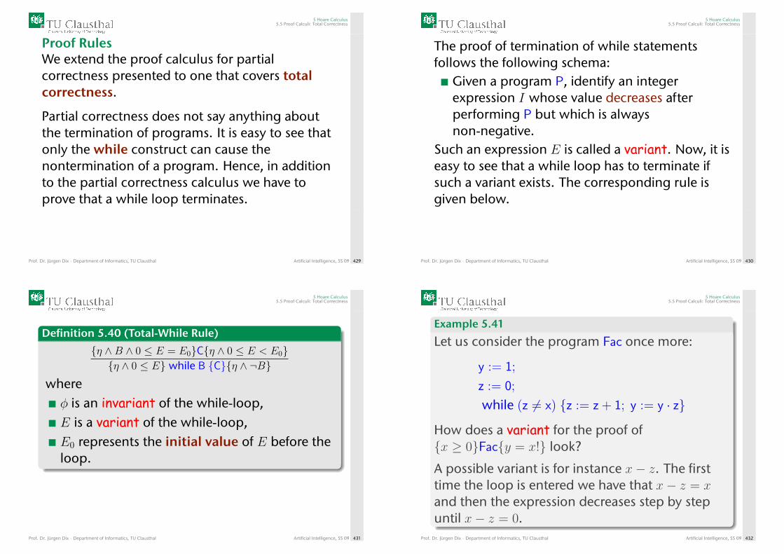
5 Hoare Calculus5.5 Proof Calculi: Total Correctness
Proof RulesWe extend the proof calculus for partialcorrectness presented to one that covers totalcorrectness.
Partial correctness does not say anything aboutthe termination of programs. It is easy to see thatonly the while construct can cause thenontermination of a program. Hence, in additionto the partial correctness calculus we have toprove that a while loop terminates.
Prof. Dr. Jürgen Dix · Department of Informatics, TU Clausthal Artificial Intelligence, SS 09 429
5 Hoare Calculus5.5 Proof Calculi: Total Correctness
The proof of termination of while statementsfollows the following schema:
Given a program P, identify an integerexpression I whose value decreases afterperforming P but which is alwaysnon-negative.
Such an expression E is called a variant. Now, it iseasy to see that a while loop has to terminate ifsuch a variant exists. The corresponding rule isgiven below.
Prof. Dr. Jürgen Dix · Department of Informatics, TU Clausthal Artificial Intelligence, SS 09 430
5 Hoare Calculus5.5 Proof Calculi: Total Correctness
Definition 5.40 (Total-While Rule)
{η ∧B ∧ 0 ≤ E = E0}C{η ∧ 0 ≤ E < E0}{η ∧ 0 ≤ E} while B {C}{η ∧ ¬B}
whereφ is an invariant of the while-loop,E is a variant of the while-loop,E0 represents the initial value of E before theloop.
Prof. Dr. Jürgen Dix · Department of Informatics, TU Clausthal Artificial Intelligence, SS 09 431
5 Hoare Calculus5.5 Proof Calculi: Total Correctness
Example 5.41
Let us consider the program Fac once more:
y := 1;
z := 0;
while (z 6= x) {z := z + 1; y := y · z}
How does a variant for the proof of{x ≥ 0}Fac{y = x!} look?
A possible variant is for instance x− z. The firsttime the loop is entered we have that x− z = x
and then the expression decreases step by stepuntil x− z = 0.
Prof. Dr. Jürgen Dix · Department of Informatics, TU Clausthal Artificial Intelligence, SS 09 432
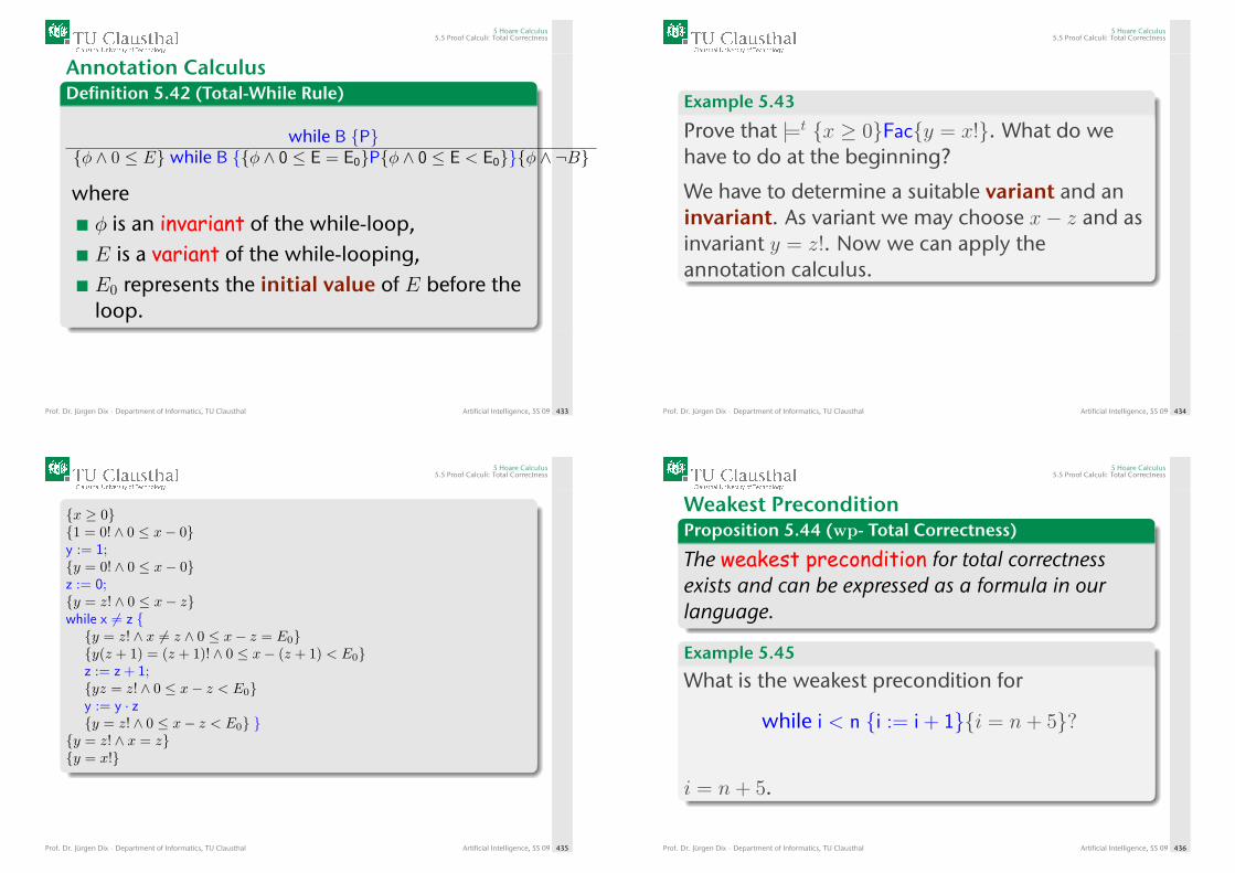
5 Hoare Calculus5.5 Proof Calculi: Total Correctness
Annotation CalculusDefinition 5.42 (Total-While Rule)
while B {P}{φ ∧ 0 ≤ E} while B {{φ ∧ 0 ≤ E = E0}P{φ ∧ 0 ≤ E < E0}}{φ ∧ ¬B}
whereφ is an invariant of the while-loop,E is a variant of the while-looping,E0 represents the initial value of E before theloop.
Prof. Dr. Jürgen Dix · Department of Informatics, TU Clausthal Artificial Intelligence, SS 09 433
5 Hoare Calculus5.5 Proof Calculi: Total Correctness
Example 5.43
Prove that |=t {x ≥ 0}Fac{y = x!}. What do wehave to do at the beginning?
We have to determine a suitable variant and aninvariant. As variant we may choose x− z and asinvariant y = z!. Now we can apply theannotation calculus.
Prof. Dr. Jürgen Dix · Department of Informatics, TU Clausthal Artificial Intelligence, SS 09 434
5 Hoare Calculus5.5 Proof Calculi: Total Correctness
{x ≥ 0}{1 = 0! ∧ 0 ≤ x− 0}y := 1;{y = 0! ∧ 0 ≤ x− 0}z := 0;{y = z! ∧ 0 ≤ x− z}while x 6= z {{y = z! ∧ x 6= z ∧ 0 ≤ x− z = E0}{y(z + 1) = (z + 1)! ∧ 0 ≤ x− (z + 1) < E0}z := z + 1;{yz = z! ∧ 0 ≤ x− z < E0}y := y · z{y = z! ∧ 0 ≤ x− z < E0} }
{y = z! ∧ x = z}{y = x!}
Prof. Dr. Jürgen Dix · Department of Informatics, TU Clausthal Artificial Intelligence, SS 09 435
5 Hoare Calculus5.5 Proof Calculi: Total Correctness
Weakest PreconditionProposition 5.44 (wp- Total Correctness)
The weakest precondition for total correctnessexists and can be expressed as a formula in ourlanguage.
Example 5.45
What is the weakest precondition for
while i < n {i := i + 1}{i = n+ 5}?
i = n+ 5.
Prof. Dr. Jürgen Dix · Department of Informatics, TU Clausthal Artificial Intelligence, SS 09 436
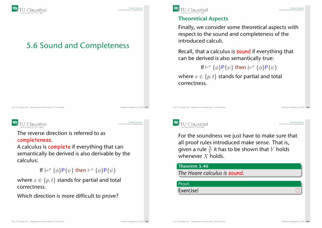
5 Hoare Calculus5.6 Sound and Completeness
5.6 Sound and Completeness
Prof. Dr. Jürgen Dix · Department of Informatics, TU Clausthal Artificial Intelligence, SS 09 437
5 Hoare Calculus5.6 Sound and Completeness
Theoretical Aspects
Finally, we consider some theoretical aspects withrespect to the sound and completeness of theintroduced calculi.
Recall, that a calculus is sound if everything thatcan be derived is also semantically true:
If `x {φ}P{ψ} then |=x {φ}P{ψ}where x ∈ {p, t} stands for partial and totalcorrectness.
Prof. Dr. Jürgen Dix · Department of Informatics, TU Clausthal Artificial Intelligence, SS 09 438
5 Hoare Calculus5.6 Sound and Completeness
The reverse direction is referred to ascompleteness.A calculus is complete if everything that cansemantically be derived is also derivable by thecalculus:
If |=x {φ}P{ψ} then `x {φ}P{ψ}
where x ∈ {p, t} stands for partial and totalcorrectness.
Which direction is more difficult to prove?
Prof. Dr. Jürgen Dix · Department of Informatics, TU Clausthal Artificial Intelligence, SS 09 439
5 Hoare Calculus5.6 Sound and Completeness
For the soundness we just have to make sure thatall proof rules introduced make sense. That is,given a rule X
Y it has to be shown that Y holdswhenever X holds.
Theorem 5.46
The Hoare calculus is sound.
Proof.
Exercise!
Prof. Dr. Jürgen Dix · Department of Informatics, TU Clausthal Artificial Intelligence, SS 09 440
5 Hoare Calculus5.6 Sound and Completeness
Theorem 5.47
The Hoare calculus is complete.
The Hoare calculus contains axioms and rulesthat require to determine whether certainformulae (proof obligations) are true in Z.The theory of Z is undecidable.Thus any re axiomatization of Z is incomplete.However, most proof obligations occurring inpractice can be checked by theorem provers.
Prof. Dr. Jürgen Dix · Department of Informatics, TU Clausthal Artificial Intelligence, SS 09 441
6 Knowledge Engineering: FOL
6. Knowledge Engineering: FOL6 Knowledge Engineering: FOL
First Order LogicSit-CalculusThe BlocksworldHigher order logic
Prof. Dr. Jürgen Dix · Department of Informatics, TU Clausthal Artificial Intelligence, SS 09 442
6 Knowledge Engineering: FOL
Content of this chapter:
FOL: While sentential logic SL has some nice features,it is quite restricted in expressivity. First orderlogic (FOL) is an extension of SL which allows usto express much more in a succinct way.
SIT-calculus: The Situation Calculus, introduced by JohnMcCarthy, is a special method for using FOL toexpress the dynamics of an agent. Applyingactions to the world leads to a series ofsuccessor worlds that can be represented withspecial FOL terms.
Prof. Dr. Jürgen Dix · Department of Informatics, TU Clausthal Artificial Intelligence, SS 09 443
6 Knowledge Engineering: FOL
Content of this chapter (2):
Blocksworld: We consider the blocksworld scenario anddiscuss how to formalize that with FOL.
HOL: Finally, we give an outlook to higher orderlogics (HOL), in particular to second order logic.While we can express much more than in 1storder logic, the price we have to pay is that thereis no correct and complete calculus.
Declarative: In this chapter we only consider the questionHow to use FOL to model the world? We arenot concerned with deriving new informationor with implementing FOL. This will be done inthe next chapter.
Prof. Dr. Jürgen Dix · Department of Informatics, TU Clausthal Artificial Intelligence, SS 09 444
6 Knowledge Engineering: FOL6.1 First Order Logic
6.1 First Order Logic
Prof. Dr. Jürgen Dix · Department of Informatics, TU Clausthal Artificial Intelligence, SS 09 445
6 Knowledge Engineering: FOL6.1 First Order Logic
Definition 6.1 (First order logic LFOL, L ⊆ LFOL)
The language LFOL of first order logic (Prädikatenlogikerster Stufe) is:
x, y, z, x1, x2, . . . , xn, . . .: a countable set Var of variablesfor each k ∈ N0: P k
1 , Pk2 , . . . , P
kn , . . . a countable set
Predk of k-dimensional predicate symbols (the0-dimensional predicate symbols are the propositionallogic constants from At of LSL, including �, >).for each k ∈ N0: fk1 , f
k2 , . . . , f
kn , . . . a countable set
Functk of k-dimensional function symbols.¬, ∧, ∨,→: the sentential connectives.(, ): the parentheses.∀, ∃: the quantifiers.
Prof. Dr. Jürgen Dix · Department of Informatics, TU Clausthal Artificial Intelligence, SS 09 446
6 Knowledge Engineering: FOL6.1 First Order Logic
Definition (continued)The 0-dimensional function symbols are called individuumconstants – we leave out the parentheses. In general wewill need – as in propositional logic – only a certain subsetof the predicate or function symbols.
These define a language L ⊆ LFOL (analogously todefinition 4.1 on page 2). The used set of predicate andfunction symbols is also called signature Σ.
Prof. Dr. Jürgen Dix · Department of Informatics, TU Clausthal Artificial Intelligence, SS 09 447
6 Knowledge Engineering: FOL6.1 First Order Logic
Definition (continued)
The concept of an L-term t and an L-formula ϕ are definedinductively:
Term: L-terms t are defined as follows:1 each variable is a L-term.2 if fk is a k-dimensional function symbol from L and t1,
. . . ,tk are L-terms, then fk(t1, . . . , tk) is a L-term.The set of all L-terms that one can create from the setX ⊆ Var is called TermL(X) or TermΣ(X). Using X = ∅ weget the set of basic terms TermL(∅), short: TermL.
Prof. Dr. Jürgen Dix · Department of Informatics, TU Clausthal Artificial Intelligence, SS 09 448
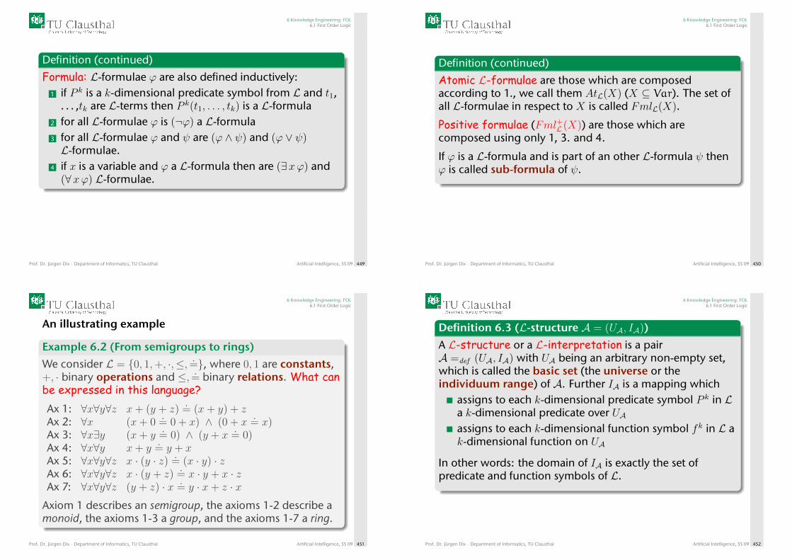
6 Knowledge Engineering: FOL6.1 First Order Logic
Definition (continued)
Formula: L-formulae ϕ are also defined inductively:1 if P k is a k-dimensional predicate symbol from L and t1,
. . . ,tk are L-terms then P k(t1, . . . , tk) is a L-formula2 for all L-formulae ϕ is (¬ϕ) a L-formula3 for all L-formulae ϕ and ψ are (ϕ ∧ ψ) and (ϕ ∨ ψ)L-formulae.
4 if x is a variable and ϕ a L-formula then are (∃xϕ) and(∀xϕ) L-formulae.
Prof. Dr. Jürgen Dix · Department of Informatics, TU Clausthal Artificial Intelligence, SS 09 449
6 Knowledge Engineering: FOL6.1 First Order Logic
Definition (continued)
Atomic L-formulae are those which are composedaccording to 1., we call them AtL(X) (X ⊆ Var). The set ofall L-formulae in respect to X is called FmlL(X).
Positive formulae (Fml+L (X)) are those which arecomposed using only 1, 3. and 4.
If ϕ is a L-formula and is part of an other L-formula ψ thenϕ is called sub-formula of ψ.
Prof. Dr. Jürgen Dix · Department of Informatics, TU Clausthal Artificial Intelligence, SS 09 450
6 Knowledge Engineering: FOL6.1 First Order Logic
An illustrating example
Example 6.2 (From semigroups to rings)
We consider L = {0, 1,+, ·,≤, .=}, where 0, 1 are constants,+, · binary operations and ≤, .= binary relations. What canbe expressed in this language?Ax 1: ∀x∀y∀z x+ (y + z)
.= (x+ y) + z
Ax 2: ∀x (x+ 0.= 0 + x) ∧ (0 + x
.= x)
Ax 3: ∀x∃y (x+ y.= 0) ∧ (y + x
.= 0)
Ax 4: ∀x∀y x+ y.= y + x
Ax 5: ∀x∀y∀z x · (y · z).= (x · y) · z
Ax 6: ∀x∀y∀z x · (y + z).= x · y + x · z
Ax 7: ∀x∀y∀z (y + z) · x .= y · x+ z · x
Axiom 1 describes an semigroup, the axioms 1-2 describe amonoid, the axioms 1-3 a group, and the axioms 1-7 a ring.
Prof. Dr. Jürgen Dix · Department of Informatics, TU Clausthal Artificial Intelligence, SS 09 451
6 Knowledge Engineering: FOL6.1 First Order Logic
Definition 6.3 (L-structure A = (UA, IA))
A L-structure or a L-interpretation is a pairA =def (UA, IA) with UA being an arbitrary non-empty set,which is called the basic set (the universe or theindividuum range) of A. Further IA is a mapping which
assigns to each k-dimensional predicate symbol P k in La k-dimensional predicate over UAassigns to each k-dimensional function symbol fk in L ak-dimensional function on UA
In other words: the domain of IA is exactly the set ofpredicate and function symbols of L.
Prof. Dr. Jürgen Dix · Department of Informatics, TU Clausthal Artificial Intelligence, SS 09 452
6 Knowledge Engineering: FOL6.1 First Order Logic
Definition (continued)The range of IA consists of the predicates and functions onUA. We write:
IA(P ) = PA, IA(f) = fA.
ϕ be a L1-formula and A =def (UA, IA) a L-structure. A iscalled matching with ϕ if IA is defined for all predicate andfunction symbols which appear in ϕ, i.e. if L1 ⊆ L.
FOL with Equality
Often, one assumes that the predicate symbol .= is built-inand interpreted by identity in all structures A:IA(
.=) = {(x, x) : x ∈ A}. In that case, .= is not listed among
the predicates in a model A.Prof. Dr. Jürgen Dix · Department of Informatics, TU Clausthal Artificial Intelligence, SS 09 453
6 Knowledge Engineering: FOL6.1 First Order Logic
Definition 6.4 (Variable assignment %)
A variable assignment % over a L-structureA = (UA, IA) is a function
% : Var → UA; x 7→ %(x).
Note that this is exactly what we called state inthe chapter about the Hoare calculus.
Prof. Dr. Jürgen Dix · Department of Informatics, TU Clausthal Artificial Intelligence, SS 09 454
6 Knowledge Engineering: FOL6.1 First Order Logic
Some structuresThe following will be explained in detail on theblackboard.
We consider L = {≤, .=} and the followingstructures
1 (Z,≤Z)2 (R,≤R)3 (Q,≤Q)4 (Q+
0 ,≤Q+0 )
State formulae in L that are true in all structures,just in some, . . . . Is there a formula φ which candistinguish between (R,≤R) and (Q,≤Q)?
Prof. Dr. Jürgen Dix · Department of Informatics, TU Clausthal Artificial Intelligence, SS 09 455
6 Knowledge Engineering: FOL6.1 First Order Logic
Some structures (2)We have seen some formulae that are true in thesestructures. Can we come up with a finiteaxiomatization?
Dense linear order without endpoints
It turns out, that the set of all formulae true in(R,≤R) coincides with the set all formulae true in(Q,≤Q). An axiomatization is given by the finiteset of formulae stating that < is a dense, linearorder without endpoints. This theory is alsocomplete.
Prof. Dr. Jürgen Dix · Department of Informatics, TU Clausthal Artificial Intelligence, SS 09 456
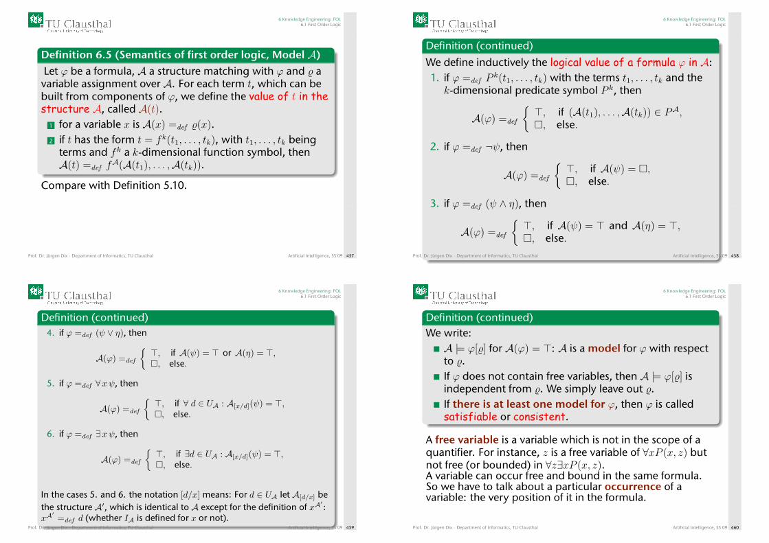
6 Knowledge Engineering: FOL6.1 First Order Logic
Definition 6.5 (Semantics of first order logic, Model A)Let ϕ be a formula, A a structure matching with ϕ and % avariable assignment over A. For each term t, which can bebuilt from components of ϕ, we define the value of t in thestructure A, called A(t).
1 for a variable x is A(x) =def %(x).2 if t has the form t = fk(t1, . . . , tk), with t1, . . . , tk being
terms and fk a k-dimensional function symbol, thenA(t) =def f
A(A(t1), . . . ,A(tk)).
Compare with Definition 5.10.
Prof. Dr. Jürgen Dix · Department of Informatics, TU Clausthal Artificial Intelligence, SS 09 457
6 Knowledge Engineering: FOL6.1 First Order Logic
Definition (continued)
We define inductively the logical value of a formula ϕ in A:1. if ϕ =def P
k(t1, . . . , tk) with the terms t1, . . . , tk and thek-dimensional predicate symbol P k, then
A(ϕ) =def
{>, if (A(t1), . . . ,A(tk)) ∈ PA,�, else.
2. if ϕ =def ¬ψ, then
A(ϕ) =def
{>, if A(ψ) = �,�, else.
3. if ϕ =def (ψ ∧ η), then
A(ϕ) =def
{>, if A(ψ) = > and A(η) = >,�, else.
Prof. Dr. Jürgen Dix · Department of Informatics, TU Clausthal Artificial Intelligence, SS 09 458
6 Knowledge Engineering: FOL6.1 First Order Logic
Definition (continued)4. if ϕ =def (ψ ∨ η), then
A(ϕ) =def
{>, if A(ψ) = > or A(η) = >,�, else.
5. if ϕ =def ∀xψ, then
A(ϕ) =def
{>, if ∀ d ∈ UA : A[x/d](ψ) = >,�, else.
6. if ϕ =def ∃xψ, then
A(ϕ) =def
{>, if ∃d ∈ UA : A[x/d](ψ) = >,�, else.
In the cases 5. and 6. the notation [d/x] means: For d ∈ UA let A[d/x] bethe structure A′, which is identical to A except for the definition of xA
′:
xA′
=def d (whether IA is defined for x or not).Prof. Dr. Jürgen Dix · Department of Informatics, TU Clausthal Artificial Intelligence, SS 09 459
6 Knowledge Engineering: FOL6.1 First Order Logic
Definition (continued)We write:A |= ϕ[%] for A(ϕ) = >: A is a model for ϕ with respectto %.If ϕ does not contain free variables, then A |= ϕ[%] isindependent from %. We simply leave out %.If there is at least one model for ϕ, then ϕ is calledsatisfiable or consistent.
A free variable is a variable which is not in the scope of aquantifier. For instance, z is a free variable of ∀xP (x, z) butnot free (or bounded) in ∀z∃xP (x, z).A variable can occur free and bound in the same formula.So we have to talk about a particular occurrence of avariable: the very position of it in the formula.
Prof. Dr. Jürgen Dix · Department of Informatics, TU Clausthal Artificial Intelligence, SS 09 460
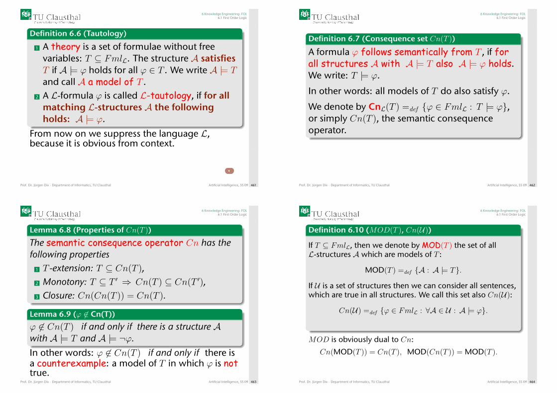
6 Knowledge Engineering: FOL6.1 First Order Logic
Definition 6.6 (Tautology)
1 A theory is a set of formulae without freevariables: T ⊆ FmlL. The structure A satisfiesT if A |= ϕ holds for all ϕ ∈ T . We write A |= Tand call A a model of T .
2 A L-formula ϕ is called L-tautology, if for allmatching L-structures A the followingholds: A |= ϕ.
From now on we suppress the language L,because it is obvious from context.
Prof. Dr. Jürgen Dix · Department of Informatics, TU Clausthal Artificial Intelligence, SS 09 461
6 Knowledge Engineering: FOL6.1 First Order Logic
Definition 6.7 (Consequence set Cn(T ))
A formula ϕ follows semantically from T , if forall structures A with A |= T also A |= ϕ holds.We write: T |= ϕ.
In other words: all models of T do also satisfy ϕ.
We denote by CnL(T ) =def {ϕ ∈ FmlL : T |= ϕ},or simply Cn(T ), the semantic consequenceoperator.
Prof. Dr. Jürgen Dix · Department of Informatics, TU Clausthal Artificial Intelligence, SS 09 462
6 Knowledge Engineering: FOL6.1 First Order Logic
Lemma 6.8 (Properties of Cn(T ))
The semantic consequence operator Cn has thefollowing properties
1 T -extension: T ⊆ Cn(T ),2 Monotony: T ⊆ T ′ ⇒ Cn(T ) ⊆ Cn(T ′),3 Closure: Cn(Cn(T )) = Cn(T ).
Lemma 6.9 (ϕ 6∈ Cn(T))
ϕ 6∈ Cn(T ) if and only if there is a structure Awith A |= T and A |= ¬ϕ.
In other words: ϕ 6∈ Cn(T ) if and only if there isa counterexample: a model of T in which ϕ is nottrue.
Prof. Dr. Jürgen Dix · Department of Informatics, TU Clausthal Artificial Intelligence, SS 09 463
6 Knowledge Engineering: FOL6.1 First Order Logic
Definition 6.10 (MOD(T ), Cn(U))
If T ⊆ FmlL, then we denote by MOD(T ) the set of allL-structures A which are models of T :
MOD(T ) =def {A : A |= T}.
If U is a set of structures then we can consider all sentences,which are true in all structures. We call this set also Cn(U):
Cn(U) =def {ϕ ∈ FmlL : ∀A ∈ U : A |= ϕ}.
MOD is obviously dual to Cn:
Cn(MOD(T )) = Cn(T ), MOD(Cn(T )) = MOD(T ).
Prof. Dr. Jürgen Dix · Department of Informatics, TU Clausthal Artificial Intelligence, SS 09 464
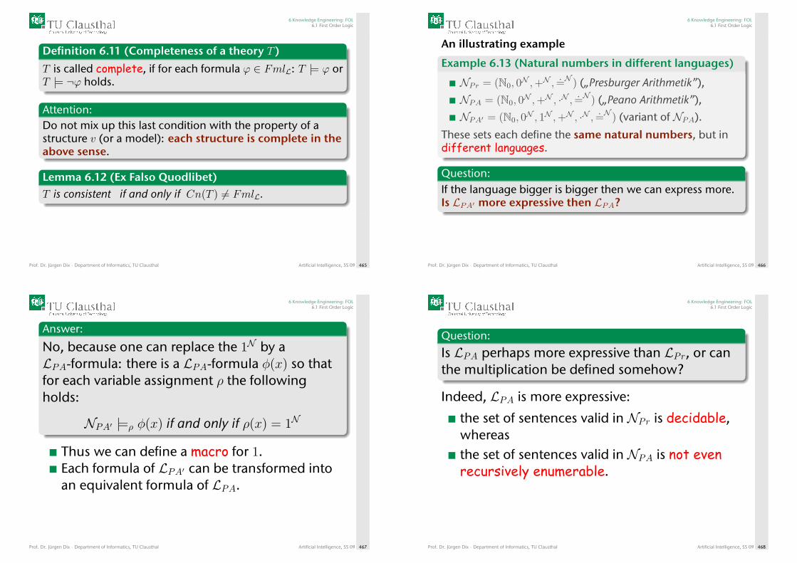
6 Knowledge Engineering: FOL6.1 First Order Logic
Definition 6.11 (Completeness of a theory T )
T is called complete, if for each formula ϕ ∈ FmlL: T |= ϕ orT |= ¬ϕ holds.
Attention:Do not mix up this last condition with the property of astructure v (or a model): each structure is complete in theabove sense.
Lemma 6.12 (Ex Falso Quodlibet)T is consistent if and only if Cn(T ) 6= FmlL.
Prof. Dr. Jürgen Dix · Department of Informatics, TU Clausthal Artificial Intelligence, SS 09 465
6 Knowledge Engineering: FOL6.1 First Order Logic
An illustrating example
Example 6.13 (Natural numbers in different languages)
NPr = (N0, 0N ,+N ,
.=N ) („Presburger Arithmetik”),
NPA = (N0, 0N ,+N , ·N , .=N ) („Peano Arithmetik”),
NPA′ = (N0, 0N , 1N ,+N , ·N , .=N ) (variant of NPA).
These sets each define the same natural numbers, but indifferent languages.
Question:If the language bigger is bigger then we can express more.Is LPA′ more expressive then LPA?
Prof. Dr. Jürgen Dix · Department of Informatics, TU Clausthal Artificial Intelligence, SS 09 466
6 Knowledge Engineering: FOL6.1 First Order Logic
Answer:
No, because one can replace the 1N by aLPA-formula: there is a LPA-formula φ(x) so thatfor each variable assignment ρ the followingholds:
NPA′ |=ρ φ(x) if and only if ρ(x) = 1N
Thus we can define a macro for 1.Each formula of LPA′ can be transformed intoan equivalent formula of LPA.
Prof. Dr. Jürgen Dix · Department of Informatics, TU Clausthal Artificial Intelligence, SS 09 467
6 Knowledge Engineering: FOL6.1 First Order Logic
Question:
Is LPA perhaps more expressive than LPr, or canthe multiplication be defined somehow?
Indeed, LPA is more expressive:
the set of sentences valid in NPr is decidable,whereasthe set of sentences valid in NPA is not evenrecursively enumerable.
Prof. Dr. Jürgen Dix · Department of Informatics, TU Clausthal Artificial Intelligence, SS 09 468
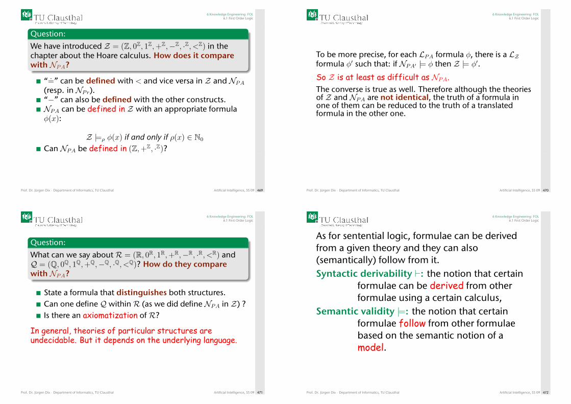
6 Knowledge Engineering: FOL6.1 First Order Logic
Question:
We have introduced Z = (Z, 0Z, 1Z,+Z,−Z, ·Z, <Z) in thechapter about the Hoare calculus. How does it comparewith NPA?
“ .=” can be defined with < and vice versa in Z and NPA(resp. in NPr).“−” can also be defined with the other constructs.NPA can be defined in Z with an appropriate formulaφ(x):
Z |=ρ φ(x) if and only if ρ(x) ∈ N0
Can NPA be defined in (Z,+Z, ·Z)?
Prof. Dr. Jürgen Dix · Department of Informatics, TU Clausthal Artificial Intelligence, SS 09 469
6 Knowledge Engineering: FOL6.1 First Order Logic
To be more precise, for each LPA formula φ, there is a LZformula φ′ such that: if NPA′ |= φ then Z |= φ′.
So Z is at least as difficult as NPA.The converse is true as well. Therefore although the theoriesof Z and NPA are not identical, the truth of a formula inone of them can be reduced to the truth of a translatedformula in the other one.
Prof. Dr. Jürgen Dix · Department of Informatics, TU Clausthal Artificial Intelligence, SS 09 470
6 Knowledge Engineering: FOL6.1 First Order Logic
Question:
What can we say about R = (R, 0R, 1R,+R,−R, ·R, <R) andQ = (Q, 0Q, 1Q,+Q,−Q, ·Q, <Q)? How do they comparewith NPA?
State a formula that distinguishes both structures.Can one define QwithinR (as we did defineNPA in Z) ?Is there an axiomatization of R?
In general, theories of particular structures areundecidable. But it depends on the underlying language.
Prof. Dr. Jürgen Dix · Department of Informatics, TU Clausthal Artificial Intelligence, SS 09 471
6 Knowledge Engineering: FOL6.1 First Order Logic
As for sentential logic, formulae can be derivedfrom a given theory and they can also(semantically) follow from it.Syntactic derivability `: the notion that certain
formulae can be derived from otherformulae using a certain calculus,
Semantic validity |=: the notion that certainformulae follow from other formulaebased on the semantic notion of amodel.
Prof. Dr. Jürgen Dix · Department of Informatics, TU Clausthal Artificial Intelligence, SS 09 472
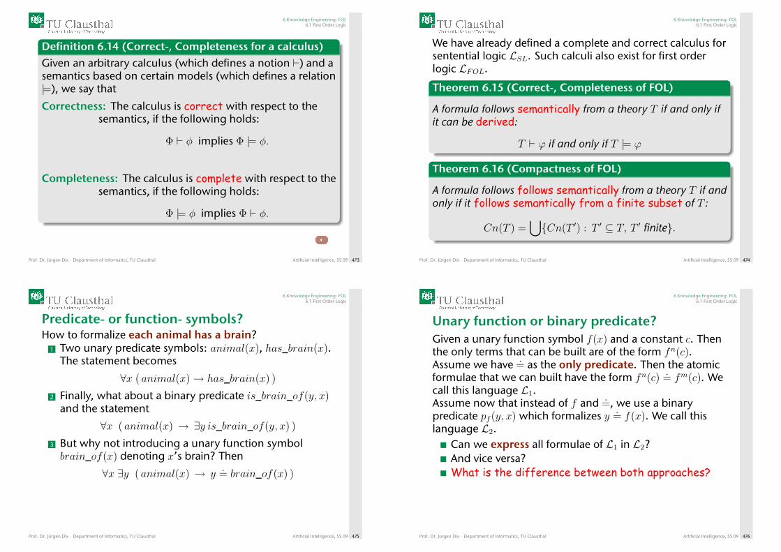
6 Knowledge Engineering: FOL6.1 First Order Logic
Definition 6.14 (Correct-, Completeness for a calculus)Given an arbitrary calculus (which defines a notion `) and asemantics based on certain models (which defines a relation|=), we say that
Correctness: The calculus is correct with respect to thesemantics, if the following holds:
Φ ` φ implies Φ |= φ.
Completeness: The calculus is complete with respect to thesemantics, if the following holds:
Φ |= φ implies Φ ` φ.
Prof. Dr. Jürgen Dix · Department of Informatics, TU Clausthal Artificial Intelligence, SS 09 473
6 Knowledge Engineering: FOL6.1 First Order Logic
We have already defined a complete and correct calculus forsentential logic LSL. Such calculi also exist for first orderlogic LFOL.
Theorem 6.15 (Correct-, Completeness of FOL)
A formula follows semantically from a theory T if and only ifit can be derived:
T ` ϕ if and only if T |= ϕ
Theorem 6.16 (Compactness of FOL)
A formula follows follows semantically from a theory T if andonly if it follows semantically from a finite subset of T :
Cn(T ) =⋃{Cn(T ′) : T ′ ⊆ T, T ′ finite}.
Prof. Dr. Jürgen Dix · Department of Informatics, TU Clausthal Artificial Intelligence, SS 09 474
6 Knowledge Engineering: FOL6.1 First Order Logic
Predicate- or function- symbols?How to formalize each animal has a brain?
1 Two unary predicate symbols: animal(x), has_brain(x).The statement becomes
∀x ( animal(x)→ has_brain(x) )
2 Finally, what about a binary predicate is_brain_of(y, x)and the statement
∀x ( animal(x) → ∃y is_brain_of(y, x) )
3 But why not introducing a unary function symbolbrain_of(x) denoting x’s brain? Then
∀x ∃y ( animal(x) → y.= brain_of(x) )
Prof. Dr. Jürgen Dix · Department of Informatics, TU Clausthal Artificial Intelligence, SS 09 475
6 Knowledge Engineering: FOL6.1 First Order Logic
Unary function or binary predicate?Given a unary function symbol f(x) and a constant c. Thenthe only terms that can be built are of the form fn(c).Assume we have .
= as the only predicate. Then the atomicformulae that we can built have the form fn(c)
.= fm(c). We
call this language L1.Assume now that instead of f and .
=, we use a binarypredicate pf (y, x) which formalizes y .
= f(x). We call thislanguage L2.
Can we express all formulae of L1 in L2?And vice versa?What is the difference between both approaches?
Prof. Dr. Jürgen Dix · Department of Informatics, TU Clausthal Artificial Intelligence, SS 09 476
6 Knowledge Engineering: FOL6.1 First Order Logic
Tuna the catWe formalize again the example of the killed cat,this time in FOL.
1 Jack owns a dog.7→ owns(x, y), dog(x), jack.
2 Dog owners are animal lovers.7→ animal_lover(x).
3 Animal lovers do not kill animals.7→ killer_of(x, y), animal(x).
4 Either Jack or Bill killed Tuna, the cat.7→ bill, tuna, cat(x), killer_of(x, y).
The formalization follows on the blackboard.
Prof. Dr. Jürgen Dix · Department of Informatics, TU Clausthal Artificial Intelligence, SS 09 477
6 Knowledge Engineering: FOL6.2 Sit-Calculus
6.2 Sit-Calculus
Prof. Dr. Jürgen Dix · Department of Informatics, TU Clausthal Artificial Intelligence, SS 09 478
6 Knowledge Engineering: FOL6.2 Sit-Calculus
Question:
How do we axiomatize the Wumpus-world inFOL?
function KB-AGENT( percept) returns an actionstatic: KB, a knowledge base
t, a counter, initially 0, indicating time
TELL(KB, MAKE-PERCEPT-SENTENCE( percept, t))action�ASK(KB, MAKE-ACTION-QUERY(t))TELL(KB, MAKE-ACTION-SENTENCE(action, t))t� t + 1return action
Prof. Dr. Jürgen Dix · Department of Informatics, TU Clausthal Artificial Intelligence, SS 09 479
6 Knowledge Engineering: FOL6.2 Sit-Calculus
Idea:In order to describe actions or their effects consistently weconsider the world as a sequence of situations (snapshots ofthe world). Therefore we have to extend each predicate byan additional argument.
We use the function symbol
result(action, situation)
as the term for the situation which emerges when theaction action is executed in the situation situation.
Actions: Turn_right, Turn_left, Foreward, Shoot, Grab,Release, Climb.
Prof. Dr. Jürgen Dix · Department of Informatics, TU Clausthal Artificial Intelligence, SS 09 480
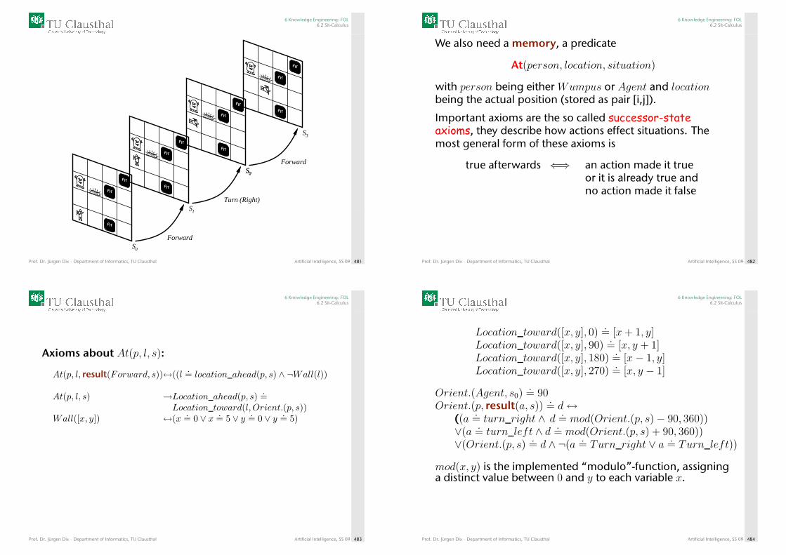
6 Knowledge Engineering: FOL6.2 Sit-Calculus
PIT
PIT
PIT
Gold
PIT
PIT
PIT
Gold
PIT
PIT
PIT
Gold
PIT
PIT
PIT
Gold
Forward
S0
Forward
Turn (Right)S1
S0S2
S3
Prof. Dr. Jürgen Dix · Department of Informatics, TU Clausthal Artificial Intelligence, SS 09 481
6 Knowledge Engineering: FOL6.2 Sit-Calculus
We also need a memory, a predicate
At(person, location, situation)
with person being either Wumpus or Agent and locationbeing the actual position (stored as pair [i,j]).
Important axioms are the so called successor-stateaxioms, they describe how actions effect situations. Themost general form of these axioms is
true afterwards ⇐⇒ an action made it trueor it is already true andno action made it false
Prof. Dr. Jürgen Dix · Department of Informatics, TU Clausthal Artificial Intelligence, SS 09 482
6 Knowledge Engineering: FOL6.2 Sit-Calculus
Axioms about At(p, l, s):
At(p, l, result(Forward, s))↔((l .= location_ahead(p, s) ∧ ¬Wall(l))
At(p, l, s) →Location_ahead(p, s) .=Location_toward(l, Orient.(p, s))
Wall([x, y]) ↔(x .= 0 ∨ x .= 5 ∨ y .= 0 ∨ y .= 5)
Prof. Dr. Jürgen Dix · Department of Informatics, TU Clausthal Artificial Intelligence, SS 09 483
6 Knowledge Engineering: FOL6.2 Sit-Calculus
Location_toward([x, y], 0).= [x+ 1, y]
Location_toward([x, y], 90).= [x, y + 1]
Location_toward([x, y], 180).= [x− 1, y]
Location_toward([x, y], 270).= [x, y − 1]
Orient.(Agent, s0).= 90
Orient.(p, result(a, s)) .= d↔
((a.= turn_right ∧ d
.= mod(Orient.(p, s)− 90, 360))
∨(a.= turn_left ∧ d .
= mod(Orient.(p, s) + 90, 360))∨(Orient.(p, s)
.= d ∧ ¬(a
.= Turn_right ∨ a .
= Turn_left))
mod(x, y) is the implemented “modulo”-function, assigninga distinct value between 0 and y to each variable x.
Prof. Dr. Jürgen Dix · Department of Informatics, TU Clausthal Artificial Intelligence, SS 09 484
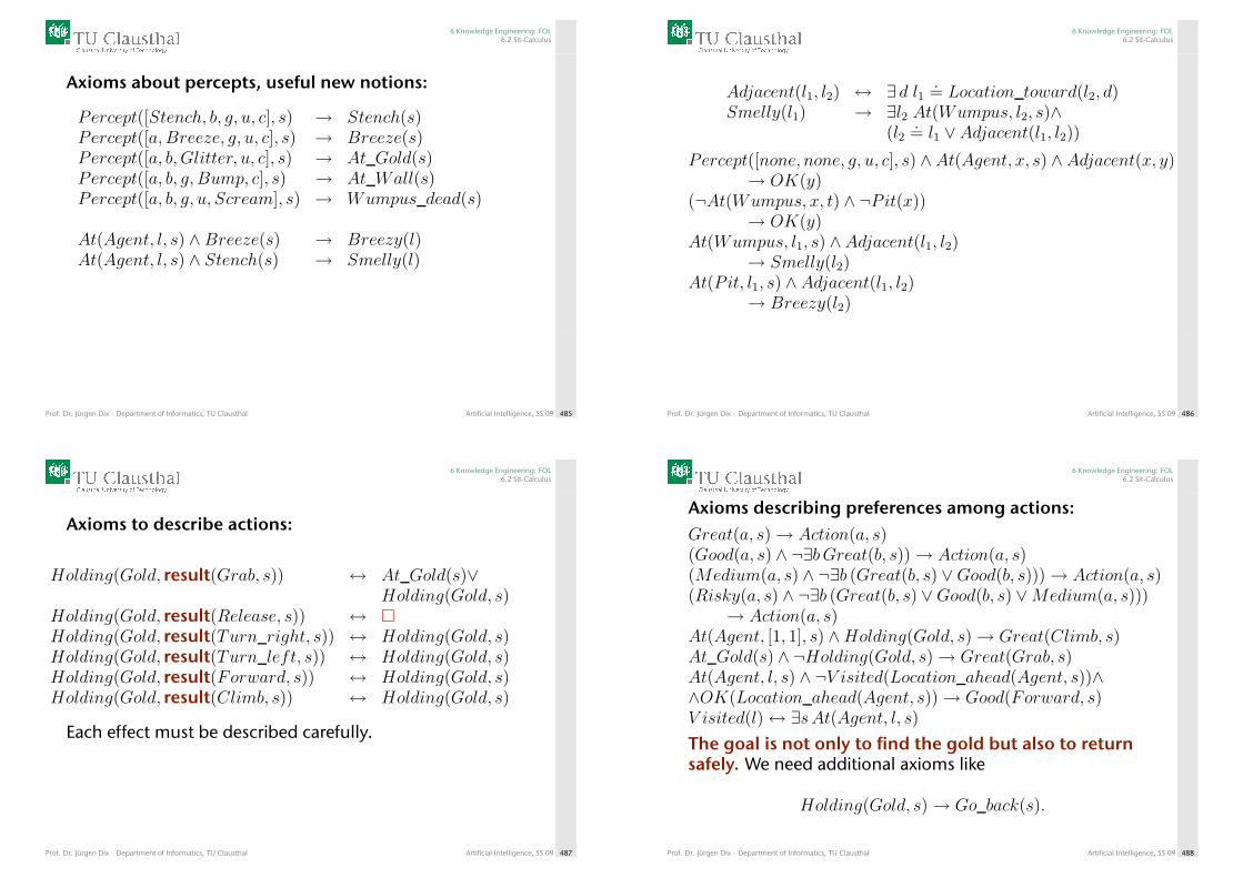
6 Knowledge Engineering: FOL6.2 Sit-Calculus
Axioms about percepts, useful new notions:
Percept([Stench, b, g, u, c], s) → Stench(s)Percept([a,Breeze, g, u, c], s) → Breeze(s)Percept([a, b,Glitter, u, c], s) → At_Gold(s)Percept([a, b, g, Bump, c], s) → At_Wall(s)Percept([a, b, g, u, Scream], s) → Wumpus_dead(s)
At(Agent, l, s) ∧Breeze(s) → Breezy(l)At(Agent, l, s) ∧ Stench(s) → Smelly(l)
Prof. Dr. Jürgen Dix · Department of Informatics, TU Clausthal Artificial Intelligence, SS 09 485
6 Knowledge Engineering: FOL6.2 Sit-Calculus
Adjacent(l1, l2) ↔ ∃ d l1.= Location_toward(l2, d)
Smelly(l1) → ∃l2 At(Wumpus, l2, s)∧(l2
.= l1 ∨ Adjacent(l1, l2))
Percept([none, none, g, u, c], s) ∧ At(Agent, x, s) ∧ Adjacent(x, y)→ OK(y)
(¬At(Wumpus, x, t) ∧ ¬Pit(x))→ OK(y)
At(Wumpus, l1, s) ∧ Adjacent(l1, l2)→ Smelly(l2)
At(Pit, l1, s) ∧ Adjacent(l1, l2)→ Breezy(l2)
Prof. Dr. Jürgen Dix · Department of Informatics, TU Clausthal Artificial Intelligence, SS 09 486
6 Knowledge Engineering: FOL6.2 Sit-Calculus
Axioms to describe actions:
Holding(Gold, result(Grab, s)) ↔ At_Gold(s)∨Holding(Gold, s)
Holding(Gold, result(Release, s)) ↔ �Holding(Gold, result(Turn_right, s)) ↔ Holding(Gold, s)Holding(Gold, result(Turn_left, s)) ↔ Holding(Gold, s)Holding(Gold, result(Forward, s)) ↔ Holding(Gold, s)Holding(Gold, result(Climb, s)) ↔ Holding(Gold, s)
Each effect must be described carefully.
Prof. Dr. Jürgen Dix · Department of Informatics, TU Clausthal Artificial Intelligence, SS 09 487
6 Knowledge Engineering: FOL6.2 Sit-Calculus
Axioms describing preferences among actions:Great(a, s)→ Action(a, s)(Good(a, s) ∧ ¬∃bGreat(b, s))→ Action(a, s)(Medium(a, s) ∧ ¬∃b (Great(b, s) ∨Good(b, s)))→ Action(a, s)(Risky(a, s) ∧ ¬∃b (Great(b, s) ∨Good(b, s) ∨Medium(a, s)))
→ Action(a, s)At(Agent, [1, 1], s) ∧Holding(Gold, s)→ Great(Climb, s)At_Gold(s) ∧ ¬Holding(Gold, s)→ Great(Grab, s)At(Agent, l, s) ∧ ¬V isited(Location_ahead(Agent, s))∧∧OK(Location_ahead(Agent, s))→ Good(Forward, s)V isited(l)↔ ∃sAt(Agent, l, s)The goal is not only to find the gold but also to returnsafely. We need additional axioms like
Holding(Gold, s)→ Go_back(s).
Prof. Dr. Jürgen Dix · Department of Informatics, TU Clausthal Artificial Intelligence, SS 09 488
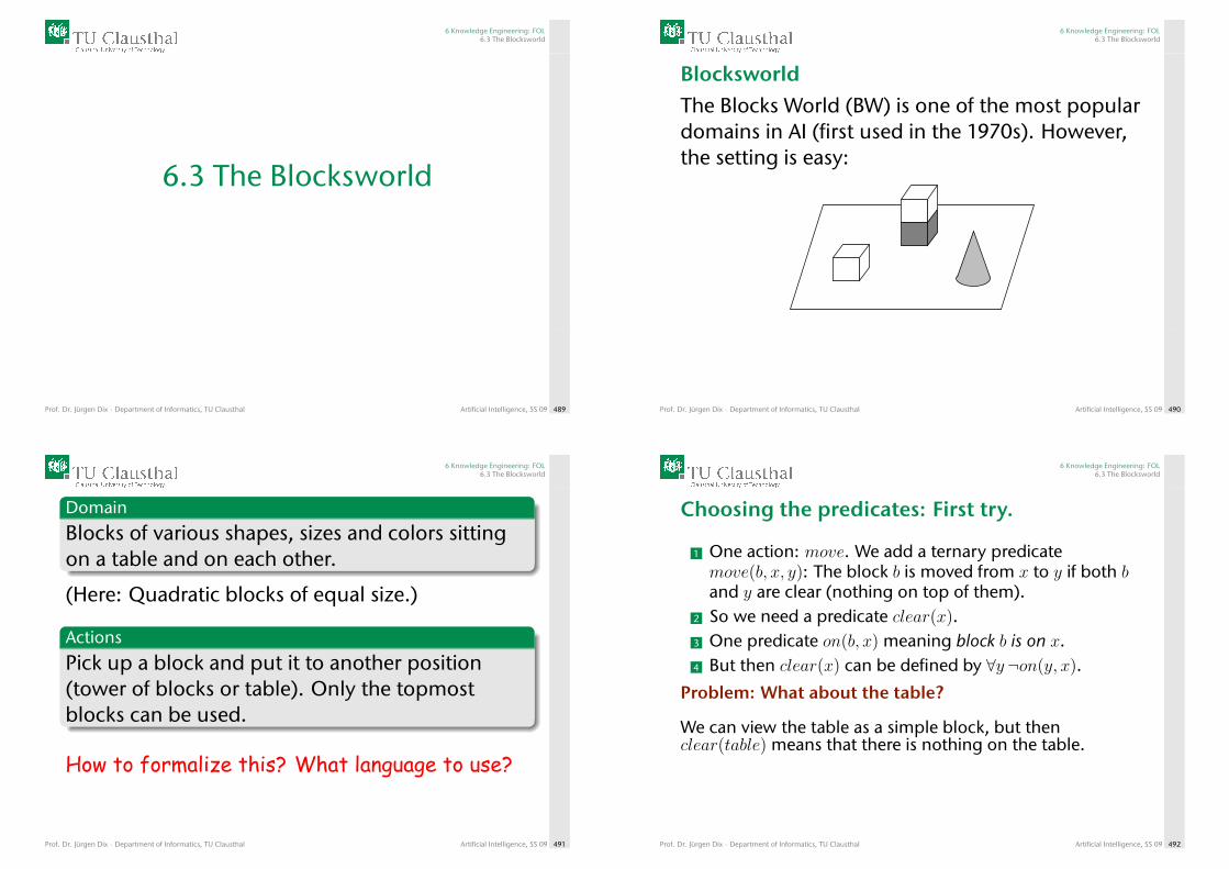
6 Knowledge Engineering: FOL6.3 The Blocksworld
6.3 The Blocksworld
Prof. Dr. Jürgen Dix · Department of Informatics, TU Clausthal Artificial Intelligence, SS 09 489
6 Knowledge Engineering: FOL6.3 The Blocksworld
BlocksworldThe Blocks World (BW) is one of the most populardomains in AI (first used in the 1970s). However,the setting is easy:
Prof. Dr. Jürgen Dix · Department of Informatics, TU Clausthal Artificial Intelligence, SS 09 490
6 Knowledge Engineering: FOL6.3 The Blocksworld
Domain
Blocks of various shapes, sizes and colors sittingon a table and on each other.
(Here: Quadratic blocks of equal size.)
Actions
Pick up a block and put it to another position(tower of blocks or table). Only the topmostblocks can be used.
How to formalize this? What language to use?
Prof. Dr. Jürgen Dix · Department of Informatics, TU Clausthal Artificial Intelligence, SS 09 491
6 Knowledge Engineering: FOL6.3 The Blocksworld
Choosing the predicates: First try.
1 One action: move. We add a ternary predicatemove(b, x, y): The block b is moved from x to y if both band y are clear (nothing on top of them).
2 So we need a predicate clear(x).3 One predicate on(b, x) meaning block b is on x.4 But then clear(x) can be defined by ∀y ¬on(y, x).
Problem: What about the table?
We can view the table as a simple block, but thenclear(table) means that there is nothing on the table.
Prof. Dr. Jürgen Dix · Department of Informatics, TU Clausthal Artificial Intelligence, SS 09 492
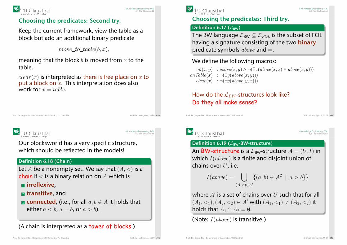
6 Knowledge Engineering: FOL6.3 The Blocksworld
Choosing the predicates: Second try.
Keep the current framework, view the table as ablock but add an additional binary predicate
move_to_table(b, x),
meaning that the block b is moved from x to thetable.
clear(x) is interpreted as there is free place on x toput a block on x. This interpretation does alsowork for x .
= table.
Prof. Dr. Jürgen Dix · Department of Informatics, TU Clausthal Artificial Intelligence, SS 09 493
6 Knowledge Engineering: FOL6.3 The Blocksworld
Choosing the predicates: Third try.Definition 6.17 (LBW)
The BW language LBW ⊆ LFOL is the subset of FOLhaving a signature consisting of the two binarypredicate symbols above and .
=.
We define the following macros:on(x, y) : above(x, y) ∧ ¬(∃z(above(x, z) ∧ above(z, y)))
onTable(x) : ¬(∃y(above(x, y)))clear(x) : ¬(∃y(above(y, x)))
How do the LBW -structures look like?Do they all make sense?
Prof. Dr. Jürgen Dix · Department of Informatics, TU Clausthal Artificial Intelligence, SS 09 494
6 Knowledge Engineering: FOL6.3 The Blocksworld
Our blocksworld has a very specific structure,which should be reflected in the models!
Definition 6.18 (Chain)
Let A be a nonempty set. We say that (A,<) is achain if < is a binary relation on A which is
1 irreflexive,2 transitive, and3 connected, (i.e., for all a, b ∈ A it holds that
either a < b, a = b, or a > b).
(A chain is interpreted as a tower of blocks.)
Prof. Dr. Jürgen Dix · Department of Informatics, TU Clausthal Artificial Intelligence, SS 09 495
6 Knowledge Engineering: FOL6.3 The Blocksworld
Definition 6.19 (LBW-BW-structure)
An BW-structure is a LBW-structure A = (U, I) inwhich I(above) is a finite and disjoint union ofchains over U , i.e.
I(above) =⋃
(A,<)∈A′{(a, b) ∈ A2 | a > b}}
where A′ is a set of chains over U such that for all(A1, <1), (A2, <2) ∈ A′ with (A1, <1) 6= (A2, <2) itholds that A1 ∩ A2 = ∅.
(Note: I(above) is transitive!)
Prof. Dr. Jürgen Dix · Department of Informatics, TU Clausthal Artificial Intelligence, SS 09 496
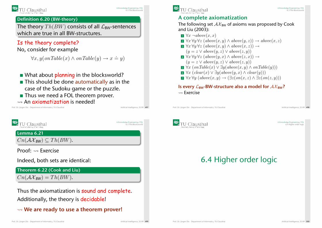
6 Knowledge Engineering: FOL6.3 The Blocksworld
Definition 6.20 (BW-theory)
The theory Th(BW ) consists of all LBW-sentenceswhich are true in all BW-structures.
Is the theory complete?No, consider for example
∀x, y(onTable(x) ∧ onTable(y)→ x.= y)
What about planning in the blocksworld?This should be done automatically as in thecase of the Sudoku game or the puzzle.Thus we need a FOL theorem prover.
An axiomatization is needed!Prof. Dr. Jürgen Dix · Department of Informatics, TU Clausthal Artificial Intelligence, SS 09 497
6 Knowledge Engineering: FOL6.3 The Blocksworld
A complete axiomatizationThe following set AX BW of axioms was proposed by Cookand Liu (2003):
1 ∀x ¬above(x, x)2 ∀x ∀y ∀z (above(x, y) ∧ above(y, z))→ above(x, z)3 ∀x ∀y ∀z (above(x, y) ∧ above(x, z))→
(y = z ∨ above(y, z) ∨ above(z, y))4 ∀x ∀y ∀z (above(y, x) ∧ above(z, x))→
(y = z ∨ above(y, z) ∨ above(z, y))5 ∀x (onTable(x) ∨ ∃y(above(x, y) ∧ onTable(y)))6 ∀x (clear(x) ∨ ∃y(above(y, x) ∧ clear(y)))7 ∀x ∀y (above(x, y)→ (∃z(on(x, z) ∧ ∃z(on(z, y)))
Is every LBW-BW-structure also a model for AX BW? Exercise
Prof. Dr. Jürgen Dix · Department of Informatics, TU Clausthal Artificial Intelligence, SS 09 498
6 Knowledge Engineering: FOL6.3 The Blocksworld
Lemma 6.21
Cn(AX BW) ⊆ Th(BW ).
Proof: Exercise
Indeed, both sets are identical:
Theorem 6.22 (Cook and Liu)
Cn(AX BW) = Th(BW ).
Thus the axiomatization is sound and complete.
Additionally, the theory is decidable!
We are ready to use a theorem prover!
Prof. Dr. Jürgen Dix · Department of Informatics, TU Clausthal Artificial Intelligence, SS 09 499
6 Knowledge Engineering: FOL6.4 Higher order logic
6.4 Higher order logic
Prof. Dr. Jürgen Dix · Department of Informatics, TU Clausthal Artificial Intelligence, SS 09 500
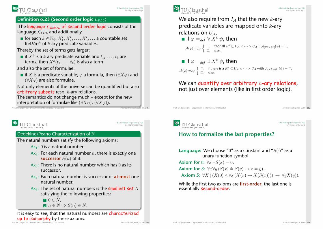
6 Knowledge Engineering: FOL6.4 Higher order logic
Definition 6.23 (Second order logic LPL 2)
The language L2ndOL of second order logic consists of thelanguage LFOL and additionally
for each k ∈ N0: Xk1 , X
k2 , . . . , X
kn, . . . a countable set
RelVark of k-ary predicate variables.Thereby the set of terms gets larger:
if Xk is a k-ary predicate variable and t1, . . . , tk areterms, then Xk(t1, . . . , tk) is also a term
and also the set of formulae:if X is a predicate variable, ϕ a formula, then (∃Xϕ) and(∀Xϕ) are also formulae.
Not only elements of the universe can be quantified but alsoarbitrary subsets resp. k-ary relations.The semantics do not change much – except for the newinterpretation of formulae like (∃Xϕ), (∀Xϕ)).
Prof. Dr. Jürgen Dix · Department of Informatics, TU Clausthal Artificial Intelligence, SS 09 501
6 Knowledge Engineering: FOL6.4 Higher order logic
We also require from IA that the new k-arypredicate variables are mapped onto k-aryrelations on UA.
if ϕ =def ∀Xk ψ, then
A(ϕ) =def
{>, if for all Rk ⊆ UA × · · · × UA : A[Xk/Rk](ψ) = >,�, else.
if ϕ =def ∃Xk ψ, then
A(ϕ) =def
{>, if there is a Rk ⊆ UA × · · · × UA with A[Xk/Rk](ψ) = >,�, else.
We can quantify over arbitrary n-ary relations,not just over elements (like in first order logic).
Prof. Dr. Jürgen Dix · Department of Informatics, TU Clausthal Artificial Intelligence, SS 09 502
6 Knowledge Engineering: FOL6.4 Higher order logic
Dedekind/Peano Characterization of NThe natural numbers satisfy the following axioms:
Ax1: 0 is a natural number.Ax2: For each natural number n, there is exactly one
successor S(n) of it.Ax3: There is no natural number which has 0 as its
successor.Ax4: Each natural number is successor of at most one
natural number.Ax5: The set of natural numbers is the smallest set N
satisfying the following properties:1 0 ∈ N ,2 n ∈ N ⇒ S(n) ∈ N .
It is easy to see, that the natural numbers are characterizedup to isomorphy by these axioms.
Prof. Dr. Jürgen Dix · Department of Informatics, TU Clausthal Artificial Intelligence, SS 09 503
6 Knowledge Engineering: FOL6.4 Higher order logic
How to formalize the last properties?
Language: We choose “0” as a constant and “S(·)” as aunary function symbol.
Axiom for 0: ∀x¬S(x).= 0.
Axiom for S: ∀x∀y (S(x).= S(y)→ x
.= y).
Axiom 5: ∀X ( (X(0) ∧ ∀x (X(x)→ X(S(x)))) → ∀yX(y)).
While the first two axioms are first-order, the last one isessentially second-order.
Prof. Dr. Jürgen Dix · Department of Informatics, TU Clausthal Artificial Intelligence, SS 09 504
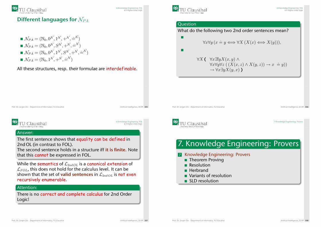
6 Knowledge Engineering: FOL6.4 Higher order logic
Different languages for NPA
NPA = (N0, 0N , 1N ,+N ,
.=N )
NPA = (N0, 0N , SN ,+N ,
.=N )
NPA = (N0, 0N , 1N , SN ,+N ,
.=N )
NPA = (N0, 1N ,+N ,
.=N )
All these structures, resp. their formulae are interdefinable.
Prof. Dr. Jürgen Dix · Department of Informatics, TU Clausthal Artificial Intelligence, SS 09 505
6 Knowledge Engineering: FOL6.4 Higher order logic
QuestionWhat do the following two 2nd order sentences mean?
∀x∀y (x.= y ⇐⇒ ∀X (X(x)⇐⇒ X(y))),
∀X ( ∀x∃!yX(x, y) ∧∀x∀y∀z ( (X(x, z) ∧X(y, z))→ x
.= y))
→ ∀x∃yX(y, x) )
Prof. Dr. Jürgen Dix · Department of Informatics, TU Clausthal Artificial Intelligence, SS 09 506
6 Knowledge Engineering: FOL6.4 Higher order logic
Answer:The first sentence shows that equality can be defined in2nd OL (in contrast to FOL).The second sentence holds in a structure iff it is finite. Notethat this cannot be expressed in FOL.
While the semantics of L2ndOL is a canonical extension ofLFOL, this does not hold for the calculus level. It can beshown that the set of valid sentences in L2ndOL is not evenrecursively enumerable.
Attention:There is no correct and complete calculus for 2nd OrderLogic!
Prof. Dr. Jürgen Dix · Department of Informatics, TU Clausthal Artificial Intelligence, SS 09 507
7 Knowledge Engineering: Provers
7. Knowledge Engineering: Provers7 Knowledge Engineering: Provers
Theorem ProvingResolutionHerbrandVariants of resolutionSLD resolution
Prof. Dr. Jürgen Dix · Department of Informatics, TU Clausthal Artificial Intelligence, SS 09 508
7 Knowledge Engineering: Provers
Content of this chapter:
Provers: We describe several theorem provers that arefreely available and that can handle FOL.
Resolution: There are several calculi for implementing FOL.While the classical ones are not really feasible,resolution calculi can be efficientlyimplemented (and are the basis of mostprovers).
Variants: Resolution implementations often have hugesearch spaces. There are several variants that canbe more efficiently implemented. SLDresolution leads to PROLOG as a programminglanguage.
Prof. Dr. Jürgen Dix · Department of Informatics, TU Clausthal Artificial Intelligence, SS 09 509
7 Knowledge Engineering: Provers7.1 Theorem Proving
7.1 Theorem Proving
Prof. Dr. Jürgen Dix · Department of Informatics, TU Clausthal Artificial Intelligence, SS 09 510
7 Knowledge Engineering: Provers7.1 Theorem Proving
Automated Theorem ProvingDevelopment of computer programs that showthat some statement (the conjecture) is a logicalconsequence of a set of statements (axioms andassumptions).
Prof. Dr. Jürgen Dix · Department of Informatics, TU Clausthal Artificial Intelligence, SS 09 511
7 Knowledge Engineering: Provers7.1 Theorem Proving
Examples
First year math students usually prove thatgroups of order two are commutative.Management consultants might formulateaxioms that describe how organizations growand interact, and from those axioms prove thatorganizational death rates decrease withage.
Prof. Dr. Jürgen Dix · Department of Informatics, TU Clausthal Artificial Intelligence, SS 09 512
7 Knowledge Engineering: Provers7.1 Theorem Proving
Examples (cont.)
Hardware developers might validate thedesign of a circuit by proving a conjecturethat describes a circuit’s performance, givenaxioms that describe the circuit itself.Lazy crosswords fans might prepare a databaseof words and rules of putting a crosswordtogether, and generate the crosswordssolution as a proof.
Prof. Dr. Jürgen Dix · Department of Informatics, TU Clausthal Artificial Intelligence, SS 09 513
7 Knowledge Engineering: Provers7.1 Theorem Proving
The IdeaSpecification of what we have (the system):Assumptions/axioms A1, . . . , An
Specification of what we want: GoalsG1, . . . , Gk
Now, we want to proveor disprove that
A1 ∧ · · · ∧ An |= G1 ∧ · · · ∧Gk
verification!constructive proof synthesis!
Prof. Dr. Jürgen Dix · Department of Informatics, TU Clausthal Artificial Intelligence, SS 09 514
7 Knowledge Engineering: Provers7.1 Theorem Proving
How can we use a theorem prover?Correctness proving: We proveA1 ∧ · · · ∧ An ` G1 ∧ · · · ∧Gk
Testing: We look for counterexamples(models!)Solution synthesis: The constructedproof/model is the solution software synthesis hardware synthesis plan generation etc.
Prof. Dr. Jürgen Dix · Department of Informatics, TU Clausthal Artificial Intelligence, SS 09 515
7 Knowledge Engineering: Provers7.1 Theorem Proving
The language = logic
Often: Classical First Order LogicPossibly: A non-classical logic or higher orderlogic
Prof. Dr. Jürgen Dix · Department of Informatics, TU Clausthal Artificial Intelligence, SS 09 516
7 Knowledge Engineering: Provers7.1 Theorem Proving
The system needs a formal description of theproblem in some logical form.
User prepares the description.Prover attempts to solve the problem.If successful: Proof is the output.If unsuccessful: User can provide guidance,simplify/split the problem, and/or revise thedescription.
This formality is both the underlying strengthand handicap of ATP.
Prof. Dr. Jürgen Dix · Department of Informatics, TU Clausthal Artificial Intelligence, SS 09 517
7 Knowledge Engineering: Provers7.1 Theorem Proving
Pros of logical languages
Allow a precise formal statement of thenecessary information.No ambiguity in the statement of the problem(often the case when using natural language).Force the user to describe the problemprecisely and accurately.The process often leads to a clearer anddeeper understanding of the problemdomain.
Prof. Dr. Jürgen Dix · Department of Informatics, TU Clausthal Artificial Intelligence, SS 09 518
7 Knowledge Engineering: Provers7.1 Theorem Proving
Cons of logical languagesRequire a precise formal statement of thenecessary information many problems are not formalizable!Examples:Creating a good user interface.Creating a system which defends itselfreasonably well against unpredicted situations.
Even for domains which are in principleformalizable: Inaccurate formalizations areeasy to obtain.
Prof. Dr. Jürgen Dix · Department of Informatics, TU Clausthal Artificial Intelligence, SS 09 519
7 Knowledge Engineering: Provers7.1 Theorem Proving
Cons of logical languages (cont.)
Force the user to describe the problemprecisely and accurately. considerable skills needed!Computational intractability.
Prof. Dr. Jürgen Dix · Department of Informatics, TU Clausthal Artificial Intelligence, SS 09 520
7 Knowledge Engineering: Provers7.1 Theorem Proving
Computational complexity of the problem
Propositional logic: co-NP-complete.First-order logic: recursively enumerable(re).Higher-order logic: Not even re.
Prof. Dr. Jürgen Dix · Department of Informatics, TU Clausthal Artificial Intelligence, SS 09 521
7 Knowledge Engineering: Provers7.1 Theorem Proving
Way out of the complexity
Computer-assisted theorem proving
Fully automatictheorem prover
← · · · · · · → Proof checker
Prof. Dr. Jürgen Dix · Department of Informatics, TU Clausthal Artificial Intelligence, SS 09 522
7 Knowledge Engineering: Provers7.1 Theorem Proving
Interactive theorem provers require a humanto give hints to the system.The interaction may be at a very detailed level,where the user guides the inferences made bythe system, or at a much higher level wherethe user determines intermediate lemmas to beproved on the way to the proof of aconjecture.Often: the user defines a number of proofstrategies proving toolbox (e.g., Isabelle).
Prof. Dr. Jürgen Dix · Department of Informatics, TU Clausthal Artificial Intelligence, SS 09 523
7 Knowledge Engineering: Provers7.1 Theorem Proving
Popular ATP techniques
First-order resolution with unification,Higher-order unification,Model elimination,Superposition and term rewriting,Lean theorem proving,Method of analytic tableaux,Mathematical induction,DPLL (Davis-Putnam-Logemann-Loveland algorithm).
All the previously mentioned complexity bounds still apply!
Prof. Dr. Jürgen Dix · Department of Informatics, TU Clausthal Artificial Intelligence, SS 09 524
7 Knowledge Engineering: Provers7.1 Theorem Proving
CASC: CADE ATP System Competition, a yearlycontest of first-order provers for many importantclasses of first-order problems.
http://www.cs.miami.edu/~tptp/CASC/
Prof. Dr. Jürgen Dix · Department of Informatics, TU Clausthal Artificial Intelligence, SS 09 525
7 Knowledge Engineering: Provers7.1 Theorem Proving
Some important first-order provers (all have wonat least one CASC competition division):
EGandalfOtter Prover9/Mace4SETHEOSPASSVampire (won the "world cup for theoremprovers" for eight years: 1999, 2001–2007)Waldmeister (won the CASC UEQ division forthe last ten years: 1997-2006); recentlyembedded in Mathematica
Prof. Dr. Jürgen Dix · Department of Informatics, TU Clausthal Artificial Intelligence, SS 09 526
7 Knowledge Engineering: Provers7.1 Theorem Proving
Other Important Systems
HOLIsabelleMizar
Growing competition: Model checking (especiallyin logics of time, action and knowledge).
Prof. Dr. Jürgen Dix · Department of Informatics, TU Clausthal Artificial Intelligence, SS 09 527
7 Knowledge Engineering: Provers7.1 Theorem Proving
Example: animals, cats, and Garfield
Assumptions:cat(x) -> animal(x).cat(Garfield).
Goals:exists x animal(x).-(exists x animal(x)).
Ontologies, Semantic web
Prof. Dr. Jürgen Dix · Department of Informatics, TU Clausthal Artificial Intelligence, SS 09 528
7 Knowledge Engineering: Provers7.1 Theorem Proving
Prover9 Syntax
Meaning Connective Examplenegation – (–p)disjunction | (p | q | r)conjunction & (p & q & r)implication –> (p –> q)equivalence <–> (p <–> q)universal quant. all (all x all y p(x,y))existential quant. exists (exists x p(x,y))
Prof. Dr. Jürgen Dix · Department of Informatics, TU Clausthal Artificial Intelligence, SS 09 529
7 Knowledge Engineering: Provers7.1 Theorem Proving
Prover9 Syntax (cont.)
Variables start with (lower case) u through zOtherwise: ConstantsFree variables in clauses and formulas areassumed to be universally quantified at theoutermost level
Prover9 uses resolution with refutation. Thus,its inference rules operate on clauses.If non-clausal formulas are input, Prover9immediately translates them to clauses by NNF,Skolemization, and CNF conversions.
Prof. Dr. Jürgen Dix · Department of Informatics, TU Clausthal Artificial Intelligence, SS 09 530
7 Knowledge Engineering: Provers7.1 Theorem Proving
Schubert’s Steamroller
Prof. Dr. Jürgen Dix · Department of Informatics, TU Clausthal Artificial Intelligence, SS 09 531
7 Knowledge Engineering: Provers7.1 Theorem Proving
Success Stories
Fields where ATP has been successfully used:Logic and mathematics.Computer science and engineering (softwarecreation and verification, hardware design andverification – esp. integrated circuit design andverification, and knowledge based systems).Social science.
Prof. Dr. Jürgen Dix · Department of Informatics, TU Clausthal Artificial Intelligence, SS 09 532
7 Knowledge Engineering: Provers7.1 Theorem Proving
Mathematics
EQP: Settling of the Robbins problem (openfor 63 years!)Otter: Several results in quasi-groups;axiomatizations of algebraic structures.Mizar: Cross-verification of the MathematicalLibrary (ongoing).Geometry Expert: New results in Euclideangeometry.NUPRL helped to confirm Higman’s lemmaand Gerard’s paradox.
Prof. Dr. Jürgen Dix · Department of Informatics, TU Clausthal Artificial Intelligence, SS 09 533
7 Knowledge Engineering: Provers7.1 Theorem Proving
Mathematics (cont.)
Results by dedicated provers (no generaltheorem provers):
Proof of four color theorem (verycontroversial: The first mathematical proofwhich was impossible to verify by humans dueto the enormous size of the program’scalculation).
Solving the game of Connect Four.
Prof. Dr. Jürgen Dix · Department of Informatics, TU Clausthal Artificial Intelligence, SS 09 534
7 Knowledge Engineering: Provers7.1 Theorem Proving
Software creation
KIDS: Used to derive scheduling algorithmsthat have outperformed currently usedalgorithms.Amphion (NASA): Determining subroutinesfor satellite guidanceCertifiable Synthesis (NASA).
Prof. Dr. Jürgen Dix · Department of Informatics, TU Clausthal Artificial Intelligence, SS 09 535
7 Knowledge Engineering: Provers7.1 Theorem Proving
Software verification
KIV (Karlsruhe): Verified an implementationof set functions, graph representations andalgorithms, and a Prolog to WAM compiler.PVS: Diagnosis and scheduling algorithms forfault tolerant architectures; requirementsspecification for parts of the space shuttleflight control system.
Prof. Dr. Jürgen Dix · Department of Informatics, TU Clausthal Artificial Intelligence, SS 09 536

7 Knowledge Engineering: Provers7.1 Theorem Proving
Hardware verification
Employed e.g. by IBM, Intel, and Motorola(especially since the Pentium FDIV bug).ACL2: Correctness proof of the floating pointdivide code for AMD5K86 microprocessor.ANALYTICA: Used to verify a division circuitthat implements the floating point standard ofIEEE.RRL: Verification of adder and multipliercircuits.
Prof. Dr. Jürgen Dix · Department of Informatics, TU Clausthal Artificial Intelligence, SS 09 537
7 Knowledge Engineering: Provers7.1 Theorem Proving
Hardware verification (cont.)
PVS: Used to verify a microprocessor foraircraft flight control.Nqthm: Correctness proof of the FM9001microprocessor.HOL: Hardware verification at BellLaboratories.
Prof. Dr. Jürgen Dix · Department of Informatics, TU Clausthal Artificial Intelligence, SS 09 538
7 Knowledge Engineering: Provers7.1 Theorem Proving
Verification of critical section
Prof. Dr. Jürgen Dix · Department of Informatics, TU Clausthal Artificial Intelligence, SS 09 539
7 Knowledge Engineering: Provers7.2 Resolution
7.2 Resolution
Prof. Dr. Jürgen Dix · Department of Informatics, TU Clausthal Artificial Intelligence, SS 09 540
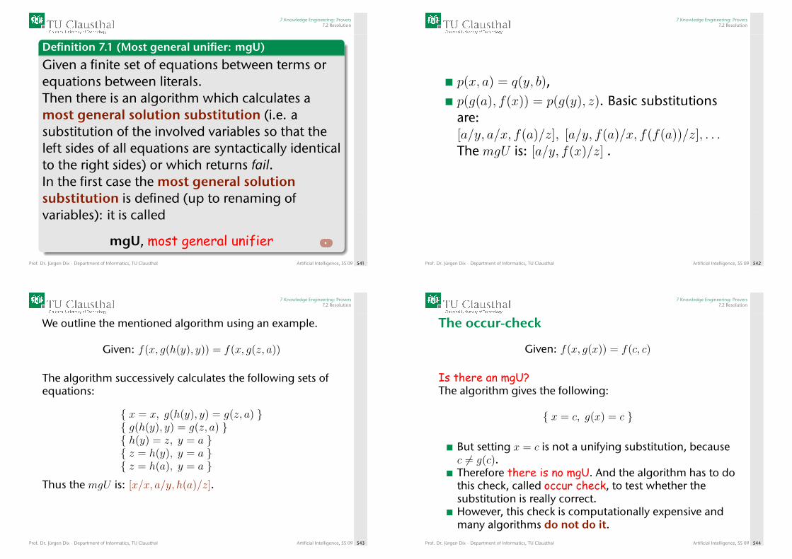
7 Knowledge Engineering: Provers7.2 Resolution
Definition 7.1 (Most general unifier: mgU)
Given a finite set of equations between terms orequations between literals.Then there is an algorithm which calculates amost general solution substitution (i.e. asubstitution of the involved variables so that theleft sides of all equations are syntactically identicalto the right sides) or which returns fail.In the first case the most general solutionsubstitution is defined (up to renaming ofvariables): it is called
mgU, most general unifierProf. Dr. Jürgen Dix · Department of Informatics, TU Clausthal Artificial Intelligence, SS 09 541
7 Knowledge Engineering: Provers7.2 Resolution
p(x, a) = q(y, b),p(g(a), f(x)) = p(g(y), z). Basic substitutionsare:[a/y, a/x, f(a)/z], [a/y, f(a)/x, f(f(a))/z], . . .The mgU is: [a/y, f(x)/z] .
Prof. Dr. Jürgen Dix · Department of Informatics, TU Clausthal Artificial Intelligence, SS 09 542
7 Knowledge Engineering: Provers7.2 Resolution
We outline the mentioned algorithm using an example.
Given: f(x, g(h(y), y)) = f(x, g(z, a))
The algorithm successively calculates the following sets ofequations:
{ x = x, g(h(y), y) = g(z, a) }{ g(h(y), y) = g(z, a) }{ h(y) = z, y = a }{ z = h(y), y = a }{ z = h(a), y = a }
Thus the mgU is: [x/x, a/y, h(a)/z].
Prof. Dr. Jürgen Dix · Department of Informatics, TU Clausthal Artificial Intelligence, SS 09 543
7 Knowledge Engineering: Provers7.2 Resolution
The occur-check
Given: f(x, g(x)) = f(c, c)
Is there an mgU?The algorithm gives the following:
{ x = c, g(x) = c }
But setting x = c is not a unifying substitution, becausec 6= g(c).Therefore there is no mgU. And the algorithm has to dothis check, called occur check, to test whether thesubstitution is really correct.However, this check is computationally expensive andmany algorithms do not do it.
Prof. Dr. Jürgen Dix · Department of Informatics, TU Clausthal Artificial Intelligence, SS 09 544
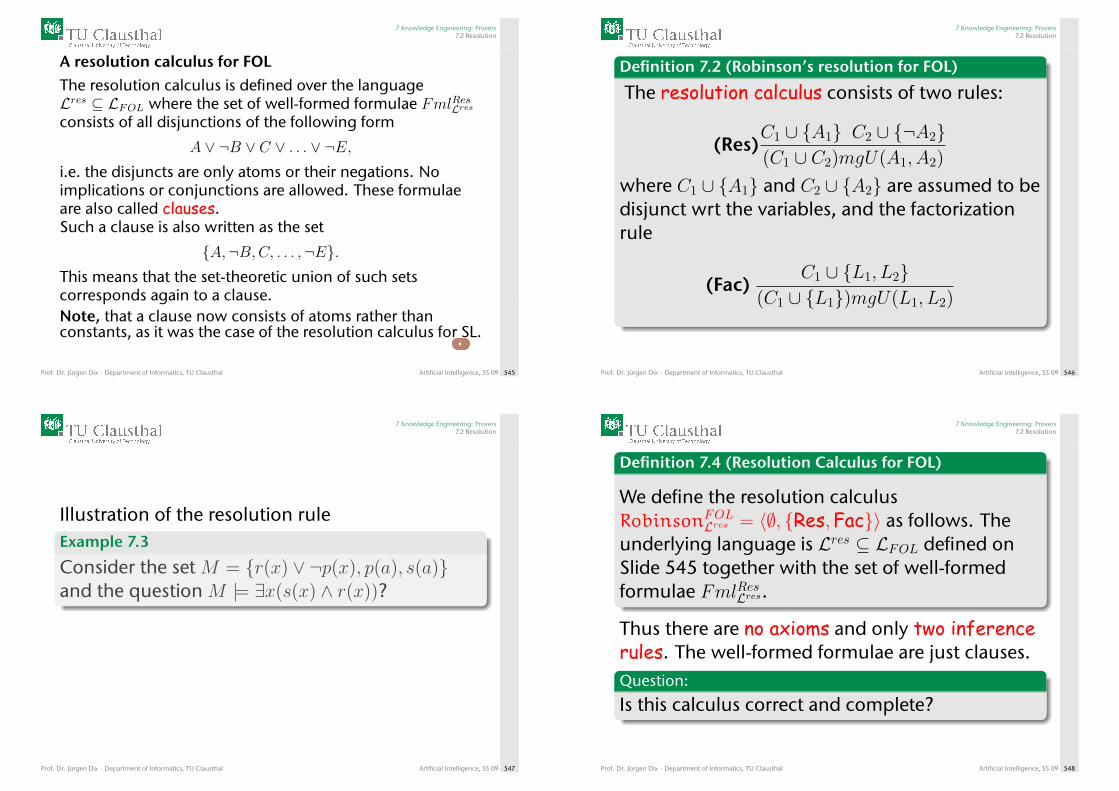
7 Knowledge Engineering: Provers7.2 Resolution
A resolution calculus for FOLThe resolution calculus is defined over the languageLres ⊆ LFOL where the set of well-formed formulae FmlResLresconsists of all disjunctions of the following form
A ∨ ¬B ∨ C ∨ . . . ∨ ¬E,i.e. the disjuncts are only atoms or their negations. Noimplications or conjunctions are allowed. These formulaeare also called clauses.Such a clause is also written as the set
{A,¬B,C, . . . ,¬E}.This means that the set-theoretic union of such setscorresponds again to a clause.Note, that a clause now consists of atoms rather thanconstants, as it was the case of the resolution calculus for SL.
Prof. Dr. Jürgen Dix · Department of Informatics, TU Clausthal Artificial Intelligence, SS 09 545
7 Knowledge Engineering: Provers7.2 Resolution
Definition 7.2 (Robinson’s resolution for FOL)
The resolution calculus consists of two rules:
(Res)C1 ∪ {A1} C2 ∪ {¬A2}(C1 ∪ C2)mgU(A1, A2)
where C1 ∪ {A1} and C2 ∪ {A2} are assumed to bedisjunct wrt the variables, and the factorizationrule
(Fac)C1 ∪ {L1, L2}
(C1 ∪ {L1})mgU(L1, L2)
Prof. Dr. Jürgen Dix · Department of Informatics, TU Clausthal Artificial Intelligence, SS 09 546
7 Knowledge Engineering: Provers7.2 Resolution
Illustration of the resolution ruleExample 7.3
Consider the set M = {r(x) ∨ ¬p(x), p(a), s(a)}and the question M |= ∃x(s(x) ∧ r(x))?
Prof. Dr. Jürgen Dix · Department of Informatics, TU Clausthal Artificial Intelligence, SS 09 547
7 Knowledge Engineering: Provers7.2 Resolution
Definition 7.4 (Resolution Calculus for FOL)
We define the resolution calculusRobinsonFOL
Lres = 〈∅, {Res,Fac}〉 as follows. Theunderlying language is Lres ⊆ LFOL defined onSlide 545 together with the set of well-formedformulae FmlResLres.
Thus there are no axioms and only two inferencerules. The well-formed formulae are just clauses.Question:
Is this calculus correct and complete?
Prof. Dr. Jürgen Dix · Department of Informatics, TU Clausthal Artificial Intelligence, SS 09 548

7 Knowledge Engineering: Provers7.2 Resolution
Question:
Why do we need factorization?
Answer:Consider
M = {{s(x1), s(x2)}, {¬s(y1),¬s(y2)}}
Resolving both clauses gives
{s(x1)} ∪ {¬s(y1)}
or variants of it.Resolving this new clause with one in M only leads tovariants of the respective clause in M .
Prof. Dr. Jürgen Dix · Department of Informatics, TU Clausthal Artificial Intelligence, SS 09 549
7 Knowledge Engineering: Provers7.2 Resolution
Answer (continued):
� can not be derived (using resolution only).
Factorization solves the problem, we can deduceboth s(x) and ¬s(y), and from there the emptyclause.
Theorem 7.5 (Resolution is refutation complete)
Robinsons resolution calculus RobinsonFOLLres is
refutation complete: Given an unsatisfiable set,the empty clause can eventually be derived usingresolution and factorization.
Prof. Dr. Jürgen Dix · Department of Informatics, TU Clausthal Artificial Intelligence, SS 09 550
7 Knowledge Engineering: Provers7.2 Resolution
What to do if the formulae are not clauses?
In that case, we have to transform them intoclauses of the required form.
Let us considerExample 7.6
LetM = {∃x∃y Q(x) ∧ ¬Q(y), ∀x∃y P (x, y)→ ¬Q(y)}.How to deal with the existential quantifiers?
Prof. Dr. Jürgen Dix · Department of Informatics, TU Clausthal Artificial Intelligence, SS 09 551
7 Knowledge Engineering: Provers7.2 Resolution
The first formula is easy to transform: we just addtwo new constants c, c′ and instantiate them forthe variables. This leads to Q(c) ∧ ¬Q(c′), or thetwo clauses Q(c) and Q(c′).
The second formula is more complicated, becausethere is no single y. We have to take into account,that the y usually depends on the chosen x.Therefore we introduce a function symbol f(x):∀xP (x, f(x))→ ¬Q(f(x)). Then we have totransform the formula into disjunctive form:∀x¬P (x, f(x)) ∨ ¬Q(f(x)).
Prof. Dr. Jürgen Dix · Department of Informatics, TU Clausthal Artificial Intelligence, SS 09 552
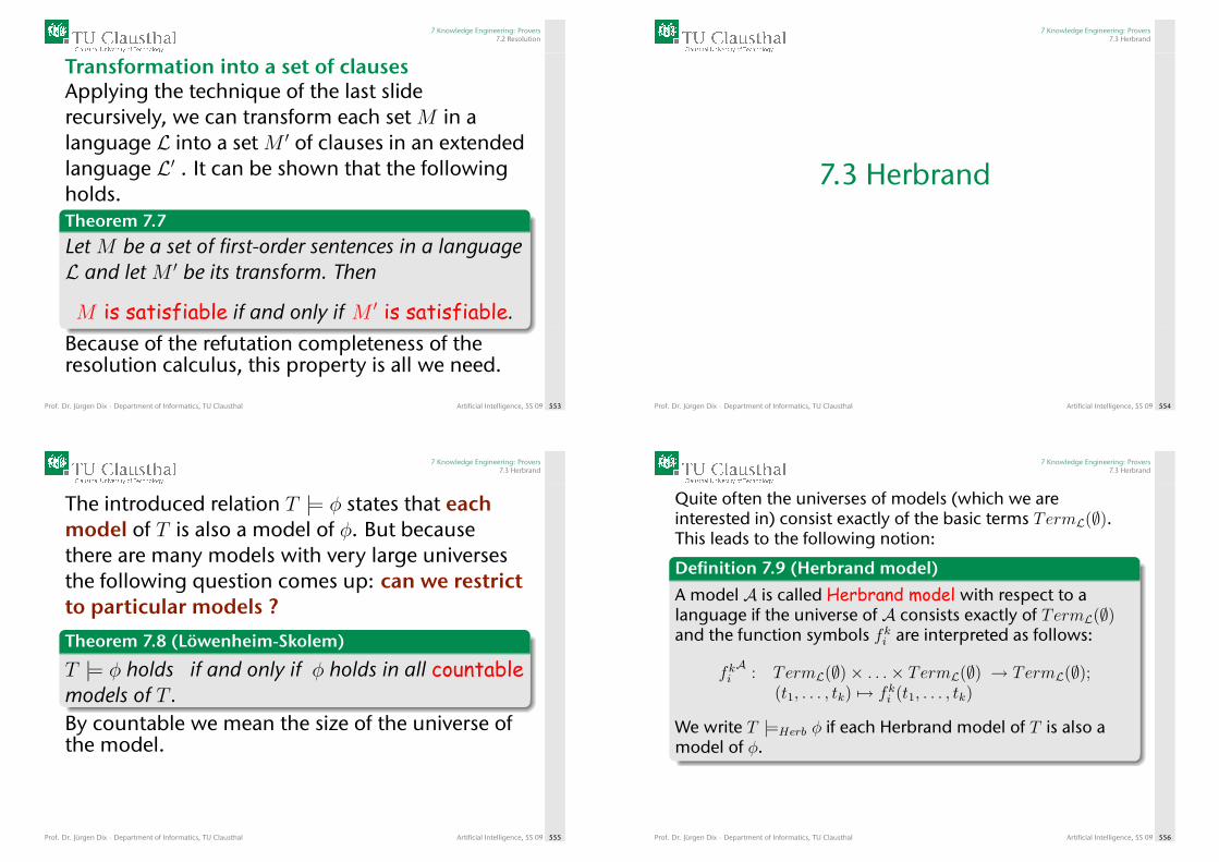
7 Knowledge Engineering: Provers7.2 Resolution
Transformation into a set of clausesApplying the technique of the last sliderecursively, we can transform each set M in alanguage L into a set M ′ of clauses in an extendedlanguage L′ . It can be shown that the followingholds.Theorem 7.7
Let M be a set of first-order sentences in a languageL and let M ′ be its transform. Then
M is satisfiable if and only if M ′ is satisfiable.
Because of the refutation completeness of theresolution calculus, this property is all we need.
Prof. Dr. Jürgen Dix · Department of Informatics, TU Clausthal Artificial Intelligence, SS 09 553
7 Knowledge Engineering: Provers7.3 Herbrand
7.3 Herbrand
Prof. Dr. Jürgen Dix · Department of Informatics, TU Clausthal Artificial Intelligence, SS 09 554
7 Knowledge Engineering: Provers7.3 Herbrand
The introduced relation T |= φ states that eachmodel of T is also a model of φ. But becausethere are many models with very large universesthe following question comes up: can we restrictto particular models ?
Theorem 7.8 (Löwenheim-Skolem)
T |= φ holds if and only if φ holds in all countablemodels of T .By countable we mean the size of the universe ofthe model.
Prof. Dr. Jürgen Dix · Department of Informatics, TU Clausthal Artificial Intelligence, SS 09 555
7 Knowledge Engineering: Provers7.3 Herbrand
Quite often the universes of models (which we areinterested in) consist exactly of the basic terms TermL(∅).This leads to the following notion:
Definition 7.9 (Herbrand model)
A model A is called Herbrand model with respect to alanguage if the universe of A consists exactly of TermL(∅)and the function symbols fki are interpreted as follows:
fkiA
: TermL(∅)× . . .× TermL(∅) → TermL(∅);(t1, . . . , tk) 7→ fki (t1, . . . , tk)
We write T |=Herb φ if each Herbrand model of T is also amodel of φ.
Prof. Dr. Jürgen Dix · Department of Informatics, TU Clausthal Artificial Intelligence, SS 09 556
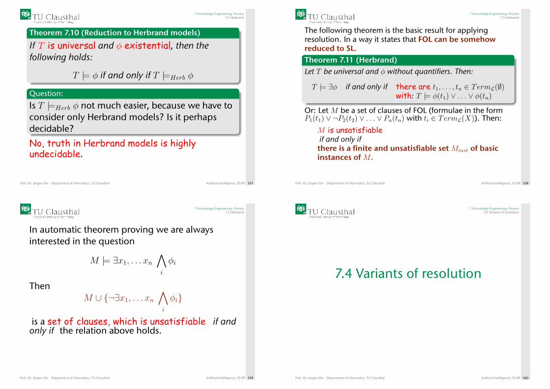
7 Knowledge Engineering: Provers7.3 Herbrand
Theorem 7.10 (Reduction to Herbrand models)
If T is universal and φ existential, then thefollowing holds:
T |= φ if and only if T |=Herb φ
Question:
Is T |=Herb φ not much easier, because we have toconsider only Herbrand models? Is it perhapsdecidable?
No, truth in Herbrand models is highlyundecidable.
Prof. Dr. Jürgen Dix · Department of Informatics, TU Clausthal Artificial Intelligence, SS 09 557
7 Knowledge Engineering: Provers7.3 Herbrand
The following theorem is the basic result for applyingresolution. In a way it states that FOL can be somehowreduced to SL.Theorem 7.11 (Herbrand)Let T be universal and φ without quantifiers. Then:
T |= ∃φ if and only if there are t1, . . . , tn ∈ TermL(∅)with: T |= φ(t1) ∨ . . . ∨ φ(tn)
Or: Let M be a set of clauses of FOL (formulae in the formP1(t1) ∨ ¬P2(t2) ∨ . . . ∨ Pn(tn) with ti ∈ TermL(X)). Then:
M is unsatisfiableif and only ifthere is a finite and unsatisfiable set Minst of basicinstances of M .
Prof. Dr. Jürgen Dix · Department of Informatics, TU Clausthal Artificial Intelligence, SS 09 558
7 Knowledge Engineering: Provers7.3 Herbrand
In automatic theorem proving we are alwaysinterested in the question
M |= ∃x1, . . . xn∧i
φi
ThenM ∪ {¬∃x1, . . . xn
∧i
φi}
is a set of clauses, which is unsatisfiable if andonly if the relation above holds.
Prof. Dr. Jürgen Dix · Department of Informatics, TU Clausthal Artificial Intelligence, SS 09 559
7 Knowledge Engineering: Provers7.4 Variants of resolution
7.4 Variants of resolution
Prof. Dr. Jürgen Dix · Department of Informatics, TU Clausthal Artificial Intelligence, SS 09 560
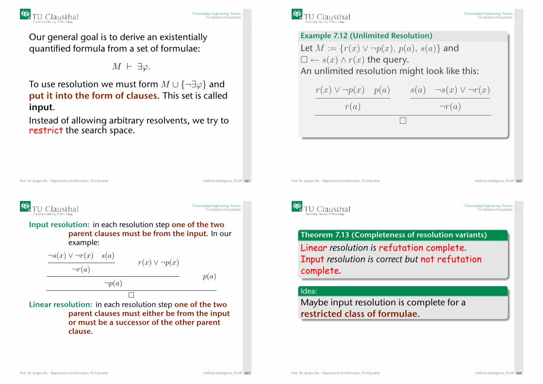
7 Knowledge Engineering: Provers7.4 Variants of resolution
Our general goal is to derive an existentiallyquantified formula from a set of formulae:
M ` ∃ϕ.
To use resolution we must form M ∪ {¬∃ϕ} andput it into the form of clauses. This set is calledinput.Instead of allowing arbitrary resolvents, we try torestrict the search space.
Prof. Dr. Jürgen Dix · Department of Informatics, TU Clausthal Artificial Intelligence, SS 09 561
7 Knowledge Engineering: Provers7.4 Variants of resolution
Example 7.12 (Unlimited Resolution)
Let M := {r(x) ∨ ¬p(x), p(a), s(a)} and�← s(x) ∧ r(x) the query.An unlimited resolution might look like this:
r(x) ∨ ¬p(x) p(a)
r(a)
s(a) ¬s(x) ∨ ¬r(x)
¬r(a)
�
Prof. Dr. Jürgen Dix · Department of Informatics, TU Clausthal Artificial Intelligence, SS 09 562
7 Knowledge Engineering: Provers7.4 Variants of resolution
Input resolution: in each resolution step one of the twoparent clauses must be from the input. In ourexample:
¬s(x) ∨ ¬r(x) s(a)
¬r(a)r(x) ∨ ¬p(x)
¬p(a)p(a)
�Linear resolution: in each resolution step one of the two
parent clauses must either be from the inputor must be a successor of the other parentclause.
Prof. Dr. Jürgen Dix · Department of Informatics, TU Clausthal Artificial Intelligence, SS 09 563
7 Knowledge Engineering: Provers7.4 Variants of resolution
Theorem 7.13 (Completeness of resolution variants)
Linear resolution is refutation complete.Input resolution is correct but not refutationcomplete.
Idea:
Maybe input resolution is complete for arestricted class of formulae.
Prof. Dr. Jürgen Dix · Department of Informatics, TU Clausthal Artificial Intelligence, SS 09 564
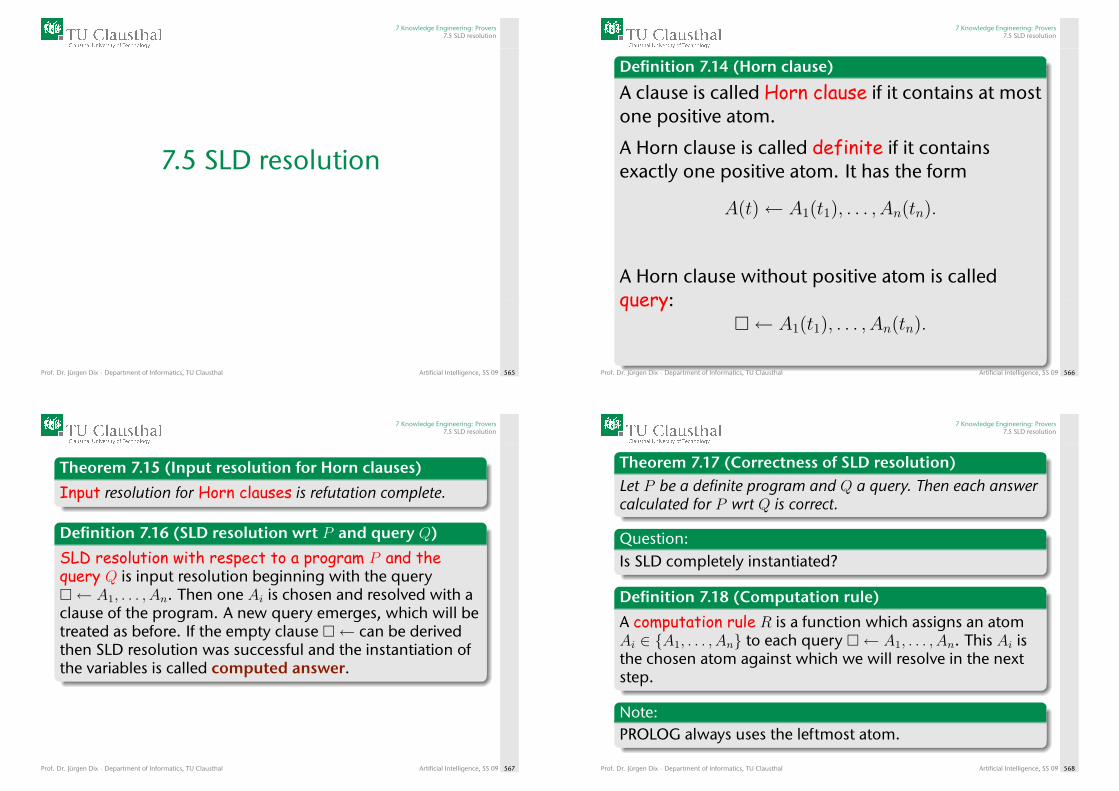
7 Knowledge Engineering: Provers7.5 SLD resolution
7.5 SLD resolution
Prof. Dr. Jürgen Dix · Department of Informatics, TU Clausthal Artificial Intelligence, SS 09 565
7 Knowledge Engineering: Provers7.5 SLD resolution
Definition 7.14 (Horn clause)
A clause is called Horn clause if it contains at mostone positive atom.
A Horn clause is called definite if it containsexactly one positive atom. It has the form
A(t)← A1(t1), . . . , An(tn).
A Horn clause without positive atom is calledquery:
�← A1(t1), . . . , An(tn).
Prof. Dr. Jürgen Dix · Department of Informatics, TU Clausthal Artificial Intelligence, SS 09 566
7 Knowledge Engineering: Provers7.5 SLD resolution
Theorem 7.15 (Input resolution for Horn clauses)
Input resolution for Horn clauses is refutation complete.
Definition 7.16 (SLD resolution wrt P and query Q)
SLD resolution with respect to a program P and thequery Q is input resolution beginning with the query�← A1, . . . , An. Then one Ai is chosen and resolved with aclause of the program. A new query emerges, which will betreated as before. If the empty clause �← can be derivedthen SLD resolution was successful and the instantiation ofthe variables is called computed answer.
Prof. Dr. Jürgen Dix · Department of Informatics, TU Clausthal Artificial Intelligence, SS 09 567
7 Knowledge Engineering: Provers7.5 SLD resolution
Theorem 7.17 (Correctness of SLD resolution)Let P be a definite program and Q a query. Then each answercalculated for P wrt Q is correct.
Question:Is SLD completely instantiated?
Definition 7.18 (Computation rule)
A computation rule R is a function which assigns an atomAi ∈ {A1, . . . , An} to each query �← A1, . . . , An. This Ai isthe chosen atom against which we will resolve in the nextstep.
Note:PROLOG always uses the leftmost atom.
Prof. Dr. Jürgen Dix · Department of Informatics, TU Clausthal Artificial Intelligence, SS 09 568
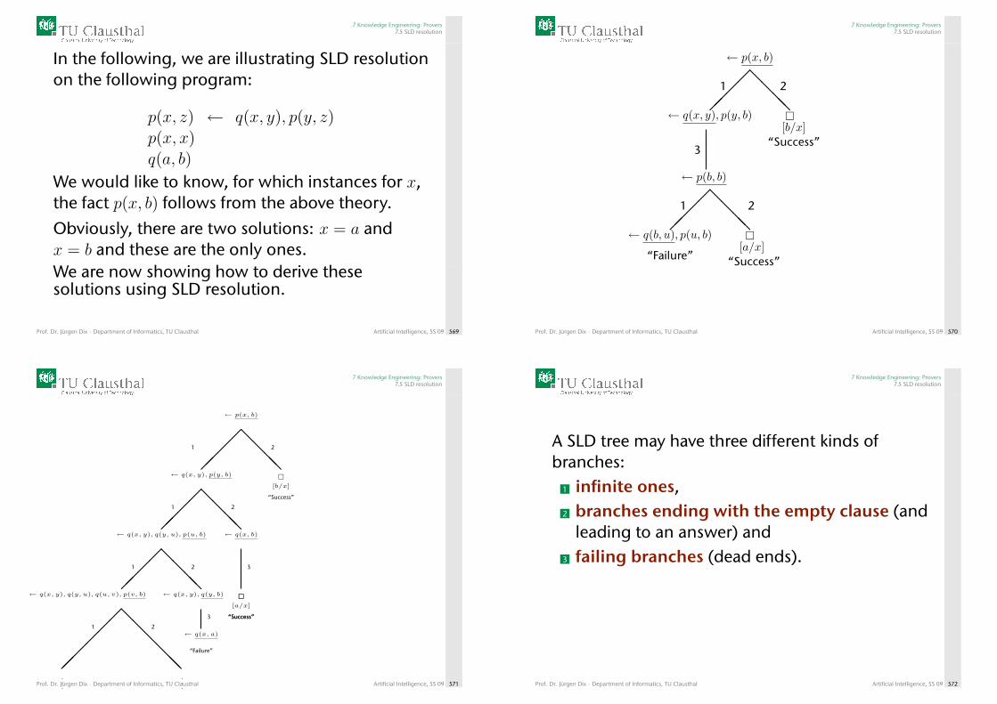
7 Knowledge Engineering: Provers7.5 SLD resolution
In the following, we are illustrating SLD resolutionon the following program:
p(x, z) ← q(x, y), p(y, z)p(x, x)q(a, b)
We would like to know, for which instances for x,the fact p(x, b) follows from the above theory.
Obviously, there are two solutions: x = a andx = b and these are the only ones.We are now showing how to derive thesesolutions using SLD resolution.
Prof. Dr. Jürgen Dix · Department of Informatics, TU Clausthal Artificial Intelligence, SS 09 569
7 Knowledge Engineering: Provers7.5 SLD resolution
← p(x, b)
← q(x, y), p(y, b)
← p(b, b)
← q(b, u), p(u, b)
�[b/x]
“Success”
“Failure”
�
“Success”[a/x]
����
��
��
@@@@
@@@@
1
1
2
2
3
Prof. Dr. Jürgen Dix · Department of Informatics, TU Clausthal Artificial Intelligence, SS 09 570
7 Knowledge Engineering: Provers7.5 SLD resolution
← p(x, b)
← q(x, y), p(y, b)
← q(x, y), q(y, u), p(u, b) ← q(x, b)
← q(x, y), q(y, u), q(u, v), p(v, b) ← q(x, y), q(y, b)
← q(x, a)
�
[b/x]
“Success”
“Failure”
�
“Success”
�
“Success”
[a/x]
����
��
��
��
��
��
��
��
@@@@
@@@@
@@@@
@@@@@@
.
.
.
.
.
.
1
1
1
1
2
2
2
2
3
3
Prof. Dr. Jürgen Dix · Department of Informatics, TU Clausthal Artificial Intelligence, SS 09 571
7 Knowledge Engineering: Provers7.5 SLD resolution
A SLD tree may have three different kinds ofbranches:
1 infinite ones,2 branches ending with the empty clause (and
leading to an answer) and3 failing branches (dead ends).
Prof. Dr. Jürgen Dix · Department of Informatics, TU Clausthal Artificial Intelligence, SS 09 572
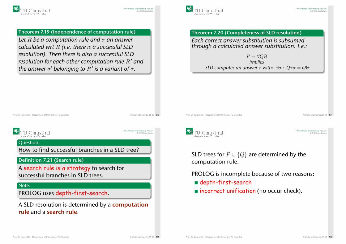
7 Knowledge Engineering: Provers7.5 SLD resolution
Theorem 7.19 (Independence of computation rule)
Let R be a computation rule and σ an answercalculated wrt R (i.e. there is a successful SLDresolution). Then there is also a successful SLDresolution for each other computation rule R’ andthe answer σ′ belonging to R’ is a variant of σ.
Prof. Dr. Jürgen Dix · Department of Informatics, TU Clausthal Artificial Intelligence, SS 09 573
7 Knowledge Engineering: Provers7.5 SLD resolution
Theorem 7.20 (Completeness of SLD resolution)
Each correct answer substitution is subsumedthrough a calculated answer substitution. I.e.:
P |= ∀QΘimplies
SLD computes an answer τ with: ∃σ : Qτσ = QΘ
Prof. Dr. Jürgen Dix · Department of Informatics, TU Clausthal Artificial Intelligence, SS 09 574
7 Knowledge Engineering: Provers7.5 SLD resolution
Question:
How to find successful branches in a SLD tree?
Definition 7.21 (Search rule)
A search rule is a strategy to search forsuccessful branches in SLD trees.
Note:
PROLOG uses depth-first-search.
A SLD resolution is determined by a computationrule and a search rule.
Prof. Dr. Jürgen Dix · Department of Informatics, TU Clausthal Artificial Intelligence, SS 09 575
7 Knowledge Engineering: Provers7.5 SLD resolution
SLD trees for P ∪ {Q} are determined by thecomputation rule.
PROLOG is incomplete because of two reasons:depth-first-searchincorrect unification (no occur check).
Prof. Dr. Jürgen Dix · Department of Informatics, TU Clausthal Artificial Intelligence, SS 09 576
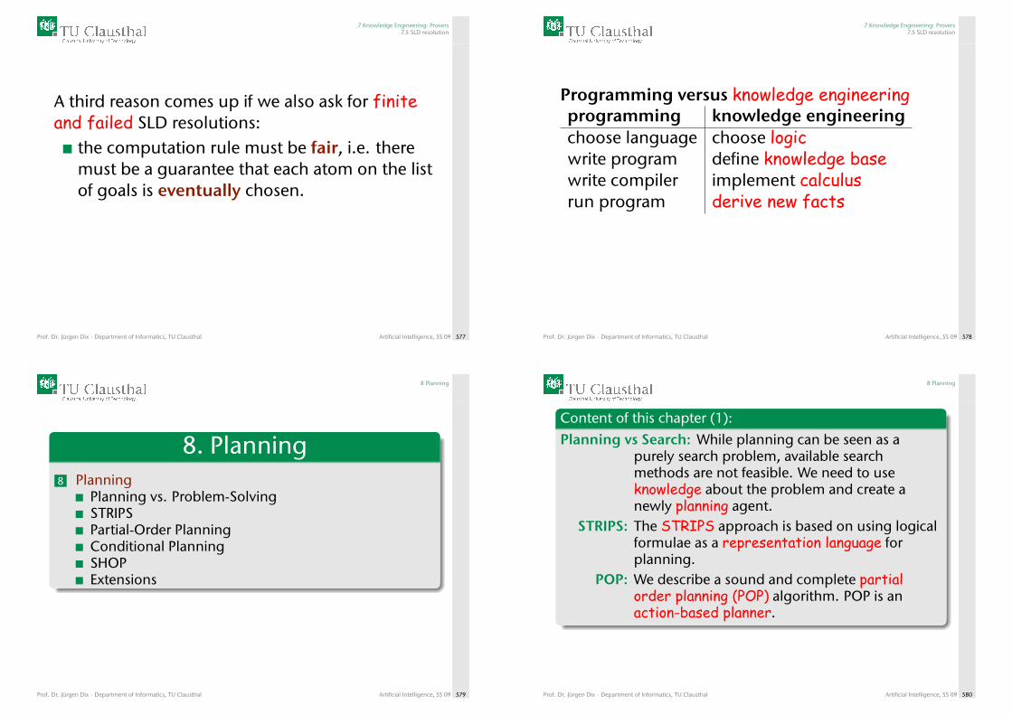
7 Knowledge Engineering: Provers7.5 SLD resolution
A third reason comes up if we also ask for finiteand failed SLD resolutions:
the computation rule must be fair, i.e. theremust be a guarantee that each atom on the listof goals is eventually chosen.
Prof. Dr. Jürgen Dix · Department of Informatics, TU Clausthal Artificial Intelligence, SS 09 577
7 Knowledge Engineering: Provers7.5 SLD resolution
Programming versus knowledge engineeringprogramming knowledge engineeringchoose language choose logicwrite program define knowledge basewrite compiler implement calculusrun program derive new facts
Prof. Dr. Jürgen Dix · Department of Informatics, TU Clausthal Artificial Intelligence, SS 09 578
8 Planning
8. Planning8 Planning
Planning vs. Problem-SolvingSTRIPSPartial-Order PlanningConditional PlanningSHOPExtensions
Prof. Dr. Jürgen Dix · Department of Informatics, TU Clausthal Artificial Intelligence, SS 09 579
8 Planning
Content of this chapter (1):
Planning vs Search: While planning can be seen as apurely search problem, available searchmethods are not feasible. We need to useknowledge about the problem and create anewly planning agent.
STRIPS: The STRIPS approach is based on using logicalformulae as a representation language forplanning.
POP: We describe a sound and complete partialorder planning (POP) algorithm. POP is anaction-based planner.
Prof. Dr. Jürgen Dix · Department of Informatics, TU Clausthal Artificial Intelligence, SS 09 580

8 Planning
Content of this chapter (2):
Conditional Planning: Often a plan cannot be completelyconstructed a priori, because the environment isdynamic. The we need sensing actions thathave to be checked at run-time.
SHOP: We introduce HTN-planning, which is based onHierarchical Task networks. HTN planners usedomain knowledge and are more expressivethan action-based planners. SHOP is one of themost efficient HTN planners.
Extensions: We briefly describe replanning and how tocombine it with conditional planning.
Prof. Dr. Jürgen Dix · Department of Informatics, TU Clausthal Artificial Intelligence, SS 09 581
8 Planning8.1 Planning vs. Problem-Solving
8.1 Planning vs. Problem-Solving
Prof. Dr. Jürgen Dix · Department of Informatics, TU Clausthal Artificial Intelligence, SS 09 582
8 Planning8.1 Planning vs. Problem-Solving
Motivation:
problem-solving agent: The effects of a staticsequence of actions are determined.
knowledge-based agent: Actions can be chosen.
We try to merge both into a planning agent.
Prof. Dr. Jürgen Dix · Department of Informatics, TU Clausthal Artificial Intelligence, SS 09 583
8 Planning8.1 Planning vs. Problem-Solving
function SIMPLE-PLANNING-AGENT( percept) returns an actionstatic: KB, a knowledge base (includes action descriptions)
p, a plan, initially NoPlant, a counter, initially 0, indicating time
local variables: G, a goalcurrent, a current state description
TELL(KB, MAKE-PERCEPT-SENTENCE( percept, t))current� STATE-DESCRIPTION(KB, t)if p = NoPlan then
G�ASK(KB, MAKE-GOAL-QUERY(t))p� IDEAL-PLANNER(current, G, KB)
if p = NoPlan or p is empty then action�NoOpelse
action� FIRST( p)p�REST( p)
TELL(KB, MAKE-ACTION-SENTENCE(action, t))t� t + 1return action
Prof. Dr. Jürgen Dix · Department of Informatics, TU Clausthal Artificial Intelligence, SS 09 584
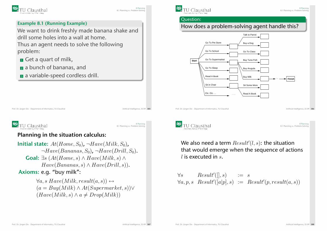
8 Planning8.1 Planning vs. Problem-Solving
Example 8.1 (Running Example)
We want to drink freshly made banana shake anddrill some holes into a wall at home.Thus an agent needs to solve the followingproblem:
1 Get a quart of milk,2 a bunch of bananas, and3 a variable-speed cordless drill.
Prof. Dr. Jürgen Dix · Department of Informatics, TU Clausthal Artificial Intelligence, SS 09 585
8 Planning8.1 Planning vs. Problem-Solving
Question:
How does a problem-solving agent handle this?
. . .
Buy Tuna Fish
Buy Arugula
Buy Milk
Go To Class
Buy a Dog
Talk to Parrot
Sit Some More
Read A Book
...
Go To Supermarket
Go To Sleep
Read A Book
Go To School
Go To Pet Store
Etc. Etc. ...
Sit in Chair
Start
Finish
Prof. Dr. Jürgen Dix · Department of Informatics, TU Clausthal Artificial Intelligence, SS 09 586
8 Planning8.1 Planning vs. Problem-Solving
Planning in the situation calculus:
Initial state: At(Home, S0), ¬Have(Milk, S0),¬Have(Bananas, S0), ¬Have(Drill, S0).
Goal: ∃s (At(Home, s) ∧Have(Milk, s) ∧Have(Bananas, s) ∧Have(Drill, s)).
Axioms: e.g. “buy milk”:
∀a, s Have(Milk, result(a, s))↔(a = Buy(Milk) ∧ At(Supermarket, s))∨(Have(Milk, s) ∧ a 6= Drop(Milk))
Prof. Dr. Jürgen Dix · Department of Informatics, TU Clausthal Artificial Intelligence, SS 09 587
8 Planning8.1 Planning vs. Problem-Solving
We also need a term Result′(l, s): the situationthat would emerge when the sequence of actionsl is executed in s.
∀s Result′([], s) := s∀a, p, s Result′([a|p], s) := Result′(p, result(a, s))
Prof. Dr. Jürgen Dix · Department of Informatics, TU Clausthal Artificial Intelligence, SS 09 588
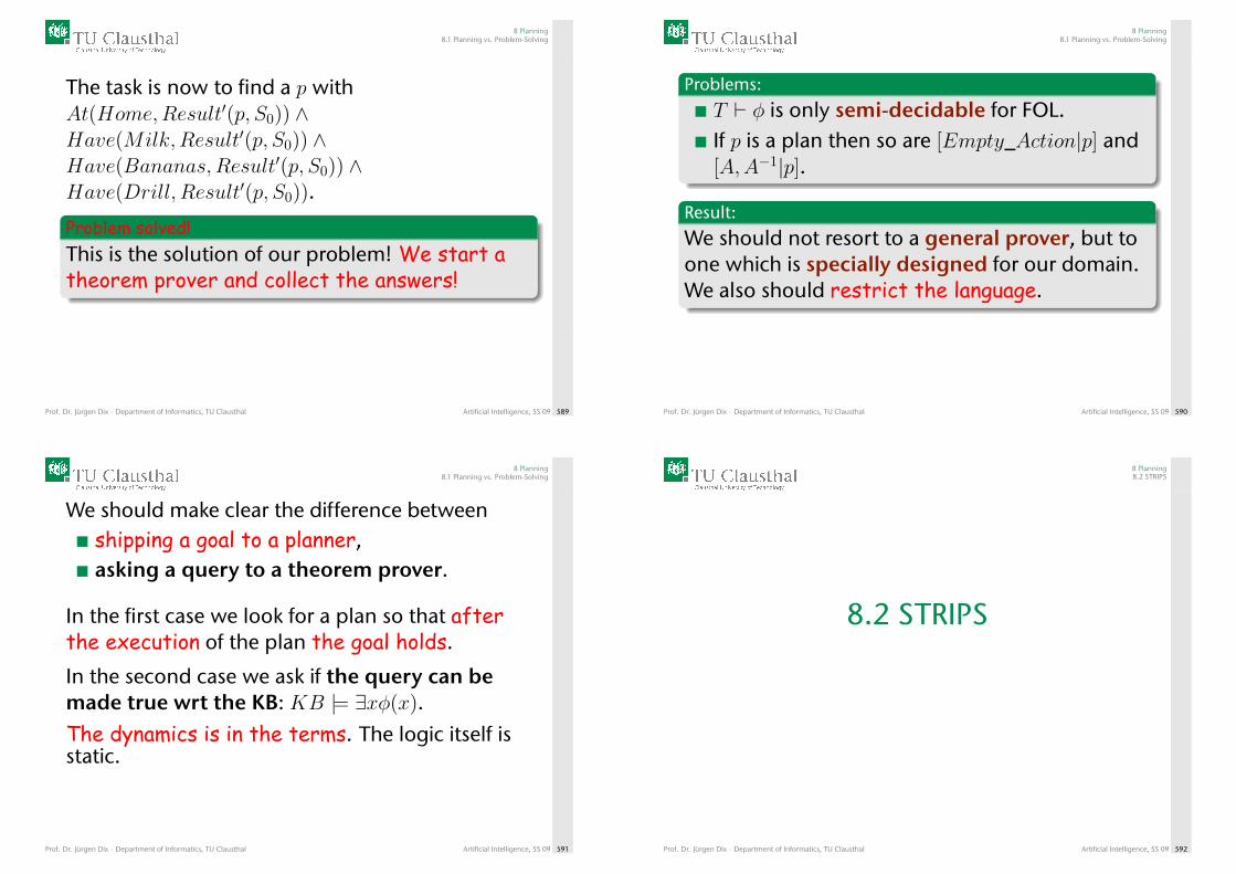
8 Planning8.1 Planning vs. Problem-Solving
The task is now to find a p withAt(Home,Result′(p, S0)) ∧Have(Milk,Result′(p, S0)) ∧Have(Bananas,Result′(p, S0)) ∧Have(Drill, Result′(p, S0)).
Problem solved!This is the solution of our problem! We start atheorem prover and collect the answers!
Prof. Dr. Jürgen Dix · Department of Informatics, TU Clausthal Artificial Intelligence, SS 09 589
8 Planning8.1 Planning vs. Problem-Solving
Problems:
T ` φ is only semi-decidable for FOL.If p is a plan then so are [Empty_Action|p] and[A,A−1|p].
Result:
We should not resort to a general prover, but toone which is specially designed for our domain.We also should restrict the language.
Prof. Dr. Jürgen Dix · Department of Informatics, TU Clausthal Artificial Intelligence, SS 09 590
8 Planning8.1 Planning vs. Problem-Solving
We should make clear the difference betweenshipping a goal to a planner,asking a query to a theorem prover.
In the first case we look for a plan so that afterthe execution of the plan the goal holds.
In the second case we ask if the query can bemade true wrt the KB: KB |= ∃xφ(x).
The dynamics is in the terms. The logic itself isstatic.
Prof. Dr. Jürgen Dix · Department of Informatics, TU Clausthal Artificial Intelligence, SS 09 591
8 Planning8.2 STRIPS
8.2 STRIPS
Prof. Dr. Jürgen Dix · Department of Informatics, TU Clausthal Artificial Intelligence, SS 09 592
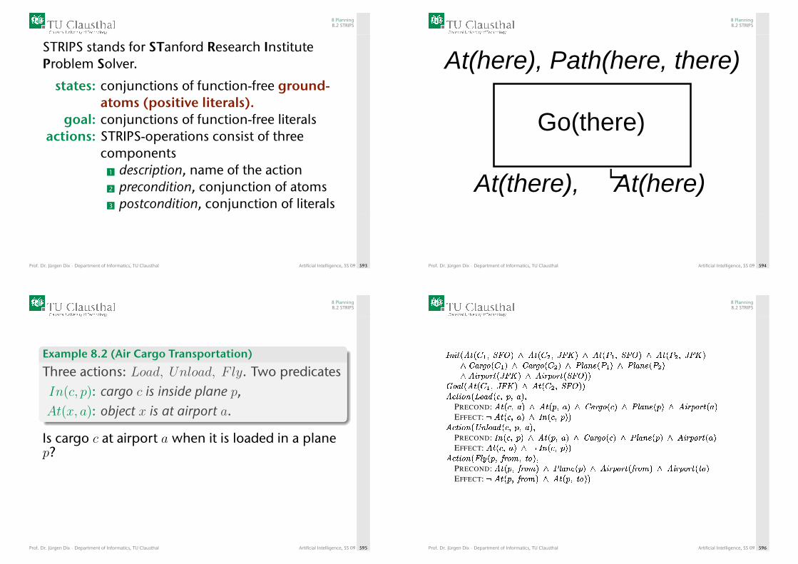
8 Planning8.2 STRIPS
STRIPS stands for STanford Research InstituteProblem Solver.
states: conjunctions of function-free ground-atoms (positive literals).
goal: conjunctions of function-free literalsactions: STRIPS-operations consist of three
components1 description, name of the action2 precondition, conjunction of atoms3 postcondition, conjunction of literals
Prof. Dr. Jürgen Dix · Department of Informatics, TU Clausthal Artificial Intelligence, SS 09 593
8 Planning8.2 STRIPS
At(there), At(here)
Go(there)
L
At(here), Path(here, there)
Prof. Dr. Jürgen Dix · Department of Informatics, TU Clausthal Artificial Intelligence, SS 09 594
8 Planning8.2 STRIPS
Example 8.2 (Air Cargo Transportation)
Three actions: Load, Unload, F ly. Two predicatesIn(c, p): cargo c is inside plane p,At(x, a): object x is at airport a.
Is cargo c at airport a when it is loaded in a planep?
Prof. Dr. Jürgen Dix · Department of Informatics, TU Clausthal Artificial Intelligence, SS 09 595
8 Planning8.2 STRIPS
� � � � � � � � � � � � � � � � � � � � � � � � � � � � � � � � � � � � � � � � � � � �� � � ! # % � � � � � � ! # % � � � � + , � � / � � � � � + , � � / � � � �� � � ! 3 % ! � � � � � � � � � ! 3 % ! � � � � � �
7 % � , � � � � � � � � � � � � � � � � � � � �� ; � � % � � = % � ? � A � C � E � �
PRECOND: � � � A � E � � � � � C � E � � � � ! # % � A � � + , � � / � C � � � � ! 3 % ! � � E �EFFECT: I � � � A � E � � � � � A � C � �
� ; � � % � � J � , % � ? � A � C � E � �PRECOND:
� � � A � C � � � � � C � E � � � � ! # % � A � � + , � � / � C � � � � ! 3 % ! � � E �EFFECT: � � � A � E � � I � � � A � C � �
� ; � � % � � � , M � C � N ! % P � � % � �PRECOND: � � � C � N ! % P � � + , � � / � C � � � � ! 3 % ! � � N ! % P � � � � ! 3 % ! � � � % �EFFECT: I � � � C � N ! % P � � � � � C � � % � �
Prof. Dr. Jürgen Dix · Department of Informatics, TU Clausthal Artificial Intelligence, SS 09 596
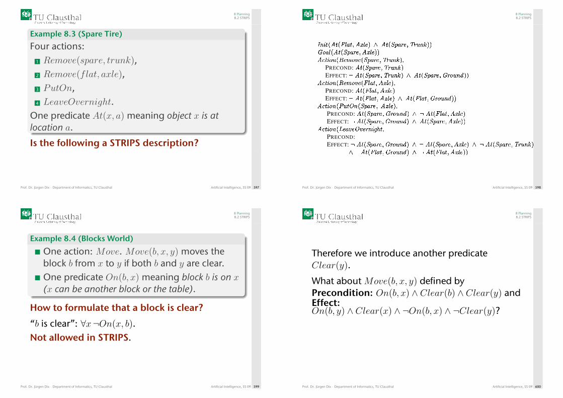
8 Planning8.2 STRIPS
Example 8.3 (Spare Tire)
Four actions:1 Remove(spare, trunk),2 Remove(flat, axle),3 PutOn,4 LeaveOvernight.
One predicate At(x, a) meaning object x is atlocation a.
Is the following a STRIPS description?
Prof. Dr. Jürgen Dix · Department of Informatics, TU Clausthal Artificial Intelligence, SS 09 597
8 Planning8.2 STRIPS
� � � � � � � � � � � � � � � � � � � � � � � � � � � � � ! � �# $ � � � � � � � � � � � � � � � �
� + � � $ � � / � 0 $ 2 � � � � � � � � � � � ! � ,PRECOND: � � � � � � � � � � � � ! �EFFECT: 3 � � � � � � � � � � � � ! � � � � � � � � � � # � $ � � 7 � �
� + � � $ � � / � 0 $ 2 � � � � � � � � � � ,PRECOND: � � � � � � � � � � �EFFECT: 3 � � � � � � � � � � � � � � � � � � # � $ � � 7 � �
� + � � $ � � 8 � � 9 � � � � � � � � � � � � ,PRECOND: � � � � � � � � # � $ � � 7 � � 3 � � � � � � � � � � �EFFECT: 3 � � � � � � � � # � $ � � 7 � � � � � � � � � � � � � � � �
� + � � $ � � < � 2 � 9 2 � � � � = > � ,PRECOND:EFFECT: 3 � � � � � � � � # � $ � � 7 � � 3 � � � � � � � � � � � � � � 3 � � � � � � � � � � � � ! �
� 3 � � � � � � # � $ � � 7 � � 3 � � � � � � � � � � � �
Prof. Dr. Jürgen Dix · Department of Informatics, TU Clausthal Artificial Intelligence, SS 09 598
8 Planning8.2 STRIPS
Example 8.4 (Blocks World)
One action: Move. Move(b, x, y) moves theblock b from x to y if both b and y are clear.One predicate On(b, x) meaning block b is on x(x can be another block or the table).
How to formulate that a block is clear?
“b is clear”: ∀x¬On(x, b).Not allowed in STRIPS.
Prof. Dr. Jürgen Dix · Department of Informatics, TU Clausthal Artificial Intelligence, SS 09 599
8 Planning8.2 STRIPS
Therefore we introduce another predicateClear(y).
What about Move(b, x, y) defined byPrecondition: On(b, x) ∧ Clear(b) ∧ Clear(y) andEffect:On(b, y) ∧ Clear(x) ∧ ¬On(b, x) ∧ ¬Clear(y)?
Prof. Dr. Jürgen Dix · Department of Informatics, TU Clausthal Artificial Intelligence, SS 09 600
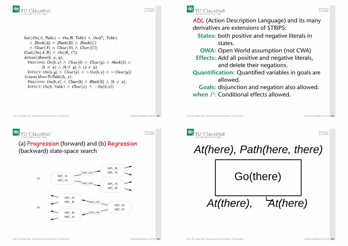
8 Planning8.2 STRIPS
� � � � � � � � � � � � � � � � � � � � � � � � � � � � � � � � � � � � �� " � $ & ' � � � � " � $ & ' � � � � " � $ & ' � � �� * � � � - � � � � * � � � - � � � � * � � � - � � � �
2 $ � � � � � � � � � � � � � � � � �4 & � � $ � � 7 $ 9 � � < = > �
PRECOND: � � � < = � � * � � � - � < � � * � � � - � > � � " � $ & ' � < � �� < @A = � � � < @A > � � � = @A > � ,
EFFECT: � � � < > � � * � � � - � = � � C � � � < = � � C * � � � - � > � �4 & � � $ � � 7 $ 9 � � $ � � � � � � < = �
PRECOND: � � � < = � � * � � � - � < � � " � $ & ' � < � � � < @A = � ,EFFECT: � � � < � � � � � � � * � � � - � = � � C � � � < = � �
Prof. Dr. Jürgen Dix · Department of Informatics, TU Clausthal Artificial Intelligence, SS 09 601
8 Planning8.2 STRIPS
ADL (Action Description Language) and its manyderivatives are extensions of STRIPS:
States: both positive and negative literals instates.
OWA: Open World assumption (not CWA)Effects: Add all positive and negative literals,
and delete their negations.Quantification: Quantified variables in goals are
allowed.Goals: disjunction and negation also allowed.
when P : Conditional effects allowed.
Prof. Dr. Jürgen Dix · Department of Informatics, TU Clausthal Artificial Intelligence, SS 09 602
8 Planning8.2 STRIPS
(a) Progression (forward) and (b) Regression(backward) state-space search
(a)
(b)
2At(P , A)
1At(P , A)
1At(P , A)
2At(P , B)
1At(P , B)
2At(P , A)
1At(P , B)
2At(P , A)
1At(P , A)
2At(P , B)
1At(P , B)
2At(P , B)
1Fly(P ,A,B)
2Fly(P ,A,B)
1Fly(P ,A,B)
2Fly(P ,A,B)
Prof. Dr. Jürgen Dix · Department of Informatics, TU Clausthal Artificial Intelligence, SS 09 603
8 Planning8.2 STRIPS
At(there), At(here)
Go(there)
L
At(here), Path(here, there)
Prof. Dr. Jürgen Dix · Department of Informatics, TU Clausthal Artificial Intelligence, SS 09 604
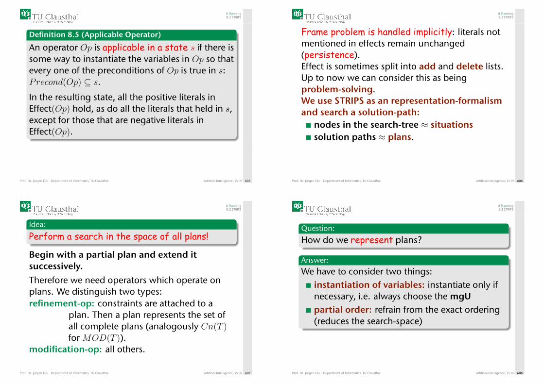
8 Planning8.2 STRIPS
Definition 8.5 (Applicable Operator)
An operator Op is applicable in a state s if there issome way to instantiate the variables in Op so thatevery one of the preconditions of Op is true in s:Precond(Op) ⊆ s.
In the resulting state, all the positive literals inEffect(Op) hold, as do all the literals that held in s,except for those that are negative literals inEffect(Op).
Prof. Dr. Jürgen Dix · Department of Informatics, TU Clausthal Artificial Intelligence, SS 09 605
8 Planning8.2 STRIPS
Frame problem is handled implicitly: literals notmentioned in effects remain unchanged(persistence).Effect is sometimes split into add and delete lists.Up to now we can consider this as beingproblem-solving.We use STRIPS as an representation-formalismand search a solution-path:
nodes in the search-tree ≈ situationssolution paths ≈ plans.
Prof. Dr. Jürgen Dix · Department of Informatics, TU Clausthal Artificial Intelligence, SS 09 606
8 Planning8.2 STRIPS
Idea:
Perform a search in the space of all plans!
Begin with a partial plan and extend itsuccessively.
Therefore we need operators which operate onplans. We distinguish two types:refinement-op: constraints are attached to a
plan. Then a plan represents the set ofall complete plans (analogously Cn(T )for MOD(T )).
modification-op: all others.
Prof. Dr. Jürgen Dix · Department of Informatics, TU Clausthal Artificial Intelligence, SS 09 607
8 Planning8.2 STRIPS
Question:
How do we represent plans?
Answer:
We have to consider two things:instantiation of variables: instantiate only ifnecessary, i.e. always choose the mgUpartial order: refrain from the exact ordering(reduces the search-space)
Prof. Dr. Jürgen Dix · Department of Informatics, TU Clausthal Artificial Intelligence, SS 09 608
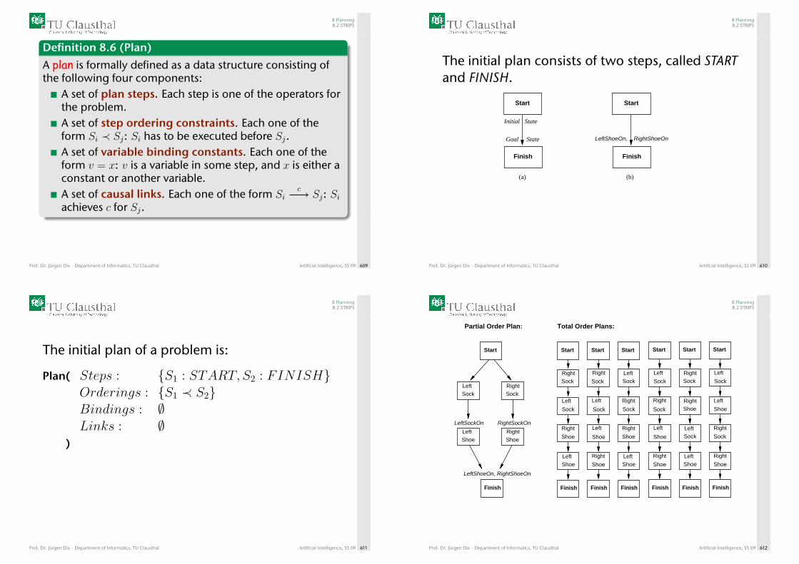
8 Planning8.2 STRIPS
Definition 8.6 (Plan)
A plan is formally defined as a data structure consisting ofthe following four components:
A set of plan steps. Each step is one of the operators forthe problem.A set of step ordering constraints. Each one of theform Si ≺ Sj: Si has to be executed before Sj.A set of variable binding constants. Each one of theform v = x: v is a variable in some step, and x is either aconstant or another variable.A set of causal links. Each one of the form Si
c−→ Sj: Siachieves c for Sj.
Prof. Dr. Jürgen Dix · Department of Informatics, TU Clausthal Artificial Intelligence, SS 09 609
8 Planning8.2 STRIPS
The initial plan consists of two steps, called STARTand FINISH.
Finish
Start
Initial State
Finish
Start
Goal State
(a) (b)
LeftShoeOn, RightShoeOn
Prof. Dr. Jürgen Dix · Department of Informatics, TU Clausthal Artificial Intelligence, SS 09 610
8 Planning8.2 STRIPS
The initial plan of a problem is:
Plan( Steps : {S1 : START, S2 : FINISH}Orderings : {S1 ≺ S2}Bindings : ∅Links : ∅
)
Prof. Dr. Jürgen Dix · Department of Informatics, TU Clausthal Artificial Intelligence, SS 09 611
8 Planning8.2 STRIPS
StartStartStart
Total Order Plans: Partial Order Plan:
Start
Left
Sock
Left
Shoe
Sock
Right
Shoe
Right
Finish
Start
Finish
SockRight
ShoeRight
SockLeft
ShoeLeft
Start
Left
Sock
Shoe
Right
Finish
Right
Sock
Left
Shoe
Finish
SockLeft
Right
Sock
ShoeLeft
Right
Shoe
Shoe
Right
Finish
Sock
Right
Left
Sock
Left
Shoe
Finish
SockRight
ShoeLeft
Left
Sock
Right
Shoe
LeftSockOn RightSockOn
LeftShoeOn, RightShoeOn
Start
SockRight
ShoeRight
SockLeft
ShoeLeft
Finish
Prof. Dr. Jürgen Dix · Department of Informatics, TU Clausthal Artificial Intelligence, SS 09 612
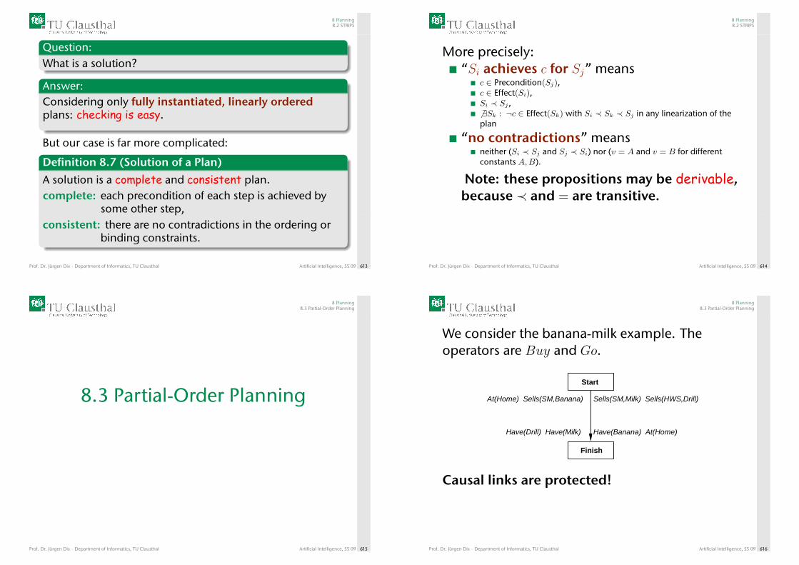
8 Planning8.2 STRIPS
Question:What is a solution?
Answer:Considering only fully instantiated, linearly orderedplans: checking is easy.
But our case is far more complicated:
Definition 8.7 (Solution of a Plan)
A solution is a complete and consistent plan.complete: each precondition of each step is achieved by
some other step,consistent: there are no contradictions in the ordering or
binding constraints.
Prof. Dr. Jürgen Dix · Department of Informatics, TU Clausthal Artificial Intelligence, SS 09 613
8 Planning8.2 STRIPS
More precisely:“Si achieves c for Sj” means
c ∈ Precondition(Sj),c ∈ Effect(Si),Si ≺ Sj ,6 ∃Sk : ¬c ∈ Effect(Sk) with Si ≺ Sk ≺ Sj in any linearization of theplan
“no contradictions” meansneither (Si ≺ Sj and Sj ≺ Si) nor (v = A and v = B for differentconstants A,B).
Note: these propositions may be derivable,because ≺ and = are transitive.
Prof. Dr. Jürgen Dix · Department of Informatics, TU Clausthal Artificial Intelligence, SS 09 614
8 Planning8.3 Partial-Order Planning
8.3 Partial-Order Planning
Prof. Dr. Jürgen Dix · Department of Informatics, TU Clausthal Artificial Intelligence, SS 09 615
8 Planning8.3 Partial-Order Planning
We consider the banana-milk example. Theoperators are Buy and Go.
Finish
Start
Have(Drill) Have(Milk) Have(Banana) At(Home)
At(Home) Sells(SM,Banana) Sells(SM,Milk) Sells(HWS,Drill)
Causal links are protected!
Prof. Dr. Jürgen Dix · Department of Informatics, TU Clausthal Artificial Intelligence, SS 09 616
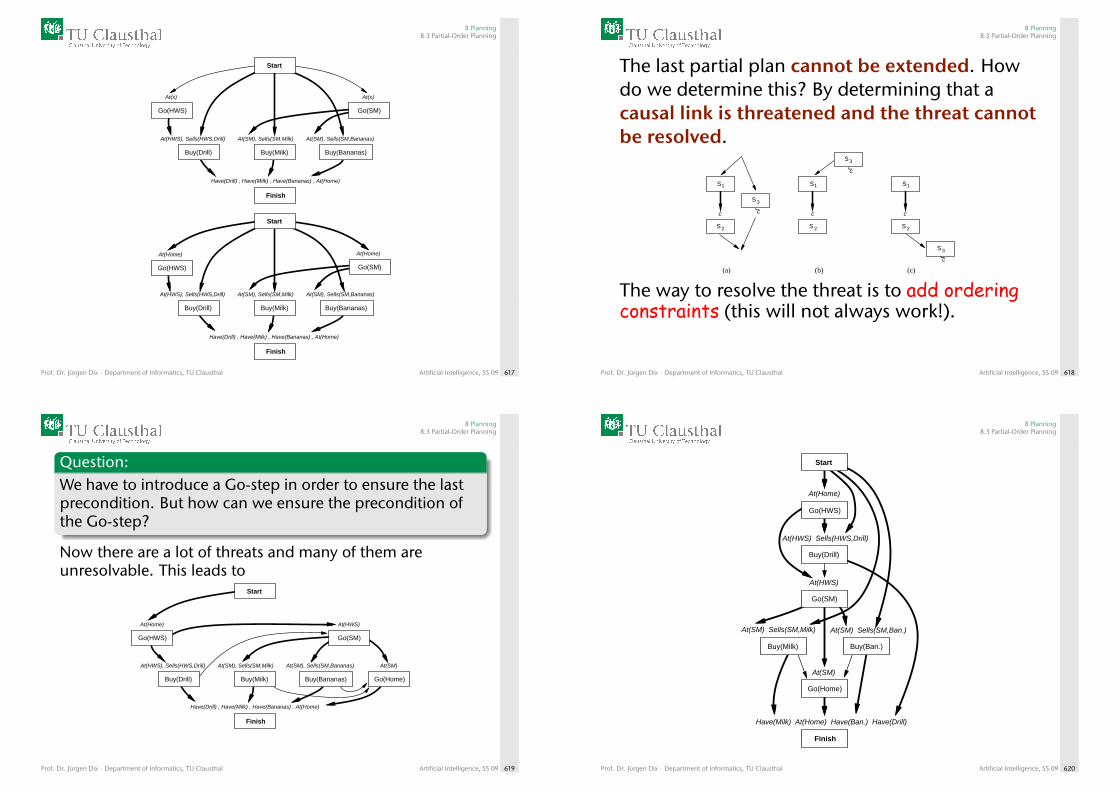
8 Planning8.3 Partial-Order Planning
At(SM), Sells(SM,Bananas)At(SM), Sells(SM,Milk)
At(x)At(x)
At(HWS), Sells(HWS,Drill)
Have(Drill) , Have(Milk) , Have(Bananas) , At(Home)
Finish
Go(HWS)
Buy(Drill) Buy(Milk) Buy(Bananas)
Go(SM)
Start
At(SM), Sells(SM,Bananas)At(SM), Sells(SM,Milk)At(HWS), Sells(HWS,Drill)
Have(Drill) , Have(Milk) , Have(Bananas) , At(Home)
Finish
Go(HWS)
Buy(Drill) Buy(Milk) Buy(Bananas)
Go(SM)
Start
At(Home) At(Home)
Prof. Dr. Jürgen Dix · Department of Informatics, TU Clausthal Artificial Intelligence, SS 09 617
8 Planning8.3 Partial-Order Planning
The last partial plan cannot be extended. Howdo we determine this? By determining that acausal link is threatened and the threat cannotbe resolved.
cL
cL
cLc cc
(a) (b) (c)
S 2
S 3
S 2
S 3
S 2
S 3
S1S11S
The way to resolve the threat is to add orderingconstraints (this will not always work!).
Prof. Dr. Jürgen Dix · Department of Informatics, TU Clausthal Artificial Intelligence, SS 09 618
8 Planning8.3 Partial-Order Planning
Question:We have to introduce a Go-step in order to ensure the lastprecondition. But how can we ensure the precondition ofthe Go-step?
Now there are a lot of threats and many of them areunresolvable. This leads to
At(SM), Sells(SM,Bananas)At(SM), Sells(SM,Milk)At(HWS), Sells(HWS,Drill)
Have(Drill) , Have(Milk) , Have(Bananas) , At(Home)
At(Home) At(HWS)
At(SM)
Finish
Go(HWS)
Buy(Drill) Buy(Milk) Buy(Bananas)
Go(SM)
Start
Go(Home)
Prof. Dr. Jürgen Dix · Department of Informatics, TU Clausthal Artificial Intelligence, SS 09 619
8 Planning8.3 Partial-Order Planning
At(SM)
At(Home)
At(HWS)
Have(Milk) At(Home) Have(Ban.) Have(Drill)
Buy(Drill)
Buy(Milk) Buy(Ban.)
Go(Home)
Go(HWS)
Go(SM)
Finish
Start
At(HWS) Sells(HWS,Drill)
At(SM) Sells(SM,Milk) At(SM) Sells(SM,Ban.)
Prof. Dr. Jürgen Dix · Department of Informatics, TU Clausthal Artificial Intelligence, SS 09 620
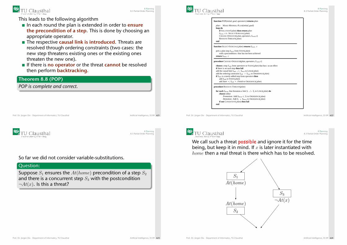
8 Planning8.3 Partial-Order Planning
This leads to the following algorithmIn each round the plan is extended in order to ensurethe precondition of a step. This is done by choosing anappropriate operator.The respective causal link is introduced. Threats areresolved through ordering constraints (two cases: thenew step threatens existing ones or the existing onesthreaten the new one).If there is no operator or the threat cannot be resolvedthen perform backtracking.
Theorem 8.8 (POP)POP is complete and correct.
Prof. Dr. Jürgen Dix · Department of Informatics, TU Clausthal Artificial Intelligence, SS 09 621
8 Planning8.3 Partial-Order Planning
function POP(initial, goal, operators) returns plan
plan�MAKE-MINIMAL-PLAN(initial, goal)loop do
if SOLUTION?( plan) then return planSneed, c� SELECT-SUBGOAL( plan)CHOOSE-OPERATOR( plan, operators, Sneed, c)RESOLVE-THREATS( plan)
end
function SELECT-SUBGOAL( plan) returns Sneed, c
pick a plan step Sneed from STEPS( plan)with a precondition c that has not been achieved
return Sneed, c
procedure CHOOSE-OPERATOR(plan, operators, S need, c)
choose a step Sadd from operators or STEPS( plan) that has c as an effectif there is no such step then failadd the causal link Sadd
c�� Sneed to LINKS( plan)
add the ordering constraint Sadd � Sneed to ORDERINGS( plan)if Sadd is a newly added step from operators then
add Sadd to STEPS( plan)add Start � Sadd � Finish to ORDERINGS( plan)
procedure RESOLVE-THREATS(plan)
for each Sthreat that threatens a link Sic�� Sj in LINKS( plan) do
choose eitherPromotion: Add Sthreat� Si to ORDERINGS( plan)Demotion: Add Sj � Sthreat to ORDERINGS( plan)
if not CONSISTENT( plan) then failend
Prof. Dr. Jürgen Dix · Department of Informatics, TU Clausthal Artificial Intelligence, SS 09 622
8 Planning8.3 Partial-Order Planning
So far we did not consider variable-substitutions.
Question:Suppose S1 ensures the At(home) precondition of a step S2
and there is a concurrent step S3 with the postcondition¬At(x). Is this a threat?
Prof. Dr. Jürgen Dix · Department of Informatics, TU Clausthal Artificial Intelligence, SS 09 623
8 Planning8.3 Partial-Order Planning
We call such a threat possible and ignore it for the timebeing, but keep it in mind. If x is later instantiated withhome then a real threat is there which has to be resolved.
S1
At(home)
S2
At(home)
S3
¬At(x )
Prof. Dr. Jürgen Dix · Department of Informatics, TU Clausthal Artificial Intelligence, SS 09 624
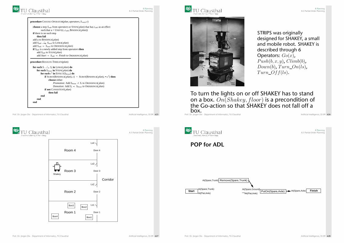
8 Planning8.3 Partial-Order Planning
procedure CHOOSE-OPERATOR(plan, operators, S need, c)
choose a step Sadd from operators or STEPS( plan) that has cadd as an effectsuch that u = UNIFY(c, cadd, BINDINGS( plan))
if there is no such stepthen fail
add u to BINDINGS( plan)add Sadd
c�� Sneed to LINKS( plan)
add Sadd � Sneed to ORDERINGS( plan)if Sadd is a newly added step from operators then
add Sadd to STEPS( plan)add Start � Sadd � Finish to ORDERINGS( plan)
procedure RESOLVE-THREATS(plan)
for each Sic�� Sj in LINKS( plan) do
for each Sthreat in STEPS( plan) dofor each c� in EFFECT(Sthreat) do
if SUBST(BINDINGS( plan), c) = SUBST(BINDINGS( plan),� c�) thenchoose either
Promotion: Add Sthreat � Si to ORDERINGS( plan)Demotion: Add Sj � Sthreat to ORDERINGS( plan)
if not CONSISTENT( plan)then fail
endend
end
Prof. Dr. Jürgen Dix · Department of Informatics, TU Clausthal Artificial Intelligence, SS 09 625
8 Planning8.3 Partial-Order Planning
STRIPS was originallydesigned for SHAKEY, a smalland mobile robot. SHAKEY isdescribed through 6Operators: Go(x),Push(b, x, y), Climb(b),Down(b), Turn_On(ls),Turn_Off(ls).
To turn the lights on or off SHAKEY has to standon a box. On(Shakey, floor) is a precondition ofthe Go-action so that SHAKEY does not fall off abox.
Prof. Dr. Jürgen Dix · Department of Informatics, TU Clausthal Artificial Intelligence, SS 09 626
8 Planning8.3 Partial-Order Planning
Room 4
Room 3
Room 2
Room 1 Door 1
Door 2
Door 3
Door 4
Box1
Box2Box3
Shakey
Ls1
Ls2
Ls3
Ls4
Box4
Corridor
Prof. Dr. Jürgen Dix · Department of Informatics, TU Clausthal Artificial Intelligence, SS 09 627
8 Planning8.3 Partial-Order Planning
POP for ADL
Remove(Spare,Trunk)At(Spare,Trunk)
PutOn(Spare,Axle)At(Spare,Ground)
At(Flat,Axle)FinishAt(Spare,Axle)Start
At(Flat,Axle)
At(Spare,Trunk)
Prof. Dr. Jürgen Dix · Department of Informatics, TU Clausthal Artificial Intelligence, SS 09 628
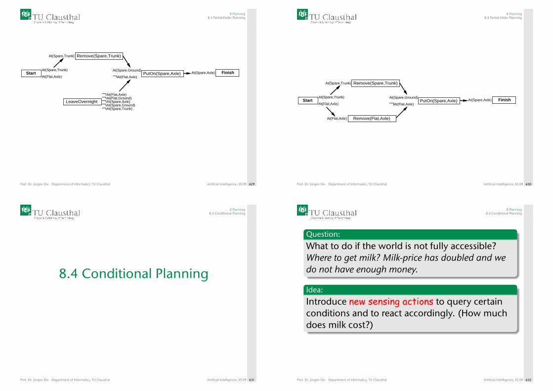
8 Planning8.3 Partial-Order Planning
Remove(Spare,Trunk)At(Spare,Trunk)
PutOn(Spare,Axle)At(Spare,Ground)
At(Flat,Axle)FinishAt(Spare,Axle)
LeaveOvernight
At(Flat,Axle)At(Flat,Ground)At(Spare,Axle)At(Spare,Ground)At(Spare,Trunk)
StartAt(Flat,Axle)
At(Spare,Trunk)
Prof. Dr. Jürgen Dix · Department of Informatics, TU Clausthal Artificial Intelligence, SS 09 629
8 Planning8.3 Partial-Order Planning
Start
Remove(Spare,Trunk)At(Spare,Trunk)
Remove(Flat,Axle)At(Flat,Axle)
PutOn(Spare,Axle)At(Spare,Ground)
At(Flat,Axle)FinishAt(Spare,Axle)
At(Flat,Axle)
At(Spare,Trunk)
Prof. Dr. Jürgen Dix · Department of Informatics, TU Clausthal Artificial Intelligence, SS 09 630
8 Planning8.4 Conditional Planning
8.4 Conditional Planning
Prof. Dr. Jürgen Dix · Department of Informatics, TU Clausthal Artificial Intelligence, SS 09 631
8 Planning8.4 Conditional Planning
Question:
What to do if the world is not fully accessible?Where to get milk? Milk-price has doubled and wedo not have enough money.
Idea:
Introduce new sensing actions to query certainconditions and to react accordingly. (How muchdoes milk cost?)
Prof. Dr. Jürgen Dix · Department of Informatics, TU Clausthal Artificial Intelligence, SS 09 632
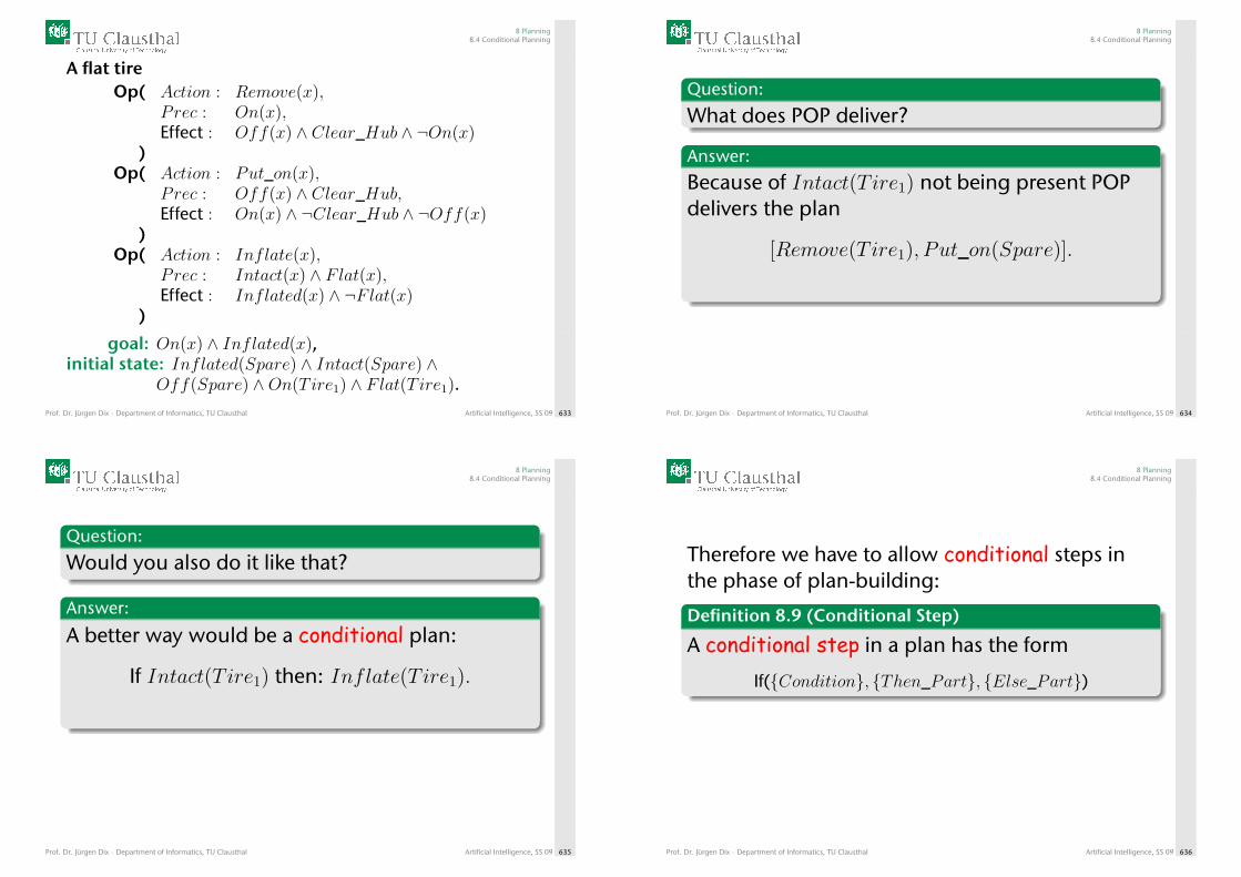
8 Planning8.4 Conditional Planning
A flat tireOp( Action : Remove(x),
P rec : On(x),Effect : Off(x) ∧ Clear_Hub ∧ ¬On(x)
)Op( Action : Put_on(x),
P rec : Off(x) ∧ Clear_Hub,Effect : On(x) ∧ ¬Clear_Hub ∧ ¬Off(x)
)Op( Action : Inflate(x),
P rec : Intact(x) ∧ Flat(x),Effect : Inflated(x) ∧ ¬Flat(x)
)
goal: On(x) ∧ Inflated(x),initial state: Inflated(Spare) ∧ Intact(Spare) ∧
Off(Spare) ∧On(Tire1) ∧ Flat(Tire1).Prof. Dr. Jürgen Dix · Department of Informatics, TU Clausthal Artificial Intelligence, SS 09 633
8 Planning8.4 Conditional Planning
Question:
What does POP deliver?
Answer:
Because of Intact(Tire1) not being present POPdelivers the plan
[Remove(Tire1), Put_on(Spare)].
Prof. Dr. Jürgen Dix · Department of Informatics, TU Clausthal Artificial Intelligence, SS 09 634
8 Planning8.4 Conditional Planning
Question:
Would you also do it like that?
Answer:
A better way would be a conditional plan:
If Intact(Tire1) then: Inflate(Tire1).
Prof. Dr. Jürgen Dix · Department of Informatics, TU Clausthal Artificial Intelligence, SS 09 635
8 Planning8.4 Conditional Planning
Therefore we have to allow conditional steps inthe phase of plan-building:
Definition 8.9 (Conditional Step)
A conditional step in a plan has the form
If({Condition}, {Then_Part}, {Else_Part})
Prof. Dr. Jürgen Dix · Department of Informatics, TU Clausthal Artificial Intelligence, SS 09 636
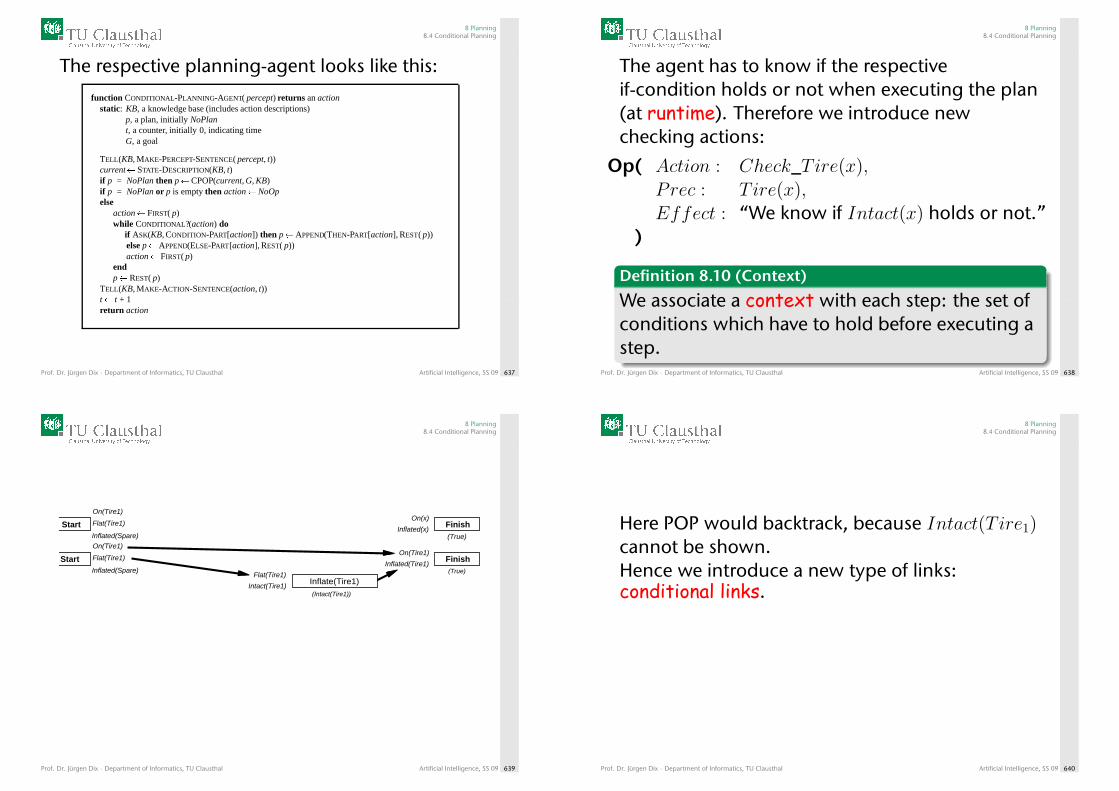
8 Planning8.4 Conditional Planning
The respective planning-agent looks like this:
function CONDITIONAL-PLANNING-AGENT( percept) returns an actionstatic: KB, a knowledge base (includes action descriptions)
p, a plan, initially NoPlant, a counter, initially 0, indicating timeG, a goal
TELL(KB, MAKE-PERCEPT-SENTENCE( percept, t))current� STATE-DESCRIPTION(KB, t)if p = NoPlan then p�CPOP(current, G, KB)if p = NoPlan or p is empty then action�NoOpelse
action� FIRST( p)while CONDITIONAL?(action) do
if ASK(KB, CONDITION-PART[action]) then p�APPEND(THEN-PART[action], REST( p))else p�APPEND(ELSE-PART[action], REST( p))action� FIRST( p)
endp�REST( p)
TELL(KB, MAKE-ACTION-SENTENCE(action, t))t� t + 1return action
Prof. Dr. Jürgen Dix · Department of Informatics, TU Clausthal Artificial Intelligence, SS 09 637
8 Planning8.4 Conditional Planning
The agent has to know if the respectiveif-condition holds or not when executing the plan(at runtime). Therefore we introduce newchecking actions:
Op( Action : Check_Tire(x),P rec : Tire(x),Effect : “We know if Intact(x) holds or not.”
)
Definition 8.10 (Context)
We associate a context with each step: the set ofconditions which have to hold before executing astep.
Prof. Dr. Jürgen Dix · Department of Informatics, TU Clausthal Artificial Intelligence, SS 09 638
8 Planning8.4 Conditional Planning
Inflated(Spare)
On(Tire1)
Flat(Tire1)Start Finish(True)
Inflated(x)
On(x)
(Intact(Tire1))
Inflated(Spare)
On(Tire1)
Flat(Tire1)On(Tire1)
Inflated(Tire1)
Flat(Tire1)
Intact(Tire1)
Start Finish
Inflate(Tire1)(True)
Prof. Dr. Jürgen Dix · Department of Informatics, TU Clausthal Artificial Intelligence, SS 09 639
8 Planning8.4 Conditional Planning
Here POP would backtrack, because Intact(Tire1)cannot be shown.Hence we introduce a new type of links:conditional links.
Prof. Dr. Jürgen Dix · Department of Informatics, TU Clausthal Artificial Intelligence, SS 09 640
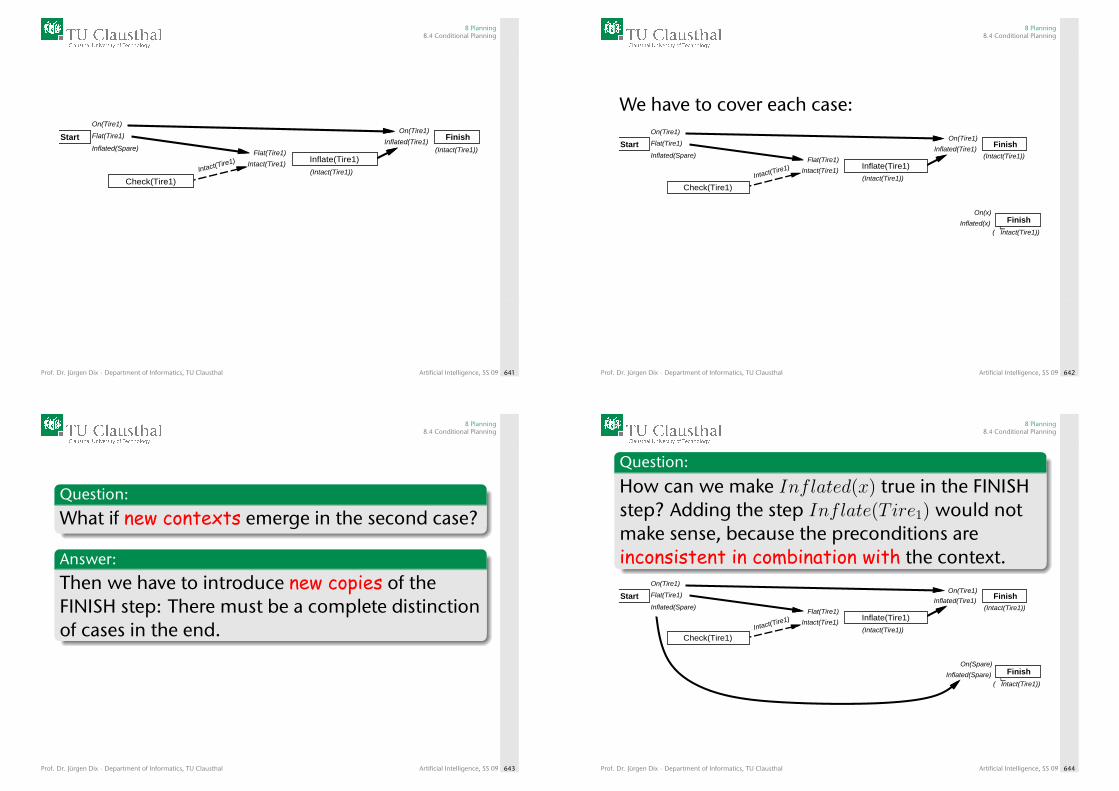
8 Planning8.4 Conditional Planning
(Intact(Tire1))
Inflated(Spare)
On(Tire1)
Flat(Tire1)
Intact(Tire1)
On(Tire1)
Inflated(Tire1)(Intact(Tire1))Flat(Tire1)
Intact(Tire1)
Start Finish
Check(Tire1)
Inflate(Tire1)
Prof. Dr. Jürgen Dix · Department of Informatics, TU Clausthal Artificial Intelligence, SS 09 641
8 Planning8.4 Conditional Planning
We have to cover each case:
( Intact(Tire1))L
(Intact(Tire1))
Inflated(Spare)
On(Tire1)
Flat(Tire1)
Intact(Tire1)
On(Tire1)
Inflated(Tire1)(Intact(Tire1))Flat(Tire1)
Intact(Tire1)
Start Finish
Finish
Check(Tire1)
Inflate(Tire1)
On(x)
Inflated(x)
Prof. Dr. Jürgen Dix · Department of Informatics, TU Clausthal Artificial Intelligence, SS 09 642
8 Planning8.4 Conditional Planning
Question:
What if new contexts emerge in the second case?
Answer:
Then we have to introduce new copies of theFINISH step: There must be a complete distinctionof cases in the end.
Prof. Dr. Jürgen Dix · Department of Informatics, TU Clausthal Artificial Intelligence, SS 09 643
8 Planning8.4 Conditional Planning
Question:
How can we make Inflated(x) true in the FINISHstep? Adding the step Inflate(Tire1) would notmake sense, because the preconditions areinconsistent in combination with the context.
( Intact(Tire1))L
On(Spare)
Inflated(Spare)
(Intact(Tire1))
Inflated(Spare)
On(Tire1)
Flat(Tire1)
Intact(Tire1)
On(Tire1)
Inflated(Tire1)(Intact(Tire1))Flat(Tire1)
Intact(Tire1)
Start Finish
Finish
Check(Tire1)
Inflate(Tire1)
Prof. Dr. Jürgen Dix · Department of Informatics, TU Clausthal Artificial Intelligence, SS 09 644
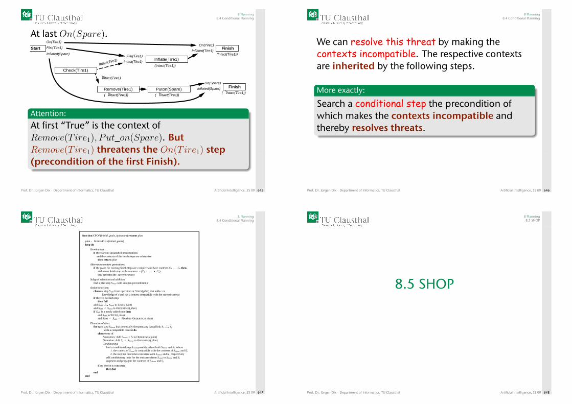
8 Planning8.4 Conditional Planning
At last On(Spare).
( Intact(Tire1))L
On(Spare)
Inflated(Spare)
(Intact(Tire1))
On(Tire1)
Inflated(Tire1)(Intact(Tire1))
( Intact(Tire1))L
( Intact(Tire1))L
Inflated(Spare)
On(Tire1)
Flat(Tire1)
Intact(Tire1)Flat(Tire1)
Intact(Tire1)
Start Finish
FinishPuton(Spare)
Check(Tire1)
Remove(Tire1)
Inflate(Tire1)
Intact(Tire1)L
Attention:
At first “True” is the context ofRemove(Tire1), Put_on(Spare). ButRemove(Tire1) threatens the On(Tire1) step(precondition of the first Finish).
Prof. Dr. Jürgen Dix · Department of Informatics, TU Clausthal Artificial Intelligence, SS 09 645
8 Planning8.4 Conditional Planning
We can resolve this threat by making thecontexts incompatible. The respective contextsare inherited by the following steps.
More exactly:
Search a conditional step the precondition ofwhich makes the contexts incompatible andthereby resolves threats.
Prof. Dr. Jürgen Dix · Department of Informatics, TU Clausthal Artificial Intelligence, SS 09 646
8 Planning8.4 Conditional Planning
function CPOP(initial, goals, operators) returns plan
plan�MAKE-PLAN(initial, goals)loop do
Termination:if there are no unsatisfied preconditions
and the contexts of the finish steps are exhaustivethen return plan
Alternative context generation:if the plans for existing finish steps are complete and have contexts C 1 . . . Cn then
add a new finish step with a context � (C1 � . . . � Cn)this becomes the current context
Subgoal selection and addition:find a plan step Sneed with an open precondition c
Action selection:choose a step Sadd from operators or STEPS( plan) that adds c or
knowledge of c and has a context compatible with the current contextif there is no such step
then failadd Sadd
c�� Sneed to LINKS( plan)
add Sadd < Sneed to ORDERINGS( plan)if Sadd is a newly added step then
add Sadd to STEPS( plan)add Start < Sadd < Finish to ORDERINGS( plan)
Threat resolution:for each step Sthreat that potentially threatens any causal link Si
c�� Sj
with a compatible context dochoose one of
Promotion: Add Sthreat < Si to ORDERINGS( plan)Demotion: Add Sj < Sthreat to ORDERINGS( plan)Conditioning:
find a conditional step Scond possibly before both Sthreat and Sj, where1. the context of Scond is compatible with the contexts of Sthreat and Sj;2. the step has outcomes consistent with Sthreat and Sj, respectively
add conditioning links for the outcomes from Scond to Sthreat and Sj
augment and propagate the contexts of S threat and Sj
if no choice is consistentthen fail
endend
Prof. Dr. Jürgen Dix · Department of Informatics, TU Clausthal Artificial Intelligence, SS 09 647
8 Planning8.5 SHOP
8.5 SHOP
Prof. Dr. Jürgen Dix · Department of Informatics, TU Clausthal Artificial Intelligence, SS 09 648
8 Planning8.5 SHOP
Up to now: Action-based planning (POP,CPOP)
Each state of the world is represented by a setof atoms, and each action corresponds to adeterministic state transition.Search space is still huge.HTN planning has been proved to be moreexpressive than action-based planning.Moreover, HTN planning algorithms havebeen experimentally proved to be moreefficient than their action-based counterparts.
Prof. Dr. Jürgen Dix · Department of Informatics, TU Clausthal Artificial Intelligence, SS 09 649
8 Planning8.5 SHOP
HTN-Planning
Each state of the world is represented by a setof atoms, and each action corresponds to adeterministic state transition.Hierarchical Task Networks: HTN plannersdiffer from classical planners in what they planfor, and how they plan for it.
Prof. Dr. Jürgen Dix · Department of Informatics, TU Clausthal Artificial Intelligence, SS 09 650
8 Planning8.5 SHOP
HTN-Planning (2)
Classical HTN planning (dating back to mid-70ies)focused on particular application domains:production-line scheduling, crisis management andlogistics, planning and scheduling for spacecraft,equipment configuration, manufacturability analysis,evacuation planning, and the game of bridge.There are also domain-independent HTN planners:Nonlin, Sipe-2 , O-Plan, UMCP , SHOP , ASHOP , andSHOP2 .We focus on SHOP .
Prof. Dr. Jürgen Dix · Department of Informatics, TU Clausthal Artificial Intelligence, SS 09 651
8 Planning8.5 SHOP
Features of HTN planning
Why is HTN planning superior to classicalaction-based planning?The domain knowledge and the notion ofdecomposing a task network while satisfyingthe given constraints enable the planner tofocus on a much smaller portion of thesearch space.
Prof. Dr. Jürgen Dix · Department of Informatics, TU Clausthal Artificial Intelligence, SS 09 652
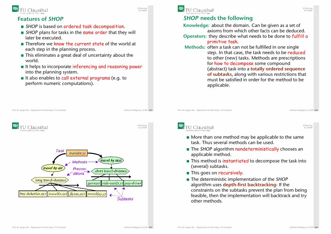
8 Planning8.5 SHOP
Features of SHOPSHOP is based on ordered task decomposition.SHOP plans for tasks in the same order that they willlater be executed.Therefore we know the current state of the world ateach step in the planning process.This eliminates a great deal of uncertainty about theworld.It helps to incorporate inferencing and reasoning powerinto the planning system.It also enables to call external programs (e.g. toperform numeric computations).
Prof. Dr. Jürgen Dix · Department of Informatics, TU Clausthal Artificial Intelligence, SS 09 653
8 Planning8.5 SHOP
SHOP needs the followingKnowledge: about the domain. Can be given as a set of
axioms from which other facts can be deduced.Operators: they describe what needs to be done to fulfill a
primitive task.Methods: often a task can not be fulfilled in one single
step. In that case, the task needs to be reducedto other (new) tasks. Methods are prescriptionsfor how to decompose some compound(abstract) task into a totally ordered sequenceof subtasks, along with various restrictions thatmust be satisfied in order for the method to beapplicable.
Prof. Dr. Jürgen Dix · Department of Informatics, TU Clausthal Artificial Intelligence, SS 09 654
8 Planning8.5 SHOP
Prof. Dr. Jürgen Dix · Department of Informatics, TU Clausthal Artificial Intelligence, SS 09 655
8 Planning8.5 SHOP
More than one method may be applicable to the sametask. Thus several methods can be used.The SHOP algorithm nondeterministically chooses anapplicable method.This method is instantiated to decompose the task into(several) subtasks.This goes on recursively.The deterministic implementation of the SHOPalgorithm uses depth-first backtracking: If theconstraints on the subtasks prevent the plan from beingfeasible, then the implementation will backtrack and tryother methods.
Prof. Dr. Jürgen Dix · Department of Informatics, TU Clausthal Artificial Intelligence, SS 09 656
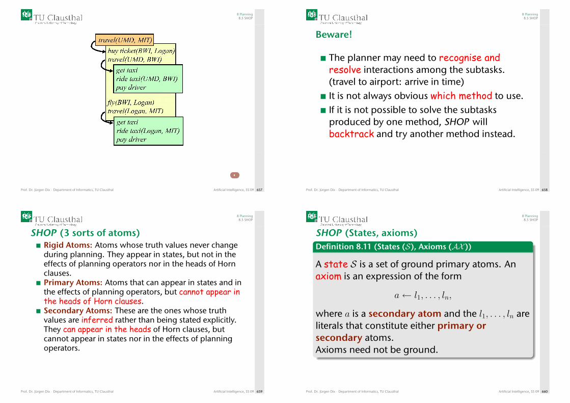
8 Planning8.5 SHOP
Prof. Dr. Jürgen Dix · Department of Informatics, TU Clausthal Artificial Intelligence, SS 09 657
8 Planning8.5 SHOP
Beware!
The planner may need to recognise andresolve interactions among the subtasks.(travel to airport: arrive in time)It is not always obvious which method to use.If it is not possible to solve the subtasksproduced by one method, SHOP willbacktrack and try another method instead.
Prof. Dr. Jürgen Dix · Department of Informatics, TU Clausthal Artificial Intelligence, SS 09 658
8 Planning8.5 SHOP
SHOP (3 sorts of atoms)Rigid Atoms: Atoms whose truth values never changeduring planning. They appear in states, but not in theeffects of planning operators nor in the heads of Hornclauses.Primary Atoms: Atoms that can appear in states and inthe effects of planning operators, but cannot appear inthe heads of Horn clauses.Secondary Atoms: These are the ones whose truthvalues are inferred rather than being stated explicitly.They can appear in the heads of Horn clauses, butcannot appear in states nor in the effects of planningoperators.
Prof. Dr. Jürgen Dix · Department of Informatics, TU Clausthal Artificial Intelligence, SS 09 659
8 Planning8.5 SHOP
SHOP (States, axioms)Definition 8.11 (States (S), Axioms (AX ))
A state S is a set of ground primary atoms. Anaxiom is an expression of the form
a← l1, . . . , ln,
where a is a secondary atom and the l1, . . . , ln areliterals that constitute either primary orsecondary atoms.Axioms need not be ground.
Prof. Dr. Jürgen Dix · Department of Informatics, TU Clausthal Artificial Intelligence, SS 09 660
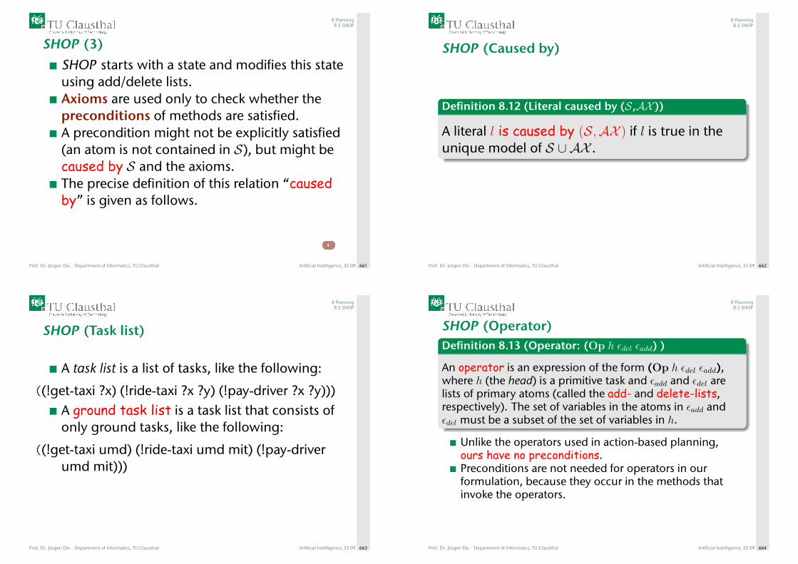
8 Planning8.5 SHOP
SHOP (3)
SHOP starts with a state and modifies this stateusing add/delete lists.Axioms are used only to check whether thepreconditions of methods are satisfied.A precondition might not be explicitly satisfied(an atom is not contained in S), but might becaused by S and the axioms.The precise definition of this relation “causedby” is given as follows.
Prof. Dr. Jürgen Dix · Department of Informatics, TU Clausthal Artificial Intelligence, SS 09 661
8 Planning8.5 SHOP
SHOP (Caused by)
Definition 8.12 (Literal caused by (S,AX ))
A literal l is caused by (S,AX ) if l is true in theunique model of S ∪ AX .
Prof. Dr. Jürgen Dix · Department of Informatics, TU Clausthal Artificial Intelligence, SS 09 662
8 Planning8.5 SHOP
SHOP (Task list)
A task list is a list of tasks, like the following:
((!get-taxi ?x) (!ride-taxi ?x ?y) (!pay-driver ?x ?y)))A ground task list is a task list that consists ofonly ground tasks, like the following:
((!get-taxi umd) (!ride-taxi umd mit) (!pay-driverumd mit)))
Prof. Dr. Jürgen Dix · Department of Informatics, TU Clausthal Artificial Intelligence, SS 09 663
8 Planning8.5 SHOP
SHOP (Operator)Definition 8.13 (Operator: (Op h εdel εadd) )
An operator is an expression of the form (Op h εdel εadd),where h (the head) is a primitive task and εadd and εdel arelists of primary atoms (called the add- and delete-lists,respectively). The set of variables in the atoms in εadd andεdel must be a subset of the set of variables in h.
Unlike the operators used in action-based planning,ours have no preconditions.Preconditions are not needed for operators in ourformulation, because they occur in the methods thatinvoke the operators.
Prof. Dr. Jürgen Dix · Department of Informatics, TU Clausthal Artificial Intelligence, SS 09 664
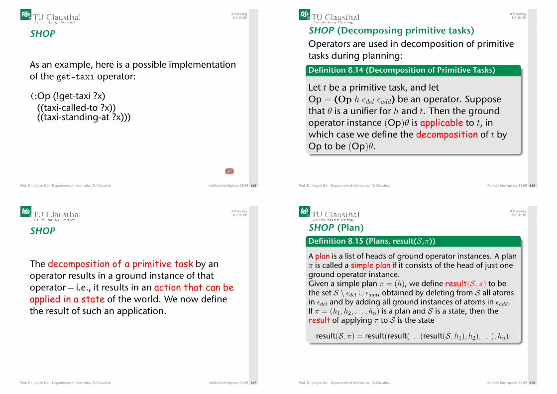
8 Planning8.5 SHOP
SHOP
As an example, here is a possible implementationof the get-taxi operator:
(:Op (!get-taxi ?x)((taxi-called-to ?x))((taxi-standing-at ?x)))
Prof. Dr. Jürgen Dix · Department of Informatics, TU Clausthal Artificial Intelligence, SS 09 665
8 Planning8.5 SHOP
SHOP (Decomposing primitive tasks)Operators are used in decomposition of primitivetasks during planning:Definition 8.14 (Decomposition of Primitive Tasks)
Let t be a primitive task, and letOp = (Op h εdel εadd) be an operator. Supposethat θ is a unifier for h and t. Then the groundoperator instance (Op)θ is applicable to t, inwhich case we define the decomposition of t byOp to be (Op)θ.
Prof. Dr. Jürgen Dix · Department of Informatics, TU Clausthal Artificial Intelligence, SS 09 666
8 Planning8.5 SHOP
SHOP
The decomposition of a primitive task by anoperator results in a ground instance of thatoperator – i.e., it results in an action that can beapplied in a state of the world. We now definethe result of such an application.
Prof. Dr. Jürgen Dix · Department of Informatics, TU Clausthal Artificial Intelligence, SS 09 667
8 Planning8.5 SHOP
SHOP (Plan)Definition 8.15 (Plans, result(S,π))
A plan is a list of heads of ground operator instances. A planπ is called a simple plan if it consists of the head of just oneground operator instance.Given a simple plan π = (h), we define result(S, π) to bethe set S \ εdel ∪ εadd, obtained by deleting from S all atomsin εdel and by adding all ground instances of atoms in εadd.If π = (h1, h2, . . . , hn) is a plan and S is a state, then theresult of applying π to S is the state
result(S, π) = result(result(. . . (result(S, h1), h2), . . .), hn).
Prof. Dr. Jürgen Dix · Department of Informatics, TU Clausthal Artificial Intelligence, SS 09 668
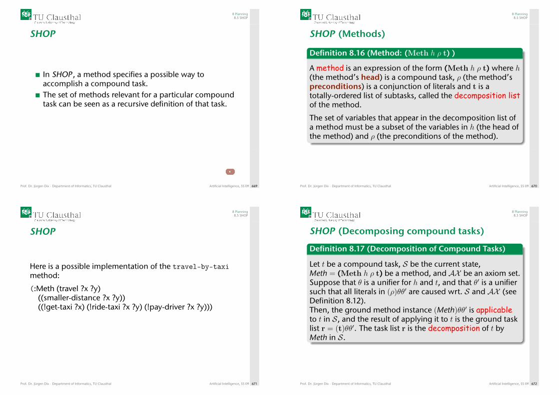
8 Planning8.5 SHOP
SHOP
In SHOP , a method specifies a possible way toaccomplish a compound task.The set of methods relevant for a particular compoundtask can be seen as a recursive definition of that task.
Prof. Dr. Jürgen Dix · Department of Informatics, TU Clausthal Artificial Intelligence, SS 09 669
8 Planning8.5 SHOP
SHOP (Methods)
Definition 8.16 (Method: (Meth h ρ t) )
A method is an expression of the form (Meth h ρ t) where h(the method’s head) is a compound task, ρ (the method’spreconditions) is a conjunction of literals and t is atotally-ordered list of subtasks, called the decomposition listof the method.
The set of variables that appear in the decomposition list ofa method must be a subset of the variables in h (the head ofthe method) and ρ (the preconditions of the method).
Prof. Dr. Jürgen Dix · Department of Informatics, TU Clausthal Artificial Intelligence, SS 09 670
8 Planning8.5 SHOP
SHOP
Here is a possible implementation of the travel-by-taximethod:
(:Meth (travel ?x ?y)((smaller-distance ?x ?y))((!get-taxi ?x) (!ride-taxi ?x ?y) (!pay-driver ?x ?y)))
Prof. Dr. Jürgen Dix · Department of Informatics, TU Clausthal Artificial Intelligence, SS 09 671
8 Planning8.5 SHOP
SHOP (Decomposing compound tasks)
Definition 8.17 (Decomposition of Compound Tasks)
Let t be a compound task, S be the current state,Meth = (Meth h ρ t) be a method, and AX be an axiom set.Suppose that θ is a unifier for h and t, and that θ′ is a unifiersuch that all literals in (ρ)θθ′ are caused wrt. S and AX (seeDefinition 8.12).Then, the ground method instance (Meth)θθ′ is applicableto t in S, and the result of applying it to t is the ground tasklist r = (t)θθ′. The task list r is the decomposition of t byMeth in S.
Prof. Dr. Jürgen Dix · Department of Informatics, TU Clausthal Artificial Intelligence, SS 09 672
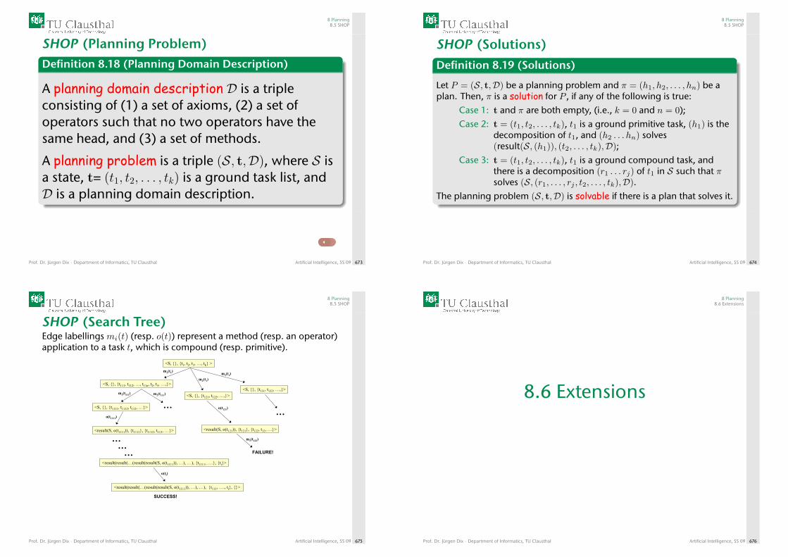
8 Planning8.5 SHOP
SHOP (Planning Problem)Definition 8.18 (Planning Domain Description)
A planning domain description D is a tripleconsisting of (1) a set of axioms, (2) a set ofoperators such that no two operators have thesame head, and (3) a set of methods.
A planning problem is a triple (S, t,D), where S isa state, t= (t1, t2, . . . , tk) is a ground task list, andD is a planning domain description.
Prof. Dr. Jürgen Dix · Department of Informatics, TU Clausthal Artificial Intelligence, SS 09 673
8 Planning8.5 SHOP
SHOP (Solutions)Definition 8.19 (Solutions)
Let P = (S, t,D) be a planning problem and π = (h1, h2, . . . , hn) be aplan. Then, π is a solution for P , if any of the following is true:
Case 1: t and π are both empty, (i.e., k = 0 and n = 0);Case 2: t = (t1, t2, . . . , tk), t1 is a ground primitive task, (h1) is the
decomposition of t1, and (h2 . . . hn) solves(result(S, (h1)), (t2, . . . , tk),D);
Case 3: t = (t1, t2, . . . , tk), t1 is a ground compound task, andthere is a decomposition (r1 . . . rj) of t1 in S such that πsolves (S, (r1, . . . , rj , t2, . . . , tk),D).
The planning problem (S, t,D) is solvable if there is a plan that solves it.
Prof. Dr. Jürgen Dix · Department of Informatics, TU Clausthal Artificial Intelligence, SS 09 674
8 Planning8.5 SHOP
SHOP (Search Tree)Edge labellings mi(t) (resp. o(t)) represent a method (resp. an operator)application to a task t, which is compound (resp. primitive).
<S, {}, {t1, t2, t3, …, tk} >m1(t1)
m2(t1)m3(t1)
<S, {}, {t111, t112, …, t11n, t2, t3, …,}>
<S, {}, {t121, t122, …,}><S, {}, {t131, t132, …,}>
…o(t121)
<result(S, o(t121)), {t121}, {t122, t12, …}>
m1(t122)
FAILURE!
m1(t111)
<S, {}, {t1111, t1112, t112, …}>
m2(t111)
…o(t1111)
<result(S, o(t1111)), {t1111}, {t1112, t112, …}>
………
<result(result(…(result(result(S, o(t1111)), …), …), {t1111, ….}, {ti}>
o(ti)
<result(result(…(result(result(S, o(t1111)), …), …), {t111, …., ti}, {}>
SUCCESS!
Prof. Dr. Jürgen Dix · Department of Informatics, TU Clausthal Artificial Intelligence, SS 09 675
8 Planning8.6 Extensions
8.6 Extensions
Prof. Dr. Jürgen Dix · Department of Informatics, TU Clausthal Artificial Intelligence, SS 09 676
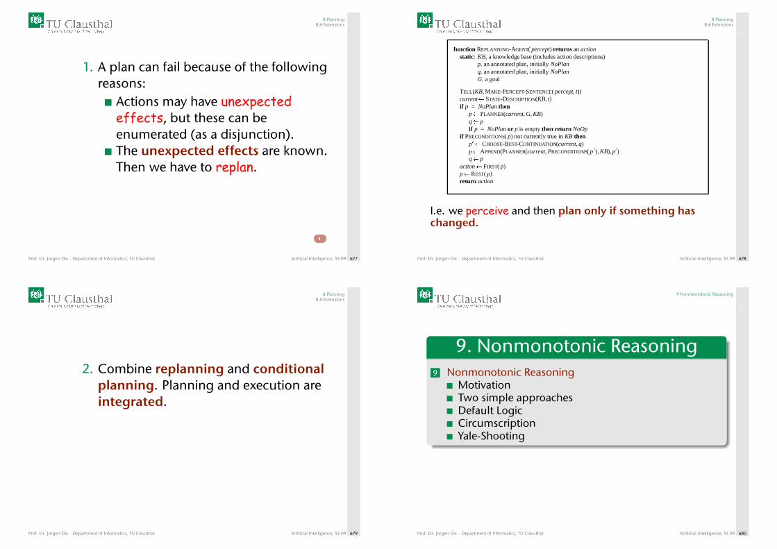
8 Planning8.6 Extensions
1. A plan can fail because of the followingreasons:
Actions may have unexpectedeffects, but these can beenumerated (as a disjunction).The unexpected effects are known.Then we have to replan.
Prof. Dr. Jürgen Dix · Department of Informatics, TU Clausthal Artificial Intelligence, SS 09 677
8 Planning8.6 Extensions
function REPLANNING-AGENT( percept) returns an actionstatic: KB, a knowledge base (includes action descriptions)
p, an annotated plan, initially NoPlanq, an annotated plan, initially NoPlanG, a goal
TELL(KB, MAKE-PERCEPT-SENTENCE( percept, t))current� STATE-DESCRIPTION(KB, t)if p = NoPlan then
p� PLANNER(current, G, KB)q� pif p = NoPlan or p is empty then return NoOp
if PRECONDITIONS( p) not currently true in KB thenp��CHOOSE-BEST-CONTINUATION(current, q)
p�APPEND(PLANNER(current, PRECONDITIONS( p �), KB), p�)q� p
action� FIRST( p)p�REST( p)return action
I.e. we perceive and then plan only if something haschanged.
Prof. Dr. Jürgen Dix · Department of Informatics, TU Clausthal Artificial Intelligence, SS 09 678
8 Planning8.6 Extensions
2. Combine replanning and conditionalplanning. Planning and execution areintegrated.
Prof. Dr. Jürgen Dix · Department of Informatics, TU Clausthal Artificial Intelligence, SS 09 679
9 Nonmonotonic Reasoning
9. Nonmonotonic Reasoning9 Nonmonotonic Reasoning
MotivationTwo simple approachesDefault LogicCircumscriptionYale-Shooting
Prof. Dr. Jürgen Dix · Department of Informatics, TU Clausthal Artificial Intelligence, SS 09 680
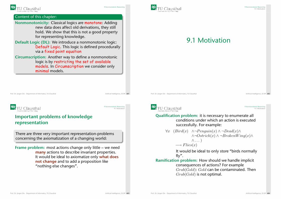
9 Nonmonotonic Reasoning
Content of this chapter:
Nonmonotonicity: Classical logics are monotone: Addingnew data does affect old derivations, they stillhold. We show that this is not a good propertyfor representing knowledge.
Default Logic (DL): We introduce a nonmonotonic logic:Default Logic. This logic is defined procedurallyvia a fixed point equation
Circumscription: Another way to define a nonmonotoniclogic is by restricting the set of availablemodels. In Circumscription we consider onlyminimal models.
Prof. Dr. Jürgen Dix · Department of Informatics, TU Clausthal Artificial Intelligence, SS 09 681
9 Nonmonotonic Reasoning9.1 Motivation
9.1 Motivation
Prof. Dr. Jürgen Dix · Department of Informatics, TU Clausthal Artificial Intelligence, SS 09 682
9 Nonmonotonic Reasoning9.1 Motivation
Important problems of knowledgerepresentation
There are three very important representation-problemsconcerning the axiomatization of a changing world:
Frame problem: most actions change only little – we needmany actions to describe invariant properties.It would be ideal to axiomatize only what doesnot change and to add a proposition like“nothing else changes”.
Prof. Dr. Jürgen Dix · Department of Informatics, TU Clausthal Artificial Intelligence, SS 09 683
9 Nonmonotonic Reasoning9.1 Motivation
Qualification problem: it is necessary to enumerate allconditions under which an action is executedsuccessfully. For example:
∀x (Bird(x) ∧¬Penguin(x) ∧ ¬Dead(x)∧∧¬Ostrich(x) ∧ ¬BrokenWing(x)∧∧ . . . )
−→ Flies(x)
It would be ideal to only store “birds normallyfly”.
Ramification problem: How should we handle implicitconsequences of actions? For exampleGrab(Gold): Gold can be contaminated. ThenGrab(Gold) is not optimal.
Prof. Dr. Jürgen Dix · Department of Informatics, TU Clausthal Artificial Intelligence, SS 09 684

9 Nonmonotonic Reasoning9.1 Motivation
Klassische Logiken lassen sich üblicherweise durch dieAngabe zweier Dinge spezifizieren:
1 einer Menge von Axiomen und2 einer Menge von Schlußregeln.
Formal geschieht dies durch eine Folgerungsrelation`⊆ 2Fml × Fml:
Φ ` ψ bedeutet “aus Φ ist ψ ableitbar”.
Siehe Definition 4.11.
Prof. Dr. Jürgen Dix · Department of Informatics, TU Clausthal Artificial Intelligence, SS 09 685
9 Nonmonotonic Reasoning9.1 Motivation
Warum Nichtmonotonie?1 Datenbanken2 Faustregeln3 Erklärungen
Prof. Dr. Jürgen Dix · Department of Informatics, TU Clausthal Artificial Intelligence, SS 09 686
9 Nonmonotonic Reasoning9.1 Motivation
DatenbankenEine DB enthält nur positive Fakten (Liste von verfügbarenFlügen). Klassisch gesehen ist daraus keine negativeInformation ableitbar.Aber man möchte, daß aus
flug(M,B, 9.00), f lug(M,B, 12.00),f lug(M,B, 15.00), f lug(M,B, 18.00),
auch¬flug(M,B, 11.00)
folgt.Die klassische Logik ist zu schwach, um solcheAbleitungen zu erlauben: Wir können wederflug(M,B, 11.00) noch ¬flug(M,B, 11.00) ableiten.
Prof. Dr. Jürgen Dix · Department of Informatics, TU Clausthal Artificial Intelligence, SS 09 687
9 Nonmonotonic Reasoning9.1 Motivation
Faustregeln
Sachverhalte sind oft nicht genügend spezifiziert, dagewisse Hintergrundinformationen nötig sind:
“Die Liste ist vollständig.”
Anstatt streng logischer Schlüsse benutzen Menschen eherFaustregeln (engl. Defaults).
Prof. Dr. Jürgen Dix · Department of Informatics, TU Clausthal Artificial Intelligence, SS 09 688

9 Nonmonotonic Reasoning9.1 Motivation
Example 9.1 (Tweety und Fred)
Betrachten wir die folgenden beiden Faustregeln:1 vogel(x) |||∼ fliegt(x): Normalerweise können Vögel
fliegen,2 pinguin(x) |||∼ ¬fliegt(x): Normalerweise können
Pinguine nicht fliegen.Angenommen, wir wissen auch noch, daß Pinguine Vögelsind und daß sowohl tweety als auch fred zweibestimmte Vögel sind.Daraus sollte folgen, daß sowohl tweety als auch fredfliegen können.
Prof. Dr. Jürgen Dix · Department of Informatics, TU Clausthal Artificial Intelligence, SS 09 689
9 Nonmonotonic Reasoning9.1 Motivation
Wie geht das in klassischer Logik?Betrachten wir die Theorie
∀x(vogel(x)→ fliegt(x))∀x(pinguin(x)→ ¬fliegt(x)),
zusammen mit den Fakten vogel(tweety), vogel(fred) und∀x(pinguin(x)→ vogel(x)).Nun erfahren wir, daß fred ein Pinguin ist. Addieren wirpinguin(fred) zu unserer Formelmenge, können wirplötzlich alles mögliche ableiten:
fliegt(fred),¬fliegt(fred),
— unsere Formelmenge ist also inkonsistent: Jede Formel istableitbar.
Prof. Dr. Jürgen Dix · Department of Informatics, TU Clausthal Artificial Intelligence, SS 09 690
9 Nonmonotonic Reasoning9.1 Motivation
Man könnte aber auch wie folgt vorgehen:
∀x((vogel(x) ∧ ¬pinguin(x))→ fliegt(x)),∀x(pinguin(x)→ ¬fliegt(x)).
Dann hätte man zwar die Inkonsistenz vermieden, aberman kann nicht mehr
fliegt(tweety)
ableiten, da es keine Möglichkeit gibt, ¬pinguin(tweety)abzuleiten.
Prof. Dr. Jürgen Dix · Department of Informatics, TU Clausthal Artificial Intelligence, SS 09 691
9 Nonmonotonic Reasoning9.1 Motivation
Wir möchten gerne folgendes:
1 Φ |||∼ fliegt(fred) und2 Φ ∪ {pinguin(fred)} |||∼ ¬fliegt(fred).
In jeder monotonen Logik ist im zweiten Fall fliegt(fred)immer noch ableitbar und daher ergibt sich zwangsläufigeine Inkonsistenz.
Prof. Dr. Jürgen Dix · Department of Informatics, TU Clausthal Artificial Intelligence, SS 09 692

9 Nonmonotonic Reasoning9.1 Motivation
ErklärungenErklärungen
Wir wissen, daß meistens der Rasen dann naß wird, wenn esregnet. Er wird aber auch naß, wenn der Rasensprenger anist (und dann bleibt die Straße trocken).
Damit ergeben sich verschiedene Erklärungen, je nachWissensstand:
Der Rasen ist naß.Erklärung: Es hat geregnet.Aber die Straße ist trocken.Revidierte Erklärung: Der Rasensprenger war an.
Dieses Example führt zum Prinzip der Abduktion:
Wenn ψ und φ→ ψ, dann schließen wir auf φ.
Prof. Dr. Jürgen Dix · Department of Informatics, TU Clausthal Artificial Intelligence, SS 09 693
9 Nonmonotonic Reasoning9.1 Motivation
Beispiele für nichtmonotone Phänomene
Example 9.2 (Ausnahmen)
Folgende Fakten sind bekannt:1 Vögel fliegen normalerweise.2 Ausnahmen sind Pinguine, sie fliegen nicht.3 Tweety ist ein Vogel.
Intuitiv möchten wir natürlich ableiten, daß Tweety fliegt.Nach einiger Zeit lernen wir aber: Tweety ist ein Pinguin.Fliegt Tweety immer noch?Intuitiv erwarten wir: Nein.
Prof. Dr. Jürgen Dix · Department of Informatics, TU Clausthal Artificial Intelligence, SS 09 694
9 Nonmonotonic Reasoning9.1 Motivation
Example 9.3 (Nixon-Diamant)
Folgende Fakten sind bekannt:1 Quäker sind normalerweise Pazifisten.2 Republikaner sind normalerweise keine Pazifisten.3 Nixon war sowohl Quäker als auch Republikaner.
War Nixon ein Pazifist?Wir erwarten hier, daß wir keine eindeutige Aussage treffenkönnen.
Prof. Dr. Jürgen Dix · Department of Informatics, TU Clausthal Artificial Intelligence, SS 09 695
9 Nonmonotonic Reasoning9.1 Motivation
Example 9.4 (Disjunktion)
Wir haben zwei Defaults und ein Faktum.1 Normalerweise trinken Italiener gerne Wein, Franzosen
auch.2 Georg ist Franzose oder Italiener.
Trinkt Georg gerne Wein?Hier erwarten wir die Antwort Ja.
Prof. Dr. Jürgen Dix · Department of Informatics, TU Clausthal Artificial Intelligence, SS 09 696
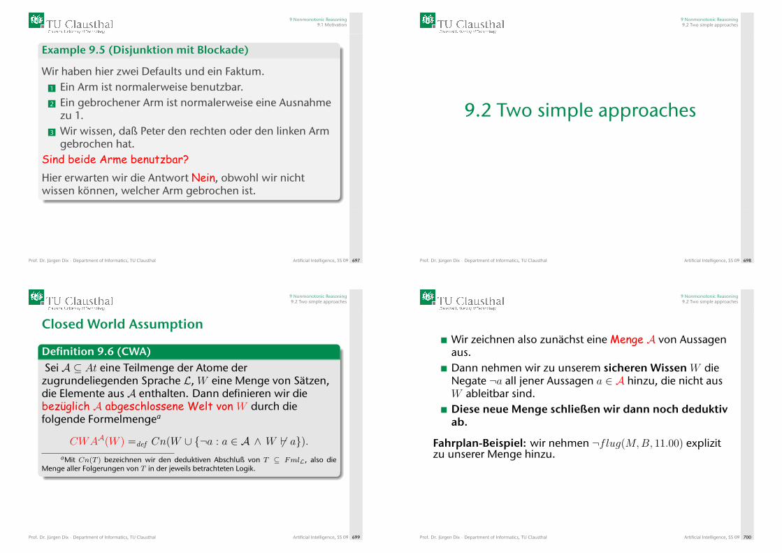
9 Nonmonotonic Reasoning9.1 Motivation
Example 9.5 (Disjunktion mit Blockade)
Wir haben hier zwei Defaults und ein Faktum.1 Ein Arm ist normalerweise benutzbar.2 Ein gebrochener Arm ist normalerweise eine Ausnahme
zu 1.3 Wir wissen, daß Peter den rechten oder den linken Arm
gebrochen hat.Sind beide Arme benutzbar?Hier erwarten wir die Antwort Nein, obwohl wir nichtwissen können, welcher Arm gebrochen ist.
Prof. Dr. Jürgen Dix · Department of Informatics, TU Clausthal Artificial Intelligence, SS 09 697
9 Nonmonotonic Reasoning9.2 Two simple approaches
9.2 Two simple approaches
Prof. Dr. Jürgen Dix · Department of Informatics, TU Clausthal Artificial Intelligence, SS 09 698
9 Nonmonotonic Reasoning9.2 Two simple approaches
Closed World Assumption
Definition 9.6 (CWA)Sei A ⊆ At eine Teilmenge der Atome derzugrundeliegenden Sprache L, W eine Menge von Sätzen,die Elemente aus A enthalten. Dann definieren wir diebezüglich A abgeschlossene Welt von W durch diefolgende Formelmengea
CWAA(W ) =def Cn(W ∪ {¬a : a ∈ A ∧ W 6` a}).aMit Cn(T ) bezeichnen wir den deduktiven Abschluß von T ⊆ FmlL, also die
Menge aller Folgerungen von T in der jeweils betrachteten Logik.
Prof. Dr. Jürgen Dix · Department of Informatics, TU Clausthal Artificial Intelligence, SS 09 699
9 Nonmonotonic Reasoning9.2 Two simple approaches
Wir zeichnen also zunächst eine Menge A von Aussagenaus.Dann nehmen wir zu unserem sicheren Wissen W dieNegate ¬a all jener Aussagen a ∈ A hinzu, die nicht ausW ableitbar sind.Diese neue Menge schließen wir dann noch deduktivab.
Fahrplan-Beispiel: wir nehmen ¬flug(M,B, 11.00) explizitzu unserer Menge hinzu.
Prof. Dr. Jürgen Dix · Department of Informatics, TU Clausthal Artificial Intelligence, SS 09 700
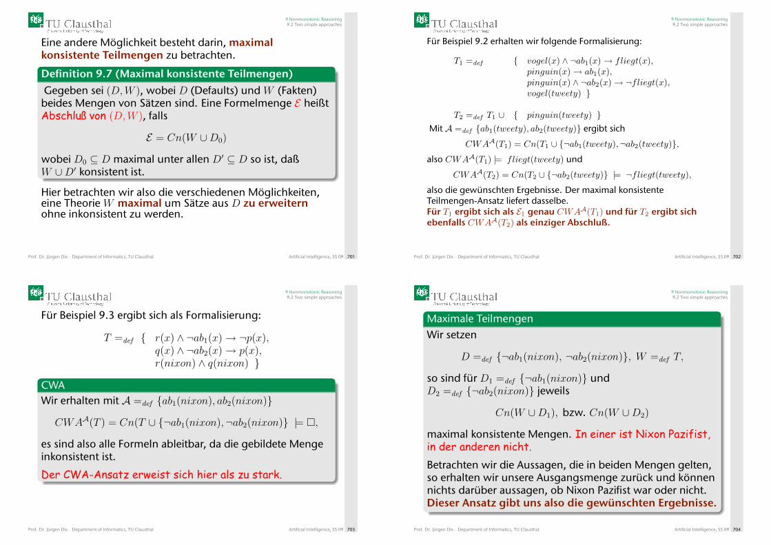
9 Nonmonotonic Reasoning9.2 Two simple approaches
Eine andere Möglichkeit besteht darin, maximalkonsistente Teilmengen zu betrachten.
Definition 9.7 (Maximal konsistente Teilmengen)
Gegeben sei (D,W ), wobei D (Defaults) und W (Fakten)beides Mengen von Sätzen sind. Eine Formelmenge E heißtAbschluß von (D,W ), falls
E = Cn(W ∪D0)
wobei D0 ⊆ D maximal unter allen D′ ⊆ D so ist, daßW ∪D′ konsistent ist.
Hier betrachten wir also die verschiedenen Möglichkeiten,eine Theorie W maximal um Sätze aus D zu erweiternohne inkonsistent zu werden.
Prof. Dr. Jürgen Dix · Department of Informatics, TU Clausthal Artificial Intelligence, SS 09 701
9 Nonmonotonic Reasoning9.2 Two simple approaches
Für Beispiel 9.2 erhalten wir folgende Formalisierung:
T1 =def { vogel(x) ∧ ¬ab1(x)→ fliegt(x),pinguin(x)→ ab1(x),pinguin(x) ∧ ¬ab2(x)→ ¬fliegt(x),vogel(tweety) }
T2 =def T1 ∪ { pinguin(tweety) }Mit A =def {ab1(tweety), ab2(tweety)} ergibt sich
CWAA(T1) = Cn(T1 ∪ {¬ab1(tweety),¬ab2(tweety)},also CWAA(T1) |= fliegt(tweety) und
CWAA(T2) = Cn(T2 ∪ {¬ab2(tweety)} |= ¬fliegt(tweety),
also die gewünschten Ergebnisse. Der maximal konsistenteTeilmengen-Ansatz liefert dasselbe.Für T1 ergibt sich als E1 genau CWAA(T1) und für T2 ergibt sichebenfalls CWAA(T2) als einziger Abschluß.
Prof. Dr. Jürgen Dix · Department of Informatics, TU Clausthal Artificial Intelligence, SS 09 702
9 Nonmonotonic Reasoning9.2 Two simple approaches
Für Beispiel 9.3 ergibt sich als Formalisierung:
T =def { r(x) ∧ ¬ab1(x)→ ¬p(x),q(x) ∧ ¬ab2(x)→ p(x),r(nixon) ∧ q(nixon) }
CWAWir erhalten mit A =def {ab1(nixon), ab2(nixon)}
CWAA(T ) = Cn(T ∪ {¬ab1(nixon),¬ab2(nixon)} |= �,
es sind also alle Formeln ableitbar, da die gebildete Mengeinkonsistent ist.
Der CWA-Ansatz erweist sich hier als zu stark.
Prof. Dr. Jürgen Dix · Department of Informatics, TU Clausthal Artificial Intelligence, SS 09 703
9 Nonmonotonic Reasoning9.2 Two simple approaches
Maximale TeilmengenWir setzen
D =def {¬ab1(nixon), ¬ab2(nixon)}, W =def T,
so sind für D1 =def {¬ab1(nixon)} undD2 =def {¬ab2(nixon)} jeweils
Cn(W ∪D1), bzw. Cn(W ∪D2)
maximal konsistente Mengen. In einer ist Nixon Pazifist,in der anderen nicht.Betrachten wir die Aussagen, die in beiden Mengen gelten,so erhalten wir unsere Ausgangsmenge zurück und könnennichts darüber aussagen, ob Nixon Pazifist war oder nicht.Dieser Ansatz gibt uns also die gewünschten Ergebnisse.
Prof. Dr. Jürgen Dix · Department of Informatics, TU Clausthal Artificial Intelligence, SS 09 704
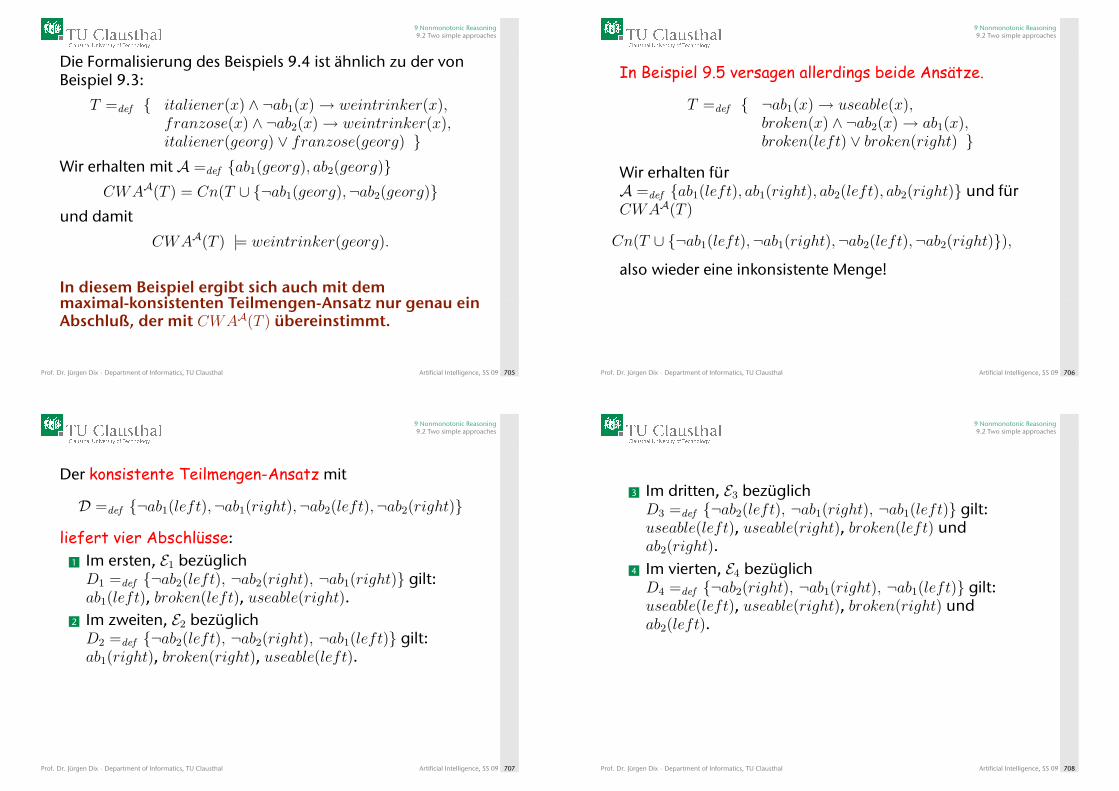
9 Nonmonotonic Reasoning9.2 Two simple approaches
Die Formalisierung des Beispiels 9.4 ist ähnlich zu der vonBeispiel 9.3:
T =def { italiener(x) ∧ ¬ab1(x)→ weintrinker(x),franzose(x) ∧ ¬ab2(x)→ weintrinker(x),italiener(georg) ∨ franzose(georg) }
Wir erhalten mit A =def {ab1(georg), ab2(georg)}CWAA(T ) = Cn(T ∪ {¬ab1(georg),¬ab2(georg)}
und damit
CWAA(T ) |= weintrinker(georg).
In diesem Beispiel ergibt sich auch mit demmaximal-konsistenten Teilmengen-Ansatz nur genau einAbschluß, der mit CWAA(T ) übereinstimmt.
Prof. Dr. Jürgen Dix · Department of Informatics, TU Clausthal Artificial Intelligence, SS 09 705
9 Nonmonotonic Reasoning9.2 Two simple approaches
In Beispiel 9.5 versagen allerdings beide Ansätze.
T =def { ¬ab1(x)→ useable(x),broken(x) ∧ ¬ab2(x)→ ab1(x),broken(left) ∨ broken(right) }
Wir erhalten fürA =def {ab1(left), ab1(right), ab2(left), ab2(right)} und fürCWAA(T )
Cn(T ∪ {¬ab1(left),¬ab1(right),¬ab2(left),¬ab2(right)}),
also wieder eine inkonsistente Menge!
Prof. Dr. Jürgen Dix · Department of Informatics, TU Clausthal Artificial Intelligence, SS 09 706
9 Nonmonotonic Reasoning9.2 Two simple approaches
Der konsistente Teilmengen-Ansatz mit
D =def {¬ab1(left),¬ab1(right),¬ab2(left),¬ab2(right)}
liefert vier Abschlüsse:1 Im ersten, E1 bezüglichD1 =def {¬ab2(left), ¬ab2(right), ¬ab1(right)} gilt:ab1(left), broken(left), useable(right).
2 Im zweiten, E2 bezüglichD2 =def {¬ab2(left), ¬ab2(right), ¬ab1(left)} gilt:ab1(right), broken(right), useable(left).
Prof. Dr. Jürgen Dix · Department of Informatics, TU Clausthal Artificial Intelligence, SS 09 707
9 Nonmonotonic Reasoning9.2 Two simple approaches
3 Im dritten, E3 bezüglichD3 =def {¬ab2(left), ¬ab1(right), ¬ab1(left)} gilt:useable(left), useable(right), broken(left) undab2(right).
4 Im vierten, E4 bezüglichD4 =def {¬ab2(right), ¬ab1(right), ¬ab1(left)} gilt:useable(left), useable(right), broken(right) undab2(left).
Prof. Dr. Jürgen Dix · Department of Informatics, TU Clausthal Artificial Intelligence, SS 09 708
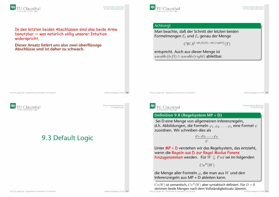
9 Nonmonotonic Reasoning9.2 Two simple approaches
In den letzten beiden Abschlüssen sind also beide Armebenutzbar — was natürlich völlig unserer Intuitionwiderspricht.Dieser Ansatz liefert uns also zwei überflüssigeAbschlüsse und ist daher zu schwach.
Prof. Dr. Jürgen Dix · Department of Informatics, TU Clausthal Artificial Intelligence, SS 09 709
9 Nonmonotonic Reasoning9.2 Two simple approaches
Achtung!
Man beachte, daß der Schnitt der letzten beidenFormelmengen E3 und E4 genau der Menge
CWA{¬ab1(left),¬ab1(right)}(T )
entspricht. Auch aus dieser Menge istuseable(left) ∧ useable(right) ableitbar.
Prof. Dr. Jürgen Dix · Department of Informatics, TU Clausthal Artificial Intelligence, SS 09 710
9 Nonmonotonic Reasoning9.3 Default Logic
9.3 Default Logic
Prof. Dr. Jürgen Dix · Department of Informatics, TU Clausthal Artificial Intelligence, SS 09 711
9 Nonmonotonic Reasoning9.3 Default Logic
Definition 9.8 (Regelsystem MP + D)Sei D eine Menge von allgemeinen Inferenzregeln,d.h. Abbildungen, die Formeln ϕ1, ϕ2, . . . , ϕn eine Formel ψzuordnen. Wir schreiben dies als
ϕ1, ϕ2, . . . , ϕnψ
.
Unter MP + D verstehen wir das Regelsystem, das entsteht,wenn die Regeln aus D zur Regel Modus Ponenshinzugenommen werden. Für W ⊆ Fml sei im folgenden
CnD(W )
die Menge aller Formeln ϕ, die man aus W und denInferenzregeln aus MP + D ableiten kann.
Cn(W ) ist semantisch, CnD(W ) aber syntaktisch definiert. Für D = ∅stimmen beide Mengen nach dem Vollständigkeitssatz überein.
Prof. Dr. Jürgen Dix · Department of Informatics, TU Clausthal Artificial Intelligence, SS 09 712
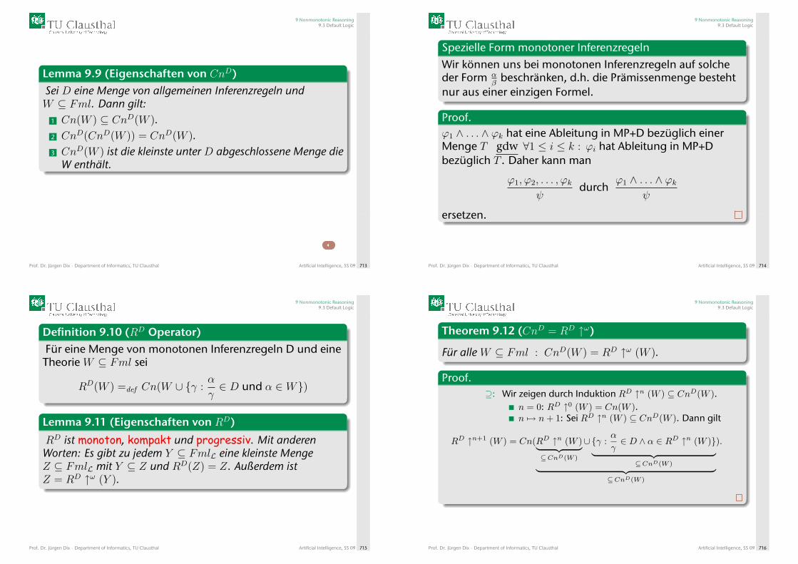
9 Nonmonotonic Reasoning9.3 Default Logic
Lemma 9.9 (Eigenschaften von CnD)Sei D eine Menge von allgemeinen Inferenzregeln undW ⊆ Fml. Dann gilt:
1 Cn(W ) ⊆ CnD(W ).2 CnD(CnD(W )) = CnD(W ).3 CnD(W ) ist die kleinste unter D abgeschlossene Menge die
W enthält.
Prof. Dr. Jürgen Dix · Department of Informatics, TU Clausthal Artificial Intelligence, SS 09 713
9 Nonmonotonic Reasoning9.3 Default Logic
Spezielle Form monotoner Inferenzregeln
Wir können uns bei monotonen Inferenzregeln auf solcheder Form α
βbeschränken, d.h. die Prämissenmenge besteht
nur aus einer einzigen Formel.
Proof.ϕ1 ∧ . . . ∧ ϕk hat eine Ableitung in MP+D bezüglich einerMenge T gdw ∀1 ≤ i ≤ k : ϕi hat Ableitung in MP+Dbezüglich T . Daher kann man
ϕ1, ϕ2, . . . , ϕkψ
durchϕ1 ∧ . . . ∧ ϕk
ψ
ersetzen.
Prof. Dr. Jürgen Dix · Department of Informatics, TU Clausthal Artificial Intelligence, SS 09 714
9 Nonmonotonic Reasoning9.3 Default Logic
Definition 9.10 (RD Operator)Für eine Menge von monotonen Inferenzregeln D und eineTheorie W ⊆ Fml sei
RD(W ) =def Cn(W ∪ {γ :α
γ∈ D und α ∈ W})
Lemma 9.11 (Eigenschaften von RD)
RD ist monoton, kompakt und progressiv. Mit anderenWorten: Es gibt zu jedem Y ⊆ FmlL eine kleinste MengeZ ⊆ FmlL mit Y ⊆ Z und RD(Z) = Z. Außerdem istZ = RD ↑ω (Y ).
Prof. Dr. Jürgen Dix · Department of Informatics, TU Clausthal Artificial Intelligence, SS 09 715
9 Nonmonotonic Reasoning9.3 Default Logic
Theorem 9.12 (CnD = RD ↑ω)
Für alle W ⊆ Fml : CnD(W ) = RD ↑ω (W ).
Proof.⊇: Wir zeigen durch Induktion RD ↑n (W ) ⊆ CnD(W ).
n = 0: RD ↑0 (W ) = Cn(W ).n 7→ n+ 1: Sei RD ↑n (W ) ⊆ CnD(W ). Dann gilt
RD ↑n+1 (W ) = Cn(RD ↑n (W )︸ ︷︷ ︸⊆CnD(W )
∪{γ :α
γ∈ D ∧ α ∈ RD ↑n (W )}︸ ︷︷ ︸⊆CnD(W )︸ ︷︷ ︸
⊆CnD(W )
).
Prof. Dr. Jürgen Dix · Department of Informatics, TU Clausthal Artificial Intelligence, SS 09 716
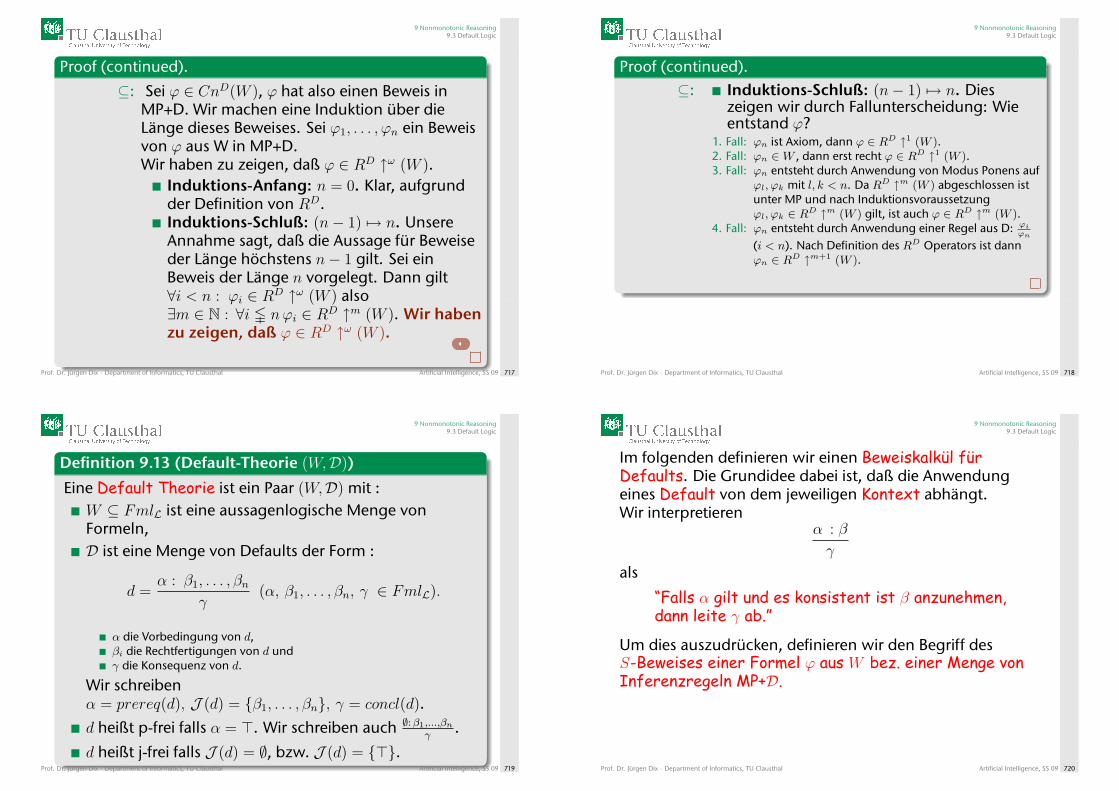
9 Nonmonotonic Reasoning9.3 Default Logic
Proof (continued).
⊆: Sei ϕ ∈ CnD(W ), ϕ hat also einen Beweis inMP+D. Wir machen eine Induktion über dieLänge dieses Beweises. Sei ϕ1, . . . , ϕn ein Beweisvon ϕ aus W in MP+D.Wir haben zu zeigen, daß ϕ ∈ RD ↑ω (W ).
Induktions-Anfang: n = 0. Klar, aufgrundder Definition von RD.Induktions-Schluß: (n− 1) 7→ n. UnsereAnnahme sagt, daß die Aussage für Beweiseder Länge höchstens n− 1 gilt. Sei einBeweis der Länge n vorgelegt. Dann gilt∀i < n : ϕi ∈ RD ↑ω (W ) also∃m ∈ N : ∀i � nϕi ∈ RD ↑m (W ). Wir habenzu zeigen, daß ϕ ∈ RD ↑ω (W ).
Prof. Dr. Jürgen Dix · Department of Informatics, TU Clausthal Artificial Intelligence, SS 09 717
9 Nonmonotonic Reasoning9.3 Default Logic
Proof (continued).⊆: Induktions-Schluß: (n− 1) 7→ n. Dies
zeigen wir durch Fallunterscheidung: Wieentstand ϕ?
1. Fall: ϕn ist Axiom, dann ϕ ∈ RD ↑1 (W ).2. Fall: ϕn ∈W , dann erst recht ϕ ∈ RD ↑1 (W ).3. Fall: ϕn entsteht durch Anwendung von Modus Ponens auf
ϕl, ϕk mit l, k < n. Da RD ↑m (W ) abgeschlossen istunter MP und nach Induktionsvoraussetzungϕl, ϕk ∈ RD ↑m (W ) gilt, ist auch ϕ ∈ RD ↑m (W ).
4. Fall: ϕn entsteht durch Anwendung einer Regel aus D: ϕiϕn
(i < n). Nach Definition des RD Operators ist dannϕn ∈ RD ↑m+1 (W ).
Prof. Dr. Jürgen Dix · Department of Informatics, TU Clausthal Artificial Intelligence, SS 09 718
9 Nonmonotonic Reasoning9.3 Default Logic
Definition 9.13 (Default-Theorie (W,D))
Eine Default Theorie ist ein Paar (W,D) mit :W ⊆ FmlL ist eine aussagenlogische Menge vonFormeln,D ist eine Menge von Defaults der Form :
d =α : β1, . . . , βn
γ(α, β1, . . . , βn, γ ∈ FmlL).
α die Vorbedingung von d,βi die Rechtfertigungen von d undγ die Konsequenz von d.
Wir schreibenα = prereq(d), J (d) = {β1, . . . , βn}, γ = concl(d).
d heißt p-frei falls α = >. Wir schreiben auch ∅:β1,...,βnγ
.
d heißt j-frei falls J (d) = ∅, bzw. J (d) = {>}.Prof. Dr. Jürgen Dix · Department of Informatics, TU Clausthal Artificial Intelligence, SS 09 719
9 Nonmonotonic Reasoning9.3 Default Logic
Im folgenden definieren wir einen Beweiskalkül fürDefaults. Die Grundidee dabei ist, daß die Anwendungeines Default von dem jeweiligen Kontext abhängt.Wir interpretieren
α : β
γ
als
“Falls α gilt und es konsistent ist β anzunehmen,dann leite γ ab.”
Um dies auszudrücken, definieren wir den Begriff desS-Beweises einer Formel ϕ aus W bez. einer Menge vonInferenzregeln MP+D.
Prof. Dr. Jürgen Dix · Department of Informatics, TU Clausthal Artificial Intelligence, SS 09 720
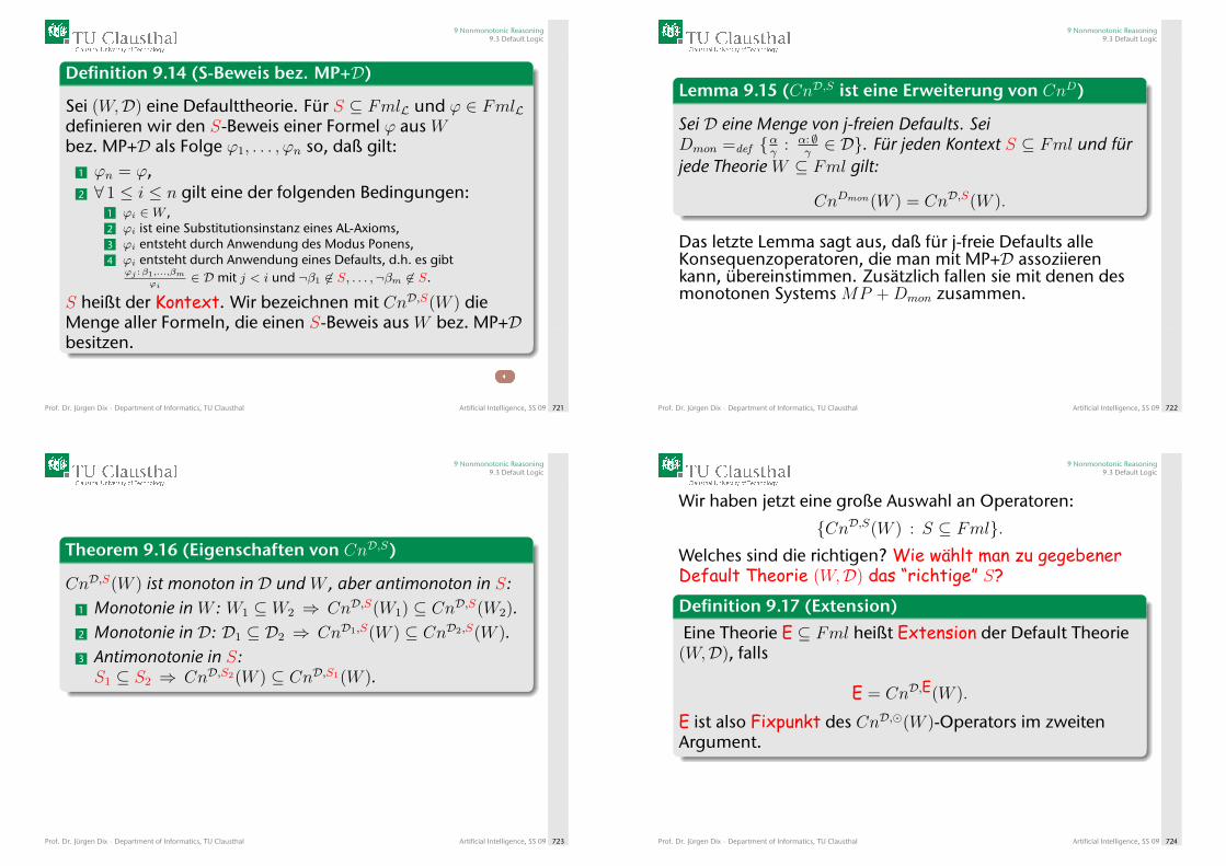
9 Nonmonotonic Reasoning9.3 Default Logic
Definition 9.14 (S-Beweis bez. MP+D)
Sei (W,D) eine Defaulttheorie. Für S ⊆ FmlL und ϕ ∈ FmlLdefinieren wir den S-Beweis einer Formel ϕ aus Wbez. MP+D als Folge ϕ1, . . . , ϕn so, daß gilt:
1 ϕn = ϕ,2 ∀ 1 ≤ i ≤ n gilt eine der folgenden Bedingungen:
1 ϕi ∈W ,2 ϕi ist eine Substitutionsinstanz eines AL-Axioms,3 ϕi entsteht durch Anwendung des Modus Ponens,4 ϕi entsteht durch Anwendung eines Defaults, d.h. es gibt
ϕj : β1,...,βm
ϕi∈ D mit j < i und ¬β1 6∈ S, . . . ,¬βm 6∈ S.
S heißt der Kontext. Wir bezeichnen mit CnD,S(W ) dieMenge aller Formeln, die einen S-Beweis aus W bez. MP+Dbesitzen.
Prof. Dr. Jürgen Dix · Department of Informatics, TU Clausthal Artificial Intelligence, SS 09 721
9 Nonmonotonic Reasoning9.3 Default Logic
Lemma 9.15 (CnD,S ist eine Erweiterung von CnD)
Sei D eine Menge von j-freien Defaults. SeiDmon =def {αγ : α: ∅
γ∈ D}. Für jeden Kontext S ⊆ Fml und für
jede Theorie W ⊆ Fml gilt:
CnDmon(W ) = CnD,S(W ).
Das letzte Lemma sagt aus, daß für j-freie Defaults alleKonsequenzoperatoren, die man mit MP+D assoziierenkann, übereinstimmen. Zusätzlich fallen sie mit denen desmonotonen Systems MP +Dmon zusammen.
Prof. Dr. Jürgen Dix · Department of Informatics, TU Clausthal Artificial Intelligence, SS 09 722
9 Nonmonotonic Reasoning9.3 Default Logic
Theorem 9.16 (Eigenschaften von CnD,S)
CnD,S(W ) ist monoton in D und W , aber antimonoton in S:1 Monotonie in W : W1 ⊆ W2 ⇒ CnD,S(W1) ⊆ CnD,S(W2).2 Monotonie in D: D1 ⊆ D2 ⇒ CnD1,S(W ) ⊆ CnD2,S(W ).3 Antimonotonie in S:S1 ⊆ S2 ⇒ CnD,S2(W ) ⊆ CnD,S1(W ).
Prof. Dr. Jürgen Dix · Department of Informatics, TU Clausthal Artificial Intelligence, SS 09 723
9 Nonmonotonic Reasoning9.3 Default Logic
Wir haben jetzt eine große Auswahl an Operatoren:
{CnD,S(W ) : S ⊆ Fml}.Welches sind die richtigen? Wie wählt man zu gegebenerDefault Theorie (W,D) das “richtige” S?
Definition 9.17 (Extension)
Eine Theorie E ⊆ Fml heißt Extension der Default Theorie(W,D), falls
E = CnD,E(W ).
E ist also Fixpunkt des CnD,�(W )-Operators im zweitenArgument.
Prof. Dr. Jürgen Dix · Department of Informatics, TU Clausthal Artificial Intelligence, SS 09 724
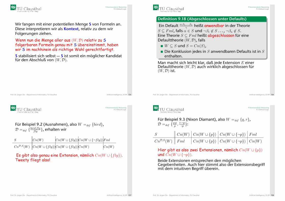
9 Nonmonotonic Reasoning9.3 Default Logic
Wir fangen mit einer potentiellen Menge S von Formeln an.Diese interpretieren wir als Kontext, relativ zu dem wirFolgerungen ziehen.
Wenn nun die Menge aller aus (W,D) relativ zu Sfolgerbaren Formeln genau mit S übereinstimmt, habenwir S im nachhinein als richtige Wahl gerechtfertigt.S stabilisiert sich selbst — S ist somit ein möglicher Kandidatfür den Abschluß von (W,D).
Prof. Dr. Jürgen Dix · Department of Informatics, TU Clausthal Artificial Intelligence, SS 09 725
9 Nonmonotonic Reasoning9.3 Default Logic
Definition 9.18 (Abgeschlossen unter Defaults)
Ein Default α:β1,...,βnγ
heißt anwendbar in der TheorieS ⊆ Fml, falls α ∈ S und ¬β1 6∈ S . . . , ¬βn 6∈ S.Eine Theorie S ⊆ Fml heißt abgeschlossen für eineDefaulttheorie (W,D), falls
W ⊆ S und S = Cn(S),Die Konklusion jedes in S anwendbaren Defaults ist in Senthalten.
Man macht sich leicht klar, daß jede Extension E einerDefaulttheorie (W,D) auch wirklich abgeschlossen für(W,D) ist.
Prof. Dr. Jürgen Dix · Department of Informatics, TU Clausthal Artificial Intelligence, SS 09 726
9 Nonmonotonic Reasoning9.3 Default Logic
Für Beispiel 9.2 (Ausnahmen), also W =def {bird},D =def { bird:fly
fly}, erhalten wir
S Cn(W ) Cn(W ∪ {fly})Cn(W ∪ {¬fly})Fml
CnD,S(W ) Cn(W ∪ {fly})Cn(W ∪ {fly})Cn(W ) Cn(W )
Es gibt also genau eine Extension, nämlich Cn(W ∪ {fly}).Tweety fliegt also!
Prof. Dr. Jürgen Dix · Department of Informatics, TU Clausthal Artificial Intelligence, SS 09 727
9 Nonmonotonic Reasoning9.3 Default Logic
Für Beispiel 9.3 (Nixon Diamant), also W =def {q, r},D =def { q:pp ,
r:¬p¬p }:
S Cn(W ) Cn(W ∪ {p}) Cn(W ∪ {¬p}) Fml
CnD,S(W ) Fml Cn(W ∪ {p}) Cn(W ∪ {¬p}) Cn(W )
Hier gibt es also zwei Extensionen, nämlich Cn(W ∪ {p})und Cn(W ∪ {¬p}).Beide Extensionen entsprechen den möglichenGegebenheiten. Auch hier stimmt also der Extensionsbegriffmit dem intuitiven Begriff überein.
Prof. Dr. Jürgen Dix · Department of Informatics, TU Clausthal Artificial Intelligence, SS 09 728
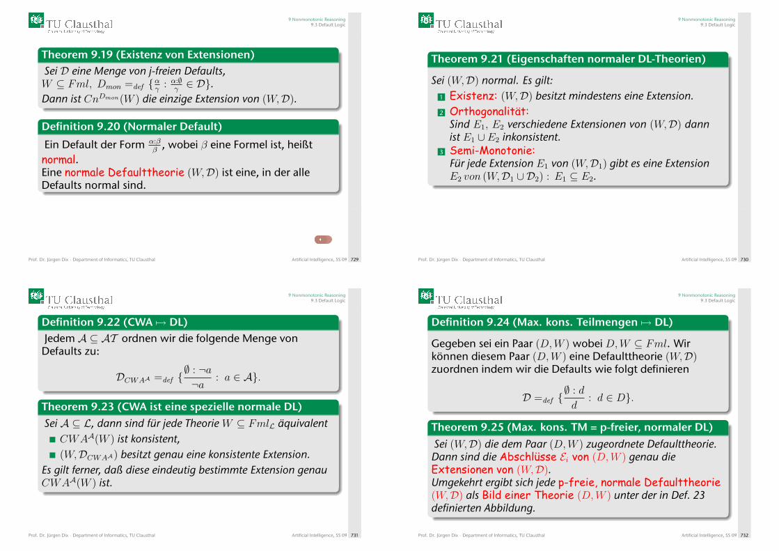
9 Nonmonotonic Reasoning9.3 Default Logic
Theorem 9.19 (Existenz von Extensionen)Sei D eine Menge von j-freien Defaults,W ⊆ Fml, Dmon =def {αγ : α:∅
γ∈ D}.
Dann ist CnDmon(W ) die einzige Extension von (W,D).
Definition 9.20 (Normaler Default)
Ein Default der Form α:ββ
, wobei β eine Formel ist, heißtnormal.Eine normale Defaulttheorie (W,D) ist eine, in der alleDefaults normal sind.
Prof. Dr. Jürgen Dix · Department of Informatics, TU Clausthal Artificial Intelligence, SS 09 729
9 Nonmonotonic Reasoning9.3 Default Logic
Theorem 9.21 (Eigenschaften normaler DL-Theorien)
Sei (W,D) normal. Es gilt:1 Existenz: (W,D) besitzt mindestens eine Extension.2 Orthogonalität:
Sind E1, E2 verschiedene Extensionen von (W,D) dannist E1 ∪ E2 inkonsistent.
3 Semi-Monotonie:Für jede Extension E1 von (W,D1) gibt es eine ExtensionE2 von (W,D1 ∪ D2) : E1 ⊆ E2.
Prof. Dr. Jürgen Dix · Department of Informatics, TU Clausthal Artificial Intelligence, SS 09 730
9 Nonmonotonic Reasoning9.3 Default Logic
Definition 9.22 (CWA 7→ DL)Jedem A ⊆ AT ordnen wir die folgende Menge vonDefaults zu:
DCWAA =def {∅ : ¬a¬a
: a ∈ A}.
Theorem 9.23 (CWA ist eine spezielle normale DL)Sei A ⊆ L, dann sind für jede Theorie W ⊆ FmlL äquivalent
CWAA(W ) ist konsistent,(W,DCWAA) besitzt genau eine konsistente Extension.
Es gilt ferner, daß diese eindeutig bestimmte Extension genauCWAA(W ) ist.
Prof. Dr. Jürgen Dix · Department of Informatics, TU Clausthal Artificial Intelligence, SS 09 731
9 Nonmonotonic Reasoning9.3 Default Logic
Definition 9.24 (Max. kons. Teilmengen 7→ DL)
Gegeben sei ein Paar (D,W ) wobei D,W ⊆ Fml. Wirkönnen diesem Paar (D,W ) eine Defaulttheorie (W,D)zuordnen indem wir die Defaults wie folgt definieren
D =def {∅ : d
d: d ∈ D}.
Theorem 9.25 (Max. kons. TM = p-freier, normaler DL)
Sei (W,D) die dem Paar (D,W ) zugeordnete Defaulttheorie.Dann sind die Abschlüsse Ei von (D,W ) genau dieExtensionen von (W,D).Umgekehrt ergibt sich jede p-freie, normale Defaulttheorie(W,D) als Bild einer Theorie (D,W ) unter der in Def. 23definierten Abbildung.
Prof. Dr. Jürgen Dix · Department of Informatics, TU Clausthal Artificial Intelligence, SS 09 732
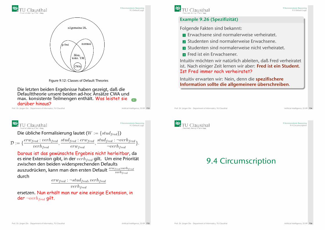
9 Nonmonotonic Reasoning9.3 Default Logic
Figure 9.12: Classes of Default Theories
Die letzten beiden Ergebnisse haben gezeigt, daß dieDefaulttheorie unsere beiden ad-hoc Ansätze CWA undmax. konsistente Teilmengen enthält. Was leistet siedarüber hinaus?
Prof. Dr. Jürgen Dix · Department of Informatics, TU Clausthal Artificial Intelligence, SS 09 733
9 Nonmonotonic Reasoning9.3 Default Logic
Example 9.26 (Spezifizität)
Folgende Fakten sind bekannt:1 Erwachsene sind normalerweise verheiratet.2 Studenten sind normalerweise Erwachsene.3 Studenten sind normalerweise nicht verheiratet.4 Fred ist ein Erwachsener.
Intuitiv möchten wir natürlich ableiten, daß Fred verheiratetist. Nach einiger Zeit lernen wir aber: Fred ist ein Student.Ist Fred immer noch verheiratet?Intuitiv erwarten wir: Nein, denn die spezifischereInformation sollte die allgemeinere überschreiben.
Prof. Dr. Jürgen Dix · Department of Informatics, TU Clausthal Artificial Intelligence, SS 09 734
9 Nonmonotonic Reasoning9.3 Default Logic
Die übliche Formalisierung lautet (W := {studfred})
D := {erwfred : verhfredverhfred
,studfred : erwfred
erwfred,studfred : ¬verhfred
¬verhfred}.
Daraus ist das gewünschte Ergebnis nicht herleitbar, daes eine Extension gibt, in der verhfred gilt. Um eine Prioritätzwischen den beiden widersprechenden Defaultsauszudrücken, kann man den ersten Default erwfred:verhfred
verhfred
durcherwfred : ¬studfred, verhfred
verhfred
ersetzen. Nun erhält man nur eine einzige Extension, inder ¬verhfred gilt.
Prof. Dr. Jürgen Dix · Department of Informatics, TU Clausthal Artificial Intelligence, SS 09 735
9 Nonmonotonic Reasoning9.4 Circumscription
9.4 Circumscription
Prof. Dr. Jürgen Dix · Department of Informatics, TU Clausthal Artificial Intelligence, SS 09 736
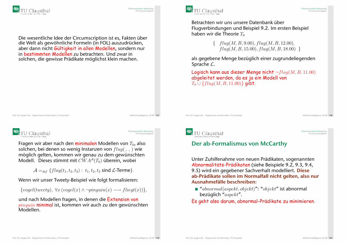
9 Nonmonotonic Reasoning9.4 Circumscription
Die wesentliche Idee der Circumscription ist es, Fakten überdie Welt als gewöhnliche Formeln (in FOL) auszudrücken,aber dann nicht Gültigkeit in allen Modellen, sondern nurin bestimmten Modellen zu betrachten. Und zwar insolchen, die gewisse Prädikate möglichst klein machen.
Prof. Dr. Jürgen Dix · Department of Informatics, TU Clausthal Artificial Intelligence, SS 09 737
9 Nonmonotonic Reasoning9.4 Circumscription
Betrachten wir uns unsere Datenbank überFlugverbindungen und Beispiel 9.2. Im ersten Beispielhaben wir die Theorie T0
{ flug(M,B, 9.00), f lug(M,B, 12.00),f lug(M,B, 15.00), f lug(M,B, 18.00) }
als gegebene Menge bezüglich einer zugrundeliegendenSprache L.
Logisch kann aus dieser Menge nicht ¬flug(M,B, 11.00)abgeleitet werden, da es ja ein Modell vonT0 ∪ {flug(M,B, 11.00)} gibt.
Prof. Dr. Jürgen Dix · Department of Informatics, TU Clausthal Artificial Intelligence, SS 09 738
9 Nonmonotonic Reasoning9.4 Circumscription
Fragen wir aber nach den minimalen Modellen von T0, alsosolchen, bei denen so wenig Instanzen von flug( , , ) wiemöglich gelten, kommen wir genau zu dem gewünschtenModell. Dieses stimmt mit CWAA(T0) überein, wobei
A =def {flug(t1, t2, t3) : t1, t2, t3 sind L-Terme}.
Wenn wir unser Tweety-Beispiel wie folgt formalisieren:
{vogel(tweety), ∀x (vogel(x) ∧ ¬pinguin(x) −→ fliegt(x))},
und nach Modellen fragen, in denen die Extension vonpinguin minimal ist, kommen wir auch zu den gewünschtenModellen.
Prof. Dr. Jürgen Dix · Department of Informatics, TU Clausthal Artificial Intelligence, SS 09 739
9 Nonmonotonic Reasoning9.4 Circumscription
Der ab-Formalismus von McCarthy
Unter Zuhilfenahme von neuen Prädikaten, sogenanntenAbnormalitäts-Prädikaten (siehe Beispiele 9.2, 9.3, 9.4,9.5) wird ein gegebener Sachverhalt modelliert. Dieseab-Prädikate sollen im Normalfall nicht gelten, also nurAusnahmefälle beschreiben:
“abnormal(aspekt, objekt)”: “objekt” ist abnormalbezüglich “aspekt”.
Es geht also darum, abnormal-Prädikate zu minimieren.
Prof. Dr. Jürgen Dix · Department of Informatics, TU Clausthal Artificial Intelligence, SS 09 740
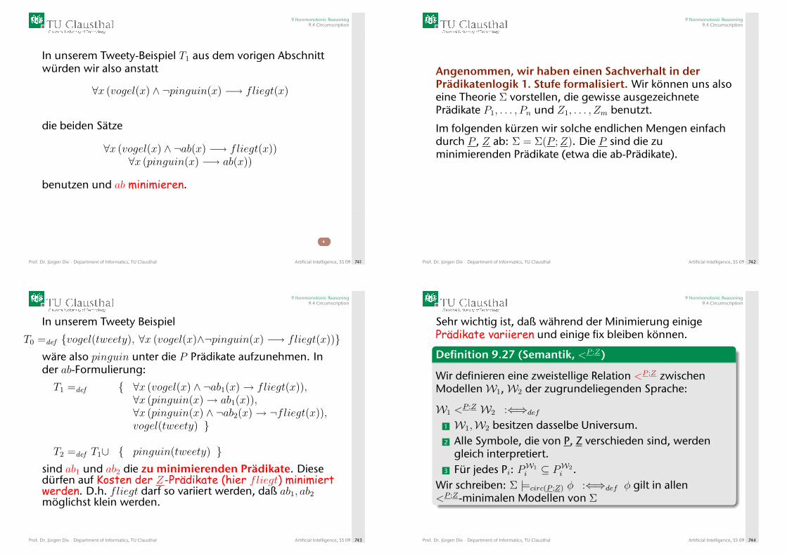
9 Nonmonotonic Reasoning9.4 Circumscription
In unserem Tweety-Beispiel T1 aus dem vorigen Abschnittwürden wir also anstatt
∀x (vogel(x) ∧ ¬pinguin(x) −→ fliegt(x)
die beiden Sätze
∀x (vogel(x) ∧ ¬ab(x) −→ fliegt(x))∀x (pinguin(x) −→ ab(x))
benutzen und ab minimieren.
Prof. Dr. Jürgen Dix · Department of Informatics, TU Clausthal Artificial Intelligence, SS 09 741
9 Nonmonotonic Reasoning9.4 Circumscription
Angenommen, wir haben einen Sachverhalt in derPrädikatenlogik 1. Stufe formalisiert. Wir können uns alsoeine Theorie Σ vorstellen, die gewisse ausgezeichnetePrädikate P1, . . . , Pn und Z1, . . . , Zm benutzt.
Im folgenden kürzen wir solche endlichen Mengen einfachdurch P , Z ab: Σ = Σ(P ;Z). Die P sind die zuminimierenden Prädikate (etwa die ab-Prädikate).
Prof. Dr. Jürgen Dix · Department of Informatics, TU Clausthal Artificial Intelligence, SS 09 742
9 Nonmonotonic Reasoning9.4 Circumscription
In unserem Tweety Beispiel
T0 =def {vogel(tweety), ∀x (vogel(x)∧¬pinguin(x) −→ fliegt(x))}wäre also pinguin unter die P Prädikate aufzunehmen. Inder ab-Formulierung:
T1 =def { ∀x (vogel(x) ∧ ¬ab1(x)→ fliegt(x)),∀x (pinguin(x)→ ab1(x)),∀x (pinguin(x) ∧ ¬ab2(x)→ ¬fliegt(x)),vogel(tweety) }
T2 =def T1∪ { pinguin(tweety) }sind ab1 und ab2 die zu minimierenden Prädikate. Diesedürfen auf Kosten der Z-Prädikate (hier fliegt) minimiertwerden. D.h. fliegt darf so variiert werden, daß ab1, ab2
möglichst klein werden.
Prof. Dr. Jürgen Dix · Department of Informatics, TU Clausthal Artificial Intelligence, SS 09 743
9 Nonmonotonic Reasoning9.4 Circumscription
Sehr wichtig ist, daß während der Minimierung einigePrädikate variieren und einige fix bleiben können.
Definition 9.27 (Semantik, <P ;Z)
Wir definieren eine zweistellige Relation <P ;Z zwischenModellenW1,W2 der zugrundeliegenden Sprache:
W1 <P ;Z W2 :⇐⇒def
1 W1,W2 besitzen dasselbe Universum.2 Alle Symbole, die von P, Z verschieden sind, werden
gleich interpretiert.3 Für jedes Pi: PW1
i ⊆ PW2i .
Wir schreiben: Σ |=circ(P ;Z) φ :⇐⇒def φ gilt in allen<P ;Z-minimalen Modellen von Σ
Prof. Dr. Jürgen Dix · Department of Informatics, TU Clausthal Artificial Intelligence, SS 09 744
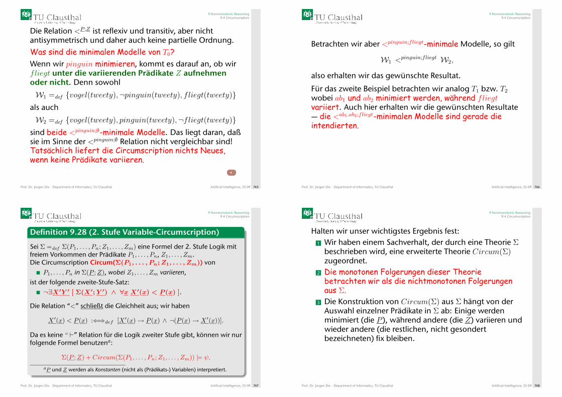
9 Nonmonotonic Reasoning9.4 Circumscription
Die Relation <P ;Z ist reflexiv und transitiv, aber nichtantisymmetrisch und daher auch keine partielle Ordnung.Was sind die minimalen Modelle von T0?Wenn wir pinguin minimieren, kommt es darauf an, ob wirfliegt unter die variierenden Prädikate Z aufnehmenoder nicht. Denn sowohl
W1 =def {vogel(tweety),¬pinguin(tweety), f liegt(tweety)}als auch
W2 =def {vogel(tweety), pinguin(tweety),¬fliegt(tweety)}sind beide <pinguin;∅-minimale Modelle. Das liegt daran, daßsie im Sinne der <pinguin;∅ Relation nicht vergleichbar sind!Tatsächlich liefert die Circumscription nichts Neues,wenn keine Prädikate variieren.
Prof. Dr. Jürgen Dix · Department of Informatics, TU Clausthal Artificial Intelligence, SS 09 745
9 Nonmonotonic Reasoning9.4 Circumscription
Betrachten wir aber <pinguin;fliegt-minimale Modelle, so gilt
W1 <pinguin;fliegt W2,
also erhalten wir das gewünschte Resultat.
Für das zweite Beispiel betrachten wir analog T1 bzw. T2
wobei ab1 und ab2 minimiert werden, während fliegtvariiert. Auch hier erhalten wir die gewünschten Resultate— die <ab1,ab2;fliegt-minimalen Modelle sind gerade dieintendierten.
Prof. Dr. Jürgen Dix · Department of Informatics, TU Clausthal Artificial Intelligence, SS 09 746
9 Nonmonotonic Reasoning9.4 Circumscription
Definition 9.28 (2. Stufe Variable-Circumscription)
Sei Σ =def Σ(P1, . . . , Pn;Z1, . . . , Zm) eine Formel der 2. Stufe Logik mitfreiem Vorkommen der Prädikate P1, . . . , Pn, Z1, . . . , Zm.Die Circumscription Circum(Σ(P1, . . . , Pn; Z1, . . . , Zm)) von
P1, . . . , Pn in Σ(P ;Z), wobei Z1, . . . , Zm variieren,ist der folgende zweite-Stufe-Satz:¬∃X′Y ′ [ Σ(X′; Y ′) ∧ ∀x X′(x) < P (x) ].
Die Relation “<” schließt die Gleichheit aus; wir haben
X ′(x) < P (x) :⇐⇒def [X ′(x)→ P (x) ∧ ¬(P (x)→ X ′(x))].
Da es keine “ `” Relation für die Logik zweiter Stufe gibt, können wir nurfolgende Formel benutzena:
Σ(P ;Z) + Circum(Σ(P1, . . . , Pn;Z1, . . . , Zm)) |= ψ.aP und Z werden als Konstanten (nicht als (Prädikats-) Variablen) interpretiert.
Prof. Dr. Jürgen Dix · Department of Informatics, TU Clausthal Artificial Intelligence, SS 09 747
9 Nonmonotonic Reasoning9.4 Circumscription
Halten wir unser wichtigstes Ergebnis fest:1 Wir haben einem Sachverhalt, der durch eine Theorie Σ
beschrieben wird, eine erweiterte Theorie Circum(Σ)zugeordnet.
2 Die monotonen Folgerungen dieser Theoriebetrachten wir als die nichtmonotonen Folgerungenaus Σ.
3 Die Konstruktion von Circum(Σ) aus Σ hängt von derAuswahl einzelner Prädikate in Σ ab: Einige werdenminimiert (die P ), während andere (die Z) variieren undwieder andere (die restlichen, nicht gesondertbezeichneten) fix bleiben.
Prof. Dr. Jürgen Dix · Department of Informatics, TU Clausthal Artificial Intelligence, SS 09 748
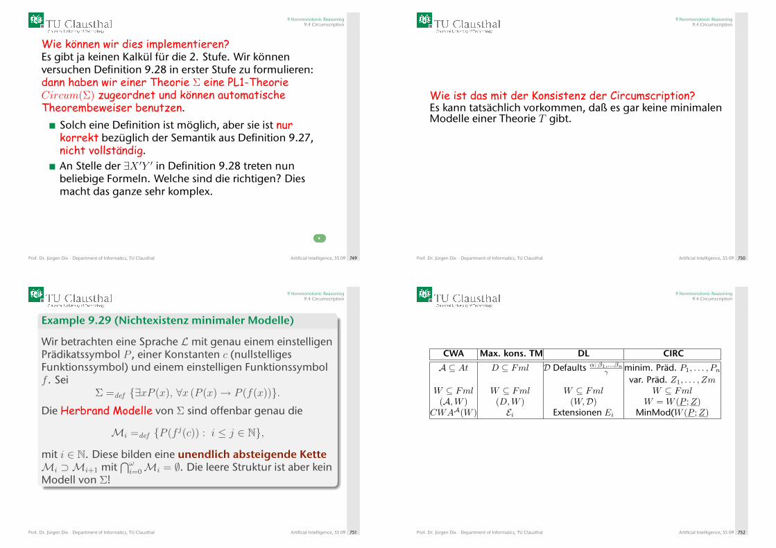
9 Nonmonotonic Reasoning9.4 Circumscription
Wie können wir dies implementieren?Es gibt ja keinen Kalkül für die 2. Stufe. Wir könnenversuchen Definition 9.28 in erster Stufe zu formulieren:dann haben wir einer Theorie Σ eine PL1-TheorieCircum(Σ) zugeordnet und können automatischeTheorembeweiser benutzen.
Solch eine Definition ist möglich, aber sie ist nurkorrekt bezüglich der Semantik aus Definition 9.27,nicht vollständig.An Stelle der ∃X ′Y ′ in Definition 9.28 treten nunbeliebige Formeln. Welche sind die richtigen? Diesmacht das ganze sehr komplex.
Prof. Dr. Jürgen Dix · Department of Informatics, TU Clausthal Artificial Intelligence, SS 09 749
9 Nonmonotonic Reasoning9.4 Circumscription
Wie ist das mit der Konsistenz der Circumscription?Es kann tatsächlich vorkommen, daß es gar keine minimalenModelle einer Theorie T gibt.
Prof. Dr. Jürgen Dix · Department of Informatics, TU Clausthal Artificial Intelligence, SS 09 750
9 Nonmonotonic Reasoning9.4 Circumscription
Example 9.29 (Nichtexistenz minimaler Modelle)
Wir betrachten eine Sprache Lmit genau einem einstelligenPrädikatssymbol P , einer Konstanten c (nullstelligesFunktionssymbol) und einem einstelligen Funktionssymbolf . Sei
Σ =def {∃xP (x), ∀x (P (x)→ P (f(x))}.Die Herbrand Modelle von Σ sind offenbar genau die
Mi =def {P (f j(c)) : i ≤ j ∈ N},
mit i ∈ N. Diese bilden eine unendlich absteigende KetteMi ⊃Mi+1 mit
⋂ωi=0Mi = ∅. Die leere Struktur ist aber kein
Modell von Σ!
Prof. Dr. Jürgen Dix · Department of Informatics, TU Clausthal Artificial Intelligence, SS 09 751
9 Nonmonotonic Reasoning9.4 Circumscription
CWA Max. kons. TM DL CIRC
A ⊆ At D ⊆ Fml D Defaults α: β1,...βn
γ minim. Präd. P1, . . . , Pnvar. Präd. Z1, . . . , Zm
W ⊆ Fml W ⊆ Fml W ⊆ Fml W ⊆ Fml(A,W ) (D,W ) (W,D) W = W (P ;Z)
CWAA(W ) Ei Extensionen Ei MinMod(W (P ;Z)
Prof. Dr. Jürgen Dix · Department of Informatics, TU Clausthal Artificial Intelligence, SS 09 752
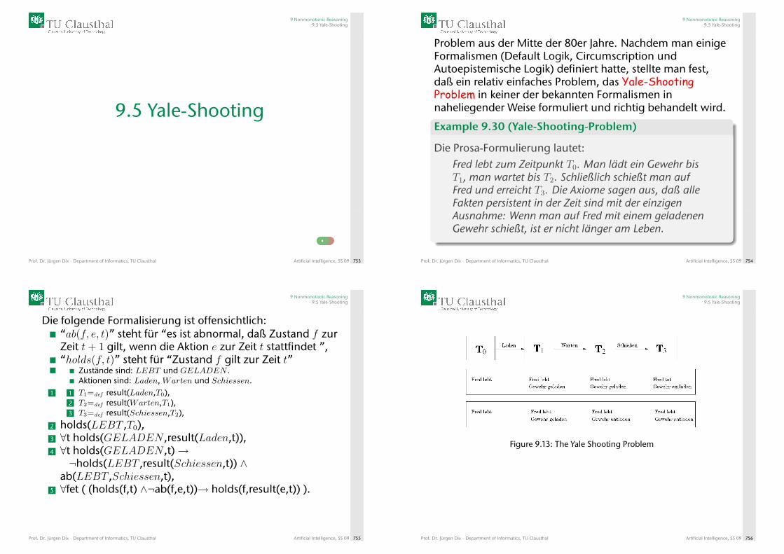
9 Nonmonotonic Reasoning9.5 Yale-Shooting
9.5 Yale-Shooting
Prof. Dr. Jürgen Dix · Department of Informatics, TU Clausthal Artificial Intelligence, SS 09 753
9 Nonmonotonic Reasoning9.5 Yale-Shooting
Problem aus der Mitte der 80er Jahre. Nachdem man einigeFormalismen (Default Logik, Circumscription undAutoepistemische Logik) definiert hatte, stellte man fest,daß ein relativ einfaches Problem, das Yale-ShootingProblem in keiner der bekannten Formalismen innaheliegender Weise formuliert und richtig behandelt wird.
Example 9.30 (Yale-Shooting-Problem)
Die Prosa-Formulierung lautet:Fred lebt zum Zeitpunkt T0. Man lädt ein Gewehr bisT1, man wartet bis T2. Schließlich schießt man aufFred und erreicht T3. Die Axiome sagen aus, daß alleFakten persistent in der Zeit sind mit der einzigenAusnahme: Wenn man auf Fred mit einem geladenenGewehr schießt, ist er nicht länger am Leben.
Prof. Dr. Jürgen Dix · Department of Informatics, TU Clausthal Artificial Intelligence, SS 09 754
9 Nonmonotonic Reasoning9.5 Yale-Shooting
Die folgende Formalisierung ist offensichtlich:“ab(f, e, t)” steht für “es ist abnormal, daß Zustand f zurZeit t+ 1 gilt, wenn die Aktion e zur Zeit t stattfindet ”,“holds(f, t)” steht für “Zustand f gilt zur Zeit t”
Zustände sind: LEBT und GELADEN .Aktionen sind: Laden, Warten und Schiessen.
1 1 T1=def result(Laden,T0),2 T2=def result(Warten,T1),3 T3=def result(Schiessen,T2),
2 holds(LEBT ,T0),3 ∀t holds(GELADEN ,result(Laden,t)),4 ∀t holds(GELADEN ,t)→¬holds(LEBT ,result(Schiessen,t)) ∧
ab(LEBT ,Schiessen,t),5 ∀fet ( (holds(f,t) ∧¬ab(f,e,t))→ holds(f,result(e,t)) ).
Prof. Dr. Jürgen Dix · Department of Informatics, TU Clausthal Artificial Intelligence, SS 09 755
9 Nonmonotonic Reasoning9.5 Yale-Shooting
Figure 9.13: The Yale Shooting Problem
Prof. Dr. Jürgen Dix · Department of Informatics, TU Clausthal Artificial Intelligence, SS 09 756

9 Nonmonotonic Reasoning9.5 Yale-Shooting
Wenn wir die Circumscription dieser Theorie betrachtenund ab(f, e, t) minimieren, so existiert immer ein minimalesModell in dem gilt:
1 ab(GELADEN,Warten, T1) (das Gewehr entlud sich),2 ¬holds(GELADEN, T2) und3 holds(LEBT, T3).
Das eigentlich intendierte Modell, nämlich1 ab(LEBT, Schiessen, T2),2 holds(GELADEN, T2) und3 ¬holds(LEBT, T3).
ist mit dem ersten nicht vergleichbar, beide sind minimal!
Prof. Dr. Jürgen Dix · Department of Informatics, TU Clausthal Artificial Intelligence, SS 09 757
9 Nonmonotonic Reasoning9.5 Yale-Shooting
Dasselbe Problem tritt auf, wenn man die Default Logikbenutzt. Man kann dann die obige Formulierungbeibehalten (natürlich muß man alles in Aussagenlogikformulieren, da wir DL ja nur für LAL eingeführt haben) undmuß nur noch die Defaults
für alle f, e, t: ∅:¬ab(f,e,t)¬ab(f,e,t)
hinzunehmen.Auch hier erhält man allerdings die Existenz von zweiExtensionen (den beiden gerade beschriebenen Modellen)anstatt einer einzigen.
Prof. Dr. Jürgen Dix · Department of Informatics, TU Clausthal Artificial Intelligence, SS 09 758
9 Nonmonotonic Reasoning9.5 Yale-Shooting
Das Problem ist daher,1 im Voraus die gewünschten Extensionen zu
charakterisieren, oder äquivalent dazu, das richtigeminimale1 Modell auszuwählen,
2 eine uniforme Methode anzugeben, wie man Defaultsformulieren muß, damit die ungewollten Extensionennicht auftreten.
1wobei ab zu minimieren ist
Prof. Dr. Jürgen Dix · Department of Informatics, TU Clausthal Artificial Intelligence, SS 09 759