1

Art as an Investment and the Underperformance of Masterpieces

Jiangping Mei

Michael Moses∗

February 2002

Abstract

This paper constructs a new data set of repeated sales of artworks and estimates an annual

index of art prices for the period 1875-2000. Contrary to earlier studies, we find art outperforms

fixed income securities as an investment, though it significantly under-performs stocks in the

US. Art is also found to have lower volatility and lower correlation with other assets, making it

more attractive for portfolio diversification than discovered in earlier research. There is strong

evidence of underperformance of masterpieces, meaning expensive paintings tend to under-

perform the art market index. The evidence is mixed on whether the "law of one price" holds in

the New York auction market.

(JEL G11, G12, Z10)

∗ Department of Finance and Department of Operations Management, Stern School of Business, New York University, 44 West 4th Street, New York, NY 10012-1126. We like to thank Orley Ashenfelter (the co-editor) and two anonymous referees for their numerous helpful comments. We have benefited from discussions with Will Goetzmann, Robert Solow and Larry White on art as an investment. We are grateful to Jennifer Bowe, Jin Hung and Loan Hong for able research assistance. We would also like to thank Mathew Gee of the Stern Computer Department for his tireless efforts in rationalizing our database. We also wish to thank John Ammer, John Campbell, Victor Ginsburgh, Robert Hodrick, Burton Malkiel, Tom Pugel, and seminar participants at Temple University and New York University for helpful comments. All errors remain ours. Additional information about the art price indices is available from www.meimosesfineartindex.org.

2

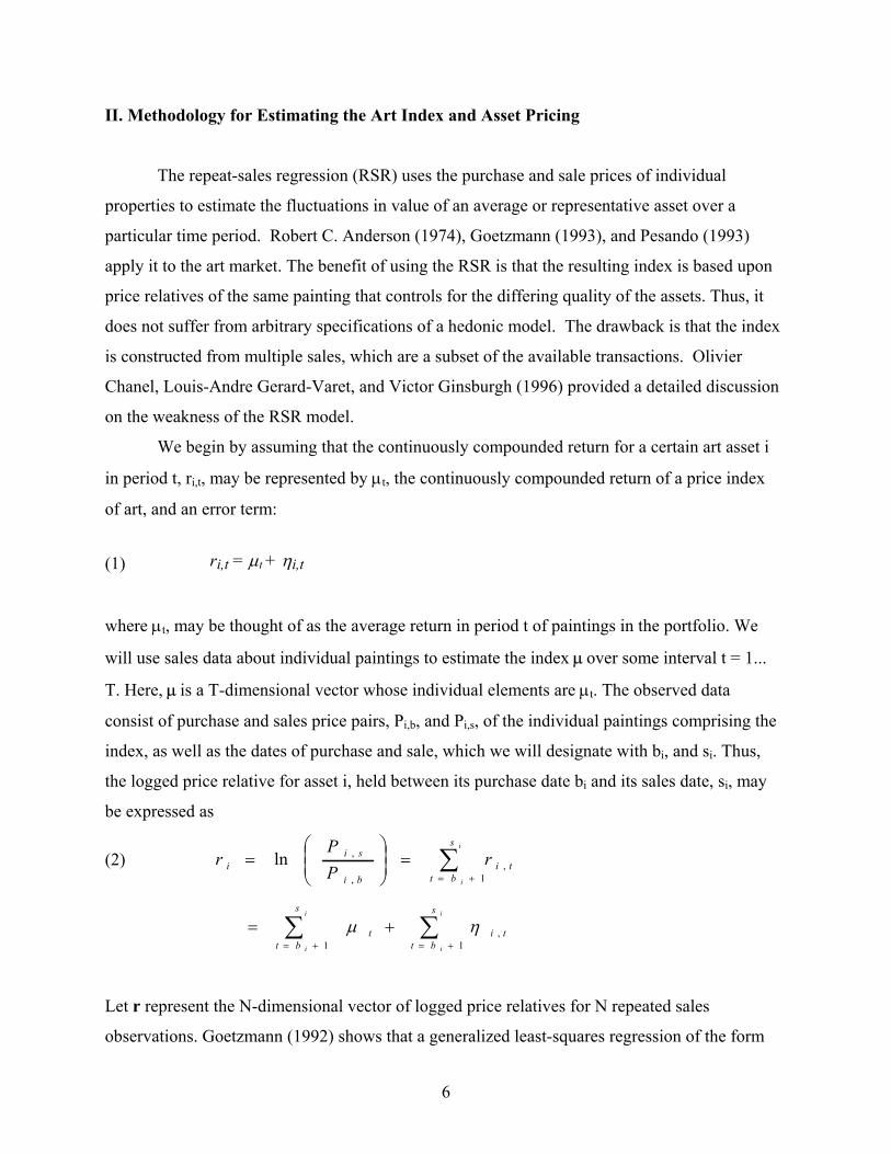
Two major obstacles in analyzing the art market are heterogeneity of artworks and

infrequency of trading. The present paper overcomes these problems by constructing a new

repeated-sales data set based on auction art price records at the New York Public Library as well

as the Watson Library at the Metropolitan Museum of Art. As a result, we have a significant

increase in the number of repeated sales compared to earlier studies by William J. Baumol

(1986) and William N. Goetzmann (1993).1 For the artworks included in the present study, we

have 4,896 price pairs covering the period 1875-2000. With a larger data set, we are able to

construct an annual art index as well as annual sub-indices for American, Old Master,

Impressionist and Modern paintings for various time periods. The annual indices are then used to

address the question of whether the risk-return characteristics of paintings compare favorably to

those of traditional financial assets, such as stocks and bonds.

The larger data set also permits us to test two propositions frequently advanced by art

dealers and economists. The first one states that art investors should buy only the top works of

established artists (masterpieces) or buy the most expensive artwork they can afford. The

empirical evidence on the return performance of masterpieces is mixed. James E. Pesando (1993)

presented strong evidence of underperformance while Goetzmann (1996) found no such

evidence. Our study will extend their analysis with a new testing procedure based on repeated

sales regression (RSR).

The second proposition states that prices realized for identical paintings at different

locations at the same time should be the same. Pesando (1993) compared prices of alternate

copies of the same prints sold at Sotheby’s and Christie’s in New York and found substantial

evidence of violation of the “law of one price” during the 1977-1992 period. While no art piece

in our data has ever been sold simultaneously in both auction houses, we will conduct a test of

the “law of one price” by examining return differentials for artworks sold at different auction

houses over much longer time periods. If there is systematic pricing bias from one auction house

to the other, then we should expect to see systematic difference in returns for artworks sold at

1 Goetzmann (1993) uses price data recorded by Gerald Reitlinger (1961) and Enrique Mayer (1971-1987) to construct a decade art index based on paintings which sold two or more times, during the period 1715-1986. His data set contains 3,329 price pairs. Baumol (1986) uses a subset of the data recorded by Reitlinger (1961) to study the returns on paintings during the period 1652-1961. His data set contains 640 price pairs. Buelens and Ginsburgh (1993) re-exams Baumol’s work with different sample periods. Pesando (1993) uses data for repeat sales of modern prints which has 27,961 repeat sales. But his data only covers a short time span from 1977 to 1992.

3

different houses. We will examine the return differentials with a RSR procedure that is different

from Pesando (1993).

The remainder of the paper is organized as follows. Section I describes the art auction

data set and provides a discussion of sampling biases. Section II reviews the repeated sales

regression procedure used to estimate the index for painting prices and provides an asset-pricing

framework for estimating the systematic risk of paintings. Section III provides risk and return

characteristics of the estimated art price index. Section IV presents evidence on the

underperformance of masterpieces. Section V tests the hypothesis of the "law of one price" while

Section VI concludes the paper.

I. Painting Data and Biases

Since individual works of art have yet to be securitized nor are there publicly traded art

funds, studying the value of works of art from financial sources is not possible. Gallery or

direct-from-artists prices tend not to be reliable or easily obtainable. Repeat sale auction prices

however are reliable and publicly available (in catalogues) and can be used as the basis for a

data base for determining the change in value of art objects over various holding periods and

collecting categories.

We created such a database for the American market, principally New York. For the

second half of the 20th Century we searched the catalogues for all American, 19th Century and

Old Master, Impressionist and Modern paintings sold at the main sales rooms of Sotheby's and

Christie’s (and their predecessor firms) from 1950 to 2000.2 If a painting had listed in its

provenance a prior public sale, at any auction house anywhere, we went back to that auction

catalogue and recorded the sale price. The New York Public Library as well as the Watson

Library at the Metropolitan Museum of Art were our major sources for this auction price

history. Some paintings had multiple resales over many years resulting in up to six resales for

some works of art. Each resale pair was considered a unique point in our database that now

totals over five thousand entries. Some of the original purchase dates went back to the 17th

century. If the art piece was sold overseas, we converted the sale price into US dollars using the

2 Our data does not include "bought-in" paintings that did not sell due to the fact that the bid was below reservation price. Our data for the year 2000 only includes sales before July.

4

long-term exchange rate data provided by Global Financial Data. Our data has continuous

observations since 1871 and has numerous observations that allow us to develop an annual art

index since 1875.

As well as analyzing our data as a totality we have also separated it into three popular

collecting categories. The first is American Paintings (American) principally created between

1700 and 1950. The second is Impressionist and Modern Paintings (Impressionists) principally

created between the third quarters of the 19th and 20th century. The third is Old Master and 19th

century paintings (Old Masters) principally created after the 12th century and before the third

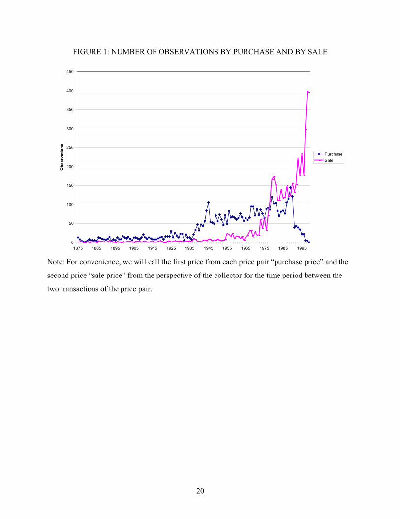
quarter of the 19th century. The number of observations in our resale data by year of purchase

and sale from 1875-2000 are depicted in Figure 1. For convenience, we will call the first price

from each price pair “purchase price” and the second price “sale price” from the perspective of

the collector for the time period between the two transactions corresponding to the price pair.

The database for this time period contains 4,896 price pairs, consisting of 899 pairs from

American, 1,709 from Impressionist, and 2,288 from Old Masters. We can see that our data is

rather spotty for the beginning of our sample but increases rapidly after 1935.3 We can also see

that most artworks bought are held for long time periods (on average 28 years) so that not many

purchases in the early years are sold right away.

The selection bias in the data set is an important issue that bears on the interpretation of

our empirical study. The selection procedures based on multiple sales from major US auction

houses tend to truncate both sides of the return distribution. Our sample may suffer from a

“backward filled” data bias since our transactions data before 1950 are collected only from

those paintings that were sold in Christie’s and Sotheby’s after 1950.4 Given the reputation of

the two auction houses, our data may have a bias toward those paintings that have a high value

3 Note that the scarcity of “sales” data before 1935 was compensated to some extent by more “purchase” data in the repeated sales regression, which use both sets of data in the construction of the art market index. However, the scarcity of data before 1935 would impact the volatility of the index since the art index portfolio then was poorly diversified because of few artworks in the portfolio. 4 This bias is similar to the “back-filled” data bias for emerging market stocks where historical data on their returns is “back-filled” conditional upon the survival of emerging markets. Thus, data for those emerging markets that submerged as result of revolution or economic turmoil were not included, which tend to create a downward bias. See Campbell Harvey (1995) for a detailed discussion. We like to note, however, unlike Russian bonds and Cuban stocks, paintings from established artists sold in auctions seldom disappear from the market completely. Thus, one can still observe a large number of art pieces sold at estate auctions at a fraction of their purchase price.

5

after 1950. However, this “backward filled” bias is mitigated by two facts: first, our data set

does have a large number of paintings with poor returns. This is partly due to the fact that

auction houses are obliged to sell all estate holdings whether they have high values or not.

Auction houses such as Sotheby’s and Christie’s also have incentives to sell inexpensive

artworks from established artists to attract first time collectors. Thus, we do observe prices of

artworks that had fallen substantially. Second, our data before 1950 also come from well known

auction houses around the world, so our data principally include works of artists established at

the time of purchase. This will tend to moderate the upward bias of our return estimates due to

survival. Moreover, expensive paintings today that were bought a long time ago at low prices

directly from dealers or artists are not included in our sample due to the lack of transaction

records. This will partially offset the upward bias as well. Moreover, masterpieces collected by

museums through donation rather than auction sales are also excluded from the sample, further

offsetting the upward bias.

In addition to these selection biases, Orley Ashenfelter, Kathryn Graddy, and Margaret

Stevens (2001) pointed out that not all items that are put up for sale at auctions are sold because

some final bids may not reach the reservation prices. Goetzmann (1993) also argues that the

decision by an owner to sell a work of art (and consequently the occurrence of a repeat sale in

the sample) could be conditional upon whether or not the value has increased. These would also

tend to bias the estimated return upward.5 Because of these biases, the mean annual return to art

investment provided by repeated-sale data should be regarded as approximate, or as an upper

bound on the average return obtained by investors over the period. The return could be further

reduced by transaction costs. We like to note, however, that return estimates for financial assets,

to some extent, also could suffer from the same biases, such as lack of market liquidity,

transaction costs and survival.

5 Goetzmann (1993, 1996) also argues that auction transactions may not adequately reflect an important element of risk for the art investor: stylistic risk. In other words, the future sales price will depend upon the number of people who wish to buy the work of art when it is put up for sale. Since the repeat-sales data principally reflect auction transactions, they necessarily focus upon artworks that have a broad demand to attract a large number of competitive bidders. Thus, the repeat-sales records will fail to capture the price fluctuations of paintings that are not broadly in demand. The stylistic risk is similar in many respects to the liquidity risk in financial markets, where prices of assets are affected not only by fundamental values but also by market liquidity.

6

II. Methodology for Estimating the Art Index and Asset Pricing

The repeat-sales regression (RSR) uses the purchase and sale prices of individual

properties to estimate the fluctuations in value of an average or representative asset over a

particular time period. Robert C. Anderson (1974), Goetzmann (1993), and Pesando (1993)

apply it to the art market. The benefit of using the RSR is that the resulting index is based upon

price relatives of the same painting that controls for the differing quality of the assets. Thus, it

does not suffer from arbitrary specifications of a hedonic model. The drawback is that the index

is constructed from multiple sales, which are a subset of the available transactions. Olivier

Chanel, Louis-Andre Gerard-Varet, and Victor Ginsburgh (1996) provided a detailed discussion

on the weakness of the RSR model.

We begin by assuming that the continuously compounded return for a certain art asset i

in period t, ri,t, may be represented by µt, the continuously compounded return of a price index

of art, and an error term:

(1) ri,t = µt + ηi,t

where µt, may be thought of as the average return in period t of paintings in the portfolio. We

will use sales data about individual paintings to estimate the index µ over some interval t = 1...

T. Here, µ is a T-dimensional vector whose individual elements are µt. The observed data

consist of purchase and sales price pairs, Pi,b, and Pi,s, of the individual paintings comprising the

index, as well as the dates of purchase and sale, which we will designate with bi, and si. Thus,

the logged price relative for asset i, held between its purchase date bi and its sales date, si, may

be expressed as

(2) ∑+=

=

=

i

i

s

btti

bi

sii r

PP

r1

,,

,ln

∑ ∑+= +=

+=i

i

i

i

s

bt

s

bttit

1 1,ηµ

Let r represent the N-dimensional vector of logged price relatives for N repeated sales

observations. Goetzmann (1992) shows that a generalized least-squares regression of the form

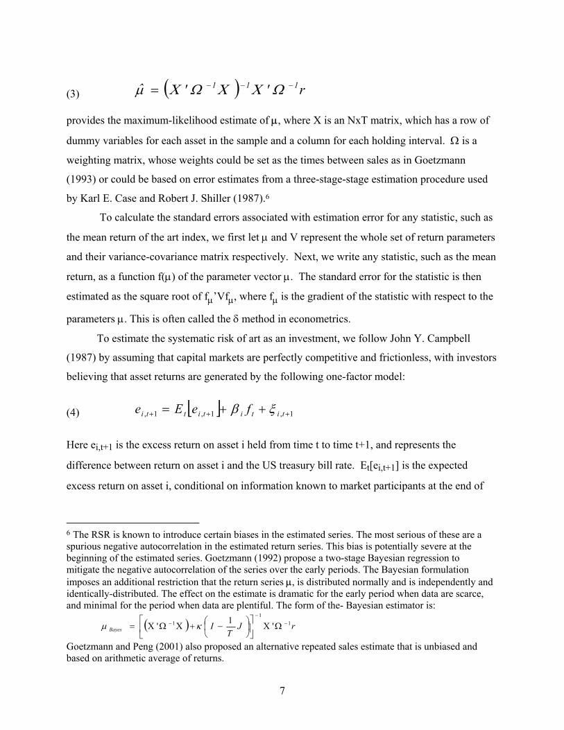
7

(3) ( ) r''ˆ 111 −−−= ΩΧΧΩΧµ provides the maximum-likelihood estimate of µ, where X is an NxT matrix, which has a row of

dummy variables for each asset in the sample and a column for each holding interval. Ω is a

weighting matrix, whose weights could be set as the times between sales as in Goetzmann

(1993) or could be based on error estimates from a three-stage-stage estimation procedure used

by Karl E. Case and Robert J. Shiller (1987).6

To calculate the standard errors associated with estimation error for any statistic, such as

the mean return of the art index, we first let µ and V represent the whole set of return parameters

and their variance-covariance matrix respectively. Next, we write any statistic, such as the mean

return, as a function f(µ) of the parameter vector µ. The standard error for the statistic is then

estimated as the square root of fµ’Vfµ, where fµ is the gradient of the statistic with respect to the

parameters µ. This is often called the δ method in econometrics.

To estimate the systematic risk of art as an investment, we follow John Y. Campbell

(1987) by assuming that capital markets are perfectly competitive and frictionless, with investors

believing that asset returns are generated by the following one-factor model:

(4) [ ] 1,1,1, +++ ++= titititti feEe ξβ

Here ei,t+1 is the excess return on asset i held from time t to time t+1, and represents the

difference between return on asset i and the US treasury bill rate. Et[ei,t+1] is the expected

excess return on asset i, conditional on information known to market participants at the end of

6 The RSR is known to introduce certain biases in the estimated series. The most serious of these are a spurious negative autocorrelation in the estimated return series. This bias is potentially severe at the beginning of the estimated series. Goetzmann (1992) propose a two-stage Bayesian regression to mitigate the negative autocorrelation of the series over the early periods. The Bayesian formulation imposes an additional restriction that the return series µ, is distributed normally and is independently and identically-distributed. The effect on the estimate is dramatic for the early period when data are scarce, and minimal for the period when data are plentiful. The form of the- Bayesian estimator is:

( ) rJT

IBayes1

11 '1' −

−− ΩΧ

−+ΧΩΧ= κµ

Goetzmann and Peng (2001) also proposed an alternative repeated sales estimate that is unbiased and based on arithmetic average of returns.

8

time period t.7 We use the S&P 500 to proxy for the systematic factor and assume Et[ξi,t+1] = 0.

The conditional expected excess return is allowed to vary through time in the current model but

the beta coefficients are assumed to be constant. In computing ei,t, we use return indices from

five different asset class: the Art index, the Dow Jones Industrial Total Return Index, the US

Government Bonds Total Return Index, the US Corporate Bond Total Return Index, and the

United States Treasury Bills Total Return Index. With the exception of the art index, the sources

of these data are from Federal Reserve Board and Global Financial Data (5th edition), which has

derived its data from historical data on prices and yields collected by Standard and Poor’s, the

Cowles Commission, and G. William Schwert (1988). The model is estimated using Lars P.

Hansen's (1982) Generalized Method of Moments (GMM).8

III. Risk and Return Characteristics of the Art Price Index

Figure 2 provides a graphic plot of the art index over the 1875-2000 period with the base

year index set to be 1. The index is estimated with 4,896 pairs of repeated sale prices. Our

reported art index is based on the three-stage-least-square procedure proposed by Case and

Shiller (1987).9 The Adjusted R-squares for the estimation is 0.64, suggesting the art index

explains 64% of the variance of sample return variation. The F-statistic equals 104.32 with a

significance level equal to 0.000, indicating the index is a highly significant common return

component of our art portfolios. Due to a smaller number of observations, the three sub-indices,

American, Impressionist, and Old Masters, were estimated only for the 1941-2000, 1941-2000,

7 We assume [ ] ,

11, ∑

=+ Χ=

L

nntintit eE α where the forecasting variables Xnt include a constant term,

the yield on US treasury bills, the dividend yield on Standard and Poor's 500 index, the dividend payout ratio on the Standard and Poor's 500 index, the spread between the yields on Moody's Baa Corporate Bond and US government bonds, and the spread between the yields on US government bonds and US treasury bills. For more details on the estimation of this model, see Campbell (1987). 8 We have also run OLS regressions of various asset returns directly against the S&P 500 index, assuming the first term to be constant in equation (4). The results are quite similar for all assets except that the estimation errors for betas tend to be larger. These results are available upon request. 9 We use the Case and Shiller (1987) procedure because it allows us to adjust for a downward bias in annual returns estimation due the log price transformation (see Goetzmann (1992)). We have also estimated the art index using GLS and the two-stage Baysian estimation proposed by Goetzmann (1992). The correlation between the Case and Shiller (1987) procedure and the other two procedures are 0.970

9

and 1900-2000 periods respectively. The figure shows a sharp rise in prices in the 1980s with

the art index peaking at 8640 in 1990 followed by a 36% drop in 1991. We can also see that,

even after ten years of market adjustment, the Impressionist Paintings still have not recovered

from its high level of 1990. Thus, total performance has been much affected by the bear market

for art during most of the 1990s. While the boom and bust was well documented in the art

market, the price indices allow us to estimate the precise time and magnitude of the price change.

Our indices have also identified major price drops during the 1974-75 oil crisis and the 1929-

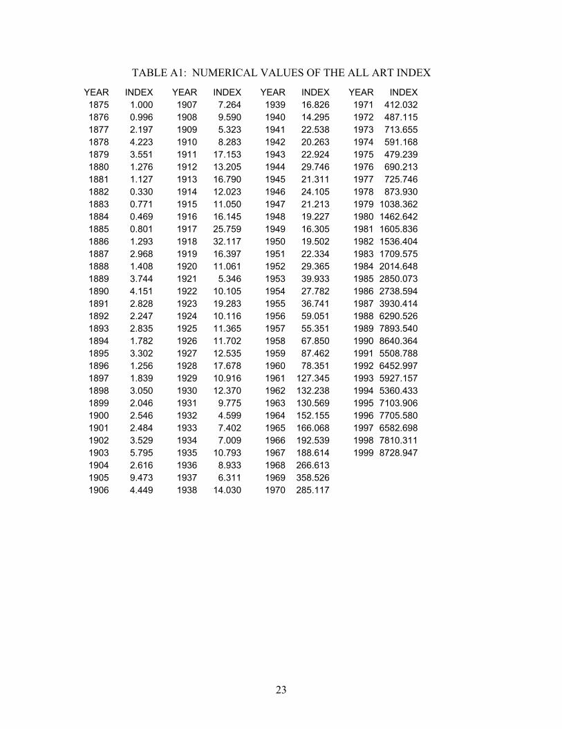
1934 depression. See Appendix for the actual values of the All ART Index.

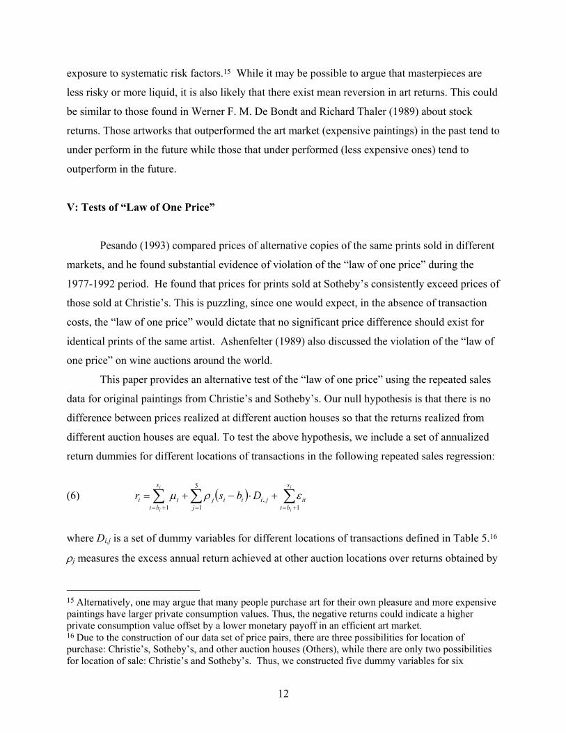
Table 1 provides summary statistics on the behavior of real returns for each of our six asset

classes. The real returns are computed as the nominal return minus annual inflation using the US

CPI index. For each variable, we report the mean, standard deviation, and its correlation with

other assets. We also report the standard deviation of the art return estimates due to estimation

error using the δ method. We can see that our estimates are fairly accurate. The standard error

for the mean return estimate was only 0.2% for the 1950-1999 period and 0.3% for the 1875-

1999 period.10 Table 1 reveals that art had a real annual compounded return of 8.2% comparable

to that of stocks during the 1950-1999 period. Moreover, art out-performed bonds and treasury

bills. Corporate and government bonds derived a 2.2% and 1.9% annual return respectively

while the S&P 500 and the Dow Industrial gained 8.9% and 9.1% respectively. Our results are

quite similar for the 1900-1999 period, though the performance gap between art and stocks

widened. The art index also out-performed fixed income securities during the 1875-1999

period.11 Moreover, we found that the volatility of art market price index dropped to 21.3%

during the 1950-1999 period from 42.8% during the 1875-1999 period, making the art index just

a bit more risky than the two stock indices.12

To compare our results with those obtained in earlier studies, we also estimated real

returns of various assets for the same sample period as in Goetzmann (1993) and Pesando

(1993). The results were reported in the bottom panel of Table 1. While Goetzmann’s art index

and 0.917, suggesting that the results are quite robust. We have also discovered that the two-stage Baysian estimates tend to have smaller estimation errors though they may be biased. 10 We did not include the year 2000, since our data only has sales from the first half of the year. 11 This result is similar to Goetzmann (1993) during the 1850-1986 period. 12 There was a large drop in the volatility of the art index for the most recent sample period. This should be expected, since the number of artworks in our art index portfolio increased rapidly after 1935.

10

significantly out-performed both stocks and bonds during 1900-1986 sample periods, our art

index only outperformed bonds.13 We conjecture that the differences in art performance could be

partly due to a difference in sample selection, since the artists chosen by Reitlinger (1961, 1963

and 1973) could be affected by his taste and other selection biases. This could bias the

performance result upward. In comparison to Goetzmann’s findings, our art index also has less

volatility (and lower correlation with other asset class). This could be the result of our larger

sample, which makes our art index portfolio better diversified and less volatile. Our art index

performed better than that of Pesando (1993) who used modern prints sold in US and Europe. He

found modern prints under-performed both stocks and bonds during the 1977-1992 sample

period. Using semi-annual returns, he also found the print returns could be less volatile than

stock and bonds.14 Because of the lower volatility and correlation with other assets reported in

Table 1, our study suggests that a diversified portfolio of artworks may play a somewhat more

important role in portfolio diversification.

In Table 2, we report the estimates of the one-factor asset pricing model (4). Using the

S&P 500 index as the systematic factor, we observe that the art beta was 0.718 during the sample

period and it was significant with a t-statistic of 3.119. The smaller beta on art compared to the

S&P 500 indicates that art has less systematic risk than the S&P 500 thus it should be expected

to earn a lower return than the S&P 500 over the long run. It also suggests that the art index

tends to move in the same direction as the S&P 500, consistent with a wealth effect from the

stock market discussed in Goetzmann (1993). In addition, the higher systematic risk on art

compared to bonds implies that art should earn a higher return than bonds over the long run.

IV. Do Masterpieces Under-perform?

A common advice given to their clients by art dealers is to buy the best (i.e. most

expensive) artworks they can afford. This presumes that masterpieces of well known artists will

13 It is worth noting that, while both Goetzmann’s (1993) data and our data include artworks sold internationally, Goetzmann’s data are concentrated in UK sales before 1960 and ours are skewed towards auction sales in the US. While our result on art return characteristics is similar to Goetzmann (1996), he did not use a RSR estimation approach in his 1996 paper. 14 Pesando’s volatility numbers are not directly comparable to ours since his computation was based on semiannual data. Our average return results are also similar to those of Buelens and Ginsburgh (1993) from the 1870-1913 period. Their study was also based on the Reitlinger (1961) data.

11

outperform the market. In other words, masterpieces might have a higher expected return than

middle-level and lower-level works of art. Contrary to this popular belief, Pesando (1993)

discovered that masterpieces actually tend to under perform the market. His discovery was based

on repeated sales of modern prints from 1977-1992. Since Pesando’s data only cover prints that

tend to have much lower value when compared to American, Old Masters and Impressionists

paintings, one may wonder if this underperformance exists for truly expensive artworks.

Moreover, Goetzmann (1996) found no evidence of underperformance of masterpieces. Using

repeated sales data covering American, Old Master, Impressionist and Modern paintings, this

paper will further examine the performance of masterpieces. We will follow Pesando by using

the market price to identify the masterpieces (i.e, expensive paintings are masterpieces). In the

first examination, we use prices for all artworks sold between 1875 and 2000. We apply the same

repeated sales regression approach by adding an additional term to equation (2),

(5) ( ) ∑∑+=+=

+Ρ⋅−+=i

i

i

i

s

btitbiii

s

btti bsr

1,

1

ln εγµ

where γ is the elasticity of art returns with respect to log price of the property and (si-bi) is the

holding period. Here γ gives the expected percentage changes in annual returns as a result of a

1% change in art purchase prices. For the three subcategories, we also repeat the same

estimation procedure. In the second exercise, we use prices deflated by the US CPI index, since

the nominal value of art may change due to inflation. The results are reported in Table 3 while

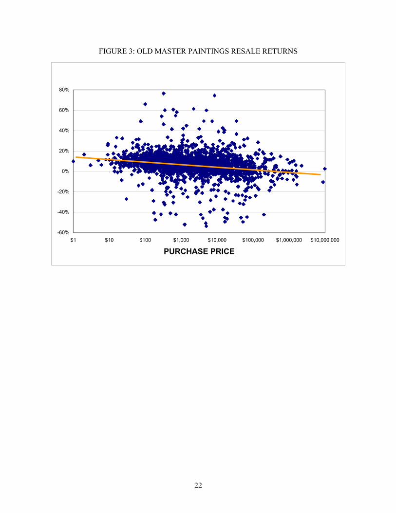
Figure 3 provide a simple plot of art returns and purchase prices for Old Masters paintings. Our

results are uniform across all categories: masterpieces significantly under-performed their

respective art market indices. Our γ estimate on the American artworks indicates that a 10%

increase in purchase price is expected to lower future annual returns by 0.1%. Moreover, our

results are robust to whether nominal prices or real prices are used in the regressions. Thus, our

study seems to suggest that art investors should buy less expensive artworks at auctions.

The underperformance of masterpieces is similar to the “small firm effect” documented

by K.C. Chan and Nai-Fu Chen (1988) and many others in their study of the capital asset pricing

model. These authors discover that small firms with lower market capitalization tend to achieve

excess returns not justified by their risk based on single factor market models. Recent studies by

Eugene Fama and Kenneth French (1995), however, suggest that firm size could be a proxy for

12

exposure to systematic risk factors.15 While it may be possible to argue that masterpieces are

less risky or more liquid, it is also likely that there exist mean reversion in art returns. This could

be similar to those found in Werner F. M. De Bondt and Richard Thaler (1989) about stock

returns. Those artworks that outperformed the art market (expensive paintings) in the past tend to

under perform in the future while those that under performed (less expensive ones) tend to

outperform in the future.

V: Tests of “Law of One Price”

Pesando (1993) compared prices of alternative copies of the same prints sold in different

markets, and he found substantial evidence of violation of the “law of one price” during the

1977-1992 period. He found that prices for prints sold at Sotheby’s consistently exceed prices of

those sold at Christie’s. This is puzzling, since one would expect, in the absence of transaction

costs, the “law of one price” would dictate that no significant price difference should exist for

identical prints of the same artist. Ashenfelter (1989) also discussed the violation of the “law of

one price” on wine auctions around the world.

This paper provides an alternative test of the “law of one price” using the repeated sales

data for original paintings from Christie’s and Sotheby’s. Our null hypothesis is that there is no

difference between prices realized at different auction houses so that the returns realized from

different auction houses are equal. To test the above hypothesis, we include a set of annualized

return dummies for different locations of transactions in the following repeated sales regression:

(6) ( ) ∑∑ ∑+=+= =

+⋅−+=i

i

i

i

s

btitjiii

s

bt jjti Dbsr

1,

1

5

1ερµ

where Di,j is a set of dummy variables for different locations of transactions defined in Table 5.16

ρj measures the excess annual return achieved at other auction locations over returns obtained by

15 Alternatively, one may argue that many people purchase art for their own pleasure and more expensive paintings have larger private consumption values. Thus, the negative returns could indicate a higher private consumption value offset by a lower monetary payoff in an efficient art market. 16 Due to the construction of our data set of price pairs, there are three possibilities for location of purchase: Christie’s, Sotheby’s, and other auction houses (Others), while there are only two possibilities for location of sale: Christie’s and Sotheby’s. Thus, we constructed five dummy variables for six

13

buying at Christie’s and selling at Christie’s. Thus, returns obtained by buying at Christie’s and

selling at Christie’s serve as a benchmark. Equation (6) is estimated the same way as equation

(5) by adding a few dummy variable columns to the matrix X in equation (3). The results are

presented in Table 4. Compared to what was found in Pesando (1993), we have mixed evidence

on the “law of one price”. The place of transaction did not seem to matter for American

paintings.17 For Impressionist Paintings, while the location dummies were not significant for

most cases, collectors did receive a statistically significant higher return when their artworks

were bought at other auction houses and later sold at Sotheby’s. For Old Masters, while the first

three location dummies were not significant, our result has shown a significant negative return

impact when the paintings were bought at Sotheby’s, indicating that on average paintings sold at

Sotheby’s fetch a higher price. In addition, when an Old Master piece was bought at Sotheby’s

but then sold at Christie’s, it tended to receive an even lower return than selling the piece at

Sotheby’s instead. However, we would like to note that the return differences between the two

major auction houses appear to be small. Conditional on art pieces being bought at Christie’s,

place of sale made no statistical difference for collectors. It only mattered when the art piece was

bought at Sotheby’s. Our study including all collecting categories over the 1875-2000 period

confirmed this result. In addition, the study shows that collectors tended to do better when they

buy at other auctions but manage to sell their collection at the two major auction houses. This is

certainly consistent with the blue chip reputation of the two houses.

VI. Conclusions

This paper constructs a new data set of repeated sales of art paintings and estimates an

annual index of art prices for the period 1875-2000. Our data set has more repeated sales data

than previous studies and is also broken down into three popular collecting categories. Based on

this new data set, our study made the following discoveries: First, contrary to some earlier

studies, we find art has been a more glamorous investment than some fixed income securities,

though it under-performs stocks. Our art index also has less volatility and much lower

different purchase-sale location combinations. We deleted a few observations because information on purchase locations were not available. 17 Few American paintings were sold at other auctions in our sample so we did not include the first two dummies in our regression analysis.

14

correlation with other assets as found in previous studies. As a result, a diversified portfolio of

artworks may play a somewhat more important role in portfolio diversification.

Second, our study finds strong evidence of underperformance of masterpieces as in Pesando

(1993), which means expensive paintings tend to under perform the art market index. Third,

there is mixed evidence that the "law of one price" is violated in the New York art auction

market. In general, there seem to be little price difference between Christie’s and Sotheby’s for

American and Impressionist paintings. However, we do have some evidence that purchase prices

were somewhat higher for Old Masters at Sotheby’s for the 1900-2000 sample period.

Our results on the return-risk characteristics of artworks and the correlations between art

and financial assets have implications for long-term investors. Contrary to established industry

wisdom, our results on the performance of masterpieces suggest that investors should not be

obsessive with masterpieces and they need to guard against overbidding. We like to note,

however, our results may only serve as a benchmark for those artworks bought at major auction

houses. Our return estimates could also be biased due to sample selection. In addition, art may

be appropriate for long-term investment only so that the transaction costs can be spread over

many years.

Our research has left many interesting issues. First, is there a systematic bias in bidding

prices so that winning bids tend to exceed value? In this paper, we have not provided any

evidence on the presence of overbidding. While the true value of art is unobservable, one may

wonder if there is an alternative proxy to value, such as dealer’s estimates, that may serve as a

proxy so that we may measure the presence of market wide bias in art auctions. Second, while

our study has provided some cross-sectional evidence on the mean reversion of art returns, one

may wonder if similar time series evidence can be found on the market as a whole so that times

of great exuberance are also more likely to be followed by times of disappointing performance.

To put it differently, it will be interesting to know whether the art market itself may also follow a

mean reversion process. We will leave these for future research.

15

References

Anderson, Robert C., “Paintings as Investment” Economic Inquiry, March 1974, 12, 13-26. Ashenfelter, Orley, “How Auctions Work for Wine and Art,” Journal of Economic Perspectives, Summer 1989, 3, 23-36. Ashenfelter, Orley and Genesove, David, “Testing for Price Anomalies in Real-Estate Auctions,” American Economic Review, May 1992, 82, 501-5. Ashenfelter, Orley, Kathryn Graddy, and Margaret Stevens, "A Study of Sale Rates and Prices in Impressionist and Contemporary Art Auctions", 2001, Working paper. Baumol, William, “Unnatural Value: or Art Investment as a Floating Crap Game,” American Economic Review, May 1986, 76, 10-14. Bryan, Michael F., “Beauty and the Bulls: The Investment Characteristics of Paintings,” Economic Review of the Federal Reserve Bank of Cleveland, First Quarter 1985, pp. 2-10. Buelens, Nathalie and Ginsburgh, Victor, “Revisiting Baumol’s ‘art as floating crap game’”, European Economic Review, 1993, pp 1351-1371. Campbell, John Y., 1987, Stock Returns and the Term Structure, Journal of Financial Economics, 18, 373-399. Case, Karl E. and Shiller, Robert J., “Prices of Single-Family Homes Since 1970: New Indexes for Four Cities,” New England Economic Review, September – October 1987, 45-56. Chan, K. C., Nai-Fu Chen, An Unconditional Asset-Pricing Test and the Role of Firm Size as an Instrumental Variable for Risk, Journal of Finance, Vol. 43, No. 2. (Jun., 1988), pp. 309-325. Chanel, Olivier, Gerard-Varet, Louis-Andre, and Ginsburgh, Victor, The Relevance of Hedonic Price Indices, Journal of Cultural Economics 20, 1996, pp 1-24. De Bondt, Werner F. M. and Richard Thaler, Does the Stock Market Overreact? Journal of Finance, Vol. 40, December 28-30, 1984. (Jul., 1985), pp. 793-805. Fama, Eugene F., Kenneth R. French, Size and Book-to-Market Factors in Earnings and Returns, Journal of Finance, Vol. 50, No. 1. (Mar., 1995), pp. 131-155. Flores, Renato G., Ginsburgh, Victor and Jeanfils, Philippe, 1999, “Long- and Short-Term Portfolio Choices of Paintings”, Journal of Cultural Economics, pp 193-210. Frey, Bruno and Pommerehne, Werner W., (1989a) Muses and Markets: Explorations in the Economics of the Arts, London: Blackwell, 1989.

16

Ginsburgh, Victor and Jeanfils, Philippe, Long-term co-movements in international markets for paintings, European Economic Review 39, 1995, pp 538-548. Goetzmann, William N., “Accounting for Taste: Art and the Financial Markets over Three Centuries,” American Economic Review, December 1993, 83, 1370-6. Goetzmann, William N., “The Accuracy of Real Estate Indices: Repeat Sale Estimators,” Journal of Real Estate Finance and Economics, March 1992, 5, 5-53. Goetzmann, William N., “How Costly is the Fall From Fashion? Survivorship Bias in the Painting Market,” Economics of the Arts – Selected Essays, 1996. pp 71-84. Goetzmann, William N., and Liang Peng, 2001, "The Bias Of The RSR Estimator And The Accuracy Of Some Alternatives", Yale SOM Working Paper No. ICF - 00-27. Harvey, Campbell R , 1995, Predictable Risk and Returns in Emerging Markets, Review of Financial Studies, Vol. 8, No. 3., pp. 773-816. Hansen, Lars Peter, Large Sample Properties of Generalized Method of Moments Estimators, Econometrica, Vol. 50, No. 4. (Jul., 1982), pp. 1029-1054. Mayer, Enrique, International Auction Records, New York: Mayer & Archer Fields, various years. Pesando, James E. “Art as an Investment: The Market for Modern Prints” American Economic Review, December 1993, 83, pp. 1075-1089. Phelps-Brown, E. H. and Hopkins, Sheila, “Seven Centuries of the Price of Consumables, Compared with Builders’ Wage-Rates,” Economica, November 1956, 23 296-314. Reitlinger, Gerald, The Economics of Taste, Vol. 1, London: Barrie and Rockcliff, 1961; Vol. 2, 1963; Vol. 3, 1971. Schwert, G. William, "Indexes of United States Stock Prices from 1802 to 1987," National Bureau of Economic Research Working Paper #2985. Thaler, Richard H., “Anomalies the Winner’s Curse”, Journal of Economic Perspectives – Volume 2, Number 1, Winter 1998, Pages 191-202.

17

TABLE 1-- SUMMARY STATISTICS OF REAL RETURNS

Art S&P500 Dow Gov Bond Corp Bond T-Bill

1950-1999 Mean

S.D.

0.082 [0.002] 0.213

[0.016]

0.089

0.161

0.091

0.162

0.019

0.095

0.022

0.092

0.013

0.023

1900-1999 Mean

S.D.

0.052 [0.003] 0.355

[0.048]

0.067

0.198

0.074

0.222

0.014

0.086

0.020

0.084

0.011

0.049

1875-1999 Mean

S.D.

0.049 [0.003] 0.428

[0.047]

0.066

0.087

0.074

0.208

0.020

0.080

0.029

0.080

0.018

0.048

Correlations Among Real Returns (1950-1999)

Art Index 1.00

S&P 500 Index 0.04 1.00

Dow Industrial 0.03 0.99 1.00

Government Bonds -0.15 0.33 0.28 1.00

Corporate Bonds -0.10 0.38 0.33 0.95 1.00

Treasury Bills -0.03 0.27 0.25 0.61 0.63 1.00

Comparison with Earlier Studies in Real Returns

Goetzmann Art S&P500 Gov Bond Corp Bond T-Bill

1900-1986 Mean 0.133 0.052 0.057 0.008 0.015 0.009

S.D. 0.519 0.372 0.207 0.082 0.081 0.052

Pesando Art S&P500 Gov Bond Corp Bond T-Bill

1977-1992 Mean 0.015 0.078 0.088 0.051 0.056 0.024

S.D. -- 0.211 0.115 0.133 0.129 0.028

Note: The standard errors associated with estimation error for the statistics are in the brackets.

18

TABLE 2-- ESTIMATION OF THE ONE-FACTOR MODEL (4) ______________________________________________________________________________ βi t-stat

Excess return on S&P 500 Index 1.000* ----

Excess return on Art Index 0.718 3.119

Excess return on Dow Industrial 1.160 25.84

Excess return on Government Bonds 0.114 3.609

Excess return on Corporate Bonds 0.246 4.845

______________________________________________________________________________ Notes: Asterisk(*) indicates that the S&P 500 Index is used as the systematic factor. The sample

period for this table is 1875-1999.

TABLE 3--TESTS OF THE UNDERPERFORMANCE OF MASTERPIECES

American Impressionist Old Master All

Sample Period 1941-2000 1941-2000 1900-2000 1875-2000

Panel A: Test using Nominal Value

γ -0.010 -0.006 -0.012 -0.010

t-stat -8.071 -7.792 -28.32 -30.54

Panel B: Test using Real Value

γ -0.011 -0.005 -0.013 -0.010

t-stat -8.116 -7.467 -27.99 -30.81

Note: Three-stage-generalized-least square RSR estimation of Case and Shiller (1989) are used

to estimate: ( ) ∑∑+=+=

+Ρ⋅−+=i

i

i

i

s

btitbiii

s

btti bsr

1,

1ln εγµ .

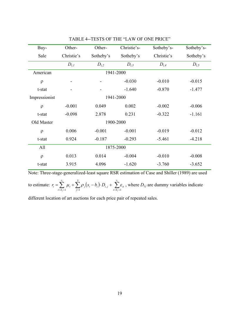
19

TABLE 4--TESTS OF THE “LAW OF ONE PRICE”

Buy-

Sale

Other-

Christie’s

Other-

Sotheby’s

Christie’s-

Sotheby’s

Sotheby’s-

Christie’s

Sotheby’s-

Sotheby’s

Di,1 Di,2 Di,3 Di,4 Di,5

American 1941-2000

ρ - - -0.030 -0.010 -0.015

t-stat - - -1.640 -0.870 -1.477

Impressionist 1941-2000

ρ -0.001 0.049 0.002 -0.002 -0.006

t-stat -0.098 2.878 0.231 -0.322 -1.161

Old Master 1900-2000

ρ 0.006 -0.001 -0.001 -0.019 -0.012

t-stat 0.924 -0.187 -0.293 -5.461 -4.218

All 1875-2000

ρ 0.013 0.014 -0.004 -0.010 -0.008

t-stat 3.915 4.096 -1.620 -3.760 -3.652

Note: Three-stage-generalized-least square RSR estimation of Case and Shiller (1989) are used

to estimate: ( ) ∑∑ ∑+=+= =

+⋅−+=i

i

i

i

s

btitjiii

s

bt jjti Dbsr

1,

1

5

1ερµ , where Di,j are dummy variables indicate

different location of art auctions for each price pair of repeated sales.

20

FIGURE 1: NUMBER OF OBSERVATIONS BY PURCHASE AND BY SALE

Note: For convenience, we will call the first price from each price pair “purchase price” and the

second price “sale price” from the perspective of the collector for the time period between the

two transactions of the price pair.

0

50

100

150

200

250

300

350

400

450

1875 1885 1895 1905 1915 1925 1935 1945 1955 1965 1975 1985 1995

Obs

erva

tions

PurchaseSale

21

FIGURE 2: NOMINAL INDICES

(Base Year: All 1875=1, American 1941=1, Impressionist 1941=1, Old Master 1900=1)

Notes: For the All Art Index, regression statistics for the three-stage-generalized-least square

RSR estimation of Case and Shiller: R2=0.64, F(125,4771) =104.32 with a significance level

equal to 0.000. Annual returns are computed as exp(µt + σ2/2)-1, σ2 is estimated in the second

stage of RSR.

0.1

1

10

100

1000

10000

100000

1875 1885 1895 1905 1915 1925 1935 1945 1955 1965 1975 1985 1995

ALLAmericanImpressionistOld Master

22

FIGURE 3: OLD MASTER PAINTINGS RESALE RETURNS

-60%

-40%

-20%

0%

20%

40%

60%

80%

$1 $10 $100 $1,000 $10,000 $100,000 $1,000,000 $10,000,000

PURCHASE PRICE

23

TABLE A1: NUMERICAL VALUES OF THE ALL ART INDEX

YEAR INDEX YEAR INDEX YEAR INDEX YEAR INDEX 1875 1.000 1907 7.264 1939 16.826 1971 412.032 1876 0.996 1908 9.590 1940 14.295 1972 487.115 1877 2.197 1909 5.323 1941 22.538 1973 713.655 1878 4.223 1910 8.283 1942 20.263 1974 591.168 1879 3.551 1911 17.153 1943 22.924 1975 479.239 1880 1.276 1912 13.205 1944 29.746 1976 690.213 1881 1.127 1913 16.790 1945 21.311 1977 725.746 1882 0.330 1914 12.023 1946 24.105 1978 873.930 1883 0.771 1915 11.050 1947 21.213 1979 1038.362 1884 0.469 1916 16.145 1948 19.227 1980 1462.642 1885 0.801 1917 25.759 1949 16.305 1981 1605.836 1886 1.293 1918 32.117 1950 19.502 1982 1536.404 1887 2.968 1919 16.397 1951 22.334 1983 1709.575 1888 1.408 1920 11.061 1952 29.365 1984 2014.648 1889 3.744 1921 5.346 1953 39.933 1985 2850.073 1890 4.151 1922 10.105 1954 27.782 1986 2738.594 1891 2.828 1923 19.283 1955 36.741 1987 3930.414 1892 2.247 1924 10.116 1956 59.051 1988 6290.526 1893 2.835 1925 11.365 1957 55.351 1989 7893.540 1894 1.782 1926 11.702 1958 67.850 1990 8640.364 1895 3.302 1927 12.535 1959 87.462 1991 5508.788 1896 1.256 1928 17.678 1960 78.351 1992 6452.997 1897 1.839 1929 10.916 1961 127.345 1993 5927.157 1898 3.050 1930 12.370 1962 132.238 1994 5360.433 1899 2.046 1931 9.775 1963 130.569 1995 7103.906 1900 2.546 1932 4.599 1964 152.155 1996 7705.580 1901 2.484 1933 7.402 1965 166.068 1997 6582.698 1902 3.529 1934 7.009 1966 192.539 1998 7810.311 1903 5.795 1935 10.793 1967 188.614 1999 8728.947 1904 2.616 1936 8.933 1968 266.613 1905 9.473 1937 6.311 1969 358.526 1906 4.449 1938 14.030 1970 285.117