DI

SC

US

SI

ON

P

AP

ER

S

ER

IE

S

Forschungsinstitut zur Zukunft der ArbeitInstitute for the Study of Labor

Preferences for Consistency

IZA DP No. 5840

July 2011

Armin FalkFlorian Zimmermann

Preferences for Consistency

Armin Falk University of Bonn,

CEPR, CESifo, DIW, MPI and IZA

Florian Zimmermann University of Bonn

Discussion Paper No. 5840 July 2011

IZA

P.O. Box 7240 53072 Bonn

Germany

Phone: +49-228-3894-0 Fax: +49-228-3894-180

E-mail: iza@iza.org

Any opinions expressed here are those of the author(s) and not those of IZA. Research published in this series may include views on policy, but the institute itself takes no institutional policy positions. The Institute for the Study of Labor (IZA) in Bonn is a local and virtual international research center and a place of communication between science, politics and business. IZA is an independent nonprofit organization supported by Deutsche Post Foundation. The center is associated with the University of Bonn and offers a stimulating research environment through its international network, workshops and conferences, data service, project support, research visits and doctoral program. IZA engages in (i) original and internationally competitive research in all fields of labor economics, (ii) development of policy concepts, and (iii) dissemination of research results and concepts to the interested public. IZA Discussion Papers often represent preliminary work and are circulated to encourage discussion. Citation of such a paper should account for its provisional character. A revised version may be available directly from the author.

IZA Discussion Paper No. 5840 July 2011

ABSTRACT

Preferences for Consistency* This paper studies how a preference for consistency can affect economic decision-making. We propose a two-period model where people have a preference for consistency because consistent behavior allows them to signal personal and intellectual strength. We then present three experiments that study main predictions and implications of the model. The first is a simple principal-agent experiment that shows that consistency is valued by others and that this value is anticipated. The second experiment underlines the crucial role of early commitment for consistency preferences. Finally we show how preferences for consistency can be used to manipulate choices. JEL Classification: C91, D03, D64 Keywords: consistency preferences, experiments, early commitment, charitable giving,

social influence Corresponding author: Armin Falk University of Bonn Adenauerallee 24 53113 Bonn Germany E-mail: armin.falk@uni-bonn.de

* We thank Roland Bénabou, Edward Glaeser, Uri Gneezy, Daniel Krähmer, Benny Moldovanu, Joel Sobel, Dezsö Szalay and Jean Tirole for helpful discussions. Valuable comments were also received from seminar participants at University of California - San Diego, Columbia University, Harvard University, University of Mannheim, Princeton University and Stockholm University. Financial support from the European Research Council (starting grant) is gratefully acknowledged.

1 Introduction

The desire to be and appear consistent is a powerful determinant of human behavior.

Once we have made a decision or taken a stand, we often experience pressure to live up

to that commitment. In this paper, we develop a simple model that specifies motives and

conditions that lead to consistent behavior. This allows predicting the role of consistency

in different decision contexts. Moreover, we provide results from three experiments and a

survey study that test the main predictions and implications of the model and underscore

the behavioral importance of consistency preferences.

Our model is built on the notion that consistent behavior is associated with “personal

and intellectual strength” (Cialdini, 1984). Evidence from social psychology suggests that

while consistency signals positive personality traits, inconsistent behavior is generally

associated with undesirable personal characteristics (see Asch, 1956 or Allgeier, Byrne,

Brooks and Revnes, 1979). Inconsistent beliefs, words or deeds are often indicative of

confusion or even mental illness. In the model decision-makers signal positive traits

when acting consistently. There are two types of decision-makers who repeatedly face

the same choice problem. Types with high personal and intellectual strength perfectly

know their preferred outcome while types with low strength are uncertain about it. Before

making a decision, low strength types receive noisy signals about their preferred outcome.

Regarding behavior over time, high strength types make consistent choices. However, the

beliefs, and consequently the choices, of low strength types can be inconsistent. Thus

personal and intellectual strength is associated with consistent choices.

We assume that decision-makers’ utility consists of two parts, a “standard” part

reflecting material concerns and a reputational part capturing decision-makers’ image

concerns for strength. This creates a trade-off between choosing according to updated

beliefs and reputational concerns. We show the existence of a Perfect Bayesian Equilib-

rium where decision-makers display preferences for consistency because consistent behav-

ior allows them to signal high personal and intellectual strength. The model allows for

several interpretations. The value of signaling can be interpreted as hedonic, i.e., peo-

ple like it if others think positively about them, or as strategic in the sense that people

expect benefits from future interactions, e.g., in the labor market. Depending on the

context signaling of strength is related to ability and knowledge, identity and personality

or predictability and reliability. Finally, the recipient of the signal can be others but also

the decision-maker himself. In this case the decision-maker learns about her own type by

observing and inferring from her own behavior (e.g., as in Benabou and Tirole, 2004 and

2

2006).

In the second part of the paper we report evidence from three decision experiments

and a survey study. The first experiment tests the basic logic of our model in a simple

principal-agent framework. We address two questions: do principals value consistency of

agents and is this value anticipated by agents? In the experiment the decision context is

a simple estimation task. Principals receive information about the estimation behavior of

two agents and need to select one for an additional estimation task. We find that agents

who estimate more consistently have a significantly higher chance of being selected by

principals. Anticipating the value of consistency, agents’ estimates in this treatment are

more consistent than in a control treatment where we eliminated the strategic value of

consistency.

The second experiment studies the role of early commitment for the preference for

consistency. Intuitively, actively committing to an opinion, belief, intention or action is

a precondition for observing consistent or inconsistent behavior. Without commitment,

i.e., without taking a stand or an action, possible inconsistencies are impossible to detect.

In a simple estimation context subjects have to perform an estimation task and receive

valuable information regarding the solution of the task. In the main treatment, subjects

commit to a first estimate prior to receiving the helpful information and without knowing

that they will later receive it. After they have received this information they are free to

revise their first estimate. In the control treatment, no prior commitment is made. We

find that the deviation of the final estimate from the valuable information is significantly

higher in the main treatment than in the control treatment. Prior commitment makes

subjects neglect valuable information leading to lower payoffs.

In the third experiment we examine the role of consistency preferences as a means

of social influence. The trick is to “tempt” a person to make a biased statement. In a

second step she is confronted with a request related to that statement and the pressure

to live up to it. Provided that the first statement involves little to no cost, it is relatively

easy to provoke biased statements. The preference for consistency will make the person

want to live up to the biased statement and act against her actual interest. We test this

prediction in the context of pro-social decision-making. We find that pro-social behavior

in the presence of biased statements systematically differs from behavior in a control

treatment where no first statements were made. Finally, in our survey study we show

how the preference for consistency can be used to manipulate subjects’ responses on a

particular matter, simply by adding an additional related question to the survey.

3

Our work is related to a literature in social psychology. Cialdini (1984) summarizes

much of the evidence and discusses several explanations for consistent behavior. In partic-

ular he highlights the role of consistency as a signal of positive attitudes. An alternative

interpretation of consistent choices relies on the notion of cognitive dissonance. This

approach basically assumes that consistent behavior reflects a desire to avoid cognitive

dissonances. Early work in this direction was developed in Heider (1946), Newcomb

(1953) and Festinger (1957).1 Another potential driver of consistent behavior is based on

the idea that thinking is not costless. If thinking does involve cognitive costs, it may in

fact be optimal to stick to a particular behavioral strategy and not to change behavior in

response to new information or new signals. It is likely that these motives all play some

role and often act in concert. Note, however, that neither cognitive dissonance nor cost of

thinking are sufficient to explain all results of our experiments. In particular, treatment

differences in our first experiment (repeated estimations with and without the presence

of a principal) can be explained in terms of our model and the notion that consistency

signals strength. However, neither cognitive dissonance nor cost of thinking would predict

any treatment difference.

Note that our notion of consistency is conceptually different from anchoring effects. In

a classical anchoring experiment, Tversky and Kahneman (1974) for example generated a

random number between 0 and 100 and asked subjects if the number of African nations in

the United Nations was greater than that number. Then they asked subjects to estimate

the number of African nations in the United Nations. They find that the randomly

generated number (the anchor) significantly affected estimates. Studies on anchoring

manipulations differ from the notion of consistency in that they document effects of

random unrelated numbers on subsequent choices. In our paper, subsequent choices are

affected by prior actions or statements. In addition the role of reputation stressed in

our model is not present in work on anchoring effects, which also implies that anchoring

effects cannot explain our experimental findings.

In the economics literature Eyster (2002) and Yariv (2005) have suggested models of

consistent behavior. In Eyster (2002) people have a taste for rationalizing past mistakes

by taking current actions that justify these mistakes. His model offers an explanation

for the well-known “sunk-cost effect”. It also predicts procrastination in search contexts

and overbidding in wars of attrition. Yariv (2005) proposes a model where people have a

1Akerlof and Dickens (1982) incorporate cognitive dissonance theory into an economic model. In anempirical study, Mullainathan and Washington (2009) examine the consequences of cognitive dissonancein the context of voting behavior.

4

taste for consistency of beliefs held over time, thereby reducing cognitive dissonance. Her

model can explain a variety of phenomena such as underpinnings of overconfidence and

underconfidence, persistence of actions over time or why people sometimes might prefer

to receive less accurate information. Different to our approach, Eyster (2002) and Yariv

(2005) directly assume a taste for consistency while in our model this taste results from a

desire to signal strength. Also, their models focus on internal consistency while our model

stresses the role of reputation for consistency preferences. Ellingsen and Johannesson

(2004) and Vanberg (2008) refer to the taste for consistency as a possible reason for why

people incur costs of lying and thus keep their promises. In fact, breaking promises can

be viewed as a particularly obvious form of inconsistency. On a more general level, our

model belongs to a class of models where decision-makers try to signal positive traits

through their actions (as for example in Bernheim, 1994, Prendergast and Stole, 1996,

Benabou and Tirole, 2006, Ellingsen and Johannesson, 2008 or Andreoni and Bernheim,

2009).

The remainder of the paper is organized as follows: In the next section we introduce

our model. In section 3 we present the three experiments and our survey study. Section 4

concludes and discusses several implications of our work for, e.g., the design of committee

procedures or problems of self-control.

2 The Model

We model the intuition that “... a high degree of consistency is normally associated

with personal and intellectual strength.” (Cialdini, 1984). We choose a very simple set-

up with two types of decision-makers who choose between two alternatives. The model

formalizes the notion of preferences for consistency and delivers behavioral predictions

for our experiments.2

2.1 Set-up

There are two periods, t = 1, 2. In both periods, a decision-maker (D) chooses xt from

a choice set X = {Red,Blue} in public. D has a preferred outcome µ ∈ X. There

are two different types of decision-makers. Types with high personal and intellectual

strength (type DH) perfectly know their preferred outcome µ. Types with low personal

2We have also developed an alternative and more general version of the model with a continuous typeand choice set. Insights and predictions of this model are qualitatively similar to the more parsimoniousset-up. We therefore decided to use the latter. The continuous version is available on request.

5

and intellectual strength (type DL) are uncertain about their preferred outcome. Her

type is D’s private knowledge but is commonly known to be drawn from a distribution

with probability α that D is of type DH and (1− α) that she is of type DL. Types with

low strength and the public are holding an uninformative prior on µ, i.e., Pr(µ = Red) =

Pr(µ = Blue) = 12. In both periods, before making a choice, DL privately receives a

signal mt about µ. Signals are of strength pt, i.e., pt = Pr(mt = Red|µ = Red) =

Pr(mt = Blue|µ = Blue). We assume that signals are informative with 12< pt < 1. We

allow that the strength of signals differs between periods 1 and 2, only requiring that

p2 ≥ p1. Thus our setup captures situations where the quality of information DL receives

may change over periods. The assumption that signals in period 2 are at least as strong

as signals in period 1 is only made to focus on scenarios where contradicting signals lead

to changes in beliefs about the preferred outcome.3

Upon receiving a signalmt, DL updates beliefs about µ following Bayes’ rule. Through-

out the paper l(mt,mt−1) denotes DL’s beliefs about µ in terms of the probability she

assigns on Red being her preferred outcome conditional on signals mt and mt−1 (if mt−1

exists), i.e., l(mt,mt−1) = Pr(µ = Red|mt,mt−1).

Since the prior on µ is uninformative, DL’s updated period 1 belief is determined by

the signal she received in period 1, m1. Accordingly, the updated belief on µ in period 1

is l(m1 = Red) = p1 >12

and l(m1 = Blue) = (1− p1) < 12, respectively. In period 2, DL

receives an additional signal m2 and updates again. Thus:

(1) l(m2 = Red,m1 = Red) =p1 ∗ p2

p1 ∗ p2 + (1− p1)(1− p2)>

1

2

(2) l(m2 = Blue,m1 = Red) =p1 ∗ (1− p2)

p1 ∗ (1− p2) + (1− p1) ∗ p2≤ 1

2

(3) l(m2 = Blue,m1 = Blue) = 1− p1 ∗ p2p1 ∗ p2 + (1− p1)(1− p2)

<1

2

(4) l(m2 = Red,m1 = Blue) = 1− p1 ∗ (1− p2)p1 ∗ (1− p2) + (1− p1) ∗ p2

≥ 1

2

In both periods, the decision-maker chooses xt in order to maximize utility. D’s

utility function consists of two components. The first is “standard” outcome-based utility.

Standard utility is 1 if D chooses xt = µ and 0 otherwise. The decision-maker also cares

about her reputation. She likes it, if the public perceives her as having high personal

3If the period 2 signal is less informative than the period 1 signal, updated period 2 beliefs alwaysremain in line with the signal from period 1 even in case of contradicting signals. Consequently typesDL would always choose consistently anyway.

6

and intellectual strength. An alternative interpretation of the reputational concern is a

desire for a positive self-image (similar as in Benabou and Tirole, 2004 and 2006). In this

case decision-makers receive a perfect signal about their personal and intellectual strength

prior to their decision. Thus, when deciding, they know their strength. However, for their

self-assessment, this knowledge is not readily available, e.g., due to reasons of imperfect

recall. Since actions are easier to recall than signals, decision-makers use past actions for

their self-assessment. Thus the model is compatible with the intuition that people care

about their self-image and construct self-image from past actions. In the following we

describe the model mostly in terms of public reputation but always mean to include a

self-signaling interpretation. Reputational concerns are expressed by

−β ∗ Pr(type = DL|xt, xt−1).

P r(type = DL|xt, xt−1) denotes the public’s (or D’s) belief about D’s type, condi-

tional on D’s decisions in the current period xt and the previous period xt−1 (if it exists).

Parameter β is assumed to be positive and specifies how much D cares about her repu-

tation. Differences in β might reflect, e.g., the size and importance of the public or the

social distance between D and the public. The nature of reputational concerns could be

strategic in the sense that people expect benefits in future interactions. In labor relations,

e.g., signaling higher abilities may improve hiring prospects or lead to higher wages and

promotion. Alternatively, β could reflect a hedonic value of reputation. People simply

enjoy being regarded as intellectually and personally strong. Depending on the context,

personal and intellectual strength is associated with different personal characteristics. In

task-related choices, similar solutions to similar problems signal high ability. In repeated

social interactions, personal and intellectual strength, reflected by consistent behavior,

signals predictability and reliability. These are important prerequisites for relationship

formation and trust (see Brown, Falk and Fehr, 2004). They also help solving coordina-

tion problems. High personal and intellectual strength is also a sign of personal identity.

Identity is shaped by past actions or statements. Without continuity in actions or state-

ments, the formation of a sense of self-identity is not possible. In that sense, high personal

and intellectual strength (via consistent behavior over time) is a prerequisite for strong

personal identity.

Putting these two components together, in periods 1 and 2 DL’s expected utility is

given by

7

E(Ut(xt)) =

l(mt,mt−1) ∗ 1− β ∗ Pr(type = DL|xt, xt−1) if xt = Red

(1− l(mt,mt−1)) ∗ 1− β ∗ Pr(type = DL|xt, xt−1) if xt = Blue.

In periods 1 and 2, DL maximizes E(Ut) facing a trade-off between maximizing

outcome-based utility and gaining reputation.4

Note that we assume myopic, non-forward looking behavior. Decision-makers are not

anticipating period 2 decisions when deciding in period 1. This can be justified in two

ways. First, we are interested in situations where future decisions are not anticipated

and believe that this is quite common. Second, and more importantly, predicted be-

havior is actually identical if decision-makers are forward looking. The reason is that

choosing according to their beliefs in period 1 is optimal not only from a standard utility

perspective. It also maximizes the likelihood of consistent behavior. It is therefore not

possible to improve in terms of consistency even in situations where the decision-maker

anticipates future decisions.

2.2 Equilibrium

We now turn to equilibrium behavior. In period 1 the equilibrium we consider is straight-

forward. D always maximizes standard utility. Types DL choose x∗1 = Red if m1 = Red

and x∗1 = Blue if m1 = Blue. Types DH choose their preferred outcome µ. Due

to the uninformative prior of the public, D cannot affect her image through x1, i.e.,

Pr(type = DL|x1 = Red) = Pr(type = DL|x1 = Blue). Thus simply maximizing stan-

dard utility is optimal and the behavior described above constitutes a Perfect Bayesian

Equilibrium.5

In period 2 there now exists a choice history x∗1 and D faces a possible trade-off

between standard utility and reputational concerns. We characterize the equilibrium

conditional on x∗1. To simplify notation we consider the case where x∗1 = Red without

loss of generality.

4Utility of the high types is straightforward. Suppose a type DL with µ = Red. Her utility is described

by Ut(xt) =

{1− β ∗ Pr(type = DL|xt, xt−1) if xt = Red

0− β ∗ Pr(type = DL|xt, xt−1) if xt = Blue.5As is common for this type of signaling models, there exist other equilibria. For example, if repu-

tational concerns are large enough, there exists a Perfect Bayesian Equilibrium where D always choosesRed (or Blue) regardless of her beliefs about µ and her type and the public holds off-equilibrium beliefsthat D is a low type, i.e., Pr(type = DL|Blue) = 1 (or Pr(type = DL|Red) = 1).

8

Types DH who chose Red in period 1 know with certainty that their preferred outcome

is Red. For types DL who chose Red in period 1 we need to distinguish two possibilities.

In period 2 they either receive a signal m2 = Red or m2 = Blue. In the first case we have

that l(m2 = Red,m1 = Red) > 12, in the second case l(m2 = Blue,m1 = Red) ≤ 1

2. If D

would simply maximize standard utility, types DH and types DL with m2 = Red would

choose x2 = Red whereas types DL with m2 = Blue would choose x2 = Blue.6 In the

presence of image concerns however, DL types with contradicting signals face a trade-off

between maximizing standard utility and signaling personal and intellectual strength.

We show under which conditions there exists a Perfect Bayesian Equilibrium in period 2

where types with low strength and contradicting signals nevertheless choose consistently,

thereby sacrificing expected standard utility.

In the equilibrium, types DH , types DL with signals m2 = Red,m1 = Red and types

DL with signals m2 = Blue,m1 = Red all behave consistently choosing Red in period 2.

For this to be an equilibrium it suffices to check incentive compatibility for low strength

types with contradicting signals. If incentive compatibility is fulfilled for these types it

is straightforward that for types DH and types DL with signals m2 = Red,m1 = Red it

is fulfilled as well. Decision-makers DL with signals m2 = Blue,m1 = Red hold beliefs

l(m2 = Blue,m1 = Red) ≤ 12. We need to check that they are better off choosing

Red than choosing Blue. Standard utility is l(m2 = Blue,m1 = Red) ∗ 1 when they

choose Red and (1− l(m2 = Blue,m1 = Red)) ∗ 1 when they choose Blue. Reputational

utility is −β ∗ Pr(type = DL|Red,Red) = −β ∗ (1 − α) if they choose consistently and

−β ∗Pr(type = DL|Blue,Red) = −β if they choose inconsistently.7 We end up with the

following condition: DL’s with contradicting signals prefer Red over Blue if

α ∗ β ≥ 1− 2 ∗ l(m2 = Blue,m1 = Red).

The above condition captures the trade-off between standard utility and reputational

concerns. The left hand side describes reputational gains from choosing consistently while

the right hand side represents the costs in terms of standard utility. If image concerns are

sufficiently high, decision-makers display a preference for consistency because consistent

6If signals in periods 1 and 2 are of equal strength, DL’s with contradicting signals are indifferent interms of standard utility between Red and Blue.

7Note that we assume off-equilibrium beliefs such that the public infers low personal and intellectualstrength from inconsistent behavior. We believe that this assumption is plausible. High types knowtheir preferred outcome with certainty. Consequently they have the highest expected costs in terms ofstandard utility from choosing inconsistently. Also, if only a small fraction of decision-makers wouldnot have any reputational concerns and only maximize standard utility, only low types would chooseinconsistently. In addition, our equilibrium satisfies the Intuitive Criterion (Cho and Kreps, 1987).

9

behavior allows them to signal personal and intellectual strength. Note that if reputa-

tional concerns are small, there exists an equilibrium in period 2 where D always chooses

to maximize standard utility. We summarize this result in the following proposition.

PROPOSITION 1: Assume w.l.g. that x∗1 = Red. If reputational concerns β are

sufficiently large, i.e., α ∗ β ≥ 1− 2 ∗ l(m2 = Blue,m1 = Red), there exists a Perfect

Bayesian Equilibrium in period 2, where D always chooses x∗2 = x∗1 = Red.

Proposition 1 states the main result of our model, namely, that decision-makers have

a preference for consistent behavior. In period 2, decision-makers do not simply maximize

standard outcome-based utility. Instead, they act consistently with their period 1 choice

in order to signal high personal and intellectual strength. Thus, in equilibrium, they are

willing to sacrifice outcome-based utility to increase their reputational utility.

3 Experimental Evidence

In this section we present evidence from three experiments designed to test the basic

logic of the model and to examine different applications of preferences for consistency. In

particular we address the following issues: First, we study the signal value of consistent

behavior in the context of a simple principal agent game. In the second experiment we

investigate the role of commitment. The idea is that without explicit commitment to

some point of view, statement or intention, inconsistencies are impossible to detect and

consequently costs of inconsistency are less important. Our third experiment demon-

strates the importance of consistency preferences for social influence and manipulation.

In addition, we present evidence from a study that shows how the taste for consistency

can be used to manipulate survey answers.8

3.1 Experiment 1: The Value of Consistency

Design: The first experiment tests the central assumption of the model, that consistent

behavior is valued. In the experiment the decision context involves a simple estimation

task. We test whether principals infer higher ability from more consistent estimates and

whether agents anticipate this.

8Instructions for the three experiments and the complete survey can be found in Appendix C.

10

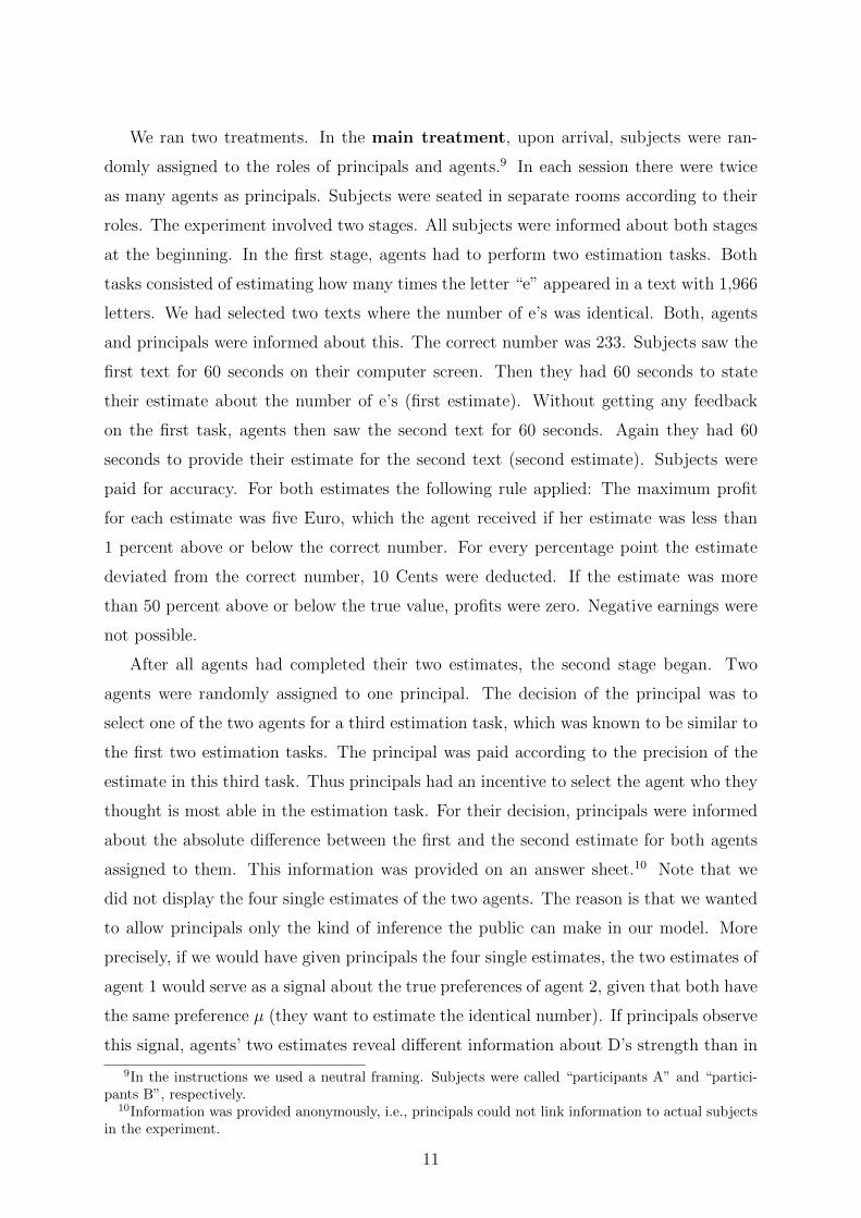
We ran two treatments. In the main treatment, upon arrival, subjects were ran-

domly assigned to the roles of principals and agents.9 In each session there were twice

as many agents as principals. Subjects were seated in separate rooms according to their

roles. The experiment involved two stages. All subjects were informed about both stages

at the beginning. In the first stage, agents had to perform two estimation tasks. Both

tasks consisted of estimating how many times the letter “e” appeared in a text with 1,966

letters. We had selected two texts where the number of e’s was identical. Both, agents

and principals were informed about this. The correct number was 233. Subjects saw the

first text for 60 seconds on their computer screen. Then they had 60 seconds to state

their estimate about the number of e’s (first estimate). Without getting any feedback

on the first task, agents then saw the second text for 60 seconds. Again they had 60

seconds to provide their estimate for the second text (second estimate). Subjects were

paid for accuracy. For both estimates the following rule applied: The maximum profit

for each estimate was five Euro, which the agent received if her estimate was less than

1 percent above or below the correct number. For every percentage point the estimate

deviated from the correct number, 10 Cents were deducted. If the estimate was more

than 50 percent above or below the true value, profits were zero. Negative earnings were

not possible.

After all agents had completed their two estimates, the second stage began. Two

agents were randomly assigned to one principal. The decision of the principal was to

select one of the two agents for a third estimation task, which was known to be similar to

the first two estimation tasks. The principal was paid according to the precision of the

estimate in this third task. Thus principals had an incentive to select the agent who they

thought is most able in the estimation task. For their decision, principals were informed

about the absolute difference between the first and the second estimate for both agents

assigned to them. This information was provided on an answer sheet.10 Note that we

did not display the four single estimates of the two agents. The reason is that we wanted

to allow principals only the kind of inference the public can make in our model. More

precisely, if we would have given principals the four single estimates, the two estimates of

agent 1 would serve as a signal about the true preferences of agent 2, given that both have

the same preference µ (they want to estimate the identical number). If principals observe

this signal, agents’ two estimates reveal different information about D’s strength than in

9In the instructions we used a neutral framing. Subjects were called “participants A” and “partici-pants B”, respectively.

10Information was provided anonymously, i.e., principals could not link information to actual subjectsin the experiment.

11

the absence of that knowledge. Therefore we decided only to provide absolute differences

between estimates to the principals, thereby only allowing the kind of inference on D’s

strength that is assumed in our model.

On their answer sheet principals had to select “their” agent. The third task was to

estimate how many times the letter “a” appears in a text of again 1966 letters. Principals

were paid according to the accuracy of the selected agent’s third estimate. The maximum

payoff was ten Euro, which was paid if the agent’s estimate was less than 1 percent above

or below the correct number. For every percentage point the estimate deviated from the

correct number, 20 Cents were deducted. If the estimate was more than 50 percent above

or below the correct value, principal’s payoff was zero. Agents had an incentive to be

selected and to estimate as precise as possible in the third task. They received a prize of

10 Euro for being selected. In addition, they were paid according to accuracy identically

to the payment scheme in the first two estimates.

Principals’ selection decisions inform us about the potential value of estimating con-

sistently. However, to examine whether agents anticipate this value and actually behave

more consistently we need an additional treatment that eliminates (or reduces) the im-

portance of reputational concerns for consistency. This is what we do in the control

treatment. The control treatment was simply the first stage of the main treatment, i.e.,

agents estimate how many times the letter “e” appeared in the two texts used in the

main treatment. The payoff scheme for the two tasks was identical to that of the main

treatment. Comparing behavior between the two treatments informs us whether agents

anticipate the value of consistency and therefore behave more consistently in the main

treatment.

Procedural Details: A total of 168 subjects participated in six sessions. In the

main treatment, 64 subjects participated as agents and 32 as principals. 72 subjects

participated in the control treatment. Subjects were mostly students from various fields

at the University of Bonn and were recruited using the online recruitment system by

Greiner (2003). No subject participated in more than one session. The experiment was

run using the experimental software z-Tree (Fischbacher, 2007). The principals made

their choice on an answer sheet. Sessions lasted on average about 60 minutes in the main

treatment and 45 minutes in the control treatment. Average earnings were 12.90 Euro for

principals and 12.06 Euro for agents, including a show-up fee of eight Euro for principals

and four Euro for agents.11

11One Euro was worth about 1.35 U.S. dollar at the time.

12

Hypotheses: Principals value consistent behavior. They infer high ability from

consistent estimates. Thus agents who estimate more consistently should have a higher

probability of being selected by principals. In our model the value of consistency is ex-

pressed as an increase in the reputational concern β. While reputational concerns in

the control treatment (βc) are not necessarily zero (e.g., due to self-signaling motives),

reputational concerns in the main treatment (βm) are higher, i.e., βm > βc. This follows

simply from the strategic value of reputation for high ability. In the main treatment we

implemented a tournament incentive structure where agents win a prize if they outper-

form the other agent. These tournament incentives lead to a strategic value of behaving

consistently that is not present in the control treatment. A higher β leads to greater

importance of the desire to be and appear consistent relative to the goal of maximizing

standard utility. Consequently, the likelihood of an equilibrium where all decision-makers

behave consistently is higher in the main treatment compared to the control treatment.

Proposition 1 states the condition under which an equilibrium where all decision-makers

act consistently exists: α ∗ β ≥ 1 − 2 ∗ l(m2 = Blue,m1 = Red). It can be easily seen

that an increase in β makes the fulfillment of this condition more likely.12 Our main

hypotheses can be summarized as follows:

HYPOTHESIS EXPERIMENT 1: (i) The likelihood that an agent is selected by a

principal decreases in the absolute difference between first and second estimate. (ii) The

absolute difference between first and second estimate is smaller in the main treatment

than in the control treatment.

Results: The first result concerns the selection decisions of principals. In line with

our hypothesis, a higher absolute difference between the two estimates decreases the

likelihood of being selected. Figure 1 shows that the likelihood of being selected is about

70 percent for differences between zero and five and declines for larger differences. For

differences larger than 31, e.g., the likelihood drops to about 22 percent. The decrease

in likelihood is significant as shown by a simple Probit regression. When we regress

the probability of being selected on the absolute differences between the estimates we

get a negative and significant coefficient (p-value <0.01). The marginal effect is -0.012,

indicating that an increase in the absolute difference by one point decreases the likelihood

of being selected by about 1.2 percent. Further evidence comes from the observation that

12The simplistic character of this prediction follows from the simple structure of our model. A moregeneral version of the model makes the prediction that an increase in reputational concerns should makeall decision-makers behave more consistently, leading to a shift in the distribution of distances betweenthe two estimates. This version with a continuous type and choice set is available upon request.

13

among all principals 75 percent select the agent with the smaller absolute difference. A

simple binomial test rejects the null hypothesis that principals randomized with equal

probability (p-value <0.01).

0.3

0.4

0.5

0.6

0.7

0.8

Pro

babi

lity

of B

eing

Sel

ecte

d

0

0.1

0.2

[0-5] [6-15] [16-30] [31- ]

Pro

babi

lity

of B

eing

Sel

ecte

d

Absolute Difference Between Estimates

Figure 1: Probability of being selected by principal dependent on the absolute difference between twoestimates.

We now turn to agents’ behavior. The correct answer for both estimations was 233.

Using all estimates (main and control treatment), the average first estimate was 220.57

while the average second estimate was 215.64.13 The variance in estimates was rather

high. The standard deviation of all estimates in the first task was 83.29, in the second

it was 74.39. At the end of the experiment, we asked agents in the control treatment

to briefly describe their estimation strategy for the two estimation tasks.14 Almost all

decision-makers who answered the question described a similar procedure. First they

counted the number of e’s for a couple of rows. Then they counted the total amount of

rows in the text and projected the total number of e’s in the text.

Given principals’ behavior, the model predicts that agents choose more consistently

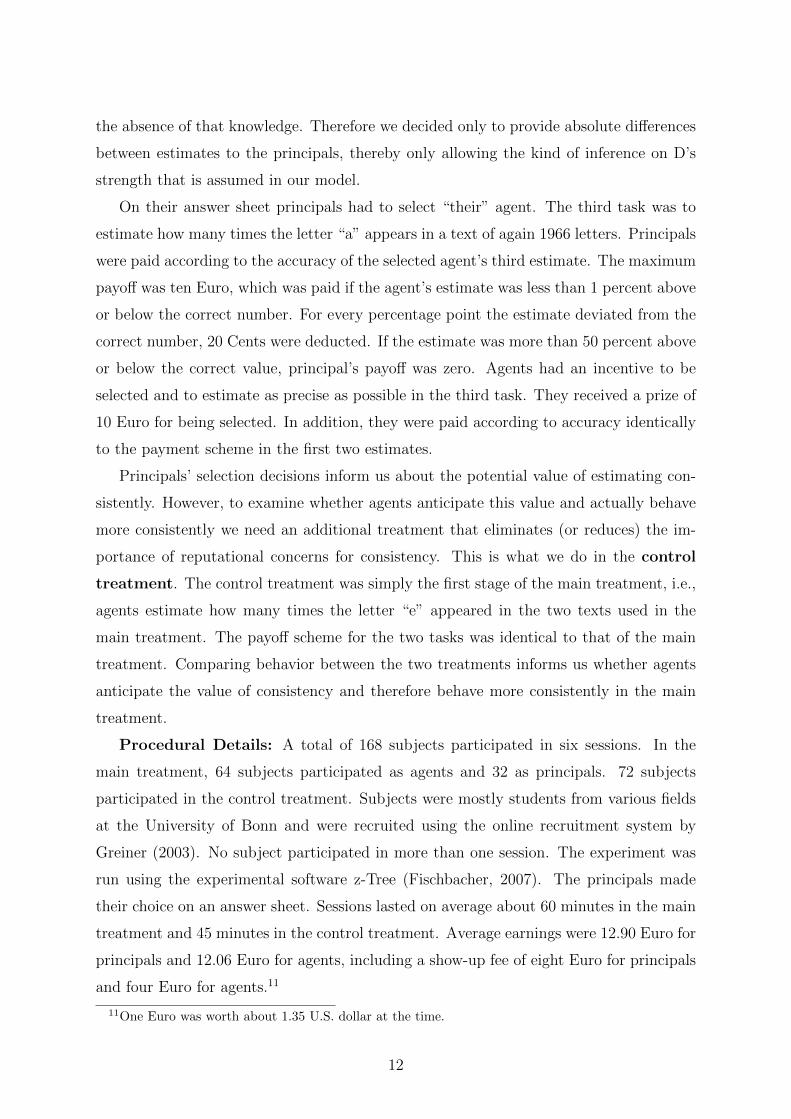
in the main than in the control treatment. This is in fact what we find. Figure 2

shows scatterplots of first and second estimates. The left panel displays observations

from the control treatment, the right panel from the main treatment. While estimates

are correlated in both treatments, the correlation is much tighter in the main treatment,

i.e., decisions are more consistent. The correlation coefficients are 0.37 in the control

13The result that the average estimate from a large population is close to the true value is also referredto as the “wisdom of the crowds” (see for example Surowiecki, 2004).

14The question we asked was the following: “Please briefly describe how you proceeded in the twoestimation tasks. How did you get to your estimation results?”

14

0

50

100

150

200

250

300

350

400

450

500

0 100 200 300 400 500

Est

imat

e 2

Estimate 1

Control Treatment

0

50

100

150

200

250

300

350

400

450

500

0 100 200 300 400 500

Est

imat

e 2

Estimate 1

Main Treatment

Figure 2: Scatterplots of first and second estimates for both treatments.

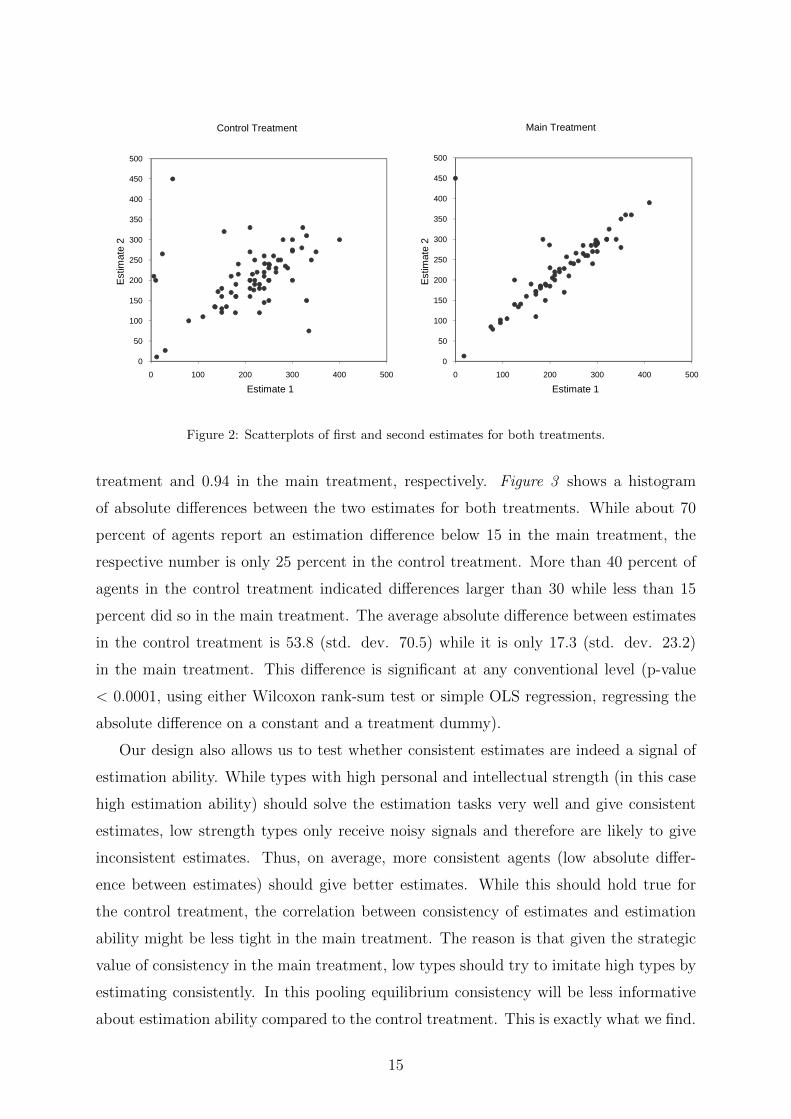
treatment and 0.94 in the main treatment, respectively. Figure 3 shows a histogram

of absolute differences between the two estimates for both treatments. While about 70

percent of agents report an estimation difference below 15 in the main treatment, the

respective number is only 25 percent in the control treatment. More than 40 percent of

agents in the control treatment indicated differences larger than 30 while less than 15

percent did so in the main treatment. The average absolute difference between estimates

in the control treatment is 53.8 (std. dev. 70.5) while it is only 17.3 (std. dev. 23.2)

in the main treatment. This difference is significant at any conventional level (p-value

< 0.0001, using either Wilcoxon rank-sum test or simple OLS regression, regressing the

absolute difference on a constant and a treatment dummy).

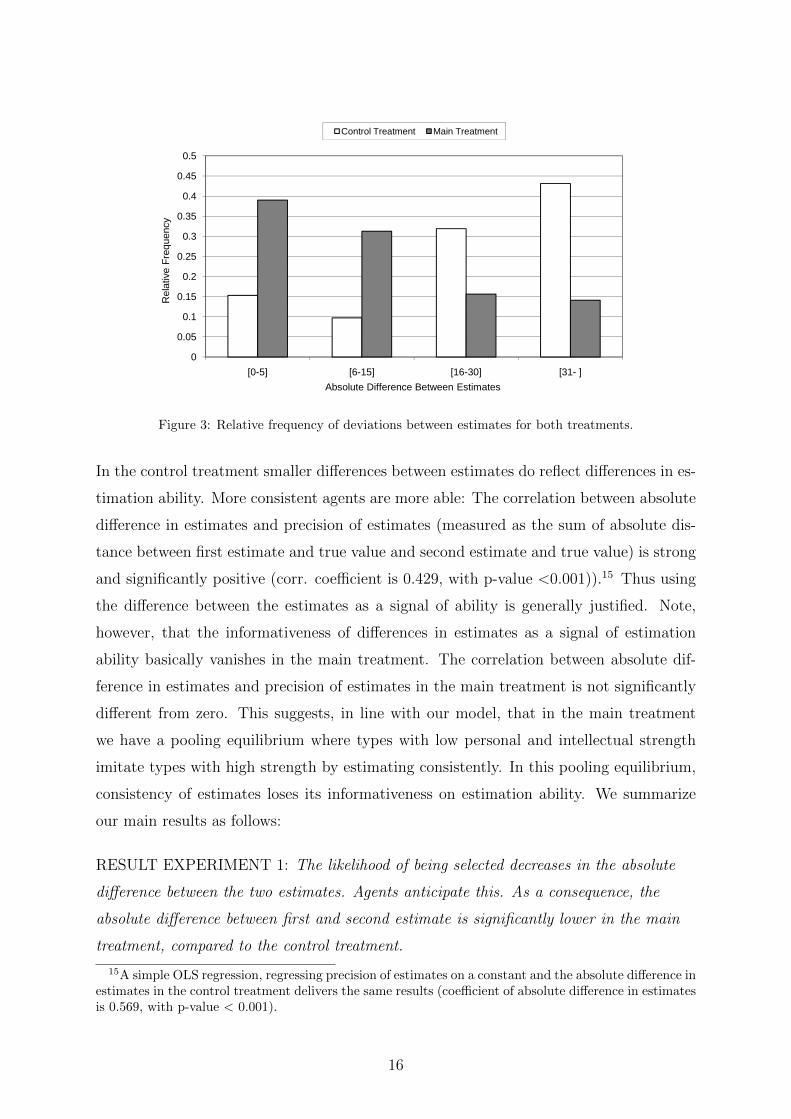
Our design also allows us to test whether consistent estimates are indeed a signal of

estimation ability. While types with high personal and intellectual strength (in this case

high estimation ability) should solve the estimation tasks very well and give consistent

estimates, low strength types only receive noisy signals and therefore are likely to give

inconsistent estimates. Thus, on average, more consistent agents (low absolute differ-

ence between estimates) should give better estimates. While this should hold true for

the control treatment, the correlation between consistency of estimates and estimation

ability might be less tight in the main treatment. The reason is that given the strategic

value of consistency in the main treatment, low types should try to imitate high types by

estimating consistently. In this pooling equilibrium consistency will be less informative

about estimation ability compared to the control treatment. This is exactly what we find.

15

0.2

0.25

0.3

0.35

0.4

0.45

0.5R

elat

ive

Fre

quen

cy

Control Treatment Main Treatment

0

0.05

0.1

0.15

[0-5] [6-15] [16-30] [31- ]

Rel

ativ

e F

requ

ency

Absolute Difference Between Estimates

Figure 3: Relative frequency of deviations between estimates for both treatments.

In the control treatment smaller differences between estimates do reflect differences in es-

timation ability. More consistent agents are more able: The correlation between absolute

difference in estimates and precision of estimates (measured as the sum of absolute dis-

tance between first estimate and true value and second estimate and true value) is strong

and significantly positive (corr. coefficient is 0.429, with p-value <0.001)).15 Thus using

the difference between the estimates as a signal of ability is generally justified. Note,

however, that the informativeness of differences in estimates as a signal of estimation

ability basically vanishes in the main treatment. The correlation between absolute dif-

ference in estimates and precision of estimates in the main treatment is not significantly

different from zero. This suggests, in line with our model, that in the main treatment

we have a pooling equilibrium where types with low personal and intellectual strength

imitate types with high strength by estimating consistently. In this pooling equilibrium,

consistency of estimates loses its informativeness on estimation ability. We summarize

our main results as follows:

RESULT EXPERIMENT 1: The likelihood of being selected decreases in the absolute

difference between the two estimates. Agents anticipate this. As a consequence, the

absolute difference between first and second estimate is significantly lower in the main

treatment, compared to the control treatment.

15A simple OLS regression, regressing precision of estimates on a constant and the absolute difference inestimates in the control treatment delivers the same results (coefficient of absolute difference in estimatesis 0.569, with p-value < 0.001).

16

3.2 Experiment 2: The Role of Commitment

Our second experiment studies the role of early commitment. Intuitively, actively com-

mitting to an opinion, belief, intention or action is a precondition for observing consistent

or inconsistent behaviors. Without commitment, i.e., without taking a stand or an action,

observers will not be able to detect possible inconsistencies. Therefore, a decision-maker

is not constrained by reputational concerns and can maximize utility without taking rep-

utational costs into account. In contrast, once an individual has committed to an opinion

or belief, she cannot easily change her mind without revealing some inconsistency. We

test this intuition and prediction of our model in the context of an estimation task and

show how commitment to an opinion can make people disregard valuable information.

Design: We study two treatments, one with commitment (main treatment) and

one without (control treatment). The different steps of the experiment are illustrated

in Figure 4. The main treatment is shown in the upper panel. First, subjects were

explained the task: Subjects had to estimate the number of peas in a bowl.16 Subjects

were paid according to the precision of their estimate. If their estimate was less than 5

percentage points above or below the true value of 3000, subjects earned 10 Euro. For

every 5 percentage points the estimate deviated from the true value, we deducted 50

Cents. For example, a subject whose estimate deviated 17 percent from the true value

earned 8.50 Euro. Negative earnings from the estimation task were not possible.

Subjects were seated around a table which was placed in the middle of the lab.17 After

subjects had been informed about the task the bowl was shown. The bowl with peas was

placed in the middle of the table. Subjects were asked to raise their hand once they had

written down their estimate on an answer sheet that had been distributed at the beginning

of the experiment. As soon as a subject indicated that he or she had written down an

estimate, the experimenter went to the subject and recorded the subject’s estimate. This

means that subjects had written down their first estimate and knew that the experimenter

knew this estimate. At this point, subjects had committed to their first estimate. After

all subjects had stated their estimates, the experimenter announced that he would now

provide subjects with additional and “helpful” information regarding the estimation task.

Each subject received an information sheet containing the following sentence. “In the

past it has often been the case in various estimation tasks, that the average estimate of all

participants is often relatively close to the true value. The estimation task you are facing

16A picture of the bowl is shown in Appendix A.17Subjects were seated sufficiently far away from each other, such that they could not see what other

subjects were writing down.

17

has also been conducted with a different group of participants. They have also been paid

according to precision of their estimates. The average estimate of the number of peas

in the bowl of this group was 2615. If you want to, you can now revise your estimate.”

After they received the information sheet, subjects had time to revise their estimate on

their answer sheet. Of course, only the final estimate was relevant for earnings. After

all subjects had indicated that they had specified their final estimate, the experimenter

collected their answer sheets and the estimation task ended.

Figure 4: Timing of the experiment

The additional information we provided to subjects was based on a separate experi-

ment we had conducted with 61 different subjects. They faced the same estimation task

and were also paid according to the precision of their estimates. The average estimate of

that group was 2615. In the results section we show that the additional information was

in fact valuable to subjects.

Subjects in the control treatment also learned about the task and were asked to

provide an estimate. The only difference between main and control treatment was that in

the latter subjects did not state an estimate prior to receiving the additional information

(see lower panel of Figure 4 ). In the control treatment, subjects saw the bowl with peas

for some time prior to receiving the information sheets.18 The time was approximated to

be the same as what subjects in the main treatment needed. During this time subjects

could form a belief about the correct number of peas, but did not state this to the

18Note that in both treatments subjects did not know that they would receive helpful informationbefore they actually received it.

18

experimenter, i.e., no commitment to a first estimate was made. After subjects received

the information sheets, they stated their estimate on their answer sheet. Answer sheets

were collected by the experimenter and the estimation task ended.

Procedural Details: A total of 54 subjects participated in four sessions, 28 in the

main and 26 in the control treatment. Subjects were mostly undergraduate students from

various fields at the University of Bonn and were recruited using the online recruitment

system by Greiner (2003). No subject participated in more than one session. The experi-

ment was conducted with paper and pencil. Sessions lasted on average about 40 minutes.

Subjects earned on average 12.31 Euro, including a show-up fee of 5 Euro.

Hypotheses: Here we present the intuition of our model’s prediction. A formal

prediction is derived in Appendix B. In both treatments subjects see the bowl and form a

belief about the correct number of peas. In the main treatment subjects commit to their

belief by stating it towards the experimenter. Then, in both treatments subjects receive

a public signal, i.e., valuable information. In the main treatment subjects necessarily

reveal inconsistency if they respond to the public signal by changing their final estimate

accordingly. On the contrary, subjects in the control treatment can respond to the public

signal without revealing inconsistency due to the lack of commitment to their prior belief.

Therefore the preference for consistency will make subjects partially neglect the valuable

information in the main treatment. Consequently final estimates in the main treatment

will be further away from the public signal than in the control treatment. Since subjects

in the main treatment disregard valuable information, it follows directly that the quality

of estimates and therefore earnings are lower in the main than in the control treatment.19

We summarize our hypothesis as follows:

HYPOTHESIS EXPERIMENT 2: The absolute difference between the final estimate

and the information value of 2615 should be higher in the main treatment, compared to

the control treatment. Final estimates in the main treatment will be further away from

the correct value of 3000 compared to the control treatment.

Results: Pooling data from both treatments the average (final) estimate was 2552.50.

The estimation problem is very difficult and answers ranged from 500 to 5800. Accord-

ingly, the variance was large as indicated by a standard deviation of 1021.87. We chose

19We abstract here from self-signaling motives. Subjects could signal strength towards themselvesby being consistent with their private belief. Since this motive is present in both treatments, it doesnot change our predictions. One might even argue that self-signaling should be stronger in the maintreatment. There private beliefs might be more salient for self-evaluation because they were actuallystated.

19

a difficult task on purpose as it offers an ideal context to provide subjects with helpful

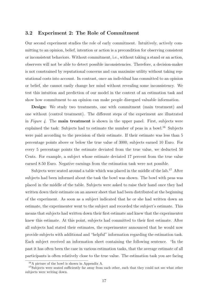
information. To show that the public signal was in fact valuable we simply count the

number of subjects in the main treatment whose estimate in the first estimation was

closer to 3000 than 2615. It turns out that this holds for only 5 out of 28 subjects. This

means that about 82 percent of subjects could improve their (first) estimate by simply

choosing 2615 or by moving in this direction.

0.1

0.15

0.2

0.25

0.3

Rel

ativ

e F

requ

ency

Control Treatment Main Treatment

0

0.05

0.1

[0- ] [1415- ] [1715- ] [2015- ] [2315- ] [2615- ] [2915- ] [3215- ] [3515- ] [3815- ]

Rel

ativ

e F

requ

ency

Final Estimate

Figure 5: Relative frequency of final estimates centered around public signal (2615) for both treatments.

We now turn to our main variable of interest, the absolute deviation between final

estimate and the public signal of 2615. Figure 5 shows a histogram of estimates in

intervals of 300 around the information value. In the control treatment, about 54 percent

of all estimates are in the interval +/-300 around the information value. In contrast only

about 28 percent of all estimates in the main treatment lie within this interval. The figure

also shows that extreme deviations from the public signal are more frequent in the main

treatment than in the control treatment. On average, the deviation in the main treatment

is 464.13 points higher than in the control treatment. The difference in deviations from

the public signal is statistically significant (p-value < 0.07, using Wilcoxon rank-sum test

(two-sided) or simple OLS regression, regressing the absolute difference on a constant

and a treatment dummy (p-value < 0.02)).

Figure 6 suggests that early commitment in the main treatment affects subjects’ final

estimate. The figure depicts a scatterplot with subjects’ first and final estimates together

with a line indicating the public signal 2615. This reveals that many subjects are either at

or close to the 45-degree line indicating a strong resistance to take into account new and

20

valuable information. It also shows that if subjects change, they change in the direction

of 2615, as predicted by the model. The correlation between first and final estimate is

0.53 (p-value < 0.004).

The disregard of the valuable public signal is associated with a decrease in the quality

of estimates and earnings. On average, estimates in the main treatment are 512.46 points

further away from the correct value than estimates in the control treatment. The effect

is statistically significant (p-value < 0.03, using Wilcoxon rank-sum test (two-sided) or

simple OLS regression, regressing the deviation from the true value on a constant and a

treatment dummy (p-value < 0.01)).

2000

3000

4000

5000

6000

7000

Fin

al E

stim

ate

0

1000

2000

0 2000 4000 6000 8000 10000 12000

First Estimate

Figure 6: Scatterplot of first and final estimates in main treatment.

Note that our findings cannot be explained by subjects putting higher effort into form-

ing a private belief in the main treatment. While given our experimental setup we believe

it is plausible to assume that the quality of private signals is the same across treatments,

one might argue that for some reason subjects in the main treatment try harder and thus

receive better private signals. Consequently, subjects in the main treatment should also

put higher weight on their private signals relative to the public signal in the Bayesian

updating process. However, this does not necessarily explain that the absolute difference

between final estimate and public signal is higher in the main treatment. The reason is

that higher effort should make first estimates “better” and thus they should be closer

to the valuable public signal to begin with, thereby reducing the deviation between fi-

nal estimates and the public signal. Also, higher estimation effort would predict a higher

quality of final estimates in the main treatment compared to the control treatment, which

21

is exactly the opposite of what we find. We summarize our results as follows:

RESULT EXPERIMENT 2: Commitment is key: it induces subjects to act consistently

at the cost of neglecting valuable information and receiving lower payoffs.

3.3 Experiment 3: Social Influence

In our third experiment we address the issue of social influence. The idea is that, given

a preference for consistency, it is possible to influence and manipulate people’s decisions.

The trick is to “tempt” a person to make a biased statement. In a second step, she

is confronted with a request related to that statement and the pressure to live up to

it. Provoking a statement that does not necessarily reflect a person’s true preferences is

relatively easy if the statement involves no or only low costs. As a result the person may

end up acting against her actual interest.20

Design: We study social influence in the context of prosocial decision-making. Sub-

jects’ decision is how much money to donate to a charitable fund. To study the potential

of influence we conduct two treatments: In the main treatment subjects are asked how

much they would donate if they were asked, prior to their donation decision. In the

control treatment this question is not asked. Due to the preference for consistency, biases

in prior statements (“I would donate...”) might carry on to later choices because people

feel obliged to act consistently with the original statement.

In both treatments, the experiment started with a survey. Subjects did not know that

they would later be asked to donate money. The survey consisted of 19 sub-questions and

took about 10 minutes. The survey included a short version of the so-called “Big Five”

inventory and some quiz type questions. The only difference between the two treatments

was that in the main treatment, we inserted one additional question in between the

“Big Five” and the quiz questions. We asked subjects how they would hypothetically

decide if they were asked to donate money. The question read as follows: “Imagine, in an

experiment you received an amount of 15 Euro in addition to your show-up fee. You had

to choose, which part of the 15 Euro you want to donate to a charitable organization.

You could choose between different organizations and could donate any amount from 0 to

15. How much would you donate? Please indicate an amount between 0 and 15.” In the

20In the psychology literature, this two step procedure is also known as foot-in-the-door technique.Famous examples are Freedman and Fraser (1966) and Sherman (1980) who analyze the effectivenessof the foot-in-the-door technique in different contexts, e.g., the willingness to engage in embarrassingbehavior or the willingness to participate in a large consumer survey.

22

control treatment, we removed this question from the questionnaire. After all subjects

had completed the survey, the donation experiment was announced.

In the donation experiment, subjects received an endowment of 15 Euro and had to

decide how much of the endowment to donate to a charity organization, and how much

to keep for themselves. They could donate any amount from 0 to 15. In case they

wanted to donate a positive amount, subjects could choose their preferred charitable

organizations: they could either choose from a list of 8 organizations, or could name a

charity organization of their own.21

Note that the only difference between the two treatments was the hypothetical dona-

tion question. Moreover, the question was not asked right before the actual experiment

but was instead embedded in a survey. The quiz questions were used to introduce some

“distraction” between prior statements and donation experiment. We also did not remind

subjects of their answers to the donation question when presenting the experiment. It

is possible that the effects reported below would become stronger if we had either asked

the question right before the experiment or reminded subjects about their answers.

Procedural Details: A total of 64 subjects participated in four sessions, 32 in the

main treatment and 32 in the control treatment. Subjects were mostly undergraduate

students from various fields at the University of Bonn and were recruited using the online

recruitment system by Greiner (2003). No subject participated in more than one session.

The experiment was conducted with paper and pencil. Sessions lasted on average about

40 minutes and subjects earned on average 13.50 Euro, including a show-up fee of 5 Euro.

Hypotheses: We hypothesized that subjects would give a biased answer when asked

hypothetically how much to donate to a charitable organization.22 In fact we were ex-

pecting them to overstate their willingness to donate given that donating to charity is

socially desired, and given that it was essentially costless to signal positive characteris-

tics. Note, however, that from the viewpoint of the model it makes no difference whether

they over- or understate their true willingness to donate. In the main treatment, subjects

face a trade-off between acting consistently with their biased prior statement and act-

ing according to their unbiased beliefs about their true preferences. Subjects solve this

21The list of organizations consists of very well-known and respected charities covering various targetssuch as helping children, fighting poverty or environmental protection. Organizations are: Brot furdie Welt, Kindernothilfe, German Red Cross, Welthungerhilfe, BUND, Greenpeace, terre des hommes,Aktion Mensch.

22The model does not explain why people may give biased responses, it has to assume them. Possiblereasons discussed in the literature are biases due to bounded rationality such as gambler’s fallacy, baserate neglect, or hot hand fallacy (see for example Tversky and Kahneman, 1971, Grether, 1980, Charnessand Levin, 2005 or Dohmen et al., 2009) or the signaling of pro-social or other motives that do notnecessarily correspond to true underlying preferences (see for example Benabou and Tirole, 2006).

23

trade-off by choosing an actual donation level consistent with their biased statement. In

the control treatment, subjects don’t face such a trade-off and simply choose according

to their unbiased beliefs. Therefore, actual donations in the main treatment should be

higher or lower than donations in the control treatment, depending on the direction of

the bias.23

HYPOTHESIS EXPERIMENT 3: Subjects’ actual donation decision in the main

treatment will be biased in the direction of their hypothetical statement. As a

consequence, they will donate more or less in the main than in the control treatment,

depending on the direction of the bias.

Results: First we check whether subjects gave a biased hypothetical statement about

their willingness to donate. To do so we compare hypothetical donations in the main

treatment with actual donations in the control treatment. It turns out there is a striking

bias: While average hypothetical donations are 4.27 Euro actual donations in the control

treatment are 7.63 Euro. Thus actual donations in the control treatment are almost 80

percent higher (!) than hypothetical donations. This difference is statistically significant

at any conventional level (p-value < 0.001, Wilcoxon rank-sum test). The sign of the

bias is quite surprising. A possible explanation is that in the actual donation decision

we presented a list of eight charitable organizations, which may have made donations

more concrete and credible, triggering a higher willingness to donate. In the hypothetical

question we mentioned that subjects could choose between different charities but did not

explicitly name any organizations.

Regardless of the sign of the bias, the interesting question is whether the bias carries

over to the actual donation decision in the main treatment. Given that the bias is nega-

tive, the model predicts lower donations in the main compared to the control treatment.

This is in fact the case. Figure 7 shows a histogram of actual donations in both treat-

ment conditions. 38 percent of donations in the main treatment are 3 Euro or lower, the

corresponding fraction in the control treatment is only about 13 percent. Likewise the

fraction of donations higher or equal to 12 Euro is more than twice as high in the control

compared to the main treatment. On average subjects donate 5.38 Euro in the main and

7.63 Euro in the control treatment, i.e., donations are about 42 percent lower in the main

treatment than in the control condition. This difference is statistically significant using

either a Wilcoxon rank-sum test (p-value < 0.03, two-sided) or simple OLS regression,

23A formal prediction of our model is derived in Appendix B.

24

0.1

0.15

0.2

0.25

0.3R

elat

ive

Fre

quen

cy

Control Treatment Main Treatment

0

0.05

0.1

0, 1 2, 3 4, 5 6, 7 8, 9 10, 11 12, …, 15

Rel

ativ

e F

requ

ency

Donation

Figure 7: Relative frequency of donations for both treatments.

regressing donations on a constant and a treatment dummy (p-value < 0.02)). Additional

evidence for the importance of the consistency bias comes from the scatterplot shown in

Figure 8. It shows that many subjects donated exactly the same amount as previously

stated (almost 66 percent). The correlation coefficient between hypothetical and actual

donations is 0.77 (p-value < 0.001). Those subjects who deviated typically increased

their donation. We summarize our results as follows:

RESULT EXPERIMENT 3: Subjects’ donations are influenced by a biased hypothetical

first statement. The bias is negative, resulting in lower donations in the main treatment

compared to the control treatment.

4

6

8

10

12

14

16

Don

atio

n

-2

0

2

4

-2 0 2 4 6 8 10 12

Hypothetical Donation

Figure 8: Scatterplot of hypothetical and actual donations in main treatment. Size of bubbles reflectsnumber of observations.

25

3.4 Survey Manipulation

In a simple additional study, we investigate how the design of a survey can influence and

manipulate subjects’ stated opinions. We designed a survey to study attitudes on how

to punish a murderer. Subjects were asked to read a short text that described a horrible

deed of a murderer. After reading the text subjects were asked to answer the following

question: “Do you agree with the following statement? I would approve if the offender

would be sent to prison for the rest of his life, never to be released.” Subjects could either

agree or disagree with the statement by checking the appropriate box.

We studied two treatments. In the control treatment subjects only answered the

question described above. In the manipulation treatment, subjects had to answer a

different but related question first, namely: “Do you agree with the following statement?

Everybody deserves a second chance in life. Even dangerous criminals should be released

after their imprisonment and be given a chance to start a new life.” Subjects could either

agree or disagree. Once subjects had answered the question, the answer sheets were

collected and the question on how to punish the murderer was distributed.

We expected that most subjects in the control group would agree with the statement

that the murderer should be imprisoned forever. We also expected that many subjects in

the manipulation group would agree with the statement that everybody deserves a second

chance. Therefore we hypothesized that subjects in the manipulation group would feel

the desire to be consistent with their first answer and therefore agree less frequently with

the statement that the murderer should be imprisoned forever, as compared to the control

treatment.24 The study was conducted with students from the University of Bonn. 95

subjects participated, 48 in the control treatment, 47 in the manipulation treatment.

We first look at how many subjects in the control treatment agreed that the murderer

should be sent to prison for the rest of his life. It turns out that 44 out of 48 subjects

(91.7 percent) responded with “I agree”. Then we examine how many subjects in the

manipulation treatment agreed to the statement that everybody deserves a second chance

in life. 26 out of 47 subjects (55.3 percent) responded with “I agree”.

Given these results, we predict that in order to be consistent with the statement that

everybody deserves a second chance, fewer subjects in the manipulation treatment agree

to imprison the murderer forever. This is indeed what we find. Only 32 out of 47 subjects

(68.0 percent) stated that they would approve if the offender would never live in freedom

again. Thus the approval rate dropped from 91.7 percent in the control treatment to

24In terms of our model the problem is similar to the one studied section 3.3.

26

68.0 percent in the manipulation treatment. This difference is statistically significant

using either a Fisher exact test (p-value < 0.005) or simple Probit regression, regress-

ing a dummy variable for “agree” or “disagree” on a constant and a treatment dummy

(p-value < 0.005). To summarize, we were able to significantly manipulate reported atti-

tudes towards the punishment of a murderer simply by including an additional question.

Together with the previous experimental results, our findings suggest that the preference

for consistency can be used to manipulate behavior and stated preferences in a powerful

and systematic way.

4 Concluding Remarks

We presented a model that conceptualizes the preference for consistency and allows the

analysis of how it affects economic behavior. In the model, people have a preference for

consistency, because consistent behavior allows them to signal strength. We conducted

three experiments and a survey study that support main predictions and implications

of our model. In the context of an estimation task, the first experiment shows that

consistent behavior is valued as a signal of ability. Agents anticipate this and make

more consistent estimates compared to a control treatment without principals, i.e., in a

situation where signaling ability has no strategic value. The second experiment shows that

explicit commitment is crucial for explaining preferences for consistency as commitment

is a prerequisite for detecting inconsistencies. In the experiment such a commitment

leads to a neglect of valuable information. The third experiment and the survey study

both demonstrate the effectiveness of the preference of consistency as a means of social

influence.

In our model we highlight the role of signaling positive traits as a key driver of consis-

tent behavior. Other motives that have been discussed in the literature are reduction of

cognitive dissonance and costs of thinking (see work cited in Cialdini, 1984). The most

important difference between a signaling argument and fixed costs or cognitive dissonance

concerns the role of third parties. We believe that the presence of observers creates a

particularly strong desire to appear consistent. Moreover, our first experiment demon-

strates that cognitive dissonance or cost of thinking alone are not sufficient to understand

consistent behavior. While we cannot rule out that these two motives play a role as well,

they cannot explain observed treatment differences. This follows simply from the fact

that both motives can be relevant in both treatments. It is also unclear how cognitive

27

dissonance theory or costs of thinking can explain results from our second experiment.

If, as we assume, subjects form a belief about the correct estimate in both treatments,

the desire to avoid cognitive dissonance (by not following the public signal) should not

differ between the treatments. Also, from a cost of thinking perspective there should be

no treatment difference in final estimates.

Notice that we consider situations where decision-makers face the same choice prob-

lems repeatedly and where the preferred outcome, µ, remains constant over time. In this

situation, personal and intellectual strength is reflected by consistent behavior. A good

example is decision-making related to personality or identity. The latter is not constantly

changing but remains relatively stable over long periods of time. Therefore, a person sig-

nals a strong personality by acting consistently. In changing environments where it is

commonly known that the preferred outcome changes, however, personal and intellectual

strength could mean to adjust quickly to new environments. In fact sticking to previous

points of view could be considered rigid or even stupid. For example, if subjects in our

first or second experiment would have been told that the number of letters or peas, re-

spectively, is (very) different between the two estimations, choosing identical estimates

would not signal high ability but quite the opposite. Put differently, if the circumstances

that lead to a first decision have clearly changed before a second decision is taken, it is

not a sign of strength to stick to the first period’s choice. In this case decision-makers

will, due to reasons of consistency, make sure that the public knows that circumstances

have in fact changed. This explains why decision-makers (such as politicians) exert much

rhetoric effort to explain the reasons for why they have changed their mind and why

acting differently should not be interpreted as inconsistent behavior.

We conclude by highlighting economic implications that could be studied in future

work. The preference for consistency makes people act against their immediate material

interest. Early statements or choices have consequences for subsequent behavior. For

instance we show that early statements on a matter can make people ignore valuable

information. This is of interest for the design of committee or jury procedures. Institu-

tionally requested commitments on a certain opinion or intention at an intermediate stage

can decrease the quality of final choices as these potentially do not reflect the full level of

available information. In the context of negotiations where full details of the negotiation

are only sequentially revealed, statements of requests at an early stage of negotiations

can increase the likelihood of negotiation failures. In the final stage of negotiations, when

all information is revealed, negotiation outcomes below these requests cannot be reached

28

without one party revealing inconsistency with early statements. This may be one reason

why early requests are often formulated rather vaguely as this makes possible inconsis-

tencies between requests and negotiation outcomes harder to detect. On the other hand,

in many bargaining situations early requests can be used strategically to increase bar-

gaining power. Take a simple ultimatum game situation where the responder can state a

minimum acceptable offer towards the proposer in the beginning. In principle this state-

ment is cheap-talk and should not affect the outcome of the game. Thus, in the actual

game the responder should nonetheless accept any positive amount and the proposer will

offer the lowest possible amount. In the presence of a desire for consistency, however, the

stated minimum acceptable offer serves as a credible commitment that the responder will

reject any offer below that because otherwise he would reveal inconsistency. Anticipating

this, the proposer may have to offer something close to the demanded minimum. Note

that the credibility of the minimum acceptable offer depends on the reputational costs

from inconsistency. Consequently, early requests made in public, e.g., in front of large

audience have a higher credibility than requests that are only stated towards the other

bargaining party.

The desire to be consistent with stated intentions can also be a powerful means to

circumvent problems of self-control. Consider smoking: A public announcement “I will

stop smoking!” creates a pressure to live up to that announcement. Continuing to smoke

is only possible at the cost of revealing some inconsistency, thereby signaling low personal

strength. Thus, explicit public commitments can be very effective in solving problems

of self-control. In fact, one reason for the effectiveness of self-help groups could be that

they “force” members to publicly announce their intentions.

Our results are also informative from a methodological point of view. When design-

ing surveys and experiments, our studies suggest interdependencies between behavior in

related experiments conducted in one session, between behavior in repeated interactions

or within-subjects designs, between experimental behavior and related questionnaire an-

swers or between different survey answers. Depending on the context of the experiment

or the survey study, the preference for consistency introduces a bias in behavior that

potentially confounds results.

29

REFERENCES

Akerlof, George and William Dickens. 1982. “The Economic Consequences of

Cognitive Dissonance.” American Economic Review, 72(3): 307-319.

Allgeier, A.R., Donn Byrne, Barbara Brooks and Diane Revnes. 1979. “The

Waffle Phenomenon: Negative Evaluations of Those Who Shift Attitudinally.” Journal

of Applied Social Psychology, 9(2): 170-182.

Andreoni, James and Douglas Bernheim. 2009. “Social Image and the 50-50

Norm: A Theoretical and Experimental Analysis of Audience Effects.” Econometrica,

7(5): 1607-1636.

Asch, Solomon. 1956. “Studies of Independence and Conformity: A Minority of One

Against a Unanimous Majority.” Psychological Monographs, 70 (Whole no. 416).

Benabou, Roland and Jean Tirole. 2004. “Willpower and Personal Rules.” Journal

of Political Economy, 112(4): 848-886.

Benabou, Roland and Jean Tirole. 2006. “Incentives and Prosocial Behavior.”

American Economic Review, 96(5): 1652-1678.

Bernheim, Douglas. 1994. “A Theory of Conformity.”, Journal of Political Economy,

102(5): 841-877.

Brown, Martin, Armin Falk and Ernst Fehr. 2004. “Relational Contracts and the

Nature of Market Interactions.”, Econometrica, 72(3): 747-780.

Charness, Gary and Dan Levin. 2005. “When Optimal Choices Feel Wrong: A

Laboratory Study of Bayesian Updating, Complexity and Affect.”, American Economic

Review, 95(4): 1300-1309.

Cho, In-Koo and David Kreps. 1987. “Signaling Games and Stable Equilibria.”

Quarterly Journal of Economics, 102(2): 179-221.

Cialdini, Robert. 1984. “Influence, the Psychology of Persuasion.” New York: Harper

Collins.

Dohmen, Thomas, Armin Falk, David Huffman, Felix Marklein and Uwe

Sunde. 2009. “Biased Probability Judgment: Evidence of Incidence and Relationship

to Economic Outcomes from a Representative Sample.” Journal of Economic Behavior

and Organization, 72(3), 903-915.

30

Ellingsen, Tore and Magnus Johannesson. 2004. “Promises, Threats and Fair-

ness.”, The Economic Journal, 114(April): 397-420.

Ellingsen, Tore and Magnus Johannesson. 2008. “Pride and Prejudice: The Human

Side of Incentive Theory.” American Economic Review, 98(3): 990-1008.

Eyster, Erik. 2002. “Rationalizing the Past: a Taste for Consistency.” working paper.

Festinger, Leon. 1957. “A Theory of Cognitive Dissonance.” Stanford, CA: Stanford

University Press.

Fischbacher, Urs. 2007. “z-Tree: Zurich Toolbox for Ready-made Economic Experi-

ments.” Experimental Economics, 10(2): 171-178.

Freedman, Jonathan and Scott Fraser. 1966. “Compliance Without Pressure: The

Foot in the Door Technique.” Journal of Personality and Social Psychology, 4(2): 195-

202.

Greiner, Ben. 2003. “An Online Recruitment System for Economic Experiments.” In

Forschung und wissenschaftliches Rechnen 2003. GWDG Bericht 63, ed Kurt Kremer

and Volker Macho, pp. 79-93. Goettingen: Ges. fuer Wiss. Datenverarbeitung.

Grether, David. 1980. “Bayes Rule as a Descriptive Model: The Representativeness

Heuristic.” Quarterly Journal of Economics, 95(3): 537-557.

Heider, Fritz. 1946. “Attitudes and Cognitive Organization.” Journal of Psychology,

21: 107-112.

Mullainathan, Sendhil and Ebonya Washington. 2009. “Sticking with Your Vote:

Cognitive Dissonance and Political Attitudes.” American Economic Journal: Applied

Economics, 1 (1): 86-111.

Newcomb, Theodore. 1953. “An Approach to the Study of Communicative Acts.”

Psychological Review, 60: 393-404.

Prendergast, Canice and Lars Stole. 1996. “Impetuous Youngsters and Jaded Old-

Timers: Acquiring a Reputation for Learning.” Journal of Political Economy, 104 (6):

1105-1134.

Sherman, Steven. 1980. “On the Self-Erasing Nature of Errors of Prediction.” Journal

of Personality and Social Psychology, 39(2): 211-221.

Surowiecki, James. 2004. “The Wisdom of Crowds.” New York: Random House.

Tversky, Amos and Daniel Kahneman. 1971. “Belief in the Law of Small Numbers.”

Psychological Bulletin, 2: 105-110.

31

Tversky, Amos and Daniel Kahneman. 1974. “Judgment under Uncertainty:

Heuristics and Biases.” Science, 185: 1124-1131.

Vanberg, Christoph. 2008. “Why Do People Keep Their Promises? An Experimental

Test of Two Explanations.” Econometrica, 76(6): 1467-1480.

Yariv, Leeat. 2005. “I’ll See it When I Believe it - A Simple Model of Cognitive

Consistency.” working paper.

32

Appendix A

Picture of bowl with peas: This bowl was shown to subjects in the estimation task of experiment 2.

33

Appendix B

Here we derive formal predictions of our model for experiments 2 and 3.

Prediction Experiment 2

In both treatments subjects with low personal and intellectual strength (types DL) receive

a private signal m1 and a public signal (the valuable information) mp2 and subjects with

high personal and intellectual strength (types DH) perfectly learn the true outcome.25

We assume that the public signal is of greater strength, i.e., pp2 > p1 and without loss

of generality that mp2 = Blue. In the main treatment, low strength subjects commit to

their private signal, i.e., x1 = m1 and high strength subjects commit to the choice they

know with certainty to be true.

For subject’s final choices we proceed in two steps. First we consider an equilibrium

where low strength subjects do not respond to the public signal. We show that in the

main treatment, if reputational concerns are large enough, there exists an equilibrium

where low strength subjects do not respond to the public signal whereas in the control

treatment such an equilibrium does not exist. We then consider the equilibrium where

decision-makers fully respond to the public signal. We derive conditions for existence of

this type of equilibrium and show that these conditions are either more likely or impossible

to be fulfilled in the control treatment than in the main treatment.

First consider the equilibrium where D does not respond to the public signal. In

the main treatment this equilibrium is characterized as follows. High strength types

will choose the outcome they know to be true, both in the first decision and the final

decision. Low strength types will first choose following their private signal m1, i.e., some

will choose x1 = Red and some x1 = Blue. Final decisions of the low types will all be

consistent, i.e., DL’s who chose x1 = Red will choose x2 = Red, neglecting the public

signal. For this to be an equilibrium it suffices to check incentive compatibility for low

strength types who received a private signal m1 = Red. Costs in terms of standard

utility from choosing Red over Blue are 1 − 2l(mp2 = Blue,m1 = Red). Reputational

gains are βα(1−pp2)

α(1−pp2)+(1−α)(1−pp2)p1+(1−α)pp2(1−p1), since the public infers that the decision-maker

is a low type if she chooses inconsistently, i.e., Pr(type = DL|Blue,Red) = 1 and that

Pr(type = DL|Red,Red) =(1−α)(1−pp2)p1+(1−α)pp2(1−p1)

α(1−pp2)+(1−α)(1−pp2)p1+(1−α)pp2(1−p1).26 Thus, if the following

25Types with high personal and intellectual strength of course also receive the public signal, but donot need to respond to it since they already know the correct answer with certainty.

26In line with the baseline model we assume off-equilibrium beliefs to be such that the public infers

34

condition is fulfilled, there exists a Perfect Bayesian Equilibrium in the main treatment

where subjects do not respond to the valuable public signal.

βα(1− pp2)

α(1− pp2) + (1− α)(1− pp2)p1 + (1− α)pp2(1− p1)≥ 1− 2 ∗ l(mp

2 = Blue,m1 = Red).

In the control treatment this equilibrium is characterized by high types choosing

the outcome they know to be true, low types who received a private signal m1 = Red

choosing x = Red (thereby ignoring the public signal) and low types who received a

private signal m1 = Blue choosing x = Blue. For this to be an equilibrium we again

check incentive compatibility for low types who received a private signal m1 = Red.27

Their costs in terms of standard utility from choosing Blue are identical to above, i.e.,

1 − 2l(mp2 = Blue,m1 = Red). The reputational gains differ, however. Without com-

mitment, the public cannot infer that D is a low type from x = Blue. Instead we

have that Pr(type = DL|Blue) =(1−α)pp2∗p1+(1−α)(1−pp2)(1−p1)

α∗pp2+(1−α)pp2∗p1+(1−α)(1−pp2)(1−p1)). Therefore reputational

gains from choosing Red are smaller and amount to β(α(1−pp2)

α(1−pp2)+(1−α)(1−pp2)p1+(1−α)pp2(1−p1)−

α∗pp2α∗pp2+(1−α)pp2∗p1+(1−α)(1−pp2)(1−p1)

). Since costs in terms of standard utility are positive, pos-

itive reputational gains are a prerequisite for existence of this equilibrium. However,

simplification of the inequality β(α(1−pp2)

α(1−pp2)+(1−α)(1−pp2)p1+(1−α)pp2(1−p1)−

α∗pp2α∗pp2+(1−α)pp2∗p1+(1−α)(1−pp2)(1−p1)

) ≥ 0 yields 1− pp2 ≥ pp2 , which is impossible to be fulfilled

since pp2 >12.

Thus, in the main treatment, if reputational concerns are large enough, there exists

a Perfect Bayesian Equilibrium where types DL who received a signal m1 = Red choose

consistently and thereby ignore the public signal. This type of equilibrium does not exist

in the control treatment. Intuitively, in the main treatment low types who receive a

private signal m1 = Red can only respond to the public signal by fully revealing that

they are a low type while low types in the control treatment face lower reputational costs

since they can “hide” behind the high types that are choosing Blue.

Now consider the equilibrium where the public signal is fully taken into account. In

the main treatment this equilibrium is characterized as follows. High strength types will

choose the outcome they know to be true, both in the first and in the final decision.

low personal and intellectual strength from inconsistent behavior.27Note that here we also need to check incentive compatibility for low types that received a private

signal m1 = Blue and high types who know the true outcome to be Blue. For our purposes howeverit is sufficient to realize that these conditions only make the existence of this type of equilibrium in thecontrol treatment even less likely.

35

Low strength types will take a first decision following their private signal m1, i.e., some

will choose x1 = Red and some x1 = Blue. Since the public signal mp2 = Blue is more

informative than the private signal, all low strength types will take the final decision

x2 = Blue, taking the public signal fully into account. Thus, the low strength types

who received as private signal m1 = Red will behave inconsistently. For this to be an

equilibrium it suffices to check incentive compatibility for low strength types who received

as private signal m1 = Red.28 Their reputational cost from choosing Blue over Red is β,

since the public infers that the decision-maker is a high type if she chooses x1 = x2 = Red,

i.e., Pr(type = DL|Red,Red) = 0 and that the decision-maker is a low type if she chooses

x1 = Red and x2 = Blue, i.e., Pr(type = DL|Blue,Red) = 1. Gains in term of standard

utility from choosing Blue over Red are 1 − 2l(mp2 = Blue,m1 = Red). Thus, if the

following condition is fulfilled, there exists a Perfect Bayesian Equilibrium in the main

treatment where subjects take the public signal fully into account.

β ≤ 1− 2 ∗ l(mp2 = Blue,m1 = Red).

In the control treatment where subjects only take one decision this equilibrium is

characterized by high types choosing the outcome they know to be true and low types

choosing x = Blue regardless of their private signal m1. For this to be an equilibrium it

again suffices to check incentive compatibility for low types who received a private signal

m1 = Red. Their gains in terms of standard utility from choosing Blue are identical to

above, i.e., 1− 2l(mp2 = Blue,m1 = Red). The reputational costs, however, differ. While

the public infers a high type from x = Red, i.e., Pr(type = DL|Red) = 0, it cannot

infer that D is a low type from x = Blue. Instead we have that Pr(type = DL|Blue) =

1−α(1−α)+pp2∗α

. We end up with the following condition for existence of a Perfect Bayesian

Equilibrium in the control treatment where subjects take the public signal fully into

account.

β(1− pp2 ∗ α(1− α) + pp2 ∗ α

) ≤ 1− 2 ∗ l(mp2 = Blue,m1 = Red).

Comparing equilibrium conditions for both treatments, one can easily see that the

condition in the control treatment is easier to be fulfilled since 1− pp2∗α(1−α)+pp2∗α

< 1. Thus,

an equilibrium where information is fully taken into account is less likely in the main

treatment than in the control treatment.

28For a full characterization of the equilibrium we also need to specify off-equilibrium beliefs. Againwe assume that the public infers low strength from choices x1 = Blue, x2 = Red.

36

Prediction Experiment 3

Suppose a bias in the hypothetical choice in period 1. In the language of our model,

assume for example a low strength subject chooses Red in period 1 although she received

a signal m1 = Blue. Suppose the subject receives signal m2 = Blue in period 2.29 To

focus on the role of the preference for consistency as a device for social influence, we

assume that subjects use the correct signal m1 = Blue for Bayesian updating in period

2, i.e., l(m2,m1) = l(m2 = Blue,m1 = Blue).30 In period 2, the actual decision, the

subject maximizes expected utility:

E(U2(x2)) =

l(m2,m1) ∗ 1− β(Pr(type = DL|x2, x1)) if x2 = Red

(1− l(m2,m1)) ∗ 1− β(Pr(type = DL|x2, x1)) if x2 = Blue.

In the equilibrium described in Proposition 1, she will choose x2 = Red in order to

be consistent with her biased period 1 statement.31

In the control treatment subjects only take one unbiased choice x. Subjects receive

a signal m and choose x = m. It immediately follows that a systematic bias in the

hypothetical statements of the main treatment will carry over to actual period 2 behavior.

Consequently actual behavior will differ between the main and the control treatment.

29This case is particularly interesting because without a bias in period 1, subjects who receive signalsm1 = m2 = Blue would consistently choose x1 = x2 = Blue in equilibrium.

30If subjects would use a biased belief this would contribute to an additional bias in subjects’ period2 choice. Thus, if subjects are unaware of the bias the treatment effect would become even larger.

31Note that for x2 = Red to be optimal for the subject, the condition is different from the one statedin Proposition 1. The reason is that a subject with signals m1 = m2 = Blue has higher costs (in termsof standard utility) from choosing consistently with her biased period 1 choice. The optimality conditionfor this case is α ∗ β ≥ 1− 2 ∗ l(m2 = Blue,m1 = Blue).

37