Are you looking for the right interactions?

Statistically testing for interaction effects with dichotomous outcome variables

Updated 2-14-2012 for presentation to the Epi Methods group at Columbia

Melanie M. Wall

Departments of Psychiatry and Biostatistics New York State Psychiatric Institute and Mailman School of Public Health

Columbia University mmwall@columbia.edu

1

Data from Brown and Harris (1978) – 2X2X2 Table

OR = Odds Ratio (95% Confidence Interval) <-compare to 1 RR = Risk Ratio (95% Confidence Interval) <-compare to 1 RD = Risk Difference (95% Confidence Interval) <-compare to 0

Vulnerability Exposure Outcome (Depression)

Lack of Intimacy Stress Event No Yes

Risk of Depression

No No 191 2 0.010 P00

Yes 79 9 0.102 P01

Effect of Stress given No Vulnerability ->

OR = 10.9 (2.3, 51.5) RR = 9.9 (2.2, 44.7)

RD = 0.092 (0.027,0.157)

Yes No 60 2 0.032 P10

Yes 52 24 0.316 P11

Effect of Stress given Vulnerability ->

OR = 13.8 (3.1,61.4) RR = 9.8 (2.4, 39.8)

RD=0.284 (0.170,0.397)

2

Does Vulnerability Modify the Effect of Stress on Depression?

• On the multiplicative Odds Ratio scale, is 10.9 sig different from 13.8?

– Test whether the ratio of the odds ratios (i.e. 13.8/10.9 = 1.27) is significantly different from 1.

• On the multiplicative Risk Ratio scale, is 9.9 sig different from 9.8? – Test whether the ratio of the risk ratios (i.e. 9.8/9.9 = 0.99) is significantly different from 1.

• On the additive Risk Difference scale, is 0.092 sig different from 0.284? – Test whether the difference in the risk differences (i.e. 0.28-0.09 = 0.19) is significantly different from 0.

Rothman calls this difference in the risk differences the “interaction contrast (IC)” IC = (P11 - P10) – (P01 - P00)

3

95% confidence intervals for Odds Ratios overlap

-> no statistically significant multiplicative interaction OR scale

95% confidence intervals for Risk Ratios overlap

-> no statistically significant multiplicative interaction RR scale

95% confidence intervals for Risk Differences do not overlap

-> statistically significant additive interaction

Comparing stress effects across vulnerability groups Different conclusions on multiplicative vs additive scale

4

010

2030

4050

60

Lack of Intimacy

Odd

s R

atio

of S

tres

s E

vent

on

Dep

ress

ion

no yes

Comparing Odds Ratios (OR)

OR=

10.9

OR =

13.8

010

2030

4050

60

Lack of Intimacy

Ris

k R

atio

of S

tres

s E

vent

on

Dep

ress

ion

no yes

Comparing Risk Ratios (RR)

RR=

9.9

RR =

9.8

0.0

0.1

0.2

0.3

0.4

Lack of Intimacy

Ris

k D

iffer

ence

of S

tres

s E

vent

on

Dep

ress

ion

no yes

Comparing Risk Differences (RD)

RD=

0.092

RD =

0.284

In general, it is possible to reach different conclusions on the two different multiplicative scales “distributional interaction” (Campbell, Gatto, Schwartz 2005)

Modeling Probabilities Binomial modeling with logit, log, or linear link

5

0.0

0.2

0.4

0.6

0.8

1.0

Pro

babi

lity

of D

epre

ssio

n

no yesStress Event

Binomial model

logit link

log link

linear link

Lack Intimacy

No Lack of Intimacy

Test for multiplicative interaction on the OR scale- Logistic Regression with a cross-product

IN SAS:

proc logistic data = brownharris descending;

model depressn = stressevent lack_intimacy stressevent*lack_intimacy;

oddsratio stressevent / at(lack_intimacy = 0 1);

oddsratio lack_intimacy / at(stressevent = 0 1);

run;

Analysis of Maximum Likelihood Estimates

Standard Wald

Parameter DF Estimate Error Chi-Square Pr > ChiSq

Intercept 1 -4.5591 0.7108 41.1409 <.0001

stressevent 1 2.3869 0.7931 9.0576 0.0026

lack_intimacy 1 1.1579 1.0109 1.3120 0.2520

stresseve*lack_intim 1 0.2411 1.0984 0.0482 0.8262

Wald Confidence Interval for Odds Ratios

Label Estimate 95% Confidence Limits

stressevent at lack_intimacy=0 10.880 2.299 51.486

stressevent at lack_intimacy=1 13.846 3.122 61.408

lack_intimacy at stressevent=0 3.183 0.439 23.086

lack_intimacy at stressevent=1 4.051 1.745 9.405

exp(.2411) = 1.27 = Ratio of Odds ratios =13.846/10.880 Not significantly different from 1

“multiplicative interaction” on OR scale is not

significant 6

-6-5

-4-3

-2-1

0

Stressful event

Lo

g O

dd

s o

f De

pre

ssio

n

no yes

Lack Intimacy

No Lack of Intimacy

0.0

0.1

0.2

0.3

0.4

Stress event

Pro

ba

bili

ty o

f De

pre

ssio

n

no yes

Lack Intimacy

No Lack of Intimacy

Test for interaction: Are the lines Parallel? Log Odds scale Probability scale

Cross product term in logistic regression is magnitude of deviation of these lines from being parallel… p-value = 0.8262 -> cannot reject that lines on logit scale are parallel Thus, no statistically significant multiplicative interaction on OR scale

Test for whether lines are parallel on probability scale is same as H0: IC = 0. Need to construct a statistical test for IC = P11-P10-P01+P00

7

P10

P00

P01

P11

• Don’t fall into the trap of concluding there must be effect modification because one association was statistically significant while the other one was not.

• In other words, just because a significant effect is found in one group and not in the other, does NOT mean the effects are necessarily different in the two groups (regardless of whether we use OR, RR, or RD).

• Remember, statistical significance is not only a function of the effect (OR, RR, or RD) but also the sample size and the baseline risk. Both of these can differ across groups.

• McKee and Vilhjalmsson (1986) point out that Brown and Harris (1978) wrongfully applied this logic to conclude there was statistical evidence of effect modification (fortunately there conclusion was correct despite an incorrect statistical test )

The Problem with Comparing Statistical Significance of Effects Across Groups

8

Different strategies for statistically testing additive interactions on the probability scale

The IC is the Difference of Risk Differences. IC = (P11 - P10) – (P01 - P00) = P11-P10-P01+P00 From Cheung (2007) “Now that many commercially available statistical packages have the capacity to fit log binomial and linear binomial regression models, ‘there is no longer any good justification for fitting logistic regression models and estimating odds ratios’ when the odds ratio is not of scientific interest” Inside quote from Spiegelman and Herzmark (2005).

1. Directly fit Risk = b0 + b1 * EXPO + b2 * VULN + b3*EXPO*VULN using (A) linear binomial or (B) linear normal model (but use robust standard errors). The b3 = IC and so a test for coefficient b3 is a test for IC. Can be implemented directly in PROC GENMOD or PROC REG. PROS: Contrast of interest is directly estimated and tested and covariates easily included CONS: Linear model for probabilities can be greater than 1 and less than 0 and thus maximum likelihood estimation can be a problem. Note there is no similar problem of estimation for the linear normal model. Wald-type confidence intervals can have poor coverage for linear binomial (Storer et al 1983), better to use profile likelihood confidence intervals.

2. Fit a logistic regression log(Risk/(1-Risk)) = b0 + b1 * EXPO + b2 * VULN + b3*EXPO*VULN, then back-transform parameters to the probability scale to calculate IC. Can be implemented directly in PROC NLMIXED. PROS: logistic model more computationally stable since smooth decrease/increase to 0 and 1. CONS: back-transforming can be tricky for estimator and standard errors particularly in presence of covariates. Covariate adjusted probabilities are obtained from average marginal predictions in the fitted logistic regression model (Greenland 2004). Homogeneity of covariate effects on odds ratio scale is not the same as homogeneity on risk difference scale and this may imply misspecification (Kalilani and Atashili 2006; Skrondal 2003).

3. Instead of IC, use IC ratio. Divide the IC by P00 and get a contrast of risk ratios:

IC Ratio = P11/P00 -P10/P00 -P01/P00+P00/P00 = RR(11) – RR(10) – RR(01) + 1 called the

Relative Excess Risk due to Interaction (RERI). Many papers on inference for RERI 9

Risk = b0 + b1 * STRESS + b2 * LACKINT + b3*STRESS*LACKINT NOTE: b3 = IC

IN SAS:

proc genmod data = individual descending; model depressn = stressevent lack_intimacy stressevent*lack_intimacy/ link = identity dist = binomial lrci; estimate 'RD of stressevent when intimacy = 0' stressevent 1; estimate 'RD of stressevent when intimacy = 1' stressevent 1 stressevent*lack_intimacy 1;

run;

Analysis Of Maximum Likelihood Parameter Estimates Likelihood Ratio

Standard 95% Confidence Wald

Parameter DF Estimate Error Limits Chi-Square Pr>ChiSq

Intercept 1 0.0104 0.0073 0.0017 0.0317 2.02 0.1551

stressevent 1 0.0919 0.0331 0.0368 0.1675 7.70 0.0055

lack_intimacy 1 0.0219 0.0236 -0.0139 0.0870 0.86 0.3534

stresseve*lack_intim 1 0.1916 0.0667 0.0588 0.3219 8.26 0.0040

Contrast Estimate Results

Mean Mean Standard

Label Estimate Confidence Limits Error

RD of stressevent when intimacy = 0 0.0919 0.0270 0.1568 0.0331

RD of stressevent when intimacy = 1 0.2835 0.1701 0.3969 0.0578

10

Testing for additive interaction on the probability scale Strategy #1a: Use linear binomial regression with a cross-product

Interaction is statistically significant “additive interaction”. Reject H0: IC = 0, i.e. Reject parallel lines on probability scale

link=identity dist=binomial tells SAS to do linear binomial regression. lrci outputs likelihood ratio (profile likelihood) confidence intervals.

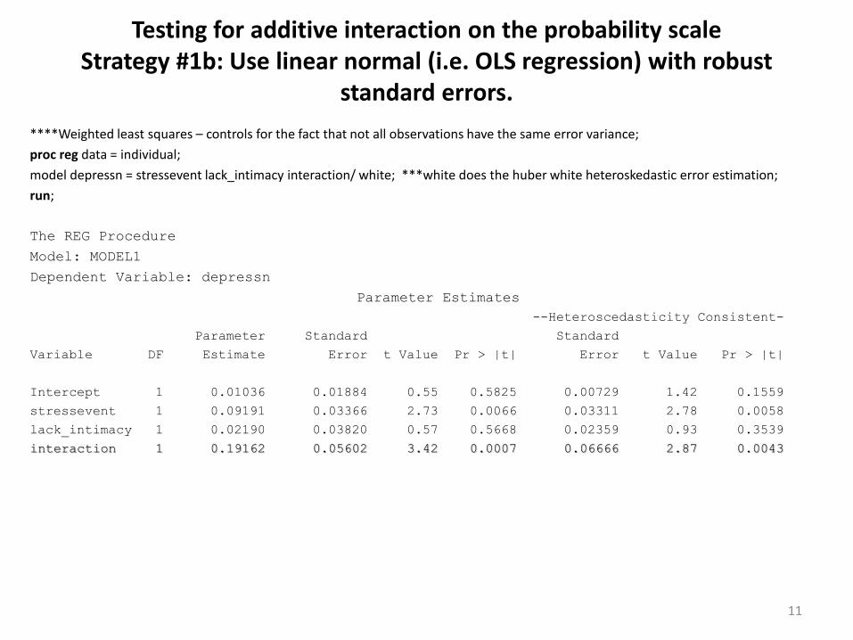
****Weighted least squares – controls for the fact that not all observations have the same error variance;

proc reg data = individual;

model depressn = stressevent lack_intimacy interaction/ white; ***white does the huber white heteroskedastic error estimation;

run;

The REG Procedure

Model: MODEL1

Dependent Variable: depressn

Parameter Estimates

--Heteroscedasticity Consistent-

Parameter Standard Standard

Variable DF Estimate Error t Value Pr > |t| Error t Value Pr > |t|

Intercept 1 0.01036 0.01884 0.55 0.5825 0.00729 1.42 0.1559

stressevent 1 0.09191 0.03366 2.73 0.0066 0.03311 2.78 0.0058

lack_intimacy 1 0.02190 0.03820 0.57 0.5668 0.02359 0.93 0.3539

interaction 1 0.19162 0.05602 3.42 0.0007 0.06666 2.87 0.0043

11

Testing for additive interaction on the probability scale Strategy #1b: Use linear normal (i.e. OLS regression) with robust

standard errors.

Test for additive interaction on the probability scale Strategy #2: Use logistic regression and back-transform estimates

to form contrasts on the probability scale PROC NLMIXED DATA=individual; ***logistic regression model is; odds = exp(b0 +b1*stressevent + b2*lack_intimacy + b3*stressevent*lack_intimacy); pi = odds/(1+odds); MODEL depressn~BINARY(pi); estimate 'p00' exp(b0)/(1+exp(b0)); estimate 'p01' exp(b0+b1)/(1+exp(b0+b1)); estimate 'p10' exp(b0+b2)/(1+exp(b0+b2)); estimate 'p11' exp(b0+b1+b2+b3)/(1+exp(b0+b1+b2+b3)); estimate 'p11-p10' exp(b0+b1+b2+b3)/(1+exp(b0+b1+ b2+b3))- exp(b0+b2)/(1+exp(b0+b2)); estimate 'p01-p00' exp(b0+b1)/(1+exp(b0+b1)) - exp(b0)/(1+exp(b0)); estimate 'IC= interaction contrast = p11-p10 - p01 + p00' exp(b0+b1+b2+b3)/(1+exp(b0+b1+ b2+b3)) - exp(b0+b2)/(1+exp(b0+b2)) - exp(b0+b1)/(1+exp(b0+b1)) + exp(b0)/(1+exp(b0)); estimate 'ICR= RERI using RR = p11/p00 - p10/p00 - p01/p00 + 1' exp(b0+b1+b2+b3)/(1+exp(b0+b1+ b2+b3))/ (exp(b0)/(1+exp(b0))) - exp(b0+b2)/(1+exp(b0+b2))/ (exp(b0)/(1+exp(b0))) - exp(b0+b1)/(1+exp(b0+b1)) / (exp(b0)/(1+exp(b0))) + 1; estimate 'ICR= RERI using OR' exp(b1+b2+b3) - exp(b1) - exp(b2) +1; RUN; 12

These are Strategy #3

Strategy #2 Output from NLMIXED

Parameter Estimates

Standard

Parameter Estimate Error DF t Value Pr > |t| Alpha Lower Upper Gradient

b0 -4.5591 0.7108 419 -6.41 <.0001 0.05 -5.9563 -3.1620 -0.00002

b1 2.3869 0.7931 419 3.01 0.0028 0.05 0.8280 3.9458 -0.00003

b2 1.1579 1.0109 419 1.15 0.2527 0.05 -0.8291 3.1450 2.705E-6

b3 0.2411 1.0984 419 0.22 0.8264 0.05 -1.9180 2.4002 -0.00001

Additional Estimates

Standard

Label Estimate Error DF t Value Pr > |t| Lower Upper

p00 0.01036 0.00728 419 1.42 0.1559 -0.00397 0.0246

p10 0.1023 0.03230 419 3.17 0.0017 0.03878 0.1658

p01 0.03226 0.02244 419 1.44 0.1513 -0.01185 0.0763

p11 0.3158 0.05332 419 5.92 <.0001 0.2110 0.4206

p11-p10 0.2135 0.06234 419 3.43 0.0007 0.09098 0.3361

p01-p00 0.02190 0.02359 419 0.93 0.3539 -0.02448 0.0682

IC =p11-p10-p01+p00 0.1916 0.06666 419 2.87 0.0042 0.06060 0.3226

RERI using RR 18.4915 13.8661 419 1.33 0.1831 -8.7644 45.7473

RERI using OR 31.0138 24.3583 419 1.27 0.2036 -16.8659 78.8936

13

• The IC estimator is same as before (slide 9) but slightly different s.e., p-value and 95% confidence interval – still conclude there is a significant additive interaction.

• Results for RERI (using RR and OR) indicate that there is NOT a significant additive interaction. This conflicts with the conclusion that the IC is highly significant. The cause of the discrepancy is related to estimation of standard errors and confidence intervals. Literature indicates Wald-type confidence intervals perform poorly for RERI (Hosmer and Lemeshow 1992; Assman et al 1996).

• Proc NLMIXED uses Delta method to obtain standard errors of back-transformed parameters and Wald-type confidence intervals, i.e. (estimate) +- 1.96*(standard error) . Possible to obtain profile likelihood confidence intervals using a separate macro (Richardson and Kaufman 2009) or PROC NLP (nonlinear programming) (Kuss et al 2010). Also possible to bootstrap (Assman et al 1996 and Nie et al 2010) or incorporate prior information (Chu et al 2011)

IC estimator same as strategy #1, but slightly different s.e., p-value, 95% conf interval

proc rlogist data = a design = srs; ***srs tells SUDAAN to treat as iid data;

class gene expo ;

reflevel gene=0 expo=0;

model outcome= gene expo gene*expo;

************;

predMARG gene*expo;

pred_eff gene=(1 0)*expo=(-1 1)/name ="pred: exposure effect when gene not present";

pred_eff gene=(0 1)*expo=(-1 1)/name ="pred: exposure effect when gene is present";

pred_eff gene=(-1 1)*expo=(-1 1)/name ="pred_int: difference in risk differences";

**************;

condMARG gene*expo;

cond_eff gene=(1 0)*expo=(-1 1)/name ="cond: exposure effect when gene not present";

cond_eff gene=(0 1)*expo=(-1 1)/name ="cond: exposure effect when gene is present";

cond_eff gene=(-1 1)*expo=(-1 1)/name ="cond_int: difference in risk differences";

run;

14

Test for additive interaction on the probability scale Strategy #2: Use logistic regression and back-transform –

An easier way in SUDAAN

These are the same if there are no covariates

S U D A A N

Software for the Statistical Analysis of Correlated Data

Copyright Research Triangle Institute August 2008

Release 10.0

DESIGN SUMMARY: Variances will be computed using the Taylor Linearization Method, Assuming a

Simple Random Sample (SRS) Design

Number of zero responses : 382

Number of non-zero responses : 37

Response variable OUTCOME: OUTCOME

by: Predicted Marginal #1.

--------------------------------------------------------------------------------

PredMarginal Predicted

#1 Marginal SE T:Marg=0 P-value

--------------------------------------------------------------------------------

GENE, EXPO

0, 0 0.0103626943 0.0072981803 1.4199011081 0.1563818430

0, 1 0.1022727273 0.0323392291 3.1624973812 0.0016782922

1, 0 0.0322580645 0.0224658037 1.4358740502 0.1517860946

1, 1 0.3157894737 0.0533833440 5.9155056648 0.0000000069

--------------------------------------------------------------------------------

--------------------------------------------------------------------------------

Contrasted

Pred Marg#1 PREDMARG

#1 Contrast SE T-Stat P-value

--------------------------------------------------------------------------------

pred:

exposure

effect

when gene

not

present 0.0919100330 0.0331525138 2.7723397823 0.0058143088

--------------------------------------------------------------------------------

15

NOTE: I renamed Gene = lack_intimacy Expo = stress_event But data is same as Brown Harris

More SUDAAN output for the BrownHarris example

--------------------------------------------------------------------------------

Contrasted

Predicted

Marginal PREDMARG

#2 Contrast SE T-Stat P-value

--------------------------------------------------------------------------------

pred:

exposure

effect

when gene

is present 0.2835314092 0.0579179916 4.8953943573 0.0000014039

--------------------------------------------------------------------------------

--------------------------------------------------------------------------------

Contrasted

Predicted

Marginal PREDMARG

#3 Contrast SE T-Stat P-value

--------------------------------------------------------------------------------

pred_int:

difference

in risk

differenc-

es 0.1916213762 0.0667351701 2.8713701643 0.0042948171

-----------------------------------------------------------------------

16

IC

Controlling for Covariates within the back-transformation strategy

• When we fit a model on the logit scale and include a covariate (e.g. age as a main effect) logit p = b0 + b1 * EXPO + b2 * VULN + b3*EXPO*VULN + b4*Gender

this is controlling for gender on the logit scale so that the effects we find for expo, vuln, and expo*vuln on the logit scale (odds ratios) are expected to be the same both genders.

• BUT, back on the probability scale (after back-transformation), the effect of expo, vuln, or expo*vuln will differ depending on which gender someone is

• That is, there was “homogeneity” of effects (across gender) on the logit scale, but there will not be “homogeneity” of effects on the probability scale.

• Not sure this if this is a problem per se but it is something necessary to consider for interpretation.

17

Two ways to back transform – SUDAAN calls them “conditional and predicted” marginal

18

Bieler (2010) Standardized population averaged risk Greenland (2004)

From p.513 SUDAAN manual

Back-transform an “average person”

Two ways of back-transforming…

• The conditional marginal approach estimates the effects on the probability scale for a certain fixed covariate value, usually the mean, but usually an “average person” doesn’t exist, e.g. if the covariate is gender and if 30% of sample is male, this means we are finding the predicted probability associated with someone who is 30% male. Further, if we used some other fixed values for the covariates, we would get different effects (on the probability scale) for the gene*environment

• The predicted marginal approach allows different covariate values to give different predicted probabilities and thus gets a distribution of risks and then averages over them on the probability scale. SUDAAN uses the observed distribution of the covariates in the sample as the “standardization population”, but I believe Sharon Schwartz would argue that perhaps it is better to use the distribution of the covariates in the “unexposed” population to standardize to. I think she had a student work on this for topic and they are working on a paper now.

• From my reading of the EPI literature, the predicted marginal approach is preferred since it has a more meaningful interpretation.

19

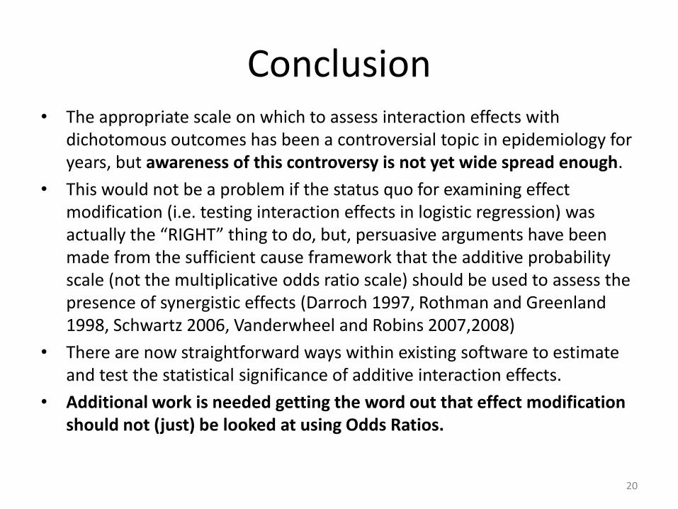
Conclusion • The appropriate scale on which to assess interaction effects with

dichotomous outcomes has been a controversial topic in epidemiology for years, but awareness of this controversy is not yet wide spread enough.

• This would not be a problem if the status quo for examining effect modification (i.e. testing interaction effects in logistic regression) was actually the “RIGHT” thing to do, but, persuasive arguments have been made from the sufficient cause framework that the additive probability scale (not the multiplicative odds ratio scale) should be used to assess the presence of synergistic effects (Darroch 1997, Rothman and Greenland 1998, Schwartz 2006, Vanderwheel and Robins 2007,2008)

• There are now straightforward ways within existing software to estimate and test the statistical significance of additive interaction effects.

• Additional work is needed getting the word out that effect modification should not (just) be looked at using Odds Ratios.

20

1

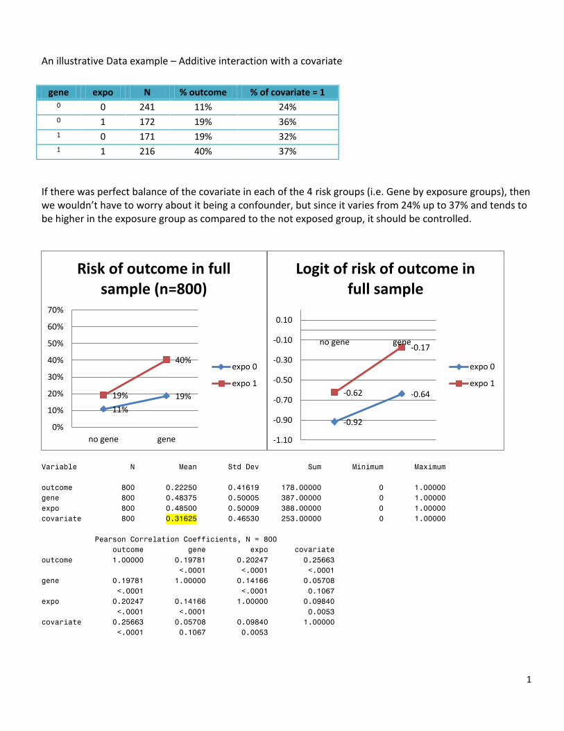
An illustrative Data example – Additive interaction with a covariate

If there was perfect balance of the covariate in each of the 4 risk groups (i.e. Gene by exposure groups), then we wouldn’t have to worry about it being a confounder, but since it varies from 24% up to 37% and tends to be higher in the exposure group as compared to the not exposed group, it should be controlled.

Variable N Mean Std Dev Sum Minimum Maximum

outcome 800 0.22250 0.41619 178.00000 0 1.00000

gene 800 0.48375 0.50005 387.00000 0 1.00000

expo 800 0.48500 0.50009 388.00000 0 1.00000

covariate 800 0.31625 0.46530 253.00000 0 1.00000

Pearson Correlation Coefficients, N = 800

outcome gene expo covariate

outcome 1.00000 0.19781 0.20247 0.25663

<.0001 <.0001 <.0001

gene 0.19781 1.00000 0.14166 0.05708

<.0001 <.0001 0.1067

expo 0.20247 0.14166 1.00000 0.09840

<.0001 <.0001 0.0053

covariate 0.25663 0.05708 0.09840 1.00000

<.0001 0.1067 0.0053

11%

19% 19%

40%

0%

10%

20%

30%

40%

50%

60%

70%

no gene gene

Risk of outcome in full sample (n=800)

expo 0

expo 1

-0.92

-0.64 -0.62

-0.17

-1.10

-0.90

-0.70

-0.50

-0.30

-0.10

0.10

no gene gene

Logit of risk of outcome in full sample

expo 0

expo 1

gene expo N % outcome % of covariate = 1 0 0 241 11% 24% 0 1 172 19% 36% 1 0 171 19% 32% 1 1 216 40% 37%

2

Logistic regression estimates:

Analysis Of Maximum Likelihood Parameter Estimates

Standard Likelihood Ratio 95% Wald

Parameter DF Estimate Error Confidence Limits Chi-Square Pr > ChiSq

Intercept 1 -2.5218 0.2264 -2.9885 -2.0983 124.09 <.0001

gene 1 0.5668 0.2926 -0.0050 1.1462 3.75 0.0527

expo 1 0.5383 0.2913 -0.0309 1.1155 3.41 0.0647

gene*expo 1 0.5514 0.3839 -0.2001 1.3075 2.06 0.1509

covariate 1 1.2192 0.1846 0.8589 1.5835 43.60 <.0001

Scale 0 1.0000 0.0000 1.0000 1.0000

Logit P = -2.52 + 0.5668*GENE + 0.5383*EXPO + 0.5514*G*E + 1.219*Covariate

19%

34% 32%

60%

0%

10%

20%

30%

40%

50%

60%

70%

expo 0 expo 1

Risk when Covariate = 1 (31.6% of sample)

no gene

gene

8% 11%

13%

29%

0%

10%

20%

30%

40%

50%

60%

70%

expo 0 expo 1

Risk when Covariate= 0 (58.4% of sample)

no gene

gene

-0.63

-0.34 -0.29

0.17

-1.10

-0.90

-0.70

-0.50

-0.30

-0.10

0.10

no gene gene

Logit risk Covariate = 1

expo 0

expo 1

-1.05

-0.83 -0.91

-0.38

-1.10

-0.90

-0.70

-0.50

-0.30

-0.10

0.10

no gene gene

Logit risk Covariate = 0

expo 0

expo 1

3

The conditional marginal approach then calculates the predicted

probabilities for the G*E back on the original scale as

> gene=c(0,0,1,1)

> expo=c(0,1,0,1)

> covariate = .31625

> LogitP = -2.52 + 0.5668*gene + 0.5383*expo + 0.5514*gene*expo + 1.219*covariate

> LogitP

[1] -2.1344912 -1.5961912 -1.5676912 -0.4779913

> exp(LogitP)/(1+exp(LogitP))

[1] 0.1057894 0.1685146 0.1725458 0.3827266

FROM SUDAAN

-------------------------------------------------------------------------

Conditional

Marginal Conditional

#1 Marginal SE T:Marg=0 P-value

--------------------------------------------------------------------------------

GENE, EXPO

0, 0 0.1056206853 0.0203578588 5.1882020754 0.0000002694

0, 1 0.1682595536 0.0280578276 5.9968845713 0.0000000030

1, 0 0.1722933591 0.0292915541 5.8820149491 0.0000000060

1, 1 0.3823099821 0.0342856575 11.1507262872 0.0000000000

IC = (.38 - .17) – (.168 - .105)

--------------------------------------------------------------------------------

Contrasted

Condition-

al

Marginal CONDMARG

#3 Contrast SE T-Stat P-value

--------------------------------------------------------------------------------

cond_int:

difference

in risk

differenc-

es 0.1473777547 0.0563674058 2.6145917595 0.0091017247

-----------------------------------------------------------------------------

4

And for the predicted marginal approach we take

> gene=c(0,0,1,1,0,0,1,1)

> expo=c(0,1,0,1,0,1,0,1)

> covariate = c(0,0,0,0,1,1,1,1)

> #covariate = .31625

> LogitP = -2.52 + 0.5668*gene + 0.5383*expo + 0.5514*gene*expo + 1.219*covariate

> LogitP

[1] -2.5200 -1.9817 -1.9532 -0.8635 -1.3010 -0.7627 -0.7342 0.3555

> prob=exp(LogitP)/(1+exp(LogitP))

> prob

[1] 0.07446795 0.12113773 0.12420485 0.29660861 0.21399677 0.31806035 0.32427374

[8] 0.58795068

> predmarg = (1-.31625)*prob[1:4] + .31625*prob[5:8]

> predmarg

[1] 0.1185939 0.1834145 0.1874766 0.3887455

---------------------------------------------------------------------------

Predicted

Marginal Predicted

#1 Marginal SE T:Marg=0 P-value

--------------------------------------------------------------------------------

GENE, EXPO

0, 0 0.1184185808 0.0214723290 5.5149388193 0.0000000471

0, 1 0.1831610712 0.0281468459 6.5073391217 0.0000000001

1, 0 0.1872265641 0.0292713633 6.3962365483 0.0000000003

1, 1 0.3883600906 0.0320980597 12.0991765126 0.0000000000

IC = .388 - .187 – (.183 - .118) = .136

--------------------------------------------------------------------------------

Contrasted

Predicted

Marginal PREDMARG

#3 Contrast SE T-Stat P-value

--------------------------------------------------------------------------------

pred_int:

difference

in risk

differenc-

es 0.1363910361 0.0555247836 2.4563992369 0.0142454402

--------------------------------------------------------------------------------