
Are we going to survive? · Are we going to survive? Economic models of endogenous growth and...
20
Are we going to survive? Economic models of endogenous growth and evidence from global population and CO2 emission trends
Transcript of Are we going to survive? · Are we going to survive? Economic models of endogenous growth and...
Are we going to survive?
Economic models of endogenous growth and evidence from global population and CO2 emission trends
2Andreas HueslerCCSS, 2009-10-24
Outline
Introduction
Economic Model I: IPAT Economic Model II: Cobb-Douglas
Conclusions
Discussion
3Andreas HueslerCCSS, 2009-10-24
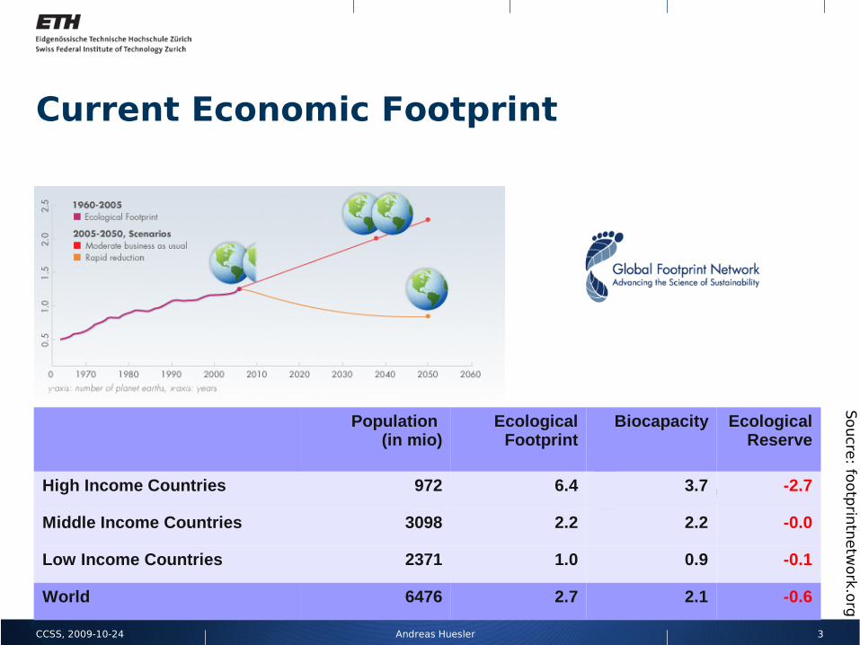
Current Economic Footprint
Population (in mio)
Ecological Footprint
Biocapacity Ecological Reserve
High Income Countries 972 6.4 3.7 -2.7
Middle Income Countries 3098 2.2 2.2 -0.0
Low Income Countries 2371 1.0 0.9 -0.1
World 6476 2.7 2.1 -0.6
Soucre
: footp
rintn
etw
ork
.org

4Andreas HueslerCCSS, 2009-10-24
Planetary Boundaries
Soucre
: doi:1
0.1
038
/461
47
2a

5Andreas HueslerCCSS, 2009-10-24
ImPACT equation I: impact P: population A:affluence C:consumption T: technology
Economic Model I
CO2=Population×GDP
Population×EnergyGDP
×CO2Energy
Soucre
: doi: 1
0.1
07
3

6Andreas HueslerCCSS, 2009-10-24
Growth
Growth description:
Solving ODE:
dpdt
∝ p1
p t =p0tc−t −
0
0
=0
rel.
gro
wth
7Andreas HueslerCCSS, 2009-10-24
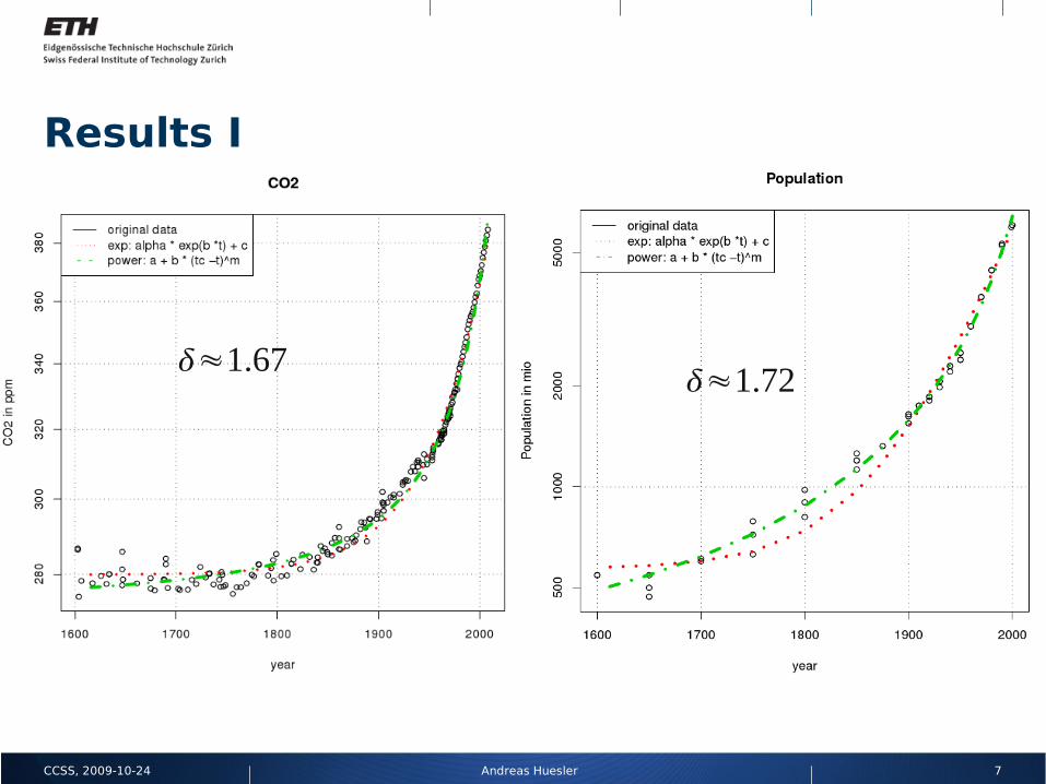
Results I
≈1.67≈1.72

8Andreas HueslerCCSS, 2009-10-24
Results II: Parameter stability
≈1.67
t c=t

9Andreas HueslerCCSS, 2009-10-24
Results II (cont)

10Andreas HueslerCCSS, 2009-10-24
Economic Models II
Cobb-Douglas: Y: output L: labour K: capital A: technology
Solow equation:
Y t =K t ×[ A t Lt ]1−
dAdt
=b K t ×L t ×A t
dKdt
=sY t =s K t ×A t L t 1−
11Andreas HueslerCCSS, 2009-10-24
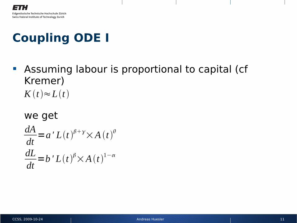
Coupling ODE I
Assuming labour is proportional to capital (cf Kremer)
we getdAdt
=a' L t ×A t
dLdt
=b ' L t ×A t 1−
K t ≈L t
12Andreas HueslerCCSS, 2009-10-24
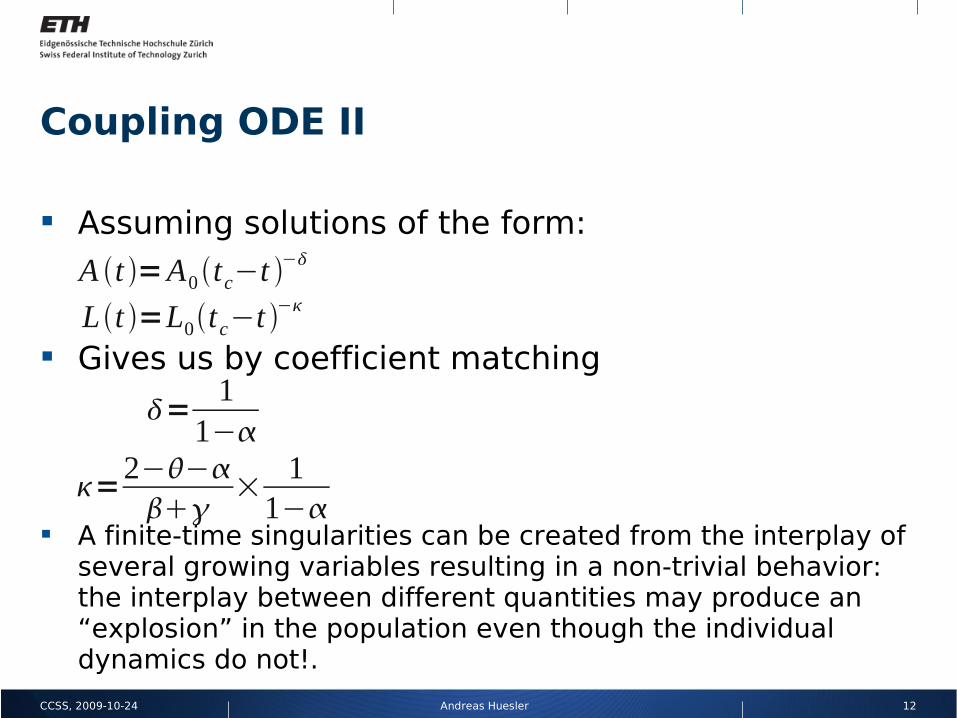
Coupling ODE II
Assuming solutions of the form:
Gives us by coefficient matching
A finite-time singularities can be created from the interplay of several growing variables resulting in a non-trivial behavior: the interplay between different quantities may produce an “explosion” in the population even though the individual dynamics do not!.
A t =A0 tc−t −
L t =L0tc−t −
=11−
=2−−
×
11−
13Andreas HueslerCCSS, 2009-10-24
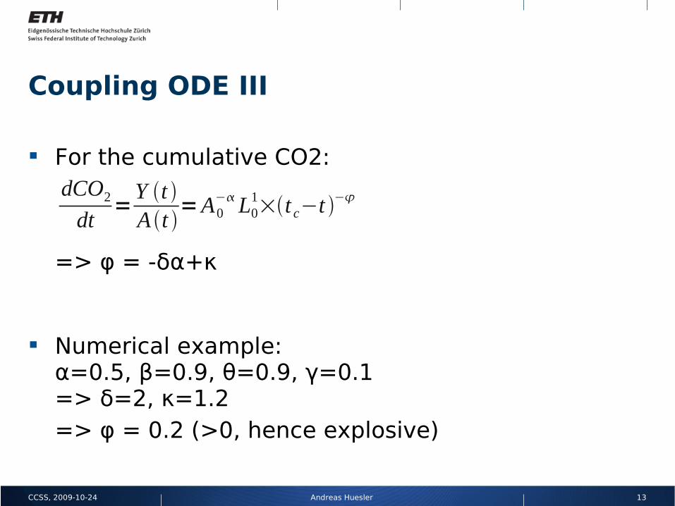
Coupling ODE III
For the cumulative CO2:
=> φ = -δα+κ
Numerical example:α=0.5, β=0.9, θ=0.9, γ=0.1=> δ=2, κ=1.2=> φ = 0.2 (>0, hence explosive)
dCO2dt
=Y t A t
=A0− L0
1×t c−t
−
14Andreas HueslerCCSS, 2009-10-24
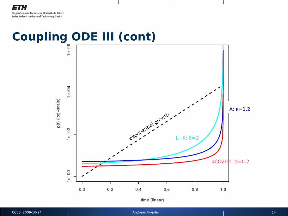
Coupling ODE III (cont)
exponential g
rowth
L~K: δ=2
A: κ=1.2
dCO2/dt: φ=0.2

15Andreas HueslerCCSS, 2009-10-24
Conclusions
Dynamics of CO2 emissions can have complicated dynamics
The (non-linear) dynamics can lead to finite time singularities
Any scenario for future CO2 emissions should take econmic and population dynamics into account.
16Andreas HueslerCCSS, 2009-10-24
References
More references available at:http://www.citeulike.org/user/ahuesler

17Andreas HueslerCCSS, 2009-10-24
Reserve ....
18Andreas HueslerCCSS, 2009-10-24
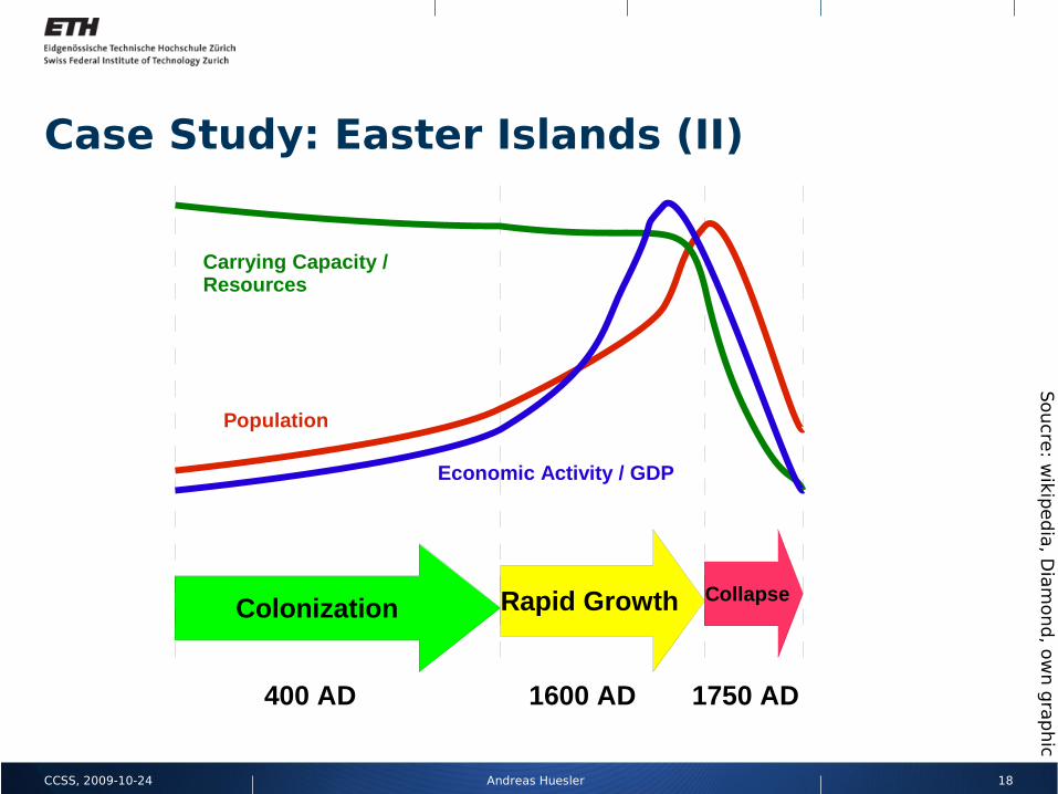
Case Study: Easter Islands (II)
Colonization Rapid Growth Collapse
Carrying Capacity / Resources
Economic Activity / GDP
Population
400 AD 1600 AD 1750 AD
Soucre
: wikip
edia
, Dia
mond, o
wn g
raphic
19Andreas HueslerCCSS, 2009-10-24
20Andreas HueslerCCSS, 2009-10-24
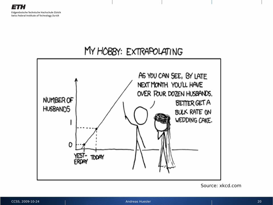
Source: xkcd.com